consume now or later? time inconsistency, collective
TRANSCRIPT

Consume now or later? Time inconsistency, collective choice and revealed preference
IFS Working Paper W14/08
Abi Adams Laurens CherchyeBram De RockEwout Verriest

The Institute for Fiscal Studies (IFS) is an independent research institute whose remit is to carry out
rigorous economic research into public policy and to disseminate the findings of this research. IFS
receives generous support from the Economic and Social Research Council, in particular via the ESRC
Centre for the Microeconomic Analysis of Public Policy (CPP). The content of our working papers is
the work of their authors and does not necessarily represent the views of IFS research staff or
affiliates.

Consume Now or Later?
Time Inconsistency, Collective Choice and Revealed
Preference∗
Abi Adams† Laurens Cherchye‡ Bram De Rock§
Ewout Verriest¶
May 9, 2014
Abstract
In this paper, we develop a revealed preference methodology that allows us to
explore whether time inconsistencies in household choice are the product of in-
dividual preference nonstationarities or the result of individual heterogeneity and
renegotiation within the collective unit. An empirical application to household-level
microdata highlights that an explicit recognition of the collective nature of house-
hold choice enables the vast majority of observed behaviour to be rationalised by a
theory that assumes preference stationarity at the individual level. The methodol-
ogy created in this paper also facilitates the recovery of theory-consistent discount
rates for each individual within a particular household under study. We find that
∗We are grateful to the Editor Larry Samuelson and three anonymous referees for many helpfulcomments, which substantially improved the paper. We also thank Richard Blundell, Ian Crawford,Vincent Crawford, Thomas Demuynck, David Gill, Vijay Krishna, Imran Rasul and seminar participantsin Brussels, New York, Ghent, Royal Holloway and Oxford for useful discussion. Finally, we thank theInstitute for Fiscal Studies for providing access to the household microdata used in this paper. Theauthors declare that they have no relevant or material financial interests that relate to the researchdescribed in this paper.†Department of Economics, University of Oxford, Manor Road Building, Manor Road, Oxford OX1
3UQ, United Kingdom and Institute for Fiscal Studies, 7 Ridgmount Street, London WC1E 7AE. E-mail:[email protected].‡Center for Economic Studies, University of Leuven. E. Sabbelaan 53, B-8500 Kortrijk, Belgium.
E-mail: [email protected]. Laurens Cherchye gratefully acknowledges the EuropeanResearch Council (ERC) for his Consolidator Grant and the Research Fund K.U.Leuven for the grantSTRT1/08/004.§ECARES, Universite Libre de Bruxelles. Avenue F. D. Roosevelt 50, CP 114, B-1050 Brussels,
Belgium. E-mail: [email protected]. Bram De Rock gratefully acknowledges the European ResearchCouncil (ERC) for his Starting Grant and BELSPO for the grant BR/121/A5/MEQIN.¶Center for Economic Studies, University of Leuven. E. Sabbelaan 53, B-8500 Kortrijk, Belgium.
E-mail: [email protected]. Ewout Verriest gratefully acknowledges the Fund for Sci-entific Research - Flanders (FWO-Vlaanderen) for financial support.
1

couples characterised by lower divergence in spousal discount rates are older, which
we take as an indication of experiencing higher match quality.
JEL Classification: D11, D12, D13, C14.
Keywords: time consistency, collective choice, full efficiency, renegotiation, re-
vealed preference.
1 Introduction
In this paper, we consider the extent to which patterns in household intertemporal choice
can be rationalised by simple economic models that assume time consistency at the
individual level. Our analysis reveals that standard models that assume exponential
discounting are consistent with observed household consumption so long as they are
applied to the appropriate decision making unit, i.e. the individual.
Samuelson’s (1937) canonical “discounted utility” (DU) model is the standard frame-
work by which economists conceptualise intertemporal choice. Under this model, a de-
cision maker’s time preferences are captured by a single, time invariant discount rate
and are time consistent. Intuitively, preferences are time consistent if the choice between
alternatives does not depend on when in time that choice occurs: if receiving X at t is
preferred to receiving Y at t + d, the decision maker will always prefer X at τ to Y at
τ + d.
Although the DU model is applied widely because of its tractability, the predictive
validity of the model is thought to be on fragile footing. In experimental settings, decision
makers are often found to behave in a time inconsistent manner, with individuals acting
impatiently in the current moment whilst planning to act patiently in the future. For
example, an individual may prefer to receive $100 today over receiving $110 tomorrow,
whilst simultaneously preferring receiving $110 in 31 days to receiving $100 in 30 days.
Preference reversals such as this are well documented in the psychology and economics
literature (for a survey, see Frederick et al. 2002) but can not be rationalised by a
straightforward application of the DU model.
Research effort has largely focused on modelling the sources of time inconsistent be-
haviour at the individual level. Standard methods of modelling discounting have been a
prime target of criticism, with the behavioural economics literature increasingly favour-
ing frameworks that assume hyperbolic discount functions. Hyperbolic discount functions
are characterised by a relatively high discount rate over short horizons and a relatively
low rate over long horizons. This lack of constancy in the discount rate introduces
a conflict between today’s preferences and future preferences, and a “present bias” to
decision making. Hyperbolic discounting has been offered as an explanation for many
stylised facts, from under-saving and excess co-movement of income and consumption
(Laibson 1997, 1998; Angeletos et al. 2001) to procrastination, addiction and lack of
2

exercise (O’Donoghue and Rabin 1999, 2001; Gruber and Koszegi 2000; DellaVigna and
Malmendier 2006).
In this paper we take a different approach. We consider how acknowledging the collec-
tive nature of choice can rationalise time inconsistencies in non-experimental household
consumption patterns. The preference structure associated with the DU approach is often
applied to model group behaviour without modification. Under this “unitary” approach,
one assumes that the collective acts as a single decision making unit, and therefore can
be treated as if a rational individual. No explicit allowance is made for the separateness
of persons nor preference heterogeneity within a group.
Acknowledgement of the collective nature of choice can rationalise apparent time in-
consistencies in household behaviour. Deriving a time independent discount rate from the
underlying preferences of a heterogeneous population has long been recognised as prob-
lematic (Marglin 1963; Feldstein 1964). When time preferences within a group differ, the
collective preference is typically time inconsistent, even when the underlying population
has perfectly time consistent preferences (Zuber 2011; Jackson and Yariv 2012). In fact,
Jackson and Yariv (2012) show that, with a uniform distribution of discount rates in
an otherwise homogeneous population, group utility maximisation generates aggregate
behaviour that corresponds to hyperbolic discounting.
Furthermore, renegotiations of the household choice rule can also generate nonsta-
tionarities in family behaviour. Relative decision making power within the collective unit
can vary, and differences in time preferences can prompt periodic innovations in the in-
trahousehold preference weighting. Other things equal, it is optimal to relatively favour
impatient group members in early periods and patient members in later periods. However,
as time passes and impatient members begin to receive lower shares of the group surplus,
there is an incentive for them to demand a renegotiation of allocations in their favour
or threaten to leave the group. Renegotiations prompt changes in the intra-household
preference weighting, generating nonstationarities in the collective preference.
Although it is true that nonstationarities at the individual level will translate into
a failure of time consistency at the collective level, understanding whether the primary
locus of inconsistent behaviour is at the self or group level is important from both a
methodological and policy perspective. The DU preference structure is tractable and
parsimonious. Thus, if it cannot be rejected on the basis of choice behaviour, there
are compelling analytic reasons for its retention. Further, policy design should be in-
fluenced according to whether time inconsistent behaviour is the product of individual
nonstationarities or collective aggregation issues.
Methodological contribution. This paper puts forward a nonparametric characteri-
sation of household intertemporal choice and develops a revealed preference methodology
for analysing the sources of time inconsistent collective choice. Our approach follows in
3

the spirit of Afriat (1967), Diewert (1973), and Varian (1982) and incorporates insights
gained from the extension of the revealed preference methodology to an intertemporal
setting by Browning (1989) and Crawford (2010), and to the collective model by Cher-
chye, De Rock and Vermeulen (2007, 2009). The framework presented allows us to
explore whether time inconsistencies in household choice can be rationalised by prefer-
ence heterogeneity and renegotiation within the collective unit rather than individual
nonstationarities. Further, our methodology allows for the recovery of theory-consistent
spousal discount rates and an assessment of the degree of intrahousehold commitment.
This provides the basis for additional analysis on time preference heterogeneity within
the household.
Our methodology is novel in this context and has clear advantages over existing em-
pirical tests of time consistency and household intertemporal behaviour. Current tests
of dynamic collective choice models and time discounting are parametric and tend to
reject the assumptions of constant discounting (see Frederick et al. 2002) and a time-
independent intrahousehold preference weighting (Mazzocco 2007). However, such studies
are sensitive to the parametric specification employed. The common assumption of linear
consumption utility imparts an upward bias to discount rate estimates and is thought to
contribute to the unrealistically high discount rates observed in the literature. Although
recent developments have seen the linear-utility specification somewhat relaxed (Ander-
sen et al. 2012, Andreoni and Sprenger 2012), estimates are still dependent on the set of
functional form assumptions made concerning the form of the utility function. Further,
the experimental nature of existing time discounting studies can be critiqued. Dohman et
al. (2012) highlight that elicited preferences are not procedurally independent and that
discount rate estimates are hugely sensitive to the experimental design employed.
The methodology and empirical application presented in this paper avoids such criti-
cisms. Our revealed preference approach is wholly nonparametric and, thus, our results
are not contingent on any particular specification of family member utility functions.
Rather than directly estimate the preference parameters that best “fit” with some as-
sumed functional specification, we ask whether there exists a non-empty feasible set to
the system of inequalities that are implied by maximising household behaviour within
the framework imposed by economic theory. The existence of a non-empty feasible set to
these inequalities is then a necessary and sufficient condition for household behaviour and
the theory in question to be consistent. Using this approach, we are able to determine
whether time inconsistencies in the revealed household preference can be explained as
a result of discount rate heterogeneity and imperfect commitment within the collective
unit, or whether one must additionally allow for nonstationarities at the individual level.
Our tests are explicitly designed for use with household consumption data, although
they can be profitably applied to an experimental setting. Our empirical application is
one of the few in recent years to be fully grounded in “real world” household consumption
4

behaviour, rather than make use of preference and choice data that has been elicited in
an artificially constructed environment. This allows us to avoid many of the procedural
nuances that plague experimental studies.
Empirical results. We find that accounting for the collective nature of choice allows
us to rationalise time inconsistencies in aggregate household behaviour without positing
nonstationarities in individual preferences. Simply allowing for some limited heterogene-
ity in familial discount rates allows the behaviour of 97.2% of households in our sample
to be rationalised by standard models of household intertemporal behaviour. Our be-
lief in the validity of this result is strengthened by our finding that the time consistent
model performs well when applied to explain the consumption behaviour of single per-
son households, for whom collective explanations do not apply. We find that the minimal
divergence in spousal discount rates is, in general, not well explained by observable house-
hold characteristics, although older couples require a significantly smaller difference in
their time preferences to rationalise their behaviour.
Outline. The paper proceeds as follows. Section 2 defines time consistency of the collec-
tive preference and outlines the associated revealed preference restrictions for establishing
the time consistency of group choice. Section 3 uses these revealed preference conditions
to evaluate the empirical validity of time consistency for a Spanish panel of household
microdata. Our main conclusion here will be that time consistency is heavily rejected
for couples, even when using nonparametric revealed preference restrictions, but that it
performs significantly better for single person households. Section 4 then explores how a
recognition of the collective nature of household choice can rationalise nonstationarities
in the revealed collective preference and derives a nonparametric methodology for testing
hypotheses on the sources of time inconsistent household behaviour. Section 5 continues
our empirical application and provides strong empirical support for this collective ratio-
nalisation of observed time inconsistencies. Here we also correlate intrahousehold time
preference heterogeneity with observable household characteristics. Section 6 concludes.
The Appendix contains the proofs of our main results and some descriptive statistics for
our data.
2 Time consistency and collective choice
The aim of this paper is to provide a framework for exploring the sources of time in-
consistencies in household choice. Specifically, we wish to determine whether explicitly
accounting for the collective nature of choice can allow one to rationalise patterns of
household behaviour without positing nonstationarities at the individual level. This sec-
tion formally defines the concept of time consistency tested in this paper and derives
5

simple revealed preference conditions that can be used to determine the time consistency
of observed household choice.
2.1 The “collective” preference
Collective intertemporal models explicitly recognise the separateness of persons within
a household h, and allow for complete heterogeneity in family member felicity functions
and discount rates. For notational simplicity, we focus on a two-member household,
constituted of members m ∈ {A,B}. The extension of results to an M -member (M > 2)
household is straightforward.
Individual preferences are represented by a time-additive discounted utility function
that is defined over private and public consumption. We assume N private goods and K
public goods. At a given time t, a household h consumes private quantities qh,At ,qh,Bt ∈RN
+ (with associated discounted prices pt ∈ RN++), and public quantities Qh
t ∈ RK+ (with
associated discounted prices Pt ∈ RK++). Public goods are consumed jointly and non-
exclusively within the household. Each household member m in household h is associated
with a concave and strictly increasing felicity function uh,m and discount rate rh,m ∈[0,∞), such that they evaluate the household stream of public and private consumption
Ch,mij = {qh,mt ,Qh
t }t=i,...,j as:
Uh,m(Ch,mij ) =
j∑t=i
βt−1h,mu
h,m(qh,mt ,Qht ),
where βh,m = 1/(1 + rh,m).
Regarding the aggregate household preference, collective models do not assume a pri-
ori that individual preferences can be aggregated into a single time-independent household
felicity function nor do they specify a single intrahousehold bargaining process. Rather,
collective models simply assume that some cooperative decision making process exists
and that this process leads to Pareto efficient outcomes over the affordable budget set.1
With these assumptions, one can define the relative Pareto weight ωht to summarise the
bargaining process within household h in period t. Then, for a household h, the “collec-
tive preference” over some lifecycle consumption profile Ch = {qh,At ,qh,Bt ,Qht }t∈T , where
T = {1, ..., |T |}, is given by:
Uh(Ch) =∑t∈T
{βt−1h,Au
h,A(qh,At ,Qht ) + ωht β
t−1h,Bu
h,B(qh,Bt ,Qht )},
with ωht = f(Zht ), where Zh
t denotes the set of relevant “distribution factors” at time t
1See, for example, Chiappori (1988, 1992) and Browning and Chiappori (1998) for detailed discussionsof the Pareto efficiency assumption in collective household models. Mazzocco (2007) discusses thisframework in an intertemporal context.
6

for household h. The standard theory places no restrictions on what variables count as
relevant distribution factors, beyond requiring that they are independent of individual
preferences (Browning et al. 1994). We note that this lack of structure makes our non-
parametric framework especially attractive as, unlike parametric tests of intertemporal
behaviour, our methodology does not require a formal specification of the factors that
jointly determine ωht .
2.2 Time consistency
Given a household’s time series of consumption choices, the first question of interest is
whether there exists a time consistent household utility function that could have generated
this choice pattern.
What does it mean for the collective preference to be time consistent? Note that the
collective preference over the consumption stream Chij = {qh,At ,qh,Bt ,Qh
t }t=i,...,j is defined
as:
Uh(Chij) =
j∑t=i
{βt−1h,Au
h,A(qh,At ,Qt) + ωht βt−1h,Bu
h,B(qh,Bt ,Qt)}.
Let Chi′j′ represent an “updated” counterpart of Ch
ij (i, j ∈ T , i < j), which denotes the
consumption streams Chij shifted forward into the future by some amount 0 ≤ τ ≤ |T |−j,
and let {Chij,C
hkl} be the combination of two (non-overlapping) consumption streams Ch
ij
and Chkl (i, j, k, l ∈ T , i < j, k < l and j < k or l < i). Then, we can formally define time
consistency of the collective preference as follows.
Definition 1 The collective preference is time consistent if the following two conditions
are satisfied:
1. For any i, j ∈ T with i < j,
Uh(Chij) > Uh(Ch
ij) if and only if Uh(Chi′j′) > Uh(Ch
i′j′).
2. For any i, j, k, l ∈ T with i < j, k < l and, in addition, j < k or l < i,
Uh({Chij,C
hkl}) > Uh({Ch
ij,Chkl}) if and only if Uh({Ch
ij,Ch
kl}) > Uh({Chij,C
h
kl}).
The first condition in Definition 1 imposes stationarity on the collective preference;
the ranking of consumption streams should not depend on when in time those streams
are situated. The second condition requires that the ranking of consumption streams is
independent of periods with identical consumption bundles.
7

Conditions for time consistency. Results originally given in Koopmans (1960), and
applied to a collective setting by Jackson and Yariv (2012), imply that time consistency
of the collective preference requires the ability to re-express the household preference in
the following format:
Uh(Chij) =
j∑t=i
βt−1h uh(qh,At ,qh,Bt ,Qh
t ),
for βh ∈ (0, 1]. Therefore, the existence of a single, constant household discount rate
and a stationary household felicity function is sufficient for a time consistent collective
preference in our setting.
If the following two conditions hold, then the collective preference can be recast in
the above format.2 First, both household members must discount the future at the same
rate, βh,A = βh,B = βh. Second, the intrahousehold decision making mechanism must
give rise to a constant Pareto weight across the lifetime of the household, i.e. ωht = ωh
for all t. Under these conditions, the lifecycle consumption profile of household h, Ch, is
evaluated as:
Uh(Ch) =∑t∈T
{βt−1h,Au
h,A(qh,At ,Qht ) + ωht β
t−1h,Bu
h,B(qh,Bt ,Qht )}
=∑t∈T
βt−1h uh(qh,At ,qh,Bt ,Qh
t ),
where
uh(qh,At ,qh,Bt ,Qht ) = uh,A(qh,At ,Qh
t ) + ωhuh,B(qh,Bt ,Qht ).
If these two conditions hold, then the household can be modelled as a time consistent
representative agent with a latently separable, time-independent felicity function and
constant discount rate.
2.3 Revealed preference conditions
The revealed preference approach to establishing the time consistency of household be-
haviour asks whether one can find necessary and sufficient conditions under which ob-
served choices can be rationalised by a stationary collective preference subject to the
lifecycle budget constraint.
Following the above, we assume |T | observed consumption choices for any given house-
hold h: T = {1, ..., |T |}. For each observation t, we observe the privately consumed
2As a technical remark, we indicate that these conditions are sufficient but, in general, not necessaryfor time consistency. Specifically, the (only) case where necessity does not hold is where βh,A 6= βh,B butωht = (βh,A/βh,B)t−1, which means that the more patient household member has a steadily decreasing
relative bargaining weight that exactly offsets the difference in patience. This alternative model isempirically indistinguishable from ours, i.e. it implies the exact same testable conditions as the timeconsistency model (see Section 2.3). Clearly, however, this is a very particular (and essentially theoretical)construction, from which we will abstract in what follows.
8

quantities, qht , and the publicly consumed quantities, Qht , as well as the corresponding
(discounted) prices, pt and Pt. This defines a set of observations Sh = {qht ,Qht ; pt,Pt}t∈T .
Note that we only assume that aggregate private quantities qht , but not the individual
private quantities qh,At and qh,Bt (with qh,At + qh,Bt = qht ), are observed. This assumption
is motivated by the fact that, in most household surveys (including the one we use in our
own application), information on “who gets what” is limited and the decomposition of
private consumption into that consumed by household members is generally unobserved.
Then, rationalisation of the data set on household h is defined as follows.
Definition 2 The set of observations on household h, Sh = {qht ,Qht ; pt,Pt}t∈T , can be
rationalised by the time consistency model if there exist, for all t ∈ T , private quantities
qh,At , qh,Bt ∈ RN+ (with qh,At + qh,Bt = qht ) and, in addition, a concave, strictly increasing
felicity function uh and discount factor βh ∈ (0, 1] such that∑t∈T
βt−1h uh(qh,At ,qh,Bt ,Qh
t ) ≥∑t∈T
βt−1h uh(ζAt , ζ
Bt , ζ
ht )
for all affordable consumption plans {ζAt , ζBt , ζht }t∈T (with ζAt , ζBt ∈ RN
+ and ζht ∈ RK+ )
that satisfy ∑t∈T
[p′t(qh,At + qh,Bt ) + P′tQ
ht ] ≥
∑t∈T
[p′t(ζAt + ζBt ) + P′tζ
ht ].
In words, the data can be rationalised by a time consistent household preference if
observed choices maximise discounted lifetime household utility out of affordable lifetime
consumption plans for a stationary collective preference.
Theorem 1 then states the revealed preference conditions for a data rationalisation as
defined above. We refer the reader to Appendix A for proofs of all our main results.
Theorem 1 The set of observations on household h, Sh = {qht ,Qht ; pt,Pt}t∈T , can be
rationalised by the time consistency model if and only if there exist, for all t ∈ T , a utility
number uht ∈ R and a positive constant βh ∈ (0, 1] that, for any s,t ∈ T, satisfy
uhs − uht ≤1
βt−1h
[p′t(qhs − qht ) + P′t(Q
hs −Qh
t )].
Theorem 1 is an equivalence result. In words, if there exists a household discount
factor βh and constants {uht }t∈T such that the stated inequalities hold, then there ex-
ists a stationary household felicity function and discount rate that provide a perfect
within-sample rationalisation of the choices observed for household h. The existence of a
non-empty feasible set to these inequalities implies that one cannot reject the hypothesis
of discount factor homogeneity and a time-invariant Pareto weight within the household.
Determining the actual existence of such a non-empty feasible set is easily done empiri-
9

cally. Conditioning on βh, the inequalities defined by Theorem 1 are linear in unknowns
and can be easily verified using standard linear programming techniques.
3 An empirical test of time consistency
In this section we test the time consistency conditions in Theorem 1 for household panel
data taken from the Spanish Continuous Family Expenditure Survey (the Encuesta Con-
tinua de Presupuestos Familiares, ECPF). We strongly reject the hypothesis of a time
consistent collective preference, as defined above.
We examine the robustness of our rejection of the time consistency model as a ratio-
nalisation of household choice by evaluating the sensitivity of our results to two crucial
underlying assumptions. First, we investigate the possibility that actual behaviour is
effectively time consistent but prices or quantities are measured with error. Ignoring
measurement error is a well-known criticism of revealed preference tests and is often used
as an argument to explain their rejection. However, we find that this alternative ex-
planation does not convincingly rationalise the observed rejections of time consistency.
Second, with respect to our conclusions in Sections 4 and 5, it is important to know if
individual preferences are time consistent and thus that rejections are indeed driven by
the collective nature of household choice. We evaluate the time consistency model for
single person households, and find that the model’s empirical performance is significantly
better in this case than for multi person households. These results motivate our focus on
individual heterogeneity within households as a source of time inconsistency.
3.1 The data
Our empirical analysis uses household level expenditure information from the Spanish
Continuous Family Expenditure Survey (the Encuesta Continua de Presupuestos Famil-
iares, ECPF). The ECPF data set is a rotating panel that is conducted every quarter by
the Spanish Statistics Office (INE). Participating households are surveyed in the same
week of each successive quarter, with each adult family member completing an expen-
diture diary in which they record their spending during the survey week. Appendix B
provides summary statistics on the characteristics of the demographic, expenditure and
price data used in our empirical analysis, but we here document the main restrictions
that we impose upon our sample of households.
The data used are drawn from the period 1985-1997. We do not consider data past
1997 because at this time the Continuous Household Budget Survey (CHBS) replaced the
ECPF. The CHBS aimed to provide estimates of the level and change of the aggregate
cost of the household rather than a detailed breakdown of expenditures at the good level.
Participant households are randomly rotated at a rate of 12.5% each quarter, implying
10
that a household may be observed for at most eight consecutive quarters. However, there
are a sizable number of households who do not complete all eight interviews. To achieve
a large sample size, whilst maintaining a long enough panel to provide the right context
for our intertemporal tests, we consider households that report information for at least
four consecutive quarters.
We further restrict our sample according to certain demographic and employment
characteristics of the household. First, we only consider “married” couples (as opposed
to households composed of a collection of adults), with and without children, with both
members under 65 years old. The restriction to married couples is to ensure that we only
consider collections of individuals who may reasonably be expected to act cooperatively
(in line with our theoretical model). Although we consider households with different
numbers of children, we do require that the number of children in the household is sta-
ble over the period of observation to prevent our results being unduly influenced by the
inevitable disruption and change in household dynamics that occurs upon the birth of a
child. We also require that the employment status of husbands and wives is stable over
time. The requirement of stable employment status is to allow the potential nonsepa-
rability of leisure and consumption to be ignored for the time being, as our theoretical
framework does not presently consider the household labour supply decision.
Regarding the household choice bundle, we consider household choice defined over
a commodity bundle of eight nondurable goods for four consecutive quarters.3 Only
households with positive total expenditures on this sample of goods in each time period
are considered. This final restriction leaves us with a sample of 2083 couples to work
with.
Each good is classified as contributing to either “private” or “public” consumption.
Our bundle of six privately consumed goods (N=6) consists of: 1) Food and non-alcoholic
drinks; 2) Clothing and footwear; 3) Transport; 4) Leisure (cinema, theatre, clubs for
sport); 5) Personal services and 6) Restaurants and bars. The bundle of two publicly
consumed goods (K=2) consists of: 1) Household services (heating, water and furniture
repair) and 2) Petrol. Prices are calculated from published prices aggregated at the
household level to correspond to the listed expenditure categories. In our empirical
application, these prices are discounted by the average nominal interest rate on consumer
loans. Appendix B provides summary statistics on the level and variability of the budget
shares and prices of these goods across the sample.
3.2 Revealed preference tests
Revealed preference tests of a given model are defined by hypotheses of the following
form:
3Thus, we implicitly assume separability between durable and nondurable consumption.
11

H0 : Household behaviour can be rationalised by the model.
H1 : Household behaviour cannot be rationalised by the model.
Therefore, such tests yield “yes/no” answers; either household behaviour is consistent
with the model in question or it is not. A “yes” result implies that the model cannot be
rejected on the basis of observed behaviour. However, it does not necessarily imply that
the model is “the truth”. Popper (1959) points to the logical asymmetry between verifi-
cation and falsification. No number of observed passes of model X allows one to derive
the universal statement: “All households can be rationalised by model X”. However,
failure of a revealed preference test allows us to logically derive the conclusion: “The
household cannot be rationalised by model X”.
As explained in Section 2, testing whether household h’s consumption choices can be
rationalised by a time consistent household utility function boils down to checking the
linear conditions defined by Theorem 1 for a given value of the discount factor βh. In our
empirical application we conduct a grid search on βh for every household h = 1, ..., H.
We report results for a grid search of individual discount factors on [0.9, 1] with a spacing
of 0.005.4 At this point, it is worth noting that all our following results are robust to
alternative grid search specifications (including a grid search across the full interval (0, 1]).
These robustness checks can be obtained from the authors on request.
We also remark here that our tests allow for unrestricted preference heterogeneity
across households, as captured by the individual-specific felicity functions. The theory-
consistency of each household’s behaviour is tested independently and the data is not
pooled at any stage.
Accounting for how “demanding” a test is. An obvious measure for the empirical
performance of a behavioural model is its pass rate, i.e. the number of households in our
sample that pass its testable implications. However, a model’s pass rate only captures
one dimension of its empirical performance. Alongside the pass rate, empirical appli-
cations of revealed preference tests typically report two additional performance metrics:
discriminatory power and predictive success. Predictive success gives a holistic measure
of the empirical performance of a behavioural model by simultaneously accounting for a
model’s pass rate and how “demanding” our test is. As such, we will primarily evaluate
our various behavioural models according to the predictive success metric.
Discriminatory power. Following Bronars (1987), the discriminatory power of a re-
vealed preference test for a particular behavioural model is defined as the probability
of detecting behaviour that is not rationalisable by the model. It, therefore, provides a
measure of how demanding a test is. Bronars suggests an iterative procedure to compute
4This corresponds to a search for discount rate on [0, 0.11], which given the quarterly periodicity ofour data is not unreasonable.
12

his power metric, which we apply to each household in our sample. At every iteration,
the procedure simulates random behaviour (i.e. behaviour that is not generated by any
optimising model) by drawing |T | × (N + K) random budget shares from the uniform
distribution. For a given household h, these budget shares then define a new random
consumption stream {qh,Rt ,Qh,Rt }t∈T that exhausts their total wealth.5 We then test
the revealed preference conditions of the model under evaluation on the correspondingly
defined set {qh,Rt ,Qh,Rt ; pt,Pt}t∈T . In our application, we iterate this procedure 1000
times per household and calculate the proportion of the randomly generated consump-
tion streams that fail the revealed preference restrictions of the behavioural model.
We use the proportion of randomly generated consumption streams that fail the re-
vealed preference restrictions to calculate a household-specific measure for discriminatory
power. This proportion proxies the true probability that random household behaviour
will fail the restrictions of the behavioural model for observed prices and total household
expenditure. For example, if 60% of all randomly generated consumption streams fail
to meet the requirements of a revealed preference test, then there is approximately a
60% chance that our tests will correctly reject random choice behaviour. Generally, high
power signals a restrictive model and there is a high probability that revealed preference
tests will detect irrational/random behaviour.
At this point, recall that we conduct a grid search on the discount factor (βh) to
compute the pass rate for the time consistent model. Computing power requires an anal-
ogous grid search at each iteration. We define a household specific grid size, conditional
on whether a household’s choices are rationalisable by the model under study. If ob-
served behaviour is not rationalisable, then at each iteration we define the same grid size
as before: the interval [0.9, 1] with a spacing of 0.005. However, if household h’s observed
behaviour can be rationalised by the model, we use this information to define a finer grid
when computing their power metric. Specifically, we search only over βh no lower than
the maximum value under which rationalisability is obtained. This adjusted grid search
substantially limits the computational burden of our power assessment, whilst accounting
for the information on individual time preferences as revealed by the observed behaviour.
Predictive success. We primarily evaluate the empirical performance of a model ac-
cording to the value of its predictive success metric. This measure combines the pass
rate and the power of a particular behavioural model into a single metric that can be
interpreted as the power-adjusted pass rate. It was recently axiomatised by Beatty and
Crawford (2011) and is based upon an original proposal of Selten (1991). For each house-
hold, predictive success is calculated by subtracting 1 minus the power measure from the
pass measure (1 or 0). Therefore, the measure is always situated between -1 and 1.
5This simulated random behaviour corresponds to Becker’s (1962) notion of irrational behaviour asbehaviour that randomly exhausts the available budget.
13

The higher the average predictive success measure, the better the empirical perfor-
mance of the behavioural model under evaluation. A predictive success value in the
neighbourhood of -1 indicates that a household fails the rationalisability conditions, im-
plying a pass measure equal to 0, even though the power of the test is low and relatively
easy to pass (i.e. discriminatory power is close to 0). Conversely, a predictive success
value in the neighbourhood of 1 indicates a household that passes the model restrictions
in a situation where the model has high power. This represents the ideal scenario if you
will. Finally, a predictive success value equal to zero suggests that the model is not in-
formative for the household at hand: the model does not outperform the uninformative
assumption that households exhibit random consumption behaviour, for which the power
is 0 and the pass measure equals 1, by construction.
3.3 Test results
Table 1 reports the test results obtained from applying the revealed preference conditions
in Theorem 1 to the ECPF data. We find that only 14% of the 2083 households in our
sample can be rationalised by a time consistent collective preference. This result suggests
that the empirical support for the time consistency model as an explanation for household
choice is weak. However, the revealed preference test of the model is relatively stringent.
On average, the test has an 84% probability of rejecting randomly simulated choice
behaviour. This is very high in comparison to the power metrics typically calculated
for the static collective model, which typically lie in the neighbourhood of zero (see, for
example, Cherchye, De Rock and Vermeulen, 2009).
Table 1: Time consistency model
pass rate power predictive successmean
(st. error)
0.1402(0.0076)
0.8490(0.0008)
-0.0108(0.0082)
Yet, even taking account fo the high demandingness of the test, the empirical perfor-
mance of the time consistency model is poor. The predictive success measure of -0.01
highlights that, on average, households are performing on a par with a random number
generator.
Figure 1 gives the distribution of predictive success that is associated with the time
consistent model. The distribution is bimodal and the fit of the model is very poor for
the majority of households; predictive success is negative for 86% of the households in
our sample. Our predictive success findings suggest that we can safely conclude that the
data does not endorse the applicability of the time consistent model (as it stands) to
14

explain household intertemporal choice behaviour.
3.4 Robustness checks
In this section, we investigate the robustness of the rejection of the time consistency
model as an explanation for household choice behaviour by investigating the impact
of two crucial underlying assumptions. First, we relax the assumption that observed
prices and consumption quantities are unaffected by measurement error. We find that an
allowance for measurement error does not significantly improve the empirical performance
of the model. Second, we examine the empirical validity of the time consistency model
for single person households. This is particularly relevant in view of our discussion in
the following sections, which aims at rationalising time-inconsistency of multi person
households under the maintained assumption that individual household members are
time consistent. Interestingly, we will find that the time consistency model indeed does
perform significantly better for single person households than for multi person households.
Measurement error. The decisive rejection of the time consistency model could be the
result of errors in listed expenditure data, rather than deviations of actual choice from the
model’s prescriptions. Revealed preference tests are “sharp” in that household behaviour
is either consistent with the model in question or it is not. Thus, small deviations in
observed quantities or prices away from the their true values could have a large impact
on predictive success. Moreover, seasonality in our quarterly data might also explain why
time consistency at the household level fails, due to the possible changes in the structure
of consumption across seasons.6 If this is the case for our sample, then introducing a
sufficient amount of measurement error should pick up this effect.
To explore the impact of allowing for measurement error on our test results, we use a
procedure that is based on an original idea of Varian (1985). Essentially, the procedure
evaluates the predictive success of the time consistency model by considering a weaker
test that accounts for possible errors in the data. We consider two exercises. Our first
6At this point, we also note that our use of broad good categories may be expected to considerablymitigate seasonality effects, by construction.
15

exercise considers errors in the quantity data, and our second exercise focuses on errors in
the price data. We cannot consider the impact of allowing for price and quantity errors
simulatenously because this introduces a non-linearity to the procedure, which introduces
a significant computational difficulty.
For compactness, we here explain only our procedure for quantity errors. How-
ever, the reasoning for price errors is directly analogous. Consider a data set Sh =
{qht ,Qht ; pt,Pt}t∈T for a household h that does not meet the conditions defined by Theo-
rem 1. For a household observation t, let qht,n represent the observed quantity of the n-th
private good and Qht,k the observed quantity of the k-th public good. Due to measure-
ment error, these quantities may deviate from qh,∗t,n and Qh,∗t,n , the true (but unobserved)
values of the private and public quantities that are consumed within the household. The
divergence between listed and true quantities are quantified by the “relative quantity
errors”:
εht,n =qh,∗t,n − qht,n
qht,nand εt,k =
Qh,∗t,k −Qh
t,k
Qht,k
As we cannot observe the true values, qh,∗t,n and Qh,∗t,n (or, equivalently, the actual
errors εht,n and εht,k), we approximate the necessary measurement error required for listed
expenditure data to pass the revealed preference conditions. We do this by calculating the
minimal adjustments of the quantity data that are required to obtain theory consistency.
Specifically, we define the following perturbation to observed quantities for each particular
household h:
qht,n =(1 + εht,n
)qht,n and Qh
t,k =(1 + εht,k
)Qht,n,
and minimise the sum of squared error terms for the household :
min Vh=
|T |∑t=1
(N∑n=1
(εht,n)2 +K∑k=1
(εht,k)2
),
subject to the constraint that the perturbed data set Sh = {qht , Qht ; pt,Pt}t∈T satisfies
the model. This effectively calculates the smallest perturbations εht,n and εht,k that are
16

necessary for Sh to be rationalised by the time consistent model.
Using the estimated minimal perturbations, we can compute
σh=
√Vh
|T | ∗ (N +K),
which gives an estimate for the average quantity error that we need to make our data
satisfy the time consistency model. By construction, we will have that σh = 0 if the
original data set Sh meets the conditions in Theorem 1, while higher values of σh indicates
that more measurement error is required to rationalise the observed behaviour as being
time consistent.
If one allows for sufficient measurement error, any behaviour can be classed as con-
sistent with the model. Therefore, we assess the average minimum measurement errors
that are required to rationalise the data relative to particular benchmark upper bounds
on the standard deviation of the measurement error process, σ. Clearly, lower values for
σ obtain more stringent tests, with σ = 0 yielding the original conditions in Theorem 1.
As previously, we account for the trade-off between pass rate and power by evaluating
the predictive success of the time consistency model for alternative σ values.
In Table 2, we report predictive success outcomes for “low” and “high” measurement
error scenarios. We define the upper bound in our low measurement error scenario as the
cut-off value σLO that corresponds to a pass rate of one-third (i.e. σLO is the 33%-quantile
of the empirical distribution of σh).7 In particular, we get the cut-off value σquantLO = 0.05
for quantities and σpriceLO = 0.005 for prices. Our second scenario accounts for a large
amount of measurement error, using a cut-off value σHI that is sufficient to rationalise
the full sample. In this case, we obtain σquantHI = 0.15 for quantities and σpriceHI = 0.1
for prices. The values of these cut-offs, and of the associated predictive success, differ
between measurement error in prices and measurement error in quantities because of
differences in the extent, and nature, of variation of prices and quantities.
7We define this cut-off because it effectively doubles the pass rate of the time consistency model,thereby providing sufficient margin for the predictive success of the model with low measurement errorto dominate that of the time consistency model.
17

Table 2: Measurement error
predictive success
mean st. error.
no measurement error (time consistency) -0.0108 0.0076
measurement error in prices: - low (cut-off σpriceLO ) 0.0426 0.0127
- high (cut-off σpriceHI ) 0.0482 0.0038
measurement error in quantities: - low (cut-off σquantLO ) -0.0898 0.0192
- high (cut-off σquantHI ) 0.0060 0.0214
Neither the predictive success values for measurement error in prices nor quantities
provide strong support for the hypothesis that these errors are primarily responsible for
the poor empirical performance of the time consistency model. All of the predictive
success values in Table 2 remain in the neighbourhood of zero. In our opinion, one may
safely argue that measurement error does not lie behind the poor empirical performance
of the time consistency model.
Single person households. Our data set contains information on a small sample of
single person households. As with our sample of couples, we impose the requirements
of stable employment status, positive expenditures on the considered goods categories,
and that they are aged under 65 for the full length of observations. This leaves us with
a sample of 189 individuals. Our robustness check verifies the conditions in Theorem 1
for each of these 189 individuals to assess whether it is reasonable to assume that singles
indeed behave time consistently.
Interestingly, Table 3 shows that the time consistency hypothesis fits significantly
better for singles than for couples. In particular, for singles we obtain a predictive success
rate that is substantially above zero. This indicates that the model effectively provides
a more informative explanation of the singles’ behaviour in our sample. Furthermore,
this value for predictive success is impressive compared to those associated with other
revealed preference tests. For example, Beatty and Crawford (2010) calculate an average
predictive success measure of 0.045 for the static utility maximisation model on a sample
18

also drawn from the ECPF. Adams (2011) calculates a predictive success measure of
0.000 for the static collective model.
Table 3: Single person households
predictive successmean st. error.
Time consistency - couples -0.0108 0.0076- singles 0.1444 0.0355
We conclude that individual nonstationarities alone cannot fully account for the poor
empirical performance of households when evaluated in line with the time consistency
model. There must be some other force at work. This directly motivates our following
analysis, in which we investigate our core hypothesis that the observed time inconsistency
of couples’ behaviour is in large part due to the multi person nature of household decisions.
4 Collective choice and time inconsistency
The collective preference cannot be recast in the format required for time consistency in
the presence of either heterogeneity in individual time preferences or periodic innovations
in the Pareto weight. The failures of these assumptions manifest themselves in observed
choice behaviour differently. This section explores these sources of time inconsistency
in greater depth and utilises Mazzocco’s (2007) theoretical framework to develop an
empirical strategy for distinguishing between the different sources of time inconsistent
household behaviour.
4.1 Individual heterogeneity
Within household h, individual heterogeneity and innovations in the Pareto weight, ωht ,
can introduce time inconsistencies to household consumption patterns, even if individuals
within the household have perfectly time consistent preferences.
With intrahousehold discount rate heterogeneity, one cannot collapse individual dis-
count rates into a single household rate of time preference, βtA + βtB 6= (βA + βB)t. This
implies that members’ preferences are weighted differently in the household allocation
problem at different points in time, even if the Pareto weight remains constant. Other
19
things equal, the preferences of the more patient member become relatively more impor-
tant in future time periods, introducing a time inconsistency to the collective preference.
Jackson and Yariv (2012) prove that for a group of otherwise homogeneous individuals
choosing a common consumption stream, any heterogeneity in time preferences neces-
sitates a present biased collective preference, and that with a uniform distribution of
discount rates in a population, the collective utility function is hyperbolic. Thus, time
inconsistencies in group behaviour need not be derivative of nonstationarities at the
individual level. Rather, they can arise from the aggregation of heterogeneous time pref-
erences.
The full efficiency model. Individual heterogeneity is the only source of time incon-
sistency in Mazzocco’s (2007) “full efficiency” model. The model assumes the existence
of a perfect commitment mechanism, removing the possibility of intrahousehold rene-
gotiation. This implies the existence of a single, fixed Pareto weight to summarise the
household decision making process.
For a given data set on household h, Sh = {qht ,Qht ; pt,Pt}t∈T , the full efficiency model
corresponds to the following rationalisation condition.8
Definition 3 The set of observations on household h, Sh = {qht ,Qht ; pt,Pt}t∈T , can be
rationalised by the full efficiency model if there exist, for all t ∈ T , private quantities
qh,At , qh,Bt ∈ RN+ (with qh,At + qh,Bt = qht ) and, in addition, concave, strictly increasing
felicity functions uh,A and uh,B, discount factors βh,A, βh,B ∈ (0, 1] and a Pareto weight
ωh > 0 such that
∑t∈T
{βt−1h,Au
h,A(qh,At ,Qht ) + ωhβt−1
h,Buh,B(qh,Bt ,Qh
t )}≥∑t∈T
{βt−1h,Au
h,A(ζAt , ζht ) + ωhβt−1
h,Buh,B(ζBt , ζ
ht )}
for all affordable consumption plans {ζAt , ζBt , ζht }t∈T (with ζAt , ζBt ∈ RN
+ and ζht ∈ RK+ ),
8One important difference between our theoretical framework and that of Mazzocco’s (2007) “fullefficiency” model is the assumption of perfect foresight. Revealed preference tests of martingale processeslack content as, without a specification of the expectation process, one can always posit an unexpectedshock to rationalise behaviour. Following Mazzocco, our framework also assumes perfect capital markets.We recognise that these assumptions are very strong. Still, in our empirical application we will find thatnearly all observed household behaviour in our sample can be rationalised even when maintaining theseassumptions. See Section 5 for a further discussion.
20

which satisfy
∑t∈T
[p′t(qh,At + qh,Bt ) + P′tQ
ht ] ≥
∑t∈T
[p′t(ζAt + ζBt ) + P′tζ
ht ].
As for the time consistent model, the constant Pareto weight ωh incorporates the
combined impact of all changes in distribution factors over time; it can be considered as
the average relative power of family members across the lifetime of the household. In
this setting, the only source of time inconsistent aggregate behaviour is discount rate
heterogeneity. Recall that if βh,A = βh,B = βh, then the collective preference could be
recast in a time consistent format with a stationary household felicity function.
Revealed preference conditions. How can we test for the importance of individual
heterogeneity as a source of time inconsistency? Discount rate heterogeneity negates the
possibility of representing the collective preference in representative-consumer format.
Given this, the composition of household consumption and its distribution between family
members plays a central role in revealed preference tests of the full efficiency model. This
has two important implications for the revealed preference conditions associated with
the full efficiency model. First, for privately consumed goods, the information on qh,At
and qh,Bt is relevant. Second, for publicly consumed goods, the relevant “prices” for an
individual family member will be so-called Lindahl prices, Ph,At and Ph,B
t . These prices
coincide with a family member’s marginal willingness to pay and, given the maintained
assumption of cooperative decision making, sum to observed prices, Ph,At + Ph,B
t = Pt.
Theorem 2 gives the conditions under which household choice can be rationalised by
the full efficiency model. If choices can be rationalised by the model, we cannot reject
the hypothesis that time inconsistencies in aggregate behaviour are the result of discount
rate heterogeneity within the family.
Theorem 2 The set of observations on household h, Sh = {qht ,Qht ; pt,Pt}t∈T can be
rationalised by the full efficiency model if and only if there exist, for all t ∈ T , private
quantities qh,At , qh,Bt ∈ RN+ (with qh,At + qh,Bt = qht ), Lindahl prices Ph,A
t , Ph,Bt ∈ RN
+ (with
21
Ph,At + Ph,B
t = Pht ), utility numbers uh,At , uh,Bt ∈ R and constants βh,A, βh,B ∈ (0, 1] that,
for any s, t ∈ T , satisfy
uh,As − uh,At ≤ 1
βt−1h,A
[p′t(q
h,As − qh,At ) + Ph,A′
t (Qhs −Qh
t )],
uh,Bs − uh,Bt ≤ 1
βt−1h,B
[p′t(q
h,Bs − qh,Bt ) + Ph,B′
t (Qhs −Qh
t )].
In words, if we can find a discount factor βh,m and constants {uh,mt }t∈T for each member
m ∈ {A,B} in household h, along with feasible private quantities and Lindahl prices,
such that the inequalities defined by Theorem 2 hold, then there exists a pair of felicity
functions and constant discount rates that provide a perfect within-sample rationalisation
of the household data. Conversely, if we cannot find values of all relevant variables such
that these inequalities hold, then there does not exist a theory-consistent specification of
household member preferences and a constant Pareto weight that rationalise the observed
consumption stream. This allows us to test whether time inconsistencies in choice can
be explained by appeal to discount rate heterogeneity alone. If a non-empty feasible set
is associated with the full efficiency constraints, one cannot reject the hypothesis that
time inconsistency in household choice is simply the product of individual heterogeneity
within the collective unit; one does not necessarily require nonstationarities in individual
preferences or renegotiations of the household choice rule over time to rationalise the
observed behaviour.
4.2 Renegotiation
If household behaviour is inconsistent with the full efficiency model, an appeal to more
than just discount rate heterogeneity is required. The second condition for time con-
sistency of the collective preference is the existence of a constant Pareto weight across
the full lifetime of the household. Whether this is necessarily attained depends upon
the existence of a perfect intrahousehold commitment mechanism. Without a perfect
commitment device, the Pareto weight can vary over time to reflect renegotiations of the
household choice rule. These renegotiations open up an additional mechanism for time
22

inconsistent behaviour.
The no-commitment model. Mazzocco’s (2007) “no-commitment” model weakens
the assumption of perfect intrahousehold commitment. Instead, the household solves
the lifetime bargaining problem subject to additional incentive compatibility constraints.
Mazzocco (2007) classes a consumption stream as incentive compatible if it does not
provide an incentive for any family member to quit the household at some point to take
their “outside option”. An individual’s outside option is defined as the utility they could
derive from divorcing and continuing in the world alone.9
Using the method developed by Marcet and Marimon (1998), the no-commitment
model can be formulated as a recursive saddle point problem and theory consistent be-
haviour corresponds to the following rationalisation condition.10
Definition 4 The set of observations on household h, Sh = {qht ,Qht ; pt,Pt}t∈T can be
rationalised by the no-commitment model if there exist, for all t ∈ T , private quantities
qh,At , qh,Bt ∈ RN+ (with qh,At + qh,Bt = qht ) and, in addition, concave, strictly increas-
ing felicity functions uh,A and uh,B, discount factors βh,A, βh,B ∈ (0, 1], Pareto weights
ωh,At , ωh,Bt > 0, multipliers ϕh,At and ϕh,Bt and outside utilities uh,At and uh,Bt such that:
∑t∈T
{[ωh,At βt−1
h,Auh,A(qh,At ,Qh
t )− ϕh,At uh,At
]+[ωh,Bt βt−1
h,Buh,B(qh,Bt ,Qh
t )− ϕh,Bt uh,Bt
]}≥
∑t∈T
{[ωh,At βt−1
h,Auh,A(ζAt , ζ
ht )− ϕ
h,At uh,At
]+[ωh,Bt βt−1
h,Buh,B(ζAt , ζ
ht )− ϕ
h,Bt uh,Bt
]}
for all affordable consumption plans {ζAt , ζBt , ζht }t∈T (with ζAt , ζBt ∈ RN
+ and ζht ∈ RK+ ),
9This definition is akin to Shaked and Sutton’s (1984) formulation of outside options.10This formulation implicitly embodies the requirement that a particular consumption profile must be
incentive compatible, i.e. for each member m = {A,B} and t ∈ {1, ..., |T |}
|T |−t∑s=0
βsh,mu
h,m(qh,mt+s ,Q
ht+s) ≥ u
h,mt .
In words, by remaining within the household each household member must achieve welfare at least asgreat as when exiting via divorce.
23

which satisfy
∑t∈T
[p′t(qh,At + qh,Bt ) + P′tQ
ht ] ≥
∑t∈T
[p′t(ζAt + ζBt ) + P′tζ
ht ].
In this definition, ϕh,mt represents the Lagrange multiplier on m’s incentive compati-
bility constraint, and uh,mt gives the utility associated with m’s outside option, that is, the
stream of utility that m could receive when leaving household h at period t. The house-
hold choice rule, summarised by the set of intrahousehold preference weights, ωh,mt , is
sequentially renegotiated to reflect changes in the slackness of the incentive compatibility
constraints: ωh,A1 = 1, ωh,At = ωh,At−1 + ϕh,At and ωh,B1 = ωh, ωh,Bt = ωh,Bt−1 + ϕh,Bt . Assuming
positive gains to marriage continuation for at least one spouse in every time period, there
will always be at least one individual who is strictly better off if the marriage continues
rather than dissolving through divorce. Thus, the incentive compatibility condition can
only bind for one family member at any point in time, i.e. if ϕh,At 6= 0 then ϕh,Bt = 0,
and vice versa. In periods where the incentive compatibility constraint binds for some
member, the weight assigned to her preferences is increased until she is indifferent be-
tween taking their outside option and staying within the household. This new weighting
of family member preferences then prevails in subsequent time periods until an incentive
constraint again binds and another reweighting of preferences is implemented.
Stationarity of the household per-period felicity function can now also be undermined
by renegotiations of the household choice rule, which take place whenever an incentive
compatibility constraint binds. That allocations are sensitive to outside option hetero-
geneity is clear from the family maximisation problem; uh,mt appears explicitly in the
household objective function. However, the interaction between discount rate hetero-
geneity and incentive compatibility is more subtle. Consider a couple who are identical
in every respect except for their patience, βh,A < βh,B. The optimal lifecycle plan would
see a more present-weighted consumption profile for A than B. Thus in early periods,
A would receive a greater relative share of per-period expenditure, and the opposite in
later periods. However, without a commitment mechanism, this plan may be infeasible.
24

In some period, as her per-period resource share drops, A could conceivably do better
by quitting the household, especially given the low weight she attaches to future marital
surpluses. The Pareto weight will then be renegotiated to reemphasise A’s preferences in
the household allocation problem to prevent her from dissolving the household.
Revealed preference conditions. The no-commitment model implies the existence
of a set of mutually exclusive subsets within there is no renegotiation and thus, the same
Pareto weight is applied.11 To introduce the potential for renegotiation into our revealed
preference set-up, consider a partition of the set T into Υ mutually exclusive subsets Tτ
of the form
T = {T1, ..., TΥ},
with
T = ∪Υτ=1Tτ and Tτs ∩ Tτt = ∅ if τs 6= τt,
such that
τ1 < τ2 implies t1 < t2 for all t1 ∈ Tτ1 and t2 ∈ Tτ2 .
Each subset represents a distinct “Pareto weight regime”, thus ωms = ωmt for all s, t ∈ Tτ .
Let the Pareto weight in subset Tτ thus be denoted ωmτ . We then have the following
testability result.
Theorem 3 Given a partition T, the set of observations on household h, Sh = {qht ,Qht ; pt,Pt}t∈T ,
can be rationalised by the no-commitment model only if there exist, for all t ∈ T , private
quantities qh,At , qh,Bt ∈ RN+ (with qh,At + qh,Bt = qht ), Lindahl prices Ph,A
t , Ph,Bt ∈ RN
+ (with
Ph,At + Ph,B
t = Pt), utility numbers uh,At , uh,Bt ∈ R and constants βh,A, βh,B ∈ (0, 1] that,
for any s, t ∈ Tτ (τ ∈ {1, ...,Υ}), satisfy
uh,As − uh,At ≤ 1
βt−1h,A
[p′t(q
h,As − qh,At ) + Ph,A′
t (Qhs −Qh
t )],
uh,Bs − uh,Bt ≤ 1
βt−1h,B
[p′t(q
h,Bs − qh,Bt ) + Ph,B′
t (Qhs −Qh
t )].
11For rich enough data sets we can define these subsets by using information on outside options. Inour own application (in Section 5), however, we do not have such information and, therefore, we considerall possible partitions Th.
25
The interpretation is similar to before. In this particular case, innovations in the
household’s Pareto weight define the partitions of the set T. Thus, within sub-periods Tτ ,
household h’s Pareto weight is constant and choices must satisfy the revealed preference
inequalities associated with the full efficiency model (in Theorem 2).
5 Rationalising observed time inconsistency
In this section, we resume our empirical application using the ECPF data. We find that
simply allowing for limited intrahousehold heterogeneity in the discount rate allows the
behaviour of 97.2% of families to be rationalised without recourse to individual deviations
from exponential discounting. Moreover, and more importantly, the predictive success
of the model amounts to no less than 56.1%. Given this positive result, we conduct a
detailed investigation of the theory-consistent differences in spousal discount rates.
Although the vast majority of household behaviour can be explained without any
mention of intrahousehold renegotiation, we provide results for a strengthened version
of the conditions in Theorem 3, which assumes equal discount factors for the individual
household members A and B within a particular household h, βh,A = βh,B. We consider
this strengthened version of Theorem 3 to allow for an assessment of the relative im-
portance of time preference heterogeneity and renegotiation in generating observed time
inconsistency. Our results suggest that discount rate heterogeneity is the more relevant
channel for explaining patterns of household choice in our sample.
5.1 Test results
We first discuss some specific methodological issues related to testing and computing
discriminatory power of the behavioural models that we consider here. Subsequently,
we present our results for the full efficiency model, and find that this model provides
a good empirical fit of the household behaviour in our sample. Finally, we turn to the
renegotiation model, and we conclude that the empirical support for this model is much
weaker than that for the full efficiency model.
26

Testing procedure. Our empirical metrics (pass rate, power and predictive success)
have the same interpretations as in Section 3 but our testing procedure is slightly modified
from the one that we used previously to account for the collective nature of choice. In
particular, we test the conditions in Theorem 2 using a two-dimensional grid search for
each household h over individual discount factors βh,A and βh,B. This grid search is
again defined on [0.9, 1]2, with a spacing of 0.005. To test the conditions in Theorem 3
(with βh,A = βh,B), we consider alternative scenarios defined by the maximum number of
renegotiations that are permissible in the one-year period that a household is observed:
this maximum can range from 0 (i.e. time consistent behaviour) to 3 (i.e. the Pareto
weight changes in each different consumption quarter).
Our main focus will be on the predictive success of the alternative behavioural models
under evaluation. As in Section 3.2, we compute the power of our tests for each household
by conducting a grid search at each of 1000 iterations of random choices that exhaust the
total budget for full period of consideration. To account for the time preferences revealed
by a household’s observed behaviour, we again define a household specific grid size de-
pending on whether the observed household choices are rationalisable by the model under
study. In particular, for the full efficiency model, if household h’s observed behaviour
is not rationalisable by the model, then we define the grid size as in our basic testing
procedure (i.e. the interval [0.9, 1]2 with a spacing of 0.005). By contrast, if observed
behaviour can be rationalised, we incorporate this information by searching only over
(βh,A, βh,B) with the difference (βh,A−βh,B) not exceeding the minimum difference under
which household h’s observed behaviour is rationalisable.12 For the power calculation
of the renegotiation model, we proceed exactly as in Section 3.2: for nonrationalisable
behaviour, we consider βh,A = βh,B in the interval [0.9, 1], with a spacing of 0.005; and
for rationalisable behaviour, our finer grid contains all βh,A = βh,B that are not situated
below the maximum value that can rationalise the observed behaviour.
12In Section 5.2 we explain our procedure to recover this minimum difference (βhA−βh
B) that is consistentwith rationalisability.
27
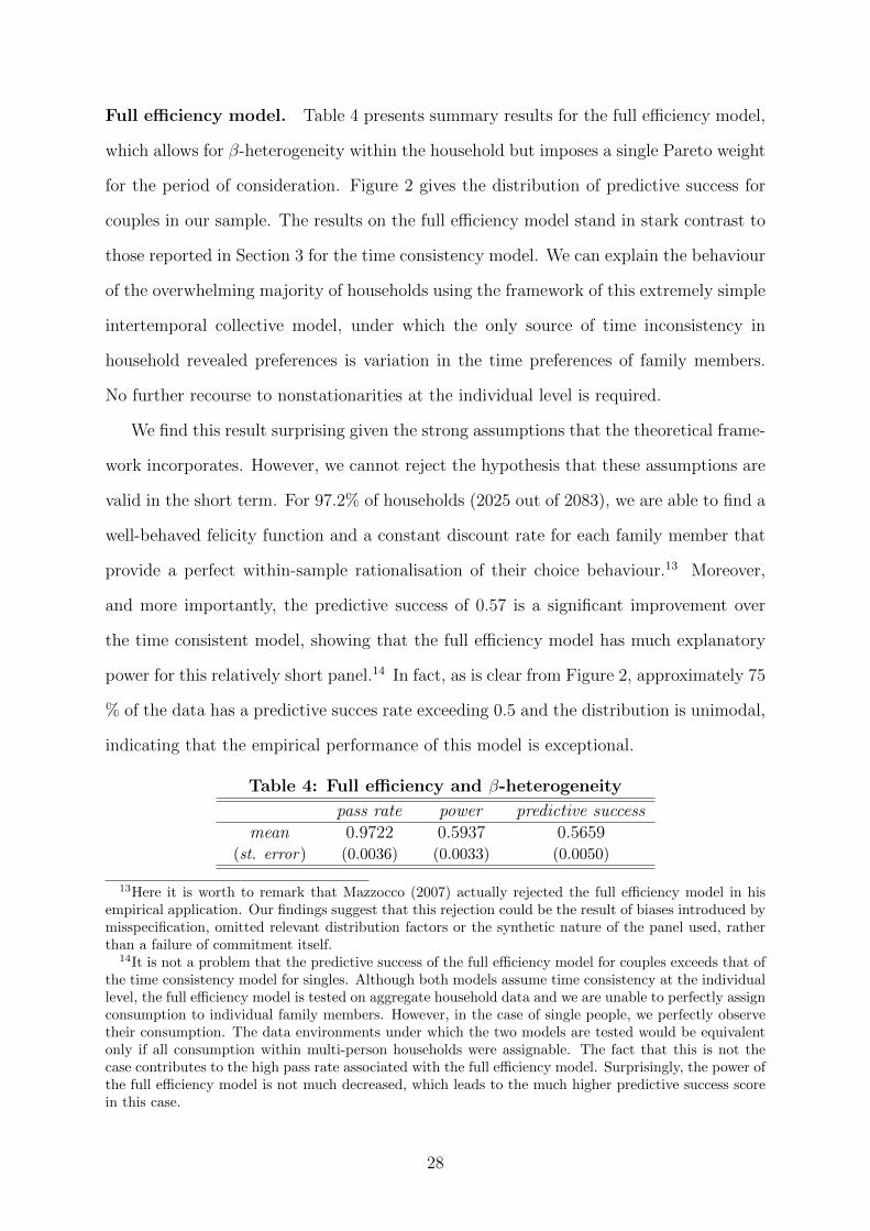
Full efficiency model. Table 4 presents summary results for the full efficiency model,
which allows for β-heterogeneity within the household but imposes a single Pareto weight
for the period of consideration. Figure 2 gives the distribution of predictive success for
couples in our sample. The results on the full efficiency model stand in stark contrast to
those reported in Section 3 for the time consistency model. We can explain the behaviour
of the overwhelming majority of households using the framework of this extremely simple
intertemporal collective model, under which the only source of time inconsistency in
household revealed preferences is variation in the time preferences of family members.
No further recourse to nonstationarities at the individual level is required.
We find this result surprising given the strong assumptions that the theoretical frame-
work incorporates. However, we cannot reject the hypothesis that these assumptions are
valid in the short term. For 97.2% of households (2025 out of 2083), we are able to find a
well-behaved felicity function and a constant discount rate for each family member that
provide a perfect within-sample rationalisation of their choice behaviour.13 Moreover,
and more importantly, the predictive success of 0.57 is a significant improvement over
the time consistent model, showing that the full efficiency model has much explanatory
power for this relatively short panel.14 In fact, as is clear from Figure 2, approximately 75
% of the data has a predictive succes rate exceeding 0.5 and the distribution is unimodal,
indicating that the empirical performance of this model is exceptional.
Table 4: Full efficiency and β-heterogeneity
pass rate power predictive successmean
(st. error)
0.9722(0.0036)
0.5937(0.0033)
0.5659(0.0050)
13Here it is worth to remark that Mazzocco (2007) actually rejected the full efficiency model in hisempirical application. Our findings suggest that this rejection could be the result of biases introduced bymisspecification, omitted relevant distribution factors or the synthetic nature of the panel used, ratherthan a failure of commitment itself.
14It is not a problem that the predictive success of the full efficiency model for couples exceeds that ofthe time consistency model for singles. Although both models assume time consistency at the individuallevel, the full efficiency model is tested on aggregate household data and we are unable to perfectly assignconsumption to individual family members. However, in the case of single people, we perfectly observetheir consumption. The data environments under which the two models are tested would be equivalentonly if all consumption within multi-person households were assignable. The fact that this is not thecase contributes to the high pass rate associated with the full efficiency model. Surprisingly, the power ofthe full efficiency model is not much decreased, which leads to the much higher predictive success scorein this case.
28

No-commitment model. Table 5 reports the results for the model that admits rene-
gotiation but assumes β-homogeneity. Unsurprisingly, allowing for more frequent rene-
gotiations of the Pareto weight is associated with an increase in the pass rate.15 For the
extreme scenario that allows innovations in the Pareto weight between any two consecu-
tive periods, the pass rate amounts to 98.4%, which is almost identical to the pass rate
of the full efficiency model. However, and importantly, once we correct for how demand-
ing the test is, by taking into account the discriminatory power, the average predictive
success of the no-commitment model with homogeneous discount rates falls below zero,
indicating that the model is not informative for household choice. As soon as we require
a stable Pareto weight over two periods or more, the pass rate drops steadily, and the
predictive success always remains negative and close to zero.
We conclude that accounting for the collective nature of household choice allows the
intertemporal behaviour of families in our sample to be explained using simple models that
assume constant discounting at the individual level. For the given data set, our results
provide particularly strong empirical support for a model which locates the primary
source of time inconsistent family behaviour with intrahousehold β-heterogeneity. The
full efficiency model seems plausible given the short time span of our sample.
Table 5: Renegotiation and β-homogeneity
renegotiations (max.) pass rate power predictive success
0mean
(st. error)0.1402
(0.0076)
0.8490(0.0008)
-0.0108(0.0082)
1mean
(st. error)0.6279
(0.0106)
0.3347(0.0019)
-0.0374(0.0104)
2mean
(st. error)0.9073
(0.0064)
0.0696(0.0008)
-0.0231(0.0063)
3mean
(st. error)0.9842
(0.0027)
0.0130(0.0002)
-0.0028(0.0027)
5.2 Time preference recovery
The analysis above suggests that the full efficiency model, which allows for time preference
heterogeneity, performs well for the data at hand. Given this implied importance of
15This is unsurprising since increasing the number of (possible) renegotiations generally obtains lessstringent rationalisability conditions.
29
discount rate heterogeneity in accounting for household consumption behaviour, we now
explore the nature of the theory-consistent set of household discount rates, and consider
whether the necessary degree of unobservable preference heterogeneity correlates with
observable family characteristics.
Minimum heterogeneity. For each household that can be rationalised by the full ef-
ficiency model, we recover the discount rates that make observed consumption behaviour
consistent with the rationalisability conditions in Theorem 2. One drawback of our re-
vealed preference methodology is that the identification of these discount rates is neces-
sarily weakened by the lack of structure our framework imposes on individual preferences
and the household choice problem. Our recovery problem is thus underdetermined and
preferences are only set identified in the sense of Manski (2007). We refer to this set of
potential time preferences as the set of “theory consistent discount rates”.
We deal with this non-uniqueness by reporting results for the minimal amount of
discount rate heterogeneity that is necessary to rationalise the household consumption
stream. To determine the minimum difference in household h’s discount factors, (βh,A −
βh,B), over the discount factor grid, we iterate the testing procedure by considering the
allowable grid points in a specific order. We initially set βh,A−βh,B = 0, which corresponds
to the time consistent model, and thus is rejected for about 86% of the households
in our sample. For the remaining households, we ask if behaviour can be rationalised
for βh,A − βh,B = 0.005, by testing for a non-empty set to the inequalities defined by
Theorem 2 with βh,A ∈ [1, 0.995, ..., 0.905] and βh,B = βh,A − 0.005. For the remaining
non-rationalisable households, the difference is then set at 0.01, and so on until the
maximum difference is reached when βh,A = 1 and βh,B = 0.90.
We are able to assume that βh,A ≥ βh,B without loss of generality because the data
set does not contain assignable goods, whose consumption can be tied to a particular
household member. Therefore, the revealed preference conditions for m = {A,B} are
fully symmetric. Sadly this implies that we cannot test for whether the husband or wife
is the more patient household member, and we choose not to make a prior assumption on
this dimension. If assignable information were available, analysis using our methodology
30

could be easily extended to address gender-related questions.
The distribution of the minimum discount factor heterogeneity for all 2025 rational-
isable is shown in Figure 3. Only limited heterogeneity is required to rationalise the
behaviour of most households. About three quarters of the households that are consis-
tent with Theorem 2 only require βA − βB ≤ 0.020 to rationalise their behaviour. The
kernel plot in Figure 3 confirms that the distribution of minimal heterogeneity shows a
high and relatively narrow peak for limited amounts of within-household heterogeneity
in time preferences. We also note that the maximum allowable heterogeneity level of 0.10
is observed only for a very small fraction of rationalisable households.
Appeal to observed heterogeneity. We investigate whether patterns in minimum
unobservable time preference heterogeneity (βh,A − βh,B) are related to observable het-
erogeneity via a simple regression of the log of the minimum discount rate distance on
recorded household characteristics.16 The ECPF contains information on a number of
household characteristics, including the age of each spouse, schooling and employment
status of the head, employment status of the wife (“wife working”), job skill level of both
spouses, presence and number of children in the household, and housing tenure. The
“husband skilled job” dummy equals 1 if the husband is a specialized worker but his wife
is not, with analogous interpretations for the “wife skilled job” and “both skilled job”
dummies. We also consider the level of the log of total consumption expenditures as
independent variables.
We note at the outset that the aim of this reduced form analysis is not to lay bare
structural relations between discount rate heterogeneity and household characteristics.
We mainly intend to conduct an -admittedly- fairly rudimentary exploratory exercise.
One significant drawback of our analysis is that we are unable to investigate gender
differences in time preferences because we lack assignable consumption information in
our sample. This makes it impossible to know the identity of members A and B without
16As we are interested in the direction of correlation between particular variables and the difference indiscount rates, rather than the precise magnitude of the coefficient, we consider the dependent variablelog(0.1 + βh,A − βh,B) to account for the skew in the distribution of differences, while keeping thosehouseholds who could be rationalised with βh,A = βh,B in our sample.
31

invoking additional heroic assumptions. Furthermore, it should be noted that we only
consider one element of the set of theory-consistent discount rates in our regression (that
giving rise to the minimal divergence between spousal discount rates). These factors help
to explain why the R-squared of our regression is very low.
Despite the limitations of our analysis, we are still able to provide some informal
evidence that relates our results to the recent literature on marriage matching and female
bargaining power. For example, Chiappori and Reny (2005) consider marriage matching
in the presence of heterogeneous risk preferences.17 In their model, marriage acts as
a device to share exogenous income risk. In their unique stable matching equilibrium,
there is negative assortative matching on the risk preferences, i.e. more risk averse men
will always be matched with less risk averse women. However, there is no reason to
expect negative assortative matching on time preferences. In related literature, match
quality is closely aligned to similarity in time preferences. For example, Schaner (2014)
classes couples as either “well” or “badly” matched purely on the basis of differences in
their elicited discount rates. Moreover, an individual’s level of patience (measured by
the discount factor) is likely to be correlated with other personal characteristics such
as education level. The couples in our sample have already self-selected into marriage,
presumably because of a high match quality, making it more likely that these couples
will also have similar time preferences, i.e. |βh,A − βh,B| will be small. Actually, our
empirical results seem to confirm this intuition, as they suggest that little intrahousehold
heterogeneity is required to rationalise the consumption behaviour in our sample. In fact,
this also makes that there is not much heterogeneity left to explain in our OLS regression.
However, as we discuss below, we do find some significant results that are noteworthy.
17In a related study, Dupuy and Galichon (2014) investigate the empirical relationship between sortingon the marriage market and individual risk attitudes in interaction with other personal characteristics.
32
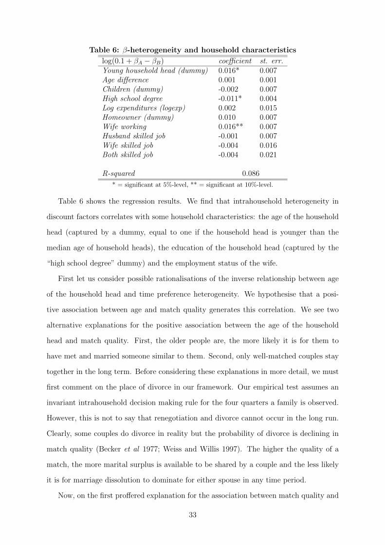
Table 6: β-heterogeneity and household characteristics
log(0.1 + βA − βB) coefficient st. err.Young household head (dummy) 0.016* 0.007Age difference 0.001 0.001Children (dummy) -0.002 0.007High school degree -0.011* 0.004Log expenditures (logexp) 0.002 0.015Homeowner (dummy) 0.010 0.007Wife working 0.016** 0.007Husband skilled job -0.001 0.007Wife skilled job -0.004 0.016Both skilled job -0.004 0.021
R-squared 0.086
* = significant at 5%-level, ** = significant at 10%-level.
Table 6 shows the regression results. We find that intrahousehold heterogeneity in
discount factors correlates with some household characteristics: the age of the household
head (captured by a dummy, equal to one if the household head is younger than the
median age of household heads), the education of the household head (captured by the
“high school degree” dummy) and the employment status of the wife.
First let us consider possible rationalisations of the inverse relationship between age
of the household head and time preference heterogeneity. We hypothesise that a posi-
tive association between age and match quality generates this correlation. We see two
alternative explanations for the positive association between the age of the household
head and match quality. First, the older people are, the more likely it is for them to
have met and married someone similar to them. Second, only well-matched couples stay
together in the long term. Before considering these explanations in more detail, we must
first comment on the place of divorce in our framework. Our empirical test assumes an
invariant intrahousehold decision making rule for the four quarters a family is observed.
However, this is not to say that renegotiation and divorce cannot occur in the long run.
Clearly, some couples do divorce in reality but the probability of divorce is declining in
match quality (Becker et al 1977; Weiss and Willis 1997). The higher the quality of a
match, the more marital surplus is available to be shared by a couple and the less likely
it is for marriage dissolution to dominate for either spouse in any time period.
Now, on the first proffered explanation for the association between match quality and
33

age, consider the search process leading to marriage. If this process is costly, individuals
will accept imperfect matches even if it is known that differences in time preferences
will create inefficiencies in the new household (see Burdett and Coles (1999) for a for-
mal framework). Over time, if some search continues during marriage, individuals will
continue to acquire new information on other potential matches. If a spouse meets a
high enough quality match, it can be worth dissolving an existing marriage to take up a
new opportunity. The older someone is, the longer they will have been a participant in
the marriage market and therefore, the more likely it is that they will have met someone
similar to themselves and thus be a member of a “high quality” match. In this way, costly
search can create a negative association between age and discount rate heterogeneity.
Alternatively, on the second explanation, it is not unreasonable to assume that older
couples have been married longer. Some model match quality as an experience good
(Nelson 1970; Jovanovic 1979; Weiss and Willis 1997; Chiappori and Weiss 2006). In
contrast to the above, these explanations assume that one cannot perfectly assess the
suitability of a potential mate until marriage occurs and a match is experienced. Given
that young couples have lower marriage experience, one can expect a greater variation in
match quality (i.e. heterogeneity in discount rates) amongst this group, as these couples
are still assessing the degree to which they are suited and not all poor matches will have
been terminated. However, only well suited couples will remain married for a long period
of time, again creating a negative association between the age of a couple and discount
rate heterogeneity.
The household head having a high school degree and the wife not working are also
associated with smaller heterogeneity in time preferences. If one is willing to make the
strong assumption that the husband has a lower discount factor than the wife, then we
can label the wife as member A and the husband as B, since our dependent variable
βh,A − βh,B is defined to be (weakly) positive.18 Additionally, one may posit that more
patient individuals are more likely to invest more in their education (i.e. to have a high
18In the literature, it is often found that males are less patient than females, supporting our assumption;see for example Kirby and Maracovic (1996), Warner and Pleeter (2001), Ubfal (2013), and Dittrich andLeipold (2014). This might be the case because men have a shorter life expectancy than women, makingthem less patient on average, all else equal.
34

school degree) and also therefore more likely to be employed later in life. Hence, all else
equal, a husband (defined to be the household head for our sample) with a high school
degree will have a higher patience level βh,B, leading to a lower level of time preference
heterogeneity. Similarly, a working wife will have a higher βh,A, causing a higher level of
time preference heterogeneity.
As a different explanation, working wives may have more bargaining power or better
outside options, which makes it more likely that their participation constraint becomes
binding at some point, so creating a need to renegotiate the intra-household Pareto
weights. As a result, because our full efficiency model excludes such renegotiation, it
might be harder to satisfy its empirical restrictions and, thus, a larger set of grid points
(βh,A, βh,B) needs to be considered in order to rationalise the data. Since our dependent
variable (βh,A − βh,B) is defined as the minimum required discount rate heterogeneity
needed to explain the data, the positive coefficient on the “working wife” dummy would
then be a mechanical result of our testing procedure.
Follow-up research, potentially using richer data sets, may focus on better explaining
these patterns. For example, as indicated above, data sets that include information on
assignable goods can allow for more robust identification of gender-specific effects, which
seem to be relevant here.
6 Conclusion
We have provided a revealed preference analysis of time inconsistencies in household
consumption. Adopting a collective perspective, we focused on rationalising these incon-
sistencies as the product of individual time preference heterogeneity and renegotiation
within the household unit. An empirical application to a Spanish consumption panel
highlights that an explicit recognition of the collective nature of choice allows us to ratio-
nalise the vast majority of time inconsistent household behaviour. Almost all observed
household behaviour turns out to be consistent with a simple model that assumes perfect
intrahousehold commitment (i.e. no renegotiation) in the one-year period under con-
35

sideration together with exponential discounting at the individual level, so long as time
preferences heterogeneity is allowed for.
We have also shown that revealed preference restrictions can be fruitfully applied to
recover individual time preferences. One can then relate these results to specific indi-
vidual or household characteristics. For example, for our application we found that the
intrahousehold heterogeneity in discount factors correlates with the age and educational
level of the household head and the wife’s employment status. This application demon-
strates the potential usefulness of revealed preference methodology to address this type
of questions in an effective manner. It is our belief that richer household data sets (e.g.
including assignable goods and more information on observable characteristics) may yield
additional and more refined insights. In principle, for long enough panels with detailed
information, our framework also enables one to investigate how variation in specific (indi-
vidual and household) characteristics relates to patterns of intrahousehold renegotiation.
References
[1] Abi Adams (2011), Household Intertemporal Choice: A Nonparametric Characteri-sation, Mimeo.
[2] Sydney Afriat (1967), The Construction of Utility Functions from Expenditure Data,International Economic Review, 8.1 p67-77.
[3] Steffen Andersen, Glenn W. Harrison, Arne Risa Hole, Morten Lau, E. ElisabetRutstrom (2012), Non-linear Mixed Logit, Theory and Decision, 73(1), p77-96.
[4] James Andreoni and Charles Sprenger (2012), Estimating Time Preferences fromConvex Budget Sets, American Economic Review, 102(7), p3333-3356.
[5] George-Mario Angeletos, David Laibson, Andrea Repetto, Jeremy Tobacman andStephen Weinberg (2001), The Hyperbolic Consumption Model: Calibration, Simu-lation and Empirical Evaluation, Journal of Economic Perspectives, 15.3 p47-68.
[6] Timothy K. Beatty and Ian Crawford (2011), How Demanding is the Revealed Pref-erence Approach to Demand?, American Economic Review, 101, p2782-2795.
[7] Gary Becker (1962), Irrational Behavior and Economic Theory, Journal of PoliticalEconomy, 70, p1-13.
[8] Gary Becker, Elizabeth Landes, Robert Michael (1977), An Economic Analysis ofMarital Instability, Journal of Political Economy, 85, p1141-1187.
[9] Stephen G. Bronars (1987), The Power of Nonparametric Tests of Preference Maxi-mization, Econometrica, 55, p693-698.
36

[10] Martin Browning (1989), A Nonparametric Test of the Life-Cycle Rational Expec-tations Hypothesis, International Economic Review, 30.4 p979-992.
[11] Martin Browning, Francois Bourguignon, Pierre-Andre Chiappori, Valerie Lechene(1994). Income and Outcomes: A Structural Model of Intrahousehold Allocation,Journal of Political Economy, 102, p1067-96.
[12] Martin Browning and Pierre Andre Chiappori (1998), Efficienct Intra-householdAllocations: A General Characterisation and Empirical Tests, Econometrica, 66.6p1241-1278.
[13] Kenneth Burdett and Melvyn Coles (1999), Long Term Partnership Formation: Mar-riage and Employment, The Economic Journal, 109, p307-334.
[14] Laurens Cherchye, Bram De Rock and Frederic Vermeulen (2007), The CollectiveModel of Household Consumption: A Nonparametric Characterization, Economet-rica, 75.2 p553-574.
[15] Laurens Cherchye, Bram De Rock and Frederic Vermeulen (2009), Opening theBlack Box of Intra-household Decision-making: Theory and Nonparametric Empiri-cal Tests of General Collective Consumption Models, Journal of Political Economy,117, p1074-1104.
[16] Pierre-Andre Chiappori (1988), Rational Household Labor Supply, Econometrica,56, p63-89.
[17] Pierre-Andre Chiappori (1992), Collective Labor Supply and Welfare, Journal ofPolitical Economy, 100, p437-67.
[18] Pierre-Andre Chiappori and Philip J. Reny (2005), Matching to Share Risk, Mimeo.
[19] Pierre-Andre Chiappori amd Yoram Weiss (2006), Divorce, Remarriage and Welfare:A General Equilibrium Approach, Journal of the European Economic Association4.2/3, Papers and Proceedings of the Twentieth Annual Congress of the EuropeanEconomic Association p415-426.
[20] James Choi, David Laibson, Brigitte Madrian and Andrew Metrick (2001), For Bet-ter or for Worse: Default Effects and 401(k) Savings Behavior, In Perspectives onthe Economics of Ageing, edited by David Wise, University of Chicago Press forNBER.
[21] Ian Crawford (2010), Habits Revealed, Review of Economic Studies, 77.4 p1382-1402.
[22] Stefano DellaVigna and Ulrike Malmendier (2006), Paying Not To Go To The Gym,The American Economic Review, 96, p694-719.
[23] W.E. Diewert (1973), Afriat and Revealed Preference Theory, The Review of Eco-nomic Studies, 40.3 p419-425.
[24] Marcus Dittrich and Kristina Leipold (2014), Gender Differences in Time Prefer-ences, Economics Letters, 122 p413-415.
37

[25] Thomas Dohman, Armin Falk, David Huffman, Uwe Sunde (2012), InterpretingTime Horizon Effects in Inter-Temporal Choice, CESifo Working Paper No. 3750.
[26] Arnaud Dupuy and Alfred Galichon (2014), Personality Traits and the MarriageMarket, The Journal of Political Economy, forthcoming.
[27] Martin S. Feldstein (1964), The Social Time Preference Discount Rate in Cost Ben-efitt Analysis, The Economic Journal, 74, p360-379.
[28] Shane Frederick, George Loewenstein, Ted O’Donoghue (2002), Time Discountingand Time Preference: A Critical Review, Journal of Economic Literature, Vol 40,No. 2, 351-401.
[29] Jonathan Gruber and Botond Koszegi (2000), Is Addiction ‘Rational?’ Theory andEvidence, Quarterly Journal of Economics, 116, p1261-1305.
[30] Matthew Jackson and Leeat Yariv (2012), Collective Dynamic Choice: The Necessityof Time Inconsistency, Mimeo.
[31] Boyan Jovanovic (1979), Job Matching and the Theory of Turnover, Journal ofPolitical Economy, 87.5 Part 1 p972-990.
[32] Kris. N. Kirby and Nino M. Marakovic (1996), Delay-discounting Probabilistic Re-wards: Rates decrease as amounts increase, Psychonomic Bulletin and Review, 3(1),100-104.
[33] Tjalling Koopmans (1960), Stationary Ordinal Utility and Impatience, Economet-rica, 28, p287-309.
[34] David Laibson (1997), Golden Eggs and Hyperbolic Discounting, Quarterly Journalof Economics, 112, p443-477.
[35] David Laibson (1998), Life-Cycle Consumption and Hyperbolic Discount Functions,European Economic Review, 42, p861-871.
[36] Albert Marcet and Ramon Marimon (1998), Recursive Contracts, Manuscript, Uni-versitat Pompeu Fabra.
[37] Stephen Marglin (1963), The Social Rate of Discount and The Optimal Rate ofInvestment, The Quarterly Journal of Economics, 77.1, p95-111.
[38] Charles Manski (2007), Identification for Prediction and Decision, Cambridge, MA:Harvard University Press.
[39] Maurizio Mazzocco (2007), Household Intertemporal Behaviour: A Collective Char-acterization and a Test of Commitment, Review of Economic Studies, 74.3 p857-895.
[40] Phillip Nelson (1970), Information and Consumer Behavior, Journal of PoliticalEconomy, 78.2 p311-329.
[41] Ted O’Donoghue and Matthew Rabin (1999), Doing It Now or Later, AmericanEconomic Review, 89.1 p103-124.
38

[42] Ted O’Donoghue and Matthew Rabin (2001), Choice and Procrastination, QuarterlyJournal of Economics, 116.1 p121-160.
[43] Karl Popper (1959), The Logic of Scientific Discovery, London: Hutchinson andCompany.
[44] Paul Samuelson (1937), A Note on the Measurement of Utility, Review of EconomicStudies, 4, p155-161.
[45] Simone G. Schaner (2014), Do Opposites Detract? Intrahousehold Preference Het-erogeneity and Inefficient Strategic Savings, American Economic Journal: AppliedEconomics, forthcoming.
[46] Reinhard Selten (1991), Properties of a Measure of Predictive Success, MathematicalSocial Sciences, 21, p153-167.
[47] Avner Shaked and John Sutton (1984), Involuntary Unemployment as a PerfectEquilibrium in a Bargaining Model, Econometrica, 52.6 p1351-1364.
[48] Richard Thaler and Shlomo Benartzi (2004), Save More Tomorrow: Using BehavioralEconomics to Increase Employee Saving, Journal of Political Economy, 112. 1 p164-187.
[49] Diego Ubfal (2013), How General Are Time Preferences? Eliciting Good-SpecificDiscount Rates, Working Papers 473, Bocconi University.
[50] Hal Varian (1982), The Nonparametric Approach to Demand Analysis, Economet-rica, 50, p945-973.
[51] Hal Varian (1985), Nonparametric Analysis of Optimizing Behavior with Measure-ment Error, Journal of Econometrics, 30, p445-458.
[52] John T. Warner and Saul Pleeter (2001), The Personal Discount Rate: EvidenceFrom Military Downsizing Programs, American Economic Review, 91(1), p33-53.
[53] Yoram Weiss and Robert Willis (1997), Match Quality, New Information and MartialDissolution, Journal of Labor Economics, 15.1 Part 2: Essays in Honor of YoramBen-Porath p293-329.
[54] Stephane Zuber (2011), The Aggregation of Preferences: Can We Ignore the Past?,Theory and Decision, 70, p367-384.
Appendix A: Proofs
This appendix gives the proofs of our Theorems 1-3.
39

Proof of Theorem 1
(Necessity) Suppose the set of observations Sh can be rationalised by the.time consis-
tency model. Let η denote the Lagrange multiplier associated with the household budget
constraint. We get the following first order constraints for the household optimisation
problem (with∂uh(qh,At ,qh,Bt ,Qh
t )
∂qh,mt(m ∈ {A,B}) and
∂uh(qh,At ,qh,Bt ,Qht )
∂Qht
the subgradients for the
function uh at (qh,At ,qh,Bt ,Qht )):
βt−1h
∂uh(qh,At ,qh,Bt ,Qht )
∂qh,mt≤ ηpt (m ∈ {A,B}) and
βt−1h
∂uh(qh,At ,qh,Bt ,Qht )
∂Qht
≤ ηPt.
Under concavity of the function uh, we have
uh(qh,As ,qh,Bs ,Qhs )− uh(q
h,At ,qh,Bt ,Qh
t ) ≤
(∂uh(qh,At ,qh,Bt ,Qh
t )
∂qh,At
)′(qh,As − qh,At ) +(
∂uh(qh,At ,qh,Bt ,Qht )
∂qh,Bt
)′(qh,Bs − qh,Bt ) +(
∂uh(qh,At ,qh,Bt ,Qht )
∂Qht
)′(Qh
s −Qht ).
Combining the different inequalities leads to
uh(qh,As ,qh,Bs ,Qhs )− uh(q
h,At ,qh,Bt ,Qh
t ) ≤η
βt−1h
[p′t(q
hs − qht ) + P′t(Q
hs −Qh
t )].
By using uh(qh,As ,qh,Bs ,Qhs )
η= uhs , we obtain the inequalities in Theorem 1.
(Sufficiency) Suppose the inequalities in Theorem 1 hold. Then, define the following
felicity function:
uh(xA,xB,X) = mins
(uhs +
1
βs−1h
[p′s(xA − qh,As ) + p′s(x
B − qh,Bs ) + P′s(X−Qhs )]
).
Using a straightforwardly similar argument as Varian (1982), we can derive uh(qh,At ,qh,Bt ,Qht ) =
uht .
40

Consider any consumption plan {xAt ,xBt ,Xt}t∈T such that
∑t∈T
[p′t(x
At − qh,At ) + p′t(x
Bt − qh,Bt ) + P′t(Xt −Qh
t )]≤ 0,
i.e. the consumption plan {xAt ,xBt ,Xt}t∈T is affordable given the outlay associated with
{qh,At ,qh,Bt ,Qht }t∈T . Then, we need to show that
∑t∈T
βt−1h uh(xAt ,x
Bt ,Xt) ≤
∑t∈T
βt−1h uh(qh,At ,qh,Bt ,Qh
t ).
Using the utility function defined above, we obtain
∑t∈T
βt−1h uh(xAt ,x
Bt ,Xt)
≤∑t∈T
βt−1h
(uht +
1
βt−1h
[p′t(xAt − qh,At ) + p′t(x
Bt − qh,Bt ) + P′t(Xt −Qh
t )]
)=
∑t∈T
βt−1h uht +
∑t∈T
[p′t(xAt − qh,At ) + p′t(x
Bt − qh,Bt ) + P′t(Xt −Qh
t )]
≤∑t∈T
βt−1h uht ,
so that uh(qh,At ,qh,Bt ,Qht ) = uht gives the wanted conclusion.
Proof of Theorem 2
(Necessity) Suppose the set of observations Sh can be rationalised by the full efficiency
model. Let η denote the Lagrange multiplier associated with the household budget con-
straint. We get the following first order constraints (with∂uh,m(qh,mt ,Qh
t )
∂qh,mtand
∂uh,m(qh,mt ,Qht )
∂Qht
(m ∈ {A,B}) the subgradients for the function uh,m at bundle (qh,mt ,Qht )):
βt−1h,A
∂uh,A(qh,At ,Qht )
∂qh,At≤ ηpt,
ωhβt−1h,B
∂uh,B(qh,Bt ,Qht )
∂qh,Bt≤ ηpt,
βt−1h,A
∂uh,A(qh,At ,Qht )
∂Qht
+ ωhβt−1h,B
∂uh,B(qh,Bt ,Qht )
∂Qht
≤ ηPt.
41

Under concavity of each felicity functions uh,m, we have
uh,m(qh,ms ,Qhs )−uh,m(qh,mt ,Qh
t ) ≤
(∂uh,m(qh,mt ,Qh
t )
∂qh,mt
)′(qh,ms −qh,mt )+
(∂uh,m(qh,mt ,Qh
t )
∂Qht
)′(Qh
s−Qht ).
Now define, for each t ∈ T,
λh,A = η, λh,B =η
ωh,
Ph,At =
βt−1h,A
λh,A∂uh,A(qh,At ,Qh
t )
∂Qht
,
Ph,Bt = Pt −Ph,A
t .
Combination yields
uh,m(qh,ms ,Qhs )− uh,m(qh,mt ,Qh
t ) ≤λh,m
βt−1h,m
p′t(qh,ms − qh,mt ) +
λh,m
βt−1h,m
(Ph,mt )′(Qh
s −Qht ).
By using uh,m(qms ,Qs)/λh,m = uh,ms , we obtain the inequalities in Theorem 2.
(Sufficiency) Suppose the inequalities in Theorem 2 hold. Then, define the following
felicity function for each member m ∈ {A,B}:
uh,m(xm,X) = mins
(uh,ms +
1
βs−1h,m
[p′s(xm − qh,ms ) + Ph,m′
s (X−Qhs )]
).
Using a straightforwardly similar argument as Varian (1982), we can derive uh,m(qh,mt ,Qht ) =
uh,mt .
Consider any consumption plan {xAt ,xBt ,Xt}t∈T such that
∑t∈T
[p′t(x
At − qh,At ) + p′t(x
Bt − qh,Bt ) + P′t(Xt −Qh
t )]≤ 0,
i.e. the consumption plan {xAt ,xBt ,Xt}t∈T is affordable given the outlay associated with
42

{qh,At ,qh,Bt ,Qht }t∈T . Then, for ωA = 1 and ωB = ωh we need to show that
∑m∈{A,B}
∑t∈T
ωmβt−1h,mu
h,m(xmt ,Xt) ≤∑
m∈{A,B}
∑t∈T
ωmβt−1h,mu
h,m(qh,mt ,Qht ).
Without losing generality, we can assume ωm = 1. As such, we obtain
∑m∈{A,B}
∑t∈T
ωmβt−1h,mu
h,m(xmt ,Xt)
≤∑
m∈{A,B}
∑t∈T
ωmβt−1h,m
(uh,mt +
1
βt−1h,m
[p′t(xmt − qh,mt ) + Ph,m′
t (Xt −Qht )]
)=
∑m∈{A,B}
∑t∈T
ωmβt−1h,mu
h,mt +
∑m∈{A,B}
∑t∈T
[p′t(xmt − qh,mt ) + Ph,m′
t (Xt −Qht )]
≤∑
m∈{A,B}
∑t∈T
ωmβt−1h,mu
h,mt ,
so that uh,m(qh,mt ,Qht ) = uh,mt gives the wanted conclusion.
Proof of Theorem 3
The result uses that, for a given partition T, consistency with the no-commitment model
requires that, for each subset Tτ (τ ∈ {1, ...,Υ}), that the corresponding subset of ob-
servations {qht ,Qht ; pt,Pt}t∈Tτ can be rationalized by the full efficiency model. Then, the
result follows directly from Theorem 2.
Appendix B: Summary statistics
The following table provides summary statics of the data we use in our empirical applica-
tion. For the different (public and private) goods it gives average expenditure shares and
discounted prices over all observations (i.e. 4 observations for 2083 households), together
with the corresponding standard deviations.
43

Private goodsMean sharest. dev:
overallbetweenwithin
Mean pricest. dev:
overallbetweenwithin
Food and non-alcoholic drinks
0.45640.18930.14990.1156
1.43300.26840.25000.9783
Clothing and footwear
0.16320.13500.08090.1081
1.45460.30550.28450.1086
Transportation
0.04610.07570.04580.0604
1.56470.44060.39610.1930
Leisure (cinema, theatre, clubs for sport)
0.05690.07340.05010.0536
1.44170.28780.25980.1239
Personal services
0.02540.04410.02640.0353
1.43590.29640.26000.1425
Restaurants and bars
0.13460.13030.10010.0834
1.55110.37700.34730.1469
Public goods
Mean sharest. dev:overallbetweenwithin
Mean pricest. dev:
overallbetweenwithin
Home Services (heating, water and furniture repair)
0.04550.06580.05470.0366
1.38150.25110.23040.0999
Petrol
0.07190.07860.05750.0536
1.02220.11370.11060.0263
The following table records summary statistics on household characteristics considered
in the course of our empirical exploration of time preference heterogeneity.
44

Characteristic Mean St. Dev.Average age of couple 35.8 8.97Husband age 37.5 9.25Wife age 34.2 8.91High school degree dummy 0.57 0.49Children dummy 0.79 0.41Couple + 1 child 0.27 0.46Couple + 2 children 0.42 0.49Couple + 3 or more children 0.10 0.30Home owner dummy 0.72 0.45Wife working dummy 0.36 0.48Husband skilled job dummy 0.30 0.46Wife skilled job dummy 0.08 0.28Both skilled job dummy 0.05 0.21
45