construction site pedestrian simulation with moving obstacles

September 6, 2016 15:1 RPS/Trim Size: 24cm x 17cm for Proceedings/Edited Book fbi16-paper

Construction site pedestrian simulation with moving obstacles

Giovanni Filomeno1, Ingrid I. Romero1 , Ricardo L. Vásquez1, Daniel H.Biedermann1, Maximilian Bügler1

1 Lehrstuhl für Computergestützte Modellierung und Simulation,Technical University Munich,

Arcisstraße 21, 80333 München, Germany.E-mail: [email protected]

The simulation of pedestrian movement in a dynamic environment is an important challenge inengineering safety simulation. One application is pedestrian dynamics for construction sites.The responsible management must ensure the safety of their workers on the construction site.In recent years, the use of computer simulations has become an important tool for designingsafe pedestrian patterns. In this paper we describe a simulation of workers in a constructionenvironment with moving obstacles. The simulation models the movements of the workersand obstacles in a 2D plane, with all the moving obstacles such as bulldozers, excavators andother heavy machines having a safety area around them. This safety area approximates thetendency of humans to avoid moving objects more so than static ones. Our method is based ona combination of repelling and attractive forces. The sum of all the forces shapes the path thata pedestrian will take.

Keywords: Pedestrian dynamics simulations, moving obstacles avoidance, potential fields.

1. Introduction

The safety of workers on large construction sites is a complex and important topic in thefield of civil engineering. To prevent worker injury, the construction management must haveinformation about the movements of their workers on the construction site. One way to obtainthis information is through pedestrian dynamics simulation. Pedestrian dynamics simulationsare normally modeled with the help of three independent and interacting layers (Hoogendorn& Bovy , 2004): strategic, tactical and operational.

The strategic layer determines which destination a pedestrian is heading to next. For everyday purposes, this decision process can be carried out by cognitive decision models (Kielar &Borrmann , 2016). However, in the case of construction workers, the different places wherethey have to work is predefined by the daily work schedule. Thus our simulation uses thisschedule to define the sequential order in which a worker goes from one place to another (seeSection 3.3).

The tactical layer provides the route along which the pedestrian will move in order to reachthe final point. The literature covers a range of tactical models, from the easiest “shortest path”,e.g. the algorithm A* (Kadry et al. , 2012), to more complex approaches taking into accountpsychological knowledge (Kielar et al. , 2016). In our simulation model, the tactical layerconsists of an attractive force which acts all over the construction site (see Section 3.3) anddetermine the destination of the worker.

The operational layer models actual movement. For example, in our case the operational

1


28. Forum Bauinformatik 201619.–21. September 2016, Leibniz Universität Hannover

layer ensures that the pedestrian will not collide with other pedestrians or obstacles. Moreoverthe operational layer describes the repulsive forces which act on obstacles, either fixed ormoving.

Models of Pedestrian dynamics can be simulated on different space-dependent scales: thethree most common are macroscopic, mesoscopic and microscopic. The difference between themacroscopic and non-macroscopic approaches is that macroscopic models only use cumulativeparameters (e.g. pedestrian densities), whereas non-macroscopic models consider pedestriansas individual and discrete agents. The most common macroscopic model is the LWR-model(Lighthill & Whitham , 1955; Richards , 1956; Colombo & Rosini , 2005). There are non-macroscopic models that can simulate individual pedestrians: microscopic models, such associal force models (Helbing & Molnár , 1995), and mesoscopic cellular automata models(Blue & Adler , 1998). Additionally, hybrid models can combine models from different spatialscales to lower the overall computational cost (Biedermann et al. , 2014, 2016; Ijaz et al. ,2015).

The content of this paper is divided as follows. The second section describes the backgroundfor our solution and discusses the advantages and disadvantages of other approaches. In thethird section there is a detailed explanation of the potential field algorithm applied in oursolution. In Section 4, we describe the implementation and the main characteristics of theapplication developed for this project. The fifth section presents the conclusions and futuresteps for this project.

2. Related work

For this work, defining and describing pedestrians in a dynamic environment, the constructionsite was described using social force model (Helbing & Molnár , 1995) and obstacle avoidancealgorithms. All obstacles are modeled by their shape and define an area that should be avoidedby pedestrians. This approach allows us to define interest points for the pedestrians, and createthe construction site as a group of zones where the pedestrians can move safely. For the threealgorithms that were studied, the following assumptions hold:

• The obstacles can have arbitrary shapes.

• The working space is considered in 2D.

• Every single pedestrian has to reach a final point.

These algorithms are briefly described in the next section. The “Visibility graph” algorithm(Huang & Chung , 2004) defines the obstacles as polygons. The goal is to find the shortest pathto the final point. The "Visibility graph" is an indirect method which consist of connecting thetwo main points, in our case this means starting and final points, with all the corners of theobstacles with straight lines (See Figure 1).

A requirement of the line is that it must not pass through the internal area of the polygon.Considering this, a network that connects all the corners of the obstacles and the final and initialpoints is created. Finding and choosing the shortest path is now only a problem of comparison.After that, the pedestrian can move following the line of decided path. Figure 1 demonstrateshow the algorithm works. The pedestrian moves from the starting point to the corners and thencontinue from the corners to the end point.

The disadvantages of this method are that all objects have to be described by polygons,

2



Fig. 1. Visibility Graph example

that makes it more difficult to work with continuous shapes. To find the shortest path, all thepossible paths must be compared, which leads to a higher computational effort compared withother methods.

Another approach is the so called bug algorithm (Yufka & Parlaktuna , 2009), which mimicsthe behavior of insects, such as ants. It can be divided into two steps:

1- Draw the shortest line that connect the starting point and the final one.

2- The pedestrian must move along the line until one of the following two case is met :

2.1- If the pedestrian reaches the final point then stop.2.2- If the pedestrian touches an obstacle, he stops there, follows the shape of the obstacles

until he reaches the shortest line again. Return to step 2 (See Figure 2).

Fig. 2. Bug Algorithm example

This approach works with any shape of the obstacles, however, it requires that the pedestriangets close to the obstacle and the path is not smooth.

During our research for the best algorithm to implement we discarded the visibility graphand bug algorithm because of the inconveniences of each one:

• In the bug algorithm, the pedestrians have to reach the obstacles in order to avoid them, butthis is unacceptable since they should start avoiding the obstacles before reaching them.

• In the case of the visibility graph method, the path may be computed avoiding the edgesof the obstacles, however, this method is not very efficient to work with dynamic updating

3



of the elements in the simulation.

3. Simulation model

3.1. Strategic layer

The strategic layer is created because all the workers have a work schedule. To model this,we create arrays for each pedestrian that contain their destinations one needs to reach duringthe simulation. Each destination represents a place where the worker has to do a task e.g.building a wall, collecting material, etc. Thus, the worker waits for some time at each of thesedestinations. This represents that the worker is performing some task in that place.

Since the workflow of the worker is linear, there is always only one goal for each point intime. When the current goal is accomplished the next one is adapted as the new goal. Thisprocess continues until the pedestrian gets to all the destinations in the array.

3.2. Tactical and operational layer

In this approach the tactical and operational layer are composed of the attractive and repulsiveforces of the next destination a pedestrian is heading to.

3.3. Algorithm approach

As an alternative to the approaches described in Section 2, one of our requirements is analgorithm which can avoid obstacles, for example, the movements of vehicles on a constructionsite.

The approach relies on a model of the construction site having two artificial fields: attractionand repulsion. Our approach thus follows the idea of social force (Helbing & Molnár ,1995). Our approach is a representation of physical phenomena, where the target points canbe modeled as sinks and the obstacles as surfaces with high elevation. The pedestrian can thenbe modeled as a free object that will move around according to the sum of the attractive andrepulsive forces (see Figure 3c).

As described above, the destination is the source of the attractive field, acting all over thefield with a constant value (see Figure 3a). When the pedestrian is far away or very close to thegoal, the strength of the field will decrease. In contrast, all the obstacles will create a repulsivefield around them with in a limited range. When the pedestrian is inside the effective area ofthe obstacle’s field, the force will increase as the pedestrian gets closer (see Figure 3b).

4



a) b) c)

Fig. 3. a) Representation of attractive force, b) Representation of repulsive force, c) The 3d representa-tion of repulsive (peak values) and attractive (dip values) forces

The governing equations for the attractive and repulsive fields are as follows:Equations for the attraction force

U = Pg − Pp (1)

U =U

‖U‖= a vector of unit length from the pedestrian to the goal (2)

If the pedestrian is inside the goal zone:

FA = αU (3)

If the pedestrian is far from the goal zone:

FA = βU (4)

where:

Pg= Position of the Goal

Pp= Position of the Pedestrian

FA= Attraction Force

r= Radius of the goal zone

β= Magnitude of the force for all the field

α =β

r= Constant to decrease the force inside the goal zone

Equations for the repulsive force

V = Pp − Po (5)

V =V

‖V ‖vector of unit length from the obstacle to the pedestrian (6)

If the pedestrian is inside of the restricted area of the obstacle:

FR = SV (7)

5



If the pedestrian is inside of the effective area ρ of the obstacle:

FR = γ(ro − ‖V ‖)U (8)

where :

ro=Effect area of obstacle

S= Speed of the obstacle

P0= Position of the Obstacles

PP = Position of Pedestrian

FR= Repulsive Force

γ= Magnitude of the repulsive force

To apply the previous equations, it is necessary to know whether the pedestrian is inside theeffective area of an obstacle, which, for polygons is calculated by the following method: theobstacles are defined by a set of points given in counter clockwise direction. For each edge ofthe obstacle the equation of the line is defined from two points as follows:

P1 = (x1, y1) (9)

P2 = (x2, y2) (10)

Ax+By + C = 0 (11)

where

A = y2 − y1 (12)

B = x1 − x2 (13)

C = y1x2 − x1y2 (14)

(15)

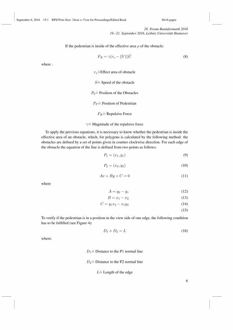
To verify if the pedestrian is in a position in the view side of one edge, the following conditionhas to be fulfilled (see Figure 4):

D1 +D2 = L (16)

where:

D1= Distance to the P1 normal line

D2= Distance to the P2 normal line

L= Length of the edge

6



Fig. 4. Method for verifing the presence of pedestrians near an obstacle

Once the pedestrian is confirmed to be in the range of one edge, then the distance to theedge, D, has to be checked to verify that it is smaller than the effective area for that obstacle:

D =Ax+By + C

L(17)

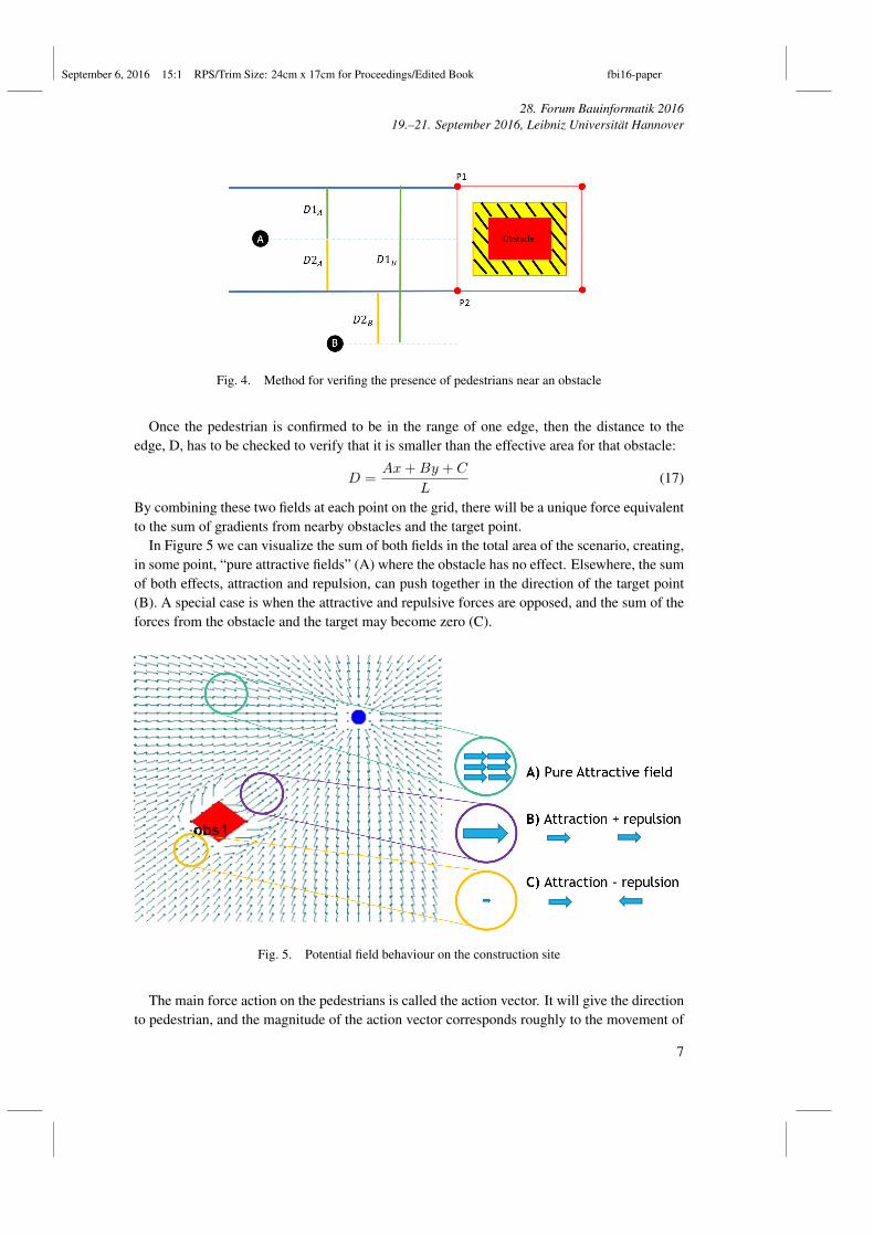
By combining these two fields at each point on the grid, there will be a unique force equivalentto the sum of gradients from nearby obstacles and the target point.

In Figure 5 we can visualize the sum of both fields in the total area of the scenario, creating,in some point, “pure attractive fields” (A) where the obstacle has no effect. Elsewhere, the sumof both effects, attraction and repulsion, can push together in the direction of the target point(B). A special case is when the attractive and repulsive forces are opposed, and the sum of theforces from the obstacle and the target may become zero (C).

Fig. 5. Potential field behaviour on the construction site

The main force action on the pedestrians is called the action vector. It will give the directionto pedestrian, and the magnitude of the action vector corresponds roughly to the movement of

7



the pedestrian (see Figure 6).

Fig. 6. History of the trajectory followed by the pedestrians

3.4. Local Zero

One important problem is the local zero or “local minima” (Koren & Borenstein , 1991), wherethe attracting and repulsing fields have the same values but in opposite directions. In thesecases the pedestrian will get stuck in that point. To avoid the creation of convergence points outof the desired target, two additional potential fields may be added to the previous formulationto take the pedestrian out of the local minima:

• Rotational field around the obstacles: this option will help us to avoid the local minimum,breaks the symmetry and guides the pedestrian around groups of obstacles when they arein movement (see Figure 7a).

• Random field: the creation of small random forces around the obstacle gets the pedestrianunstuck and avoids some local minimum (see Figure 7b).

a) b)

Fig. 7. a) Rotational field example, b) Random field example

3.5. Moving Obstacles

In this section, the representation of all the obstacles in the simulation is described in detail. Asmentioned before, the main goal is to obtain results from a dynamic simulation, which meansthat the environment consists of moving obstacles with different shapes that should be avoidedby the pedestrians. The moving obstacles represent the machines in the construction site, suchas excavators, bulldozers and other heavy machines. The different types of obstacles available

8



in the simulation are:

• Obstacles of arbitrary shapes with fixed path and a waiting time at some points

• Moving obstacles that avoid each other

• Fixed obstacles

• Pedestrians are also obstacles that are avoided by other pedestrians

The methodology described in Section 3.4 is applied to fixed obstacles. However, sincethe goal of this work is to create dynamic simulations with moving objects, the followingconsiderations were applied:

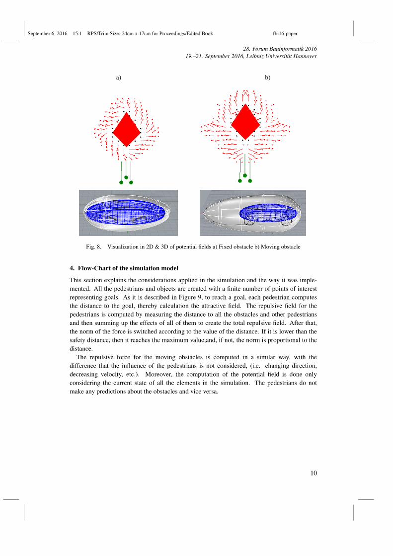
• The range of the potential field is larger in the movement directions of the obstacle, SeeFigure 8b.

• The rotation field is always pointing in the opposite relative direction to the movement ofthe obstacle. Moreover it is positioned in the obstacle center (see Figure 8b).

s = V ∗ F (18)

where:

V = Vector of the velocity

F = Potential field created by the obstacle

If s > 0 then the potential field created by the obstacle is increased by 50 percent.

r = V ∗ R (19)

where:

R=Rotational field created by the obstacle

If r > 0 then the rotational field is inverted

R = −R (20)

The sum of these two effects will help pedestrians avoid the moving obstacles by creatingpaths in the opposite direction of the movement of the obstacles, which leads to safer pathsacross the simulated environment. Figure 8 visualizes the difference between fixed and movingobstacles.

9



a) b)

Fig. 8. Visualization in 2D & 3D of potential fields a) Fixed obstacle b) Moving obstacle

4. Flow-Chart of the simulation model

This section explains the considerations applied in the simulation and the way it was imple-mented. All the pedestrians and objects are created with a finite number of points of interestrepresenting goals. As it is described in Figure 9, to reach a goal, each pedestrian computesthe distance to the goal, thereby calculation the attractive field. The repulsive field for thepedestrians is computed by measuring the distance to all the obstacles and other pedestriansand then summing up the effects of all of them to create the total repulsive field. After that,the norm of the force is switched according to the value of the distance. If it is lower than thesafety distance, then it reaches the maximum value,and, if not, the norm is proportional to thedistance.

The repulsive force for the moving obstacles is computed in a similar way, with thedifference that the influence of the pedestrians is not considered, (i.e. changing direction,decreasing velocity, etc.). Moreover, the computation of the potential field is done onlyconsidering the current state of all the elements in the simulation. The pedestrians do notmake any predictions about the obstacles and vice versa.

10



Fig. 9. Flow Diagram of Potential Fields

Conclusion

In this paper, we present an algorithm allowing pedestrians to avoid obstacles in a dynamicenvironment. Our approach for avoiding obstacles is successful representing the movement ofpedestrians in a dynamic environment. The working stations of the workers and the routes ofthe machines were used as input to set up the environment and simulate the interaction betweenthem. This was done bearing in mind that the pedestrians will avoid both other pedestrians andobstacles. Regarding the machines, or moving obstacles, they will only avoid other obstacles,but the presence of pedestrians does not have an effect on their trajectories.

The developed application outputs the history of the points that describe the trajectory. Thiscan be visualized and may be used to define both the safe routes in a construction site where theworkers can move with low risk, and the high risk areas that the pedestrians should avoid. Thealgorithm used in this project is not limited to simulation of construction sites. Its applicationscan be extended and used to create any scenario where the user wants to find safe paths or zonesfor pedestrians in dynamic environments. An aspect that must to be considered for future workis the pedestrians’ effect on the moving obstacles. Most of the time the machine is not awareof the pedestrians and will not try to avoid them. However, there may be situations where thedriver of the machine sees the pedestrians and may try to avoid them.

11



ReferencesBiedermann, D. H., Kielar, P. M., Handel, O., Borrmann, A. (2014). Towards TransiTUM: A generic

framework for multiscale coupling of pedestrian simulation models based on transition zones. Trans-portation Research Procedia, 495–500.

Biedermann, D. H., Torchiani, C., Kielar, P. M., Willems, D., Handel, O., Ruzika, S., Borrmann, A.(2016). A hybrid and multiscale approach to model and simulate mobility in the context of publicevent. Proc. of the mobil.TUM conference 2016.

Blue, V. J. & Adler, L. (1998). Emergent Fundamental Pedestrian Flows From Cellular Automata.Transportation Research Record, 1644, 29–36.

Colombo, R. M. & Rosini, M. D. (2005). Pedestrian flows and non-classical shocks. MathematicalMethods in the Applied Sciences, 28(13), 1553–1567.

Helbing, D. & Molnár, P. (1995). Social force model for pedestrian dynamics. Physical Review E, 51(5).

Hoogendorn, S. P. & Bovy, P. H. L. (2004). Pedestrian route-choice and activity scheduling theory andmodels, Transportation Research Part B: Methodological, 38(2), 169–190.

Huang, H. C. & Chung, S. Y. (2004). Dynamic visibility graph for path planning. Intelligent Robots andSystems, 3, 2813–2818.

Ijaz, K., Sohail, S., Hashish, S. (2015). A survey of latest approaches for crowd simulation and modelingusing hybrid techniques. 17th UKSIM-AMSS International Conference on Modelling and Simulation,111–116.

Kadry, S., Abdallah, A., Chibli, J. (2012). On The Optimization of Dijkstra’s Algorithm. Informatics inControl, Automation and Robotics, 133, 393–397.

Kielar, P. M. & Borrmann, A. (2016). Modeling pedestrians’ interest in locations: A concept to improvesimulations of pedestrian destination choice, Simulation Modeling Practice and Theory, 47–62.

Kielar, P. M., Biedermann, D. H., Kneidl, A. & Borrmann, A. (2016). A Unified Pedestrian RoutingModel Combining Multiple Graph-Based Navigation Methods, Proceedings of the 11th Conferenceon Traffic and Granular Flow.

Koren, Y. & Borenstein, J. (1991). Potential field methods and their inherent limitations for mobile robotnavigation. Proceedings of the IEEE Conference on Robotics and Automation, 1398–1404.

Lighthill, M. J. & Whitham, G. B. (1955). On kinematic waves. II. A theory of traffic flow onlong crowded roads. Proceedings of the Royal Society of London A: Mathematical, Physical andEngineering Sciences, 229(1178), 317–345.

Richards, P. I. (1956). Shock waves on the highway. Operations research, 4(1), 42–51.

Yufka, A. & Parlaktuna, O. (2009). Performance Comparison of BUG Algorithms for mobile Robots. 5thInternational Advanced Technologies Symposium.

12

construction site pedestrian simulation with moving obstacles

Documents