University of South FloridaScholar Commons

Graduate Theses and Dissertations Graduate School

November 2017

Constructing a Clinical Research DataManagement SystemMichael C. QuinteroUniversity of South Florida, michaelq.quintero@gmail.com

Follow this and additional works at: http://scholarcommons.usf.edu/etd

Part of the Databases and Information Systems Commons

This Thesis is brought to you for free and open access by the Graduate School at Scholar Commons. It has been accepted for inclusion in GraduateTheses and Dissertations by an authorized administrator of Scholar Commons. For more information, please contact scholarcommons@usf.edu.

Scholar Commons CitationQuintero, Michael C., "Constructing a Clinical Research Data Management System" (2017). Graduate Theses and Dissertations.http://scholarcommons.usf.edu/etd/7081

Constructing a Clinical Research Data Management System

by

Michael C. Quintero

A thesis submitted in partial fulfillment of the requirements for the degree of

Master of Science in Computer Science Department of Computer Science and Engineering

College of Engineering University of South Florida

Major Professor: Jared Ligatti, Ph.D. Hao Zheng, Ph.D. Yicheng Tu, Ph.D.

Date of Approval: October 20, 2017

Keywords: Sparse Data Storage, Entity Attribute Value Data Model, Database Modeling, Wide Tables, Clinical Study Data

Copyright © 2017, Michael C. Quintero

i

TABLE OF CONTENTS LIST OF TABLES iii LIST OF FIGURES iv ABSTRACT v CHAPTER 1: INTRODUCTION, BACKGROUND AND MOTIVATION 1

1.1 Introduction and Background 1 1.2 Motivation 2

CHAPTER 2: RELATED WORK 4

2.1 Chapter Summary 4 2.2 Data Storage 4

2.2.1 Wide Table Approach 4 2.2.2 Entity Attribute Value (EAV) Data Model 6 2.2.3 MongoDB and Document Databases 8

2.3 Similar Applications 10 CHAPTER 3: SYSTEM ARCHITECTURE 12

3.1 System Architecture 12 3.2 Authorization and Authentication Architecture 13

CHAPTER 4: IMPLEMENTATION 16

4.1 Chapter Summary 16 4.2 Server Side Application Code 16 4.3 Data Model 17 4.4 User Interface (View) 18 4.5 Memory Caching 19

CHAPTER 5: EVALUATION 22

5.1 Chapter Summary 22 5.2 Test Dataset 22 5.3 Experiments and Experimental Design 23

5.3.1 Reading Entities in EAV 24 5.3.2 Reading Entities in a Wide Table 25 5.3.3 Testing the Cache 26 5.3.4 System Architecture for Experiments 27

5.4 Results 27 5.4.1 Comparing EAV with a Wide Table Results 27 5.4.2 Cache Results 29

5.5 Experimental Results Tables and Figures 30

ii

CHAPTER 6: CONCLUSION 36 REFERENCES 39

iii

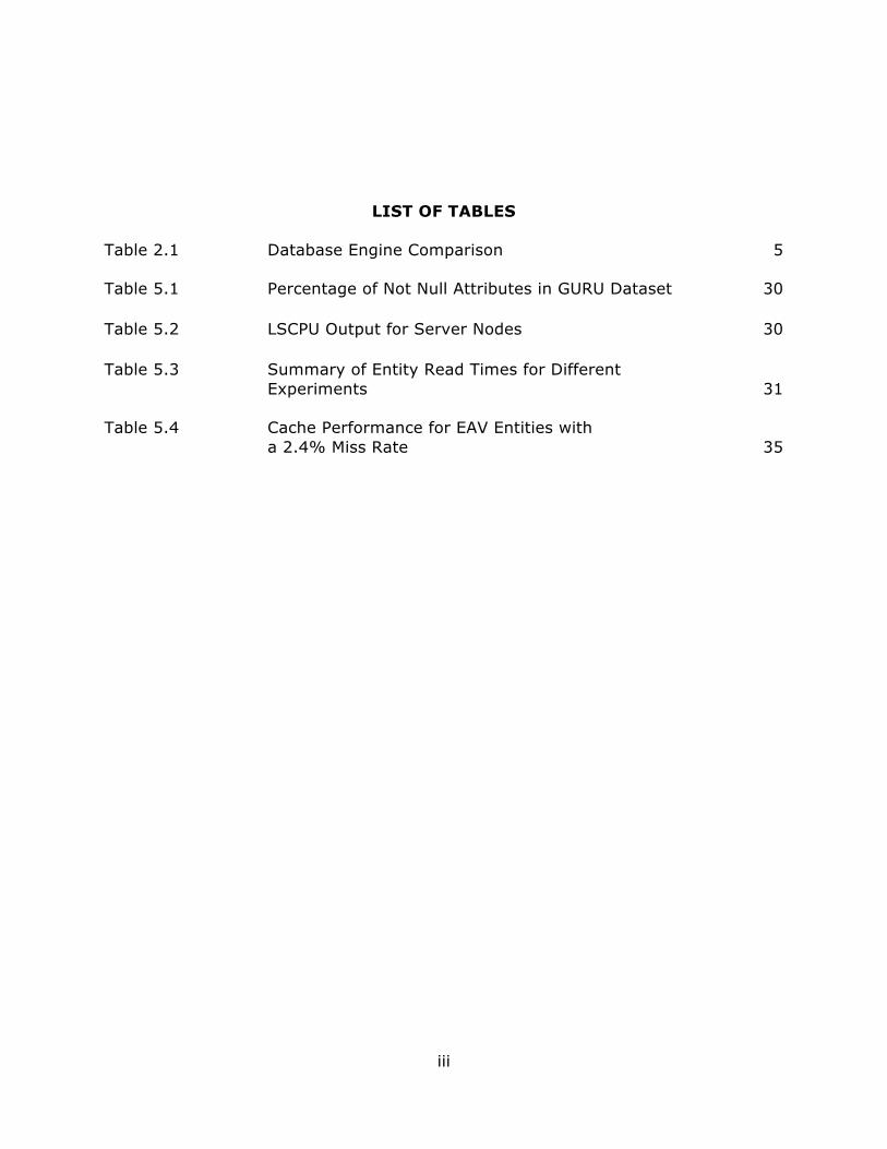
LIST OF TABLES Table 2.1 Database Engine Comparison 5 Table 5.1 Percentage of Not Null Attributes in GURU Dataset 30 Table 5.2 LSCPU Output for Server Nodes 30 Table 5.3 Summary of Entity Read Times for Different Experiments 31 Table 5.4 Cache Performance for EAV Entities with

a 2.4% Miss Rate 35

iv

LIST OF FIGURES Figure 1.1 Overview of GURU Clinical Data Utility 3 Figure 2.1 A Generic EAV Database Schema 11 Figure 3.1 System Architecture 14 Figure 3.2 Authorization Middleware Architecture 15 Figure 4.1 Relational Tables with Automatically Generated Admin Forms 20 Figure 4.2 User Interface of an EAV Entity Attribute Editor 21 Figure 4.3 The Effects of Memcached on Usable Server Cache Space 21 Figure 5.1 Reading an EAV Entity Collection in SQL 31 Figure 5.2 Converting the Results of an EAV Query Into JSON 32 Figure 5.3 EAV Random Entity Read Time 32 Figure 5.4 EAV Bulk (Sequential) Entity Read Time 33 Figure 5.5 Wide Table Random Entity Read Time 33 Figure 5.6 Wide Table Bulk (Sequential) Entity Read Time 34 Figure 5.7 Random Read Performance of EAV Compared with a Wide Table 34 Figure 5.8 Cache Effective Access Time vs Database Entity Read

Time 35

v

ABSTRACT Clinical study data is usually collected without knowing what kind of data is

going to be collected in advance. In addition, all of the possible data points that can

apply to a patient in any given clinical study is almost always a superset of the data

points that are actually recorded for a given patient. As a result of this, clinical data

resembles a set of sparse data with an evolving data schema. To help researchers

at the Moffitt Cancer Center better manage clinical data, a tool was developed

called GURU that uses the Entity Attribute Value model to handle sparse data and

allow users to manage a database entity’s attributes without any changes to the

database table definition. The Entity Attribute Value model’s read performance gets

faster as the data gets sparser but it was observed to perform many times worse

than a wide table if the attribute count is not sufficiently large. Ultimately, the

design trades read performance for flexibility in the data schema.

1

CHAPTER 1: INTRODUCTION, BACKGROUND AND MOTIVATION

1.1 Introduction and Background

The purpose of this thesis is to describe and improve upon the

implementation of a Clinical Data Study Management System Moffitt called the

Genito-Urinary Research Utility (GURU). A Clinical Data Study Management System

(CDSMS) is a class of software that support centralized management of data

generated during the conduct of clinical studies [3]. Of particular interest to the

application was providing an efficient and maintainable mechanism for storing

sparse data in a way that allows the user to be able to make frequent updates to

the data schema with minimal developer intervention and without having to update

the definition of the database tables themselves.

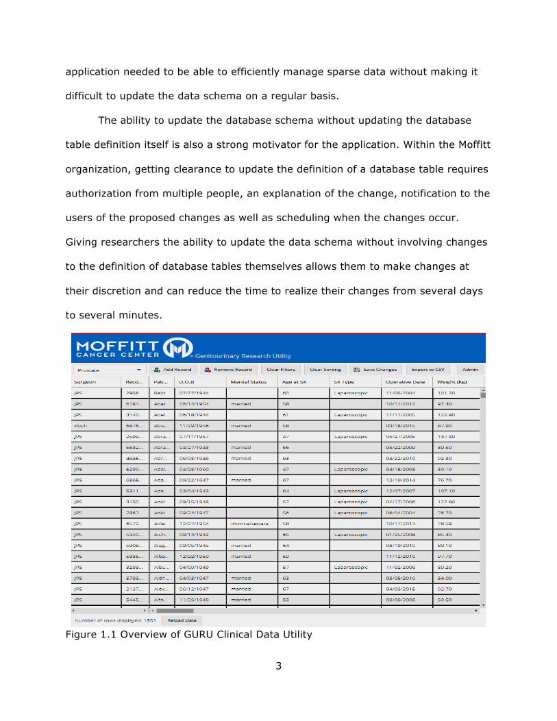
A general overview of the GURU application developed can be seen in Figure

1.1. The user interface is similar to the Microsoft Excel spreadsheet

application: the data is displayed as a grid of values that the user can edit. The

user can also click on a column name to do equality and range filters as well as sort

by column type. On the top bar are buttons for adding and deleting rows, exporting

the dataset to a “.csv” file, removing filters and sorters and a window to an

administrative interface that allows an administrator to manage the data schema

and user roles. Lastly, there is an authorization system in place to allow access to

data depending on user type. There are three types of users: the first can only read

the clinical dataset, the second can only do reads or writes to the dataset and the

last type is an administrator that can read or write to every table in the database,

2

including those that aren’t related to the clinical dataset. Administrators can add

and edit entity attributes as well and can manage user permissions.

1.2 Motivation

The main goal of this project was to create a clinical data study management

system for the Moffitt Cancer Center. The application needs to address our specific

data needs (a sparse dataset that evolves over time) and also meet security

requirements for storing patient health information.

One major motivating factor to develop the application is that GURU is used

to store patient health information and there are strict security requirements for

this data under the The Health Insurance Portability and Accountability Act of 1996

(HIPAA) [9]. Moffitt determines if an application is secure by performing a kind of

security audit on the application for testing the security risk of applications called a

Service Organization Controls 2 Type 2 Report [1]. Applications exist that could be

used to manage a dataset like ours but they were considered a security risk by this

audit, thus making a custom-built application for managing this data a desirable

option.

The nature of our data was also a motivator for the development of the

application. Our dataset can be thought of as a sparse matrix of data that evolves

over time. A sparse dataset is one which has thousands of attributes and for each

of these attributes the value for any given row is typically null [8]. In clinical data

repositories, the number of clinical attributes that can apply to a patient across all

the specialties of medicine can be quite large but only a small number of attributes

have values [17]. We define an evolving dataset as one that has entity attributes

added, updated or removed regularly. To give flexibility to the researchers, our

3

application needed to be able to efficiently manage sparse data without making it

difficult to update the data schema on a regular basis.

The ability to update the database schema without updating the database

table definition itself is also a strong motivator for the application. Within the Moffitt

organization, getting clearance to update the definition of a database table requires

authorization from multiple people, an explanation of the change, notification to the

users of the proposed changes as well as scheduling when the changes occur.

Giving researchers the ability to update the data schema without involving changes

to the definition of database tables themselves allows them to make changes at

their discretion and can reduce the time to realize their changes from several days

to several minutes.

Figure 1.1 Overview of GURU Clinical Data Utility

4

CHAPTER 2: RELATED WORK

2.1 Chapter Summary

This chapter provides a detailed background on the related work surrounding

clinical research data entry web applications. We examine data storage methods as

well as other applications similar to ours.

2.2 Data Storage

As mentioned in the motivation section of Chapter One, the dataset we are

building a Clinical Study Data Management System for is a large amount of sparse

data that has an evolving set of attributes. There has been much research in how

to store this kind of data. We focused our research on three data storage methods:

storing the data in a wide table, the Entity Attribute Value (EAV) database model

and document databases such as MongoDB.

2.2.1 Wide Table Approach

A wide table approach is a straightforward approach to storing a matrix of

sparse data in a standard SQL database. In this approach, we store a row for each

entity and every possible attribute for an entity is stored as a column in the

database. A wide table approach is desirable from a maintainability perspective [8]

but depending on the implementation of the database engine this may not be

practical. Research has shown that a wide table approach for sparse data can be

practically implemented for a sparse dataset provided that the database engine

efficiently stores null values and takes null values into consideration in its indexing

algorithm [8]. Despite this, we found that in the three most popular SQL database

5

engines that a wide table has serious shortcomings when there is a very large

number of columns and frequent column and data updates.

To find out more about the practicality of a wide table approach we

researched the specifications of the three most popular relational database engines:

Oracle, Microsoft SQL Server and MySQL [10]. We examined maximum column

length and indexing performance on sparse columns and found practical limitations

on how effective this can be.

The biggest hurdle to the wide table method for storing sparse data is

column limits. As can be seen in Table 2.1, the maximum column size for standard

tables is around 1,000. Oracle and Microsoft SQL Server do have the option to

create a wide table but its limit is still 30,000 columns. However, the wide table

mode has performance penalties and is intended only for sparse data. In Microsoft

SQL Server, the maximum number of computed columns in a wide table remains

1,024 and the max row size remains about 8,060 bytes [18]. Oracle has similar

limits on row length: the maximum cumulative length of a row’s fixed length

columns is about 32kb despite the max column limit (however, varying length

columns can be about four gigabytes in size) [19].

Table 2.1 Database Engine Comparison [11,12,13 ,19]

In addition, wide tables increase the amount of time it takes to build indexes

and any changes to the database table definitions makes it necessary to recompile

any compiled query plans that exist [14]. Because of this, wide tables suffer a huge

Database Engine Max # Columns Max Row Size Oracle SQL Server (11.1)

1,000 32,768 bytes (fixed length columns)

Microsoft SQL Server (2016)

1,024 8,060 bytes

MySQL (14.8 InnoDB) 1017 65,535 bytes

6

performance penalty for frequent updates to the data or data schema. Microsoft

recommends that wide tables be used for data that is known to be sparse, to

minimize data schema changes and to limit changes to the table data [14]. The

GURU application’s dataset requires frequent changes to the data and schema so

the wide table option was not used.

2.2.2 Entity Attribute Value (EAV) Data Model

The Entity Attribute Value model relies on four major concepts of database

theories: entities, attributes, values and collections. It is efficient for storing sparse

data and supports frequent changes to the data model but it has some

characteristics that make its use difficult in practice.

In databases, an entity is an object that is distinguishable from other objects.

An entity is described using its attributes. A real-world example of an entity would

be a patient at a hospital or an item on sale at a store. In order to be able to

distinguish entities from other entities one often sets a unique identifier (primary

key) to the entity.

A collection is a set of entities. If a hospital is storing patient records, then a

collection would be a set of patient records. One could have a collection for sub

regions of the hospital such as the neurology clinic, the cardiology clinic etc.

Entities are described using their attributes and associated values. An entity

can have many possible attributes that describe it and each of these attributes

possibly has a value describing the attribute. Using our patient example, a patient

would have attributes such as a name and age. A value would be the patient’s

actual name (e.g. “Donald Duck”) [2].

7

Typically, a collection is stored as a SQL table with each row being an entity

and each column being an attribute. The Entity Attribute Value model stores

entities, attributes, values and collections in separate tables. EAV is a generalization

of row modeling [3, 17]. According to Nadkarni, a major researcher in EAV, the

data model is preferable over a wide table approach when many datatypes need to

be represented, some collections are sparse while others are dense and many

possible attributes exist for a collection and the number of attributes is usually

large and fluctuating but the number of values which exist for a given entity is not .

Figure 2.1 shows a simple example of a generic EAV database schema.

Collections, entities, attributes and values all have names and ids. Entities store a

foreign key to the collection they belong to. For each possible attribute, EAV

systems often store a bit of metadata that contains information about the attribute

such as its datatype, validation parameters and sort order. EAV databases often

have a code framework that is driven by this metadata to perform procedures such

as data extraction and UI generation. [3, 17] The values table stores the value and

references the entity it belongs to and the attribute type it is.

The exact implementation of an EAV database schema varies. Other EAV

implementations exist that store different value types in different tables [16]. This

saves space but requires extra join operations to create an entity from the tables.

Storing data using EAV has some obvious benefits. Attributes are stored in

rows, not columns and this makes it possible to update entity attributes without

having to update the data schema. In addition, the sparseness of data has little

impact on the performance of EAV in terms of data extraction and updates since

one only needs to store values they have data for in the values tables and value

8

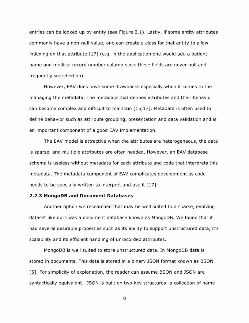
entries can be looked up by entity (see Figure 2.1). Lastly, if some entity attributes

commonly have a non-null value, one can create a class for that entity to allow

indexing on that attribute [17] (e.g. in the application one would add a patient

name and medical record number column since these fields are never null and

frequently searched on).

However, EAV does have some drawbacks especially when it comes to the

managing the metadata. The metadata that defines attributes and their behavior

can become complex and difficult to maintain [15,17]. Metadata is often used to

define behavior such as attribute grouping, presentation and data validation and is

an important component of a good EAV implementation.

The EAV model is attractive when the attributes are heterogeneous, the data

is sparse, and multiple attributes are often needed. However, an EAV database

schema is useless without metadata for each attribute and code that interprets this

metadata. The metadata component of EAV complicates development as code

needs to be specially written to interpret and use it [17].

2.2.3 MongoDB and Document Databases

Another option we researched that may be well suited to a sparse, evolving

dataset like ours was a document database known as MongoDB. We found that it

had several desirable properties such as its ability to support unstructured data, it’s

scalability and its efficient handling of unrecorded attributes.

MongoDB is well suited to store unstructured data. In MongoDB data is

stored in documents. This data is stored in a binary JSON format known as BSON

[5]. For simplicity of explanation, the reader can assume BSON and JSON are

syntactically equivalent. JSON is built on two key structures: a collection of name

9

value pairs called objects and an ordered list of values --i.e. an array [6]. Objects

and lists can be recursively placed inside each other. In MongoDB, an entity is

written as if it were a JSON object and the key value pairs within the object are the

entities attributes. Two major advantages of using this format is that entity

attributes with no value do not need to be recorded so it efficiently stores sparse

data and the entity can be made schemaless and allow arbitrary attributes. There

are not necessarily any restrictions into the type of data inserted into a collection;

however, one can still define a schema if they feel it is necessary. A purely

schema-less design forces the programmer to write defensive code to check data as

it comes out of the database [4].

Documents typically contain only the necessary data with it, making the data

more localized and reducing the need for joins [5]. To understand why, consider the

data necessary to store a blog post in a simple blog application. In MongoDB one

would typically store the title, content and lists of comments, likes or tags for the

blog post in the same document as a series of attribute value pairs. In a relational

database, one would typically have a separate table for likes, comments, blog post

content etc... and join them to get the finished blog post. Because the document

data promotes more locality in the database it makes it better suited to distributed

architectures. A blog post would have all the data needed in the same document

(and therefore the same machine) so a request for it would typically take about one

I/O whereas the relational equivalent may have the data spread across tables,

needing more I/O [5].

Lastly, MongoDB has a few more interesting benefits. It allows the ability to

index on attributes like relational databases and offers speedy access to big data

10

[20]. It is horizontally scalable, meaning one can distribute the database across

multiple nodes when the dataset is large [5].

2.3 Similar Applications

We decided to implement our application using EAV and studied other

applications that used this data model. One of the applications we studied was

TrialDB.

TrialDB is an open source Clinical Study Data Management Tool that runs on

the EAV model. The creators of TrialDB summarized their experience using EAV for

a Clinical Study Data Management System in a paper called “Metadata-driven

creation of data marts from an EAV-modeled clinical research database"[3]. From

TrialDB one can learn how EAV is used to model clinical study data as well as a

method for exporting data from EAV into a conventional format using hash tables

(dictionaries).

The main difference between GURU’s EAV implementation and TrialDB’s is

that TrialDB stores each value type in its own separate table [3]. GURU stores

frequently used types such as strings, floats and integers in the same table and a

foreign key to another table if the data is not one of these. Storing multiple value

types in the same table takes extra space but reduces the number of SQL joins to

read and write entity values the majority of the time.

TrialDB and other applications such as Oracle ClinTrial have robust editors for

handling attribute updates than our application [3,17]. The EAV package we had did

not come with a usable attribute editor out of the box. Rather, it provides users

with forms to edit the physical SQL tables used to generate EAV [16]. To users of

an application, the database is logically a series of rows and columns and the

11

attribute editor should do the logical to physical translation for them [17]. We

discuss steps we took to address attribute updates in Chapter 4.

Figure 2.1 A Generic EAV Database Schema [15]

12

CHAPTER 3: SYSTEM ARCHITECTURE

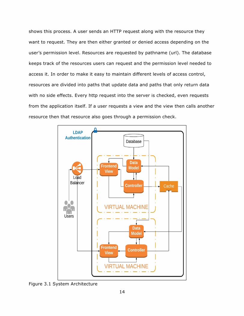
3.1 System Architecture

In this chapter, we will highlight the main features of the GURU system’s

architecture and explain why we made these decisions. The GURU clinical study

data management system architecture looks much like a standard web application.

Figure 3.1 shows the system architecture. One or more virtual machines serve up

instances of the application to the user. The application itself follows a Model View

Controller (MVC) design pattern. The data is stored in an external database server

and the servers share their caches for faster data retrieval. The application is

accessible after authenticating with a type of server called LDAP. Middleware checks

user permissions against application resources. A load balancer divides up user

requests between the virtual machines so different machines can service users in

parallel.

We designed our application to be horizontally scalable. A load balancer is

used to partition the load across multiple servers. New nodes can be added on

demand as needed. In addition to this, the server nodes share their extra cache

memory with other nodes. This allows the application to make use of unused cache

resources. How we were able to pool the caches together will be discussed in

Chapter Four. Caching is necessary because of the distance the data has to travel

from the database. The distance the database is from the servers can change as

the database moves and is usually greater than a few miles while the virtual

13

machines that act as server nodes are hosted in the same room, within a few feet

of each other.

The application software itself is structured according to the Model View

Controller (MVC) design paradigm. What this means is that the application is

separated into three different logical components. The view manages the display of

the data and user inputs. The model manages the data and notifies the view and

controller of any updates. The controller manages the application logic and

responds to input from the user. Using a Model View Controller design pattern is

helpful for achieving partition independent web resources, which aids horizontal

scalability. We would like to note that although we logically designed the application

in an MVC design pattern, web applications are naturally partitioned into a client-

server relationship themselves, making it necessary to put the model, view and

controller on both the client and the server [24].

3.2 Authorization and Authentication Architecture

The application requires strong authentication and authorization mechanisms

to host patient health information. An overview of these mechanisms can be seen in

Figure 3.2. Authentication was done using an LDAP server. LDAP is an open,

efficient, extensible, and popular means of interacting with the data contained in

directory servers that has strong support for authentication mechanisms like

password encryption and is commonly used to store user data [25]. Moffitt uses

one LDAP system for all its web applications so that users only need to remember

one username and password and authentication can be managed in one place.

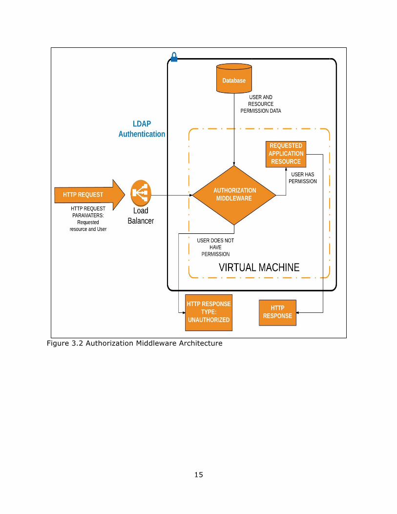
Authorization is done via application server middleware that runs on every

request to the server before the application itself processes the data. Figure 3.2

14

shows this process. A user sends an HTTP request along with the resource they

want to request. They are then either granted or denied access depending on the

user’s permission level. Resources are requested by pathname (url). The database

keeps track of the resources users can request and the permission level needed to

access it. In order to make it easy to maintain different levels of access control,

resources are divided into paths that update data and paths that only return data

with no side effects. Every http request into the server is checked, even requests

from the application itself. If a user requests a view and the view then calls another

resource then that resource also goes through a permission check.

Figure 3.1 System Architecture

15

Figure 3.2 Authorization Middleware Architecture

16

CHAPTER 4: IMPLEMENTATION

4.1 Chapter Summary

In this chapter, we discuss our implementation of the GURU web application.

We divide up our discussion into four parts: Server side application code, the data

model, the user interface and memory caching.

4.2 Server Side Application Code

The application server code is written using the Django Web Framework.

Django is a python web framework that is made to facilitate fast development and

pragmatic design [27]. Django is competitor to other popular web frameworks such

as ASP.NET, Flask and Ruby on Rails and has very similar functionality. One of the

main reasons Django is used is due to their claims of having strong security

protection against many common web application vulnerabilities [28]. Evaluating

these claims is beyond the scope of this paper. We used Django to serve up files,

handle authentication, authorization and work with the database.

We relied on Django’s pre-built user account system and administrative

interface for our application. The user account system facilitates the authentication

of users into the database and the administrative interface provides admins with

the ability to manage the user accounts system as well as any table in the

database. The user account system also has built in support for defining user

groups. These user groups are used by the middleware discussed in Chapter Three

to provide access control to the user based on their role.

17

Django has a class based system that we used to provide web services. The

web services are accessed by url, usually via a POST or a GET method. Apart from

the pre-built Django web services that handle authentication and admin

functionalities, there is a web service to provide the user interface to the user and a

web service that the user interface uses to read and write to the database. The web

service that works with the data set does the logical conversion of EAV data into

row-column format upon read operations and provide data validation and error

checking on write operations.

4.3 Data Model

The data is built using Django’s Object Relational mapper (ORM). An object

relational mapper is a library that automates the transfer of data stored in a

relational database into the kind of class objects found in application code. It allows

developers to define class objects that represent database tables in a relational

database and use these class objects to perform basic database operations such as

create, update, read and delete operations in python with method calls instead of

raw SQL statements. This can greatly speed up development. [26]. In addition to

the basic CRUD operations, the Django ORM provides some security measures like

automatic type checking, and allows the developer to define validators and display

functions. The display functions are used to format data, e.g. displaying a floating-

point number in a percentage format.

The downside of using the Django Object Relational mapper is that when

reading data, the auto-generated SQL statements made by Django can have a

significant performance penalty if it creates too many objects from the data. Its

18

impact made it more efficient to use native SQL statements than to rely on the

Django ORM for reading EAV entities.

Our data model made heavy use of other libraries written with Django’s ORM.

We used the default Django package that sets up the database tables necessary for

basic security features like authorization and authentication. In addition to that, we

used the EAV data model discussed in Chapter Two for our system. An EAV library

called Django-EAV [16] was used to accomplish this.

4.4 User Interface (View)

The main user interface of the application can be seen in Figure 1.1. The user

interface takes data that has been logically converted from an EAV format to a row,

column format for the user to browse through the data. The user has the ability to

sort and filter data based on his needs. In addition, the user can also add and

remove entity records and edit attributes for existing records. On the top left of

Figure 1.1, in the field marked “Prostate”, users can click on this to select a

different cancer type to view. The data is organized based on the kind of cancer.

The data is presented to the user as if it were in row-column format, but internally

uses the EAV data model. As it relates to EAV, a cancer type is a collection, a row is

an entity, and an attribute is a column.

Django also provides an administrative user interface that automatically

creates forms for managing all the relational database tables. Figure 4.1 shows the

homepage of this administrative view. Clicking on any of the tables leads to a form

where the user can create, update and delete records in the table.

As discussed in Chapter 2, the relationships between the EAV tables and the

metadata are complex so to manage that part of the database we found it easier to

19

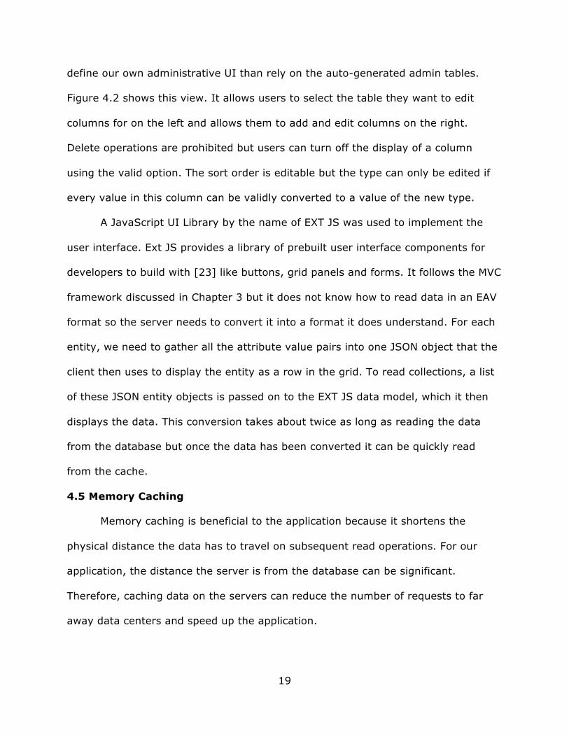
define our own administrative UI than rely on the auto-generated admin tables.

Figure 4.2 shows this view. It allows users to select the table they want to edit

columns for on the left and allows them to add and edit columns on the right.

Delete operations are prohibited but users can turn off the display of a column

using the valid option. The sort order is editable but the type can only be edited if

every value in this column can be validly converted to a value of the new type.

A JavaScript UI Library by the name of EXT JS was used to implement the

user interface. Ext JS provides a library of prebuilt user interface components for

developers to build with [23] like buttons, grid panels and forms. It follows the MVC

framework discussed in Chapter 3 but it does not know how to read data in an EAV

format so the server needs to convert it into a format it does understand. For each

entity, we need to gather all the attribute value pairs into one JSON object that the

client then uses to display the entity as a row in the grid. To read collections, a list

of these JSON entity objects is passed on to the EXT JS data model, which it then

displays the data. This conversion takes about twice as long as reading the data

from the database but once the data has been converted it can be quickly read

from the cache.

4.5 Memory Caching

Memory caching is beneficial to the application because it shortens the

physical distance the data has to travel on subsequent read operations. For our

application, the distance the server is from the database can be significant.

Therefore, caching data on the servers can reduce the number of requests to far

away data centers and speed up the application.

20

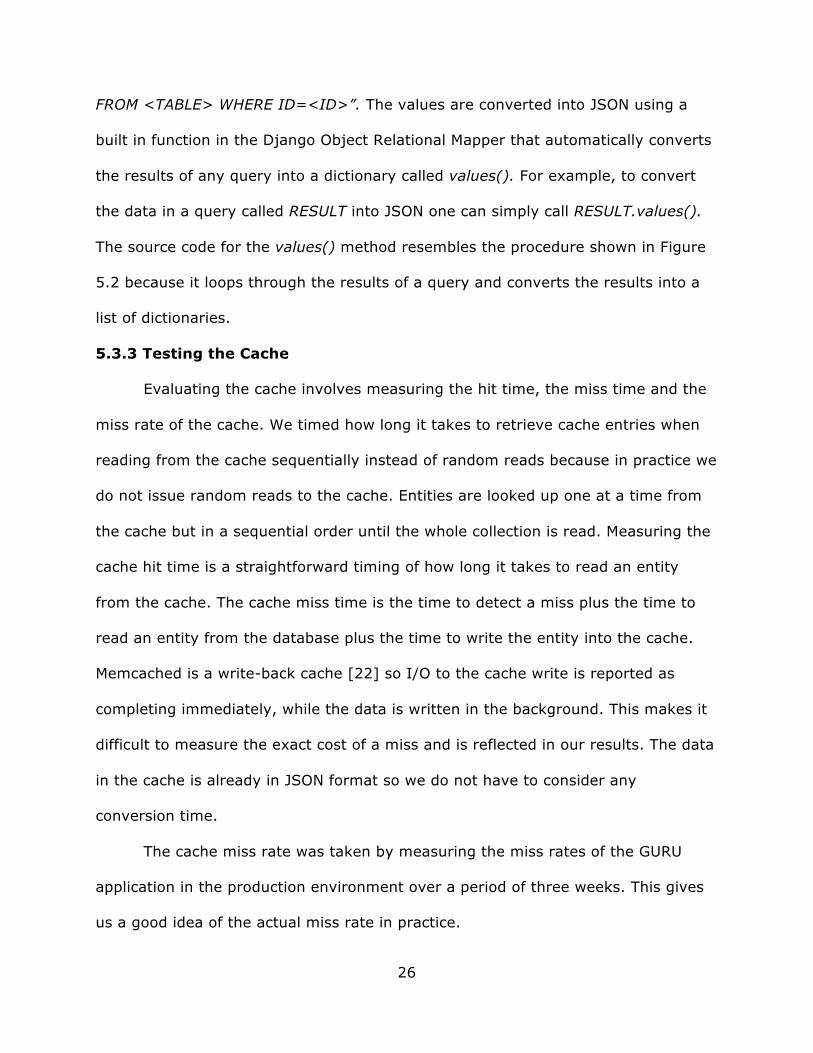
To implement our memory caching system, we used a technology called

Memcached. The main benefit of memcached is that it facilitates the sharing of

usable cache space across different server nodes, increasing the usable cache

space. Figure 4.3, which is from the Memcached organization [21], illustrates the

effect memcached has on servers. When used, two or more servers can share their

cache spaces and increase the amount of cache each server has to work with.

Memcached uses a client-server architecture to store key value pairs in

memory. It has a server which holds a hash table consisting of the key value pairs

and clients (application servers) make reads and writes to the server. The server

manages when to evict or reuse object memory but the client can make requests

for when to invalidate an item in the cache [22]. We evaluate the cache

performance in the next chapter.

Figure 4.1 Relational Tables with Automatically Generated Admin Forms

21

Figure 4.2 User Interface of an EAV Entity Attribute Editor

Figure 4.3 The Effects of Memcached on Usable Server Cache Space [21]

22

CHAPTER 5: EVALUATION

5.1 Chapter Summary

In this chapter, we evaluate various parts of the implementation, primarily

focusing on evaluating the data model’s read performance from the database and

the cache.

5.2 Test Dataset

One of the reasons an EAV database was chosen for the application because

research claims it is effective in storing sparse data. To measure if there was any

potential benefit to this in our application we designed our dataset to show us the

performance of EAV across various levels of sparseness. Five collections were

created with an equal number of attributes and various levels of sparseness. We

measured a table that was empty, 25% full, 50% full, 75% full and completely full

in terms of non-null value count for the entity’s attributes. To make the attributes

for the collection we combined every attribute available to every entity in all

collections in the GURU application. In total, there are 285 attributes in the

collection. This is not an extremely large number of attributes but it is

representative of the attribute count currently in use by the GURU application.

As a control for the EAV dataset, five wide tables with various levels of non-

null attributes were created. The non-null attribute count in the wide tables

matches the EAV dataset: there is a table that is empty, 25% full, 50% full, 75%

full and completely full in terms of non-null value count. There is one column for

23

every attribute in the table and the attributes are identical to the ones measured in

the EAV dataset.

The EAV and control collections were seeded with data so that attribute-value

pairs are randomly dispersed throughout the data. 10,000 entities were inserted

into each collection Then, for each entity a random subset of all the attributes was

selected and random values were inserted for those attributes into that entity. The

size of the random slice is determined by how sparse the dataset will be. For

example, the size of the random subset of attributes for entities in the 50% full

table is 142 because there are 285 attributes and 142 = %&'%

.

To simplify our evaluation, only the count of non-null attribute-value pairs

within an entity is considered. Different datatypes have different sizes and this can

affect the expected read performance for that datatype. However, the possible

impact that this could have on our results is limited by the random dispersion of the

attribute-value pairs across entities and therefore we do not consider the datatypes

of the values we are reading in our analysis. On average, every entity read from a

given collection will be about the same size.

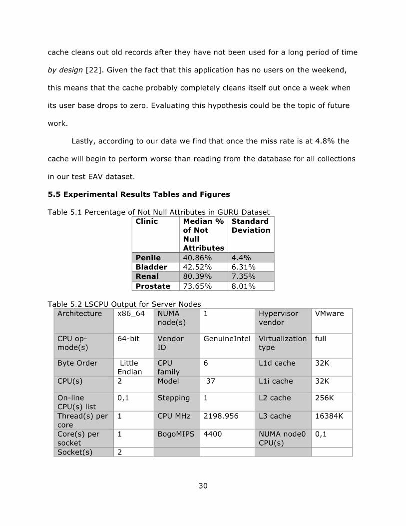
Whether or not the data model is useful to our organization depends on how

well it can handle our actual dataset. Figure 5.1 shows each clinical collection, the

median non-null value percentage and the standard deviation of this measurement.

Each dataset is different but as we can see, the range is about 40-80% full in the

GURU application.

5.3 Experiments and Experimental Design

The experiments mainly revolve around evaluating the performance of our

data model and how efficiently we can retrieve data. We begin by comparing the

24

read performance of EAV against a wide table. Then we evaluate the performance

of the cache.

To perform random reads on a collection, a random entity was selected to be

read from the database 50,000 times. For each collection, a list of all the entity ids

in that collection was retrieved and random ids were selected using pythons pre-

built random number generating library: random. The time chosen is the median of

all 50,000 read times. To perform a bulk read, the entire collection from the

database is read 200 times for each collection. The entity read time is taken to be

the time to read a collection divided by the number of entities in the collection.

Each bulk query is recorded into a list and the median entity read time of all those

read times is taken to represent the amount of time to read an entity in a bulk

query. The standard deviation of the times recorded is also taken for random and

bulk reads.

The time measured is the time from when the request is made until the data

is in JSON format. The JSON format we take as final is a list of dictionaries. Each

dictionary contains all the attribute value pairs for a particular entity.

5.3.1 Reading Entities in EAV

Figure 5.1 demonstrates the reading procedure designed in SQL. The query

returns a list of values consisting of the entity id for that value, the attribute name

and the value. The database schema for the query can be seen in Figure 2.1. The

value and attributes table are joined on the attribute_id. Then, the entity table is

filtered on the collection_id we want to retrieve and this result is joined with the

attribute-value table on the entity ID. Lastly, the values are filtered on their

attribute’s datatype in a CASE WHEN statement and this is returned as the final

25

value for that attribute-value pair. The resulting SET OF VALUES is ordered by the

entity id.

Figure 5.1 demonstrates the procedure to retrieve a bulk collection of

entities. The procedure to retrieve a single entity at a time for random reads is

almost identical except that instead of filtering the entity table on the collection_id ,

filter it on the id of the entity to extract from the database. There is no need to

retrieve the entity id in the final result or order on the entity id like in Figure 5.1.

Since the procedure is almost identical we do not provide a figure that shows how

to retrieve a single entity at a time and this is left as an exercise to the reader.

After this, the result of the query is converted into JSON format for the client

side to be able to read and display the data to the user. The client side reads a list

of JSON objects where the key-value pairs for the object are attribute-value pairs

for the entity. Figure 5.2 demonstrates the JSON conversion procedure for a bulk

retrieval of entities. The entity query is retrieved in the first line and then for each

entity in the query ad dictionary is made and added to the list. The query is ordered

by entity id so one can loop through the query and create a new dictionary for the

next entity when the id changes. The end result is converted into a JSON string and

returned to the client. The procedure to convert a single entity into JSON is almost

identical and is left as an exercise to the reader.

5.3.2 Reading Entities in a Wide Table

The read procedure to read entities from a wide table is straightforward. To

perform a bulk query to a table called <TABLE> the entire collection is read with

the query “SELECT * FROM <TABLE>”. To perform a random entity read to an

entity whose id is <ID>, one entity is read at a time with the query “SELECT *

26

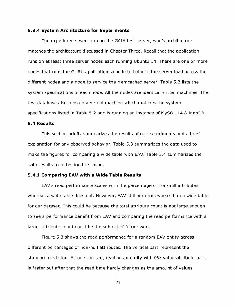
FROM <TABLE> WHERE ID=<ID>”. The values are converted into JSON using a

built in function in the Django Object Relational Mapper that automatically converts

the results of any query into a dictionary called values(). For example, to convert

the data in a query called RESULT into JSON one can simply call RESULT.values().

The source code for the values() method resembles the procedure shown in Figure

5.2 because it loops through the results of a query and converts the results into a

list of dictionaries.

5.3.3 Testing the Cache

Evaluating the cache involves measuring the hit time, the miss time and the

miss rate of the cache. We timed how long it takes to retrieve cache entries when

reading from the cache sequentially instead of random reads because in practice we

do not issue random reads to the cache. Entities are looked up one at a time from

the cache but in a sequential order until the whole collection is read. Measuring the

cache hit time is a straightforward timing of how long it takes to read an entity

from the cache. The cache miss time is the time to detect a miss plus the time to

read an entity from the database plus the time to write the entity into the cache.

Memcached is a write-back cache [22] so I/O to the cache write is reported as

completing immediately, while the data is written in the background. This makes it

difficult to measure the exact cost of a miss and is reflected in our results. The data

in the cache is already in JSON format so we do not have to consider any

conversion time.

The cache miss rate was taken by measuring the miss rates of the GURU

application in the production environment over a period of three weeks. This gives

us a good idea of the actual miss rate in practice.

27

5.3.4 System Architecture for Experiments

The experiments were run on the GAIA test server, who’s architecture

matches the architecture discussed in Chapter Three. Recall that the application

runs on at least three server nodes each running Ubuntu 14. There are one or more

nodes that runs the GURU application, a node to balance the server load across the

different nodes and a node to service the Memcached server. Table 5.2 lists the

system specifications of each node. All the nodes are identical virtual machines. The

test database also runs on a virtual machine which matches the system

specifications listed in Table 5.2 and is running an instance of MySQL 14.8 InnoDB.

5.4 Results

This section briefly summarizes the results of our experiments and a brief

explanation for any observed behavior. Table 5.3 summarizes the data used to

make the figures for comparing a wide table with EAV. Table 5.4 summarizes the

data results from testing the cache.

5.4.1 Comparing EAV with a Wide Table Results

EAV’s read performance scales with the percentage of non-null attributes

whereas a wide table does not. However, EAV still performs worse than a wide table

for our dataset. This could be because the total attribute count is not large enough

to see a performance benefit from EAV and comparing the read performance with a

larger attribute count could be the subject of future work.

Figure 5.3 shows the read performance for a random EAV entity across

different percentages of non-null attributes. The vertical bars represent the

standard deviation. As one can see, reading an entity with 0% value-attribute pairs

is faster but after that the read time hardly changes as the amount of values

28

increases. This is probably because the results of a random read take up one block

of data from the database regardless if the entity is 25% full or 100% full. An

empty entity is read faster because no data is returned from the query. Using EAV

to read a random entity offers almost no performance benefit. However, Figure 5.4

shows the time to read an EAV entity in a bulk query and from this figure we can

see that the performance appears to scale linearly with the percentage of non-null

attributes. Sparser data is read faster. This is probably because the data returned

by a large number of entities takes less blocks of memory if the data is sparse and

therefore less data needs to be returned from the database.

In contrast, the read performance of Wide Tables does not scale linearly with

the amount of non-null attributes and no performance benefit is observed for

sparser data. In fact, we observed the bulk read performance actually may be

getting worse as the data became sparser. Figure 5.5 shows the read performance

of random Wide Table reads to EAV entities. The vertical bars represent the

standard deviation. From the figure, we find that there is no correlation between

the percentage of non-null attribute value pairs and the entity read time for a

random entity. Again, this is probably because reading a random entity takes up

one block to store in a database regardless of its data density. Figure 5.6 shows the

entity read time for a bulk query using a wide table. The dotted trend line shows a

slight downward trend and the trend seems to show that tables that are denser

tend to read slightly faster and that tables with no null values read the fastest of

all. However, we note that the read times differ by only a few microseconds making

it a negligible performance penalty for this dataset. Testing to see if the trend gets

stronger when the number of columns increases could be the topic of future work.

29

The read performance of the wide table far exceeded the read performance

of EAV for our dataset. Figure 5.7 shows the random read performance of the two

compared against each other and it is apparent that the random read performance

is about five times worse when using EAV. This is probably due to the cost of

joining tables. This performance difference is even more pronounced on bulk reads.

As Table 5.3 shows, the bulk read performance is about four orders of magnitude

faster with a wide table (10,000-20,000 times faster). Clearly Wide Tables are

faster on our dataset.

Lastly, the amount of time it takes to read an empty entity is quite expensive

for EAV. From Table 5.3, it takes approximately 1.2 seconds to read a random

empty entity in EAV at random and 50 milliseconds to read an empty EAV entity in

bulk. Compare this with a median time of 2 milliseconds to detect an empty entity

collection if the entities were deleted and we can see that reading an empty entity

can have a significant performance impact. Special care should be taken to delete

entities for which no attribute-value pair exists.

5.4.2 Cache Results

Table 5.4 summarizes the cache hit time, miss time and effective access time

for the EAV dataset. The miss rate observed in the production environment for the

application is 2.4%. The hit time and miss time scales linearly with the amount of

non-null attribute pairs meaning sparser data performs better on the cache. Figure

5.5 shows the effective access time compared with the database read time. We

found that the cache is about 48-54% faster than reading from the database.

The cache speedup was less than expected. It is the writer’s hypothesis that

the speedup is due to a high miss rate in the cache caused by the fact that the

30

cache cleans out old records after they have not been used for a long period of time

by design [22]. Given the fact that this application has no users on the weekend,

this means that the cache probably completely cleans itself out once a week when

its user base drops to zero. Evaluating this hypothesis could be the topic of future

work.

Lastly, according to our data we find that once the miss rate is at 4.8% the

cache will begin to perform worse than reading from the database for all collections

in our test EAV dataset.

5.5 Experimental Results Tables and Figures

Table 5.1 Percentage of Not Null Attributes in GURU Dataset Clinic

Median % of Not Null Attributes

Standard Deviation

Penile 40.86% 4.4% Bladder 42.52% 6.31% Renal 80.39% 7.35% Prostate 73.65% 8.01%

Table 5.2 LSCPU Output for Server Nodes

Architecture x86_64 NUMA node(s)

1 Hypervisor vendor

VMware

CPU op-mode(s)

64-bit Vendor ID

GenuineIntel Virtualization type

full

Byte Order Little Endian

CPU family

6 L1d cache 32K

CPU(s) 2 Model 37 L1i cache 32K

On-line CPU(s) list

0,1 Stepping 1 L2 cache 256K

Thread(s) per core

1 CPU MHz 2198.956 L3 cache 16384K

Core(s) per socket

1 BogoMIPS 4400 NUMA node0 CPU(s)

0,1

Socket(s) 2

31

Table 5.3 Summary of Entity Read Times for Different Experiments Percent of

Non Null

Attributes

Wide Table

Random

Wide Table

Bulk

EAV

Random

EAV Bulk

0% 0.01186502 5.11538E-06 0.853406906 0.051851893

25% 0.012344956 4.94458E-06 1.042161465 0.053742348

50% 0.011809468 3.90811E-06 1.074842811 0.056616105

75% 0.01225543 4.65827E-06 0.913892388 0.057458689

100% 0.01274991 3.22082E-06 1.226836562 0.058835183

SELECT entities.id, attribute.name, ( CASE WHEN datatype='text' THEN value_text WHEN datatype='float' THEN Cast(value_float AS CHAR(64) ) WHEN datatype='date' THEN Cast(value_date AS CHAR(64)) WHEN datatype='int' THEN Cast(value_int AS CHAR(64)) WHEN datatype='fraction' THEN value_text WHEN datatype='percent' THEN Cast(value_text AS CHAR(64)) end) AS value FROM ( SELECT * FROM entities WHERE collection_id = <COLLECTION_ID>) AS entities INNER JOIN SELECT id, attribute_id, entity_id, value_text, value_float, value_int, value_date FROM value) AS values ON entities.id= values.entity_id LEFT JOIN (SELECT id, slug , datatype FROM attribute) AS attributes ON values.attribute_id= attributes.id ORDER by rows.id;

Figure 5.1 Reading an EAV Entity Collection in SQL

32

#BULK READ ENTITIES CALLS THE SQL QUERY ABOVE entity_query = DO_EAV_QUERY(collection_id) entity_list = [] current_entity_dict = {} # initialize to first entity last_entity_id = data[‘id’] # A value looks like : (row_id, slug, value) for entity_id, attribute,value in data: if last_entity_id == entity_id: result[attribute] = value else: current_entity_dict['id'] = row_id entity_list.append(current_entity_list) current_entity_dict = {} last_entity_id = entity_id result[attribute] = value return JSONIFY(entity_list)

Figure 5.2 Converting the Results of an EAV Query Into JSON

Figure 5.3 EAV Random Entity Read Time

33

Figure 5.4 EAV Bulk (Sequential) Entity Read Time

Figure 5.5 Wide Table Random Entity Read Time

34

Figure 5.6 Wide Table Bulk (Sequential) Entity Read Time

Figure 5.7 Random Read Performance of EAV Compared with a Wide Table

35

Figure 5.8 Cache Effective Access Time vs Database Entity Read Time Table 5.4 Cache Performance for EAV Entities with a 2.4% Miss Rate

Percent of Non-Null Attributes

25% 50% 75% 100%

Cache Hit Time

4.47788E-05 0.000411878 0.000103118 0.000927662

Cache Miss Time

1.220474958 1.132763863 1.221189976 1.277502775

Effective Access Time

0.029335103 0.027588326 0.029409203 0.031565465

36

CHAPTER 6: CONCLUSION

The GURU application was created to help researchers manage clinical

studies. Clinical patient data resembles a set of constantly evolving, sparse data so

the data model needs to take this into account. To help researchers manage their

data, Moffitt constructed a web application with an interface to read and write data

in a spreadsheet-like format. To allow the researchers the flexibility to manage their

data schema, an administrative user interface was constructed to allow the user to

manage read, write, update and create entity attributes without having to update

the schema of the underlying SQL tables.

To store sparse, evolving data there were many choices considered such as a

wide table, the Entity Attribute Value Model and MongoDB. The Wide Table

approach was inflexible and hindered by maximum column limits. MongoDb was

promising but there is a lack of expertise to use it within the organization. Given

the options, the Entity Attribute Value model was chosen for the data model since it

has no limits on attribute count and offers the user flexibility to make frequent

updates to their data schema.

When compared with a Wide Table we found that the Entity Attribute Value

(EAV) model performed many times worse in terms of random and sequential read

performance. However, it was observed that the read performance of EAV scales

linearly with the density of the data: sparser data results in faster reads. Wide

Table read performance had no conclusive trend for random reads but it was

observed that as the data grows sparser the read performance gets slightly worse.

37

Given the difference in performance between a wide table and EAV it would be

more efficient to use a wide table to read the data. However, since a Wide Table’s

sequential read performance gets worse as data gets sparser but EAV’s gets better

as data gets sparser it may be the case that read performance of EAV will

eventually get better than a Wide Table if the attribute count is much larger and the

data remains sparse. Exploring this could be the topic of future work.

To improve the read performance of the EAV data model, a distributed

caching system called Memcached was introduced into the application. After an

evaluation, it was observed that the cache halves the effective access time of

entities from the database and the main reason why the cache doesn’t do better

than it already does is due to a high miss rate. Even with caching in place, the

performance is worse than a wide table.

EAV reads worse than a Wide Table for the GURU dataset, but it offers

flexibility that a Wide Table does not. Updating an entity attribute in a Wide Table

involves changing the SQL database schema. Updating an entity attribute in EAV

can be done by writing to the attributes table. Within the Moffitt organization,

changes to a SQL database schema involve changes to the Object Relational

Mapper code, approval from more than one IT professionals in the organization, a

presentation of the proposed changes and when the changes are to occur. This

process can take days. Using an EAV data model allows researchers to update the

data schema at their own discretion and makes it possible for the researchers to

have a constantly evolving dataset.

The GURU application gives clinical researchers at Moffitt the ability to

manage a sparse set of data whose attributes frequently change. It uses the Entity

38

Attribute Value model, which reads slowly but allows users to make changes to an

entity’s data schema without changing the definition of the database table. Caching

slightly improves the performance but it is still worse than a wide table for its

current dataset. Ultimately, the GURU application’s use of EAV sacrifices read

performance for flexibility in the data schema.

39

REFERENCES

[1] "SOC for Service Organizations: Information for Service Organizations." Service Organization Controls (SOC) Reports for Service Organizations - AICPA. American Institute of Certified Public Accountants, 2017. Web. <https://www.aicpa.org/InterestAreas/FRC/AssuranceAdvisoryServices/Pages/ServiceOrganization%27sManagement.aspx>. [2] Ramakrishnan, Raghu, and Johannes Gehrke. "2.2 Introduction to Database Design/Entities, Attributes, and Entity Sets." Database Management Systems. 3rd ed. Vol. 1. New York,NY: McGraw-Hill, 2003. 29-30. Print. [3] Brandt, Cynthia A., Richard Morse, Keri Matthews, Kexin Sun, Aniruddha M. Deshpande, Rohit Gadagkar, Dorothy B. Cohen, Perry L. Miller, and Prakash M. Nadkarni. "Metadata-driven creation of data marts from an EAV-modeled clinical research database." International Journal of Medical Informatics (2002): 1-17 [4] “Collections.” Meteor (2017) 2. Web <https://guide.meteor.com/collections.html#mongo-collections > Introduction to using MongoDB in the context of a web application [5] “MongoDB Architecture.” MongoDB (2016): 2. Web. https://www.MongoDB.com/MongoDB-architecture>. [6] "The JSON Data Interchange Format." ECMA International (2013): 2. Web. <http://www.ecma-international.org/publications/files/ECMA-ST/ECMA-404.pdf>. [7] "Optimizing Data Size." MySQL Reference Manual. MySQL, 2016. Web. 23 July 2017. <https://dev.mysql.com/doc/refman/5.5/en/data-size.html>. MySQL Null values take space [8] Chu, Eric, Jennifer Beckmann, and Jeffrey Naughton. " The case for a wide-table approach to manage sparse relational data sets." SIGMOD '07 Proceedings of the 2007 ACM SIGMOD international conference on Management of data (2017): 821-32. ACM Digital Library. Web. 12 July 2017. <http://dl.acm.org/citation.cfm?id=1247571>. [9] "Summary of the HIPAA Security Rule." Hhs.gov. U.S. Department of Health & Human Services, 26 July 2013. Web. 23 July 2017. <https://www.hhs.gov/hipaa/for-professionals/security/laws-regulations/index.html>.

40

[10] "DB-Engines Ranking." Db-engines.com. DB Engines, 1 July 2017. Web. 22 July 2017. Database engines ranked by popularity <https://db-engines.com/en/ranking>. [11] "Maximum Capacity Specifications for SQL Server." Microsoft SQL Server. Microsoft, 2016. Web. 22 July 2017. <https://docs.microsoft.com/en-us/sql/sql-server/maximum-capacity-specifications-for-sql-server>. Microsoft SQL Server Limitations [12] Logical Database Limits." Oracle Database Reference. Oracle, 2016. Web. 23 July 2017. <https://docs.oracle.com/cd/B28359_01/server.111/b28320/limits003.htm#i288032>. Oracle Database Limits [13] "Limits on InnoDB Tables." MySQL Reference Manual. MySQL, n.d. Web. <https://dev.mysql.com/doc/refman/5.7/en/innodb-restrictions.html>. MySQL Database Limits [14] "Performance Considerations for Wide Tables." technet.microsoft.com Performance Considerations for Wide Tables, n.d. Web. <https://technet.microsoft.com/en-us/library/cc645884(v=sql.105).aspx>. [15] Raszczynski, Robert. "The EAV Data Model." Inviqa.com. Inviqa, 21 Oct. 2010. Web. 25 July 2017. <https://inviqa.com/blog/EAV-data-model>. [16] Gelvin, David, David McCann, Bruno Tavares, and Hamdi Salhoul. Django-EAV. Computer software. GitHub. Mvpdev, 26 Jan. 2017. Web. 27 July 2017. <https://github.com/mvpdev/django-EAV>. [17] Dinu V, Nadkarni P. "Guidelines for the effective use of entity-attribute-value modeling for biomedical databases." International journal of medical informatics;76(11-12):769–79. doi: <10.1016/j.ijmedinf.2006.09.023>. [18] "Special Table Types." Technet.microsoft.com. Microsoft, 2016. Web. 29 July 2017. <https://technet.microsoft.com/en-us/library/ms186986(v=sql.105).aspx>. SQL Server Wide Tables [19] "System Limits." Docs.oracle.com. Oracle, 2015. Web. 30 July 2017. <https://docs.oracle.com/cd/E11882_01/timesten.112/e21643/limit.htm#TTREF455>. [20] Han, Jing, Haihong E, Guan Le, and Jian Du. "Survey on NoSQL database." <http://ieeexplore.ieee.org/. IEEE, 2011>. Web. 2 Aug. 2017. [21] About Memcached.” <Memcached.org, memcached.org/>. Accessed 3 Sept. 2017.

41

[22] Memcached Wiki. Memcached, May 2016, <https://github.com/memcached/memcached/wiki>. Accessed 4 Sept. 2017. [23] “Ext JS Overview.” Sencha Ext JS, Sencha, <www.sencha.com/products/extjs/#overview>. Accessed 5 Sept. 2017. [24] Leff, Avraham, and James T Rayfield. “Web-Application development using the Model/View/Controller design pattern.” Enterprise Distributed Object Computing Conference, 2001. EDOC '01. Proceedings. Fifth IEEE International. IEEE, <http://ieeexplore.ieee.org/document/950428/ >. [25] “Getting Started with LDAP.” LDAP.COM, UnboundID, <www.ldap.com/getting-started-with-ldap>. [26] “Object-Relational mappers (ORMs).” Fullstackpython.com, Full Stack Python, <www.fullstackpython.com/object-relational-mappers-orms.html>. Accessed 12 Sept. 2017. [27] “About Django.” Django Project, Django, <www.djangoproject.com/>. Accessed 15 Sept. 2017. [28] “Security in Django.” Djangoproject.com, Django, Apr. 2017, docs.djangoproject.com/en/1.11/topics/security/. Accessed 16 Sept. 2017.