Constraint-based Optimization and Utility

Elicitation using the Minimax Decision

Criterion

Craig Boutilier a,∗, Relu Patrascu a,1, Pascal Poupart a,2,

Dale Schuurmans c,1

aDepartment of Computer Science, University of Toronto, Toronto, ON, M5S3H5, CANADA

bSchool of Computer Science, University of Waterloo, Waterloo, ON, CANADAcDepartment of Computing Science, University of Alberta, Edmonton, AB, T6G

2E8, CANADA

Abstract

In many situations, a set of hard constraints encodes the feasible configurations ofsome system or product over which multiple users have distinct preferences. How-ever, making suitable decisions requires that the preferences of a specific user fordifferent configurations be articulated or elicited, something generally acknowledgedto be onerous. We address two problems associated with preference elicitation: com-puting a best feasible solution when the user’s utilities are imprecisely specified; anddeveloping useful elicitation procedures that reduce utility uncertainty, with min-imal user interaction, to a point where (approximately) optimal decisions can bemade. Our main contributions are threefold. First, we propose the use of minimaxregret as a suitable decision criterion for decision making in the presence of suchutility function uncertainty. Second, we devise several different procedures, all rely-ing on mixed integer linear programs, that can be used to compute minimax regretand regret-optimizing solutions effectively. In particular, our methods exploit gener-alized additive structure in a user’s utility function to ensure tractable computation.Third, we propose various elicitation methods that can be used to refine utility un-certainty in such a way as to quickly (i.e., with as few questions as possible) reduceminimax regret. Empirical study suggests that several of these methods are quitesuccessful in minimizing the number of user queries, while remaining computation-ally practical so as to admit real-time user interaction.

Key words: decision theory, constraint satisfaction, optimization, preferenceelicitation, imprecise utility, minimax regret

Preprint submitted to Artificial Intelligence 3 January 2006

1 Introduction

The development of automated decision support software is a key focus withindecision analysis [21,51,42] and artificial intelligence [16,17,10,9]. In the appli-cation of such tools, there are many situations in which the set of decisionsand their effects (i.e., induced distribution over outcomes) are fixed, while theutility functions of different users vary widely. Developing systems that makeor recommend decisions for a number of different users requires accounting forsuch differences in preferences. Several classes of methods have been employedby decision-support systems to “tune” their behavior appropriately, includinginference or induction of user preferences based on observed behavior [28,33]or the similarity of a user’s behavior to that of others (e.g., as in collabo-rative filtering [31]). Such behavior-based methods often require considerabledata before strong conclusions can be drawn about a user’s preferences (hencebefore good decisions can be recommended).

In many circumstances, direct preference elicitation may be undertaken in or-der to capture specific user preferences to a sufficient degree to allow an (ap-proximately) optimal decision to be taken. In preference elicitication, the useris queried about her preferences directly. Different approaches to this problemhave been proposed, including Bayesian methods that quantify uncertaintyabout preferences probabilistically [17,10,27], and methods that simply poseconstraints on the set of possible utility functions and refine these incremen-tally [51,49,14].

In this paper, we will focus on direct preference elicitation for constraint-based

? Parts of this article appeared in (a) C. Boutilier, R. Patrascu, P. Poupart, andD. Schuurmans, Constraint-based optimization with the minimax decision crite-rion, Proc. of the Ninth Conference on the Principles and Practice of ConstraintProgramming (CP-2003), pp.168–182, Kinsale, Ireland, 2003; and (b) C. Boutilier,R. Patrascu, P. Poupart, and D. Schuurmans, Regret-based utility elicitation inconstraint-based decision problems, Proc. of the Nineteenth International JointConference on Artificial Intelligence (IJCAI-05), pp.1293–1299, Edinburgh, Scot-land, 2005.∗ Corresponding author.

Email addresses: cebly@cs.toronto.edu (Craig Boutilier),relu@cs.toronto.edu (Relu Patrascu), ppoupart@cs.uwaterloo.ca (PascalPoupart), dale@cs.ualberta.ca (Dale Schuurmans).

URLs: www.cs.toronto.edu/∼cebly (Craig Boutilier),www.cs.toronto.edu/∼relu (Relu Patrascu), www.cs.uwaterloo.ca/∼ppoupart(Pascal Poupart), www.cs.ualberta.ca/∼dale (Dale Schuurmans).1 Part of this work was completed while the author was at the School of ComputerScience, University of Waterloo.2 Part of this work was completed while the author was at the Department ofComputer Science, University of Toronto.

2

optimization problems (COPs). COPs provide a natural framework for specify-ing and solving many decision problems. For example, configuration tasks [41]can naturally be viewed as reflecting a set of hard constraints (options avail-able to a customer) and a utility function (reflecting customer preferences).While much work in the constraint-satisfaction literature has considered indi-rectly modeling preferences as hard constraints (with suitable relaxation tech-niques), more direct modeling of utility functions has come to be recognizedas both natural and computationally effective. The direct or indirect model-ing of multi-attribute utility functions has increasingly been incorporated intoconstraint optimization software. 3 Soft-constraint frameworks [45,8] that as-sociate values with the satisfaction or violation of various constraints can beseen as implicitly reflecting a user utility function.

However, the requirement of complete utility information demanded by a COPis often problematic. For instance, users may have neither the ability nor thepatience to provide full utility information to a system. Furthermore, in manyif not most instances, an optimal decision (or some approximation thereof) canbe determined with a very partial specification of the user’s utility function.As such, it is imperative that preference elicitation procedures be designedthat focus on the relevant aspects of the problem. Preferences for unrealizableor infeasible outcomes are not (directly) relevant to decision making in a par-ticular context; nor are precise preferences needed among outcomes that areprovably dominated by others given the partial information at hand. Finally,though one could refine knowledge of a user’s utility function with increasedinteraction, the elicitation effort needed to reach an optimal decision may notbe worth the improvement in decision quality: often a near-optimal decisioncan be made with only a fraction of the information needed to make the opti-mal choice. Ultimately, it is the impact on decision quality that should guideelicitation effort [17,10,49,13].

The preference elicitation problem lies at the heart of considerable work inmultiattribute utility theory [30,50,35] and the theory of consumer choice (suchas conjoint analysis [47,29]), though our approach will differ considerably fromclassic models. Unfortunately, scant attention has been paid to preference elic-itation in the constraint-satisfaction and optimization literature. Only recentlyhas the problem of elicitation of objective functions been given due considera-tion [38]. 4 While interactive preference elicitation has received little attention,optimizing with respect to a given set of preferences over configurations hasbeen studied extensively. Branch-and-bound methods are commonly used foroptimization in conjunction with constraint propagation techniques. A num-ber of frameworks have also been proposed for modeling such systems using

3 For example, see www.ilog.com.4 Related, but of a decidedly different character is work on constraint acquisition[37]; more closely tied is work on learning soft constraints [40].

3

“soft constraints” of various types [45,8], each with an associated penalty orvalue that indirectly represent a user’s preferences for different configurations.

In this paper, we adopt a somewhat different perspective from the usual softconstraints formalisms: we assume a user’s preferences are represented directlyas a utility function over possible configurations. Given a utility function andthe hard constraints defining the decision space, we have a standard constraint-based optimization problem. However, as argued earlier, it is unrealistic toexpect users to express their utility functions with complete precision, nor willwe generally require full utility information to make good decisions. Thus weare motivated to consider two problems, namely, the problem of “optimizing”in the presence of partial utility information, and the problem of effectivelyeliciting the most relevant utility information.

With respect to optimization in the presence of imprecise utility information,we suppose that a set of bounds (or more general linear constraints) on utilityfunction parameters are provided (these constraints will arise as the resultof the elicitation procedures we consider). We then consider the problem offinding a feasible solution that minimizes maximum regret [44,24,34,4] withinthe space of feasible utility functions. This is the solution we would regret theleast should an adversary choose the user’s utility function in a way that isconsistent with our knowledge of the user’s preferences. In a very strong sense,this minimizes the worst-case loss the user could experience as a result ofour recommendation. We show that this minimax problem can be formulatedand solved using a series of linear integer programs (IPs) and mixed integerprograms (MIPs) in the case where utility functions have no structure.

In practice, some utility structure is necessary if we expect to solve problems ofrealistic size. We therefore also consider problems where utility functions canbe expressed using a generalized additive form [22,23,3], which includes linearutility functions [30] and factored (or graphical) models like UCP-nets [12] asspecial cases. We derive two solution techniques for solving such structuredproblems: the first gives rise to a MIP with fewer variables, combined withan effective constraint generation procedure; the second encodes the entireminimax problem as a single MIP using a cost-network to formulate a compactset of constraints. The former method is shown to be especially effective.

If our knowledge of the utility parameters is loose enough, minimax regretmay be unacceptably high, in which case we would like to query the userfor additional information about her utility function. In this work we con-sider bound queries—a local form of standard gamble queries [24] that providetighter upper or lower bounds on the utility parameters—and comparisonqueries, that present outcomes to the user for ranking. However, we focus onbound queries in our experiments. We develop several new strategies for elicit-ing bound information, strategies whose aim is to reduce the worst-case error

4

(i.e., get guaranteed improvement in decision quality) with as few queries aspossible. Our first strategy, halve largest gap (HLG), provides the best theo-retical guarantees—it works by providing uniform uncertainty reduction overthe entire utility space. The HLG strategy is similar to heuristically motivatedpolyhedral methods in conjoint analysis, used in product design and market-ing [47,29]. In fact, HLG can be viewed as a special case of the method of [47]in which our polyhedra are hyper-rectangles. Our second strategy, currentsolution (CS), is more heuristic in nature, and focuses attention on relevantaspects of the utility function. Our empirical results show that this strategyworks much better in practice than HLG, and does indeed distinguish relevantfrom irrelevant queries. Furthermore, its ability to discern good queries is alsolargely unaffected by approximation: the anytime nature of minimax compu-tation allows time bounds to be used to ensure real-time response with littleimpact on the elicitation effort required. We also introduce several additionalstrategies which capture some of the same intuitions as HLG and CS, andwith different computational procedures (and complexity). Among these, theoptimistic-pessimistic (OP) method works almost as well as CS, having muchlower computational demands, but without the same strong guarantees.

The remainder of the paper is organized as follows. In Sec. 2 we briefly re-view constraint-based optimization with factored utility models. We defineand motivate minimax regret for decision making with imprecisely specifiedutility functions in Sec. 3. In Sec. 4 we describe several methods for com-puting minimax regret for COPs, and evaluate one such method empirically.We also suggest several computational shortcuts well-suited to the interactiveelicitation context. We define a number of elicitation strategies in Sec. 5 andprovide empirical comparisons of these strategies, both computationally andwith respect to number of queries required to reach an optimal solution or anacceptable level of regret. We conclude in Sec. 6 with a discussion of futureresearch directions.

2 Constraint-based Optimization and Factored Utility Models

We begin by describing the basic problem of constraint-based optimizationassuming a known utility function and also describe the use of factored utilitymodels in COPs. This will establish background and notation for the remain-der of the paper.

5

A B C

D

A v B

B v C

~D v ~A v ~B

Fig. 1. An example constraint graph induced by the logical constraints shown tothe left.

2.1 Optimization with Known Utility Functions

We assume a finite set of attributes X = {X1, X2, . . . , XN} with finite domainsDom(Xi). An assignment x ∈ Dom(X) = ×iDom(Xi) is often referred to as astate. For simplicity of presentation, we assume these attributes are Boolean,but nothing important depends on this (indeed, our experiments will involveprimarily non-Boolean attributes). We assume a set of hard constraints Cover these attributes. Each constraint C`, ` = 1, ..., L, is defined over a setX[`] ⊆ X, and thus induces a set of legal configurations of attributes in X[`].More formally, C` can be viewed as the subset of Dom(X[`]) from which allfeasible configurations must be constructed. We assume that the constraintsC` are represented in some logical form and can be expressed compactly: forexample, we might write

(X1 ∧ X2) ⊃ ¬X3

to denote that all legal configurations of Boolean variables X1, X2, X3 aresuch that X3 must be false if X1 and X2 are both true. We let Feas(X) denotethe subset of feasible states (i.e., assignments satisfying C). The constraintsatisfaction problem is that of finding a feasible assignment to a specific set ofconstraints. While the set of states Dom(X) is exponential in N (the numberof variables), logically expressed constraints allow us to specify the feasibleset Feas(X) compactly, and makes explicit problem structure that can beexploited to (often) effectively solve CSPs. We refer to Dechter [20] for adetailed overview of models and methods for constraint satisfaction.

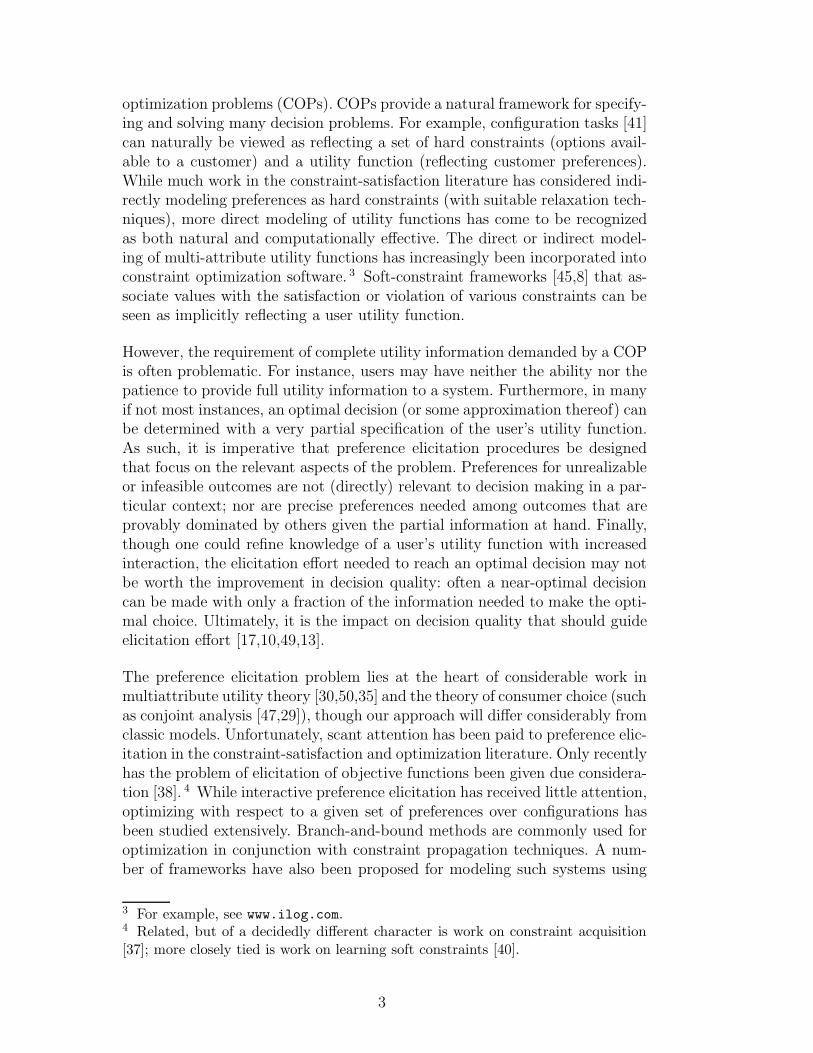
The constraint graph for a given set of constraints is the undirected graphwhose nodes are attributes and whose edges connect any two attributes thatoccur in the same constraint. This graph has useful properties that can be usedto determine the worst-case complexity of various algorithms for constraint-satisfaction and constraint-based optimization [20]. Figure 1 illustrates a smallconstraint graph over four variables induced by the logical constraints shown.

Our focus here will not be on constraint satisfaction, but rather on constraint-

6

based optimization problems (COPs). 5 Suppose we have a known non-negativeutility function u : Dom(X) → R+ which ranks all states (whether feasible ornot) according to their degree of desirability. 6 Our aim is to find an optimalfeasible state x∗; that is, any

x∗ ∈ arg maxx∈Feas(X)

u(x).

Since choices are restricted to feasible states, we sometimes call feasible statesdecisions. Without making any assumptions regarding the nature of the util-ity function (e.g., with regard to structure, independence, compactness, etc.)we can formulate the COP in an “explicit” fashion as a (linear) 0-1 integerprogram:

max{Ix,Xi}

∑x

uxIx subject to A and C, (1)

where we have:

• variables Ix: for each x ∈ Dom(X), Ix is a Boolean variable indicatingwhether x is the decision made (i.e., the feasible state chosen). In otherwords, Ix = 1 iff x is the solution to the COP.

• variables Xi: Xi is a Boolean variable corresponding to the ith attribute.In other words, variables Xi = 1 iff feature Xi is true in the solution to theCOP. 7

• coefficients ux: for each x ∈ Dom(X), constant ux denotes the (known)utility of state x.

• constraint set A: for each variable Ix, we impose a constraint that relatesit to its corresponding variable assignment. Specifically, for each Xi: if Xi

is true in x, we constrain Ix ≤ Xi; and if Xi is false in x, we constrainIx ≤ 1 − Xi. We use A to denote this set of state definition constraints.

• constraint set C: we impose each feasibility constraint C` on the attributesXi ∈ X[`]. Logical constraints on the variables Xi can be written in a naturalway as linear constraints [18], so we omit details. 8

Note that this formulation ensures that, if there is a feasible solution (giventhe constraints A and C), then exactly one Ix will be non-zero.

5 We use the term constraint-based optimization (often called constraint optimiza-tion) to refer to discrete combinatorial optimization problems with explicit logicalconstraints over variable instantiations, as in CSPs, to distinguish these from moregeneral constrained optimization problems with arbitrary (e.g., continuous) vari-ables and general functional constraints.6 For ease of presentation, we assume the utility function has been normalized tobe non-negative. Nothing critical depends on this, as such normalization is alwayspossible [23].7 If features are non-Boolean, then Xi simply needs to be a general integer variableranging over Dom(Xi).8 Again, generalizing the form of these constraints to generalized logical constraintsinvolving non-Boolean attributes is straightforward.

7

As an example of the interplay between the constraints in A and C, considerthe example in Figure 1. The following constraints will be present in the set Afor the state abcd (with analogous constraints for the other 15 instantiationsof the four Boolean variables):

Iabcd ≤ A; Iabcd ≤ B; Iabcd ≤ D; Iabcd ≤ 1 − D;

while the constraint set C, capturing the three domain constraints in the figureare:

A + B ≥ 1; B + C ≥ 1; A + B + C ≤ 2.

2.2 Factored Utility Models

Even with logically specified constraints, solving a COP in the manner aboveis not usually feasible, since the utility function is not specified concisely. As aresult, the IP formulation above is not practical, since there is one Ix variableper state and the number of states is exponential in the number of attributes.With such flat utility functions, it is not generally possible to formulate theoptimization problem concisely: indeed, if there is no (structural) relationshipbetween the utility of different states, little can be done but to enumeratefeasible states to ensure that an optimal solution is found. By contrast, if somestructure is imposed on the utility function, say, in the form of a factored (orgraphical) model, we are then often able to reduce the number of variables tobe linear in the number of parameters of the factored model.

We consider here generalized additive independence (GAI) models [22,3], anatural, but flexible and fully expressive generalization of additive (or linear)utility models. 9 GAI is appealing because of its generality and expressiveness;for instance, it encompasses both linear models [30] and UCP-nets [12] as spe-cial cases, 10 but can capture any utility function. The advantage of structuredutility models, and GAI specifically, is that the constraint-based optimiza-tion can be formulated and (typically) solved without explicit enumeration ofstates. While we focus on the GAI model, other compact structured utilitymodels can be exploited in similar fashion (e.g., see the many such modelsproposed by Keeney and Raiffa [30]).

The GAI model assumes that our utility function can be written as the sum

9 Fishburn [22] introduced the model, using the term interdependent value additiv-ity ; Bacchus and Grove [3] dubbed the same concept GAI, which seems to be morecommonly used in the AI literature currently.10 For example, UCP-nets encompass GAI with some additional restrictions. Henceany algorithm for GAI models automatically applies to UCP-nets, though one mightbe able to exploit the structure of UCP-nets for additional computational gain.

8

of K local utility functions, or factors, over small sets of attributes:

u(x) =∑k≤K

fk(x[k]). (2)

Here each function fk depends only on a local family of attributes X[k] ⊂X. We denote by x[k] the restriction of state x to the attributes in X[k].Again we assume that each function fk is non-negative. For example, if X ={A, B, C, D} we might decompose a utility function as follows:

u(ABCD) = f1(A, B) + f2(B, C).

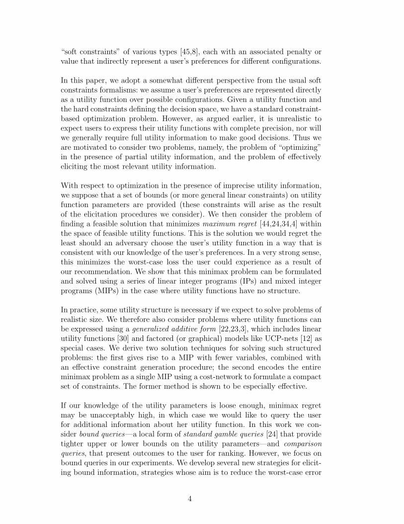
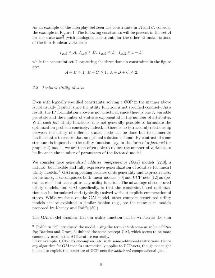
Figure 2 illustrates a possible instantiation of the two factors. Note that a userwith such a utility function exhibits no preference for the different values ofvariable D.

The conditions under which a GAI model provides an accurate representationof a utility function were defined by Fishburn [22,23]. We provide the intuitionshere. Let P be some probability distribution over Dom(X), interpreted asa gamble or lottery presented to the decision maker. For instance, P maycorrespond to the distribution over outcomes induced by some decision shecould take. Fishburn showed that the decision maker’s utility function u couldbe written in GAI form over factors fk iff she is indifferent between any pair ofgambles P and Q over Dom(X) whose marginals over each subset of variablesX[k] (k ≤ K) are identical. Note that GAI models are completely general(since any utility function can be represented trivially using a single factorconsisting of all variables). Furthermore, linear models are a special case inwhich we have a singleton factor for each variable.

We refer to a pair 〈C, {fk : k ≤ K}〉 as a structured COP, where C is a setof feasibility constraints and {fk : k ≤ K} is a set of utility factors. An IPsimilar to Eq. 1 can be used to solve for the optimal decision in the case of aGAI model:

max{Ix[k],Xi}

∑k≤K

∑x[k]∈Dom(X[k])

ux[k]Ix[k] subject to A and C. (3)

Instead of one variable Ix per state, we now have a set of local state vari-ables Ix[k] for each family k and each instantiation x[k] ∈ Dom(X[k]) of thevariables in that family. Similarly, we have one associated constant coefficientux[k] denoting fk(x[k]). Ix[k] is true iff the assignment to X[k] is x[k]. EachIx[k] is related logically to the attributes X ∈ X[k] by (local) state definitionconstraints A as before, and usual feasibility constraints C are also imposedas above.

Notice that the number of variables and constraints in this IP (excluding theexogenous feasibility constraints C) is now linear in the number of parame-

9

A B C

D

AB 15

AB 6

AB 10

AB 2

BC 13

BC 15

BC 5

BC 3

AB BC

Fig. 2. An example utility graph induced by the two utility factors shown to theleft.

ters of the underlying utility model, which itself is linear in the number ofattributes |X| if we assume that the size of each utility factor fk is bounded.This compares favorably with the exponential size of the IP for unfactoredutility models in Sec. 2.1.

This formulation of COPs is more or less the same as several other models ofCOPs found in the constraint satisfaction literature. For example, the notionof a cost network is often used to represent objective functions by assuming asimilar form of factored decomposition of the objective function [20]. Specif-ically, let the utility graph be defined in the same fashion as the constraintgraph, but with edges connecting attributes that occur in the same utilityfactor. This utility graph can be viewed as a cost network. Figure 2 illustratesthe utility graph over variables {A, B, C, D} induced by the utility functiondecomposition described above (corresponding to the two utility factors ABand BC shown at the left of the figure).

Similarly, certain soft constraint formalisms can be used [8]. Every constraintis assigned a cost corresponding to a penalty incurred if that constraint is notsatisfied. Hard constraints in C are assigned an infinite cost, and constraintscorresponding to configurations of local utility factors are given a finite costcorresponding to their (negative) utility. The goal is to find a minimum coststate, with the infinite costs associated with hard constraints ensuring a pref-erence for any feasible solution over any infeasible solution.

The IP formulation of structured COPs in Eq. 3 can be solved using off-the-shelf solution software for general IPs. Various special purposes algorithmsthat rely on the use of dynamic programming (e.g., the variable eliminationalgorithm) or constraint satisfaction techniques can also be used to solve theseproblems; we refer to Dechter [20] for a discussion of various algorithmic ap-proaches to COPs developed in the constraint satisfaction literature. Whilemany of these could be adapted to address the problems discussed in the pa-per, we will focus on IP formulations and their direct solution using standardIP software.

We remark here on the use of utility functions rather than (qualitative) prefer-

10

ence rankings in this work. In a deterministic setting, such as in the constraint-based framework adopted here, one does not need utility functions to makedecisions. Instead an ordinal preference ranking will suffice [30] since, with-out uncertainty, strength of preference information is not needed to assesstradeoffs: complete ordinal preference information will dictate which feasibleoutcome is preferred. However, in large multiattribute domains, even withfactored preference models, full elicitation will often be time-consuming andunnecessary. As discussed our aim is to make decisions with incomplete prefer-ence information. If we make a decision that is potentially suboptimal, we can-not be sure of its quality unless we have some information about the strengthof preference of this decision (at least relative to the optimal decision). Sim-ply knowing that one decision “may be preferred” to another does not give usenough information to know whether additional preference information shouldbe elicited if we are content with making good, rather than, optimal decisions.

3 Minimax Regret

In many circumstances, we are faced with a COP in which a user may nothave fully articulated her utility function over configurations of attributes.This arises naturally when distinct configurations must be produced for userswith different preferences, with some form of utility elicitation used to ex-tract only a partial expression of these preferences. It will frequently be thecase that we must make a decision before a complete utility function can bespecified. For instance, users may have neither the ability nor the patience toprovide full utility information to a system before requiring a decision to berecommended. Furthermore, in many if not most instances, an optimal deci-sion (or some approximation thereof) can be determined with a very partialspecification of the user’s utility function. This will become evident in ourpreference elicitation framework and the models we consider in this paper.

If the utility function is unknown, then we have a slightly different problemthan the standard COP. We cannot maximize utility (or expected utility instochastic decision problems) because the utility function is incompletely spec-ified. However, we will often have constraints on the utility function, eitherinitial information about plausible utility values, or more refined constraintsbased on the results of utility elicitation with a specific user. For example,these might be bounds on the parameters of the utility model, or possiblymore general constraints (as we discuss below). Given such a set of possibleutility functions (namely those consistent with these constraints), we mustadopt some suitable decision criterion for optimization, knowing only that theuser’s utility function lies within this set.

In the paper we propose the use of minimax regret [24,12,42,49] as a natural

11

decision criterion for imprecise COPs. We first define the notion of minimaxregret and then provide some motivation for its use as a suitable criterion inthis setting.

3.1 Minimax Regret in COPs

Minimax regret is a very natural criterion for decision making with impre-cise or incompletely specified utility functions. It requires that one adopt the(feasible) assignment x with minimum max regret, where max regret is thelargest amount by which one could regret making decision x (while allowingthe utility function to vary within the bounds). It has been suggested as analternative to classical expected utility theory. Specifically, it has been pro-posed as a means for accounting for uncertainty over possible states of nature(or the outcomes of decisions) [43,34,4], both when probabilistic informationis unavailable, and as a descriptive theory of human decision making that ex-plains certain common violations of von Neumann-Morgenstern [48] axioms.However, only recently has it been considered as a means for dealing with theutility function uncertainty a decision system may possess regarding a user’spreferences [12,42,49,14]. It is this formulation we present here.

Formally, let U denote the set of feasible utility functions, reflecting our par-tial knowledge of the user’s preferences. The set U may be finite; but morecommonly it will be continuous, defined by bounds (or constraints) on (setsof) utility values u(x) for various states. We refer to a pair 〈C,U〉 as an im-precise COP, where C is a set of feasibility constraints and U is the set offeasible utility functions. In the case where U is defined by a finite set of lin-ear constraints U , we sometimes abuse terminology by speaking of 〈C,U〉 asan imprecise COP.

We define minimax regret in stages:

Defn 1 The pairwise regret of state x with respect to state x′ over feasibleutility set U is defined as

R(x,x′,U) =maxu∈U

u(x′) − u(x). (4)

Intuitively, U represents the knowledge a decision support system has of theuser’s preferences. R(x,x′,U) is the most the system could regret choosing xinstead of x′, if an adversary could impose any utility function in U on theuser. In other words, if the system were forced to choose between x and x′,then this corresponds to the worst-case loss associated with choosing x ratherthan x′ with respect to possible realizations of u ∈ U.

12

A B C

D

AB [9,17]

AB [5,8]

AB [10,11]

AB [0,3]

BC [2,4]

BC [0,10]

BC [4,8]

BC [0,5]

AB BC

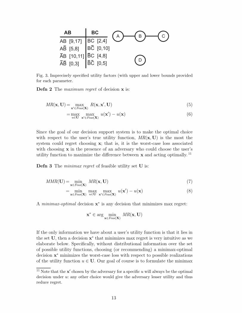
Fig. 3. Imprecisely specified utility factors (with upper and lower bounds providedfor each parameter.

Defn 2 The maximum regret of decision x is:

MR(x,U)= maxx′∈Feas(X)

R(x,x′,U) (5)

= maxu∈U

maxx′∈Feas(X)

u(x′) − u(x) (6)

Since the goal of our decision support system is to make the optimal choicewith respect to the user’s true utility function, MR(x,U) is the most thesystem could regret choosing x; that is, it is the worst-case loss associatedwith choosing x in the presence of an adversary who could choose the user’sutility function to maximize the difference between x and acting optimally. 11

Defn 3 The minimax regret of feasible utility set U is:

MMR(U) = minx∈Feas(X)

MR(x,U) (7)

= minx∈Feas(X)

maxu∈U

maxx′∈Feas(X)

u(x′) − u(x) (8)

A minimax-optimal decision x∗ is any decision that minimizes max regret:

x∗ ∈ arg minx∈Feas(X)

MR(x,U)

If the only information we have about a user’s utility function is that it lies inthe set U, then a decision x∗ that minimizes max regret is very intuitive as weelaborate below. Specifically, without distributional information over the setof possible utility functions, choosing (or recommending) a minimax-optimaldecision x∗ minimizes the worst-case loss with respect to possible realizationsof the utility function u ∈ U. Our goal of course is to formulate the minimax

11 Note that the x′ chosen by the adversary for a specific u will always be the optimaldecision under u: any other choice would give the adversary lesser utility and thusreduce regret.

13

regret optimization (Eq. 8) in a computationally tractable way. We addressthis in Section 4.

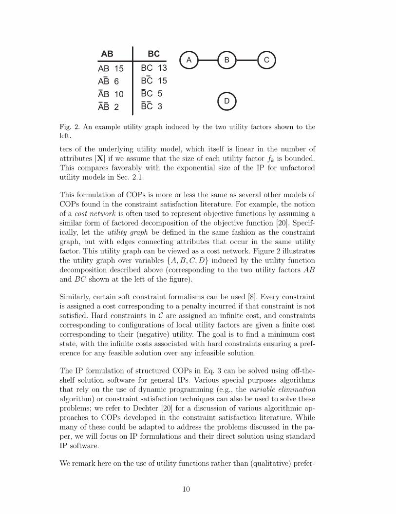
To illustrate minimax regret, consider the example illustrated in Figures 1and 2; but suppose that the precise utility values associated with these factorsare unknown, and instead replaced with the upper and lower bounds shownin Figure 3. The problem admits five feasible states, and the pairwise maxregret R(x,x′,U) for each pair of states (with x along columns and x′ alongthe rows) is shown in the following table:

ABC ABC ABC ABC ABC Max Regret

ABC 0 8 5 2 10 10

ABC 4 0 7 6 2 7

ABC 12 18 0 6 12 18

ABC 7 15 6 4 0 15

ABC 15 7 6 4 0 15

The max regret of each feasible state is shown in the final column, from whichwe see that state ABC is the minimax optimal decision.

3.2 Motivation for Minimax Regret

As mentioned, minimax regret has been widely studied (and critiqued) as ameans for decision making under uncertainty. It has been studied primarilyas a means for making decisions when a decision maker is unwilling or un-able to quantify her uncertainty over possible states of nature, or as a meansof explaining violations of classical axioms of expected utility theory. Savage[43] introduced the notion though could not provide a “categorical” defenseof its use. The use of regret, including the incorporation of feelings of regret(and its opposite, “rejoicing”) into expected utility theory, has been proposedas a means of accounting for the manner in which people violate the axiomsof expected utility theory in practice [34,4]. Difficulties with the use of thisdecision criterion include the fact the minimax regret criterion does not sat-isfy the principle of irrelevant alternatives [43,24], and regret theory fails tosatisfy a reasonable notion of stochastic dominance [39]. It can also be arguedthat, from a Bayesian perspective, a decision maker might as well constructtheir own subjective assessment of possible states of nature. For this reason,minimax regret is often viewed as too cautious a criterion.

The perspective we adopt here is somewhat different. We do not adopt mini-

14

max regret as a means of accounting for a decision maker’s personal feelingsof regret. Rather we define regret with respect to our decision system’s uncer-tainty with respect to the user’s true utility function. It seems incontrovertiblethat there will generally be some such utility function uncertainty on the partof any system designed to make decisions on behalf of users. The only issue ishow this uncertainty is represented and reasoned with.

Naturally, Bayesian methods may be entirely appropriate in some circum-stances: if one can quantify uncertainty over possible utility functions proba-bilistically, then one can take expectations over this density to determine theexpected expected utility of a decision [17,10,11]. However, there are manycircumstances in which the Bayesian approach is inappropriate. First, it canoften be very difficult to develop reasonable priors over the utility functionsof a wide class of users. Furthermore, representing priors over such complexentities as utility functions is fraught with difficulty and inevitably requirescomputational approximations in inference (this is made abundantly clear inrecent Bayesian approaches to preference elicitation [17,10]). As a consequence,the value of such “normatively correct” models is undermined in practice. Of-ten bounds on the parameters of utility functions are generally much easierto come by, much easier to maintain, and lend themselves to much more com-putationally manageable algorithms as we will see in this paper. In addition,max regret provides an upper bound on the average loss when probabilisticinformation is known. As we will see below, minimax regret is a very effectivedriver of preference elicitation, so concerns about its pessimistic nature seemunfounded here. We will see that with relatively few queries, max regret can bereduced to very low levels (often with provably optimal solutions). Though wedon’t pursue this approach here, when probabilistic information is available,it can be combined rather effectively with minimax computation [49].

Finally, it is worth noting that making a recommendation whose utility isnear optimal in expectation, as is the case in Bayesian models of preferenceelicitation, is often of cold comfort to a user when the decision made is actuallyvery far from optimal. While minimax regret provides a worst-case bound onthe loss in decision quality arising from utility function uncertainty (even incases where distributional information is available), Bayesian methods cannottypically provide such a bound. In some contexts, such as procurement, thishas been reported as a source of contention with clients using automatedpreference elicitation [14]. The argument is often made that users do not wantto “leave money on the table” (even if the odds are low); if any money is lefton the table, they want guarantees (as opposed to probabilistic assurances)that the amount they could have saved through further preference elicitationis limited.

Recently, a considerable amount of work in robust optimization has adopted

15

the minimax regret decision criterion [32,1,2]. 12 This work addresses com-binatorial optimization problems with data uncertainty (e.g., shortest pathproblems or facility location with uncertain parameters) and find “robust devi-ation decisions” that minimize max regret. While the perspective in this workis somewhat different than that adopted in ours, the models and methods arequite similar. Our formulation is specific to the constraint-based optimizationsetting, but more importantly we focus on how minimax regret can be usedto drive the process of elicitation, a problem not addressed systematically inthe robust optimization literature. Our techniques, apart from preference elic-itation, could be adapted for problems in robust optimization as a means todrive the reduction in data uncertainty.

4 Computing Minimax Regret in COPs

We address the computational problem of computing minimax optimal deci-sions in several stages. We initially assume upper and lower bounds on utilityparameters and discuss procedures for minimax computation for this form ofuncertainty. We begin in Sec. 4.1 by formulating minimax regret in flat (unfac-tored) utility models to develop intuitions used in the factored case. In Sec. 4.2we discuss the computation of maximum regret in factored utility models, andpropose two procedures for dealing with minimax regret. We evaluate one ofthese methods empirically in Sec. 4.3. Finally, in Sec. 4.4 we propose a gener-alization for the minimax problem in the case where the feasible utility set isdefined by arbitrary linear constraints on parameters of the utility model.

4.1 Minimax Regret with Flat Utility Models

If we make no assumptions about the structure of the utility function, nor anyassumptions about the nature of the feasible utility set U, the optimizationproblem defined in Eq. 8 can be posed directly as a semi-infinite, quadratic,mixed-integer program (MIP):

min{Mx,Ix,Xi}

∑x

MxIx subj. to

Mx ≥ ux′ − ux ∀x ∈ X, ∀ x′ ∈ Feas(X), ∀ u ∈ U

A and C

where we have:

• variables Mx: for each x, Mx is a real-valued variable denoting the maxregret when decision x is made (i.e., when that state is chosen).

12 The term “robust optimization” has a number of different interpretations (see forexample the work of Ben-Tal and Nemirovski [5]).

16

• variables Ix: for each x, Ix is a Boolean variable indicating whether x is thedecision made.

• coefficients ux: for each u ∈ U and each state x, ux denotes the utility of xgiven utility function u.

• state definition constraints A and feasibility constraints C (defined as above).

Direct solution of this MIP is problematic, specifically because of the set ofconstraints on the Mx variables. First, if U is continuous (the typical casewe consider here), then the set of constraints of the form Mx ≥ ux′ − ux isalso continuous, since it requires that we “enumerate” all utility values ux andux′ corresponding to any utility function u ∈ U. Furthermore, it is criticalthat we restrict our attention to those constraints associated with x′ in thefeasible set (i.e., those states satisfying C). Fortunately, we can often tacklethis seemingly complex optimization in much simpler stages if we make somevery natural assumptions regarding the nature of the feasible utility space andutility function structure.

We begin by considering the case where our imprecise knowledge regardingall utility parameters ux is independent and represented by simple upper andlower bounds. For example, asking standard gamble queries, as discussed fur-ther in Sec. 5.1, provides precisely such bounds on utility values [24]. Specifi-cally, we assume an upper bound ux↑ and a lower bound ux↓ on each ux, thusdefining the feasible utility set U to be a hyperrectangle. This assumptionallows us to compute the minimax regret in three simpler stages, which wenow describe. 13

First, we note that the pairwise regret for an ordered pair of states can beeasily computed since each ux is bounded by an upper and lower bound:

R(x,x′,U) =

u′x↑ - ux↓ when x 6= x′

0 when x = x′(9)

Let rx,x′ denote this pairwise regret value for each x, x′, which we now assumehas been pre-computed for all pairs.

Second, using Eq. 5, we can also compute the max regret MR(x,U) of anystate x based on the pre-computed pairwise regret values rx,x′. Specifically,we can enumerate all feasible states x′, retaining the largest (pre-computed)pairwise regret:

MR(x,U) = maxx′∈Feas(X)

rx,x′. (10)

13 This transformation essentially reduces the semi-infinite quadratic MIP to a finitelinear IP.

17

Alternatively, we can search through feasible states “implicitly” with the fol-lowing IP:

MR(x,U) = max{Ix′ ,X′

i}

∑x′

rx,x′Ix′ subject to A and C. (11)

Third, let mx denote the value of MR(x,U). With the max regret terms mx =MR(x,U) in hand, we can compute the minimax regret MMR(U) readily. Wesimply enumerate all feasible states x and retain the one with the smallest(precomputed) max regret value mx:

MMR(U) = minx∈Feas(X)

mx. (12)

Again, this enumeration may be done implicitly using the following IP:

MMR(U) = min{Ix,Xi}

∑x

mxIx subject to A and C. (13)

In this flat model case, the two IPs above are not necessarily practical, sincethey require one indicator variable per state. However, this reformulation doesshow that the original quadratic MIP with a continuous set of constraints canbe solved in stages using finite, linear IPs. More importantly, these intuitionswill next be applied to develop an analogous procedure for factored utilitymodels.

Note that the strategy above hinges on the fact that we have independentlydetermined upper and lower bounds on the utility value of each state. If utilityvalues are correlated by more complicated constraints, this strategy will notgenerally work. In particular, comparison queries in which a user is askedwhich of two states is preferred induce linear constraints on the entire set ofutility parameters, thus preventing exploitations of independent upper andlower bounds. We discuss formulations that allow us to deal with such feasibleutility sets in Sec. 4.4. However, we initially focus on the case of independentbounds.

4.2 Minimax Regret with Factored Utility Models

The optimization for flat models is interesting in that it allows us to get a goodsense of how minimax regret works in a constraint-satisfaction setting. From apractical perspective, however, the above model has little to commend it. Bysolving IPs with one Ix variable per state, we have lost all of the advantage ofusing a compact and natural constraint-based approach to problem modeling.As we have seen when optimizing with known utility functions, if there is noa priori structure in the utility function, there is very little one can do but

18

enumerate (feasible) states. On the other hand, when the problem structureallows for modeling via factored utility functions the optimization becomesmore practical. We now show how much of this practicality remains when ourgoal is to compute the minimax-optimal state given uncertainty in a factoredutility function represented as a graphical model.

Assume a set of factors fk, k ≤ K, defined over local families X[k], as de-scribed in Sec. 2.2. The parameters of this utility function are denoted byux[k] = fk(x[k]), where x[k] ranges over Dom(X[k]). We use the term impre-cise structured COP to describe an imprecise COP 〈C,U〉 where the feasibleutility set U is defined by a set of constraints U over the parameters ux[k] ofa factored utility model {fk : k ≤ K}.

As in the flat-model case, we assume upper and lower bounds on each ofthese parameters, which we denote by ux[k]↑ and ux[k]↓, respectively. Hence therange of each utility factor fk for a given assignment x[k] corresponds to aninterval. By defining u(x) as in Eq. 2, pairwise regret, max regret and minimaxregret are all defined in the same manner outlined in Sec. 3. We now showhow to compute each of these quantities in turn by generalizing the intuitionsdeveloped for flat models.

4.2.1 Computing Pairwise Regret and Max Regret

As in the unfactored case (Sec. 4.1), it is straightforward to compute thepairwise regret of any pair of states x and x′. For each factor fk and pair oflocal assignments x[k],x′[k], we define the local pairwise regret :

rx[k],x′[k] =

ux′[k]↑ − ux[k]↓ when x[k] 6= x′[k]

0 when x[k] = x′[k]

With factored models it is not hard to see from Eq. 2 and Eq. 9 that R(x,x′,U)is simply the sum of local pairwise regrets:

R(x,x′,U) =∑k

rx[k],x′[k]. (14)

We can compute max regret MR(x,U) by substituting Eq. 14 into Eq. 5:

MR(x,U) = maxx′∈Feas(X)

∑k

rx[k],x′[k], (15)

which leads to the following IP formulation:

MR(x,U) = max{Ix′[k],X

′i}

∑k

∑x′[k]

rx[k],x′[k]Ix′[k] subject to A and C. (16)

19

The above IP differs from its flat counterpart (Eq. 11) in the use of oneindicator variable Ix′[k] per utility parameter rather than one per state, andis thus much more compact and efficiently solvable. Indeed, the size of the IPin terms of the number of variables and constraints (excluding exogenouslydetermined feasibility constraints C) is linear in the size of the underlyingfactored utility model.

4.2.2 Computing Minimax Regret: Constraint Generation

We can compute minimax regret MMR(U) by substituting Eq. 15 into Eq. 7:

MMR(U) = minx∈Feas(X)

maxx′∈Feas(X)

∑k

rx[k],x′[k] (17)

which leads to the following MIP formulation:

MMR(U) = min{Ix[k],Xi}

maxx′∈Feas(X)

∑k

∑x[k]

rx[k],x′[k]Ix[k] subject to A and C (18)

= min{Ix[k],Xi,M}

M

subject to

M ≥ ∑k

∑x[k] rx[k],x′[k]Ix[k] ∀x′ ∈ Feas(X)

A and C(19)

In Eq. 18, we introduce the variables for the minimization, while in Eq. 19we transform the minimax program into a min program. The new real-valuedvariable M corresponds to the max regret of the minimax-optimal solution.In contrast with the flat IP (Eq. 13), this MIP has a number of Ix[k] variablesthat is linear in the number of utility parameters. However, this MIP is notgenerally compact because Eq. 19 has one constraint per feasible state x′.Nevertheless, we can get around the potentially large number of constraintsin either of two ways.

The first technique we consider for dealing with the large number of constraintsin Eq. 19 is constraint generation, a common technique in operations researchfor solving problems with large numbers of constraints. Our approach can beviewed as a form of Benders’ decomposition [6,36]. This approach proceeds byrepeatedly solving the MIP in Eq. 19, but using only a subset of the constraintson M associated with the feasible states x′. At the first iteration, all constraintson M are ignored. At each iteration, we obtain a solution indicating somedecision x with purported minimax regret; however, since certain unexpressedconstraints may be violated, we cannot be content with this solution. Thus,we look for the unexpressed constraint on M that is maximally violated bythe current solution. This involves finding a witness x′ that maximizes regretw.r.t. the current solution x ; that is, a decision x′ (and, implicitly, a utility

20

function) that an adversary would choose to cause a user to regret x the most.

Recall that finding the feasible x′ that maximizes R(x,x′,U) involves solvinga single IP given by Eq. 16. We then impose the specific constraint associatedwith witness x′ and re-solve the MIP in Eq. 19 at the next iteration with thisadditional constraint. Formally, we have the following procedure:

(1) Let Gen = {x′} for some arbitrary feasible x′.(2) Solve the MIP in Eq. 19 using the constraints corresponding to states in

Gen. Let x∗ be the MIP solution with objective value m∗.(3) Compute the max regret of state x∗ using the IP in Eq. 16, producing

a solution with regret level r∗ and adversarial state x′′. If r∗ > m∗, thenadd x′′ to Gen and repeat from Step 2; otherwise (if r∗ = m∗), terminatewith minimax-optimal solution x∗ (with regret level m∗).

Intuitively, when we solve the MIP in Step 2 using only the constraints inGen, we are computing minimax regret against a restricted adversary : theadversary is only allowed to use choices x′ ∈ Gen in order to make use regretour solution x∗ to the MIP. As such, this solution provides a lower bound ontrue minimax regret (i.e., the solution that would have been obtained were acompletely unrestricted adversary considered).

When we compute the true max regret r∗ of x∗ in Step 3, we also obtainan upper bound on minimax regret (since we can always attain max regretof r∗ simply by stopping and recommending solution x∗). It is not hard tosee that if r∗ = m∗, then no constraint is violated at the current solutionx∗ (and our upper and lower bounds on minimax regret coincide); so x∗ isthe minimax-optimal configuration at this point. The procedure is finite andguaranteed to arrive at the optimal solution. The constraint generation routineis not guaranteed to finish before it has the full set of constraints, but it isrelatively simple and (as we will see) tends to generate a very small numberof constraints. Thus in practice we solve this very large MIP using a seriesof small MIPs, each with a small number of variables and a set of activeconstraints that is also, typically, very small.

Since minimax regret will be computed between elicitation queries, it is criticalthat minimax regret be estimated in a relatively short period of time (e.g., fiveseconds for certain applications, five minutes for others, possibly several hoursfor very high stakes applications). With this in mind, several improvementscan be made to speed up minimax regret computation. For instance, it is oftensufficient to find a feasible (instead of optimal) configuration x for the MIP inEq. 19 for each newly generated constraint. Intuitively, as long as the feasiblex allows us to find a violated constraint, the constraint generation continuesto progress. Hence, instead of waiting a long time for an optimal x, we canstop the MIP solver as soon as we find a feasible solution for which a violated

21

constraint exists. Of course, at the last iteration, when there are no violatedconstraints, we have no choice but to wait for the optimal x.

Minimax regret can also be estimated more quickly—to allow for the real-time response needed for interactive optimization—by exploiting the anytimenature of the computation to simply stop early. Since minimax regret is com-puted incrementally by generating constraints, early stopping has the effectthat some violated constraints may not have been generated. As a result thesolution provides us with a lower bound on minimax regret. We can terminatedepending early based on a fixed number of iterations (constraints), a fixedamount of computation time, or by terminating when bounds on the solutionare tight enough. Apart from this lower bound, we can also obtain an upperbound on minimax regret by computing the max regret of the x found for thelast minimax MIP solved. Note that we may need to explicitly compute thissince Step (3) of our procedure may not be invoked if we terminate based onlyon the number of iterations rather than testing for constraint violation.

Approximation can be very appealing if real-time interactive response is re-quired. The anytime flavor of the algorithm means that these lower and upperbounds are often tight enough to provide elicitation guidance of similar qualityto that obtained from computing minimax regret exactly.

Although the full interaction of minimax regret computation with elicitationis explored in Sec. 5, as a precursor to that discussion, we mention anotherstrategy for accelerating computation which directly influences the queryingprocess. We have observed, unsurprisingly, that the minimax regret problemsolved after receiving a response to one query is very similar to that solvedbefore posing the query. As such, one can “seed” the minimax procedure in-voked after a query with the constraints generated at the previous step. In thisway, typically, only a few extra constraints are generated during each minimaxcomputation. Given that the running time of minimax regret is dominated byconstraint generation, this effectively amortizes the cost of minimax compu-tation over a number of queries.

4.2.3 Computing Minimax Regret: A Cost Network Formulation

A second technique for dealing with the large number of constraints in Eq. 19is to use a cost network to generate a compact set of constraints that effec-tively summarizes this set. This type of approach has been used recently, forexample, to solve Markov decision processes [26]. The main benefit of the costnetwork approach is that, in principle, it allows us to formulate a MIP witha feasible number of constraints (as elaborated below). We have observed,however, the constraint generation approach described above is usually muchfaster in practice and much easier to implement, even though it lacks the same

22

worst-case run-time guarantees. Indeed, this same fact has been observed inthe context of MDPs [46]. It is for this reason that we emphasize (and onlyexperiment with) the constraint generation algorithm. However, we sketch thecost network formulation for completeness.

To formulate a compact constraint system, we first transform the MIP ofEq. 19 into the following equivalent MIP by introducing penalty terms ρx[`]

for each feasibility constraint C`:

MMR(U) = min{Ix[k],Xi,M}

M

subject to

M ≥ ∑k

∑x[k] rx[k],x′[k]Ix[k] +

∑` ρx′[`] ∀x′ ∈ Dom(X)

A and C

= min{Ix[k],Xi,M}

M

subject to

M ≥ ∑k Rx′[k] +

∑` ρx′[`] ∀x′ ∈ Dom(X)

Rx′[k] =∑

x[k] rx[k],x′[k]Ix[k] ∀k,x′[k] ∈ Dom(X[k])

A and C

(20)

The MIP of Eq. 19 has one constraint on M per feasible state x′, whereas theMIP of Eq. 20 has one constraint per state x′ (whether feasible or not). There-fore, to effectively maintain the feasibility constraints on x′, we add penaltyterms ρx′[`] that make a constraint on M meaningless when its correspond-ing state x′ is infeasible. This is achieved by defining a local penalty functionρ`(x′[`]) for each logical constraint C` that returns −∞ when x′[`] violates C`

and 0 otherwise.

This transformation has, unfortunately, increased the number of constraints.However, it in fact allows us to rewrite the constraints in a much more compactform, as follows. Instead of enumerating all constraints on M , we analyticallyconstruct the constraint that provides the greatest lower bound, while simplyignoring the others. This greatest lower bound GLB is computed by takingthe max of all constraints on M :

GLB =maxx′

∑k

Rx′[k] +∑

`

ρx′[`]

=maxx′1

maxx′2

. . .maxx′

N

∑k

Rx′[k] +∑

`

ρx′[`].

This maximization can be computed efficiently by using variable elimina-tion [19], a well-known form of non-serial dynamic programming [7]. The idea

23

is to distribute the max operator inward over the summations, and then col-lect the results as new terms which are successively pulled out. We illustrateits workings by means of an example.

Suppose we have the attributes X1, X2, X3, X4, a utility function decomposedinto the factors f1(x1, x2), f2(x2, x3), f3(x1, x4) and two logical constraintswith associated penalty functions ρ1(x1) and ρ2(x3, x4). We then obtain

GLB =maxx′1

maxx′2

maxx′3

maxx′4

Rx′1,x′

2+ Rx′

2,x′3+ Rx′

1,x′4+ ρx′

1+ ρx′

3,x′4

=maxx′1

[ρx′1+ max

x′2

[Rx′1,x′

2+ max

x′3

[Rx′2,x′

3+ max

x′4

[Rx′1,x′

4+ ρx′

3,x′4]]]]

by distributing the individual max operators inward over the summations. Tocompute the GLB, we successively formulate new terms that summarize theresult of completing each max in turn, as follows:

Let Ax′1,x′

3= max

x′4

Rx′1,x′

4+ ρx′

3,x′4.

Let Ax′1,x′

2= max

x′3

Rx′2,x′

3+ Ax′

1,x′3.

Let Ax′1

= maxx′2

Rx′1,x′

2+ Ax′

1,x′2.

Let GLB = maxx′1

ρx′1+ Ax′

1.

Notice that this incremental procedure can be substantially faster than enu-merating all states x′. In fact the complexity of each step is only exponentialin the local subset of attributes that indexes each auxiliary A variable.

Based on this procedure, we can substitute all the constraints on M in theMIP in Eq. 20 with the following compact set of constraints that analyticallyencodes the greatest lower bound on M :

Ax′1,x′

3≥ Rx′

1,x′4+ ρx′

3,x′4

∀x′1, x

′3, x

′4 ∈ Dom(X1, X3, X4)

Ax′1,x′

2≥ Rx′

2,x′3+ Ax′

1,x′3

∀x′1, x

′2, x

′3 ∈ Dom(X1, X2, X3)

Ax′1≥ Rx′

1,x′2+ Ax′

1,x′2

∀x′1, x

′2 ∈ Dom(X1, X2)

M ≥ ρx′1+ Ax′

1∀x′

1 ∈ Dom(X1)

By encoding constraints in this way, the constraint system specified by theMIP in Eq. 20 can be generally encoded with a small number of variables

24

and constraints. Overall we obtain a MIP where: the number of Ix variables islinear in the number of parameters of the utility function; and the number ofauxiliary variables (the A variables in our example) and constraints that areadded is locally exponential with respect to the largest subset of attributesindexing some auxiliary variable. In practice, since this largest subset is oftenvery small compared to the set of all attributes, the resulting MIP encodingis compact and readily solvable. In particular, let the joint graph be the unionof the constraint graph and the utility graph (e.g., the union of the graphs inFigures 1 and 2). The complexity of this algorithm and hence the size of theresultant set of constraints is determined directly by the properties of variableelimination, and as such depends on the order in which the variables in Xare eliminated. More precisely, it is exponential in the tree width of the jointgraph induced by the elimination ordering [19]. Often this tree width is verysmall, thus rendering the algorithm only locally exponential [19].

4.3 Empirical Results

To test the plausibility of minimax regret computation, we implemented theconstraint generation strategy outlined above and ran a series of experimentsto determine whether factored structure was sufficient to permit practical so-lution times. We implemented the constraint generation approach outlined inSec. 4.2 and used CPLEX 7.1 as the generic IP solver. 14 Our experiments con-sidered two realistic domains—car rentals and real estate—as well as randomlygenerated synthetic problems. In each case we imposed a factored structure toreduce the required number of utility parameters (upper and lower bounds).

For the real-estate problem, we modeled the domain with 20 (multivalued)variables that specify various attributes of single family dwellings that are nor-mally relevant to making a purchase decision. The variables we used included:square footage, age, size of yard, garage, number of bedrooms, etc. Variableshad domains of sizes from XXX to XXX. In total, there were 47,775,744 pos-sible configurations of the variables. We then used a factored utility modelconsisting of 29 local factors, each defined on only one, two or three variables.In total, there were 160 utility parameters (i.e., utilities for local configura-tions). Therefore a total of 320 upper and lower bounds had to be specified, asignificant reduction over the nearly 108 values that would have been requiredusing a unfactored model. The local utility functions represented complemen-tarities and substitutabilities in the utility function, such as requiring a largeyard and a fence to allow a pool, sacrificing a large yard if the house happensto be near a park, etc.

14 These experiments were performed using a slightly older code base than that usedin the next section, on 2.4GHz PCs.

25

The car-rental problem features 26 multi-valued variables encoding attributesrelevant to consumers considering a car rental, such as: automobile size andclass, manufacturer, rental agency, seating and luggage capacity, safety fea-tures (air bags, ABS, etc.), and so on. of sizes from XXX to XXX. The totalnumber of possible variable configurations is 61,917,360,000. There are 36 localutility factors, each defined on at most five variables, giving rise to 435 util-ity parameters. Constraints encode infeasible configurations (e.g., no luxurysedans have four-cylinder engines).

For both the car-rental and real-estate problems, we first computed the con-figuration with minimax regret given manually chosen bounds on the utilityfunctions. The constraint generation technique of Sec. 4.2 took 40 seconds forthe car-rental problem and two seconds for the real-estate problem. It is in-teresting to note that only seven constraints (out of 61,917,360,000 possibleconstraints) for the car-rental problem and seven constraints (out of 47,775,744possible constraints) for the real-estate problem were generated to find an op-timal configuration. The structure exhibited by the utility functions of eachproblem is largely responsible for this small number of required constraints.

In practice, minimax regret computation will be interleaved with some pref-erence elicitation technique (as we discuss in Sec. 5). As the bounds on utilityparameters get tighter, we would like to know the impact on the running timeof our constraint generation algorithm. To that effect, we carried out an exper-iment where we randomly set bounds, but with varying degrees of tightness.Initial utility gaps (i.e., difference between upper and lower bounds) rangedfrom XXXXXXX. Figures 4 and 5 show how tightening the bounds decreasesthe running time in an exponential fashion, as well as the number of con-straints generated. For this experiment, bounds on utility were generated atrandom, but the difference between the upper and lower bounds of any utilitywas capped at a fixed percentage of some predetermined range. Intuitively, aspreferences are elicited, the values will shrink relative to the initial range.

Figures 4 and 5 show scatterplots of computation time and number of con-straints for ten random problem instances generated for each of a number ofincreasingly tight relative utility ranges. As those figures suggest, a significantspeed up is obtained as elicitation converges to the true utilities. Intuitively,the optimization required to compute minimax regret benefits from tighterbounds since some configurations emerge as clearly dominant, which in turnrequires the generation of fewer constraints.

We carried out a second experiment with synthetic problems. A set of ran-dom problems of varying sizes was constructed by randomly setting the utilitybounds as well as the variables on which each utility factor depends. Each util-ity factor depends on at most three variables and each variable has at mostfive values. Figure 6 shows the results as we vary the number of variables

26

100% 90% 80% 70% 60% 50% 40% 30% 20% 10%0.1

1

10

100

1,000

Relative utility range

Tim

e (s

econ

ds)

100% 90% 80% 70% 60% 50% 40% 30% 20% 10%1

10

100

1,000

Relative utility range

Num

ber

of c

onst

rain

ts g

ener

ated

Fig. 4. Computation time (left) and number of constraints generated (right) forminimax regret on real-estate problem (48 million configurations) as a function ofthe tightness of the utility bounds.

70% 60% 50% 40% 30% 20% 10%10

100

1,000

10,000

Relative utility range

Tim

e (s

econ

ds)

70% 60% 50% 40% 30% 20% 10%1

10

100

1,000

Relative utility range

Num

ber

of c

onst

rain

ts g

ener

ated

Fig. 5. Computation time (left) and number of constraints generated (right) forminimax regret on car-rental problem (62 billion configurations) as a function ofthe tightness of the utility bounds.

and factors (the number of factors is always the same as the number of vari-ables). The running time and the number of constraints generated increasesexponentially with the size of the problem. Note however that the number ofconstraints generated is still a tiny fraction of the total number of possibleconstraints. For problems with 10 variables, only 8 constraints were neces-sary (out of 278,864) on average; and for problems with 30 variables, only 47constraints were necessary (out of 2.8 × 1016) on average.

We also tested the impact of the relative tightness of utility bounds on the ef-ficiency of our constraint generation technique, with results shown in Figure 7.Here, problems of 30 variables and 30 factors were generated randomly whilevarying the relative range of the utilities with respect to some predeterminedrange. Each factor has at most three variables chosen randomly and each

27

10 12 14 16 18 20 22 24 26 28 300.1

1

10

100

1,000

10,000

Number of variables

Tim

e (s

econ

ds)

10 12 14 16 18 20 22 24 26 28 301

10

100

1,000

Number of variables

Num

ber

of c

onst

rain

ts g

ener

ated

Fig. 6. Computation time (left) and number of constraints generated (right) forartificial random problems as a function of problem size (number of variables andfactors).

100% 90% 80% 70% 60% 50% 40% 30% 20% 10%1

10

100

1,000

10,000

Relative utility range

Tim

e (s

econ

ds)

100% 90% 80% 70% 60% 50% 40% 30% 20% 10%1

10

100

1,000

Relative utility range

Num

ber

of c

onst

rain

ts g

ener

ated

Fig. 7. Computation time (left) and number of constraints generated (right) forminimax regret on artificial random problems (30 variables, 30 factors) as a functionof the tightness of the utility bounds.

variable can take at most five values. Once again, as the bounds get tighter,some configurations emerge as clearly dominant, which allows an exponentialreduction in the running time as well as the number of required constraints.

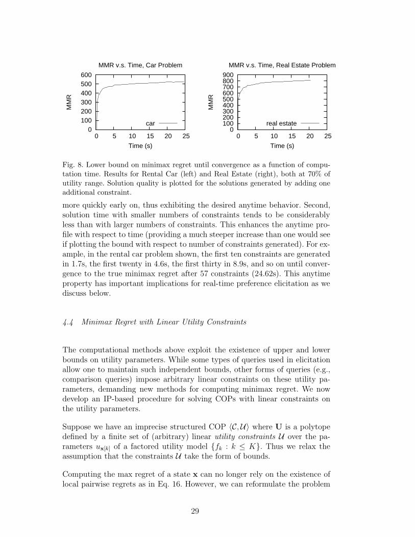
Finally, we illustrate the anytime properties of our algorithm. In Figure 8 weshow the lower bound on minimax regret as a function of computation time.Each data point corresponds to one additional generated constraint. As we cansee, the constraint generation algorithm has very good anytime properties, ap-proaching the true minimax regret level very quickly as a function of time andnumber of constraints. This is due to two factors. First, as a function of thenumber of constraints generated, minimax regret lower bounds increase much

28

0 100 200 300 400 500 600

0 5 10 15 20 25

MM

R

Time (s)

MMR v.s. Time, Car Problem

car 0

100 200 300 400 500 600 700 800 900

0 5 10 15 20 25

MM

R

Time (s)

MMR v.s. Time, Real Estate Problem

real estate

Fig. 8. Lower bound on minimax regret until convergence as a function of compu-tation time. Results for Rental Car (left) and Real Estate (right), both at 70% ofutility range. Solution quality is plotted for the solutions generated by adding oneadditional constraint.

more quickly early on, thus exhibiting the desired anytime behavior. Second,solution time with smaller numbers of constraints tends to be considerablyless than with larger numbers of constraints. This enhances the anytime pro-file with respect to time (providing a much steeper increase than one would seeif plotting the bound with respect to number of constraints generated). For ex-ample, in the rental car problem shown, the first ten constraints are generatedin 1.7s, the first twenty in 4.6s, the first thirty in 8.9s, and so on until conver-gence to the true minimax regret after 57 constraints (24.62s). This anytimeproperty has important implications for real-time preference elicitation as wediscuss below.

4.4 Minimax Regret with Linear Utility Constraints

The computational methods above exploit the existence of upper and lowerbounds on utility parameters. While some types of queries used in elicitationallow one to maintain such independent bounds, other forms of queries (e.g.,comparison queries) impose arbitrary linear constraints on these utility pa-rameters, demanding new methods for computing minimax regret. We nowdevelop an IP-based procedure for solving COPs with linear constraints onthe utility parameters.

Suppose we have an imprecise structured COP 〈C,U〉 where U is a polytopedefined by a finite set of (arbitrary) linear utility constraints U over the pa-rameters ux[k] of a factored utility model {fk : k ≤ K}. Thus we relax theassumption that the constraints U take the form of bounds.

Computing the max regret of a state x can no longer rely on the existence oflocal pairwise regrets as in Eq. 16. However, we can reformulate the problem

29

somewhat differently to allow this to be solved linearly even when the con-straints U take this more general form. First, we can recast the computationof max regret as a quadratic optimization:

MR(x,U) = max{Ix′[k],X

′i,Ux[k]}

∑k

[∑x′[k]

Ux′[k]Ix′[k]] − Ux[k] subject to A, C, and U(21)

We have introduced one real-valued variable Ux[k] (denoted Ux′[k] when re-ferring to specific adversarial local states x′) for each utility parameter ux[k],reflecting their unknown nature; these are constrained by U . The presence ofthe Ux′[k] variables renders the optimization quadratic. However, this can bereformulated by the introduction of new real-valued variables Yx′[k] for eachsuch utility variable. Intuitively, Yx′[k] denotes the product Ux′[k]Ix′[k]. Thisproduct can be defined by assuming (loose) upper bounds ux[k]↑ on the utilityparameters. Specifically, we rewrite Eq. 21 as follows:

MR(x,U)= max{Ix′[k],X

′i,Ux[k],Yx′[k]}

∑k

∑

x′[k]

Yx′[k]

− Ux[k]

subject to

Yx′[k] ≤ Ix′[k]ux′[k]↑ ∀k,x′[k]

Yx′[k] ≤ Ux′[k] ∀k,x′[k]

A, C and U(22)

The constraints on Yx′[k], together with the fact that the objective aims tomaximize its value, ensure that it takes the value zero if Ix′[k] = 0 and takesthe value Ux′[k] otherwise. 15

With the ability to compute max regret by solving a MIP, we can use a variantof the constraint generation procedure described in Sec. 4.2. Notice that thesolution to the MIP in Eq. 22 produces an adversarial state x′ as well as aspecific utility function in which each variable Ux[k] is set to the value of utilityparameter ux[k] that maximizes the regret of the state in question. Notice alsothat the state x′ must be the optimal feasible state for the chosen utilityfunction u ∈ U (otherwise regret could be made even higher).

We can then express minimax regret in a way similar to Eqs. 18 and 19.

15 Note that this relies on the fact that each Ux′[k] is non-negative. If we allownegative local utility, these constraints can be generalized by exploiting a (loose)lower bound on Ux′[k] as well.

30

MMR(U) = min{Ix[k],Xi}

maxx′∈Feas(X′),u∈U

∑k

ux′[k] −

∑x[k]

ux[k]Ix[k]

subject to A and C

= min{Ix[k],Xi}

M

subject to

M ≥ ∑k

ux′[k] −

∑x[k]

ux[k]Ix[k]

∀x′ ∈ Feas(X′), u ∈ U

A and C(23)

We can use the max regret computation described in Eq. 22 to generate con-straints iteratively as required for Eq. 23.

5 Elicitation Strategies

While the use of minimax regret provides a useful way of handling impre-cise utility information, the initial bounds on utility parameters provided byusers are unlikely to be tight enough to admit configurations with provablylow regret. Instead, we imagine an interactive process in which the decisionsoftware queries the user for further information about her utility function—refining bounds or constraints on the parameters—until minimax regret, giventhe current constraints, reaches an acceptable level τ . 16 We can summarizethe general form of the interactive elicitation procedure as follows:

(1) Compute minimax regret mmr.(2) Repeat until mmr < τ :

(a) Ask query q.(b) Update the constraints U over utility parameters to reflect the re-

sponse to q.(c) Recompute mmr with respect to new constraint set U .

We begin by discussing bound queries, the primary type of query that weconsider here, then describe a number of elicitation strategies using boundqueries. Throughout most of this section we assume some imprecise structuredCOP problem 〈C,U〉 where U is specified by a factored utility model {fk : k ≤K} with upper and lower bounds on its parameters. However, we will alsodiscuss comparison queries, and hence U in which arbitrary linear constraintsare present, in Sec. 5.6.

16 We could insist that regret reaches zero (i.e., that we have a provably optimalsolution), or stop when regret reaches a point where further improvement is out-weighed by the cost of additional interaction.

31

There are a number of important issues regarding user interaction that willneed to be addressed in the development of any interactive decision supportsoftware. The perspective we adopt here is rather rigid and assumes usercan (somewhat comfortably) answer the types of queries we pose. We do notconsider issues of framing, preference construction or exploration, or otherissues surrounding the mode of interaction. Nor we do consider users whomay express inconsistent preferences (indeed, none of our strategies will everask a query that can be responded to inconsistently). However, we believethe core of our elicitation techniques can certainly be incorporated into thelarger context in which these important issues are addressed. For a discussionof some of these issues in the context of constraint-based optimization, see thework or Pu, Faltings, and Torrens [38].

5.1 Bound Queries

The main type of query we consider are bound queries in which we ask the userwhether one of her utility parameters lies above a certain value. A positiveresponse raises the lower bound on that parameter, while a negative responselowers the upper bound: in both cases, uncertainty is reduced.

While users often have difficulty assessing numerical parameters, they aretypically better at comparing outcomes [30,24]. Fortunately, a bound querycan be viewed as a local form of a standard gamble query (SGQ), commonlyused in decision analysis; these in fact ask for comparisons. An SGQ for aspecific state x asks the user if she prefers x to a gamble in which the bestoutcome x> occurs with probability l and the worst x⊥ occurs with probability1 − l [30]. A positive response puts a lower bound on the utility of x, and anegative response puts an upper bound. Calibration is attained by the use ofcommon best and worst outcomes across all queries (and numerical assessmentis restricted to evaluating probabilities). Thus a bound query “Is u(x) > q?”can be cast as a standard gamble query: “Do you prefer x to a gamble inwhich x> is obtained with probability q and x⊥ is obtained with probability1 − q?” 17

For instance, ignoring factorization, one might ask in the car rental domain:“Would you prefer car27 or a gamble in which your received carB withprobability l and carW with probability 1 − l?” Here car27 is the specificcomplete outcome of interest, while carB and carW are the best and worstpossible car configurations, respectively (these need not be feasible in general).

17 If the user is nearly indifferent to the two alternatives, they may be tempted torespond “I don’t know.” This can be handled by imposing a quantitative interpreta-tion on “near indifference” and imposing a constraint that makes these two utilities“close.”

32

Of course, given the factorization of the model, we would prefer not to focusa user’s attention on complete outcomes, but rather take advantage of theutility independence inherent in the GAI model to elicit information aboutlocal outcomes. As a consequence, we will ask analogous bound queries onlocal factors.

Our general elicitation procedure when restricted to bound queries takes thefollowing form:

(1) Compute minimax regret mmr.(2) Repeat until mmr < τ :

(a) Ask a bound query “Is ux[k] ≤ q?” of some utility parameter ux[k].(b) If ux[k] ≤ q then reduce upper bound ux[k]↑ to q. Otherwise raise lower

bound ux[k]↓ to q.(c) Recompute mmr using the new bounds.

While we focus on bound queries, other forms of queries are quite natural.For example, comparison queries ask if one state x is preferred to another x′

and are discussed further in Sec. 5.6. Hierarchical structuring of attributes isanother avenue that could be considered in posing queries, though we leavethis for future research within our model.

The foundations of bound queries can be made precise using results of Fish-burn [22]. Roughly speaking, we require calibration across factors in the GAImodel in order to be sure that the stated comparisons are meaningful. Gon-zales and Perny [25] provide a specific procedure for (full) elicitation in GAInetworks that relies on asking queries over complete outcomes, while Braziu-nas and Boutilier [15] provide a algorithm that allows for local queries (oversmall subsets of attributes). Bound queries in our framework can be supple-mented with a small number of additional calibration queries as suggested in[15] if one requires calibration across factors for the user. Alternatively, if thescales associated with each of the GAI factors is obviously calibrated (e.g.,the “utilities” refer to the monetary amount the user is willing to pay for aspecific combination of attributes), then bound queries can be used directlywithout need for additional calibration. We refer to [25,15] for further details.

Several of our bound query strategies rely on the following definitions.

Defn 4 Let 〈C,U〉 be an imprecise COP problem. An optimistic state xo, apessimistic state xp, and a most uncertain state xmu are any states satisfying

33

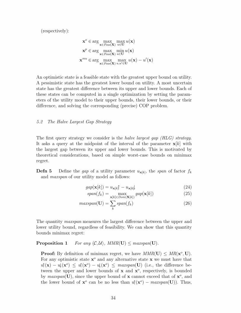
(respectively):

xo ∈ arg maxx∈Feas(X)

maxu∈U

u(x)

xp ∈ arg maxx∈Feas(X)

minu∈U

u(x)

xmu ∈ arg maxx∈Feas(X)

maxu,u′∈U

u(x) − u′(x)

An optimistic state is a feasible state with the greatest upper bound on utility.A pessimistic state has the greatest lower bound on utility. A most uncertainstate has the greatest difference between its upper and lower bounds. Each ofthese states can be computed in a single optimization by setting the param-eters of the utility model to their upper bounds, their lower bounds, or theirdifference, and solving the corresponding (precise) COP problem.

5.2 The Halve Largest Gap Strategy

The first query strategy we consider is the halve largest gap (HLG) strategy.It asks a query at the midpoint of the interval of the parameter x[k] withthe largest gap between its upper and lower bounds. This is motivated bytheoretical considerations, based on simple worst-case bounds on minimaxregret.

Defn 5 Define the gap of a utility parameter ux[k], the span of factor fk

and maxspan of our utility model as follows:

gap(x[k]) = ux[k]↑ − ux[k]↓ (24)

span(fk) = maxx[k]∈Dom(X[k])

gap(x[k]) (25)

maxspan(U) =∑k

span(fk) (26)

The quantity maxspan measures the largest difference between the upper andlower utility bound, regardless of feasibility. We can show that this quantitybounds minimax regret:

Proposition 1 For any 〈C,U〉, MMR(U) ≤ maxspan(U).

Proof: By definition of minimax regret, we have MMR(U) ≤ MR(xo,U).For any optimistic state xo and any alternative state x we must have thatu↑(x) − u↓(xo) ≤ u↑(xo) − u↓(xo) ≤ maxspan(U) (i.e., the difference be-tween the upper and lower bounds of x and xo, respectively, is boundedby maxspan(U), since the upper bound of x cannot exceed that of xo, andthe lower bound of xo can be no less than u↑(xo) − maxspan(U)). Thus,

34

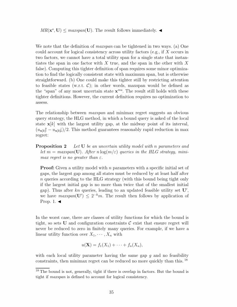
MR(xo,U) ≤ maxspan(U). The result follows immediately. J

We note that the definition of maxspan can be tightened in two ways. (a) Onecould account for logical consistency across utility factors (e.g., if X occurs intwo factors, we cannot have a total utility span for a single state that instan-tiates the span in one factor with X true, and the span in the other with Xfalse). Computing this tighter definition of span requires some minor optimiza-tion to find the logically consistent state with maximum span, but is otherwisestraightforward. (b) One could make this tighter still by restricting attentionto feasible states (w.r.t. C); in other words, maxspan would be defined asthe “span” of any most uncertain state xmu. The result still holds with thesetighter definitions. However, the current definition requires no optimization toassess.

The relationship between maxspan and minimax regret suggests an obviousquery strategy, the HLG method, in which a bound query is asked of the localstate x[k] with the largest utility gap, at the midway point of its interval,(ux[k]↑ − ux[k]↓)/2. This method guarantees reasonably rapid reduction in maxregret:

Proposition 2 Let U be an uncertain utility model with n parameters andlet m = maxspan(U). After n log(m/ε) queries in the HLG strategy, mini-max regret is no greater than ε.

Proof: Given a utility model with n parameters with a specific initial set ofgaps, the largest gap among all states must be reduced by at least half aftern queries according to the HLG strategy (with this bound being tight onlyif the largest initial gap is no more than twice that of the smallest initialgap). Thus after kn queries, leading to an updated feasible utility set U′,we have maxspan(U′) ≤ 2−km. The result then follows by application ofProp. 1. J

In the worst case, there are classes of utility functions for which the bound istight, so sets U and configuration constraints C exist that ensure regret willnever be reduced to zero in finitely many queries. For example, if we have alinear utility function over X1, · · · , Xn with

u(X) = f1(X1) + · · · + fn(Xn),

with each local utility parameter having the same gap g and no feasibilityconstraints, then minimax regret can be reduced no more quickly than this. 18

18 The bound is not, generally, tight if there is overlap in factors. But the bound istight if maxspan is defined to account for logical consistency.

35

This strategy is similar to heuristically motivated polyhedral methods in con-joint analysis used in product design and marketing [47,29]. In fact, HLG canbe viewed as a special case of the polyhedral method of [47] in which ourpolyhedra are hyper-rectangles.

5.3 The Current Solution Strategy

While HLG allows one to provide strong worst-case guarantees on regret im-provement, it is “undirected” in that considerations of feasibility play no rolein determining which queries to ask. An alternative strategy is to focus atten-tion on parameters that participate in defining minimax regret, namely, theminimax optimal x∗ and the adversarial witness xw for the current feasibleutility set U (recall that the witness xw maximizes the regret of x∗). Thecurrent solution (CS) query strategy asks about the utility parameter in theset {x∗[k] : k ≤ K} ∪ {xw[k] : k ≤ K} with largest gap(x[k]) and queries themidpoint of the corresponding utility interval. Intuitively, should the answerto a query raise the lower bound on some ux∗[k] or lower the upper bound onsome uxw[k], then the pairwise regret R(x∗,xw,U) will be reduced, and usuallyminimax regret will be reduced as well. Of course, if the answer lowers theupper bound on some ux∗[k] or raises the lower bound on some uxw[k], thenpairwise regret R(x∗,xw,U) remains unchanged and minimax regret is notguaranteed to be reduced (though it may).

We have also experimented with a variant of the CS strategy in which regretis computed approximately to ensure fast interactive response in the queryingprocess. This can be done by imposing a time bound on the solution algorithmfor computing minimax regret, exploiting the anytime nature of the methoddescribed in Sec. 4.2. While we can’t be sure we have the minimax optimalsolution with early termination, the solution may be good enough to guidethe querying process. Furthermore, since we can compute the max regret ofthe anytime solution, we have an upper bound on minimax regret which canbe used as a natural termination criterion.

5.4 Alternative Strategies

Finally, we consider several other strategies, which we describe briefly. Theoptimistic query strategy computes an optimistic state xo and queries (at themidpoint of the interval) the utility parameter in xo with the largest gap.Intuitively, an optimistic xo is a useful adversarial choice, so refining informa-tion about it can help reduce regret. The pessimistic query strategy is analo-gous, relying on the intuition that a pessimistic choice is useful in preventing

36

the adversary from making us regret our decision too much. The optimistic-pessimistic (OP) strategy combines the two intuitions: it chooses the parame-ter with largest gap among both states. These strategies are computationallyappealing since they require solving only a standard COP, not a full-fledgedminimax optimization. 19

The most uncertain state (MUS) strategy is a variant of HLG that accountsfor feasibility: we compute a most uncertain state xmu and query (at the mid-point) the parameter in xmu with the largest gap. Finally, the second-best (SB)strategy is based on the following intuition: suppose we have the optimisticstate xo and the second-best optimistic state x2o (i.e., that state with thesecond-highest upper bound—this is computable with a single optimization).If we could ask a query which reduced the upper bound utility of xo to lowerthan that of x2o, we ensure that regret is reduced (since the adversary canno longer attain this most optimistic value); if the lower bound of xo wereraised to the level of x2o’s upper bound, then we could terminate—knowingthat xo is optimal. Thus we would like to query xo at x2o’s upper bound: anegative response will reduce regret, a positive response ensures xo is optimal.Unfortunately, this cannot be implemented directly, since we can only querylocal parameters, but the strategy can be approximated for factored modelsby “distributing” this query across the different parameters and asking a setof queries.

The myopically optimal (MY) strategy computes the average regret reductionof the midpoint query for each utility parameter by solving the minimax opti-mization problem for each response to each query; it then asks the query withthe largest regret reduction averaged over both possible answers, yes and no.For large problems, this approach is computationally infeasible, but we test iton small problems to see how the other methods compare. 20

5.5 Empirical Results

To test the effectiveness of the various query strategies, we ran a series ofelicitation experiments on a variety of problems. For each problem we testedthe following elicitation strategies: halve largest gap (HLG), current solution(CS), current solution with a computation-time bound of five seconds perquery (CS-5), optimistic-pessimistic (OP), second-best (SB), and most un-certain state (MUS). In addition, on problems small enough to permit it, we

19 Even termination can be determined heuristically, for example, by computing themax regret of the optimistic state after each query, or doing minimax optimizationafter every q queries.20 By doing lookahead of k stages of this type, we could in fact compute the optimalquery plan of k-steps; however, doing so is infeasible.

37

also tested these strategies against the much more computationally demandingmyopically optimal method (MY).

We implemented the constraint generation approach outlined in Sec. 4.2 andused CPLEX 9.0 as the generic IP solver. 21 Our experiments considered tworealistic domains—car rentals and real estate—as well as randomly generatedsynthetic problems, as described in Sec. 4.3, with a factored structure sufficientto admit practical solution.

First, we experimented with a set of small synthetic problems. We did this toallow a comparison of all our proposed heuristics with the MY strategy whichis most demanding computationally. Figure 9 reports the average minimaxregret over 45 small synthetic problems constructed by randomly setting theutility bounds and the variables on which each utility factor depends. Eachproblem has ten attributes that can take at most four values and ten factorsthat depend on at most three attributes. We simulate user responses by draw-ing a random utility function u for each trial, consistent with the bounds,representing a specific user’s preferences. Responses to queries are generatedusing u, assuming that the user accurately answers all queries relative to thespecific utility function u.

Results are shown for two cases: first, for utility parameters drawn from auniform distribution over the corresponding interval; and second, for param-eters drawn from a truncated Gaussian distribution centered at the midpointof the corresponding interval and truncated at the endpoints of that interval.This second regime reflects the fact that, given some initial unquantified un-certainty about a utility parameter, a user is somewhat more likely to havea true parameter value nearer the middle of the range. However, this prob-abilistic information is used only to generate “simulated users,” and is notexploited by the elicitation algorithms. 22

In the case of both the uniform and truncated Gaussian distributions, weobserve that the OP, CS and CS-5 elicitation strategies decrease minimaxregret at a rate very close to MY. This suggests that OP, CS and CS-5 arecomputationally feasible, yet promising alternatives to the computationallyprohibitive MY strategy.

We report on further experiments using all strategies except MY (excluded forcomputational reasons) with larger synthetic problems, the real-estate problemand the car-rental problem. All results are averaged over 45 trials and use thesame regime described above, involving both uniform and truncated Gaussianpriors to generate users. Performance of the various query strategies on the

21 These simulations were performed on 3.0 GHz PCs.22 All experiments show a reasonably small variance so we exclude error bars forlegibility.

38

0 50 100 150 2000

20

40

60

80

100

120

140

Number of queries

Min

imax

reg

ret

Small Random Problem −− Uniform Prior

0%

3%

6%

9%

12%

15%

17%

20%

Min

imax

reg

ret /

max

util

ity

CS−5

CS

HLG

MUSMY

SB

OP

0 50 100 150 2000

20

40

60

80

100

120

140

Number of queries

Min

imax

reg

ret

Small Random Problem −− Gaussian Prior

0%

3%

6%

9%

12%

15%

17%

20%

Min

imax

reg

ret /

max

util

ity

CS−5

CS

HLG

MUS

MY

SB

OP

Fig. 9. Average max regret on small random problems (45 instances) as a functionof number of queries given (a) uniform and (b) Gaussian distributed utilities.

0 50 100 150 2000

50

100

150

200

250

300

350

399

Number of queries

Min

imax

reg

ret

Car Rental Problem −− Uniform Prior

0%

2%

4%

7%

9%

11%

13%

16%

18%

Min

imax

reg

ret /

max

util

ity

CS−5

CSHLG

MUS

SB

OP

0 50 100 150 2000

100

200

300

399

Number of queries

Min

imax

reg

ret

Car Rental Problem −− Gaussian Prior

0%

4%

9%

13%

18%

Min

imax

reg

ret /

max

util

ity

CS−5CS

HLG

MUS

SB

OP

Fig. 10. Average max regret on car-rental problem (45 instances) as a function ofnumber of queries given (a) uniform and (b) Gaussian distributed utilities.

car rental problem is depicted in Figure 10, showing average minimax regretas a function of the number of queries. Initial utility bounds are set to giveminimax regret of roughly 18% of the optimal solution.

Both CS and CS-5 perform extremely well: regret is reduced to almost zerowithin 160 queries on average. Though this may seem like a lot of queries,recall that the problem is itself large and the utility model has 150 parame-ters. We intentionally choose problems this large to push the computationalboundaries of regret-based elicitation. Furthermore, while 160 queries may belarge for typical consumer choice problems, it is more than reasonable for highstakes configuration applications. More importantly, these methods show ex-cellent anytime performance: after only 80 queries, average minimax regrethas dropped from 18% to under 2%.

Interestingly, the time bound of five seconds imposed by CS-5, while leadingto approximately minimax optimal solutions, does not affect query quality:the approximate solutions give rise to queries that are virtually as effective as

39

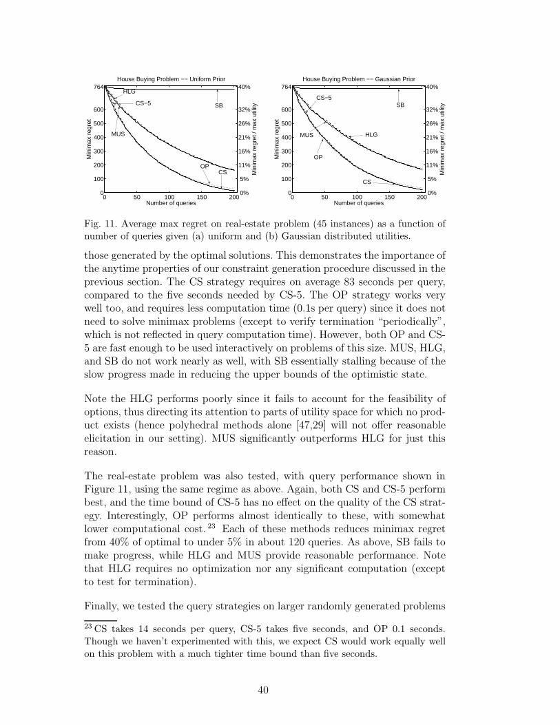
0 50 100 150 2000

100

200

300

400

500

600

764

Number of queries

Min

imax

reg

ret

House Buying Problem −− Uniform Prior

0%

5%

11%

16%

21%

26%

32%

40%

Min

imax

reg

ret /

max

util

ity

CS−5

CS

HLG

MUS

SB

OP

0 50 100 150 2000

100

200

300

400

500

600

764

Number of queries

Min

imax

reg

ret

House Buying Problem −− Gaussian Prior

0%

5%

11%

16%

21%

26%

32%

40%

Min

imax

reg

ret /

max

util

ity

CS−5

CS

HLGMUS

SB

OP

Fig. 11. Average max regret on real-estate problem (45 instances) as a function ofnumber of queries given (a) uniform and (b) Gaussian distributed utilities.

those generated by the optimal solutions. This demonstrates the importance ofthe anytime properties of our constraint generation procedure discussed in theprevious section. The CS strategy requires on average 83 seconds per query,compared to the five seconds needed by CS-5. The OP strategy works verywell too, and requires less computation time (0.1s per query) since it does notneed to solve minimax problems (except to verify termination “periodically”,which is not reflected in query computation time). However, both OP and CS-5 are fast enough to be used interactively on problems of this size. MUS, HLG,and SB do not work nearly as well, with SB essentially stalling because of theslow progress made in reducing the upper bounds of the optimistic state.

Note the HLG performs poorly since it fails to account for the feasibility ofoptions, thus directing its attention to parts of utility space for which no prod-uct exists (hence polyhedral methods alone [47,29] will not offer reasonableelicitation in our setting). MUS significantly outperforms HLG for just thisreason.

The real-estate problem was also tested, with query performance shown inFigure 11, using the same regime as above. Again, both CS and CS-5 performbest, and the time bound of CS-5 has no effect on the quality of the CS strat-egy. Interestingly, OP performs almost identically to these, with somewhatlower computational cost. 23 Each of these methods reduces minimax regretfrom 40% of optimal to under 5% in about 120 queries. As above, SB fails tomake progress, while HLG and MUS provide reasonable performance. Notethat HLG requires no optimization nor any significant computation (exceptto test for termination).

Finally, we tested the query strategies on larger randomly generated problems

23 CS takes 14 seconds per query, CS-5 takes five seconds, and OP 0.1 seconds.Though we haven’t experimented with this, we expect CS would work equally wellon this problem with a much tighter time bound than five seconds.

40

0 50 100 150 2000

50

100

150

200

250

300

350

400

450

512

Number of queries

Min

imax

reg

ret

Large Random Problem −− Uniform Prior

0%

4%

7%

11%

14%

18%

21%

25%

28%

32%

36%

Min

imax

reg

ret /

max

util

ity

CS−5

CS

HLG

MUS

SB

OP

0 50 100 150 2000

50

100

150

200

250

300

350

400

450

512

Number of queries

Min

imax

reg

ret

Large Random Problem −− Gaussian Prior

0%

3%

7%

10%

14%

17%

21%

24%

28%

31%

35%

Min

imax

reg

ret /

max

util

ity

CS−5

CS

HLG

MUS

SB

OP

Fig. 12. Average max regret on large random problems (45 instances) as a functionof number of queries given (a) uniform and (b) Gaussian distributed utilities.

(with 25 variables of domain size no more than four, and 20 utility factorswith no more than three variables each). Results are shown in Figure 12. Thesame performance patterns as in the real-estate problem emerge, with CS, CS-5 and OP all performing much better than the others. Although OP performsslightly better than CS/CS-5, the difference is not statistically significant.

5.6 Comparison Queries

Comparison queries provide a natural alternative to bound queries in manysituations. A comparison query takes the form “Do you prefer x to x′?” Apositive response implies that ux > ux′. If the utility model is factored, thiscorresponds to the following linear constraint:

∑k

ux[k] >∑k

ux′[k].

A negative response imposes the complementary constraint.

Given a collection of linear constraints U imposed by responses to a sequenceof comparison queries, the minimax optimal decision can be computed usingthe constraint generation procedure described in Sec. 4.4. Our generic elic-itation algorithm can then be used to ask specific comparison queries untilminimax regret reaches an acceptable level. Though we do not experimentwith specific comparison query strategies here, we expect that a modificationof the current solution (CS) strategy proposed for bound queries would workespecially well with comparison queries. More precisely, suppose that given thecurrent constraints U , the minimax optimal solution is computed to be x∗ withadversarial witness xw. The CS query strategy for comparison queries requiresthat we ask the user to compare x∗ and xw. Should the user prefer x∗, thisrules out the adversary’s chosen utility function from the feasible set U, thus

41

ensuring a reduction in the pairwise regret R(x∗,xw,U) to zero, and usuallyreducing minimax regret as well. If xw is preferred, this does not rule out theadversary’s chosen utility function, nor is it guaranteed to reduce regret, butgenerally imposes a fairly strong constraint on U. Given the success of thisstrategy with respect to bound queries, and the success of related strategiesin other domains [13,14], we expect the CS strategy to perform quite well.

Unlike the case of bound queries, where it is quite clear (due to the focuson gaps in specific parameters) that a user cannot provide a response that isinconsistent with prior responses, it is not obvious that a user cannot be in-consistent in responding to comparison queries. However, the CS strategy forbound queries does indeed ensure consistency. Unless minimax regret is zero(in which case the process would terminate), there must be some utility func-tion in the current feasible set U for which xw is preferred to x∗. Furthermore,there must be some utility function for which x∗ is preferred to xw; otherwise,xw would have regret no greater that that of x∗ under all u ∈ U , and wouldthus be minimax optimal as well (also implying that, since it is the witness,that minimax regret is zero).

6 Concluding Remarks

Preference elicitation techniques for constraint-based optimization problemsare critical to the development of interactive decision software. We have begunto address several important issues in this regard, specifically, how one shouldmake decisions in the presence of (non-probabilistic) utility function uncer-tainty, and elicitation strategies that improve decision quality with minimalinteraction. We have developed techniques for computing minimax optimaldecisions in constraint-based decision problems when a user’s utility functionis only partially specified in the form of upper and lower bounds on utility pa-rameters, or arbitrary linear constraints on such parameters. While the corre-sponding optimizations are potentially complex, we derived methods wherebythey could be solved effectively using a sequence of MIPs. Furthermore, weshowed how structure in the utility model could be exploited to ensure thatthe resulting IPs are compact or could be solved using an effective constraintgeneration procedure. Experiments with utility uncertainty specified by pa-rameter bounds demonstrated the practicality of these techniques.

We also developed a number of query strategies for eliciting bounds on theparameters of utility models for the purpose of solving imprecise COPs. Themost promising of these strategies, CS and OP, perform extremely well, requir-ing very few queries (relative to the model size) to provide dramatic reductionsin regret. We have shown that using approximation of minimax regret reducesinteractive computation time to levels required for real-time response with-

42

out a noticeable effect on the performance of CS. OP also can be executed inreal-time, since it does not require the same intensive minimax computation.

There are a number of directions in which this work can be extended. Forexample, the use of search and constraint-propagation methods for solvingthe COPs associated with computing minimax regret is of great interest. Ourgoal in this paper was to provide a precise formulation of these computationalproblems as integer programs, and use off-the-shelf software to solve them. Weexpect that constraint-based optimization techniques that are specifically di-rected toward these problems should prove fruitful. Along these lines, we hopeto develop deeper connections to existing work on soft constraints, valued-CSPs, and related frameworks.

Experimental validation of our suggested approach for comparison queries isan important next step, as is the development of new query strategies. Inpractice, we can often assume or develop prior distributional information overutilities. Rather than asking queries at midpoints of intervals, we could opti-mize the query point using probabilistic (value of information) computation,while using (distribution-free) regret to make decisions [49]. We are quite in-terested in the possibility of integrating Bayesian methods for reasoning aboutuncertain utility functions [17,10,27] with the constraint-based representationof the decision space. Finally, while optimal (non-myopic) strategies could befound (in principle) by solving prohibitively large continuous MDPs, it wouldnevertheless be interesting to explore non-myopic heuristics, and investigatethe extent to which lookahead information can improve the reduction in min-imax regret.

Naturally, we would like to consider additional query types, as well as alter-native means for structuring outcomes and interactions to ease the cognitiveburden on users. Developing means to improve robustness of our methods tothe types of errors users typically make is also critical if tools such as those pro-posed here are to find widespread use. As such, user studies with our modelswill be required in order to assess the naturalness of such interaction modelsand to further refine our techniques to make them more understandable andintuitive for users.

An important question left unaddressed is that of eliciting the structure ofa GAI model. Our work here assumes that the GAI factorization has beengiven and elicits only parameters of this model. We are currently exploringthe application of techniques from decision analysis and elicitation of graphicalmodels to the automated elicitation of GAI model structure.

43

Acknowledgements

This research was supported by the the Institute for Robotics and IntelligentSystems (IRIS) and the Natural Sciences and Engineering Research Council(NSERC). Poupart was supported by a scholarship provided by Precarn In-corporated through IRIS. Thanks to the anonymous referees for their helpfulsuggestions.

References

[1] Igor Averbakh. Minmax regret solutions for minimax optimization problemswith uncertainty. Operations Research Letters, 27:57–65, 2000.

[2] Igor Averbakh and Vasilij Lebedev. On the complexity of minmax regret linearprogramming. European Journal of Operational Research, 160(1):227–231, 2005.

[3] Fahiem Bacchus and Adam Grove. Graphical models for preference andutility. In Proceedings of the Eleventh Conference on Uncertainty in ArtificialIntelligence, pages 3–10, Montreal, 1995.

[4] David E. Bell. Regret in decision making under uncertainty. OperationsResearch, 30:961–981, 1982.

[5] Aharon Ben-Tal and Arkadi Nemirovski. Robust solutions of uncertain linearprograms. Operations Research Letters, 25:1–13, 1999.

[6] J. F. Benders. Partitioning procedures for solving mixed-variables programmingproblems. Numerische Mathematik, 4:238–252, 1962.

[7] Umberto Bertele and Francesco Brioschi. Nonserial Dynamic Programming.Academic Press, Orlando, 1972.

[8] Stefano Bistarelli, Ugo Montanari, and Francesca Rossi. Semiring-basedconstraint satisfaction and optimization. Journal of the ACM, 44(2):201–236,1997.

[9] Jim Blythe. Visual exploration and incremental utility elicitation. InProceedings of the Eighteenth National Conference on Artificial Intelligence,pages 526–532, Edmonton, 2002.

[10] Craig Boutilier. A POMDP formulation of preference elicitation problems. InProceedings of the Eighteenth National Conference on Artificial Intelligence,pages 239–246, Edmonton, 2002.

[11] Craig Boutilier. On the foundations of expected expected utility. In Proceedingsof the Eighteenth International Joint Conference on Artificial Intelligence, pages285–290, Acapulco, 2003.

44

[12] Craig Boutilier, Fahiem Bacchus, and Ronen I. Brafman. UCP-Networks: Adirected graphical representation of conditional utilities. In Proceedings of theSeventeenth Conference on Uncertainty in Artificial Intelligence, pages 56–64,Seattle, 2001.

[13] Craig Boutilier, Rajarshi Das, Jeffrey O. Kephart, Gerald Tesauro, andWilliam E. Walsh. Cooperative negotiation in autonomic systems usingincremental utility elicitation. In Proceedings of the Nineteenth Conference onUncertainty in Artificial Intelligence, pages 89–97, Acapulco, 2003.

[14] Craig Boutilier, Tuomas Sandholm, and Rob Shields. Eliciting bid taker non-price preferences in (combinatorial) auctions. In Proceedings of the NineteenthNational Conference on Artificial Intelligence, pages 204–211, San Jose, CA,2004.

[15] Darius Braziunas and Craig Boutilier. Local utility elicitation in GAI models.In Proceedings of the Twenty-first Conference on Uncertainty in ArtificialIntelligence, pages 42–49, Edinburgh, 2005.

[16] Urszula Chajewska, Lise Getoor, Joseph Norman, and Yuval Shahar. Utilityelicitation as a classification problem. In Proceedings of the FourteenthConference on Uncertainty in Artificial Intelligence, pages 79–88, Madison, WI,1998.

[17] Urszula Chajewska, Daphne Koller, and Ronald Parr. Making rational decisionsusing adaptive utility elicitation. In Proceedings of the Seventeenth NationalConference on Artificial Intelligence, pages 363–369, Austin, TX, 2000.

[18] Vijay Chandru and John N. Hooker. Optimization Methods for LogicalInference. Wiley, New York, 1999.

[19] Rina Dechter. Bucket elimination: A unifying framework for probabilisticinference. In Proceedings of the Twelfth Conference on Uncertainty in ArtificialIntelligence, pages 211–219, Portland, OR, 1996.

[20] Rina Dechter. Constraint Processing. Morgan Kaufmann, San Francisco, 2003.

[21] James S. Dyer. Interactive goal programming. Management Science, 19:62–70,1972.

[22] Peter C. Fishburn. Interdependence and additivity in multivariate,unidimensional expected utility theory. International Economic Review, 8:335–342, 1967.

[23] Peter C. Fishburn. Utility Theory for Decision Making. Wiley, New York, 1970.

[24] Simon French. Decision Theory. Halsted Press, New York, 1986.

[25] Christophe Gonzales and Patrice Perny. GAI networks for utility elicitation. InProceedings of the Ninth International Conference on Principles of KnowledgeRepresentation and Reasoning (KR2004), pages 224–234, Whistler, BC, 2004.

45

[26] Carlos Guestrin, Daphne Koller, and Ronald Parr. Max-norm projectionsfor factored MDPs. In Proceedings of the Seventeenth International JointConference on Artificial Intelligence, pages 673–680, Seattle, 2001.

[27] Hillary A. Holloway and Chelsea C. White, III. Question selection formultiattribute decision-aiding. European Journal of Operational Research,148:525–543, 2003.

[28] Eric Horvitz, Jack Breese, David Heckerman, David Hovel, and Koos Rommelse.The lumiere project: Bayesian user modeling for inferring goals and needs ofsoftware users. In Proceedings of the Fourteenth Conference on Uncertainty inArtificial Intelligence, pages 256–265, Madison, WI, 1998.

[29] Vijay S. Iyengar, Jon Lee, and Murray Campbell. Q-Eval: Evaluating multipleattribute items using queries. In Proceedings of the Third ACM Conference onElectronic Commerce, pages 144–153, Tampa, FL, 2001.

[30] Ralph L. Keeney and Howard Raiffa. Decisions with Multiple Objectives:Preferences and Value Trade-offs. Wiley, New York, 1976.

[31] Joseph A. Konstan, Bradley N. Miller, David Maltz, Jonathan L. Herlocker,Lee R. Gordon, and John Riedl. Grouplens: Applying collaborative filtering tousenet news. Communications of the ACM, 40(3):77–87, 1997.

[32] Panos Kouvelis and Gang Yu. Robust Discrete Optimization and ItsApplications. Kluwer, Dordrecht, 1997.

[33] G. Lee, S. Bauer, P. Faratin, and J. Wroclawski. Learning user preferencesfor wireless services provisioning. In Proceedings of the Third InternationalJoint Conference on Autonomous Agents and Multiagent Systems (AAMAS-04), pages 480–487, New York, 2004.

[34] Graham Loomes and Robert Sugden. Regret theory: An alternative theory ofrational choice under uncertainty. Economic Journal, 92:805–824, 1982.

[35] Amparo M. Marmol, Justo Puerto, and Francisco R. Fernandez. The use ofpartial information on weights in multicriteria decision problems. Journal ofMulticriteria Decision Analysis, 7:322–329, 1998.

[36] George L. Nemhauser and Laurence A. Wolsey. Integer Programming andCombinatorial Optimization. Wiley, New York, 1988.

[37] Barry O’Sullivan, Eugene Freuder, and Sarah O’Connell. Interactive constraintacquisition. In CP-2001 Workshop on User Interaction in ConstraintProcessing, Paphos, Cyprus, 2001.

[38] Pearl Pu, Boi Faltings, and Marc Torrens. User-involved preference elicitation.In IJCAI-03 Workshop on Configuration, Acapulco, 2003.

[39] John C. Quiggan. Stochastic dominance in regret theory. The Review ofEconomic Studies, 57(3):503–511, 1990.

46

[40] Francesca Rossi, Alessandro Sperduti, Kristen Brent Venable, Lina Khatib,Paul H. Morris, and Robert A. Morris. Learning and solving soft temporalconstraints: An experimental study. In Proceedings of the Eighth InternationalConference on Principles and Practice of Constraint Programming, pages 249–263, Ithaca, NY, 2002.

[41] Daniel Sabin and Rainer Weigel. Product configuration frameworks—a survey.IEEE Intelligent Systems and their Applications, 13(4):42–49, 1998.

[42] Ahti Salo and Raimo P. Hamalainen. Preference ratios in multiattributeevaluation (PRIME)–elicitation and decision procedures under incompleteinformation. IEEE Trans. on Systems, Man and Cybernetics, 31(6):533–545,2001.

[43] Leonard J. Savage. The Foundations of Statistics. Wiley, New York, 1954.

[44] Leonard J. Savage. The theory of statistical decision. Journal of the AmericanStatistical Association, 46:55–67, 1986.

[45] Thomas Schiex, Helene Fargier, and Gerard Verfaillie. Valued constraintsatisfaction problems: Hard and easy problems. In Proceedings of theFourteenth International Joint Conference on Artificial Intelligence, pages 631–637, Montreal, 1995.

[46] Dale Schuurmans and Relu Patrascu. Direct value approximation for factoredMDPs. In Advances in Neural Information Processing Systems 14 (NIPS-2001),pages 1579–1586, Vancouver, 2001.

[47] Olivier Toubia, John Hauser, and Duncan Simester. Polyhedral methods foradaptive choice-based conjoint analysis. Technical Report 4285-03, Sloan Schoolof Management, MIT, Cambridge, 2003.

[48] John von Neumann and Oskar Morgenstern. Theory of Games and EconomicBehavior. Princeton University Press, Princeton, 1944.

[49] Tianhan Wang and Craig Boutilier. Incremental utility elicitation with theminimax regret decision criterion. In Proceedings of the Eighteenth InternationalJoint Conference on Artificial Intelligence, pages 309–316, Acapulco, 2003.

[50] Martin Weber. Decision making with incomplete information. European Journalof Operational Research, 28:44–57, 1987.

[51] Chelsea C. White, III, Andrew P. Sage, and Shigeru Dozono. A modelof multiattribute decisionmaking and trade-off weight determination underuncertainty. IEEE Transactions on Systems, Man and Cybernetics, 14(2):223–229, 1984.

47