constrained-based differential privacy for mobility...
TRANSCRIPT
Constrained-Based Differential Privacy for Mobility ServicesFerdinando Fioretto
University of Michigan
Ann Arbor, MI, USA
Chansoo Lee
University of Michigan
Ann Arbor, MI, USA
Pascal Van Hentenryck
University of Michigan
Ann Arbor, MI, USA
ABSTRACTUbiquitous mobile and wireless communication systems have the
potential to revolutionize transportation systems, making accurate
mobility traces and activity-based patterns available to optimize
the design and operations of mobility systems. However, these rich
data sets also pose significant privacy risks, potentially revealing
highly sensitive information about individual agents.
This paper studies how to use differential privacy to release mo-
bility data for transportation applications. It shows that existing
approaches do not provide the desired fidelity for practical uses. To
remedy this limitation, the paper proposes the idea of Constraint-Based Differential Privacy (CBDP) that casts the production of a
private data set as an optimization problem that redistributes the
noise introduced by a randomized mechanism to satisfy fundamen-
tal constraints of the original data set.
The CBDP has strong theoretical guarantees: It is a constant
factor away from optimality and when the constraints capture
categorical features, it runs in polynomial time. Experimental re-
sults show that CBDP ensures that a city-level multi-modal transit
system has similar performance measures when designed and opti-
mized over the real and private data sets and improves state-of-art
privacy methods by an order of magnitude.
KEYWORDSDifferential Privacy; Mobility; Transportation;
ACM Reference Format:Ferdinando Fioretto, Chansoo Lee, and Pascal Van Hentenryck. 2018. Con-
strained-Based Differential Privacy for Mobility Services. In Proc. of the17th International Conference on Autonomous Agents and Multiagent Systems(AAMAS 2018), Stockholm, Sweden, July 10–15, 2018, IFAAMAS, 9 pages.
1 INTRODUCTIONThe availability of mobility traces and activity-based patterns has
the potential to revolutionize the design and operations of trans-
portation systems. For instance, shared-ride services such as Uber-Pool and Via reroute driver paths in real time to optimize vehicle
capacity, bike-sharing programs such as CitiBike in New York re-
balance their fleets from popular destinations to popular origins,
and CityMapper operates a private night bus line in London based
on their analysis of the mobility data collected from user data.
However, the release of mobility data poses significant risks, as
they contain highly sensitive information about individual agents,
Proc. of the 17th International Conference on Autonomous Agents and Multiagent Systems(AAMAS 2018), M. Dastani, G. Sukthankar, E. André, S. Koenig (eds.), July 10–15, 2018,Stockholm, Sweden. © 2018 International Foundation for Autonomous Agents and
Multiagent Systems (www.ifaamas.org). All rights reserved.
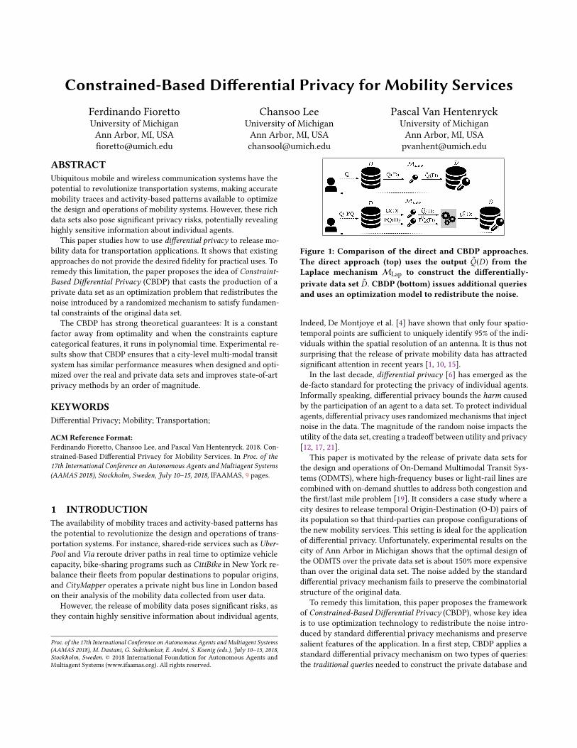
Figure 1: Comparison of the direct and CBDP approaches.The direct approach (top) uses the output Q̃(D) from theLaplace mechanism MLap to construct the differentially-private data set D̃. CBDP (bottom) issues additional queriesand uses an optimization model to redistribute the noise.
Indeed, De Montjoye et al. [4] have shown that only four spatio-
temporal points are sufficient to uniquely identify 95% of the indi-
viduals within the spatial resolution of an antenna. It is thus not
surprising that the release of private mobility data has attracted
significant attention in recent years [1, 10, 15].
In the last decade, differential privacy [6] has emerged as the
de-facto standard for protecting the privacy of individual agents.
Informally speaking, differential privacy bounds the harm caused
by the participation of an agent to a data set. To protect individual
agents, differential privacy uses randomized mechanisms that inject
noise in the data. The magnitude of the random noise impacts the
utility of the data set, creating a tradeoff between utility and privacy
[12, 17, 21].
This paper is motivated by the release of private data sets for
the design and operations of On-Demand Multimodal Transit Sys-
tems (ODMTS), where high-frequency buses or light-rail lines are
combined with on-demand shuttles to address both congestion and
the first/last mile problem [19]. It considers a case study where a
city desires to release temporal Origin-Destination (O-D) pairs of
its population so that third-parties can propose configurations of
the new mobility services. This setting is ideal for the application
of differential privacy. Unfortunately, experimental results on the
city of Ann Arbor in Michigan shows that the optimal design of
the ODMTS over the private data set is about 150% more expensive
than over the original data set. The noise added by the standard
differential privacy mechanism fails to preserve the combinatorial
structure of the original data.
To remedy this limitation, this paper proposes the framework
of Constrained-Based Differential Privacy (CBDP), whose key idea
is to use optimization technology to redistribute the noise intro-
duced by standard differential privacy mechanisms and preserve
salient features of the application. In a first step, CBDP applies a
standard differential privacy mechanism on two types of queries:
the traditional queries needed to construct the private database and

a collection of feature queries that capture important constraintsof the targeted application. Since differential privacy mechanisms
introduce noise independently on each query, the resulting query
outputs, and the private data set, are inconsistent. The second step
of CBDP uses an optimization model to redistribute the noise in
order to restore consistency and ensure that the noise stays as close
as possible to the one in the standard mechanism. Figure 1 high-
lights the difference between the direct (top row) and the CBDP
(bottom row) approaches.
The paper shows that the CBDP has strong theoretical properties:
it achieves ϵ-differential privacy, it ensures query consistency, and
it is a constant factor away from optimality. When the constraints
capture categorical features, the CBDP mechanism also runs in
polynomial time. Finally, experimental results shows that the CBDP
mechanism is also practical: On the design of an ODMTS for the
city of Ann Arbor, MI, it improves the accuracy existing approaches
by an order of magnitude and results in negligible utility losses.
2 DIFFERENTIAL PRIVACYThis section summarizes key results in Differential Privacy (DP)
[8]. A randomized mechanism M : D → R with domain D and
range R is ϵ-differentially private if, for any S ⊆ R and any two
inputs D1,D2 ∈ D differing in at most one data item1(written
| |D1 − D2 | |1 ≤ 1),
Pr [M(D1) ∈ S] ≤ exp(ϵ)Pr [M(D2) ∈ S], (1)
where the probability is calculated over the coin tosses of M. The
parameter ϵ is the privacy budget of the mechanism.
Differential privacy satisfies several important properties, includ-
ing composability and immunity to post-processing. Composability
ensures that a combination of differentially private mechanisms
preserves differential privacy.
Theorem 2.1 (Composition Theorem). LetMi : D → Ri be anϵi -differentially private mechanism (1 ≤ i ≤ k). Their compositionM(D) = (Mi (D), . . . ,Mk (D)) is (
∑ki=1 ϵi )-differentially private.
The immunity to post-processing ensures that applying arbitrarily
many functions to the output of a differentially private-mechanism
preserves its privacy guarantees.
Theorem 2.2 (Post-Processing Immunity). Let M : D → Rbe an ϵ-differentially private mechanism and д : R → R ′ be an(arbitrary) mapping. The mechanism д ◦M is ϵ-differentially private.
In private data analysis settings, agents interact with the data set
by issuing queries. A (numeric) query is a function from a data set
D ∈ D to a result set R ⊆ Rn . The sensitivity of a queryQ , denoted
by ∆Q , is defined as
∆Q = max
D1,D2 s.t.
| |D1−D2 | |1≤1
| |Q(D1) −Q(D2)| |1. (2)
Counting queries are particularly useful and return the number of
data points satisfying a predicate. They have sensitivity 1.
Adding Laplacian noise when answering numeric queries pro-
duces a differentially private mechanism [6].
1I.e., |(D1 − D2) ∪ (D2 − D1) | = 1
Figure 2: A Multimodal Transit System. Squares denoteboarding/alighting stops. Colors highlight different servicezones. The line segment illustrates amulti-modal three-legsroute (shuttle-bus-shuttle).
Theorem 2.3 (Laplace Mechanism). Let Q : D → R be a nu-merical query. The Laplace mechanism, defined asMLap(D;Q, ϵ) =Q(D) + z where z ∈ R is a vector of i.i.d. samples drawn from theLaplace distribution with scaling factor ∆f /ϵ , is ϵ-differential private.
3 ON-DEMAND MULTIMODAL TRANSITOn-Demand multimodal transit systems (ODMTS) jointly address
congestion and the first/last mile problem that plagues many transit
systems. They combine high-frequency buses (or light-rail) between
hubs for high-density corridors, with on-demand shuttles to bring
riders from their origins to the hubs and from the hubs to their
destinations. On-demand shuttles also perform direct trips between
origins and destinations. Bus routes are fixed, while the shuttles are
dispatched and routed dynamically, maximizing ride sharing while
preserving short waiting and transit times for passengers. Riders
are picked up and dropped off at virtual vehicle stops (also called
locations for simplicity), which include the hubs. Figure 2 illustrates
a trip with three legs in an ODMTS consisting a shuttle leg from
the trip origin (location ℓ1) to a hub (location ℓ2), followed by a bus
leg to another hub (location ℓ3) and a final shuttle leg to the final
destination (location ℓ4).
The design of an ODMTS aims at minimizing the total cost of the
system (investment and operating costs), while keeping the average
transit time within a desired interval. Maheo et al. [19] proposed an
advanced Benders decomposition algorithm to design an optimal
ODMTS from a data set of temporal O-D pairs. When scaling to
large cities or significant riderships, it is also desirable to partition
the transit region into zones, which are operated and optimized
independently. In particular, each zone are allocated a number of
shuttles that serve the requests within the zone and from the zone
to a hub (and vice-versa). In Figure 2, the zones are depicted by the
color of the stops. The design of an ODMTS must then optimally
size the fleet of each zone and determine a cost-optimal rostering of
the drivers that obeys federal and state regulations. Finally, during
operations, real-time algorithms for shuttle dispatching, routing,
and ride-sharing aim at minimizing the average transit times of
riders, while satisfying convenience constraints.
For concreteness, the paper focuses on the following case study.
A transit agency has designed an ODMTS, including the bus net-
work and the shuttle zones, and would like to engage a mobility

solution provider for servicing the shuttle component. To help the
procurement process, the transit agency would like to release a pri-
vate data set so that mobility solution providers can size their fleets
properly to minimize cost and satisfy the selected performance
criteria for waiting and transit times. Mobile solution providers
will then use their optimization algorithms for fleet sizing and real-
time operations, denoted by F and O respectively, in order to price
their services accurately. This case study is representative of many
procurement and competition settings.
4 NOTATIONS AND SETTINGSLet N0 be the set of non-negative integers and U the data universe,which we assume to be a finite set. A data set D is a multi-set of
elements in U or, equivalently, a vector inN|U |
0. The data universe
for our mobility data set is defined asU = L×L×T, where L is a set
of locations (virtual vehicle stops) and T is a partition of a 24-hour
day in time periods. The time resolution determines the cardinality
of T. Elements in U are called trip types and are denoted by ⟨o,d, t⟩,where o,d ∈ L are the origin and destination of the request and
t ∈ T represents its time period. Our mobility data set is a multiset
of trip types or, equivalently, a vector of type N|L2T |0
.
This paper studies the release of a private version of a data
set, which is then used in a procurement or competition context.
The original data set can be obtained by numeric queries on every
u ∈ U . Similarly, a private data set can be produced via a mapping
from noisy outputs c̃u to these numeric queries. As a result, this
paper primarily focuses on differential-privacy mechanisms for
these numeric queries.
5 RELATEDWORKAs sketched in the introduction, the first step of CBDP uses a se-
quence of correlated (batched) queries. Research on answering
batched queries has focused primarily at reducing the sensitivity of
correlated queries. Xiao et al. [24] applies a wavelet transformation
to the data set frequency to generate a wavelet coefficient resulting
in reduced noise variance per query. Li et al. [16] proposed amatrixmechanism to answer linear combinations of queries. Huang et
al. [13] applies a transformation to the batch of queries to output a
set of orthogonal queries to reduce correlation between them. The
literature on k-way marginals [5, 7, 22] focuses on improving the
time complexity or accuracy when the data universe is so large that
the full marginal is unnecessary and infeasible. In contrast, CBDPreleases the full private data set, imposes constraints to ensure itsconsistency, and optimization to guarantee its accuracy.
The closest related work is the Hierarchical (H) mechanism of
Hay et al. [11] and its extensions [2, 21]. It uses a post-processing
step that enforces additive constraints based on a tree structure of
the data universe. The mechanism creates a balanced tree where
the leaves are singleton sets of the universe U , each internal node
is the union of its children, and the root is the entire universe. For a
tree of height h, H first uses the Laplace mechanism for answering a
counting query for each node of the tree (except the root). Each such
query has a privacy parameter ϵ/h, so that the step is ϵ-differentially
private. The second step of H takes the resulting tree T0 ∈ R |U |
and applies a variance reduction process to obtain a tree T1. Thefinal step in H finds a tree T in which a parent value is equal to the
sum of values of its children and the value ∥T −T1∥2
2is minimized.
Thanks to the tree structure and simplicity of the objective, there is
a simple closed form formula to computeT . The leaves can then be
used to reconstruct a data set. Although the original hierarchical
mechanism only considers balanced trees and is agnostic to the
data semantics, it can be altered to use features for branching and
is thus directly applicable to the setting of this paper. A detailed
comparison of CBDP and H is presented in Section 11.
6 THE DIFFERENTIAL PRIVACY CHALLENGEIt is useful to highlight the challenges raised by the case study. For
the OBMTS of Ann Arbor, the Laplace mechanism on the batched
queries outputs a real vector with many negative numbers (which
are obviously semantically meaningless). A post-processing step
that rounds each count to its closest non-negative number induces
a significant bias towards positive noise values. This problem is
exacerbated by the sparsity of our query results. For the considered
OBMTS, the original data set contains 37,714 trips. The Laplace
mechanism for ϵ = 1 returns on average of 261,032 trips (averaged
over 50 independent runs), which is about a 7 fold increase. For
ϵ = 0.01, the Laplace mechanism generates 3,312,350 trips just
between 8am-10am compared to 4878 actual trips. As a result, a
fleet-sizing optimizer will significantly overestimate the number
of shuttles required and the overall operating cost of the ODMTS,
making the release of the private data set useless.
To understand these results, it is useful to observe that, for a
resolution of 30 minutes, there are 67600 possible trip types within
the two-hour period 8am–10am. However, only 591 of them have
non-zero counts. This pathological behavior of the Laplace mech-
anism on sparse counting queries is a well-known critical issue
when applying differential privacy in practice [3, 9, 18, 23].
7 THE CBDP MECHANISMTo remedy this important issue, this paper introduces the idea
of Constraint-Based Differential Privacy (CBDP). It is especially
suitable for complex optimization tasks whose outcomes, crucially,
but indirectly, depend on structural properties of the data. CBDP
uses the concept of features to capture semantic properties of the
application and queries these features in addition to the orginal
data set.
Features and Feature Queries. A central element of CBDP is the
concept of feature. A (categorical) feature is a partition of the uni-
verse U and the size of the feature is the number of elements in
the partition. A feature F′ is a sub-feature of F, denoted by F′ ≺ F,if F′ is obtained by sub-partitioning F. The feature query on data
set D ∈ D associated with feature F = {d1, . . . , dn } is denoted by
QF(D): It returns an n-dimensional count vector (c1, . . . , cn ) whereeach ci is the number of data points in D that belong to di .
The Input. The mechanisms studied in this paper take as input
the data set D and a collection of features F = {F1, . . . , Fk } whereFi = {di1, . . . , dini } for (i = 1, . . . ,k). For simplicity, the first feature
always partitions the universe into singletons, i.e., F1 = {{u} : u ∈
U }, since these are the counts used to construct the private data
set. The paper also assumes that the second feature contains the
universe as a single element, i.e., F2 = {U }. Hence, query QF1 (D)

minimize: ∥x − c̃∥22,w =
k∑i=1
1
ni
ni∑j=1
(xi j − c̃i j )2 (O1)
subject to:
∀i′, i : Fi′ ≺ Fi , j ∈ [ni ] : xi j =∑
l :di′l ⊆di j
xi′l (O2)
∀i, j : xi j ≥ 0. (O3)
Figure 3: The CBDP Post-Processing Step.
reports the counts of the original data set D, while query QF2 (D)reports the total number of elements in the data set.When viewed as
queries, the inputs to the mechanism can be represented as a set of
counts QFi = ci = (ci1, . . . , cini ) (1 ≤ i ≤ k) or, more concisely, as
c = (c11, . . . , cknk ). Finally, for simplicity, the mechanisms assume
that the partial ordering ≺ of features is given.
The CBDPMechanism. CBDPfirst applies the Laplacemechanism
with privacy parameterϵk to each feature query, i.e.,
MLap(D;QFi , ϵ/k) = c̃i = (c̃i1, . . . , c̃ini ) ∈ Rni (1 ≤ i ≤ k).
The resulting counts c̃ = (c̃11, . . . , c̃knk ) are then post-processed
by the optimization algorithm depicted in Figure 3 to obtain the
counts x∗ = (x∗11. . . ,x∗knk
). Finally, the CBDP mechanism outputs
a data set D̃ such thatQF1 (D̃) returns a rounded version of x∗. Thisis trivially achieved as described earlier, since our universe is finite.
The essence of the CBDP mechanism is obviously the optimiza-
tion model. Its decision variables are the postprocessed counts
x = (x11 . . . ,xknk ), and w = (w1, . . . ,wk ) ∈ (0, 1]k is a vector of
reals representing weights for the terms of the objective function.
The objective minimizes the squared weighted L2-Norm of x − c̃,where the weight wi of element xi j − c̃i j is
1
ni . The optimization
is subject to a set of consistency constraints among comparable fea-
tures and non-negativity constraints on the variables. For each pair
of features (Fi′ , Fi ) with Fi′ ≺ Fi , constraint O2 selects an element
di j ∈ Fi and all its subsets di′l ∈ Fi′ and imposes the constraint
xi j =∑
l :di′l ⊆di j
xi′l
which ensures that the postprocessed count xi j is consistent withthe sum of the postprocessed counts of its partition in Fi′ . By defi-
nition of sub-features, there exists a set of elements in Fi′ whoseunion is equal to di j . Note that the Laplacian counts do not gener-
ally satisfy these constraints.
Intuitively, the CBDP mechanism can be thought as redistribut-
ing the noise introduced by the Laplace mechanism to obtain a
consistent data set. The post-processing step searches for a solution
that satisfies all the feature constraints and is as close as possible
to the Laplacian counts. A feasible solution always exists, since the
real counts c satisfy all constraints. Observe that, when only F1 andF2 are used then the optimization model enforces the constraints
|U |∑j=1
x1j = x21
and minimizes
(x21 − c̃21)2 +
1
|U |
|U |∑j=1
(x1j − c̃1j )2
Together they impose a strong relationship between the post-
processed individual counts and the post-processed total count,
which aims at preserving the number of elements in the data set
and the sparsity of the data set,
The CBDP mechanism exploits three insights. First, by using a
weighted L2-norm, CBDP ensures that the sums of the terms for
each partition are of the same order of magnitude. This is natural,
since they all partition the entire universe. Second, observe that the
features are not hierachical: They can capture fundamentally dif-
ferent aspects of the problem structure. Finally, the non-negativity
constraints ensure that only non-nengative post-processed counts
are generated, contrary to the Laplacian mechanism.
8 THEORETICAL PROPERTIES OF CBDPThis section presents some theoretical properties of the CBDP.
Theorem 8.1. CBDP achieves ϵ-differential privacy.
Proof. Since each feature partitions the universe, each feature
query is a counting query with sensitivity 1. Thus each c̃i j ob-tained from the Laplace mechanism is ϵ/k-differentially-privateby Theorem 2.3. The combination of these results (c̃11, . . . , c̃knk )is ϵ-differentially-private by Theorem 2.1. The result follows from
post-processing immunity (Theorem 2.2). □
Observe that the mechanisms considered in this paper all operate
over the universe, (e.g., the set of trip types of the form ⟨o,d, t⟩ in thecase study). This is the case for instance of the Laplace mehanisms
which runs in polynomial time in the size of the universe. The
next theoretical result characterizes the complexity of the post-
processing step and hence the complexity of the CBDP mechanism.
Recall that a δ -solution to an optimization problem is a solution
whose objective value is within distance δ of the optimum.
Theorem 8.2. A δ -solution to the optimization to the optimizationmodel in Figure 3 can be obtained in time polynomial in the size ofthe universe, the number of features, and 1
δ .
Proof. First observe that the number of variables and con-
straints in the optimization model are bounded by a polynomial in
the size of the universe and the number of features. Indeed, since
the features are partitions, every set di′l in Constraint (O2) is a
subset of exactly one di j . The result then follows from the fact that
the optimization model is convex, which implies that a δ -solutioncan be found in time polynomial in the size of the universe, the
number of features, and1
δ [20]. □
The final theoretical results bounds the accuracy of the CBDPmech-
anism in terms of the accuracy of the Laplace mechanism.
Theorem 8.3. The optimal solution to the optimization model inFigure 3 satisfies
∥x∗ − c∥2,w ≤ 2∥c̃ − c∥2,w .
Proof.
∥x∗ − c∥2,w ≤ ∥x∗ − c̃∥2,w + ∥c̃ − c∥2,w (3)
≤ 2∥c − c̃∥2,w . (4)
where the first inequality follows from the triangle inequality on
weighted L2-norms and the second inequality follows from
∥x∗ − c̃∥2,w ≤ ∥c − c̃∥2,w
by optimality of x∗ and the fact that c is a feasible solution to
constraints (O2) and (O3). □
The following corollary follows from the optimality of the Laplace
mechanism [14].
Corollary 8.4. The CBDP mechanism is at most a factor 2 awayfrom optimality.
9 APPLICATION TO THE CASE STUDYThis section applies the CBDPmechanism to the case study inmobil-
ity. The CBDP mechanism uses the following features {F1, . . . , F5}:(1) F1= {{l} : l ∈U } is the partition into singleton sets.
(2) F2= {U } captures the total number of trips, a key feature for
the fleet sizing of ODMTS.
(3) F3 partitions the universe by trips occurring within a given
time period t .(4) F4 partitions the universe by the zones of the O-D pair (e.g.,
from Zone 1 to Zone 3). The amount of inter-zone mobility
demands is also a key feature of ODMTS, especially for high
fidelity in transit times. The set of all zones is denoted by Z.(5) F5 partitions the universe by the transportation modem (e.g.,
shuttle-bus-shuttle, shuttle-bus, bus, etc.). Transportation
modes have a significant effect on fleet sizing and the overall
cost of the ODMTS. The set of all transportation modes is
denoted byM.
In lieu of numeric subscripts, the presentation uses the following
notations for more clarity; c̃D , c̃t , c̃l t , c̃zt , and c̃mt , respectively,
denote the total noisy number of trips (F2), the noisy number of
trips grouped by time intervals t (F3), the noisy number of trips
for an O-D pair l and time t (F1), the noisy number of a trips for
a zonal O-D pair z and time t (F4), and the noisy number of trips
for a given transportation mode and time t (F5). The optimization
model associates variables xD ,xt ,xl t ,xzt , and xmt with each of
these noisy counts.
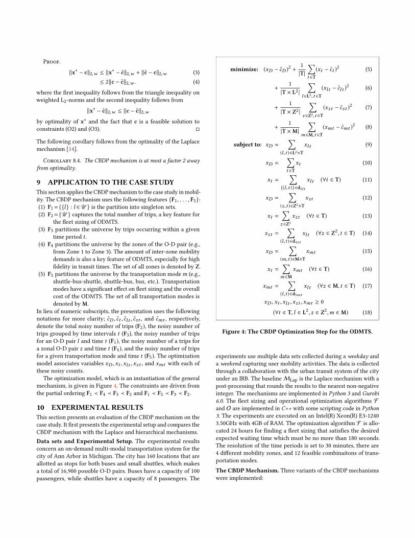
The optimization model, which is an instantiation of the general
mechanism, is given in Figure 4. The constraints are driven from
the partial ordering F1 ≺ F4 ≺ F3 ≺ F2 and F1 ≺ F5 ≺ F3 ≺ F2.
10 EXPERIMENTAL RESULTSThis section presents an evaluation of the CBDP mechanism on the
case study. It first presents the experimental setup and compares the
CBDP mechanism with the Laplace and hierarchical mechanisms.
Data sets and Experimental Setup. The experimental results
concern an on-demand multi-modal transportation system for the
city of Ann Arbor in Michigan. The city has 160 locations that are
allotted as stops for both buses and small shuttles, which makes
a total of 16,900 possible O-D pairs. Buses have a capacity of 100
passengers, while shuttles have a capacity of 8 passengers. The
minimize: (xD − c̃D )2 +
1
|T|
∑t ∈T
(xt − c̃t )2
(5)
+1
|T × L2 |
∑l ∈L2,t ∈T
(xl t − c̃l t )2
(6)
+1
|T × Z2 |
∑z∈Z2,t ∈T
(xzt − c̃zt )2
(7)
+1
|T ×M|
∑m∈M,t ∈T
(xmt − c̃mt )2
(8)
subject to: xD =∑
(l,t )∈L2×T
xl t (9)
xD =∑t ∈T
xt (10)
xt =∑
{(l,t )}∈d3l t
xl t (∀t ∈ T) (11)
xD =∑
(z,t )∈Z2×T
xzt (12)
xt =∑z∈Z2
xzt (∀t ∈ T) (13)
xzt =∑
(l,t )∈d4zt
xl t (∀z ∈ Z2, t ∈ T) (14)
xD =∑
(m,t )∈M×T
xmt (15)
xt =∑m∈M
xmt (∀t ∈ T) (16)
xmt =∑
(l,t )∈d5mt
xl t (∀z ∈ M, t ∈ T) (17)
xD , xt ,xl t ,xzt ,xmt ≥ 0
(∀t ∈ T, l ∈ L2, z ∈ Z2,m ∈ M) (18)
Figure 4: The CBDP Optimization Step for the ODMTS.
experiments use multiple data sets collected during a weekday and
a weekend capturing user mobility activities. The data is collected
through a collaboration with the urban transit system of the city
under an IRB. The baseline MLap is the Laplace mechanism with a
post-processing that rounds the results to the nearest non-negative
integer. The mechanisms are implemented in Python 3 and Gurobi6.0. The fleet sizing and operational optimization algorithms F
and O are implemented in C++ with some scripting code in Python3. The experiments are executed on an Intel(R) Xeon(R) E3-1240
3.50GHz with 4GB of RAM. The optimization algorithm F is allo-
cated 24 hours for finding a fleet sizing that satisfies the desired
expected waiting time which must be no more than 180 seconds.
The resolution of the time periods is set to 30 minutes, there are
4 different mobility zones, and 12 feasible combinaitons of trans-
portation modes.
The CBDPMechanism. Three variants of the CBDP mechanisms
were implemented:
(a) (b)
(c) (d)
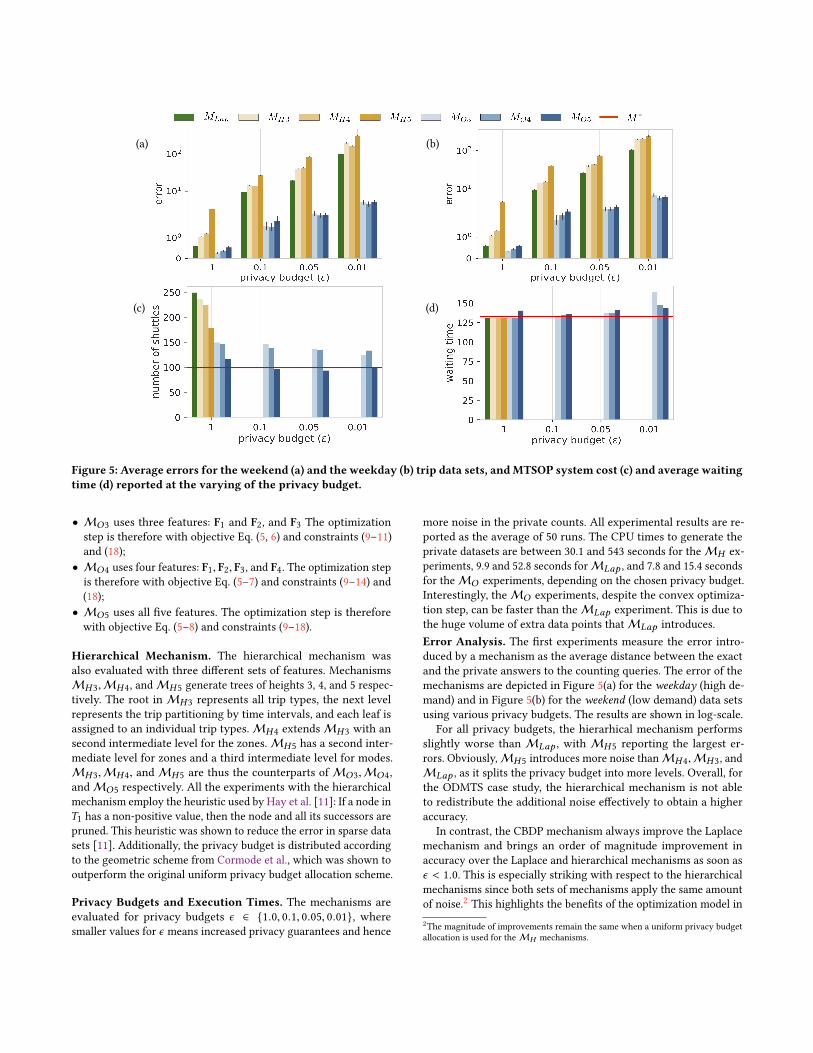
Figure 5: Average errors for the weekend (a) and the weekday (b) trip data sets, andMTSOP system cost (c) and average waitingtime (d) reported at the varying of the privacy budget.
• MO3 uses three features: F1 and F2, and F3 The optimization
step is therefore with objective Eq. (5, 6) and constraints (9–11)
and (18);
• MO4 uses four features: F1, F2, F3, and F4. The optimization step
is therefore with objective Eq. (5–7) and constraints (9–14) and
(18);
• MO5 uses all five features. The optimization step is therefore
with objective Eq. (5–8) and constraints (9–18).
Hierarchical Mechanism. The hierarchical mechanism was
also evaluated with three different sets of features. Mechanisms
MH3,MH4, and MH5 generate trees of heights 3, 4, and 5 respec-
tively. The root in MH3 represents all trip types, the next level
represents the trip partitioning by time intervals, and each leaf is
assigned to an individual trip types. MH4 extends MH3 with an
second intermediate level for the zones.MH5 has a second inter-
mediate level for zones and a third intermediate level for modes.
MH3,MH4, and MH5 are thus the counterparts of MO3,MO4,
andMO5 respectively. All the experiments with the hierarchical
mechanism employ the heuristic used by Hay et al. [11]: If a node in
T1 has a non-positive value, then the node and all its successors are
pruned. This heuristic was shown to reduce the error in sparse data
sets [11]. Additionally, the privacy budget is distributed according
to the geometric scheme from Cormode et al., which was shown to
outperform the original uniform privacy budget allocation scheme.
Privacy Budgets and Execution Times. The mechanisms are
evaluated for privacy budgets ϵ ∈ {1.0, 0.1, 0.05, 0.01}, where
smaller values for ϵ means increased privacy guarantees and hence
more noise in the private counts. All experimental results are re-
ported as the average of 50 runs. The CPU times to generate the
private datasets are between 30.1 and 543 seconds for the MH ex-
periments, 9.9 and 52.8 seconds forMLap , and 7.8 and 15.4 seconds
for the MO experiments, depending on the chosen privacy budget.
Interestingly, the MO experiments, despite the convex optimiza-
tion step, can be faster than theMLap experiment. This is due to
the huge volume of extra data points thatMLap introduces.
Error Analysis. The first experiments measure the error intro-
duced by a mechanism as the average distance between the exact
and the private answers to the counting queries. The error of the
mechanisms are depicted in Figure 5(a) for the weekday (high de-
mand) and in Figure 5(b) for the weekend (low demand) data sets
using various privacy budgets. The results are shown in log-scale.
For all privacy budgets, the hierarhical mechanism performs
slightly worse than MLap , with MH5 reporting the largest er-
rors. Obviously,MH5 introduces more noise thanMH4,MH3, and
MLap , as it splits the privacy budget into more levels. Overall, for
the ODMTS case study, the hierarchical mechanism is not able
to redistribute the additional noise effectively to obtain a higher
accuracy.
In contrast, the CBDP mechanism always improve the Laplace
mechanism and brings an order of magnitude improvement in
accuracy over the Laplace and hierarchical mechanisms as soon as
ϵ < 1.0. This is especially striking with respect to the hierarchical
mechanisms since both sets of mechanisms apply the same amount
of noise.2This highlights the benefits of the optimization model in
2The magnitude of improvements remain the same when a uniform privacy budget
allocation is used for the MH mechanisms.
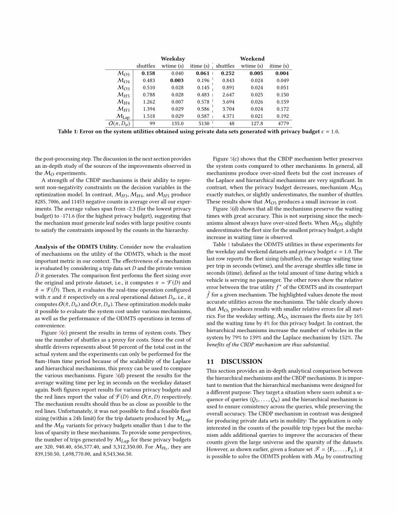
Weekday Weekendshuttles wtime (s) itime (s) shuttles wtime (s) itime (s)
MO5 0.158 0.040 0.061 0.252 0.005 0.004MO4 0.483 0.003 0.196 0.843 0.024 0.049
MO3 0.510 0.028 0.145 0.891 0.024 0.051
MH5 0.788 0.028 0.483 2.647 0.025 0.150
MH4 1.262 0.007 0.578 3.694 0.026 0.159
MH3 1.394 0.029 0.586 3.704 0.024 0.172
MLap 1.518 0.029 0.587 4.371 0.021 0.192
O(π ,Do ) 99 135.0 5130 48 127.8 4779
Table 1: Error on the system utilities obtained using private data sets generated with privacy budget ϵ = 1.0.
the post-processing step. The discussion in the next section provides
an in-depth study of the sources of the improvements observed in
the MO experiments.
A strength of the CBDP mechanisms is their ability to repre-
sent non-negativity constraints on the decision variables in the
optimization model. In contrast, MH3,MH4, and MH5 produce
8285, 7006, and 11453 negative counts in average over all our exper-
iments. The average values span from -2.3 (for the lowest privacy
budget) to -171.6 (for the highest privacy budget), suggesting that
the mechanism must generate leaf nodes with large positive counts
to satisfy the constraints imposed by the counts in the hierarchy.
Analysis of the ODMTS Utility. Consider now the evaluation
of mechanisms on the utility of the ODMTS, which is the most
important metric in our context. The effectiveness of a mechanism
is evaluated by considering a trip data set D and the private version
D̃ it generates. The comparison first performs the fleet sizing over
the original and private dataset, i.e., it computes π = F (D) andπ̃ = F (D̃). Then, it evaluates the real-time operation configured
with π and π̃ respectively on a real operational dataset Do , i.e., it
computes O(π̃ ,Do ) and O(π ,Do ). These optimization models make
it possible to evaluate the system cost under various mechanisms,
as well as the performance of the ODMTS operations in terms of
convenience.
Figure 5(c) present the results in terms of system costs. They
use the number of shuttles as a proxy for costs. Since the cost of
shuttle drivers represents about 50 percent of the total cost in the
actual system and the experiments can only be performed for the
8am-10am time period because of the scalability of the Laplace
and hierarchical mechanisms, this proxy can be used to compare
the various mechanisms. Figure 5(d) present the results for the
average waiting time per leg in seconds on the weekday dataset
again. Both figures report results for various privacy budgets and
the red lines report the value of F (D) and O(π ,D) respectively.The mechanism results should thus be as close as possible to the
red lines. Unfortunately, it was not possible to find a feasible fleet
sizing (within a 24h limit) for the trip datasets produced by MLapand theMH variants for privacy budgets smaller than 1 due to the
loss of sparsity in these mechanisms. To provide some perspectives,
the number of trips generated by MLap for these privacy budgets
are 320, 940.40, 656,577.40, and 3,312,350.00. For MH5, they are
839,150.50, 1,698,770.00, and 8,543,366.50.
Figure 5(c) shows that the CBDP mechanism better preserves
the system costs compared to other mechanisms. In general, all
mechanisms produce over-sized fleets but the cost increases of
the Laplace and hierarchical mechanisms are very significant. In
contrast, when the privacy budget decreases, mechanism MO5
exactly matches, or slightly underestimates, the number of shuttles.
These results show thatMO5 produces a small increase in cost.
Figure 5(d) shows that all the mechanisms preserve the waiting
times with great accuracy. This is not surprising since the mech-
anisms almost always have over-sized fleets. WhenMO5 slightly
underestimates the fleet size for the smallest privacy budget, a slight
increase in waiting time is observed.
Table 1 tabulates the ODMTS utilities in these experiments for
the weekday and weekend datasets and privacy budget ϵ = 1.0. The
last row reports the fleet sizing (shuttles), the average waiting time
per trip in seconds (wtime), and the average shuttles idle time in
seconds (itime), defined as the total amount of time during which a
vehicle is serving no passenger. The other rows show the relative
error between the true utility f ∗ of the ODMTS and its counterpart
˜f for a given mechanism. The highlighted values denote the most
accurate utilities across the mechanisms. The table clearly shows
thatMO5produces results with smaller relative errors for all met-
rics. For the weekday setting, MO5increases the fleets size by 16%
and the waiting time by 4% for this privacy budget. In contrast, the
hierarchical mechanisms increase the number of vehicles in the
system by 79% to 139% and the Laplace mechanism by 152%. Thebenefits of the CBDP mechanism are thus substantial.
11 DISCUSSIONThis section provides an in-depth analytical comparison between
the hierarchical mechanisms and the CBDPmechanisms. It is impor-
tant to mention that the hierarchical mechanisms were designed for
a different purpose: They target a situation where users submit a se-
quence of queries ⟨Q1, . . . ,Qn⟩ and the hierarchical mechanism is
used to ensure consistency across the queries, while preserving the
overall accuracy. The CBDP mechanism in contrast was designed
for producing private data sets in mobility: The application is only
interested in the counts of the possible trip types but the mecha-
nism adds additional queries to improve the accuracies of these
counts given the large universe and the sparsity of the datasets.
However, as shown earlier, given a feature set F = {F1, . . . , Fk }, itis possible to solve the ODMTS problem with MH by constructing

a hierarchy where F2 describes the root node, F1 the leaf nodes, andthe node for intermediate level i are the elements of the feature set
Fk−i+1. Thus, both methods make use of an optimization step to
post-process the counting queries, althoughMH "solves" a relaxed
version of the problem using a closed-form solution (relaxing the
non-negativity constraints), while MO solves an actual convex
optimization problem. There are three key aspects that differentiate
the CBDP from the hierarchical method:
1. The Problem Structure. The CBDP and hierarchical mecha-
nisms imposed a fundamentally different structure on the con-
straints of the optimization model: flat (F) or hierarchical (H). The
flat structure imposed by MO allows each element of a feature set
to be related via a constraint to any set of elements of any other
feature set. The hierarchical structure used by MH imposes a hier-
archy on the elements of the feature set so that children counts are
related to the parent counts. This has an important consequence
on the number of total queries the mechanisms need to answer. In
the flat representation, the mechanism requires at most
∑Fi ∈F |Fi |
queries while, in the hierarchical representation, a mechanism re-
quires
∏Fi ∈F |Fi | queries. Imposing a hierarchical structure has
also an important consequence on the amount of decision variables
and constraints of the optimization model. The program requires
a variable for each count associated with a node, i.e.,
∏Fi ∈F |Fi |
variables. In contrast, a flat structure requires
∑Fi ∈F |Fi | variables.
The same consideration holds for constraints. These quantities neg-
atively and dramatically affect the performance of a hierarchical
organization for the optimization method, hindering its scalability.
2. Non-Negative Variables. The CBDP mechanism naturally han-
dles the negative outputs from the Laplace mechanism via post-processing. In contrast, the hierarchical mechanism’s closed-form
solution ignores the nonnegativity constraints. Such property is
especially important for counting queries on sparse datasets, as in
the ODMTS case study.
3. Weighted Distance. The CBDP mechanism also optimizes a
weighted L2-norm, which ensures that each feature contributes
equally to the objective. This is important since they all are parti-
tions of the same universe.
Impact Evaluation. These three aspects are now evaluated on the
case study. In addition to MO5 and MH5, the following variants
ofMO5 are considered:
• MO5(a) uses a hierarchical structure in the constraints, non-
negative decision variables, and uniform weights for the terms
in the objective.
• MO5(b) uses a hierarchical structure in the constraints, non-
negative decision variables, and the weighting scheme ofMO5.
• MO5(c) uses a flat structure, non-negative decision variables,
and a uniform weighting scheme.
Table 2 tabulates the errors introduced by the mechanisms as in
Figures 5(a–b), i.e., the average distance between the exact and the
private answers to the counting queries. The columns S, P, and W,
respectively, denote the type of structure adopted by the mecha-
nism (F or H), whether the optimization uses non-negative valued
variables, and whether a weighting scheme is used for the optimiza-
tion. The results clearly indicate that all three aspects are critical
for the required accuracy and demonstrate the superiority of the
combination adopted by MO5. The second line shows that the
Prop Privacy budgetWeekday Weekend
S P W 1.0 0.1 0.01 1.0 0.1 0.01
MO5 F ✓ ✓ 0.91 3.87 6.01 0.86 2.69 5.77MH5 H ✗ ✗ 5.11 56.6 715 4.57 50.9 728
MO5(a) H ✓ ✗ 35.6 44.2 108 42.2 59.9 120.5
MO5(b) H ✓ ✓ 13.4 15.7 18.9 13.4 14.5 19.6
MO5(c) F ✓ ✗ 1.50 5.55 15.2 1.34 4.27 18.4
Table 2: Analysis of the Key Features of CBDP.
performance of the hierarchical mechanism significantly degrades
when the privacy budget decreases: The magnitude of its errors are
more than 5, 14, and 118 times larger from weekdays thanMO5 for
privacy budgets 1.0, 0.1, and 0.01. MechanismMO5(a) shows thatadding the non-negativity constraints is helpful in slowing down
the performance degradation as the privacy budget decreases but
the errors remain more than an order of magnitude larger than
MO5. Mechanism MO5(b) indicates the importance of a flat struc-
ture in the optimization: For privacy budgets 1.0 and 0.1, the errors
introduced by a hierarchical structure are an order of magnitude
larger than those with a flat structure. Finally, mechanism MO5(c)demonstrates the benefits of the weighted objective as the privacy
budget decreases: For a budget of 0.01, the weighting scheme de-
creases the errors by a factor of about 2.5 in weekdays. This analysis
clearly demonstrates the benefits of the CBDP mechanism for mo-
bility applications.
12 CONCLUSIONSThis paper introduced Constraint-Based Differential Privacy
(CBDP), an approach to differential privacy which aims at releasing
private mobility data set for complex optimization tasks. CBDP
casts the private data set release as an optimization problem that
redistributes the noise introduced by a randomized mechanism to
satisfy fundamental constraints of the original data. The optimiza-
tionmodelminimizes aweighted L2-norm between the noisy counts
generated by the Laplace mechanism and post-processed counts
that satisfy constraints imposed by the features of the application.
CBDP has been evaluated on several mobility datasets for the
city of Ann Arbor, MI, and the design and operations of an On-
Demand Multimodal Transit System (ODMTS). Experimental re-
sults show that CBDP improves the accuracy of existing approaches
(the Laplace mechanism and hierarchical mechanisms) by an order
of magnitude and results in negligible utility losses compared to an
ODMTS designed with the actual data. These results are promising
and indicates that CBDP has the potential to become an important
tool at the intersection of privacy, mobility, and optimization.
Although the paper focused on the applicability of CBDP to
ODMTS, the proposed mechanism is general and can be used for
other applications where data features and/or knowledge of the
problem of interest is available.
ACKNOWLEDGMENTSThis work was partially supported by the Michigan Institute of
Data Science and the Seth Bonder Foundation.

REFERENCES[1] Alastair R Beresford and Frank Stajano. 2003. Location privacy in pervasive
computing. IEEE Pervasive computing 2, 1 (2003), 46–55.
[2] Graham Cormode, Cecilia Procopiuc, Divesh Srivastava, Entong Shen, and Ting
Yu. 2012. Differentially private spatial decompositions. InData engineering (ICDE),2012 IEEE 28th international conference on. IEEE, 20–31.
[3] GrahamCormode, Magda Procopiuc, Divesh Srivastava, and Thanh TL Tran. 2011.
Differentially private publication of sparse data. arXiv preprint arXiv:1103.0825(2011).
[4] Yves-Alexandre De Montjoye, César A Hidalgo, Michel Verleysen, and Vincent D
Blondel. 2013. Unique in the crowd: The privacy bounds of human mobility.
Scientific reports 3 (2013), 1376.[5] Bolin Ding, Marianne Winslett, Jiawei Han, and Zhenhui Li. 2011. Differentially
private data cubes: optimizing noise sources and consistency. In Proceedings ofthe 2011 ACM SIGMOD International Conference on Management of data. ACM,
217–228.
[6] Cynthia Dwork, Frank McSherry, Kobbi Nissim, and Adam Smith. 2006. Cali-
brating noise to sensitivity in private data analysis. In TCC, Vol. 3876. Springer,265–284.
[7] Cynthia Dwork, Aleksandar Nikolov, and Kunal Talwar. 2015. Efficient algorithms
for privately releasingmarginals via convex relaxations. Discrete & ComputationalGeometry 53, 3 (2015), 650–673.
[8] Cynthia Dwork and Aaron Roth. 2013. The algorithmic foundations of differential
privacy. Theoretical Computer Science 9, 3-4 (2013), 211–407.[9] Ferdinando Fioretto and Pascal Van Hentenryck. 2018. Constrained-based Differ-
ential Privacy: Releasing Optimal Power Flow Benchmarks Privately. In Proceed-ings of the International Conference on the Integration of Constraint Programming,Artificial Intelligence, and Operations Research (CPAIOR).
[10] Marco Gruteser and Xuan Liu. 2004. Protecting privacy, in continuous location-
tracking applications. IEEE Security & Privacy 2, 2 (2004), 28–34.
[11] Michael Hay, Vibhor Rastogi, Gerome Miklau, and Dan Suciu. 2010. Boosting the
accuracy of differentially private histograms through consistency. Proceedings ofthe VLDB Endowment 3, 1-2 (2010), 1021–1032.
[12] Justin Hsu, Marco Gaboardi, Andreas Haeberlen, Sanjeev Khanna, Arjun Narayan,
Benjamin C Pierce, and Aaron Roth. 2014. Differential privacy: An economic
method for choosing epsilon. In Computer Security Foundations Symposium (CSF),
2014 IEEE 27th. IEEE, 398–410.[13] Dong Huang, Shuguo Han, Xiaoli Li, and Philip S Yu. 2015. Orthogonal mecha-
nism for answering batch queries with differential privacy. In Proceedings of the27th International Conference on Scientific and Statistical Database Management.ACM, 24.
[14] Fragkiskos Koufogiannis, Shuo Han, and George J Pappas. 2015. Optimality of
the laplace mechanism in differential privacy. arXiv preprint arXiv:1504.00065(2015).
[15] John Krumm. 2009. A survey of computational location privacy. Personal andUbiquitous Computing 13, 6 (2009), 391–399.
[16] Chao Li, Michael Hay, GeromeMiklau, and YueWang. 2014. A data-andworkload-
aware algorithm for range queries under differential privacy. Proceedings of theVLDB Endowment 7, 5 (2014), 341–352.
[17] Tiancheng Li and Ninghui Li. 2009. On the tradeoff between privacy and utility in
data publishing. In Proceedings of the 15th ACM SIGKDD international conferenceon Knowledge discovery and data mining. ACM, 517–526.
[18] Yang D Li, Zhenjie Zhang, Marianne Winslett, and Yin Yang. 2011. Compressive
mechanism: Utilizing sparse representation in differential privacy. In Proceedingsof the 10th annual ACM workshop on Privacy in the electronic society. ACM, 177–
182.
[19] Arthur Maheo, Phlip Kilby, and Pascal Van Hentenryck. 2017. Benders Decompo-
sition for the Design of a Hub and Shuttle Public Transit System. TransportationScience (2017). To appear.
[20] Arkadi Nemirovski. 2004. Interior Point Polynomial Time Methods IN ConvexProgramming. Technical Report ISYE 8813. Georgia Institute of Technology,
Atlanta, GA.
[21] Wahbeh Qardaji, Weining Yang, and Ninghui Li. 2013. Understanding hierarchical
methods for differentially private histograms. Proceedings of the VLDB Endowment6, 14 (2013), 1954–1965. http://www.vldb.org/pvldb/vol6/p1954-qardaji.pdf
[22] Wahbeh Qardaji, Weining Yang, and Ninghui Li. 2014. PriView: practical differ-
entially private release of marginal contingency tables. In Proceedings of the 2014ACM SIGMOD international conference on Management of data. ACM, 1435–1446.
[23] Salil Vadhan. 2017. The complexity of differential privacy. In Tutorials on theFoundations of Cryptography. Springer, 347–450.
[24] Xiaokui Xiao, Guozhang Wang, and Johannes Gehrke. 2011. Differential privacy
via wavelet transforms. IEEE Transactions on Knowledge and Data Engineering23, 8 (2011), 1200–1214.