conservation assessment of greater sage-grouse and
TRANSCRIPT

Conservation Assessment of Greater Sage-grouse
and Sagebrush Habitats
J. W. ConnellyS. T. KnickM. A. SchroederS. J. Stiver
Western Association of Fish and Wildlife Agencies
June 2004
i
CONSERVATION ASSESSMENT OFGREATER SAGE-GROUSE and SAGEBRUSH HABITATS
John W. ConnellyIdaho Department Fish and Game
83 W 215 NBlackfoot, ID 83221
Steven T. KnickUSGS Forest & Rangeland Ecosystem Science Center
Snake River Field Station970 Lusk St.
Boise, ID [email protected]
Michael A. SchroederWashington Department of Fish and Wildlife
P.O. Box 1077Bridgeport, WA 98813
San J. StiverWildlife Coordinator,
National Sage-Grouse Conservation Framework Planning Team2184 Richard St.
Prescott, AZ [email protected]
This report should be cited as:
Connelly, J. W., S. T. Knick, M. A. Schroeder, and S. J. Stiver. 2004. Conservation Assessmentof Greater Sage-grouse and Sagebrush Habitats. Western Association of Fish andWildlife Agencies. Unpublished Report. Cheyenne, Wyoming.
Cover photo credit, Kim Toulouse
Conservation Assessment of Greater Sage-grouse and Sagebrush Habitats Connelly et al.
ii
Author Biographies
John W. Connelly
Jack has been employed as a Principal Wildlife Research Biologist with the IdahoDepartment of Fish and Game for the last 20 years. He received his B.S. degree from theUniversity of Idaho and M.S. and Ph.D. degrees from Washington State University. Jack is aCertified Wildlife Biologist and works on grouse conservation issues at national andinternational scales. He is a member of the Western Sage and Columbian Sharp-tailed TechnicalCommittee and the Grouse Specialists’ Group. Jack has been involved with sage-grouseresearch and management issues for over 27 years.
Steven T. Knick
Steve has been employed as a federal Research Ecologist since 1990, most recently withthe United States Geological Survey. He received his B.S. degree from the University ofMinnesota, M.S. from Washington State University and Ph.D. from the University of Montana.Steve has worked on national and international wildlife issues ranging from wolf and grizzlybear management to conservation of shrubland ecosystems. For the past 15 years, Steve hasintegrated field and GIS-based analyses to study the effects of disturbance on sagebrush habitatsand bird communities.
Michael A. Schroeder
Mike has been employed as the Upland Bird Research Biologist with the WashingtonDepartment of Fish and Wildlife for the last 12 years. He received his B.S. degree from TexasA&M University, M.S. from the University of Alberta, and Ph.D. from Colorado StateUniversity. Mike is a Certified Wildlife Biologist and works on grouse conservation issues atnational and international scales. He is a member of the Western Sage and Columbian Sharp-tailed Technical Committee and the Grouse Specialists’ Group. Mike has been involved withgrouse research and management issues for over 23 years.
San J. Stiver
San recently retired after 30 years as a biologist for the Nevada Division of Wildlife. Heis currently employed by the National Sage-Grouse Conservation Planning Framework Team.San received his B.S. from the University of Montana. He has been a member of the WildlifeSociety since 1971 and was a member of the Western Sage and Columbian Sharp-tailed GrouseTechnical Committee from 1981 – 2003. San has been involved in national and internationalwildlife conservation issues since 1985. He has worked on sage-grouse as a field biologist,researcher and staff biologist for over 25 years.
Conservation Assessment of Greater Sage-grouse and Sagebrush Habitats Connelly et al.
iii
Contributors
The following individuals provided important information and in many cases wrote portions ofone or more chapters.
Jenny BarnettHandford Reach National Monument/Saddle Mountain NWR3250 Port of Benton Blvd.Richland, WA 99352
Jenny Barnett, After studying sage grouse for her Master's degree, Jenny Barnett has worked as a wildlife biologistfor BLM and USFWS. Her work has focused on sage grouse, song birds, pygmy rabbits and other species inshrub-steppe habitat. She is currently a Wildlife Biologist/GIS specialist for Hanford Reach National Monument.
Erik A. BeeverUSGS Forest and Rangeland Ecosystem Science Center3200 SW Jefferson WayCorvallis, OR 97331email: [email protected]
Erik Beever, is a postdoctoral ecologist with the USGS-BRD Forest and Rangeland Ecosystem Science Center. Hehas studied the interactions of free-roaming horses and burros with other ecosystem components since 1995. Hisinterests include community ecology, wildlife biology, disturbance ecology (including climate change), andconservation of Great Basin habitats and landscapes.
Tom ChristiansenSage-Grouse Program CoordinatorWyoming Game and Fish Dept.351 Astle Ave.Green River, WY [email protected] Tom Christiansen, is the Sage-Grouse Program Coordinator for the Wyoming Game and Fish Department. Prior tothis appointment he was a regional wildlife biologist in Green River and has been with the WGF for 19 years.Christiansen received his Bachelor of Science degree from the University of Nebraska-Lincoln.
Michelle Commons-KemnerSenior Wildlife Research BiologistIdaho Department of Fish and Game3101 S. Powerline RoadNampa, Idaho [email protected]
Michelle Commons-Kemner, graduated with her under-graduate degree from the University of Northern Colorado,Greeley, and her Master's from the University of Manitoba, Canada. She conducted her thesis research on Gunnisonsage-grouse. Prior to being employed with IDFG she studied White-tailed ptarmigan in Colorado and VancouverIsland. She has been employed with IDFG since 1998, and as a sage-grouse research biologist since 2000. Shecontinues to be actively involved in the sage-grouse research projects across the state as well as working on Idaho'sGreater sage-grouse conservation plan, and developing new sage-grouse Local Working Groups.

Conservation Assessment of Greater Sage-grouse and Sagebrush Habitats Connelly et al.
iv
Sean FinnUSGS Forest & Rangeland Ecosystem Science CenterSnake River Field Station970 Lusk St.Boise, ID [email protected]
Sean Finn, received his M.S. in Raptor Biology from Boise State University in 2000. His thesis project examinedthe influences of habitat quality and scale of investigation on Northern Goshawk breeding ecology on the OlympicPeninsula. He is currently employed as a Wildlife Biologist for the USGS Biological Resources Division workingon avian conservation issues in western shrub-steppe landscapes.
Scott GardnerCalifornia Department of Game and FishWildlife Programs Branch1812 9th StreetSacramento, CA [email protected]
Scott Gardner, is the sage grouse coordinator for the California Department of Fish and Game. Scott received hisM.S. in Wildlife Resources from the University of Idaho, where he worked on reintroduction of Columbian sharp-tailed grouse and sage grouse research in southeastern Idaho. Scott is currently leading sage grouse conservationplanning efforts in California and collaborating on research projects statewide.
Edward O. GartonProfessorFish and Wildlife ResourcesUniversity of IdahoMoscow, ID [email protected]
Edward O. Garton, is a professor at the University of Idaho with joint appointments in Wildlife Ecology andStatistics. He and his students have been studying the population ecology of both rare and abundant birds andmammals in the Western U.S. for the past 30 years. They have published more than 50 papers and monographs onspecies ranging from white-crowned sparrows to elk with additional contributions developing quantitative tools forassessing home range/space use, abundance of song birds and dynamics of large mammals using aerial surveys.
Michael GreggLand Management and Research Demonstration BiologistHanford Reach National Monument and Saddle Mountain National Wildlife RefugeU.S. Fish and Wildlife Service3720 Port of Benton Blvd.Richland, WA [email protected]
Michael Gregg, B.S. 1985 Humboldt State University, M.S. 1991 (on sage grouse) Oregon state University, Ph.DCandidate (on sage grouse) Oregon State University. Mike has 15 years experience with sage-grouse and 11 yearswith the USFWS. He is currently the Land Management and Research Demonstration Biologist for Region 1 andcoordinates and conduct research and restoration projects in shrub-steppe and on sagebrush dependent wildlife.

Conservation Assessment of Greater Sage-grouse and Sagebrush Habitats Connelly et al.
v
Steven HanserUSGS Forest & Rangeland Ecosystem Science CenterSnake River Field Station970 Lusk St.Boise, ID [email protected]
Steve Hanser, is a Wildlife Biologist at the USGS Snake River Field Station in Boise, Idaho. Steve received hisM.S. in Biological Sciences and Geotechnologies Post-baccalaureate Certification in 2002 from Idaho StateUniversity where he studied the impact of habitat fragmentation on the shrub-steppe small mammal community ofeastern Idaho. His current work includes GIS/remote sensing analysis and modeling for several projects studyinglandscape-scale issues in the sagebrush ecosystem.
Matthew J. HolloranWyoming Cooperative Research UnitUniversity of WyomingBox 3166 University StationLaramie, WY [email protected]
Matthew Holloran, has been doing research on sage-grouse in Wyoming since 1997, and is currently working on hisdissertation investigating the potential impacts of natural gas development on sage-grouse in western Wyoming.
Matthias LeuUSGS Forest & Rangeland Ecosystem Science CenterSnake River Field Station970 Lusk St.Boise, ID [email protected]
Matthias Leu, is a postdoctoral associate with USGS in Boise, ID. He earned a PhD from the University ofWashington in wildlife biology and conservation; his dissertation work investigated habitat-wildlife interactions. Asa post doctoral fellow, Matthias worked with John Marzluff, University of Washington, on models predicting thespatial distribution of marbled murrelet nest predators and currently investigates with Steve Knick, at USGS in BoiseID, how anthropogenic resources and land cover change influence sagebrush habitats and wildlife populations.Matthias’ research interests are in spatial ecology and wildlife conservation.
Alison Holloran (Lyon)Wyoming Audubon168 N. Cedar StreetLaramie, WY [email protected]
Alison Holloran, is originally from Baltimore area of Maryland but has been in Laramie, WY for last seven yearswhere she serves as Conservation Coordinator for Audubon Wyoming. Alison earned her BS in WildlifeManagement from West Virginia University and a MS from the University of Wyoming in Zoology and Physiology.She served 2 1/2 years for the Peace Corp in Honduras. Alison is married with a new little girl- Sage Marie.

Conservation Assessment of Greater Sage-grouse and Sagebrush Habitats Connelly et al.
vi
Cara MeinkeUSGS Forest & Rangeland Ecosystem Science CenterSnake River Field Station970 Lusk St.Boise, ID [email protected]
Cara Meinke, is a wildlife biologist specializing in special data analysis and management for the United StatesGeological Service, Snake River Field Station. She has spent the last 2 ½ years working on the SAGEMAP andPRAIRIEMAP projects as a special analyst on various ecoregional assessments in the sagebrush-steppe biome.
Rick MillerOregon State University67826-A Hwy 205Burns, [email protected]
Rick Miller, has been a range ecology professor at Oregon State University since 1977. He has worked on sagebrushand juniper systems for the past 28 years with emphasis on succession and fire.
Rick NorthrupState Bird Coordinator Montana Fish, Wildlife & ParksP.O. Box 200701Helena, MT [email protected]
Rick Northrup, earned his B.S. degree from South Dakota State University and his M.S. from Montana StateUniversity where he studied sharp-tailed grouse habitat use during fall and winter on the Charles M. RussellNational Wildlife Refuge.
Sara Oyler-McCanceRocky Mountain Center for Conservation Genetics and SystematicsUSGSDepartment of Biological SciencesUniversity of DenverDenver, CO [email protected]
Sara Oyler-McCance, is the co-director of the Rocky Mountain Center for Conservation Genetics and Systematics inDenver, CO. She has worked as a conservation geneticist for USGS for 5 years. Prior to this position, Sara receivedher PhD in Fishery and Wildlife Biology from Colorado State University where she studied different aspects ofGunnison Sage-Grouse ecology.

Conservation Assessment of Greater Sage-grouse and Sagebrush Habitats Connelly et al.
vii
David PykeUSGS, Forest & Rangeland Ecosystem Science Center3200 SW Jefferson WayCorvallis, OR [email protected]
David Pyke, is a Research Rangeland Ecologist who is currently conducting research studies on the plant populationand community ecology in sagebrush/grass ecosystems of the northern Great Basin. He is also conducting studies onchanges in ecosystem processes when cheatgrass dominates sagebrush communities. He has current studiesinvolving control of cheatgrass and restoration of sagebrush grass communities.
Tom W. QuinnAssociate ProfessorDepartment of Biological SciencesUniversity of DenverDenver, CO 80208Co-director,Rocky Mountain Center for Conservation Genetics and [email protected]
Tom Quinn, has been using molecular techniques for studies of evolution, systematics, and population genetics forover 20 years. He discovered the occurrence of nuclear copies of mitochondrial sequences in the nuclear genome ofbirds, and his lab has tested hypotheses related to the "molecular clock hypothesis" and developed a molecularmethod for sexing most avian species.
Kerry P. ReeseDepartment of Fish and Wildlife ResourcesUniversity of IdahoMoscow, ID [email protected]
Kerry Reese, is currently chairman of the Department of Fish and Wildlife Resources at University of Idaho. Hismain interests include avian ecology and management. He has been involved in research and management efforts onsage-grouse for over 17 years.
E. Thomas RinkesBureau of Land ManagementP.O. Box 589Lander, WY [email protected]
Tom Rinkes, is a sage-grouse/sagebrush species of concern biologist with the Wyoming State Office of the Bureau ofLand Management. He received his degree in wildlife resources from the University of Idaho. He has worked forthe BLM for the past 26 years in Wyoming and Idaho and has been involved in sage-grouse management since 1986.

Conservation Assessment of Greater Sage-grouse and Sagebrush Habitats Connelly et al.
viii
Mary M. RowlandWildlife BiologistUSDA Forest Service, PNW Research StationForestry and Range Sciences Laboratory1401 Gekeler LaneLa Grande, OR [email protected]
Mary Rowland, is a wildlife biologist for the U.S. Forest Service in La Grande, Oregon. She has worked on issuesrelated to sage-grouse and sagebrush for the last 5 years, both for the BLM and FS. This work has included writinga research problem analysis for Greater Sage-Grouse in Oregon and conducting regional assessments of sagebrushhabitats and species of concern for the BLM.
Linda SchueckUSGS Forest & Rangeland Ecosystem Science CenterSnake River Field Station970 Lusk St.Boise, ID [email protected]
Linda Schueck, is a Computer Specialist at the USGS Forest and Rangeland Ecosystem Science Center, Snake RiverField Station in Boise, Idaho. She is interested in computer programming for data transfer methods and for GISanalysis of biological information. Linda designed and programmed the USGS SAGEMAP website(http//:sagemap.wr.usgs.gov).
Sonja E. TaylorRocky Mountain Center for Conservation Genetics and SystematicsDepartment of Biological SciencesUniversity of DenverDenver, CO [email protected]
Sonja Taylor, has worked on a number of greater sage-grouse projects. Sonja has recently been collecting fragmentanalysis data in greater sage-grouse populations from throughout their range in North America. She also conductedpreliminary behavioral field work on a sage grouse population in California that was found to be genetically distinct.Additionally, using "ancient" DNA (100 years old), she has attempted to address some questions about the originand history of modern white-tailed kite populations.
Michael J. WisdomResearch Wildlife BiologistPacific Northwest Research Station1401 Gekeler LaneLa Grande, OR [email protected]
Mike Wisdom, has worked on a variety of wildlife research and management issues for the Bureau of LandManagement and Forest Service during the past 20 years. More recently, Mike has been involved in a variety ofregional assessments of habitats for sagebrush-associated species of conservation concern in the western UnitedStates. Mike received his Ph.D. in Forestry, Range, and Wildlife from the Univ. of Idaho, his M.S. in WildlifeScience from New Mexico St. Univ., and his B.S. in Wildlife Management from the Univ. Of Wisconsin-StevensPoint.

Conservation Assessment of Greater Sage-grouse and Sagebrush Habitats Connelly et al.
ix
Conservation Assessment of Greater Sage-grouse and Sagebrush Habitats
Table of Contents
AUTHORS ..................................................................................................................................... iCONTRIBUTING AUTHORS .................................................................................................... iiiACKNOWLEDGMENTS .......................................................................................................... xixEXECUTIVE SUMMARY ..................................................................................................... ES-1CHAPTER 1
INTRODUCTION ............................................................................................................... 1-1Range-wide Conservation Assessment .......................................................................... 1-1
Background and Rationale ....................................................................................... 1-1Objectives and Perspective of the Conservation Assessment .................................. 1-3Geographical, Temporal, Jurisdictional, and Scientific Scope ................................ 1-4Treatment of Uncertainty ......................................................................................... 1-6
Review of the Conservation Assessment ....................................................................... 1-7Criteria for Use of Data and Scientific Information ................................................ 1-7Documentation of Data and Sources ........................................................................ 1-8
Management and Stewardship of Sagebrush Habitats ................................................... 1-8Principal Legislation Governing the Management and Use of Public Lands .......... 1-8Stewardship of Sagebrush Lands ............................................................................. 1-9
Literature Cited ............................................................................................................ 1-10Figures ......................................................................................................................... 1-16Tables ........................................................................................................................... 1-23
CHAPTER 2CONSERVATION STATUS OF GREATER SAGE-GROUSE POPULATIONS ............ 2-1
Introduction .................................................................................................................... 2-1United States and Canadian Federal Laws .................................................................... 2-2State and Provincial Laws .............................................................................................. 2-2
Alberta ..................................................................................................................... 2-2California ................................................................................................................. 2-2Colorado ................................................................................................................... 2-3Idaho ........................................................................................................................ 2-4Montana ................................................................................................................... 2-5Nevada ..................................................................................................................... 2-5North Dakota ............................................................................................................ 2-6Oregon ...................................................................................................................... 2-7South Dakota ............................................................................................................ 2-8Utah ........................................................................................................................ 2-10Washington ............................................................................................................ 2-10Wyoming ................................................................................................................ 2-10

Conservation Assessment of Greater Sage-grouse and Sagebrush Habitats Connelly et al.
x
Sage-grouse Petitions ................................................................................................... 2-11State/Province Conservation Plans .............................................................................. 2-12
Coordination and Standards ................................................................................... 2-12U.S. Bureau of Land Management ........................................................................ 2-13Alberta ................................................................................................................... 2-14California ............................................................................................................... 2-15Colorado ................................................................................................................. 2-15Idaho ...................................................................................................................... 2-15Montana ................................................................................................................. 2-16Nevada ................................................................................................................... 2-17North Dakota .......................................................................................................... 2-19Oregon .................................................................................................................... 2-19Saskatchewan ......................................................................................................... 2-20South Dakota .......................................................................................................... 2-20Utah ........................................................................................................................ 2-20Washington ............................................................................................................ 2-22Wyoming ................................................................................................................ 2-22
Summary ...................................................................................................................... 2-24Literature Cited ............................................................................................................ 2-25Tables ........................................................................................................................... 2-27Figure ........................................................................................................................... 2-33
CHAPTER 3POPULATION ECOLOGY & CHARACTERISTICS ....................................................... 3-1
Taxonomy, Systematics, & General Description ........................................................... 3-1Food Habits .................................................................................................................... 3-2
General ..................................................................................................................... 3-2Spring ....................................................................................................................... 3-2Summer .................................................................................................................... 3-3Fall and Winter ........................................................................................................ 3-4
Seasonal Movement and Fidelity ................................................................................... 3-4Breeding Biology ........................................................................................................... 3-6
Mating System ......................................................................................................... 3-6Territoriality ............................................................................................................. 3-7Physical Interactions ................................................................................................ 3-8Courtship ................................................................................................................. 3-8Timing of Breeding Behavior .................................................................................. 3-9
Nesting ......................................................................................................................... 3-10General Characteristics .......................................................................................... 3-10Nest Placement ....................................................................................................... 3-10Nest Likelihood ...................................................................................................... 3-10Nest Success .......................................................................................................... 3-11
Survival and Population Dynamics .............................................................................. 3-11

Conservation Assessment of Greater Sage-grouse and Sagebrush Habitats Connelly et al.
xi
Literature Cited ............................................................................................................ 3-12Tables ........................................................................................................................... 3-20
CHAPTER 4GREATER SAGE-GROUSE HABITAT CHARACTERISTICS ....................................... 4.1
Introduction .................................................................................................................... 4-1Breeding Habitats .......................................................................................................... 4-2
Leks .......................................................................................................................... 4-2General Description ........................................................................................... 4-2Specific Description ........................................................................................... 4-3Relevant Features ............................................................................................... 4-4
Nesting ..................................................................................................................... 4-4General Description ........................................................................................... 4-4Specific Description ........................................................................................... 4-5Relevant Features ............................................................................................... 4-6
Early Brood-rearing ................................................................................................. 4-8General Description ........................................................................................... 4-8Specific Description ........................................................................................... 4-8Relevant Features ............................................................................................... 4-9
Summer and Late Brood-Rearing Habitats .................................................................... 4-9General Description ................................................................................................. 4-9Seasonal Differences .............................................................................................. 4-10Specific Description ............................................................................................... 4-11Relevant Features ................................................................................................... 4-12
Autumn Habitats .......................................................................................................... 4-12Winter Habitats ............................................................................................................ 4-13
General Description ............................................................................................... 4-13Specific Description ............................................................................................... 4-14Relevant Features ................................................................................................... 4-14
Landscape Context Issues ............................................................................................ 4-15General Description ............................................................................................... 4-15Mosaics, Juxtaposition, and Diversity ................................................................... 4-17Migratory Corridors ............................................................................................... 4-18
Literature Cited ............................................................................................................ 4-19
CHAPTER 5SAGEBRUSH ECOSYSTEMS: DYNAMICS OF PRIMARY SAGEBRUSH HABITATS ................................................. 5-1DELINEATION AND DESCRIPTION OF SAGEBRUSH HABITATS ........................... 5-1
Introduction .............................................................................................................. 5-1Intermountain Region: Sagebrush Taxa .................................................................. 5-2
Northern Great Plains: Sagebrush Taxa ......................................................................... 5-2Classification of Alliances and Plant Associations ........................................................ 5-3

Conservation Assessment of Greater Sage-grouse and Sagebrush Habitats Connelly et al.
xii
Sagebrush Types ............................................................................................................ 5-4Environmental Characteristics and Gradients of Sagebrush Ecosystems ...................... 5-4Long-term Dynamics of Sagebrush Ecosystems ........................................................... 5-6Short-term Dynamics of Sagebrush Ecosystems ........................................................... 5-6Sagebrush Ecosystems: Changes in Historical and Current Distribution of Sagebrush 5-7
Post-settlement Long-term Dynamics (New Steady States) .................................... 5-7Current and Potential Distribution of Sagebrush Habitats ...................................... 5-7Annual Grasses ........................................................................................................ 5-7
Estimated Area Lost ......................................................................................... 5-10Post-settlement Woodland Expansion ................................................................... 5-10Shrub Die-off ......................................................................................................... 5-11
Sagebrush Ecosystems: Landscape Characteristics ..................................................... 5-11Methods ................................................................................................................. 5-12
Sagebrush Distribution Map ............................................................................ 5-12GIS Procedures and Landscape Analyses ........................................................ 5-13
Multiscale Patterns of Distribution and Fragmentation of Sagebrush Habitats .... 5-14Multiscale Fragmentation Patterns ........................................................................ 5-15
Characteristics of Lands under Private and Public Ownership .................................... 5-16Literature Cited ............................................................................................................ 5-16Figures ......................................................................................................................... 5-24Tables ........................................................................................................................... 5-43
CHAPTER 6GREATER SAGE-GROUSE POPULATIONS .................................................................. 6-1POPULATION DATABASES ............................................................................................ 6-1
Introduction .................................................................................................................... 6-1Methods ......................................................................................................................... 6-2Results ............................................................................................................................ 6-2
Population Data ........................................................................................................ 6-2Harvest Data ............................................................................................................ 6-3Production Data ....................................................................................................... 6-5Data Storage and Retrieval ...................................................................................... 6-5
Discussion ...................................................................................................................... 6-5Population Data ........................................................................................................ 6-6Harvest Data ............................................................................................................ 6-7Production Data ....................................................................................................... 6-7Data Storage and Retrieval ...................................................................................... 6-7
DISTRIBUTION .................................................................................................................. 6-8General ........................................................................................................................... 6-9
Great Plains .............................................................................................................. 6-9Wyoming Basin ..................................................................................................... 6-11Snake River Plain ................................................................................................... 6-11Columbia Basin ...................................................................................................... 6-12

Conservation Assessment of Greater Sage-grouse and Sagebrush Habitats Connelly et al.
xiii
Northern Great Basin ............................................................................................. 6-13Southern Great Basin ............................................................................................. 6-13Colorado Plateau .................................................................................................... 6-14Other Regions ........................................................................................................ 6-14Summary ................................................................................................................ 6-14
POPULATION TRENDS .................................................................................................. 6-15Introduction .................................................................................................................. 6-15Methods ....................................................................................................................... 6-17
Monitoring Effort ................................................................................................... 6-18Population Trends .................................................................................................. 6-18Range-wide Population Assessment ...................................................................... 6-20
Lek Distribution and Numbers ........................................................................ 6-20Population Status and Change ......................................................................... 6-21
Results .......................................................................................................................... 6-21Alberta ................................................................................................................... 6-21
Monitoring Effort ............................................................................................. 6-21Population Changes ......................................................................................... 6-21Summary .......................................................................................................... 6-21
California ............................................................................................................... 6-24Monitoring Effort ............................................................................................. 6-24Population Changes ......................................................................................... 6-24Summary .......................................................................................................... 6-24
Colorado ................................................................................................................. 6-27Monitoring Effort ............................................................................................. 6-27Population Changes ......................................................................................... 6-27Summary .......................................................................................................... 6-28
Idaho ...................................................................................................................... 6-30Monitoring Effort ............................................................................................. 6-30Population Changes ......................................................................................... 6-30Summary .......................................................................................................... 6-31
Montana ................................................................................................................. 6-33Monitoring Effort ............................................................................................. 6-33Population Changes ......................................................................................... 6-33Summary .......................................................................................................... 6-34
Nevada ................................................................................................................... 6-36Monitoring Effort ............................................................................................. 6-36Population Changes ......................................................................................... 6-36Summary .......................................................................................................... 6-37
North Dakota .......................................................................................................... 6-39Monitoring Effort ............................................................................................. 6-39Population Changes ......................................................................................... 6-39Summary .......................................................................................................... 6-40
Oregon .................................................................................................................... 6-42

Conservation Assessment of Greater Sage-grouse and Sagebrush Habitats Connelly et al.
xiv
Monitoring Effort ............................................................................................. 6-42Population Changes ......................................................................................... 6-42Summary .......................................................................................................... 6-43
Saskatchewan ......................................................................................................... 6-45Monitoring Effort ............................................................................................. 6-45Population Changes ......................................................................................... 6-45Summary .......................................................................................................... 6-46
South Dakota .......................................................................................................... 6-48Monitoring Effort ............................................................................................. 6-48Population Changes ......................................................................................... 6-48Summary .......................................................................................................... 6-48
Utah ........................................................................................................................ 6-50Monitoring Effort ............................................................................................. 6-50Population Changes ......................................................................................... 6-50Summary .......................................................................................................... 6-51
Washington ............................................................................................................ 6-53Monitoring Effort ............................................................................................. 6-53Population Changes ......................................................................................... 6-53Summary .......................................................................................................... 6-54
Wyoming ................................................................................................................ 6-56Monitoring Effort ............................................................................................. 6-56Population Changes ......................................................................................... 6-56Summary .......................................................................................................... 6-57
Range-wide ............................................................................................................ 6-59Populations ....................................................................................................... 6-59Monitoring ....................................................................................................... 6-64
Lek Distribution and Numbers .................................................................. 6-66Population Status and Change ................................................................... 6-67
Literature Cited ............................................................................................................ 6-72
CHAPTER 7SAGEBRUSH ECOSYSTEMS: CURRENT STATUS AND TRENDS ............................ 7-1
Objectives and Approach ............................................................................................... 7-1Methods ......................................................................................................................... 7-2
Data Sources ............................................................................................................ 7-2Spacial Data ............................................................................................................. 7-3
Natural Habitat Disturbance and Change ...................................................................... 7-4Wildfire .................................................................................................................... 7-4
Background ........................................................................................................ 7-4Current Status .................................................................................................... 7-6
Cheatgrass Invasion and Expansion by Juniper and Woodlands ............................. 7-7Background ........................................................................................................ 7-7
Modeling Risk of Pinyon Pine and Juniper Displacement of Sagebrush ................ 7-8
Conservation Assessment of Greater Sage-grouse and Sagebrush Habitats Connelly et al.
xv
Methods ............................................................................................................. 7-8Results .............................................................................................................. 7-12Discussion ........................................................................................................ 7-13Key Findings .................................................................................................... 7-13
Modeling Risk of Cheatgrass Displacement of Sagebrush and other Native Vegetation .................................................................................. 7-14
Methods ........................................................................................................... 7-15Results .............................................................................................................. 7-17Discussion ........................................................................................................ 7-17Key Findings .................................................................................................... 7-17
Weather and Global Climate Change .................................................................... 7-18Background ...................................................................................................... 7-18Ecological Influences and Pathways ................................................................ 7-19
INVASIVE SPECIES ........................................................................................................ 7-20Background ............................................................................................................ 7-20
LAND USE ........................................................................................................................ 7-22Agriculture ................................................................................................................... 7-22
Background ............................................................................................................ 7-22Ecological Influences and Pathways ...................................................................... 7-23Current Status ........................................................................................................ 7-24
Urbanization ................................................................................................................. 7-24Background ............................................................................................................ 7-24Ecological Influences and Pathways ...................................................................... 7-25Current Status ........................................................................................................ 7-25
Livestock Grazing ........................................................................................................ 7-26Background ............................................................................................................ 7-26Ecological Influences and Pathways ...................................................................... 7-29Current Status ........................................................................................................ 7-33
Prescribed Fire ............................................................................................................. 7-35Sage-grouse and Fire ................................................................................................... 7-36Wild Ungulate Browsing ............................................................................................. 7-36
Wild Horses and Burros ......................................................................................... 7-36Deer and Elk .......................................................................................................... 7-37
Nonrenewable Energy Development ........................................................................... 7-38Background ............................................................................................................ 7-38Ecological Influences and Pathways ...................................................................... 7-40Current Status ........................................................................................................ 7-41
Renewable Energy Sources - Wind Energy ................................................................. 7-42Background ............................................................................................................ 7-42Ecological Influences and Pathways ...................................................................... 7-43
Military Training .......................................................................................................... 7-43Background ............................................................................................................ 7-43Ecological Influences and Pathways ...................................................................... 7-43

Conservation Assessment of Greater Sage-grouse and Sagebrush Habitats Connelly et al.
xvi
Current Status ........................................................................................................ 7-43Restoration and Rehabilitation ..................................................................................... 7-44
Background ............................................................................................................ 7-44Past and Current Vegetation Manipulation Approaches ........................................ 7-45
Livestock grazing modifications ...................................................................... 7-46Sagebrush Removal ......................................................................................... 7-46
Revegetation .......................................................................................................... 7-47Bottlenecks to Success ........................................................................................... 7-49
Literature Cited ............................................................................................................ 7-50Figures ......................................................................................................................... 7-70Tables ......................................................................................................................... 7-103
CHAPTER 8GREATER SAGE-GROUSE GENETICS .......................................................................... 8-1
Introduction .................................................................................................................... 8-1Investigating the Lek Mating System ............................................................................ 8-2Population Genetics of Sage-grouse in Colorado .......................................................... 8-2Evaluation of the Eastern and Western Subspecies ....................................................... 8-4Current and Future Work ............................................................................................... 8-5Literature Cited .............................................................................................................. 8-6Tables ............................................................................................................................. 8-8Figures ......................................................................................................................... 8-10
CHAPTER 9EFFECT OF HARVEST ON GREATER SAGE-GROUSE ............................................... 9-1
Introduction .................................................................................................................... 9-1Harvest ..................................................................................................................... 9-2
Literature Cited .............................................................................................................. 9-6Tables ........................................................................................................................... 9-10
CHAPTER 10PREDATION, PARASITES AND PATHOGENS ........................................................... 10-1
Predation ...................................................................................................................... 10-1Parasites and Pathogens ............................................................................................... 10-3
Introduction ............................................................................................................ 10-3Macro-Parasites ..................................................................................................... 10-4
Endoparasites ................................................................................................... 10-4Protozoa ..................................................................................................... 10-4Platyhelminthes .......................................................................................... 10-5Nematoda ................................................................................................... 10-6
Ectoparasites .................................................................................................... 10-6Mallophaga ................................................................................................ 10-6Acarina ....................................................................................................... 10-6

Conservation Assessment of Greater Sage-grouse and Sagebrush Habitats Connelly et al.
xvii
Diptera ....................................................................................................... 10-7Pathogens ............................................................................................................... 10-7
Bacteria ............................................................................................................ 10-7Salmonellosis ............................................................................................. 10-7Tularemia ................................................................................................... 10-7Colibacillosis ............................................................................................. 10-7Botulism, Avian Tuberculosis and Avian Cholera .................................... 10-8Mycoplasma ............................................................................................... 10-8
Fungi ................................................................................................................ 10-8Viruses ............................................................................................................. 10-8
West Nile Virus .......................................................................................... 10-8Newcastle Disease ................................................................................... 10-10Avian Pox ................................................................................................. 10-10Avian Infectious Bronchitis ..................................................................... 10-11Avian Influenza ........................................................................................ 10-11
Discussion ............................................................................................................ 10-11Literature Cited .......................................................................................................... 10-12Tables ......................................................................................................................... 10-19
CHAPTER 11MONITORING SAGE-GROUSE HABITATS AND POPULATIONS .......................... 11-1
Introduction .................................................................................................................. 11-1Habitat Assessment ...................................................................................................... 11-2Population Monitoring and Assessment ...................................................................... 11-2
Monitoring ............................................................................................................. 11-3Breeding Populations ....................................................................................... 11-3Production ........................................................................................................ 11-3Winter Populations .......................................................................................... 11-4
Trapping and Marking ........................................................................................... 11-5Trapping ........................................................................................................... 11-5Marking ............................................................................................................ 11-5
Habitat and Population Assessment ............................................................................. 11-5Literature Cited ............................................................................................................ 11-5
CHAPTER 12THE HUMAN FOOTPRINT IN THE WEST: A LARGE-SCALE ANALYSIS OFANTHROPOGENIC IMPACTS ....................................................................................... 12-1
Introduction .................................................................................................................. 12-1Methods ....................................................................................................................... 12-3
Input Models .......................................................................................................... 12-3Exotic plant invasion risks ............................................................................... 12-3Synanthropic predators .................................................................................... 12-4Domestic predators .......................................................................................... 12-4

Conservation Assessment of Greater Sage-grouse and Sagebrush Habitats Connelly et al.
xviii
Anthropogenic fragmentation .......................................................................... 12-5Energy extraction ............................................................................................. 12-5Human induced fire ignition density ............................................................... 12-5
The Human Footprint Model ....................................................................................... 12-5The influence of the human footprint on sagebrush habitats ........................... 12-6The influence of the human footprint on sage-grouse ..................................... 12-6
Results and Discussion ................................................................................................ 12-6Input Models .......................................................................................................... 12-6The Human Footprint ............................................................................................. 12-7
The Human Footprint and Sage-grouse ........................................................... 12-8Literature Cited ............................................................................................................ 12-8Figures ....................................................................................................................... 12-11
CHAPTER 13SYNTHESIS ...................................................................................................................... 13-1
Overview ...................................................................................................................... 13-1Population Trends ........................................................................................................ 13-2Sagebrush Habitats: Trajectories of Patterns and Processes ........................................ 13-5Sage-grouse and Shrub-steppe Relationships ............................................................ 13-11
Habitat .................................................................................................................. 13-11Landscape Features .............................................................................................. 13-12
Conclusion ................................................................................................................. 13-14Literature Cited .......................................................................................................... 13-15Table .......................................................................................................................... 13-21
APPENDIXAppendix 1 - Sage-grouse Memorandums of Understanding ..................................... A1-1Appendix 2 - Policy for Evaluation of Conservation Efforts ..................................... A2-1Appendix 3 - Evaluation of Lek Counts Using Simulations ...................................... A3-1Appendix 4 - Characteristics of Greater Sage-grouse Populations ............................ A4-1Appendix 5 - Characteristics of Greater Sage-grouse Subpopulations ...................... A5-1Appendix 6 - Characteristics of Greater Sage-grouse Within Floristic Regions ........ A6-1

Conservation Assessment of Greater Sage-grouse and Sagebrush Habitats Connelly et al.
xix
Acknowledgments
This report was made possible through the combined efforts of many individuals andagencies. Thus, it reflects the wishes of many to develop a comprehensive review of the vastarray of data presently available on the habitats and populations of an icon of the American west,the greater sage-grouse. We wish to thank the U.S. Fish and Wildlife Service, U.S. Bureau ofLand Management, U.S. Geological Survey, U.S. Forest Service, Idaho Department of Fish andGame, Montana Department of Fish, Wildlife and Parks, Nevada Department of Wildlife,Oregon Department of Fish and Wildlife, Utah Division of Wildlife Resources, and WyomingGame and Fish Department for providing funding for this project. Additionally, we appreciatethe salary support that was provided by the Idaho Department of Fish and Game (JWC),U.S.G.S. Forest and Rangeland Ecosystem Science Center (STK), and Washington Departmentof Fish and Wildlife (MAS). The U.S. Geological Survey provided additional GIS and logisticalsupport.
Data and other logistical support was provided by the National Interagency Fire Center,U.S. Bureau of Land Management National Science Technology Center, National Sage-GrouseConservation Planning Framework Team, Western Sage and Columbian Sharp-tailed GrouseTechnical Committee, Utah State University, and the Western Association of Fish and WildlifeAgencies.
Contributors to the various chapters of this report are listed in a separate section.However, many other individuals unselfishly shared their knowledge and technical expertise.Sean Finn, Steve Hanser, Cara Meinke, and Linda Schueck conducted the GIS analyses andcreated many of the graphics used in the Conservation Assessment. Their work to assemble,format, reconcile, and analyze the data is the foundation for this report. Their persistence overthe marathon spanning more than a year is remarkable. A finer group of talented andenthusiastic individuals exists nowhere.
Additional technical support, information, and data were provided by Cameron Aldridge,Steve Archer, Brad Bales, R. C. Banks, George Barrrowclough, Justine Batten, Laura Bewick, S.M. Birks, J. Bopp, Lance Brady, Clait Braun, Janet Braymen, Connie Breckenridge, RonnieBuzzard, Donald Campbell, P. Capainolo, Stuart Cerovski, Fred Conrath, Michelle Cowardin,Rex Crawford, Cyndi Crayton, Tom Curr, Dave Dahlgren, Pat Deibert, Christine Dirk, KenDriese, Tessa Dutcher, Dale Eslinger, Shawn Espinoza, Ken Flack, Les Flake, Bill Gerhart, L. A.Golten, Corey Grant, Christian Hagen, Jon Hak, Frank Hall, Andrea Hauger, Bonnie Heidel,Tom Hemker, Charles Henny, Jeff Herbert, Gregg Hiatt, Ron Holle, Duke Hunter, J. Hudon,Sherri Huwer, J. E. Jacobson, Greg Jensen, Doug Johnson, George Jones, Jeff Jones, JimmyKagan, M. “Sherm” Karl, Jesse Kirby, Jerry Kobriger, Larry Kruckenberg, Greg Kudrey, LisaLangs, Karen Launchbaugh, John Lowry, C. A. Ludwig, Ken Lungle, Wayne Harris, DawnMarshall, Rick Marvel, John Marzluff, Sue McAdam, E. Durant McArthur, John McCarthy,Mary McFadzen, Mack McGillivray, Dan Meehan, Daryl Meints, Jim Menakis, John Menghini,Dorothy Miller, Frannie Miller, Martin Miller, Dean Mitchell, Dave Naugle, Rick Northrup,

Conservation Assessment of Greater Sage-grouse and Sagebrush Habitats Connelly et al.
xx
Mark O’Brian, B. Pavao-Zuckerman, Mike Pellant, Randall Phillips, Sharron Rafter, SteveRauzi, Margaret Rayda, Eric Rickerson, Karen Rogers, John T. Rotenberry, Bruce Roundy,Steve Rust, Todd Sajwaj, Paul Schlobohm, Donald Schrupp, Jeff Short, Phil Sielaff, KarinSinclair, Susan Stillings, Judy Strelioff, Ben Stone, Nate Swan, J. F. Talmadge, Paul Thale, RickTholen, Kathryn Thomas, Walt Van Dyke, Brett Walker, Carl Wambolt, T. A. Webber, NeilWest, D. E. Willard, and John Wrede.
We sincerely appreciate the dedication and hard work of Celia Bunnell who spent manydays away from her family and cheerfully put up with countless changes to the document. Wethank Rhonda Dart, George Lundy, and Thomas Zarriello, (USGS Forest and RangelandEcosystem Science Center, Snake River Field Station), Charles Van Riper, III, Edward Starkey,Carol Schuler, Anne Kinsinger, Paul Dresler, Susan Haseltine, Charles “Chip” Groat, FranCherry, Mark Hilliard, Kevin Conway, Terry Crawforth, and Steve Huffaker for administrativeand logistical support.
This document was substantially improved by reviews provided by nine anonymousreferees selected by the Ecological Society of America. We thank Lori Hidinger forcoordinating this review process. This assessment was also improved by reviews provided byArizona Game and Fish Department, California Department of Fish and Game, ColoradoDivision of Wildlife, Idaho Department of Fish and Game, Montana Department of Fish,Wildlife and Parks, Nevada Department of Wildlife, Oregon Department of Fish and Wildlife,South Dakota Department of Game, Fish, and Parks, Utah Division of Wildlife Resources,Wyoming Game and Fish Department and members of the National Sage-Grouse ConservationPlanning Framework Team (Tony Apa, Joe Bohne, Dwight Bunnell, Scott Gardner, MarkHilliard, and Clint McCarthy).
We appreciate the efforts of the agency biologists that had the foresight to develop theWestern Sage and Columbian Sharp-tailed Grouse Technical Committee some 50 years ago andthe many state, federal, and university biologists that spent so much time collecting the data usedin this report. Without their efforts, this work would not have been possible.
Finally, we wish to thank our families for their patience and understanding. Our manynights away from home made things difficult, but they never complained. They also cheerfullyaccepted our crabby moods as we struggled to complete this report in a rigorous but timelyfashion. Their support was paramount in completing this project.
Jack ConnellySteve KnickMike SchroederSan Stiver
June 2004

Executive Summary

Executive Summary ES - 1
EXECUTIVE SUMMARY Greater sage-grouse (Centrocercus urophasianus) once occupied parts of 12 states within
the western United States and 3 Canadian provinces. Populations of greater sage-grouse have undergone long-term population declines. The sagebrush (Artemisia spp.) habitats on which sage-grouse depend have experienced extensive alteration and loss. Consequently, concerns raised for the conservation and management of greater sage-grouse and their habitats have resulted in petitions to list greater sage-grouse under the Endangered Species Act. In this report, we assessed the ecological status and potential factors that influenced greater sage-grouse and sagebrush habitats across their entire distribution. We used a large-scale approach to identify regional patterns of habitat, disturbance, land use practices, and population trends. We included literature spanning the last 200 years, landscape information dating back 100 years, and population data collected over the last 60 years.
We described the primary issues that influenced greater sage-grouse and sagebrush
habitats for an area that exceeded >2,000,000 km2 (>770,000 mi2) in size. To do this, we compiled, integrated, and analyzed data obtained from agencies and organizations within 14 states, >13 federal agencies, and 2 nations. We did not make recommendations or suggest management strategies. Rather, our goal was to present an unbiased and scientific documentation of dominant issues and their effects on greater sage-grouse populations and sagebrush habitats.
We organized the Conservation Assessment into 4 main sections. In the first section, (Chapters 1 and 2), we present background information on greater sage-grouse and sagebrush habitats. We first introduce the factors that have contributed to widespread concern about conservation and management of greater sage-grouse and sagebrush habitats. We also describe the historical and legal administration as well as the current stewardship of sagebrush habitats. We then provide information on the conservation status of the species across its range-wide distribution. The second section (Chapters 3-5) provides information on the basic ecology of greater sage-grouse and sagebrush habitats. Our objectives were to develop the underlying foundation on which to assess information presented in the remainder of the document. In the third section (Chapters 6-12), we describe the current situation and trends in greater sage-grouse populations and the dominant factors that individually and cumulatively influence sagebrush habitats. In the fourth section (Chapter 13), we integrate the habitat and population trend information into a synthesis of the conservation status for greater sage-grouse and sagebrush ecosystems in western North America. Sagebrush Habitats
Sagebrush ecosystems dominate approximately 480,000 km2 throughout western North
America. Almost all (70%) of the existing sagebrush habitats are publicly owned and managed by a state or federal agency. The U.S. Bureau of Land Management is the primary agency responsible for management of public lands containing sagebrush and has stewardship for 50% of the sagebrush habitats in the United States. Multiple use is the dominant management objective on almost all sagebrush habitats.

Conservation Assessment of Greater Sage-grouse and Sagebrush Habitats Connelly et al.
Executive Summary ES - 2
Using a landscape perspective, we described the current status of sagebrush ecosystems
(Chapter 5), trends within these systems (Chapter 7), and assessed impacts of anthropogenic change with respect to sage-grouse (Chapter 12). In most cases, we quantified the changes, the regional distribution of a factor, or the area influenced by the disturbance.
The sagebrush biome has changed since settlement by Europeans. The current
distribution, composition and dynamics, and disturbance regimes of sagebrush ecosystems have been altered by interactions among disturbance, land use, and invasion of exotic plants. The primary areas in which sagebrush habitats currently cover a large regional portion of the landscape were in central Washington; southeastern Oregon, northern Nevada, and southwestern Idaho; and central Wyoming. Landscapes were highly fragmented surrounding these regions.
The number of fires and total area burned have increased across much of the sagebrush biome over the past 20 years (for which records are more reliable). Cheatgrass (Bromus tectorum) and other exotic plant species have invaded lower elevation sagebrush habitats across much of the western part of the biome, further exacerbating the role of fire in these systems. At higher elevations, juniper (Juniperus spp.) and pinyon (Pinus spp.) woodland invasions into sagebrush habitats also have altered disturbance regimes.
Land conversions were significant factors in separating habitat patches and fragmenting
landscapes. Sage-grouse populations and sagebrush habitats that once were continuous now are separated by agriculture, urbanization, and development in the Snake River corridor in southern Idaho. Highly productive regions throughout the sagebrush biome that had deeper soils and higher precipitation have been converted to agriculture in contrast to the low elevation, more xeric climates that characterized the larger landscapes still dominated by sagebrush. Agriculture currently influences 56% of the Conservation Assessment Area and 49% of the sagebrush habitats by fragmenting the landscape or facilitating movements of potential predators, such as common ravens (Corvus corax) on greater sage-grouse.
Urbanization and increasing human populations throughout much of the sagebrush biome have resulted in an extensive network of roads, powerlines, railroads, and communications towers and an expanding influence on sagebrush habitats. Roads and other corridors promote the invasion of exotic plants, provide travel routes for predators, and facilitate human access into sagebrush habitats. Human-caused fires were closely related to existing roads. Less than 5% of the existing sagebrush habitats were >2.5 km from a mapped road.
We evaluated the influence of livestock grazing primarily by the effect on habitats resulting from management practices and habitat treatments. Numbers used by agencies (e.g., permitted Animal Unit Months) do not provide the information on management regime, habitat condition, or kind of livestock that can be used to assess the direct effects of livestock grazing at large regional scales. Indices of seral stage used to relate current conditions to potential climax vegetation may not correlate with current understanding of the state-and-transition dynamics of sagebrush habitats. Over half of the public lands have not been surveyed relative to standards

Conservation Assessment of Greater Sage-grouse and Sagebrush Habitats Connelly et al.
Executive Summary ES - 3
and guidelines established for those lands. Although large treatments designed to remove sagebrush and increase forage palatable to livestock no longer are conducted, habitat manipulations, water developments, and fencing still are done to manage livestock grazing. Widespread water developments throughout sagebrush habitats increased the amount of area that can be grazed. More than 1,000 km of fences have been constructed each year on public lands from 1996 to 2002; linear density of fences exceeded 2 km/km2 in some regions of the sagebrush biome. Fences provide perches for raptors, and modify access and movements by humans and livestock, thus exerting a new mosaic of disturbance and use on the landscape.
Energy development for oil and gas influences sagebrush habitats by physical removal of
habitat to construct well pads, roads, and pipelines. Indirect effects include habitat fragmentation and soil disturbance along roads, spread of exotic plants, and increased predation from raptors that have access to new perches for nesting and hunting. Noise disturbance from construction activities and vehicles also can disrupt sage-grouse breeding and nesting. Development of oil and gas resources will continue to be a significant influence on sagebrush habitats and sage-grouse because of advanced technological capability to access and develop reserves, high demand for oil and gas resources, and the large number of applications submitted (4,279 in fiscal year 2002) and approved each year.
Some land use factors that we considered, such as military training, may have very
intense effects on habitats but are restricted to relatively small regions across the entire sagebrush biome. In contrast, livestock grazing influences sagebrush ecosystems across the entire biome. The cumulative impacts of the disturbances and the interactions among disturbance regime, invasive species, and land use have the most significant influence on the trajectory of sagebrush ecosystems rather than influences attributed to any single source.
Sage-grouse populations depend on relatively large expanses of sagebrush-dominated
shrub steppe. However, the appropriate patch size needed for winter and breeding habitats used by greater sage-grouse is uncertain. It is likely that this patch size is not a fixed amount but depends on various factors including migration patterns and productivity of the habitat. Greater Sage-grouse Populations
We describe the population biology (Chapter 3) and habitat needs (Chapter 4) of sage-grouse. Chapter 6 addresses sage-grouse databases, distribution, and population trends. We also review information on genetics (Chapter 8), hunting (Chapter 9), predation and disease (chapter 10) and current monitoring techniques (Chapter 11).
Sage-grouse are a relatively long-lived species of upland game bird with low reproductive rates. Sage-grouse are entirely dependent on sagebrush habitats for successful reproduction and winter survival. Disease and hunting have generally not been major factors in sage-grouse population change but new information suggests West Nile Virus may pose a significant threat.

Conservation Assessment of Greater Sage-grouse and Sagebrush Habitats Connelly et al.
Executive Summary ES - 4
All state and provincial fish and wildlife agencies monitor sage-grouse breeding populations annually, but monitoring techniques vary among areas and years both within and among agencies. This variation complicates attempts to understand grouse population trends and make comparisons among areas. However, virtually all states and provinces have increased monitoring efforts, especially over the last 10 years. Range-wide, population monitoring efforts increased by 737% between 1965 and 2003. The largest increases in effort occurred in Montana and Wyoming, two of the key sage-grouse states. Our analysis indicated that 2,637 leks are now censused annually.
We conducted a comprehensive analysis of sage-grouse population changes throughout
their range by accumulating and analyzing all available male counts at 5,585 leks identified since agencies began routine monitoring of this species. We applied several different techniques to evaluate greater sage-grouse populations in North America. These techniques included: 1) changes in the average and median number of males per active lek; 2) changes in the average and median number of males per lek (including leks that are inactive); 3) annual changes in the number of males attending leks monitored in consecutive years (rate of change data); 4) evaluation of spatial patterns of lek extirpation; 5) evaluation of patterns of range extirpation; and 6) delineation and evaluation of distinct breeding populations.
The overall distribution of potential pre-settlement habitat was estimated to have been 1,200,483 km2 and the current distribution to be 668,412 km2. Approximately 56% of the potential pre-settlement distribution of habitat is currently occupied. The area currently occupied by sage-grouse is clearly smaller than was occupied in pre-settlement times.
With most of the analysis of sage-grouse numbers, we focused on the 1965-2003 period.
Although many states and provinces were collecting data prior to 1965, this 39-year range provided an opportunity to analyze data after a sample of leks had been identified and protocols for data collection had been established and implemented. Eleven of 13 (85%) states and provinces showed significant long-term declines in size of active leks. Similarly, eight of 10 states (80%) showed population declines over the same time frame. Two of 10 (20%) appeared to be stable or slightly increasing. Only California had an increase in both the population index and lek size.
When sage-grouse breeding populations were delineated based on separation by distance
and unsuitable habitat, trends for populations were similar to those of the states. Our analysis of the entire sage-grouse population indicated that sage-grouse declined dramatically from the 1960s to the mid-1980s and then tended to stabilize. This analysis indicated that these changes were often not density-independent. If trends characteristic of the 1960s through the mid-1980s continued, sage-grouse had a relatively high likelihood of being extirpated. However, those trends have not continued. As a result, data suggest sage-grouse populations in most areas have been relatively stable or slightly declining during the last 15-20 years. In many areas numbers increased between 1995 and 2003. Although there are areas that presently could be considered population strongholds, some populations are still declining rather precipitously in various portions of the species range.

Conservation Assessment of Greater Sage-grouse and Sagebrush Habitats Connelly et al.
Executive Summary ES - 5
Annual rates of change suggest a long-term decline for greater sage-grouse in western North America and support the trend information obtained from lek attendance (males/lek) data. Sage-grouse populations declined at an overall rate of 2.0% per year from 1965 to 2003. From 1965-85, the population declined at an average rate of 3.5%. From 1986 to 2003, the population declined at a lower rate of 0.4% and fluctuated around a level that was 5% lower than the 2003 population. A total of 50,566 male sage-grouse were counted on leks in 2003 throughout western North America. However, we are not optimistic about the future of sage-grouse because of long-term population declines coupled with continued loss and degradation of habitat and other factors (including West Nile Virus). Conclusion
This report is the first detailed assessment of range-wide population and habitat data for greater sage-grouse. The information and analysis included in this report can be used to monitor future population changes and responses to management activities. As such, we hope that the information that we have presented now can be the foundation for increasing our understanding of the ecology of sagebrush-dominated landscapes and species that depend upon them.

Chapter 1
Introduction

Introduction 1 - 1
CHAPTER 1
Introduction
Abstract. Population declines of greater sage-grouse (Centrocercus urophasianus) and alterationsand loss of sagebrush (Artemisia spp.) have prompted petitions to the U.S. Fish and WildlifeService to list the species under the Endangered Species Act. Our objectives were to present anunbiased assessment from an ecological perspective of the current status and the potential factorsthat influenced the long-term conservation of greater sage-grouse populations and the sagebrushecosystems on which they depend. We reviewed the primary literature, and conducted newanalyses and presented results on data collected for greater sage-grouse populations and sagebrushhabitats. Our approach was large-scale, and was intended to identify regional patterns ofdisturbances, land use practices, and population trends. A blind review of this document wasconducted by the Ecological Society of America. In addition, members of the National Sage-grouse Conservation Planning Framework Team and representatives from each state and provincein the current range of greater sage-grouse reviewed the document for completeness and technicalaccuracy. In this chapter, we present the background, objectives, perspective, and geographicaland temporal scope for the Conservation Assessment. Because 70% of the lands dominated bysagebrush cover are managed by public agencies, we summarized the primary legislation directingthe historical disposition and governing the use of public lands. We also presented information onthe administrative jurisdiction of sagebrush habitats because many of the stressors on sagebrushecosystems involve land use and management practices. However, we did not providemanagement recommendations. Rather, this document was intended as an objective scientificpresentation of the individual and cumulative influences on greater sage-grouse and sagebrushhabitats.
Range-wide Conservation Assessment
Background and Rationale
Historically, greater sage-grouse occurred in parts of 12 states within the western UnitedStates and 3 Canadian provinces (Fig. 1.1) (Schroeder et al. 2004). Greater sage-grousepopulations have declined throughout much of their former range and have been extirpated fromNebraska, and British Columbia (Connelly and Braun 1997, Schroeder et al. 1999, Schroeder etal. 2004). The historical distribution of greater sage-grouse in Arizona currently is beingquestioned. Estimates of regional declines ranged from 17 to 47% (Connelly and Braun 1997).Greater sage-grouse currently occupy 670,000 km2, or 56%, of their potential pre-settlementrange, which once covered approximately 1,200,000 km2 (Schroeder et al. 2004). Currentdistributions of “fringe” populations are fragmented and increasingly disjunct from core regionsof the distribution (e.g., Mono Lake, California; eastern Washington; southern Utah) (Schroederet al. 1999). Despite widespread concerns regarding the species’ status and declining numbers,there has been no definitive range-wide assessment of sage-grouse populations and habitats.
The greater sage-grouse is entirely dependent on sagebrush ecosystems that dominatemuch of western North America. The sagebrush biome, comprised primarily of 20 taxaencompassing 11 major Artemisia species and subspecies groups (McArthur and Plummer 1978,McArthur and Sanderson 1999), covers approximately 480,000 km2 (118.6 million acres) and

Conservation Assessment of Greater Sage-grouse and Sagebrush Habitats Connelly et al.
Introduction 1 - 2
includes 14 states (Washington, Oregon, California, Idaho, Nevada, Utah, Arizona, Montana,Wyoming, Colorado, New Mexico, Nebraska, South Dakota, and North Dakota) (sagebrushhabitats in Oklahoma and Kansas were outside of the pre-settlement range of greater sage-grousewere not included in this assessment) and 3 provinces (Alberta, British Columbia,Saskatchewan) (Fig. 1.2). Vegetation and wildlife communities vary greatly across the rangecovered by sagebrush as a function of differences in underlying soils, climate, elevation, andgeographic location (Miller and Eddleman 2001). The relatively simple structure and floristiccharacteristics of sagebrush landscapes (West 1996, West and Young 2000) mask complexcommunity dynamics, disturbance regimes, and system resiliency.
Three fundamental characteristics of the landscape that early European explorers oncedescribed as a vast sea of sagebrush (Fremont 1845) have been altered from pre-settlementconditions. First, the total land area dominated by sagebrush has been reduced in many regionsof the sagebrush biome. For example, approximately 75% of the shrubsteppe habitats occurringon deep, loamy soils in the state of Washington and virtually all of the basin big sagebrush(Artemisia tridentata ssp. tridentata) habitats in southern Idaho have been converted toagricultural croplands (Hironaka et al. 1983, Noss et al. 1995, McDonald and Reese 1998,Vander Haegen et al. 2000). Second, the composition of sagebrush communities has beenchanged, primarily through alterations in the understory vegetation and soils. Replacement ofnative perennial bunchgrasses by cheatgrass (Bromus tectorum), an exotic annual, hasprofoundly altered the fire regime and led to extensive loss of large expanses of sagebrushhabitats (d’Antonio and Vitousek 1992, West and Young 2000, Brooks and Pyke 2001). Finally,the configuration of sagebrush habitats within the larger context of the landscape has beenchanged. The increased edge in landscapes fragmented by roads, power-lines, fences, and otherlinear features promote spread of exotic invasive species (Gelbard and Belnap 2003), facilitatespredator movements (Tewksbury et al. 2002), and isolates wildlife populations (Saunders et al.1991, Trombulak and Frissell 2000). Changes in quantity, composition, and configuration ofsagebrush habitats have consequences on the ecological processes within the sagebrushecosystem and the resources available to support wildlife (Wisdom et al. 2002). Few pristineand intact sagebrush ecosystems remain (Noss and Peters 1995, Noss et al. 1995, West 1996,Mac et al. 1998).
Over 350 species of flora and fauna depend on sagebrush habitats for all or part of theirexistence; a high proportion of the endemic and imperiled species in the western United Statesare found within the sagebrush distribution. The Great Basin ecoregion contains the secondhighest number of imperiled endemic species in the United States (Chaplin et al. 2000:166).The Columbia Basin population of pygmy rabbits (Brachylagus idahoensis) and Gunnison sage-grouse (Centrocercus minimus) are highly dependent on sagebrush habitats and currently arecandidate species for federal listing under the Endangered Species Act (U.S. Fish and WildlifeService 2000, U.S. Fish and Wildlife Service 2003). The current range occupied by Gunnisonsage-grouse has been reduced to 5,000 km2 from its pre-settlement distribution of 45,000 km2

Conservation Assessment of Greater Sage-grouse and Sagebrush Habitats Connelly et al.
Introduction 1 - 3
primarily because of habitat loss and alteration (Oyler-McCance et al. 2001, Schroeder et al.2004).
Petitions filed to list the greater sage-grouse under the Endangered Species Act are basedon concerns for long-term conservation because of potential threats to the species and thesagebrush habitats on which it depends (Wambolt et al. 2002). Public perception has progressedbeyond the prediction that the “much-maligned sagebrush will be regarded with increasing favorby land managers” (McArthur and Plummer 1978) to genuine concern about these ecosystems(Braun et al. 1976, Knick 1999) to requests for legal action (Chapter 2).
A decision to give the greater sage-grouse protected status across its entire range hassignificant consequences for management and use of a large part of the western United States.Less than 1% of the 668,412 km2 currently occupied by greater sage-grouse, and very littlesagebrush habitat is legally protected (Caicco et al. 1995, Stoms et al. 1998, Scott et al. 2001,Wright et al. 2001, Knick et al. 2003). Multiple-use management dominates approximately 70%of the sagebrush habitats, which are owned publicly (Box 1990, Poling 1991). Consumptiveuses that potentially influence sagebrush habitats include livestock grazing, mining, energydevelopment, conversion to agriculture, and urbanization. Non-consumptive uses, such as use ofoff-road vehicles for recreation, also have the potential to influence habitats and populations ofsage-grouse. Greater sage-grouse also are legally hunted in 10 states, and some populations arealso subject to subsistence hunting by Native Americans.
Objectives and Perspective of the Conservation Assessment
Our primary objective was to document the current status and the potential factors thatinfluence the long-term conservation of greater sage-grouse populations and the sagebrushecosystems on which they depend. We based our analysis throughout this document on anecological perspective of the dynamics inherent in sagebrush ecosystems and the requirements ofgreater sage-grouse. In contrast, land-use perspectives have goals to maximize a particularfunction that may have objectives competing with other resource use. For example, evaluationof sagebrush communities primarily based on their ability to provide forage for livestock mayresult in extensive alterations that are unsuitable for greater sage-grouse and other speciesdependent on sagebrush habitats (Schneegas 1967, Klebenow 1970, Braun et al. 1976, Reynoldsand Trost 1981, Crawford et al. 2004).
An ecological perspective is critical to providing a common denominator within whichland uses can be evaluated in relation to disturbance and resiliency of the system. We have usedecological terms to describe population or habitat patterns and processes rather than value-ladenterms which may have alternate connotations. Commonly used terms, such as “decadent” or“catastrophic” evoke an attitude that something must be fixed or controlled, or is irreversible.Similarly, “range improvement” may reference multiple objectives but has traditionally connoted

Conservation Assessment of Greater Sage-grouse and Sagebrush Habitats Connelly et al.
Introduction 1 - 4
a management effort to increase the land’s capacity to provide livestock forage and not analteration that necessarily reflects changes beneficial to sage-grouse (Vale 1974, Crawford et al.2004). To present an unbiased assessment, we have attempted to use objective descriptorsthroughout.
We did not evaluate the feasibility of a land use, the need for a resource commodity, orthe public perception of land use (e.g., Donahue 1999). Nor did we present strategies formitigating uses or recommend alternative levels of use. Rather, we attempted to answer thequestions about current uses (actions) and the way in which they influence the ecologicalfunctions of sagebrush ecosystems (reactions). In that context, we presented the ecologicalframework, but also recognize that political, economic, and social arenas also are components inthe discussions of how we use sagebrush ecosystems (Torell et al. 2002, Wambolt et al. 2002).
Geographic, Temporal, Jurisdictional, and Scientific Scope
We conducted our assessment of the status of greater sage-grouse and sagebrush habitatsfor the region delineated by the pre-settlement distribution of greater sage-grouse (Schroeder etal. 2004). Choosing the larger historical distribution as our base analysis region permitted us tocompare differences relative to the current distribution and detect potential determinants ofpopulation changes or extirpation. We buffered the historical distribution by 50-km to includean evaluation of external factors that may have contributed to current trends in populations orhabitats. For example, this buffer would include potential spatial processes including spread ofinvasive plant species, influence of hunting from urban centers, or movement of predators fromfarmlands. Therefore, the total area bounded by this assessment was approximately 2,063,000km2 (Fig. 1.3, Table 1.1).
The large area included in the assessment dictated that we addressed issues at the spatialand temporal scales appropriate to understanding how land use and habitat changes influencedgreater sage-grouse populations or altered processes, such as disturbance, within sagebrushecosystems. Thus, we focused on large-scale, regional patterns and processes in the sagebrushbiome to identify the dominant patterns and processes that were expressed over large regions. Indoing so, we recognized the hierarchical nature of ecological systems (Allen and Starr 1982,Peterson and Parker 1998) and the way in which local patterns and processes interact toinfluence dynamics at regional scales. Impacts from land uses or “natural” habitat disturbancecan range from loss of a single sagebrush plant to effecting changes across entire landscapes.Local disturbances such as a small water impoundment or the pad on which an oilrig wasconstructed may directly impact a relatively small (<2 ha) area of sagebrush habitat. We focusedon the cumulative contribution of water impoundments or oil rigs to directly remove sagebrushhabitat and indirectly to change the dynamics of sagebrush ecosystems. Similarly, we did notassess individual grazing allotments to determine the effects of livestock grazing but ratheraddressed the collective influence of livestock grazing across the sagebrush biome. Hunting also

Conservation Assessment of Greater Sage-grouse and Sagebrush Habitats Connelly et al.
Introduction 1 - 5
can be assessed from the perspective of deaths to individual birds or by the impact onpopulations. We focused on large-scale population changes within and among states. To theextent possible, we agglomerated local information into the larger context of patterns andprocesses for populations and ecosystems. Therefore, our analysis was designed to identify andevaluate issues at the scale at which greater sage-grouse populations and sagebrush ecosystemswere likely to be most influenced and at which management might be most effective.
The temporal period covered by this assessment ranges from settlement by Europeans inwestern North America and the disposition of western lands (approximately mid-1800’s) to themost recent statistics available on the current status of greater sage-grouse and sagebrushhabitats (generally 2000-2003). Although we attempted to reconstruct as much of the historicalsetting as possible to interpret the underlying mechanisms responsible for today’s conditions, ourprimary focus is on the current state of these ecosystems and the implications for the future.Concerns about the ecological status of sagebrush ecosystems have been expressed for a longtime (Patterson 1952, Braun et al. 1976). However, we still lack baseline information acrossmuch of the sagebrush biome against which to evaluate population and habitat changes.Therefore, most information that we present is recent but perhaps now we can begin the dauntingtask of providing a baseline database for future efforts.
Many of our summary analyses are presented by administrative units, and primarily areorganized by state or province. State statistics were derived for Arizona, California, Colorado,Idaho, Montana, Nebraska, Nevada, New Mexico, North Dakota, Oregon, South Dakota, Utah,Washington, and Wyoming in the United States. Statistics derived from county records, such asthe areas in the Conservation Reserve Program, were presented graphically in maps but werepresented by state when summarized in tabular form. We also included information for theCanadian provinces of British Columbia, Alberta, and Saskatchewan.
A plethora of ecological regions have been designated by agencies and organizations.Each of these regional delineations, such as the USDA Forest Service Ecological Units(ECOMAP 1993), The Nature Conservancy’s Ecoregions (The Nature Conservancy 1999), andKhchler’s ecoregions (Khchler 1964) emphasize different characteristics (e.g., hydrological orphysiognomic) or serve different purposes (Fig. 1.4). When summarizing information byregions, we used 7 primary geographical subdivisions within the sagebrush range (West 1983)because of the general similarities in climate, elevation, topography, geology, and soils withineach division (Miller and Eddleman 2001) (Fig. 1.5).
The spatial and temporal resolution (the unit at which measurements were taken) of dataused in this assessment varied greatly. For example, many of the habitat analyses were based onsatellite imagery that varied in spatial resolution from 90-m to 1.1-km grid cells and forcomparisons across temporal resolution that varied from weeks to decades. We have

Conservation Assessment of Greater Sage-grouse and Sagebrush Habitats Connelly et al.
Introduction 1 - 6
documented the measurement units in the methods associated with each analysis section or in themetadata record attached to each data set.
We have listed all measurements in metric units through this document. Units of areawere reported in square kilometers (km2); we used hectares (ha) when the area was <10 km2.
Treatment of Uncertainty
Our analysis presented in this Conservation Assessment is based primarily on correlativeinformation. Controls on disturbances or availability of comparison regions are difficult andoften not possible, particularly when comparing large-scale effects across landscapes and amongpopulations. Few studies at regional scales are able to attribute cause and effect in relation tomanagement action. Because of the nature of some land uses (we cannot develop one oil fieldand have another undeveloped field equal in all other variables), our evaluation suffers from alack of replication (Johnson 2002). We have dealt with these situations by statisticallycomparing biological variability and responses (Osenberg et al. 1994, Underwood 1994, Wiensand Parker 1995, Manly 2001).
We present our treatment of the data whenever appropriate with an associated statisticalprobability of accepting the result rather than a subjective or descriptive appraisal. In statisticaltests, we must recognize the problems of Type I (concluding that a perturbation has an effectwhen it did not) and Type II (concluding that a disturbance has no effect when one actuallyexists) errors. Each of these statistical errors has consequences for our interpretation andsubsequent management action (Eberhardt and Thomas 1991).
We have tried to resolve differences resulting from methods for measuring vegetation,lek counts, resolutions of GIS layers and information, and terminology when compilinginformation across administrative or research boundaries. Nonetheless, reconciling differencesin spatial or temporal resolution, collection or analysis method, and incomplete or incongruentdata represented one of the most significant challenges to developing consistent data for thelarge region covered by this assessment. Whenever possible, we merged individual datasets ifdata and underlying methods were complimentary. However, we often had only data from partof the region (e.g., the INVADERS plant database covered only Washington, Oregon, Idaho,Montana, and Wyoming; Toney et al. 1998) or disparate data sources on which to conduct ouranalyses.
We often relied on statistics created for a single management entity in our assessment.The Public Land Statistics compiled by the U.S. Bureau of Land Management representactivities by that agency. Even though the U.S. Bureau of Land Management is the largestfederal land management authority for sagebrush lands in the United States (Knick et al. 2003),

Conservation Assessment of Greater Sage-grouse and Sagebrush Habitats Connelly et al.
Introduction 1 - 7
these statistics cannot be extrapolated to activities on private lands or to other agencies. Theyrepresent only part of the entire management and use scenario for sagebrush habitats.
Each of these problems in data management and analysis techniques introduceuncertainty into our assessment. Consequently, we have chosen to limit our projections ofhabitats and populations through modeling exercises. Although these may provide insights intopotential alternatives (e.g., Hemstrom et al. 2002, Wisdom et al. 2002, Pedersen et al. 2003), ourprimary objective was to present information on the current dynamics and status of sagebrushecosystems rather than to evaluate management scenarios or project future trends. To do this,we have documented our data and sources, detailed our methods, and presented statisticalprobabilities to our conclusions.
Review of the Conservation Assessment
Document review was accomplished at several levels. The primary level of data reviewwas the responsibility of the authors of each individual section or chapter. The authors wererequested to authenticate their datasets. The next level of review was accomplished by theNational Sage-grouse Conservation Planning Framework team. This team reviewed thedocument for its completeness. Each state and province in the Western Association of Fish andWildlife Agencies (WAFWA) and within the current range of greater sage-grouse reviewed thedocument to evaluate the appropriateness of treatment of their data and subsequent analysis.WAFWA was responsible for delivery of this assessment. The final level of review was ascientific peer review. The Ecological Society of America (ESA) conducted a blind peer reviewof the document using a panel of reviewers recruited from a broad array of natural resourcefields.
Scientific Criteria and Documentation of Sources
Criteria for Use of Data and Scientific Information
A broad spectrum of information is available on sage-grouse and their habitats. Thisinformation includes newspaper and sporting magazine articles, newsletters, agency reports,technical reports issued by agencies and universities with little or no peer review, peer-reviewedagency and university technical reports, masters and doctorate theses and peer reviewed papersin scientific journals. As a general rule, we have greatest confidence in findings and conclusionsdeveloped in scientific papers. Normally, results from graduate theses are also quite reliable, aswell as those from technical reports issued by agencies and universities that have receivedoutside peer-review. Although findings in non peer-reviewed publications may be correct, wehave less confidence in their validity because they have not undergone detailed review byscientists outside of the immediate issuing agency and thus may be subject to biases, deficienciesin study design, or misinterpretation of data.

Conservation Assessment of Greater Sage-grouse and Sagebrush Habitats Connelly et al.
Introduction 1 - 8
We did not intend for this Conservation Assessment to be an extensive bibliography ofall available material. Rather, we have considered only sources for information that have a highdegree of reliability and stability. Thus, for findings, conclusions, and management concernsincorporated into the conservation assessment, we depended on papers published in scientificjournals, peer-reviewed agency reports, and graduate theses. We largely avoided other sourcesof information that might contain less reliable information. However, if information on aparticular aspect was found only in a nonpeer-reviewed source, we presented that informationbut provided a caveat that indicated the source. We considered state and federal reports (e.g.,Pittman-Robertson reports) as well as online documents (e.g., U.S. Public Land Statistics) asreliable sources for data sets on sage-grouse populations (e.g., harvest, lek counts) and habitatattributes (e.g., number of water developments, miles of fencing).
Documentation of Data and Sources
We have archived the data and documented the sources used in this conservationassessment on the U.S. Geological Survey (2001) SAGEMAP Website(http://sagemap.wr.usgs.gov/conservation_assessment.htm). All spatial datasets used in ouranalysis will be available for download with the exception of proprietary data. Each dataset willhave an associated metadata record documenting the original data and GIS procedures.
Management and Stewardship of Sagebrush Habitats
Principal Legislation Governing the Management and Use of Public Lands
Landscapes dominated by sagebrush have been managed primarily for multiple use sinceEuropean settlement began in the 1800’s (Table 1.2). Mining for coal and mineral resources,forage production for livestock, and developing lands for irrigated agriculture dominated uses ofsagebrush lands. By the late 1800’s, the federal government began a series of legislative actionsunder a succession of Homestead Acts to dispose of public lands to the private sector.Approximately 1.2 million km2 of public lands were disposed of under the Homestead Acts(Ross 1984). Large amounts of lands also were granted to build railroads connecting eastern andwestern United States.
During the same period, a series of legislative acts were passed to regulate grazing onpublic lands and delegated responsibility to the U.S. Forest Service in the Department ofAgriculture and the Grazing Service in the Department of Interior for administrating public landgrazing. The Taylor Grazing Act passed in 1934 authorized the Secretary of Interior to establishgrazing districts of “vacant, unappropriated and unreserved land from any parts of the publicdomain, excluding Alaska, which are not national forests, parks and monuments, Indianreservations, railroad grant lands, or revested Coos Bay Wagon Road grant lands, and which arevaluable chiefly for grazing and raising forage crops.” The Secretary of Interior also was

Conservation Assessment of Greater Sage-grouse and Sagebrush Habitats Connelly et al.
Introduction 1 - 9
authorized to issue permits to graze livestock upon annual payment of fees, of which a portionwas returned to the individual states. Public lands not reserved or withdrawn as refuges weredesignated as "national resource lands" and placed under the jurisdiction of the federal GrazingService, which was merged with the General Land Office in 1946 to form the U.S. Bureau ofLand Management. The U.S. Bureau of Land Management is the principal federal agency in theUnited States responsible for management of sagebrush habitats (Table 1.3). More recentlegislation (Federal Land Policy and Management Act 1976, Public Rangelands ImprovementAct 1978) has reaffirmed administrative policies that public lands are to be managed for multipleuse and sustained yield.
Passage of the Energy Policy and Conservation Act (1975) emphasized the need tostabilize the supply of energy and develop fossil fuels located on federal public lands. Thereauthorization of the Energy Policy and Conservation Act in 2000 also directed the U.S.Departments of Energy, Agriculture, and Interior to inventory all onshore oil and gas reservesand to identify impediments to the development of those resources. Executive Order 13212,signed in 2001, stated “agencies shall expedite their review of permits or take other actions asnecessary to accelerate the completion of such projects, while maintaining safety, public health,and environmental protections” (White House 2001). In response, the U.S. Bureau of LandManagement has followed an administrative policy to ensure the timely development of thesecritical energy resources in an environmentally sound manner and has directed land-use plannersto not unduly restrict access to Federal lands, while continuing to protect resources when theyreview oil and gas lease stipulations, (U.S. Bureau of Land Management 2003a,b,c).
Most of the legislation establishing land use policy contained language directing thatconservation of land, resources, and wildlife be considered in implementing managementactions. However, the Wilderness Act (1964) specifically recognized the need to protect areasfrom human encroachment and use and to preserve those places for future generations. TheNational Environmental Policy Act (1969) and the Endangered Species Act (1973) specificallyrequired an assessment, review, or consultation of the potential for management actions toadversely impact species, their habitats, or the quality of their environments.
A perspective that the primary use of western public shrublands should be forcommodities has often conflicted with ecological or botanical perspectives, beginning with theearly surveyors and scientists studying these habitats in the 1800’s (Box 1990). These differentperspectives continue to shape our view and use of public lands (Young et al. 1981, Poling 1991,West 1996, Holechek et al. 1998, Wambolt et al. 2002, Crawford et al. 2004).
Stewardship of Sagebrush Lands
Sagebrush habitats included in this assessment covered approximately 48 million ha andwere distributed across 13 states and 3 provinces (Fig. 1.6). Nevada and Wyoming had the

Conservation Assessment of Greater Sage-grouse and Sagebrush Habitats Connelly et al.
Introduction 1 - 10
largest total area covered by sagebrush. Idaho, Nevada, Oregon, and Wyoming each had >20%of their area dominated by sagebrush (Table 1.1). Approximately 12% of the area inWashington and 17% in Utah was in sagebrush habitat. All other states and provinces had <10%of their total area in sagebrush cover (Table 1.1). We likely have underestimated the areacovered by sagebrush in Montana because silver sagebrush (Artemisia cana) and Wyoming bigsagebrush (A. tridentata ssp. wyomingensis), the dominant sagebrush species in northeasternMontana, are distributed sparsely across much of the region among grassland habitats and arenot easily mapped from satellite imagery. We also were unable to obtain current maps ofsagebrush for the eastern portions of the sagebrush biome because they had not been completedat the time of this assessment.
Approximately 30% of the sagebrush lands in the United States is privately owned (Table1.3). Percent of privately owned sagebrush lands within states ranged from 0 to 56% and wasgreatest in Montana, Colorado, Washington, and South Dakota. Of the states containing thelargest total area of sagebrush, the percent in private ownership was 17% in Nevada, 38% inWyoming, 17% in Idaho, and 27% in Oregon. In Canada, 90% of the sagebrush area inSaskatchewan, 28% in Alberta, and 0% in British Columbia was privately owned.
Federal agencies in the United States were responsible for management of 66% of thesagebrush landscape (Table 1.3). Of these agencies, the U.S. Bureau of Land Management hadmanagement authority for one-half of the sagebrush lands in the United States. Within states,the percent of sagebrush habitat managed by the U.S. Bureau of Land Management ranged from<5 (North Dakota, South Dakota, and Washington) to >40% (California, Idaho, Nevada, Oregon,Utah, and Wyoming). The U.S.D.A. Forest Service had stewardship of 8% of the sagebrushhabitats. The U.S.D.A. Forest Service managed <10% of the sagebrush habitats within eachstate except for California, Idaho, North Dakota, and Utah. Other Federal agencies in the U.S.Department of Defense, U.S. Department of Energy, and the U.S. Department of Interior(including the Bureau of Indian Affairs, Fish and Wildlife Service, and National Park Service)were responsible for management of <5% of sagebrush lands within the United States. (Fig 1.7).Almost all sagebrush lands under authority of the US Bureau of Indian Affairs were in Arizona,New Mexico, and South Dakota. (Table 1.3).
State agencies managed 5% of the total landscape dominated by sagebrush in the UnitedStates. Only Arizona and Washington had >10% of their sagebrush habitat managed by stateagencies.
Literature Cited
Allen, T. F. H., and T. B. Starr. 1982. Hierarchy: perspective for ecological complexity. University of Chicago Press, Chicago.

Conservation Assessment of Greater Sage-grouse and Sagebrush Habitats Connelly et al.
Introduction 1 - 11
Box, T. W. 1990. Rangelands. Pages 101-120 in R. N. Sampson and D. Hair, eds. Naturalresources in the 21st century. Island Press, Covelo, CA.
Braun, C. E., M. F. Baker, R. L. Eng, J. S. Gashwiler, and M. H. Schroeder. 1976. Conservationcommittee report on effects of alteration of sagebrush communities on the associatedavifauna. Wilson Bulletin 88:165–171.
Brooks, M. L., and D. A. Pyke. 2001. Invasive plants and fire in the deserts of North America.Tall Timbers Research Station Miscellaneous Publication 11:1–14.
Caicco, S. L., J. M. Scott, B. Butterfield, and B. Csuti. 1995. A gap analysis of the managementstatus of the vegetation of Idaho (U.S.A.). Conservation Biology 9:498-511.
Chaplin, S. J., R. A. Gerrard, H. M. Watson, L. L. Master, and S. R. Flack. 2000. Thegeography of imperilment. Pages 159-199 in Stein, B. A., L. S. Kutner, and J. S. Adams,editors. Precious heritage: the status of biodiversity in the United States. OxfordUniversity Press, New York, NY.
Connelly, J. W., and C. E. Braun. 1997. Long-term changes in Sage Grouse Centrocercusurophasianus populations in western North America. Wildlife Biology 3:229–234.
Crawford, J. A., R. A. Olson, N. E. West, J. C. Mosley, M. A. Schroeder, T. D. Whitson, R. F.Miller, M. A. Gregg, and C. S. Boyd. 2004. Synthesis paper: ecology and managementof sage-grouse and sage-grouse habitat. Journal of Range Management 57:2-19.
d’Antonio, C. M., and P. M. Vitousek. 1992. Biological invasions by exotic grasses, thegrass/fire cycle, and global change. Annual Review of Ecology and Systematics23:63–87.
Donahue, D. L. 1999. The western range revisited. Removing livestock from public lands toconserve native biodiversity. University of Oklahoma Press, Norman, OK. 388pp.
Eberhardt, L. L., and J. M. Thomas. 1991. Designing environmental field studies. EcologicalMonographs 61:53-73.
ECOMAP. 1993. National hierarchical framework of ecological units. USDA Forest Service,Washington, DC. 20 pages.
Frémont, J. C. 1845. Report of the exploring expedition to the Rocky Mountains in the year1842, and to Oregon and Northern California in the years 1843-44. Gales and Seaton,Washington, D.C.
Gelbard, J. L., and J. Belnap. 2003. Roads as conduits for exotic plant invasions in semiaridlandscape. Conservation Biology 17:420–432.
Hemstrom, M. A., M. J. Wisdom, W. J. Hann, M. M. Rowland, B. C. Wales, and R. A.Gravenmier. 2002. Sagebrush-steppe vegetation dynamics and restoration potential inthe interior Columbia Basin, U.S.A. Conservation Biology 16:1243-1255.
Hironaka, M., M. A. Fosberg, and A. H. Winword. 1983. Sagebrush-grass habitat types insouthern Idaho. University of Idaho Forest, Wildlife, and Range Experiment StationBulletin No. 35.
Holechek, J. L., R. D. Piper, and C. H. Herbel. 1998. Range management: principles andpractices. Third ed. Prentice-Hall, Upper Saddle River, NJ.

Conservation Assessment of Greater Sage-grouse and Sagebrush Habitats Connelly et al.
Introduction 1 - 12
Johnson, D. H. 2002. The importance of replication in wildlife research. Journal of WildlifeManagement 66:919-932.
Klebenow, D. A. 1970. Sage grouse versus sagebrush control in Idaho. Journal of RangeManagement 23:396-400.
Knick, S. T. 1999. Forum: requiem for a sagebrush ecosystem? Northwest Science 73:47-51.Knick, S. T., D. S. Dobkin, J. T. Rotenberry, M. A. Schroeder, W. M. Vander Haegen, and C.
Van Riper, III. 2003. Teetering on the edge or too late? Conservation and researchissues for avifauna of sagebrush habitats. Condor 105:611-634.
Khchler, A. W. 1964. Manual to accompany the map – potential natural vegetation of theconterminous United States. American Geographic Society Special Publication No. 36,39pp + appendix.
Mac, M. J., P. A. Opler, E. P. Haecker, and P. D. Doran. 1998. Status and trends of the nation’sbiological resources. Vol. 2. USDI, United States Geological Survey, Reston, VA.
Manly, B. F. J. 2001. Statistics for environmental science and management. Chapman andHall/CRC. Boca Raton, Florida. 326pp.
McArthur, E. D., and A. P. Plummer. 1978. Biogeography and management of native westernshrubs: a case study, section Tridentatae of Artemisia. Great Basin Naturalist Memoirs2:229-243.
McArthur, E. D., and S. C. Sanderson. 1999. Cytogeography and chromosome evolution ofsubgenus Tridentatae of Artemisia (Asteraceae). American Journal of Botany 86:1754-1775.
McDonald, M.W., and K. P. Reese. 1998. Landscape changes within the historical distributionof Columbian sharp-tailed grouse in eastern Washington: is there hope? NorthwestScience 72:34-41.
Miller, R. F., and L. Eddleman. 2001. Spatial and temporal changes of sage grouse habitat inthe sagebrush biome. Oregon State University, Agricultural Experiment Station. Technical Bulletin 151.
Noss, R. F., and R. L. Peters. 1995. Endangered ecosystems. A status report on America’svanishing habitat and wildlife. Defenders of Wildlife, Washington, DC.
Noss, R. F., E. T. LaRoe, III, and J. M. Scott. 1995. Endangered ecosystems of the UnitedStates: a preliminary assessment of loss and degradation. National Biological ServiceBiological Report 28. Washington, D.C.
Osenberg, C. W., R. J. Schmitt, S. J. Holbrook, K. E. Abu-Saba, and A. R. Flegal. 1994. Detection of environmental impacts: natural variability, effect size, and power analysis. Ecological Applications 4:16-30.
Oyler-McCance, S. J., K. P. Burnham, and C. E. Braun. 2001. Influence of changes insagebrush on Gunnison Sage Grouse in southwestern Colorado. Southwestern Naturalist46:323-331.
Patterson, R. L. 1952. The sage grouse in Wyoming. Sage Books, Inc., Denver. Colorado.

Conservation Assessment of Greater Sage-grouse and Sagebrush Habitats Connelly et al.
Introduction 1 - 13
Pedersen, E. K., J. W. Connelly, J. R. Hendrickson, and W. E. Grant. 2003. Effect of sheepgrazing and fire on sage grouse populations in southeastern Idaho. Ecological Modeling165:23-47.
Peterson, D. L., and V. T. Parker, eds. 1998. Ecological scale: theory and applications. Columbia University Press, New York.
Poling, M. A. 1991. Legal milestones in range management. Renewable Resources Journal. Summer:7-10.
Reynolds, T. D., and C. H. Trost. 1981. Grazing, crested wheatgrass, and bird populations insoutheastern Idaho. Northwest Science 55:225–234.
Ross, J. V. H. 1984. Managing the public rangelands: 50 years since the Taylor Grazing Act. Rangelands 6:147-151.
Saunders, D., R. J. Hobbs, and C. R. Margules. 1991. Biological consequences of ecosystemfragmentation: a review. Conservation Biology 5:18-32.
Schneegas 1967. Sage Grouse and sagebrush control. Transactions of the North AmericanWildlife Conference 32:270–274.
Schroeder, M. A., J. R. Young, and C. E. Braun. 1999. Sage Grouse (Centrocercusurophasianus). In A. Poole and F. Gill [eds.], The birds of North America, No. 425. TheBirds of North America, Inc., Philadelphia, Pennsylvania.
Schroeder, M. A., C. L. Aldridge, A.D. Apa, J. R. Bohne, C. E. Braun, S. D. Bunnell, J. W.Connelly, P. A. Diebert, S. C. Gardner, M. A. Hilliard, G. D. Kobriger, C. W. McCarthy. 2004. Distribution of Sage Grouse in North America. Condor 106:363-376.
Scott, J. M., M. Murray, R. G. Wright, B. Csuti, P. Morgan, and R. L. Pressey. 2001. Representation of natural vegetation in protected areas: capturing the geographic range. Biodiversity and Conservation 10:1297–1301.
Stoms, D. M., F. W. Davis, K. L. Driese, K. M. Cassidy, and M. P. Murray. 1998. Gap analysisof the vegetation of the intermountain semi-desert ecoregion. Great Basin Naturalist58:199-216.
The Nature Conservancy. 1999. Ecoregional map of the United States. The NatureConservancy, Arlington, Virginia.
Tewksbury, J. J., A. E. Black, N. Nur, V. A. Saab, B. D. Logan, and D. S. Dobkin. 2002. Effects of anthropogenic fragmentation and livestock grazing on western riparian birdcommunities. Studies in Avian Biology 25:158–202.
Toney, J. C., P. M. Rice, and F. Forcella. 1998. Exotic plant records in the northwest UnitedStates 1950-1996: an ecological assessment. Northwest Science 72:198-213.
Torell, L. A., J. A. Tanaka, N. Rimbey, T. Darden, L. Van Tassell, and A. Harp. 2002. Ranch-level impacts of changing grazing policies on BLM land to protect the greater sage-grouse: evidence from Idaho, Nevada and Oregon. Policy Analysis Center for WesternPublic Lands. Policy Paper SG-01-02. Caldwell, ID. 23 pp.
Trombulak, S. C., and C. A. Frissell. 2000. Review of ecological effects of roads on terrestrialand aquatic communities. Conservation Biology 14:18–30.

Conservation Assessment of Greater Sage-grouse and Sagebrush Habitats Connelly et al.
Introduction 1 - 14
Underwood, A. J. 1994. On beyond BACI: sampling designs that might reliably detectenvironmental disturbances. Ecological Applications 4:3-15.
U.S. Bureau of Land Management. 2003a. Integration of the EPCA inventory results into landuse planning and energy use authorizations. 3 April. BLM Washington OfficeInstruction Memorandum No. 2003-137.http://www.blm.gov/nhp/efoia/wo/fy03/im2003-137.htm (30 April 2004)
U.S. Bureau of Land Management. 2003b. Integration of the Energy Policy and ConservationAct (EPCA) inventory results into land use planning. 28 July. BLM Washington OfficeInstruction Memorandum No. 2003-233.http://www.blm.gov/nhp/efoia/wo/fy03/im2003-233.htm (30 April 2004)
U.S. Bureau of Land Management. 2003c. Integration of the Energy Policy andConservation Act (EPCA) inventory results into oil and gas exploration anddevelopment use authorizations. 28 July. BLM Washington Office InstructionMemorandum No. 2003-234. http://www.blm.gov/nhp/efoia/wo/fy03/im2003-234.htm (30 April 2004)
U.S. Fish and Wildlife Service. 2000. Endangered and threatened wildlife and plants; noticeof designation of Gunnison Sage-Grouse as a candidate species. Federal Register65:82310–82312.
U.S. Fish and Wildlife Service. 2003. Endangered and threatened wildlife and plants; finalrule to list the Columbia Basin distinct population segment of the pygmy rabbit(Brachylagus idahoensis) as endangered. Federal Register 68:10388–10409.
U.S. Geological Survey 2001. SAGEMAP: a GIS database for Sage-grouse and shrubsteppemanagement in the Intermountain West. (http://sagemap.wr.usgs.gov) (30 April 2004)
Vale, T. R. 1974. Sagebrush conversion projects: an element of contemporary environmentalchange in the western United States. Biological Conservation 6:272-284.
Vander Haegen, W. M., F. C. Dobler, and D. J. Pierce. 2000. Shrubsteppe bird response tohabitat and landscape variables. Conservation Biology 14:1145-1160.
Wambolt, C. L., A. J. Harp, B. L. Welch, N. Shaw, J. W. Connelly, K. P. Reese, C. E. Braun,D. A. Klebenow, E. D. McArthur, J. G. Thompson, L. A. Torell, and J. A. Tanaka. 2002. Conservation of Greater sage-grouse on public lands in the western U.S.:implications of recovery and management policies. Policy Analysis Center forWestern Public Lands PACWPL Policy Paper SG-02-02.
West, N. E. 1983. Western intermountain sagebrush steppe. Pages 351-397 in N. E. West(ed.). Ecosystems of the world 5: temperate deserts and semi-deserts. ElsevierScientific Publishing Co., New York, New York.
West, N. E. 1996. Strategies for maintenance and repair of biotic community diversity onrangelands. Pages 327-347 in Biodiversity in managed landscapes: theory andpractice.
West, N. E., and J. A. Young. 2000. Intermountain valleys and lower mountain slopes. Pages 255-284 in M. G. Barbour and W. D. Billings (editors). North Americanterrestrial vegetation. 2nd Edition. Cambridge University Press, Cambridge, UK.

Conservation Assessment of Greater Sage-grouse and Sagebrush Habitats Connelly et al.
Introduction 1 - 15
White House. 2001. Executive order 13212–Actions to expedite energy-related projects. 18May. Executive Order 13212: 66 FR 28357. http://www.archives.gov/federal_register/executive_orders/2003.html (28 April 2004)
Wiens, J. A., and K. R. Parker. 1995. Analyzing the effects of accidental environmentalimpacts: approaches and assumptions. Ecological Applications 5:1069-1083.
Wisdom, M. J., M. M. Rowland, B. C. Wales, M. A. Hemstrom, W. J. Hann, M. G. Raphael,R. S. Holthausen, R. A. Gravenmier, and T. D. Rich. 2002. Modeled effects ofsagebrush-steppe restoration on Greater Sage-Grouse in the Interior Columbia Basin,U.S.A. Conservation Biology 16:1223–1231.
Wright, R. G., J. M. Scott, S. Mann, and M. Murray. 2001. Identifying unprotected andpotentially at risk plant communities in the western USA. Biological Conservation98:97–106.
Young, J. A., R. A. Evans, and R. E. Eckert, Jr. 1981. Environmental quality and the use ofherbicides on Artemisia/grasslands of the U.S. intermountain area. Agriculture andEnvironment 6:53-61.

Conservation Assessment of Greater Sage-grouse and Sagebrush Habitats Connelly et al.
Introduction 1 - 16
±
0 300 600150Kilometers
Pre-Settlement Distribution of Potential HabitatCurrent Sage-Grouse Range
State / Province BoundariesConservation Assessment Boundary
State / Province BoundariesConservation Assessment Boundary
Fig. 1.1. Current distribution of sage-grouse and pre-settlement distribution of potential habitat in North America (Schroeder2004). For reference, Gunnison sage-grouse in southeastern Utah and southwestern Colorado are shown.

Conservation Assessment of Greater Sage-grouse and Sagebrush Habitats Connelly et al.
Introduction 1 - 17
Fig. 1.2. Current distribution of the sagebrush biome in western North America (adapted from West 1983; Miller and Eddleman(2001). Sagebrush distribution in eastern Montana likely is under represented because remote sensing methods from which themap was derived, may not adequately delineate sparsely distributed sagebrush. We could not obtain comparable maps of sagebrushdistribution for North Dakota and South Dakota. The map represents the percent of the landscape dominated by sagebrush habitats(Chapter 5), not site-specific values of ground cover. As such, it is intended to be a general representation of sagebrushdistribution (more detailed maps of distribution and fragmentation are presented in Chapter 5).

Conservation Assessment of Greater Sage-grouse and Sagebrush Habitats Connelly et al.
Introduction 1 - 18
Fig. 1.3. Area included in the range-wide conservation assessment for greater sage-grouse and sagebrush habitats. The study areawas delineated by buffering the pre-settlement distribution of sage-grouse by 50-km (including the range of the Gunnison sage-grouse even though that species was not included in the assessment) (Schroeder et al. 2004). Excluded areas or “islands” insouthern Utah and southwestern Colorado are a function of the buffering delineation in which those regions are >50 km from thehistorical or current distribution of sage-grouse.

Conservation Assessment of Greater Sage-grouse and Sagebrush Habitats Connelly et al.
Introduction 1 - 19
Fig. 1.4. Pre-settlement distribution of sage-grouse with overlays of boundaries for (1) Omernik Regions, (2) The NatureConservancy ecoregions, (3) Bird Conservation Regions, and (4) Bailey’s ecoregions.

Conservation Assessment of Greater Sage-grouse and Sagebrush Habitats Connelly et al.
Introduction 1 - 20
Fig. 1.5. Geographic subdivisions within the sagebrush biome (adapted from West 1983, Miller and Eddleman 2001).

Conservation Assessment of Greater Sage-grouse and Sagebrush Habitats Connelly et al.
Introduction 1 - 21
Fig. 1.6. Stewardship of sagebrush lands in the United States and Canada. Location of private lands is shown in Chapter 5 (Fig.5.19).

Conservation Assessment of Greater Sage-grouse and Sagebrush Habitats Connelly et al.
Introduction 1 - 22
Fig. 1.7. Distribution of national parks and lands managed by the U.S. Department of Defense and the U.S. Department of Energyon which access or land use is restricted.

Conservation Assessment of Greater Sage-grouse and Sagebrush Habitats Connelly et al.
Introduction 1 - 23
Table 1.2 State and provincial summaries of total area, area included in the ConservationAssessment, and area dominated by sagebrusha. All areas are in km2.
State/Province Total Area
Area included inConservationAssessment
Sagebrusharea
% of totalarea
Arizona 294,505 58,734 15,142 5California 408,638 77,474 12,993 3Colorado 269,616 146,823 18,993 7Idaho 215,850 161,195 56,566 26Montanab 381,344 365,187 24,255 6Nevada 286,626 252,863 108,725 38New Mexico 315,349 53,518 10,592 3North Dakotab 183,398 30,920 4,283 2Oregon 251,411 170,017 56,715 23South Dakotab 199,933 55,940 479 0Utah 219,814 208,475 37,379 17Washington 174,277 100,435 20,131 12Wyoming 253,301 252,724 95,699 38United States 461,954
Alberta 666,034 61,824 10,620 2British Columbia 944,510 11,196 1,591 0Saskatchewan 652,023 55,548 6,969 1Canada 19,180
Totals 2,062,872 481,134aSagebrush communities included Wyoming and Basin big sagebrush, black sagebrush, lowsagebrush, low sagebrush–mountain big sagebrush, low sagebrush–Wyoming big sagebrush,mountain big sagebrush, scabland sagebrush, threetip sagebrush, Wyoming big sagebrush,and Wyoming big sagebrush–squaw apple.
bTotal area of sagebrush in the eastern portion of the sagebrush biome likely is underestimatedbecause current maps of equivalent spatial and thematic resolutions were not available.

Conservation Assessment of Greater Sage-grouse and Sagebrush Habitats Connelly et al.
Introduction 1 - 24
Table 1.2 Principal federal legislation governing the management and use of public sagebrush lands.Year Legislative Act Land Use1862 Homestead Act 37th Congress,
Chapter 75, 12,Stat. 392
Permitted entry on 160 acres provided the settler built a home and lived onthe land, and made improvements and farmed it for 5 years.
1872 General Mining Act 30 USC 21-54 Declared that all valuable mineral deposits on lands belonging to the UnitedStates were free and open for purchase. Anyone could stake a claim at nocost.
1877 Desert Land Act 43 USC 321-339
Permitted entry on 640 acres at $0.25/acre provided the lands could beirrigated.
1897 USDA Forest Service Organic Act 16 USC 473 Established grazing management on forest reserves1909 Enlarged Homestead Act 43 USC 218-
221Permitted entry to 320 acres for dry-land farming
1912 Three-year Homestead Act 37 Stat. 123-125
Reduced the occupancy period to 3 years
1916 Stock Raising Homestead Act Statutes atLarge, vol. 39,p.864
Permitted entry to 640 acres that had been designated for grazing. Federalgovernment retained subsurface rights to minerals and coal. The area wasstill too small for many arid sections.
1920 Mineral Leasing Act 30 USC 181-287
Directed management of the energy resources on Federal lands to bedeveloped by leasing exploration and development rights.
1934 Taylor Grazing Act 43 USC 515-315r
Established grazing fees and districts, lands were classified as to their bestuse, federal government has to care for the land and take into account thepeople who use it.
1946 Creation of the U.S. Bureau ofLand Management
28 USC 403 Merged the Grazing Service with the General Land Office to form the Bureauof Land Management within the U.S. Dept. of Interior

Conservation Assessment of Greater Sage-grouse and Sagebrush Habitats Connelly et al.
Introduction 1 - 25
1954 Recreation and Public Purposes Act 43 USC 869 Authorized the sale or lease of public lands to states, state agencies, otherpolitical subdivisions, or nonprofit organizations for recreational or publicuses (campgrounds, parks, fairgrounds, landfills, historic monuments).
1964 Wilderness Act 16 USC 11131-1136
Recognized the need for protection and preservation of lands in their naturalcondition. A wilderness was defined as an area, generally >2000 ha, ofunderdeveloped Federal land retaining its primeval condition withoutpermanent improvements, such as roads, or human habitation. These landswere to be protected and managed to preserve the natural character for futuregenerations.
1964 Classification and Multiple Use Act 43 USC 2420 Directed that natural resource lands be managed under the principles ofmultiple use consistent with the Taylor Grazing Act.
1969 National Environmental Policy Act 42 USC 4321-4347
Federal agencies must consider the impact of their actions on the quality ofthe environment.
1971 Wild Free-Roaming Horses andBurros Act
26 USC 1331-1334
Stated that wild horses and burros were a symbol of the western landscape. Gave the Secretary of Interior the authority to control the proliferation ofwild horses and burros.
1973 Endangered Species Act 16 USC 1531-1543
Section 7 required that the U.S. Fish and Wildlife Service must be consultedby Federal agencies to insure that any action authorized, funded or carried outby them is not likely to jeopardize the continued existence of listed species ormodify their critical habitat.
1975 Energy Policy and ConservationAct
42 USC 6201-6202
Developed the provisions to stabilize the energy supply through the creationof the Strategic Petroleum Reserve, establish energy conservation programsand regulatory mechanisms, increase the supply of fossil fuels in the UnitedStates through price incentives and production requirements, reduce thedemand for petroleum products and natural gas by making coal a more

Conservation Assessment of Greater Sage-grouse and Sagebrush Habitats Connelly et al.
Introduction 1 - 26
feasible alternative, assure the reliability of energy data, and conserve waterby improving the water efficiency of certain plumbing products andappliances.
1976 Federal Land Policy andManagement Act
43 USC 1701-1782
Public lands must be managed for multiple use and sustained yield andmaintain quality of land. Directed that a portion of grazing fees should bereturned for range improvements. The United States must receive fair marketvalues for the use of public lands and resources unless otherwise provided forby statute.
1977 Surface Mining and ReclamationAct
30 USC 1201-1202
Recognized the need for reclamation of coal and other surface mining areas
1978 Public Rangelands ImprovementAct
43 USC 1901-1908
Provided for restoration of damaged rangelands, and recognized the need fora policy of inventory and monitoring. Established a formula for calculatinggrazing fees.
2000 Energy Policy and ConservationAct (reauthorization)
P.L. 106-469 Called for an inventory of all onshore Federal lands to identify and estimateoil and gas reserves and the extent or nature of any restrictions orimpediments to the development of such resources.

Conservation Assessment of Greater Sage-grouse and Sagebrush Habitats Connelly et al.
Introduction 1 - 27
Table 1.3 State and provincial summaries of area (km2 and % of sagebrush area) by management authority and stewardship ofsagebrush lands. Specific agencies for which data were presented included the U.S. Bureau of Land Management (BLM), U.S.D.A.Forest Service (USDA FS), Bureau of Indian Affairs (BIA), U.S. Fish and Wildlife Service (US FWS), and U.S. National ParkService (US NPS).
Sagebrush Management and Stewardshipa
State/ProvincePrivate BLM USDA FS BIA US FWS US NPS Federalb State
km2 % km2 % km2 % km2 % km2 % km2 % km2 % km2 %Arizona 2,812 19 3,323 22 872 6 4,637 31 0 0 1,652 0 267 2 1,578 10California 2,405 19 55,768 43 3,902 30 6 0 70 1 252 0 556 4 158 1Colorado 9,126 48 6,809 36 1,684 9 213 1 62 0 116 0 51 0 929 5Idaho 9,852 17 30,065 53 9,996 18 1,053 2 63 0 23 0 2,139 4 3,330 6Montanac 13,642 56 5,574 23 1,471 6 779 3 480 2 79 0 56 0 2,094 9Nevada 13,800 13 77,654 71 10,261 9 967 1 2,384 2 135 0 3,441 3 21 0New Mexico 2,087 20 1,956 18 470 4 5,573 53 41 0 8 0 3 0 455 4North Dakotac 2 0 16 0 989 23 316 7 14 0 61 0 42 1 169 4Oregon 15,363 27 37,138 65 418 1 230 0 999 2 9 0 418 1 2,051 4South Dakotac 222 46 12 3 22 5 218 46 0 0 0 0 4 1 0 0Utah 10,825 29 16,721 45 4,402 12 1,179 3 0 0 499 0 376 1 3,351 9Washington 10,590 53 1,011 5 177 1 2,915 14 770 4 15 0 2,160 11 2,407 12Wyoming 36,004 38 44,952 47 3,633 4 3,524 4 127 0 658 0 301 0 6,376 7United States 126,730 27 230,807 50 38,297 8 21,610 5 5,010 1 3,506 0 9,814 2 22,918 5
Alberta 2,927 28 7,400 70British Columbia 5 0 9 1Saskatchewan 6,272 90 283 4

Conservation Assessment of Greater Sage-grouse and Sagebrush Habitats Connelly et al.
Introduction 1 - 28
Canada 9,204 48 7,692 40aGIS coverages of land ownership and management authority were developed from individual state coverages.bFor the United States, federal includes the U.S. Bureau of Reclamation, U.S. Department of Energy, and U.S. Department of DefensecTotal area of sagebrush in the eastern portion of the sagebrush biome likely is underestimated because current maps of equivalentspatial and thematic resolutions were not available.

Chapter 2
Conservation Status of Greater Sage-grouse Populations

Conservation Status of Greater Sage-grouse Populations 2 - 1
CHAPTER 2
Conservation Status of Greater Sage-grouse Populations
Abstract. Greater sage-grouse (Centrocercus urophasianus) conservation efforts began in the mid1990s in response to perceived declines in numbers, by state wildlife and federal land managementagencies. Conservation actions are planned, coordinated, funded and accomplished by a partnershipof state and federal agencies, landowners, industry, non-governmental organizations and the public.Six of 11 western states and both Canadian provinces have completed state or provincial strategicplans to manage greater sage-grouse. The remaining five states are working on strategic plans. Allplans are expected to be completed by July 2005. Conservation planning and conservation actionshave been accomplished by local sage-grouse working groups. These groups are locally based,sage-grouse and sagebrush ecosystem advocates. Forty-one local working groups are active in thewestern United States and > 70 groups are scheduled. Canada is completing greater sage-grouseconservation efforts through local partnerships. Seven total petitions have been filed with the U.S.Fish and Wildlife Service to protect greater sage-grouse under provisions of the Endangered SpeciesAct (1973). The finding, to protect greater sage-grouse in the state of Washington, was warranted butprecluded. The 90-day finding for the petitions to protect greater sage-grouse in Mono Basin, westernsubspecies and eastern subspecies of sage-grouse were all negative. The remaining three petitionsrequesting protection for greater sage-grouse across their range have a positive 90-day finding.
Introduction
The Western Association of Fish and Wildlife Agencies (WAFWA) initiated formation ofthe Western States Sage-grouse Technical Committee in 1954 to develop strategies to monitor andmanage sage-grouse. This committee had its first official meeting in 1959 and eventually evolvedto include Columbian Sharp-tailed grouse. Contemporary sage-grouse conservation efforts beganto focus in 1995 when the Western States Sage and Columbian Sharp-tailed Grouse TechnicalCommittee determined, through harvest estimates and lek counts, that sage-grouse across the westwere showing a sustained downward trend. The Technical Committee evaluated trends in numberand distribution and recommended that WAFWA begin proactive conservation measures to protectsage-grouse and sagebrush habitats. In 1996, the Western Association of Fish and WildlifeAgencies developed a Memorandum of Understanding between their members regardingsage-grouse conservation. An element of that MOU suggested that each state begin local areaconservation planning groups to address sage-grouse conservation issues at population levels. Areiteration of this MOU along with a MOU between WAFWA, U.S. Bureau of Land Management,U.S. Forest Service and U.S. Fish and Wildlife Service was executed in 1999 and 2000 (Appendix1). This chapter outlines the status of wildlife laws, petitions filed to protect sage-grouse and thestatus of conservation planning efforts in the various states and provinces. Many of the reports,plans and petitions are not peer reviewed, are the output from ad hoc committees, and have not beenwidely published or are works in progress.
Greater sage-grouse are classified as resident wildlife by all states and provinces. State andprovincial laws have classified the species as either protected or a game bird dating back to the1800's or early 1900's. This classification generally allowed the direct human takings of the birdduring sanctioned hunting seasons. Hunting seasons were relatively liberal with high daily limits

Conservation Assessment of Greater Sage-grouse and Sagebrush Habitats Connelly et al.
Conservation Status of Greater Sage-grouse Populations 2 - 2
during the late 1800's and generally short with small daily limits during the last quarter century.Hunting seasons and harvest are addressed in Chapter 9.
United States and Canadian Federal Laws
Greater sage-grouse in the United States are managed by the various states as resident nativegame birds. No federal laws provide greater sage-grouse extraordinary status.
Greater sage-grouse are cooperatively managed by provincial and federal governments inCanada. The greater sage-grouse is afforded legal protection under schedule 1, of the Species atRisk Act (Canada Gazette, Part III, Chapter 29, Vol. 25, No. 3, 2002). The Species at Risk Act issimilar to the United States Endangered Species Act of 1973. The purpose of the Act is to preventthe extinction or extirpation of any indigenous Canadian wildlife species, subspecies or distinctpopulation segment. The Act also provides for the recovery of endangered or threatened wildlifeand encourages the management of other species to prevent them from becoming species at risk.
State and Provincial Laws
Alberta
Alberta manages greater sage-grouse under the statutory authority of its Wildlife ActChapter/Regulation: W-10 RSA 2000. Greater sage-grouse are classified as endangered underSchedule 6, Part 1, sub-part 12, of Alberta Wildlife Regulation 143/97. These laws and regulationsprovide greater sage-grouse with protection of birds or nests and provide for the development ofrecovery strategies and plans.
California
California Department of Fish and Game manages greater sage-grouse under various Fishand Game Codes (Title 14). Specifically, Part 1, Chapter 8, Article 1, section 1801 provides statepolicy.
"1801. It is hereby declared to be the policy of the state to encourage thepreservation, conservation, and maintenance of wildlife resources under thejurisdiction and influence of the state. This policy shall include the followingobjectives:
(a) To maintain sufficient populations of all species of wildlife and thehabitat necessary to achieve the objectives stated in subdivisions (b), (c), and(d).(b) To provide for the beneficial use and enjoyment of wildlife by all citizensof the state.

Conservation Assessment of Greater Sage-grouse and Sagebrush Habitats Connelly et al.
Conservation Status of Greater Sage-grouse Populations 2 - 3
(c) To perpetuate all species of wildlife for their intrinsic and ecologicalvalues, as well as for their direct benefits to all persons.(d) To provide for aesthetic, educational, and nonappropriative uses of thevarious wildlife species."
Section 1802 provides jurisdiction of California Department of Fish and Game:
"1802. The department has jurisdiction over the conservation, protection, andmanagement of fish, wildlife, native plants, and habitat necessary for biologicallysustainable populations of those species. The department, as trustee for fish andwildlife resources, shall consult with lead and responsible agencies and shallprovide, as available, the requisite biological expertise to review and comment uponenvironmental documents and impacts arising from project activities, as those termsare used in the California Environmental Protection Act (Division 13 commencingwith Section 21000) of the Public Resources Code)."
Sage-grouse are classified as resident upland game birds under Part 2, Chapter 1, Section 3500.
"3500. Resident game birds are: Chinese spotted doves, ringed turtle doves of thefamily Columbidae, California quail and varieties thereof, Gambel or desert quail,mountain quail and varieties thereof, sooty or blue grouse and varieties thereof,ruffed grouse, sage hens and sage grouse, Hungarian partridges, red-leggedpartridges including the chukar and other varieties, ring-necked pheasants andvarieties, and wild turkeys of the order Galliformes.
Migratory game birds are: ducks and geese, coots and gallinules, jacksnipe,western mourning doves, white-winged doves and band-tailed pigeons.References in this code to 'game birds' means both resident game birds andmigratory game birds."
Colorado
Colorado thorough their Division of Wildlife (CDOW) has responsibility for themanagement and conservation of wildlife resources, including the conservation and managementof threatened and endangered species, within their borders as defined and directed by state laws (i.e.Colorado Revised Statutes, Title 33 Article 1). Title 33 Article 1-101, Legislative declaration states:
"It is the policy of the State of Colorado that the wildlife and their environment areto be protected, preserved, enhanced and managed for the use, benefit, andenjoyment of the people of this state and its visitors. It is further declared to be thepolicy of this state that there shall be provided a comprehensive program designedto offer the greatest possible variety of wildlife-related recreational opportunity to

Conservation Assessment of Greater Sage-grouse and Sagebrush Habitats Connelly et al.
Conservation Status of Greater Sage-grouse Populations 2 - 4
the people of this state and its visitors and that, to carry out such program andpolicy, there shall be a continuous operation of planning, acquisition, anddevelopment of wildlife habitats and facilities for wildlife-related opportunities."
Idaho
Title 36 of Idaho state code defines the authority for the management and protection ofwildlife in the state of Idaho. Specifically, Title 36, Chapter 1, 36-102 defines the role of the IdahoFish and Game Commission. This section follows:
"36-102 Idaho Fish and Game Commission. (a) Creation. There is hereby createdthe Idaho fish and game commission. The department of fish and game of the stateof Idaho is hereby placed under the supervision, management and control of saidIdaho fish and game commission, hereinafter referred to as the commission or assaid commission."
The department of fish and game is given broad authority for wildlife protection under Title36, Chapter 1, 36-103 follows:
"36-103. Wildlife Property of State Preservation.(a) Wildlife Policy. All wildlife, including all wild animals, wild birds, andfish, within the state of Idaho, is hereby declared to be the property of thestate of Idaho. It shall be preserved, protected, perpetuated, and managed.It shall be only captured or taken at such times or places, under suchconditions, or by such means, or in such manner, as will preserve, protect,and perpetuate such wildlife, and provide for the citizens of this state and, asby law permitted to others, continued supplies of such wildlife for hunting,fishing and trapping.(b) Commission to Administer Policy. Because conditions are changing andin changing affect the preservation, protection, and perpetuation of Idahowildlife, the methods and means of administering and carrying out the state'spolicy must be flexible and dependent on the ascertainment of facts whichfrom time to time exist and fix the needs for regulation and control of fishing,hunting, trapping, and other activity relating to wildlife, and because it isinconvenient and impractical for the legislature of the state of Idaho toadminister such policy, it shall be the authority, power and duty of the fishand game commission to administer and carry out the policy of the state inaccordance with the provisions of the Idaho fish and game code. Thecommission is not authorized to change such policy but only to administerit."

Conservation Assessment of Greater Sage-grouse and Sagebrush Habitats Connelly et al.
Conservation Status of Greater Sage-grouse Populations 2 - 5
Montana
Montana manages and protects greater sage-grouse under the statutory authority of Title 87of Montana Code Annotated 2003. Montana Department of Fish Wildlife and Parks' authority isdescribed in part by the following:
"MCA 87-1-201. (Temporary, until March 2006) Powers and duties.(1) The department shall supervise all the wildlife, fish, game, game andnongame birds, waterfowl, and the game and fur-bearing animals of the stateand may implement voluntary programs that encourage hunting access onprivate lands and that promote harmonious relations between landownersand the hunting public. It possesses all powers necessary to fulfill the dutiesprescribed by law and to bring actions in the proper courts of this state forthe enforcement of the fish and game laws and the rules adopted by thedepartment.(2) The department shall enforce all the laws of the state respecting theprotection, preservation, management, and propagation of fish, game,fur-bearing animals, and game and nongame birds within the state."
The Montana Fish, Wildlife and Parks Commission provide policy for the Department in thematters of wildlife management as set forth in the following MCA:
"MCA 87-1-301. Powers of commission. (1) The commission:(a) shall set the policies for the protection, preservation, management, andpropagation of the wildlife, fish, game, furbearers, waterfowl, nongamespecies, and endangered species of the state and for the fulfillment of allother responsibilities of the department as provided by law;
87-2-101. Sage-grouse are classified as upland game birds by statute.
87-1-102, chapter 3, and this chapter, unless the context clearly indicates otherwise,the following definitions apply:
(15) 'Upland game birds' means sharptailed grouse, blue grouse, spruce(Franklin) grouse, prairie chicken, sage hen or sage grouse, ruffed grouse,ring-necked pheasant, Hungarian partridge, ptarmigan, wild turkey, andchukar partridge."
Nevada
Nevada manages greater sage-grouse under statutory authority of the Nevada RevisedStatutes (NRS) and Nevada Administrative Code (NAC). Statute and code identify the Nevada State

Conservation Assessment of Greater Sage-grouse and Sagebrush Habitats Connelly et al.
Conservation Status of Greater Sage-grouse Populations 2 - 6
Board of Wildlife Commissioners with the establishment of broad policy for the management andprotection of the State's wildlife. Nevada Department of Wildlife is the agency charged with theexecution of State law, Commission regulation and policy. Significant law and regulations are:
"NRS 501.110 Classification of wildlife.1. For the purposes of this title, wildlife must be classified as follows:
. . . Wild birds, which must be further classified as either game birds,protected birds or unprotected birds. Game birds must be furtherclassified as upland game birds or migratory game birds.
NRS 501.181 Duties; regulations. The Commission shall:1. Establish broad policies for:
(a) The protection, propagation, restoration, transplanting,introduction and management of wildlife in this state
Nevada Administrative Code 503.040 Wild birds. Wild birds include all speciesclassified as game, protected and unprotected birds.
1. Upland game birds, which include: Centrocercus urophasianus."
North Dakota
North Dakota manages and protects greater sage-grouse through Title 21.1 of state statutes.The Game and Fish Department is authorized under the following laws:
"20.1-01-03. Ownership and control of wildlife is in the state - Damages Scheduleof monetary values - Civil penalty. The ownership of and title to all wildlife withinthis state is in the state for the purpose of regulating the enjoyment, use, possession,disposition, and conservation thereof, and for maintaining action for damages asherein provided. Any person catching, killing, taking, trapping, or possessing anywildlife protected by law at any time or in any manner is deemed to have consentedthat the title thereto remains in this state for the purpose of regulating the taking,use, possession, and disposition thereof. The state, through the office of attorneygeneral, may institute and maintain any action for damages against any person whounlawfully causes, or has caused within this state, the death, destruction, or injuryof wildlife, except as may be authorized by law. The state has a property interest inall protected wildlife.
This interest supports a civil action for damages for the unlawful destruction ofwildlife by willful or grossly negligent act or omission. The director shall adopt byrule a schedule of monetary values of various species of wildlife, the values torepresent the replacement costs of the wildlife and the value lost to the state due tothe destruction or injury of the species, together with other material elements ofvalue. In any action brought under this section, the schedule constitutes the measure
Conservation Assessment of Greater Sage-grouse and Sagebrush Habitats Connelly et al.
Conservation Status of Greater Sage-grouse Populations 2 - 7
of recovery for the wildlife killed or destroyed. Notwithstanding the director'sschedule of monetary values, an individual who unlawfully takes a bighorn sheep,elk, or moose is subject to a civil penalty for the replacement value of the animal offive thousand dollars for a bighorn sheep, three thousand dollars for an elk, and twothousand dollars for a moose. For a male bighorn sheep, elk, or moose over two andone-half years of age, the civil penalty for the replacement value of the animal is anadditional fifty percent of the penalty. The funds recovered must be deposited in thegeneral fund, and devoted to the propagation and protection of desirable species ofwildlife.
20.1-01-02. Definitions. In this title, unless the context otherwise requires: 15. 'Game birds' includes all varieties of geese, brant, swans, ducks, plovers,snipes, woodcocks, grouse, sagehens, pheasants, Hungarian partridges,quails, partridges, cranes, rails, coots, wild turkeys, mourning doves, andcrows.
20.1-04-02. Game birds protected. No person may hunt, take, kill, possess, convey,ship, or cause to be shipped, by common or private carrier, sell, or barter any gamebird or any part thereof taken in this state, except as provided in this title."
Oregon
Oregon manages greater sage-grouse through policy developed by the State Fish andWildlife Commission and executed by the Department of Fish and Wildlife. Oregon RevisedStatutes (ORS) Chapter 496 delineates the laws that relate to fish and wildlife management andprotection. ORS 496.138 establishes the State Fish and Wildlife Commission a budget, policy andprogram body. ORS 496.012, Wildlife policy directs the main mission of both the Commission andthe Department in matters relating to Oregon's wildlife. ORS 496.118 establishes that the directorof the Department carry out the policies of the Commission and the wildlife laws of the State ofOregon. ORS 496.007 establishes sage-grouse as a game bird in Oregon. Annotated subject statutesfollow below:
"Chapter 496 Application, Administration and Enforcement of Wildlife Laws
496.138 General duties and powers; rulemaking authority; hearing prior to budgetrequest to Governor. (1) Consistent with the policy of ORS 496.012, the State Fishand Wildlife Commission shall implement the policies and programs of this state forthe management of wildlife. These policies and programs shall consider the uses ofpublic and private lands and utilize voluntary partnerships with private and publiclandowners to protect and enhance wildlife habitat and effectively manage wildlife.In addition, the commission shall perform any other duty vested in it by law.

Conservation Assessment of Greater Sage-grouse and Sagebrush Habitats Connelly et al.
Conservation Status of Greater Sage-grouse Populations 2 - 8
496.012 Wildlife policy. It is the policy of the State of Oregon that wildlife shall bemanaged to prevent serious depletion of any indigenous species and to provide theoptimum recreational and aesthetic benefits for present and future generations of thecitizens of this state. In furtherance of this policy, the State Fish and WildlifeCommission shall represent the public interest of the State of Oregon and implementthe following coequal goals of wildlife management:
(1) To maintain all species of wildlife at optimum levels.(2) To develop and manage the lands and waters of this state in a mannerthat will enhance the production and public enjoyment of wildlife.(3) To permit an orderly and equitable utilization of available wildlife.(4) To develop and maintain public access to the lands and waters of thestate and the wildlife resources thereon.(5) To regulate wildlife populations and the public enjoyment of wildlife ina manner that is compatible with primary uses of the lands and waters of thestate.(6) To provide optimum recreational benefits.(7) To make decisions that affect wildlife resources of the state for the benefitof the wildlife resources and to make decisions that allow for the best social,economic and recreational utilization of wildlife resources by all usergroups. [1973 c.723 6; 1993 c.659 2; 2001 c.762]
496.118 Duties and powers of director. (1) Subject to policy direction by the StateFish and Wildlife Commission, the State Fish and Wildlife Director shall:
(a) Be the administrative head of the State Department of Fish and Wildlife;(b) Have power, within applicable budgetary limitations, and in accordancewith ORS chapter 240, to hire, assign, reassign and coordinate personnel ofthe department;(c) Administer and enforce the wildlife laws of the state
496.007 "Game bird" defined. As used in the wildlife laws, unless the contextrequires otherwise, "game bird" means:
(1) Those members of the family Anatidae, commonly known as swans, geese,brant and river and sea ducks.(2) Those members of the family Columbidae, commonly known as mourningdoves and bandtailed pigeons.(3) Those members of the family Tetranidae, commonly known as grouse,ptarmigan and prairie chickens"

Conservation Assessment of Greater Sage-grouse and Sagebrush Habitats Connelly et al.
Conservation Status of Greater Sage-grouse Populations 2 - 9
South Dakota
South Dakota Game, Fish and Parks Department defines greater sage-grouse under the authority ofthe following statute:
"41-1-1. Definition of terms. Terms used in this title mean:(24) 'Small game,' anatidae, commonly known as swans, geese, brants,merganser, and river and sea ducks; the rallidae, commonly known as rails,coots, and gallinue; the limicolae, referring specifically to shore birds,plover, snipe, and woodcock; the gruidae, commonly known as sandhillcrane; the columbidae, commonly known as the mourning dove; the gallinae,commonly known as grouse, prairie chickens, pheasants, partridges, andquail but does not include wild turkeys; cottontail rabbit; and fox, grey andred squirrel. The term includes facsimiles of small game used for lawenforcement purposes
41-1-2. Game birds, animals, and fish as property of state. No person shall at anytime or in any manner acquire any property in, or subject to his dominion or control,any game bird, game animal, or game fish, or any part thereof, but they shall alwaysand under all circumstances be and remain the property of the state, except asprovided by 41-1-3.
41-2-18. Rules for implementation of game, fish and conservation laws. The Game,Fish and Parks Commission may adopt such rules as may be necessary to implementthe provisions of chapters 41-1 to 41-15, inclusive. The rules may be adopted toregulate:
(1) The conservation, protection, importation, and propagation of wildanimals and fish except for any nondomestic animal which is regulatedpursuant to 40-3-26;
41-3-1. Department in charge of propagation and preservation of game and fish.The Department of Game, Fish and Parks shall have charge of the propagation andpreservation of such varieties of game and fish as it shall deem to be of public value.
41-3-2. Collection and publication of conservation information. The Department ofGame, Fish and Parks shall have charge of the collection and diffusion of suchstatistics and information as shall be germane to the purpose of conservation.
41-2-23. Improvement of wildlife habitat -- Access lands -- State title not required.The Department of Game, Fish and Parks shall have the power and duty, whendirected by the Game, Fish and Parks Commission, to expend funds for the

Conservation Assessment of Greater Sage-grouse and Sagebrush Habitats Connelly et al.
Conservation Status of Greater Sage-grouse Populations 2 - 10
improvement of wildlife habitat, access to hunting, and access to fishing orrecreation areas on any land, public or private within the state, notwithstanding theprovisions of 5-14-10, provided, however, that any land so improved shall be opento reasonable use by the public."
Utah
Title 23 of the Utah Code is the Wildlife Resources Code of Utah and provides the UtahDivision of Wildlife Resources (UDWR) the powers, duties, rights, and responsibilities to protect,propagate, manage, conserve, and distribute wildlife throughout the state. Section 23-13-3 declaresthat wildlife existing within the state, not held by private ownership and legally acquired, is propertyof the state. Sections 23-14-18 and 23-14-19 authorize the Utah Wildlife Board to prescribe rulesand regulations for the taking and/or possession of protected wildlife.
Washington
The Washington State Department of Fish and Wildlife is directed by the Fish and WildlifeCode of the State of Washington:
"RCW 77.04.012 Mandate of department and commission. Wildlife, fish, andshellfish are the property of the state. The commission, director, and the departmentshall preserve, protect, perpetuate, and manage the wildlife and food fish, game fish,and shellfish in state waters and offshore waters.The department shall conserve the wildlife and food fish, game fish, and shellfishresources in a manner that does not impair the resource."
Wyoming
Wyoming maintains statutory authority to manage and protect sage-grouse through Title 23of Wyoming state law and policies and direction from the Wyoming Game and Fish Commission.The major enabling Wyoming statutes include the duties and authority of the Commission delineatedin 23-1-302:
"23-1-302. Powers and duties.(a) The commission is directed and empowered:
(i) To fix season and bag limits, open, shorten or close seasons onany species or sex of wildlife for any type of legal weapon, exceptpredatory animals, predacious birds, protected animals, andprotected birds, in any specified locality of Wyoming, and to givenotice thereof; (iii) To acquire lands and waters in the name of Wyoming bypurchase, lease, agreement, gift or devise, not including powers of

Conservation Assessment of Greater Sage-grouse and Sagebrush Habitats Connelly et al.
Conservation Status of Greater Sage-grouse Populations 2 - 11
eminent domain, and to develop, improve, operate, and maintain thesame for the following purposes:
(B) Management of game animals, protected animals andbirds, furbearing animals, game birds, fish, and theirrestoration, propagation, or protection"
Sage-grouse Petitions
Greater sage-grouse have been petitioned for protection under the Endangered Species Actof 1973 in a total of seven petitions. The first petition, dated May 14, 1999 was directed at theWashington state population and asserted that population was a distinct population segment. Thelast petition on record was dated December 22, 2003 and was directed at all greater sage-grouse(Table 2.1).
The Washington population of the Western Sage-grouse petition was submitted to the U.S.Fish and Wildlife Service on May 19, 1999. The petition was submitted by Northwest EcosystemAlliance and Biodiversity Legal Foundation. The petitioners sought a listing as threatened orendangered for the Columbia Basin distinct population segment of greater sage-grouse. The U.S.Fish and Wildlife Service made a positive 90-day finding on August 24, 2000 (U.S. Fish andWildlife Service, 2000) and a 12-month finding on May 7, 2001 (U.S. Fish and Wildlife Service,2001). The outcome of the 12-month finding was that the petition presented substantial informationand that listing was warranted but precluded because of higher priority listing actions. The U.S. Fishand Wildlife Service classified the Columbia Basin Distinct Population Segment as a candidatespecies priority number 9 under U.S. Fish and Wildlife Service policies. No legal actions arepending on this petition.
A petition entitled Mono Basin population of the greater sage-grouse was submitted to theU.S. Fish and Wildlife Service on December 28, 2001. The petitioner was the Institute for WildlifeProtection. This petition sought an emergency listing of this population as endangered. An initialevaluation of greater sage-grouse in the Mono Basin indicated that an emergency listing was notwarranted. The U.S. Fish and Wildlife Service published a 90-day finding on December 26, 2002(U.S. Fish and Wildlife Service 2002). The U.S. Fish and Wildlife Service determined thatinformation provided in the petition was not substantial. A complaint was filed on July 3, 2002 bythe Institute for Wildlife Protection. The U.S. District Court found in favor of the U.S. Fish andWildlife Service on December 1, 2003 and dismissed the plaintiff's case. Institute for WildlifeProtection filed another complaint on January 9, 2003 seeking relief from the U.S. Fish and WildlifeService's 90-day finding. This action is still pending.
A petition, Western subspecies of the greater sage-grouse, was filed on January 24, 2002 bythe Institute for Wildlife Protection. The petition requested that the subspecies be listed. The U.S.Fish and Wildlife Service produced a 90-day finding on February 7, 2003 (U.S. Fish and Wildlife

Conservation Assessment of Greater Sage-grouse and Sagebrush Habitats Connelly et al.
Conservation Status of Greater Sage-grouse Populations 2 - 12
Service 2003) and found that information contained in the petition was not substantial. The Institutefor Wildlife Protection filed a Notice of Intent on February 7, 2003 regarding the 90-day finding.A complaint was filed on June 6, 2003 by the Institute for Wildlife Protection seeking Court relieffor the findings of the 90-day determination. These actions are still pending.
A petition to list greater sage-grouse was filed with the U.S. Fish and Wildlife Service onJune 18, 2002 by Craig Dremann. This petition requested listing greater sage-grouse as endangered.The USFWS made a positive 90-day finding on April 5, 2004 (U.S. Fish and Wildlife Service2004a). No legal actions have been taken on this petition.
A petition, Eastern subspecies of the greater sage-grouse, was filed on July 3, 2002 byInstitute for Wildlife Protection. The petition requested that the Eastern subspecies of greatersage-grouse be listed as endangered. The U.S. Fish and Wildlife Service was ordered to make a90-day finding October 3, 2003. That finding, issued on January 7, 2004 (U.S. Fish and WildlifeService 2004) was that the information presented in the petition was not substantial.
The Institute for Wildlife Protection combined the previously submitted Western subspeciesof the greater sage-grouse and the Eastern subspecies of the greater sage-grouse on March 19, 2003.This combined petition requests that the U.S. Fish and Wildlife Service list greater sage-grouse asendangered. The USFWS made a positive 90-day finding on April 5, 2004 (U.S. Fish and WildlifeService 2004a). No legal actions have been taken on this petition.
On December 22, 2003, a petition was filed with the U.S. Fish and Wildlife Servicerequesting greater sage-grouse be listed as threatened or endangered. This petition was submittedby a coalition including, American Lands Alliance, Biodiversity Conservation Alliance, Center forBiological Diversity, Forest Guardians, The Fund for Animals, Gallatin Wildlife Association, GreatOld Broads for Wilderness, Hells Canyon Preservation Council, The Larch Company, NorthwestEcosystem Alliance, Northwest Council for Alternatives to Pesticides, Oregon Natural DesertAssociation, Oregon Natural Resources Council, Predator Defense Institute, Sierra Club, Sinapu,Western Fire Ecology Center, Western Watersheds Project, Wild Utah Project and Wildlands CPR.The USFWS made a positive 90-day finding on April 5, 2004 (U.S. Fish and Wildlife Service2004a). No legal actions have been taken on this petition.
Conservation Plans
In 1996, the Western Association of Fish and Wildlife Agencies developed their firstMemorandum of Understanding between their members regarding sage-grouse conservation. Anelement of that MOU suggested that each state begin local area conservation planning groups toaddress sage-grouse conservation issues at population levels. Local working groups (LWG) wereorganized on the San Juan in Utah in 1997 and Parker Mountain in Utah, Curlew, Upper Snake and
Conservation Assessment of Greater Sage-grouse and Sagebrush Habitats Connelly et al.
Conservation Status of Greater Sage-grouse Populations 2 - 13
Owyhee in Idaho in 1998. By 2000, the number of Local Working Groups focusing on greatersage-grouse numbered 12 with 44 groups organized by 2004.
Coordination and Standards
Greater sage-grouse conservation efforts have been driven by the formation of partnershipsbetween wildlife agencies and Indian tribes, charged with managing the species, private landowners,Indian tribes and public landowners, who manage the habitat and interested stakeholders. Theseconservation efforts have taken place at the range-wide scale, country scale, state and provincialscale, local area and project scales. Conservation efforts are directed at evaluating populations andtheir habitat, determining risks or vulnerabilities to the species or habitat, plotting a course of actionto meet objectives and carrying out those actions. Planning efforts have monitoring and adaptivemanagement components for evaluating the effectiveness of the conservation actions.
Many greater sage-grouse populations have distributions that span one or more jurisdictionalboundaries (Chapter 6). Effective management of these populations requires coordination betweenthe various landowner, wildlife managers and the public. The WAFWA, U.S. Bureau of LandManagement, USFS and USFWS memorandum of understanding (Appendix 1) directs theseagencies to form the National Sage-grouse Conservation Planning Framework Team (FrameworkTeam). The Framework Team is charged with the facilitation and coordination of conservationefforts between the various jurisdictional units across the range of the species. This coordinationinsures that appropriate management strategies are applied to a population that shares multiplemanagement authorities.
WAFWA recognizes that conservation plans and conservation actions should meet standardsfor evaluation. The USFWS and National Oceanic and Atmospheric Administration (NOAA)developed the Policy for the Evaluation of Conservation Efforts (PECE) (Appendix 2) in 2003.Each planning group is aware of the evaluation criteria and many are developing plans that havecomponents of PECE.
U. S. Bureau of Land Management
In July 2003, the U.S. Bureau of Land Management (BLM) Director issued a memorandumregarding the development of a BLM Sage-grouse Habitat Conservation Strategy (U.S.D.I. Bureauof Land Management 2003) and interim program guidance on sage-grouse habitat conservation(Director’s Office Instruction Memorandum No. 2003-003). The memorandum directs that eachWashington Office Group “immediately review and evaluate program policies that potentiallyimpact or threaten long-term health of sage-grouse populations and their habitat on BLM land.”The memorandum also states that the BLM would issue interim guidance “focused on actions thatcan be taken immediately to minimize or eliminate threats to sage-grouse and their habitat and thatdo not require NEPA (National Environmental Policy Act) review before implementation.”

Conservation Assessment of Greater Sage-grouse and Sagebrush Habitats Connelly et al.
Conservation Status of Greater Sage-grouse Populations 2 - 14
Also in July 2003, the BLM released for public comment its draft National Sage-grouseHabitat Conservation Strategy. The strategy was developed by an interdisciplinary team comprisedof senior agency staff and managers representing all affected program areas and administrativelevels. The stated intent of the BLM strategy is to “serve as a framework to address theconservation of sage-grouse habitats on BLM-managed land,” with a vision “to manage public landin a manner that will maintain, enhance, and restore sage-grouse habitats while providing formultiple uses of BLM-administered public land.” The draft presents five goals, with a total of forty-one (41) action items. The goals are to:
1. Develop a consistent and effective management framework for addressing conservationneeds of sage-grouse on public lands.
2. Increase our understanding of resource conditions and priorities for maintaining restoringhabitat.
3. Expand available research and information that supports effective management of sage-grouse habitat.
4. Develop partnerships to enhance effective management of sage-grouse habitats.
5. Ensure leadership and resources are adequate to implement national and state-level sage-grouse habitat conservation strategies.
Based on comments received, the BLM Director decided to postpone finalizing the BLMstrategy until after this greater sage-grouse conservation assessment had been completed.
In addition to the foregoing documents, the BLM has issued formal directives related tosage-grouse habitat mapping, (and) participation in State-led sage-grouse conservation planning (IM2004-136), and gathering data about BLM “activities and management requirements that providebenefits or offer protection to greater sage-grouse and its habitat” (IM 2004-180).
Alberta
The greater sage-grouse is federally and provincially listed as endangered in Canada. TheCommittee on the Status of Endangered Wildlife in Canada (COSEWIC) listed sage-grouse inCanada as threatened in 1997 and, after further review, changed the status to endangered in 1998.In Alberta, sage-grouse were included on the 'blue list' of species that may be at risk. The AlbertaEndangered Species Conservation Committee recommended that sage-grouse be included on the listof endangered animals under the Alberta Wildlife Act, and that listing occurred early in 2000. Theprovinces of Saskatchewan and Alberta jointly formed a Sage-grouse Recovery Team outside of the

Conservation Assessment of Greater Sage-grouse and Sagebrush Habitats Connelly et al.
Conservation Status of Greater Sage-grouse Populations 2 - 15
Recovery of Nationally Endangered Wildlife Committee (RENEW) process in November 1997. TheSage-grouse Recovery Team is composed of representatives from government (provincial andfederal), land managers, landowners, conservation organizations and industry from Saskatchewanand Alberta. The team developed the Canadian Sage-grouse Recovery Strategy (Canadian Sage-grouse Recovery Team 2001) and published the strategy in June 2001. The strategy calls for theformation of Local Working Groups to implement strategies directed in the plan. In practicesage-grouse conservation efforts have been undertaken by partnerships.
California
California Department of Fish and Game, BLM, U.S. Forest Service, other agencies and keyprivate stakeholders have begun work on a statewide conservation plan. This plan is expected to becompleted in December 2004. California Department of Fish and Game, U.S. Bureau of LandManagement and US Forest Service have participated with Nevada Department of Wildlife andNevada's Governor's sage-grouse team in developing local planning efforts for populations that thetwo states share.
California has a total of four Local Working Groups. Two of the groups border Nevada andone group is within California. The Local Working Groups that border Nevada are effectivelydirected by the frameworks outlined in the Nevada plan. These groups are writing plans that can beevaluated by Policy for the Evaluation of Conservation Efforts PECE (U.S. Fish and Wildlife Serviceand National Oceanic and Atmospheric Administration, 2003) Appendix 2.
Local Working Groups are open to participation from any agency, non-governmentalorganization or citizen. The planning groups are staffed by agency personnel and the sessions arefacilitated by the University of Nevada, Cooperative Extension or other professional facilitators.
Some planning conservation implementation has begun ahead of the actual completion of theplans. These implementation actions are generally related to statewide objectives such as huntingseason conformance to the sage-grouse guidelines (Connelly et al. 2000) and fire suppressionstrategies to protect sage-grouse habitats.
Colorado
Colorado began conservation planning at the local level with a focus on Gunnison sage-grousein 1994. Because of the conservation challenges facing the Gunnison sage-grouse, Colorado hasexpended much of its efforts for that species. Conservation planning for greater sage-grouse beganin 1996 with the establishment of the Moffat county Local Working Group. This group has beenrenamed the Northwestern Colorado Working Group. Three additional groups have formed and arescheduled to complete conservation plans in the summer 2004. All groups are scheduled to completeconservation plans in the summer 2004.

Conservation Assessment of Greater Sage-grouse and Sagebrush Habitats Connelly et al.
Conservation Status of Greater Sage-grouse Populations 2 - 16
Colorado has developed a schedule for the development of a statewide greater sage-grouseconservation strategy and plan that incorporates LWG efforts. The planning process is expected tobegin in July 2004 and finish one year later.
Idaho
Idaho developed a statewide conservation plan for sage-grouse in 1997. This plan is now inrevision and is expected to be completed September 2004 and approved in December 2004. Therevised plan provides strategic guidance for greater sage-grouse management in Idaho and includesthe incorporation of six local working group conservation plans. The six planning units coverapproximately 57% of the distribution of greater sage-grouse in Idaho. Idaho has identified 13 totalgreater sage-grouse management units. All management units will have Local Working Groups overtime. The comprehensive Idaho plan should have components of PECE for evaluation.
Idaho's first local working group, Shoshone Basin, formed in 1994 and has a finishedconservation plan. The Owyhee LWG formed in 1998 and has also completed its plan. Three of theother groups are in final draft and one group is in an early draft stage. Idaho Local Working Groupsare self-directed and staffed with agency personnel.
Idaho has begun a number of local conservation actions as suggested by the Local WorkingGroups. Further, on a statewide basis, Idaho is implementing conservation actions. These statewideactions include following the sage-grouse guidelines for hunting and protection of habitats fromwildfire.
Montana
Montana completed its draft statewide conservation plan, Management and ConservationStrategies for Sage Grouse in Montana, (Montana Sage-grouse Work Group 2003) in the summerof 2003. The plan has been reviewed and was approved in the spring 2004. The effort is the resultof more than two years of research and deliberation by the Montana Sage-grouse Work Group, whichincluded a wide and diverse spectrum of Montanans.
The goal is described, "To provide for the long-term conservation and enhancement of thesagebrush steppe/mixed-grass prairie complex within Montana in a manner that supports sage-grouseand a healthy diversity and abundance of wildlife species and human uses." The Montana plandirects conservation efforts be implemented on both the statewide and local level.
The statewide working group used the best available information, to develop a plan thatdescribes the current status of Montana's sage-grouse population and sagebrush habitat, describes thedesired conditions for habitat, and identifies risks confronting habitat and sage-grouse populations.Specifically the plan addresses the following:

Conservation Assessment of Greater Sage-grouse and Sagebrush Habitats Connelly et al.
Conservation Status of Greater Sage-grouse Populations 2 - 17
"It responds to concerns about the loss of sagebrush habitat and declines in sagegrouse numbers in the state.
It includes conservation objectives for both sagebrush habitat and sage grousepopulations. It provides guidelines and tools for assessing different habitats to obtain standardizedresults which will be useful in protecting, improving, and restoring habitat. It explains the roles of the federal, state, and tribal agencies involved in sagebrushand sage grouse management. It provides a framework for establishing local groups of diverse stakeholders to adaptthe plan to their respective geographical areas."
Local Working Groups and agencies responsible for sage-grouse conservation are the primaryelements for carrying out provisions of the statewide sage-grouse conservation plan. The statewideplan identified a total of eleven planning group distributed throughout sage-grouse distribution in thestate. The first three groups began deliberations in the winter of 2004. The groups are located inDillon, Glasgow and Miles City. Within a year of the start of the first groups, an additional three orfour groups will begin, and within a year of that, another three or four groups will commence. Dueto the long-term nature of the plan, we anticipate that local groups will be active for 10-20 years.Within a year of a group's formation the group will implement some conservation actions. Withintwo years, local groups are expected to:
“Coordinate issue development with appropriate agencies.Develop action steps to implement the plan.Seek creative solutions.Identify priority areas through issue development.Have at least one project funded ...Provide a list of measurable results with a timeline.Provide a plan for monitoring results.”
The Local Working Groups are self-directed within the frameworks developed by thestatewide plan. The membership of the groups is open to any interested parties, but should includea balanced selection of local stakeholders. The sessions will be initially hosted by a professionalfacilitator.
Conservation actions are being implemented ahead of the formal adoption of the statewideplan and local area plans. The state is expending considerable effort to protect sagebrush habitatswith long-term conservation easements. Montana's sage-grouse hunting seasons are the longest at62 days. Montana Department of Fish, Wildlife and Parks, estimates that they are harvesting < 10%of their standing population and are within the sage-grouse management guidelines (Connelly et al.2000).

Conservation Assessment of Greater Sage-grouse and Sagebrush Habitats Connelly et al.
Conservation Status of Greater Sage-grouse Populations 2 - 18
Nevada
Nevada completed its statewide conservation strategy, entitled The Nevada Sage-grouseConservation Strategy in Nevada in November 2001 (Nevada Governor's Team 2001). The planningeffort was sponsored by the Governor's office through the Governor's Sage-grouse conservation team.This team was composed of a wide variety of stakeholders including members from industry,government, tribal interests, non-governmental organizations, academia and citizens. The NevadaDepartment of Wildlife was the lead agency. California Department of Fish and Game personnelparticipated for populations of grouse that ranged across the border of the two states. Groupmembership generally ranged from 25 - 30 individuals. The Governor's team was empaneled inAugust 2000.
The strategy as described by the plan is:
"The foundation of Nevada's plan of action lies in the creation of local planninggroups charged with designing workable solutions to specific on-the-groundchallenges in their respective areas. LWGs will consider alternatives and develop andimplement strategies for natural resource management actions that will enhance andbenefit Sage Grouse. Through this process, local planning groups will have a uniqueopportunity to create conservation strategies before regulatory actions limit optionsand flexibility."
Goals that are included for the strategy include the following:
1. Create healthy, self-sustaining Sage Grouse populations well distributedthroughout the species historic range by maintaining and restoring ecologicallydiverse, sustainable, and contiguous sagebrush ecosystems and by implementingscientifically-sound management practices.2. Throughout the Sage Grouse's range in Nevada, have locally functional, wellinformed groups empowered to actively contribute to Sage Grouse conservation whilebalancing habitat, bird, and economic considerations.
In order to assist the Team in evaluating whether or not it is meeting these goals, the Team has furtherdefined the following set of Desired Outcomes:
“1. Over the next 20 years, apply active management techniques designed to improveSage Grouse habitat quality from non-suitable to suitable to an average of 250,000acres per year statewide.2. Over the next 20 years, maintain or increase Sage Grouse management unitpopulations' statewide (currently delineated into 64 units).

Conservation Assessment of Greater Sage-grouse and Sagebrush Habitats Connelly et al.
Conservation Status of Greater Sage-grouse Populations 2 - 19
3. Over the next 20 years, maintain or increase Sage Grouse numbers statewide asindicated by assessment of 20-year population trend data.4. Nevada's local conservation plans will include positive, incentive-driven solutions.Such solutions will minimize adverse economic impacts while maximizing thelikelihood of plan success.5. Nevada's local conservation plans will be models for collaborative planning thatyield balanced solutions meeting the needs of Sage Grouse, Sage Grouse habitat andpeople.”
Nevada's strategy plan identified six Local Working Groups to plan for approximately 60greater sage-grouse population management units. With the exception of the Elko Stewardship groupthat formed in 1999, these groups began their deliberations in January 2002. The University ofNevada, Cooperative Extension service was contracted to facilitate meetings. The groups were givena framework for plans that included templates for Conservation agreements, and PECE criteria.Staffing for the plan was supplied by various agencies.
The Local Working Groups were given a charge by the Governor's team to complete theirLocal Area Conservation plans by 2004. Population Management Unit (PMU) plans have beencompleted for 20 of the 64 PMU's delineated within the state and the remaining plan will continueto formulate in the future by the Local Working Groups. The first edition of the Sage-grouseConservation Plan for Nevada and Portions of Eastern California, formulated from these plans, isscheduled to be completed by June 2004.
Some planning conservation implementation has begun ahead of the actual completion of theplans. These implementation actions are generally related to statewide objectives such as huntingseason conformance to the sage-grouse guidelines (Connelly et al. 2000) and fire suppressionstrategies to protect sage-grouse habitats.
The Department of Wildlife has expended approximately $828,000 on conservation planningat the state and local level since the inception of this project in 2001.
North Dakota
North Dakota's greater sage-grouse are confined to a single population in the southwesterncorner of the state. The state has not developed a statewide strategy document to guide conservationplanning. North Dakota Game and Fish Department in cooperation with South Dakota Game, Fishand Parks Department and the National Sage-grouse Conservation Planning Framework team havejoined together to develop a conservation agreement for greater sage-grouse in southwestern NorthDakota. This plan is being written by an independent contractor with input from agencies, privatelandowners and other stakeholders. The plan is designed to be evaluated by PECE criteria. This planis scheduled to be completed by late summer 2004.

Conservation Assessment of Greater Sage-grouse and Sagebrush Habitats Connelly et al.
Conservation Status of Greater Sage-grouse Populations 2 - 20
Oregon
Oregon has not developed a statewide conservation plan for greater sage-grouse. The stateformed a working group in 2000; however, little was accomplished until the winter of 2004. OregonDepartment of Fish and Wildlife is now directing significant effort toward the completion of astatewide plan. The agency has committed approximately $231,000 during the current biennium forsage-grouse conservation planning. Additionally, the agency has a sage-grouse conservation planneron staff. The sage-grouse working group has been reconvened and a plan is expected by summer2005.
Greater sage-grouse conservation actions are taking place ahead of completion of either astrategic or tactical plan. Oregon has maintained a very conservative hunting season for a numberof years. They prescribe harvest levels < 5% of the standing population and hunt populations thatfall within the parameters outlined in the sage-grouse guidelines (Connelly et al. 2000).
Saskatchewan
The greater sage-grouse is federally and provincially listed as endangered in Canada. TheCommittee on the Status of Endangered Wildlife in Canada (COSEWIC) listed sage-grouse inCanada as threatened in 1997 and, after further review, changed the status to endangered in 1998. InSaskatchewan, the species was listed as threatened in 1987 and in 1999, was listed as endangeredunder Saskatchewan's Species at Risk revisions of The Wildlife Act. The provinces of Saskatchewanand Alberta jointly formed a Sage-grouse Recovery Team outside of the Recovery of NationallyEndangered Wildlife Committee (RENEW) process in November 1997. The Sage-grouse RecoveryTeam is composed of representatives from government (provincial and federal), land managers,landowners, conservation organizations and industry from Saskatchewan and Alberta. The teamdeveloped the Canadian Sage-grouse Recovery Strategy and published the strategy in June 2001. Thestrategy calls for the formation of Local Working Groups to implement strategies directed in the plan.In practice sage-grouse conservation efforts have been undertaken by partnerships (S. McAdams,Personal Communication).
South Dakota
South Dakota's greater sage-grouse are confined to two populations, one in northwesternSouth Dakota and one in the southwestern corner of the state. The state has not developed astatewide strategy document to guide conservation planning. South Dakota Game, Fish and ParksDepartment and North Dakota Game and Fish Department in cooperation with the NationalSage-grouse Conservation Planning Framework team have joined together to develop a conservationagreement for greater sage-grouse in South Dakota. This plan is being written by an independent
Conservation Assessment of Greater Sage-grouse and Sagebrush Habitats Connelly et al.
Conservation Status of Greater Sage-grouse Populations 2 - 21
contractor with input from agencies, private landowners and other stakeholders. The plan is designedto be evaluated by PECE criteria. This plan is scheduled to be completed by late summer 2004.
Utah
Utah completed its statewide conservation strategy, entitled Strategic Management Plan forSage-grouse (Utah Division of Wildlife Resources 2002) in June 2002. The plan is designed toaddress management plans for both species of sage-grouse. The plan was completed by the UtahSage-grouse Working Group comprised of representatives from state and federal natural resourceagencies concerned with the health and proper management of sage-grouse and the sagebrush-steppeecosystem in Utah.
Utah's sage-grouse management plan identifies its objective as follows: "This plan is designedas a framework for Local Working Groups to develop area-specific management programs tomaintain, improve and restore local sage-grouse populations and their habitat. Management areas,key local issues, conservation strategies and population information are provided as a starting pointfor Local Working Groups."
The goal of the plan is stated to: "Protect, enhance, and conserve sage-grouse populations andsagebrush-steppe ecosystems. Establish populations of sage-grouse in areas where they werehistorically found and the current sagebrush-steppe habitat is capable of maintaining a viablepopulation of sage-grouse."
The state strategy plan identified thirteen planning units. Four Local Working Groups wereformed before the development of the state strategy plan. One group, the San Juan was formed todeal with Gunnison sage-grouse and the others, Parker Mountain/John's Valley, Box Elder and ColorCountry were formed to address conservation issues for greater sage-grouse. San Juan and ParkerMountain/John's Valley were formed in 1997 and 1998 respectively. Box Elder and Color CountryLocal Working Groups were established in 2001. The Rich/Summit LWG was established in 2002,the Western Desert, Southwest Desert and Strawberry Local Working Groups were established in thespring of 2003 and three units, the Book Cliff/Unitah Basin, North Slope/Daggett and SouthSlope/Unitah Basin are addressed by a single local working group established in the fall of 2003. Thetwo remaining planning units have not formed Local Working Groups.
Utah's Local Working Groups are self-directed within the framework established by thestrategy and organized and facilitated by Utah State University Community-based CooperativeExtension Specialists. The goal of the groups is: "To assist in the development of sage-grousemanagement efforts that achieves local population and community goals." The membership of thegroups includes a leadership group comprised of at least one representative from an agriculturalgroup, one from a federal or state land management group, one from the Wildlife department and one

Conservation Assessment of Greater Sage-grouse and Sagebrush Habitats Connelly et al.
Conservation Status of Greater Sage-grouse Populations 2 - 22
from a wildlife conservation group. General membership is open to anyone that has an interest insage-grouse management.
The Utah Sage-grouse Strategic Management Plan directs the Local Working Groups to usethe strategic plan to develop their own local strategic plan within one year of the group formation.The local strategic plan is reviewed by the State Working group and incorporated into the statestrategic plan. The local working group then meets twice a year to review progress, address newissues and modify actions as necessary. To date, only the San Juan plan for Gunnison sage-grousehas been completed. All other groups that are meeting are in various stages of plan drafting.
Utah is implementing a number of sage-grouse conservation efforts throughout the state aheadof the completion of the local plans and incorporation in the state strategic plan. Conservation effortsin Utah include hunting seasons that follow the sage-grouse management guidelines, sagebrushprotection measures and rangeland improvements and population augmentation efforts.
Washington
Conservation efforts for the greater sage-grouse in Washington have taken a significantlydifferent path than other western states. Greater sage-grouse disappeared from some parts of theirrange in Washington as early as 1860 (Tirhi 1995). Washington Department of Fish and Wildlifedeveloped a species management plan in 1995 entitled Washington State Management Plan for Sage-grouse (Stinson et al. 2004). The sage-grouse was listed by the state of Washington as a threatenedspecies in 1998. In May 2001, the Washington population of the sage-grouse also became aCandidate for listing under the federal Endangered Species Act when the U.S. Fish and WildlifeService found that listing as Threatened was warranted but precluded by higher priority listingactivities (U.S. Fish and Wildlife Service, 2001). Washington developed a Recovery Plan thatsummarizes the status of sage-grouse in Washington and outlines strategies to increase theirpopulation size and distribution to ensure the existence of a viable population of the species in thestate.
The Recovery Plan identifies a goal statement as follows: "The goal of the sage-grouserecovery program is to establish a viable population of sage-grouse in a substantial portion of thespecies' historic range in Washington." The Plan further identifies population objectives related todown-listing or up-listing the species from threatened status to unlisted or from threatened status toendangered status. The performance criteria for down-listing the species includes a sustained (>10year) breeding population of >3,200 birds and active breeding populations in six or moremanagement units. The up-listing criteria include a population level dropping to <650 birds and adownward population trajectory (Stinson et al. 2003).
Washington has a primary partnership with fifteen agencies and Indian tribes for planimplementation. The plan has identified eleven primary recovery task categories. Within those
Conservation Assessment of Greater Sage-grouse and Sagebrush Habitats Connelly et al.
Conservation Status of Greater Sage-grouse Populations 2 - 23
categories the plan identified 44 species recovery tasks. The implementation schedule provides anannual cost estimate, priority rating and responsibility for each task. Washington is implementingmany of the recovery tasks ahead of the final approval of the Recovery Plan.
Wyoming
Wyoming began their statewide sage-grouse conservation plan in July 2000 with theformation of the Wyoming Sage-grouse Working Group. The working group was comprised ofeighteen individuals from Wyoming that represented a diverse array of backgrounds, interests andgeographical residence. Although the group membership was restricted, the public was invited toattend meetings and provide input. A plan draft was submitted to the Wyoming Game and FishCommission in July 2002. Public and agency review was directed back to the working group and thefinal plan Wyoming Greater-Sage Grouse Conservation Plan (Wyoming Sage-grouse WorkingGroup 2002) was submitted to the Commission in May 2003 and the plan was approved by the Gameand Fish Commission in June 2003.
The statewide plan identified a series of fourteen guiding goals and principles. These goalsare listed below in no priority order:
• "increase the present abundance and distribution of sage-grouse in Wyoming • halt sage-grouse population declines in Wyoming• determine the primary causes of sage-grouse declines • provide Recommended Management Practices aimed at productive and healthy
sage-grouse populations • promote management that results in diverse, productive, and healthy sagebrush
habitats while recognizing that sagebrush habitats provide values for species otherthan sage-grouse
• promote public involvement in planning and decision-making • provide a framework for the development and implementation of local sage-grouse
conservation plans to address and rectify potential impacts • maintain an atmosphere of cooperation, participation, and commitment among
wildlife managers, landowners, land managers, other stakeholders and interestedpublic in development and implementation of conservation actions
• respect individual views and values, and implement conservation actions in acooperative manner that generates broad community support
• implement conservation actions in a manner that meets the needs of sage-grouse, andare least disruptive to a stable and diverse economic base in Wyoming
• recognize the need to continually update data and apply them to local situations• monitoring and evaluation are an important part of this plan, and adjustments to the
goals, objectives, and conservation actions will be made considering the bestavailable data
• identify research needs where knowledge is lacking

Conservation Assessment of Greater Sage-grouse and Sagebrush Habitats Connelly et al.
Conservation Status of Greater Sage-grouse Populations 2 - 24
• encourage long-term funding for collecting and analyzing data over a period of timeadequate to make appropriate resource management decisions"
The statewide plan stated its purpose in a series of seven bullets (presented in no priorityorder):
• "establish the framework for local working groups to guide management effortsdirected at halting long-term population declines
• maintain and improve sage-grouse habitats in Wyoming• provide for coordinated management across jurisdictional or ownership boundaries• develop the statewide support necessary to assure the survival of Wyoming's
sage-grouse populations• be dynamic and flexible enough to include new information and issues as well as
results from current and future conservation efforts• provide Wyoming-based management solutions to sage-grouse problems using
Wyoming-based data and research to the extent practicable• address the five listing factors as defined by the Endangered Species Act of 1973, as
amended"
The Wyoming statewide plan provides the framework for greater sage-grouse managementin Wyoming. The plan identified eleven local planning units across the state that covers nearly everylocation where sage-grouse are distributed. The plan directs the Local Working Groups to developsite-specific implementation actions within the geographical boundary of the Local Working Groupand the framework of the statewide plan.
The Local Working Groups are provided structure within the statewide plan. Themembership of the group is representative with "equal number of knowledgeable individuals fromfour areas - agriculture, conservation, industry, and agencies, with single representatives from localgovernment, tribes, public at large, etc." The framework suggests a limit of no more than 12individuals in a group. Membership in the group is by appointment from the Wyoming Game andFish Commission and members should live or work in the geographical area of the plan. The LocalWorking Groups are self-directed.
The statewide plan provides a schedule for group formation and milestones for the group.The plan calls for the establishment of three working groups in the winter of 2004, four groups in thewinter of 2005 and the final four groups to form in the winter of 2006. Each group is expected toprovide the following products within two years of group formation:
• "identify and prioritize issues affecting sage-grouse in their area • identify solutions to problems affecting sage-grouse in their area • develop an action plan geared toward addressing these problems • identify priority areas for implementation of conservation actions • identify funding sources to implement conservation actions

Conservation Assessment of Greater Sage-grouse and Sagebrush Habitats Connelly et al.
Conservation Status of Greater Sage-grouse Populations 2 - 25
• recommend to private, State or Federal land managers at least one project • provide annual updates of progress to the Wyoming Game and Fish Commission and
other affected agencies."
Summary
Greater sage-grouse conservation planning efforts are being conducted on two primary scales.The strategy level planning has been scheduled in two of the 13 states or provinces, been completedin eight of 13 states or provinces, is being worked on in one state and will be included in localplanning efforts in two states. All state and provincial sage-grouse strategy documents are scheduledto be completed by the summer 2005.
Western states and provinces are expected to have a total of more than 70 Local WorkingGroups in various phases of planning through implementation by winter of 2006. A total of 44 LocalWorking Groups are planning conservation actions in the spring 2004. Twenty-three Local WorkingGroups are scheduled to have completed conservation plans by the summer of 2004 (Figure 2.1).Montana local planning groups have not mapped their respective planning boundaries. Oregon hasnot established its frame of tactical planning. Range-wide coverage of conservation plans areexpected by the winter 2008 (Table 2.2).
Literature Cited
Canadian Sage-grouse Recovery Team. Canadian Sage-grouse Recovery Strategy. 2001. AlbertaSustainable Resource Development, Edmonton, Alberta. 67 pages.
Connelly, J. W., M. A. Schroeder, A. R. Sands, and C. E. Braun. 2000. Guidelines to manage sage-grouse populations and their habitats. Wildlife Society Bulletin 28:967-985.
Montana Sage-grouse Work Group. 2003. Draft Management Plan and Conservation Strategies forSage-grouse in Montana. Montana Fish, Wildlife and Parks Department, Helena, Montana.169 pages.
Nevada Governor's Sage-grouse Conservation Team. 2001. The Nevada Sage-grouse ConservationStrategy in Nevada. Nevada Department of Wildlife, Reno, Nevada. 73 pages.
Species At Risk Act. 2002. Canada Gazette, Part III, Chapter 29, Vol. 25, No. 3, 2002Stinson, D. W., D. W. Hays, and M. A. Schroeder. 2004. Washington State Recovery Plan for the
Sage-grouse. Washington Department of Fish and Wildlife, Olympia, Washington. 109 pages.Tirhi, M. J. 1995. Washington State Management Plan for Sage-grouse. Washington Department
of Fish and Wildlife, Olympia, Washington. 101 pages. USDI Bureau of Land Management. 2003. Draft BLM Sage-grouse Habitat Conservation Strategy.
July 21, 2003. Washington, D.C. 34 pp.United States Endangered Species Act of 1973. 1973. 16 USC 1531-1543.

Conservation Assessment of Greater Sage-grouse and Sagebrush Habitats Connelly et al.
Conservation Status of Greater Sage-grouse Populations 2 - 26
U.S. Fish and Wildlife Service. 2000 Endangered and Threatened Wildlife and Plants; 90-dayFinding and Commencement of Status Review for a Petition To List the Western Sage-grousein Washington as Threatened or Endangered. Federal Register 65:51578-51584.
U.S. Fish and Wildlife Service. 2001 Endangered and threatened wildlife and plants; 12-monthfinding for a petition to list the Washington population of western sage-grouse (Centrocercusurophasianus phaios) Federal Register 66:22984-22986.
U.S. Fish and Wildlife Service. 2002. Endangered and threatened wildlife and plants; 90-day findingon a petition to list the Mono Basin Area sage-grouse as Endangered. Federal Register67:78811-78815.
U.S. Fish and Wildlife Service. 2003. Endangered and threatened wildlife and plants; 90-day findingon a petition to list the western sage-grouse. Federal Register 68:6500-6504
U.S. Fish and Wildlife Service. 2004 Endangered and threatened wildlife and plants; 90-day findingfor a petition to list the eastern subspecies of the greater sage-grouse as endangered. FederalRegister 69:933-936
U.S. Fish and Wildlife Service. 2004a. Endangered and Threatened Wildlife and Plants; 90-dayFinding for Petitions To List the Greater Sage-grouse as Threatened or Endangered. FederalRegister 69, 21484-21494.
U.S. Fish and Wildlife Service and National Oceanic and Atmospheric Administration. 2003. Policyfor Evaluation of Conservation Efforts When Making Listing Decisions. Federal Register 68,15100-15115.
Utah Department of Wildlife Resources. 2002. Strategic Management Plan for Sage-grouse 2002.Publication 02-20. Utah Division of Wildlife Resources, Salt Lake City, Utah. 58 pages.
Wyoming Sage-grouse Working Group. 2003. Wyoming Greater Sage-grouse Conservation Plan.Wyoming Game and Fish Department, Cheyenne, Wyoming. 98 pages.

Conservation Assessment of Greater Sage-grouse and Sagebrush Habitats Connelly et al.
Conservation Status of Greater Sage-grouse Populations 2 - 27
Table 2.1. Summary of Sage-Grouse Petitions Submitted to the U.S. Fish and Wildlife Service (USFWS)a
(as of May 27, 2004)
Petition Date: May 14, 1999 (74 pages) Petition Date: January 25, 2000 (254 pages) Petition Date: December 28, 2001 (493 pages)
Species: Washington population of theWestern Sage GrouseCentrocercus urophasianus phaios
Species: Gunnison Sage GrouseCentrocercus minimus
Species: Mono Basin population of the GreaterSage GrouseCentrocercus urophasianus phaios
Petition Request: List as threatened orEndangered
Petition Request: List as endangered or threatened,emergency listing, and designation of criticalhabitat
Petition Request: Emergency list as endangered
Petitioners: Northwest Ecosystem Alliance andBiodiversity Legal Foundation
Petitioners: Mark Salvo, American Lands Alliance,Dr. Randy Webb, Net Work Associates, Andy Kerr,The Larch Company, Jasper Carlton, Biodiversity Legal Foundation, Susan Ash, Wild Utah Forest Campaign, RobEdwards, Sinapu
Petitioners: Donald Randy Webb, Institute forWildlife Protection
USFWS Determination: Both a 90-day finding (August 24,2000) and a 12-month finding (May 7, 2001) published in theFederal Register. Outcome was that the petition presentssubstantial information and listing is warranted but precludedfor the Columbia Basin Distinct Population Segment (occurs in WA and northern OR); became acandidate by default under USFWS policy.
USFWS Determination: The species was designated as a candidate by USFWS prior to receipt of the petition.The Listing priority number was elevated in a May 4, 2004Federal Register Notice of Review to a 2.However the Service does not believe that emergencylisting is warranted at this time.
USFWS Determination: Initial review indicated that the situation does not warrant an emergency listing. A 90-day finding was initiated August 1, 2002. The 90-day finding was published in the Federal Register December 26, 2002 with an outcome that the information presented in thepetition is not substantial.
Legal Action: No Notice Of Intent (NOI**) to date Legal Action: Court complaint dated September 29, 2000 from the American Lands Alliance et al. In summer 2003 the Court rules in the USFWS’s favor. The ruling is that USFWS candidate process and the determination by USFWS that a species should be on the candidate list is equivalent to a 12-month finding. On March 16, 2004 the plaintiffs file a lawsuit in Washington D.C. District Court asking that Court to order the USFWS to emergency list the species as endangered.
Legal Action: A court complaint dated July 3, 2002was received from the Institute for WildlifeProtection. On December 1, 2003 U.S. DistrictCourt judge issued an order in favor of the USFWSand dismissing the plaintiff’s case. Plaintiffs have filed a noticethat they intend to appeal the Courts decision. Another NOI,dated January 9, 2003, was filed by the plaintiffs regarding themerits of the USFWS’s 90-day finding itself.
Lead USFWS Office: Upper Columbia Fish and Wildlife Office, Spokane, Washington(509) 891-6839
Lead USFWS Office: Western Colorado Field Office, Grand Junction, Colorado(970) 243-2778
Lead USFWS Office: Nevada Fish and Wildlife Office, Reno, Nevada(775) 861-6325
USFWS Contact: Chris Warren USFWS Contact: Terry Ireland USFWS Contact: Kevin Kritz

Conservation Assessment of Greater Sage-grouse and Sagebrush Habitats Connelly et al.
Conservation Status of Greater Sage-grouse Populations 2 - 28
Table 2.1 cont.Petition Date: January 24, 2002 (468 pages) Petition Date: June 18, 2002 (7 pages) Petition Date: July 3, 2002 (524 pages)
Species: Western subspecies of the GreaterSage GrouseCentrocercus urophasianus phaios
Species: Greater Sage GrouseCentrocercus urophasianus
Species: Eastern subspecies of the GreaterSage GrouseCentrocercus urophasianus urophasianus
Petition Request: List the subspecies Petition Request: List as endangered Petition Request: List as endangered
Petitioners: Donald Randy Webb, Institute forWildlife Protection
Petitioners: Craig Dremann Petitioners: Donald Randy Webb, Institute forWildlife Protection
USFWS Determination: A 90-day finding wasinitiated October 30, 2002. The 90-day finding waspublished in the Federal Register on February 7,2003 with an outcome that the informationpresented in the petition is not substantial.
USFWS Determination: 90-day finding initiated December, 2003. USFWS published the 90-dayfinding in Federal Register on April 21, 2004. Outcome was a positive 90-day finding; informationpresented, and in USFWS files, was substantial.USFWS initiates a status review. Public input on statusor threats to species should be submitted byJune 21, 2004.
USFWS Determination: 90-day finding initiated on October 3, 2003 as per court order. The 90-day findingwas published in the Federal Register on January 7,2004 with an outcome that the information presentedin the petition is not substantial.
Legal Action: NOI dated February 7, 2003from the Institute for Wildlife Protectionregarding the 90-day finding. Court complaintdated June 6, 2003 from the Institute forWildlife Protection challenging the merits of the90-day finding. Both parties waiting on outcomeof the Courts decision on this case.
Legal Action: No legal action to date Legal Action: Court complaint dated January 10, 2003filed in the Western District Court of Washingtonby the Institute for Wildlife Protection for failureto do a 90-day finding. On October 3, 2003 the DistrictCourt judge ordered the USFWS to make a 90-day finding which is due by January 3, 2004.
Lead USFWS Office: Oregon Fish and WildlifeOffice, Portland, Oregon(503) 231-6179
Lead USFWS Office: Wyoming Ecological ServicesField Office, Cheyenne, Wyoming(307) 772-2374
Lead USFWS Office: Wyoming Ecological Services Field Office, Cheyenne, Wyoming(307) 772-2374
USFWS Contact: Jeff Dillon USFWS Contact: Pat Deibert USFWS Contact: Pat Deibert

Conservation Assessment of Greater Sage-grouse and Sagebrush Habitats Connelly et al.
Conservation Status of Greater Sage-grouse Populations 2 - 29
Table 2.1 cont.Petition Date: March 19, 2003 (992 pages; combination ofprevious petitions for Western and Eastern subspecies)
Petition Date: December 22, 2003 (218 pages)
Species: Greater Sage GrouseCentrocercus urophasianus
Species: Greater Sage GrouseCentrocercus urophasianus
Petition Request: List as endangered Petition Request: List as threatened or endangered
Petitioners: Donald Randy Webb, Institute for Wildlife Protection Petitioners: Mark Salvo American Lands Alliance, Biodiversity ConservationAlliance, Center for Biological Diversity, Forest Guardians, The Fund forAnimals, Gallatin Wildlife Association, Great Old Broads for Wilderness, HellsCanyon Preservation Council, The Larch Company, Northwest EcosystemAlliance, Northwest Council for Alternatives to Pesticides, Oregon NaturalDesert Association, Oregon Natural Resources Council, Predator DefenseInstitute, Sierra Club, Sinapu, Western Fire Ecology Center, WesternWatersheds Project, Wild Utah Project, Wildlands CPR, and Center for NativeEcosystems
USFWS Determination: 90-day finding initiated December, 2003. USFWS published the 90-day finding in Federal Register on April 21, 2004. Outcome was a positive 90-day finding; the information presented, and in USFWS files, was substantial. USFWS initiates a status review. Public input on status or threats tospecies should be submitted by June 21, 2004
USFWS Determination: 90-day finding initiated December, 2003. USFWSpublished the 90-day finding in Federal Register on April 21, 2004. Outcome was a positive 90-day finding; the informationpresented, and in USFWS files, was substantial. USFWS initiates a statusreview. Public input on status or threats to species should be submitted by June21, 2004
Legal Action: No legal action to date Legal Action: No legal action to date
Lead USFWS Office: Wyoming Ecological Services Field Office,Cheyenne, Wyoming(307) 772-2374
Lead USFWS Office: Wyoming Ecological Services Field Office, Cheyenne,Wyoming(307) 772-2374
USFWS Contact: Pat Deibert USFWS Contact: Pat Deibert
aTable compiled by Kevin Kritz, U.S. Fish and Wildlife Service, Nevada Fish and Wildlife Office, 1340 Financial Blvd. Suite #234 , Reno, NV 89502-7147 (775) 861-6300** 60-day Notice of Intent to Sue (NOI)

Conservation Assessment of Greater Sage-grouse and Sagebrush Habitats Connelly et al.
Conservation Status of Greater Sage-grouse Populations 2 - 30
Table 2.2. Greater Sage-grouse Local Working Groups.
State Local Working Group Start DateProjected
Ending Date Stage of Plan Lead Agency Participants CharterCalifornia Washoe/Modoc 01-Jan-2002 01-Jul-2004 Final Draft CFG All YesCalifornia Western Modoc 15-Feb-2004 01-Jul-2006 Meeting CFG All YesCalifornia Southwest Bistate 01-Jan-2002 01-Jul-2004 Final Draft CFG All YesCalifornia Surprise-Vya 01-Jan-2002 01-Jul-2004 Final Draft CFG All YesColorado Middle Park 01-Jan-1999 01-Jan-2001 CompleteColorado Northwest Colorado
Working Group01-Jan-1996 Summer 2004 Formation
Colorado North Park 01-Jan-1999 01-Dec-2001 CompleteColorado Eagle/South Routte 01-Mar-1999 Summer 2004 Formation
Idaho Challis 01-Dec-2002 01-Sep-2004 Formation IFG All YesIdaho Curlew 01-Apr-1998 01-Sep-2004 Final Draft IFG All YesIdaho Jarbidge 01-May-1999 01-Sep-2004 Final Draft IFG All YesIdaho Owyhee 01-Apr-1998 01-Sep-2004 Complete IFG AllIdaho Shoshone Basin 01-Jan-1994 01-Jul-2003 Complete BLM All YesIdaho Upper Snake 01-Dec-1998 01-Sep-2004 Final Draft IFG All YesIdaho Not Started Groups not formedIdaho Not Started Groups not formedIdaho Not Started Groups not formedIdaho Not Started Groups not formedIdaho Not Started Groups not formedIdaho Not Started Groups not formedIdaho Not Started Groups not formed
Montana Broadus 01-Jan-2004 01-Jan-2006 Meeting MFWP All YesMontana Dillon 01-Jan-2004 01-Jan-2006 Meeting MFWP All YesMontana Glasgow 01-Jan-2004 01-Jan-2006 Meeting MFWP All YesMontana Harlem/ Chinook, Malta 01-Jan-2006 01-Jan-2008 MFWP All YesMontana Jordan 01-Jan-2006 01-Jan-2008 MFWP All YesMontana Miles City/ Forsyth 01-Jan-2005 01-Jan-2007 MFWP All YesMontana Red Lodge 01-Jan-2005 01-Jan-2007 MFWP All YesMontana Roundup/ Ryegate 01-Jan-2006 01-Jan-2008 MFWP All YesMontana Terry 01-Jan-2006 01-Jan-2008 MFWP All YesMontana White Sulpur Springs 01-Jan-2005 01-Jan-2007 MFWP All YesMontana Winnett/Grass
Range/Winifred01-Jan-2005 01-Jan-2007 MFWP All Yes
Nevada Central 01-Jan-2002 01-Jul-2004 Final Draft NDOW All YesNevada Eastern 01-Jan-2002 01-Jul-2004 Final Draft NDOW All Yes

Conservation Assessment of Greater Sage-grouse and Sagebrush Habitats Connelly et al.
State Local Working Group Start DateProjected
Ending Date Stage of Plan Lead Agency Participants Charter
Conservation Status of Greater Sage-grouse Populations 2 - 31
Nevada Elko Stewardship 01-Jun-1999 01-Jul-2004 Final Draft ElkoStewardship
All Yes
Nevada North-Central 01-Jan-2002 01-Jul-2004 Final Draft NDOW All YesNevada Southwest Bistate 01-Jan-2002 01-Jul-2004 Final Draft NDOW/CFG All YesNevada Washoe/Modoc 01-Jan-2002 01-Jul-2004 Final Draft NDOW/CFG All Yes
North Dakota Bowman/Slope 01-Mar-2004 01-Aug-2004 Formation NDGF Representative NoOregon Not Started Groups not formedOregon Not Started Groups not formedOregon Not Started Groups not formedOregon Not Started Groups not formedOregon Not Started Groups not formedOregon Not Started Groups not formed
South Dakota Butte/Harding/Fall River 01-Mar-2004 01-Aug-2004 Formation SDGFP Representative NoUtah Book Cliff/Unitah Basin 08-Nov-2003 01-Jul-2005 Meeting UDNR All YesUtah Box Elder 30-Aug-2001 01-Jul-2005 Mid Draft UDNR All YesUtah Color Country 15-Nov-2001 01-Jul-2005 Mid Draft UDNR All YesUtah East Manti/Carbon Not Started 01-Jul-2006 Groups not formed UDNR All YesUtah North Central Valleys Not Started 01-Jul-2006 Groups not formed UDNR All YesUtah North Slope/Daggett 08-Nov-2003 01-Jul-2005 Meeting UDNR All YesUtah Parker Mountain/Johns
Valley11-Feb-1998 01-Jul-2005 Final Draft UDNR All
Utah Rich/Summit 07-Dec-2002 01-Jul-2005 Mid Draft UDNR All YesUtah San Juan 13-May-1997 01-Jul-2005 Complete UDNR All YesUtah South Slope/Unitah Basin 08-Nov-2003 01-Jul-2005 Meeting UDNR All YesUtah Southwest Desert 08-May-2003 01-Jul-2005 Meeting UDNR All YesUtah Strawberry 15-May-2003 01-Jul-2005 Meeting UDNR All YesUtah West Desert 12-Nov-2003 01-Jul-2005 Meeting UDNR All Yes
Washington Douglas/Grant 01-Jan-1998 01-Apr-2004 Complete WDFW RepresentativeWashington Yakima 01-Jan-1998 01-Apr-2004 Complete WDFW RepresentativeWyoming Bates Hole/Shirley Basin 01-Jan-2004 01-Jan-2006 Meeting WGFD Representative YesWyoming Bighorn Basin 01-Jan-2006 01-Jan-2008 WGFD Representative YesWyoming Cheyenne River Basin 01-Jan-2006 01-Jan-2008 WGFD Representative YesWyoming Great Divide Basin 01-Jan-2005 01-Jan-2007 WGFD Representative YesWyoming Jackson Hole 01-Jan-2006 01-Jan-2008 WGFD Representative YesWyoming Lower Green River 01-Jan-2005 01-Jan-2007 WGFD Representative YesWyoming Powder River Basin 01-Jan-2004 01-Jan-2006 Meeting WGFD Representative YesWyoming Southwest 01-Jan-2005 01-Jan-2007 WGFD Representative Yes

Conservation Assessment of Greater Sage-grouse and Sagebrush Habitats Connelly et al.
State Local Working Group Start DateProjected
Ending Date Stage of Plan Lead Agency Participants Charter
Conservation Status of Greater Sage-grouse Populations 2 - 32
Wyoming Upper Green River 01-Jan-2004 01-Jan-2006 Meeting WGFD Representative YesWyoming Upper North Platte 01-Jan-2006 01-Jan-2008 WGFD Representative YesWyoming Wind River/ Sweetwater
River01-Jan-2005 01-Jan-07 WGFD Representative Yes

Conservation Assessment of Greater Sage-grouse and Sagebrush Habitats Connelly et al.
Conservation Status of Greater Sage-grouse Populations 2 - 33
Figure 2.1 Local working group planning completion schedules

Chapter 3
Population Ecology and Characteristics

Population Ecology and Characteristics 3 - 1
CHAPTER 3
Population Ecology and Characteristics
Abstract. The greater sage-grouse (Centrocercus urophasianus) is the largest species of grouse in North America. It is appropriately named due to its year-round dependence on sagebrush (Artemisia spp.) for both food and cover. Insects and forbs also play an important role in their food habits, but primarily during the breeding season. In general, the sage-grouse is a mobile species, capable of movements greater than 50 km between seasonal ranges. Despite this mobility, sage-grouse appear to display substantial amounts of fidelity to seasonal ranges. Sage-grouse populations are characterized by relatively low productivity and high survival. Hence, they do not fit the paradigm of an r-selected bird.
Taxonomy, Systematics, & General Description
The greater sage-grouse is the largest grouse found in North America, followed closely in
size by the congeneric Gunnison sage-grouse (Centrocercus minimus). Although the 2 species were formerly recognized as a single ‘sage grouse’ species, they are now considered 2 distinct species based on genetic, morphological, and behavioral research by Young et al. (2000). The greater sage-grouse was first described in print by Meriwether Lewis near the confluence of the Marias and Missouri rivers in Montana on 5 June 1805 (Zwickel and Schroeder 2003). The sage-grouse (greater and Gunnison, combined) was originally named Tetrao urophasianus (Bonaparte 1827) and subsequently renamed Centrocercus urophasianus (Swainson and Richardson 1831). Although the greater sage-grouse was divided into a western (C. u. phaios) and eastern (C. u. urophasianus) subspecies based on research by Aldrich (1946), subsequent genetic analysis has not supported the subspecific delineation (Benedict et al. 2003). Nevertheless, the same research showed that sage-grouse along the California-Nevada border near Mono Lake appeared to display numerous unique genetic characteristics.
The greater sage-grouse is characterized by substantial dimorphism in size and
appearance of males and females. The average mass is 2.5 – 3.2 kg for adult males (at least 1.5 years old) and 1.3 – 1.7 kg for adult females, with some variation by region and season (Dalke et al. 1963, Eng 1963, Beck and Braun 1978, Hupp and Braun 1991, Schroeder et al. 1999). Male sage-grouse tend to be heaviest in early spring (start of seasonal display cycle) and females tend to be heaviest in late spring (start of egg laying period); both sexes tend to be lightest in autumn. Yearlings (about 0.5 – 1.5 years old) average 0.1 – 0.2 kg lighter than adults among females and 0.3 – 0.4 kg lighter among males (Schroeder et al. 1999). Both sexes have long pointed tails, with the tails on males significantly longer (Schroeder et al. 1999). The overall length of a male greater sage-grouse can be about 75 cm, with the female about 15 cm shorter. Both sexes have a general fuscous appearance overall, with small marks of drab-gray and white; their primaries are solid hair brown and their abdomen is sepia-colored. Although the female tends to be cryptically colored, the breast and neck feathers of males offers more contrast. The breast feathers in males are prominently white and composed of short, stiff feathers (Brooks 1930, Hjorth 1970). Males also have long filoplumes that arise from

Conservation Assessment of Greater Sage-grouse and Sagebrush Habitats Connelly et al.
Population Ecology and Characteristics 3 - 2
the back of the neck, a sepia throat, and 2 yellowish cervical apteria that are prominently visible on the lower neck/upper breast during the breeding display.
Food Habits General
Greater sage-grouse are sagebrush obligates and the importance of sagebrush as a source of food and cover has been well established (Patterson 1952, Braun et al. 1977, Connelly et al. 2000b). Sagebrush is a primary food item for adults throughout the year (Wallestad et al. 1975). However, sage-grouse food habits are complex and forbs and insects are consumed at certain times of year (Knowlton and Thornley 1942, Leach and Hensley 1954, Pyle 1993, Drut et al. 1994a). Diet composition may have an influence on reproductive success of females (Barnett and Crawford 1994) and is crucial for growth and survival of chicks (Johnson and Boyce 1990). In addition, seasonal variation in sage-grouse diets particularly during spring, summer, and fall/winter may directly influence habitat use (Klebenow and Gray 1968, Peterson 1970, Hupp and Braun 1989, Barnett and Crawford 1994). Spring Information on diets of sage-grouse during spring is limited. Sagebrush composed 97 to 100% of the diet during February and March in Montana (Wallestad et al. 1975). Sage-grouse diets during April contained 100% sagebrush in Colorado (Rogers 1964) and 89% sagebrush in Wyoming (Patterson 1952). Diets during spring may be important for reproduction in tetronids (Moss et al. 1975, Beckerton and Middleton 1982). However, these studies did not differentiate between diets of males and females. Barnett and Crawford (1994) investigated the pre-laying diet and nutritional content (crude protein, phosphorus and calcium) of sage-grouse hens in Oregon. Hens were collected from 2 areas in low and big sagebrush cover types during the 5-week period preceding incubation to determine food availability and nutrient content of plant parts (leaves, flowers, or buds) consumed by hens (Barnett 1992). Sagebrush leaves composed the bulk of the diet (ranged from 50 to 82%), with the remainder composed primarily of forbs (Barnett and Crawford 1994). However, sagebrush was the least selected food for dietary items that composed >1% of the dry matter of the diet. Important forbs in the diet of pre-laying hens included desert-parsley (Lomatium spp.), hawksbeard (Crepis spp.), phlox (Phlox spp.), everlasting (Antennaria spp.), mountain-dandelion (Agoseris spp.), clover (Trifolium spp.), Pursh's milk-vetch (A. purshii), obscure milk-vetch (A. obscurus), and buckwheat (Eriogonum spp.) (Barnett 1992). Although sagebrush leaves composed a substantial proportion of the dry mass in the diets of pre-laying hens, the nutrient contribution of forbs exceeded that of sagebrush (Barnett and Crawford 1994). Consumption and availability of forbs differed between years, which coincided with substantial differences in sage-grouse productivity and suggested that diet of sage-grouse hens during the pre-laying period may influence reproductive success (Barnett and Crawford 1994).

Conservation Assessment of Greater Sage-grouse and Sagebrush Habitats Connelly et al.
Population Ecology and Characteristics 3 - 3
Insects and forbs are critically important foods for juvenile sage-grouse and may influence survival and growth rates. Newly hatched chicks in captivity that were deprived of insects died within 10 days and older chicks (> 3 weeks) had reduced growth rates (Johnson and Boyce 1990). A comparison between 2 areas in Oregon found that sage-grouse production was greater in the area where forbs and insects composed >80% of the diet of chicks (Drut et al. 1994a). In the less productive area, sagebrush accounted for 65% of the diet (Drut et al. 1994a). The availability of fewer forbs in the less productive site may have increased home range size for hens with broods and resulted in increased exposure of chicks to predation, accident, and other mortality factors (Drut 1993). The protein-rich diet of forbs and insects of chicks at the more productive area likely enhanced the nutritional status of chicks and increased survival (Drut 1993). Summer Insects and forbs composed the bulk of the diet of juvenile sage-grouse in Idaho, Montana and Oregon (Klebenow and Gray 1968, Peterson 1970, Drut et al. 1994a). As chicks aged, consumption of sagebrush increased (Klebenow and Gray 1968, Peterson 1970). Insects were the greatest component of the diet for chicks until the second week post-hatch when forbs were consumed in greater quantities (Klebenow and Gray 1968, Peterson 1970). Diet of juvenile sage-grouse consisted of 75% forbs in Montana (Peterson 1970), > 77% forbs in Idaho (Klebenow and Gray 1968), and 66% in Oregon (Pyle 1993). Juvenile sage-grouse consumed a high diversity of forbs (Table 3.1). In an experiment with human-imprinted juveniles in Colorado, chicks gained more weight when they fed in a relatively forb-rich habitat than when they fed in a forb-poor habitat (Huwer 2004). In Oregon, diets of chicks contained items from 122 foods, including 41 families of invertebrates and 34 genera of forbs (Pyle 1993, Drut et al. 1994a). Among the most common plant foods were hawksbeard (Crepis spp), clover (Trifolium spp.), milk-vetch (Astragalus spp.), false dandelion (Agoseris glauca), and microsteris (Phlox gracilis) (Pyle 1993, Drut et al. 1994a). Although chicks consumed a variety of insects, the most common in chick diets included beetles (Scarabeidae and Tenebrionidae), thatch ants (Formicidae), and grasshoppers (Orthoptera) (Klebenow and Gray 1968, Peterson 1970, Pyle 1993, Drut et al. 1994a). Hens with broods are typically found in areas with the greatest forb availability (Klebenow 1969, Drut et al. 1994b, Apa 1998, Sveum et al. 1998b). As summer progresses, the availability of forbs varies depending on habitat type, moisture, and elevation. Hens with broods altered habitat use in response to changes in forb availability (Klebenow 1969, Peterson 1970, Wallestad 1971, Dunn and Braun 1986b, Connelly et al. 1988, Drut et al. 1994a, 1993, Fischer et al. 1997). Hens with broods used greasewood (Sarcobatus vermiculatus) bottoms and grassland cover types when desiccation reduced forb availability in sagebrush uplands in Montana (Peterson 1970, Wallestad 1971) and hens with broods responded to changes in forb availability by following elevation gradients of succulent vegetation in Idaho (Klebenow 1969). During summer, diets of adult sage-grouse were diverse and consisted of sagebrush, forbs, and insects (Rasmussen and Griner 1938, Wallestad et al. 1975). Sagebrush composed

Conservation Assessment of Greater Sage-grouse and Sagebrush Habitats Connelly et al.
Population Ecology and Characteristics 3 - 4
<60% of the summer diet of adult birds in Montana (Wallestad et al.1975) and Oregon (Hanf et al. 1994). Although adult sage-grouse also consumed insects, forbs made up the majority of the non-sagebrush component of the diet during summer (Wallestad et al. 1975). The availability of forbs may influence both habitat use and movements of broodless hens (Gregg et al. 1993), but unlike juvenile birds, sagebrush may remain a large component of the diet of adult sage-grouse during summer (Rasmussen and Griner 1938, Wallestad et al. 1975). Fall and Winter During fall and winter, diets of juvenile and adult sage-grouse were similar and, in Wyoming consisted primarily of sagebrush leaves (Patterson 1952). Similarly, sagebrush was the only food item found in crops of sage-grouse during winter in Montana (Wallestad et al. 1975). Sage-grouse consume leaves from a variety of sagebrush species including big sagebrush (A. tridentata), low sagebrush (A. arbuscula), alkali sagebrush (A. longiloba), and black sagebrush (A. nova) (Wallestad et al. 1975, Remington and Braun 1985, Welch et al. 1988). In Colorado, sage-grouse selected for Wyoming big sagebrush (A. t. wyomingensis) during winter presumably because of higher protein content compared to mountain big sagebrush (A. t. vaseyana) and alkali sagebrush (A. longiloba) (Remington and Braun 1985). Unless snow completely covers sagebrush, severe weather conditions apparently do not seriously impact sage-grouse populations and sage-grouse gain weight during winter (Beck and Braun 1978).
Seasonal Movement and Fidelity
A general pattern of movement (or migration) between seasonal home ranges has been noted in many populations of sage-grouse (Dalke et al. 1960, Gill and Glover 1965, Berry and Eng 1985, Connelly et al. 1988, Bradbury et al. 1989). Considerable variation exists with respect to these patterns, including characteristics that are specific to populations (Connelly et al. 1988) and in relation to the distribution of habitat and/or corridors (see Chapter 4). Some populations have been suggested to be resident, while others have been recorded traveling distances as far as 161 km (Patterson 1952). In addition, migratory populations can migrate between winter/breeding and summer areas (2 stages), between winter and breeding/summer areas (2 stages), and between breeding, summer, and winter areas (3 stages, Connelly et al. 1988).
In a 2-stage migrant population in the Lemhi Valley - Birch Creek area of Idaho (winter
and breeding area the same and summer area different), Connelly et al. (1988) found an average distance of 13.1 km (range 1-64 km, n = 65) between summer and winter range. No difference in age or sex was noted. The average distance between winter/breeding areas and summer areas was 35.2 km (up to 82 km) for 47 males and 11.1 km (up to 72 km) for 27 females. Hausleitner (2003) found an average distance of 9.9 km for 76 females between their winter range and their leks. In addition to the significant difference associated with gender, migration distance tended to be related to the configuration of seasonal habitat (Connelly et al. 1988). The observations were in contrast to those of many other species of grouse in which females typically moved farther and more frequently than males (e.g., Schroeder and Braun 1993).

Conservation Assessment of Greater Sage-grouse and Sagebrush Habitats Connelly et al.
Population Ecology and Characteristics 3 -5
Numerous explanations have been proposed to explain patterns of movement observed for greater sage-grouse including differences in seasonal habitat selection, desiccation of succulent forbs during summer, harsh weather during winter, and seasonal site fidelity (Dalke et al. 1960; Gill and Glover 1965; Wallestad 1971; Berry and Eng 1985; Connelly et al. 1988; Fischer et al. 1996, 1997). The close configuration of winter and breeding habitat in some areas may result in relatively short or non-existent movements between winter and breeding areas, whereas the long distance between breeding and summer habitat results in long movements (Connelly et al. 1988). In other areas, breeding habitat may be positioned between winter and summer range (e.g., California; Bradbury et al. 1989). In a Wyoming study, the breeding and summer ranges tended to be relatively close together and winter range was more distant (Berry and Eng 1985).
The peak of autumn migration is mid-October through late November, spring migration is mid-February through mid-March, and summer migration is late May through early August (Schroeder et al. 1999). Autumn movements of greater sage-grouse in Idaho have been described as “slow and meandering” with a travel rate of 0.3 km/day and summer movements as “more direct and rapid” with a rate of 0.9 km/day (Connelly et al. 1988:119-120). Connelly et al. (1988) also noted that males tend to move faster than females. Berry and Eng (1985) also noted that the onset of migration could be associated with weather. Although it is clear that weather and habitat distribution influence patterns of migration, they are not always sufficient to explain the relatively large migration distances in relation to the short distances between seasonal habitat types. One possible explanation for this ‘discrepancy’ is that birds may display fidelity to their first winter and breeding areas (Berry and Eng 1985, Connelly et al. 1988, Schroeder and Robb 2004). Hence, migration may reflect the original dispersal tendencies of juveniles rather than being a simple reflection of habitat distribution.
Dispersal may be extremely important for integrating populations, recolonization of
habitats, and for maintaining genetic flow (Greenwood and Harvey 1982, Linberg et al. 1998, Barrowclough et al. 2004). Unfortunately, very little is known about dispersal in greater sage-grouse. In one Colorado study, 12 females dispersed a median of 8.8 km and 12 males a median of 7.4 km between their approximate places of hatch to their approximate place of breeding or attempted breeding (Dunn and Braun 1985). Dispersal appears to be discrete from brood breakup (Browers and Flake 1985) and the movements are relatively gradual and sporadic (Dunn and Braun 1986a). An understanding of seasonal movements requires an understanding of site fidelity. If sage-grouse did not display fidelity to their breeding, summering, and/or wintering areas, then their migratory movements would be better described as nomadic movements. Fidelity to display sites (leks) has been well documented in greater sage-grouse (Dalke et al. 1963, Wallestad and Schladweiler 1974, Emmons and Braun 1984, Dunn and Braun 1985, Schroeder and Robb 2004), a trait they share with other species of grouse that breed on leks (Schroeder and Robb 2004). In addition, visits to multiple leks tend to be less frequent for adult males than yearlings, suggesting an age-related period of establishment (Emmons and Braun 1984, Schroeder and Robb 2004).

Conservation Assessment of Greater Sage-grouse and Sagebrush Habitats Connelly et al.
Population Ecology and Characteristics 3 -6
The fidelity of females to their nesting areas also has been examined. The distance
between an individual female’s nests in consecutive years was a median of 0.7 km (range 0.0 – 2.6 km) in an Idaho study (Fischer et al. 1993) and an average of 3.0 km (SD = 6.8 km) in a Washington study (Schroeder and Robb 2004). In Washington and Colorado, unsuccessful females tended to move farther between consecutive nests (Hausleitner 2003, Schroeder and Robb 2004). However, there was no statistical indication that these relatively long movements increased their subsequent likelihood of nesting success. The average distance between first nests and renests was 2.6 km (SD = 4.5 km) in Washington; these consecutive nests were closer together when the female was an adult than when she was a yearling (Schroeder and Robb 2004). As with yearling males, this behavior suggests a period of establishment. One published explanation for the relatively large distances in Washington was the substantial amount of habitat fragmentation; one exceptional female had consecutive nests 32 km apart (Schroeder and Robb 2004). In contrast to the information on breeding site fidelity, there is little published information on site fidelity during other seasons. The relatively large seasonal movements have made the estimation of home range size difficult to measure and extremely variable in greater sage-grouse. Home ranges can vary from 0.1 – 28.6 km2 during the breeding season, 0.1 – 25.9 km2 during summer, 22.5 – 44.2 km2 during autumn, and 0.6 – 18.2 km2 during winter (Schroeder et al. 1999). Some of the variation is associated with seasonal behavior, habitat requirements, and the juxtaposition of seasonal habitats (Connelly and Markham 1983, Holloran 1999, Hausleitner 2003). When considered on an annual basis, a migratory individual may occupy an areas 6 - 615 km2 (Connelly et al. 2000b, Hausleitner 2003). Some of the variation is associated with behavior and habitat requirements.
Breeding Biology Mating System
The greater sage-grouse, as well as most grouse species, is polygynous. Polygyny can be defined as 1 male mating with multiple females and each female selectively chooses the male she mates with (Bergrud 1988). Sage-grouse exhibit “clumped polygyny” where multiple males display on the same arena for females (Bergerud 1988). The evolution of polygyny in grouse species has been discussed by Wiley (1974), Wittenberger (1978) and Bergerud and Gratson (1988). Wiley (1974) suggested that polygyny evolved because there is a sexual difference in age when breeding first occurs. However, young males are physiologically capable of breeding as yearlings (Eng 1963, Bergerud 1988). Bergerud (1988) suggested that instead, yearlings may choose not to breed during their first year because they cannot compete with adults. If yearlings remain inconspicuous they have a higher probability of surviving and thus, a better chance of becoming a successful breeder later in life (Wittenberger 1978, Bergerud 1988). Estimates of survival support this (Zablan 2003). Wittenberger (1978) suggested that female choice determines the evolution of grouse mating systems. He also suggested that polygyny evolved in steppe grouse occupying open habitats because several individuals can detect predators better

Conservation Assessment of Greater Sage-grouse and Sagebrush Habitats Connelly et al.
Population Ecology and Characteristics 3 -7
than one individual. Bergerud (1988) hypothesized that male’s benefit by displaying and traveling in flocks for predator vigilance. The possibility that males may congregate as a response to female movement and sociality has also been considered (Schroeder and White 1993).
The greater sage-grouse performs an elaborate display for females on communal breeding
grounds called leks. The unique quality of a sage-grouse lek compared to other grouse species is that only a few males mate with most of the females in a particular area (Gibson et al 1991). Gibson and Bradbury (1986) defined a lek system by four criteria: males do not care for young; displaying males occur in groups; leks occur away from nesting areas; and females have freedom to choose a mate. Leks can range from one to at least 16 hectares in size (Scott 1942, Patterson 1952).
Sage-grouse use a variety of locations for leks, specifically open areas. Leks can occur
on wind swept ridges and rocky knolls, low sagebrush, bare openings created by roads and fire, stock ponds, air strips, natural meadows, dry lake beds, alkaline flats, and ant hills (Patterson 1952, Giezentanner and Clark 1974, Connelly et al. 1981). Scott (1942) and Patterson (1952) noted that leks occur in the same location each year. Gibson and Bradbury (1987) observed a shift in lek location following a severe winter when the traditional lek sites were covered in snow until May. Gibson (1996) hypothesized that leks are located in areas of high female traffic. He defined this as “hotspot” settlement. Gibson (1996) also noted that the size of a lek corresponded positively with number of hens traveling near that lek. Male numbers increased when females arrived and remained stable when females were present (Gibson 1996). Territoriality
Gibson (1992) defined territoriality on a lek as any male that consistently used the same
area and excluded other males. Territories can range from small, exclusive areas to larger overlapping ranges (Gibson and Bradbury 1987). Adult males usually establish 5-100 m2 territories on leks, often maintaining them throughout the breeding season, and occasionally between years (Simon 1940, Patterson 1952, Dalke et al. 1960, Wiley 1973, Gibson and Bradbury 1987, Hartzler and Jenni 1988, Gibson 1992, Gibson and Bradbury 1986, Bradbury et al. 1989). Yearling males rarely defend territories, although they are physiologically capable of breeding (Eng 1963). Male sage-grouse do not exhibit territorial behavior during any other time of year (Schroeder et al. 1999). The possibility of female territoriality, perhaps associated with nest sites, has not been explored.
Scott (1942) suggested that territories are established and dominance determined early in
the breeding season as there is much fighting, challenging, and display occurring at that time. Wiley (1973) suggested that territory size relates to the males success in mating. Territories near the mating center are smaller than periphery territories. Patterson (1952) and Wiley (1973) observed dominant males returning to the same territories on a lek each year. Gibson (1992) suggested that successful males exhibit fidelity to the lek and tend to return to the same location the following year. He also noted that a territory abandoned by a successful male becomes the

Conservation Assessment of Greater Sage-grouse and Sagebrush Habitats Connelly et al.
Population Ecology and Characteristics 3 -8
focal point for subsequent male-male competition. Wiley (1973) noted that territories on small leks and leks that are disturbed are less consistent. Gibson and Bradbury (1987) observed successful and unsuccessful males shifting territories when females visited the lek, and that leks appeared to be more unstable than stable regarding establishment of territories. Eng (1963) noted that yearling males do not typically establish territories or breed. He stated that yearling males may be physiologically unfit to compete with older males. Territorial males within the mating center perform the majority of copulations (Wiley 1973, Patterson 1952, Scott 1942). Wiley reported 30 copulations in 3 hours by a single male. Patterson (1952) observed 4 males performing 18 copulations. One of these males performed 7 of the 18 copulations. Scott (1942) suggested that guard cocks kept intruders away from the master cocks and sub-cocks. He observed 114 matings by master cocks, 20 by sub-cocks, and 5 by guard cocks. Scott (1942) also observed 15 additional matings away from the mating center. Hartzler and Jenni (1988) reported 169 copulations by 1 male during a single breeding season. Wiley (1978) observed interruptions in mating activities when a male mounted a female too close to another male’s territorial boundary. Males typically do not lose their territory as a result of mating interruptions or encounters with other males (Wiley 1973). Physical Interactions
Physical interactions between males often occur on leks. During intense encounters,
male sage-grouse stand side-by-side, a few centimeters apart and often erupt in wing fights (Wiley 1973, Hjorth 1970). Each opponent attempts to force the other to retreat, causing movements ½ m forwards and backwards (Wiley 1973). Patterson (1952) and Wiley (1973) observed more wing fights at the beginning of the breeding season before territories are fully established, and at the end of the breeding period directed at un-established males and yearlings. During wing fights, males stretch their necks upwards, close their tail and hold it horizontally above the ground (Wiley 1973). They may slap each other vigorously with wings and jump a few centimeters into the air, slamming their wings down on their opponent (Schroeder et al. 1999). Females may also chase, mount, and peck other females on the lek, although they are generally relatively tolerant of each other (Scott 1942, Hjorth 1970, Wiley 1973).
Courtship
Males attending leks each spring perform an elaborate display for females called the
‘strutting display’ (Scott 1942, Eng 1963, Hjorth 1970). A detailed description of the entire strutting display is described by Hjorth (1970). Most behavior studies on sexual selection by female greater sage-grouse were conducted in California (Bradbury et al. 1989, Gibson 1989, Gibson 1992, Gibson 1996a, Gibson and Bachman 1992, Gibson and Bradbury 1986, Gibson et al. 1990, Gibson et al. 1991). Successful males display 6-10 times/minute, 3-4 hours each morning (Gibson et al. 1991). Most of the activity occurs around sunrise when many of the matings occur (Scott 1942, Patterson, 1952, Hjorth 1970). Hens typically arrive on a lek in clusters and are attracted to specific groups of displaying males (Hartzler and Jenni 1988, Wiley 1978). Single hens walking onto leks often join an existing cluster (Hartzler and Jenni 1988).

Conservation Assessment of Greater Sage-grouse and Sagebrush Habitats Connelly et al.
Population Ecology and Characteristics 3 -9
Wiley (1978) and Gibson et al. (1991) hypothesized that these hens may lack experience and thus ‘copy’ the mate selection of other hens. Timing of Breeding Behavior
Male sage-grouse attend leks for up to 3 months each spring (Vehrencamp et al 1989). Males appear on leks just prior to sunrise during the early part of the display season and depart shortly after sunrise (Jenni and Hartzler 1978). As the season progresses, males arrive on the leks earlier and remain later, especially when hens are present (Jenni and Hartzler 1978). During peak attendance, males may display for up to 3-4 hours each morning and often during the late evening and night (Scott 1942, Paterson 1952, Hjorth 1970, Walsh 2002).
Depending on snow depth, elevation, weather, and region, male sage-grouse begin
displaying around the end of February to early April and end displaying in late May or early June (Eng 1963, Schroeder et al. 1999, Aldridge 2000, Hausleitner 2003). Adult males arrive at the strutting grounds earliest in the season followed by females and subadult males (Dalke et al.1960, Eng 1963, Jenni and Hartzler 1978, Emmons and Braun 1984).
Female greater sage-grouse begin moving from winter-use areas to breeding areas in late-
February to early-March (Patterson 1952, Eng and Schladweiler 1972, Braun and Beck 1976, Petersen 1980, Schoenberg 1982, Bradbury, et. al 1989a). Females typically start visiting leks in early to mid-March in Washington (Sveum 1995, Schroeder 1997), Oregon (Hanf et al. 1994), and lowland populations of Idaho (Idaho Department of Fish and Game, unpublished data), mid- to late March in Montana (Jenni and Hartzler 1978), California (Bradbury et al. 1989a), and mountain valley populations of Idaho (Idaho Department of Fish and Game, unpublished data), and late March to early April in Alberta (Aldridge 2000), Colorado (Petersen 1980, Hausleitner 2003), and Wyoming (Patterson 1952). Peak hen attendance is typically mid- to late March in Washington (Schroeder 1997), late March to early April in California (Bradbury et al. 1989a), Oregon (Hanf et al. 1994), and lowland populations of Idaho (Idaho Department of Fish and Game, unpublished data), early April in Alberta (Aldridge and Brigham 2001), Moffat County Colorado (Hausleitner 2003), and Montana (Jenni and Hartzler 1978), and early to mid-April in Wyoming (Patterson 1952), North and Middle Park Colorado (Petersen 1980, Walsh 2002), and mountain valley populations of Idaho (Idaho Department of Fish and Game, unpublished data). Weather variation of about 2 weeks was noted in Washington (Schroeder 1997) and Montana (Jenni and Hartzler 1978). Once peak hen attendance occurs, numbers drop relatively quickly with only a small number of hens attending a lek each day (Jenni and Hartzler 1978).
Eng (1963) observed a gradual increase in lek attendance by males as females arrived on
the leks. Following peak hen attendance, more subadult (yearling) males tend to appear with peak male attendance occurring approximately 3 weeks after peak hen attendance (Patterson 1952, Eng 1963, Jenni and Hartzler 1978, Emmons and Braun 1984, Walsh 2002, Walsh et al. 2004). Emmons and Braun (1984) observed that only 64% of radio-marked yearling sage-grouse attended leks during peak female attendance while 100% of adults attended during that period. Conversely, 100% of both radio-marked yearling and adult sage-grouse attended leks during

Conservation Assessment of Greater Sage-grouse and Sagebrush Habitats Connelly et al.
Population Ecology and Characteristics 3 -10
peak male attendance (Emmons and Braun 1984). In contrast Walsh et al. (2004) found that on 58% of days in which 7 radio-marked adult males were observed, they did not apparently attend a lek. Nesting
General Characteristics. Females lay eggs that vary from olive-buff to greenish-white
with small spots and fine dots of brown and brownish olive (Patterson 1952, Short 1967, Schroeder et al. 1999). The overall color, especially the spots, fades in sunlight. Clutch size of greater sage-grouse hens varied between 6.3 and 9.1 eggs (average = 7.3 eggs for 11 studies; Table 3.2). Clutch size was higher for adults than yearlings in Colorado (Petersen 1980, Haustleitner 2003) and Montana (Wallestad and Pyrah 1974), and for first nests than renests in north-central Washington (Schroeder 1997). Clutch size also varied significantly by year in Washington (Schroeder 1997).
The nest is a bowl on the ground that is sparsely lined with vegetation and feathers from
the brood patch (Schroeder et al. 1999). The peak of egg-laying and incubation varies from late March through mid-June, with renesting stretching into early-July (Schroeder et al. 1999). The typical date for initiation of incubation appears to be about 3-4 weeks following the peak of female attendance on leks (Schroeder 1997, Aldridge and Brigham 2003, Hausleitner 2003). Adults initiated incubation on average 9 days earlier than yearlings in north-central Washington (Schroeder 1997). Hatched chicks are precocial and leave the nest soon after hatch; they are capable of weak flight by 10-days of age and strong flight by 5-weeks of age (Schroeder et al. 1999).
Nest Placement. The average distance between a female’s nest and the lek where she
was captured varied dramatically by region and study: 2.7 km (n = 22) in Montana (Wallestad and Pyrah 1974), 3.4 km (n = 94) in Idaho (Fischer 1994), 4.0 km (n = 101) in Colorado (Hausleitner 2003), 4.6 km (n = 36) in Idaho (Wakkinen et al. 1992), 7.8 km (n = 138) in Washington (Schroeder et al. 1999). Other studies have illustrated similar variation (Berry and Eng 1985, Hanf et al. 1994, Holloran 1999, Lyon and Anderson 2003, Slater 2003). Braun et al. (1977) indicated that most hens nest within 3.2 km of a lek, but most recent literature suggests many hens nest further from their lek of capture than previously documented. Average distance moved by hens from undisturbed leks to nests in western Wyoming was 2.1 km, while average distance traveled from disturbed leks to nests was 4.1 km (Lyon and Anderson 2003).
Nest Likelihood. Observed nest initiation rates may be somewhat dependent on research methodologies, but also may vary by region (Table 3.2). The average likelihood of a female nesting in a given year was 79.9% for 11 different studies with a range of 63 to 100%. Nest initiation rate tended to be higher for adults (78-92% than yearlings (55-79%) in two separate studies in Idaho (Connelly et al. 1993; N. Burkepile, unpublished data). Nest initiation rate was also higher for hens captured on undisturbed leks in western Wyoming than for hens captured on disturbed leks (Lyon and Anderson 2003).

Conservation Assessment of Greater Sage-grouse and Sagebrush Habitats Connelly et al.
Population Ecology and Characteristics 3 -11
The frequent presence of > 15 ovulated follicles (Dalke et al. 1963) and the secondary peak of female attendance at leks (Eng 1963) provided indirect evidence that females may renest following failure of their first nest. Direct evidence from radio-telemetry studies has illustrated dramatic variation in renesting likelihood by study, and perhaps region (Table 3.2). The average likelihood of renesting was 28.9 for 9 different studies with a range of 9 to 87%. Females were observed nesting 3 times in 2 studies in Washington (Sveum 1995, Schroeder 1997). Adults appeared more likely to renest than yearlings in Washington (Schroeder 1997) and Idaho (N. Burkepile, unpublished data). The lower likelihood of renesting by yearlings in Washington was attributed, in part, to later initiation of their first nests and hence, their shorter nesting season (Schroeder 1997).
Nest success. Nest success of greater sage-grouse varied between 14.5% and 86.1%,
depending on area, study, and methodology (Table 3.2). The average nest success for 16 studies using radio telemetry was 47.7%. Nest success did not differ between adults and yearlings except in central Montana where adults had greater nest success than yearlings (Wallestad and Pyrah 1974). Interestingly, nest success varied from one study to another in Clark County, Idaho. A study conducted without radio telemetry in the early 1940’s indicated nest success was 76.6% (Bean 1941). A current study with radio telemetry indicates that nest success in the same area is 52% (Burkepile, unpublished data). Further, a small-scale study conducted in Lassen County, California suggested that hens that traveled further from their lek of capture were more successful than those remaining closer to the lek; successful hens traveled 4.1 km on average while unsuccessful hens traveled 2.3 km (Hall 2001). Renests were more successful (56%) than first nests (29%) in a California study (Hall 2001). At the Hart Mountain National Wildlife Refuge, nest success was 19.6% (n=63) in the early 1990’s (Gregg et al. 1994) and 36.5% (n=76) during the late 1990’s (Coggins 1998).
Annual reproductive success (probability of a female hatching ≥ 1 egg in a season) was
higher than rate of nest success because of renesting attempts. The high rate of renesting in north-central Washington resulted in a 61.3% annual reproductive success for 111 females (some females monitored > 1 year) compared with a 36.7% rate of nest success for 188 nests (Schroeder 1997). There have been numerous explanations for these low rates of nest success and/or low rates of annual reproductive success. These include the lack of adequate forbs and low residual herbaceous cover (Barnett and Crawford 1994, Gregg et al. 1994, Hanf et al 1994, DeLong et al. 1995, Coggins 1998).
Survival and Population Dynamics
Survival in a sage-grouse population can be partitioned into two basic stages; 1) survival of juveniles from hatch to their first potential breeding season and 2) annual survival of breeding-aged males and females. Because there are numerous methods used for evaluating survival (bands, radio transmitters, poncho-tags, brood observations), it is difficult to obtain estimates of survival that are comparable between studies. Crawford et al. (2004) averaged several studies to obtain estimates, including an estimate of 10% survival for juveniles from hatch to the age of breeding or attempted breeding; the estimate was based in part on an

Conservation Assessment of Greater Sage-grouse and Sagebrush Habitats Connelly et al.
Population Ecology and Characteristics 3 -12
estimates of early juvenile survival including 33% for Washington (Schroeder 1997), 60% for Wyoming (Holloran 1999), 7% for Utah (Bunnell 2000), and 19% for Alberta (Aldridge and Brigham 2001). Although food availability, habitat quality, harvest, and weather may impact juvenile survival (Rich 1985, Pyle and Crawford 1996, Sveum et al. 1998b, Holloran 1999, Aldridge 2000, Huwer 2004), the lack of adequate survival estimates has made these potential relationships difficult to test.
Zablan (2003) estimated survival for 6,021 banded sage-grouse in Colorado using bands
recovered from hunters. They estimated survival to be 59.2% (95% CI, 57.1 – 61.3%) for adult females, 77.7% (95% CI, 71.8 – 75.3%) for yearling females, 36.8% (95% CI, 35.4 – 44.8%) for adult males, and 63.5% (95% CI, 56.9 – 64.6%) for yearling males. They recovered 1 female ≥ 9 years old, 3 females ≥ 8 years old, and 3 males ≥ 7 years old. Females had higher survival than males and adults had lower survival than yearlings. Wittenberger (1978) and Bergerud (1988) suggested that yearling males remain inconspicuous during their first year and thus, have a better chance of surviving to adulthood. Male survival was estimated to be 59% in Wyoming (June 1963), 58-60% in Idaho (Connelly et al. 1994, Wik 2002), and 29.6% in Utah (Bunnell 2000). In contrast, female survival was estimated to be 67-78% in Wyoming (June 1963, Holloran 1999), 48-75% in Idaho (Connelly et al. 1994, Wik 2002), 57% in Alberta (Aldridge and Brigham 2001), 60.6% in Colorado (Hausleitner 2003) and 36.8% in Utah (Bunnell 2000). The lower survival rate of males (in 4 of 5 previously listed studies with both sexes) is the primary reason why the male:female sex ratio appears to decline as birds in the population age (Patterson 1952, Braun 1984, Swenson 1986). Swenson (1986) suggested that lower male survival was due to the adverse effects of sexual dimorphism.
Zablan (2003) also estimated recovery rates of 14.0-18.7%. Although they argued that
these recovery rates were similar to other studies, there are few populations of sage-grouse with published survival and recovery estimates. They also were unable to detect any relationships between survival and weather, despite the large sample of banded birds. There has been little range-wide effort to examine the seasonal patterns of mortality. Nevertheless, most research suggests that over-winter mortality is low (Robertson 1991, Wik 2002, Hausleitner 2003, Zablan 2003). Although most mortality of sage-grouse is due to predation (see Chapter 10 for detailed assessment), a substantial amount of mortality in some areas may be associated with harvest (Connelly et al. 2003, Zablan 2003; see Chapter 9 for detailed assessment). The reduced winter mortality may have implications on the appropriate level of harvest within populations of sage-grouse (Connelly et al. 2000a).
Literature Cited Aldrich, J. W. 1946. New subspecies of birds from western North America. Proceedings of the
Biological Society of Washington 59:129-136. Aldridge, C. L. 2000. Reproduction and habitat use by Sage Grouse (Centrocercus
urophasianus) in a northern fringe population. Thesis, University of Regina, Saskatchewan, Canada.

Conservation Assessment of Greater Sage-grouse and Sagebrush Habitats Connelly et al.
Population Ecology and Characteristics 3 -13
Aldridge, C. L and R. M. Brigham. 2001. Nesting and reproductive activities of Greater Sage-Grouse in a declining northern fringe population. Condor 103: 537-543.
Aldridge, C. L., and R. M. Brigham. 2003. Distribution, status and abundance of Greater Sage-Grouse, Centrocercus urophasianus, in Canada. Canadian Field Naturalist 117:25-34.
Apa, A. D. 1998. Habitat use and movements of sympatric sage and Columbian sharp-tailed grouse in southeastern Idaho. Dissertation, University of Idaho, Moscow, Idaho.
Barnett, J. F., and J. A. Crawford. 1994. Pre-laying nutrition of sage grouse hens in Oregon. Journal of Wildlife Management 47: 114-118.
Barnett, J. K. 1992. Diet and nutrition of female sage grouse during the pre-laying period. M.S. Thesis. Oregon State University, Corvallis, Oregon. 46pp.
Barrowclough, G. F., J. G. Groth, L. A. Mertz, and R. J. Gutierrez. 2004. Phylogeographic structure, gene flow and species status in blue grouse (Dendragapus obscurus). Molecular Ecology. In press.
Bean, R. W. 1941. Life history studies of the Sage Grouse (Centrocercus urophasianus) in Clark County, Idaho. Thesis, Utah State Agricultural College, Logan, Utah.
Beck, T. D. I., and C. E. Braun. 1978. Weights of Colorado sage grouse. Condor 80: 241-243. Beckerton, P.R., and A.L.A. Middleton. 1982. Effects of dietary protein levels on ruffed grouse
reproduction. Journal of Wildlife Management 46:569-579. Benedict, N. G., S. J. Oyler-McCance, S. E. Taylor, C. E. Braun, and T. W. Quinn. 2003.
Evaluation of the eastern (Centrocercus urophasianus urophasianus) and western (Centrocercus urophasianus phaios) subspecies of sage-grouse using mitochondrial control-region sequence data. Conservation Genetics 4:301-310.
Bergerud, A. T. 1988. Mating systems in grouse. Pp. 439-472 in Adaptive strategies and population ecology of northern grouse (A. T. Bergerud and M. W. Gratson, eds.). Univ. of Minnesota Press, Minneapolis, Minnesota.
Bergerud, A. T. and M. W. Gratson. 1988. Survival and breeding strategies of grouse. Pp. 473-577 in Adaptive strategies of northern grouse (A. T. Bergerud and M. W. Gratson, eds.). Univ. of Minnesota Press, Minneapolis, Minnesota.
Berry, J. D., and R. L. Eng. 1985. Interseasonal movements and fidelity to seasonal use areas by female sage grouse. Journal of Wildlife Management 49:237-240.
Bonaparte, C. L. 1827. Notice of a nondescript species of grouse. Zool. Jour. 3:212-213. Bradbury, J. W., S. L. Vehrencamp, and R. M. Gibson. 1989. Dispersion of displaying male Sage
Grouse. I. Patterns of temporal variation. Behav. Ecol. Sociobiol. 24:1-14. Bradbury, J. W., R. M. Gibson, C. E. McCarthy, and S. L. Vehrencamp. 1989a. Dispersion of
displaying male sage grouse. II. The role of female dispersion. Behavioral Ecology and Sociobiology 24: 15-24.
Braun, C. E. and T. D. I. Beck. 1976. Effects of sagebrush control on distribution and abundance of sage grouse. Colorado Division of Wildlife, Denver. P-R Proj. W-37-R-29.
Braun, C. E., T. E. Britt, and R. O. Wallestad. 1977. Guidelines for maintenance of sage grouse habitats. Wildlife Society Bulletin 5: 99-106.
Braun, C. E. 1984. Attributes of a hunted Sage Grouse population in Colorado, U.S.A. Int. Grouse Symp. 3:148-162.
Brooks, A. C. 1930. The specialized feathers of the sagehen. Condor 32:205-207.

Conservation Assessment of Greater Sage-grouse and Sagebrush Habitats Connelly et al.
Population Ecology and Characteristics 3 -14
Browers, H. W., and L. D. Flake. 1985. Breakup and sibling dispersal of two Sage Grouse broods. Prairie Naturalist 17: 249-249.
Bunnell, K. D. 2000. Ecological factors limiting sage grouse recover and expansion in Strawberry Valley, Utah. Thesis, Brigham Young University, Provo, Utah.
Chi, R. Y. 2004. Greater Sage-grouse on Parker Mountain, Utah. Thesis (pending), Utah State University, Logan, Utah.
Coggins, K. A. 1998. Relationship between habitat changes and productivity of sage grouse at Hart Mountain National Antelope Refuge, Oregon. Thesis, Oregon State University, Corvallis, Oregon.
Connelly, J. W., and O. D. Markham. 1983. Movements and radionuclide concentrations of sage grouse in southeastern Idaho. Journal of Wildlife Management 47: 169-177.
Connelly, J. W., W. J. Arthur, and O. D. Markham. 1981. Sage grouse leks on recently disturbed sites. Journal of Range Management 34:153-154.
Connelly, J. W., H. W. Browers, and R. J. Gates. 1988. Seasonal movements of sage grouse in southeastern Idaho. Journal of Wildlife Management 52:116-122.
Connelly, J. W., W. L. Wakkinen, A. P. Apa, and K. P. Reese. 1991. Sage grouse use of nest sites in southeastern Idaho. Journal of Wildlife Management 55:521–524.
Connelly, J. W., A. D. Apa, R. B. Smith, and K. P. Reese. 2000a. Effects of predation and hunting on adult sage-grouse Centrocercus urophasianus in Idaho. Wildlife Biology 6:227-232.
Connelly, J. W., M. A. Schroeder, A. R. Sands, and C. E. Braun. 2000b. Guidelines to manage sage grouse populations and their habitats. Wildlife Society Bulletin 28:967-985.
Connelly, J. W., K. P. Reese, E. O. Garton, and M. L. Commons-Kemner. 2003. Response of greater sage-grouse Centrocercus urophasianus populations to different levels of exploitation in Idaho, Idaho. Wildlife Biology 9:335-340.
Connelly, J. W., R. A. Fischer, A. D. Apa, K. P. Reese, and W. L. Wakkinen. 1993. Renesting of sage grouse in southeastern Idaho. Condor 95: 1041-1043.
Connelly, J. W., K. P. Reese, W. L. Wakkinen, M. D. Robertson, and R. A. Fischer. 1994. Sage grouse ecology. Study I: sage grouse response to a controlled burn. Idaho Department of Fish and Game, Boise. P-R Project W-160-R-21.
Crawford, J. A., R. A. Olson, N. E. West, J. C. Mosley, M. A. Schroeder, T. D. Whitson, R. F. Miller, M. A. Gregg, and C. S. Boyd. 2004. Ecology and management of sage-grouse and sage-grouse habitat. Journal of Range Management 57:2-19.
Dalke, P. D., D. B. Pyrah, D. C. Stanton, J. E. Crawford, and E. F. Schlatterer. 1960. Seasonal movements and breeding behavior of sage grouse in Idaho. Transactions of the North American Wildlife Conference 25:396-407.
Dalke, P. D., D. B. Pyrah, D. C. Stanton, J. E. Crawford, and E. F. Schlatterer. 1963. Ecology, productivity, and management of Sage Grouse in Idaho. J. Wildl. Manage. 27:811-841.
DeLong, A. K., J. A. Crawford, and D. C. DeLong, Jr. 1995. Relationship between vegetational structure and predation of artificial sage grouse nests. Journal of Wildlife Management 59: 88-92.
Drut, M.S. 1993. Habitat use and selection by sage grouse broods in southeastern Oregon. M.S. Thesis, Oregon State University, Corvallis, Oregon. 44 pp.

Conservation Assessment of Greater Sage-grouse and Sagebrush Habitats Connelly et al.
Population Ecology and Characteristics 3 -15
Drut, M. S., J. A. Crawford, and M. A. Gregg. 1994a. Brood habitat use by sage grouse in Oregon. Great Basin Naturalist 54: 170-176.
Drut, M. S., W. H. Pyle, and J. A. Crawford. 1994b. Diets and food selection of sage grouse chicks in Oregon. Journal of Range Management 47: 90-93.
Dunn, P. O. and C. E. Braun. 1985. Natal dispersal and lek fidelity of sage grouse. Auk 102:621-627.
Dunn, P. O. and C. E. Braun. 1986a. Late summer-spring movements of juvenile Sage Grouse. Wilson Bulletin 98: 83-92.
Dunn, P. O. and C. E Braun. 1986b. Summer habitat use by adult female and juvenile sage grouse. Journal of Wildlife Management 50: 228-235.
Emmons, S. R., and C. E. Braun. 1984. Lek attendance of male sage grouse. Journal of Wildlife Management 50:228-235.
Emmons, S. R., and C. E. Braun. 1984. Lek attendance of male Sage Grouse. Journal of Wildlife Management 48:1023-1028.
Eng, R. L. 1963. Observations of the breeding biology of male sage grouse. Journal of Wildlife Management 27:841-846.
Eng, R. L. and P. Schladweiler. 1972. Sage grouse winter movements and habitat use in central Montana. Journal of Wildlife Management 36: 141-146.
Evans, C. C. 1986. The relationship of cattle grazing to Sage Grouse use of meadow habitat on the Sheldon National Wildlife Refuge. M.S. Thesis, University of Nevada, Reno, Nevada.
Fishcher, R. A. 1994. The effects of prescribed fire on the ecology of migratory Sage Grouse in southeastern Idaho. Ph.D. Dissertation., Univ. of Idaho, Moscow, Idaho.
Fischer, R. A., K. P. Reese, and J. W. Connelly. 1996. Influence of vegetal moisture content and nest fate on timing of female Sage Grouse migration. Condor 98:868-872.
Fischer, R. A., W. L. Wakkinen, K. P. Reese, and J. W. Connelly. 1997. Effects of prescribed fire on movements of female sage grouse from breeding to summer ranges.
Wilson bulletin 109:82-91. Fischer, R. A., A. D. Apa, W. L. Wakkinen, K. P. Reese, and J. W. Connelly. 1993. Nesting-area
fidelity of Sage Grouse in southeastern Idaho. Condor 95:1038-1041. Gibson, R. M. 1989. Field playback of male display attracts females in lek breeding Sage
Grouse. Behavioral Ecology and Sociobiology 24: 439-443. Gibson, R. M. 1992. Lek formation in sage grouse: the effect of female choice on male
territorial settlement. Animal Behaviour 43:443-450. Gibson, R. M. 1996. A re-evaluation of hotspot settlement in lekking sage grouse. Animal
Behaviour 52:993-1005. Gibson, R. M. 1996a. Female choice in Sage Grouse: the roles of attraction and active
comparison. Behavioral Ecology and Sociobiology 39: 55-59. Gibson, R. M. and G. C. Bachman. 1992. The costs of female choice in a lekking bird.
Behavioral Ecology 52: 993-1005. Gibson, R. M. and J. W. Bradbury. 1986. Male and female mating strategies on sage grouse
leks. Pp. 379-398 in Ecological aspects of social evolution: birds and mammals (D. I. Rubenstein and R. W. Wrangham, eds.). Princeton Univ. Press, Princeton, New Jersey.
Gibson, R. M. and J. W. Bradbury. 1987. Lek organization in sage grouse: variations on a territorial theme. Auk 104:77-84.

Conservation Assessment of Greater Sage-grouse and Sagebrush Habitats Connelly et al.
Population Ecology and Characteristics 3 -16
Gibson, R. M., J. W. Bradbury, and S. L. Vehrencamp. 1991. Mate choice in lekking sage grouse revisited: the roles of vocal display, female site fidelity, and copying. Behavioral Ecology 2:165-180.
Gibson, R. M., C. E. Taylor, and D. R. Jefferson. 1990. Lek formation by female choice: a simulation study. Behavioral Ecology 1: 36-42.
Gill, R. B., and F. A. Glover. 1965. Daily and seasonal movements of Sage Grouse. Colorado Coop. Wildl. Res. Unit, Fort Collins. Tech. Pap. 3.
Giezentanner, K. I. and W. H. Clark. 1974. The use of western harvester ant mounds as strutting locations by sage grouse. Condor 76:218-219.
Greenwood, P. J., and P. H. Harvey. 1982. The natal and breeding dispersal of birds. Annual Review of Ecology and Systematics 13:1-21
Gregg, M. A. 1991. Use and selection of nesting habitat by sage grouse in Oregon. M. S. Thesis, Oregon State University, Corvallis, Oregon.
Gregg, M. A., J. A. Crawford, and M. S. Drut. 1993. Summer habitat use and selection by female Sage Grouse (Centrocercus urophasianus) in Oregon. Great Basin Naturalist 53: 293-298.
Gregg, M. A., J. A. Crawford, M. S. Drut, and A. K. DeLong. 1994. Vegetational cover and predation of sage grouse nests in Oregon. Journal of Wildlife Management 58:162-166.
Hall, F. J. 2001. Learning the secrets of Sage Grouse. Pages 8-9 in California Department of Fish and Game Publication. Tracks, Issue 25.
Hanf, J. M. P. A. Schmidt, and E. B. Groshens. 1994. Sage grouse in the high desert of central Oregon: results of a study, 1988-1993. United States Department of Interior, Bureau of Land Management, Series P-SG-01, Prineville, Oregon.
Hartzler, J. E. and D. A. Jenni. 1988. Mate choice by female sage grouse. Pp 240-269 in Adaptive strategies and population ecology of northern grouse (A. T. Bergerud and M. W. Gratson, eds.). Univ. of Minnesota Press, Minneapolis, Minnesota.
Hausleitner, D. 2003. Population dynamics, habitat use and movements of Greater Sage-grouse in Moffat County, Colorado. M. S. Thesis, University of Idaho, Moscow, Idaho.
Huwer, S. L. 2004. Evaluating greater sage-grouse brood habitat using human-imprinted chicks. M. S. Thesis, Colorado State University, Fort Collins, Colorado.
Hjorth, I. 1970. Reproductive behavior in Tetraonidae with special reference to males. Viltrevy 7:381-357.
Holloran, M. J. 1999. Sage grouse (Centrocercus urophasianus) seasonal habitat use near Casper, Wyoming. M. S. Thesis, University of Wyoming, Laramie, Wyoming.
Hupp, J. W., and C. E. Braun. 1989. Topographic distribution of sage grouse foraging in winter. Journal of Wildlife Management 53: 823-829.
Hupp, J. W., and C. E. Braun. 1991. Geographic variation among sage grouse in Colorado. Wilson Bulletin 103:255-261.
Jenni, D. A., and J. E. Hartzler. 1978. Attendance at a sage grouse lek: implications for spring censuses. Journal of Wildlife Management 42:46-52.
Johnson, G. D. and M. S. Boyce. 1990. Feeding trials of juvenile sage grouse. Journal of Wildlife Management 54:89-91.
June, J. W. 1963. Wyoming sage grouse population measurement. Proceedings of the Western Associations of State Game and Fish Commission 43:206-211.

Conservation Assessment of Greater Sage-grouse and Sagebrush Habitats Connelly et al.
Population Ecology and Characteristics 3 -17
Klebenow, D. A. 1969. Sage grouse nesting and brood habitat in Idaho. Journal of Wildlife Management 33: 649-662.
Klebenow, D. A , and G. M. Gray. 1968. The food habits of juvenile sage grouse. Journal of Range Management 21:80-83.
Klott, J. H., and F. G. Lindzey. 1990. Brood habitats of sympatric sage grouse and Columbian sharp-tailed grouse in Wyoming. Journal of Wildlife Management 54: 84-88.
Knowlton, G. F., and H. F. Thornley. 1942. Insect food of the sage grouse. Journal of Economic Entomology 35:107-108.
Leach. H. R., and A. L. Hensley. 1954. The sage grouse in California, with special reference to food habits. California Fish and Game 40: 385-394.
Linberg, M. S., J. S. Sedinger, D. V. Derksen, and R. F. Rockwell. 1998. Natal and breeding philopatry in a Black Brant, Branta bernicla nigricans, metapopulation. Ecology 79:1893-1904
Lyon, A. G. and S. H. Anderson. 2003. Potential gas development impacts on sage grouse nest initiation and movement. Wildlife Society Bulletin 31: 486-491.
Moss, R., A. Watson, and R. Parr. 1975. Maternal nutrition and breeding success in red grouse (Lagopus lagopus scoticus). Journal of Animal Ecology 4:233-244.
Patterson, R. L. 1952. The Sage Grouse in Wyoming. Sage Books, Inc., Denver, CO. Petersen, B. E. 1980. Breeding and nesting ecology of female sage grouse in North Park,
Colorado. M.S. Thesis, Colorado State University, Fort Collins, Colorado. Peterson, J. G. 1970. The food habits and summer distribution of juvenile sage grouse in central
Montana. Journal of Wildlife Management 34:147-155. Pyle, W. H. 1993. Response of brood-rearing habitat of sage grouse to prescribed burning in
Oregon. M.S. Thesis, Oregon State University, Corvallis, Oregon. 47pp. Pyle, W. H., and J. A. Crawford. 1996. Availability of foods of sage grouse chicks following
prescribed fire in sagebrush-bitterbrush. Journal of Range Management 49: 320-324. Rasmussen, D. I., and L.A. Griner. 1938. Life history and management studies of the sage
grouse in Utah, with special reference to nesting and feeding habits. Transactions of the North American Wildlife Conference 3:852-864.
Remington, T. E., and C. E. Braun. 1985. Sage grouse food selection in winter, North Park, Colorado. Journal of Wildlife Management 49: 1055-1061.
Rich, T. 1985. Sage grouse population fluctuations: evidence for a 10-year cycle. U.S. Department of Interior, Bureau of Land Management, Boise, ID, Technical Bulletin 85-1.
Robertson, M. D. 1991. Winter ecology of migratory sage grouse and associated effects of prescribed fire in southeastern Idaho. M.S. Thesis, University of Idaho, Moscow, Idaho.
Rogers, G. E. 1964. Sage grouse investigations in Colorado. Colorado Game, Fish and Parks Department Technical Publication 16. 132pp.
Schoenberg, T. J. 1982. Sage grouse movements and habitat selection in North Park, Colorado. M.S. Thesis, Colorado State University, Fort Collins, Colorado.
Schroeder, M. A. 1997. Unusually high reproductive effort by sage grouse in a fragmented habitat in north-central Washington. Condor 99: 933-941.
Schroeder, M. A., and C. E. Braun. 1993. Partial migration in a population of greater prairie-chickens in northeastern Colorado. Auk 110:21-28.

Conservation Assessment of Greater Sage-grouse and Sagebrush Habitats Connelly et al.
Population Ecology and Characteristics 3 -18
Schroeder, M. A., and G. C. White. 1993. Dispersion of Greater Prairie-Chicken nests in relation to lek location: evaluation of the hotspot hypothesis of lek evolution. Behavioral Ecology 4:266-270.
Schroeder, M. A., and R. K. Baydack. 2001. Predation and the management of prairie grouse. Wildlife Society Bulletin 29:24-32.
Schroeder, M. A., and L. A. Robb. 2004. Fidelity of greater sage-grouse Centrocercus urophasianus to breeding areas in a fragmented landscape. Wildlife Biology 9:291-299.
Schroeder. M. A., J. R. Young, and C. E. Braun. 1999. Sage Grouse (Centrocercus urophasianus) in The Birds of North America, No. 425 (A. Poole, and F. Gill, eds.). The Birds of North America, Inc., Philadelphia, Pennsylvania.
Schroeder, M. A., J. R. Young, and C. E. Braun. 1999. Sage grouse (Centrocercus urophasianus). Tin the Birds of North America, No. 425 (A. Poole, and F. Gill, editors). The Birds of North America, Incorporated, Philadelphia. 28p.
Scott, J. W. 1942. Mating behavior of the sage grouse. Auk 59:477-498. Slater, S. J. 2003. Sage-grouse (Centrocercus urophasianus) use of different-aged burns and the
effects of coyote control in southwestern Wyoming. M.S. Thesis, University of Wyoming, Laramie, Wyoming.
Simon, J. R. 1940. Mating performance of the Sage Grouse. Auk 57:467-471. Short, L. L. 1967. A review of the genera of grouse (Aves, Tetraonidae). Am. Mus. Novit. 2289 Sveum, C. M. 1995. Habitat selection by sage grouse hens during the breeding season in south-
central Washington. M.S. Thesis, Oregon State University, Corvallis, Oregon. Sveum, C. M., W. D. Edge, and J. A. Crawford. 1998a. Nesting habitat selection by sage
grouse in south-central Washington. Journal of Wildlife Management 51:265-269. Sveum, C. M., J. A. Crawford, and W. D. Edge. 1998b. Use and selection of brood-rearing
habitat by sage grouse in south-central Washington. Great Basin Naturalist 58:344-351. Swainson, W., and J. Richardson. 1831. Fauna boreali-Americana. Part 2. The birds. J.
Murray, London, United Kingdom. Swenson, J. E. 1986. Differential survival by sex in juvenile Sage Grouse and Gray Partridge.
Ornis Scand. 17:14-17. Vehrencamp, S. L., J. W. Bradbury, and R. M. Gibson. 1989. The energetic cost of display in
male sage grouse. Animal Behavior 38:885-896. Wakkinen, W. L. 1990. Nest site characteristics and spring-summer movements of migratory
sage grouse in southeastern Idaho. M.S. Thesis, University of Idaho, Moscow, Idaho. Wakkinen, W. L., K. P. Reese, and J. W. Connelly. 1992. Sage grouse nest locations in relation
to leks. Journal of Wildlife Management 56: 381-383. Wallestad R. O. 1971. Summer movements and habitat use by sage grouse broods in central
Montana. Journal of Wildlife Management 35: 129-136. Wallestad, R. O., J. G. Peterson, and R.L. Eng. 1975. Foods of adult sage grouse in central
Montana. Journal of Wildlife Management 39:628-630. Wallestad, R. O., and D. B. Pyrah. 1974. Movement and nesting of sage grouse hens in Central
Montana. Journal of Wildlife Management 38: 630-633. Wallestad, R. O., and P. Schladweiler. 1974. Breeding season movements and habitat selection
of male Sage Grouse. J. Wildl. Manage. 38:634-637.

Conservation Assessment of Greater Sage-grouse and Sagebrush Habitats Connelly et al.
Population Ecology and Characteristics 3 -19
Walsh, D. P. 2002. Population estimation techniques for greater sage-grouse. M.S. Thesis, Colorado State University, Fort Collins, Colorado.
Walsh, D. P., G. C. White, T. E. Remington, and D. C. Bowden. 2004. Evaluation of the lek-count index for greater sage-grouse. Wildlife Society Bulletin 32:56-68.
Welch, B. L., J. C. Pederson, and R. L. Rodriquez. 1988. Selection of big sagebrush by sage grouse. Great Basin naturalist 48: 274-279.
Wik, P. 2002. Ecology of greater sage-grouse in south-central Owyhee County, Idaho. M.S. Thesis, University of Idaho, Moscow, Idaho.
Wiley, R. H., Jr. 1973. Territoriality and non-random mating in sage grouse, Centrocercus urophasianus. Animal Behavior Monographs 6:85-169.
Wiley, R. H., Jr. 1974. Evolution of social organization and life-history patterns among grouse. Quarterly Review of Biology 49:201-227.
Wiley, R. H., Jr. 1978. The lek mating system of the sage grouse. Scientific American 238(5):114-125.
Wik, P. A. 2002. Ecology of greater sage-grouse in south-central Owyhee County, Idaho, M.S. Thesis, University of Idaho, Moscow, Idaho.
Wittenberger, J. F. 1978. The evolution of mating systems in grouse. Condor 80:126-137. Young, J. R., C. E. Braun, S. J. Oyler-McCance, J. W. Hupp, and T. W. Quinn. 2000. A new
species of sage-grouse (Phasianedae: Centrocercus) from southwestern Colorado. Wilson Bulletin 112:445-453.
Zablan, M. A. 2003. Estimation of greater sage-grouse survival in North Park, Colorado. Journal of Wildlife Management 67:144-154.
Zwickel, F. C., and M. A. Schroeder. 2003. Grouse of the Lewis and Clark Expedition, 1803 to 1806. Northwestern Naturalist 84:1-19.

Conservation Assessment of Greater Sage-grouse and Sagebrush Habitats Connelly et al.
Population Ecology and Characteristics 3 -20
Table 3.1. Common forbs identified from juvenile sage-grouse diets (from Klebenow and Gray 1968, Peterson 1970, Pyle 1993, Drut et al. 1994a).
Common Name Scientific Name
Nevada desert-parsley Lomatium nevadense
Hawksbeard Crepis spp.
Mountain dandelion Agoseris spp.
Milk-vetch Astragalus spp.
Broomrape Orbanche spp.
Clover Trifolium spp.
Microsteris Phlox gracilis
Fleabane Erigeron spp.
Common dandelion Taraxacum officinale
Yellow salsify Tragopogon dubius
Curlcup gumweed Grindelia squarrosa
Prickly lettuce Lactuca serriola
Prairie pepperweed Lepidium densiflorum
Fringed sagewort Artemisia frigida
Sego lily Calochortus macrocarpus
Harkness gilia Linanthus harknessii
Common yarrow Achillea millifolium
Aster Aster occidentalis
Monkey flower Mimulus nanus
Ground smoke Gayophytum spp.
Everlasting Antennaria microphylla
Blepharipappus Blepharipappus scaber

Conservation Assessment of Greater Sage-grouse and Sagebrush Habitats Connelly et al.
Population Ecology and Characteristics 3 -21
Table 3.2. Average data for female greater sage-grouse during the breeding season (after Schroeder et al. 1999).
aFour studies of nest success that were conducted without radio telemetry produced an apparent rate of nest success of 65.3%. These were not considered in the overall average for the 18 studies conducted with telemetry which produced an average estimate of 45.1%.
State or Province
Clutch Size (n)
% Nest Likelihood (n)
% Renest Likelihood (n)
% Nest Success (n)
% Breeding Success (n)
Chick Survival to 50 days (n)
Source
Alberta 7.6 (28) 100.0 (28) 35.7 (14) 46.2 (26) 54.5 (22) 18.5 (88) Aldridge and Brigham 2001 Colorado 7.0 (29)
6.7 (81) 84.9 (119)
37.5 (16) 11.8 (34)
45.2 (31) 55.1 (107)
46.7 (30) 56.9 (130)
Petersen 1980 Hausleitner 2003
Idaho 6.3 (25) 7.6 (47) 6.7 (30)
92.1 (38) 68.6 (242)
16.7 (18) 15.2 (79)
44.7 (38) 76.6 (47)a 52.0 (166) 51.2 (41)
48.1 (52)
Wik 2002 Bean 1941 Connelly et al. 1993 Apa 1998
Montana 8.2 (22) 71.0 (31) 70.0 (20) 70.0 (20) Wallestad and Pyrah 1974 Jenni and Hartzler 1978
Oregon 78.2 (119) 9.3 (75) 22.0 (19)
14.5 (124) 36.5 (76)
15.1 (119) 37.0 (35)
Gregg 1991, Gregg et al. 1994Coggins 1998
Utah 6.8 (147)
63.2 (19) 63.1 (103)
66.0 (19) 60.2 (161)a 86.1 (36)a
70.6 (84)
7.0 (42) Bunnell 2000 Rasmussman and Griner 1938 Trueblood 1954 Chi 2004
Washington 9.1 (55) 6.6 (38)
100.0 (129) 80.0 (95)
87.0 (69) 25.0 (44)
36.7 (188) 40.9 (93)
61.3 (111) 40.0 (95)
33.4 (515)
Schroeder 1997 Sveum et al. 1998a
Wyoming 7.4 (154) 77.1 (70)
38.4 (216)a 23.7 (76) 50.0 (54) 61.0 (82)
74.8 (131)
Patterson 1952 Slater 2003 Lyon and Anderson 2003 Holloran 1999

Chapter 4
Sage-Grouse Habitat Characteristics

Sage-Grouse Habitat Characteristics 4 - 1
CHAPTER 4
Greater Sage-Grouse Habitat Characteristics
Abstract. Greater sage-grouse (Centrocercus urophasianus) depend on sagebrush (Artemisia spp.) for much of their annual food and cover. This close relationship is reflected in the North American distribution of sage-grouse, which is closely aligned with sagebrush, and in particular big sagebrush (A. tridentata) and silver sagebrush (A. cana). This relationship is perhaps tightest in the late autumn, winter, and early spring when sage-grouse are dependent on sagebrush for both food and cover. However, sage-grouse also depend on sagebrush at other times of year, primarily for protective cover, such as for nests during the breeding season. Other habitat characteristics may be less overtly important than sagebrush, but may be nearly as important. For example, herbaceous cover may provide both food and cover during the nesting and early brood-rearing seasons, thus playing a major role in the population dynamics of sage-grouse.
Introduction
Sage-grouse are closely allied with the large, woody sagebrushes of western North
America and depend on these for food and cover during all periods of the year (Patterson 1952, Connelly et al. 2000a). Due to sage-grouse dependence on sagebrush habitats they are considered a sagebrush obligate (Braun et al. 1976). Sagebrush habitats across the range of sage-grouse may vary considerably (Tisdale and Hironaka 1981, West and Young 2000), and the specific habitat components used by the species can vary due to biotic and abiotic factors. Large, woody species of sagebrush including big sagebrush, silver sagebrush, and threetip sagebrush (A. tripartita) are used by sage-grouse throughout the year in all seasonal habitats (Griner 1939, Patterson 1952, Dalke et al. 1963). Other species of sagebrush such as low sagebrush (A. arbuscula) and black sagebrush (A. nova) provide important seasonal habitat components during spring and winter (Griner 1939, Patterson 1952, Dalke et al. 1963). Other shrub species such as rabbitbrush (Chrysothamnus spp.), antelope bitterbrush (Purshia tridentata), and horsebrush (Tetradymia canescans) have also been used for nesting and hiding cover by sage-grouse (Patterson 1952, Dalke et al. 1963, Connelly et al. 1991).
Summer habitats used by sage-grouse include riparian and upland meadows and
sagebrush grasslands (Griner 1939, Patterson 1952, Dalke et al. 1963). Sage-grouse have also been documented using a variety of human-modified habitats, such as irrigated and non-irrigated croplands and pasturelands (Patterson 1952, Sime 1991). Disturbed areas such as roads, plowed fields, gravel pits, and stock ponds have been used as lekking sites (Patterson 1952, Connelly et al. 1981, Gates 1985). The value of these modified habitats to sage-grouse depends upon the usefulness of the habitat and the juxtaposition of the modified habitat in relationship to adjacent sagebrush habitats (Patterson 1952, Sime 1991). Although we attempt to provide comparable measures of seasonal habitats in the following examination, it should be noted that habitat values can depend on the techniques used to examine them (Connelly et al. 2003). Similar, greater sage-grouse have not been studied in detail in all portions of their range (e.g. North and South

Conservation Assessment of Greater Sage-grouse and Sagebrush Habitats Connelly et at.
Sage-Grouse Habitat Characteristics 4 - 2
Dakota). Consequently, care should be taken when extrapolating observations for range-wide considerations.
Breeding Habitats
Sage-grouse breeding habitats are defined as those where lek attendance, nesting, and early brood-rearing occur (Connelly et al. 2000a, Connelly et al. 2003). These habitats are sagebrush-dominated rangelands, typically consisting of large, relatively contiguous sagebrush stands, and are critical for survival of sage-grouse populations (Connelly et al. 2000a, Leonard et al. 2000). The following discussion includes information on habitat selection and relevant functions of the three components of breeding habitats (lekking, nesting, and early brood-rearing).
Leks
General Description. Leks are a traditional courtship display and mating areas attended by sage-grouse in or adjacent to sagebrush dominated nesting habitat (Patterson 1952, Wakkinen et al. 1992). Sage-grouse are polygamous and exhibit consistent breeding behavior each year on ancestral strutting grounds (leks; Patterson 1952, Wiley 1978). Scott (1942) reported a lek as active in 1940; this lek was still active 28 years later (Wiley 1973). Leks are situated in relatively open areas with less herbaceous and shrub cover than surrounding areas (Dingman 1980, Klott and Lindzey 1990). Wiley (1973) reported that selection of leks by sage-grouse occurs at course and fine resolutions. At course resolutions, leks appear to be located in sparser shrubby vegetation (Wiley 1973). At fine resolutions, male sage-grouse choose sod-forming grasses or bare ground for display. Lek selection at both resolutions increased the displaying males’ conspicuousness and freedom of movement (Wiley 1973:103). Lek habitat is not considered limiting to sage-grouse populations (Schroeder et al. 1999).
Leks may be natural openings within sagebrush communities or openings created by
human disturbances, including dry stream channels, edges of stock ponds, ridges, grassy meadows, burned areas, gravel pits, sheep bedding grounds, plowed fields, and roads (Patterson 1952, Dalke et al. 1963, Rogers 1964, Connelly et al. 1981, Hofmann 1991). Leks are typically surrounded by potential nesting habitat, and are adjacent to relatively dense sagebrush stands (Wakkinen et al. 1992). These sagebrush stands are used for escape, thermal, and feeding cover (Patterson 1952, Gill 1965).
Gentle terrain is a common characteristic of leks (Rogers 1964), as is their location in
valley bottoms or draws (Patterson 1952, Rogers 1964). Nisbet et al. (1983) developed a lek preference model that included slope (<10%), precipitation (>25 cm), distance to nearest water source (<2,000 m), and predicted encroachment by pinyon (Pinus spp.)-juniper (Juniperus spp.) woodlands. Rogers (1964) reviewed characteristics of 120 leks throughout Colorado during 1953-1961 and found that, on average, 50% were in sagebrush; 54% were on gentle slopes; 55% were in bottoms; only 5% were within 200 m of a building; and that although 42% were >1.6 km

Conservation Assessment of Greater Sage-grouse and Sagebrush Habitats Connelly et at.
Sage-Grouse Habitat Characteristics 4 - 3
from an improved road, 26% were within 100 m of a county or state highway. Nisbet el al. (1983) reported 41 leks in Nevada and Utah were preferentially located in black sagebrush habitats (based on use versus availability). Smith (2003) reported that sagebrush within 1.5 km of active leks in North and South Dakota was taller than sagebrush around inactive leks. In addition, he found that sagebrush density, forb cover, and bare ground were greater around (i.e., within 1.5 km of) active leks in North Dakota than around inactive leks. Petersen (1980) reported mating areas (arenas) within leks in North Park, Colorado, had an average canopy cover of only 7.3% and a mean vegetation height of 5.3 cm; sagebrush species present included big sagebrush, alkali sagebrush (A. longiloba), and black sagebrush.
Specific Description. Dalke et al. (1963) and Klebenow (1973) documented leks on open
or cleared areas 0.04 to 4 ha in size in southeastern Idaho. Scott (1942) observed leks that generally ranged from 0.25-16 ha, but recorded one lek that was 20 ha and with 400 strutting males. Hofmann (1991) reported a mean size of 36 ha for the four largest leks in a study in central Washington.
In non-migratory populations, leks may occur near the center of seasonal ranges (Eng and
Schladweiler 1972, Wallestad and Pyrah 1974, Wallestad and Schladweiler 1974). Migratory populations typically do not exhibit this pattern (Dalke et al. 1963, Wakkinen et al. 1992). Travel by females dispersing between wintering and nesting areas, rather than vegetation type, may influence lek locations in some instances (Bradbury et al. 1989, Gibson 1996).
Leks often occur in complexes, composed of the primary lek and one or more satellites.
Satellite lek attendance fluctuates depending upon population size, and satellite leks may not be used in years when populations are low (Dalke et al. 1963). In a study of 31 leks in Idaho, mean interlek distance (i.e., distance between nearest-neighbor leks) was about 1.6 km (Wakkinen et al. 1992). Of 13 leks examined in the Upper Snake River Plain in Idaho, 10 were in threetip sagebrush (Klebenow 1969). For two of these leks, interlek distance was 0.8 km, and for eight others, 2.4 km. In Wyoming, lek density averaged 6.8 leks per 100 km2 (n = 29) within a water-reclamation project area, and 8.4 leks per 100 km2 (n = 18) in nearby, undeveloped sagebrush habitats (Patterson 1952). In a non-peer reviewed report, Willis et al. (1993) reported similar lek densities in Oregon and found 4.3 leks per 100 km2 at Hart Mountain National Antelope Refuge and 4.7 leks per 100 km2 at Jackass Creek.
During the breeding season, males display in early morning and evening hours, traveling
up to 2.1 km (Ellis et al. 1987) from the lek to day-use feeding and resting areas. Male day roost locations in northeastern Utah were generally 0.5-0.8 km from the lek (Ellis et el. 1989), and 82% of male day roost locations in central Montana were between 0.3 and 1.8 km from the lek (Wallestad and Schladweiler 1974). In central Montana, sagebrush canopy cover at 51% of male day-roost locations was between 20 and 40%, and no day-roost locations were recorded in areas with ≤10% sagebrush canopy cover (Wallestad and Schladweiler 1974).

Conservation Assessment of Greater Sage-grouse and Sagebrush Habitats Connelly et at.
Sage-Grouse Habitat Characteristics 4 - 4
Ellis et al. (1989) found in daytime, male sage-grouse in northeastern Utah used areas near leks that had comparatively greater canopy cover (mean = 31%) and taller shrubs (mean = 53 cm) than did nearby non-use areas. Minimum core day-use areas of males were 0.25 km2 in size, and the birds often walked to such sites from leks for feeding and loafing (Ellis et al. 1989).
Relevant Features. Leks are typically adjacent to sagebrush with adequate cover for
nesting hens as well as protection for both sexes from predators (Patterson 1952). Leks are characterized by low, sparse vegetation and higher amounts of bare ground than adjacent sites (Scott 1942, Petersen 1980, Klebenow 1985, Bradbury et al. 1989). The most important characteristic for leks may be their proximity and configuration with nesting habitat for females, consistent with theories of lek evolution and mating behavior (Gibson 1996). Nesting
General Description. Sage-grouse nesting habitat is often a broad area within or adjacent to winter range or between winter and summer range (Klebenow 1969, Wakkinen 1990, Fischer 1994). Productive nesting habitat includes sagebrush with horizontal and vertical structural diversity (Wakkinen 1990, Gregg 1991, Schroeder et al 1999, Connelly et al 2000a). The understory of productive nesting habitat should be composed of native grasses and forbs that provide a food source of insects, concealment of the nest and hen, and herbaceous forage for pre-laying and nesting hens (Gregg 1991, Schroeder et al 1999, Connelly et al 2000a).
Sage-grouse females move into the vicinity of their nest location within a few days of
being bred, and remain relatively sedentary until they nest (Patterson 1952). Spring is a period when birds are changing diets from sagebrush to forbs as forbs become available (Barnett and Crawford 1994). Forbs provide increased levels of calcium, phosphorus, and protein that may affect nest initiation rate, clutch size and reproductive rates (Barnett and Crawford 1994, Coggins 1998). Little information is available documenting pre-nesting habitat selection.
Sage-grouse nest in many different sagebrush-dominated cover types and most nests are located under sagebrush plants (Patterson 1952, Gill 1965, Wallestad and Pyrah 1974, Petersen 1980, Drut at al. 1994a, Gregg et al. 1994, Sveum at al. 1998b). Throughout Wyoming, between 92% (Patterson 1952) and 100% (Rothenmaier 1979, Holloran 1999) of nests were under sagebrush, 90% of nests were located under silver sagebrush plants in southern Canada (Aldridge and Brigham 2002), and 94% of nests were under big sagebrush plants in northern Colorado (Petersen 1980). In southeastern Idaho, Connelly et al. (1991) reported that 21% of sage-grouse hens nested under shrub species other than sagebrush. Popham and Gutiérrez (2003) reported that 41% of sage-grouse nests in California were located under shrubs other than big sagebrush. Other plants that sage-grouse nest under include greasewood (Sarcobatus vermiculatus), bitterbrush, rabbitbrush, horsebrush, snowberry (Symphoricarpos spp.), shadscale (Atriplex confertifolia), mountain mahogany (Cercocarpus spp.), and basin wildrye (Leymus cinereus; Patterson 1952, Klebenow 1969, Wakkinen 1990, Connelly et al. 1991, Popham and Gutiérrez 2003). Patterson (1952) also located nests on bare ground with no sagebrush overstory.

Conservation Assessment of Greater Sage-grouse and Sagebrush Habitats Connelly et at.
Sage-Grouse Habitat Characteristics 4 - 5
Throughout the range of studied sage-grouse populations, nests were consistently located
under larger bushes (Wakkinen 1990, Gregg 1991, Fischer 1994, Delong et al. 1995, Holloran 1999) with more obstructing cover (Wakkinen 1990, Fischer 1994, Popham and Gutiérrez 2003) within shrub patches. In addition, selected nesting habitat had more sagebrush canopy cover (Klebenow 1969, Fischer 1994, Sveum et al. 1998b, Holloran 1999, Aldridge and Brigham 2002) and taller sagebrush (Wallestad and Pyrah 1974, Sveum et al. 1998b, Holloran 1999, Lyon 2000, Slater 2003) compared to available habitats. Other relatively consistent differences between selected nesting sites and randomly selected sites included: higher sagebrush density (Klebenow 1969, Holloran 1999, Aldridge and Brigham 2002), taller live and residual grasses (Wakkinen 1990, Holloran 1999), more live and residual grass cover (Klebenow 1969, Lyon 2000), and less bare ground (Sveum et al. 1998b, Lyon 2000, Slater 2003).
Additionally, increased spring forb cover (14.5–18.2% vs. 6.8–12.8%), food forb cover
(3.1–5.6% vs. 0.5–1.9%), and tall (>18 cm) grass cover (4.7–17.2% vs. 0.3–4.7%) was correlated with increased overall nest initiation rates (99 vs. 65%), renesting rates (30 vs. 14%), and nesting success rates (37 vs. 22%) in southeastern Oregon (Coggins 1998). Mean distance from lek-of-capture to selected nest sites was 4.6 km in southeastern Idaho (Wakkinen et al. 1992) and 8.6 km (range 0.4 – 63.8 km) in west-central Wyoming (Lyon 2000). In southwestern Wyoming, between 75% and 87% of nests were located within 5 km of the lek-of-capture (Slater 2003). In central Montana, 68% of hens nested within 2.5 km of the lek-of-capture, but 2 hens nested >4.8 km (Wallestad and Pyrah 1974). No differences were found between nest-to-lek versus random point-to-lek distances in southeastern Idaho, suggesting nests in this study were placed without regard to lek location (Wakkinen et al. 1992).
Measurement of distances between consecutive-year nests (females followed through
consecutive nesting seasons) suggests female fidelity to nesting areas. Mean distance between consecutive-year nests averaged 552 m in southwestern Wyoming (Berry and Eng 1985), 710 m in central Wyoming (Holloran 1999), and 683 m in west-central Wyoming (Lyon 2000). Median distance between consecutive-year nests was 740 m in southeastern Idaho (Fischer et al. 1993), and 67% of consecutive-year nests were <600 m apart in southwestern Wyoming (Slater 2003).
Specific Description. Sage-grouse hens in southeastern Idaho nested under taller bushes
with a larger area and greater lateral obstructing cover compared to random sites within the same shrub patch (Wakkinen 1990). Fischer (1994) continued Wakkinen’s study for an additional 3 years and indicated that nests were located in areas with increased nest bush total area and height, ground obstructing cover, lateral obstructing cover, sagebrush density of shrubs ≥40 cm tall, and total shrub canopy cover compared to dependent random sites ( i.e., random locations between 40 and 200 m from the nest; Fischer 1994). Mean height of nest bush (46.4 cm) was greater than the mean height of shrubs in the surrounding area (Holloran 1999). Additionally, although presented in non-peer reviewed reports, nest locations in western (Heath et al. 1997) and south-central (Heath et al 1998) Wyoming had taller live and residual grasses, more residual

Conservation Assessment of Greater Sage-grouse and Sagebrush Habitats Connelly et at.
Sage-Grouse Habitat Characteristics 4 - 6
grass cover, and less bare ground within 2.5 m compared to plots between 50 and 200 m from the nest but located within the same sagebrush stand.
Selection of specific habitat features, such as sagebrush height and canopy cover within a
landscape by nesting sage-grouse has been extensively documented. Connelly et al. (2000a) suggested that nesting habitat within sagebrush stands should contain between 15 and 25% canopy cover. Females preferentially selected areas with sagebrush 36 to 63.5 cm tall and with canopies 15 to 50% for nesting in Utah (Rasmussen and Griner 1938. Rothenmaier (1979) reported that mean sagebrush canopy cover was 21.6% (12–29%) and average sagebrush height was 30.6 cm (22.6–38.1 cm) within a 37.2-m2 plot surrounding nests in southeastern Wyoming. In western Wyoming, 83% of nests were under bushes between 25 and 51 cm tall (average nest bush height 35.6 cm; Patterson 1952). In central Montana, all nests were located in areas with >15% sagebrush canopy cover (Wallestad and Pyrah 1974). Petersen (1980) reported sagebrush height and canopy cover was 32 cm and 24% within 15 m of nests in northern Colorado.
In southeastern Idaho, nests within a threetip sagebrush type were found in areas with higher big sagebrush density (13.3 vs. 1.6 plants/122-m2), basal area of grasses (3.7 vs. 2.9%), and threetip sagebrush canopy cover (14.1 vs. 12.5%) compared to random plots within the same habitat type (Klebenow 1969). Overall, total shrub canopy cover was greater at nests compared to random locations (18.4 vs. 14.4%; Klebenow 1969). Fischer (1994) reported that nests had higher nest bush total area, ground obstructing cover, lateral obstructing cover, and total shrub canopy cover compared to random sites. In Wyoming, higher total shrub canopy cover and taller live sagebrush occurred in the nest area than at random sites (Holloran 1999, Lyon 2000, Slater 2003).
In south-central Washington, nests were consistently located in areas with more shrub
cover at or within 5 m of the nest compared to randomly-selected sites (Sveum at al. 1998b). Taller average sagebrush heights (40.4 vs. 23.4 cm) occurred near nests compared to random locations in central Montana (Wallestad and Pyrah 1974). Aldridge and Brigham (2002) reported sagebrush canopy cover was dominant at nest sites (31.9 ± 4.07%) in southern Canada and greater than that at random sites (15.7 ± 2.44%). Sagebrush canopy cover was the only variable that discriminated between nests and random sites (Aldridge and Brigham 2002). Herbaceous differences within 2.5 m of nests compared to random plots in Wyoming included taller residual grasses (Holloran 1999), more live (Lyon 2000) and residual grass cover (Lyon 2000), more total herbaceous (Lyon 2000), non-food forb (Holloran 1999), and total forb (Lyon 2000) covers, and less bare ground (Lyon 2000, Slater 2003). In Idaho, Wakkinen (1990) reported taller grasses occurred near nests compared to random locations. The covers of short grasses (<18 cm) and bare ground were consistently lower, and vertical cover height were consistently greater near nests compared to available sites (Sveum et al. 1998b).
Relevant Features. Studies have reported somewhat conflicting results regarding nest
success in relation to vegetation at nest sites. Connelly et al. (1991) reported that sage-grouse nesting under sagebrush experience greater nest success (53%) than those nesting under non-

Conservation Assessment of Greater Sage-grouse and Sagebrush Habitats Connelly et at.
Sage-Grouse Habitat Characteristics 4 - 7
sagebrush (22%). Wallestad and Pyrah (1974) reported a significant relationship between nest success and vegetation characteristics in Montana. Successful nests (n = 31) were in areas of higher sagebrush density than unsuccessful nests (n = 10), and canopy cover of sagebrush was greater (27%) in stands with successful nests compared to unsuccessful nests (20%). In southeastern Oregon, the canopy cover of medium height shrubs (40-80 cm) and tall grasses (>18 cm) was higher at successful nests than unsuccessful nests or random sites (Gregg et al. 1994).
Contrasting to Connelly et al. (1991) nesting success for non-sagebrush nests (42%) was
higher than sagebrush nests (31%) in California (Popham and Gutiérrez 2003). In southeastern Idaho, Wakkinen (1990) found vegetation characteristics had no relationship to nesting success. Sveum et al. (1998b) found no differences in nesting success between nests placed beneath big sagebrush shrubs than under other shrub species in Washington.
Herbaceous vegetation characteristics that were consistently higher at successful versus
unsuccessful sage-grouse nests throughout the range of studied populations included live and residual grass height (Wakkinen 1990, Sveum et al. 1998b, Aldridge and Brigham 2002, Hausleitner 2003), residual vegetative cover (Gregg et al. 1994, Sveum et al. 1998b), forb cover (Holloran 1999, Hausleitner 2003) and visual obstruction (Wakkinen 1990, Popham 2000, Slater 2003). Successful nests in southern Canada had taller grasses and palatable forbs, and less grass cover compared to unsuccessful nests (Aldridge and Brigham 2002). In California, percent rock cover (rocks >10 cm in diameter; 27.7 vs. 14.5%), total shrub height (65.5 cm vs. 49.2 cm), and visual obstruction (40.2 vs. 32.5 cm) were greater at successful than unsuccessful nest sites (Popham and Gutiérrez 2000). Nests destroyed by avian predators in southwestern Wyoming consistently had less overhead cover (live sagebrush and total shrub canopy cover) within 15 m of the nest and increased lateral cover (herbaceous cover and height) within 2.5 m of the nest compared to nests in general and mammalian-destroyed nests (Slater 2003). Hausleitner (2003) reported that successful nests in northwestern Colorado had higher average forb (9.3 vs. 7.2%) and grass cover (4.8 vs. 3.9%) within 10 m of the nest, and taller grasses at the nest (15.4 vs. 11.7 cm) and at 1 m from the nest (18.2 vs. 13.5 cm) compared to unsuccessful nests. Additionally, in southeastern Idaho, successful nests tended to have taller grass and more lateral obstructing cover within 2.5 m of the nest compared to unsuccessful nests (Wakkinen 1990). In central Wyoming, food-forb cover within 2.5 m tended to be higher at successful nests relative to unsuccessful nests (2.1 vs. 1.3%; Holloran 1999).
Successful artificial nests placed between 800 and 1440 m from active and inactive sage-
grouse leks in southern Canada consistently had more forb and total sagebrush canopy cover, taller grasses, and lower numbers of sagebrush plants within 0.5 m compared to unsuccessful artificial nests (Watters et al. 2002). DeLong et al. (1995) reported that a combination of greater amounts of tall (>18 cm) grass and medium height (40-80 cm) shrub cover within 1 m of artificial sage-grouse nests in southeastern Oregon increased the probability of success. However, in northwestern Utah, the proportion of artificial nests along 1.6-km transects radiating perpendicularly from active sage-grouse leks that were destroyed increased with more

Conservation Assessment of Greater Sage-grouse and Sagebrush Habitats Connelly et at.
Sage-Grouse Habitat Characteristics 4 - 8
horizontal cover (density board centered at artificial nest and read from 10 m), and more herbaceous cover and taller sagebrush within 20 m of artificial nests (Ritchie et al. 1994). Although no relationship between lek-of-capture to nest distances and nesting success were reported in southeastern Idaho (Wakkinen et al. 1992), Popham and Gutiérrez (2003) found that mean distance from lek to nest site was greater for successful than unsuccessful nests in California (3.6 versus 2.0 km, respectively). High nest densities surrounding a lek may result in increased predation through destruction of multiple nests in a given area by a single predator (Neimuth 1992, Popham 2000). Early Brood-rearing
General Description. Early brood-rearing habitat is defined as sagebrush habitat within the vicinity of the nest used by sage-grouse hens with chicks up to 3 weeks following hatch (Connelly et al. 2000a). Compared to selected nesting habitat, early brood-rearing locations in central Wyoming had less live sagebrush (15.8 vs. 25.4%) and total shrub (19.3 vs. 30.5%) canopy cover, shorter average sagebrush heights (25.5 vs. 31.4 cm), and more total herbaceous (37.3 vs. 29.6%) cover (Holloran 1999). Additionally, total forb (9.3 vs. 7.3%), food-forb (3.6 vs. 1.8%) and bare ground (7.3 vs. 5.0%) cover tended to be higher at selected early brood-rearing than nesting habitat (Holloran 1999).
Specific Description. Hens rear their broods for the first 2-3 weeks in the vicinity of
their nest (Berry and Eng 1985). Early brood-rearing areas were located 0.2-5.0 km (mean = 1.1 km) from the nest in west-central Wyoming (Lyon 2000). Slater (2003) found 80% of early brood locations were within 1.5 km of the nest in southwest Wyoming. Movements from nest to early brooding areas in northern Colorado were between 0.3 and 2.3 km (mean = 0.8 km; Petersen 1980). During June and July in central Montana, brood use areas averaged 86 ha (Wallestad 1971).
In central Montana, 100% of the brood observations during June were in sagebrush-
grassland habitats (Peterson 1970). Between 75-80% of brood locations from June 1 through June 15 were in areas with 1-25% sagebrush canopy cover (Wallestad 1971). In south-central Wyoming, 68% of sage-grouse brood locations were in sagebrush-grass or sagebrush-bitterbrush habitats (Klott and Lindzey 1990). Brooding females during the early brood-rearing stages in south-central Washington preferentially selected for big sagebrush-bunchgrass habitats and against grassland habitats (areas devoid of sagebrush); 70% of locations were within big sagebrush-bunchgrass habitats (Sveum et al. 1998a).
Brood-use sites within big sagebrush-dominated habitats in southeastern Idaho had lower
big sagebrush density (64 vs. 104 plants) and canopy cover (8.5 vs. 14.3%), and higher percent frequency of yarrow (Achillea millefolium; 23.5 vs. 9.4%), lupine (Lupinus caudatus; 18.3 vs. 7.5%), dandelion (Taraxacum officinale; 12.0 vs. 3.1%) and common salsify (Tragopogon dubius; 2.2 vs. 0.3%) compared to random locations within the same vegetation type (Klebenow 1969). A combination of more residual grass and total forb cover, and shorter effective

Conservation Assessment of Greater Sage-grouse and Sagebrush Habitats Connelly et at.
Sage-Grouse Habitat Characteristics 4 - 9
vegetation height were the best predictors of early brood-rearing use compared to available habitats in central Wyoming (Holloran 1999). Early brood-rearing locations had less live sagebrush (15.8 vs. 20.2%) and total shrub (19.3 vs. 24.1%) canopy cover, more residual grass (2.9 vs. 2.0%), total forb (9.3 vs. 6.6%), and total herbaceous (37.3 vs. 29.4%) cover, relative to available habitats (Holloran 1999). In west-central Wyoming, early brood-rearing locations had less live sagebrush density (1.9 vs. 2.3 plants/m2), live sagebrush (21.5 vs. 27.0%), total shrub canopy cover (30.0 vs. 35.0%), and bare ground (23.5 vs. 39.6%) compared to available habitat (Lyon 2000). Lyon (2000) also found more total herbaceous (24.8 vs. 9.1%) cover compared to available habitat. Early brood-rearing locations had more sagebrush cover compared to random locations (8.7 vs. 4.5%) in southern Canada (Aldridge and Brigham 2002). Total forb (25 vs. 8%) and food forb (8 vs. 2%) cover were higher, and residual herbaceous cover (1 vs. 3%) and height (1 vs. 3 cm) were lower within 10 m of early brooding areas compared to random locations in south-central Washington (Sveum et al. 1998a).
When broods were found in grass-forb open areas in south-central Wyoming, use sites
had more shrub cover relative to random openings, and dandelion, knotweed (Polygonum spp.), yarrow, and common salsify were more abundant at sage-grouse brooding sites than at random sites (Klott and Lindzey 1990). In southeastern Oregon, key forbs (those occurring in the crops of at least 10% of collected chicks or having aggregate mass ≥1%) cover (4 vs. 1%) were higher in habitats preferentially selected by broods relative to habitats selected in less than available proportions (Drut et al. 1994b). In southeastern Idaho, Fischer (1994) reported higher Hymenoptera (ants, bees, wasps) abundance and higher Orthoptera (grasshoppers, crickets) frequency (no difference in abundance), but no difference in abundance of Coleoptera (beetles) at brood use vs. random sites. However, Slater (2003) reported no vegetative or insect quality differences between selected early brood-rearing and random locations in Wyoming. During the early stages of life, sage-grouse broods consistently selected areas with more forb (Klebenow 1969, Klott and Lindzey 1990, Sveum et al. 1998a, Holloran 1999) and total herbaceous (Holloran 1999, Lyon 2000) cover, and less shrub canopy cover (Klebenow 1969, Holloran 1999, Lyon 2000) than at randomly-selected areas.
Relevant Features. The availability of forb-rich habitats in close proximity to adequate protective cover appears to be an important consideration in brood habitat (Kebenow 1969, Sveum et al. 1998a, Klott and Lindzey 1990, Holloran 1999, Lyon 2000). These habitat features appear to be related to the selection of food items by chicks, particularly forbs (Drut et al. 1994b) and insects (Fischer 1994). The literature is somewhat ambiguous concerning the management of these specific habitat types.
Summer and Late Brood-Rearing Habitats General Description
Late brood-rearing habitats are those habitats used by sage-grouse following desiccation of herbaceous vegetation in sagebrush uplands (Klebenow and Gray 1968, Savage 1969, Fischer

Conservation Assessment of Greater Sage-grouse and Sagebrush Habitats Connelly et at.
Sage-Grouse Habitat Characteristics 4 - 10
et al. 1996b). Gates (1983) and Connelly et al. (1988) observed sage-grouse associated with agricultural lands and irrigated lawns during the summer period. Sage-grouse often use sagebrush habitats for late brood-rearing throughout the summer but select habitats based on availability of forbs. This is often accomplished by moving up in elevation or selecting sites where moisture collects and maintains forbs throughout the summer (Martin 1970, Wallestad 1971, Fischer et al. 1996b, Hausleitner 2003). Fischer et al. (1996b) found that sage-grouse moved to late brood-rearing habitats when vegetal moisture was ≤60%. The beginning of late brood-rearing also coincides with the change in diets of sage-grouse chicks from predominantly insects to forbs (Patterson 1952, Klebenow and Gray 1968, Klebenow 1969, Peterson 1970, Drut et al. 1994). These habitats are generally used from July to early September but vary annually due to annual weather conditions (Patterson 1952, Dalke et al. 1963, Gill and Glover 1965, Savage 1969, Wallestad 1971, Connelly et al. 1988).
Sage-grouse use a variety of sagebrush habitats and other habitats (e.g., riparian, wet
meadows and alfalfa [Medicago spp.] fields) during summer. These sites typically provide an abundance of forbs and insects for hens and chicks (Schroeder et al. 1999, Connelly et al. 2000a). As vegetation in upland sagebrush habitats desiccate, hens move to more mesic sites to summer and rear broods (Klebenow 1969, Gates 1983, Connelly et al. 1988, Fischer et al 1996b). These movements vary in response to such factors as plant moisture, vegetal cover, and elevation (Dalke et al. 1960, Wallestad et al. 1975, Connelly 1982). Sage-grouse in southeastern Idaho moved as far as 82 km from breeding and nesting to summer ranges (Connelly et al. 1988). Klebenow and Gray (1968) observed grouse migrating as far as 8-24 km to summer ranges at higher elevations ranging from 1,600 m to over 2,150 m. Fisher et al. (1997) recorded movements up to 62 km from nesting to summer habitats. Wallestad (1971) reported that some broods only traveled short distances to summer habitats, whereas others moved as much as 5 km.
Sage-grouse movements to breeding, nesting and summer ranges may also be influenced
by tradition. For instance, Fisher et al. (1997) reported significantly more sage-grouse than expected moved to traditional summer grounds, rather than to closer (15-20 km) irrigated agricultural fields. Wallestad (1971) also observed hens moving 5 km to summer habitat, bypassing a comparable area that was 3.2 km closer.
Unsuccessful hens and cocks move from sagebrush habitat as forbs desiccate and will
occupy a variety of habitats during the summer, including irrigated hayfields and wet meadows that are adjacent to sagebrush habitats (Gates 1983, Connelly et al. 1988). Connelly et al. (1988) and Gregg et al. (1993) reported that movements of broodless hens to mesic areas in the summer preceded that of brooding hens’ arrival and that flocks were generally segregated by sex. Segregated flocks were also observed by Dalke et al. (1963) during the summer. Seasonal Differences
Sage-grouse use many different habitats during the late brood-rearing period, such as
sagebrush, wet meadows, and irrigated farmland adjacent to sagebrush habitats (Gates 1983,

Conservation Assessment of Greater Sage-grouse and Sagebrush Habitats Connelly et at.
Sage-Grouse Habitat Characteristics 4 - 11
Connelly et al. 1988). Klebenow (1969) reported broods in Idaho typically move up in elevation, following the gradient of food availability. Wallestad (1971) observed that some broods remained in the sagebrush by seeking out microhabitats such as small swales or ditches where forbs were still available. A lack of shift in habitat selection between early and late brood-rearing may also suggest there is no difference in the availability of forbs in the area (Aldridge and Brigham 2002). Aldridge (2000) suggested that broods do not move from sagebrush uplands to more mesic sites during wet years, and that wetland complexes may be limiting in dry years because of low food availability, and ultimately, low recruitment. Specific Description
Adult and juvenile sage-grouse tend to use sagebrush adjacent to mesic areas during
summer as loafing sites and for cover (Savage 1969). Midday locations had greater shrub cover and height compared to morning and afternoon loafing locations (Sveum et al. 1998a). Dunn and Braun (1986) reported grouse select feeding habitat near edges of cover types with more horizontal and vertical cover and less variation in shrub densities and size compared to random sites. Hens with broods also used sites with more horizontal cover and greater variation in sagebrush canopy cover than random sites to roost, but fed in open homogeneous areas during the morning and afternoon periods (Braun 1986). In Colorado, Hausleitner (2003) found that female night-roost sites had less bare ground and visual obstruction, but greater forb cover than at random sites. These areas may increase the opportunity of foraging by hens with broods with high energic demands and provide open cover types with greater escape potential from predators (Hausleitner 2003). Sveum et al. (1998a) found that morning and afternoon locations differed from midday and random locations by having taller (≥18 cm) grass and less shrub cover and height. Klott and Lindzey (1990) reported broods used large openings and meadows, foraged on the edges and avoided the centers.
Peterson (1970) found that forb canopy cover averaged 33% at brooding sites in Montana
over 2 distinctly different summers (in terms of precipitation). In Colorado, young broods used areas with low forb canopy cover (mean = 6.9%) after hatching and then quickly moved to wet meadows with far greater (mean = 41.3%) forb canopy cover (Schoenberg 1982). Hausleitner (2003) reported females selected brood-rearing sites with higher average forb canopy cover (8% vs. 4%) and less bare ground than random sites. Sveum et al. (1998a), reported that hens selected areas with 19-27% forb canopy cover for late brood-rearing in Washington. In Idaho, Apa (1998) found sites used by sage-grouse broods had twice as much forb cover as did independent sites. However, researchers in southeast Alberta recorded an average forb cover in late brood-rearing habitat of 12.6% and suggested that 12-14% forb canopy cover might represent the minimum needed for brood habitat (Aldridge and Brigham 2002).
Sage-grouse chicks consume a wide variety of forbs and insects depending on
availability. Drut et al. (1994a) found that chicks consumed 122 different foods, which included 34 genera of forbs, 2 genera of shrubs and 1 genus of grass, and 41 families of invertebrates.

Conservation Assessment of Greater Sage-grouse and Sagebrush Habitats Connelly et at.
Sage-Grouse Habitat Characteristics 4 - 12
Food availability appears to be a strong determinant of which vegetation types are selected by broods during different periods of the summer (Wallestad 1971). Relevant Features
The availability and use of forbs in summer habitats by sage-grouse has been reported by
many investigators (Patterson 1952, Peterson 1970, Gregg et al. 1993, Apa 1998, Sveum et al. 1998a, Aldridge and Brigham 2002, Hausleitner 2003). Juvenile sage-grouse rely heavily on animal matter (insects) and forbs for food during the first few months after hatching (Patterson 1952, Klebenow and Gray 1968, Braun et al. 1977). Succulent forbs dominate the diet of chicks from about 2 weeks of age (Nelson 1955, Klebenow and Gray 1968) until 3 months, when sagebrush then becomes the primary food component (Peterson 1970). Coggins (1998) reported an increase in forb availability may allow hens to remain in upland brood-rearing habitats longer which could contribute to increased chick survival due to decreased brood movements.
Patterson (1952) implied that water was important to sage-grouse and suggested that its
availability could affect summer distributions. However, although theorized in a non-peer reviewed report, movements to agricultural lands or high elevation summer ranges are probably in response to lack of succulent forbs in an area rather than a lack of free water (Connelly and Doughty 1989). It has further been suggested that grouse do not commonly use water developments even during relatively dry years, but instead obtain moisture from consuming succulent vegetation (Connelly 1982). Water developments tend to attract other animals and thus may serve as a predator “sink” for sage-grouse (Connelly and Doughty 1989). Free water reservoirs can, however, provide islands of succulent vegetation (Wallestad 1971).
Autumn Habitats
Autumn is a transitional period for sage-grouse (Wambolt et al. 2002), when their diets change from a variety of forbs, insects, and sagebrush to predominantly sagebrush (Rasmussen and Griner 1938, Patterson 1952, Leach and Hensley 1954, Gill 1965, Wallestad et al. 1975). Autumn habitats used by sage-grouse can vary widely, based on availability, elevation, topography, water, distance between summer and winter habitats, and weather conditions. These habitats are generally used from as early as late August to as late as mid-December (Patterson 1952, Dalke et al. 1963, Gill and Glover 1965, Savage 1969, Wallestad 1971, Connelly 1982, Connelly et al. 1988).
During early autumn, in addition to sagebrush, habitats may include upland meadows,
riparian areas, greasewood bottoms, alfalfa fields, and irrigated native hay pastures (Patterson 1952, Gill 1965, Savage 1969, Wallestad 1971, Connelly 1982). As vegetation in these habitats desiccates or is killed by frost, sage-grouse begin using sagebrush habitats more often and form larger flocks (Patterson 1952, Savage 1969). During early autumn in Colorado, sage-grouse abandoned irrigated native hay meadows in response to the cessation of irrigation, mowing of hay, and killing frosts (Gill and Glover 1965). During a seven-year study in eastern Idaho, sage-

Conservation Assessment of Greater Sage-grouse and Sagebrush Habitats Connelly et at.
Sage-Grouse Habitat Characteristics 4 - 13
grouse gathered in large flocks near water during the autumn migration, watering from 10 to 30 minutes daily (Dalke et al. 1963).
Autumn habitats used by sage-grouse in northeastern Wyoming supported higher
densities of sagebrush (3.1-7.4 plants/m2) than the study area as a whole (Postovit 1981). Wallestad (1971) found that sage-grouse used habitats with greater sagebrush cover in the autumn than during the late brood-rearing period. This shift coincided with the transition to a diet of sagebrush, as sage-grouse broods that had occupied bottomland vegetation types (greasewood and alfalfa fields) shifted back into sagebrush in late August and September (Wallestad 1971). Connelly and Markham (1983) reported that some sage-grouse did not return to sagebrush habitats until October or November. During the autumn in Colorado, sage-grouse used the same upland sagebrush habitats used for breeding; however, their use in the autumn appeared random, and not tied to lek location, as it was during the breeding season (Gill 1965).
In Idaho, movements from autumn sagebrush habitats to winter range were generally
slow and meandering, beginning in late August and continuing into December (Connelly et al. 1988). During periods of early, severe winter snowstorms, sage-grouse may begin migrations to winter habitats, but at the onset of milder weather later in the autumn may return to sites adjoining late brood-rearing habitat (Patterson 1952). Sage-grouse in Utah typically moved to winter range around mid-November; this movement appeared to be independent of snow depth (Welch et al. 1990).
Winter Habitats General Description
Winter habitats of sage-grouse are dominated by sagebrush that provides shelter and food
during this time of the year (Rassmussen and Griner 1938, Patterson 1952, Remington and Braun 1985, Robertson 1991). Variation in topography and availability of sagebrush above the snow under various conditions determine the location of these habitats (Beck 1977, Connelly 1982, Robertson 1991).
Sage-grouse habitat selection during winter is influenced by several factors, including
snow depth and hardness, topography (e.g., elevation, slope, and aspect), and vegetation height and cover (Gill 1965, Schoenberg 1982, Robertson 1991, Schroeder et al. 1999). In North Park, Colorado sage-grouse selected either relatively exposed, windswept ridges or draws and swales (Beck 1977, Schoenberg 1982). Both windswept ridges and draws provided access to sagebrush above snow for food and cover (Beck 1977, Schoenberg 1982).
Fidelity to winter areas has not been well studied, although some evidence of fidelity to winter areas among years has been demonstrated in Washington (Schroeder et al. 1999) and Wyoming (Berry and Eng 1985). In Utah, Welch et al. (1990) found that sage-grouse showed less fidelity to winter range than to other seasonal ranges.

Conservation Assessment of Greater Sage-grouse and Sagebrush Habitats Connelly et at.
Sage-Grouse Habitat Characteristics 4 - 14
Winter habitats of sage-grouse generally are dominated by big sagebrush; however, low
sagebrush and silver sagebrush communities also are used during winter (Schroeder et al. 1999, Crawford et al. 2004). Sage-grouse in Idaho and Nevada often use low sagebrush habitats while other sagebrush-dominated habitats are used in proportion to their availability (Connelly 1982, Klebenow 1985). However, in Oregon, 98% of winter observations were in mountain big sagebrush (Hanf et al. 1994). Specific Description
During winter, sage-grouse rely almost exclusively on sagebrush exposed above snow for
forage, (Patterson 1952, Schroeder et al. 1999, Connelly et al. 2000a, Crawford et al. 2004). In central Montana, sage-grouse foraged during winter in big sagebrush with a mean canopy cover of 28%, and observations in dense (>20%) cover were more common than those in less dense sagebrush (Eng and Schladweiler 1972).
During winter, sage-grouse may roost in snow burrows or snow forms, apparently for
energy conservation (Beck 1977, Back et al. 1987). In Montana, winter roost sites were in sagebrush with a mean canopy cover of 26%, and usually on flat terrain (Eng and Schladweiler 1972). In Colorado, characteristics (e.g., shrub height, percent slope) of winter feeding-loafing sites (n = 173) did not differ from roosting sites (n = 26) (Beck 1977). Relevant Features
The spatial distribution of sage-grouse in winter often is related to snow depth (Patterson
1952; Dalke et al. 1963; Gill 1965; Klebenow 1973, 1985; Beck 1975, 1977; Welch et al. 1990). At the onset of winter, sage-grouse typically move to lower elevations with greater exposure of sagebrush above snow (Patterson 1952) and taller sagebrush; in migratory populations, this movement may extend up to 160 km (Patterson 1952). During more severe winters, a large proportion of the sagebrush may be beneath snow and thus unavailable for roosting or foraging.
Shrub density and structure, including height and canopy cover, also influence habitat
selection by sage-grouse during winter. Connelly et al. (2000a) recommended that canopy cover of sagebrush in both arid and mesic sites should be maintained at 10 to 30% in wintering habitat and further reported that grouse use shrub heights of 25-35 cm above the snow. In Colorado, female sage-grouse used more dense (68 plants/0.004 ha) stands of mountain big sagebrush (primarily A. t. vaseyana) than did males (46 plants/0.004 ha; Beck 1977). Height of sagebrush on winter ranges is typically 25-80 cm (Crawford et al. 2004). Schoenberg (1982) found that sage-grouse selected wintering areas having greater sagebrush cover than at random sites and sagebrush heights were 2-3 times greater at use verses random sites. Connelly (1982) reported total height of sagebrush at winter use sites by sage-grouse was greater than at random sites, and provided evidence suggesting that sage-grouse moved to taller sagebrush as snow depth increased.

Conservation Assessment of Greater Sage-grouse and Sagebrush Habitats Connelly et at.
Sage-Grouse Habitat Characteristics 4 - 15
Shrub canopy cover on winter ranges generally varies from 6-43% (Schroeder et al.
1999). Studies in central Oregon found that sagebrush canopy cover was typically >20% at winter-use sites (Hanf et al. 1994). Within these sites, however, grouse tended to use patches with lower canopy cover (12-16%); in this study, most of the winter use sites were in mountain big sagebrush (Hanf et al. 1994). In central Montana, sage-grouse selected dense (>20% canopy cover) stands of big sagebrush during winter (Eng and Schladweiler 1972), whereas in central Idaho they preferred black sagebrush when these shrubs were available above the snow (Dalke et al. 1963). Robertson (1991) reported Wyoming big sagebrush canopy cover and height were consistently greater at use sites when compared to random sites.
In Utah, Homer et al. (1993) used satellite imagery to classify winter habitat of sage-
grouse into seven shrub categories. Wintering grouse preferred shrub habitats with medium to tall (40-60 cm) shrubs and moderate shrub canopy cover (20-30%; Homer et al. 1993). Sage-grouse avoided winter habitats characterized by medium (40-49 cm) shrub height with sparse (<14%) sagebrush canopy cover. Cover of grasses and forbs for wintering habitats generally is irrelevant, because of the nearly complete reliance of sage-grouse upon sagebrush during this period (Homer et al. 1993).
Topography also influences use of winter habitats by sage-grouse. Flocks are typically
found on south- or southwest-facing aspects (Beck 1977, Crawford et al. 2004) and on gentle slopes (<5%; Beck 1977). Microsites ameliorate effects of wind, especially at low temperatures (Sherfy and Pekins 1995), and contribute to maintaining energy balance. In eastern Idaho, the mean distance moved between summer and winter ranges was 48.2 km for 28 hens; this movement involved a decrease in mean elevation of 446 m (Hulet 1983).
Landscape Context Issues General Description
Sage-grouse populations typically inhabit large, interconnect expanses of sagebrush and
thus have been characterized as a landscape-scale species (Patterson 1952, Wakkinen 1990). Historically, the distribution of sage-grouse was closely tied to the distribution of the sagebrush ecosystem (Wambolt et al. 2002, Schroeder et al. 2004). However, populations of sage-grouse have been extirpated at places throughout their former range (Schroeder et al. 1999, Wambolt et al. 2002), concomitant with habitat loss and degradation, so that the species’ current distribution is less closely aligned with that of sagebrush.
Causes for habitat loss, fragmentation, and degradation in sagebrush are many and varied,
and include brush control and other means to remove sagebrush (Klebenow 1970, Martin 1970, Wallestad 1975), inappropriate livestock management, energy development, urbanization, and the infrastructure necessary to maintain these activities (Hulet 1983, Evans 1986, Beck and Mitchell 2000, Bunting et al. 2002, Braun et al. 2002, Lyon and Anderson 2003). Increased fire

Conservation Assessment of Greater Sage-grouse and Sagebrush Habitats Connelly et at.
Sage-Grouse Habitat Characteristics 4 - 16
frequency in lower elevation sagebrush habitats, often closely tied to invasion of annual grasses such as cheatgrass, has resulted in losses of sagebrush over large expanses in the Intermountain West and Great Basin (Mack 1981, Miller et al. 1994, Crawford et al. 2004). In addition, decreased fire frequency in higher elevation sagebrush habitats and impacts from inappropriate livestock grazing and other factors have resulted in conifer encroachment and subsequent reduction of the herbaceous understory and sagebrush canopy cover over large areas (Miller and Rose 1995, Miller and Eddleman 2001, Crawford et al. 2004).
Prescribed fire has also been an issue. Pyle and Crawford (1996) found that prescribed
fire in Oregon decreased sagebrush cover, but increased total forb cover and diversity, hypothesizing that prescribed fire may increase forbs in montane sagebrush habitats used for brood-rearing. However, Fischer et al. (1996a) found that forb cover was similar in burned and unburned areas of Wyoming big sagebrush in Idaho, but the abundance of hymenoptera was lower in burned habitats. Sage-grouse abundance was not different between burned and unburned areas, and the authors indicated that fire did not enhance sage-grouse brood-rearing habitats (Fischer et al. 1996a). Slater (2003) found that sage-grouse were willing to used areas impacted by both prescribed burns and wildfires in Wyoming, but that the area’s suitability appeared to be related to age of the burn and the availability of alternate shrubs. Additionally, Nelle et al. (2000) reported that fire had long-term negative impacts on sage-grouse nesting and brood-rearing habitats in mountain big sagebrush stands (A. t. vaseyana). Connelly et al. (2000b) indicated that prescribed burning during a drought resulted in a large decline of the sage-grouse breeding population. Byrne (2002) documented avoidance of burned habitats by nesting and brood rearing sage-grouse hens in Oregon and concluded that fire provided no apparent value in low sagebrush and Wyoming sagebrush cover types. Finally, in a modeling exercise, Pedersen et al. (2003) warned that although small fires may benefit sage-grouse, large fires occurring at high frequencies may lead to the extinction of sage-grouse populations. They defined a large fire as one that burns >10% of the spring use area and they defined high frequencies as 17 years between fires.
The use of herbicides and insecticides also has the potential to directly and indirectly
impact sage-grouse. The impacts can be through direct contact (Ward et al. 1942, Post 1951, Blus et al. 1989) or through the indirect alteration of components of the habitat. These alterations can include the removal of sagebrush (Carr and Gover 1970, Klebenow 1970) and the reduction of forbs or insects (Eng 1952).
Few studies have been conducted to examine landscape-level issues regarding sage-
grouse populations and habitats. Leonard et al. (2000) found a negative relationship between mean numbers of males/lek and agricultural development during a 17-year period in the Upper Snake River Plain in Idaho; nearly 30,000 ha of sagebrush in the study area were converted to cropland from 1975 to 1992. In North Park, Colorado, Braun and Beck (1996) examined lek counts in relation to habitat loss from both plowing and spraying with 2,4-D of >28% of the study area, a site known as “one of the best sage-grouse habitats in Colorado.” Initial spraying of >1,600 ha occurred in 1965, with an additional 500 ha sprayed and 1,460 ha plowed and

Conservation Assessment of Greater Sage-grouse and Sagebrush Habitats Connelly et at.
Sage-Grouse Habitat Characteristics 4 - 17
seeded during the following 5 years (Braun and Beck 1996). The 5-year mean of males on active leks declined from 765 (1961-1965) to 575 (1971-1975; Braun and Beck 1996). Numbers rebounded by 1976-1980, however, and even exceeded the pre-treatment levels (five-year mean = 1,109 males).
A recent study comparing the percentage of tilled versus non-tilled land surrounding sage-grouse leks in North Dakota revealed that abandoned leks had a higher percentage of tilled lands within a 4-km buffer of leks than did active leks (Smith 2003). However, there was no increase in the percentage of tilled land from the 1970s to the late 1990s, suggesting that if the amount of tilled land was a factor in lek abandonment, this effect had occurred prior to the 1970s (Smith 2003).
Conserving large landscapes with suitable winter habitat may be important for
conservation of sage-grouse (Eng and Schladweiler 1972). Sage-grouse in North Park, Colorado concentrated during winter in 7 small areas that totaled only 85 km2; these areas comprised only 7% of the sagebrush in the entire study area (Beck 1977). Swenson et al. (1987) found marked declines in sage-grouse abundance in Montana when a large (30%) percentage of the winter habitat was plowed, primarily for grain production. Eng and Schladweiler (1972) suggested that sagebrush removal in winter habitats may be especially detrimental because of the relatively long periods that winter habitat may be occupied by sage-grouse annually. Maintaining intact winter habitat for sage-grouse may also be an issue in areas of energy development (e.g., natural gas fields, coal-bed methane), especially if several populations converge in a common wintering area (Lyon 2000).
Fragmenting sagebrush habitats may also change course-resolution distribution patterns of sage-grouse. During a study in Colorado, in which >120 flocks (>3,000 birds total) were observed during 2 winters, only 4 flocks were found in altered (by spraying with 2,4-D, plowing, burning, or seeding) sagebrush habitats, although >30% of the study area had been treated (Beck 1977).
Although sage-grouse are considered a landscape species, conclusive data are unavailable
on minimum patch sizes of sagebrush necessary to support viable populations of sage-grouse. In Wyoming, Patterson (1952) found that sage-grouse “packs” could range as widely as several thousand square kilometers. Migratory populations of sage-grouse may use areas exceeding 2,700 km2 (Connelly et al. 2000a, Leonard et al. 2000). Sagebrush patches used by broods averaged 86 ha in early summer (June and July) in central Montana but diminished to 52 ha later in summer (August and September; Wallestad 1971). Mosaics, Juxtaposition, and Diversity
Sagebrush habitats are generally characterized by the sagebrush overstory, which is, both
spatially and temporally diverse due to the large area occupied by the sagebrush ecosystem (Miller and Eddleman 2001, Schroeder et al. 1999). Sage-grouse use of different heights and

Conservation Assessment of Greater Sage-grouse and Sagebrush Habitats Connelly et at.
Sage-Grouse Habitat Characteristics 4 - 18
canopy cover of sagebrush is seasonally, ranging between 29-80 cm in height and 19-38% canopy cover during the nesting season (Gregg 1991, Heath et al. 1997, Apa 1998, Aldridge and Brigham 2002). During other periods of the year (summer, autumn, winter) sagebrush heights range between 25-46 cm, with canopy cover from 12-43% (Eng and Schladweiler 1972, Robertson 1981, Schoenberg 1982, Hanf et al. 1994, Holloran 1999). Within the sagebrush ecosystem, a wide range of understory vegetation is used by sage-grouse during the breeding and brood-rearing periods (Wakkinen 1990, Gregg 1991, Fischer 1994, Holloran 1999, Aldridge and Brigham 2002). Wakkinen (1990) found sage-grouse using habitats for nesting with grass heights averaging 18 cm and grass canopy cover of 3-10% while Aldridge and Brigham (2002) had grass heights averaging 16 cm and canopy coverage averaging 32%. Early brood-rearing habitats reported by Holloran (1999) averaged 19 cm in height and 5% canopy cover for grasses, while Aldridge and Brigham (2002) reported findings of 45 cm and 34% respectively.
Although sage-grouse typically occupy large expanses of sagebrush habitats composed of
a diversity of species and subspecies of sagebrush, they may also use a variety of other habitats such as riparian meadows, agricultural lands, steppe dominated by native grasses and forbs, scrub willow (Salix spp.), and sagebrush habitats with some conifer or quaking aspen (Populus tremuloides) (Patterson 1952, Dalke et al. 1963). These habitats are almost always intermixed in a sagebrush-dominated landscape (Griner 1939, Patterson 1952, Dalke et al. 1963, Savage 1969). Sage-grouse have been observed using habitats altered by man throughout their range. However, the ability of sage-grouse to use these habitats, and their value to sage-grouse in meeting their seasonal habitat requirements, are dependent on the juxtaposition of these habitats in relation to sagebrush. Altered habitats used by sage-grouse include alfalfa, wheat (Triticum spp.), crested wheatgrass (Agropyron cristatum), potatoes (Solanum tuberosum), and other crops (Patterson 1952, Gates 1983, Connelly et al. 1988, Blus et al. 1989, Sime 1991). Migratory Corridors
Migratory corridors are determined by the relationship between habitat configuration and
seasonal movements and habitat requirements of sage-grouse (Dalke et al. 1963, Connelly et al. 1988). These seasonal movements are generally traditional in nature and may occur between 2 or 3 seasonal ranges (Dalke et al. 1963, Beck 1977, Schoenberg 1982, Connelly et al. 1988, Wakkinen 1990, Robertson 1991, Fischer 1994, Connelly et al. 2000a). Wakkinen (1990) reported that sage-grouse did not readily change traditional movements in southeastern Idaho.
Differences in techniques used to measure movements of sage-grouse make comparisons
among studies, or reporting of average seasonal ranges and migratory movements, difficult (Schroeder et al. 1999). In North Park, Colorado, adult sage-grouse hens moved on average 5.4 km from leks to nest sites, whereas yearling females traveled only 2.3 km (Petersen 1980). Distances moved by female sage-grouse from leks to nests in central Montana were similar between age classes, with adults moving 2.5 km, and yearlings 2.8 km (Wallestad and Pyrah 1974). Among male sage-grouse in Montana, the majority (76%) were within 1 km of their associated leks during the breeding season; however, movements up to 1.3 km from the lek were

Conservation Assessment of Greater Sage-grouse and Sagebrush Habitats Connelly et at.
Sage-Grouse Habitat Characteristics 4 - 19
common (Wallestad and Schladweiler 1974). Daily movements of males from leks to day-use areas in Utah were 0.5 to 0.8 km on average, and core day-use areas were a minimum of 0.25 km2 (Ellis et al. 1985).
Sage-grouse may move much longer distances between seasonal ranges. Connelly (1982)
reported movements of three male sage-grouse from leks to summer habitats with distances ranging from 42 to 50 km. Males (n = 14) in Washington on the Yakima Training Center dispersed an average maximum distance of 15.5 km from the lek (Hofmann 1991). In eastern Idaho, the mean distance moved between summer and winter ranges was 48.2 km for 28 hens; this movement involved a decrease in mean elevation of 446 m (Hulet 1983). Travel of 35 km from a lek to a winter area was recorded in southwestern Wyoming (Berry and Eng 1985). In Idaho, Dalke et al (1963) reported movements of sage-grouse along established routes of 80-160 km, depending upon the severity of winter weather, from winter habitats to leks. Unfortunately, the distribution, configuration, and characteristics of these migration corridors is largely unknown in most portions of the sage-grouse distribution.
Literature Cited Aldridge, C.L. 2000. Reproduction and habitat use by sage grouse (Centrocercus urophasianus)
in a northern fringe population. M.S. Thesis, University of Regina, Regina, SK. Aldridge, C. L., and R. M. Brigham. 2002. Sage-grouse nesting and brood habitat use in
southern Canada. Journal of Wildlife Management 66:433-444. Apa, A. D. 1998. Habitat use and movements of sympatric sage and Columbian sharp-tailed
grouse in southeastern Idaho. Dissertation, University of Idaho, Moscow, USA. Back, G. N., M. R. Barrington, and J. K. McAdoo. 1987. Sage grouse use of snow burrows in
northeastern Nevada. Wilson Bulletin 99:488-490. Barnett, J. K., and J. A. Crawford. 1994. Pre-laying nutrition of sage grouse hens in Oregon.
Journal of Range Management 47:114-118. Beck, J. L., and D. L. Mitchell. 2000. Influences of livestock grazing on sage grouse habitat.
Wildlife Society Bulletin 28:993-1002. Beck, T. D. I. 1975. Attributes of a wintering population of sage grouse, North Park, Colorado.
Thesis, Colorado State University, Fort Collins, USA. Beck, T. D. I. 1977. Sage grouse flock characteristics and habitat selection in winter. Journal of
Wildlife Management 41:18-26. Berry, J. D., and R. L. Eng. 1985. Interseasonal movements and fidelity to seasonal use areas by
female sage grouse. Journal of Wildlife Management 49:237-240. Blus, L. J., C. S. Staley, C. J. Henny, G. W. Pendleton, T. H. Craig, E. H. Craig, and D. K.
Halford. 1989. Effects of organophosphorus insecticides on sage grouse in southeastern Idaho. Journal of Wildlife Management 53:1139-1146.
Bradbury, J. W., S. L. Vehrencamp, and R. M. Gibson. 1989. Dispersion of displaying male sage grouse - I. patterns of temporal variation. Behavioral Ecology and Sociobiology 24:1-14.

Conservation Assessment of Greater Sage-grouse and Sagebrush Habitats Connelly et at.
Sage-Grouse Habitat Characteristics 4 - 20
Braun, C. E. 1986. Changes in sage grouse lek counts with advent of surface coal mining. Proceedings of Issues and Technology in the Management of Impacted Western Wildlife. Thorn Ecological Institute 2:227-231.
Braun, C. E., M. F. Baker, R. L. Eng, J. S. Gashwiler, and M. H. Schroeder. 1976. Conservation committee report on effects of alteration of sagebrush communities on the associated avifauna. Wilson Bulletin 88:165-171.
Braun, C. E., and T. D. I. Beck. 1996. Effects of research on sage grouse management. Transactions of the North American Wildlife and Natural Resources Conference 61:429-436.
Braun, C. E., T. E. Britt, and R. O. Wallestad. 1977. Guidelines for maintenance of sage grouse habitats. Wildlife Society Bulletin 5:99-106.
Braun, C. E., O. O. Oedekoven, and C. L. Aldridge. 2002. Oil and gas development in western North America: effects on sagebrush steppe fauna with particular emphasis on sage grouse. Transactions of the North American Wildlife and Natural Resources Conference 67:337-349.
Bunting, S. C., J. L. Kingery, M. A. Hemstrom, M. A. Schroeder, R. A. Gravenmier, and W. J. Hann. 2002. Altered rangeland ecosystems in the interior Columbia Basin. U.S.D.A. Forest Service, Pacific Northwest Research Station, General Technical Report PNW-GTR-553. Portland, OR.
Byrne, M. W. 2002. Habitat use by female greater sage-grouse in relation to fire at Hart Mountain National Antelope Refuge, Oregon. Thesis, Oregon State University, Corvallis, USA.
Carr, H. D., and F. A. Glover. 1970. Effects of sagebrush control on sage grouse. Transactions of the North American Wildlife and Natural Resources Conference 35:205-215.
Coggins, K. A. 1998. Relationship between habitat changes and productivity of sage grouse at Hart Mountain National Antelope Refuge, Oregon. Thesis, Oregon State University, Corvallis, USA.
Connelly, J. W., Jr. 1982. An ecological study of sage grouse in southeastern Idaho. Dissertation, Washington State University, Pullman, USA.
Connelly, J. W., W. J. Arthur, and O. D. Markham. 1981. Sage grouse leks on recently disturbed sites. Journal of Range Management 34:153-154.
Connelly, J. W., H. W. Browers, and R. J. Gates. 1988. Seasonal movements of sage grouse in southeastern Idaho. Journal of Wildlife Management 52:116-122.
Connelly, J. W., and L. A. Doughty. 1989. Sage grouse use of wildlife water developments in southeastern Idaho. Pages 167-172 in G. K. Tsukamoto and S. J. Striver, editors. Wildlife water development: a proceedings of the wildlife water development symposium. Nevada Department of Fish and Game, Reno, Nevada, USA.
Connelly, J. W., and O. D. Markham. 1983. Movements and radio nuclide concentrations of sage grouse in southeastern Idaho. Journal of Wildlife Management 47:169-177.
Connelly, J. W., K. P. Reese, and M. A. Schroeder. 2003. Monitoring of greater sage-grouse habitats and populations. College of Natural Resources Experiment Station Bulletin 80, College of Natural Resources, University of Idaho, Moscow, USA.

Conservation Assessment of Greater Sage-grouse and Sagebrush Habitats Connelly et at.
Sage-Grouse Habitat Characteristics 4 - 21
Connelly, J. W., W. L. Wakkinen, A. D. Apa, and K. P. Reese. 1991. Sage grouse use of nest sites in southeastern Idaho. Journal of Wildlife Management 55:521-524.
Connelly, J. W., M. A. Schroeder, A. R. Sands, and C. E. Braun. 2000a. Guidelines to manage sage grouse populations and their habitats. Wildlife Society Bulletin 28:967-985.
Connelly, J. W., K. P. Reese, R. A. Fischer, and W. L. Wakkinen. 2000b. Response of a sage grouse breeding population to fire in southeastern Idaho. Wildlife Society Bulletin 28:90-96.
Crawford, J. A., R. A. Olson, N. E. West, J. C. Moseley, M. A. Schroeder, T. D. Whitson, R. F. Miller, M. A. Gregg, and C. S. Boyd. 2004. Ecology and management of sage-grouse and sage-grouse habitat. Journal of Range Management 57:2-19.
Dalke, P. D., D. B. Pyrah, D. C. Stanton, J. E. Crawford, and E. F. Schlatterer. 1960. Seasonal movements and breeding behavior of sage grouse in Idaho. Transactions of the North American Wildlife Conference 25:396-406.
Dalke, P. D., D. B. Pyrah, D. C. Stanton, J. E. Crawford, and E. F. Schlatterer. 1963. Ecology, productivity, and management of sage grouse in Idaho. Journal of Wildlife Management 27:811-841.
DeLong, A. K., J. A. Crawford, and D. C. DeLong. 1995. Relationship between vegetational structure and predation of artificial sage grouse nests. Journal of Wildlife Management 59:88-92.
Dingman, J.D. 1980. Characteristics of sage grouse leks, North Park, Colorado. Thesis, University of Denver, Denver, Colorado, USA.
Drut, M. S., J. A. Crawford, and M. A. Gregg. 1994a. Brood habitat use by sage grouse in Oregon. Great Basin Naturalist 54:170-176.
Drut, M. S., W. H. Pyle, and J. A. Crawford. 1994b. Diets and food selection of sage grouse chicks in Oregon. Journal of Range Management 47:90-93.
Dunn, P. O., and C. E. Braun. 1986. Summer habitat use by adult female and juvenile sage grouse. Journal of Wildlife Management 50:229-235.
Ellis, K. L. 1985. Distribution and habitat selection of breeding male sage grouse in northeastern Utah. Thesis, Brigham Young University, Provo, Utah, USA.
Ellis, K. L., J. R. Murphy, and G. H. Richins. 1987. Distribution of breeding male sage grouse in northeastern Utah. Western Birds 18:117-121.
Ellis, K. L., J. R. Parish, J. R. Murphy, and G. H. Richins. 1989. Habitat use by breeding male sage grouse: a management approach. Great Basin Naturalist 49:404-407.
Eng, R. L. 1952. A two-summer study of the effects on bird populations of chlordane bait and aldrin spray as used for grasshopper control. Journal of Wildlife Management 16:326-337.
Eng, R. L., and P. Schladweiler. 1972. Sage grouse winter movements and habitat use in central Montana. Journal of Wildlife Management 36:141-146.
Evans, C. C. 1986. The relationship of cattle grazing to sage-grouse use of meadow habitat on the Sheldon National Wildlife Refuge. Thesis, University of Nevada, Reno, USA.
Fischer, R. A. 1994. The effects of prescribed fire on the ecology of migratory sage grouse in southeastern Idaho. Thesis, University of Idaho, Moscow, USA.

Conservation Assessment of Greater Sage-grouse and Sagebrush Habitats Connelly et at.
Sage-Grouse Habitat Characteristics 4 - 22
Fischer, R. A., A. D. Apa, W. L. Wakkinen, and K. P. Reese. 1993. Nesting-area fidelity of sage grouse in southeastern Idaho. Condor 95:1038-1041.
Fischer, R. A., K. P. Reese, and J. W. Connelly. 1996a. An investigation of fire effects within xeric sage grouse brood habitat. Journal of Range Management 49:194-198.
Fischer, R. A., K. P. Reese, and J. W. Connelly. 1996b. Influence of vegetal moisture content and nest fate on timing of female sage grouse migration. Condor 98:868-872.
Fischer, R. A., W. L. Wakkinen, K. P. Reese, and J. W. Connelly. 1997. Effects of prescribed fire on movements of female sage grouse from breeding to summer ranges. Wilson Bulletin 109:82-91.
Gates, R. J. 1983. Sage-grouse, lagomorph, and pronghorn use of a sagebrush grassland burn site on the Idaho National Engineering Laboratory. Thesis, Montana State University, Bozeman, USA.
Gates, R. J. 1985. Observations of the formation of a sage grouse lek. Wilson Bulletin 97:219-221.
Gibson, R. M. 1996. A re-evaluation of hotspot settlement in lekking sage grouse. Animal Behaviour 52:993-1005.
Gill, R. B. 1965. Distribution and abundance of a population of sage grouse in North Park, Colorado. Thesis, Colorado State University, Fort Collins, USA.
Gill, R. B., and F. A. Glover. 1965. Daily and seasonal movements of sage grouse. Colorado Cooperative Wildlife Research Unit Technical Paper 3. Fort Collins, USA. Presented at the 46th annual meeting of the Wilson Ornithological Society.
Griner, L. A. 1939. A study of sage grouse (Centrocercus urophasianus) with reference to life history, habitat requirements, and numbers and distribution. Thesis, Utah State Agriculture College, Logan, USA,
Gregg, M. A. 1991. Use and selection of nesting habitat by sage grouse in Oregon. Thesis, Oregon State University, Corvallis, USA. Gregg, M. A., J. A. Crawford, and M. S. Drut. 1993. Summer habitat use and selection by
female sage grouse (Centrocercus urophasianus) in Oregon. Great Basin Naturalist. 53:293-298.
Gregg, M. A., J. A. Crawford, M. S. Drut, and A. K. DeLong. 1994. Vegetational cover and predation of sage grouse nests in Oregon. Journal of Wildlife Management 58:162-166.
Hanf, J. M., P. A. Schmidt, and E. B. Groshens. 1994. Sage grouse in the high desert of central Oregon: results of a study, 1988-1993. U. S. Department of the Interior, Bureau of Land Management, Prineville, Oregon, USA.
Hausleitner, D. 2003. Population dynamics, habitat use and movements of greater sage-grouse in Moffat County, Colorado. Thesis, University of Idaho, Moscow, USA.
Heath, B. J., R. Straw, S. H. Anderson, and J. Lawson. 1997. Sage grouse productivity, survival, and seasonal habitat use near Farson, Wyoming. Project Completion Report, Wyoming Game and Fish Department, Cheyenne, USA
Heath, B. J., R. Straw, S. H. Anderson, J. Lawson, and M. J. Holloran. 1998. Sage-grouse productivity, survival, and seasonal habitat use among three ranches with different livestock grazing, predator control, and harvest management practices. Project Completion Report, Wyoming Game and Fish Department, Cheyenne, USA.

Conservation Assessment of Greater Sage-grouse and Sagebrush Habitats Connelly et at.
Sage-Grouse Habitat Characteristics 4 - 23
Hofmann, L. A. 1991. The western sage grouse (Centrocercus urophasianus phaios) on the Yakima Training Center in central Washington: a case study of a declining species and the military. Thesis, Central Washington University, Ellensburg, USA.
Holloran, M. J. 1999. Sage grouse (Centrocercus urophasianus) seasonal habitat use near Casper, Wyoming. Thesis, University of Wyoming, Laramie, USA.
Homer, C. G., T. C. Edwards, Jr., R. D. Ramsey, and K. P. Price. 1993. Use of remote sensing methods in modeling sage grouse winter habitat. Journal of Wildlife Management 57:78-84.
Hulet, B. V. 1983. Selected responses of sage-grouse to prescribed fire, predation and grazing by domestic sheep in southeastern Idaho. Thesis, Brigham Young University, Provo, Utah, USA.
Klebenow, D. A. 1969. Sage grouse nesting and brood habitat in Idaho. Journal of Wildlife Management 33:649-662.
Klebenow, D. A. 1970. Sage grouse verses sagebrush control in Idaho. Journal of Range Management 23:396-400.
Klebenow, D. A. 1973. The habitat requirements of sage grouse and the role of fire in management. Tall Timbers Fire Ecology Conference 12:305-315.
Klebenow, D. A. 1985. Habitat management for sage grouse in Nevada. World Pheasant Association Journal 10:34-46.
Klebenow, D. A., and G. M. Gray. 1968. Food habits of juvenile sage grouse. Journal of Range Management 21:80-83.
Klott, J. H., and F. G. Lindzey. 1990. Brood habitats of sympatric sage grouse and Columbian sharp-tailed grouse in Wyoming. Journal of Wildlife Management 54:84-88.
Leach, H. R., and A. L. Hensley. 1954. The sage grouse in California with special reference to food habitats. California Fish and Game 40:385-394.
Leonard, K. M., K. P. Reese, and J. W. Connelly. 2000. Distribution, movements and habitats of sage grouse Centrocercus urophasianus on the upper Snake River Plain of Idaho. Wildlife Biology 6:265-270.
Lyon, A. G. 2000. The potential effects of natural gas development on sage grouse near Pinedale, Wyoming. Thesis, University of Wyoming, Laramie, USA.
Lyon, A. G., and S. H. Anderson. 2003. Potential gas development impacts on sage-grouse nest initiation and movement. Wildlife Society Bulletin 31:486-491.
Mack, R. N. 1981. Invasion of Bromus tectorum L. into western North America: an ecological chronicle. Agro-ecosystems 7:145-165.
Martin, N. S. 1970. Sagebrush control related to habitat and sage grouse occurrence. Journal of Wildlife Management 34:313-320.
Miller, R. F., and L. L. Eddleman. 2001. Spatial and temporal changes of sage grouse habitat in the sagebrush biome. Oregon State University Agricultural Experimental Station. Technical Bulletin 151. Corvallis, USA.
Miller, R. F., and J.A. Rose. 1995. Historic expansion of Juniperus occidentalis (western juniper) in southeastern Oregon. Great Basin Naturalist 55:37-45.
Miller, R. F., T. J. Svejcar, and N. E. West. 1994. Implications of livestock grazing in the Intermountain sagebrush region: plant composition. Pages 100-146 in M. Vavra, W. A.

Conservation Assessment of Greater Sage-grouse and Sagebrush Habitats Connelly et at.
Sage-Grouse Habitat Characteristics 4 - 24
Laycock, and R. D. Pieper, editors. Ecological implications of livestock herbivory in the west. Society for Range Management, Denver, Colorado, USA.
Nelle, P. J., K. P. Reese, and J. W. Connelly. 2000. Long-term effects of fire on sage grouse habitat. Journal of Range Management 53:586-591.
Nelson, O. C. 1955. A field study of the sage grouse in southeastern Oregon with special reference to reproduction and survival. Thesis, Oregon State University, Corvallis, USA.
Niemuth, N. D. 1992. Effects of nest predation on breeding biology of sage grouse (Centrocercus urophasianus). Thesis, University of Wyoming, Laramie, USA.
Nisbet, R. A., S. H. Berwick, and K. L. Reed. 1983. A spatial model of sage-grouse habitat quality. Developments in Environmental Modeling 5:267-276.
Patterson, R. L. 1952. The sage grouse in Wyoming. Wyoming Game and Fish Commission and Sage Books. Denver, Colorado, USA.
Pedersen, E. K., J. W. Connelly, J. R. Hendrickson, and W. E. Grant. 2003. Effect of sheep grazing and fire on sage grouse populations in Idaho. Ecological Modeling 165:23-47.
Petersen, B. E. 1980. Breeding and nesting ecology of female sage grouse in North Park, Colorado. Thesis, Colorado State University, Fort Collins, USA.
Peterson, J. G. 1970. The food habits and summer distribution of juvenile sage grouse in central Montana. Journal of Wildlife Management 34:147-155.
Popham, G. P. 2000. Sage grouse nesting habitat in northeastern California. Thesis, Humboldt State University, Arcata, California, USA.
Popham, G. P., and R. J. Gutiérrez. 2003. Greater sage-grouse Centrocercus urophasianus nesting success and habitat use in northeastern California. Wildlife Biology 9:327-334.
Post, G. 1951. Effects of toxaphene and chlordane on certain game birds. Journal of Wildlife Management 15:381-386.
Postovit, B. C. 1981. Suggestions for sage grouse habitat reclamation on surface mines in northeastern Wyoming. Thesis, University of Wyoming, Laramie, USA.
Pyle, W. H. and J. A. Crawford. 1996. Availability of foods of sage grouse chicks following prescribed fire in sagebrush-bitterbrush. Journal of Range Management 49:320-324.
Rassmussen, D. I., and L. A. Griner. 1938. Life history and management studies of the sage grouse in Utah, with special reference to nesting and feeding habits. Transactions of the North American Wildlife and Natural Resources Conference 3:852-864.
Remington, T. E., and C. E. Braun. 1985. Sage grouse food selection in winter, North Park, Colorado. Journal of Wildlife Management 49: 1055-1061.
Ritchie, M. E., M. L. Wolfe, and R. Danvir. 1994. Predation of artificial sage grouse nests in treated and untreated sagebrush. Great Basin Naturalist 54:122-129.
Robertson, M. D. 1991. Winter ecology of migratory sage grouse and associated effects of prescribed fire in southern Idaho. Thesis, University of Idaho, Moscow, USA.
Rogers, G.E. 1964. Sage-grouse investigations in Colorado. Colorado Game, Fish and Parks Dep. Tech. Pub. 16. Fort Collins, Colo.
Rothenmaier, D. 1979. Sage grouse reproductive ecology: breeding season movements, strutting ground attendance and site characteristics, and nesting. Thesis, University of Wyoming, Laramie, USA.

Conservation Assessment of Greater Sage-grouse and Sagebrush Habitats Connelly et at.
Sage-Grouse Habitat Characteristics 4 - 25
Savage, D. E. 1969. Relation of sage grouse to upland meadows in Nevada. Nevada Fish and Game Commission, Job Completion Report, Project W-39-R-9, Job 12. Reno, USA.
Schoenberg, T. J. 1982. Sage grouse movements and habitat selection in North Park Colorado. Thesis, Colorado State University, Fort Collins, USA.
Schroeder, M. A., C. L. Aldridge, A. D. Apa, J. R. Bohne, C. E. Braun, S. D. Bunnell, J. W. Connelly, P. A. Deibert, S. C. Gardner, M. A. Hilliard, G. D. Kobriger, S. M. McAdam, C. W. McCarthy, J. J. McCarthy, D. L. Mitchell, E. V. Rickerson, and S. J. Stiver. 2004. Distribution of sage-grouse in North America. Condor 106:363-376.
Schroeder, M. A., J. R. Young, and C. E. Braun. 1999. Sage grouse (Centrocercus urophasianus). Pages 1-28 in A. Poole and F. Gill, editors. The birds of North America, No. 425. The Birds of North America, Philadelphia, Pennsylvania, USA.
Scott, J. W. 1942. Mating behavior of sage grouse. Auk 59:477-498. Sherfy, M. H., and P. J. Pekins. 1995. Influence of wind speed on sage grouse metabolism.
Canadian Journal of Zoology 73:749-754. Sime, C. A. 1991. Sage grouse use of burned, non-burned, and seeded vegetation on the Idaho
National Engineering Laboratory, Idaho. Thesis, Montana State University, Bozeman, USA.
Slater, S. J. 2003. Sage-grouse (Centrocercus urophasianus) use of different-aged burns and the effects of coyote control in southwestern Wyoming. Thesis, University of Wyoming, Laramie, USA.
Smith, J. T. 2003. Greater sage grouse on the edge of their range: leks and surrounding landscapes in the Dakotas. Thesis, South Dakota State University, Brookings, USA.
Sveum, C. M., J. A. Crawford, and D. Edge. 1998a. Use and selection of brood-rearing habitat by sage grouse in south-central Washington. Great Basin Naturalist 58: 344-351.
Sveum, C. M., W. D. Edge, and J. A. Crawford. 1998b. Nesting habitat selection by sage grouse in south-central Washington. Journal of Range Management 51:265-269.
Swenson, J. E., C. A. Simmons, and C. D. Eustace. 1987. Decrease of sage grouse Centrocercus urophasianus after ploughing of sagebrush steppe. Biological Conservation 41:125-132.
Tisdale, E. W., and M. Hironaka. 1981. The sagebrush-grass ecoregion: a review of the ecological literature. Forest, Wildlife, and Range Experiment Station Contribution No. 209. University of Idaho, Moscow, USA.
Wakkinen, W. L. 1990. Nest site characteristics and spring-summer movements of migratory sage grouse in southeastern Idaho. Thesis, University of Idaho, Moscow, USA.
Wakkinen, W. L., K. P. Reese, and J. W. Connelly. 1992. Sage grouse nest locations in relation to leks. Journal of Wildlife Management 56:381-383.
Wallestad, R. O. 1971. Summer movements and habitat use by sage grouse broods in central Montana. Journal of Wildlife Management 35:129-136.
Wallestad, R. O. 1975. Male sage grouse responses to sagebrush treatment. Journal of Wildlife Management 38:634-637.
Wallestad, R. O., J. G. Peterson, and R. L. Eng. 1975. Foods of adult sage grouse in central Montana. Journal of Wildlife Management 39:628-630.

Conservation Assessment of Greater Sage-grouse and Sagebrush Habitats Connelly et at.
Sage-Grouse Habitat Characteristics 4 - 26
Wallestad, R. O., and D. B. Pyrah. 1974. Movement and nesting of sage grouse hens in central Montana. Journal of Wildlife Management 38:630-633.
Wallestad, R. O., and P. Schladweiller. 1974. Breeding season movements and habitat selection of male sage grouse. Journal of Wildlife Management 38:634-637.
Wambolt, C. L., A. J. Harp, B. L. Welch, N. Shaw, J. W. Connelly, K. P. Reese, C. E. Braun, D. A. Klebenow, E. D. McArther, J. G. Thompson, L. A. Torell, and J. A. Tanaka. 2002. Conservation of greater sage-grouse on public lands in the western U.S.: implications of recovery and management policies. Policy Analysis Center for Western Public Lands. Policy Paper SG-02-02. Caldwell, Idaho, USA.
Ward, J. C., M. Martin, and W. J. Allred. 1942. The susceptibility of sage grouse to strychnine. Journal of Wildlife Management 6:55-57.
Watters, M. E., T. L. McLash, C. L. Aldridge, and R. M. Brigham. 2002. The effect of vegetation structure on predation of artificial greater sage-grouse nests. Ecoscience 9:314-319.
Welch, B. L., F. J. Wagstaff, and R. L. Williams. 1990. Sage grouse status and recovery plan for Strawberry Valley, Utah. U.S. Forest Service Research Paper INT-430.
West, N. E., and J. A. Young. 2000. Intermountain valleys and lower mountain slopes. Pages 255-284 in M. G. Barbour and W. D. Billings (eds.). North American terrestrial vegetation. Cambridge University Press, Cambridge.
Wiley, R. H., Jr. 1973. Territoriality and non-random mating in sage grouse, Centrocercus urophasianus. Animal Behavior Monographs 6:85-169.
Wiley, R. H., Jr. 1978. The lek mating system of the sage grouse. Scientific America 238:114-125.
Willis, M. J., G. P. Keister, Jr., D. A. Immell, D. M. Jones, R. M. Powell, and K. R. Durbin. 1993. Sage grouse in Oregon. Wildlife Research Report 15. Oregon Department of Fish and Wildlife, Portland, USA.

Chapter 5
Sagebrush Ecosystems: Delineation and
Dynamics of Primary Sagebrush Habitats

Sagebrush Ecosystems: Dynamics of Primary Sagebrush Habitats 5 - 1
CHAPTER 5
Sagebrush Ecosystems: Dynamics of Primary Sagebrush Habitats
Abstract. We described the general characteristics and dynamics of sagebrush (Artemisia spp.)habitats. Our objective was to provide background information on the basic patterns and processesagainst which the changes in disturbance, influence of invasive species, and effects of land usespresented in Chapter 7 can be assessed. We included all regions of the sagebrush biome in ourassessment, including areas not currently occupied by greater sage-grouse (Centrocercusurophasianus). Disturbance regimes in the sagebrush biome were spatially and temporally variableacross the biome. Sagebrush species were distributed along elevation, precipitation, slope, and salinitygradients in a multivariate ordination conducted from field samples collected throughout the biome.Elevation and precipitation differences generally held within regions among the primary subspeciesof big sagebrush: basin big sagebrush and Wyoming big sagebrush were found in lower, drier sitescompared to mountain big sagebrush. Similarly, cheatgrass (Bromus tectorum) and exotic grasseswere in lower, more xeric elevations. Cheatgrass was distributed widely across the western andcentral portion Conservation Assessment area. The primary regions in which the sagebrush habitatsdominated the landscape were in central Washington; southeastern Oregon, northern Nevada;southwestern Idaho, and central Wyoming. Fifty-five percent of the area that potentially supportedsagebrush habitats based on Küchler’s map (1970) of potential vegetation for Great Basin Sagebrush,Sagebrush Steppe, and Wheatgrass-needlegrass (Agropyron-Stipa-Artemisia) Shrubsteppe currentlyexisted in sagebrush; the remaining area was in agriculture (13%), urban (1%), and non-sagebrushhabitats (31%). Fragmentation of sagebrush habitats was the dominant feature of the landscape inregions surrounding these strongholds. Productive lands characterized by deeper soils and higherprecipitation have been converted to agriculture croplands compared with more xeric climates,shallower soils, and lower elevation in the large landscapes dominated by sagebrush. Lands managedby the U.S. Bureau of Land Management had higher proportions of sagebrush, received loweramounts of precipitation, and had shallower soils compared with lands in private ownership.Sagebrush habitats managed by the U.S.D.A Forest Service were at the highest elevations andreceived the most precipitation.
DELINEATION AND DESCRIPTION OF SAGEBRUSH HABITATS
Introduction
We described the general dynamics inherent in sagebrush ecosystems to better understandhow recent changes have influenced these patterns of communities across the land and processesthat drive these changes. Our purpose was to present basic information about the fundamentaldynamics of these systems that might operate in the absence of land use or disrupted disturbanceregimes. In Chapter 7, we describe the current stressors on sagebrush ecosystems and mechanismsby which those influences have altered the dynamics of these systems.
We included all portions of the sagebrush biome in our analysis, including those habitats notcurrently occupied or used by sage-grouse (Centrocercus urophasianus, and C. minimus) but thatcontinues to contain sagebrush within the Conservation Assessment area. In many regions of theAssessment area, islands of sagebrush habitats remain embedded within larger expanses of highlyaltered landscapes. Other wildlife, such as sage sparrows (Amphispiza belli), Brewer’s sparrows

Conservation Assessment of Greater Sage-grouse and Sagebrush Habitats Connelly et al.
1 Scientific nomenclature from: Cronquist, A. A.H. Holmgren, N.H. Holmgren, and J.L. Reveal. 1972-1996.Intermountain-flora: vascular plants of the Intermountain West, USA.
Sagebrush Ecosystems: Dynamics of Primary Sagebrush Habitats 5 - 2
(Spizella breweri), and sage thrashers (Oreoscoptes montanus) continue to occupy sagebrush regionsnot currently used by sage-grouse. As such, these regions may retain critical plant and wildlifecomponents that might be used in restoration of sagebrush ecosystems (West 1996, West and Young2000, Longland and Bateman 2002). These sagebrush regions also continue to interact with otherhabitats in the landscape matrix by providing seed sources and habitat for dispersing wildlife.
Intermountain Region: Sagebrush Taxa
The Intermountain Flora (Cronquist et al. 1994) recognized 14 shrubs and half shrubs and13 subspecies in the genus Artemisia. Taxa that account for the largest area dominated by sagebrushin the Intermountain Region are the Artemisia tridentata1 group represented by subspeciestridentata, wyomingensis, and vaseyana, and two low sagebrush species A. arbuscula, and A. nova.The dominant sagebrush taxa characterizing potential natural vegetation is determined primarily bysoils and climate (West 1983) (Fig. 5.1). The level of sagebrush dominance or cover on a site isprimarily determined by soils, climate, topography, and disturbance history. The big sagebrushsubspecies (Artemisia tridentata ssp.) are usually found on well drained moderately deep sandy toclay loam soils. Wyoming big sagebrush (A. tridentata subsp. wyomingensis) is usually found onthe warmer drier sites on elevations ranging between 150 to 1,200 m. Mountain big sagebrush (A.tridentata subsp. vaseyana) is found on relatively cooler sites varying from 1,200 to 3,200 m.(Although Wyoming big sagebrush, basin big sagebrush, and mountain big sagebrush technicallyare subspecies in the tridentata group, we treated them separately as species in our analysis becauseof their differences along the primary environmental gradients). The low forms of sagebrushincluding low sagebrush (A. arbuscula), black sagebrush (A. nova), and rigid (stiff or scabland)sagebrush (A. rigida) are generally found on shallow or poorly drained soils Eckert 1957, Fosbergand Hironaka 1964). A strong argillic horizon, duripan or bedrock are generally less than 33 cmfrom the surface or 50 cm in wet areas. When black or low sagebrush are found on deeper soils,depth to the wetting horizon is usually limited, and soils are coarse textured (Fosberg and Hironaka1964, Sabinske and Kight 1978, Tisdale 1994).
Northern Great Plains: Sagebrush Taxa
The primary Artemisia species occupying the northeastern range of greater sage-grouse,which includes northeastern Wyoming, eastern Montana, southeastern Alberta and southwesternSaskatchewan are big sagebrush (Artemisia tridentata), prairie sagewort (A. frigida), silversagebrush (A. cana ssp. cana), and sand sagebrush (A. filifolia). Wyoming big sagebrush is the mostcommon subspecies of the tridentata group in this region, and typically is found in marine shale’sand upland soils (Morris et al. 1976, Wambolt and Frisina 2002). Prairie sagewort is a very widely

Conservation Assessment of Greater Sage-grouse and Sagebrush Habitats Connelly et al.
Sagebrush Ecosystems: Dynamics of Primary Sagebrush Habitats 5 - 3
distributed species, characteristic of the high plains of Central North America extending west intosouth central Idaho, eastern Washington and central Utah. It is widely spread throughout easternMontana (Morris et al. 1976, Wambolt and Frisina 2002). It grows in dry open places from theplains and foothills to middle of sometimes upper elevation in the mountains up to 3,400 m). Silversagebrush is widespread throughout the northern Great Plains 1200-2100 m occupying well drainedalluvial flats, terraces, valley bottoms, and drainage ways. In Montana, it is primarily distributedthroughout central and eastern portion of the state and is the most common shrubby Artemisiaspecies in the north and northeastern plains (Morris et al. 1976). Silver sagebrush/westernwheatgrass (Pascopyrum smithii) is a major habitat type throughout this region. Sand sagebrush,commonly growing in dunes and sandy soils, has a more limited distribution across the westernGreat Plains; primarily eastern Wyoming.
Classification of Alliances and Plant Associations
International Classification of Ecological Communities has separated sagebrush communitiesbased on floristics into Alliances and Plant Associations. Alliances are delineated by a species ofsagebrush and sometimes a second diagnostic shrub, which include antelope bitterbrush (Purshiatridentata), snowberry (Symphoricarpos spp.), and shadscale saltbush (Atriplex confertifolia).Rabbitbrush (Chrysothamnus spp.), which often increases with disturbance is typically not used asa diagnostic species distinguishing plant alliances. Plant associations, which further separatesagebrush communities, are usually delineated by perennial grass species. Common examples inthe Intermountain Region include Idaho fescue (Festuca idahoensis), bluebunch wheatgrass(Pseudoroegneria spicata), Thurber’s needlegrass (Stipa thurberiana), needle and thread (S.comata), Columbia needlegrass (S. columbiana), western needlegrass (S. occidentalis), Californiabrome (Bromus carinatus), squirreltail (Sitanion hystrix), and Sandberg’s bluegrass (Poasandbergii). In the northern Great Plains common species delineating plant associations are bluegrama (Bouteloua gracilis), sideoats grama (B. curtipendula), prairie sandreed (Calamovilfalongifolia), western wheatgrass (Agropyron smithii), mesa dropseed (Sporobolus flexuosus), sanddropseed (S. cryptandrus), and sand bluestem (Andropogon hallii).
The structure of sagebrush plant communities are typically characterized by four layers: (1)the shrub layer 3-10 dm tall, (2) forbs and caespitose grasses 2-6 dm, (3) low growing grasses andforbs <2 dm, and (4) the cryptogramic soil crust. Plant cover is usually not continuous withconsiderable bare ground exposed, but can approach 100% in very wet sagebrush communities. Thefloristic diversity in sagebrush communities is usually considered as moderate (West 1983). Onsites with minimal disturbance, species numbers ranged from 20 in the Columbia Basin(Daubenmire 1975), 13-24 in the Snake river Plain (Tisdale et al. 1965), 54 species across severalsagebrush communities in Nevada (Zamora and Tueller 1973), and 24 to 56 species in mountain bigsagebrush communities in the northern Great Basin (Miller et al. 2000). Herbaceous biomass andcover are usually dominated by perennial grasses. There are usually a greater number of forbspecies than grass species, but forbs constitute a smaller portion of the biomass and ground cover.

Conservation Assessment of Greater Sage-grouse and Sagebrush Habitats Connelly et al.
Sagebrush Ecosystems: Dynamics of Primary Sagebrush Habitats 5 - 4
Sagebrush Types
The sagebrush biome extends across much of the Western United States from the east slopesof the Sierra Nevada and Cascade mountain ranges east to the western edge of South Dakota. Thebiome stretches north from Cache Creek British Columbia and Saskatchewan south to northernArizona and New Mexico. The sagebrush biome has been separated into several ecosystem typesand subdivisions based on general differences in climate, elevation, topography, geology, and soils(Fig. 5.2, Miller and Eddleman 2001). However, differences between ecosystem types andsubdivisions are not always clear due to modifying effects of variable elevation and topography.Generally a greater separation occurs along elevation gradients and aspect, which involves changesin soils and climate (West 1983). Küchler (1964, 1970) (Fig. 5.3) separated the sagebrush biomeinto two potential natural vegetation types; the sagebrush steppe where sagebrush is frequently acodominant with perennial bunchgrasses under potential natural conditions and the Great Basinsagebrush type where sagebrush can often be the dominant plant layer. These two vegetation types,which exclude the Great Plains region, occupy over 600,000 km2 (Table 5.1, Küchler 1970, West1983). The majority of the Great Basin sagebrush type lies south of the polar front gradient (Millerand Eddleman 2001) where temperatures are warmer, summer precipitation increases, and winterprecipitation decreases. A third vegetation type, the northern Great Plains, also is important togreater sage-grouse and is distinctly different than the above two vegetation types.
Several geographic subdivisions in the sagebrush biome have been defined (West 1983,Miller and Eddleman 2001) that differ generally in climate, elevation, topography, geology, andsoils (Fig. 5.1). For example, Wyoming big sagebrush occupies relatively warm low elevation siteshighly susceptible to cheatgrass (Bromus tectorum) invasion compared to relatively cold highelevation sites where risk of cheatgrass invasion is considerably lower. Biotic and abioticdifferences among subdivisions has a large impact on response of these communities to managementand disturbance. Sagebrush habitats in the Columbia Basin (geographic subdivision 1), NorthernGreat Basin (2), Snake River Plain (3), Wyoming Basin (4), Southern Great Basin (5), and SilverSagebrush (7) (Fig. 5.2) are of primary importance to greater sage-grouse.
Environmental Characteristics and Gradients of Sagebrush Ecosystems
Sagebrush species and subspecies are adapted to occupy different environments across thesagebrush biome (McArthur and Plummer 1978, Shumar and Anderson 1986, Jensen 1990, Millerand Eddleman 2001). We determined the primary environmental characteristics for eachsubdivision in the sagebrush biome (Fig. 5.2) and the primary gradients along which sagebrushspecies were distributed from field sites sampled on mapping projects in Arizona, Colorado, Idaho,Montana, Nevada, Oregon, Utah, Washington, and Wyoming. In all, our analysis included datacollected from 64,454 field sites (Fig. 5.5). We caution that samples included in this analysis werecollected for the purposes of generating habitat maps from satellite imagery. Therefore, thesampling design was based on obtaining adequate numbers of points in each habitat rather than on

Conservation Assessment of Greater Sage-grouse and Sagebrush Habitats Connelly et al.
Sagebrush Ecosystems: Dynamics of Primary Sagebrush Habitats 5 - 5
a randomly-based design and methods to estimate percent cover varied among the different datasources. Regional gaps in sampling locations resulted from lack of sampling efforts, our inabilityto locate or obtain comparable data sets, or incomplete information in data that we obtained fromdifferent sources.
Geographic coordinates for each site were determined from a Global Positioning System.We did not use percent cover of shrub and grass species when determining summary statistics foreach species because of differences in sampling methods. We grouped individual grass species intonative or exotic categories. Elevation (m), slope (%), and aspect (degree) were determined fromdigital elevation models (Fig. 5.4). Annual precipitation (cm) was determined from PRISM models(Daly et al. 1994) (Fig. 5.4). Each site was merged in a Geographical Information System (GIS)with the STATSGO soils database to determine depth to rock, soil pH, salinity, and available watercapacity (U.S.D.A. Natural Resources Conservation Service 1995) (Fig. 5.4). Available watercapacity was the total depth (cm) of available water in the soil profile. Soil pH represented themaximum value for soil reaction of the surface soil layer. Salinity (mmhos/cm) was measured aselectrical conductivity of the soil in a saturated paste. We deleted sites that contained incompleteinformation or lacked identification of sagebrush species.
The primary sagebrush species and subspecies sampled within each subdivision of thesagebrush biome (except for the Silver Sagebrush region) are presented in Tables 5.2-7. A generalrelationship among the three primary subspecies of big sagebrush held consistent although absolutevalues differed among regions: Wyoming and Basin big sagebrush occupied lower, more xeric sitescompared to mountain big sagebrush. Similarly cheatgrass and the combined category of exoticgrasses (which included cheatgrasses) were found at lower elevations and generally in drier climatescompared to native grasses (Tables 5.8-13). Other variables were inconsistent among the majorgrass categories.
We used a detrended canonical correspondence analysis (Hill and Gauch 1980, ter Braak1986) (CANOCO; ter Braak and Smilauer 1997) to identify the relationships among sagebrushspecies relative to the environmental gradients. We used percent cover estimated from field surveysin this analysis. Canonical correspondence is a statistical method that emphasizes the pattern ofspecies distribution along primary gradients (ordination axes) and is relatively robust to absoluteabundances of species (ter Braak 1987, Peet et al. 1988, ter Braak 1995). Detrending is amathematical rescaling to create consistent relationships among distances along the individual axes(Hill and Gauch 1980). We included the biome-wide sample in a single ordination to describe thedominant environmental gradients. We conducted the ordination on 24,608 sites for which we hadcomplete sagebrush taxonomy and environmental information. We included only the 8 mostcommon sagebrush species (low sagebrush, silver sagebrush, black sagebrush, threetip sagebrush,basin big sagebrush, mountain big sagebrush, Wyoming big sagebrush, and bud sagebrush) inaddition to cheatgrass and native grasses as species variables. Environmental variables includedelevation, slope, aspect, precipitation, depth to rock, soil pH, salinity, and available water capacity.

Conservation Assessment of Greater Sage-grouse and Sagebrush Habitats Connelly et al.
Sagebrush Ecosystems: Dynamics of Primary Sagebrush Habitats 5 - 6
The first axis in the detrended canonical correspondence analysis extracted 42% of thevariation in the relationship between sagebrush and environmental variables. The second axisexplained an additional 22% of the variation. Dispersion of species along the individual axes wassmall (eigenvalues, 8, for the first 2 axes were: 81 = 0.23; 82 = 0.09) indicating a large overlapamong sagebrush species along the environmental gradients.
Elevation, slope, precipitation, and salinity were most strongly correlated with the first axisalong which sagebrush species were distributed (Table 5.14, Fig. 5.6). The second axis was afunction primarily of elevation and available water capacity in the soil. The dispersion ofcheatgrass, exotic grasses, and native grasses was driven largely by an elevation gradient.
Long-Term Dynamics of Sagebrush Ecosystems
Long-term dynamics of sagebrush ecosystems extend over centuries or millenniums. pre-settlement shifts in Potential Natural Vegetation were primarily caused by long term changes inclimate and catastrophic disturbances (e.g. volcanic eruptions) resulting in a change in plantassociations, alliances, and disturbance regimes.
Since the end of the Pleistocene 10,000 years BP (before present) climate has fluctuated withperiods of cooler and wetter, warmer and drier, and warmer and more humid patterns (Antevs 1938,1948, Davis 1982). The duration of these periods extended from centuries to several millenniumsand resulted in changes in abundance between sagebrush and graminoids, and the distribution ofpinyon, juniper, sagebrush, grassland, and salt desert communities (Mehringer 1985).
During the late Holocene (2,500 to 140 years BP) severe drought and major fires followedthe Neoglacial (Wigand 1987) resulting in rapid regional declines in juniper and perennial grassesand expansion of sagebrush at the upper elevations and salt-desert shrub at lower elevations.Examination of charcoal layers, pollen cores, and sediments indicated that frequent large fires incombination with climate impacted pinyon and juniper abundance and distribution (Miller et al.2001). Just prior to settlement by people of European descent, the Little Ice Age (700 to 150 yearsBP) was the wettest and coolest period during the last half of the Holocene. Since the end of theLittle Ice Age (ca. 1850) there has been a general warming trend similar to post-Neoglacialconditions (Ghil and Vautgard 1991). However, major fires which immediately followed the post-Neoglacial period are in contrast to region-wide declines in fire events in the late 1800s and early1900s resulting in conifer expansion that exceed anything that has occurred during a similar lengthof time (Miller and Wigand 1994, Miller and Tausch 2001).
Short-term Dynamics of Sagebrush Ecosystems
Short-term changes, (usually calculated in years or decades) are a function of weather anddisturbance (e.g. fire, diseases, molds, changes in herbivory, etc) resulting in the fluctuation or

Conservation Assessment of Greater Sage-grouse and Sagebrush Habitats Connelly et al.
Sagebrush Ecosystems: Dynamics of Primary Sagebrush Habitats 5 - 7
permanent change in relative abundance of species and thus structure of plant communities. Short-term climatic cycles measured in years can greatly affect plant community dynamics, particularlyin combination with disturbance through influencing plant succession, annual abundance anddiversity of plant species, and length of the growing season. Two potential outcomes resulting fromdisturbance or weather are: 1) plant communities shift within their range of natural variability orwithin a steady state (succession) and potential natural vegetation remains the same, or 2) shift toa new steady state. Shifts between multiple stable states represent a transition across a threshold thatrequires large inputs to return to the site back to the previous state (Bestelmeyer et al. 2003, Briskeet al. 2003, Westoby et al. 1989). Vegetation composition and structure that is the most persistentthrough time is typically determined by the intensity and frequency of disturbance events.
Continued changes in plant composition and structure resulting from a disturbance event mayoccur over a decade or decades. If disturbances become chronic, new seed pools become available,and/or disturbance regimes are altered, the potential natural community can shift outside of the rangeof historic variation to a new steady state. There is a high degree of variation in the resistance andresilience to change outside the range of natural variation across sagebrush plant associations.Resistance and resilience of change generally increases with increasing moisture and decreasingtemperatures. Soil characteristics are another important characteristic that influences the stabilityof a site.
Changes in Distribution and Composition of Sagebrush Habitats
Post-Settlement Long-Term Dynamics (New Steady States)
Shifts in climate will continue to drive changes in potential natural plant communities.However, the addition of new disturbance factors since Eurasian settlement has created new steadystates; some that have never existed in the past (Fig 5.7). The general structure of current majorcommunities are reported in Table 5.15. New factors include domestic herbivory, introduction ofexotic plants, changes in disturbance regimes (e.g. fire), and atmospheric CO2. This has resulted ina significant portion of potential natural communities across the sagebrush biome to shift to newsteady states. Several of these steady states are at risk of shifting a new steady state following fire(Laycock 1991).
Current and Potential Distribution of Sagebrush Habitats
We determined the difference between the area that would be dominated by sagebrush inKüchler’s (1970) potential vegetation map for Great Basin Sagebrush (type 38), Sagebrush Steppe(type 55), and Wheatgrass-Needlegrass Shrubsteppe (Agropyron-Stipa-Artemisia) (type 56) (Fig.5.3) to the current distribution of sagebrush habitats (Fig. 5.2). Our analysis determined thedifference between the potential vegetation type and what currently was present (Fig. 5.8). We usedonly the regions included in Great Basin Sagebrush, Sagebrush Steppe, and Wheatgrass-needlegrass

Conservation Assessment of Greater Sage-grouse and Sagebrush Habitats Connelly et al.
Sagebrush Ecosystems: Dynamics of Primary Sagebrush Habitats 5 - 8
Shrubsteppe types because of increased uncertainty in current vegetation maps to depict sagebrushhabitats in eastern regions (such as eastern Montana) of the Conservation Assessment area. Werecognize that some of the difference is a function of the difference between the coarse resolutionin the Küchler’s map compared to the finer resolution in the sagebrush map. To partially correctfor differences in thematic and spatial resolutions, we subtracted forested, water, marsh, and wetlandhabitats present in the map of current habitats (Comer et al. 2002) from the total area for eachsagebrush type in Küchler’s (1970) map. We emphasize the analysis was for differences betweencurrent and potential distribution in sagebrush habitats and was not specific to sage-grouse habitats.
Fifty-five percent of the area that potentially could be dominated by sagebrush coverdelineated by the three primary Küchler’s types describing sagebrush habitats across Washington,Montana, (sagebrush habitats in eastern Montana were not included in this analysis), Wyoming,Idaho, Oregon, Nevada, Utah, California, and Colorado currently was in sagebrush habitats (Table5.16). Wyoming (67%), California (63%), and Oregon (62%) had the highest percentage ofpotential vegetation that currently was in sagebrush habitats. Utah (36%) and Montana (42%) hadthe lowest percentage of potential area for these Küchler vegetation types that currently existed insagebrush habitat. Agriculture was the largest single category of landcover (13%) in areas notcurrently mapped in sagebrush habitats. Washington (49%), Idaho (25%), and Colorado (20%) hadthe most potential sagebrush area currently in agriculture. Urban areas covered 1% of the potentialsagebrush areas. The remaining 31% in other habitats consisted of categories that included barren,grassland, burn, exotic grassland, shrubland, and juniper woodland as the dominant landcover.
Previous estimates of potential sagebrush habitat now in urban or agriculture or were inlandcover types that no longer could support the dominant vegetation were 3% for Great BasinSagebrush, 5% for Wheatgrass-needlegrass-shrubsteppe, and 15% for Sagebrush Steppe (Klopateket al. 1979). Based on updated maps of urban and agriculture areas (and corrected for other non-sagebrush habitats), we estimated that 6% (7,398 km2) of the Great Basin Sagebrush region now wasin agriculture, urban, or industrial areas, 46% (58,874 km2) was in sagebrush habitats, and 48%(60,473 km2) in other habitats. For the Wheatgrass-needlegrass-Shrubsteppe region, 7% (1,775 km2)was in agriculture, urban, or industrial habitats; 51% (12,286 km2) was in sagebrush habitats, and42% (10,243 km2) in other habitats. For the Sagebrush Steppe region, 17% (59,161 km2) was inagriculture, urban, or industrial categories; 56% (197,379 km2) was in sagebrush habitat; and 27%(95,731 km2) in other habitats. We emphasize that these analysis are based only on dominantlandcover across large regions; no information about understory, soil, or other characteristics notmapped in satellite imagery or captured in coarse resolution maps is implied.
Annual Grasses
Eurasian annual grasses were introduced in the assessment area in 1890 and have continuedto expand their spread (Mack 1981). Cheatgrass and medusahead (Taeniatherum caput-medusae)

Conservation Assessment of Greater Sage-grouse and Sagebrush Habitats Connelly et al.
Sagebrush Ecosystems: Dynamics of Primary Sagebrush Habitats 5 - 9
have become the most problematic species within the sagebrush biome. Both are winter annuals thatrely on winter precipitation for their ability to invade and dominate lands. They tend to be more ofa problem in the Intermountain West (Washington, Oregon, Idaho, Nevada and Utah) than in theRocky Mountain states that receive more summer precipitation (Montana, Wyoming, Colorado) andtend to become infestations or monocultures in the more arid Wyoming big sagebrush communities.Within the Intermountain West, Mack (1981) provides evidence that cheatgrass was first introducedvia contaminated imports of grains and expanded along transportation routes and in locations ofdocumented severe livestock grazing and reductions in native perennial grasses. For cheatgrass, itappeared to reach its current range expansion during the 1930’s. From the late 1800’s to the mid1900’s, livestock grazing intensities and seasons reduced the density and size of native perennialgrasses and forbs and kept residual litter, the typical fuel for fires, at a minimum thus allowingsagebrush, a less palatable species for livestock, to increase during this period. Adjustments inlivestock utilization and grazing seasons during the later portion of the 1900’s continue today.
Although cheatgrass has been a major factor in the loss of Wyoming big sagebrushcommunities, medusahead is filling a similar niche in more mesic communities with heavier claysoils. Initial occurrences of this invader began in the late 1800’s and early 1900’s with it continuingto spread and occupy new locations (Miller et al. 1999). These communities include low sagebrushand mountain big sagebrush communities as well as some Wyoming big sagebrush communities.One common feature among these communities is the presence of a clay horizon in the soil (Dahland Tisdale 1975).
During pre-settlement, the amount of sagebrush versus herbaceous vegetation on anyparticular site in the sagebrush biome has been widely debated, but heavy livestock grazing duringthe growing season of the herbaceous vegetation is thought to lead to greater shrub dominance (seecitations in West 1983). West (1983) states that the herbaceous component of communities are moreprominent in the northern portion (western intermountain sagebrush steppe) of the biome, than thesouthern (Great Basin-Colorado Plateau sagebrush semi-desert). The Wyoming big sagebrushcommunities in the Intermountain West consisted of widely spaced sagebrush and perennial grassesthat generally did not carry fires except under extreme conditions. Annual grasses invaded and filledthe interspaces between the shrubs and grasses and provided a continuous fuel source for fires.Pickford (1932) and Piemeisel (1951) were among the first to report the increased occurrence offires with the invasions of annual grasses. Fires removed the sagebrush that is intolerant of fire,while cheatgrass recovers and increases in density within two years after a fire (Young and Evans1978). Dense stands of cheatgrass reduce the probability of reestablishment of perennial grasses andshrubs (Harris 1967, Francis and Pyke 1996).
Whisenant (1990) in a non-peer-reviewed article, has shown a significant increase in firefuels and frequency with an increase in cheatgrass relative frequency. All estimations of fire returnintervals in drier Wyoming big sagebrush communities are based on expert opinion rather than clearexperimental data. Wright and Bailey (1982) estimated a minimum fire return interval of 100 years
Conservation Assessment of Greater Sage-grouse and Sagebrush Habitats Connelly et al.
Sagebrush Ecosystems: Dynamics of Primary Sagebrush Habitats 5 - 10
whereas Whisenant (1990) reports fire return intervals were as low as 3 to 5 years in portions of theSnake River Plains where cheatgrass now dominates, but does not document thoroughly how hereached this conclusion.
Estimated area lost. The best estimate of the land area in the sagebrush ecosystemsdominated by introduced annual grasses comes from a qualitative survey conducted by the U.S.Bureau of Land Management in 1991. This survey covered 400,000 km2 of BLM-managed landsin Washington, Oregon, Idaho, Nevada and Utah. Introduced annual grasses from Eurasia,cheatgrass and medusahead, now either dominate or have a significant presence (estimated > 10%composition based on biomass) on 70,000 km2 of public land within these 5 states. Over much ofthis area, annual-dominated communities can be considered a new steady state (Laycock 1991). Although Whisenant (1990) cites that cheatgrass has become a major herbaceous species in the Westdominating over 400,000 km2, his estimate is actually a major overestimate and a misinterpretationof the original citation that states that cheatgrass now dominates on many rangelands within the 41million ha of potential steppe vegetation in the intermountain west (Mack 1981). This incorrectfigure has been repeated in other prominent review papers on the topic (e.g., d’Antonio and Vitousek1992).
We mapped the locations at which cheatgrass was recorded from our sample of field datapoints (Fig. 5.9). We did not estimate total area covered by cheatgrass because of uneven samplingdistribution throughout its distribution. Nonetheless, the conclusion remains that cheatgrass is adominant factor in the plant community and potentially influences fire dynamics across almost halfof the sagebrush distribution.
Post settlement Woodland Expansion
Utah juniper (Juniperus osteosperma), western juniper (J. occidentalis), single-leaf pinyon(Pinus monophylla) and two needle pinyon (P. edulis) are the primary conifer species occurring inthe sagebrush biome. Rocky mountain juniper to a lesser extent is expanding into sagebrushcommunities in portions of its range. Post settlement expansion, which began in the late 1800s, isat rates exceeding that of any expansions during the Holocene (Miller and Wigand 1994). Theaccelerated expansion of pinyon and juniper is synchronous with the introduction of livestock,changes in mean fire return intervals, and optimal climatic conditions during this time period(Tausch et al. 1981, Miller and Rose 1999, Miller and Tausch 2001).
As woodlands encroach and increase in dominance sagebrush steppe communities shrubsrapidly decline (Fig. 5.10). Juniper and pinyon woodlands occupy approximately 189,000 km2 inthe Intermountain Region (Miller and Tausch 2001). Estimates of woodland expansion varyregionally throughout the Intermountain West, ranging 60 to 90%. Expansion has most impactedthe big sagebrush group but has also occurred in habitats dominated by low sagebrush and blacksagebrush. Although we have limited documentation, other conifer species such as Douglas-fir

Conservation Assessment of Greater Sage-grouse and Sagebrush Habitats Connelly et al.
Sagebrush Ecosystems: Dynamics of Primary Sagebrush Habitats 5 - 11
(Pseudotsuga menziesii) have been actively expanding into mountain big sagebrush. These coniferscurrently occupy far less land than they are capable of under current climatic conditions (West andVan Pelt 1986, Miller et al. 2001). In addition, many of these woodlands are in a transitional statewhere tree densities and cover are continuing to increase, resulting in a loss of sagebrush steppecommunities.
Shrub Die-off
Areas of shrub die-offs are locally common in the Great Basin and other arid shrublands.In addition to sagebrush, shadscale saltbush and other species of salt desert shrubs are affected (Pykeand Dobrowski 1989). Possible causes for the die-offs include single factors or interactions amongdrought, excessive moisture, increased soil salinity, parasites, disease, insects, and grazing pressure(McArthur et al. 1990). In Utah, approximately 2,544 km2 of shrublands have experienced shrubdie-off (Fig. 5.11). Additional die-offs have occurred in northwestern Utah and other parts of theIntermountain West but we were unable to find maps to delineate the regions and estimate the totalarea.
Sagebrush Ecosystems: Landscape Characteristics
Primary components of habitats that influence underlying processes are the quantity,composition, and configuration in the landscape (Wilcox and Murphy 1985, Turner 1989, Turneret al. 2001). The quantity, or amount of habitat can contribute to spatial and temporal stability ofhabitats and animal populations living within those regions (Saunders et al. 1991, Shugart 1998).Many species of wildlife are sensitive to the amount of available habitat; loss or degradation ofsuitable habitat is a significant cause in declines of many species (Simberloff 1988, Opdam 1991).In addition, larger habitat patches often contain higher total numbers and diversity of species(Rosenzweig 1995).
Composition of sagebrush habitats strongly influences inter-related processes, such ascheatgrass-fire cycle (Young and Evans 1973, West 1979, d’Antonio and Vitousek 1992).Disturbance regimes of sagebrush habitats and management actions in sagebrush communitiesdominated by a cheatgrass understory are very different from sagebrush communities largelycomposed of native bunchgrasses (Brooks and Pyke 2001, Hemstrom et al. 2002, Wisdom et al.2002).
Configuration or the pattern of habitats within the landscape influences processes such asthe spread of disturbance, predation, and dispersal of wildlife (Wiens et al. 1986). Increasedfragmentation in the landscape was correlated with increased invasion by cheatgrass into sagebrushpatches, which subsequently facilitates fire spread, loss of sagebrush, and conversion to annualgrasslands (Knick and Rotenberry 1997). Persistence of animal populations and success ofdispersing individuals in locating suitable habitat was highly dependent on the spatial arrangement

Conservation Assessment of Greater Sage-grouse and Sagebrush Habitats Connelly et al.
Sagebrush Ecosystems: Dynamics of Primary Sagebrush Habitats 5 - 12
of the landscape (Doak et al. 1992, Fahrig and Merriam 1994, Flather and Bevers 2002). Inaddition, many wildlife species are less numerous at habitat edges because of sensitivity to edgecharacteristics or because of increased predation along habitat boundaries (Andren 1994, Paton1994, Wiens 1989).
Sagebrush habitats always have contained temporal and spatial variation because of pastdisturbance history (Young et al. 1979, West and Young 2000). Although changes in landscapecharacteristics can explain trajectories in habitats and wildlife and guide restoration efforts(Whisenant 1999, Morrison 2002), we often lack the information necessary to estimate thosedimensions of pre-settlement landscapes for comparison to current conditions and form (Knick etal. 2003). For example, shrubsteppe habitats interspersed within an agricultural landscape inWashington State were characterized by smaller but more numerous patches in 1990 than in 1900(McDonald and Reese 1998). Recently, we have developed an understanding of the influence offragmentation on bird population dynamics: habitat fragmentation was strongly correlated withdistribution of shrubland birds and predation on nests in these regions (Vander Haegen et al. 2000,2002). Because comparable information does not exist on bird populations in 1900, we infer thatpredation was greater in 1990 because of increased fragmentation.
State and transition models of dynamics of sagebrush habitats (Westoby 1981, Laycock1991, Allen-Diaz and Bartolome 1998) also neglect spatial aspects that influence the inertia andscale of state changes. The spatial characteristics of a disturbance can range from loss of a singleplant to conversion of a sagebrush-dominated landscape to annual grassland (Fig. 5.12). Across thiswide variation, the spatial extent of disturbance and the configuration of the resulting landscapeinfluence internal functions, future disturbance regimes, and temporal dynamics of recovery. Spatialand temporal characteristics also are significant components necessary to measure the effect ofdisturbance and habitat change on sage-grouse and other dependent animals (Knick and Rotenberry2000, 2002) (Fig. 5.13). Finally, unique patterns (signatures) result from different disturbanceregimes in shrubsteppe landscapes and can be important in management decisions on land use(Knick and Rotenberry 1997).
Analysis of the landscape components of sagebrush ecosystems is a critical step tounderstanding the interaction of disturbance, habitat change, and distribution and populationdynamics of dependent wildlife (Anderson and Inouye 2001, Crawford et al. 2004). Therefore, wedescribed quantity, composition, and configuration of sagebrush landscapes to interpret the currentand future dynamics of habitats and distribution and population trends of sage-grouse.
Methods
Sagebrush Distribution Map. We created the base layer of sagebrush distribution used inour analysis of landscape characteristics by merging individual state and provincial coverages. Aninitial coverage included Washington, Idaho, Montana, Oregon, Wyoming, Nevada, Utah, Colorado,

Conservation Assessment of Greater Sage-grouse and Sagebrush Habitats Connelly et al.
Sagebrush Ecosystems: Dynamics of Primary Sagebrush Habitats 5 - 13
and California (Comer et al. 2002). Habitats in the coverage were classified from Landsat ThematicMapper satellite imagery taken in 1990 (" 2 years). More recent vegetation data was incorporatedinto the coverage when possible. However, many changes in sagebrush habitats over the past 10years caused by extensive fires and continued conversion to agriculture are not reflected in this map.New maps of sagebrush distribution across the Intermountain Region currently are in progress butwill not be available until 2005 and will not include Wyoming and Montana.
The coverage contained 58 habitat classes, which were reclassed into urban, agriculture,water, forested habitats, and sagebrush. The sagebrush class represented 10 communities: (1)Wyoming and Basin big sagebrush, (2) black sagebrush, (3) low sagebrush, (4) lowsagebrush–mountain big sagebrush, (5) low sagebrush–Wyoming big sagebrush, (6) mountain bigsagebrush, (7) scabland (stiff) sagebrush, (8) threetip sagebrush, (9) Wyoming big sagebrush, and(10) Wyoming big sagebrush–squaw apple. Although silver sagebrush is a dominant sagebrushspecies in eastern Montana and an important sage-grouse habitat, existing vegetation maps fromwhich we developed the range-wide map of sagebrush distribution did not identify silver sagebrushas separate category in the map legend.
Differences in thematic classes among states were reconciled by reclassifying habitatsaccording to the National Vegetation Classification System (NatureServe 2002, Reid et al. 2002).Differences in spatial resolution also were rectified and standardized at 90-m resolution for theextent of the grid coverage. We then added vegetation coverages for Arizona, New Mexico, SouthDakota, and the provinces of Alberta, Saskatchewan. We were unable to obtain sagebrushinformation for North Dakota. Accuracy was not assessed for the entire coverage. However,accuracy of the original vegetation maps was approximately 75-80% for individual regions in whichaccuracy was assessed (Caicco et al. 1995, Edwards et al. 1998). Higher rates of accuracy aredifficult to achieve in semi-arid regions because of the low amounts of vegetative material thatcontribute to the spectral signature (Wilson and Tueller 1987, Pilon et al. 1988, Knick et al. 1997).
GIS procedures and landscape analyses. We resampled the coverage of sagebrushvegetation into a 250-m and 500-m grid-cell resolution (actual cell size was 270 and 540 m), whichpermitted us to detect relatively fine patterns in habitat configurations. Even though the resolutionof our base coverage was 90 m, the ecological patterns and processes (e.g., fire, spread of exoticplant species, predation by raptors) that we studied likely operate at much larger spatial scales;increasing the coarseness of our minimum cell size does not influence detection of these larger-scaledisturbances and land cover changes. Similarly, little management occurs on such small areas butour broad-scale approach is appropriate for the larger scale at which land use plans are developed.
We derived landscape metrics (Turner et al. 2001) from the base vegetation coverage todescribe patterns of sagebrush distribution and fragmentation at different scales using a movingwindow analysis in a GIS. We performed all spatial analysis in the ARC (ESRI 1998) and GRASS

Conservation Assessment of Greater Sage-grouse and Sagebrush Habitats Connelly et al.
Sagebrush Ecosystems: Dynamics of Primary Sagebrush Habitats 5 - 14
GIS (USA-CERL 1993) programs. Output maps of landscape metrics were derived either inARC/GRID or the r.le module of GRASS (Baker and Cai 1992).
Multiscale Patterns of Distribution of Sagebrush Habitats
We produced a series of maps to illustrate patterns of sagebrush distribution at differentspatial resolutions. Our objective was to depict the landscape from multiple perspectives thatrepresent levels of management actions (regional to site-based treatments and assessments), fromthe large scales at which disturbances such as fire operate, and from an organism’s perspective inselecting habitats (Johnson 1980, Rotenberry and Knick 1999, Wiens 2002). Although we oftenintroduce bias in the scale that we choose to study or depict in a system, we have tried to selectscales that are appropriate to the fundamental processes in the system (Levin 1992). In addition, theappreciation of the different levels of sagebrush cover may help in understanding the hierarchicalorganization of these ecosystems (Urban et al. 1987).
Sage-grouse likely select habitats based on characteristics present at multiple scales. Large-scale patterns of sagebrush and other habitats may influence general movements for populations thatmay move >200 km between seasonal ranges and whose annual ranges may encompass >2,700 km(Schroeder et al. 1999, Leonard et al. 2000). Smaller scale features of sagebrush habitats mayinfluence within season movements or choice of nesting locations (Connelly et al. 2000). Therefore,our multi-scale analyses emphasize the local to regional patterns of sagebrush habitats. Using 0.5-km grid cells and a moving window analysis, we determined the percent of the total area dominatedby sagebrush habitats within a 5-, 18-, 50-, and 100-km radius of each cell.
Primary regions containing the highest percentage of sagebrush habitats over large areas (50-and 100-km radius; Fig. 5.14) were located in central Washington; southeastern Oregon, northernNevada; southwestern Idaho, and central Wyoming. Local patterns in the sagebrush distributionemerged more strongly when we mapped the percent of sagebrush cover within 18- and 5-km radii(Fig. 5.14).
We examined the underlying environmental characteristics related to the average patch sizeof sagebrush (represented by the proportion of sagebrush within 5-km radii; Fig. 5.15) in thelandscape. To determine the characteristics related to patch size of sagebrush, we estimated theelevation, precipitation, rock depth, and average water capacity in relation to increases in the patchsize (represented by the proportion of landscape covered by sagebrush habitats in the 5-km radiusfrom 0 to 100%).
Landscapes having a low cover of sagebrush were in regions characterized by deep soils,lower elevations, high precipitation and average water capacity in the soils. Agriculture regionswere primarily represented at lower elevations. In contrast, landscapes containing a largerproportion of sagebrush cover were drier and in shallower soils. Mean elevation increased rapidly

Conservation Assessment of Greater Sage-grouse and Sagebrush Habitats Connelly et al.
Sagebrush Ecosystems: Dynamics of Primary Sagebrush Habitats 5 - 15
for landscapes containing little or no sagebrush to those containing 20% cover. Mean elevation thenfluctuated up to 90% cover in the landscape after which those regions in which patch sizes ofsagebrush covering a minimum diameter of $10 km were found at lower elevations. The largerlandscapes dominated by Wyoming big sagebrush in more xeric conditions were likely representedat this extreme. More productive lands have been converted to agriculture croplands on whichremaining sagebrush habitat is highly fragmented (e.g., Vander Haegen et al. 2000).
Multiscale Fragmentation Patterns of Sagebrush Habitats
We examined fragmentation at 2 spatial scales based on management guidelines for habitatssurrounding sage-grouse leks. We determined the number of edges in the map of sagebrushdistribution (Fig. 5.2) between sagebrush and other habitats within 5- and 18-km radii of each map(Fig 5.16) (number of edges is determined from the total possible number of edges in a gridded mapwithin which each square grid cell has 4 edges). To benefit nesting and early brood-rearing sage-grouse in non-migratory populations, protection of sagebrush within 5 km of leks was recommendedin landscapes containing uneven habitat distribution. For migratory populations, protection of 18km of habitat surrounding leks was recommended (Connelly et al. 2000).
Fragmentation begins to have significant effects when suitable habitat becomes less than 30-50% of the landscape (AndrJn 1994, Flather and Bevers 2002). At low levels of suitable habitat,inter-patch distances increase exponentially and spatial arrangement becomes the critical factordetermining success of dispersers finding and using potential habitat. The shift in the dominantlandscape characteristic between habitat quantity to spatial arrangement of suitable habitats likelyis represented by a threshold rather than a gradual change in dominant characteristics (With andKing 1999).
We represented the dominance of sagebrush habitat relative to landscape configuration bycombining maps of 18-km metrics for percent cover of sagebrush (Fig. 5.14) and habitatfragmentation (Fig. 5.16). We used a threshold of 30% cover of sagebrush in the landscape at whichfragmentation becomes the primary characteristic. The final map (Fig. 5.17) depicts those regionscontaining >30% of the landscape in sagebrush cover within 18-km of each cell, which then gradefrom areas containing low amounts of sagebrush cover into landscapes characterized byfragmentation of sagebrush habitats (Knick et al. 2003).
We measured proportion of non-sagebrush habitat for 5-, 18-, and 54-km moving windowsizes across the sagebrush area. Our objectives were to depict the relative amount of habitats otherthan sagebrush at the perspective of a sage-grouse selecting habitats at local scales near lek or nestsites (5- and 18-km) as well as at a scale that might influence larger seasonal patterns of use. Weconsidered urban, agriculture, water, and forested habitats to be unsuitable habitats for greater sage-grouse. Grasslands were included in potential habitat only if located <5 km from a sage-grouse lekthat was active within the past 10 years. Otherwise grasslands were classed as nonhabitat.

Conservation Assessment of Greater Sage-grouse and Sagebrush Habitats Connelly et al.
Sagebrush Ecosystems: Dynamics of Primary Sagebrush Habitats 5 - 16
Nonhabitat regions (Fig. 5.18) represented an inverse relationship to those regions in whichsagebrush was the dominant feature in the landscape. Decreasing the resolution from 54- to 5-kmemphasized more of the fragmentation patterns within the sagebrush strongholds.
Characteristics of Lands under Private and Public Ownership
Approximately 70% of the sagebrush habitat is managed by federal or state agencies; theremaining 30% is owned privately (Table 5.17). Of the federal agencies, the U.S. Bureau of LandManagement has responsibility for 50% of the sagebrush habitat in the United States. Sagebrushhabitats managed by the USDA Forest Service were on the boundaries of the dominant sagebrushregions (Fig. 5.19). State agencies managed <5% of the sagebrush habitats nationally and >10% ofthe sagebrush in Arizona and Washington. Privately owned lands were distributed throughout thesagebrush biome, but were a major (>35%) constituent of sagebrush landscapes in eastern Montana,eastern Wyoming, Washington, and Colorado (Fig. 5.19).
We described characteristics from the perspective of primary management authority orownership. In this analysis, we determined the dominant habitat, environmental, and soilcharacteristics of all areas within the Conservation Assessment study area grouped into primarystewardship categories.
Lands in private ownership contained relatively small sizes of sagebrush patches(represented by the proportion of sagebrush within a 5- and 18-km radius) at low elevations havinghigh precipitation and deep soils (Table 5.17). In comparison, lands managed by the U.S. Bureauof Land Management had higher proportions of sagebrush receiving lower amounts of precipitationand more xeric soils compared to lands in private ownership. Lands managed by the USDA ForestService were at the highest elevations and received the most precipitation. Private lands were theleast fragmented because croplands impose continuous blocks of non-sagebrush habitat on thelandscape (Knick and Rotenberry 1997).
Literature Cited
Allen-Diaz, B., and J. W. Bartolome. 1998. Sagebrush-grass vegetation dynamics: comparingclassical and state-transition models. Ecological Applications 8:795–804.
Anderson, J. E., and R. M. Inouye. 2001. Landscape-scale changes in plant species abundance andbiodiversity of a sagebrush steppe over 45 years. Ecological Monographs 71:531-556.
AndrJn, H. 1994. Effects of habitat fragmentation on birds and mammals in landscapes withdifferent proportions of suitable habitat: a review. Oikos 71:355-366.
Antevs, E. 1938. Rainfall and tree growth in the Great Basin. Carnegie Institute of Washington.Publication 469. American Geographical Society, Special Publication 21. New York, NewYork.

Conservation Assessment of Greater Sage-grouse and Sagebrush Habitats Connelly et al.
Sagebrush Ecosystems: Dynamics of Primary Sagebrush Habitats 5 - 17
Antevs, E. 1948. Climatic changes and pre-white man, pp. 168-191. In: The Great Basin; withemphasis on glacial and postglacial times. University of Utah Biological Series 10.
Baker, W. L., and Y. Cai. 1992. The r.le programs for multiscale analysis of landscape structureusing the GRASS geographical information system. Landscape Ecology 7:291-302.
Bestelmeyer, B. T., J. R. Brown, K. M. Havstad, R. Alexander, G. Chavez, and J. Herrick. 2003.Development and use of state-and-transition models for rangelands. Journal of RangeManagement 56:114-126.
Briske, D. D., S. D. Fuhlendorf, and F. E. Smeins. 2003. Vegetation dynamics on rangelands: acritique of the current paradigms. Journal of Applied Ecology 40:601-614.
Brooks, M. L., and D. A. Pyke. 2001. Invasive plants and fire in the deserts of North America.Tall Timbers Research Station Miscellaneous Publication No. 11:1-14.
Caicco, S. L., J. M. Scott, B. Butterfield, and B. Csuti. 1995. A GAP analysis of the managementstatus of the vegetation of Idaho (U.S.A.). Conservation Biology 9:498-511.
Comer, P., J. Kagan, M. Heiner, and C. Tobalske. 2002. Current distribution of sagebrush andassociated vegetation in the western United States. <http://SAGEMAP.wr.usgs.gov>
Connelly, J. W., M. A. Schroeder, A. R. Sands, and C. E. Braun. 2000. Guidelines formanagement of sage grouse populations and habitat. Wildlife Society Bulletin 28:967-985.
Crawford, J. A., R. A. Olson, N. E. West, J. C. Mosley, M. A. Schroeder, T. D. Whitson, R. F.Miller, M. A. Gregg, and C. S. Boyd. 2004. Synthesis paper: ecology and management ofsage-grouse and sage-grouse habitat. Journal of Range Management 57:2-19.
Cronquist, A. A.H. Holmgren, N.H. Holmgren, and J. L. Reveal. 1994. Intermountain-flora:vascular plants of the Intermountain West, USA.
Dahl, B.E. and E.W. Tisdale. 1975. Environmental factors related to medusahead distribution. Journal of Range Management 28:463-468.
Daly, C., R. P. Neilson, and D. L. Phillips. 1994. A statistical-topographic model for mappingclimatological precipitation over mountainous terrain. Journal of Applied Meteorology33:140-158.
d’Antonio, C. M., and P. M. Vitousek. 1992. Biological invasions by exotic grasses, the grass/firecycle, and global change. Annual Review of Ecology and Systematics 23:63-87.
Daubenmire, R. 1975. An analysis of structural and functional characters along a steppe-forestcatena. Ecology 53:419-424.
Davis, J.O. 1982. Bits and Pieces: the last 35 ka years in the Lahontan area. pp. 53-75. Society ofAmerican Archeology Paper 2.
Doak, D. F., P. C. Marino, and P. M. Kareiva. 1992. Spatial scale mediates the influence of habitatfragmentation on dispersal success: implications for dispersal. Theoretical PopulationBiology 41:315-336.
Eckert, R.E., Jr. 1957. Vegetation-soil relationships in some Artemisia types in northern Harneyand Lake Counties, Oregon. Dissertation, Oregon State University, Corvallis, Oregon.
Edwards, T. C., Jr., G. G. Moisen, and D. R. Cutler. 1998. Assessment of map accuracy in aremotely sensed, ecoregion-scale cover map. Remote Sensing of Environment 63:73-83.

Conservation Assessment of Greater Sage-grouse and Sagebrush Habitats Connelly et al.
Sagebrush Ecosystems: Dynamics of Primary Sagebrush Habitats 5 - 18
ESRI. Environmental Systems Research Institute. 1998. ARC/INFO Version 7.2. EnvironmentalSystems Research Institute, Redlands, California.
Fahrig, L., and G. Merriam. 1994. Conservation of fragmented populations. Conservation Biology8:50-59.
Flather, C. H., and M. Bevers. 2002. Patchy reaction-diffusion and population abundance: therelative importance of habitat amount and arrangement. American Naturalist 159:40-56.
Fosberg, M. A., and M. Hironaka. 1964. Soil properties affecting thedistribution of big and lowsagebrush communities in southern Idaho. Pages 230-236 in Forage plant physiology andsoil-range relationships. American Society Agronomy Special Publication No. 5.
Francis, M., and D. A. Pyke. 1996. Crested wheatgrass-cheatgrass seedling competition using amixed-density design. Journal of Range Management 49:432-438.
Ghil, M., and R. Vautgard. 1991. Interdecadal oscillations and the warming trend in globaltemperature time series. Nature 350:324-327.
Harris, G. A. 1967. Some competitive relationships between Agropyron spicatum and Bromustectorum. Ecological Monographs 37:89-111.
Hemstrom, M. A., M. J. Wisdom, W. J. Hann, M. M. Rowland, B. C. Wales, and R. A. Gravenmier.2002. Sagebrush-steppe vegetation dynamics and restoration potential in the interiorColumbia Basin, U.S.A. Conservation Biology 16:1243-1255.
Hill, M. O., and H. G. Gauch. 1980. Detrended correspondence analysis, an improved ordinationtechnique. Vegetatio 42:47-58.
Jensen, M. E. 1990. Interpretation of environmental gradients which influence sagebrushcommunity distribution in northeastern Nevada. Journal of Range Management 43:161-166.
Johnson, D. H. 1980. The comparison of usage and availability measurements for evaluatingresource preference. Ecology 61:65-71.
Klopatek, J. M., R. J. Olson, C. J. Emerson, and J. L. Joness. 1979. Land-use conflicts with naturalvegetation in the United States. Environmental Conservation 6:191-199.
Knick, S. T., and J. T. Rotenberry. 1997. Landscape characteristics of disturbed shrubsteppehabitats in southwestern Idaho. Landscape Ecology 12:287-297.
Knick, S. T., and J. T. Rotenberry. 2000. Ghosts of habitats past: contribution of landscape changeto current habitats used by shrubland birds. Ecology 81:220-227.
Knick, S. T., and J. T. Rotenberry. 2002. Effects of habitat fragmentation on passerine birdsbreeding in Intermountain shrubsteppe. Studies in Avian Biology 25:131-141.
Knick, S. T., J. T. Rotenberry, and T. J. Zarriello. 1997. Supervised classification of Landsatthematic mapper imagery in a semi-arid rangeland by nonparametric discriminant analysis.Photogrammetric Engineering and Remote Sensing 63:79–86.
Knick, S. T., D. S. Dobkin, J. T. Rotenberry, M. A. Schroeder, W. M. Vander Haegen, and C. VanRiper III. 2003. Teetering on the edge or too late: conservation and research issues foravifauna of sagebrush habitats. Condor 105:611-634.
Khchler, A. W. 1964. Manual to accompany the map – potential natural vegetation of theconterminous United States. American Geographic Society Special Publication No. 36,39pp + appendix.

Conservation Assessment of Greater Sage-grouse and Sagebrush Habitats Connelly et al.
Sagebrush Ecosystems: Dynamics of Primary Sagebrush Habitats 5 - 19
Khchler, A.W. 1970. Potential natural vegetation. in: US Department of the Interior, GeologicalSurvey, the national atlas of the United States of America. Washington DC US GovernmentPrinting Office 89-92.
Laycock, W. A. 1991. Stable states and thresholds of range condition on North Americanrangelands: a viewpoint. Journal of Range Management 44:427-433.
Leonard, K. M., K. P. Reese, and J. W. Connelly. 2000. Distribution, movements and habitats ofsage grouse Centrocercus urophasianus on the Upper Snake River Plain of Idaho: changesfrom the 1950s to the 1990s. Wildlife Biology 6:265-270.
Levin, S. A. 1992. The problem of pattern and scale in ecology. Ecology 73:1943-1967.Longland, W. S., and S. L. Bateman. 2002. Viewpoint: the ecological value of shrub islands on
disturbed sagebrush rangelands. Journal of Range Management 55:571-575.Mack R. N. 1981. Invasion of Bromus tectorum L. into western North America: an ecological
chronicle. Agro-Ecosystems 7:145-165.McArthur, E.D. 1983. Taxonomy, origin, and distribution of big sagebrush (Artemisia tridentata)
and allies (subgenus Tridentatae). Pages 3-11 in R.L. Johnson (ed.). Proceedings of the firstUtah shrub ecology workshop. College of Natural Resources, Utah State University, Logan,Utah.
McArthur, E. D., and A. P. Plummer. 1978. Biogeography and management of native westernshrubs: a case study, section Tridentatae of Artemisia. Great Basin Naturalist Memoirs2:229-243.
McArthur, E. D., E. M. Romney, S. D. Smith, and P. T. Tueller. 1990. Proceedings-symposium oncheatgrass invasion,shrub die-off, and other aspects of shrub biology and management.USDA Forest Service Intermountain Research Station General Technical Report INT-276.
McDonald, M. W., and K. P. Reese. 1998. Landscape changes within the historical distribution ofColumbian Sharp-tailed Grouse in eastern Washington: is there hope? Northwest Science72:34–41.
Mehringer, P. J. 1985. Late-quaternary pollen records from the interior Pacific Northwest andnorthern Great Basin of the United States. Pages 167-189 in W. M. Bryan, Jr. and R. G.Holloway (eds.). Pollen records of late-Quaternary North American sediments. AmericanAssociation of Stratigraphic Palynoligists.
Miller, H. C., D. Clausnitzer and M. M. Borman. 1999. Medusahead. Pages 271-281 in R. L. Sheleyand J.K. Petroff (eds.). Biology and management of noxious rangeland weeds. Oregon StateUniversity Press, Corvallis, Oregon.
Miller, J., D. Germanoski, K. Waltman, R. Tausch, and J. Chambers. 2001. Influence of lateHolocene hillslope processes and landforms on modern channel dynamics in uplandwatersheds in central Nevada. Geomorphology 38:373-391.
Miller, R. F., and L. Eddleman. 2001. Spatial and temporal changes of sage grouse habitat in thesagebrush biome. Oregon State University, Agricultural Experiment Station. TechnicalBulletin 151.
Conservation Assessment of Greater Sage-grouse and Sagebrush Habitats Connelly et al.
Sagebrush Ecosystems: Dynamics of Primary Sagebrush Habitats 5 - 20
Miller, R. F., and J. A. Rose. 1999. Fire history and western juniper encroachment in sagebrushsteppe. Journal of Range Management 52:550-559.
Miller, R. F., T. Svejcar, and J. A. Rose. 2000. Impacts of western juniper on plant communitycomposition and structure. Journal of Range Management 53:574-585.
Miller, R. F. and R .J. Tausch. 2001. The role of fire in pinyon and juniper woodlands: a descriptiveanalysis. Tall Timbers Research Station Miscellaneous Publication No. 11:15-30.
Miller, R. F., and P. E. Wigand. 1994. Holocene changes in semiarid pinyon-juniper woodlands:response to climate, fire and human activities in the US Great Basin. BioScience 44:465-474.
Morris, M. S., R. G. Kelsey, and D. Griggs. 1976. Proceedings of the Montana Academy ofSciences 36:56-79.
Morrison, M. L. 2002. Wildlife restoration: techniques for habitat analysis and animal monitoring.Island Press, Washington, DC.
NatureServe. 2002. International Classification of Ecological Communities: Terrestrial Vegetation.Natural Heritage Central Databases. NatureServe, Arlington, VA
Opdam, P. 1991. Metapopulation theory and habitat fragmentation: a review of holarctic breedingbird studies. Landscape Ecology 5:93-106.
Paton, P. W. C. 1994. The effect of edge on avian nest success: how strong is the evidence?Conservation Biology 8:17-26.
Peet, R. K., R. G. Knox, J. S. Case, and R. B. Allen. 1988. Putting things in order: the advantagesof detrended correspondence analysis. American Naturalist 131:924-934.
Pickford, G.D. 1932. The influence of continued heavy grazing and of promiscuous burning onspring-fall ranges in Utah. Ecology 13:159-171.
Piemeisel, R.L. 1951. Causes affecting change and rate of change in a vegetation of annuals inIdaho. Ecology 32:53-72.
Pilon, P. G. P. J. Howarth, and R. A. Bullock. 1988. An enhanced classification approach tochange detection in semi-arid environments. Photogrammetric Engineering and RemoteSensing 54:1709-1716.
Pyke, D. A., and J. P. Dobrowoski. 1989. Shrub dieback in the Great Basin. Utah Science 50:66-71.
Reid, M., P. Comer, H. Barrett, S. Caicco, R. Crawford, C. Jean, G. Jones, J. Kagan, M. Karl, G.Kittel, P. Lyon, M. Manning, E. Peterson, R. Rosentreter, S. Rust, D. Tart, C. Williams, andA. Winward. 2002. International classification of ecological communities: Terrestrialvegetation of the United States. Sagebrush Vegetation of the Western United States. FinalReport for the U.S.G.S. Forest and Rangeland Ecosystem Science Center, Corvallis, Oregon.NatureServe, Arlington, Virginia.
Robertson, D. R., J. L. Nielsen, and N. H. Bare. 1966. Vegetation and soils of alkali sagebrush andadjacent big sagebrush ranges in North Park, Colorado. Journal of Range Management19:17-20.
Rosenzweig, M. L. 1995. Species diversity in space and time. Cambridge University Press.Cambridge, United Kingdom.

Conservation Assessment of Greater Sage-grouse and Sagebrush Habitats Connelly et al.
Sagebrush Ecosystems: Dynamics of Primary Sagebrush Habitats 5 - 21
Rotenberry, J. T., and S. T. Knick. 1999. Multiscale habitat associations of the Sage Sparrow:implications for conservation biology. Studies in Avian Biology 19:95-103.
Sabinske, D. W., and D. H. Knight. 1978. Variation within the sagebrush vegetation of GrandTeton National Park, Wyoming. Northwest Science 52:195-204.
Saunders, D. A. R. J. Hobbs, and C. R. Margules. 1991. Biological consequences of fragmentation:a review. Conservation Biology 5:18-32.
Schroeder, M. A., J. R. Young, and C. E. Braun. 1999. Sage Grouse (Centrocercus urophasianus).In A. Poole and F. Gill [eds.], The birds of North America, No. 425. The Birds of NorthAmerica, Inc., Philadelphia, Pennsylvania.
Shugart, H. H. 1998. Terrrestrial ecosystems in changing environments. Cambridge UniversityPress, Cambridge, United Kingdom.
Shumar, M. L., and J. E. Anderson. 1986. Gradient analysis of vegetation dominated by two sub-species of big sagebrush. Journal of Range Management 39:156-160.
Simberloff, D. 1988. The contribution of population and community biology to conservationscience. Annual Review of Ecology and Systematics 19:473-511.
Tausch, R. J. N. E. West, and A. A. Nabi. 1981. Tree age and dominance patterns in Great Basinpinyon-juniper woodlands. Journal of Range Management. 34:259-264.
ter Braak, C. J. F. 1986. Canonical correspondence analysis: a new eigenvector technique formultivariate direct gradient analysis. Ecology 67:1167-1179.
ter Braak, C. J. F. 1987. The analysis of vegetation-environment relationships by canonicalcorrespondence analysis. Vegetatio 69:69-77.
ter Braak, C. J. F. 1995. Ordination. Pages 91-173 in R. H. G. Jongman, C. J. F. ter Braak, andO. F. R. van Tongeren (eds.). Data analysis in community and landscape ecology.Cambridge University Press, Cambridge, United Kingdom.
ter Braak, C. J. F., and P. Smilauer. 1997. CANOCO. ver. 4.02. Centre for Biometry Wageningen,CPRO-DLO, Wageningen, The Netherlands.
Tisdale, E.W. 1994. Great Basin region: sagebrush types. Pages 40-46 in T. N. Shiflet (ed.). Rangeland Cover Types, Society for Range Management, Denver, Colorado.
Tisdale, E. W., M. Hironaka, and F. A. Fosberg. 1965. An area of pristine vegetation in Craters ofthe Moon National Monument, Idaho. Ecology 46:349-352.
Turner, M. G. 1989. Landscape ecology: the effect of pattern and process. Annual Review ofEcology and Systematics 20:171-197.
Turner, M. G., R. H. Gardner, and R. V. O’Neill. 2001. Landscape ecology in theory and practice.Springer-Verlag, New York, New York.
Urban, D. L., R. V. O’Neill, and H. H. Shugart, Jr. 1987. Landscape ecology: a hierarchicalperspective can help scientists understand spatial patterns. BioScience 37:119-127.
USA-CERL. 1993. GRASS 4.1 Reference Manual. United States Army Corps of EngineersConstruction Engineering Laboratory, Champaign, Illinois.
U.S.D.A. Natural Resources Conservation Service 1995. State soil geographic (STATSGO) database. Data use information. USDA Natural Resources Conservation Service Misc.Publication No. 1492. Fort Worth, Texas.

Conservation Assessment of Greater Sage-grouse and Sagebrush Habitats Connelly et al.
Sagebrush Ecosystems: Dynamics of Primary Sagebrush Habitats 5 - 22
Vander Haegen, W. M., F. C. Dobler, and D. J. Pierce. 2000. Shrubsteppe bird response to habitatand landscape variables. Conservation Biology 14:1145-1160.
Vander Haegen, W. M., M. A. Schroeder, and R. M. DeGraaf. 2002. Predation on real and artificialnests in shrubsteppe landscapes fragmented by agriculture. Condor 104:496-506.
Wambolt, C.L. and M.R. Frisina. 2002. Montana sagebrush: a taxonomic key and habitatdescriptions. Intermountain Journal of Sciences 8:46-59.
West, N. E. 1979. Basic synecological relationships of sagebrush-dominated lands in the GreatBasin and the Colorado Plateau. Pages 33-41 in The sagebrush ecosystem: a symposium.Utah State University, College of Natural Resources, Logan, Utah.
West, N. E. 1983. Western Intermountain sagebrush steppe. Pages 351-397 in N. E. West (ed.).Ecosystems of the World 5: Temperate deserts and semi-deserts. Elsevier ScientificPublishing Company, New York, New York.
West, N. E. 1996. Strategies for maintenance and repair of biotic community diversity onrangelands. Pages 327-347 in R. C. Szaro, and D. W. Johnston (eds.). Biodiversity inmanaged landscapes: theory and practice. Oxford University Press, New York, New York.
West, N. E., and N. S. Van Pelt. 1986. Successional patterns in pinyon-juniper woodlands. Pages43-52. in R.L. Everett (compiler), Proceedings: Pinyon-juniper conference. U.S. ForestService General Technical Report. INT-215.
West, N. E., and J. A. Young. 2000. Intermountain valleys and lower mountain slopes. Pages 255-284 in M. G. Barbour and W. D. Billings (editors). North American terrestrial vegetation.2nd Edition. Cambridge University Press, Cambridge, United Kingdom.
Westoby, M. 1981. Elements of a theory of vegetation dynamics in arid rangelands. Israel Journalof Botany 28:169-194.
Westoby, M.; B. Walker, and I. Noy-Meir. 1989. Range management on the basis of a model whichdoes not seek to establish equilibrium. Journal of Arid Environments 17:235-239.
Whisenant, S. G. 1990. Changing fire frequencies on Idaho's Snake River Plains: ecological andmanagement implications. Pages 4-10 in Proceedings, Cheatgrass Invasion Shrub Die-off,and Other Aspects of Shrub Biology and Management. Pages 4-10 in United StatesDepartment of Agriculture, Forest Service Interagnecy Research Station General TechnicalReport INT-276.
Whisenant, S. G. 1999. Repairing damaged wildlands: a process-oriented, landscape-scaleapproach. Cambridge University Press, Cambridge, United Kingdom.
Wiens, J. A. 1989. The ecology of bird communities. Vol. 2. Processes and variations.Cambridge University Press, Cambridge, United Kingdom.
Wiens, J. A. 2002. Predicting species occurrences: progress, problems, and prospects. Pages 739-749 in J. M. Scott, P. J. Heglund, M. L. Morrison, J. B. Haufler, M. G. Raphael, W. A. Wall,and F. B. Sampson (eds.). Predicting species occurrences: issues of accuracy and scale.Island Press, Washington, D.C.
Wiens, J. A., C. S. Crawford, and J. R. Gosz. 1986. Boundary dynamics: a conceptual frameworkfor studying landscape ecosystems. Oikos 45:421-427.

Conservation Assessment of Greater Sage-grouse and Sagebrush Habitats Connelly et al.
Sagebrush Ecosystems: Dynamics of Primary Sagebrush Habitats 5 - 23
Wigand, P.E. 1987. Diamond Pond, Harney County, Oregon: vegetation history and water tablein the eastern Oregon desert. Great Basin Naturalist 47:427-458.
Wilcox, B. A., and D. D. Murphy. 1985. Conservation strategy: the effects of fragmentation onextinction. American Naturalist 125:879-887.
Wilson, R. O., and P. T. Tueller. 1987. Aerial and ground spectral characteristics of rangelandplant communities in Nevada. Remote Sensing of Environment 23:177-191.
Wisdom, M. J., M. M. Rowland, B. C. Wales, M. A. Hemstrom, W. J. Hann, M. G. Raphael, R. S.Holthausen, R. A. Gravenmier, and T. D. Rich. 2002. Modeled effects of sagebrush-stepperestoration on Greater Sage-Grouse in the Interior Columbia Basin, U.S.A. ConservationBiology 16:1223–1231.
With, K. A., and A. W. King. 1999. Dispersal success on fractal landscapes: a consequence oflacunarity thresholds. Landscape Ecology 14:73-82.
Wright, H. A., and A. W. Bailey. 1982. Fire ecology. Wiley and Sons, New York, New York.Young, J. A., and R. A. Evans. 1973. Downy brome – intruder in the plant succession of big
sagebrush communities in the Great Basin. Journal of Range Management 26:410-415.Young, J. A., and R.A. Evans. 1978. Population dynamics after wildfires in sagebrush grasslands.
Journal of Range Management 31:283-289.Young, J. A., R. E. Eckert, and R. A. Evans. 1979. Historical perspectives regarding the sagebrush
ecosystem. Pages 1-13 in The sagebrush ecosystem: a symposium. Utah State University,College of Natural Resources, Logan, Utah.
Zamora, B., and P. T. Tueller. 1973. Artemisia arbuscula, A. longiloba, and A. nova habitat typesin northern Nevada. Great Basin Naturalist 33:225-242.

Conservation Assessment of Greater Sage-grouse and Sagebrush Habitats Connelly et al.
Sagebrush Ecosystems: Dynamics of Primary Sagebrush Habitats 5 - 24
A. bigeloviiAridicMesic
ShallowLithic
A. NovaAridicMesic
GravellyCalcic
A. pymaeaAridic
Mesic-FrigidGravellyCalcic
A. arbusculaspp. arbuscula
AridicMesic
ShallowHardpanGravellyCalcic
A. rigidaXericMesic
ShallowStony
A. tripartitaspp. tripartitaAridic-Xeric
MesicShallowStony
DWARFSAGEBRUSHES
OF WARMER
SITES
LARGE SAGEBRUSHES A. filifoliaXericMesicDeepSandy
A. tridentatassp. Xericensis
XericFrigid-MesicMod. Deep
A. tridentatassp. Wyomingensis
Aridic-XericFrigid
Mod. Deep
SO
IL T
EM
PE
RA
TUR
E G
RA
DIE
NT
CR
YIC
FRIG
IDM
ESI
C
A. tridentatassp. tridentata
Aridic-XericFrigid-Mesic
Deep
A. rothrockiiXeric
Frigid-CryicMod. Deep
A. tridentatassp. vaseyana
UdicCryic
Mod. Deep
A. tridentatassp. Vaseyanaf. spiciformis
UdicCryicDeep
DWARFSAGEBRUSHES
OF COOLER
SITES
A. tripartitassp. rupicola
XericFrigid-CryicMod. Deep
Lithic
A. longilobaXeric
Frigid-CryicShallowClaypan
A. arbusculaspp. thermopola
Frigid-CryicShallowClaypan
Non-calcic
A. canaUdicCryic
Poor Drainage
A. argilosaUdicCryic
Poor DrainageShaley
ARIDIC XERIC UDIC
SOIL MOISTURE GRADIENT
Fig 5.1. Ordination of major sagebrush taxa in the Intermountain Region against gradients of soiltemperature and soil moisture (adapted from West and Young 2002, with additions from Roberstonet al. 1966; McArthur 1983, and modifications by the authors). Sagebrush species not shown in thegraph were prairie sagewort (Artemisia frigida), Owyhee sage (A. papposa), birdfoot sagebrush (A.pedatifida), and bud sagebrush (Picrothamnus desertorum).

Conservation Assessment of Greater Sage-grouse and Sagebrush Habitats Connelly et al.
Sagebrush Ecosystems: Dynamics of Primary Sagebrush Habitats 5 - 25
Fig. 5.2. Geographic subdivisions within the Sagebrush Steppe are (1) Columbia Basin, (2)Northern Great Basin, (3) Snake River Plain, and (4) Wyoming Basin. The Great Basin includes(5) Southern Great Basin, and (6) Colorado Plateau. The Great Plains overlaps the Silver Sagebrush(7) subdivision (derived from West 1983, Kuchler 1970 with additions from Miller and Eddleman2001, and authors). Percent sagebrush habitat is the general landscape distribution of sagebrush.

Conservation Assessment of Greater Sage-grouse and Sagebrush Habitats Connelly et al.
Sagebrush Ecosystems: Dynamics of Primary Sagebrush Habitats 5 - 26
Fig. 5.3. Küchler map (1970) of potential sagebrush distribution. Küchler’s map represents “thevegetation that would exist today if man were removed from the scene and if the resulting plantsuccession were telescoped into a single moment.” The map illustrates the potential distribution ofGreat Basin Sagebrush, Sagebrush Steppe, and Wheatgrass-needlegrass Shrubsteppe vegetationwithin the Conservation Assessment area. The vegetation classes depicted in Küchler’s maprepresent the distribution of sagebrush habitats, and not the distribution of sage-grouse habitat.Extensive areas of sage-grouse habitats exist in other portions of the sagebrush biome (easternMontana) that are not included in these vegetation classes (e.g., compare sagebrush distribution inFig. 5.2 and sage-grouse distribution in Fig. 1.1).

Conservation Assessment of Greater Sage-grouse and Sagebrush Habitats Connelly et al.
Sagebrush Ecosystems: Dynamics of Primary Sagebrush Habitats 5 - 27
Fig. 5.4. Spatial distribution of environmental variables used to determine gradients separatingsagebrush communities. Elevation (m), was determined from digital elevation models. Annualprecipitation (cm) was determined from PRISM models (Daly et al. 1994). We merged fromindividual STATSGO coverages (U.S.D.A. Natural Resources Conservation Service 1995) to obtainsoil characteristics. Available water capacity was the total depth (cm) of available water in the soilprofile. Salinity (mmhos/cm) was measured as electrical conductivity of the soil in a saturated paste.Soil pH represented the maximum value for soil reaction of the surface soil layer.

Conservation Assessment of Greater Sage-grouse and Sagebrush Habitats Connelly et al.
Sagebrush Ecosystems: Dynamics of Primary Sagebrush Habitats 5 - 28
Fig. 5.5. Locations at which vegetation data used in this study were collected. Analysis ofvegetation characteristics from the combined data set were limited because the primary objectiveof the data were to develop models to map habitats from satellite imagery. Differences in samplingmethods also precluded analysis of cover statistics. Gaps in sampling distribution represented lackof sampling efforts, our inability to locate or obtain comparable data sets, or incomplete informationin data that we obtained from different sources.

Conservation Assessment of Greater Sage-grouse and Sagebrush Habitats Connelly et al.
Sagebrush Ecosystems: Dynamics of Primary Sagebrush Habitats 5 - 29
Fig. 5.6. Distribution of sagebrush communities along environmental gradients. The ordinationdiagram, produced by detrended canonical correspondence analysis, was based on 24,608 field sitessampled across Washington, Oregon, Idaho, Utah, Nevada, Arizona, Wyoming, and Colorado.Sagebrush taxa represented in the ordination were: low sagebrush, silver sagebrush, black sagebrush,stiff sagebrush, threetip sagebrush, basin big sagebrush, mountain big sagebrush, and Wyoming bigsagebrush. Cheatgrass, exotic grasses (including cheatgrass), and native grasses also were includedin the ordination. Relationship of environmental variables with ordination axes are shown abovethe species distributions. Correlations of environmental variables with the species axes are givenin Table 5.14.

Conservation Assessment of Greater Sage-grouse and Sagebrush Habitats Connelly et al.
Sagebrush Ecosystems: Dynamics of Primary Sagebrush Habitats 5 - 30
High LowFire Return Interval
Pre-Settlement
Post-Settlement
BunchgrassDominated Sagebrush/
BunchgrassDominated Sagebrush
Dominated
WoodlandDominated
High LowFire Return Interval
BunchgrassDominated Sagebrush/
BunchgrassDominated
SagebrushDominated
WoodlandDominated
AnnualDominated
High LowFire Return Interval
Pre-Settlement
Post-Settlement
BunchgrassDominated Sagebrush/
BunchgrassDominated Sagebrush
Dominated
WoodlandDominated
High LowFire Return Interval
BunchgrassDominated Sagebrush/
BunchgrassDominated
SagebrushDominated
WoodlandDominated
AnnualDominated
Figure 5.7. Pre- and post-settlement dynamics in the sagebrush biome. Box and arrow size is anestimate of the relative proportion of shift from one steady state (community) to another.

Conservation Assessment of Greater Sage-grouse and Sagebrush Habitats Connelly et al.
Sagebrush Ecosystems: Dynamics of Primary Sagebrush Habitats 5 - 31
Fig. 5.8. Difference between Küchler map (1970) of potential sagebrush distribution (Fig. 5.3) andcurrent distribution of sagebrush (Fig. 5.2). Only the distribution of Küchler’s categories for GreatBasin Sagebrush, Sagebrush Steppe, and Wheatgrass-needlegrass Shrubsteppe are used in thisanalysis. Sagebrush habitats also exist outside of the distribution of these habitat types.

Conservation Assessment of Greater Sage-grouse and Sagebrush Habitats Connelly et al.
Sagebrush Ecosystems: Dynamics of Primary Sagebrush Habitats 5 - 32
Fig. 5.9. Spatial distribution of cheatgrass. We depicted the boundary enclosing all field samplingpoints included in our analysis, the sampling points at which cheatgrass was recorded, and a 95%kernel distribution derived from those points. In this analyses, cheatgrass distribution was estimated(modeled) from actual sampling points. The cheatgrass risk model (Chapter 7, Fig. 7.10) was anassessment of locations where cheatgrass was likely to invade or increase in abundance based ona set of predictive variables.

Conservation Assessment of Greater Sage-grouse and Sagebrush Habitats Connelly et al.
Sagebrush Ecosystems: Dynamics of Primary Sagebrush Habitats 5 - 33
% Juniper Cover0 20 40 60 80
% S
ageb
rush
Cov
er
0
10
20
30
40
50
60ARTRV-SYOR/STCO; r2=0.96; y = -6.4+633/(10.6+x) ARTRV/FEID; r2=0.92; y = -3.4+340.4/(10.7+x)
ARTRV/STTH; r2=0.93; y = -11.4 + 464/(12.7+x)
% Juniper Cover0 20 40 60 80
% S
ageb
rush
Cov
er
0
10
20
30
40
50
60ARTRV-SYOR/STCO; r2=0.96; y = -6.4+633/(10.6+x) ARTRV/FEID; r2=0.92; y = -3.4+340.4/(10.7+x)
ARTRV/STTH; r2=0.93; y = -11.4 + 464/(12.7+x)
Figure 5.10. Relationship between juniper and mountain big sagebrush canopy cover in three plantassociations; Artemisia tridentata subsp. vaseyana-Symphoricarpos oreophilus/Stipa columbiana(ARTRV-SYOR/STCO), A. tridentata subsp. vaseyana/Festuca idahoensis (ARTRV/FEID), andA. tridentata subsp. vaseyana/Stipa thurberiana (ARTRV/STTH) (Miller et al. 2000).

Conservation Assessment of Greater Sage-grouse and Sagebrush Habitats Connelly et al.
Sagebrush Ecosystems: Dynamics of Primary Sagebrush Habitats 5 - 34
Fig. 5.11 Regions of shrub die-off in Utah.

Conservation Assessment of Greater Sage-grouse and Sagebrush Habitats Connelly et al.
Sagebrush Ecosystems: Dynamics of Primary Sagebrush Habitats 5 - 35
Fig. 5.12. The contribution of spatial dimensions to state and transition models for a sagebrushsystem with 2 alternate endpoints. A sagebrush community containing a natural grass understoryrepresents one stable community. Similarly, a cheatgrass-dominated grassland without sagebrushis a stable endpoint because recurrent fires prevent recolonization by sagebrush. The intermediatemosaic represents an unstable habitat from which slight increases in either disturbance space (afunction of frequency and intensity) or the spatial extent dominated by cheatgrass flips the systemfrom returning to sagebrush and sends the dominant habitat into cheatgrass from which a return tosagebrush is unlikely. (Conceptual development of spatial components to state and transitionmodels [Fig. 5.7, 7.32] by authors).

Conservation Assessment of Greater Sage-grouse and Sagebrush Habitats Connelly et al.
Sagebrush Ecosystems: Dynamics of Primary Sagebrush Habitats 5 - 36
Fig. 5.13. The relationship between temporal and spatial scale of habitat dynamics and effect onsage-grouse. Disturbances that influence small spatial extents may be absorbed within the relativelylarge ranges used by sage-grouse. Conversely, species such as Brewer’s sparrows may be moreaffected by disturbances that alter sagebrush habitats at smaller spatial extents. (Conceptualdevelopment of spatial components to state and transition models [Fig. 5.7, 7.32] by authors).

Conservation Assessment of Greater Sage-grouse and Sagebrush Habitats Connelly et al.
Sagebrush Ecosystems: Dynamics of Primary Sagebrush Habitats 5 - 37
Fig. 5.14. Percent area in sagebrush habitat within a 5-, 18-, 50- and 100-km radius of each 0.5 kmgrid cell.

Conservation Assessment of Greater Sage-grouse and Sagebrush Habitats Connelly et al.
Sagebrush Ecosystems: Dynamics of Primary Sagebrush Habitats 5 - 38
Fig. 5.15. Relationship between % of the landscape dominated by sagebrush cover (5-km radius)and elevation, precipitation, available water capacity (cm), and depth to rock (cm). Percent coveris the landscape component and does not represent site-specific estimates of percent ground coverby sagebrush.

Conservation Assessment of Greater Sage-grouse and Sagebrush Habitats Connelly et al.
Sagebrush Ecosystems: Dynamics of Primary Sagebrush Habitats 5 - 39
Fig. 5.16. Small-scale and large-scale fragmentation of sagebrush habitats, represented by the totalnumbers of edge between sagebrush and other habitats within a 5-, and 18-km radius of each 0.5 kmgrid cell. Total number of edge was determined by summing the number of edges in the sagebrushhabitat map (Fig. 5.2) that differed between sagebrush and other habitats.

Conservation Assessment of Greater Sage-grouse and Sagebrush Habitats Connelly et al.
Sagebrush Ecosystems: Dynamics of Primary Sagebrush Habitats 5 - 40
Fig. 5.17. Changing dominance of sagebrush cover and fragmentation across the sagebrush biome.The percent cover of sagebrush (Fig. 5.14) is represented in those regions containing >30% coverwithin the landscape. The number of habitat edges (Fig. 5.16) is shown in regions having <30% ofthe landscape in sagebrush cover and in which the fragmentation of the landscape is the dominantfeature.

Conservation Assessment of Greater Sage-grouse and Sagebrush Habitats Connelly et al.
Sagebrush Ecosystems: Dynamics of Primary Sagebrush Habitats 5 - 41
Fig. 5.18. Proportion of nonhabitat within a 5-, 18-, and 54-km moving window across thesagebrush biome. Nonhabitat included habitats other than sagebrush and grasslands >5 km fromactive leks.

Conservation Assessment of Greater Sage-grouse and Sagebrush Habitats Connelly et al.
Sagebrush Ecosystems: Dynamics of Primary Sagebrush Habitats 5 - 42
Fig. 5.19. Distribution of public and private lands within the sagebrush biome. Land ownershipinformation was compiled from state GAP analysis programs, the U.S.G.S. National Land CoverDatabase, U.S. Bureau of Land Management, and individual state sources.

Conservation Assessment of Greater Sage-grouse and Sagebrush Habitats Connelly et al.
Sagebrush Ecosystems: Dynamics of Primary Sagebrush Habitats 5 - 43
Tables
Table 5.1. Area occupied by sagebrush in the Intermountain Region estimated from Küchler’s mapof potential vegetation (Küchler 1970 and West 1983). The regional boundaries used for these areaestimates were delineated in Küchler’s map (1970) of potential vegetation (Fig. 5.3) and did notinclude eastern parts of sagebrush biome within the Conservation Assessment area.
State Area (km2)
Percentage of
total areaSagebrush Steppe Wyoming 109,000 24.3 Idaho 103,000 22.9 Oregon 92,000 20.5 Nevada 47,000 10.6 Washington 38,000 8.5 California 18,000 4.1 Colorado 17,000 3.8 Montana 13,000 2.9 Utah 11,000 2.4Total 448,000 100.0
Great Basin Sagebrush Nevada 106,000 59.2 Utah 27,000 15.1 Arizona 24,000 13.5 Colorado 9,000 5.1 California 8,000 4.4 New Mexico 5,000 2.7Total 179,000 100.0

Conservation Assessment of Greater Sage-grouse and Sagebrush Habitats Connelly et al.
Sagebrush Ecosystems: Dynamics of Primary Sagebrush Habitats 5 - 44
Table 5.2. Summary statistics for environmental variables associated with sagebrush species sampled in the Colorado Plateau division(Fig. 5.2) of the sagebrush biome. Only sagebrush species recorded in $5 samples were included in the summary. Percent cover was notreported because of differences in sampling methods.
nElevation
(m) SlopePrecipitation
(cm)
Depth toRock(cm)
SoilpH
SoilSalinity
Availablewater
capacity(cm)
Basin big sagebrush 70 1,670c 3 29b 105 6.8 0.86b 14Mountain big sagebrush 7 2,173a 5 46a 106 6.9 2.16a 13Wyoming big sagebrush 15 1,754bc 9 35b 107 6.7 0.86b 16

Conservation Assessment of Greater Sage-grouse and Sagebrush Habitats Connelly et al.
Sagebrush Ecosystems: Dynamics of Primary Sagebrush Habitats 5 - 45
Table 5.3. Summary statistics for environmental variables associated with sagebrush species sampled in the Columbia Basin division (Fig.5.2) of the sagebrush biome. Only sagebrush species recorded in $5 samples were included in the summary. Percent cover was notreported because of differences in sampling methods.
nElevation
(m) SlopePrecipitation
(cm)
Depth toRock(cm)
SoilpH
SoilSalinity
Availablewater
capacity(cm)
Low sagebrush 54 1,273 8 46 78 5.6 0.11 10Alkali sagebrush 10 1,388 5 30 97 5.8 0.41 8Stiff sagebrush 186 664 9 30 79 6.1 0.27 10Basin big sagebrush 33 841 16 35 85 5.8 0.23 12Threetip sagebrush 21 848 19 31 72 6.2 0.20 8Mountain big sagebrush 22 1,452a 2 24 134 5.8 0.26 11Wyoming big sagebrush 467 682 13 30 93 6.2 0.32 13
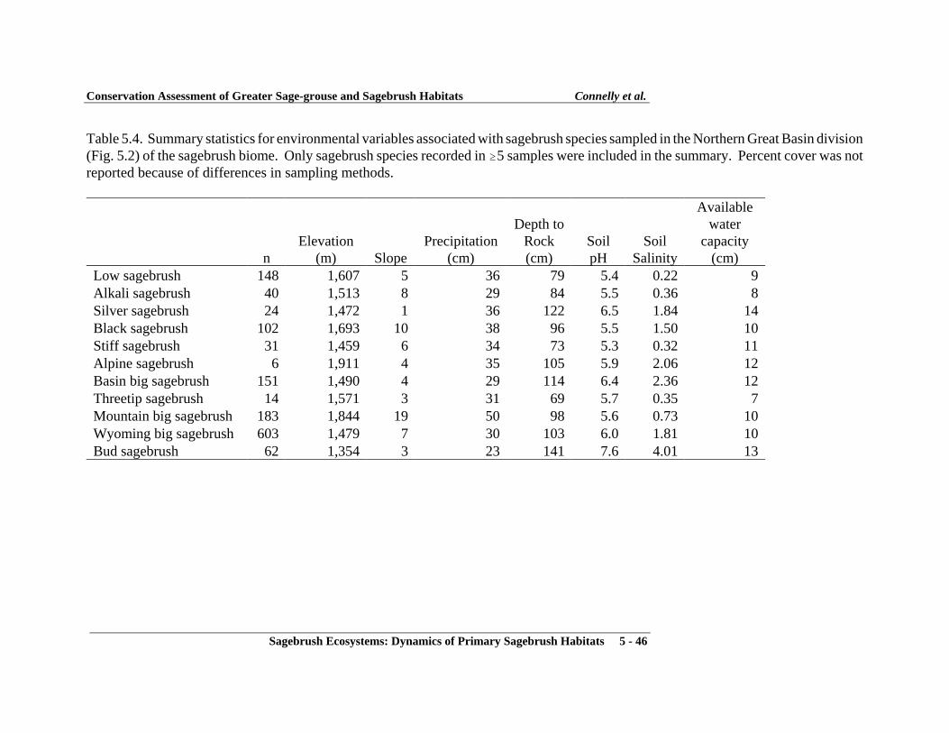
Conservation Assessment of Greater Sage-grouse and Sagebrush Habitats Connelly et al.
Sagebrush Ecosystems: Dynamics of Primary Sagebrush Habitats 5 - 46
Table 5.4. Summary statistics for environmental variables associated with sagebrush species sampled in the Northern Great Basin division(Fig. 5.2) of the sagebrush biome. Only sagebrush species recorded in $5 samples were included in the summary. Percent cover was notreported because of differences in sampling methods.
nElevation
(m) SlopePrecipitation
(cm)
Depth toRock(cm)
SoilpH
SoilSalinity
Availablewater
capacity(cm)
Low sagebrush 148 1,607 5 36 79 5.4 0.22 9Alkali sagebrush 40 1,513 8 29 84 5.5 0.36 8Silver sagebrush 24 1,472 1 36 122 6.5 1.84 14Black sagebrush 102 1,693 10 38 96 5.5 1.50 10Stiff sagebrush 31 1,459 6 34 73 5.3 0.32 11Alpine sagebrush 6 1,911 4 35 105 5.9 2.06 12Basin big sagebrush 151 1,490 4 29 114 6.4 2.36 12Threetip sagebrush 14 1,571 3 31 69 5.7 0.35 7Mountain big sagebrush 183 1,844 19 50 98 5.6 0.73 10Wyoming big sagebrush 603 1,479 7 30 103 6.0 1.81 10Bud sagebrush 62 1,354 3 23 141 7.6 4.01 13

Conservation Assessment of Greater Sage-grouse and Sagebrush Habitats Connelly et al.
Sagebrush Ecosystems: Dynamics of Primary Sagebrush Habitats 5 - 47
Table 5.5. Summary statistics for environmental variables associated with sagebrush species sampled in the Snake River Plain subdivision(Fig. 5.2) of the sagebrush biome. Only sagebrush species recorded in $5 samples were included in the summary. Percent cover was notreported because of differences in sampling methods.
nElevation
(m) SlopePrecipitation
(cm)
Depth toRock(cm)
SoilpH
SoilSalinity
Availablewater
capacity(cm)
Low sagebrush 314 1,903 11 43 108 6.4 0.95 10Alkali sagebrush 20 1,822 3 45 80 5.8 0.68 8Silver sagebrush 39 1,782 5 41 100 6.1 0.55 12Prairie sandwort 32 2,034 20 43 124 6.5 1.04 10Black sagebrush 161 1,799 9 37 124 7.1 2.01 10Stiff sagebrush 25 1,145 12 57 86 5.9 0.01 12Threetip sagebrush 178 1,711 8 42 121 6.6 0.72 18Basin big sagebrush 534 1,468 7 37 111 6.5 1.33 15Mountain big sagebrush 831 1,992 22 55 109 6.3 0.74 12Wyoming big sagebrush 1,140 1,533 8 33 112 6.4 1.55 12Bud sagebrush 11 1,217 1 24 130 7.2 3.76 16

Conservation Assessment of Greater Sage-grouse and Sagebrush Habitats Connelly et al.
Sagebrush Ecosystems: Dynamics of Primary Sagebrush Habitats 5 - 48
Table 5.6. Summary statistics for environmental variables associated with sagebrush species sampled in the Southern Great Basin division(Fig. 5.2) of the sagebrush biome. Only sagebrush species recorded in $5 samples were included in the summary. Percent cover was notreported because of differences in sampling methods.
nElevation
(m) SlopePrecipitation
(cm)
Depth toRock(cm)
SoilpH
SoilSalinity
Availablewater
capacity(cm)
Low sagebrush 378 2,165 16 41 92 6.1 0.98 8Alkalai sagebrush 68 1,929 12 32 103 6.0 1.31 8Bigelow sagebrush 7 1,782 8 22 78 6.0 3.96 9Silver sagebrush 46 2,484 11 64 120 6.4 1.07 14Black sagebrush 1,726 1,924 11 29 101 6.3 1.81 8Pygmy sagebrush 10 1,819 2 25 124 7.2 2.26 11Alpine sagebrush 7 3,126 28 85 89 5.1 -- 7Threetip sagebrush 13 2,025 14 42 98 6.0 1.35 10Subalpine sagebrush 129 1,784 15 24 89 6.2 1.65 7Basin big sagebrush 769 1,845 8 30 103 6.5 2.09 10Mountain big sagebrush 1,518 2,274 24 50 88 6.0 0.71 9Wyoming big sagebrush 2,521 1,832 7 29 120 6.7 2.33 11Bud sagebrush 790 1,567 3 20 134 7.4 4.03 11

Conservation Assessment of Greater Sage-grouse and Sagebrush Habitats Connelly et al.
Sagebrush Ecosystems: Dynamics of Primary Sagebrush Habitats 5 - 49
Table 5.7. Summary statistics for environmental variables associated with sagebrush species sampled in the Wyoming Basin division (Fig.5.2) of the sagebrush biome. Only sagebrush species recorded in $5 samples were included in the summary. Percent cover was notreported because of differences in sampling methods.
nElevation
(m) SlopePrecipitation
(cm)
Depth toRock(cm)
SoilpH
SoilSalinity
Availablewater
capacity(cm)
Low sagebrush 97 2,059 10 36 111 7.4 1.34 14Silver sagebrush 28 2,144 8 45 125 7.1 0.98 15Prairie sandwort 11 2,310 18 35 67 6.5 1.58 9Black sagebrush 147 1,976 13 30 75 6.7 1.42 10Basin big sagebrush 160 1,969 8 33 102 7.2 1.48 13Mountain big sagebrush 256 2,163 13 45 105 7.1 0.98 13Wyoming big sagebrush 419 1,976 7 32 104 7.1 1.54 14

Conservation Assessment of Greater Sage-grouse and Sagebrush Habitats Connelly et al.
Sagebrush Ecosystems: Dynamics of Primary Sagebrush Habitats 5 - 50
Table 5.8. Summary statistics for environmental variables associated with cheatgrass, and combined species of exotic grasses (includingcheatgrass) and native grasses sampled in the Colorado Plateau division (Fig. 5.2) of the sagebrush biome. Percent cover was not reportedbecause of differences in sampling methods.
nElevation
(m) SlopePrecipitation
(cm)
Depth toRock(cm)
SoilpH
SoilSalinity
Availablewater
capacity(cm)
Cheatgrass 78 1551 4 28 88 6.3 1.12 11Exotic grasses 92 1645 5 31 88 6.3 1.12 11Native grasses 198 1660 11 29 87 6.3 1.21 10
Table 5.9. Summary statistics for environmental variables associated with cheatgrass, and combined species of exotic grasses (includingcheatgrass) and native grasses sampled in the Columbia Basin division (Fig. 5.2) of the sagebrush biome. Percent cover was not reportedbecause of differences in sampling methods.
nElevation
(m) SlopePrecipitation
(cm)
Depth toRock(cm)
SoilpH
SoilSalinity
Availablewater
capacity(cm)
Cheatgrass 495 655 13 29 93 6.2 0.34 13Exotic grasses 577 667 13 30 95 6.2 0.32 13Native grasses 744 761 13 31 90 6.1 0.28 12

Conservation Assessment of Greater Sage-grouse and Sagebrush Habitats Connelly et al.
Sagebrush Ecosystems: Dynamics of Primary Sagebrush Habitats 5 - 51
Table 5.10. Summary statistics for environmental variables associated with cheatgrass, and combined species of exotic grasses (includingcheatgrass) and native grasses sampled in the Northern Great Basin division (Fig. 5.2) of the sagebrush biome. Percent cover was notreported because of differences in sampling methods.
nElevation
(m) SlopePrecipitation
(cm)
Depth toRock(cm)
SoilpH
SoilSalinity
Availablewater
capacity(cm)
Cheatgrass 705 1,456 10 30 111 6.4 2.52 11Exotic grasses 777 1,462 9 30 110 6.3 2.39 11Native grasses 923 1,591 8 35 99 5.8 1.45 10
Table 5.11. Summary statistics for environmental variables associated with cheatgrass, and combined species of exotic grasses (includingcheatgrass) and native grasses sampled in the Snake River division (Fig. 5.2) of the sagebrush biome. Percent cover was not reportedbecause of differences in sampling methods.
nElevation
(m) SlopePrecipitation
(cm)
Depth toRock(cm)
SoilpH
SoilSalinity
Availablewater
capacity(cm)
Cheatgrass 877 1379 10 34 106 6.4 1.55 13Exotic grasses 1,502 1504 10 38 111 6.5 1.46 13Native grasses 3,795 1787 13 45 111 6.3 1.15 12

Conservation Assessment of Greater Sage-grouse and Sagebrush Habitats Connelly et al.
Sagebrush Ecosystems: Dynamics of Primary Sagebrush Habitats 5 - 52
Table 5.12. Summary statistics for environmental variables associated with cheatgrass, and combined species of exotic grasses (includingcheatgrass) and native grasses sampled in the Southern Great Basin division (Fig. 5.2) of the sagebrush biome. Percent cover was notreported because of differences in sampling methods.
nElevation
(m) SlopePrecipitation
(cm)
Depth toRock(cm)
SoilpH
SoilSalinity
Availablewater
capacity(cm)
Cheatgrass 2,383 1,655 10 28 113 6.8 2.86 10Exotic grasses 3,057 1,744 11 32 113 6.7 2.59 11Native grasses 6,560 1,956 13 37 110 6.6 2.12 11
Table 5.13. Summary statistics for environmental variables associated with cheatgrass, and combined species of exotic grasses (includingcheatgrass) and native grasses sampled in the Wyoming Basin division (Fig. 5.2) of the sagebrush biome. Percent cover was not reportedbecause of differences in sampling methods.
nElevation
(m) SlopePrecipitation
(cm)
Depth toRock(cm)
SoilpH
SoilSalinity
Availablewater
capacity(cm)
Cheatgrass 172 1,843 9 27 88 6.6 1.89 11Exotic grasses 298 1,940 10 39 100 6.7 1.43 12Native grasses 1,099 2,093 12 44 103 6.9 1.23 13

Conservation Assessment of Greater Sage-grouse and Sagebrush Habitats Connelly et al.
Sagebrush Ecosystems: Dynamics of Primary Sagebrush Habitats 5 - 53
Table 5.14. Correlations of environmental variables with ordination axes (Fig. 5.6) using adetrended canonical correlation analysis of sagebrush communities and environmental variables.
Correlations of Environmental Variables with AxesVariable Axis 1 Axis 2
Elevation (m) -0.47 -0.37Slope -0.22 0.05Aspect -0.02 0.01Precipitation (cm) -0.46 0.02Depth to rock (cm_ 0.04 0.03Soil pH 0.08 0.01Soil Salinity 0.26 0.00Available water capacity (cm) 0.01 0.15

Conservation Assessment of Greater Sage-grouse and Sagebrush Habitats Connelly et al.
Sagebrush Ecosystems: Dynamics of Primary Sagebrush Habitats 5 - 54
Table 5.15. General structure and dominant species groups representing major existing post-settlement steady states, which occur across Artemisia plant associations.
Community Structure
Conifer
sp.
Artemisia
sp.
Native
Perennials
Introduced
Perennials Exoticsa
Shrublands
Shrub-steppe % % Shrublandb %
c
Shrub-exotic herblandb % %
Herblands
Exotic herbland
%
Perennial grassland %
Woodlands
Woodland native
understory
% %
Woodland % Woodland exotic
understoryb
% %
aExotics represent a range of annual, biennial, and perennial Eurasian and Mediterranean weedyspecies including cheatgrass, medusahead, knapweed sp., leafy spurge, and others.bSteady states that will probably shift to annual-biennial-perennial herbland following fire. cExotics often present but in low abundance

Conservation Assessment of Greater Sage-grouse and Sagebrush Habitats Connelly et al.
Sagebrush Ecosystems: Dynamics of Primary Sagebrush Habitats 5 - 55
Table 5.16. Percent of sagebrush in Küchler’s (1970) map of potential vegetation (Fig. 5.3)currently in sagebrush habitat. Only comparisons for Küchler’s categories of Great Basin sagebrush,sagebrush steppe, and wheatgrass-needlegrass shrubsteppe were used in this analysis. Remainingpercentage consisted of habitat categories describing barren, burn, grassland, exotic grassland, burn,nonsagebrush shrublands, and juniper woodland habitats.
Current Condition
State
Potential Area
(km2)
Sagebrush
km2 (%)
Agriculture
km2 (%)Washington 32,645 13,945 (42.7) 15,880 (48.6)Montanaa 9,321 3,953 (42.4) 585 (6.3)Wyoming 91,783 61,151 (66.6) 5,525 (6.0)Idaho 88,084 43,438 (49.3) 21,966 (24.9)Oregon 71,873 44,345 (61.7) 9,044 (12.6)Nevada 130,542 73,079 (56.0) 2,910 (2.2)Utah 30,976 11,253 (36.3) 4,105 (13.3)California 13,463 8,515 (63.2) 1,444 (10.7)Colorado 18,409 8,860 (48.1) 3,670 (19.9)Total 487,095 268,539 (55.1) 65,129 (13.3)
aSagebrush lands in eastern Montana outside the boundaries of the Küchler’s vegetation types usedin this analysis.

Conservation Assessment of Greater Sage-grouse and Sagebrush Habitats Connelly et al.
Sagebrush Ecosystems: Dynamics of Primary Sagebrush Habitats 5 - 56
Table 5.17. Characteristics of lands within the sagebrush biome under different management authority and ownership status. Wedetermined characteristics for lands managed by the U.S. Bureau of Land Management (BLM), U.S.D.A. Forest Service (USFS), andcombined totals for individual state agencies. Fragmentation was the number of edges in the gridded map (Fig. 5.16) between sagebrushand other habitats in the landscape within a 5- and 18-km radius.
Stewardship
Sagebrush
Cover
(% 5-km)a
Sagebrush
Cover
(% 18-km)a
Precipitation
(cm)
Elevation
(m) Salinity
Soil
pH
Available
Water
Capacity
(cm)
Soil
Depth
(cm)
Fragmentation
(5-km)
Fragmentation
(18-km)Private 16 16 39 1,356 1.92 6.7 15 114 87 263BLM 41 39 30 1,694 2.24 6.4 10 99 101 321USFS 10 12 75 2,169 0.46 5.3 11 104 100 290State Agency 18 17 39 1,551 1.93 6.6 13 109 104 315BLM / USFS 7 10 64 2,462 0.48 4.8 8 84 54 163Other 15 15 38 1,478 2.10 5.9 11 94 79 230aDetermined from GIS coverage of % cover of sagebrush within 5-km radius (Fig. 5.14)

Chapter 6
Greater Sage-Grouse Populations

Greater Sage-Grouse Populations 6 - 1
CHAPTER 6
Greater Sage-Grouse Populations
Abstract. This chapter presents information on three different but related subjects. 1) State and province sage-grouse population databases. To obtain information on the scope and extent of population databases we mailed a detailed questionnaire to 11 western states and 2 Canadian provinces. We requested information on methods used for monitoring sage-grouse (Centrocercus urophasianus and C. minimus) populations, production, and harvest, as well as information on data storage and data retrieval. Results from our questionnaire indicated monitoring techniques vary among areas and years both within and among agencies. This variation complicates attempts to understand grouse population trends and make comparisons among areas. Moreover, there were discrepancies between information reported by agencies in the questionnaire and that obtained from the agencies’ lek databases. 2) Sage-grouse distribution. We presented information on the range-wide distribution of sage grouse. The overall distribution of potential pre-settlement habitat was estimated to have been 1,200,483 km2 and the current distribution to be 668,412 km2. Approximately 56% of the potential pre-settlement distribution of habitat is currently occupied. Future examinations of regional habitat and habitat change should provide more insight into long-term changes in the distribution of sage-grouse. The area currently occupied by sage-grouse is clearly smaller than was occupied in pre-settlement times. Declines in distribution have been noted throughout the twentieth century. 3) Sage-grouse population trends. We conducted a comprehensive analysis of sage-grouse population changes throughout their range by accumulating and analyzing all available male counts at 5,585 leks identified since agencies began routine monitoring of this species. A substantial number of lek routes and leks are censused each year throughout North America and many of these databases have > 30 years of information. We discuss problems associated with the collection and analysis of these data sets but they represent the only long-term database available for sage-grouse. Virtually all states and provinces have increased monitoring efforts, especially over the last 10 years. Our analysis indicated that a total of 2,637 leks are now censused annually. We used three different but related methods to assess population trend. Eleven of 13 (85%) states and provinces showed significant long-term declines in size of active leks. Similarly, eight of 10 states (80%) showed population declines over that time frame. Two of 10 (20%) appeared to be stable or slightly increasing. Only California had an increase in both the population index and lek size. Annual rates of change suggest a long-term decline for sage-grouse in western North America and generally support the trend information obtained from lek attendance (males/lek). Range-wide sage-grouse populations declined at an overall rate of 2.0% per year from 1965 to 2003. This annual rate of decline was much higher during the first two decades of our analysis period (1965-86) compared to the last two decades (1986-2003). Although a total of 50,566 male sage-grouse were counted on leks in 2003 throughout western North America, long-term population changes coupled with continued loss and degradation of habitat and other factors (including West Nile Virus) do not provide causes for optimism.
POPULATION DATABASES
Introduction
Greater sage-grouse populations have been declining for at least 25 years (Braun 1995, Connelly and Braun 1997, Aldridge and Brigham 2003, Beck et al. 2003, Schroeder et al. 2004). Because of concerns about this species and its habitats, appropriate monitoring efforts have become more important. Connelly et al. (2000) indicated that monitoring was a major component of a sage-grouse management program. Additionally, representatives to the Western Association of Fish and Wildlife Agencies (WAFWA) signed memorandum of agreements among themselves (1999) and with federal agencies (2001) to collect data in a manner recommended by the Western States Sage and Columbian Sharp-tailed grouse Technical Committee.

Conservation Assessment of Greater Sage-grouse and Sagebrush Habitats Connelly et al.
Greater Sage-Grouse Population 6 - 2
As part of the Conservation Assessment for greater sage-grouse, we attempted to obtain information on current sage-grouse monitoring programs by mailing a questionnaire to all state and provincial agencies (n = 13) that manage this species. Here we summarize the responses to this questionnaire and identify strengths and weaknesses of current data sets.
Methods
We mailed a detailed questionnaire to 11 western states and 2 Canadian provinces. This questionnaire requested information on methods used for monitoring sage-grouse breeding populations, production, and harvest. We also requested information on data storage and retrieval. To aid biologists responding to this questionnaire, we provided the following definitions:
Lek—a traditional display area where > 2 male grouse have attended in > 2 of the previous five years. Lek count—a tally of male sage-grouse on a lek or group of leks with no assumption that the leks represent all or part of a single breeding population. Lek route—A count of male sage-grouse on a group of leks that are relatively close and represent all or part of a single breeding population. Lek survey—A classification of leks as active or inactive, often done from an aircraft.
All states and provinces returned completed questionnaires. Because no respondents
indicated those questions were difficult to understand or ambiguous, we did not follow up with additional questions or phone calls. Data reported in this section refer to only information obtained from the questionnaires and not to databases subsequently obtained from states and provinces.
Results Population Data
All state and provincial fish and wildlife agencies monitor sage-grouse breeding
populations annually, but different approaches are employed (Table 6.1). Five agencies use only lek counts. Eight use a combination of techniques: three agencies use lek counts and lek routes; one agency uses lek counts and lek surveys; four agencies use lek counts, lek routes, and lek surveys.
Responses from agencies indicated that a total of 237 lek routes and 2,046 leks are censused throughout North America (Table 6.1). Within the same area, 2,304 leks were surveyed. Montana, Wyoming, and Idaho count the greatest number of leks (498, 375, 352, respectively). Actual values from state databases are presented later in this chapter.
Twelve agencies indicated that their monitoring data were widely distributed across the
range of the species within their state or province. Ten agencies (77%) reported starting

Conservation Assessment of Greater Sage-grouse and Sagebrush Habitats Connelly et al.
Greater Sage-Grouse Population 6 - 3
monitoring programs in the 1940s or 1950s. Two (15%) started programs in the 1960s or 1970s, and one agency started monitoring in the 1990s (Table 6.1). Of the 12 agencies responding, 11 indicated that population data were obtained over multiple administrative units (range = 2-35, x = 10). These administrative units were counties, agency-delineated regions, or hunting units. Table 6.1. Year monitoring started, number of lek routes run, and leks counted or surveyed in western states and provinces, 2002.1 State/Province Year Started Number of Routes Leks Counted Leks Surveyed Alberta 1968 0 32 27 California 1953 3 64 100 Colorado 1959 0 278 0 Idaho 1951 51 352 273 Montana 1950s 4 498 0 North Dakota 1951 0 17 25 Nevada 1950s 4 110 994 Oregon 1947 39 124 46 Saskatchewan 1994 0 35 0 South Dakota 1972 0 20 0 Utah 1959 0 170 0 Washington 1954 0 20 0 Wyoming 1949 139 375 831 Totals 240 2,095 2,296
1These data were reported by the agencies and do not necessarily reflect information obtained from the agencies’ databases for the conservation assessment.
Although most agencies indicated that they attempted to replicate counts of leks over
several weeks (i.e., counting individual leks or lek routes >3 times), at least 2 agencies attempt to complete all counts within a 1-week period and one only counts leks once during this time. In addition, some states provided data indicating leks were censused at inappropriate times (late February, early to mid-March, mid-May). Eight (62%) agencies indicated gaps in their databases since initiating monitoring efforts and five (38%) reported relatively continuous databases. Eleven of 13 (85%) agencies reported changing inventory methods over the years. Harvest Data
Ten of 11 states have hunting seasons. Sage-grouse are not hunted in Washington,
Alberta and Saskatchewan. All states with a hunting season collected wings (Table 6.2). Three states collected >1000 wings each year, 5 states collected 200-600 wings each year and 2 states collected < 50 wings per year. The number of administrative units that each state used for data analysis varied greatly among states (Table 6.2) and seven states analyzed data by administrative
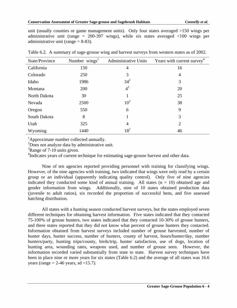
Conservation Assessment of Greater Sage-grouse and Sagebrush Habitats Connelly et al.
Greater Sage-Grouse Population 6 - 4
unit (usually counties or game management units). Only four states averaged >150 wings per administrative unit (range = 200-397 wings), while six states averaged <100 wings per administrative unit (range = 8-83). Table 6.2. A summary of sage-grouse wing and harvest surveys from western states as of 2002. State/Province Number wings1 Administrative Units Years with current survey4
California 150 4 16 Colorado 250 3 4 Idaho 1986 342 3 Montana 200 42 20 North Dakota 30 1 25 Nevada 2500 103 38 Oregon 550 6 9 South Dakota 8 1 3 Utah 325 4 2 Wyoming 1440 182 46 1Approximate number collected annually. 2Does not analyze data by administrative unit. 3Range of 7-10 units given. 4Indicates years of current technique for estimating sage-grouse harvest and other data.
Nine of ten agencies reported providing personnel with training for classifying wings.
However, of the nine agencies with training, two indicated that wings were only read by a certain group or an individual (apparently indicating quality control). Only five of nine agencies indicated they conducted some kind of annual training. All states (n = 10) obtained age and gender information from wings. Additionally, nine of 10 states obtained production data (juvenile to adult ratios), six recorded the proportion of successful hens, and five assessed hatching distribution.
All states with a hunting season conducted harvest surveys, but the states employed seven different techniques for obtaining harvest information. Five states indicated that they contacted 75-100% of grouse hunters, two states indicated that they contacted 10-30% of grouse hunters, and three states reported that they did not know what percent of grouse hunters they contacted. Information obtained from harvest surveys included number of grouse harvested, number of hunter days, hunter success, number of hunters, county of harvest, hours/hunter/day, number hunters/party, hunting trips/county, birds/trip, hunter satisfaction, use of dogs, location of hunting area, wounding rates, weapons used, and number of grouse seen. However, the information recorded varied substantially from state to state. Harvest survey techniques have been in place nine or more years for six states (Table 6.2) and the average of all states was 16.6 years (range = 2-46 years, sd =15.7).

Conservation Assessment of Greater Sage-grouse and Sagebrush Habitats Connelly et al.
Greater Sage-Grouse Population 6 - 5
Production Data Only Oregon and California reported conducting routine production surveys in addition
to collecting wings. California indicated that they conducted production surveys in some areas to monitor for “abnormalities” and track key brood rearing areas. None of the agencies that did not have hunting seasons routinely monitored production. Thus, 10 of 11 agencies assessed production with wing collections and in two cases also with brood counts. Data Storage and Retrieval
Nine of 13 (69%) agencies stored their data in two or more formats. Five of 13 (38%)
indicated that at least some of their data were stored on paper (i.e., information was not in a database or spreadsheet program). Only four of 13 (31%) agencies reported that their data were stored in a single format (e.g., Excel).
Seven of nine agencies reported that they could transmit data to the Conservation
Assessment Team in two weeks or less. Unfortunately, four agencies indicated it would take 2-6 months and one of these said that it could take up to a year. Montana did not provide an estimate.
Eight of 13 agencies (62%) rated their monitoring data as good; an additional state
indicated that some of their data were good. Four of 13 (31%) indicated that their monitoring data was fair and one state reported that about 60% of their data was fair or poor. Of these five states, four (ID, OR, CO and NV) have long histories of sage-grouse work and all four started breeding population data collection in the 1940s or 1950s.
Discussion
Sage-grouse populations in parts of western North America have been monitored in some fashion for over 50 years (Patterson 1952, Dalke et al. 1963). In a non peer-reviewed report, Autenrieth et al. (1982) recognized the variation in monitoring efforts among agencies. In an attempt to improve data collection, the Western States Sage Grouse Committee (now the Western States Sage and Columbian Sharp-tailed Grouse Technical Committee) issued a bulletin on sage-grouse management practices (Autenrieth et al. 1982). This report, in part, attempted to standardize population data collection techniques and describe methods available for documenting sage-grouse population characteristics. However, results from our questionnaire indicated monitoring techniques continue to vary among areas and years both within and among agencies. This variation complicates attempts to understand grouse population trends and make comparisons among areas. Moreover, there were many discrepancies between information reported by agencies in the questionnaire and that obtained from the agencies’ lek databases. This suggests that until very recently many agencies did not have a clear understanding of their data or methods for collecting it. Clearly, this assessment has resulted in most agencies closely examining their sage-grouse monitoring program. The sage-grouse guidelines (Connelly et al. 2000) stressed the importance of population monitoring and collecting quality data in sage-grouse management programs. Information from the questionnaire suggests some recent effort among agencies to improve or update data collection efforts.

Conservation Assessment of Greater Sage-grouse and Sagebrush Habitats Connelly et al.
Greater Sage-Grouse Population 6 - 6
Population Data
Although lek counts are widely used, a non-peer reviewed report (Beck and Braun 1980) for the Western Association of Fish and Wildlife Agencies questioned their usefulness. However, techniques for correctly conducting lek counts have been described (Jenni and Hartzler 1978, Emmons and Braun 1984) and problems generally seem to be related to disregarding accepted techniques. We did not question agencies about lek counting procedures because lek data submitted by states and provinces provided insight into methods used. It was clear that some agencies attempted to follow accepted techniques while others developed their own approach. An evaluation of lek data indicated that some leks were counted incorrectly, because observers collected data too early or late in the breeding season, in poor weather and/or later in the morning.
Because sage-grouse gather on traditional display areas (leks) each spring, biologists are
afforded relatively easy methods for tracking breeding populations (Connelly et al. 2003). These methods have included lek censuses (annually counting the number of male sage-grouse attending leks in a given area), lek routes (annually counting the number of male sage-grouse on a group of leks that are relatively close and represent part or all of a single breeding population or deme), and lek surveys (annually counting the number of active leks in a given area). All lek monitoring procedures are supposed to be conducted during early morning (1/2 hour before to 1 hour after sunrise), with reasonably good weather (light or no wind, partly cloudy to clear) from early March to early May (Connelly et al. 2003). Timing of lek monitoring is dependent on elevation of leks and persistence of winter conditions. Sage-grouse will begin displaying in late February at lower elevations with milder climates and in years with mild winter weather (e.g., southern Washington). Lek attendance will persist into early or mid-May at higher elevations.
A substantial number of lek routes and leks are censused each year throughout North
America and many of these databases have > 30 years of information. Virtually all agencies report monitoring sage-grouse throughout much of the species’ range within their respective state or province. However, methods for gathering these data vary widely among agencies and sometimes within agencies among years.
Responses to the questionnaire suggested that the same leks or leks within the same area,
have been counted for long periods of time. These leks were likely originally selected because of size (leks with many males), access, or both reasons. In any case, leks that are censused in most states and provinces are probably not a random sample of available leks and thus data obtained from these leks may be biased (but see Appendix 3). However, some states and provinces attempt to monitor all of their leks.
Lek counts focus on attendance of males. Male sage-grouse sometimes do not attend a
lek or may attend two or more different leks (Jenni and Hartzler 1978, Walsh 2002). Lek data used to track population trends have an implied assumption that the probability of detection of birds does not change among years (i.e., the proportion missed because of non-attendance or attendance at a lek that is not counted remains about the same). Even if the detection probability is unknown (almost always the case), the problem can be somewhat minimized, and thus provide more precise counts, if leks counted on a single morning are relatively close and represent all or
Conservation Assessment of Greater Sage-grouse and Sagebrush Habitats Connelly et al.
Greater Sage-Grouse Population 6 - 7
a significant part of a given breeding population. Thus lek routes are preferable to lek counts because they should increase the probability of detection of male grouse (i.e., if a male grouse normally is counted on lek “A” but spends 20% of his time on lek “B” and both leks are counted on the same morning, the probability of detecting that bird is greater than if just lek “A” were counted). Harvest Data
Although numerous wings are collected in many states and the wings subsequently classified in “wing-bees”, numbers may be insufficient to characterize populations, depending on the number of administrative units used for analysis. In a non-peer-reviewed report, the Western States Sage and Columbian Sharp-tailed Grouse Technical Committee (Autenrieth et al. 1982) suggested that at least 100 wings from adult and yearling hens are needed from each population to obtain meaningful data. Questionnaire responses suggest six of 10 states have less than 100 wings per administrative unit. Thus, at least 60% of states likely do not obtain adequate samples of wings to assess production. Moreover, these wings represent both genders and age groups, further indicating that sample size is quite low. Additionally, because grouse are often hunted on summer ranges and birds from two or more breeding populations may use the same summer ranges (Connelly et al. 1988, Wakkinen 1990, Fischer 1994, Wik 2002), production data may be difficult to interpret. Collection techniques currently do not appear designed to reflect known breeding populations. Because of low sample sizes, lack of wings in some states and provinces, and an inability to relate wing surveys to breeding populations we did not use wing data to help assess sage-grouse population trends.
Training or other quality control practices are used in most states but only five of nine
states indicated annual training for wing-bee participants. One state indicated that each participant was tested before beginning to read wings. Where participants remain the same each year, frequent training may not be necessary.
All states with hunting seasons monitor sage-grouse harvest. However there seems to be a great deal of uncertainty associated with harvest estimates. Seven different techniques are used among the 10 agencies that administer hunting seasons and a variety of information is obtained from these techniques. This information varies tremendously among states. Production Data
Brood routes are not a commonly used technique for monitoring production. Oregon uses these data in conjunction with breeding population data to develop hunting seasons (W. Van Dyke, Oregon Department of Fish and Wildlife, personal communication) and apparently is the only state to use these data for this purpose. The state and provinces without hunting seasons do not use brood routes and thus have no means of assessing production, except by using studies involving radio telemetry.
Data Storage and Retrieval
Agencies not only vary greatly in how they collect data but also how they manage databases. However, most agencies indicated that they could compile and transmit their data

Conservation Assessment of Greater Sage-grouse and Sagebrush Habitats Connelly et al.
Greater Sage-Grouse Population 6 - 8
rather quickly. Interestingly, 62% of the agencies had a similar view of their data by rating it as good. Agencies that took a more critical view of their data sets were involved with long-term monitoring and research programs on sage-grouse. This emphasis may have provided these agencies with a better understanding of the quality and quantity of their data compared to agencies whose sage-grouse management program is only comprised of monitoring.
DISTRIBUTION
The general distribution of sage-grouse is clearly associated with distribution of sagebrush (Artemisia spp.), in particular, big sagebrush (A. tridentata), but also silver sagebrush (A. cana). This relationship has been illustrated in numerous descriptions or maps of the sage-grouse distribution (summarized in Schroeder et al. 2004). Schroeder et al. (2004) revised the current and pre-settlement (past, original, or historical) sage-grouse map with numerous sources of information including: 1) past maps showing distribution of sage-grouse (e.g. Aldrich and Duvall 1955); 2) maps and research on the distribution of habitat types in western North America (e.g. Kuchler 1985); 3) recovery locations for 1,167 sage-grouse museum specimens (Schroeder et al. 2004); 4) published sage-grouse observations, many from the 1800s (Schroeder et al. 2004); 5) known information on current and past occurrence of sage-grouse, such as lek locations; and 6) research elucidating the movement (Connelly et al. 1988) and habitat use (Schroeder et al. 1999, Connelly et al. 2000) of sage-grouse. ‘Pre-settlement’ was used to define the period prior to 1800 before rapid settlement by people of European descent, particularly in Nevada, Oregon, and Utah (Miller and Eddleman 2001).
Seven core habitats from Kuchler’s (1985) map were used to help define the pre-
settlement distribution (see Chapter 5, Fig. 5.3). The seven core habitats that supported the most sage-grouse included: 1) sagebrush steppe, 2) Great Basin sagebrush, 3) wheatgrass (Agropyron spicatum)-needlegrass (Stipa spp.) shrubsteppe, 4) grama (Bouteloua spp.)-needlegrass-wheatgrass, 5) wheatgrass-needlegrass, 6) wheatgrass-bluegrass (Poa spp.), and 7) fescue (Festuca spp.)-wheatgrass. Although Kuchler’s habitat map indicates some of these core habitats are not dominated by sagebrush, a key component of sage-grouse habitat, data from portions of these regions (e.g., Daubenmire 1970, Brown and Lowe 1980, Jacobson and Snyder 2000) indicates that sagebrush may be locally abundant within definable portions of an otherwise grass-dominated habitat type. Consequently, only sagebrush-dominated portions of three core habitat types (wheatgrass-needlegrass, wheatgrass-bluegrass, fescue-wheatgrass) were mapped as part of the pre-settlement distribution of potential sage-grouse habitat. Comparison of Kuchler’s (1985) map with known information on sage-grouse abundance and habitat use illustrated the existence of several ‘secondary’ habitats. Secondary habitats are characterized by variation in suitability due to tree abundance, sagebrush type and density, and connectivity and proximity to core habitats (Connelly et al. 2000, Miller and Eddleman 2001). Secondary habitats include: 1) foothills prairie, 2) saltbush (Atriplex spp.)-greasewood (Sarcobatus vermiculatus), 3) juniper (Juniperus spp.)-pinyon (Pinus edulis) woodland, 4) grama-buffalo grass (Buchloe dactyloides), and 5) desert. Secondary habitats were mapped locally in specific situations where the habitats: 1) are currently occupied, 2) were clearly occupied in the past, and 3) are generally within 10 km of core habitats. Habitats without known use by sage-grouse were excluded from the pre-settlement distribution of potential habitat, even if there were scattered observations and/or recoveries of sage-grouse.

Conservation Assessment of Greater Sage-grouse and Sagebrush Habitats Connelly et al.
Greater Sage-Grouse Population 6 - 9
The map revisions were designed to result in the following improvements: 1) mapping at
larger scale to improve precision with respect to topography and habitat types (1:2,000,000); 2) placement in Geographical Information System (Arc/INFO 1998) to permit additional analysis (Wisdom et al. 2002a, b); 3) elimination of habitat that was clearly unsuitable (e.g., forest); 4) inclusion of suitable, or potentially suitable, habitat that had been excluded from earlier maps; and 5) integration of a map with at least 30 years of lek surveys throughout the range.
The descriptions of the sage-grouse distribution have been divided into general regions similar to those described by Miller and Eddleman (2001). These include the Wyoming Basin (W two-thirds of Wyoming, NE Utah, SE tip of Idaho, NW Colorado, SW Montana), Snake River Plain (S Idaho, NW Utah, NE Nevada, E Oregon), Columbia Basin (north-central Oregon, E Washington, south-central British Columbia), northern Great Basin (south-central Oregon, NE California, NW Nevada), southern Great Basin (east-central California, S two-thirds of Nevada, W and central Utah), and Colorado Plateau (only the NW Arizona and southern Utah). The Great Plains or silver sagebrush region (E and S Montana, W North Dakota, W South Dakota, NW Nebraska, E Wyoming, SW Saskatchewan, SE Alberta) has been added to include areas outside the scope of Miller and Eddleman’s (2001) map (Figure 1.5). Although the sage-grouse maps originally included the Gunnison (C. minimus) and greater species (Schroeder et al. 2004), only the greater sage-grouse is described in detail here.
General The overall distribution of potential pre-settlement habitat was estimated to have been
1,200,483 km2 and the current distribution to be 668,412 km2 (Chapter 1, Fig. 1.1) (Schroeder et al. 2004). Approximately 56% of the potential pre-settlement distribution of habitat is currently occupied. Specimens from Washington and Oregon were believed to be the western subspecies, specimens from California were believed to be an intermediate form, and all other specimens were believed to be the eastern subspecies (Aldrich and Duvall 1955). However, we made no attempt to quantify the respective distributions of the eastern and western subspecies (C. u. urophasianus and C. u. phaios, Aldrich 1946) because of the lack of a clear dividing line (Aldrich and Duvall 1955) and the lack of genetic differentiation (Chapter 8, Benedict et al. 2003). Great Plains
Members of the Lewis and Clark expedition observed sage-grouse in western Montana,
but not in central and eastern Montana (Zwickel and Schroeder 2003). Swainson and Richardson (1831:359) reported that sage-grouse “do not exist on the banks of the river Missouri; nor have they been seen in any place east of the Rocky Mountains.” Audubon mentioned that sage-grouse were observed by a member of his expedition prior to 1843 at some point on the Yellowstone River, however Audubon himself did not observe sage-grouse along the Missouri (Audubon 1960). Coues (1874) was the first to mention sage-grouse in central Montana. In contrast to earlier accounts, Bendire (1892) suggested the area of sage-grouse occupation included most of Montana and western North Dakota, stretching about 50 km north of the U.S.-Canadian border along the upper tributaries of the Missouri River. An examination of museum specimens and

Conservation Assessment of Greater Sage-grouse and Sagebrush Habitats Connelly et al.
Greater Sage-Grouse Population 6 - 10
published observations supports the past occurrence of sage-grouse up to 240 km north of the U.S.-Canadian border, however specimens and observations more than 100 km north of the border are all more recent than 1945 (Schroeder et al. 2004).
In his “List of Birds observed at Grand River Agency, Dakota Territory, from October 7, 1872 to June 7, 1873, W.J. Hoffman M.D., the Acting Assistant Surgeon for the U.S. Army stationed near the confluence of the Missouri and Grand Rivers in Dakota Territory reported that the “Sage Cock” Centrocercus urophasianus was not often found near the Agency but were often brought into the agency by the Indians “who shot them on the plains where artemisia occurs.” A 1914 report by Stephen S. Visher, published in Bulletin Number 6 of the South Dakota Geological Survey details the Biology of Harding County Northwestern South Dakota at that time. Visher indicated that sage-grouse “were formerly found in many sections of Western South Dakota and westward.” Visher further stated in his report that the sage hen was an:
“abundant resident in the areas covered with scrub-bush (Artemisia tridentata), where water is far distant; therefore mainly found on the terraces in the stream valleys. The last ones recorded from this state, except in the northwestern corner, were found in Sage Creek in the Badlands in 1907. By 1910 all were gone except those in Harding and Butte Counties. Now, (1913) after three more years of homesteading Sage Grouse are restricted in this state to the Little Missouri Valley in Harding County and to the headwaters of Indian Creek in Butte. In a very few years they will occur in South Dakota only as a rare winter straggler from Montana.” This information is contained in the South Dakota Geological Survey; Bulletin Number Six; Report of State Geologist; State Publishing Co., Pierre, SD and was provided to us by John Wrede (South Dakota Game, Fish and Parks). The dates and locations of observations between 1805 (Meriwether Lewis in Moulton
1987) and the mid-1900s support the possibility of a northward transition in distribution. However, there are limited data regarding the pre-settlement distribution of sagebrush throughout the region and regional variation in the density of ungulates (Martin and Szuter 1999, Lyman and Wolverton 2002). Additionally, sage-grouse are known to use alternate species of sagebrush such as silver sagebrush in Alberta, Saskatchewan, North Dakota, and South Dakota (Sealy 1963; Aldridge and Brigham 2002, 2003; Smith 2003). The lack of solid data on the presence of sage-grouse in most areas precluded attempts to divide the distribution into ‘originally occupied’ and ‘acquired’ portions. As a result, most observations and specimens within Alberta and Saskatchewan are included in the potential pre-settlement distribution of habitat (Schroeder et al. 2004).
Most museum specimens and early observations of sage-grouse in North and South Dakota are from an area that is either currently occupied or close to an area that is occupied (Schroeder et al. 2004). The absence of sage-grouse in most of North and South Dakota is further supported in a review by Johnson and Knue (1989) where they report the absence of sage-grouse remains at 27 of 29 Indian villages where sharp-tailed grouse (Tympanuchus phasianellus) remains were found. Consequently, the potential pre-settlement distribution of habitat was delineated to be consistent with most specimens and observations. The revised

Conservation Assessment of Greater Sage-grouse and Sagebrush Habitats Connelly et al.
Greater Sage-Grouse Population 6 - 11
distribution of habitat includes southwestern North Dakota, western South Dakota (except for forested portions of the Black Hills), and northwestern Nebraska, and does not extend into central North Dakota as shown by Aldrich and Duvall (1955).
Wyoming Basin Most early observations in this region were in south-central or southwestern Wyoming,
due in part to the location of a prominent travel corridor over South Pass (Stansbury 1852, Frémont 1887, Thwaites 1978). Field (1857) stated that sage-grouse were supported by vast expanses of sagebrush, particularly in southwestern Wyoming. Although there are no published early observations of sage-grouse in eastern portions of their current distribution in this region, it is not clear if this represents a shift in distribution or a bias related to their abundance in different areas and habitats. Aldrich and Duvall (1955) illustrated both current and past distribution of sage-grouse as being relatively continuous in most of the Wyoming Basin, with a general absence in the Grand Tetons, Yellowstone, and Wind River Mountain areas of Wyoming. However, sage-grouse currently occur around Jackson, Wyoming. The distribution of forested and alpine habitats also indicates that greater sage-grouse were likely absent from portions of the Big Horn Mountains and Black Hills in Wyoming, Uinta and Wasatch mountains in Utah, and Uncompahgre Plateau, Gore Range, and Flat Top Mountains in Colorado (Rogers 1964, Braun 1995). More than 6,000 birds were captured in Wyoming between 1940 and 1951 and moved to other areas in Wyoming with existing populations, but some were released in New Mexico within the former range of the Gunnison sage-grouse (Patterson 1952). Snake River Plain
The area on both sides of the continental divide near Lemhi Pass has been occupied by
sage-grouse for at least the last 200 years (Zwickel and Schroeder 2003). Aldrich and Duvall (1955) also showed an area of historical occupation by greater sage-grouse along the Bitterroot Valley in northwestern Montana; Aldrich’s revised map in 1963 did not include this area. One specimen apparently was collected near Missoula in 1900 (Schroeder et al. 2004). This area generally corresponds with the foothills prairie habitat (Kuchler 1985) that is occasionally occupied by sage-grouse in other portions of Montana. In 1942, 242 birds were captured in Montana and released in several locations including the Bitterroot Valley, an effort that was ultimately unsuccessful in establishing (or re-establishing) a population (Reese and Connelly 1997).
Current populations in the region occupy substantial areas of habitat that appear continuous across multi-state borders. The largest of these occupies the tri-state area of Idaho, Nevada, and Oregon, but smaller populations appear to cross other borders. Most of the fragmentation in populations is associated with the extirpations along the Snake River and its tributaries. In 1986, 196 sage-grouse were captured in Idaho and translocated to the Sawtooth Valley in an attempt to augment an isolated population that had declined to one displaying male. Although the ultimate fate of this translocation effort is unclear (Musil et al. 1993), population data suggests that it might be extirpated (Appendix 4, Figure A4.26).

Conservation Assessment of Greater Sage-grouse and Sagebrush Habitats Connelly et al.
Greater Sage-Grouse Population 6 - 12
Most areas close to the Snake River, which are almost completely unoccupied at present, likely supported sage-grouse in the past (Bean 1941). Observations of habitat along the Snake River Valley during the mid-1800s indicated that many of the well-traveled areas close to the river were dominated by sagebrush and little grass (Vale 1975). In addition, these areas are the lowest elevation and driest, and the most likely to be developed and/or converted (Bunting et al. 2002). It is possible that areas along the Snake River may have supported wintering sage-grouse when higher elevation habitats were covered with deep snow. Nevertheless, most museum specimens were collected at least 25 km from the Snake River, except for 3 specimens west of American Falls and another near Wilder, all collected in 1933 or earlier (Schroeder et al. 2004). This suggests that sage-grouse were extirpated close to portions of the Snake River relatively early, perhaps prior to 1900 in most cases. In addition, populations of sage-grouse are apparently continuing to recede from the Snake River and its tributaries, indicating this may be a long-term trend. Columbia Basin
Available evidence indicates that potential sage-grouse habitat once covered much of north-central Oregon, central and eastern Washington, and extended northward along the Okanogan River into southern British Columbia. Lewis and Clark noted sage-grouse on the plains between the confluence of the Columbia and Snake rivers (near present city of Kennewick, Washington) and the confluence of the Columbia and Deschutes rivers (Zwickel and Schroeder et al. 2003). David Douglas (Royal Historical Society 1914) observed sage-grouse near Wallula in 1826, and extremely large numbers of birds along the Columbia River near Priest Rapids, Washington (now under Priest Rapids Lake). The first record for sage-grouse in British Columbia was in 1864 near Osoyoos Lake; most subsequent records were in the same area (Campbell et al. 1989).
Jewett et al. (1953) and Aldrich and Duvall (1955) showed the past distribution of sage-
grouse straddling the border of Idaho and Washington on the eastern edge of the Palouse Prairie. However, because the potential pre-settlement habitat of the Palouse Prairie was likely dominated by perennial grasses with little sagebrush (Daubenmire 1970, Kuchler 1985) and because there are no observations or museum specimens in these portions of Idaho and Washington (Yocom 1956, Schroeder et al. 2000), the revised map of potential pre-settlement habitat does not include this area. Potential pre-settlement habitat in Washington was probably continuous with north-central Oregon (Schroeder et al. 2004). The continuity of these populations is one reason why the U.S. Fish and Wildlife Service considered the Oregon-Washington area to be a ‘distinct population segment’ (Warren 2001). Despite this apparent continuity, most of the early observations in the region are from the area near the confluence of the Snake and Columbia rivers (Peale 1848, Cassin 1978) with few observations in north-central Oregon (Schroeder et al. 2004).
Reductions in the distribution of sage-grouse in the region were noted as early as 1920 (Jewett et al. 1953). These reductions have been monitored to the present, with the declines continuing (Schroeder et al. 2000). Sage-grouse are almost completely extirpated from Washington, British Columbia, and northern Oregon. The last observation (prior to translocation efforts) in British Columbia was in 1918 near Oliver (Campbell et al. 1989). Although 57 birds

Conservation Assessment of Greater Sage-grouse and Sagebrush Habitats Connelly et al.
Greater Sage-Grouse Population 6 - 13
were translocated from the Malheur County, Oregon area to the Richter Lake area of British Columbia in 1958, the translocation was unsuccessful, with the last observation of birds in 1966 (Campbell et al. 1989). Between 1941 and 1951 there were efforts to re-establish or augment populations in Sherman and Umatilla counties in northern Oregon with birds captured in other areas of Oregon, however these translocations were also unsuccessful (Reese and Connelly 1997).
Northern Great Basin The potential pre-settlement distribution of habitat in this region is believed to encompass
substantial portions of south-central Oregon, northeastern California, and northwestern Nevada (Schroeder et al. 2004). The distribution of museum specimens and published observations appears to approximate the distribution of potential pre-settlement habitat for this area. Although early populations in this region appeared to be connected with the Columbia Basin through relatively narrow corridors near Bend, Prineville, and Dayville, Oregon, there is no direct evidence. In contrast, the connections with the Snake River Plain and southern Great Basin regions were, and still are, substantial. Much of the potential pre-settlement habitat within this region is relatively continuous and inter-connected. The distribution west of Goose Lake in northeastern California and the Klamath Basin area of Oregon is an exception due to separation from other potential sage-grouse habitats by substantial areas of forest. Southern Great Basin
The pre-settlement distribution of potential habitat in this region includes substantial portions of east-central California, central Nevada, and western and central Utah (Schroeder et al. 2004). The distribution appears to be separated geographically into three general areas. The first is along the eastern edge of central California and the western edge of central Nevada. The second is a relatively continuous area in central and eastern Nevada and the western edge of Utah. The third is a fragmented area associated with the north-south oriented mountain ranges in central Utah. Most of the changes in distribution appear to be along the southern perimeter and/or in the relatively arid habitats. Some of these changes have been attributed to long-term changes in habitat (Christensen and Johnson 1964, Brown and Davis 1995, Miller and Eddleman 2001) and these range retractions are continuing at the present time (Connelly and Braun 1997).
Previous distribution maps for Utah often show continuous occupation by sage-grouse, essentially border to border (Griner 1939, Lords 1951, Aldrich and Duvall 1955). However, an assessment of historic habitat (Kuchler 1985) suggests many areas were likely unoccupied by sage-grouse (Beck et al. 2003. For example, it is unlikely the barren lands around, and to the west of, the Great Salt Lake were ever occupied by sage-grouse. In addition, forested and alpine habitats in mountainous areas were also likely unoccupied including portions of the San Pitch Mountains, Markagunt Plateau, Paunsaugunt Plateau, Tushar Mountains, Aquarius Plateau, and Escalante Mountains. Nevertheless, current populations in Utah appear to be more isolated than they likely were in pre-settlement times (Schroeder et al. 2004). Declines in abundance in the developed areas around Salt Lake City may have occurred relatively early (Hayward et al. 1976). Between 1987 and 1990, 43 birds captured in Uintah and Carbon counties were released in Sevier County, Utah. The translocation appears to have been successful (Reese and Connelly

Conservation Assessment of Greater Sage-grouse and Sagebrush Habitats Connelly et al.
Greater Sage-Grouse Population 6 - 14
1997). There is also an ongoing effort to translocate birds from Parker Mountain in Wayne County to the Strawberry Valley in Wasatch County, Utah (38 in 2003). Colorado Plateau
The potential pre-settlement distribution of habitat is somewhat continuous with the adjacent southern Great Basin region, but it is naturally fragmented by topography and alternate habitat types. Museum specimens and published observations are rare for the region, with no museum specimens for Arizona (Schroeder et al. 2004). The southernmost observation of a sage-grouse in North America is from an area west of Mt. Trumbull, Arizona in 1937, approximately 65 km south of the Utah-Arizona border (Huey 1939). However, Phillips et al. (1964) considered the range of sage-grouse in Arizona to be hypothetical.
Current populations are restricted to relatively small and isolated portions of southwestern Utah (Behle 1943). The southernmost active lek is northeast of Kanab; about 43 km north of the Arizona-Utah border (Schroeder et al. 2004). The history of sage-grouse on the Colorado Plateau is poorly documented, due in part to the small number of travelers and early changes in the region associated with settlement (Brown and Lowe 1980, Miller and Eddleman 2001). Nevertheless, recent history has shown populations receding northward. For example, two recently extirpated leks in southern Utah were only 30 km north of the Arizona-Utah border (Schroeder et al. 2004). In addition, sage-grouse have been extirpated from formerly occupied areas in the southwestern corner of Utah. Other regions
Sage-grouse were observed in southwestern Kansas during the 1870s (Goss 1883, 1886), west of Wilburton, Kansas in the early 1930s, near Waynoka, Oklahoma in 1902 (Tate 1923), and north of Beaver Creek in Cimarron County, Oklahoma in 1910-1920 (Tate 1923). The past presence of sage-grouse in southwestern Kansas and western Oklahoma has been considered hypothetical (Thompson and Ely 1989) and observations have been attributed to erratic wanderings, mistaken identities (Applegate 2001), or Gunnison sage-grouse (Young et al. 2000). The number of distinct observations (at least 5) in a relatively small area supports the possibility that sage-grouse may have been resident (Schroeder et al. 2004). However, their relationship with specific habitat types in the region is not clear. Sand sagebrush (A. filifolia) is the dominant shrub species in the region, but has an extensive distribution that includes many areas where sage-grouse have not been observed; in particular, the adjacent areas of eastern Colorado and the Panhandle Region of Texas. Because of these contradictions, these areas are not included in pre-settlement distribution maps (Schroeder et al. 2004). Summary
Although the distribution maps represent the pre-settlement distribution of potential habitat and the current distribution (Chapter 1, Fig. 1.1), a distribution is dynamic due to factors such as habitat conversion or degradation, alteration of fire frequency, and climate change (Miller and Eddleman 2001). Some of these factors may explain changes in distribution (Brown and Davis 1995). Potential deficiencies with mapping are exacerbated by inaccuracies in habitat

Conservation Assessment of Greater Sage-grouse and Sagebrush Habitats Connelly et al.
Greater Sage-Grouse Population 6 - 15
data and differences in the timing of landscape alteration. For example, changes associated with settlement began in the southwestern United States as early as the 1600s, while widespread settlement in northern areas did not commence until the mid-1800s. Another challenge with mapping is that habitat types can be difficult to define consistently over large regions. Although Patterson (1952) argued that the past distribution of sage-grouse was defined by the presence of sagebrush-dominated habitats, the quantity of sagebrush in a given habitat type is not always known and/or consistent. For example, some grassland habitats (fescue-wheatgrass, wheatgrass-needlegrass, wheatgrass-bluegrass, grama-needlegrass-wheatgrass; Kuchler 1985) may have a large component of sagebrush in some regions and virtually none in others. In addition, sagebrush-dominated habitat types may lack sagebrush in some areas, perhaps due to recent fires. Similar factors may influence the suitability of habitats with regard to conifer encroachment (Connelly et al. 2000, Miller and Eddleman 2001). Habitats characterized by an open tree canopy may support sage-grouse when the canopy is reduced, whereas habitats dominated by sagebrush may cease to support sage-grouse when the density and height of trees is increased; changes in the frequency of fire may have a fundamental influence in these processes (Miller and Eddleman 2001).
A lack of data may make it difficult to know whether there is an absence of birds or
whether there is inadequate documentation of existing birds. It is possible that Lewis and Clark failed to observe sage-grouse along the Missouri River, even though they were present. If sage-grouse did occupy the Missouri watershed in eastern Montana and North Dakota, their densities may have been low in areas visited by early explorers. A similar issue applies to southern portions of the distribution. The 1912 extirpation of Gunnison sage-grouse in New Mexico (Ligon 1961) suggests that changes in distribution were occurring too early for adequate documentation. Future examinations of regional habitat and habitat change should provide more insight into long-term changes in the distribution of sage-grouse. The area currently occupied by greater and Gunnison sage-grouse is clearly smaller than was occupied in pre-settlement times (Schroeder et al. 2004). Declines in distribution have been noted throughout the twentieth century (Judd 1905, Hornaday 1916, Locke 1932, McClanahan 1940, Aldrich and Duvall 1955, Connelly and Braun 1997).
POPULATION TRENDS
Introduction
Almost 20 years ago, Crawford and Lutz (1985) reported significant declines of greater sage-grouse in Oregon and warned that further declines could lead to extirpation of the species from that state. However, little more work was done on population trends in other parts of the species’ range until the mid-1990s. Since that time, numerous investigators have assessed sage-grouse population trends in various states and provinces. Braun (1995) reported that both greater and Gunnison sage-grouse populations in Colorado had decreased markedly. Schroeder et al. (2000) indicated that greater sage-grouse in Washington declined by at least 77% from 1960 to 1999. Beck et al. (2003) reported that lek size declined in greater and Gunnison sage-grouse populations in Utah, but also provided some evidence suggesting populations in parts of the state have been stable or increasing. Aldridge and Brigham (2003) and McAdam (2003) indicated that sage-grouse in Alberta and Saskatchewan had declined by 66% to 92%. Smith (2003) stated

Conservation Assessment of Greater Sage-grouse and Sagebrush Habitats Connelly et al.
Greater Sage-Grouse Population 6 - 16
that sage-grouse surveys provided evidence of a steady decline in both North Dakota and South Dakota.
Unfortunately, recent population assessments have not been published for some of the
key sage-grouse states (e.g., Idaho, Montana, Nevada, Oregon, Wyoming). However, Connelly and Braun (1997) synthesized available data for 9 western states and 1 province. They compared long-term averages to data obtained from 1985-94 and concluded that sage-grouse breeding populations have declined by 17% to 47%. They also examined sage-grouse production data for 6 states (CO, ID, MT, OR, UT, WY) and reported that production declined by an overall rate of 25%, comparing long-term averages to 1985-94 data. Of the six states with production data, only Utah reported a slight increase (1%) in production. Finally, Connelly and Braun (1997) classified sage-grouse populations in 5 states as “secure” and indicated that populations in 6 states and 2 provinces were “at risk”.
All states and provinces monitor sage-grouse breeding populations by counting males
attending leks during the spring breeding season. Standard techniques for censusing leks have been available for a number of years (Patterson 1952, Eng 1963, Jenni and Hartzler 1978, Emmons and Braun 1984) and were recently summarized (Connelly et al. 2003). Connelly et al. (2003) differentiated between lek survey, lek count and lek route (see Population Database section in this chapter) and recommended the use of lek routes whenever possible. Despite available information, censusing methods may differ markedly among some agencies and even among years within agencies (Connelly et al. 2003). Rather than using multiple counts over several weeks, some agencies have used single counts, or multiple counts in a 1-week period. In other cases, lek counts appeared to have very low priority and were not done at all in some years. These inconsistencies confound attempts to make comparisons of population trends among states and provinces. Nevertheless, long-term lek counts comprise the largest range-wide database available on sage-grouse populations and generally appear to provide reliable data on population trends at a relatively broad scale.
In addition to lek counts, states that have hunting seasons monitor production with wing
surveys that allow classification of juveniles and adults from hunter-harvested birds. However, in many cases sample sizes of wings are quite low and the migratory nature of some populations (Connelly et al. 2000) does not allow inferences to be made with regard to a single breeding population. Only Oregon and California conduct routine brood routes in addition to lek counts and wing surveys.
Information on lek distribution, activity, and attendance provides the only long-term data
on sage-grouse breeding population trends. Thus, those are the only data we use in this chapter to assess sage-grouse population trends. The purpose of this section is to assess changes in long-term sage-grouse populations using data on numbers and distribution of leks as well as information obtained from lek counts. We make no attempt to estimate populations using lek counts because of the erratic nature of some data collection efforts and problems associated with detection rates.

Conservation Assessment of Greater Sage-grouse and Sagebrush Habitats Connelly et al.
Greater Sage-Grouse Population 6 - 17
Methods
In a lek mating system males congregate on relatively small sites to display and breed. Because females exhibit relative unanimity in mate choice (Gibson et al. 1991), few males do most of the mating. Older males are more likely than yearlings to attend leks and copulate; yearling attendance at leks appears to increase throughout the breeding season (Emmons and Braun 1984, Hartzler and Jenni 1988). Many males may concentrate around successful males in the hopes of a ‘spillover effect’ (Gibson et al. 1991). Because these lek sites tend to be traditional, they offer the best opportunity for monitoring populations (Jenni and Hartzler 1978; Beck and Braun 1980; Connelly et al. 2000, 2003).
For the purposes of this chapter, we generally define a lek as a traditional display site
with 2 or more males that have been recorded during the assessment period or within 5-years of that period. However, despite the traditional nature of lek sites, they are difficult to precisely define. For example, leks are spatially defined as a single point (center of the lek), even though the males on a lek occupy an area rather than a point. When more males attend the lek, the area occupied is larger due to the territoriality of the males (Gibson and Bradbury 1987). Males (and hence leks) also may sometimes shift locations between years. The gradual shifting of a lek’s location during a period of many years can influence a lek count. A lek count may be further complicated by the formation of satellite leks that may develop near a large lek during years with relatively high populations. When leks are well attended by males and expansive in area, males may concentrate in multiple locations that are relatively close. Although this phenomenon has been poorly studied, the reason for this behavior may be related to localized variation in topography and habitat. At times observers have considered these multiple locations as separate leks rather than separate activity centers on a single lek.
There may be substantial variation among states and populations with regard to the
definition of a lek. A biologist in one area might define an expansive group of 100 males as a single lek, while a biologist from a different area might interpret the same group as 2 leks based on their separate concentrations on 2 adjacent activity centers. Therefore, we carefully examined each state’s database and removed questionable data, leks for which no count data could be provided, and replicate locations. Many states had records for leks that had no count data associated with them (and thus no way of confirming that they actually were leks). Because there is little published research documenting the fluidity of lek establishment, formation, and extinction, we established a set of rules for defining lek locations throughout the range of sage-grouse in North America. First, the center of the largest and most regularly attended location was considered to be the center of a lek complex. Males from other locations within 2.5 km of the complex’s center were added to the annual totals for the lek complex. This distance was based on an interpretation of data throughout the species’ range showing that these adjacent sites appeared to be inter-related. For example, in many state databases it was common for one lek to ‘disappear’ or ‘fade away’ concurrent to the appearance of an adjacent lek. This effect was also noted when a lek was incorrectly identified because males were displaying in an atypical location. Display behavior in atypical locations can be a result of males being flushed off the regular site by a predator or being observed at an atypical time of year or day. If all the individual lek locations were considered separately, without regard to their inter-dependence with adjacent sites, the overall count of males would not be affected. However, the continuity of data between years would be dramatically influenced. For example, many more leks would be

Conservation Assessment of Greater Sage-grouse and Sagebrush Habitats Connelly et al.
Greater Sage-Grouse Population 6 - 18
considered to have become ‘vacant’ even though the males merely changed locations. The use of the 2.5 km distance also allowed for a consistent definition throughout the species’ range. Even though data presented here will reflect these lek complexes, they will simply be referred to as leks hereafter.
All information relating to population trends refers to changes in breeding populations.
Connelly et al. (1988) suggested that sage-grouse populations be defined on a temporal and geographic basis. Connelly et al. (2003) defined a breeding population as a group of sage-grouse associated with 1 or more occupied leks in the same geographic area separated from other leks by >20 km. We followed these definitions for this analysis, and further defined greater sage-grouse populations throughout their North American distribution based on the known locations of leks. Concentrated areas of leks were considered breeding populations if they were separated from the nearest adjacent concentration of leks by at least 30 km and/or separated by unsuitable habitat such as mountain ranges, desert, or large areas of cropland. Thus, we modified Connelly et al.’s (2003) definition somewhat by expanding spatial separation and including physical barriers.
Because of the massive size of five of the defined populations, the discontinuous nature
of their distribution across the landscape, and regional differences in habitat within each population’s perimeter, these some populations were further delineated into subpopulations. These subpopulations tended to be separated by both distance and topography, but the separation was quantifiably less than was required for delineation of populations. Populations and subpopulations also were grouped into floristic regions including the Great Plains (or silver sagebrush), Wyoming Basin, Snake River Plain, Columbia Basin, Northern Great Basin, Southern Great Basin, and Colorado Plateau (Figure 1.5, Miller and Eddleman 2001). Monitoring effort
We assessed monitoring effort by individual states and provinces by examining the
average number of leks and number of active leks censused over 5-year periods. This allowed us to assess overall monitoring effort (number of leks counted) and effective monitoring (number of active leks counted). We then calculated the change in number of leks censused to better understand whether monitoring effort was changing over time. Population trends
Lek attendance data were obtained by counting the number of males attending leks
during late March and April. Normally, multiple counts of individual leks were made and these counts occurred from 0.5 hour before sunrise to 1.5 hours after sunrise (Braun 1995, Schroeder et al. 2000, Beck et al. 2003). In some cases, counts were made over a relatively short time frame or not made in consecutive years (Aldridge and Brigham 2003). For instance, Alberta conducted lek counts every other year for many years while North Dakota conducted lek counts only during the third week of April (but has used this approach for well over 30 years).
The use of lek counts to evaluate populations has been controversial with greater sage-
grouse (Walsh 2002, Walsh et al. 2004) and with other species of prairie grouse (Applegate

Conservation Assessment of Greater Sage-grouse and Sagebrush Habitats Connelly et al.
Greater Sage-Grouse Population 6 - 19
2000). A central issue involves the use of lek counts to estimate populations, even without supporting data on the population’s actual parameters (Anderson 2001, Walsh et al. 2004). Some of this concern is based on attendance rates for males on leks. Walsh et al. (2004) also expressed concerns that estimation of long-term trends might have similar problems but did not examine the relationship between lek counts and trends. To better understand the reliability of lek data for assessing population trends in this conservation assessment, we tested the lek count procedure using simulated populations.
The average annual rate of population change for 10,000 simulated populations deviated from the observed rate (using simulated surveys of each population) by an average of 0.0384 (SD = 0.0308); this number was not correlated with the actual rate of population change (r2 = 0.0001). An evaluation of accuracy suggested that accuracy increased with the observed rate of population change. Accuracy was generally greater than 80% for populations with an observed annual rate of change of at least 0.03 and greater than 95% with rates of a least 0.07. This is the first indication that the significance of trends using lek counts can be supported by data other than with the finality of localized extirpations (Schroeder et al. 2004). A complete description of this analysis is provided in Appendix 3.
Changes in sage-grouse breeding populations can be related to changes in the number of
leks, changes in lek size, or both. Moreover, ability to detect changes will be dependent upon monitoring effort. In all states and provinces, different numbers of leks were often sampled annually so total counts of males provide almost meaningless information. Therefore, we used three related but different methods to assess population trend: changes in males per lek, changes in lek class size, and changes in a population rate index. We provide population trend data in the form of descriptive statistics for all states and provinces. In most cases, we used 1965 as a baseline for assessing population change but some states and provinces began routine data collection much later. In those cases we used the earliest date available. In assessing population trends, we assumed that detection rates did not vary among years.
We calculated mean and median lek size for all leks to assess population trends.
However, because inadequate sampling may result in a lek being incorrectly recorded as inactive (0 males) if an observer arrived at a lek just after a disturbance (e.g., predator, livestock operations, etc.), or if a lek moved and was not detected, we also calculated mean and median lek size for active leks. We averaged these values over 5-year intervals to provide a broader perspective of change and presented these data in tables. Missing data were estimated by averaging values for the year before and year after the missing value. If the value came at the beginning or end of the assessment period, we averaged the two years following or preceding the value, respectively. We then used simple linear regression to assess changes in lek size over all years of the assessment period for each state and province. We considered changes significant if P < 0.05.
Because lek counts may be influenced by local disturbance levels, observer interest,
observer training, and weather, we also assessed population change by examining the change in lek size classes over time. This technique is less sensitive to accurate counts of grouse attending leks and simply categorizes leks into size classes. We classified leks as small (1-19 males),

Conservation Assessment of Greater Sage-grouse and Sagebrush Habitats Connelly et al.
Greater Sage-Grouse Population 6 - 20
medium (20-49 males) and large (>49 males) and qualitatively examined changes in these size classes over years.
Finally, we calculated annual rates of change for each state, province, floristic region, and
population with sufficient data. Only leks counted in consecutive years were used in the analysis. For example if 10 leks were counted in both 1998 and 1999, the instantaneous rate of change between 1998 and 1999 was estimated as the natural log of total number of males counted on the 10 leks in 1999 divided by the total number of males counted on the same 10 leks in 1998 (ln [Y N / Y N-1], where Y = count of males and N = year). Any leks counted in only 1 of the 2 years were not used in the analysis. This technique helped to reduce the biases associated with sampling selectivity. Long-term rates of change for each area were estimated by averaging the instantaneous rates of change for each 2-year interval. We then examined the long-term patterns of change using a base population of 100% in the most recent survey year (2003) and presented this information in graphic form for each area we analyzed. For example, the population in 2002 was estimated relative to the 2003 population based on the estimated instantaneous rate of population change between 2002 and 2003. This approach provided a population index value that allowed an assessment of change over time and allowed an assessment of how previous population changes compared with the current situation. We then used these data to evaluate trends, variation, and density dependence in rates of population change over the assessment period and during early (mid-1960s to mid-1980s; a time of active sagebrush eradication programs) and late (mid-1980s to 2003; generally a time of reduced sagebrush control programs) portions of the assessment period. We also treated the overall population with a density independent model to provide an unbiased assessment of trend over the entire assessment period and, for the range-wide population, allowed an estimate of probability of persistence. The density independent approach assumes normally distributed variation in the annual instantaneous growth rate (Dennis et al. 1991). Additionally, we applied a density dependent model (Dennis and Taper 1994) to each time series (overall, early, and late) and assessed the likelihood of density dependence and approximate equilibrium population size as a proportion of the 2003 population. We used linear regression to estimate the parameters of the density dependent model.
We used three separate but related approaches to comprehensively assess changes in
sage-grouse populations at regional (sub-population, population, state) and range-wide scales. Because of the problems with lek count data previously discussed, no method currently available is free from biases or thought to give a highly accurate assessment of trends. Thus, it is necessary to examine results from all three analyses for each state or province and combine that with information provided in the distribution section of this chapter and habitat information (Chapter 7) to arrive at what should be a reasonably clear picture of the situation. Range-wide population assessment
Lek distribution and numbers. We obtained UTM locations for all leks recorded within
all states and provinces since the agency began routine lek censuses. In some cases, UTM locations indicated 2 or more leks were within 2.5 km of each other. In those cases, we grouped all into a single lek using the same approach taken for state and provincial populations. We mapped these locations and compared the distribution to that of all leks reported as active since

Conservation Assessment of Greater Sage-grouse and Sagebrush Habitats Connelly et al.
Greater Sage-Grouse Population 6 - 21
2000. We then used these maps to define discrete populations of greater sage-grouse throughout western North America without regard to political boundaries. These populations were identified based on groups of leks and their relative spatial isolation from other nearby groups due to distance and topography.
Population status and change. We analyzed discrete populations throughout the
species’ range, without regard to political boundaries in the same manner we used for state and provincial populations. Thus we provide information on lek size and changes in a population index developed from rate of change data for a population representing all sage-grouse in North America. For this range-wide population we used population index data to evaluate trends, variation, and density dependence in rates of population change over the assessment period and during early (mid-1960s to mid-1980s) and late (mid-1980s to 2003) portions of the assessment period. We again treated the overall population with a density independent model that provided an unbiased assessment of trend over the entire assessment period. The density independent approach assumes normally distributed variation in the annual instantaneous growth rate (Dennis et al. 1991). Additionally, we applied a density dependent model (Dennis and Taper 1994) to each time series (overall, early and late) and assessed the likelihood of density dependence and approximate equilibrium population size as a proportion of the 2003 population. We used linear regression to estimate the parameters of the density dependent model. Values for all populations, subpopulations, and regions are summarized in appendices 4, 5, and 6, respectively.
Results States/Provinces Alberta
Monitoring effort. Alberta identified 30 sage-grouse leks and has routinely monitored
these leks since 1975. Thus, we used 1975-2003 as our assessment period. Monitoring efforts increased from 1975 to 2003 and > 28 leks have been monitored annually since 1997. In 22 of 29 (76%) years, > 10 leks were censused. From 1975 to 2003, in 5-year periods, an average of 6 to 29 leks were monitored (Table 6.3). Over these same 5-year periods, the number of active leks monitored declined from 13-16 leks (1975-89) to 9 active leks (2000-2003) (Table 6.3). Alberta did not employ a standard monitoring scheme of multiple counts spread over a 4-6 week period. Instead, lek counts were made once each spring in about the third week of April, generally thought to be the peak of male attendance. However, not all leks were counted each year and in some years, lek counts were not made at all. From about the late 1980s onward, efforts appeared to be made to count all leks. In 1996 and 1997 intensive efforts resulted in leks being censused weekly from about the first week of April until the third week in May (Aldridge and Brigham 2003).
Population Changes. The proportion of active leks decreased over the assessment period, averaging 100% from the mid-70s to the mid-80s but decreasing to 29% by 2000-2003 (Table 6.3). Similarly, average and median males per lek also decreased over the assessment period by 78% and 100%, respectively (Table 6.3). Average and median males per active lek showed a similar trend, decreasing by about 28% and 31%, respectively (Table 6.3). Monitoring

Conservation Assessment of Greater Sage-grouse and Sagebrush Habitats Connelly et al.
Greater Sage-Grouse Population 6 - 22
data (males/lek) indicated a significant decline (r2 =0.48, P = 0.00) in lek size from 1975 to 2003 (Fig. 6.1). This coupled with the decrease in active leks suggests that the number of breeding birds associated with some leks have declined while other subpopulations have disappeared. Monitoring data suggest that current populations may be at their lowest point of the assessment period, but they appear to have been relatively stable at this level since 1997.
The majority of leks in Alberta are relatively small but the proportion of small leks has
increased somewhat since the mid-80s (Fig. 6.2). The proportion of leks with 20-49 males did not change appreciably and was relatively low (Fig. 6.2), except for 1985-89 when overall populations in Alberta apparently increased. Large leks (>50 males) were seldom detected throughout the assessment period. The relatively high proportion of small leks was likely the result of the Alberta sage-grouse population being on the northern edge of the species’ range.
Because of relatively small samples of leks and inconsistent monitoring, we were unable to calculate long-term annual rates of change.
Summary. Connelly and Braun (1997) reported that the Alberta population had declined by 38% over the long-term. Aldridge and Brigham (2003) estimated that the total breeding population for Alberta was 1,839-2,724 birds in the late 1960s but by 1999 they reported that this population had declined to 420-622 total grouse. They further indicated that sage-grouse in Alberta declined by 66% to 92% over this period and that 62% of the leks in the Province have been abandoned. There was an average of 29.2 males/lek during 1968 but average lek size decreased to 5.8 males per lek by 1994 (Aldridge and Brigham 2003). Our analysis suggests that the estimate by Connelly and Braun was too conservative (i.e., not high enough) but supports Aldridge and Brigham’s (2003) findings and indicates an overall decrease in the breeding population of about 80% from the mid-1970s to present. Table 6.3. Sage-grouse monitoring and population trends in Alberta, summarized over 5-year periods, 1965 - 2003. Parameter 00-03 95-99 90-942 85-89 80-84 75-79 70-74 65-69
Leks counted1 29 24 6 8 10 14 0 0
Number of active leks1 9 9 11 13 16 14 0 0
Percent active leks 29 45 69 100 100 100
Average males/lek 4 6 13 25 29 18
Median males/lek 0 0 13 23 25 16
Average males/active lek 13 13 15 25 29 18
Median males/active lek 11 9 17 23 25 16 1 Averaged over each year for each period. 2 Only 2 of years of data available for this 5-year period.

Conservation Assessment of Greater Sage-grouse and Sagebrush Habitats Connelly et al.
Greater Sage-Grouse Population 6 - 23
Fig. 6.1. Change in sage-grouse lek size in Alberta, 1975-03.
Fig. 6.2. Change in lek size class for Alberta, summarized over 5-year periods, 1975-2003.
0
10
20
30
40
50
60
70
80
90
1975
-1979
1980
-1984
1985
-1989
1990
-1994
1995
-1999
2000
-2003
% in
eac
h ca
tego
ry
< 20 males 20-49 males > 49 males
0
5
10
15
20
25
30
35
40
1964 1969 1974 1979 1984 1989 1994 1999 2004
Year
Mal
es/le
k

Conservation Assessment of Greater Sage-grouse and Sagebrush Habitats Connelly et al.
Greater Sage-Grouse Population 6 - 24
California
Monitoring effort. California has identified 71 sage-grouse leks and has routinely monitored many of these leks since 1965. Thus, we used 1965-2003 as our assessment period. Monitoring efforts increased substantially (400%) from 1965 to 2003 and > 20 leks have been monitored annually since the early 1980s (Table 6.4). The number of active leks (i.e., effective monitoring) censused increased by 388% over the same period suggesting that few leks became inactive over the assessment period.
Population change. The proportion of active leks remained relatively stable and high
throughout the assessment period, with 5-year averages varying from 77% to 90% between 1965 and 2003 (Table 6.4). The average and median males per lek fluctuated over the assessment period but showed a gradual increase over time (Table 6.4). Numbers apparently peaked from 1985 to 1994 and decreased somewhat since then (Table 6.4). The average number of males per active lek followed a similar pattern. Monitoring data (males/lek) indicated an increasing lek size (r2 =0.14, P = 0.02) from 1965 to 2003 (Fig. 6.3). Although lek size class varied over the assessment period no obvious patterns could be documented, further suggesting a relatively stable population (Fig. 6.4).
Annual rates of change standardized on 2003 populations indicated a relatively stable to
increasing population trend (Fig. 6.5). Sage grouse populations increased at an overall rate of 0.7% per year from 1965 to 2003. Our analysis suggested a high likelihood of density dependence for the overall assessment period (likelihood = 1.00) and for both the early (likelihood = 0.98) and late (likelihood = 0.88) periods. From 1965-1985, the population increased at an average rate of 2.82% and fluctuated around a level that was approximately 1.1 times higher than the 2003 population. From 1986 to 2003, the population declined at an average rate of 1.9% and fluctuated around a level that was approximately 1.2% above the 2003 population. Populations in the late 1960s and early 1970s fluctuated from 65% to 114% of the current populations (Fig. 6.4). Although breeding populations have varied considerably over time, the available data suggest there is little evidence for long-term population change.
Summary. Little published information is available on California sage-grouse population trends. These populations are on the western fringe of the species’ range and one of these populations is genetically unique and relatively isolated (Benedict et al. 2003). However, available data do not provide any evidence of a long-term population decline but instead suggest widely fluctuating but perhaps relatively stable to increasing populations.
Monitoring data indicated an increase in lek size while rate of change data suggested a
stable population. This difference may be due to a sampling bias towards populations in the southern portion of the species range in California (i.e., Mono Lake area). In this area from 1965 to 1986, an average of 13 leks per year were counted with an average of 23 males per lek. In the northern portion of the species’ range (Lassen and Modoc counties) during the same period only 3 leks per year were censused with an average of 22 males per lek. From 1987 to 2003, an average of 18 leks per year were counted in the southern area with an average of 24 males per lek. However, in the northern area there was a marked increase in the number of leks counted, including some relatively large leks that were not monitored during the early period. In this area

Conservation Assessment of Greater Sage-grouse and Sagebrush Habitats Connelly et al.
Greater Sage-Grouse Population 6 - 25
from 1987 to 2003, an average of 17 leks per year were counted (an increase of 467% over the 1965-86 effort) with an average of 36 males per lek. Thus it appears that later censusing efforts in the northern area included some relatively large leks inflating overall estimates of lek size and resulting in an apparent significant positive change in lek size. Rate of change data would not have been affected by this change in sampling effort and thus probably more closely reflects the status of California populations. Table 6.4. Sage-grouse monitoring and population trends in California, summarized over 5-year periods, 1965 - 2003. Parameter 00-03 95-99 90-94 85-89 80-84 75-79 70-74 65-69
Leks counted1 45 35 33 23 16 15 24 9
Number of active leks1 39 29 30 20 12 12 20 8
Percent active leks 88 84 90 88 77 82 83 87
Average males/lek 25 27 37 32 19 21 26 21
Median males/lek 14 17 20 20 14 14 18 14
Average males/active lek 28 32 41 36 25 26 31 24
Median males/active lek 18 22 22 23 19 12 23 16 1 Averaged over each year for each period. Fig. 6.3. Change in sage-grouse lek size in California, 1965 - 2003.
0
5
10
15
20
25
30
35
40
45
1964 1969 1974 1979 1984 1989 1994 1999 2004
Year
Mal
es/le
k

Conservation Assessment of Greater Sage-grouse and Sagebrush Habitats Connelly et al.
Greater Sage-Grouse Population 6 - 26
Fig. 6.4. Change in lek size class for California, summarized over 5-year periods, 1965 - 2003.
0
10
20
30
40
50
60
1965
-1969
1970
-1974
1975
-1979
1980
-1984
1985
-1989
1990
-1994
1995
-1999
2000
-2003
% in
eac
h ca
tego
ry< 20 males 20-49 males > 49 males
Fig. 6.5. Change in the population index for greater sage-grouse in California, 1965 - 2003.
0
50
100
150
200
250
1964 1969 1974 1979 1984 1989 1994 1999 2004
Year
Perc
ent o
f 200
3 po
pula
tion
Population index
Trend
Early density dependentLate density dependent

Conservation Assessment of Greater Sage-grouse and Sagebrush Habitats Connelly et al.
Greater Sage-Grouse Population 6 - 27
Colorado Monitoring effort. Colorado has had a long-term extensive monitoring program for
sage-grouse and has identified 275 greater sage-grouse leks in the state. We used 1965-2003 as our assessment period. An average of 44 to 171 leks were censused in 5-year periods from 1965-69 through 2000-03. The average number of leks censused per 5-year period increased by 159% from 1965 to 2003. The number of active leks censused was similarly high, ranging from 35 to 114 and increasing by 124% over these same periods. For some parts of the state, observers in Colorado generally followed established procedures for lek census and attempted to count leks >3 times over an approximately 5-week period from late March to early May (Emmons and Braun 1984, Braun 1995). However, we detected a span of approximately 10 years where observers only recorded total numbers of sage-grouse on leks (males and females) in Moffat County and thus were unable to use these data in our analysis.
Population Changes. The proportion of active leks fluctuated considerably over the
assessment period, ranging from 41% to 96% between 1965 and 2003 (Table 6.5). The highest proportion of active leks was recorded in 1975-79 while the lowest occurred in 1990-94. Population trends indicated by average and median males per lek decreased over the assessment period by 31% and 57%, respectively (Table 6.5). Average and median males per active lek also declined by 20% and 29%, respectively, over the assessment period (Table 6.5). Monitoring data (males/lek) indicated that average lek size significantly decreased (r2 = 0.40, P = 0.00) from 1965 to 2003 (Fig. 6.6).
Information on lek size classes also suggests an overall decline in lek size. From 1965
through 1979, medium and large leks each comprised >30% of the leks sampled. Over the remainder of the assessment period, medium leks varied from 30% to 40% of the leks sampled during 5-year periods. However, large leks declined from 1985 through 2003, while the number of small leks increased from 27% in 1975-79 to 57% in 1995-99 (Fig. 6.7). From the late 1960s to 1979, 32% to 39% of the leks censused contained >50 males. From 1984 to 2003, <21% of the leks censused contained 50 or more males (Fig. 6.7).
Annual rates of change standardized on 2003 populations indicated a relatively stable to
increasing population trend (Fig. 6.8). Sage-grouse populations increased at an overall rate of 1.0% per year from 1965 to 2003. Our analysis suggested a high likelihood of density dependence for the overall assessment period (likelihood = 0.96) and for the early period (likelihood = 0.97). However, the likelihood of density dependence was relatively low (likelihood = 0.54) for the late period. From 1965-85, the population increased at an average rate of 2.21% and fluctuated around a level that was approximately the same as the 2003 population. From 1986 to 2003, the population increased at an average rate of 4.3 % and fluctuated around a level that was again approximately the same as the 2003 population. Populations in the late 1960s and early 1970s were approximately 0.7-1.6 times the current populations (Fig. 6.8) with relatively large population fluctuations. These data do not support the trend information obtained from lek attendance (males/lek) and lek class size. Lows were reached in the mid-1980s and there has been a considerable increase in numbers since that time.

Conservation Assessment of Greater Sage-grouse and Sagebrush Habitats Connelly et al.
Greater Sage-Grouse Population 6 - 28
Summary. Braun (1995) reported a long-term decline in sage-grouse distribution and abundance and suggested it was largely related to habitat loss, alteration, and degradation. Similarly, Connelly and Braun (1997) indicated that sage-grouse breeding populations declined by 31% and production declined by 10% when they compared the long-term average of males/lek to the average obtained from 1985-94 data. The results of our analysis are somewhat ambiguous. Our data indicate that lek size has decreased but populations have increased. In part, this may be due to a change in how data were recorded in parts of Colorado from the mid-1980s to the mid-1990s. During this period total birds were recorded and gender not specified for many leks over a relatively large area. Thus we were not able to use these data sets when analyzing changes in lek size. Regardless, greater sage-grouse in Colorado have been generally increasing for about the last 17 years and available information does not suggest a dramatic overall decline in breeding populations over the last 39 years. Table 6.5. Sage-grouse monitoring and population trends in Colorado, summarized over 5-year periods, 1965 - 2003. Parameter 00-03 95-99 90-94 85-89 80-84 75-79 70-74 65-69
Leks counted1 171 116 84 76 66 59 44 66
Number of active leks1 114 80 35 35 52 57 36 51
Percent active leks 67 69 41 46 79 96 81 78
Average males/lek 22 17 11 11 24 41 35 32
Median males/lek 9 10 0 0 14 34 27 21
Average males/active lek 33 25 26 25 30 43 44 41
Median males/active lek 22 16 21 19 22 34 36 31 1 Averaged over each year for each period.

Conservation Assessment of Greater Sage-grouse and Sagebrush Habitats Connelly et al.
Greater Sage-Grouse Population 6 - 29
Fig. 6.6. Change in lek size for sage-grouse in Colorado, 1965-2003.
0
10
20
30
40
50
60
1964 1969 1974 1979 1984 1989 1994 1999 2004
Year
Mal
es/le
k
Fig. 6.7. Change in lek size class for Colorado, summarized over 5-year periods, 1965 - 2003.
0
10
20
30
40
50
60
1965
-1969
1970
-1974
1975
-1979
1980
-1984
1985
-1989
1990
-1994
1995
-1999
2000
-2003
% in
eac
h ca
tego
ry
< 20 males 20-49 males > 49 males

Conservation Assessment of Greater Sage-grouse and Sagebrush Habitats Connelly et al.
Greater Sage-Grouse Population 6 - 30
Fig. 6.8. Change in the population index for greater sage-grouse in Colorado, 1965 -2003.
0
20
40
60
80
100
120
140
160
180
1964 1969 1974 1979 1984 1989 1994 1999 2004
Year
Perc
ent o
f 200
3 po
pula
tion
Population indexTrendEarly density dependentLate density dependent
Idaho
Monitoring effort. Idaho has had a long-term extensive monitoring program for sage-grouse and has identified 790 leks in the state. We used 1965-2003 as our assessment period. An average of 74 to 319 leks were censused in 5-year periods from 1965-69 through 2000-03. From 1965 to 2003, the average number of leks censused in 5-year periods increased by 331%. The number of active leks censused was similarly high, ranging from 69 to 245 and increasing by 255% over these same periods. Observers in Idaho generally followed established procedures for lek census and attempted to count leks >3 times over an approximately 5-week period from late March to early May.
Population Changes. The proportion of active leks decreased over the assessment period, averaging between 90% and 94% from 1965 to 1975 but decreasing to 73% to 77% from 1990 to 2003 (Table 6.6). Similarly, population trends indicated by average and median males per lek also decreased over the assessment period by 53% and 59%, respectively (Table 6.6). Average and median males per active lek also declined by 41% over the assessment period (Table 6.6). Monitoring data (males/lek) indicated that lek size significantly decreased (r2 =0.50, P = 0.00) from 1965 to 2003 (Fig. 6.9).
There was an overall decline in lek size. Beginning in the early 1980s, the proportion of
small leks increased. At the same time, the proportion of large leks decreased (Fig. 6.10). From the late 1960s to the late 1970s, approximately 25% to 35% of the leks censused contained >50 males. From 1995 to 2003, <15% of the leks censused contained 50 or more males. The

Conservation Assessment of Greater Sage-grouse and Sagebrush Habitats Connelly et al.
Greater Sage-Grouse Population 6 - 31
proportion of medium leks has remained relatively stable, varying between 30% and 40% over the assessment period (Fig. 6.10).
Annual rates of change suggest a long-term decline for sage-grouse in Idaho (Fig. 6.11) and support the trend information obtained from lek attendance (males/lek) and lek class size. Sage-grouse populations declined at an overall rate of 1.47% per year from 1965 to 2003. Our analysis suggested a reasonably high likelihood of density dependence for the overall assessment period (likelihood = 0.84) and late period (likelihood = 0.88). However, we did not find substantial evidence for density dependence in the early period (likelihood = 0.47). From 1965-84, the population declined at an average rate of 3.04% and fluctuated around a level that was approximately 110% of the 2003 population. From 1985 to 2003, the population fluctuated around a level that was approximately 7% below the 2003 population and had an average change of 0.12% per year. Populations in the late 1960s and early 1970s were approximately 2 to 3 times higher than current populations (Fig. 6.11). The population reached a low in the mid-1990s and has increased since that time. However, previous population recoveries did not reach levels attained in the late 1960s and early 1970s.
Summary. There has been no published assessment of sage-grouse trends in Idaho but in
a non-peer reviewed report, Autenrieth (1981:71) provided data that suggested Idaho had a relatively stable sage-grouse population from 1960 through 1979. In a more recent study, Connelly and Braun (1997) indicated that sage-grouse breeding populations had declined by 40% when they compared the long-term average of males/lek to the average obtained from 1985-94 data. Our analysis generally supports the findings of previous research efforts. However, the estimated decline provided by Connelly and Braun (1997) was lower than that indicated by our current data. This may be due to our use of a larger, more complete data set as well as the addition of 9 more years of data. Table 6.6. Sage-grouse monitoring and population trends in Idaho, summarized over 5-year periods, 1965 - 2003. Parameter 00-03 95-99 90-94 85-89 80-84 75-79 70-74 65-69
Leks counted1 319 250 152 128 165 139 114 74
Number of active leks1 245 181 117 106 137 126 102 69
Percent active leks 77 73 77 83 83 91 90 94
Average males/lek 20 15 20 29 19 32 34 43
Median males/lek 13 8 12 18 12 21 25 32
Average males/active lek 27 20 26 36 23 35 38 46
Median males/active lek 20 14 18 25 16 23 30 34 1 Averaged over each year for each period.

Conservation Assessment of Greater Sage-grouse and Sagebrush Habitats Connelly et al.
Greater Sage-Grouse Population 6 - 32
Fig. 6.9. Change in lek size for sage-grouse in Idaho, 1965-2003.
0
10
20
30
40
50
60
1964 1969 1974 1979 1984 1989 1994 1999 2004
Year
Mal
es/le
k
Fig. 6.10. Change in lek size class for Idaho, summarized over 5-year periods, 1965 - 2003.
0
10
20
30
40
50
60
70
1965
-1969
1970
-1974
1975
-1979
1980
-1984
1985
-1989
1990
-1994
1995
-1999
2000
-2003
% in
eac
h ca
tego
ry
< 20 males 20-49 males > 49 males

Conservation Assessment of Greater Sage-grouse and Sagebrush Habitats Connelly et al.
Greater Sage-Grouse Population 6 - 33
Fig. 6.11. Change in the population index for greater sage-grouse in Idaho, 1965-2003.
0
50
100
150
200
250
300
1964 1969 1974 1979 1984 1989 1994 1999 2004
Year
Perc
ent o
f 200
3 po
pula
tion
Population indexTrendEarly density dependentLate density dependent
Montana
Monitoring effort. Montana has identified 1,094 leks within the state but their
monitoring efforts have been inconsistent. During the late 1960s and early 1970s, relatively few leks were censused. However, the number of leks counted increased somewhat and then remained relatively stable from the early 1980s until the late 1990s (Table 6.7). By 2000, monitoring efforts increased substantially when the average number of leks counted during 2000-03 increased by >200% over the average number of leks counted in 1995-99 (Table 6.7).
From 1965 to 1979, observers apparently counted few inactive leks. As the number of leks censused increased, observers apparently increased efforts to monitor both active and inactive leks. Overall, the number of active leks monitored followed the same increasing pattern as total number of leks (Table 6.7).
Population Changes. The proportion of active leks decreased over the assessment
period, averaging between 92% and 98% from 1965 to 1984 but decreasing to 73% to 78% from 1990-2003 (Table 6.7). Similarly, population trends indicated by average and median males per lek decreased over the assessment period by 41% and 45%, respectively (Table 6.7). Average and median males per active lek also declined by 21% and 10%, respectively, over the assessment period (Table 6.7). Monitoring data (males/lek) indicated that lek size decreased significantly (r2 =0.52, P = 0.00) from 1965 to 2003 (Fig. 6.12).

Conservation Assessment of Greater Sage-grouse and Sagebrush Habitats Connelly et al.
Greater Sage-Grouse Population 6 - 34
Beginning in the mid-1980s, the proportion of small leks increased. At the same time, the proportion of large leks decreased (Fig. 6.13). From 1965 to 1989, 40% to 50% of the leks censused contained <20 males. From 1990 to 2003, this proportion increased by about 10%. The proportion of leks with 20-49 males has remained relatively stable, varying between 30% and 40% over the assessment period (Fig. 6.13). From 1965 to 1984, 10 to 20% of the leks censused had >49 males. This range decreased to <10% from 1985 to 2003.
Annual rates of change suggest a long-term decline for sage-grouse in Montana (Fig.
6.14) and support the trend information obtained from lek attendance (males/lek) and lek class size. Sage-grouse populations declined at an overall rate of 1.6% per year from 1965 to 2003. Our analysis suggested a high likelihood of density dependence for the overall assessment period (likelihood = 0.98) and for both the early (likelihood = 0.97) and late (likelihood = 0.91) periods. From 1965-87, the population declined at an average rate of 2.69% and fluctuated around a level that was approximately 1.4 times higher than the 2003 population. From 1987 to 2003, the population fluctuated around a level that was approximately 9% below the 2003 population and had an average change of -0.07% per year. Populations in the late 1960s and early 1970s were approximately 2 times higher than current populations (Fig. 6.14). The population reached a low in the mid-1990s and has increased since that time. However, previous population recoveries (early and mid-1980s) did not reach levels attained in the late 1960s and early 1970s.
Summary. Connelly and Braun (1997) reported that populations in southeastern and
southwestern Montana declined by about 30% when they compared average lek sizes from 1985-94 to long-term averages. Additionally, production declined by 17% (Connelly and Braun 1997). We increased the database used by Connelly and Braun (1997) and had an additional 9 years of lek count data. Our results suggested that population declines were somewhat greater than those reported by Connelly and Braun (1997) but supported their overall conclusion of a long-term population decline. Table 6.7. Sage-grouse monitoring and population trends in Montana, summarized over 5-year periods, 1965 - 2003. Parameter 00-03 95-99 90-94 85-89 80-84 75-79 70-74 65-69
Leks counted1 546 180 167 175 160 106 61 13
Number of active leks1 404 131 130 142 147 98 56 13
Percent active leks 74 73 78 81 92 92 92 98
Average males/lek 17 14 15 17 25 23 24 29
Median males/lek 11 10 11 12 20 18 19 20
Average males/active lek 23 19 20 21 27 24 26 29
Median males/active lek 18 15 15 16 23 20 21 20 1 Averaged over each year for each period.

Conservation Assessment of Greater Sage-grouse and Sagebrush Habitats Connelly et al.
Greater Sage-Grouse Population 6 - 35
Fig. 6.12. Change in lek size for sage-grouse in Montana, 1965 - 2003.
Fig. 6.13. Change in lek size class for Montana, summarized over 5-year periods, 1965 - 2003.
0
10
20
30
40
50
60
70
1965
-1969
1970
-1974
1975
-1979
1980
-1984
1985
-1989
1990
-1994
1995
-1999
2000
-2003
% in
eac
h ca
tego
ry
< 20 males 20-49 males > 49 males
0
5
10
15
20
25
30
35
40
45
1964 1969 1974 1979 1984 1989 1994 1999 2004
Year
Mal
es/le
k

Conservation Assessment of Greater Sage-grouse and Sagebrush Habitats Connelly et al.
Greater Sage-Grouse Population 6 - 36
Fig. 6.14. Change in the population index for greater sage-grouse in Montana, 1965 -2003.
0
50
100
150
200
250
1964 1969 1974 1979 1984 1989 1994 1999 2004
Year
Perc
ent o
f 200
3 po
pula
tion
Population indexTrendEarly Density DependentLate Density Dependent
Nevada
Monitoring effort. Nevada has identified 1,077 sage-grouse leks within the state but
monitoring efforts have been erratic. Because of inconsistent census efforts, we were able to assess change in lek size from 1965 to 2003 but could only examine changes in populations from 1974 to 2003. During the late 1960s and 1970s, relatively few leks were censused. However, the number of leks counted increased and then remained relatively stable until the late 1990s (Table 6.8). By 2000, monitoring efforts increased substantially when the average number of leks counted during 2000-03 increased by 146% over the average number of leks counted in 1995-99 (Table 6.8). Overall, the number of active leks monitored followed the same increasing pattern as total number of leks (Table 6.8).
Population Changes. The proportion of active leks remained relatively high over much
of the assessment period. However, population trends indicated by average and median males per lek decreased over the assessment period by 48% and 57%, respectively (Table 6.8). Both average and median males per active lek declined by 37% and 42%, respectively over the assessment period (Table 6.8). Monitoring data (males/lek) indicated that lek size decreased significantly (r2 =0.23, P = 0.00) from 1965 to 2003 (Fig. 6.15).
Beginning in the mid-1970s, the proportion of small leks increased. At the same time,
the proportion of medium leks and large leks began to decrease (Fig. 6.16). From 1965 to 1979, 39% to 58% of the leks censused contained <20 males. From 1990 to 2003, this proportion increased to about 65%. The proportion of large leks decreased from 20% from 1965 to 1979 to 7% in 2000-03 (Fig. 6.16).

Conservation Assessment of Greater Sage-grouse and Sagebrush Habitats Connelly et al.
Greater Sage-Grouse Population 6 - 37
Annual rates of change suggest a long-term decline for sage-grouse in Nevada (Fig. 6.17) and support the trend information obtained from lek attendance (males/lek) and lek class size. Sage-grouse populations declined at an overall rate of 2.1% per year from 1974 to 2003. Our analysis provided some evidence of density dependence for the overall assessment period (likelihood = 0.74) and for the early (likelihood = 0.67) and late (likelihood = 0.53) periods. From 1974-85, the population declined at an average rate of 1.41% and fluctuated around a level that was approximately 2.1 times higher than the 2003 population. From 1986 to 2003, the population fluctuated around a level that was approximately 1.1% above the 2003 population and had an average change of -2.53% per year. Populations in the mid to late 1970s were approximately 1.2 to 3.5 times higher than 2003 populations (Fig. 6.17). Populations in the late 1960s and late 1970s fluctuated widely (Fig. 6.17) and there is no way of assessing whether these were actual changes in the populations or artifacts of sampling effort. The population reached a low in the mid-1990s and has not changed substantially since that time.
Summary. There is little published information on sage-grouse population trends in Nevada. The current data sets are somewhat ambiguous and likely reflect erratic monitoring efforts. Therefore, results from this analysis should be viewed cautiously. Table 6.8. Sage-grouse monitoring and population trends in Nevada, summarized over 5-year periods, 1965 - 2003. Parameter 00-03 95-99 90-94 85-89 80-84 75-79 70-74 65-69
Leks counted1 182 74 64 52 68 33 22 22
Number of active leks1 145 66 62 51 65 24 17 21
Percent active leks 79 89 96 98 96 72 77 94
Average males/lek 15 16 19 22 27 25 22 29
Median males/lek 10 11 12 15 19 16 11 23
Average males/active lek 19 18 20 22 28 35 29 30
Median males/active lek 14 13 13 16 19 24 17 24 1 Averaged over each year for each period.

Conservation Assessment of Greater Sage-grouse and Sagebrush Habitats Connelly et al.
Greater Sage-Grouse Population 6 - 38
Fig. 6.15. Changes in lek size for sage-grouse in Nevada, 1965-2003.
0
10
20
30
40
50
60
1964 1969 1974 1979 1984 1989 1994 1999 2004
Year
Mal
es/le
k
Fig. 7.16. Change in lek size class for Nevada, summarized over 5-year periods, 1965 - 2003.
0
10
20
30
40
50
60
70
1965
-1969
1970
-1974
1975
-1979
1980
-1984
1985
-1989
1990
-1994
1995
-1999
2000
-2003
% in
eac
h ca
tego
ry
<20 males 20-49 males >49 males

Conservation Assessment of Greater Sage-grouse and Sagebrush Habitats Connelly et al.
Greater Sage-Grouse Population 6 - 39
Fig. 6.17. Change in the population index for greater sage-grouse in Nevada, 1974-2003.
0
50
100
150
200
250
300
350
400
1972 1976 1980 1984 1988 1992 1996 2000 2004
Year
Perc
ent o
f 200
3 po
pula
tion Population index
TrendEarly density dependentLate density dependent
North Dakota
Monitoring effort. North Dakota identified 42 sage-grouse leks in the state and has rather consistently monitored their sage-grouse breeding population for over 40 years. Therefore, we used 1965 to 2003 as our assessment period. From 1965 to 2003, in 5-year periods, an average of 17 to 27 leks were monitored (Table 6.9). In 26 of 39 (67%) years, > 20 leks were censused. The average number of leks counted per 5-year period increased by 42% from 1965 to 2003. Over these same 5-year periods, effective monitoring was relatively stable with an average of 14 to 21 active leks censused (Table 6.9). North Dakota did not employ a standard monitoring scheme of multiple counts spread over a 4-6 week period. Instead, all counts were conducted in about a one-week period during mid-April and observers attempted to count all leks > 2 times (Smith 2003). However, this approach was consistently applied over the last 40 years.
Population Changes. The proportion of active leks decreased over the assessment period, averaging between 87% and 93% from the mid-60s to the mid-80s but decreasing to 58% by 2000-2003 (Table 6.9). Similarly, population trends indicated by average and median males per lek decreased over the assessment period by 38% and 80%, respectively (Table 6.9). Average and median males per active lek also indicated a decline over the assessment period, but this decline was not as great as that for males/lek (Table 6.9). Monitoring data (males/lek) indicated decreasing lek size (r2 =0.35, P = 0.00) from 1965 to 2003 (Fig. 6.18). It appears that

Conservation Assessment of Greater Sage-grouse and Sagebrush Habitats Connelly et al.
Greater Sage-Grouse Population 6 - 40
some subpopulations have disappeared while the number of breeding birds associated with some leks has declined.
The proportion of small leks did not change appreciably and was relatively high (Fig. 6.19), ranging from 59% to 90% averaged over 5-year periods beginning in 1965. Large leks (>50 males) were seldom detected throughout the assessment period. This was likely the result of North Dakota sage-grouse population being on the easternmost edge of the species’ range.
Annual rates of change suggest a long-term decline for sage-grouse in North Dakota (Fig. 6.20) and support the trend information obtained from lek attendance (males/lek) and lek class size. Sage-grouse populations declined at an overall rate of 2.79% per year from 1965 to 2003. Our analysis indicated a reasonably high likelihood of density dependence for the overall assessment period (likelihood = 0.86) and for both the early (likelihood = 0.76) and late (likelihood = 0.83) periods. From 1965-85, the population declined at an average rate of 4.48% and fluctuated around a level that was approximately 2.5 times higher than the 2003 population. From 1986 to 2003, the population fluctuated around a level that was approximately 1.4% above the 2003 population and had an average change of –0.66% per year. Populations in the late 1960s and early 1970s were approximately 3-6 times higher than current populations (Fig. 6.20).
Summary. Since the late 1960s, sage-grouse in North Dakota have declined by well over 50%. Connelly and Braun (1997) indicated that breeding populations declined by 27% when long-term averages were compared to data from 1985-94. Similarly, Smith (2003) reported a steady long-term decline in the number of male sage-grouse counted on leks. Our analysis suggests that the decline was much greater than that indicated by Connelly and Braun but supports Smith’s (2003) conclusion. However, Smith (2003) also reported that grouse fluctuations roughly followed a 10-year cycle but our results do not show a cyclic pattern (Fig. 6.20). Table 6.9. Sage-grouse monitoring and population trends in North Dakota, summarized over 5-year periods, 1965 - 2003. Parameter 00-03 95-99 90-94 85-89 80-84 75-79 70-74 65-69
Leks counted1 27 23 22 21 23 17 18 19
Number of active leks1 16 16 17 18 21 14 16. 17
Percent active leks 58 68 80 87 93 87 91 90
Average males/lek 8 6 11 11 14 11 16 13
Median males/lek 2 3 6 7 10 9 17 10
Average males/active lek 14 9 14 12 15 13 17 15
Median males/active lek 10 7 11 9 11 11 18 12 1 Averaged over each year for each period.

Conservation Assessment of Greater Sage-grouse and Sagebrush Habitats Connelly et al.
Greater Sage-Grouse Population 6 - 41
Fig. 6.18. Changes in lek size for sage-grouse in North Dakota, 1965-2003.
0
5
10
15
20
25
30
1964 1969 1974 1979 1984 1989 1994 1999 2004
Year
Mal
es/le
k
Fig. 6.19. Change in lek size class for North Dakota, summarized over 5-year periods, 1965 - 2003.
0
10
20
30
40
50
60
70
80
90
100
1965
-1969
1970
-1974
1975
-1979
1980
-1984
1985
-1989
1990
-1994
1995
-1999
2000
-2003
% in
eac
h ca
tego
ry
< 20 males 20-49 males > 49 males

Conservation Assessment of Greater Sage-grouse and Sagebrush Habitats Connelly et al.
Greater Sage-Grouse Population 6 - 42
Fig. 6.20. Change in the population index for greater sage-grouse in North Dakota, 1965-2003
0
100
200
300
400
500
600
700
1964 1969 1974 1979 1984 1989 1994 1999 2004
Year
Perc
ent o
f 200
3 po
pula
tion Population index
TrendEarly density dependentLate density dependent
Oregon
Monitoring effort. Oregon has had a long-term extensive monitoring program for sage-grouse and has identified 377 leks in the state. We used 1965-2003 as our assessment period. The average number of leks counted per 5-year period increased by 750% from 1965 to 2003 (Table 6.10). For the periods 1995-99 and 2000-03, >132 leks were censused in the state. The number of active leks monitored followed the same increasing pattern as total number of leks (Table 6.10).
Population Changes. The proportion of active leks remained relatively stable over the assessment period, ranging from 68% to 92% over the 5-year periods from 1965 to 2003 (Table 6.10). Population trends indicated by average and median males per lek fluctuated somewhat but largely remained unchanged over the assessment period (Table 6.10). Average and median males per active lek also changed little (Table 6.10). Monitoring data (males/lek) indicated that lek size did not change significantly (r2 =0.05, P = 0.19) from 1965 to 2003 (Fig. 6.21).
Lek size classes fluctuated from 1965 to 2003 but there was no discernible trend (Fig.
6.22). Small leks were relatively common throughout the assessment period and averages ranged from 45% to 68% over each of the 5-year periods. Medium leks comprised >25% of the leks censused in each 5-year period. Large leks comprised a relatively small proportion of the leks sampled over the 5-year periods.
Annual rates of change suggest a long-term decline for sage-grouse in Oregon (Fig. 6.23)
and thus do not support the trend information obtained from lek attendance (males/lek) and lek

Conservation Assessment of Greater Sage-grouse and Sagebrush Habitats Connelly et al.
Greater Sage-Grouse Population 6 - 43
class size. Sage-grouse populations declined at an overall rate of 3.50% per year from 1965 to 2003. Our analysis indicated a reasonably high likelihood of density dependence for the overall assessment period (likelihood = 0.95) and for both the early (likelihood = 0.78) and late (likelihood = 0.74) periods. From 1965-85, the population declined at an average rate of 7.33% and fluctuated around a level that was approximately 10% greater than the 2003 population. From 1986 to 2003, the population fluctuated around a level that was approximately 13% above the 2003 population and had an average change of 0.95% per year. Populations in the late 1960s and early 1970s were approximately 2 to 4 times higher than current populations (Fig. 6.23). The population reached lows in the mid 1970s and mid 1990s and has increased somewhat since that time. However, a previous population recovery (late 1970s) did not reach levels attained in the late 1960s and early 1970s (Fig. 6.23).
Summary. Crawford and Lutz (1985) reported significant declines in Oregon sage-grouse populations through the early 1980s. More recently, Connelly and Braun (1997) reported that breeding populations in Oregon declined by 30% when they compared average lek sizes from 1985-94 to long-term averages. Production also decreased by 51% when 1985-94 data were compared to long-term averages (Connelly and Braun 1997). However, recent brood survey data from Oregon indicates that average production from 1985 to 2003 has steadily increased (average = 1.55 chicks per hen), and indicates a 37% reduction in production from the long-term average (Oregon Department of Fish and Wildlife, personal communication). We increased the database used by Connelly and Braun (1997) and had an additional 9 years of lek count data. Because lek size showed no apparent change over the assessment period, but overall populations declined, these losses are likely due to the disappearance of subpopulations associated with individual leks or groups of leks. Further, our results suggested that population declines were considerably greater than those reported by Connelly and Braun (1997) but supported their overall conclusion of a long-term population decline. Table 6.10. Sage-grouse monitoring and population trends in Oregon, summarized over 5-year periods, 1965 - 2003. Parameter 00-03 95-99 90-94 85-89 80-84 75-79 70-74 65-69
Leks counted1 153 132 76 50 34 16 21 18
Number of active leks1 133 119 68 45 26 11 17 17
Percent active leks 87 90 89 89 76 68 80 92
Average males/lek 22 16 23 27 19 13 20 22
Median males/lek 14 12 16 19 11 9 11 14
Average males/active lek 25 17 26 30 25 19 25 24
Median males/active lek 18 13 17 21 18 14 14 15 1 Averaged over each year for each period.

Conservation Assessment of Greater Sage-grouse and Sagebrush Habitats Connelly et al.
Greater Sage-Grouse Population 6 - 44
Fig. 6.21. Changes in lek size for sage-grouse in Oregon, 1965-2003.
0
5
10
15
20
25
30
35
40
1964 1969 1974 1979 1984 1989 1994 1999 2004
Year
Mal
es/le
k
Fig. 6.22. Change in lek size class for Oregon, summarized over 5-year periods, 1965 - 2003.
0
10
20
30
40
50
60
70
80
1965
-1969
1970
-1974
1975
-1979
1980
-1984
1985
-1989
1990
-1994
1995
-1999
2000
-2003
% in
eac
h ca
tego
ry
< 20 males 20-49 males > 49 males

Conservation Assessment of Greater Sage-grouse and Sagebrush Habitats Connelly et al.
Greater Sage-Grouse Population 6 - 45
Fig. 6.23. Change in the population index for greater sage-grouse in Oregon, 1965 - 2003.
0
50
100
150
200
250
300
350
400
450
1964 1969 1974 1979 1984 1989 1994 1999 2004Year
Perc
ent o
f 200
3 po
pula
tion
Population index
Trend
Early density dependent
Late density dependent
Saskatchewan
Monitoring effort. Saskatchewan has identified 35 leks since the mid-1980s and routine censusing began in 1994 (Aldridge and Brigham 2003). Consequently, we present some data from the late 1980s but consider 1994-2003 as our assessment period. From 1985 to 2003, in 5-year periods, an average of 7 to 20 leks have been counted (Table 6.11). Over these same periods, the average number of active leks declined 58%, from 19 in 1985-89 to 8 in 2000-03.
Changes in populations. The proportion of active leks decreased over the assessment period, averaging 87% in the 1985-89 period and decreasing to 51% in 2000-03 (Table 6.11). Similarly, population trends indicated by average and median males per lek also decreased from 1985-89 to 2000-03 but increased somewhat from 1994 to 2003. Average and median males per active lek also showed similar trends (Table 6.11). Monitoring data were only sufficient to examine change in lek size from 1994 to 2003. Over that period, the population did not change significantly (r2 =0.30 P= 0.10) (Fig. 6.24). Thus, it appears sage-grouse populations may have been stable over the last 10 years but it is not possible to compare these trends to long-term data.
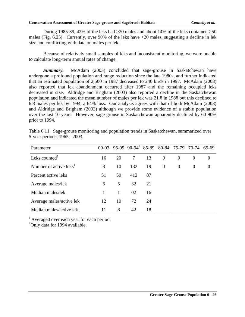
Conservation Assessment of Greater Sage-grouse and Sagebrush Habitats Connelly et al.
Greater Sage-Grouse Population 6 - 46
During 1985-89, 42% of the leks had >20 males and about 14% of the leks contained >50 males (Fig. 6.25). Currently, over 90% of the leks have <20 males, suggesting a decline in lek size and conflicting with data on males per lek.
Because of relatively small samples of leks and inconsistent monitoring, we were unable to calculate long-term annual rates of change.
Summary. McAdam (2003) concluded that sage-grouse in Saskatchewan have undergone a profound population and range reduction since the late 1980s, and further indicated that an estimated population of 2,500 in 1987 decreased to 240 birds in 1997. McAdam (2003) also reported that lek abandonment occurred after 1987 and the remaining occupied leks decreased in size. Aldridge and Brigham (2003) also reported a decline in the Saskatchewan population and indicated the mean number of males per lek was 21.8 in 1988 but this declined to 6.8 males per lek by 1994, a 64% loss. Our analysis agrees with that of both McAdam (2003) and Aldridge and Brigham (2003) although we provide some evidence of a stable population over the last 10 years. However, sage-grouse in Saskatchewan apparently declined by 60-90% prior to 1994. Table 6.11. Sage-grouse monitoring and population trends in Saskatchewan, summarized over 5-year periods, 1965 - 2003. Parameter 00-03 95-99 90-942 85-89 80-84 75-79 70-74 65-69
Leks counted1 16 20 7 13 0 0 0 0
Number of active leks1 8 10 132 19 0 0 0 0
Percent active leks 51 50 412 87
Average males/lek 6 5 32 21
Median males/lek 1 1 02 16
Average males/active lek 12 10 72 24
Median males/active lek 11 8 42 18 1 Averaged over each year for each period. 2Only data for 1994 available.

Conservation Assessment of Greater Sage-grouse and Sagebrush Habitats Connelly et al.
Greater Sage-Grouse Population 6 - 47
Fig. 6.24. Changes in lek size for sage-grouse in Saskatchewan, 1994-2003.
0
2
4
6
8
10
12
1992 1994 1996 1998 2000 2002 2004
Year
Mal
es/le
k
Fig. 6.25. Change in lek size class for Saskatchewan, summarized over 5-year periods, 1987 - 2003.
0
20
40
60
80
100
120
1985
-1989
1990
-1994
1995
-1999
2000
-2003
% in
eac
h ca
tego
ry
< 20 males 20-49 males > 49 males

Conservation Assessment of Greater Sage-grouse and Sagebrush Habitats Connelly et al.
Greater Sage-Grouse Population 6 - 48
South Dakota
Monitoring effort. South Dakota has identified 24 leks. Population monitoring efforts were sporadic and data were often collected late in the breeding season (e.g., 64% of the counts made in Butte County in 1973 [n = 11] occurred after 1 May, no lek was counted >1 time and data for 2 counts failed to differentiate between genders). Smith (2003) also cautioned against using data collected prior to 1989. Consequently, we only used lek count data obtained since 1990 to assess population trends for this state. From 1990 through 2003, the number of leks censused remained relatively stable but the number of active leks decreased by 46% (Table 6.12).
Population change. The average percent of active leks censused decreased from 87% during 1990-94 to 45% in 2000-03. The average and median males per lek also decreased by 50% and 100%, respectively (Table 6.12). The average and median males per active lek remained largely unchanged over this period. Moreover, analysis of monitoring data indicated no significant change (P = 0.40) in lek size from 1990-2003 (Fig. 6.26). This may suggest that population declines were largely due to loss of subpopulations associated with certain leks or groups of leks, likely as a result of habitat change. However, an assessment of change in proportion of lek size classes suggests a decrease of medium leks and an increase of small leks over the assessment period. In 1990-94, about 65% of the leks contained <20 males and about 35% had 20-49 males. By 200-03, about 80% of the leks contained <20 males while 20% had 20-49 males (Fig. 6.27). Because the data are somewhat ambiguous, they do not allow a meaningful assessment of population status and trends.
Summary. Connelly and Braun (1997) indicated that South Dakota breeding populations declined by 45% when they compared the long-term average of males/lek to the average for 1985-94. Although some of their analysis for South Dakota was based on questionable data, our present assessment also suggested a decline of similar magnitude. Smith (2003) reported that 12 of 25 (48%) known leks in South Dakota are currently active and that one of these leks represents a small, isolated population of sage-grouse in Fall River County. Smith (2003) also concluded that South Dakota sage-grouse populations underwent a steady decline from 1973 to 1997, with recovery from 1997 to 2002. However, he cautioned that survey efforts in South Dakota have been very inconsistent. Available data suggest that a large part of the decline was the result of loss of entire subpopulations but there is also some evidence suggesting some decline in numbers of birds associated with existing leks.
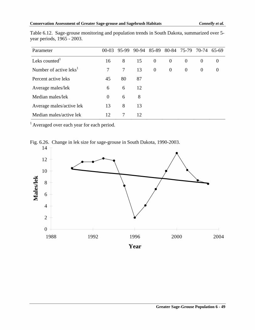
Conservation Assessment of Greater Sage-grouse and Sagebrush Habitats Connelly et al.
Greater Sage-Grouse Population 6 - 49
Table 6.12. Sage-grouse monitoring and population trends in South Dakota, summarized over 5-year periods, 1965 - 2003. Parameter 00-03 95-99 90-94 85-89 80-84 75-79 70-74 65-69
Leks counted1 16 8 15 0 0 0 0 0
Number of active leks1 7 7 13 0 0 0 0 0
Percent active leks 45 80 87
Average males/lek 6 6 12
Median males/lek 0 6 8
Average males/active lek 13 8 13
Median males/active lek 12 7 12 1 Averaged over each year for each period. Fig. 6.26. Change in lek size for sage-grouse in South Dakota, 1990-2003.
0
2
4
6
8
10
12
14
1988 1992 1996 2000 2004
Year
Mal
es/le
k

Conservation Assessment of Greater Sage-grouse and Sagebrush Habitats Connelly et al.
Greater Sage-Grouse Population 6 - 50
Fig. 6.27. Change in lek size class for South Dakota, summarized over 5-year periods, 1990 - 2003.
0
10
20
30
40
50
60
70
80
90
1990-1994 1995-1999 2000-2003
% in
eac
h ca
tego
ry
< 20 males 20-49 males 50-74 males
Utah
Monitoring effort. Utah has had a long-term extensive monitoring program for sage-grouse and has identified 254 leks in the state. Although the average number of leks monitored in the 1970-75 period increased by >160% over the average number censused in 1965-70, we were still able to use 1965-2003 as our assessment period. The average number of leks counted per 5-year period increased by 289% from 1965-70 to 2000-03 (Table 6.13). The number of active leks monitored followed the same increasing pattern as total number of leks (Table 6.13).
Population Changes. The proportion of active leks decreased somewhat over the assessment period, ranging from 89% to 72% over the 5-year periods from 1965 to 2003 (Table 6.13). Population trends indicated by average and median males per lek decreased over the assessment period by 19% and 42%, respectively (Table 6.13). However, average and median males per active lek changed little over the assessment period (Table 6.13). Monitoring data (males/lek) indicated that lek size changed significantly (r2 =0.16, P = 0.01) from 1965 to 2003 (Fig. 6.28) but these data varied greatly and should be viewed with caution.
The proportion of small leks increased somewhat over the assessment period. In general,
lek size classes fluctuated from 1965 to 2003 but there were no major changes, especially in the proportion of medium leks (Fig. 6.29). Large leks comprised <20% of the leks sampled over the 5-year periods throughout the assessment period.

Conservation Assessment of Greater Sage-grouse and Sagebrush Habitats Connelly et al.
Greater Sage-Grouse Population 6 - 51
Annual rates of change suggest a long-term decline for sage-grouse in Utah (Fig. 6.30) and support the trend information obtained from lek attendance (males/lek) and lek class size. Sage-grouse populations declined at an overall rate of 0.35% per year from 1965 to 2003. Our analysis indicated a reasonably high likelihood of density dependence for the overall assessment period (likelihood = 0.90) and for both the early (likelihood = 0.87) and late (likelihood = 0.71) periods. From 1965-85, the population declined at an average rate of 0.83% and fluctuated around a level that was approximately 1.4 times higher than the 2003 population. From 1986 to 2003, the population fluctuated around a level that was approximately 5% below the 2003 population and increased at an average rate of 0.18% per year. Populations in the early 1970s were approximately 2 times higher than current populations (Fig. 6.30). The population reached a low in the mid-1990s and has increased considerably since that time. However, previous population recoveries (late 1970s and late 1980s) did not reach levels attained in the late 1960s and early 1970s.
Summary. Connelly and Braun (1997) reported that breeding populations in Utah declined by 30% when they compared average lek size from 1985-94 to long-term averages. However, production increased by 1% when 1985-94 data were compared to long-term averages (Connelly and Braun 1997). Beck et al. (2003) reported that males per lek declined for all populations in Utah from 1971 to 2000 but they also provided some evidence indicating populations in 3 counties may be stable or increasing. Our results suggested that population declines may have been greater than those reported by Connelly and Braun (1997) and Beck et al. (2003) but supported their overall conclusion of a long-term population decline. Table 6.13. Sage-grouse monitoring and population trends in Utah, summarized over 5-year periods, 1965 - 2003. Parameter 00-03 95-99 90-94 85-89 80-84 75-79 70-74 65-69
Leks counted1 144 118 99 109 94 108 97 37
Number of active leks1 111 85 82 84 74 92 83 33
Percent active leks 77 72 83 77 79 86 85 89
Average males/lek 21 15 19 19 19 24 23 26
Median males/lek 11 8 10 11 12 13 16 19
Average males/active lek 28 21 22 24 24 28 27 30
Median males/active lek 19 14 15 16 17 17 20 21 1 Averaged over each year for each period.

Conservation Assessment of Greater Sage-grouse and Sagebrush Habitats Connelly et al.
Greater Sage-Grouse Population 6 - 52
Fig. 6.28. Changes in lek size for sage-grouse in Utah, 1965 - 2003.
0
5
10
15
20
25
30
35
40
1964 1969 1974 1979 1984 1989 1994 1999 2004
Year
Mal
es/le
k
Fig. 6.29. Change in lek size class for Utah, summarized over 5-year periods, 1965 - 2003.
0
10
20
30
40
50
60
70
1965
-1969
1970
-1974
1975
-1979
1980
-1984
1985
-1989
1990
-1994
1995
-1999
2000
-2003
% in
eac
h ca
tego
ry
< 20 males 20-49 males > 49 males

Conservation Assessment of Greater Sage-grouse and Sagebrush Habitats Connelly et al.
Greater Sage-Grouse Population 6 - 53
Fig. 6.30. Change in the population index for greater sage-grouse in Utah, 1965 - 2003.
0
5 0
1 0 0
1 5 0
2 0 0
2 5 0
1 9 6 4 1 9 6 9 1 9 7 4 1 9 7 9 1 9 8 4 1 9 8 9 1 9 9 4 1 9 9 9 2 0 0 4
Y ear
Perc
ent o
f 200
3 po
pula
tion
Popu la tion indexT rendE arly density dependentL ate density dependent
Washington
Monitoring effort. Washington has identified 62 leks and has had a long-term monitoring program in place. Thus, we used 1965-2003 as the assessment period. The average number of leks counted per 5-year period increased substantially over the assessment period (Table 6.14). In 1965-69, an average of 3 leks per year were censused but by 2000-03, an average of 47 leks per year were counted, an increase of >1400%. The average number of active leks counted per 5-year period also increased by >500%. Observers in Washington generally followed established procedures for lek census and attempted to count leks >3 times over an approximately 5-week period from mid-March to early May.
Population Change. The proportion of active leks decreased over the assessment period, averaging between 92% and 100% from 1965 to 1984 but decreased to 41% by 2000-2003 (Table 6.14). Population trends indicated by average and median males per lek also decreased over the assessment period by >75% (Table 6.14). Average and median males per active lek also indicated a decline over the assessment period, and both decreased by about 45% (Table 6.14). Monitoring data indicated that lek size decreased significantly (r2 =0.69, P = 0.00) from 1965 to 2003 (Fig. 6.31). Although some subpopulations have disappeared (Schroeder et al. 2000), it also appears that the number of breeding birds associated with some leks has declined substantially.
Relatively few leks were censused from 1965 to 1984 (Table 6.14) so information on changes in lek size classes during these years should be viewed with caution. From 1985 to

Conservation Assessment of Greater Sage-grouse and Sagebrush Habitats Connelly et al.
Greater Sage-Grouse Population 6 - 54
2003, the proportion of small leks remained relatively steady while the proportion of medium leks increased. Over the same period, large leks decreased from about 18% to 3% (Fig. 6.32).
Annual rates of change suggest a long-term decline for sage-grouse in Washington (Fig.
6.33) and support the trend information obtained from lek attendance (males/lek) and lek class size. Sage-grouse populations declined at an overall rate of 4.79% per year from 1965 to 2003. Our analysis indicated a high likelihood of density dependence for the overall assessment period (likelihood = 0.96) and for both the early (likelihood = 0.83) and late (likelihood = 0.84) periods. From 1965-85, the population declined at an average rate of 8.73% and fluctuated around a level that was approximately 1.4 times higher than the 2003 population. From 1986 to 2003, the population fluctuated around a level that was approximately 1.2% above the 2003 population and had an average change of –0.20% per year. Populations in the late 1960s and early 1970s were approximately 4-6 times higher than 2003 populations (Fig. 6.33).
Summary. The relatively large decrease in active leks over the assessment period may be due to inconsistent data collection (Schroeder et al. 2000), a tendency of early biologists to only census active leks or an actual decrease in the number of active leks. Most likely it was a combination of these factors. Connelly and Braun (1997) reported that sage-grouse populations had declined by 47% in Washington. Schroeder et al. (2000) reported that sage-grouse in Washington declined by at least 77% from 1960 to 1999 and that the current populations only occupy about 8% of historic range. Our current analysis suggests that Connelly and Braun’s (1997) estimate was likely too conservative and generally supported Schroeder et al.’s (2000) estimate. Table 6.14. Sage-grouse monitoring and population trends in Washington, summarized over 5-year periods, 1965 - 2003. Parameter 00-03 95-99 90-94 85-89 80-84 75-79 70-74 65-69
Leks counted1 47 31 25 20 18 15 14 3
Number of active leks1 20 18 16 14 16 14 13 3
Percent active leks 41 56 62 71 91 92 99 100
Average males/lek 8 11 13 17 26 15 24 33
Median males/lek 0 5 4 6 23 13 20 31
Average males/active lek 18 20 20 23 28 16 25 33
Median males/active lek 17 18 14 14 24 14 20 31 1 Averaged over each year for each period.

Conservation Assessment of Greater Sage-grouse and Sagebrush Habitats Connelly et al.
Greater Sage-Grouse Population 6 - 55
Fig. 6.31. Change in lek size for sage-grouse in Washington, 1965 - 2003.
0
5
10
15
20
25
30
35
40
1964 1969 1974 1979 1984 1989 1994 1999 2004
Year
Mal
es/le
k
Fig. 6.32. Change in lek size class for Washington, summarized over 5-year periods, 1965 - 2003.
0
10
20
30
40
50
60
70
80
1965
-1969
1970
-1974
1975
-1979
1980
-1984
1985
-1989
1990
-1994
1995
-1999
2000
-2003
% in
eac
h ca
tego
ry
< 20 males 20-49 males > 49 males

Conservation Assessment of Greater Sage-grouse and Sagebrush Habitats Connelly et al.
Greater Sage-Grouse Population 6 - 56
Fig. 6.33. Change in the population index for greater sage-grouse in Washington, 1965 -2003.
0
100
200
300
400
500
600
700
1964 1969 1974 1979 1984 1989 1994 1999 2004
Year
Perc
ent o
f 200
3 po
pula
tion
Population indexTrendEarly density dependentLate density dependent
Wyoming
Monitoring effort. Wyoming has had a long-term extensive monitoring program for sage-grouse and has identified 1,454 leks in the state. We used 1965-2003 as our assessment period. The average number of leks censused per 5-year period increased by > 1000% from 1965 to 2003 and ranged from 80 to 945 over the assessment period (Table 6.15). The average number of active leks censused per 5-year period was similarly high, ranging from 58 to 672. Observers in Wyoming generally followed established procedures for lek census and attempted to count leks >3 times over an approximately 5-week period from late March to early May.
Population Changes. The proportion of active leks remained relatively stable over the
assessment period, ranging from 63% to 78% from 1965 to 2003 (Table 6.15). Population trends indicated by average and median males per lek decreased over the assessment period by 49% and 48%, respectively (Table 6.15). Average and median males per active lek also declined by 48% and 43%, respectively, over the assessment period (Table 6.15). Monitoring data (males/lek) indicated that lek size significantly decreased (r2 =0.49, P = 0.00) from 1965 to 2003 (Fig. 6.34).
There appeared to be an overall decline in lek size. Beginning in the early 1980s, the
proportion of small leks increased. There also appeared to be an decrease in large leks from the late 1960s to the late 1990s (Fig. 6.35). However, the proportion of medium leks remained relatively stable, varying between about 30% and 40% over the assessment period (Fig. 6.35).

Conservation Assessment of Greater Sage-grouse and Sagebrush Habitats Connelly et al.
Greater Sage-Grouse Population 6 - 57
Annual rates of change suggest a long-term decline for sage-grouse in Wyoming (Fig. 6.36) and support the trend information obtained from lek attendance (males/lek) and lek class size. Sage-grouse populations declined at an overall rate of 5.22% per year from 1968 to 2003. Our analysis indicated a high likelihood of density dependence for the overall assessment period (likelihood = 0.99) and for both the early (likelihood = 0.93) and late (likelihood = 0.84) periods. From 1968-86, the population declined at an average rate of 9.66% and fluctuated around a level that was approximately 19% below the 2003 population. From 1987 to 2003, the population fluctuated around a level that was approximately 2% below the 2003 population and had an average change of 0.33% per year. Lows were reached in the mid-1990s and there has been some gradual increase in numbers since that time.
Summary. Connelly and Braun (1997) indicated that sage-grouse breeding populations had declined by 17% when they compared the long-term average of males/lek to the average obtained from 1985-94 data. A similar analysis suggested that production declined by 33% (Connelly and Braun 1997). Our analysis suggests that the decline was considerably greater than that reported by Connelly and Braun (1997). However, this may be due to our use of a larger and more complete data set as well as the addition of 9 more years of data. Our analysis generally supports the previous finding of a declining sage-grouse population. Additionally, lek surveys and counts were recently completed in an area that was intensively studied in the late 1940s and early 1950s (Patterson 1952). In 1949, 3,118 males were counted on 42 leks (74 males/lek). In 2003, 40 of the 42 leks were unoccupied but seven other leks were documented that were either not present in 1949 or not known to Patterson (1952). Thus, there were 9 active leks in this area in 2003 (a 79% decline) and 318 males (35 males/lek) were counted on these leks, indicating a 90% decline in the population (Wyoming Department of Game and Fish, personal correspondence, 2004). Table 6.15. Sage-grouse monitoring and population trends in Wyoming, summarized over 5-year periods, 1965 - 2003. Parameter 00-03 95-99 90-94 85-89 80-84 75-79 70-74 65-69
Leks counted1 945 674 568 482 355 144 89 80
Number of active leks1 672 428 384 360 264 96 69 58
Percent active leks 71 63 68 75 75 66 78 73
Average males/lek 19 13 15 17 21 23 24 37
Median males/lek 11 6 8 12 14 12 16 21
Average males/active lek 26 20 22 23 29 35 31 50
Median males/active lek 20 14 16 18 21 25 23 35 1 Averaged over each year for each period.
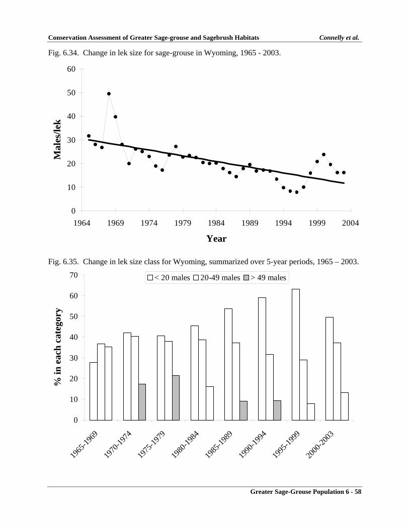
Conservation Assessment of Greater Sage-grouse and Sagebrush Habitats Connelly et al.
Greater Sage-Grouse Population 6 - 58
Fig. 6.34. Change in lek size for sage-grouse in Wyoming, 1965 - 2003.
0
10
20
30
40
50
60
1964 1969 1974 1979 1984 1989 1994 1999 2004
Year
Mal
es/le
k
Fig. 6.35. Change in lek size class for Wyoming, summarized over 5-year periods, 1965 – 2003.
0
10
20
30
40
50
60
70
1965
-1969
1970
-1974
1975
-1979
1980
-1984
1985
-1989
1990
-1994
1995
-1999
2000
-2003
% in
eac
h ca
tego
ry
< 20 males 20-49 males > 49 males

Conservation Assessment of Greater Sage-grouse and Sagebrush Habitats Connelly et al.
Greater Sage-Grouse Population 6 - 59
Fig. 6.36. Change in the population index for greater sage-grouse in Wyoming, 1968-2003.
0
100
200
300
400
500
600
700
1964 1969 1974 1979 1984 1989 1994 1999 2004
Year
Perc
ent o
f 200
3 po
pula
tion
Population indexTrendEarly density dependentLate density dependent
Range-Wide
Populations. Previous sections described sage-grouse populations within each state and province supporting this species. However, many populations overlap state boundaries (Schroeder et al. 2004) and may be subject to different environmental and management variables. Thus, we also provide an overall review of sage-grouse population data and, where possible, examine population changes without regard to political boundaries.
We based our analysis on 41 relatively discrete populations and 24 subpopulations of greater sage-grouse in western North America (Table 6.16). Many of these appear to be spatially isolated while narrow corridors connect other populations (Fig. 6.37). The most isolated populations occur in parts of Colorado, Utah, Nevada, California, and Washington.

Conservation Assessment of Greater Sage-grouse and Sagebrush Habitats Connelly et al.
Greater Sage-Grouse Population 6 - 60
Table 6.16. General description and justification for delineation of greater sage-grouse breeding populations and subpopulations in North America (also see Figure 6.37). Population
Subpopulation Separation from adjacent populationsa
Fragmentation within populationb Brief description of population and justification for its delineation
Baker OR ~30 km N.A. Small population in Baker County OR. It appears separated by cropland from the nearest population, E-Central OR.
Bannack MT ~30–50 km and Continental Divide
N.A. Small population E of Lemhi Pass near Bannack MT. It appears separated from 4 adjacent populations by distance, narrow corridors, and the continental divide.
Belt Mountains MT ~70 km along narrow corridor
~20-30 km Small population or populations near Belt Mountains MT. In addition to being separated from the adjacent Central MT population, it also appears characterized by internal fragmentation.
Central OR ~30 km ~20-30 km Population in central OR is separated by distance and topography from Lake Area OR/NE CA/NW NV and E-Central OR populations. Fragmentation within population is substantial.
Eagle/S Routt CO ~20-30 km and mountains
Population linear Small population along Colorado River in Eagle and S Routt counties CO. It appears isolated from 3 adjacent populations by both distance and topography.
E Tavaputs Plateau UT
~50 km N.A. Small population on E Tavaputs Plateau UT. It appears separated from adjacent populations by > 50 km.
E-Central ID ~30-50 km ~10-20 km on periphery
Population E of Snake River in E-central ID. Population appears isolated by distance, topography, and habitat.
Garfield CO ~40 km N.A. Small population in Garfield County CO appears isolated from both Eagle/S Routt CO and Piceance CO populations.
Great Basin Core ~20-60 km and topography
~10-30 km Large population in NV, SE OR, NE CA, SW ID, and NW UT. Natural fragmentation within population is common. Seven subpopulations have been delineated.
Central NV N.A. ~20-30 km throughout
Large population in central NV is loosely connected with SE NV/SW UT and NE NV/S-Central ID/NW UT. Fragmentation within population and among adjacent populations is substantial.
E-Central OR ~10-30 km ~10-20 km Population in E-central OR is loosely connected with Lake Area OR/NE CA/NW NV and N-Central NV/SE OR/SW ID populations. Some internal fragmentation is also apparent.
Lake Area OR/NE CA/NW NV
~20-50 km ~20-30 km Large population in NE CA, NW NV, and S-central OR. Population appears loosely connected with S-Central OR/N-Central NV and E-Central OR. Some peripheral areas in NE CA may be partially fragmented.
N-Central NV/SE OR/SW ID
~10-20 km N.A. Loosely connected with NE NV/S-Central ID/NW UT, E-Central OR, and S-Central OR/N-Central NV populations.
NE NV/S-Central ID/NW UT
~10-20 km ~10-20 Large population in NE NV, S-central ID, and NW UT. Population appears loosely connected with N-Central NV/SE OR/SW ID and Central NV populations.
S-Central OR/N-Central NV
~20-30 km ~10-20 km Population straddling the border of NV and OR. Appears loosely connected with 4 adjacent populations.
SE NV/SW UT N.A. ~10-20 km Large naturally fragmented population in SE NV that appears loosely interconnected with Central NV population.
Gunnison Range UT ~200 km N.A. Small translocated population of greater sage-grouse in SE UT within population of Gunnison sage-grouse. It is also isolated from nearest Gunnison sage-grouse populations by > 70 km.
Jackson Hole WY ~50 km ~20-30 km Small isolated population in Jackson Hole WY area. Population also appears internally fragmented.
Klamath OR/CA ~50 km ~20-30 km Small population on E side of Klamath Basin OR and CA. Population also appears internally fragmented.
Laramie WY ~30 km and mountains N.A. Small population SW of Laramie WY. Appears isolated by both distance and topography from adjacent populations.

Conservation Assessment of Greater Sage-grouse and Sagebrush Habitats Connelly et al.
Greater Sage-Grouse Population 6 - 61
Middle Park CO ~20-30 km and mountains
~20 km Population in Middle Park CO appears isolated from North Park CO and Garfield CO populations.
Moses Coulee WA ~50 km and Columbia River
~10-20 km Population along Moses Coulee in N-central WA is isolated by distance and topography from Yakima WA population. Peripheral parts of population are extirpated.
MT/ND/NW SD ~30-40 km ~10-20 km Population centered in SW ND and NW SD is largely isolated by distance and habitat from E-Interior MT/NE Tip WY population. Internal fragmentation is also apparent.
N Mono Lake CA/NV
~20-40 km and mountains
~10-20 km Population on N side of Mono Lake area in CA and NV is relatively isolated from adjacent populations by both distance and topography. There is some natural internal fragmentation also.
NE-Interior UT ~30-50 km ~10-30 Population in NW-interior portion of Utah appears isolated by both distance and topography from adjacent populations. Natural fragmentation within population is also a factor.
Northern Montana ~20 km and Missouri River
~20-40 km Large population N of Missouri River in N-central MT, SE AB, and SW SK. Divided into 3 subpopulations.
AB/SW SK/MT
~20 km along a narrow corridor
N.A. Population in SE AB, SW SK and N edge of MT. It is separated from other birds in Saskatchewan by ~50 km
N-Central MT ~20 km ~20-30 km Large population N of Missouri River in N-central MT. Loosely connected with populations to N, but separated from populations to S by Missouri River.
S-Central SK/MT
~20-40 km ~20-30 km Population straddling the border of SK and MT. Population appears to be fragmented within by distance and habitat.
NW-Interior NV ~20-30 km ~20-30 km Topographically dispersed population in interior NV. It appears largely isolated from 5 adjacent populations.
Piceance CO ~30-40 km N.A. Small population in the Piceance Basin CO. Adjacent populations appear isolated by both distance and topography.
Pine Nut NV ~50-60 km and valleys N.A. Small population in Pine Nut Mountains NV. Appears relatively isolated from adjacent populations by both distance and topography.
Quinn Canyon Range NV
~50-80 km and valleys N.A. Small population in the Quinn Canyon Range NV. Appears isolated from adjacent populations by both distance and topography.
Red Rock MT ~20-40 km and mountains
~10-20 km Small, naturally fragmented population in SW Montana on N side of Monida Pass. Population appears isolated by distance and topography from adjacent populations.
S Mono Lake CA ~20-50 km and mountains
~10-20 km Small population on S side of Mono Lake area in CA appears relatively isolated from adjacent populations by both distance and topography. There is some natural internal fragmentation also.
S White River UT ~40-50 km N.A. Small population S of White River UT. It is separated from adjacent populations by > 40 km.
Sanpete/Emery UT ~50-60 km ~20 km Small population in central UT that is isolated by both distance and topography.
Sawtooth ID ~70-80 km ~10-20 km Small isolated population near Stanley, ID in Sawtooth Mountains.
S-Central UT ~50-70 km and mountains
~20-40 km Clearly isolated population in S-central UT. Population appears to have a high degree of natural fragmentation within it.
Snake, Salmon, and Beaverhead
~20-40 km ~10-30 km Large population along upper Snake, Salmon, and Beaverhead watersheds. Six subpopulations appear loosely connected through mountain valleys and passes.
Big Lost ID ~10 km along narrow corridors
Population linear Population follows Big Lost and Willow Creek Valleys in ID. Connected with Little Lost ID and N-Side Snake ID populations along narrow corridors.
Lemhi-Birch ID
~20 km and topography Population linear Population along Lemhi and Birch Creek Valleys ID. Appears largely isolated by both distance and topography.
Little Lost ID ~20 km and narrow corridors
Population linear Population along Little Lost and Pahsimeroi valleys ID. Population may be loosely connected with Big Lost ID and Lemhi-Birch ID populations along narrow corridors.
N Side Snake ID
~10-30 km ~10 km Large population on N side of Snake River ID. Loosely connect along narrow corridor with Big Lost ID population.

Conservation Assessment of Greater Sage-grouse and Sagebrush Habitats Connelly et al.
Greater Sage-Grouse Population 6 - 62
Upper Snake ID
~20-40 km and mountains
N.A. Population along upper Snake River ID. Population appears mostly isolated from adjacent populations.
Summit/Morgan UT ~20-40 km and mountains
N.A. Small population in NE UT appears separated from SW WY/NW CO/NE UT/SE ID by both distance and topography.
Tooele/Juab UT ~40 km ~10-20 km Small isolated population in central UT. Population also appears naturally fragmented.
Twin Bridges MT ~60 km N.A. Small isolated population in SW MT.
Warm Springs Valley NV
~30-60 km and valleys ~10-20 km Small, fragmented, and isolated population along the W edge of NV.
Weiser ID ~20 km N.A. Small and mostly isolated population in Weiser area ID.
White Mountains NV/CA
~50 km and topography N.A. Small and isolated population in White Mountains straddling border of CA and NV.
White River CO ~30-40 km and mountains
N.A. Small isolated population along White River CO.
Wisdom MT ~4-60 km N.A. Small isolated population in SW MT.
Wyoming Basin ~20-30 km and topography
~10-20 km Massive population centered in WY. Seven subpopulations have been delineated.
Dinosaur UT/CO
~10-20 km along narrow corridors
~10-20 km Population largely between Yampa and White rivers along UT-CO border. Appears mostly separated from 6 adjacent populations by both distance and topography.
Fall River SD/E-Edge WY
~10-20 km 10-20 km Small population in SW SD and E-edge WY may be loosely connected along narrow corridor to E-Interior MT/NE Tip WY population. Fragmentation within population is apparent.
NE WY/SE MT
~10-20 km ~10-20 Large population primarily in NE WY. Population appears continuous within and loosely connected with adjacent populations.
North Park CO/WY
~10 km along narrow corridor
N.A. Population in North Park CO appears connected with S-Central WY/N-Central CO population along narrow North Platte River corridor. Other adjacent populations separated by topography.
S-Central MT/N-Central WY
~10-40 km ~20-30 km Large population primarily in N-central WY. Appears isolated from Central MT population, but loosely interconnected with NE WY/SE MT and S-Central WY/N-Central CO populations. There may be isolated pockets within the overall population.
S-Central WY/N-Central CO
N.A. ~10-20 km Large population primarily in S-central WY. It appears loosely connected with all adjacent populations.
SW WY/NW CO/NE UT/SE ID
N.A. N.A. Large population primarily in SW WY. Population appears loosely connected with S-Central WY/N-Central CO and Dinosaur UT/CO.
Yakima WA ~50 km and Columbia River
N.A. Population near Yakima in S-central WA is isolated by distance and topography from Moses Coulee WA population. Peripheral parts of population are extirpated.
Yellowstone watershed
~20-30 km ~20-30 km Large population in central and SE MT. Mostly separated from adjacent populations by distance and topography.
Central MT N.A. ~20-30 km on periphery
Large population in central MT is loosely connected with E-Interior MT/NE Tip WY population. Population is separated from N-Central MT population by ~20-30 km and Missouri River.
E-Interior MT/NE Tip WY
N.A. ~20-30 km on periphery
Large population primarily in SE Montana. It appears loosely connected with Central MT population, but separated from N-Central MT, MT/ND/NW SD, and NE WY/SE MT populations by distances of 20-30 km.
aN.A. (not apparent) was used to describe several populations where separation and/or isolation from adjacent populations was not apparent. These populations were delineated on the basis of their large size and broader differences associated with region. bN.A. (not apparent) was used to describe populations where fragmentation within the population was not apparent.

Conservation Assessment of Greater Sage-grouse and Sagebrush Habitats Connelly et al.
Greater Sage-Grouse Population 6 - 63
Fig. 6.37. Discrete populations and subpopulations of sage-grouse in western North America.
Of the 7 floristic regions that support sage-grouse, the Snake River Plain and southern
Great Basin regions contain the greatest number of populations, 16 and 13, respectively (Table 6.17). The Columbia Basin only has 2 populations.

Conservation Assessment of Greater Sage-grouse and Sagebrush Habitats Connelly et al.
Greater Sage-Grouse Population 6 - 64
Table 6.17. Categorization of greater sage-grouse populations and subpopulations by floristic regions in North America (partly following Miller and Eddleman 2001). Great Plains Wyoming Basin Snake River Plain Columbia
Basin Northern Great Basin
Southern Great Basin
Colorado Plateau
MT/ND/NW SD
Belt Mountains MT Baker OR Moses Coulee WA
Central OR Summit/Morgan UT
E Tavaputs Plateau UT
AB/SW SK/MT Eagle/S Routt CO Bannack MT Yakima WA Lake Area OR/NE CA/NW NV
Quinn Canyon Range NV
Garfield CO
Fall River SD/E-Edge WY
SW WY/NW CO/NE UT/SE ID
E-Central ID S-Central OR/N-Central NV
N Mono Lake CA/NV
Gunnison Range UT
S-Central SK/MT
S-Central MT/N-Central WY
NE NV/S-Central ID/NW UT
Klamath OR/CA Sanpete/Emery UT
White River CO
E-Interior MT/NE Tip WY
S-Central WY/N-Central CO
N-Central NV/SE OR/SW ID
Warm Springs Valley NV
White Mountains NV/CA
S White River UT
NE WY/SE MT Jackson Hole WY E-Central OR Central NV Piceance CO
N-Central MT North Park CO/WY Red Rock MT SE NV/SW UT
Central MT Laramie WY Sawtooth ID S Mono Lake CA
Middle Park CO Big Lost ID NE-Interior UT
Dinosaur UT/CO Lemhi-Birch ID S-Central UT
Little Lost ID Pine Nut NV
N-Side Snake ID Tooele/Juab UT
Twin Bridges MT NW-Interior NV
Upper Snake ID
Weiser ID
Wisdom MT
Monitoring. Virtually all states and provinces have increased monitoring efforts, especially over the last 10 years (Table 6.18; also Appendix 3, Fig. A3.2). Our analysis indicated that a total of 2,637 leks are now censused annually. This is about 30% more than the number reported by the agencies in their response to the questionnaire (see previous section on Population Databases in this chapter). Range-wide, population monitoring efforts increased by 729% over the long-term. The largest increases in effort have occurred Montana and Wyoming, 2 of the key sage-grouse states. Montana had 2 periods when efforts increased substantially; 1965-69 to 1975-79 when the average number of leks monitored increased by >700% and 2000-03 when the average number of leks censused tripled over the number censused in 1995-99. Increasing census efforts may be related to concerns over sage-grouse numbers during the late 1960s and early to mid 1970s. During this period, data from most states indicated declining sage-grouse populations (see state accounts in this Chapter). However, this seems an unlikely explanation for increased censusing because these declines did not appear to be widely recognized at that time. From the 1950s through the 1980s, the Western States Sage and Columbian Sharp-tailed Grouse Technical Committee compiled unpublished qualitative reports from western states and provinces on the status of sage-grouse populations (Sage Grouse Questionnaire, Numbers I-XXIII, Western States Sage and Columbian Sharp-tailed Grouse Technical Committee, unpublished reports). Qualitative information obtained from these

Conservation Assessment of Greater Sage-grouse and Sagebrush Habitats Connelly et al.
Greater Sage-Grouse Population 6 - 65
questionnaires for 1965 to 1979 does not show a clear recognition of population trends throughout western North America (Table 6.19). From 1965 through 1979, most states and provinces indicated populations were stable to increasing, in general disagreement with population data we obtained from these states and provinces. Moreover, New Mexico reported that sage-grouse populations in that state were stable or increasing from 1956 through 1975 even though Aldrich (1963) indicated the species had been extirpated from that state. Additionally, Reese and Connelly (1997) reported introductions of greater sage-grouse into the former range of Gunnison sage-grouse in New Mexico in the 1930s, 1940s, and 1960s, further suggesting that sage-grouse populations in New Mexico were likely declining for a relatively long period of time. Currently, neither species of sage-grouse occurs in New Mexico (Schroeder et al. 2004). Similarly, Montana reported stable sage-grouse populations for each year from 1968 through 1975, but lek size and population trend data indicated increasing and decreasing populations over this period (see Figures 6.12 and 6.14). Thus, it is more likely that increases in monitoring effort were the result of changes in program priorities or interests of individual agency biologists.
Although monitoring efforts have increased, there still appears to be a reluctance by some states/provinces to use established and accepted monitoring techniques (Jenni and Hartzler 1978, Emmons and Braun 1984, Connelly et al. 2003). Although data collected within these states or provinces may indicate population trends over time, these different methods confound attempts to make comparisons with other states. Table 6.18. Changes in long-term monitoring efforts for states and provinces supporting sage-grouse populations. State/Province Leks Censused 1965-69 Leks Censused 2000-2003 % Change Alberta 14 (starting 1975-1979) 29 107 California 9 45 400 Colorado 66 171 159 Idaho 74 319 331 Montana 13 546 4,100 Nevada 22 182 727 North Dakota 19 27 42 Oregon 18 153 750 Saskatchewan 13 (starting 1985-1989) 16 23 South Dakota 15 (starting 1990-1994) 16 7 Utah 37 144 289 Washington 3 47 1,467 Wyoming 80 945 1,081 Average 729

Conservation Assessment of Greater Sage-grouse and Sagebrush Habitats Connelly et al.
Greater Sage-Grouse Population 6 - 66
Table 6.19. Qualitative assessment of population trends by states and provinces for 5-year periods, 1965-69 to 1975-79.1
State/Province 1965-69 1970-74 1975-79 Overall Alberta I/S2 S/D D D California S S S S Colorado S S/D I S/I Idaho S/I D I D Montana S S S S Nevada I S/D S/I S/I North Dakota S S D S Oregon D D S D Saskatchewan S/I S S S South Dakota S S D D Utah I S I I Washington S S/D D S Wyoming S/I S/D S S % Decreasing 8 15 31 31
1 Information obtained from Western States Sage and Columbian Sharp-tailed Grouse Technical Committee Sage Grouse Questionnaire, Numbers I-XXIII. 2 D = decreasing; I = increasing; S = stable.
Lek Distribution and Numbers. Throughout western North America 5,585 sage-grouse leks have been identified since agencies first began routine monitoring of this species. The number of leks counted has increased dramatically from 1965 to 2003 and an average of 2,637 leks/year and 48,378 males were counted from 2000 to 2003 (Table 6.20). In 2003, a total of 50,566 male sage-grouse were counted on leks throughout western North America. Not all leks are currently active and many have been inactive for years. The total number of leks that has been extirpated is unknown and hinders our attempts to fully understand the magnitude of change in sage-grouse populations. Although leks have become inactive throughout the species’ range, the distribution of inactive leks appears clustered rather than widespread (Fig. 6.40). Proportionally, the largest number of inactive leks appears to occur in Colorado, Utah and Washington. Table 6.20. Average number of leks and male sage-grouse counted by 5-year period, 1965-2003. Parameter 1965-69 1970-74 1975-79 1980-84 1985-89 1990-94 1995-99 2000-03 Leks 351 510 676 1,016 1,162 1,318 1,689 2,637 Active leks 299 434 565 828 828 961 1,182 1,925 Males counted 11,402 13,573 17,239 21,985 22,278 21,783 23,687 48,378

Conservation Assessment of Greater Sage-grouse and Sagebrush Habitats Connelly et al.
Greater Sage-Grouse Population 6 - 67
Fig. 6.40. Distribution of active and inactive sage-grouse leks in western North America, spring 2000. The range of the Gunnison sage-grouse in SW Colorado and SE Utah was not included in this analysis although the distribution is shown.
Population Status and Change. Generally, the proportion of small leks has increased
over the assessment periods for most states and provinces while the proportion of large leks has decreased. Although some states have monitored sage-grouse populations since the 1940s, little is known about the protocols used or consistency of monitoring efforts during those early years. There was much more variation associated with estimates of lek size in the 1940s and 1950s and variation was noticeably reduced by the mid-1960s (Fig. 6.41). An examination of all trend data from the mid 1940s to 2003 suggests a substantial decline in the overall sage-grouse population in North America. However, because data collected in the 1940s and 1950s is highly variable (Fig. 6.41) and may have been collected in a somewhat haphazard fashion, there is no means of assessing the true magnitude of the population change.
Eleven of 13 (85%) states and provinces showed significant long-term declines in size of
active leks (Table 6.21). Similarly, eight of 10 states (80%) showed population declines over that time frame (Table 6.21). Two of 10 (20%) appeared to be stable or slightly increasing. Only California had an increase in both the population index and lek size.

Conservation Assessment of Greater Sage-grouse and Sagebrush Habitats Connelly et al.
Greater Sage-Grouse Population 6 - 68
Fig. 6.41. Average active lek size (with 95% C.I.) for greater sage-grouse in North America by 5-year intervals, 1945-2003.
0
20
40
60
80
100
120
1945
-1949
1950
-1954
1955
-1959
1960
-1964
1965
-1969
1970
-1974
1975
-1979
1980
-1984
1985
-1989
1990
-1994
1995
-1999
2000
-2003
Ave
rage
mal
es/le
k
Table 6.21. Summary table for regression analysis of maximum counts on active leks and average instantaneous rates of population change by state or province. Data for states and provinces other than Alberta, Saskatchewan, and South Dakota are for 1965-2003.
Average lek size in relation to year State/province Intercept Slope r2 F P
Average instantaneous rate of population change
Alberta 923.21 -0.455 0.083 26.648 < 0.001 ID1 California -183.29 0.108 0.001 0.885 0.347 +0.7 Colorado 841.69 -0.407 0.025 57.342 < 0.001 +1.0 Idaho 1037.07 -0.507 0.035 186.369 < 0.001 -1.5 Montana 330.51 -0.155 0.006 33.090 < 0.001 -1.6 Nevada 920.43 -0.451 0.039 86.553 < 0.001 -2.1 North Dakota 243.50 -0.116 0.013 8.596 0.004 -2.8 Oregon 223.61 -0.101 0.002 3.025 0.082 -3.5 Saskatchewan 2513.14 -1.252 0.135 24.406 < 0.001 ID1 South Dakota 558.68 -0.274 0.069 18.817 < 0.001 ID1 Utah 245.11 -0.111 0.002 6.396 0.012 -0.35 Washington 421.31 -0.201 0.012 6.404 0.012 -4.79 Wyoming 755.92 -0.367 0.017 194.033 < 0.001 -5.2 1 Insufficient data to calculate population index.

Conservation Assessment of Greater Sage-grouse and Sagebrush Habitats Connelly et al.
Greater Sage-Grouse Population 6 - 69
Trends for distinct populations were similar to those of states. We had sufficient data to assess trends in maximum lek counts for 34 of the 41 (83%) identified populations (Table 6.22). Twenty-one of 22 significant correlations were negative (Table 6.22). Within the five largest populations, 16 of 17 subpopulations with significant correlations were also negative. We also examined the trend in maximum lek counts by region (Table 6.23). Lek counts in 5 of 7 (71%) floristic regions declined significantly over the long-term and two remained unchanged (also see appendix 6). Characteristics of sage-grouse populations and subpopulations are summarized in appendices 4 and 5. Table 6.22. Summary table for regression analysis of maximum counts on active leks by populations and subpopulations between 1965-2003 (not all years available for each population or subpopulation). Significant slopes are in bold. Population/subpopulation Intercept Slope r2 F P Baker OR 624.71 -0.300 0.008 0.520 0.473 Bannack MT 1019.95 -0.502 0.134 21.879 < 0.001 Belt Mountains MT 2087.17 -1.036 0.328 36.173 < 0.001 Central OR 415.01 -0.200 0.027 23.811 < 0.001 E Garfield CO 427.43 -0.214 0.107 0.120 0.788 Eagle/S Routt CO 908.65 -0.449 0.149 17.353 < 0.001 East Tavaputs Plateau UT 577.54 -0.288 0.145 4.250 0.050 E-Central ID 654.92 -0.322 0.103 14.365 < 0.001 Great Basin Core 627.10 -0.303 0.014 80.572 < 0.001 Central NV 536.42 -0.257 0.017 11.885 < 0.001 E-Central OR 677.28 -0.329 0.020 5.144 0.024 Lake Area OR/NE CA/NW NV 13.99 0.011 0.000 0.008 0.928 N-Central NV/SE OR/SW ID 1154.59 -0.568 0.057 32.042 < 0.001 NE NV/S-Central ID/NW UT 960.11 -0.471 0.041 99.280 < 0.001 S-Central OR/N-Central NV 3706.12 -1.852 0.264 7.877 0.010 SE NV/SW UT 553.73 -0.270 0.021 21.453 < 0.001 Gunnison Range UT 1199.43 -0.599 0.361 6.201 0.030 Jackson Hole WY 2119.60 -1.052 0.061 5.845 0.018 Klamath OR/CA -609.59 0.310 0.303 6.963 0.018 Laramie WY 3270.96 -1.643 0.375 16.782 < 0.001 Middle Park CO 443.86 -0.214 0.024 6.183 0.014 Moses Coulee WA 414.93 -0.198 0.013 5.384 0.021 MT/ND/NW SD 170.86 -0.079 0.006 5.469 0.020 N Mono Lake CA/NV 1083.41 -0.531 0.053 15.571 < 0.001 NE Interior UT 670.867 -0.328 0.023 8.328 0.004 Northern Montana -4.98 0.014 0.000 0.064 0.800 AB/SK/MT 1041.34 -0.515 0.108 43.980 < 0.001 N-Central MT -652.42 0.340 0.024 14.342 < 0.001

Conservation Assessment of Greater Sage-grouse and Sagebrush Habitats Connelly et al.
Greater Sage-Grouse Population 6 - 70
S-Central SK/MT 2631.30 -1.310 0.171 26.616 < 0.001 NW-Interior NV -677.96 0.346 0.012 0.684 0.411 Piceance CO 51.65 -0.022 0.001 0.067 0.796 Pine Nut NVa - - - - - Quinn Canyon Range NVa - - - - - Red Rock MT 4514.27 -2.248 0.785 262.576 < 0.001 S Mono Lake CA -616.60 0.324 0.011 2.845 0.093 S White River UT 90.26 -0.034 0.000 0.006 0.938 Sanpete/Emery UT -178.57 0.094 0.027 1.160 0.288 Sawtooth ID 1092.00 -0.547 0.170 2.654 0.127 S-Central UT -9.29 0.019 0.000 0.041 0.839 Snake, Salmon, and Beaverhead 854.10 -0.413 0.019 63.454 < 0.001 N Side Snake ID 662.37 -0.317 0.012 20.335 < 0.001 Big Lost ID 2065.49 -1.025 0.251 39.482 < 0.001 Upper Snake ID 1092.22 -0.529 0.026 24.782 < 0.001 Little Lost ID 192.00 -0.079 0.001 0.117 0.733 Lemhi-Birch ID 414.51 -0.197 0.011 3.198 0.075 Summit/Morgan UT 510.44 -0.246 0.016 2.517 0.115 Tooele/Juab UT -121.92 0.072 0.002 0.178 0.674 Twin Bridges MTa - - - - - Warm Springs Valley NVa - - - - - Weiser ID -428.86 0.228 0.012 1.324 0.252 White Mountains NV/CAa - - - - - White River COa - - - - - Wisdom MT 17374.00 -8.667 0.354 5.488 0.041 Wyoming Basin 861.20 -0.419 0.023 332.364 < 0.001 Fall River SD/E Edge WY 533.35 -0.260 0.025 1.137 0.292 North Park CO 825.93 -0.396 0.015 12.544 < 0.001 S-Central MT/N-Central WY 253.50 -0.118 0.003 7.083 0.008 S-Central WY/N-Central CO 1185.87 -0.581 0.043 258.257 < 0.001 NE WY/SE MT 855.42 -0.420 0.042 86.352 < 0.001 SW WY/NW CO/NE UT/SE ID 276.80 -0.124 0.002 4.469 0.035 Dinosaur UT/CO 313.304 -0.142 0.002 0.787 0.376 Yakima WA 899.17 -0.439 0.031 4.196 0.043 Yellowstone watershed 322.58 -0.151 0.007 24.254 < 0.001 Central MT 284.72 -0.131 0.005 13.920 < 0.001 E Interior MT/NE tip WY 119.97 -0.053 0.002 1.092 0.297
aInsufficient data for analysis.

Conservation Assessment of Greater Sage-grouse and Sagebrush Habitats Connelly et al.
Greater Sage-Grouse Population 6 - 71
Table 6.23. Summary table for regression analysis of maximum counts for active leks between 1965 and 2003 by floristic region. Significant slopes are in bold. Floristic Region Intercept Slope r2 F P Great Plains 284.68 -0.133 0.006 43.174 < 0.001 Wyoming Basin 823.28 -0.400 0.021 267.520 < 0.001 Snake River Plain 1042.85 -0.510 0.038 275.509 < 0.001 Columbia Basin 421.31 -0.201 0.012 6.404 0.018 Northern Great Basin 35.62 -0.004 0.000 0.004 0.950 Southern Great Basin 509.30 -0.245 0.013 46.438 < 0.001 Colorado Plateau -239.63 0.126 0.014 1.904 0.170
Annual rates of change suggest a long-term decline for sage-grouse in western North
America (Fig. 6.42) and support the trend information obtained from lek attendance (males/lek, Tables 6.21, 6.22, 6.23). Sage-grouse populations declined at an overall rate of 2.0% per year from 1965 to 2003. From 1965-85, the population declined at an average rate of 3.5%. From 1986 to 2003, the population declined at a lower rate of 0.37% and fluctuated around a level that was 5% lower than the 2003 population. Our analysis indicated a reasonably high likelihood of density dependence for the overall assessment period (likelihood = 0.63) and late period (likelihood = 0.76). However evidence for density dependence for the early period may have been compromised by major reductions in quality and quantity of sagebrush habitats. The density independent model indicated a 68% probability of persistence given trends over the entire assessment period. Because of relatively large declines in sage-grouse populations from 1965 to 1985, the density independent model indicated that over this period the probability of persistence was 25%. However, sage-grouse populations stabilized and some increased from 1986 to 2003, and the density independent model indicated that over this period the probability of persistence increased to 97%, but this was largely driven by population increases in the mid to late 1990s. Continued loss and degradation of habitat and other factors (including West Nile Virus) do not provide causes for optimism. Populations in the late 1960s and early 1970s were approximately 2-3 times higher than current populations (Fig. 6.42).

Conservation Assessment of Greater Sage-grouse and Sagebrush Habitats Connelly et al.
Greater Sage-Grouse Population 6 - 72
Fig. 6.42. Range-wide change in the population index for greater sage-grouse in North America, 1965-2003.
0
50
100
150
200
250
300
350
1964 1969 1974 1979 1984 1989 1994 1999 2004
Year
Perc
ent o
f 200
3 po
pula
tion
Population indexTrendEarly density dependentLate density dependent
Literature Cited Aldrich, J. W. 1946. New subspecies of birds from western North America. Proceedings of the
Biological Society of Washington 59:129-136. Aldrich, J. W. 1963. Geographic orientation of North American Tetraonidae. Journal of
Wildlife Management 27:529-545. Aldrich, J. W., and A. J. Duvall. 1955. Distribution of American gallinaceous game birds.
United States Fish and Wildlife Service, Circular 34, Washington, DC. Aldridge, C. L., and R. M. Brigham. 2002. Sage-grouse nesting and brood habitat use in
southern Canada. Journal of Wildlife Management 66:433-444. Aldridge, C. L., and R. M. Brigham. 2003. Distribution, status and abundance of Greater Sage-
Grouse, Centrocercus urophasianus, in Canada. Canadian Field Naturalist 117:25-34. Anderson, D. R. 2001. The need to get the basics right in wildlife field studies. Wildlife
Society Bulletin 29:1294-1297. Applegate, R. D. 2000. Use and misuse of prairie chicken lek surveys. Wildlife Society
Bulletin 28:457-458. Applegate, R. D. 2001. History of the sage grouse in Kansas. North American Birds 55:241. Arc/INFO. 1998. Version 7.2.1. Environmental Research Systems Institute, Inc., Redlands,
California.

Conservation Assessment of Greater Sage-grouse and Sagebrush Habitats Connelly et al.
Greater Sage-Grouse Population 6 - 73
Autenrieth, R. E. 1981. Sage grouse management in Idaho. Idaho Department of Fish and Game Wildlife Bulletin Number 9. Boise, Idaho.
Autenrieth, R. E., W. Molini, and C. E. Braun. 1982. Sage grouse management practices. Western States Sage Grouse Committee, Technical Bulletin 1. Twin Falls, Idaho.
Audubon, M. 1960. Audubon and his journals. Dover, New York, New York. Bean, R. W. 1941. Life history studies of the sage grouse (Centrocercus urophasianus) in Clark
County, Idaho. Thesis, Utah State Agricultural College, Logan, Utah. Beck, T. D. I., and C. E. Braun. 1980. The strutting ground count: variation,
traditionalism, management needs. Proceedings of the Western Association of Fish and Wildlife Agencies 60:558-566.
Beck, J. L., D. L. Mitchell, and B. D. Maxfield. 2003. Changes in the distribution and status of sage-grouse in Utah. Western North American Naturalist 63:203-214.
Behle, W. H. 1943. Birds of Pine Valley Mountain region, southwestern Utah. Bulletin of the University of Utah, Biological Series 34(2):1-85.
Bendire, C. E. 1892. Life histories of North American birds. United States National Museum, Special Bulletin 1, Washington DC.
Benedict, N. G., S. J. Oyler-McCance, S. E. Taylor, C. E. Braun, and T. W. Quinn. 2003. Evaluation of the Eastern (Centrocercus urophasianus urophasianus) and Western (Centrocercus urophasianus phaios) subspecies of sage-grouse using mitochondrial control-region sequence data. Conservation Genetics 4:301-310.
Braun, C. E. 1995. Distribution and status of sage grouse in Colorado. Prairie Naturalist 27:1-9.
Braun, C. E. 1998. Sage grouse declines in western North America: what are the problems? Proceedings of the Western Association of State Fish and Wildlife Agencies 78:139-156.
Brown, D. E., and C. H. Lowe, Jr. 1980. Biotic communities of the Southwest (map). United States Forest Service and University of Utah, Salt Lake City, Utah.
Brown, D. E., and R. Davis. 1995. One hundred years of vicissitude: terrestrial bird and mammal distribution changes in the American Southwest, 1890-1990. p. 231-244. In L. F. DeBano, G. J. Gottfried, R. H. Hamre, C. B. Edminster, P. F. Folliott, and A. Ortega-Rubio [technical coordinators], Biodiversity and management of the Madrean Archipelago: the sky islands of southwestern United States and northwestern Mexico. United States Forest Service, General Technical Report RM-GTR-264, Fort Collins, CO.
Bunting, S. C., J. L. Kingery, M. A. Hemstrom, M. A. Schroeder, R. A. Gravenmier, and W. J. Hann. 2002. Altered rangeland ecosystems in the Interior Columbia Basin. United States Forest Service, Pacific Northwest Research Station, General Technical Report PNW-GTR-553, Portland, Oregon.
Campbell, R. W., N. K. Dawe, I. McTaggart-Cowan, J. M. Cooper, G. W. Kaiser, and M. C. E. McNall. 1989. The birds of British Columbia. Volume 2. University of British Columbia, Vancouver, British Columbia, Canada.
Cassin, J. 1978. United States exploring expedition during the years 1838, 1839, 1840, 1841, 1842 under the command of Charles Wilkes, U.S.N.: mammalogy and ornithology. Arno, New York, New York.
Christensen, E. M., and H. B. Johnson. 1964. Presettlement vegetation and vegetational change in three valleys in central Utah. Brigham Young University Science Bulletin, Biological Series 4(4):1-16.

Conservation Assessment of Greater Sage-grouse and Sagebrush Habitats Connelly et al.
Greater Sage-Grouse Population 6 - 74
Connelly, J. W., and C. E. Braun. 1997. Long-term changes in sage grouse Centrocercus urophasianus populations in western North America. Wildlife Biology 3:229-234.
Connelly, J. W., H. W. Browers, and R. J. Gates. 1988. Seasonal movements of sage grouse in southeastern Idaho. Journal of Wildlife Management 52:116-122.
Connelly, J. W., M. A. Schroeder, A. R. Sands, and C. E. Braun. 2000. Guidelines to manage sage grouse populations and their habitats. Wildlife Society Bulletin 28:967-985.
Connelly, J. W., K. P. Reese, and M. A. Schroeder. 2003. Monitoring of greater sage- grouse habitats and populations. University of Idaho, College of Natural
Resources Experiment Station Bulletin 80, Moscow, Idaho. Crawford, J. A., and R. S. Lutz. 1985. Sage-grouse population trends in Oregon, 1941-
1983. Murrelet 66:69-74. Coues, E. 1874. Birds of the northwest. Department of Interior, Miscellaneous Publication 3,
Washington DC. Dalke, P. D., D. B. Pyrah, D. C. Stanton, J. E. Crawford, and E. F. Schlatterer. 1963.
Ecology, productivity, and management of sage grouse in Idaho. Journal of Wildlife Management 27:811-841.
Daubenmire, R. 1970. Steppe vegetation of Washington. Bulletin 62, Washington Agricultural Experiment Station, Pullman, Washington.
Dennis, B., P. L. Munholland, and J. M. Scott. 1991. Estimation of growth and extinction parameters for endangered species. Ecological Monographs 61:115- 143. Dennis, B., and M. L. Taper. 1994. Density dependence in time series observations of natural populations: estimation and testing. Ecological Monographs 64:205-224. Emmons, S. R., and C. E. Braun. 1984. Lek attendance of male sage grouse. Journal of Wildlife Management 48:1023-1028. Eng, R. L. 1963. Observations on the breeding biology of male sage grouse. Journal of Wildlife Management 27:841-846. Field, M. 1857. Prairie and mountain sketches. University of Oklahoma, Norman, Oklahoma. Fischer, R. A. 1994. The effects of prescribed fire on the ecology of migratory sage grouse in southeastern Idaho. Ph.D. dissertation, University of Idaho, Moscow, Idaho. Frémont, J. C. 1887. Memoirs of my life. Belford, Clarke and Company, New York, New
York. Gibson, R. M. and J. W. Bradbury. 1987. Lek organization in sage grouse: variations on a
territorial theme. Auk 104:77-84. Gibson, R. M., J. W. Bradbury, and S. L. Vehrencamp. 1991. Mate choice in lekking sage grouse revisited: the roles of vocal display, female site fidelity, and copying. Behavioral Ecology 2:165-180. Goss, N. S. 1883. A catalogue of the birds of Kansas. Kansas Publication House, Topeka,
Kansas. Goss, N. S. 1886. A revised catalogue of the birds of Kansas. Kansas Publication House,
Topeka, Kansas. Griner, L. A. 1939. A study of the sage grouse (Centrocercus urophasianus), with special
reference to life history, habitat requirements, and numbers and distribution. Thesis, Utah State Agricultural College, Logan, Utah.
Hayward, C. L., C. Cottam, A. M. Woodbury, and H. E. Frost. 1976. Birds of Utah. Great Basin naturalist Memoirs 1. Brigham Young University, Provo, Utah.

Conservation Assessment of Greater Sage-grouse and Sagebrush Habitats Connelly et al.
Greater Sage-Grouse Population 6 - 75
Hartzler, J. E., and D. A. Jenni. 1988. Mate choice by female sage grouse. Pages 240- 269 in A. T. Bergerud and M. W. Gratson, editors, Adaptive strategies and population ecology of northern grouse. University of Minnesota Press, Minneapolis, Minnesota. Hornaday, W. T. 1916. Save the sage grouse from extinction, a demand from civilization to the
western states. New York Zoological Park Bulletin 5:179-219. Huey, L. M. 1939. Birds of the Mt. Trumbull region, Arizona. Auk 56:320-325. Jacobson, J. E., and M. C. Snyder. 2000. Shrubsteppe mapping of eastern Washington using
Landsat Satellite Thematic Mapper data. Washington Department of Fish and Wildlife, Olympia, Washington.
Jenni, D. A., and J. E. Hartzler. 1978. Attendance at a sage grouse lek: implications for spring census. Journal of Wildlife Management 42:46-52. Jewett, S. G., W. P. Taylor, and W. T. Shaw, and J. W. Aldrich. 1953. Birds of Washington State. University of Washington, Seattle, Washington. Johnson, M. D., and J. Knue. 1989. Feathers from the prairie. North Dakota Game and Fish
Department, Bismarck, North Dakota. Judd, S. D. 1905. The grouse and Wild Turkeys of the United States, and their economic value.
United States Biological Survey, Bulletin 24, Washington DC. Kuchler, A. W. 1985. Potential natural vegetation (map at scale of 1:7,700,000). U.S.
Department of the Interior, U.S. Geological Survey, Reston, Virginia. Ligon, J. S. 1961. New Mexico birds and where to find them. University of New Mexico,
Albuquerque, New Mexico. Locke, S. B. 1932. The sage hen situation and its needs. Transcripts of the American Game
Conference 19:408-410. Lords, J. L. 1951. Distribution, ecology, and population dynamics of the sage grouse in Utah.
Thesis, University of Utah, Salt Lake City, Utah. Lyman, R. L., and S. Wolverton. 2002. The late prehistoric-early historic game sink in
the northwestern United States. Conservation Biology 16:73-85. Martin, P. S., and C. R. Szuter. 1999. War zones and game sinks in Lewis and Clark’s west.
Conservation Biology 13:36-45. McAdam, S. M. 2003. Lek occupancy by greater sage grouse in relation to habitat in southwestern Saskatchewan. Thesis, Royal Roads University, Victoria, British Columbia. McClanahan, R. C. 1940. Original and present breeding ranges of certain game birds in
the United States. United States Bureau of Biological Survey, Wildlife Leaflet BS-158, Washington DC.
Miller, R. F., and L. L. Eddleman. 2001. Spatial and temporal changes of sage grouse habitat in the sagebrush biome. Oregon State University, Agricultural Experiment Station, Technical Bulletin 151, Corvallis, Oregon.
Moulton, G. E., editor. 1987. The journals of Lewis and Clark. Volume 4. University of Nebraska, Lincoln, Nebraska. Musil, D. D., J. W. Connelly, and K. P. Reese. 1993. Movements, survival, and reproduction of
sage grouse translocated into central Idaho. Journal of Wildlife Management 57:85-91. Patterson, R. L. 1952. The sage grouse in Wyoming. Sage Books, Denver, Colorado. Peale, T. R. 1848. United States exploring expedition during the years 1838, 1839, 1840, 1841,
1842 under the command of Charles Wilkes, U.S.N.: mammalogy and ornithology. Arno, New York, New York.

Conservation Assessment of Greater Sage-grouse and Sagebrush Habitats Connelly et al.
Greater Sage-Grouse Population 6 - 76
Phillips, A., J. Marshall, and G. Monson. 1964. The birds of Arizona. University of Arizona, Tucson, Arizona.
Reese, K. P., and J. W. Connelly. 1997. Translocations of sage grouse Centrocercus urophasianus in North America. Wildlife Biology 3:235-241.
Rogers, G. E. 1964. Sage grouse investigations in Colorado. Colorado Game, Fish and Parks Department, Technical Publication 16, Denver, Colorado.
Royal Historical Society. 1914. Journal kept by David Douglas during his travels in North America 1823-1827. William Wesley and Son, London, United Kingdom.
Sealy, S. G. 1963. Sage grouse distribution. Alberta Department of Lands and Forests, Wildlife Investigations Progress Report, Edmonton, Alberta, Canada.
Schroeder, M. A., J. R. Young, and C. E. Braun. 1999. Sage grouse (Centrocercus urophasianus). In the Birds of North America, No. 425 (A. Poole, and F. Gill, editors). The Birds of North America, Incorporated, Philadelphia. 28p.
Schroeder, M. A., D. W. Hays, M. F. Livingston, L. E. Stream, J. E. Jacobson, D. J. Pierce, and T. McCall. 2000. Changes in the distribution and abundance of sage grouse in Washington. Northwestern Naturalist 81:104-112.
Schroeder, M. A., C. L. Aldridge, A. D. Apa, J. R. Bohne, C. E. Braun, S. D. Bunnell, J. W. Connelly, P. A. Deibert, S. C. Gardner, M. A. Hilliard, G. D. Kobriger, C. W. McCarthy, J. J. McCarthy, D. L. Mitchell, E. V. Rickerson, and S. J. Stiver. 2004. Distribution of sage-grouse in North America. Condor 106:363-373.
Smith, J. T. 2003. Greater sage grouse on the edge of their range: leks and surrounding landscapes in the Dakotas. Thesis, South Dakota State University, Brookings, South Dakota.
Stansbury, H. 1852. Exploration and survey of the valley of the Great Salt Lake of Utah. Lippincott, Grambo, Philadelphia, Pennsylvania.
Swainson, W., and J. Richardson. 1831. Fauna boreali-Americana. Part 2. The birds. J. Murray, London, United Kingdom.
Tate, R. C. 1923. Some birds of the Oklahoma Panhandle. Proceedings of the Oklahoma Academy of Science 1923:41-51.
Thompson, M. C., and C. Ely. 1989. Birds in Kansas. Volume 1. University of Kansas, Museum of Natural History, Public Education Series 11, Lawrence, Kansas.
Thwaites, R. G., editor. 1978. Narrative of a journey across the Rocky Mountains to the Columbia River. Volume 8 in Early western travels. University of Nebraska, Lincoln, Nebraska.
Vale, T. R. 1975. Presettlement vegetation in the sagebrush grass area of the Intermountain West. Journal of Range Management 28:32-36.
Wakkinen, W. L. 1990. Nest site characteristics and spring-summer movements of migratory sage grouse in southeastern Idaho. Thesis, University of Idaho, Moscow, Idaho.
Warren, C. 2001. Summary: Columbia Basin distinct population segment of western sage grouse (Centrocercus urophasianus phaios). United States Fish and Wildlife Service, Spokane, Washington.
Walsh, D. P. 2002. Population estimation techniques for greater sage-grouse. Thesis, Colorado State University, Fort Collins, Colorado. Walsh, D. P., G. C. White, T. E. Remington, and D. C. Bowden. 2004. Evaluation of the lek- lek-count index for greater sage-grouse. Wildlife Society Bulletin 32:56-68.

Conservation Assessment of Greater Sage-grouse and Sagebrush Habitats Connelly et al.
Greater Sage-Grouse Population 6 - 77
Wik, P. A. 2002. Ecology of greater sage-grouse in south-central Owyhee County, Idaho, Thesis, University of Idaho, Moscow, Idaho.
Wisdom, M. J., B. C. Wales, M. M. Rowland, M. G. Raphael, R. S. Holthausen, T. D. Rich, and V. A. Saab. 2002a. Performance of greater sage-grouse models for conservation assessment in the interior Columbia Basin, U.S.A. Conservation Biology 16:1232-1242.
Wisdom, M. J., M. M. Rowland, B. C. Wales, M. A. Hemstrom, W. J. Hann, M. G. Raphael, R. S. Holthausen, R. A. Gravenmier, and T. D. Rich. 2002b. Modeled effects of sagebrush-steppe restoration on greater sage-grouse in the interior Columbia Basin, U.S.A. Conservation Biology 16:1223-1231.
Yocom, C. N. 1956. The sage hen in Washington State. Auk 73:540-550. Young, J. R., C. E. Braun, S. J. Oyler-McCance, J. W. Hupp, and T. W. Quinn. 2000. A new
species of sage-grouse (Phasianedae: Centrocercus) from southwestern Colorado. Wilson Bulletin 112:445-453.
Zwickel, F. C., and M. A. Schroeder. 2003. Grouse of the Lewis and Clark Expedition, 1803 to 1806. Northwestern Naturalist 84:1-19.

Chapter 7
Sagebrush Ecosystems: Current Status and Trends

Status and Trends of Sagebrush Ecosystems 7 - 1
CHAPTER 7
Sagebrush Ecosystems: Current Status and Trends
Abstract. The sagebrush (Artemisia spp.) biome has changed since settlement by Europeans. Thecurrent distribution, composition and dynamics, and disturbance regimes of sagebrush ecosystemshave been altered by interactions among disturbance, land use, and invasion of exotic plants. In thischapter, we present the dominant factors that have influenced habitats across the sagebrush biome.Using a large-scale analysis, we identified regional changes and patterns in “natural disturbance”,invasive exotic species, and influences of land use in sagebrush systems. Number of fires and totalarea burned has increased since 1980 across much of the sagebrush biome. Juniper (Juniperus spp.)and pinyon (Pinus spp.) woodlands have expanded into sagebrush habitats at higher elevations.Cheatgrass (Bromus tectorum), an exotic annual grass, has invaded much of lower elevation, morexeric sagebrush landscapes across the western portion of the biome. Consequently, synergisticfeedbacks between habitats and disturbance (natural and human-caused) have altered disturbanceregimes, plant community dynamics and contributed to loss of sagebrush habitats and change in plantcommunities. Habitat conversion to agriculture has occurred in the highly productive regions of thesagebrush biome and influenced up to 56% of the Conservation Assessment area. Similarly, urbanareas, and road, railroad, and powerline networks fragment habitats, facilitate predator movements,and provide corridors for spread of exotic species across the entire sagebrush biome. Livestockgrazing has altered sagebrush habitats; the effects of overgrazing combined with drought on plantcommunities in the late 1880s and early 1900s still influences current habitats. Management oflivestock grazing has influenced sagebrush ecosystems by habitat treatments to increase forage andreduce sagebrush and other plant species unpalatable to livestock. Fences, roads, and waterdevelopments to manage livestock movements have further influenced the landscape and increasedaccess into sagebrush habitats. Energy development also influenced sagebrush landscapes byconstruction of wells, access roads, and pipelines. Treatments to restore sagebrush are becoming amajor emphasis of land management agencies. However, revegetation and rehabilitation treatmentsare limited by the financial, biological, and technological resources needed to restore sagebrushlandscapes that function at the spatial and temporal scales used by sage-grouse (Centrocercusurophasianus).
STATUS AND TRENDS OF SAGEBRUSH ECOSYSTEMS
Objectives and Approach
The sagebrush biome has been subjected to a broad variety of land uses over the past century(West and Young 2000, Crawford et al. 2004) and very little, if any, remains in a state similar to thatencountered by European settlers (West 1999). Interactions among land use, disturbance andvegetation response, and climate have altered patterns and processes within sagebrush communitiesor caused extensive loss of sagebrush habitats from some regions. Despite these changes, sagebrushhabitats in some form still occupy almost 500,000 km2 distributed across 13 states and 3 provinces. Our review of issues included the entire distribution of sagebrush and was not restricted only tothose regions currently or historically occupied by greater sage-grouse.
Our objective was to identify the dominant factors that influenced sagebrush ecosystemsacross the biome. We presented the issues and factors as separate entities but emphasize thecumulative effects of these stressors on the sagebrush biome and their combined influence on thetrajectory of these systems. The broader context of cumulative effects is presented in the analysis

Conservation Assessment of Greater Sage-grouse and Sagebrush Habitats Connelly et al.
Status and Trends of Sagebrush Ecosystems 7 - 2
of the “human footprint” on sagebrush ecosystems (Chapter 12) and the synthesis chapter (Chapter13).
We used a top-down landscape approach in our assessment based on an assumption thatimpacts at local scales can be aggregated into a broader perspective (Allen and Starr 1982, Wiens1989, Peterson and Parker 1998). Our objective in using this coarse-scale approach was todetermine the primary disturbances and resulting patterns that were expressed over the regionallandscapes used by greater sage-grouse. Identification of dominant coarse-scale patterns, such asthe relative fragmentation of sagebrush habitats, then could be placed into context across thesagebrush biome and form the basis for large-scale management actions. To do this, we conductedextensive analyses on spatial coverages in a Geographic Information System (GIS). Because thesecoverages describe the spatial arrangement of habitats in the landscape, we then used the patternsto guide our assessment of the underlying processes (Turner 1989, Urban et al. 1987). Thisapproach is appropriate for acute disturbances, such as fire, that have distinct impacts in space andtime and result in altered landscape patterns (Pickett and White 1985, Turner and Bratton 1987).However, press forms of disturbance (Bender et al. 1984), such as livestock grazing, which have adiffuse effect over large areas, may be more difficult or not possible to quantify.
We have structured each major section to provide a brief background or historical setting foreach factor. We then presented a synopsis of the potential influence of the disturbance or land useon the processes within the system. Finally, we mapped the distribution of the disturbance andquantified (when possible) the potential area altered or influenced by the disturbance or land use.We also attempted to provide temporal information on changes in frequency, intensity, or locationof the effect.
We addressed “natural” disturbance and change factors, invasive species and control, andhuman-related land use influences on sagebrush ecosystems. Although we grouped factors intothese general categories, we also considered that the interaction among elements was a significantcomponent in the influence on sagebrush systems.
MethodsData Sources
We derived the base data used in the habitat portion of the Conservation Assessment fromthree primary sources of existing data. Management directions and objectives were obtained frompublished memos and literature, or from online sources. Tabular data and summaries (nonspatialdata) were created from online sources, microfilm archives, or published literature. Spatial data forthe United States were contributed from state, federal, university, and nongovernmental sources.We documented the dataset and source; the information will be made available on the SAGEMAPwebsite (http://sagemap.wr.usgs.gov) (U.S. Geological Survey 2001) with the exception of certainproprietary or security-sensitive information.

Conservation Assessment of Greater Sage-grouse and Sagebrush Habitats Connelly et al.
Status and Trends of Sagebrush Ecosystems 7 - 3
Spatial Data
We attempted to depict as many environmental features as possible in georeferenced maps.These spatial analyses were critical to understanding the context in which the disturbance or habitatfeature was assessed. For example, 1,258 km of fences were constructed in year 2000 on landsmanaged by the U.S. Bureau of Land Management (U.S. Bureau of Land Management, PublicLands Statistics 2001). Fences control livestock, modify habitats, and influence movement ofpredators, invasive plants, or vehicular travel. In the absence of spatial information, such as lineardistance/unit area, and other regional characteristics, our ability to quantify the area over whichfences might influence habitats and increase mortality rates is limited. For example, fences canincrease mortality directly when sage-grouse fly into fences or indirectly because of increasedpredation by raptors. Similarly, statistics for number of livestock registered within a county orallotment database provide no information on location or season of grazing. Consequently, we couldnot develop meaningful correlations with habitat information from livestock statistics obtained fromthese sources.
We converted linear features to a unit length per unit area to map the relative density of thefeature to create a more meaningful measure of the distribution across the landscape. We alsoconverted high densities of point data to a contoured distribution for mapping the general patterns.Specific methods used for individual coverages are given in figure legends, in the accompanyingtext, or will be included in the metadata record.
We used an ecological rationale when possible to determine the distances around points orlines from which a source had an influence of habitats or sage-grouse. For example, the majorityof nesting and early brood-rearing habitat for sage-grouse was within 5 km of lek sites fornonmigratory populations and <18 km for migratory populations (Connelly et al. 2000a). Similarly,common ravens (Corvus corax) and American crows (C. americanus), which are nest predators ofsage-grouse and other shrub-nesting birds (Schroeder et al. 1999, Vander Haegen et al. 2002), oftenforage >10 km from nests or perches. Although we primarily considered avian predators, such ascorvids or raptors, we also recognize that other species and taxa also may be important; we lackedsimilar information for many of these species to effectively model their influence.
Differences in reconciling resolutions among spatial data layers presented a particularproblem in our assessment. Resolution among individual layers varied from 90-m to 2.5-km andfor some data (e.g., area in the Conservation Reserve Program) at the level of state counties. Wereconciled these differences in spatial and thematic resolution when possible. Our inability toreconcile spatial or thematic resolution dictated that we use the coarsest scale or category, whichlimited or added uncertainty to our conclusions. For example, the broadest thematic category of“sagebrush” had to be used in for some states when developing the map of sagebrush distributionand limited our ability to develop fully the spatial and regional differences among sagebrush species.When comparing maps differing in resolution, such as Küchler’s (1964, 1970) map of potentialvegetation (Fig. 5.3) to current vegetation mapped by satellite imagery (Fig. 5.2), some of thedifferences were due to true changes in vegetation and some due to a finer resolution in our ability

Conservation Assessment of Greater Sage-grouse and Sagebrush Habitats Connelly et al.
1 Mean fire interval (also reported ad fire free interval and fire return interval) is the arithmetic average ofall fire intervals determined in a designated area during a designated time period; the size of the area andthe time period must be specified.2 Severity – is the level of biological and physical impact a fire had on plants, soils, and animals.3 Intensity – is a measure of the amount of energy released during a fire.
Status and Trends of Sagebrush Ecosystems 7 - 4
to eliminate areas of nonhabitat or to classify more habitat categories in the satellite imagery(Chapter 5).
We conducted regional analyses when complete coverages for the Conservation Assessmentstudy area were not possible. Similarly, influences such as oil and gas development were significantin only part of the sagebrush biome and were analyzed on a regional basis. However, our finalobjective was to present the extent of single and cumulative disturbance factors on sagebrushecosystems (see also Chapter 13).
We used the Public Land Statistics presented in annual reports by the U.S. Bureau of LandManagement to assess management issues, habitat characteristics, and treatments conducted onpublic lands. We recognize that Public Land Statistics often represent gross numbers that may notcapture many of the complexities inherent in management of sagebrush ecosystems. For example,numbers of permitted AUMs carry no information about management regime, type of livestock, andactual densities of livestock per unit area. Nonetheless, these reports are used by the agency todocument activities on public lands and we have attempted to use that information to characterizeuse and management of sagebrush lands. Although agency personnel reviewed our use andinterpretation of the Public Land Statistics, the final interpretation and conclusions remain our own.
NATURAL HABITAT DISTURBANCE AND CHANGE
Wildfire
Background
Fire was a primary disturbance process in the sagebrush biome but its role was highlyheterogeneous in both space and time. The characteristics of a fire are usually described by meaninterval1, severity2, intensity3, season, extent or size, and complexity or patchiness. These variablescharacterize a fire regime for a specific area or plant association. Fire regimes are determined byclimate, source and seasonal patterns of ignition, fuel characteristics, topography, and landscapevegetation patterns. Very broad estimates of mean fire return intervals have been reported in theliterature for the sagebrush biome. Frost (1998) estimated fire return intervals of 13 to 25 yearswhile Brown’s (2000) estimates were 35 to 100 years. Both estimates capture fire return intervalsfor different parts of the biome. However, these broad estimates hide the true complexity of thisdisturbance process operating at individual sites. Each scale is important for understandingsagebrush ecosystems: broad estimates present regional differences in dominant disturbances (e.g.,fire is dominant and frequent disturbance in the Snake River Plain) in contrast to site-specific

Conservation Assessment of Greater Sage-grouse and Sagebrush Habitats Connelly et al.
Status and Trends of Sagebrush Ecosystems 7 - 5
variation (e.g., fires do not occur on an annual or regular basis at each site over time or fire intervalsin mountain big sagebrush types are lower than in more xeric Wyoming big sagebrush stands).
The temporal dynamics of regional fire occurrences over a long time period (5,000 years)have been presented based on the abundance of charcoal and ash collected in pond and lakesediment cores (Mehringer 1985). These data suggest fire occurrence increased during relativelywet periods in the semi-arid Intermountain Region, which increased fuel abundance and resulted indistinct long-term patterns in fire occurrence. However, these studies describe only a very coarsescale picture of fire in the sagebrush biome. Finer scale studies that reconstruct pre settlement fireregimes based on hard data across this region are few and spatially limited. Mean fire returnestimates as high as 10 to 20 years have been reported in the mountain big sagebrush/Idaho fescueplant association for communities adjacent to the ponderosa pine alliance (Miller and Rose 1999,Miller et al. 2001). It could be argued these communities were predominately grasslands with openscattered stands of shrubs. However, the proportion of the mountain big sagebrush/Idaho fescueplant association characterized by a 10- to 20-year fire return interval is unknown. At the otherextreme, a site that supported a patchy and open distribution of old-growth western juniper andmountain big sagebrush was characterized by a fire return interval of 150 years (Miller et al. 2003).It is unlikely we will have a clear picture of the complex patterns of fire regimes that characterizethe sagebrush biome within the near future. At best we can only estimate the potential of thesedifferent sites to burn based on proxy data, which include the variables that determine a fire regime.
There is very strong evidence, however, that fire regimes have changed across portions ofthe sagebrush biome resulting in significant changes in plant composition and structure. Theincrease in conifer encroachment is at least partially fire driven, suggesting a decline in fireoccurrence across these areas since Eurasian settlement. The introduction of livestock in the late1800s would have greatly reduced the fine fuel component reducing the potential for fires to occur.Several studies have reported a decline in fire in the late 1800s, which coincides with theintroduction of livestock and the expansion of conifers into shrub steppe and grassland communities(Miller and Rose 1999, Miller and Tausch 2001). In the relatively arid Wyoming big sagebrushtype, the invasion by exotic annuals has resulted in dramatic increases in number and frequency offire (Young and Evans 1973, West 2000). For example, Whisenant (1990) in a non-peer reviewedarticle estimated mean fire return intervals in Wyoming big sagebrush communities have beenreduced from 50-100 years to <10 years in some areas. Repeat fires that eliminated or reducedshrubs, disturbed soils and biotic crusts, and released nutrients that have allowed cheatgrass andother introduced annuals to replace the native shrub and herb layers. The end results are thatherbaceous cover is more susceptible to annual weather patterns and varies greatly from year to yeardepending on moisture availability. Shrub cover also is absent from these landscapes, the seasonof available green plant material is shortened, high quality perennial forbs are scarce, forage isabsent in late summer through winter, and the fire season lengthened (Miller and Eddleman 2001).Both scenarios of altered fire regimes resulting in conifer and exotic weed encroachment havecaused a significant loss in sage-grouse habitat.

Conservation Assessment of Greater Sage-grouse and Sagebrush Habitats Connelly et al.
Status and Trends of Sagebrush Ecosystems 7 - 6
Current Status
We developed a database of fire statistics from records assembled across the sagebrushbiome. Although the fire records included some forested regions, we attempted to eliminate thoseportions of fire polygons that did not include sagebrush habitats by masking out forested areasidentified in the 1992 U.S.G.S. National Land Cover Database. We plotted the frequency of firesfor all years since 1900 for which fires were documented (Fig 7.1-5); records of fires in someregions were present from 1870. We recognized, however, that analyses of these data areconfounded by an increase in reporting effort by the agencies, reporting effort varied across regions,and records in some districts were not kept until the 1980's, and GIS-based polygons of fire datauntil the 1990's. Therefore, we mapped fires only from 1960 through 2003 (Fig. 7.6) and conductedstatistical analysis on fire size, number of fires, total area burned, and within-year variation in firesizes recorded from 1980 through 2003 (Table 7.1).
Number of fires and total area burned across the sagebrush biome increased in each of thegeographic divisions from 1980 through 2003 (Table 7.1). Average fire size increased during thisperiod only in the Southern Great Basin and Wyoming Basins. Although within-year variation infire sizes decreased in all geographic regions, the changes were significant only in the SouthernGreat Basins and the Silver Sagebrush Region (Table 7.1). The decrease in variation within-yearsis likely due to greater suppression capabilities. Nonetheless, increased number of fires and (in 2regions) increased size of fires has resulted in increased total area burned since 1980.
Location of fires mapped since 1960 was related to the distribution of cheatgrass within theintermountain region (compare Fig. 5.9, 7.6). Cheatgrass was established throughout theintermountain west by the 1920s and 1930s (Klemmedson and Smith 1964, Mack 1981, Billings1990). Much of the cheatgrass region in the Snake River Plain in southern Idaho was well-definedby fires burned since 1960. Fires in northern Nevada and eastern Oregon, also within the cheatgrassregion, were more pronounced since 1980. Fires in the eastern regions of the sagebrush biome havebeen recorded only in more recent years.
Annual areas burned on or adjacent to lands managed by the U.S. Bureau of LandManagement were highly variable from 1997 through 2002 and illustrate the difficulty in planningfor an “average year.” Areas burned per year varied almost 6-fold from 1,383 km2 (sum of forceand contract accounts, BLM and nonBLM lands) in 1997 to 8,142 km2 in 1999 (Table 7.2-3). Idaho,Nevada, and Oregon had the highest total area burned. Human-caused fires within the ConservationAssessment study area were related to the network of roads within the Conservation AssessmentStudy Area (Fig. 7.7). In addition to road influences on habitat fragmentation and spread of exoticplant species (Trombulak and Frissell 2000), fire ignitions are an additional consequence of roadsand access by humans.
Fires are an increasingly significant disturbance throughout much of the sagebrush biome.Part of our recorded increases may be a function of differences in reporting fires and bettertechnology to map fire polygons. Nonetheless, the increased areas burned each year coupled with

Conservation Assessment of Greater Sage-grouse and Sagebrush Habitats Connelly et al.
Status and Trends of Sagebrush Ecosystems 7 - 7
decreased total area of sagebrush habitats can further accelerate the trajectory of habitat loss forsage-grouse.
Cheatgrass Invasion and Expansion by Juniper and Woodlands
Authors’ Note: The models and results presented in the section on cheatgrass invasion andexpansion by juniper and woodlands were developed prior to work on the Conservation Assessment.We included the models because of their relevance to sagebrush ecosystems and because theemphasis on large-scale modeling of risk was consistent with the goals of the Assessment. We note,however, that the results and area estimates extend only to the Great Basin ecoregion. We wereunable to model the results for the entire Conservation Assessment area because comparable GISlayers were not available. Area estimates and percentages in this section are due to modeling factorsto identify regions at risk and may not be directly comparable to area estimates based on actualpresence (Chapter 5).
Background
A variety of land uses and ecological processes poses major threats to the persistence ofsagebrush and other native shrublands in the Great Basin Ecoregion (Great Basin) and the entiresagebrush ecosystem (Wisdom et al. 2003). One of the most notable threats is that of invasiveplants. Effects of invasive species on ecosystem function (e.g., altered fire regimes, nutrient loss,altered local microclimate, prevention of succession) are significant on the local and regional scales,and becoming increasingly more important on a global scale (D’Antonio and Vitousek 1992).Invasion by exotic species, particularly cheatgrass, is consistently cited as a major challenge tomaintenance of sagebrush communities (Young and Allen 1997, Knick 1999). Cheatgrass wasintroduced to the United States in the 1800s and has become a pervasive problem throughout muchof the arid West (Mack 1981, Billings 1990). In addition to its displacement of native understoryspecies, cheatgrass autecology (i.e., early germination and drying) leads to an increased risk ofwildfires that eliminate the sagebrush overstory (Klemmedson and Smith 1964). Soil erosion alsocan be accelerated in systems dominated by cheatgrass because of bare ground left after early seasonfires.
The increase in the distribution and density of pinyon-juniper woodlands has been identifiedas an additional threat to the sagebrush ecosystem (Miller and Wigand 1994, Miller and Tausch2001). These woodlands have expanded greatly in the Great Basin when compared to theirdistribution >150 yrs ago. Trees in established woodlands have also increased in density. Theseecological changes have been linked to a decrease in fire frequencies, changes in the climaticregime, historical patterns of livestock grazing, and increases in atmospheric CO2 (Miller and Rose1999, Miller and Tausch 2001).
Wisdom et al. (2003) described an approach to assess the status of sagebrush ecosystems thatfocused on development of processes and models to evaluate the degree and extent of potentialthreats to native communities. In this chapter, we build on this approach to describe methods for

Conservation Assessment of Greater Sage-grouse and Sagebrush Habitats Connelly et al.
Status and Trends of Sagebrush Ecosystems 7 - 8
predicting the intensity, distribution, and area of threats posed to plant communities in the GreatBasin by displacement from cheatgrass and pinyon-juniper woodlands. We illustrate these methodswith example applications and results. Our specific objectives were to (1) describe and documentrules and models used to predict displacement of sagebrush by pinyon-juniper woodlands, anddisplacement of sagebrush and other native vegetation by cheatgrass; (2) apply these risk modelsto landscapes in the Great Basin; (3) summarize the results in terms of potential losses of nativevegetation over time; and (4) discuss implications of results for management.
We focused on the Great Basin for our assessment of risk of pinyon-juniper and cheatgrassdisplacement because of the expansive and continuing displacement of sagebrush to these plantspecies in the Basin. Other parts of the range of greater sage-grouse could be evaluated in the futurewith the methods presented here, as adapted to those sites and conditions. Although other parts ofgreater sage-grouse range do not appear as susceptible to these threats, a formal analysis of the risksposed by cheatgrass and pinyon-juniper to quantify the spatial extent and magnitude is needed tomake such inferences. Such analyses were not possible with the currently available cover types ofsagebrush and pinyon-juniper woodlands.
Modeling Risk of Pinyon Pine and Juniper Displacement of Sagebrush
One of the most evident changes in vegetation of the Great Basin during the past 130 yrs hasbeen the expansion of pinyon and juniper woodlands into the sagebrush ecosystem (Miller andTausch 2001). Pinyon and juniper species are successionally aggressive across their range and caneliminate the understory component of the community after invasion (Johnsen 1962, Tausch andTueller 1990, Miller et al. 2000). Increases in the distribution and changes in the structure andcomposition of juniper and pinyon-juniper woodlands have resulted from the combination ofinappropriate livestock grazing, alteration of fire regimes, and climate change (Miller and Rose1995, 1999). Conversion of sagebrush communities to pinyon-juniper woodlands places additionalstress on an ecosystem that has been severely reduced in area and degraded in habitat quality.
The area of pinyon-juniper woodlands has increased approximately 10-fold since the late1800's in the Great Basin (Miller and Tausch 2001). Moreover, these woodlands are capable ofexpanding over a far greater area (Betancourt 1987, West and Van Pelt 1987). To assess thepotential for changes in the distribution and composition of sagebrush habitats associated withpinyon and juniper displacement, we developed a model to estimate the risk that pinyon-juniperwoodlands will displace sagebrush habitats in the Great Basin. Nisbet et al. (1983) developed amodel of pinyon-juniper woodland encroachment into sagebrush habitats in Utah, as part anevaluation of habitat quality for sage-grouse that used precipitation, elevation, and a radiation loadindex to predict the potential for encroachment of pinyon-juniper woodlands into sagebrush habitats.
Methods. We identified the environmental variables most important for estimating the riskthat sagebrush will be displaced by pinyon pine or juniper by reviewing the literature and usingknowledge from experts on the ecological relationships and invasive traits of pinyon pine andjuniper. Variables selected for the risk model included vegetation, elevation, potential for dispersal,

Conservation Assessment of Greater Sage-grouse and Sagebrush Habitats Connelly et al.
Status and Trends of Sagebrush Ecosystems 7 - 9
precipitation, and landform, with each variable parameterized differently for each ecologicalprovince (ecological provinces were a subset of the geographic divisions used in the other analysesin this chapter), as described below. Variables that addressed cold-air sinks were considered but notused because we were not able to model them in a GIS environment. The following sectionsdescribe how we used these environmental variables to construct and apply our model to evaluatethe risk that pinyon-juniper would displace existing sagebrush in the Great Basin.
We used the ecological provinces from West et al. (1998) and Miller et al. (1999) as thegeographic basis for developing our risk model (Fig. 7.8). These provinces discriminate well amonga variety of environmental gradients, combined with the basin and range topography, that contributeto extensive environmental variation across the Great Basin and adjacent ecoregions (West et al.1998). The provinces are based on floristic regions (Cronquist et al. 1972), soil-plant relationships(Anderson 1956), Bailey’s ecoregions (Bailey 1980), and climate to define this environmentalvariation (West et al. 1998, Miller et al. 1999a). These ecological provinces are large areas (i.e.,thousands of km2), each of which is defined by similarity in climate, topography, geology, and soils(Table 7.4). The ecological characterization of landscape conditions within each of these provincesprovided a useful and important ecological context for describing pinyon pine and juniperrelationships with environmental factors.
Although we developed rules for modeling the risk of pinyon-juniper displacement acrossall ecological provinces (Fig. 7.8), our application of the model was limited to the Central High,High Calcareous, and Bonneville Provinces of eastern Nevada and western Utah. Our review ofcurrently available land cover types for juniper and pinyon pine for other Provinces of the GreatBasin suggested that accuracy of maps for these woodland types was not sufficient to apply our riskmodel.
Some authors have noted an association of specific soil characteristics with the distributionof pinyon-juniper woodlands (e.g., shallow, rocky, low fertility [Pieper 1977, Everett 1985]).Pinyon-juniper woodlands, however, are often restricted to such areas by reoccurring fires, andwould readily establish on more productive sites without fire (Thatcher and Hart 1974, Miller andTausch 2001). Current information is not specific enough to associate the productivity of pinyon-juniper woodlands with soil descriptions (West et al. 1978a). As a result, it may be more fruitfulto associate the likelihood of site establishment by pinyon-juniper with existing patterns ofvegetation.
A number of sagebrush taxa are significant components of the understory of pinyon-juniperwoodlands throughout their range. The distribution of specific sagebrush taxa, however, varies inassociation with environmental factors (Chapter 5). As a result, the presence of a particularsagebrush taxon within, or adjacent to, pinyon-juniper woodlands may be used to provide relativecomparisons of the favorableness of the site for maintenance or establishment of pinyon and junipertrees (West et al. 1978b, Jensen 1990).
Conservation Assessment of Greater Sage-grouse and Sagebrush Habitats Connelly et al.
Status and Trends of Sagebrush Ecosystems 7 - 10
The primary relations of sagebrush taxa with ecological conditions associated with pinyon-juniper sites were summarized by West et al. (1978b): (1) Wyoming big sagebrush (Artemisiatridentata ssp. wyomingensis) occurs in the warmest and driest conditions and in soils of mediumdepth, (2) Black sagebrush (A. nova) occurs in drier conditions where temperatures are intermediateand in dry, stony, relatively shallow soils with limited upper horizon, (3) Low sagebrush (A.arbuscula) is restricted to the coldest, driest woodland sites in shallow, alkaline clay soils, (4) Basinbig sagebrush (A. tridentata ssp. tridentata) occurs predominately on the wetter, but relatively warmwoodland sites in the deepest, most fertile soils, and (5) Mountain big sagebrush (A. tridentata ssp.vaseyana) dominates the wettest, coolest sites with moderately deep soils in pinyon-juniperwoodlands.
Although there are interrelationships with the other variables used in our risk model, pinyon-juniper establishment on sagebrush sites is most likely on wet, cool sites with moderately deep soil.Less vigorous establishment of pinyon-juniper is likely on dry sites with shallower soils. Wet, warmsites with deep soils and dry, cold sites with limited soil development generally are not assusceptible to establishment of pinyon pine and juniper seedlings. These conditions correspond tothe distribution of mountain and Wyoming big sagebrush (West et al. 1979a, 1979b). Burkhardt andTisdale (1969) found mountain big sagebrush sites most vulnerable to displacement by westernjuniper, and black sagebrush sites to be less vulnerable.
One of the most important predictors of the distribution of pinyon-juniper woodlands waselevation. Pinyon-juniper woodlands are generally located between elevations of 1,400 – 2,130 m(Springfield 1976), but are most productive between 1,520 – 2,130 m within the Great Basin(Woodbury 1947). The upper elevation limit is restricted by temperature and the lower limit byprecipitation (Wright et al. 1979). The upper elevation limit of western juniper distribution inOregon and Idaho is approximately 2,130 m (Miller et al. 2003). Pinyon pine and juniper dominatedthe vegetation community at mid elevations (i.e., approximately 2,000 – 2,300 m) in Nevada anddeclined in dominance above and below this elevation range (West et al. 1978a, Tausch et al. 1981).Tausch et al. (1981) also found that downslope expansion of the pinyon-juniper woodland was moreextensive than upslope expansion. Contributing to this pattern of less vigorous upslope expansionare shorter growing seasons, more adverse winter climatic conditions, and greater competition fromunderstory species at higher elevations (based on St. Andre et al. 1965). In addition, human-causeddisturbances (e.g., livestock grazing, tree harvest, fire suppression) at lower elevations havefacilitated displacement of sagebrush by pinyon-juniper.
Proximity of sagebrush to pinyon-juniper, pinyon, or juniper stands was a critical componentin our model of risk for sagebrush displacement by these species. The berries and nuts of pinyonpine and juniper are dispersed into sagebrush communities via gravity, water, or animals (Balda andBateman 1972, Burkhardt and Tisdale 1976, Schupp et al. 1997). Dispersal via gravity or water wasreported to be limited to <2 m downslope and <1 m upslope (Burkhardt and Tisdale 1976). As aresult, long-distance (i.e., >100 m, Cain et al. 2000) movement of berries and nuts, which wouldfacilitate displacement of sagebrush stands by pinyon pine or juniper, is primarily accomplished by
Conservation Assessment of Greater Sage-grouse and Sagebrush Habitats Connelly et al.
Status and Trends of Sagebrush Ecosystems 7 - 11
movement of these materials by birds and mammals. These long-distance dispersals approximatethe mechanisms associated with biological invasions (Higgins and Richardson 1999).
Juniper berries and pinyon pine nuts are commonly distributed #1.6 km from juniper andpinyon-juniper stands by bird and mammal dispersal agents (Schupp et al. 1999). Thus all stands ofsagebrush #1.6 km from a pinyon-juniper, pinyon, or juniper stand were considered adjacent topinyon-juniper and at risk to displacement in this analysis. Birds have been reported to disperse seedsup to 5 km from seed sources (Vander Wall and Balda 1977, 1981). Consequently, stands ofsagebrush >1.6 but <5 km from a pinyon-juniper, pinyon, or juniper stand may be at a lesser degreeof risk to displacement. Christensen and Whitham (1991) observed a threshold of availability of thecones of pinyon pine, below which birds will not forage in a stand. Santos and Telleria (1994)quantified this relationship in juniper woodlands and reported higher seed predation by small mammalsand lower seed dispersal by birds in smaller stands of juniper (i.e., 0.2 – 16 ha) when compared tolarger stands (i.e., 150 – 270 ha). For our analysis, we assumed that stands of pinyon-juniper, pinyonpine, or juniper <10 ha were below that threshold. We further assumed that movement of seeds or nutsoutside of these stands was minimal. Consequently, a “stand” of juniper or pinyon-juniper woodlandwas defined as $10 ha for our analysis.
Effective moisture is probably the main factor in determining the potential of a site for junipergrowth and production. Tree densities in pinyon-juniper woodlands were greater on sites withincreasing average annual precipitation (Koniak 1986). Annual precipitation varied from 25 – 40 cmin open stands to >40 cm in more dense stands of pinyon-juniper (Woodbury 1947, Springfield 1976).High-density stands of pinyon pine and juniper usually received between 35 – 40 cm of precipitation(Tueller and Clark 1975). In Oregon >50% of western juniper stands occurred in areas where annualprecipitation was between 25 – 40 cm (Gedney et al. 1999).
Exclusion of pinyon-juniper woodlands from valley floors was reported by Woodbury (1947),who observed that distribution was restricted from these sites by fine soils and low precipitation. Thisfinding was verified by Springfield (1976), who reported that pinyon-juniper growth was especiallyfavored on coarse-textured soils. West et al. (1978a) also reported that the lower boundaries ofpinyon-juniper woodlands appeared related to valley floor topography. Burkhardt and Tisdale (1976)found that invading western junipers favored upper slopes. Tausch and Tueller (1990) reported thatfoliage biomass of invading pinyon and juniper was 1/3 greater on slopes than on alluvial fans (i.e.,< 5% slope). For our model, the valley floor landform was defined as having <5% slope (Meeuwigand Cooper 1981) and $40 ha in extent.
Classes of risk that sagebrush would be displaced by pinyon pine, juniper, or pinyon-juniperwoodlands in sagebrush cover types were defined and described as follows:
(1) Low – the probability that pinyon/juniper will displace existing sagebrush cover typeswithin 30 years is minimal; little or no pinyon/juniper is likely to be present in theoverstory of these sagebrush stands at the current time.
(2) Moderate – the probability that pinyon/juniper will displace sagebrush within 30 years islikely, but less so than sagebrush at high risk; pinyon/juniper is likely to be a minor to

Conservation Assessment of Greater Sage-grouse and Sagebrush Habitats Connelly et al.
Status and Trends of Sagebrush Ecosystems 7 - 12
common component of the overstory of these stands at the current time. This classrepresents a transition phase in the conversion of sagebrush cover types topinyon/juniper woodlands (Miller et al. 1999b). Sagebrush stands are expected tocross the threshold from low risk to high risk relatively quickly. Therefore, the totalarea in this class is expected to be small when compared to the other classes.
(3) High – the probability that pinyon/juniper will displace sagebrush within 30 years is verylikely; pinyon/juniper is likely to be a common to dominant component of theoverstory of these stands at the current time.
These definitions of risk were based on a 30-year projection, owing to uncertainties associatedwith future climate change and other long-term changes in environmental conditions (e.g., stochasticchanges in fire regimes or interactions with other plant invasion dynamics). That is, our rules formodeling risk of pinyon-juniper displacement of sagebrush were based on current knowledge of howthese woodland types have invaded and displaced sagebrush sites to date. Whether these processesand patterns will continue beyond the next 30 years was not accounted for in our model because ofhigh uncertainties associated with longer-term changes brought about by climate change and otherstochastic events that are difficult to project.
A rule-based model was developed to integrate the species of sagebrush, elevation, andproximity of sagebrush lands to existing pinyon-juniper woodlands (Wisdom et al. 2003). Digitalmaps representing the variables included in the rule-based model were acquired or created. A programwas written in Arc Macro Language and used in ArcInfo GIS to access the digital maps, apply therules, and create spatial representations of the resulting estimates of risk. Due to map accuracy, ourapplication of the risk model was restricted to the Central High, High Calcereous, and BonnevilleEcological Provinces in the eastern Great Basin (Fig. 7.8). Additional applications of the risk modelto the other Provinces will be possible with the improvement in mapping accuracy of juniper andpinyon-pine land cover types in the future.
The following spatial databases were used to apply this model in a GIS environment:Ecological provinces, State boundaries, Digital elevation model, Precipitation, and Land cover class.
Results. Nearly 60% of the current area occupied by sagebrush cover types in the CentralHigh, High Calcereous, and Bonneville Ecological Provinces in the eastern Great Basin was estimatedto be at low risk to displacement by pinyon-juniper woodlands. Six percent of all sagebrush covertypes was estimated to be at moderate risk and 35% at high risk. The Wyoming-basin big sagebrushcover type was found on nearly 60% of the area covered by sagebrush in the Central High, HighCalcereous, and Bonneville Ecological Provinces. Black sagebrush was found on 19% of the area andmountain big sagebrush on 15%. These cover types also made up similar percentages in the low andhigh classes of risk. The moderate risk class was dominated by the mountain big sagebrush cover type(50%) and had a large component of the Wyoming-basin big sagebrush cover type (25%).
The percentage of sagebrush cover types by risk class was fairly consistent among theecological provinces (Fig. 7.9). The percentage of total sagebrush at low risk to pinyon-juniper ranged
Conservation Assessment of Greater Sage-grouse and Sagebrush Habitats Connelly et al.
Status and Trends of Sagebrush Ecosystems 7 - 13
from 59% - 61% across the 3 provinces. Percentage of sagebrush at moderate and high risk also variedlittle across the 3 provinces (5% - 8% for moderate risk; 34% - 36% for high risk).
Large percentages of the low sagebrush-mountain big sagebrush (57% - 86%) and themountain big sagebrush (30% - 54%) cover types were at high risk to displacement by pinyon-juniperwoodlands across the 3 provinces. Conversely, large percentages of black sagebrush (56% - 76%) andWyoming-basin big sagebrush (61% -72%) cover types were at low risk to displacement by pinyon-juniper woodlands.
Discussion. Although a large percentage of the sagebrush community in the eastern GreatBasin was estimated to be at low risk to displacement by pinyon-juniper woodlands, >17,000 km2
(35%) were considered to be at high risk. Sagebrush cover types identified as being at high risk todisplacement by pinyon-juniper encompass vast areas of the three Provinces we evaluated with ourmodel. These areas at high risk appear to be most amenable to the use of prescribed fire to control oreliminate further encroachment by pinyon-juniper. In general, these high-risk sites are at higherelevations, have deeper soils, and receive higher amounts of precipitation than sagebrush types atlower elevations, all of which contribute to higher resiliency and positive responses of these high-risksagebrush sites to burning (see discussion on burning other parts of this Chapter). Use of prescribedburning to control pinyon-juniper encroachment on low- and moderate-risk sites would likely not beas effective, owing to the lack of resiliency of sagebrush cover types to fire in these areas that aregenerally lower in elevation, associated with shallow soils, and receive lower amounts of precipitation.
The pinyon-juniper risk model requires extensive evaluation with new field research to assessits performance. Without such evaluation of model performance, management use of the modelpredictions may result in inappropriate action, due to the high uncertainty associated with the costs andeffectiveness of management actions in relation to our results. Consequently, new research to evaluatethe performance of our risk model is a critical and compelling need for managers of sagebrush andpinyon-juniper plant communities in the Great Basin.
Although the parameters used in this model have a robust empirical basis, this model shouldbe considered to be a series of hypotheses regarding the individual and combined effect of theparameters on the probability of dominance by pinyon and juniper in sagebrush communities. Therehas been limited work on integrating the variables used in this effort to predict the risk of dominanceby pinyon and juniper in sagebrush communities.
Key Findings. Almost 60% of sagebrush (>28,000 km2) in the eastern Great Basin is at lowrisk to displacement by pinyon-juniper woodlands, based on estimates developed from our predictivemodel.
(1) 35% of sagebrush (>17,000 km2) in the eastern Great Basin is at high risk to displacementby pinyon-juniper woodlands.
(2) Mountain big sagebrush appears to be the sagebrush cover type most susceptible todisplacement by pinyon-juniper woodlands.

Conservation Assessment of Greater Sage-grouse and Sagebrush Habitats Connelly et al.
Status and Trends of Sagebrush Ecosystems 7 - 14
(3) Mitigating the threat posed by pinyon-juniper to mountain big sagebrush may be effectivewith an aggressive program of prescribed burning. Other sagebrush cover types athigh risk to pinyon-juniper may not respond as well to burning; in these situations,mechanical control of pinyon-juniper is needed to mitigate threat of sagebrush loss.
(4) Extensive field research is needed to validate our estimates of risk that pinyon-juniperwoodlands will displace existing sagebrush in the Great Basin.
Modeling Risk of Cheatgrass Displacement of Sagebrush and other Native Vegetation
Cheatgrass is an exotic annual grass native to Eurasia and the Mediterranean that was probablyintroduced to western North America in impure grain seed (Mack and Pyke 1983, Novak and Mack2001). It had spread throughout most of the Intermountain West by 1900 (Klemmedson and Smith1964, Young 1991) and was well established by the late 1920's (Mack 1981). This rapid andaggressive spread of cheatgrass was facilitated by ecological features such as early germinationfollowing late season precipitation, seeds that do not go dormant, rapid fall and spring growth, highlycompetitive, large numbers of seeds per plant, and resistance to grazing pressure (Hulbert 1955, Hinds1975, Mack and Pyke 1983).
Cheatgrass readily out-competes native plant species for water and nutrients (Harris andWilson 1970; Inouye 1980, 1991). Cheatgrass responds dramatically to the availability of nitrogen,to the detriment of perennial plants, since it directly depletes nitrogen from the soil and interferes withN2-fixation by the biological soil crust (Kay and Evans 1965, Wilson et al. 1966, McLendon andRedente 1991, Evans et al. 2001). Although germination and root growth characteristics makecheatgrass a very aggressive plant, it tends to be most competitive with native vegetation afterdisturbance (Harris 1967). However, that tendency may be changing. Cheatgrass is now replacingsagebrush slowly over time without disturbance, such as fire, especially on drier Wyoming sagebrushsites, and also on some salt desert shrub sites (first documented on Anaho Island National WildlifeRefuge, Washoe County, Nevada).
The density and structure of standing dead cheatgrass results in increased flammability whencompared to native species and leads to increased fire intensity and frequency (Stewart and Hull 1949,Brooks 1999). These factors can change the fire recurrence interval from 20 – 100 yrs for sagebrushecosystems to much shorter intervals for cheatgrass-dominated sites (Young and Evans 1978, Westand Hassan 1985). This increase in fire frequency may eliminate native plant species from a sitethrough increased competition for water and decreased productivity of native species following fire(Melgoza et al. 1990). The frequent cycle of large fires also directly eliminates native shrubs, forbs,and perennial grasses and results in a self-perpetuating stand of cheatgrass. The rate of spread and sizeof fires also increase with increasing density of cheatgrass. Extensive cheatgrass invasion alsomodifies the temporal distribution of fires by increasing the occurrence of fire earlier in the growingseason, which negatively affects native herbaceous species. Frequent fires may also remove protectiveplant and litter cover, increasing flooding and susceptibility of soil to wind and water erosion(Klemmedson and Smith 1964).
Conservation Assessment of Greater Sage-grouse and Sagebrush Habitats Connelly et al.
Status and Trends of Sagebrush Ecosystems 7 - 15
Methods. The environmental variables most important to estimating the risk of displacementof native vegetation by cheatgrass were determined through review of the literature and personalknowledge of the autecology and ecological relationships of this species. Variables selected in ourmodel included aspect, slope, elevation, and landform by ecological province.
As done for modeling pinyon-juniper risk, we used the ecological provinces as the geographicbasis for developing our cheatgrass risk model (Fig. 7.8). The ecological characterization oflandscape conditions within each of these provinces provided a useful and important ecological contextfor describing cheatgrass relationships with environmental factors for modeling the risk that existingnative vegetation would be displaced by this invasive species.
South-facing slopes are the most susceptible to displacement by cheatgrass (Mosley et al.1999). These aspects are energy rich (Hinds 1975). Uptake of minerals (i.e., nitrogen, phosphorus,potassium, and calcium) was approximately 20% greater for cheatgrass on southern exposures thanon northern exposures (Hinds 1975). Greater cheatgrass root and seed production also occurred onsouthern exposures compared to northern exposures (Hinds 1975).
The slope of the ground influences local sun angle. Slopes tipped into the sun have higher sunangles and hence more intense insolation than horizontal or slopes tipped away from the sun (Nikolovand Zeller 1992). Cheatgrass responds positively to increased insolation, especially in the spring(Stewart and Hull 1949, Hulbert 1955, Klemmedson and Smith 1964).
In the northern ecological provinces, cheatgrass is most abundant at lower elevations from 600– 1,830 m (Hull and Pechanec 1947, Stewart and Hull 1949). However, cheatgrass occurred at higherelevations on south-facing slopes in Idaho than on north-facing slopes (Stewart and Hull 1949). In thesouthern ecological provinces, cheatgrass was commonly found only at high elevations (e.g., >1,675m) in 1966 (Beatley 1966) but has since become more common at lower elevations (e.g., <1,220 m)(Hunter 1991).
Lack of a continuous snow cover at low elevations and winter precipitation in the form of rainrather than snow greatly enhanced winter emergence of cheatgrass seedlings (Mack and Pyke 1983).Germination of cheatgrass was substantially enhanced at moderate temperatures (i.e.,~20 C) with verylimited germination at <10 C (Harris 1967), indicating that lower elevations with higher temperaturesare conducive to cheatgrass establishment. Germination was also greatly reduced for seeds that werefrozen while wet as compared to those frozen while dry (Warg 1938). This suggests that wet, coldenvironments associated with higher elevations are not conducive to cheatgrass survival. However,cheatgrass can maintain significant root growth at lower winter temperatures than can native species(Harris and Wilson 1970). Emergence, survivorship, and fecundity in cheatgrass populations generallydecreased with increased elevation primarily as a result of decreasing temperatures and decreasinglength of growing season (Pierson and Mack 1990).

Conservation Assessment of Greater Sage-grouse and Sagebrush Habitats Connelly et al.
Status and Trends of Sagebrush Ecosystems 7 - 16
Valley bottoms are susceptible to cheatgrass invasion (Monsen 1994), especially in thesouthern ecological provinces. Sparks et al. (1990) also noted pervasive cheatgrass invasion on flat,mid-elevation (i.e.,~1,675 m) landforms.
Classes of risk of displacement of native vegetation by cheatgrass were defined as follows:Low – The probability that cheatgrass will displace existing sagebrush or other susceptible
cover types within 30 yrs is minimal; native plants are likely to dominate theunderstory of these stands at the current time.
Moderate – The probability that cheatgrass will displace sagebrush or other susceptible covertypes within 30 yrs is moderate, but lower than for types at high risk; either cheatgrassor native plants can dominate the understory at the current time.
High – The probability that cheatgrass will displace sagebrush or other susceptible typeswithin 30 years is very likely; cheatgrass is likely to dominate the understory (vs.native plants) at the current time.
These definitions of risk were based on a 30-year projection, owing to uncertainties associatedwith future climate change and other long-term changes in environmental conditions (e.g., stochasticchanges in fire regimes or interactions with other plant invasion dynamics). That is, our rules formodeling risk of cheatgrass displacement of sagebrush and other shrublands were based on currentknowledge of how cheatgrass has invaded and displaced sagebrush sites to date. Whether theseprocesses and patterns will continue beyond the next 30 years was not accounted for in our modelbecause of high uncertainties associated with longer-term changes brought about by climate changeand other stochastic events that are difficult to project. Moreover, cheatgrass has continued to evolveand adapt to many sites previously considered not susceptible to invasion by the species (Meyer et al.2001), and we could not account for the potential future adaptations of the species beyond the next 30years.
A rule-based model was developed to integrate the parameters (Wisdom et al. 2003). Digitalmaps representing the variables included in the rule-based model were acquired or created. A programwas written in Arc Macro Language and applied in ArcInfo GIS to access the digital maps, apply therules, and create spatial representations of the resulting estimates of risk. Cover types considered tobe susceptible to displacement by cheatgrass included native grasslands, salt desert shrubs, sagebrush,mesic shrubs, and pinyon and juniper woodlands (Hull and Pechanec 1947, Sparks et al. 1990, Mosleyet al. 1999, Meyer et al. 2001).
The following spatial databases were used to apply this model in a GIS environment:ecological provinces, and digital elevation model. The digital map of the estimated risk ofdisplacement by pinyon-juniper in the Central High, High Calcereous, and Bonneville ecologicalprovinces in the eastern Great Basin was combined with the digital map of the estimated risk ofdisplacement by cheatgrass in the same area through GIS processes. This allowed examination of thepotential risk to sagebrush communities by both threats simultaneously. Risk classes were developedas follows:
Low – low risk from both cheatgrass and pinyon-juniper;

Conservation Assessment of Greater Sage-grouse and Sagebrush Habitats Connelly et al.
Status and Trends of Sagebrush Ecosystems 7 - 17
Low-moderate – moderate risk from both cheatgrass and pinyon-juniper, combination of lowand moderate risk from either cheatgrass or pinyon-juniper;
High cheatgrass – high risk from cheatgrass and low or moderate risk from pinyon-juniper; High pinyon-juniper – high risk from pinyon-juniper and low or moderate risk from
cheatgrass; High – high risk from both cheatgrass and pinyon-juniper.
Results. Nearly 80% of the land area in the Great Basin was estimated to be susceptible todisplacement by cheatgrass (Fig. 7.10). Of that area, >65% was estimated to be at moderate or highrisk. The salt desert scrub cover type covers the largest area (i.e., >25%) in the Great Basin, and nearly80% of this cover type was estimated to be at high risk to displacement by cheatgrass. Sagebrushcover types occupy >28% of the Great Basin. Nearly 38% of the combined area of these sagebrushcover types was at moderate risk and nearly 20% was at high risk.
Discussion. Specific plant communities and environmental conditions vary in their capacityto recover from cheatgrass displacement. Stewart and Hull (1949) suggested that communities at lowelevations and sites receiving <23 cm of precipitation annually were less likely to benefit fromprotection or management practices. Billings (1990) went further and indicated that it is not possibleto remove or control cheatgrass once it dominates a sagebrush community. Therefore, areas estimatedto be at high risk already may have passed the threshold of recovery.
The cheatgrass risk model requires extensive field evaluation to assess its performance.Although the parameters used in this model have a robust empirical basis, this model should beconsidered to be a series of hypotheses regarding the individual and combined effect of the parameterson the probability of dominance by cheatgrass in arid shrub communities. There has been limitedwork on integrating the variables used in this effort to predict the risk of dominance by cheatgrass inarid shrub communities.
Cover types at risk from cheatgrass may be under- or over-estimated because of uncertaintiesabout the changing adaptability of cheatgrass. We assumed that the entire salt desert scrub cover typewas susceptible to cheatgrass invasion; however, this assumption may lead to overestimation of thearea at risk. Portions of other cover types associated with highly saline or other soil types that inhibitcheatgrass establishment may also have lower risk than we estimated.
Our cheatgrass risk model was not intended to identify areas where cheatgrass has alreadydisplaced sagebrush and other susceptible cover types. Rather, the model was designed and appliedto predict the risk of future displacement of existing native vegetation by cheatgrass within 30 years.
Key Findings. Approximately 80% of the land area in the Great Basin is susceptible todisplacement by cheatgrass. Wyoming-basin big sagebrush and salt desert scrub cover types occupy>40% of the Great Basin and are the cover types most at risk to displacement by cheatgrass. Mountainbig sagebrush is generally at lower risk of invasion. Cover types estimated to be at high risk may havealready crossed the threshold to conversion to cheatgrass, and this level of risk may be difficult tomitigate.

Conservation Assessment of Greater Sage-grouse and Sagebrush Habitats Connelly et al.
Status and Trends of Sagebrush Ecosystems 7 - 18
A small percentage of sagebrush cover types in the eastern Great Basin was estimated to beat high risk to both pinyon-juniper and cheatgrass displacement. However, almost 90% of this area(i.e., the eastern Great Basin) was estimated to be at moderate or high risk from at least 1 of thesethreats. Ninety-five percent of the Wyoming-basin big sagebrush cover type and lesser amounts ofblack sagebrush and mountain big sagebrush cover types in the Great Basin were at risk to 1 or bothof the 2 threats. The area of the Wyoming-basin big sagebrush cover type at risk was somewhatevenly divided among low-moderate risk versus high risk from either threat.
Weather and Global Climate Change
Background
Two temporal scales of climate scenarios influence sagebrush ecosystems in addition toseasonal variation. First, amount and timing of precipitation has varied annually and sagebrush regionsare subjected to periodic drought (Patterson 1952, Thurow and Taylor 1999). An operationaldefinition of drought is based on degree of departure from an average rate of precipitation or otherclimate variable that has been derived from an historical (usually 30 years) average (U.S. NationalDrought Mitigation Center 2004). Therefore, drought defined relative to an average set of conditionshas occurred periodically, but not regularly in sagebrush habitats. Drought affected the sagebrushbiome during the periods approximated by the late 1890’s to 1905; mid-1920’s to 1940, early 1950’sto mid-1960’s, mid 1970’s, from mid-1980’s to mid-1990’s and from 1999-2004 (Fig. 7.11).
Sagebrush systems maximize productivity in late spring and early summer when precipitationand warm temperatures coincide (West 1983); most of the water available to plants in the surface soillayers is absent by midsummer (Anderson et al. 1987). Semi-arid shrublands are subject to soil erosionduring drought because precipitation is insufficient to maintain vegetative cover (Thurow and Taylor1999). Consequently, timing and abundance of water availability is the major factor that determinesthe relative abundance of individual plant species (Toft et al. 1989, West 1996, Anderson and Inouye2001).
Long-term changes in global climate and atmospheric conditions (particularly in increasedlevels of CO2) will shift competitive advantage among individual plant species. Global climate changemodels predict more variable and severe weather events, higher temperatures, drier summer soilconditions, and wetter winter seasons will dominate future weather patterns at mid-latitude, semi-aridregions (Schlesinger et al. 1990, Schneider 1993). The ability of very broad-scale models of climatechanges to predict regional scenarios is limited. Therefore, projecting potential changes in vegetationacross arid and semi-arid landscapes or even to functional response of individual species is limited(Reynolds et al. 1997). However, long-term changes in climate that facilitate invasion andestablishment by invasive species (Mooney and Hobbs 2000) or exacerbate the fire regime couldaccelerate the loss of sagebrush habitats.

Conservation Assessment of Greater Sage-grouse and Sagebrush Habitats Connelly et al.
Status and Trends of Sagebrush Ecosystems 7 - 19
Ecological Influences and Pathways
Drought is an episodic event in all systems (Thurow and Taylor 1999). Plants in sagebrushcommunities have evolved mechanisms, such as deep rooting systems or shedding of leaves to surviveperiods of low water stresses (West 1996). The primary effect of drought is reduced vegetation coverand potential to increase soil erosion, which then leads to reduced soil depth, decreased waterinfiltration, and reduced water storage capacity (Milton et al. 1994, Thurow and Taylor 1999). Soilerosion is considered to be the greatest threat to long-term sustainability of shrublands (Society forRange Management 1995).
Water stress and reduced vegetation cover contribute to low resistance by plants to disturbanceduring drought periods. High levels of livestock grazing during severe droughts in the late 1800’s andearly 1900’s resulted in significant changes in soils, loss of perennial grasses and forbs, and increasedshrub density (West and Young 2000). The ability to reduce livestock grazing in response to droughtis critical to avoid loss of vegetation cover and increased soil erosion. However, stocking rates noware based on an average set of forage conditions and to maximize production and the potential toreduce grazing is influenced more strongly by economic incentives or factors external to the sagebrushcommunity (Holechek 1996). Trends towards “improved” shrubland conditions (Society for RangeManagement 1989) may be reversed during the recent drought periods if response in grazing levelsis absent or delayed (Box 1990).
Atmospheric CO2 has increased from pre-industrial levels of 280 ppm to current levels of 360ppm (Bazzaz et al. 1996). Over the last century, atmospheric CO2 has increased by 20% (Polley 1997).The ecosystem response to enhanced CO2 is a complex interaction of biogeochemical cycles, waterand energy fluxes, and vegetation dynamics dependent on the temporal scale over which CO2 increases(Walker and Steffen 1996, Körner 1996). Anthropogenic changes on the landscape that influenceecosystem processes may either ameliorate or intensify those effects (Noble 1996).
Future effects of global climate change for shrubsteppe systems must be considered in thecontext of the current short-term large-scale habitat changes. Exotic annuals, especially cheatgrass,have increased the frequency and intensity of wildfires from the historical disturbance regime andfacilitated the large-scale conversion of shrublands into exotic annual grassland. As a result, effectsof current disturbances are amplified by greater susceptibility for habitats to burn as well as thedecreased likelihood for recovery shrublands. Cheatgrass had positive response to elevated CO2 whencompared to native C3 grasses (Smith et al. 1987). Cheatgrass already successfully competes againstnative grasses because of earlier maturation, shallow root systems to collect water in soils, seedproduction and response to fire disturbance (Klemmedson and Smith 1964). Therefore, furtherincreases in the ability of cheatgrass to compete in sagebrush ecosystems created by enhanced CO2 orchanges in annual precipitation, temperature, or severe storms will facilitate spread and exacerbate thecycle of fire and cheatgrass dominance (d’Antonio and Vitousek 1992, d’Antonio 2000).

Conservation Assessment of Greater Sage-grouse and Sagebrush Habitats Connelly et al.
Status and Trends of Sagebrush Ecosystems 7 - 20
INVASIVE SPECIES
Invasive Plant Species
Background
An invasive species is defined as a species that is non-native to the ecosystem underconsideration and whose introduction causes or is likely to cause economic or environmental harmor harm to human health (Executive Order 13112, signed by President Clinton 1999). Invasiveplants are impacting a wide range of habitats used by sage-grouse and these species are not restrictedto just invasive annual grasses such as cheatgrass or medusahead (Table 7.5). Sheley and Petroff(1999) list 29 species of rangeland weeds. With the exception of the snakeweeds (Broom snakeweed[Gutierrezia sarothrae] and threadleaf snakeweed [G. microcephala]), which are natives to thewestern United States, the remainder are defined as invasive in one or more of the sagebrushcommunities within the assessment area. Broom snakeweed is native to many sagebrushcommunities in the assessment area and may increase in dominance with drought and heavy grazingby livestock (McDaniel et al. 1982), but would not be listed as an invasive plant.
The Interior Columbia Basin Ecosystem Management Project compiled a similar list of 25species (U.S.D.A. Forest Service and U.S.D.I Bureau of Land Management 1997a,b). No scientificreports, models or maps currently exist to provide a list of the susceptibility of habitats within theassessment area to invasion by these weeds. Estimates of susceptibility (Table 7.5) are based uponthe knowledge of experts and written descriptions of the types of vegetation communities whereinfestations or colonization populations currently exist. In the case of both Sheley and Petroff (1999)and U.S.D.A. Forest Service and U.S.D.I. Bureau of Land Management (1997a,b), they both reliedheavily on distribution maps of counties in the five-state area (Idaho, Montana, Oregon,Washington, Wyoming) covered by the Invaders Database (Rice 2004) where counties are occupiedby the plant if at least one occurrence of a species has been recorded and verified through herbariumcollections or reports. Sheley and Petroff (1999) extended these maps into surrounding states, butwe were unsuccessful in obtaining and verifying their data.
Estimates of the size of infestations of any of these species are subjective because of the lackof a definition of what constitutes and infestation. Roché and Roché (1999) illustrate the problemwith estimates of diffuse (white) knapweed (Centaurea diffusa) infestation in Idaho that ranged from5,670 to 410 km2. Thus, it is extremely difficult to ascertain a reasonable estimate of the area oflands currently occupied by invasive plants within the assessment area.
Many of the species listed in Table 7.5 have created infestations in some locations in theassessment area. For example, diffuse knapweed is estimated to reach its greatest competitivenesswithin those shrub grassland communities where bitterbrush (Purshia tridentata) may dominate orcodominate along the eastern side of the Cascade Range (Roché and Roché 1999). In somelocations along the Snake River Plains and the Boise Front Range, areas once dominated bycheatgrass are now dominated by medusahead and are being invaded by rush skeletonweed

Conservation Assessment of Greater Sage-grouse and Sagebrush Habitats Connelly et al.
Status and Trends of Sagebrush Ecosystems 7 - 21
(Chondrilla juncea) (Pers. Obs. D.A. Pyke) which tends to invade disturbed areas in the driersagebrush grassland communities (Sheley et al. 1999).
Since an invasive species, by definition, must harm the environment, the economics of thearea or human health, what are the typical environmental harms that they may cause to anecosystem? The impacts of invasive species may be evaluated in how they relate to communitystructure of the organisms (the type, number and relative abundance), and to functional relationshipsamong organisms in a community.
The structure of plant communities is altered when invasive species are able to replace otherplant species within a community. Invasive annual grasses are an excellent example of howstructural changes in a plant community may occur. The invasion of cheatgrass into a sagebrushgrassland site may provide a continuous fuel source for fires. Most sagebrush species are intolerantof fire and are killed, with the exception of threetip (Artemisia tripartita) and silver sagebrush (A.cana) which are sprouters. Re-establishment of sagebrush on a site after fire requires available seed,appropriate conditions for germination and survival of a seedling. However, the presence ofcheatgrass in the community provides a highly competitive plant making it difficult for other speciesto establish (Harris 1967, Francis and Pyke 1996). Thus as native plants die at the site they are notreplaced and may eventually be eliminated from the site.
A second structural change that may occur with infestations of invasive plants is a changein life forms represented in the community. Once again using the cheatgrass example, theelimination of sagebrush may eliminate the woody plant component from the community for alonger time than it would if the herbaceous understory consisted of native perennial bunchgrassesand forbs rather than cheatgrass. This type of structural alteration becomes extremely important forsagebrush-obligate animals.
A third form of structural change can occur below ground with changes in the forms oramounts of nutrients. Shrub grassland communities that are dominated by perennial plants have amixture of shallow and deep roots of differing forms of carbon that decomposed at different rates.As a native shrub grassland community is converted to a community dominated by cheatgrass, theroots contain less structural cells and decompose more quickly than woody plant roots changing thedistribution of organic matter in the soil to being more concentrated near the surface (Norton, inpress).
Functional relationships among organisms may also change with the conversion of acommunity from a diverse native plant system to dominance by an invasive plant. Shifts fromfibrous to tap roots can result in reduced water infiltration in some soils (Tisdall and Oades 1982).Within the shrub grassland systems in the assessment area, the native plant communities arecharacterized by a discontinuous spatial arrangement of perennial plants within the community. Theinterspaces are generally filled with biological soil crusts (lichens, mosses, and cyanobacteria)(Johansen 1993). These crusts are more prominent on finer textured soils and more aridenvironments where perennial plants tend to be widely spaced. Communities with wide spatial

Conservation Assessment of Greater Sage-grouse and Sagebrush Habitats Connelly et al.
Status and Trends of Sagebrush Ecosystems 7 - 22
arrangements of perennial plants or with woody plants tend to concentrate soil nutrients around theseplants. This creates a heterogeneous distribution of nutrients with resource-rich patches surroundingperennial plants and resource-poor interspaces (Charley and West 1977, Doescher et al. 1984,Bolton et al. 1993, Jackson and Caldwell 1993, Halvorson et al. 1995, Ryel et al. 1996).
The shift from a native shrub grassland community to a near monoculture of annual invasivegrasses such as cheatgrass changes the temporal availability of water and may impact nutrients aswell. Stands of cheatgrass reduced growth on native perennial plants, which was a function ofsignificant reduction in water availability and the reduced native plant water content (Melgoza etal. 1990, Booth et al. 2003).
There is considerable speculation regarding the impact that cheatgrass has on nitrogen (N)cycles and how nitrogen levels relate to native plant maintenance and establishment in communities.Evans et al. (2001) speculate that cheatgrass monocultures will lead to reduced N availability at asite, but others have found no evidence for this relationship (Boulton et al. 1990, Svejcar and Sheley2001). Evidence for increased native perennial establishment with reduced N availability has beenfound in sagebrush ecosystems in northwestern Colorado and northwestern Nevada (McLendon andRedente 1990, 1992, Young et al. 1997), but whether this is the primary functional driver ofsuccession or a secondary driver associated with water uptake (Booth et al. 2003) is unclear.
LAND USE
Agriculture
Background
The United States government encouraged conversion and development of sagebrush andother arid lands under the Homestead Act of 1862 and Desert Lands Entry Act of 1877 (Chapter 1,Table 1.2). Subsequent editions of Homestead Acts (1909, 1912, 1916) recognized the relatively lowproductivity of these lands and increased the size of area that could be claimed.
The prime areas for growing crops were claimed early during settlement. An estimated420,000 km2 of shrubsteppe existed in Washington State prior to settlement in the 19th century(Dobler et al. 1996). Summer fallowing had started by 1879 and by 1920, 80% of the Palouse regionin southeastern Washington State was under cultivation (Buss and Dziedic 1955). Grasslands ineastern Washington, which once covered 25% of the region were reduced to 2% (McDonald andReese 1998). Only 170,000 km2 of shrubsteppe across the state was present in 1986 (Dobler et al.1996). Our estimate of 200,000 km2 (Table 1.1) was obtained from satellite imagery taken in theearly 1990’s.
Lands converted to agriculture were concentrated in those regions having deep, fertile soilsand water for irrigation (Scott et al. 2001). For example, almost all of the basin big sagebrush regionin the Snake River Plains of Idaho have been converted to cropland (Hironaka et al. 1983). In

Conservation Assessment of Greater Sage-grouse and Sagebrush Habitats Connelly et al.
Status and Trends of Sagebrush Ecosystems 7 - 23
Washington, agriculture has replaced 75% of the shrubsteppe in deep soils but only 15% in shallowsoils (Vander Haegen et al. 2000). An estimated 10% of sagebrush steppe has been converted toagriculture; irrigation is not feasible or the topography and soils are limiting on the remaining 90%(West 1996). However, technological increases in irrigation methods now permit agriculturedevelopment on steeper terrains and in regions further from river floodplains.
Ecological Influences and Pathways
Landscapes converted to agriculture directly influence sagebrush systems by habitat loss andfragmentation (Knick and Rotenberry 1997, Wisdom et al. 2002). In the upper Snake River Plainsof southeastern Idaho, declines in sage-grouse populations were correlated with amount of area usedfor agriculture, which increased from 403 km2 in 1975 to 635 km2 in 1985, and to 701 km2 in 1992(Leonard et al. 2000). Another 45% of the shrublands remaining in the eastern Idaho study area wereprivately owned and potentially at risk of conversion. Sage-grouse populations declined by 73% ona study area in southcentral Montana concurrent with an increase on sagebrush habitats that wereploughed and converted to croplands in south central Montana (Swenson et al. 1987). Habitat lossand fragmentation were substantial between 1958 and 1993 within the range of the Gunnison sage-grouse (Centrocercus minimus) in southwestern Colorado (Oyler-McCance et al. 2001); the Gunnisonsage-grouse now occupies approximately 12% of its historical range (Schroeder et al. 2004).
Habitat loss and fragmentation occur at multiple scales. Sagebrush habitats were highlyfragmented at smaller scales in landscapes dominated by agriculture in Washington and thenortheastern portion of the Conservation Assessment area (compare Fig. 7.12, Fig. 5.17). Isolationof shrubsteppe habitats increased, mean patch size decreased, and number of patches increased withhabitat conversion to agriculture in Washington (McDonald and Reese 1998). Additional habitatfragmentation at small scales results from water developments and irrigation channels associated withirrigated croplands. Broad-scale fragmentation resulting from intensive agricultural development hasseparated sagebrush-dominated landscapes in the Snake River Plains of southern Idaho (Chapter 5)(Fig. 5.17) (Knick et al. 2003); sage-grouse populations once were continuous across this region butnow are disconnected.
Agriculture development indirectly influences wildlife in sagebrush habitats by providingaccess for predators such as domestic cats and red fox (Vulpes vulpes) as well as to corvids andcowbirds (Molothrus ater) (Vander Haegen and Walker 1999, Vander Haegen et al. 2002). Becauseof the foraging distance of these predators and nest parasites, the actual influence can extend up to6.9 km from the agricultural development.
Chemicals applied to crops also can influence sage-grouse and other wildlife that are attractedto irrigated fields. Sage-grouse foraging in alfalfa and potato fields died following application oforganophosphate insecticides to those fields (Blus et al. 1989). Because sage-grouse often move longdistances between seasonal ranges, the total area influenced may be large.

Conservation Assessment of Greater Sage-grouse and Sagebrush Habitats Connelly et al.
Status and Trends of Sagebrush Ecosystems 7 - 24
Current Status
The primary agricultural regions in the sagebrush biome included central Washington andnorthern Oregon, the Snake River Plains of southern Idaho, northern Utah, northern Montana,southern Alberta, southern Saskatchewan, and western North Dakota (Fig. 7.12). Agricultural landscomprised 248,975 km2 of the Conservation Assessment area. The total area influenced byagriculture (including a 6.9-km buffer) was 1,152,157 km2 or 56% of the Assessment Study Area(Fig. 7.12). Irrigation canals covered an additional 6,916 km2 of the Conservation Assessment StudyArea.
The Conservation Reserve Program (CRP) is a voluntary program authorized in 1985 in whichland owners receive annual payments in return for establishing permanent vegetation on idle orerodible lands that had previously used for growing crops. The purpose of the program is to controlsoil erosion, improve water retention, and provide wildlife habitat. Lands placed into the programcannot be grazed except under emergency drought conditions. Beginning in 1987, the amount oflands placed in the Conservation Reserve Program has markedly increased (Fig 7.13). The increasewas primarily in the agricultural regions of eastern Washington, Montana, and plains regions ofeastern Colorado. The value of lands placed in the Conservation Reserve Program to sage-grouse hasyet to be demonstrated.
Urbanization
Background
Indigenous people always had been present in the sagebrush biome. Their low densities (1person/6-90 km2 in the Great Basin) limited their impact on the biophysical landscape although theiractivities for hunting, gathering, and burning may have been significant locally (Griffin 2002). Theavailability of resources often limited areas that could be settled by early inhabitants of arid regions(West 1999). Early settlements by European settlers were located along transportation corridors, suchas rivers or the railroad lines, or in regions where minerals had been discovered (Young and Sparks2002). Ultimately, settlement by Europeans in sagebrush habitats had a much greater effect ontransforming or converting habitat, altering disturbance regimes and animal communities, andfacilitating spread of invasive species than exerted by the low densities of indigenous people (Westand Young 2000, Griffin 2002).
Populations have grown and expanded over the past century, primarily in the western portionof the sagebrush biome (Fig. 7.14). In 1900, 51% of the 325 counties in the Assessment area had <1person/ km2 and 4% of the counties had densities of >10 persons/ km2 (Fig. 7.14). By 1950, 39% ofthe counties had <1 person/km2 and 9% had >10 persons/ km2. In the most recent census in 2000,31% of the counties had <1 person/km2 and 22% had >10 persons/km2. In addition to increases intotal density (Table 7.6), the general movement of populations has been from counties in Midwesternplains to western States (Fig. 7.14).

Conservation Assessment of Greater Sage-grouse and Sagebrush Habitats Connelly et al.
Status and Trends of Sagebrush Ecosystems 7 - 25
Ecological Influences and Pathways
People living in cities require resources to sustain their lives. Those resources either need tocome from the surrounding region or to be transported into the cities from elsewhere. Increases intechnological capabilities have reduced the limitations to moving resources and increased ourconnectivity. In addition, increased affluence has resulted in additional uses of lands surroundingcities for development of homes on larger acreages (ranchettes) or for motorized recreation using All-Terrain Vehicles, motorcycles, or 4-wheel drive vehicles.
Urban areas by themselves remove habitat and present inhospitable environments for sage-grouse. However, the connecting roads and railways, power line and communications corridors, anduse of surrounding regions for recreation exert a greater influence on sagebrush habitats (Chapter 12).
The ecological impact of roads only recently has been recognized and quantified (Forman andAlexander 1998). Roads impact an estimated 15% of the United States (Forman 2000). The effectsof roads include (1) increased mortality of wildlife from collisions with vehicles on roads, (2)modification of animal behavior because of habitat or noise disturbance, (3) alteration of physicalenvironment, (4) alteration of chemical environment, (5) spread of exotic species, and (6) increasedhabitat alteration and use by humans (Trombulak and Frissell 2000). Unpaved roads fragmentsagebrush landscapes as well as provide disturbed surfaces that facilitate spread of invasive plantspecies (Gelbard and Belnap 2003). Roads also may facilitate access for fire suppression and habitattreatments.
Railways were largely responsible for initial spread of cheatgrass in the intermountain region(Young and Sparks 2002). Cheatgrass readily invaded the disturbed soils adjacent to the railroads.Fires caused by trains also promoted expansion of cheatgrass. Finally, cattle transported along therail system facilitated further spread of this species (Young and Longland 1996).
Powerlines and communications towers provide perches for corvids raptors (Steenhof et al.1993, Knight and Kawashima 1993). In addition, the corridors and accompanying roads facilitatepredator movements and spread of invasive plant species (Gelbard and Belnap 2003).
Current Status
The dominant urban areas in the Assessment study area were located in the Columbia Rivervalley of Washington, the Snake River valley of southern Idaho, and the Bear River Valley ofnorthern Utah. With the exception of cities in Nevada, most urban development was on the edge ofregions dominated by sagebrush. Landfills associated with urban areas potentially facilitated corvidand predator movements across 22,650 km2 (Fig. 7.15).
Interstates and major paved roads covered an estimated 14,272 km2 throughout theAssessment study area. Interstates and major paved roads tend to follow river valleys at lowerelevations. When a buffer of 10 km was included to account for an influence from predation and

Conservation Assessment of Greater Sage-grouse and Sagebrush Habitats Connelly et al.
Status and Trends of Sagebrush Ecosystems 7 - 26
noise disturbance, the total area influenced by interstates and highways was 1,137,038 km2 (Fig.7.16). Secondary paved roads exist in almost all areas of the sagebrush biome (Fig. 7.17); densityof secondary paved roads ranged to >2 km/km2. In addition to area influenced by road corridors, restareas associated with highways (Fig. 7.18) provide food supplies and perches for corvids and raptorsand facilitate their movements into surrounding region (Chapter 12).
A minimum of 15,296 km2 of lands contained large powerlines in the Assessment Area (Fig.7.19). We were unable to map or estimate the density of smaller distribution lines in rural areas.Similar to roads, powerlines also tend follow major river valleys at lower elevations. The areainfluenced by additional perches for corvids and raptors was 672,344 to 837,390 km2 (buffer sizerange from 5-6.9 km), or 32-40% of the sagebrush habitats. Railroads covered 137 km2 of thelandscape but influenced 183,915 km2 (buffer 3 km) (Chapter 13). The railroad corridor of privateland is evident in northern Nevada, northern Utah, and southern Wyoming (Fig. 5.20, Fig. 7.20).
We combined 3 categories of communications towers based on height and location relativeto glide paths around airports for our assessment. A minimum of 9,510 communications towers >62m in height were present in the Assessment study area (Fig. 7.21); the area potentially influenced was99,135 km2 when we buffered towers by the foraging radius of golden eagles (Aquila chrysaetos)(summary in Chapter 13).
Rural areas also have been developed throughout the sagebrush region because of economicfactors combined with opportunities for recreation and other natural amenities (Riebsame et al. 1996).In addition, many “exurbanites” have migrated from cities into “ranchettes” created by subdividinglarger ranches. Although ranchettes continue to provide some sagebrush habitat in contrast to totalurban conversion, road fragmentation and disturbance from human dwellings and activities (Mitchellet al. 2002) probably render much of the area inhospitable to sage-grouse and other wildlifedependent on sagebrush habitats.
Recreation on lands managed by the U.S. Bureau of Land Management was a significant landuse (Table 7.7). In addition, campgrounds used by hunters, anglers, and other recreation participantson or near shrublands may provide disturbance from human presence, roads, and facilitate predatormovements.
Livestock Grazing
Background
Livestock grazing in western shrubland became a significant factor in the ecological andpolitical landscape in the late 1800s (Young and Sparks 2002). Completion of the firsttranscontinental railroad in 1869 greatly expanded the livestock industry because products could beshipped to markets on east and west coasts. Early grazing was largely unregulated either by fencesor a legal system and competition was intense among ranchers, homesteaders, and free-rangers aswell as between cattle grazers and sheepherders (Donahue 1999).

Conservation Assessment of Greater Sage-grouse and Sagebrush Habitats Connelly et al.
Status and Trends of Sagebrush Ecosystems 7 - 27
The major period of expansion from 1880 to 1905 in numbers of livestock and areas grazedseverely altered the condition of western landscapes (Mitchell and Hart 1987, Box 1990). Theprimary drought that followed the period of heavy grazing occurred in the 1920s and became severethe 1930's. The native perennial caespitose grasses in the Intermountain West lacked the seedproduction and morphological characteristics to sustain anything greater than a low level of grazingdisturbance (Mack and Thompson 1982, Miller et al. 1994). Native grasses and forbs were depletedfrom the vegetation community and replaced in much of the Great Basin and surrounding region byexotic annual grasses (Robertson 1954, Young et al. 1972, Vale 1975, Yensen 1981, Miller et al.1994). Loss of protective vegetation cover in some communities resulted in extensive soildisturbance and erosion (Cottam and Stewart 1940). Shrub density also increased although the totaldistribution of shrubs across the region likely remained similar (Vale 1975).
Large declines of native grasses and winterfat (Krascheninnikovia lanata) occurred between1870 and 1900 (Cottam and Stewart 1940, Christensen and Johnson 1964). Hull (1976) estimatedthat the decline of palatable forage species and increases in plant species of low palatability took only10 to 15 years at any given site under heavy uncontrolled grazing. Forage production for livestockdropped to 10% of the site potential following depletion of the vegetation community in some regions(Young et al. 1981). The area estimated to support a cow and calf (or equivalent) was estimated to0.83 AUM/ha prior to settlement and unrestricted grazing, 0.27 AUM /ha in the 1930’s, and 0.31AUM/ha in the 1970s (West 1983).
Regulations enacted to restrict grazing began in the late 1800’s to control the use of publiclands but also to ensure that policies of multiple use were mandated. The Organic Act of 1897 (16USC 473) gave the Forest Service the right to manage grazing on forest reserves. Subsequently,permits to graze a limited number of animals exclusively on tracts within the forest system for a feewere established. In 1934, the Taylor Grazing Act (43 USC 515) was passed to prevent overgrazingand damage to public lands (Chapter 1). The Taylor Grazing Act terminated open rangeland policies,established grazing districts, and required permits for use. The remaining vacant lands were closedto homesteading or withdrawals. More recently, the Classification and Multiple Use Act (43 USC2420) and the Federal Land Policy and Management Act (43 USC 1701-1782) in 1976 directed thatpublic lands were to be used for multiple use consistent with maintaining environmental standards(Chapter 1). The 1978 Public Rangelands Improvement Act (43 USC 1901-1908) provided forrestoration of damaged lands, established a policy of inventory and monitoring, and required periodicreports on the conditions and trends of lands to the Secretaries of Interior and Agriculture. The Actalso required that permit holders must graze the lands with 90% of the permitted animals or risklosing their permits. Under the proposed changes to grazing regulations, the U.S. Bureau of LandManagement could approve temporary nonuse for no more than one year at a time but would removerestrictions on the number of consecutive years that nonuse could be approved for resourceconservation or business/personal needs of the permittee (U.S. Bureau of Land Management 2003a).
Permits for grazing livestock use are based on an animal unit month (AUM) and is the amountof forage required to feed one 454 kg (1,000 lb) cow and her calf, one horse, five sheep, or five goatsfor one month. The current fee applied by the U.S. Bureau of Land Management and USDA Forest

Conservation Assessment of Greater Sage-grouse and Sagebrush Habitats Connelly et al.
Status and Trends of Sagebrush Ecosystems 7 - 28
Service for grazing on public lands in 16 western states is $1.43/AUM (effective 1 March 2004) andwas $1.35 in 2003.
Treatments to restore the herbaceous understory, maximize forage production for livestock,reduce plants poisonous to livestock, stabilize soils, and reduce shrub cover were implementedfollowing unrestricted grazing in the late 1800s and early 1900s. Treatments were designed todecrease unpalatable plants, such as sagebrush, to livestock even though those plants may be palatableto elk (Cervus elaphus) or sage-grouse and other species. Chemicals, ploughing, burning, and othermethods were used to remove the competitive woody overstory, particularly sagebrush, andmaximize forage production for livestock over large areas of the western states (Pechanec et al.1965). Estimates of the total area treated vary and range from 10-12% of sagebrush range covering400,000 km2 (400,000 to 480,000 km2) by the 1970s (Vale 1974, Pechanec et al. 1965), and 200,000-240,000 km2 treated over a 30-year period (Schneegas 1967). Total area of sagebrush controlled onlands managed by the U.S. Bureau of Land Management was 180,000 km2 between 1940-1994(Miller and Eddleman 2001); during the peak period of sagebrush removal in the 1960s, 11,000 km2
were treated.
The amount of sagebrush that could be removed from the landscape, soil characteristics, andthe presence of a residual understory that could respond were primary factors in the success of atreatment for increasing forage (Vale 1974, Young et al. 1981, Cluff et al. 1983). Livestock controlstill was needed after treatment by herbicides to let perennial grasses recover (Young et al. 1981).Replanting areas after sagebrush was removed with nonnative grasses, such as crested wheatgrass(Agropyron cristatum), reduced the necessity of a pre-existing understory and was particularlysuccessful at increasing in forage that could be grazed by livestock (Shane et al. 1983). The firstreseedings in southern Idaho were conducted in 1932 (Hull 1974). The herbicide 2,4-D (used as adefoliant during World War II) was successful in killing sagebrush but was ineffective against root-sprouting shrubs such as rabbitbrush (Chrysothamnus spp.). Different combinations of herbicidesand seasons of applications then were developed to remove sagebrush, other unwanted woody shrubsand weedy annuals (Tueller and Evans 1969, Evans and Young 1975, Evans and Young 1977).
More recently, thinning of sagebrush density by Tebuthrion rather than sagebrush removalfrom large areas, has been the focus of some treatments (Emmerich 1985, Olson and Whitson 2002).Replanting native plants (Richards et al. 1998) also has been emphasized although the use ofnonnative species will continue because of seed availability, desirable growth response to achieveshort-term objectives such as soil stabilization, and economics (Asay et al. 2001). Nonnatives maybe necessary in some closed communities to gain an advantage over cheatgrass (Robertson and Pearce1945) after which native plants can become established (Cox and Anderson 2004).
Large numbers of treatments continue on public lands across the sagebrush biome (Table 7.8).Treatments to manipulate sagebrush habitats are applied for different purposes and are funded underdifferent programs. The Environmental Impact Statement on Vegetation Treatments in the Western13 States addressed concerns about habitat treatments and concluded that “Treating vegetation isnecessary to develop or restore a desired plant community, create biological diversity, increase forage

Conservation Assessment of Greater Sage-grouse and Sagebrush Habitats Connelly et al.
Status and Trends of Sagebrush Ecosystems 7 - 29
or cover for animals, protect buildings and other facilities, manage fuels to reduce wildfire hazard,manage vegetation community structure, rejuvenate decadent vegetation, enhance forage//browsequality, or remove noxious weeds or poisonous plants” (U.S. Bureau of Land Management 1991).The preferred alternative was to treat >9,000 km2 annually in the 13 western states, including 3,500km2 with chemical treatments and 2,420 km2 by prescribed burning. Thus, the majority of landscovered by sagebrush will be used and managed for multiple purposes, including livestock grazing,and will be subjected to many forms of habitat manipulations. A new Environmental ImpactStatement on vegetation treatments is being prepared by the U.S. Bureau of Land Management andscheduled for release in Fall 2004.
Ecological Influences and Pathways
The effect of livestock grazing is one of the most contentious issues underlying themanagement and use of sagebrush habitats (Brussard et al.1994, Noss 1994, Wambolt et al. 2002,Crawford et al. 2004). Livestock grazing is the most widespread (and perhaps most argued) land useacross the sagebrush biome. Isolated areas exist, such as inaccessible tops of some buttes, kipukas,regions and in which natural or human-developed water sources are not available in which livestockhave not grazed. On other lands now managed by the Department of Defense, Department of Energy,National Park Services, or National Wildlife Refuges, livestock may have grazed earlier but now havebeen restricted (e.g., Anderson and Holte 1981). However, most sagebrush habitats have been grazedin the past century (Saab et al. 1995, West 1996, West and Young 2000, Hockett 2002).
Opinions and supporting evidence on the effects of livestock grazing are separated across achasm from a viewpoint of completely compensatory or beneficial influence on sagebrush habitatson one side to a total destructive force that should be removed immediately on the other. We will notresolve that controversy in this assessment. These arguments ignore the complexity of sagebrushsystems across the sagebrush biome and the resulting differences in ability of sagebrush habitats tosustain and respond to disturbance. Rather, we will address the available information andimpediments to answering the questions of the effects of livestock grazing on sagebrush habitats andpopulations of sage-grouse. Our assessment is based on the interaction of the form of grazingdisturbance and its effects, management actions, perceptions and assumptions about the dynamics ofsagebrush ecosystems, and the spatial and temporal scale underlying the conclusions.
Livestock grazing is a “press” or diffuse form of biotic disturbance that exerts repeatedpressure over many years on a system (Bender et al. 1984, Pickett and White 1985, Turner andBratton 1987). Unlike point-sources of disturbance, such as fire, that have acute perturbations froma well-defined origin, the impact of livestock grazing is spread unevenly across the landscape in spaceand time. Therefore, effects are not likely to be detected as disruptions (except in extremedisturbance) but rather as differences in the processes and functioning of the sagebrush system.
Dominant trends emerged along a complex gradient of shrubland disturbance regimesfollowing intensive grazing pressure and drought (West and Young 2000). In northern, eastern, andmore mesic regions of the sagebrush biome, fire was not an important disturbance necessary to

Conservation Assessment of Greater Sage-grouse and Sagebrush Habitats Connelly et al.
Status and Trends of Sagebrush Ecosystems 7 - 30
maintain perennial grasses and forbs. Rather, grazing by buffalo was the primary agent of grazingdisturbance. In those regions, introduction of domestic livestock increased the site-specific frequencyof grazing (Mack and Thompson 1982). Improper grazing that depleted the grass and forb understoryfacilitated invasions by exotic plants species because of loss of understory, altered soils, or loss ofmicrobiotic crusts in these systems (Mack and Thompson 1982). In more xeric and southernsagebrush regions, possible increases in shrub cover that resulted from grazing further reduced thelow cover of native perennials and created a system largely resistant to recolonization by the nativeflora but increasingly vulnerable to invasion by exotic plants (Young and Sparks 2002).
Sagebrush communities in which fire was a dominant disturbance also became relatively fire-proofed, because the understory biomass to spread fire was lacking (although fire can spread in thesehabitats characterized by a highly dense shrub cover under dry, hot, and high wind conditions). Firekills most species of sagebrush plants and creates an opening in the landscape and releases nutrientsafter a burn. An uneven distribution of soils, micro- and macrotopography, environmental andmoisture conditions, and biomass resulted in a mosaic of openings and uneven-aged stand ofsagebrush in a landscape. The presence of perennial grass understory and intact microbiotic crustsprotecting the soils also were primary components of the community response following burns. Theintensity and season of grazing in sagebrush habitats that resulted in depleted understories anddisrupted microbiotic crusts reduced the resiliency of these systems. In a synergistic feedbackmechanism, the interaction of livestock grazing, loss of understory and altered soil characteristics,and reduced fire frequency resulted increased shrub cover and dominance.
Vegetation communities invaded by cheatgrass represent the another extreme in disturbance.Cheatgrass had invaded much of the Intermountain West by the 1930s after its initial establishmentin the 1890s (Mack 1981). Cheatgrass was well adapted to invade areas depleted of nativeherbaceous vegetation and that lacked the protective cover of biological soil crusts, lichens, andmosses between bunchgrasses as a result of soil trampling (Mack 1981, Young and Allen 1997).Because of ecological and morphological characteristics, cheatgrass can out compete native perennialplants and promote fire (Klemmedson and Smith 1964). The positive feedback cycle of fire,sagebrush loss, and cheatgrass dominance has resulted in entire landscapes now converted to annualgrasslands (d’Antonio and Vitousek 1992).
The pattern and influence of livestock grazing in sagebrush habitats is different from thesystem in which the plants evolved over the past 10-12,000 years before present (BP). Much of thewestern sagebrush biome (the Agropyron region) has had a long period in which large hoofed grazerswere rare. Large herbivores became extinct at end of Pleistocene (10,000 – 12,000 years BP) and theAmerican bison (Bison bison) largely withdrew its distribution (Mack and Thompson 1982, Billings1990) but small numbers still ranged in some parts of the Great Basin region and western Montanaand were relatively common in eastern Idaho prior to European settlement. In the eastern sagebrushsteppe region (the Bouteloua region), grazing by bison was locally intense but highly variable inspace and time. In each general system, the plant communities developed to optimize the water andgrowing periods. Even though management plans attempt to use rest-rotation or other forms ofvariable grazing intensities to mimic the previous natural grazing regimes and vegetation response,

Conservation Assessment of Greater Sage-grouse and Sagebrush Habitats Connelly et al.
Status and Trends of Sagebrush Ecosystems 7 - 31
the plant communities still are not given the rest from grazing and recycling of resources is dissimilar(Bock et al. 1993, Freilich et al. 2003).
Livestock grazing can affect soils, vegetation, and animal communities (Jones 2000).Livestock consume or alter vegetation, redistribute nutrients and plant seeds, trample soils andsagebrush plants, and can disrupt microbiotic crusts (Miller et al. 1994, West 1996, Belnap and Lange2001). The extent to which these mechanisms influence habitats depends on the relationship betweenlevel of grazing disturbance and the resiliency of the habitat. At unsustainable levels of grazing, thesechanges can lead to loss of vegetative cover, reduced water infiltration rates, and increased soilerosion (Society for Range Management 1995). Indirect effects of livestock grazing can amplify orfacilitate other disturbance. For example, landscapes in southwestern Idaho in which grazingcombined with other disturbances experienced the greatest rate of shrub loss and increase incheatgrass compared to landscapes having a single source of disturbance (Knick and Rotenberry1997). In shrublands dominated by cheatgrass, grazing can reduce further the remaining perennialgrasses or permit excessive growth of cheatgrass if left ungrazed (Young and Allen 1997).
Management of livestock grazing influences ecosystems by actions designed to control orprotect livestock or to increase forage availability or foraging conditions (West 1996). Livestockmovements are managed by development of water sources, and building fences and roads. Predatorsare controlled by lethal means or by physical barriers to their movements. Habitat manipulations toincrease forage include chemical and mechanical treatments to remove sagebrush followed byreseeding with nonnative plants. These habitat manipulations alter the natural food web, influencefire and other disturbance regimes, change the nutrient dynamics, and affect the vegetation structureused by wildlife (Freilich et al. 2003).
Stocking rates for livestock are based on assumptions of an average set of conditions,estimates about the size of the area necessary to produce enough food to sustain livestock, and therelationship between the current vegetation community and an ideal condition, seral stage, or climaxcommunity (Box 1990, Society for Range Management 1995, Holechek et al. 1998). Actual numberof livestock that may be grazed is determined by season of use, the distribution, utilization, and actualuse of available forage, and the class of livestock. Average conditions rarely exist and westernlandscapes have experienced extensive drought periods (Fig. 7.11). Stocking rates are based onlivestock production and financial livelihood of grazing permittees in addition to environmentalconsiderations (Holechek et al. 1999). In the natural world, the number of herbivores is constrainedby food supply. Because the relationship between food supply and numbers of livestock is bufferedeither by administrative, management, or economic factors, the time lag in changing the numbers oflivestock in response to changes in habitat conditions can increase the effects of grazing (Thurow andTaylor 1999).
The definition of “range condition” is widely debated (Friedel 1991, Joyce 1993, Schacht1993, Scarnecchia 1995, Society for Range Management 1995). The set of environmental qualitiesthat form the conceptual foundation of “range condition” influence not only our understanding of theeffects of grazing but also our management actions to manipulate sagebrush habitats (West 2003).

Conservation Assessment of Greater Sage-grouse and Sagebrush Habitats Connelly et al.
Status and Trends of Sagebrush Ecosystems 7 - 32
Grazing and management objectives are based on an assumed predictable or linear response todisturbance (Allen-Diaz and Bartolome 1998). Grazing often has been assumed to represent adisturbance that sets a sagebrush community back from a climax stage; release from grazing then willallow the community to return to a climax stage. Under this Clementsian viewpoint of successionalstages in vegetation communities, potential natural communities were considered to be in excellentcondition, late seral to be good condition, mid-seral to be fair, and early seral in poor range condition.Yet, the dynamics of sagebrush communities are complex and plant species response to grazing maynot be correlated closely (Milchunas and Lauenroth 1993, West and Young 2000). A wide range ofshrub-grass compositions can be stable, length of time within seral stages may be nonlinear, andtransitions among different states may be unpredictable (West et al. 1984, Westoby et al. 1989,Laycock 1991). More important, transitions among vegetation communities may be irreversible andreturn to a previous state is not possible once it is crossed. Consequently, livestock herbivory canalter vegetation communities, water and nutrient availability, and soils past thresholds to which thesystem can return.
Stocking rates and estimates of the amount of vegetation that can be removed based ondifferences between a current vegetation community and an ideal or climax seral stage may not besustainable (Holecheck et al. 1998). Conversely, release from grazing may have no or unpredictableresults (Anderson and Holte 1981, West et al. 1984, Stohlgren et al. 1999, West and Yorks 2002),may not return a site to a previous state (Holechek and Stephenson 1983) or, exacerbate the influenceof exotic plants such as cheatgrass (Young and Allen 1997). Therefore, the current evolution inassessments of habitats and the effect of grazing is based on indicators of soil characteristics anderosion, plant communities, and underlying processes to evaluate the “health” of the ecosystem(National Research Council 1994).
Early habitat treatments were directed primarily to “improve” forage conditions said to benefitlivestock (Pechanec et al. 1965). Increasingly, treatments are conducted to restore hydrologicprocesses, wildlife habitat, stabilize and rehabilitate soils and vegetation, or reduce biomass to controlfires and protect urban interface areas. More recently, objectives for land management have been setby a society interested in preserving wildland, wildlife, and aesthetic components of sagebrushhabitats (Young et al. 1981, Box 1990, West 1996, West 2003). Each choice and habitat treatmenthas consequences for future habitat dynamics and wildlife use of sagebrush habitats because ofchanges in the quantity of available habitat, its composition, and configuration within the largerlandscape. Treatment of large areas, use of herbicides, mechanical treatments, or planting nonnativeplant species may be appropriate management tools to control exotic plants, reduce fire hazards, orrehabilitate burned areas (see Restoration and Rehabilitation below). Each potentially decreases thesuitability of sagebrush habitats for wildlife that depend on large, unfragmented sagebrush habitats(Knick et al. 2003). With few exceptions, monitoring vegetation and wildlife response to habitattreatments across appropriate spatial and temporal scales is lacking (Crawford et al. 2004).

Conservation Assessment of Greater Sage-grouse and Sagebrush Habitats Connelly et al.
Status and Trends of Sagebrush Ecosystems 7 - 33
Current Status
We do not have reliable numbers of livestock, spatial and temporal information on grazingand intensity, and corresponding habitat characteristics to assess grazing effects for a large-scaleanalysis across the sagebrush biome. Management of livestock grazing and assessment of habitatcondition is site-specific rather than at large-scales or landscapes (Mitchell 2000), yet many processesthat govern sagebrush habitats are large-scale (Anderson and Inouye 2001). Almost all research oflivestock grazing is short-term or small-scale; synthesis of results in a meta-analysis have emphasizedthe difficulty of drawing broad generalizations about the effects of grazing from site-basedinformation (Milchunas and Lauenroth 1993). Scaling those results or data to larger spatial ortemporal regions may not be possible because of differences in the underlying processes (Allen andStarr 1982).
The Society for Range Management (1995) stated, “Current range condition assessmentmethods do not provide answers to the questions that Congress and the public wants answered aboutthe status of our rangelands.” Current efforts to evaluate rangeland status and to recognize thatmultiple conditions may be present on sites, the nonlinearity of habitat response, and developmentof site condition thresholds have yet to be implemented on a spatial and temporal scale that willpermit answers to (1) how different are vegetation communities now than they would be in theabsence of grazing, and (2) would the expected change in the vegetation community in the absenceof grazing benefit sage-grouse or other species dependent on sagebrush habitats?
Approximately 12,700,000 permitted AUMs/year were distributed on public lands in thewestern states from 2000 to 2002 (Table 7.9). Number of permitted AUMs declined slowly from14,211,000 in 1965, but has remained relatively stable since 1975 (12,504,000 permitted AUMs)(Mitchell 2000; U.S. Bureau of Land Management Public Land Statistics). AUMs representpermitted use but actual use varies because of economics, non-use due to forage or droughtconditions, and unreported trespass. AUMs reflect only a general area in which permitted livestockwere grazed and not season of use. In addition, AUMs do not distinguish between forage use bycattle and sheep, which have different effects on vegetation.
Changes in permitted use (AUMs) does not necessarily correlate to a changes in effect oflivestock grazing on a particular area within an allotment due to the uneven distribution of use.Pastures can be understocked but select portions still can be overgrazed. The management regimeof livestock grazing may have as great an effect on vegetation communities as numbers of livestockestimated from annual statistics on AUMs.
Productivity of western shrublands has declined due to previous grazing history or drought(West 1983, Holechek and Stephenson 1998). The distribution of livestock also has changed becausewater developments have increased the area that could be grazed. We cannot conclude that the effectof grazing has been reduced because even reduced numbers of livestock may still exert a largerinfluence on those habitats. Therefore, the absence of information on management coupled with

Conservation Assessment of Greater Sage-grouse and Sagebrush Habitats Connelly et al.
Status and Trends of Sagebrush Ecosystems 7 - 34
vegetation changes (e.g., Yorks et al. 1992) limits our understanding of the effect of livestock grazingon long-term dynamics of sagebrush systems.
The percent of public lands that have an improved “range condition” has increased since the1900’s (Society for Range Management 1989, Box 1990). However, changes in defining andmeasuring “range condition”, and the percent of lands that remain unsurveyed (Table 7.10), limit ourability to quantitatively assess the relationship between livestock numbers and habitat. In the past,range condition was primarily focused on forage production rather than ecological condition of thesite (West 2003). In addition, surveys are not be updated every year for which statistics are reported(which has significant implications for proposed grazing regulations and the monitoring informationand feedback that would be required when before taking action [U.S. Bureau of Land Management2003a]). Qualifiers, such as “moderate”, or “heavy” utilization rates are based on how muchvegetation has been removed, and often are subjective and variable across sites (Frost et al. 1994).For sage-grouse, “improved” condition may not necessarily provide required components ofsagebrush habitats (Connelly et al. 2000a); the areas in which habitats changed may not be used bysage-grouse; and many of the relationships among livestock, habitat, and sage-grouse are not known(Crawford et al. 2004).
The status of lands (rangeland health) administered by the U.S. Bureau of Land Managementis defined as “the degree to which the integrity of the soil and ecological processes of rangelandecosystems are sustained” (National Research Council 1994). Indicators of soil characteristics,erosion rates, plant composition and biomass, and underlying community processes are integrated intoa collective assessment of the functioning of grazing lands rather than an assessment of the degreeof departure of the vegetation community relative to a potential or seral stage. Standards andguidelines for management of public grazing lands are established by local resource advisory councilsand must address habitats and conservation measures for “endangered, threatened, proposed,candidate, or other at-risk or special status species” (U.S. Bureau of Land Management 2003b). Under this set of criteria for rangeland health, 58% of lands that have been assessed (25% of all landsunder management by the U.S. Bureau of Land Management) (including nonsagebrush habitats) metthe standards or were making progress towards meeting those standards (Table 7.11). Livestock werea factor in 36% of the assessed lands not meeting standards (15% of the all lands). Another 6% ofthe assessed lands were not meeting standards for causes other than livestock grazing. Fifty-sevenpercent (>37 million ha) of the public lands managed by the U.S. Bureau of Land Management havenot been assessed.
The primary habitat treatments on lands managed by the U.S. Bureau of Land Managementinclude construction of fences, development or control of water, and habitat modifications (Table7.8). More than 1,000 km of fences were constructed each year from 1996 through 2002; most fenceswere constructed in Montana, Nevada, Oregon, and Wyoming. Linear density of fences exceeds 2km/km2 in some regions of the Conservation Assessment study area (Fig. 7.22; Chapter 13 presentsadditional information on fences and sage-grouse). In addition to influencing livestock and predatormovements, facilitating spread of exotic plants, and providing additional travel and access for humanactivities, fences potentially increase mortality of sage-grouse due to direct collisions or indirectly
Conservation Assessment of Greater Sage-grouse and Sagebrush Habitats Connelly et al.
Status and Trends of Sagebrush Ecosystems 7 - 35
by increasing predation rates by increasing the number of perches for raptors. Fences used to controlgrazing management among allotments further modify the landscape by creating an artificial mosaicamong separate pastures (Freilich et al. 2003).
Water developments were widespread throughout public lands (Fig. 7.23). Waterdevelopments and distribution of water sources substantially influence movements and distributionof livestock in arid western habitats (Valentine 1947, Freilich et al. 2003). Consequently, grazingpressure can be unevenly distributed and influence the composition and relative abundance of theplant relative to water sources.
Areas seeded to improve wildlife habitat ranged from 1,673 km2 in 2000 to 55 km2 in 1998(Table 7.12). Most seeding was done in Nevada in response to the large areas burned. From 1997through 2002, 376 km2 were treated by mechanical means to improve wildlife habitat (Table 7.13).
Prescribed Fire
Use of prescribed fire is one of the most common yet most contentious issues in managementof sagebrush habitats (Miller and Eddleman 2001, Wambolt et al. 2002). Prescribed fire is used tocontrol annual grasses, reduce density of sagebrush, facilitate growth of grasses and forbs, and controljuniper and pinyon woodland expansion into sagebrush habitats. Recovery of burned shrubland isa function of size of the fire, fire frequency, and availability of seed sources. Site specific variablesincluding soil characteristics, climate, previous disturbance history, and presence of livestock grazingalso influence the trajectory of vegetation recovery following burns (West and Yorks 2002). Becauseof this complexity, the dynamics of recovery following burns in sagebrush-dominated landscapes maydiffer between natural and prescribed fires because of differences in season and intensity of burns.
Recovery from burns, particularly in more xeric sagebrush ecosystems, is long-term and mayrequire centuries or longer (Hemstrom et al. 2002). From 3 to >30 years may be required for seedsto grow seed to mature plants depending on the timing and amount of precipitation. The majority ofseed dispersal occurs within 9-12 m of the parent plant (Blaisdell 1953, Mueggler 1956, Johnson andPayne 1968, Daubenmire 1975, Frischnecht 1978). In addition, the short-lived viability of sagebrushseed in the soil further imposes limits on regeneration if unfavorable weather conditions follow aburn.
Prescribed fires were conducted on 2,878 km2 of public lands from 1997 through 2002 (Table7.14). Most areas treated by prescribed fires were in Oregon and Idaho. In addition to prescribedfires, the area on which nonfire fuels treatments were conducted increased from 66 km2 in 1999 to832 km2 in 2002 (Table 7.15). Emergency fire rehabilitation was a major activity that varied inexpenditures from $2.6 million in 1996 to $78.1 million in 1999; area treated also varied from 281km2 in 1997 to 16,135 km2 in 2002 (Table 7.16). The majority of the areas treated were reseeded withshrubs and forbs following extensive fires in Idaho, Nevada, and Oregon.

Conservation Assessment of Greater Sage-grouse and Sagebrush Habitats Connelly et al.
Status and Trends of Sagebrush Ecosystems 7 - 36
Sage-grouse and Fire
Several investigators have suggested that fire may benefit sage-grouse by enhancing nestingand brood-rearing habits (Klebenow 1973, Sime 1991, Pyle and Crawford 1996). Researchers haveclaimed that fire can be used to maintain a balance of shrubs, forbs, and grasses at various scalesthroughout the landscape. Additionally, burns may be conducted to limit the expansion of juniperand pinyon and reduce perches-sites for raptors and corvids.
Despite claims to the contrary, there is virtually no empirical evidence that prescribed fireshave benefitted sage-grouse. Short-term increases in forb production have been documentedfollowing fires (Harniss and Murray 1973; Martin 1990; Pyle and Crawford 1996) but these findingswere not related to sage-grouse population characteristics. In contrast, several studies havedocumented negative effects of fire on sage-grouse populations (Connelly et al. 2000b, Byrne 2002,Pedersen et al. 2003) and habitats (Fischer et al. 1996; Nelle et al. 2000). Connelly et al. (2000b)documented a significant decline for a sage-grouse breeding population following a prescribed fireand Byrne (2002) reported that greater sage-grouse avoided burns that were <20 years old.
Forb response following a fire is a function of pre-burn site condition and precipitationpatterns. The overall effects of fire on sage-grouse habitat will generally be dependent on sitepotential, site condition, functional plant groups, and burn pattern and size (Miller and Eddleman2001). Because recovery of sagebrush canopy cover to pre-burn levels may require 20 years orlonger, short-term benefits such as increased forb production may not balance the loss of sagebrushcanopy required by sage-grouse during the nesting season and winter (Fischer et al. 1996, Connellyet al. 2000a, Nelle et al. 2000). Thus, fire may have limited usefulness as a routine tool for managingfor sage-grouse habitats in sagebrush communities and decisions to use fire for managing sage-grousehabitat must be made cautiously and on a site-by-site basis.
Wild Ungulate Browsing
Wild Horses and Burros
Free-roaming horses (Equus caballus) and asses (‘burros’; E. asinus) have been a componentin the dynamics of sagebrush and other semiarid communities since they were brought to NorthAmerica at the end of the 16th century (McKnight 1958, Ryden 1978, Wagner 1983, Beever 2003).In addition to occupying public lands administered by the U.S. Bureau of Land Management, free-roaming horses and burros occupy lands under diverse federal and state jurisdictions (e.g., U.S.National Park Service, U.S. Forest Service, U.S. Fish and Wildlife Service, and lands managed bystate agencies), although they are being removed from some U.S. National Park Service units. Wesummarize: (1) their number and distribution in the assessment area, (2) their relationship with AUMsof domestic livestock; and (3) the ways in which they can influence the structure, composition, andfunction of sagebrush ecosystems. Because of disparity in abundance between horses and burros,much of our discussion focused on horses.

Conservation Assessment of Greater Sage-grouse and Sagebrush Habitats Connelly et al.
Status and Trends of Sagebrush Ecosystems 7 - 37
In contrast to their more extensive distribution and greater abundance in recent decades(McKnight 1958), an estimated 5,041 burros occurred in five states (Arizona, Nevada, California,Utah, and Oregon) as of 2003 (Table 7.17). Of this total, only an estimated 691 animals occurredwithin the Conservation Assessment area (compare Figs. 7.24 and Fig. 5.2). Many of these animalsoccupy communities other than sagebrush (e.g., salt-scrub) within the landscape mosaic.
Approximately 40,000 free-roaming horses occur in ten western U.S. states (Table 7.17), and>90% occurs within the Assessment area. Herd sizes are largest in regions where sagebrush coveris most extensive, namely Nevada, Wyoming, and Oregon (Table 7.17; Fig. 7.24, 5.2).
The ratio of livestock to equid AUMs across the range of wild horses and burros averaged23:1 in 1982 (Wagner 1983). Within Nevada, the state with over half of the continent’s free-roamingequids, this ratio averaged 4.8:1 livestock to equid AUMS and ranged from 23:1 in the Elko Districtto 2:1 in the Las Vegas District (Wagner 1983). Introduction of burros and especially horses towestern ecosystems had the effect that fewer areas were not grazed by non-native herbivores; horsesoften segregate elevationally from (i.e., above) and use steeper slopes than cattle (Pellegrini 1971,Ganskopp and Vavra 1986). Because of physiological differences, a horse consumes 20-65% moreforage than would a cow of equivalent body mass (Hanley 1982, Wagner 1983, Menard et al. 2002).Horses also represent a grazing disturbance in sagebrush ecosystems comparable neither to cattle nornative ungulates (Beever 2003) because of their non-uniform use of the landscape, as well as theirmanagement status (horses are neither hunted nor fenced).
Horse-occupied areas exhibited lower cover of grasses, shrubs, and total vegetative cover, aswell as lower species richness at sites, a less contiguous shrub canopy (and lower sagebrush cover),and, at higher elevations only, greater forb cover (Beever 1999, Beever et al. 2003). Alterations ofspring or other mesic areas (Beever and Brussard 2000) may be of particular concern for sage-grousemanagement, especially during brooding.
Deer and Elk
Sagebrush is very important forage for mule deer in many parts of the assessment area(Wambolt 1996) and as such it may suffer damage from browsing. Although research on the topicis limited, there is some evidence that mule deer population changes in portions of the assessmentarea may be related to declining sagebrush densities. In Utah, Smith (1949) and Austin et al. (1986)showed declines in sagebrush density in areas protected from livestock grazing but open to mule deerbrowsing. Similarly, McArthur et al. (1988) reported lower densities of mountain big sagebrush inlocations exposed to mule deer during heavy snowfall years when little other vegetation wasavailable, while densities of sagebrush were higher in locations protected from mule deer browsing.
Wambolt (1996) observed that deer and elk in the northern Yellowstone areapreferred mountain big sagebrush over Wyoming big sagebrush, basin big sagebrush and blacksagebrush. Heavy browsing damaged or even killed some sagebrush. Patten (1993) concluded thatelk browsing reduced sagebrush in the same area. Laycock (1967) has observed mortality of three-tip

Conservation Assessment of Greater Sage-grouse and Sagebrush Habitats Connelly et al.
Status and Trends of Sagebrush Ecosystems 7 - 38
sagebrush with heavy browsing. The big sagebrush subspecies tend to be susceptible to heavybrowsing because they lack the ability to activate buds on branches that exceed 1 year of age(Bilbrough and Richards 1992).
Declines of big sagebrush densities due to heavy deer or elk browsing (Smith 1949, Austinet al. 1986, McArthur et al. 1988, Patten 1993, Wambolt 1996) suggest that, if warranted, ungulatebrowsing may be used as a biocontrol for reducing the densities of sagebrush. Bork et al. (1998),Laycock (1967) and Mueggler (1950) have shown long-term declines of three-tip sagebrush fromlivestock browsing with recovery of herbaceous vegetation on high elevation sites in Idaho,suggesting that livestock may also serve a similar function. Although browsing of shrubs mayincrease the herbaceous component, this response needs further study in big sagebrush communitiesbecause it has only been noted in threetip sagebrush communities.
Nonrenewable Energy Development
Background
Oil and gas development in habitats used by sage-grouse and construction of accompanyingpowerlines, roads, and pipelines began in the late 1800s with the discovery of oil in the Interior West.Oil was the major resource developed in the Interior West until the 1960s. Across the primary oil andgas regions, development began in the 1880s in Wyoming, the 1920s in Colorado, and 1940s inAlberta (Braun et al. 2002). Since the 1960’s, development of natural gas resources has dominatedthe industry. Most oil and gas resources have been developed in 17 geologic basins that overlap thesagebrush biome (Fig. 7.25). The production of natural gas from the central Rocky Mountain areahas in the past been constrained by lack of transportation facilities (Doelger and Barlow 1989).However, additional interstate pipelines have been constructed to transport natural gas to Californiaand to Midwestern markets during the past 20 years.
The Energy Policy and Conservation Act (Chapter 1, Table 1.2), signed into law in 1975 andreauthorized in 2000, was passed to regulate domestic energy consumption, establish a StrategicPetroleum Reserve, and inventory onshore oil and natural gas reserves. The 2000 reauthorization ofthe act authorized the re-inventory of Federal oil and gas reserves and directed a study of the extentand nature of any restrictions or impediments to the development of oil and gas resources. Phase Iof the inventory and impediments study was conducted in five geologic basins: Uinta-Piceance ofColorado and Utah, southwestern Wyoming (Greater Green River Basin), San Juan Basin of NewMexico and Colorado, Montana Thrust Belt, and the Powder River Basin of Wyoming and Montana(Fig. 7.25) (U.S. Departments of Interior, Agriculture, and Energy 2003). These basins contain mostof the onshore natural gas and much of the oil under Federal ownership within the 48 contiguousstates. Additional Federal lands and resources remain to be inventoried in the ongoing study.
Intensity and location of development depends on energy demands and supplies, economiccosts/benefit for extraction, and technological advances for extraction. Presently, the Interior Westand the basins within this area support much of the oil and onshore natural gas under Federal
Conservation Assessment of Greater Sage-grouse and Sagebrush Habitats Connelly et al.
Status and Trends of Sagebrush Ecosystems 7 - 39
stewardship within the 48 contiguous states (U.S. Departments of Interior, Agriculture, and Energy2003). Oil production and exploration in the Rocky Mountain region is expected to remain constantor slightly decrease but will be focused on five basins to meet the energy needs of the United States(National Petroleum Council 2003). Natural gas development within those basins is expected toincrease for the next 15 to 20 years. Within the Greater Green River Basin, development of naturalgas is expected to increase by 40% by 2015.
Development of oil and gas resources requires construction of well pads and access roads,subsequent drilling and extraction, and transport of oil and gas. Before drilling a well on public lands,a lessee must file an application for permit to drill. An application for permit to drill containsinformation on well specifics, emergency procedures, protection of groundwater and other resources,mitigation to wildlife and archeological resources, and weed control measures. Upon receipt by theU.S. Bureau of Land Management, the application is reviewed by the administering field office priorto approval to determine the application’s adequacy for operational and environmental provisions.Specialists involved may include geologists, petroleum engineers, surface reclamation specialists,biologists, archeologists, and others. The reviews may recommend relocation of proposed wells orother modifications to mitigate impacts. Conditions of approval, including mitigation measures, areattached to every permit. On state or private lands the lessee/owner must apply to the state’s oil andgas agency or board for the development of oil and gas resources.
The majority of applications filed for permits to drill were approved (Table 7.18). Of 122,496applications filed from 1929 to 2004, 95.7% were authorized, 3% are pending, 1.2% were withdrawn,and <0.1% have been rejected (Table 7.18).
Well pads vary in size from 0.10 ha for coalbed natural gas wells on flat ground in the PowderRiver Basin (U.S. Bureau of Land Management 2003c) developing reservoirs 600 m below groundto >7 ha for deep gas (7,000 m below ground) in the Madden Field of the Wind River Basin (U.S.Bureau of Land Management 2000a). Typical well pads are currently 0.8 – 1.9 ha for extracting oiland gas from reservoirs that are 4,300 m below ground and >1.9 ha for development of reservoirs>5,500 m below the ground surface. Pads for compressor stations, located along pipelines require5-7 ha.
Well density and spacing are critical components in developing oil and gas reservoirs; theirplacement ensures that each well will sufficiently recover oil and gas from an allocated area. Spacingof oil and gas wells is the responsibility of each state’s oil and gas agency or board, except on NativeAmerican lands, which are administered by the U.S. Bureau of Land Management. Oil and gascompanies along with mineral estate managers in the U.S. Bureau of Land Management provide inputon spacing requirements to the state oil and gas agency or board during the development phase of oilor gas fields. In most cases the mineral estate developer will submit a request to the state oil and gasagency or board to decrease well spacing to more efficiently drain each reservoir. There is standardset spacing based on geologic basins unless spacing is exempted after petition to the state oil and gasagency or board. Generally, well spacing decisions define the minimum number of wells per acre(5, 10, 20, 40, 80, 160, 320, 640 acres; or metric equivalent 2, 4, 8, 16, 32, 65, 130 ha). Although

Conservation Assessment of Greater Sage-grouse and Sagebrush Habitats Connelly et al.
Status and Trends of Sagebrush Ecosystems 7 - 40
rare, no limits on spacing (e.g., spacing exemptions) are possible in some fields. Where one oil andgas reservoir lies below another, multiple wells may be drilled within the same spacing unit.
On lands administered by the U.S. Bureau of Land Management, well density is determinedby land use plans and by accepting and applying the spacing decisions of individual state oil and gasagencies and boards. Land use plans include a scenario of foreseeable development and acorresponding resource analysis to forecast future impacts. Appropriate mitigation is identified andimplemented at the leasing or the application for permit to drill stage. Mitigation may include thespecific location of wells, access roads, and pipelines, depending on the impacts of a resource. Thewell is then appropriately situated within the spacing unit to protect correlative lease rights. If noaccommodation can be made, then alternatives, such as directional or extended reach drilling or duelcompletions, are considered.
Development fields may expand slightly as they mature but development continues withinthe field. For example, a given field may have an initial spacing of 65 ha/well that decreases to 32ha/well as the field matures.
Ecological Influences and Pathways
Development of oil and gas resources includes direct loss of habitat for well pads, roads, andpipelines connecting well locations. A typical well has a well pad and an access road. Dependingupon the individual oil and gas fields, wells may also have pump jacks, separators, storage tanks,electrical lines, produced water ponds/pits or water discharge pipelines, associated with development.In addition, ancillary development for flow lines, other roads, compressor stations, pumping stations,and electrical facilities are necessary to develop a field (Gerding 1986).
Roads constructed to connect well pads were typically 4-7-m wide, not including drainageditches (U.S. Bureau of Land Management and U.S. Forest Service 1989). Construction of newaccess roads averages 7 days of heavy equipment/1.6 km of road constructed. Vehicle traffic andnoise disturbance on roads and at well sites was highest during drilling phase. Female sage-grousemoved greater distances from leks and had lower rates of nest initiation in areas disturbed by vehicletraffic (1-12 vehicles/day) (Lyon and Anderson 2003). Surface disturbance created by roads alsofacilitates spread of exotic plant species (Forman and Alexander 1998, Trombulak and Frissell 2000,Gelbard and Belnap 2003).
Construction of a well pad and drilling requires heavy equipment (>5 tons) and can generateintense noise and exhaust. The U.S. Bureau of Land Management generally does not regulateaboveground noise to mitigate effects on sage-grouse and other wildlife from compressors, traffic,drilling rigs, and pumping units. As an example, six U.S. Bureau of Land Management field officesoccur in the Greater Green River geologic basin in Wyoming and Colorado. Of these six primaryfield offices, no current U.S. Bureau of Land Management land use plans address noise as it relatesto sage-grouse or wildlife (U.S. Bureau of Land Management 1985a, 1985b, 1986, 1988a, 1988b,1996). One environmental impact statement for the Pinedale Anticline oil and natural gas field has

Conservation Assessment of Greater Sage-grouse and Sagebrush Habitats Connelly et al.
Status and Trends of Sagebrush Ecosystems 7 - 41
specifically addressed noise issues and limited noise relating to sage-grouse or wildlife considerations(U.S. Bureau of Land Management 2000b). Disturbances within 200 m of lek sites resulted in lossof attendance at sage-grouse leks (Braun et al. 2002). Sage-grouse continued to use highlyfragmented habitats in some oil fields and reclaimed areas, but population levels were below numbersprior to disturbance (Braun et al. 2002).
Pipelines to transport oil and gas range from 5-15 cm diameter for flow lines that may beburied. Trunk lines (15-20 cm) and transmission lines (25-66 cm) are buried. Width of the surfacearea required to construct lines ranges from 0.4 m for smaller diameter pipes to >23 m for the largertransmission lines.
Stipulations regulate timing of construction activities and are largely directed to avoiddisturbance to sage-grouse near leks during breeding or nesting periods. However, effects on habitatsfrom roads, powerlines, compressor stations, and pipelines remain following construction. Theexpected economic production life of coalbed natural gas wells is 12-18 years with advancedtechnology and 20 - 100 years for oil and gas wells.
Powerlines create perches and nesting platforms for raptors and corvids (Knight andKawashima 1993, Steenhof et al. 1993). An estimated 9,656 km of overhead power lines have beendeveloped for coalbed natural gas production in Powder River Basin and another 8,046 km areexpected with continued development over the next 10 years (Braun et al. 2002).
The soil surface of disturbed areas is prepared and reseeded. The primary objectives of thereclamation are to control soil erosion, establish desirable vegetation and prepare for natural processesto restore the site. Although sage-grouse may repopulate reclaimed areas, their numbers may notreturn to levels prior to disturbance (Braun et al. 2002).
Current Status
Annual demand for petroleum will increase annually by 1.4% and natural gas consumptionwill increase annually by 2.3% between now and 2020 (National Petroleum Council 1999, U.S. Dept.Energy 2004a); consumption of natural gas is projected to increase from 22.6 trillion cubic feet in2002 to an estimated range between 29.1 and 34.2 trillion cubic feet in 2025 (U.S. Department ofEnergy 2004b). The United States National Energy Policy projected an increase in oil consumptionby 33%, in natural gas consumption by >50%, and in electricity by 45% over the next 20 years(National Energy Policy Development Group 2001).
Five geologic basins contain most of the significant onshore oil and gas reserves in the UnitedStates (Table 7.19) (U.S. Departments of Interior, Agriculture, and Energy 2003). Individual oil andgas wells within all producing regions were located primarily in sagebrush-dominated landscapes(Fig. 7.26-29; Fig. 5.2) (Knick et al. 2003).

Conservation Assessment of Greater Sage-grouse and Sagebrush Habitats Connelly et al.
Status and Trends of Sagebrush Ecosystems 7 - 42
Stipulations to mitigate the effects of oil and gas development on wildlife and habitats havebeen developed. Stipulations on 14.6% of the federal lands restrict the timing of constructionactivities area intended to reduce disturbance during periods critical to sage-grouse, raptors,pronghorn antelope (Antilocapra americana), mule deer (Odocoileus hemionus), elk, or otherwildlife. Exceptions to the stipulations can be granted; rates of exceptions granted vary by U.S.Bureau of Land Management Field Office. However, habitat effects persist once the well and accessroads are constructed. Leasing is not permitted because of administrative restrictions on 36% of thefederal lands within the 5 major geological basins; leasing under standard terms is permitted on 39%(Table 7.20).
At least 3,497 wells have been approved in the Greater Green River Basin (Table 7.21) buta potential of 9,697 wells is being considered. In the Powder River Basin, 15,811 wells have beenapproved and an additional 65,635 are being considered to potentially develop the reservoirs (Table7.22). In the Uinta/Piceance Basin, 3,501 wells have been drilled and an additional 2,597 arepotential (Table 7.23).
We overlaid the locations of oil and natural gas wells over land stewardship status todetermine the proportion of wells on public and private lands within the 5 primary geologic basins.The proportion of wells on private lands (total number of producing, pending, abandoned, andunknown status) was 50% (36,329) in the Paradox-San Juan Basin, 42% (20,795) in the Uinta-Piceance Basin, 33% (19,034) in the Greater Green River Basin, 74% (67,668) in the Powder RiverBasin, and 77% (220) in the Montana Thrust Belt. Development on private lands does not requiremitigation efforts. Increased development on private lands potentially shifts the importance ofremaining sagebrush habitats towards those in public stewardship.
We mapped natural gas and oil pipelines to determine potential area influenced (Fig. 7.30). The physical loss of habitats directly attributed to well pads and pipelines was a minimum of 4,749km2. These features were buffered (1-km and 3-km) to consider predation, spread of exotic plantspecies, and noise disturbance. Including these areas, oil and gas development influenced a minimumof 500,276 km2 (25%) of the total area within the Conservation Assessment study area. Oil andnatural gas well pads, pipelines, and roads influenced 28% of the sagebrush habitats within theConservation Assessment study area.
Renewable Energy Sources - Wind Energy
Background
The National Energy Policy established in 2001 encouraged the development of renewableenergy sources (National Energy Policy Development Group 2001). Renewable energy sourcesinclude wind, solar, and geothermal energy sources. Thus, we also considered the influence of windenergy development on sagebrush habitats. Federal lands in the western United States havesignificant potential to produce energy from wind power (Fig. 7.31). Although wind power has been

Conservation Assessment of Greater Sage-grouse and Sagebrush Habitats Connelly et al.
Status and Trends of Sagebrush Ecosystems 7 - 43
recognized for a long time (early explorers sailed around the world on wind power), the developmentof significant quantities of energy from wind power is relatively recent.
The U.S. Bureau of Land Management currently is writing a Wind Energy ProgrammaticEnvironmental Impact Statement. Publication of the draft statement is scheduled for August 2004,and the final Environmental Impact Statement completed in June 2005 following a public commentperiod from August to November 2004.
Ecological Influences and Pathways
Specific environmental concerns were noise produced by the rotor blades, aesthetic (visual),and mortality to birds flying into rotors. Although these considerations may be reduced throughadvanced technology, the greater influence on sagebrush ecosystems is likely to result from the roadsand powerlines that are necessary to construct and maintain sites used for wind energy.
Military Training
Background
Many of the exercises conducted during military training are destructive by definition, thebalance between meeting national needs and environmental conservation often are on uncertain terms.Environmental concerns began to be addressed in the 1980’s through programs to monitor habitat andwildlife on lands used for military training and testing (Diersing et al. 1992).
Ecological Impacts and Pathways
The direct influences of military training and testing on shrubland habitats result frommaneuvers by tracked and wheeled vehicles, and by fires from ordnance impacts. Tracking byarmored military vehicles created soil and vegetation disturbances that facilitated the spread of exoticspecies, increased the potential for soil erosion, and potentially reduced ecosystem productivity andstability (Belcher and Wilson 1989, Shaw and Diersing 1989, Shaw and Diersing 1990, Watts 1998).
At larger spatial scales, the area used for military training in southeastern Idaho had smaller,more closely spaced shrubland patches (Knick and Rotenberry 1997). Frequent fires within theordnance impact area had eliminated the shrub cover. Consequently, habitat changes associated withmilitary training facilitated spread of cheatgrass, increased the frequency and severity of fires thatresulted in loss of sagebrush habitats (U.S. Department of Interior 1996).
Current Status
The military trains on 87 installations within the Conservation Assessment Area (Fig. 7.32).Of those, 52 contained sagebrush habitats. Total area of sagebrush habitats was 6,815 km2 on thoseinstallations or 26% of the total area used for military training. All military facilities use the Land

Conservation Assessment of Greater Sage-grouse and Sagebrush Habitats Connelly et al.
Status and Trends of Sagebrush Ecosystems 7 - 44
Condition Trend Analysis to assess and monitor their lands (Diersing et al. 1992, West 2003). Thirty-six percent of the Army training lands had moderately to highly erodible soils (Shaw andKowalski 1996). Ground disturbance due to military activities was evident at 17% of the landssurveyed; >60% of those areas exceeded soil-loss tolerance (Shaw and Kowalski 1996).
Restoration and Rehabilitation
Background
Sage-grouse depend on various characteristics of sagebrush ecosystems for their survival.During the spring nesting and brood rearing, locations with a codominance of a subspecies of bigsagebrush and mid to tall perennial bunchgrass species generally provide the most important habitat.Summer and autumn habitats vary from farmland to wet meadows to sagebrush lands. In winter,sage-grouse require big sagebrush cover and food, but can use low, black, fringed, or silver sagebrushfor food (Connelly et al. 2000a).
Restoration of sagebrush habitats can take two different forms, passive and active. Passiveforms of restoration do not require human-aided revegetation because desired species exist at the siteas plants or seeds. Restoration of the desired plant community, including factors such as, communitystructure (plant height and cover) and ecosystem processes (e.g. nutrient cycling), can be achievedby changing current management practices to accomplish the relative dominance of species or thedesired vegetation structure in the community through the normal successional process. If thedesired species and their source of propagules are eliminated from the site and are too far for naturalrevegetation in a desired time frame, then active restoration may be necessary.
Provided that degradation of habitat quality has not been too severe and that the communityhas remained within the upper state (Figure 7.33), passive restoration may achieve the desiredvegetation changes. However, the loss of dominant species, such as tall bunchgrasses, from acommunity, even if they are not replaced by invasive species, may require active restoration becausethe community no longer has an adequate seed bank to draw upon. The plant composition thatdefines these thresholds among states is unknown and is an active area of research in the region.
Active restoration is warranted if invasive species (e.g. cheatgrass or noxious weeds) or nativespecies that are generally inconspicuous at a site (e.g., junipers or pinyon pines) have replaceddominant species (e.g. sagebrush, perennial bunchgrasses, and forbs) in the community. In theconceptual diagram of species dynamics (Figure 7.33), the site has progressed along a transition intoa new vegetation state and degradation of the site has occurred. Note the transitions between statesare unidirectional and do not return to the previous state.
In the case of pinyon-juniper tree encroachment, as the site becomes dominated by the trees,sagebrush will die out, the herb layer may decline, and seed banks become depleted (Koniak andEverett 1982, Miller et al. 2000). Natural disturbances such as fire become rare as these trees age andas they dominate a site (Miller and Tausch 2001). If fires do occur, they tend to be severe crown fires

Conservation Assessment of Greater Sage-grouse and Sagebrush Habitats Connelly et al.
Status and Trends of Sagebrush Ecosystems 7 - 45
of high intensity. On relatively cool wet sites, recovery of native species often occurs slowlyfollowing these intense fires. However, on warmer sites high intensity fires are capable of causingshifts from woodlands to introduced annual communities (Tausch 1999a,b).
Following invasions of exotic annual grasses, the communities become susceptible to morefrequent fires because of the increase in fuel that is more continuous across the soil surface than thepre-invasion community. In the pre-invasion community (upper most state Fig. 7.33), the fine fuelswould be distributed in patches represented by the perennial bunchgrasses in the community. Exoticannual grasses tend to fill interspaces among these bunchgrasses providing greater continuity of fuelsfor fires (Whisenant 1990). Most species of sagebrush, except silver and threetip sagebrush, areintolerant of fires and require seed dispersal and germination to reestablish after a fire. Cheatgrassis known to be a successful competitor against native plants for resources necessary for the nativeplants to establish and grow (Harris 1967, Melgoza et al. 1990, Booth et al. 2003).
Site degradation, in some locations, may become so severe that soil erosion (lower left state,Fig. 7.33) removes the upper soil horizons to such an extent that the potential for the site to supportits former native plant community (upper state Figure 7.33) is impossible. In this case, restorationis no longer possible, but rehabilitation (defined as an alternative to the historic native plantcommunity that provides similar structure and function without allowing further degradation of thesite [adapted from Bradshaw 1983 and Aronson et al. 1993]) may be the only remaining alternativethat might make the site usable by sage-grouse.
We examine the past and current forms of revegetation used within the assessment area, toexamine alternatives (including experimental approaches) available to land managers when facedwith degradation and loss of habitat for sage-grouse. The alternatives include combinations ofpassive and active restoration and rehabilitation techniques. Lastly, bottlenecks restricting restorationsuccess will also be examined.
Past and Current Vegetation Manipulation Approaches
Because most lands in the assessment area are federally managed, vegetation manipulationsdone in the past have reflected mandated federal policies. The Public Rangelands Improvement Act(PRIA) of 1978 (Chapter 1, Table 1.2) recognized the continued need to improve rangelandconditions on public lands. The major source of measuring land condition was based on a techniquethat organized plants into categories based on their responses to livestock grazing (increasers,decreasers and invaders) (Pyke and Herrick 2003). Although PRIA explicitly stated the need forimprovements in condition for multiple uses, the methods used to implement these improvementstended to rely on the current science of the day. The principal textbook of that time (Valentine 1971)defined range improvements as “special treatments, developments, and structures used to improverange forage resources or to facilitate their use by grazing animals.” The focus of many revegetationefforts was to increase forage production for livestock and to decrease the abundance of undesirableforage and invasive annuals that provided unreliable forage. Undesirable forage included the major
Conservation Assessment of Greater Sage-grouse and Sagebrush Habitats Connelly et al.
Status and Trends of Sagebrush Ecosystems 7 - 46
invasive plant, cheatgrass (Young et al. 1972), and sagebrush which is still treated as a weed in somebooks (Whitson 1996).
Livestock grazing modifications. Passive rangeland improvement approaches soughtimproved vegetation composition and amount through adjustments livestock grazing seasons andanimal unit months. Adjustments were achieved by constructing new fences or developing additionalwater sources which spread livestock use over larger areas. The greatest change was the shift fromyear-long grazing to seasonal uses by livestock throughout the sagebrush grassland biome (Crawfordet al. 2004), however the seasons of use often differed between the intermountain and the Great Plainsregions west and east of the Rocky Mountains with Wyoming and the Colorado Plateau beingsomewhat intermediate. Year-long grazing still is practiced in some parts of the sagebrush biome.
Differences between the two regions were largely dictated by the amount of cool-season (C3photosynthetic pathway) vs. warm-season (C4 pathway) grasses respectively in the two regions. Cool-season grasses tolerate grazing from mid-summer through winter (Crawford et al. 2004) whileadjustments in grazing seasons were more rotational so that no single plant life form would bedetrimentally harmed. In sagebrush grasslands, herbivory of herbaceous plants during the growingseason tends to favor sagebrush growth until sagebrush becomes so dense that the competition ofsagebrush restricts recovery of herbaceous plants (Reichenberger and Pyke 1990).
Adjustments to grazing seasons or reductions in numbers of livestock will only showimprovements in sage-grouse habitat quality if the vegetation community is a sagebrush grasslandmix (middle vegetation community in upper state, Figure 7.33) before grazing changes areimplemented. This community retains both the sagebrush and the tall bunchgrass necessary forquality habitat. The release from livestock grazing should allow the full expression of vegetationheight for hiding cover and nest protection. Improvements could be expressed in the next growingseason, but might take 3 to 5 years for pre-existing plants to fully express themselves and 10 to 15years for seed production and new plant recruitment to occur assuming the site is not fully occupiedby other species. Any other community whether in this vegetation state or in another state (Figure7.32) will require either additional manipulations to the community to adjust the vegetationcomposition, or may require additions of life forms through revegetation to improve the habitat (seebelow).
Sagebrush Removal. Removal of sagebrush to increase herbaceous forage and allow grassesto dominate has been a common habitat treatment practice. Several techniques were used toaccomplish this conversion with differing impacts on the structure and function of the ecosystem.
Prescribed fires kill, eliminate, or reduce the density of most sagebrush species, especially bigsagebrush species, and provide a temporary flush of nutrients that may result in increases inherbaceous plant responses, but may leave sites susceptible to soil erosion during the first years afterthe fire (Wrobleski and Kaufmann 2003, Stubbs 2000, Blank et al. 1994). This tool is one that iscurrently being applied on lands where pinyons or junipers have encroached into sagebrushgrasslands as a technique to eliminate the trees. It also results in a loss of sagebrush dominance from

Conservation Assessment of Greater Sage-grouse and Sagebrush Habitats Connelly et al.
Status and Trends of Sagebrush Ecosystems 7 - 47
the community for 25-45 years (Watts and Wambolt 1996, Wambolt et al. 2001) depending on thelocation of seed sources.
Herbicide applications of 2,4-D (2,4-dichlorophenoxy acetic acid) or tebuthiuron (N-[5-(1,1-dimethylethyl)-1,3,4-thiadiazol-2-yl]-N,N’-dimethylurea) were used to kill large expanses ofsagebrush leaving the standing dead skeletons of the shrubs with low risk of soil erosion. However,herbicides, if used full strength during the growing season, also killed or injured many forbs(Crawford et al. 2004).
Mechanical techniques ranged from those designed to remove the aboveground portion of theplant (mowing, roller chopping, and rotobeating) to uprooting the plant from the soil (grubbing,bulldozing, anchor chaining, cabling, railing, raking and plowing) (Scifres 1980). Of thesetechniques, the uprooting techniques create the greatest soil disturbance thus adding to the risk ofpost-treatment soil erosion. Control of pinyon and juniper through chaining, cabling, railing, or chainsaw can have moderate to little impact on the shrub canopy. The removal of tree competition shouldalso facilitate rapid recovery of the shrub and herb understory if adequate levels are present prior totreatment. However, treatments such as mowing, roller chopping, rotobeating and plowing will havea greater and longer lasting impact on the shrub layer. Critical for the success of these techniques isthat the community remains in the upper state of Fig. 7.33 and that invasive annual grasses do notexist within the community.
Tebuthiuron at low rates has been reported as a technique for thinning dense sagebrush andopening the community for herbaceous plants, including forbs, to respond (Olson and Whitson 2002).Provided the herbaceous perennial plants exist in the understory, this technique might yieldimmediate improvements to habitat quality, however if exotic annual grasses exist in the communitythen expansion and spread of these invasive plants might result. However, no empirical data areavailable to document the response of sage-grouse to these treatments.
Lastly, livestock may be used as a biological control of sagebrush. Bork et al. (1998), Laycock(1967) and Mueggler (1950) have shown long-term declines in threetip sagebrush with recovery ofherbaceous vegetation high elevation sites in Idaho. Declines of Wyoming and mountain bigsagebrush densities due to heavy deer or elk browsing have been noted in Utah and Montana (Smith1949, Austin et al. 1986, McArthur et al. 1988, Patten 1993, Wambolt 1996). These all suggest thepotential of browsing animals to be used as a biocontrol for reducing the densities of sagebrush andpotentially increasing the herbaceous component. However, the response of the herbaceouscomponent needs further study in big sagebrush communities since this has only been noted inthreetip sagebrush communities.
Revegetation
Historic revegetation on most sagebrush grasslands had the goal of improving livestock forage(which included replacing invasive forbs and annual grasses such as cheatgrass and halogeton withperennial grasses) while protecting soils from erosion. Early experimental trials comparing native

Conservation Assessment of Greater Sage-grouse and Sagebrush Habitats Connelly et al.
Status and Trends of Sagebrush Ecosystems 7 - 48
vs. introduced grasses in several locations within the assessment area found that native species oftendid not establish or produced less forage, therefore recommendations during the early phases ofrangeland improvements favored the use of introduced grasses, such as crested wheatgrass(Agropyron sp.) to meet the combined goal of forage production and erosion control (see citationsin Asay et al. 2001). Many of these early trials were conducted on abandoned wheat and rye fieldsat the end of the homestead era.
Wildfire rehabilitation is a major source of revegetation in the Great Basin. The mandatedgoal of these projects is to reduce the loss of soil and plant species, be palatable to livestock, and toreduce the spread of invasive species. Total restoration of the ecosystem with a complete suite ofplant life forms is not a designated objective for expenditure of funds. Although federal policies haveadvocated the use of native plants in revegetation efforts when natives are available, only modestincreases in the use of native plants were seen in a recent evaluation of the U.S. Bureau of LandManagement’s Emergency Fire Rehabilitation program. Out of the average of 5 species used on arehabilitation project, the number of native species has increased from 1 to 2 and the proportionalincrease in the weight of native bulk seeds has been from 20 to 40 % (Pyke et al. 2003). Landmanagers cited the poor competitiveness and poor establishment of natives compared with introducedgrasses as the main reasons why they elected to use introduced species (McArthur 2004) and the highcost of seed.
Most revegetation projects that use introduced forage grasses may not provide quality sage-grouse habitat because their goals were not focused on restoring a complete sagebrush grasslandcommunity. However, Cox and Anderson (2004) suggested methods for improving these sites: sitesdominated by cheatgrass could be seeded with crested wheatgrass to control the cheatgrass. Later,sites dominated by introduced grasses could be prepared by a till, harrow, or with herbicides thenreseeded with native species.
In an attempt to become proactive in its battle against invasive annual grasses and the loss ofsagebrush grasslands, the U.S. Bureau of Land Management has begun the Great Basin RestorationInitiative. The strategy of this program is to use a three step process to achieve effective restorationin the region (Pellant 2003). The first step is to use spatial data to prioritize areas for conservationand restoration (Pyke and Knick 2003), with special emphasis on sage-grouse habitat needs. Second,they will coordinate protection and restoration plans with land users, scientists and interested peopleto ensure environmentally sound treatments that do not create undue hardships for local land userswhile using the best science to maximize restoration and conservation success. Lastly, restorationand conservation activities will target landscapes where native plant communities already exist toensure maximize the retention of lands that remain within the nature dynamics of the sagebrushsystem (upper state Fig. 7.33). After these areas are protected, they will begin treatments to restoresites currently dominated by invasive plants.
Rehabilitation and restoration techniques to transform lands currently dominated by invasiveannual grasses into quality sage-grouse habitat have been largely unproven and experimental. Severalcomponents of the process are being investigated with varying degrees of success. The first aspect

Conservation Assessment of Greater Sage-grouse and Sagebrush Habitats Connelly et al.
Status and Trends of Sagebrush Ecosystems 7 - 49
of the process will be the reduction in the competition that invasive annual grasses provide againstnative seedlings during the establishment phase. Therefore methods to reduce cheatgrass densitiesare necessary. Proposed techniques include herbicides imazapic (Plateau) (Shinn and Thill 2002) andglyphosate (Whitson and Koch 1998), defoliation via livestock grazing (Hulbert 1955, Finnerty andKlingman 1961, Mosley 1996), pathogenic bacteria (Kennedy et al. 1991) and fungi (Meyer et al.2001). Although prescribed fire alone is not recommended (Mosley et al. 1999), it may be aneffective technique worth investigation if applied in combination with a spring glyphosate treatmentand conducted either in late spring or autumn. The glyphosate will kill the current-year’s plants, thusreducing or eliminating seed production, and will prepare a fuel bed for the fire that will reduce thelitter seed bank. In addition to density reduction techniques, applications of carbon in a form readilyavailable for microbial uptake in the soil may increase soil microbial content and cause the microbesto reduce the available soil nitrogen, thus reducing the growth and competitive ability of cheatgrass(McLendon & Redente 1990, 1992, Young et al. 1996).
Immediate revegetation is required after any of these density reduction techniques, otherwiseinvasive annual grasses that escape treatments will grow unabated and produce large numbers ofseeds and will quickly dominate a site again (Mack and Pyke 1983). No evidence for completeelimination of invasive annual grasses with control techniques and revegetation has been noted.However, successful revegetation efforts that have controlled invasive annual grass populations andhave maintained perennial plants are generally rehabilitation projects sown with introduced foragegrasses (Asay et al. 2001). Some evidence from wildfire rehabilitation studies shows that nativeplants can be sown and eventually coexists with invasive annuals, but these were generally sown incombination with introduced grasses (Pyke et al. 2003, Cox and Anderson 2004). Theoreticalframeworks hypothesize that multiple native species representing a variety of growth and life formsmay successfully compete with invasive plants where any one species would be unsuccessful (Sheleyet al. 1996). Current studies are being conducted to investigate this potential in combination withcheatgrass and other invasive plants in the Great Basin.
For quality sage-grouse habitat, sagebrush and forb establishment and maturity are necessary.Techniques for reseeding sagebrush have been successfully demonstrated, but surface sowingfollowed by compaction of the soil may be necessary for establishment. Establishment of forbsimportant to sage-grouse have also shown promise, but availability of seed tends to limit theirwidespread use on rangeland restoration and rehabilitation projects (McArthur 2004).
Bottlenecks to Success
Availability and cost of native seed is a major obstruction to the use native seeds inrevegetation projects (McArthur 2004). The difficulties and the vagaries of collecting, growing andselling native seeds that historically have not been used within sagebrush ecosystems tends to raisethe price and increase the risk to both the seller and buyer (Dunne 1999, Roundy et al 1997, Curranset al. 1997, Bermant and Spackeen 1997) relative to tested and released plants that are widelyavailable (Currans et al. 1997).

Conservation Assessment of Greater Sage-grouse and Sagebrush Habitats Connelly et al.
Status and Trends of Sagebrush Ecosystems 7 - 50
Equipment for sowing native seeds is not widely available. Most revegetation projects in theregion use rangeland drills that were developed for the rough terrain of wildland environments andfor the ease of seeding the introduced forage grasses. Many native seeds because of their differingsizes will require mixing within the seed boxes on the drills to insure equal proportions of all seedsare sown on a site or will require separate seed boxes to allow seeds of different sizes to be buried atdifferent optimal depths. All these requirements will either require the purchase of new seed drillsor the retrofitting of the old drills to accommodate these needs.
Literature Cited
Allen, T. F. H., and T. B. Starr. 1982. Hierarchy: perspective for ecological complexity. Universityof Chicago Press, Chicago, Illinois.
Allen-Diaz, B., and J. W. Bartolome. 1998. Sagebrush-grass vegetation dynamics: comparingclassical and state-transition models. Ecological Applications 8:795-804.
Anderson, E. W. 1956. Some soil plant relationships in eastern Oregon. Journal of RangeManagement 9:171-175.
Anderson, J. E., and K. E. Holte. 1981. Vegetation development over 25 years without grazing onsagebrush-dominated rangeland in southeastern Idaho. Journal of Range Management 34:25-29.
Anderson, J. E., M. L. Shumar, N. L. Toft, and R. S. Nowak. 1987. Control of soil water balance bysagebrush and three perennial grasses in a cold-desert environment. Arid Soil Research andRehabilitation 1:229-244.
Anderson, J. E., and R. S. Inouye. 2001. Landscape-scale changes in plant species abundance andbiodiversity of a sagebrush steppe over 45 years. Ecological Monographs 71:531-556.
Aronson, J., C. Floret, E. Le Floc’h, C. Ovalle, and R. Pontanier. 1993. Restoration and rehabilitationof degraded ecosystems in arid and semi-arid lands. I. A view from the south. RestorationEcology 1:8-17.
Asay, K. H., W. H. Horton, K. B. Jensen, and A. J. Palazzo. 2001. Merits of native and introducedTriticeae grasses on semiarid rangelands. Canadian Journal of Plant Science 81:45-52.
Austin, D. D., P. J. Urness, and R. A. Riggs. 1986. Vegetal change in the absence of livestockgrazing, mountain brush zone, Utah. Journal of Range Management 39:514-517.
Bailey, R. G. 1980. Description of the ecoregions of the Unites States. USDA Forest ServiceMiscellaneous Publication 1391.
Balda, R. P., and G. C. Bateman. 1972. The breeding biology of the piñon jay. Living Bird 11:5-42.Bazzaz, F. A., S. L. Bassow, G. M. Berntson, and S. C. Thomas. 1996. Elevated CO2 and terrestrial
vegetation: implications for and beyond the global carbon budget. Pages 43-76 in Walker,B. and W. Steffen (eds.) Global change and terrestrial ecosystems. Cambridge UniversityPress, Cambridge, UK.
Beatley, J. C. 1966. Ecological status of introduced brome grasses (Bromus spp.) in desertvegetation of southern Nevada. Ecology 47:548-554.
Beever, E. A. 1999. Species- and community-level responses to disturbance imposed by feral-horsegrazing and other management practices. Ph.D. dissertation, University of Nevada, Reno,Nevada.

Conservation Assessment of Greater Sage-grouse and Sagebrush Habitats Connelly et al.
Status and Trends of Sagebrush Ecosystems 7 - 51
Beever, E. A. 2003. Management implications of the ecology of free-roaming horses in semiaridecosystems of the western United States. Wildlife Society Bulletin 31:887-895.
Beever, E. A. and P. F. Brussard. 2000. Examining ecological consequences of feral horse grazingusing exclosures. Western North American Naturalist 60:236-254.
Beever, E. A., R. J. Tausch, and P. F. Brussard. 2003. Characterizing disturbance in semiaridecosystems across broad spatial scales using multiple indices. Ecological Applications13:119-136.
Belcher, J. W., and S. D. Wilson. 1989. Leafy spurge and the species composition of mixed-grassprairie. Journal of Range Management 42:172-175.
Belnap, J., and O. L. Lange (eds). 2001. Biological soil crusts: structure function, and management.Springer-Verlag, New York.
Bender, E. A., T. J. Case, and M. E. Gilpin. 1984. Perturbation experiments in community ecology:theory and practice. Ecology 65:1-13.
Bermant, D. and S. Spackeen. 1997. Native species in the commercial seed industry. Pages 26-29in N. L. Shaw and B.A. Roundy (compilers). Proceedings – Using seeds of native species onrangelands. USDA Forest Service Intermountain Research Station, General Technical ReportINT-GTR-372, Ogden Utah.
Betancourt, J. L. 1987. Paleoecology of pinyon–juniper wood-lands: summary. Pages 129–139 inR. L. Everett (compiler). Proceedings: pinyon–juniper conference. USDA Forest ServiceGeneral Technical Report INT-215.
Bilbrough, C. J. and J. H. Richards. 1992. Growth of sagebrush and bitterbrush following simulatedwinter browsing: mechanisms of tolerance. Ecology 74:481-492.
Billings, W. D. 1990. Bromus tectorum, a biotic cause of ecosystem impoverishment in the GreatBasin. Pages 301-322 in Woodwell, G. M. (ed.). The earth in transition. Patterns andprocesses of biotic impoverishment. Cambridge University Press, Cambridge, UK.
Blaisdell, J. P. 1953. Ecological effects of planned burning of sagebrush-grass range on the upperSnake River Plains. USDA Technical Bulletin 1075. Washington, D.C.
Blank R. R., R. Allen, and J. A. Young. 1994. Extractable anions following wildfire in a sagebrushgrass community. Soil Science Society of America Journal 58:564-570.
Blus, L. J., C. S. Staley, C. J. Henny, G. W. Pendleton, T. H. Craig, E. H. Craig, and D. K. Halford.1989. Effects of organophosphorus insecticides on Sage Grouse in southeastern Idaho.Journal of Wildlife Management 53:1139-1146.
Boarman, W. I., and B. Heinrich. 1999. Common raven (Corvus corax). In A. Poole and F. Gill(eds.). The birds of North America, No. 476. Philadelphia, Pennsylvania. The Birds ofNorth America, Inc.
Bock, C. E., J. H. Bock, and H. M. Smith. 1993. Proposal for a system of federal livestockexclosures on public rangelands in the western United States. Conservation Biology 7:731-733.
Bolton H, Jr., J. L. Smith, and R. E. Widung. 1990. Nitrogen mineralization potentials of shrub-steppe soils with different disturbance histories. Soil Science Society of America Journal54:887-891.
Bolton, H. Jr., J. L. Smith, and S. L. Link. 1993. Soil microbial biomass and activity of a disturbedand undisturbed shrub-steppe ecosystem. Soil Biology and Biochemistry 25:545-552.

Conservation Assessment of Greater Sage-grouse and Sagebrush Habitats Connelly et al.
Status and Trends of Sagebrush Ecosystems 7 - 52
Booth, M. S., M. M. Caldwell, and J. M. Stark. 2003. Overlapping resource use in three Great Basinspecies: implications for community invasibility and vegetation dynamics. Journal ofEcology 91-36-48.
Bork, E. W., N. E. West, and J. W. Walker. 1998. Cover components on long-term seasonal sheepgrazing treatments in three-tip sagebrush steppe. Journal of Range Management 51:293-300.
Box, T. W. 1990. Rangelands. Pages 101-120 in R. N. Sampson and D. Hair (eds.). Naturalresources in the 21st century. Island Press, Covelo, California.
Bradshaw, A. D. 1983. The reconstruction of ecosystems. Journal of Applied Ecology 20:1-17.Braun, C. E., O. O. Oedekoven, and C. L. Aldridge. 2002. Oil and gas development in western
North America: effects on sagebrush steppe avifauna with particular emphasis on SageGrouse. Transactions of the North American Wildlife and Natural Resources Conference67:337–349.
Brooks, M. L. 1999. Alien annual grasses and fire in the Mojave Desert. Madrono 46:13–19.Brown, J. K. 2000. Introduction and fire regimes. USDA Forest Service RMRS-GTR-42-volume
2.Brussard, P. F., D. D. Murphy, and C. R. Tracy. 1994. Cattle and conservation biology – another
view. Conservation Biology 8:919-921.Burkhardt, J. W., and E. W. Tisdale. 1969. Nature and successional status of western juniper
vegetation in Idaho. Journal of Range Management 22:264-270.Burkhardt, J. W., and E. W. Tisdale. 1976. Causes of juniper invasion in southwestern Idaho.
Ecology 57:472-484.Buss, I. O., and E. S. Dziedic. 1955. Relation of cultivation to the disappearance of the Columbian
sharp-tailed grouse in southeastern Washington. Condor 57:185-187.Byrne, M. W. 2002. Habitat use by female greater sage-grouse in relation to fire at Hart Mountain
National Antelope Refuge, Oregon. Thesis, Oregon State University, Corvallis, Oregon.Cain, M. L., B. G. Milligan, and A. E. Strand. 2000. Long-distance seed dispersal in plant
populations. American Journal of Botany 87:1217-1227.Charley J. L., and N. E. West. 1977. Micropatterns of nitrogen mineralization activity in soils of
some shrub dominated semi-desert ecosystems of Utah. Soil Biogeochem. 9, 357-365.Christian, E.M. and H.B. Johnson. 1964. Presettlement vegetation and vegetational change in three
valleys in central Utah. Brigham Young University. Sci. Bull 4:1-15.Christensen, K. M., and T. G. Whitham. 1991. Indirect herbivore mediation of avian seed dispersal
in pinyon pine. Ecology 72:534-542.Cluff, G. J., J. A. Young, and R. A. Evans. 1983. Edaphic factors influencing the control of
Wyoming big sagebrush and seedling establishment of crested wheatgrass. Journal of RangeManagement 36:786-792.
Comer, P., J. Kagan, M. Heiner, and C. Tobalske. 2002. Current distribution of sagebrush andassociated vegetation in the western United States. <http://SAGEMAP.wr.usgs.gov>
Connelly, J. W., M. A. Schroeder, A. R. Sands, and C. E. Braun. 2000a. Guidelines to manage sagegrouse populations and their habitats. Wildlife Society Bulletin 28:967-985.
Connelly, J. W., K. P. Reese, R. A. Fischer, and W. L. Wakkinen. 2000b. Response of a sage grousebreeding population to fire in southeastern Idaho. Wildlife Society Bulletin 28:90-96.

Conservation Assessment of Greater Sage-grouse and Sagebrush Habitats Connelly et al.
Status and Trends of Sagebrush Ecosystems 7 - 53
Cottam, W. P., and G. Stewart. 1940. Plant succession as a result of grazing and of meadowdessication by erosion since settlement in 1862. Journal of Forestry 38:613-626.
Cox, R. D. and V. J. Anderson. 2004. Increasing native diversity of cheatgrass-dominated rangelandthrough assisted succession . Journal of Range Management 57:203-210.
Crawford, J. A, R. A. Olsen, N. E. West, J. C. Mosley, M. A. Schroeder, T. D. Whitson, R. F. Miller,M. A. Gregg, and C.S . Boyd. 2004. Ecology and management of sage-grouse and sage-grouse habitat. Journal of Range Management 57:2-19.
Cronquist, A., A. H. Holmgren, N. H. Holmgren, and J. L. Reveal. 1972. Intermountain floravolume 1: vascular plants of the Intermountain West, U.S.A. Hafner Publishing Company,New York, New York.
Currans, S. P., S. G. Kitchen, and S. M. Lambert. 1997. Ensuring identity and quality of nativeseeds. Pages 17-20 in N. L. Shaw and B.A. Roundy (compilers). Proceedings – Using seedsof native species on rangelands. USDA Forest Service Intermountain Research Station,General Technical Report INT-GTR-372, Ogden Utah.
d’Antonio, C. M. 2000. Fire, plant invasions, and global changes. Pages 65-93 in H. A. Mooneyand R. J. Hobbs (eds.). Invasive species in a changing world. Island Press, Washington, D.C.
d’Antonio C. M., and P. M. Vitousek. 1992. Biological invasions by exotic grasses, the grass/firecycle, and global change. Annual Review of Ecology and Systematics 23:63-87.
Daubenmire, R. F. 1975. Plant succession due to overgrazing in the Agropyron bunchgrass prairieof southeastern Washington. Ecology 21:55-64.
Diersing, V. E., R. B. Shaw, and D. J. Tazik. 1992. US Army Land Condition-Trend Analysis(LCTA) Program. Environmental Management 16:405-414.
Dobler, F. C., J. Eby, C. Perry, S. Richardson, and M. Vander Haegen. 1996. Status ofWashington’s shrub-steppe ecosystem: extent, ownership, and wildlife/vegetationrelationships. Research Report. Washington Department of Fish and Wildlife, Olympia,Washington.
Doelger, M. J., and J. A. Barlow, Jr. 1989. Wyoming and the central Rocky Mountain area naturalgas supply: A United States perspective. Pages 21-29 in J. Eisert, ed. Gas Resources ofWyoming. 40th Field Conference Guidebook, Wyoming Geological Association, Casper,Wyoming.
Donahue, D. L. 1999. The western range revisited. Removing livestock from public lands toconserve native biodiversity. University of Oklahoma Press, Norman, Oklahoma.
Doescher, P. S., R. F. Miller, and A. H. Winward. 1984. Soil chemical patterns under easternOregon plant communities dominated by big sagebrush. Soil Sci. Soc. Am. J. 48, 659-663.
Dunne, R. 1999. Common difficulties encountered in collecting native seed. Pages 28-29 in L. K.Holzworth and R.W. Brown (compilers). Proceedings – Revegetation with native species,1997 Society for Ecological Restoration annual meeting, 1997 November 12-15; FortLauderdale, FL. USDA Forest Service, Rocky Mountain Research Station, ProceedingsRMRS-P-8, Ogden Utah.
Emmerich, W. E. 1985. Tebuthiuron – environmental concerns. Rangelands 7:14-16.Evans, R. A., and J. A. Young. 1975. Aerial applications of 2,4-D plus picloram for green
rabbitbrush control. Journal of Range Management 28:315-318.

Conservation Assessment of Greater Sage-grouse and Sagebrush Habitats Connelly et al.
Status and Trends of Sagebrush Ecosystems 7 - 54
Evans, R. A., and J. A. Young. 1977. Weed control-vegetation systems for big sagebrush-downybrome rangelands. Journal of Range Management 30:331-339.
Evans, R. D., R. Rimer, L. Sperry, and J. Belnap. 2001. Exotic plant invasion alters nitrogendynamics in an arid grassland. Ecological Applications 11:1301-1310.
Everett, R. L. 1985. Great Basin pinyon and juniper communities and their response tomanagement. Pages 53-61 in Symposium on the cultural, physical and biologicalcharacteristics of range livestock industry in the Great Basin. Society for RangeManagement, Denver, Colorado.
Finnerty, D. W. and D. L. Klingman. 1961. Life cycles and control studies of some weedbromegrass. Weeds 10:40-47.
Fischer, R. A., K. P. Reese, and J. W. Connelly. 1996. An investigation of fire effects within xericsage grouse brood habitat. Journal of Range Management 49:194-198.
Forman, R. T. T. 2000. Estimate of the area affected ecologically by the road system in the UnitedStates. Conservation Biology 14:31-35.
Forman, R. T. T., and Alexander 1998. Roads and their ecological effects. Annual Review ofEcology and Systematics 29:207-231.
Francis, M. and D. A. Pyke. 1996. Crested wheatgrass-cheatgrass seedling competition using amixed-density design. Journal of Range Management 49:432-438.
Freilich, J. E., J. M. Emlen, J. J. Duda, D. C. Freeman, and P. J. Cafaro. 2003. Ecological effects ofranching: a six-point critique. BioScience 53:759-765.
Friedel, M. H. 1991. Range condition assessment and the concept of thresholds: a viewpoint.Journal of Range Management 44:422-426.
Frischknecht, N. C. 1978. Effects of grazing, climate, fire, and other disturbances on long-termproductivity of sagebrush-grass ranges. Pages 633-635 in D. N. Hyder (ed.). Proceedings ofthe first international rangeland congress; 1978 August 14-18; Denver, Colorado.
Frost, C. C. 1998. Presettlement fire frequency regimes of the United States: A first approximation.Pages 70-81 in Proceedings: fire in ecosystem management: shifting the paradigm fromsuppression to prescription. Tall timbers fire Ecology conference, No 20 Tall TimbersResearch Station Tallahassee, FL
Frost, W. E., E. L. Smith, and P. R. Ogden. 1994. Utilization guidelines. Rangelands 16:256-259.Ganskopp, D., and M. Vavra. 1986. Habitat use by feral horses in the northern sagebrush steppe.
Journal of Range Management 39:207-212.Gedney, D. R., D. L. Azuma, C. L. Bolsinger, and N. McKay. 1999. Western juniper in eastern
Oregon. USDA Forest Service General Technical Report PNW-GTR-464.Gelbard, J. L., and J. Belnap. 2003. Roads as conduits for exotic plant invasions in semiarid
landscape. Conservation Biology 17:420–432.Gerding, M., editor. 1986. Fundamentals of petroleum. Peteroleum Extension Service, University
of Texas, Austin, Texas.Griffin, D. 2002. Prehistoric human impacts on fire regimes and vegetation in the northern
intermountain west. Pages 77-100 in T. R. Vale (ed.). Fire, native peoples, and the naturallandscape. Island Press, Washington, D.C.

Conservation Assessment of Greater Sage-grouse and Sagebrush Habitats Connelly et al.
Status and Trends of Sagebrush Ecosystems 7 - 55
Halvorson, J. J., H. Bolton, Jr., J. L. Smith, and R. E. Rossi. 1995. Evaluating shrub associatedspatial patterns of soil properties in a shrub steppe ecosystem using multiple variablegeostatistics. Soil Science Society of America Journal 59:1476-1478.
Hanley, T.A. 1982. The nutritional basis for food selection by ungulates. Journal of RangeManagement 35:146-151.
Harniss, R. O., and R. B. Murray. 1973. Thirty years of vegetation change following burning ofsagebrush-grass range. Journal of Range Management 26:322-325.
Harris, G. A. 1967. Some competitive relationships between Agropyron spicatum and Bromustectorum. Ecological Monographs 37:89-111.
Harris, G. A., and A. M. Wilson. 1970. Competition for moisture among seedlings of annual andperennial grasses as influenced by root elongation at low temperature. Ecology 51:530-534.
Hemstrom, M. A., M. J. Wisdom, W. J. Hann, M. M. Rowland, B. C. Wales, and R. A. Gravenmier.2002. Sagebrush-steppe vegetation dynamics and restoration potential in the interiorColumbia Basin, U.S.A. Conservation Biology 16:1243-1255.
Higgins, S. I., and D. M. Richardson. 1999. Predicting plant migration rates in a changing world:the role of long-distance dispersal. American Naturalist 153:464-475.
Hinds, W. T. 1975. Energy and carbon balance in cheatgrass: an essay in autecology. EcologicalMonographs 45:367-388.
Hironaka, M., M. A. Fosberg, and A. H. Winward. 1983. Sagebrush-grass habitat types in southernIdaho. University of Idaho Forest, Wildlife, and Range Experiment Station Bulletin No. 35.
Hockett, G. A. 2002. Livestock impacts on the herbaceous components of sage grouse habitat: areview. Intermountain Journal of Sciences 8:105-114.
Holechek, J. L. 1996. Drought in New Mexico: prospects and management. Rangelands 18:225-227.Holechek, J. L., and T. Stephenson. 1983. Comparison of big sagebrush vegetation in north-central
New Mexico under moderately grazed and grazing excluded conditions. Journal of RangeManagement 36:455-456.
Holechek, J. L., R. D. Piper, and C. H. Herbel. 1998. Range management: principles and practices.Third ed., Prentice-Hall, Upper Saddle River, New Jersey.
Holechek, J. L., M. Thomas, F. Molinar, and D. Galt. 1999. Stocking desert rangelands: what we’velearned. Rangelands 21:8-12.
Hulbert, L. C. 1955. Ecological studies of Bromus tectorum and other annual bromegrasses.Ecological Monographs 25:181-213.
Hull, A. C., Jr. 1974. Species for seeding arid rangeland in southern Idaho. Journal of RangeManagement 27:216-218.
Hull, A.C., Jr. 1976. Rangeland use and management in the Mormon west. In Sym. On agriculture,food and man-century of progress. Brigham Young Univ. Provo, UT.
Hull, A. C., Jr., and J. F. Pechanec. 1947. Cheatgrass—a challenge to range research. Journal ofForestry 45:555-564.
Hunter, R. 1991. Bromus invasions on the Nevada Test Site: present status of B. rubens and B.tectorum with notes on their relationship to disturbance and altitude. Great Basin Naturalist51:176-182.
Inouye, R. S. 1980. Density-dependent germination response by seeds of desert annuals. Oecologia46: 235-238.
Conservation Assessment of Greater Sage-grouse and Sagebrush Habitats Connelly et al.
Status and Trends of Sagebrush Ecosystems 7 - 56
Inouye, R. S. 1991. Population biology of desert annual plants. Pages 27-54 in G. A. Polis (eds). Theecology of desert communities. The University of Arizona Press, Tucson, Arizona.
Jackson, R. B., and M. M. Caldwell. 1993. Geostatistical patterns of soil heterogeneity aroundindividual perennial plants. Journal of Ecology 81:683-692.
Jensen, M. E. 1990. Interpretation of environmental gradients which influence sagebrushcommunity distribution in northeastern Nevada. Journal of Range Management 43:161-167.
Johansen, J. R. 1993. Cryptogamic crusts of semiarid and arid lands of North America. Journal ofPhycology 29:140-147.
Johnsen, T. N. 1962. One-seed juniper invasion of northern Arizona grasslands. EcologicalMonographs 32:187-207.
Johnson, J. R., and G. F. Payne. 1968. Sagebrush re-invasion as affected by some environmentalinfluences. Journal of Range Management 21:209-212.
Jones, A. 2000. Effects of cattle grazing on North American arid ecosystems: a quantitative review.Western North American Naturalist 60:155-164.
Joyce, L. A. 1993. The life cycle of the range condition concept. Journal of Range Management46:132-138.
Kay, B. L., and R. A. Evans. 1965. Effects of fertilization on a mixed stand of cheatgrass andintermediate wheatgrass. Journal of Range Management 18:7-11.
Kennedy, A. C., L. F. Elliott, F. L. Young, and C. L. Douglas. 1991. Rhizobacteria suppressive tothe weed downy brome. Soil Science Society of America Journal 55:722-727.
Klebenow, D. A. 1973. The habitat requirements of sage grouse and the role of fire in management.Tall Timbers Fire Ecology Conference 12:305-315.
Klemmedson, J. O., and J. G. Smith. 1964. Cheatgrass (Bromus tectorum L.). The BotanicalReview 30:226-262.
Knick, S. T. 1999. Forum: requiem for a sagebrush ecosystem? Northwest Science 73:47-51.Knick, S. T., and J. T. Rotenberry. 1997. Landscape characteristics of disturbed shrubsteppe habitats
in southwestern Idaho (U.S.A.). Landscape Ecology 12:287-297.Knick, S. T., D. S. Dobkin, J. T. Rotenberry, M. A. Schroeder, W. M. Vander Haegen, and C. Van
Riper, III. 2003. Teetering on the edge or too late? Conservation and research issues foravifauna of sagebrush habitats. Condor 105:611-634.
Knight, R. L., and J. Y. Kawashima. 1993. Responses of raven and red-tailed hawk populations tolinear rights-of-ways. Journal of Wildlife Management 57:266-271.
Koniak, S. 1986. Tree densities on pinyon-juniper woodland sites in Nevada and California. GreatBasin Naturalist 46:179-184.
Koniak, S., and R. L. Everett. 1982. Seed reserves in soils of successional stages of pinyonwoodlands. American Midland Naturalist 108:295-303.
Körner, C. 1996. The response of complex multispecies systems to elevated CO2. Pages 20-42 inB. Walker and W. Steffen (eds.). Global change and terrestrial ecosystems. CambridgeUniversity Press, Cambridge, UK.
Khchler, A. W. 1964. Manual to accompany the map – potential natural vegetation of theconterminous United States. American Geographic Society Special Publication No. 36, 39pp+ appendix.

Conservation Assessment of Greater Sage-grouse and Sagebrush Habitats Connelly et al.
Status and Trends of Sagebrush Ecosystems 7 - 57
Khchler, A.W. 1970. Potential natural vegetation. in: US Department of the Interior, GeologicalSurvey, the national atlas of the United States of America. Washington DC US GovernmentPrinting Office 89-92.
Laycock, W. A. 1967. How heavy grazing and protection affect sagebrush-grass ranges. Journal ofRange Management 20:206-213.
Laycock, W. A. 1991. Stable states and thresholds of range condition of North American rangelands:a viewpoint. Journal of Range Management 44:427-433.
Leonard, K. M., K. P. Reese, and J. W. Connelly. 2000. Distribution, movements and habitats ofsage grouse Centrocercus urophasianus on the Upper Snake River Plain of Idaho: changesfrom the 1950s to the 1990s. Wildlife Biology 6:265-270.
Lyon, A. G., and S. H. Anderson. 2003. Potential gas development impacts on sage grouse nestinitiation and movement. Wildlife Society Bulletin 31:486-491.
Mack, R. N. 1981. Invasion of Bromus tectorum L. into western North America: an ecologicalchronicle. Agro-Ecosystems 7:145-165.
Mack, R. N., and D. A. Pyke. 1983. The demography of Bromus tectorum: variation in time andspace. Journal of Ecology 71:69-93.
Mack, R. N., and J. N. Thompson. 1982. Evolution in steppe with few large, hooved mammals.American Naturalist 119:757-773.
Martin, N. S. 1970. Sagebrush control related to habitat and sage grouse occurrence. Journal ofWildlife Management 34:313-320.
McArthur, E. D., A. C. Blauer, and S. C. Sanderson. 1988. Mule deer-induced mortality ofmountain sagebrush. Journal of Range Management 41:114-117.
McArthur, T. O. 2004. Emergency fire rehabilitation of BLM lands in the Great Basin: revegetationand monitoring. M.S. thesis. Oregon State University, Corvallis, Oregon.
McDaniel, K. C., R. D. Pieper, and G. B. Donart. 1982. Grass response following thinning of broomsnakeweed. Journal of Range Management 35:142-145.
McDonald, M. W., and K. P. Reese. 1998. Landscape changes within the historical distribution ofColumbian Sharp-tailed Grouse in eastern Washington: is there hope? Northwest Science72:34–41.
McKnight, T. L. 1958. The feral burro in the United States: distribution and problems. Journal ofWildlife Management 22:163-179.
McLendon, T. and E. F. Redente. 1990. Succession patterns following soil disturbance in asagebrush steppe community. Oecologia 85:293-300.
McLendon, T., and E. F. Redente. 1991. Nitrogen and phosphorus effects on secondary successiondynamics on a semi-arid sagebrush site. Ecology 72:2016-2024.
McLendon, T. and E. F. Redente. 1992. Effects of nitrogen limitation on species replacementdynamics during early succession on semiarid sagebrush site. Oecologia 91:312-317.
Meeuwig, R. O., and S. V. Cooper. 1981. Site quality and growth of pinyon-juniper stands inNevada. Forest Science 27:593-601.
Mehringer, P.J. 1985. Late Holocene environments on the northern periphery of the Great Basin.Final Report Bureau Land Management, Portland, OR.
Melgoza, G., R. Nowak. and R. Tausch. 1990. Soil water exploitation after fire: competitionbetween Bromus tectorum (cheatgrass) and two native species. Oecologia 83:7-13.

Conservation Assessment of Greater Sage-grouse and Sagebrush Habitats Connelly et al.
Status and Trends of Sagebrush Ecosystems 7 - 58
Menard, C., P. Duncan, G. Fleurance, J. Georges, and M. Lila. 2002. Comparative foraging andnutrition of horses and cattle in European wetlands. Journal of Applied Ecology 39: 120-133.
Meyer, S. E., D. L Nelson, and S. Clement. 2001. Evidence for resistance polymorphism in theBromus tectorum – Ustilago bullata pathosystem: implications for biocontrol. CanadianJournal of Plant Pathology 23:19-27.
Milchunas, D. G., and W. K. Lauenroth. 1993. Quantitative effects of grazing on vegetation andsoils over a global range of environments. Ecological Monographs 63:327-366.
Miller, R. F., and J. A. Rose. 1995. Historic expansion of Juniperus occidentalis (western juniper)in southeastern Oregon. Great Basin Naturalist 55:37-45.
Miller, R. F., and J. A. Rose. 1999. Fire history and western juniper encroachment in sagebrushsteppe. Journal of Range Management 52:550-559.
Miller, R. F. and L. E. Eddleman. 2001. Spatial and temporal changes of sage grouse habitat in thesagebrush biome. Agricultural Experiment Station, Oregon State University TechnicalBulletin No. 151.
Miller, R. F. and R. J. Tausch. 2001. Role of fire in juniper and pinyon woodlands: a descriptiveanalysis. Tall Timbers Research Station Miscellaneous Publication No. 11:15-30.
Miller, R., and P. E. Wigand. 1994. Holocene changes in semiarid pinyon-juniper woodlands:responses to climate, fire, and human activities in the U.S. Great Basin. Bioscience 44:465-474.
Miller, R. F., T. J. Svejcar, and N. E. West. 1994. Implications of livestock grazing in theIntermountain sagebrush region: plant composition. Pages 101-146 in M. Vavra, W. A.Laycock, and R. D. Pieper (eds.). Ecological implications of livestock herbivory in the West.Society for Range Management, Denver, Colorado.
Miller, R., T. Svejcar, and J. Rose. 1999b. Conversion of shrub steppe to juniper woodland. Pages385-390 in S. B. Monsen and R. Stevens (compilers). Proceedings: ecology and managementof pinyon-juniper communities within the interior west. USDA Forest Service RockyMountain Research Station Proceedings RMRS-P-9.
Miller, R. F., T. J. Svejcar, and J. A. Rose. 2000. Impacts of western juniper on plant communitycomposition and structure. Journal of Range Management 53:574-585.
Miller, R., R. Tausch, and W. Waichler. 1999a. Old-growth juniper and pinyon woodlands. Pages375-384 in S. B. Monsen and R. Stevens (compilers). Proceedings: ecology and managementof pinyon-juniper communities within the interior west. USDA Forest Service RockyMountain Research Station Proceedings RMRS-P-9.
Miller, R. F., E. K Heyerdahl, and K. Hopkins. 2003. Fire regimes, pre- and post-settlementvegetation, and the modern expansion of western juniper at Lava Beds National Monument,California. Final Report to the USDI Lava Beds National Monument.
Miller, J., D. Germanoski, K. Waltman, R.Tausch, and J. Chambers. 2001. Influence of lateHolocene hillslope processes and landforms on modern channel dynamics in uplandwatersheds in central Nevada. Geomorphology 38:373-391.
Milton, S. J., W. R .J. Dean, M. A. du Plessis, and W. R. Siegfried. 1994. A conceptual model ofarid rangeland degradation. BioScience 44:70-76.

Conservation Assessment of Greater Sage-grouse and Sagebrush Habitats Connelly et al.
Status and Trends of Sagebrush Ecosystems 7 - 59
Mitchell, J. E. 2000. Rangeland resource trends in the United States: a technical documentsupporting the 2000 USDA Forest Service RPA Assessment. General Technical ReportRMRS-GTR-68. Fort Collins, Colorado.
Mitchell, J. E., and R. H. Hart. 1987. Winter of 1886-87: the death knell of open range. Rangelands9:3-8.
Mitchell, J. E., R. L. Knight, and R. J. Camp. 2002. Landscape attributes of subdivided ranches.Journal of Range Management 24:3-9.
Monsen, S .B. 1994. The competitive influences of cheatgrass (Bromus tectorum) on siterestoration. Pages 43-50 in S. B. Monsen and S. G. Kitchen, compilers.Proceedings—ecology and management of annual rangelands. USDA Forest Service GeneralTechnical Report INT-GTR-313.
Mooney, H. A., and R. J. Hobbs, (eds.). 2000. Invasive species in a changing world. Island Press,Washington, D.C.
Mosley, J. C. 1996. Prescribed sheep grazing to suppress cheatgrass: A review. Sheep and GoatResearch Journal 12:74-81.
Mosley, J. C., S. C. Bunting, and M. E. Manoukian. 1999. Cheatgrass. Pages 175-188 in R. L.Sheley and J. K. Petroff, editors. Biology and management of noxious rangeland weeds.Oregon State University Press. Corvallis, Oregon.
Mueggler, W. F. 1950. Effects of spring and fall grazing by sheep on vegetation of the upper SnakeRiver plains. Journal of Range Management 3:308-315.
Mueggler, W. F. 1956. Is sagebrush seed residual in the soil of burns or is it wind-borne? USDAForest Service, RN-INT-35. Intermountain Forest and Range Experiment Station, Ogden,Utah.
National Petroleum Council 1999. Natural gas: meeting the challenges of the nation’s growingnatural gas demand. Vol. 1. Summary report. http://www.npc.org/reports/ReportVol1.pdf(30 April 2004)
National Petroleum Council. 2003. Balancing natural gas policy- fueling the demand of a growingeconomy. Vol 1 – Summary of findings and recommendations. A Report of the NationalPetroleum Council, Final Report. www.npc.org (30 April 2004).
National Research Council. 1994. Rangeland health: new methods to classify, inventory, andmonitor rangelands. National Academy Press, Washington, D.C.
Nelle, P. J. , K. P. Reese, and J. W. Connelly. 2000. The long-term effect of fire on sage grousenesting and brood-rearing habitats on the Upper Snake River Plain. Journal of RangeManagement 53:586–591.
Nikolov, N. T., and K. F. Zeller. 1992. A solar radiation algorithm for ecosystem dynamic models.Ecological Modeling 61:149-168.
Nisbet, R. A., S. H. Berwick, and K. L. Reed. 1983. A spatial model of sage grouse habitat quality.Pages 267-276 in W. K. Lauenroth, G. V. Skogerboe, and M. Flug, editors. Developments inenvironmental modeling 5, Elsevier Scientific Publishing Company, New York, New York.
Nobel, I. R. 1996. Linking the human dimension to landscape dynamics. Pages 173-183 in B.Walker and W. Steffen, (eds.). Global change and terrestrial ecosystems. CambridgeUniversity Press, Cambridge, U.K.

Conservation Assessment of Greater Sage-grouse and Sagebrush Habitats Connelly et al.
Status and Trends of Sagebrush Ecosystems 7 - 60
Norton, J. B., T. A. Monaco, J. M. Norton, D. A. Johnson, and T. A. Jones. Soil morphology andorganic matter dynamics under cheatgrass and sagebrush-steppe plant communities. Journalof Arid Environments. In press.
Noss, R. F. 1994. Cows and conservation biology. Conservation Biology 8:613-616.Novak, S. J., and R. N. Mack. 2001. Tracing plant introduction and spread: genetic evidence from
Bromus tectorum (cheatgrass). Bioscience 51:114-122.Olson, R.A. and T. D. Whitson. 2002. Restoring structure in late-successional sagebrush
communities by thinning with tebuthiuron. Restoration Ecology 10:146-155.Oyler-McCance, S. J., K. P. Burnham, and C.E. Braun. 2001. Influence of changes in sagebrush on
Gunnison sage grouse in southwestern Colorado. Southwestern Naturalist 46:323-331.Palmer, W. C. 1965. Meterological drought. Research Paper No. 45. U.S. Weather Bureau,
Washington, D.C.Patten, D. T. 1993. Herbivore optimization and overcompensation: does native herbivory on western
rangelands support these theories? Ecological Applications 3:35-26.Patterson, R. L. 1952. The sage grouse in Wyoming. Sage Books, Inc., Denver, Colorado.Pechanec, J., A. Plummer, J. Robertson, and A. C. Hull. 1965. Sagebrush control on rangelands.
USDA Handbook No. 277. Washington, D.C.Pederson, E. K., J. W. Connelly, J. R. Hendrickson, and W. E. Grant. 2003. Effect of sheep grazing
and fire on sage grouse populations in Idaho. Ecological Modeling 165:23-47.Pellant, M. 2003. The Great Basin Restoration Initiative: challenges and tools to restore a desert
landscape in the western United States. Pages 1241-1243 in N. Allsopp, A. R. Palmer, S. J.Milton, K. P. Kirkman, G. I. H. Kerley, and C. R. Hurt (eds.). Proceedings of the VIIth
International Rangelands Congress, 26th July-1st August 2003, Durban, South Africa.Document Transformation Technologies, Irene, South Africa.
Pellegrini, S. W. 1971. Home range, territoriality and movement patterns of wild horses in theWassuk Range of western Nevada. M.S. thesis, University of Nevada, Reno, Nevada.
Peterson, D. L., and V. T. Parker, (eds). 1998. Ecological scale: theory and applications. ColumbiaUniversity Press, New York.
Pickett, S. T. A., and P. S. White, eds. 1985. The ecology of natural disturbance and patchdynamics. Academic Press, New York, New York.
Pieper, R. 1977. The southwestern pinyon-juniper ecosystem. Pages 1-6 in E. F. Aldon and T. J.Loring, technical coordinators. Ecology, uses, and management of pinyon-juniper woodlands:proceedings of the workshop. USDA Forest Service General Technical Report RM-39.
Pierson, E. A., and R. N. Mack. 1990. The population biology of Bromus tectorum in forests:distinguishing the opportunity for dispersal from environmental restriction. Oecologia 84:519-525.
Polley, H. W. 1997. Implications of rising atmospheric carbon dioxide concentration for rangelands.Journal of Range Mangement 50:561-577.
Pyke, D. A. and J. E. Herrick. 2003. Transitions in rangeland evaluations: a review of the majortransitions in rangeland evaluations during the last 25 years and speculation about futureevaluations. Rangelands 25:22-30.
Pyke, D.A., and S.T. Knick. 2003. Plant invaders, global change, and landscape restoration. Pages278-288 in N. Allsopp, A.R. Palmer, S.J. Milton, K.P. Kirkman, G.I.H. Kerley and C.R. Hurt,

Conservation Assessment of Greater Sage-grouse and Sagebrush Habitats Connelly et al.
Status and Trends of Sagebrush Ecosystems 7 - 61
editors. Proceedings of the VIIth International Rangelands Congress, 26th July-1st August2003, Durban, South Africa. Document Transformation Technologies, Irene South Africa
Pyke, D. A. and T. O. McArthur, K. S. Harrison, and M. Pellant. 2003. Coordinated intermountainrestoration project: fire, decomposition and restoration. Pages 1116-1124 in N. Allsopp, A.R. Palmer, S. J. Milton, K. P. Kirkman, G. I. H. Kerley and C. R. Hurt (eds). Proceedings ofthe VIIth International Rangelands Congress, 26th July-1st August 2003, Durban, South Africa.Document Transformation Technologies, Irene, South Africa.
Pyle, W. H., and J. A. Crawford. 1996. Availability of foods of sage grouse chicks followingprescribed fire in sagebrush–bitterbrush. Journal of Range Management 49:320–324.
Reichenberger, G. and D. A. Pyke. 1990. Impact of early root competition on fitness componentsof four semiarid species. Oecologia 85:159-166.
Reynolds, J. F., R. A. Virginia, and W. H. Schlesinger. 1997. Defining functional types for modelsof desertification. Pages 195-216 in T. M. Smith, H. H. Shugart, and F. I. Woodward (eds.).Plant functional types: their relevance to ecosystem propoerties and global change.Cambridge University Press, Cambridge, UK.
Rice, P.M. 2004. INVADERS Database System. Div. Biol. Sciences, Univ. Mont. Missoula, MT(http://invader.dbs.umt.edu (27 March 2004).
Richards, R. T., J. C. Chambers, and C. Ross. 1998. Use of native plants on federal lands: policy andpractice. Journal of Range Management 51:625-632.
Riebsame, W. E., H. Gosnell, and D. M. Theobald. 1996. Land use and landscape change in theColorado mountains I: theory, scale, and pattern. Mountain Research and Development16:395-405.
Robertson, J. H. 1954. Half-century changes on northern Nevada ranges. Journal of RangeManagement 7:117-121.
Robertson, J. H., and C. K. Pearce. 1945. Artificial seeding and the closed community. NorthwestScience 19:58-68.
Roché, Jr. B. F., and C. T. Roché. 1999. Diffuse knapweed. Pages 217-230 in R. L. Sheley and J.K. Petroff (eds.). Biology and management of noxious rangeland weeds. Oregon StateUniversity Press, Corvallis Oregon.
Roundy, B. A., N. L. Shaw, and D. T. Booth. 1997. Using native seed on rangelands. Pages 1-8 inN. L. Shaw and B.A. Roundy (compilers). Proceedings – Using seeds of native species onrangelands. USDA Forest Service Intermountain Research Station, General Technical ReportINT-GTR-372, Ogden, Utah.
Ryden, H. 1978. America’s last wild horses. E.P. Dutton, New York, New York. Ryel, R. J., M. M. Caldwell, and J. H. Manwaring. 1996. Temporal dynamics of soil spatial
heterogeneity in sagebrush-wheat grass steppe during a growing season. Plant Soil 184:299-309.
Saab, V. A., C. E. Bock, T. D. Rich, and D. S. Dobkin. 1995. Livestock grazing effects in westernNorth America, p. 311–353. In T. E. Martin and D. M. Finch [eds.], Ecology andmanagement of Neotropical migratory birds: a synthesis and review of critical issues. OxfordUniversity Press, New York, New York.
St. Andre, G., H. A. Mooney, and R. D. Wright. 1965. The pinyon woodland zone in the WhiteMountains of California. American Midland Naturalist 73:225-239.

Conservation Assessment of Greater Sage-grouse and Sagebrush Habitats Connelly et al.
Status and Trends of Sagebrush Ecosystems 7 - 62
Santos, T. and J. L. Telleria. 1994. Influence of forest fragmentation on seed consumption anddispersal of Spanish juniper. Biological Conservation 70:129-134.
Scarnecchia, D. L. 1995. Viewpoint: the rangeland condition concept and range sciences search foridentity: a system viewpoint. Journal of Range Management 48:181-186.
Schacht, W. H. 1993. A new approach for range condition assessment is needed. Rangelands15:245-247.
Schlesinger, W. H., J. F. Reynolds, G. L. Cunningham, L. F. Huenneke, W. M. Jarrell, R. A. Virginia,and W. G. Whitford. 1990. Biological feedbacks in global desertification. Science247:1043-1047.
Schneegas 1967. Sage Grouse and sagebrush control. Transactions of the North American WildlifeConference 32:270–274.
Schneider, S. H. 1993. Scenarios of global warming. Pages 9-23 in P. M. Kareiva, J. G. Kingsolver,and R. B. Huey (eds.). Biotic interactions and global change. Sinauer Associates, Inc.Sunderland, Massachusetts.
Schroeder, M. A., J. R. Young, and C. E. Braun. 1999. Sage grouse (Centrocercus urophasianus).in A. Poole and F. Gill (eds.) The birds of North America, No. 425. The Birds of NorthAmerica, Inc. Philadelphia, Pennsylvania.
Schroeder, M. A., C. L. Aldridge, A.D. Apa, J. R. Bohne, C. E. Braun, S. D. Bunnell, J. W. Connelly,P. A. Diebert, S. C. Gardner, M. A. Hilliard, G. D. Kobriger, C. W. McCarthy. Distributionof Sage Grouse in North America. Condor 106:363-376.
Schupp, E. W., J. M. Gomez, J. E. Jimenez, and M. Fuentes. 1997. Dispersal of Juniperusoccidentalis (western juniper) seeds by frugivorous mammals on Juniper Mountain, Oregon.Great Basin Naturalist 57:74-78.
Schupp, E. W., J. C. Chambers, S. B. Vander Wall, J. M. Gomez, and M. Fuentes. 1999. Pinon andjuniper seed dispersal and seedling recruitment at woodland ecotones. Pages 66-70 in E. D.McArthur, W. K. Ostler, and C. L. Wambolt, compilers. Proceedings: shrubland ecotones.USDA Forest Service Rocky Mountain Research Station Proceedings RMRS-P-11.
Scifres, C. J. 1980. Brush management principles and practices. Texas A&M University Press,College Station, Texas.
Scott, J. M., M. Murray, R. G. Wright, B. Csuti, P. Morgan, and R. L. Pressey. 2001. Representationof natural vegetation in protected areas: capturing the geographic range. Biodiversity andConservation 10:1297–1301.
Shane, R. L., J. R. Garrett, and G. S. Lucier. 1983. Relationship between selected factors andinternal rate of return from sagebrush removal and seeding crested wheatgrass. Journal ofRange Management 36:782–786.
Shaw, R. B., and V. E. Diersing. 1990. Tracked vehicle impacts on vegetation at the Pinon CanyonManeuver Site, Colorado. Journal of Environmental Quality 19:234-243.
Shaw, R. B., and D. G. Kowalski. 1996. U.S. Army lands: a national survey. Center for EcologicalManagement of Military Lands, Colorado State University. CEEML TPS 96-1.
Sheley, R. L. and J. K. Petroff. (eds.) 1999. Biology and management of noxious rangeland weeds.Oregon State University Press, Corvallis, Oregon.

Conservation Assessment of Greater Sage-grouse and Sagebrush Habitats Connelly et al.
Status and Trends of Sagebrush Ecosystems 7 - 63
Sheley, R. L., J. M. Hudak, and R. T. Grubb. 1999. Rush skeletonweed. Pages 308-314 in R. L.Sheley and J. K. Petroff (eds.). Biology and management of noxious rangeland weeds.Oregon State University Press, Corvallis, Oregon.
Sheley, R. L., T lJ. Svejcar, and B. D. Maxwell. 1996. A theoretical framework for developingsuccessional weed management strategies on rangeland. Weed Technology 10:766-773.
Shinn, S. L. and D. C. Thill. 2002. The response of yellow starthistle (Centaurea solstitialis), annualgrasses, and smooth brome (Bromus inermus) to Imazapic and Picloram. Weed Technology16:366-370.
Sime, C. A. 1991. Sage grouse use of burned, non-burned, and seeded vegetation on the IdahoNational Engineering Laboratory, Idaho. Thesis, Montana State University, Bozeman,Montana.
Smith, A. D. 1949. Effects of mule deer and livestock upon a foothill range in northern Utah.Journal of Wildlife Management 13:21-23.
Smith, S. D., B. R. Strain, and T. D. Sharkey. 1987. Effects of CO2 enrichment on four Great Basingrasses. Functional Ecology 1:139-143.
Society for Range Management. 1989. Assessment of rangeland condition and trend of the UnitedStates. Society for Range Management, Denver, Colorado.
Society for Range Management, Task Group in concepts and terminology. 1995. New concepts forassessment of rangeland condition. Journal of Range Management 48:271-282.
Sparks, S. R., N. E. West, and E. B. Allen. 1990. Changes in vegetation and land use at twotownships in Skull Valley, western Utah, since 1871. Pages 26-36 inProceedings—symposium on cheatgrass invasion, shrub dieoff and other aspects of shrubbiology and management. USDA Forest Service General Technical Report INT-276.
Springfield, H. W. 1976. Characteristics and management of southwestern pinyon-juniper ranges:the status of our knowledge. USDA Forest Service Research Paper RM-160.
Steenhof, K., M. N. Kochert, and J. A. Roppe. 1993. Nesting by raptors and common ravens onelectrical transmission line towers. Journal of Wildlife Management 57:272-281.
Stewart, G., and A. C. Hull. 1949. Cheatgrass (Bromus tectorum L.)—an ecologic intruder insouthern Idaho. Ecology 30: 58–74.
Stohlgren, T. J., L. D. Schell, and B. Vanden Heuvel. 1999. How grazing and soil quality affectnative and exotic plant diversity in Rocky Mountain grasslands. Ecological Applications9:45-64.
Stubbs, M.M. 2000. Time-based nitrogen availability and risk of Taeniaterum caput-medusae (L.)Nevski invasion in central Oregon. M.S. thesis, Oregon State University, Corvallis, Oregon.
Svejcar, T. and R. Sheley. 2001. Nitrogen dynamics in perennial- and annual-dominated aridrangeland. Journal of Arid Environments 47:33-46.
Swenson, J. E., C. A. Simmons, and C. D. Eustace. 1987. Decrease of sage grouse (Centrocercusurophasianus) after ploughing of sagebrush steppe. Biological Conservation 41:125-132.
Tausch, R.J. 1999a. Historic woodland development, p. 12-19. In: S.B.Monsen, R. Stevens, R.J.Tausch, R. Miller, S. Goodrich (editorys). 1999. Proceedings: Ecology and management ofpinyon-juniper communities within the interior west. U.S. Forest Service. RMRS-P-9.
Tausch, R.J. 1999b. Transitions and thresholds: influences and implications for management inpinyon and Utah juniper woodlands. Pages 61-65. in S.B. Monsen, R. Stevens, R.J. Tausch,

Conservation Assessment of Greater Sage-grouse and Sagebrush Habitats Connelly et al.
Status and Trends of Sagebrush Ecosystems 7 - 64
R. Miller, S. Goodrich. 1999. Proceedings: ecology and management of pinyon-junipercommunities within the interior west. U.S. Forest Service. RMRS-P-9.
Tausch, R. J., and P. T. Tueller. 1990. Foliage biomass and cover relationships between tree- andshrub-dominated communities in pinyon-juniper woodlands. Great Basin Naturalist 50:121-134.
Tausch, R. J., N. E. West, and A. A. Nabi. 1981. Tree age and dominance patterns in Great-Basinpinyon-juniper woodlands. Journal of Range Management 34:259-264.
Thatcher, A. P., and V. L. Hart. 1974. Spy Mesa yields better understanding of pinyon-juniper inrange ecosystem. Journal of Range Management 27:354–357.
Thurow, T. L., and C. A. Taylor, Jr. 1999. Viewpoint: the role of drought in range management.Journal of Range Management 52:413-419.
Tisdall, J. M and J. M. Oades. 1982. Organic matter and water-stable aggregates in soils. Journalof Soil Science 33:141-163.
Toft, N. L., J. E. Anderson, and R. S. Nowak. 1980. Water use efficiency and carbon isotopecomposition of plants in a cold desert environment. Oecologia 80:11-18.
Trombulak, S. C., and C. A. Frissell. 2000. Review of ecological effects of roads on terrestrial andaquatic communities. Conservation Biology 14:18–30.
Tueller, P. T., and J. T. Clark. 1975. Autecology of pinyon-juniper species of the Great Basin andColorado Plateau. Pages 27-40 in G. F. Gifford and F. E. Busby, editors. The pinyon-juniperecosystem: a symposium. Utah Agricultural Experiment Station, Utah State University,Logan, Utah.
Tueller, P. T., and R. A. Evans. 1969. Control of green rabbitbrush and big sagebrush with 2,4-Dand picloram. Weed Science 17:233-235.
Turner, M. G. 1989. Landscape ecology: the effect of pattern and process. Annual Review ofEcology and Systematics 20:171-197.
Turner, M. G., and S. P. Bratton. 1987. Fire, grazing, and the landscape heterogeneity of a Georgiabarrier island. Pages 85-101 in M. G. Turner (ed.) Landscape heterogeneity and disturbance.Springer-Verlag. New York, New York.
U.S. Bureau of Land Management. 1985a. Kemmerer Resource Management Plan and FinalEnvironmental Impact Statement. U.S.D.I. Bureau of Land Management, Wyoming StateOffice, Cheyenne, Wyoming.
U.S. Bureau of Land Management. 1985b. Little Snake Resource Management Plan and FinalEnvironmental Impact Statement. U.S.D.I. Bureau of Land Management, Colorado StateOffice, Denver, Colorado.
U.S. Bureau of Land Management. 1986. Lander Resource Management Plan and FinalEnvironmental Impact Statement. U.S.D.I. Bureau of Land Management, Wyoming StateOffice, Cheyenne, Wyoming..
U.S. Bureau of Land Management. 1988a. Medicine Bow-Divide (Great Divide) ResourceManagement Plan and Final Environmental Impact Statement. U.S.D.I. Bureau of LandManagement, Wyoming State Office, Cheyenne, Wyoming.
U.S. Bureau of Land Management. 1988b. Pinedale Resource Management Plan and FinalEnvironmental Impact Statement. U.S.D.I. Bureau of Land Management, Wyoming StateOffice, Cheyenne, Wyoming.

Conservation Assessment of Greater Sage-grouse and Sagebrush Habitats Connelly et al.
Status and Trends of Sagebrush Ecosystems 7 - 65
U.S. Bureau of Land Management. 1991. Final environmental statement: vegetation treatment onBLM lands in 13 western states. USDI Bureau of Land Management, Wyoming State Office,Cheyenne, Wyoming.
U.S. Bureau of Land Management. 1996. Green River Resource Area Resource Management Planand Final Environmental Impact Statement. U.S.D.I. Bureau of Land Management,Wyoming State Office, Cheyenne, Wyoming.
U.S. Bureau of Land Management [online]. 1996-2003. Public land statistics. www.blm.gov/nhp/landfacts/pls96.htmlwww.blm.gov/natacq/pls97www.blm.gov/natacq/pls98www.blm.gov/natacq/pls99ww.blm.gov/natacq/pls00www.blm.gov/natacq/pls01www.blm.gov/natacq/pls02/www-a.blm.gov/natacq/pls03/
U.S. Bureau of Land Management. 2000a. Environmental assessment: The Lousiana Land andExploration Company – WYO-050-EA-0139. Lander Field Office, Lander, Wyoming.
U.S. Bureau of Land Management. 2000b. Final environmental statement: Pinedale Anticline Oiland Gas Exploration and Development Project. USDI Bureau of Land Management. U.S.D.I.Bureau of Land Management, Wyoming State Office, Cheyenne, Wyoming.
U.S. Bureau of Land Management. 2003a. Proposed revisions to grazing regulations for the publiclands. Draft Environmental Impact Statement DES 03-62. Washington, D.C.
U.S. Bureau of Land Management. 2003b. Grazing administration - exclusive of Alaska; proposerule. Federal Register 68:68474.
U.S. Bureau of Land Management. 2003c. Final environmental statement: Powder River Basin Oiland Gas Project. U.S.D.I. Bureau of Land Management, Wyoming State Office, Cheyenne,Wyoming.
U.S. Bureau of Land Management and USDA Forest Service. 1989. Oil and gas surface operatingstandards for oil and gas exploration and development. USDI Bureau of Land Management,Washington, D.C.
U.S. Department of Agriculture, Forest Service and U.S. Department of the Interior, Bureau of LandManagement) 1997a. Eastside draft environmental impact statement, Volume 1. BLM-OR-WA-PL-96-037+1792, Portland, Oregon.
U.S. Department of Agriculture, Forest Service and U.S. Department of the Interior, Bureau of LandManagement. 1997b. Eastside draft environmental impact statement, Volume 2. BLM-OR-WA-PL-96-037+1792, Portland, Oregon.
U.S. Department of Energy. 2004a . Annual energy outlook.http://www.eia.doe.gov/neic/infosheets/aeo.htm (30 April 2004)
U.S. Department of Energy. 2004a. Annual energy outlook 2004 with projections to 2025.http://www.eia.doe.gov/oiaf/aeo/gas.html (30 April 2004).
U.S. Department of Interior. 1996. Effects of military training and fire on habitats, prey and raptorsin the Snake River Birds of Prey National Conservation Area. U.S.D.I. United StatesGeological Survey, BLM/IDARNG Final Report, Boise, Idaho.

Conservation Assessment of Greater Sage-grouse and Sagebrush Habitats Connelly et al.
Status and Trends of Sagebrush Ecosystems 7 - 66
U.S. Departments of Interior, Agriculture, and Energy. 2003. Energy policy and conservation actreport: scientific inventory of onshore federal lands’ oil and gas resources and reserves andthe extent and nature of restrictions or impediments to their development.<http://www.doi.gov/epca> (26 April 2004)
U.S. Geological Survey 2001. SAGEMAP: a GIS database for sage-grouse and shrubsteppemanagement in the Intermountain West. (http://sagemap.wr.usgs.gov).
U.S. National Drought Mitigation Center. 2004. Historical graphs of the Palmer Drought SeverityIndex. (http://www.drought.unl.edu/whatis/palmer/riverbasin.htm)
Urban, D. L., R. V. O’Neill, and H. H. Shugart, Jr. 1987. Landscape ecology. BioScience 37:119-127.
Vale, T. R. 1974. Sagebrush conversion projects: an element of contemporary environmental changein the western United States. Biological Conservation 6:274-284.
Vale, T. R. 1975. Presettlement vegetation in the sagebrush-grass area of the Intermountain West.Journal of Range Management 28:32-36.
Valentine, J. F. 1971. Range development and improvements. Brigham Young University Press,Provo, Utah.
Valentine, K. A. 1947. Distance from water as a factor in grazing capacity of rangeland. Journal ofForestry :749-754.
Vander Haegen, W. M., and B. Walker. 1999. Parasitism by brown-headed cowbirds in theshrubsteppe of eastern Washington. Studies in Avian Biology 18:34-40.
Vander Haegen, W. M., F. C. Dobler, and D. J. Pierce. 2000. Shrubsteppe bird response to habitatand landscape variables. Conservation Biology 14:1145-1160.
Vander Haegen, W. M., M. A. Schroeder, and R. M. DeGraaf. 2002. Predation on real and artificialnests in shrubsteppe landscapes fragmented by agriculture. Condor 104:496-506.
Vander Wall, S. B., and R. P. Balda. 1977. Coadaptions of the Clark’s nutcracker and the pinon pinefor efficient seed harvest and dispersal. Ecological Monographs 47:89–111.
Vander Wall, S. B., and R. P. Balda. 1981. Ecology and evolution of food storage behavior inconifer-seed-caching corvids. Zeitschrift fur Tierpsychol 56:217-242.
Wagner, F. H. 1983. Status of wild horse and burro management on public rangelands. Pages 116-133 in Transactions of the Forty-eighth North American Wildlife and Natural ResourcesConference. Wildlife Management Institute, Washington, D.C.
Walker, B., and W. Steffen, (eds.). Global change and terrestrial ecosystems. Cambridge UniversityPress, Cambridge, UK.
Wambolt, C. L. 1996. Mule deer and elk foraging preference for 4 sagebrush taxa. Journal of RangeManagement 49:499-503.
Wambolt, C. L., K. S. Walhof, and M. R. Frisina. 2001. Recovery of big sagebrush communities afterburning in south-western Montana. Journal of Environmental Management 61:243-252.
Wambolt, C. L., A. J. Harp, B. L. Welch, N. Shaw, J. W. Connelly, K. P. Reese, C. E. Braun, D. A.Klebenow, E. D. McArthur, J. G. Thompson, L. A. Torell, and J. A. Tanaka. 2002.Conservation of Greater sage-grouse on public lands in the western U.S.: implications ofrecovery and management policies. Policy Analysis Center for Western Public LandsPACWPL Policy Paper SG-02-02.

Conservation Assessment of Greater Sage-grouse and Sagebrush Habitats Connelly et al.
Status and Trends of Sagebrush Ecosystems 7 - 67
Warg, S. A. 1938. Life history and economic studies on Bromus tectorum. Thesis, University of.Montana, Missoula, Montana.
Watts, S. E. 1998. Short-term influence of tank tracks on vegetation and microphytic crusts inshrubsteppe habitat. Environmental Management 22:611-616.
Watts, M. J. and C. L. Wambolt. 1996. Long-term recovery of Wyoming big sagebrush after fourtreatments. Journal of Environmental Management 46:95-105.
West, N. E. 1983. Western intermountain sagebrush steppe. Pages 351-397 in N. E. West (ed.).Ecosystems of the world 5: temperate deserts and semi-deserts. Elsevier Scientific PublishingCo., New York, New York.
West, N. E. 1996. Strategies for maintenance and repair of biotic community diversity onrangelands. Pages 326-346 in R. C. Szaro and D. W. Johnston (eds.). Biodiversity inmanaged landcapes. Theory and practice. Oxford University Press, New York, New York.
West, N. E. 1999. Managing for diversity of rangelands. Pages 101-126 in W. W. Collins, and C.O. Qualset (eds.). Biodiversity in agrosystems. CRC Press, Boca Raton, Florida.
West, N. E. 2000. Synecology and disturbance regimes of sagebrush steppe ecosystems. pp.15-26in P.G. Entwistle, A. M. DeBolt, J. H. Kaltenecker, and K. Steenhof, compilers. Proceedings:Sagebrush steppe ecosystems symposium. Bureau of Land Management Publication No.BLM/ID/PT-001001+1150. Boise, Idaho.
West, N. E. 2003. History of rangeland monitoring in the U.S.A. Arid Land Research andManagement 17:495-545.
West, N. E., and M. A. Hassan. 1985. Recovery of sagebrush-grass vegetation following wildfire.Journal of Range Management 38:131-134.
West, N. E., and T. P. Yorks. 2002. Vegetation responses following wildfire on grazed and ungrazedsagebrush semi-desert. Journal of Range Management 55:171-181.
West, N. E., and J. A. Young. 2000. Intermountain valleys and lower mountain slopes. Pages 255-284 in M. G. Barbour and W. D. Billings (editors). North American terrestrial vegetation.2nd Edition. Cambridge University Press, Cambridge, UK.
West, N. E., F. D. Provenza, P. S. Johnson, and M. K. Owens. 1984. Vegetation changes after 13years of livestock grazing exclusion on sagebrush semidesert in west central Utah. Journalof Range Management 37:262-264.
West, N. E., R. J. Tausch, K. H. Rea, and P. T. Tueller. 1978a. Phytogeographical variation withinjuniper-pinyon woodlands of the Great Basin. Pages 119-136 in K. T. Harper and J. L.Reveal, editors. Proceedings, Intermountain Biogeography Symposium. Great BasinNaturalist Memoirs 2.
West, N. E., R. J. Tausch, K. H. Rea, and P. T. Tueller. 1978b. Taxonomic determination,distribution, and ecological indicator values of sagebrush within the pinyon-juniperwoodlands of the Great Basin. Journal of Range Management 31:87-92.
West, N. E., R. J. Tausch, and A. A. Nabi. 1979a. Patterns and rates of pinyon-juniper invasion anddegree of suppression of understory vegetation in the Great Basin. USDA Forest ServiceRange Improvement Notes, Ogden, Utah.
West, N. E., R. J. Tausch, K. H. Rea, and A. R. Southard. 1979b. Soils associated with pinyon-juniper woodlands of the Great Basin. Pages 68-88 in C. T. Youngberg, editor. Forest soils

Conservation Assessment of Greater Sage-grouse and Sagebrush Habitats Connelly et al.
Status and Trends of Sagebrush Ecosystems 7 - 68
and land use: proceeding of the 5th North American forest soils conference. Department ofForest and Wood Sciences, Colorado Sate University, Fort Collins, Colorado.
West, N. E., R. J. Tausch, and P.T. Tueller. 1998. A management-oriented classification of pinyon-juniper woodlands of the Great Basin. USDA Forest Service General Technical ReportRMRS-GTR-12.
West, N. E., and N. S. Van Pelt. 1987. Successional patterns in pinyon–juniper woodlands. Pages43–52 in R.L. Everett, compiler. Proceedings: pinyon–juniper conference. USDA ForestService General Technical Report INT-215.
Westoby, M., B. Walker, and I. Noy-Meir. 1989. Opportunistic management for rangelands not atequilibrium. Journal of Range Management 42:266-274.
Wiens, J. A. 1989. Spatial scaling in ecology. Functional Ecology 3:385-397.Whisenant, S. G. 1990. Changing fire frequencies on Idaho’s Snake River Plains: ecological and
management implications. Pages 4-10 in E. D. McArthur, E. M. Romney, S. D. Smith, andP. T. Tueller (compilers). Proceedings – symposium on cheatgrass invasion, shrub die-off,and other aspects of shrub biology and management, Las Vegas, NV, April 5-7, 1989. U.S.Forest Service, Intermountain Research Station, General Technical Report INT-276, Ogden,Utah.
Whitson, T. D. (ed.). 1996. Weeds of the west, 5th edition. Western Society of Weed Science,Newark, California.
Whitson, T. D. and D. W. Koch. 1998. Control of downy brome (Bromus tectorum) with herbicidesand perennial grass competition. Weed Technology 12:391-396.
Wilson, A. M., G. A. Harris, and D. H. Gates. 1966. Fertilization of mixed cheatgrass–bluebunchwheatgrass stands. Journal of Range Management 19:134–137.
Wisdom, M. J., M. M. Rowland, B. C. Wales, M. A. Hemstrom, W. J. Hann, M. G. Raphael, R. S.Holthausen, R. A. Gravenmeir, and T. D. Rich. 2002. A habitat network for terrestrialwildlife in the interior Columbia Basin. Northwest Science 76:1-13.
Wisdom, M. J., M. M. Rowland, L. H. Suring, L. Schueck, C. Wolff Meinke, B. C. Wales, and S. T.Knick. 2003. Procedures for regional assessment of habitats for species of conservationconcern in the sagebrush ecosystem. March 2003 Report, Version 1, Pacific NorthwestResearch Station, La Grande, Oregon.
Woodbury, A. M. 1947. Distribution of pigmy conifers in Utah and northeastern Arizona. Ecology28:113-126.
Wright, H. A., L. F. Neuenschwander, and C. M. Britton. 1979. The role and use of fire insagebrush-grass and pinyon-juniper plant communities. USDA Forest Service GeneralTechnical Report INT-58.
Wrobleski, D. W. and J. B. Kauffman. 2003. Initial effects of prescribed fire on morphology,abundance, and phenology of forbs in big sagebrush communities in sourtheastern Oregon.Restoration Ecology 11:82-90.
Yensen, D. L. 1981. The 1900 invasion of alien plants into southern Idaho. Great Basin Naturalist41:176-183.
Yorks, T. P., N. E. West, and K. M. Capels. 1992. Vegetation differences in desert shrublands ofwestern Utah’s pine valley between 1933 and 1989. Journal of Range Management 45:569-578.

Conservation Assessment of Greater Sage-grouse and Sagebrush Habitats Connelly et al.
Status and Trends of Sagebrush Ecosystems 7 - 69
Young, J. 1991. Cheatgrass. Pages 408-418 in L. James, J. Evans, M. Ralphs, and R. Child, editors.Noxious range weeds. Westview Press, Boulder, Colorado.
Young, J. A., and F. L. Allen. 1997. Cheatgrass and range science: 1930-1950. Journal of RangeManagement 50:530-535.
Young, J. A. and R. A. Evans. 1973. Downy brome – intruder in the plant succession of bigsagebrush communities in the Great Basin. Journal of Range Management 26:410-415.
Young, J. A. and R. A. Evans. 1978. Population dynamics after wildfires in sagebrush grasslands.Journal of Range Management 31:283-289.
Young, J. A., and W. S. Longland. 1996. Impact of alien plants on Great Basin rangelands. WeedTechnology 10:384-391.
Young, J. A., and B. A. Sparks. 2002. Cattle in the cold desert. University of Nevada Press. Reno,Nevada.
Young, J. A., C. D. Clements, and R. R. Blank. 1997. Influence of nitrogen on antelope bitterbrushseedling establishment. Journal of Range Management 50:536-540.
Young, J. A., R. A. Evans, and J. J. Major. 1972. Alien plants in the Great Basin. Journal of RangeManagement 25:194-201.
Young, J. A., R. A. Evans, and R. E. Eckert, Jr. 1981. Environmental quality and the use ofherbicides on Artemisia/grasslands of the U.S. intermountain area. Agriculture andEnvironment 6:53-61.

Status and Trends of Sagebrush Ecosystems 7 - 70
Fig. 7.1. Number of fires, average fire size (ha), and total area burned (ha) within the Northern GreatBasin division (Fig. 5.2) of the sagebrush biome. Regression models of changes in fire statistics from1980 through 2003 are presented in Table 7.1.

Status and Trends of Sagebrush Ecosystems 7 - 71
Fig. 7.2. Number of fires, average fire size (ha), and total area burned (ha) within the Southern GreatBasin division (Fig. 5.2) of the sagebrush biome. Regression models of changes in fire statistics from1980 through 2003 are presented in Table 7.1.

Status and Trends of Sagebrush Ecosystems 7 - 72
Fig. 7.3. Number of fires, average fire size (ha), and total area burned (ha) within the SilverSagebrush division (Fig. 5.2) of the sagebrush biome. Regression models of changes in fire statisticsfrom 1980 through 2003 are presented in Table 7.1.

Status and Trends of Sagebrush Ecosystems 7 - 73
Fig. 7.4. Number of fires, average fire size (ha), and total area burned (ha) within the Snake RiverBasin division (Fig. 5.2) of the sagebrush biome. Regression models of changes in fire statistics from1980 through 2003 are presented in Table 7.1.

Status and Trends of Sagebrush Ecosystems 7 - 74
Fig. 7.5. Number of fires, average fire size (ha), and total area burned (ha) within the Wyoming Basindivision (Fig. 5.2) of the sagebrush biome. Regression models of changes in fire statistics from 1980through 2003 are presented in Table 7.1.

Status and Trends of Sagebrush Ecosystems 7 - 75
Fig. 7.6. Fires mapped in the western United States from 1960 to 2003. Fire information was obtained from approximately 500 sourcedatasets obtained from the U.S. Bureau of Land Management, U.S. Forest Service, U.S. National Park Service, and other state and federalagencies).

Status and Trends of Sagebrush Ecosystems 7 - 76
Fig. 7.7. Distribution of human-caused fires relative to roads. Fire information obtained from National Fire Occurrence Database.

Status and Trends of Sagebrush Ecosystems 7 - 77
Fig. 7.8. Ecological provinces in the intermountain west, adapted from West et al. (1998) and Milleret al. (1999).

Status and Trends of Sagebrush Ecosystems 7 - 78
Fig. 7.9. Estimated risk of pinyon-juniper displacement of sagebrush in the Great Basin Ecoregion during the next 30 years. Levels of riskof sagebrush displacement are mapped in relation to all sagebrush cover types in the 3 Ecological Provinces. Areas considered not at riskare cover types other than sagebrush.

Status and Trends of Sagebrush Ecosystems 7 - 79
Fig. 7.10. Estimated risk of cheatgrass displacement of sagebrush and other susceptible cover types in the Great Basin Ecoregion and thestate of Nevada during the next 30 years.

Status and Trends of Sagebrush Ecosystems 7 - 80
Fig. 7.11. Percent of major river basins experiencing drought conditions from 1895 to 2004 (U.S. National Drought Mitigation Center 2004).The graphs represent the Palmer Drought Severity Index (1965), which measures the degree of departure based on precipitation, temperature,and available water capacity.

Status and Trends of Sagebrush Ecosystems 7 - 81
Fig. 7.12. Agricultural lands within the sagebrush biome buffered by 2.5 km. Landcover data obtained from sagebrush distribution map(Comer et al. 2002, modified in this study), individual state GAP analysis programs, and the 1992 National Land Cover Database.

Status and Trends of Sagebrush Ecosystems 7 - 82
Fig. 7.13. Total area (ha) under contract within the Conservation Reserve Program for counties in the United State by 5-year intervals from1987 through 2004. (Data provided by U.S.D.A. Farm Services Agency).

Status and Trends of Sagebrush Ecosystems 7 - 83
Fig. 7.14. Change in population density from 1900 to 2000. Population data obtained from U.S. Census Bureau.

Status and Trends of Sagebrush Ecosystems 7 - 84
Fig. 7.15. Location of major landfills within the western United States. Landfill locations obtained from waste management agencies ofindividual states. Buffer distances of 6.9 km represent foraging radius of nonbreeding common ravens (Boarman and Heinrich 1999.

Status and Trends of Sagebrush Ecosystems 7 - 85
Fig. 7.16. Interstates and major highways in the sagebrush biome. (Data obtained from U.S. National Atlas and Geo Gratis for Canada).

Status and Trends of Sagebrush Ecosystems 7 - 86
Fig. 7.17. Contoured secondary roads in the sagebrush biome (linear distance/10 km grid). Road information derived from US CensusTIGER/Line Files 2002).
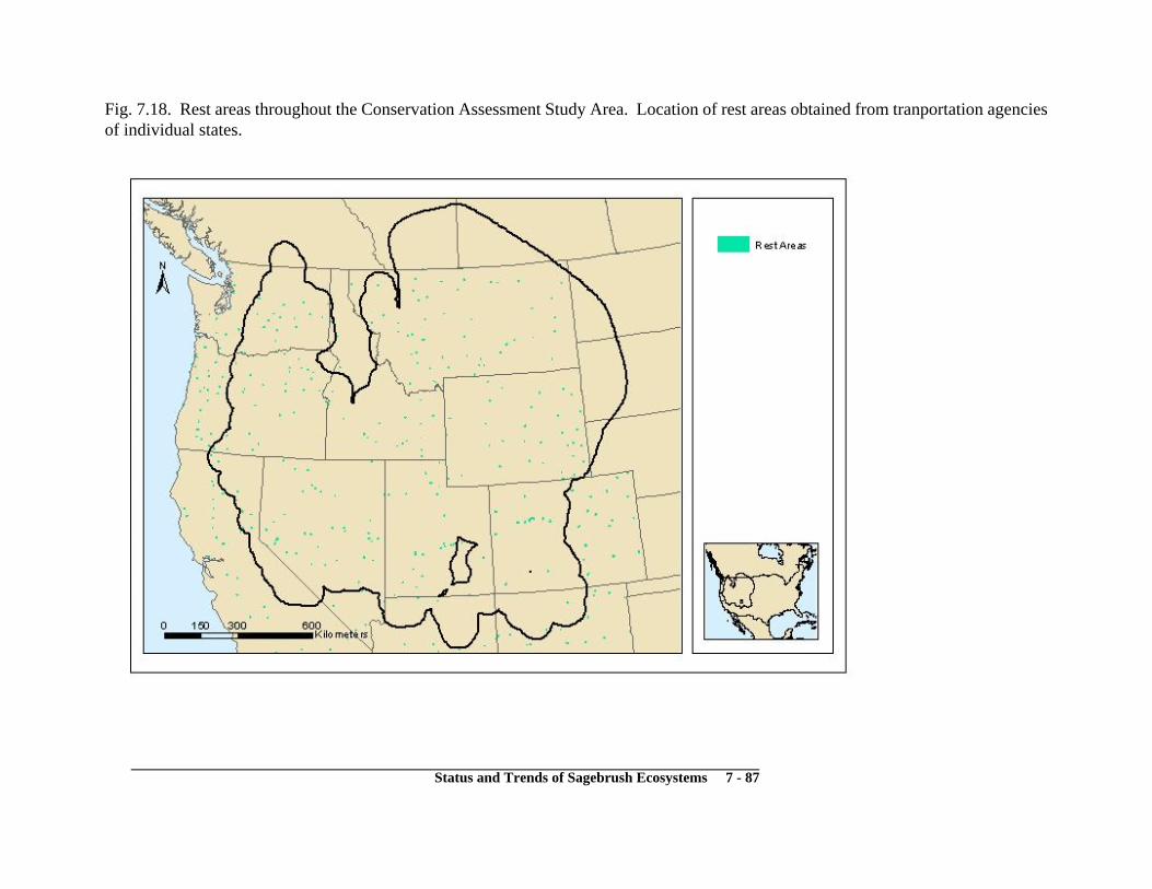
Status and Trends of Sagebrush Ecosystems 7 - 87
Fig. 7.18. Rest areas throughout the Conservation Assessment Study Area. Location of rest areas obtained from tranportation agenciesof individual states.

Status and Trends of Sagebrush Ecosystems 7 - 88
Fig. 7.19. Powerline corridors within the sagebrush biome. (Compiled from 27 GIS coverages obtained from local, state, provincial, andfederal sources).

Status and Trends of Sagebrush Ecosystems 7 - 89
Fig. 7.20. Major railroads in the sagebrush biome. (Data obtained from U.S. National Atlas and Geo Gratis for Canada).

Status and Trends of Sagebrush Ecosystems 7 - 90
Fig. 7.21. Communications towers in the sagebrush biome. (Data obtained from Federal Communication Commission).

Status and Trends of Sagebrush Ecosystems 7 - 91
Fig. 7.22. Linear density of fences on public lands in the Conservation Assessment Study Area. (Compiled from individual GIS coveragesobtained from U.S. Bureau of Land Management District Offices).
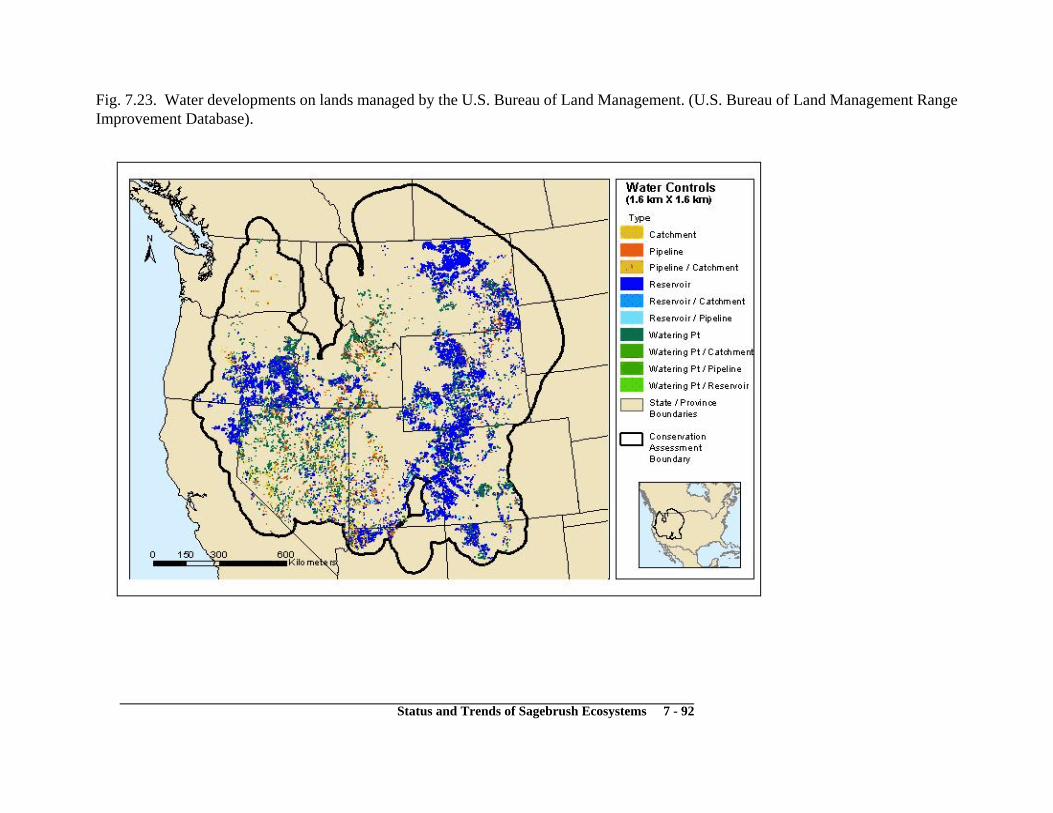
Status and Trends of Sagebrush Ecosystems 7 - 92
Fig. 7.23. Water developments on lands managed by the U.S. Bureau of Land Management. (U.S. Bureau of Land Management RangeImprovement Database).

Status and Trends of Sagebrush Ecosystems 7 - 93
Fig. 7.24. Wild horse management units in the Conservation Assessment Area.

Status and Trends of Sagebrush Ecosystems 7 - 94
Fig. 7.25. Geologic basins in which oil and gas resources have been developed and current distribution of greater sage-grouse. (Compiledfrom 5 state-based Oil and Gas Conservation Commissions, 2 state Geological Surveys, and U.S. Bureau of Land Management).

Status and Trends of Sagebrush Ecosystems 7 - 95
Fig. 7.26. Current producing oil wells in the sagebrush biome. (Compiled from 5 state-based Oil and Gas Conservation Commissions,2 state Geological Surveys, and U.S. Bureau of Land Management).

Status and Trends of Sagebrush Ecosystems 7 - 96
Fig. 7.27. Permitted or pending oil wells in the sagebrush biome (1929-2004). (Compiled from 5 state-based Oil and Gas ConservationCommissions, 2 state Geological Surveys, and U.S. Bureau of Land Management).

Status and Trends of Sagebrush Ecosystems 7 - 97
Fig. 7.28. Current producing gas wells in the sagebrush biome. (Compiled from 5 state-based Oil and Gas Conservation Commissions,2 state Geological Surveys, and U.S. Bureau of Land Management)

Status and Trends of Sagebrush Ecosystems 7 - 98
Fig. 7.29. Permitted or pending natural gas wells in the sagebrush biome (1929-2004). (Compiled from 5 state-based Oil and GasConservation Commissions, 2 state Geological Surveys, and U.S. Bureau of Land Management).

Status and Trends of Sagebrush Ecosystems 7 - 99
Fig. 7.30. Density of primary natural gas and oil pipelines in the Conservation Assessment study area. (Developed fromU.S. Department of Transportation and 17 other sources).

Status and Trends of Sagebrush Ecosystems 7 - 100
Fig. 7.31. Potential for wind energy in the western United States

Status and Trends of Sagebrush Ecosystems 7 - 101
Fig. 7.32. Locations used for military training and testing within the sagebrush biome. (Compiled from U.S. Department of Defense).

Status and Trends of Sagebrush Ecosystems 7 - 102
Fig. 7.33. Conceptual model showing plant dynamics using state and transition (dotted boxes anddashed lines) in a typical shrub grassland site within the sage-grouse range. Solid boxes and arrowswithin states are plant communities and pathways.

Status and Trends of Sagebrush Ecosystems 7 - 103
Table 7.1. Results of univariate linear regressions to detect changes in number and average size offires, total area burned, and variation in fire size by year within floristic divisions from 1980 to2003. The model was a time-series model regressing year by fire variables. Dependent variableswere log-transformed. Dividing by mean fire size standardized variation in within-year fire size.We conducted our analysis only for fires recorded after 1980 because of more consistent reportingeven though fire statistics were available prior to 1980 (Fig. 7.1-5, also 7.6).
Floristic Division(number of fire years 1980 to 2003)
DependentVariable F = P = r2 Coefficient1
Northern Great Basin (23) Fires (n) 91.00 0.01 0.81 0.10Avg. Size (ha) 0.13 0.72 0.04 0.00Total Area (ha) 9.17 0.01 0.27 0.06Variance 2.83 0.11 0.08 -0.04
Southern Great Basin (23) Fires (n) 124.51 0.01 0.85 0.16Avg. Size (ha) 14.83 0.01 0.39 0.09Total Area (ha) 29.86 0.01 0.57 0.16Variance 20.11 0.01 0.46 -0.09
Silver Sagebrush Region (18) Fires (n) 151.10 0.01 0.90 0.33Avg. Size (ha) 0.78 0.39 0.01 0.04Total Area (ha) 74.76 0.01 0.81 0.30Variance 6.73 0.02 0.25 -0.05
Snake River Basin (23) Fires (n) 53.48 0.01 0.70 0.06Avg. Size (ha) 1.20 0.29 0.01 0.01Total Area (ha) 21.88 0.01 0.49 0.05Variance 1.65 0.21 0.03 -0.02
Wyoming Basins (21) Fires (n) 38.98 0.01 0.66 0.26Avg. Size (ha) 5.88 0.03 0.20 0.05Total Area (ha) 41.96 0.01 0.67 0.26Variance 1.69 .0.21 0.03 -0.02
1Log-transformed coefficient
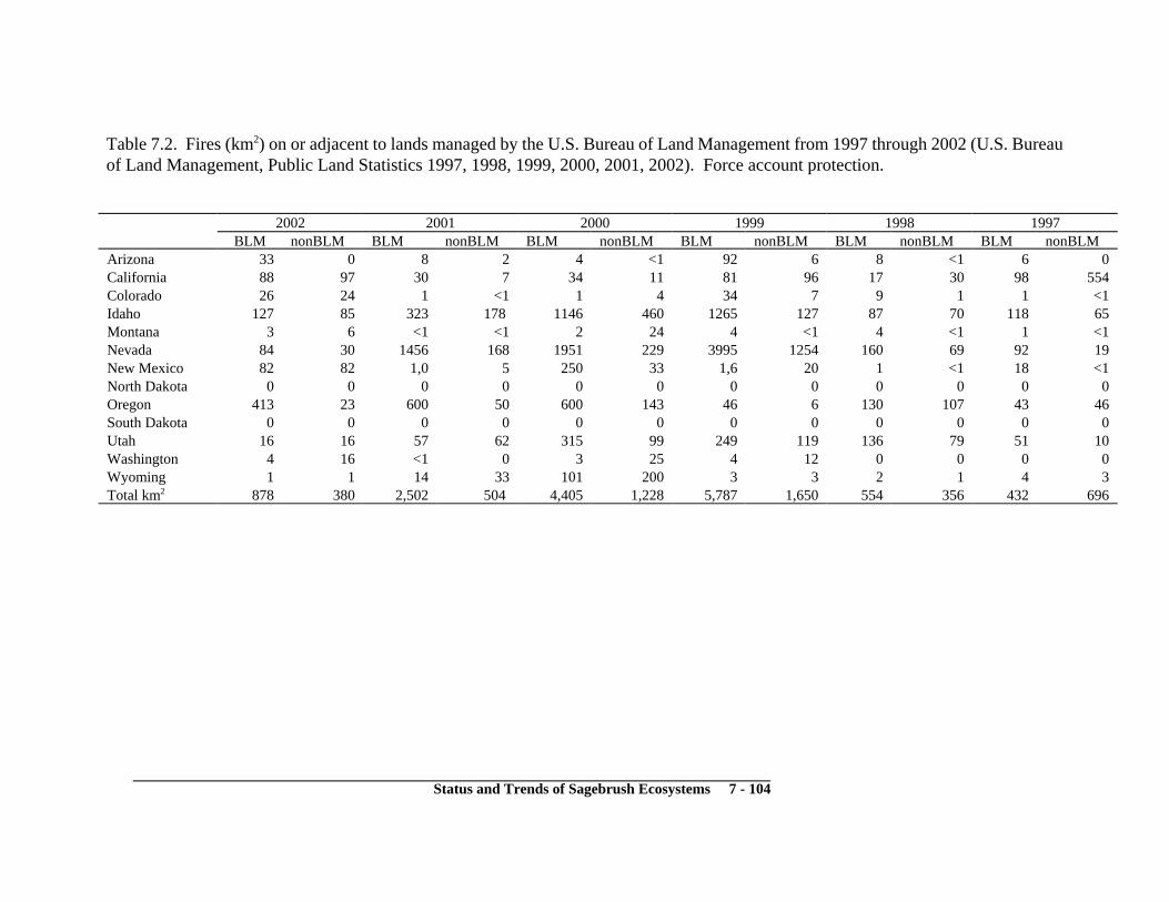
Status and Trends of Sagebrush Ecosystems 7 - 104
Table 7.2. Fires (km2) on or adjacent to lands managed by the U.S. Bureau of Land Management from 1997 through 2002 (U.S. Bureauof Land Management, Public Land Statistics 1997, 1998, 1999, 2000, 2001, 2002). Force account protection.
2002 2001 2000 1999 1998 1997BLM nonBLM BLM nonBLM BLM nonBLM BLM nonBLM BLM nonBLM BLM nonBLM
Arizona 33 0 8 2 4 <1 92 6 8 <1 6 0California 88 97 30 7 34 11 81 96 17 30 98 554Colorado 26 24 1 <1 1 4 34 7 9 1 1 <1Idaho 127 85 323 178 1146 460 1265 127 87 70 118 65Montana 3 6 <1 <1 2 24 4 <1 4 <1 1 <1Nevada 84 30 1456 168 1951 229 3995 1254 160 69 92 19New Mexico 82 82 1,0 5 250 33 1,6 20 1 <1 18 <1North Dakota 0 0 0 0 0 0 0 0 0 0 0 0Oregon 413 23 600 50 600 143 46 6 130 107 43 46South Dakota 0 0 0 0 0 0 0 0 0 0 0 0Utah 16 16 57 62 315 99 249 119 136 79 51 10Washington 4 16 <1 0 3 25 4 12 0 0 0 0Wyoming 1 1 14 33 101 200 3 3 2 1 4 3Total km2 878 380 2,502 504 4,405 1,228 5,787 1,650 554 356 432 696

Status and Trends of Sagebrush Ecosystems 7 - 105
Table 7.3. Fires (km2) on or adjacent to lands managed by the U.S. Bureau of Land Management from 1997 through 2002 (U.S. Bureauof Land Management, Public Land Statistics 1997, 1998, 1999, 2000, 2001, 2002). Contract account protection.
2002 2001 2000 1999 1998 1997BLM nonBLM BLM nonBLM BLM nonBLM BLM nonBLM BLM nonBLM BLM nonBLM
Arizona <1 0 <1 0 <1 <1 0 2 0 1 0 0California 68 106 4 50 99 181 37 73 29 71 53 133Colorado 0 <1 0 <1 0 0 <1 2 1 0 0 0Idaho 9 7 7 13 61 233 20 45 2 227 8 4Montana 4 21 0 <1 2 1 2 2 4 2 0 4Nevada <1 10 1 190 24 84 146 202 7 56 13 9New Mexico <1 1 1 1 7 28 <1 3 4 7 <1 1North Dakota 0 0 0 0 0 0 0 0 0 0 0 0Oregon 1 1 <1 1 3 8 <1 0 29 100 2 24South Dakota 0 0 0 0 0 0 0 0 0 0 0 0Utah 5 15 <1 <1 43 26 47 124 5 1 2 7Washington 8 3 3 5 0 <1 0 0 0 0 0 0Wyoming 1 2 1 22 1 4,8 <1 0 0 <1 1 1Total km2 95 165 16 283 239 609 253 453 80 465 78 178

Status and Trends of Sagebrush Ecosystems 7 - 106
Table 7.4. Characteristics of ecological provinces in the Great Basin Ecoregion and adjacentecoregions (Miller et al. 1999a).
Ecologicalprovince
Precipitation(cm)
pattern
Dominantoverstoryspecies
Old-growth
character
Meanannual
temperature(C)
Elevation(m)
John Day (23 – 46)Winter
Westernjuniper
<3% -2 – 13 1,200 – 2,300
Mazama (18 – 36)Winter
Westernjuniper
>10% 4 – 13 700 – 2,500
Snake River (13 – 31)Winter
-- <3% 4 – 13 900 – 2,000
High Desert (10 – 79)Winter
Westernjuniper
Dense<5%
5 – 10 1,200 – 3,000
Klamath (102 – 305)Winter
-- <3% 7 – 13 460 – 2,800
Humboldt (20 – 76)Winter
Westernjuniper, Utah
juniper
Dense andsavanna
<3%
4 – 10 1,500 – 3,300
Raft River (40 – 100)Winter
Juniper,Singleleaf
pinyon pine
Dense andsavanna
<3%
1 – 9 --
Mono (25 – 64)Winter
Singleleafpinyon pine
Dense<5%
4 – 10 1,200 – 4,300
Lahontan (10 – 30)Winter
Singleleafpinyon pine,Utah juniper
Savanna0%
7 – 13 1,200 – 3,000
Central High (13 – 62)Winter and
summer
Pinyon pine,juniper
Savanna<3%
4 – 10 1,500 – 4,000
HighCalcereous
(13 – 62)Winter and
summer
Juniper,pinyon pine
Savanna<3%
4 – 10 1,500 – 4,000
Bonneville (10 – 25)Winter and
summer
Juniper Savanna>10%
7 – 13 1,200 – 2,400
White River (8 – 51)Winter and
summer
-- Dense andsavanna
11 – 15 1,400 – 2,900

Status and Trends of Sagebrush Ecosystems 7 - 107
Table 7.5. Broad vegetation cover types within the assessment area and their susceptibility to invasion by non-indigenous plant species.Susceptibility to invasion is defined by four categories: (H) high – invades the cover type successfully and becomes dominant orcodominant even in the absence of intense or frequent disturbances; (M) moderate - invades the cover type successfully because highintensity or frequency of disturbance impacts the soil surface or removes the normal canopy cover; (L) low – the species typically doesnot invade the cover type because the cover type does not provide suitable habitat for the species; (U) unknown – distribution records arelimited and interpretation of the susceptibility would be difficult. Compiled from USDA FS and USDI BLM (1997b) and Sheley andPetroff (1999).
Cover Type Invasive Species1
Brte
Canu
Casp.
Cedi
Cema
Cere
Ceso
Cevi
Chju
Chle
Ciar
Civu
Coma
Crvu
Eues
Hagl
Hiau
Hipr
Isti
Lela
Lida
Livu
Lysa
Onac
Pore
Saae
Saka
Seja
Sosp.
Taca
UPLAND COMMUNITIESBasin & Wyoming big & three-tipsagebrush
Artemisia tridentata ssp. tridentata,A.tridentata. ssp. wyomingensis,A. tripartita
H U M M M M M M M U M M L L M M L L H L M M L M U H M U MM
Mountain big sagebrushA. tridentata ssp. vaseyana
HM M M M M M M
M U M M L M L M M L L L H M M L M M M U MM
Low & black sagebrushA. arbuscula, A.nova
M U M M U U M M U U M M L L M M L L H L M U L U U U L U MM
Salt desert shrubAtriplex confertifolia, Eurotia lanata, Grayiaspinosa,Sarcobatus vermiculatus
M M M L L M L M L L M M L L M H L L L L L L L L L L M U M L
Wheatgrass bunchgrassAgropyron sp., Aristida longiseta, Elymuscinereus, Poa secunda, Pseudoroegnariaspicata
H M M H H M H M M M H M L M M M L L H L H M L M H H M U MM
RIPARIAN & WETLANDCOMMUNITIESShrub wetlands M H M M H M M M L M H H H L M L M M M H M M H M M U L U L M

Cover Type Invasive Species1
Brte
Canu
Casp.
Cedi
Cema
Cere
Ceso
Cevi
Chju
Chle
Ciar
Civu
Coma
Crvu
Eues
Hagl
Hiau
Hipr
Isti
Lela
Lida
Livu
Lysa
Onac
Pore
Saae
Saka
Seja
Sosp.
Taca
Status and Trends of Sagebrush Ecosystems 7 - 108
Cornus sp., Salix sp.
Cottonwood Populus trichocarpa
M M M M H M M M M H H M H L H L M H M H M M M M M M L U LM
Herbaceous WetlandCarex nebraskensis, C. rostrata, C. aquatilis
M M M M H M H M L H H M H L M L H M M H M M H H M H L U LM
1Brte Bromus tectorum (cheatgrass); Canu Carduus nutans (musk thistle); Ca sp. Cardaria species (whitetop); Cedi Centaurea diffusa (diffuse knapweed); Cema Centaurea maculosa (spotted knapweed);Cere Centaurea repens (Russian knapweed); Ceso Centaurea solstitialis (yellow starthistle); Cevi Centaurea virgata (squarrose knapweed); Chju Chondrilla juncea (Rush skeletonweed); Chle Chrysanthemumleucanthemum (Oxeye daisy); Ciar Cirsium arvense (Canada thistle); Civu Cirsium vulgare (bull thistle); Coma Conium maculatum (poison-hemlock); Crvu Crupina vulgaris (common crupina); EuesEuphorbia esula (leafy spurge); Hagl Halogeton glomeratus (halogeton); Hiau Hieracium aurantiacum (orange hawkweed); Hipr Hieracium pratensis (meadow hawkweed); Isti Isatic tinctoria (dyer’s woad);Lela Lepidium latifolium (perennial pepperweed); Lida Linaria dalmatica (Dalmation toadflax); Livu Linaria vulgaris (yellow toadflax); Lysa Lythrum salicaria (purple loosestrife); Onac Onopordumacanthium (Scotch thistle); Pore Potentilla recta (sulphur cinquefoil); Saae Salvia aethiopis (Mediterranean sage); Saka Salsola kali (Russian thistle); Seja Senecio jacobaea (tansy ragwort); So sp. Sonchussp. (sowthistles); taca Taeniatherum caput-medusae (medusahead)

Status and Trends of Sagebrush Ecosystems 7 - 109
Table. 7.6. Mean population density (in millions) within states from U.S. Census Statistics from 1900 to 2000.
Year of United States CensusState 2000 1990 1980 1970 1960 1950 1940 1930 1920 1910 1900
Arizona 3.26 2.46 1.90 1.18 0.91 0.71 0.62 0.47 0.36 0.26 0.21California 17.70 14.56 10.71 7.46 6.05 4.88 3.72 2.75 2.34 2.32 2.21Colorado 16.06 12.59 10.93 7.47 5.11 3.75 3.38 2.86 2.69 3.02 2.89Idaho 10.84 8.31 7.72 5.76 5.36 4.82 4.22 3.58 3.43 4.12 2.12Montana 2.60 2.33 2.36 2.17 2.19 1.99 1.93 1.94 2.14 2.77 2.44North Dakota 1.49 1.60 1.73 1.64 1.81 1.76 1.85 2.17 2.02 2.15 0.93Nebrasaka 4.18 4.18 4.48 4.23 4.30 4.16 4.11 3.94 3.06 1.79 1.04New Mexico 11.77 10.43 10.10 8.25 7.25 6.00 2.43 1.94 1.77 1.63 1.57Nevada 14.95 10.41 7.70 3.98 2.21 1.23 0.98 0.73 0.79 1.22 1.10Oregon 36.75 31.69 30.06 27.44 24.92 22.18 16.58 15.41 12.67 11.55 6.03South Dakota 2.74 2.54 2.40 2.09 2.11 1.84 1.79 1.67 1.39 2.10 1.98Utah 29.38 23.15 19.59 14.50 11.96 8.76 6.66 6.12 5.24 4.71 3.26Washington 30.06 25.48 22.28 19.16 16.51 13.65 9.74 8.89 8.02 7.19 3.61Wyoming 2.17 1.99 2.01 1.48 1.52 1.35 1.18 1.07 1.03 1.16 0.79

Status and Trends of Sagebrush Ecosystems 7 - 110
Table. 7.7. Recreational use (number of visitors and visitor days) on lands managed by the U.S. Bureau of Land Management (U.S. Bureauof Land Management, Public Land Statistics 2000, 2001, 2002). Number of visitors represents the total of recreational visits to all lands,including those managed specifically for recreation or other opportunities. Number of visitor-days is an aggregate of 12 visitor-hours toa site or area.
2002 2001 2000Visitors Visitor Days Visitors Visitor Days Visitors Visitor Days
Arizona1 1,778 4,393 4,572 14,102 4,997 15,515California 8,947 16,747 8,312 13,684 8,400 10,610Colorado 4,440 3,394 4,892 3,410 4,756 3,206Idaho 6,090 4,710 5,895 4,296 6,326 4,513Montana 2,845 2,459 2,955 3,405 3,136 3,523Nevada 6,438 5,184 5,275 3,606 5,045 4,110New Mexico 2,090 1,788 2,533 1,800 2,380 1,667Oregon 7,635 6,511 8,265 7,220 8,137 9,200Utah 5,733 7,757 5,795 7,055 6,169 7,812Wyoming 2,022 2,282 1,931 2,043 3,655 2,285Total 48,018 55,225 50,425 60,621 53,001 62,441
1Does not include 2,905 visitors and 10,036 visitor days to leased or partnership sites that previously were included in previous year’stotals.

Status and Trends of Sagebrush Ecosystems 7 - 111
Table 7.8. Number of habitat treatments on lands managed by the U.S. Bureau of Land Management (U.S. Bureau of Land ManagementRange Improvement Projects database).
StateHabitat Treatment AZ CA CO ID MT ND NM NV OR SD UT WA WY Total
Unknown 9 20 15 23 30 12 40 18 91 25 283Fences 1,489 669 3,051 3,717 5,790 48 1,445 3,489 3,451 357 3,265 239 5,278 32,288Fence modification 1 6 9 149 17 7 23 89 17 4 23 345Hazard reduction 1 8 28 47 9 1 5 10 2 4 115Land treatment 30 15 253 158 82 78 77 54 4 141 11 73 976Lake/wetland improvement 21 8 8 17 2 7 1 2 10 8 84Misc. facility improvement 468 173 1,038 1,254 1,420 368 1,480 1,263 10 1,300 41 644 9,459Perch/nesting structure 2 6 7 2 3 3 6 11 44 84Stream improvement 8 35 11 13 3 1 14 17 4 22 128Streambank stabilization structures 1 18 4 13 1 2 11 1 3 2 56Timber stand improvement 8 23 9 1 3 1 15 1 1 12 74Vegetation manipulation 220 207 880 1,585 445 9 681 895 1,089 14 824 66 481 7,396Weed control 2 138 67 320 3 31 12 126 15 14 294 42 1,064Water development/control 2,180 1,180 9,189 5,017 10,587 56 2,247 5,163 7,555 561 5,292 130 7,813 56,970Water facilities modified 15 49 65 15 3 3 126 1 20 2 38 337Total habitat treatments 4,420 2,311 14,736 12,120 18,766 116 4,884 11,194 13,831 963 10,995 816 14,509 109,661

Status and Trends of Sagebrush Ecosystems 7 - 112
Table 7.9. Summary of Grazing Permits and Leases in Force on Public Lands from 2000 through 2002 (U.S. Bureau of Land Management,Public Land Statistics 2000, 2001, 2002)
2002 2001 2000Permits AUMs Permits AUMs Permits AUMs
Arizona 741 685,257 767 676,970 785 678,962California 627 328,404 593 316,971 603 329,395Colorado 1,627 648,693 1,609 644,603 1,639 691,046Idaho 1,959 1,322,974 1,939 1,317,041 1,962 1,323,215Montana 3,787 1,293,498 3,755 1,286,197 3,832 1,302,641Nebraska 20 622 18 592 21 622Nevada 658 2,241,596 661 2,221,140 683 2,225,814New Mexico 2,313 1,875,361 2,312 1,872,958 2,321 1,875,181North Dakota 75 9,389 75 9,389 74 9,379Oklahoma 4 138 4 138 4 138Oregon 1,395 1,059,047 1,296 1,036,769 1,359 1,041,707South Dakota 462 74,126 466 74,387 456 73,448Utah 1,569 1,234,136 1,550 1,236,840 1,589 1,246,639Washington 363 29,475 324 30,536 298 28,239Wyoming 2,782 1,973,653 2,773 1,972,836 2,767 1,984,061Total 18,382 12,776,369 18,142 12,697,367 18,393 12,810,487

Status and Trends of Sagebrush Ecosystems 7 - 113
Table 7.10. Percent of lands by seral condition on public lands managed by the U.S. Bureau of Land Management in 2003a,b. Potentialnatural climax = 76-100% similar; late seral = 51-75% similar; mid-seral = 26-50% similar; early seral = 0-25% similarc.
%Inventoried
PotentialNatural
CommunityLateSeral
Mid-Seral
Early-Seral Unclassified
Arizona 76 6 32 26 7 30California 16 3 20 43 30 4Colorado 58 5 20 40 18 27Idaho 54 3 27 38 27 5Montana,North Dakota,South Dakota 78 7 58 21 1 13Nevada 54 3 27 31 8 31New Mexico 80 4 30 41 22 3Oregon andWashington 82 1 21 45 11 23Utah 62 11 28 42 13 6Wyoming 56 24 34 27 5 10Total 61 7 29 34 11 18
ahttp://www-a.blm.gov/natacq/pls03/bStatistics are reported for 2003 although surveys to classify sites may have been conducted in other years.cA common qualitative characterization of plant communities is for potential natural communities to be considered as in “excellentcondition”, late seral stages to be “good”, mid-seral to be “fair”, and early seral to be “poor”. Because these terms may not accuratedescribe current understanding of succession dynamics in sagebrush ecosystems (West 2003), the U.S. Bureau of Land Management isconsidering changes to standards and guidelines that indicate “rangeland health” (U.S. Bureau of Land Management 2003b) (Table 7.11).

Status and Trends of Sagebrush Ecosystems 7 - 114
Table 7.11. Total area (km2 and %) of lands managed by the U.S. Bureau of Land Management meeting standards and guidelinesestablished for rangeland health1. Category A = meeting standards or making significant progress towards meeting standards. CategoryB = Not meeting all standards or making significant progress but appropriate action has been taken to ensure significant progress towardsmeeting standards (livestock is a significant factor). Category C = Not meeting standards or making significant progress towards meetingthe standards and no appropriate action has been taken to ensure significant progress (livestock is a significant factor). Category D = Notmeeting standards or making significant progress towards meeting the standards due to causes other than livestock grazing. Category E= total area assessed. Category F = total area that has not been assessed.
Category A Category B Category C Category D Category E Category Fkm2 % km2 % km2 % km2 % km2 % km2 % Total
Arizona 20,264 42 1,434 3 859 2 109 0 22,667 47 25,605 53 48,272California 12,287 39 2,637 8 1,477 5 2,078 7 18,479 58 13,392 42 31,870Colorado 14,588 41 5,787 16 99 0 1,404 4 21,878 62 13,597 38 35,475Idaho 8,384 18 12,575 26 1,826 4 2,525 5 25,310 53 22,449 47 47,760Montana/Dakotas 19,745 60 1,919 6 599 2 661 2 22,924 70 10,032 30 32,957Nevada 25,914 14 39,174 21 2,720 1 4,167 2 71,975 39 113,035 61 185,010New Mexico 1,466 3 374 1 0 0 24 0 1,864 4 48,529 96 50,392Oregon/Washington 12,904 23 4,335 8 2,044 4 1,133 2 20,416 36 35,835 64 56,251Utah 19,487 21 4,640 5 1,052 1 5,016 6 30,194 33 60,722 67 90,917Wyoming 25,592 35 14,278 20 2,654 4 778 1 43,303 60 29,074 40 72,377Total 160,629 25 87,154 13 13,331 2 17,897 3 279,011 43 372,270 57 651,2811www.blm.gov/nstc/rangeland/rangelandindex.html

Status and Trends of Sagebrush Ecosystems 7 - 115
Table 7.12. Total area (km2) seeded on lands managed by the U.S. Bureau of Land Management for wildlife habitat improvement (U.S.Bureau of Land Management, Public Land Statistics 1997, 1998, 1999, 2000, 2001, 2002).
YearState 2002 2001 2000 1999 1998 1997
Arizona 1 <1 57 1 0 16California 0 1 0 <1 5 4Colorado 25 21 3 1 1 <1Idaho 0 0 0 4 0 283Montana <1 8 0 2 1 3Nevada 265 202 1,582 90 45 23New Mexico <1 1 2 6 0 <1North Dakota 0 0 0 0 0 0Oregon 0 93 20 1 3 6South Dakota 0 0 0 0 0 0Utah 14 0 7 67 0 74Washington 0 0 0 0 0 0Wyoming 1 12 2 <1 0 0Total area (km2) 306 339 1,673 173 55 410

Status and Trends of Sagebrush Ecosystems 7 - 116
Table 7.13. Total area (km2) treated with disking and chaining for wildlife improvements on lands managed by the U.S. Bureau of LandManagement from 1997 through 2002. (U.S. Bureau of Land Management, Public Land Statistics 1997, 1998, 1999, 2000, 2001, 2002).
YearState 2002 2001 2000 1999 1998 1997
Arizona <1 0 2 1 <1 1California 0 0 0 0 <1 <1Colorado 37 0 <1 <1 1 1Idaho 0 0 0 0 0 0Montana 0 0 0 1 1 3Nevada 13 0 8 0 3 0New Mexico 3 1 13 9 0 <1North Dakota 0 0 0 0 0 0Oregon 0 10 1 <1 4 3South Dakota 0 0 0 0 0 0Utah 23 0 4 9 0 190Washington 0 0 0 0 0 0Wyoming 1 5 0 2 0 23Total area (km2) 77 16 29 23 9 221

Status and Trends of Sagebrush Ecosystems 7 - 117
Table 7.14. Total area (km2) treated by prescribed fire projects on lands managed by the U.S. Bureau of Management from 1997 to 2002.(U.S. Bureau of Land Management, Public Land Statistics 1997, 1998, 1999, 2000, 2001, 2002)
YearState 2002 2001 2000 1999 1998 1997
Arizona 52 48 40 94 95 8California 7 3 22 21 45 16Colorado 24 2 2 46 56 3Idaho 59 100 43 102 64 11Montana 12 34 15 31 18 3Nevada 28 10 <1 3 2 10New Mexico 53 34 15 71 131 60North Dakota 0 0 0 0 0 0Oregon 223 86 55 225 169 72South Dakota 0 0 0 0 0 0Utah 19 64 33 30 24 11Washington 0 0 4 1 0 0Wyoming 20 11 23 138 117 59Total area (km2) 497 393 251 764 720 253

Status and Trends of Sagebrush Ecosystems 7 - 118
Table 7.15. Nonfire fuels treatment (km2) on lands managed by the U.S. Bureau of Land Management (U.S. Bureau of Land Management.Public Land Statistics1999, 2000, 2001, 20002). Includes mechanical (e.g, chaining), hand (e.g., thinning and pulling), and chemical (e.g.,herbicide) treatments.
YearState 2002 2001 2000 1999
Arizona 46 32 10 <1California 14 4 5 7Colorado 60 74 9 15Idaho 228 324 277 20Montana 15 0 <1 0Nevada 40 6 123 0New Mexico 150 4 5 4North Dakota 0 0 0 0Oregon 160 55 27 6South Dakota 0 0 0 0Utah 63 0 1 14Washington 1 1 0 0Wyoming 54 52 2 0Total area (km2) 832 553 460 66

Status and Trends of Sagebrush Ecosystems 7 - 119
Table 7.16. Number of projects (n), total area (km2) treated, and funding (USD) approved for emergency fire rehabilitation on landsmanaged by the U.S. Bureau of Land Management from 1997 through 2002 (U.S. Bureau of Land Management, Public Land Statistics1997, 1998, 1999, 2000, 2001, 2002).
Year2002 2001 2000 1999 1998 1997
State n km2 Funding ($) n km2 Funding ($) n km2 Funding ($) n km2 Funding ($) n km2 Funding ($) n km2 Funding ($)Arizona 1 67 1,021,000 0 0California 19 34 574,591 6 2,3 1,647,405 7 168 1,148,647 5 11 18,154,000 0 0Colorado 16 52 2,816,202 4 2,3 167,484 15 77 1,094,737 5 45 295,000 9 6 93,859 0Idaho 85 2,900 2,292,252 31 389 4,577,439 38 1,216 10,605,954 41 1,267 7,802,576 8 53 410,379 14 45 473,195Montana 3 8 1,064,471 0 0 5 65 461,000 0 0 0Nevada 103 11,226 17,061,510 74 1,570 23,475,497 41 1,924 24,371,902 40 4,696 44,102,482 7 81 1,367,045 14 204 1,734,644New Mexico 0 0 0 0 0 0North Dakota 0 0 0 0 0 0Oregon 50 1,392 4,794,421 22 856 6,656,000 9 450 4,841,000 10 48 655,000 7 94 880,000 0South Dakota 0 0 0 0 0 0Utah 27 409 2,309,559 29 65 1,969,000 32 262 8,111,398 20 188 6,050,054 21 121 2,577,474 7 32 439,300Washington 0 0 0 0 0 0Wyoming 5 113 423,125 1 2 590,300 8 460 1,353,671 1 1 49,315 0 0Total 308 16,135 31,336,131 167 2,927 39,083,125 155 4,621 51,988,309 123 6,324 78,129,427 52 341 5,328,757 35 281 2,647,139

Status and Trends of Sagebrush Ecosystems 7 - 120
Table 7.17. Estimates of numbers of free-roaming horses and burros on lands administered by the U.S. Bureau of Land Management inthe western United States in 2003, and the sum of Appropriate Management Levels [AMLs] (summed across all Herd Management Areas[HMAs] in the state). AML is determined through a multiple-use process, in which animal-unit months (AUMs) are distributed amongfree-roaming equids, livestock, and native ungulates. Estimated population sizes do not include animals occurring on other publicjurisdictions.
Horses Burros Total Equid
State Population AML Population AML Population
Arizona 250 210 2,243 1,580 2,493
California 2,607 1,733 810 416 3,417
Colorado 516 812 0 0 516
Idaho 697 999 0 0 697
Montana 170 105 0 0 170
Nevada 16,857 13,648 919 976 17,776
New Mexico 68 50 0 0 68
Oregon 2,870 2,615 15 25 2,885
Utah 2,155 1,835 126 120 2,281
Wyoming 5,035 3,725 0 0 5,035
Total 31,225 25,732 4,113 3,117 38,815

Status and Trends of Sagebrush Ecosystems 7 - 121
Table 7.18. Number of applications for oil and gas leases received by federal agenciesa from 1929to 2004. (Data obtained from U.S. Bureau of Land Management LR2000 Lands and Recordsdatabase).
Number of leasesState Authorized Pending Rejected Withdrawn Total
Wyoming 50,852 606 61 1,098 52,617Arizona 128 7 0 0 135California 1,510 134 4 104 1,752Colorado 13,498 308 8 102 13,916Idaho 16 0 0 0 16Montana 10,180 1,360 4 48 11,592New Mexico 25,695 140 4 84 25,923Nevada 2,272 201 20 8 2,501Oregon 73 9 0 0 82Washington 500 0 0 0 500Utah 8,475 362 2 42 8,881South Dakota 467 100 0 2 569North Dakota 3,568 440 0 4 4,012Total (%) 117,234 (95.7) 3,667 (3.0) 103 (0.1) 1,492 (1.2) 122,496aPrior to 1972, the U.S. Geological Survey was the approval authority for applications for permit todrill. The U.S. Bureau of Land Management was authorized to provide input into the decisionprocess in 1972 and became the approving authority in 1982 following a merger with the MineralsManagement Service.

Status and Trends of Sagebrush Ecosystems 7 - 122
Table 7.19. Geologic basins (Fig. 7.25) where significant oil and gas resources have been developedwithin the sagebrush biome, total area (km2), and area (km2) of sagebrush included within the basin.(Data obtained from U.S. Geological Survey National Oil and Gas Assessment).
Basin Name State(s) Total Area(km2)
Sagebrush Area(km2)
1. Greater GreenRiver Basin
Wyoming, Colorado,Utah
114,137 49,118
2. Powder RiverBasin
Wyoming, Montana 89,178 21,061
3. Uinta-PiceanceBasin
Utah, Colorado 78,493 13,393
4. Wyoming ThrustBelt
Wyoming, Utah, Idaho 29,211 11,934
5. Paradox - San JuanBasin
Utah 158,779 18,498
Wind River Basin Wyoming 30,312 15,787Bighorn Basin Wyoming, Montana 34,087 10,567Williston Basin Montana, North
Dakota, South Dakota89,178 9,442
North-CentralMontana
Montana 123,102 6,273

Status and Trends of Sagebrush Ecosystems 7 - 123
Table 7.20. Major category of stipulations on oil/gas development, total area (km2) and percent offederal lands affected in five major and priority geological basins (adapted from Table ES-1; U.S.Departments of the Interior, Agriculture and Energy 2003)
Access Category Area (km2) Federal Lands (%)No Leasing (Statutory/Executive Order) 40,745 16.9No Leasing (Administrative) pending NEPAor LUP action. 24,310 10.1No Leasing (Administrative), general 20,632 8.6Leasing, no surface occupancy 10,984 4.6Leasing, cumulative timing limitations ondrilling >9 months 101 0Leasing, cumulative timing limitations ondrilling 6-9 months 10,202 4.2Leasing, cumulative timing limitations ondrilling 3-6 months 22,024 9.2Leasing, cumulative timing limitations ondrilling <3 months 2,821 1.2Leasing, controlled surface use 15,188 6.3Leasing, standard lease terms 93,449 38.9

Status and Trends of Sagebrush Ecosystems 7 - 124
Table 7.21. Area (km2) of major oil and gas producing fields and number of wells and spacing(ha/well) for the Greater Green River Basin, Wyoming (Fig. 7.25). (Compiled from U.S. GeologicalSurvey National Oil and Gas Assessment and U.S. Bureau of Land Management state and fieldoffice personnel).
Name of Field/AreaArea(km2)
Number of wells Spacing (ha/well)Approve
d Drilled PotentialCurrentRange Potential
Continental Divide(many fields)
4,293 2,100 3,000 32-65 32
Jonah II 241 497 497 16-32 16Jonah II+ (proposed addition) no final proposal to date
118 Proposedbut not
approved
3,100additional
wells
2-16 2-16
Pinedale Anticline 638 900 900 16-65 8-65Big/Piney LaBarge per CAP 797 No limit No limit 4-16 4-16Moxa Arch 1,930 .1,500 .2,200 65 UnknownFontenelle 725Blue Gap 81 65 UnknownGreat Divide Field, Colorado 16 16Big Hole Field, Colorado 16 16Little Snake Field Office,Colorado
497 2,327 1,979 3,327 16-130 8

Status and Trends of Sagebrush Ecosystems 7 - 125
Table 7.30. Area (km2) of major oil and gas producing fields and number of wells and spacing forthe Powder River Basin, Wyoming and Montana (Fig. 7.25). Area was determined from individualEnvironmental Impact Statements or mapped estimates. (Compiled from U.S. Geological SurveyNational Oil and Gas Assessment and U.S. Bureau of Land Management state and field officepersonnel).
Name of Field/AreaArea(km2)
Number of wells Spacing (ha/well)Approved Drilled Potential Range Potential
Powder River Basin, Wyoming(Coalbed Methane)
32,376 15,300 .15,000 51,000 32 32
Powder River Basin, Montana(Coalbed Methane)
11,028 511 480 15,635 32 32
Salt Creek and Teapot Dome 1,600 4-16 4-16Sand Dunes Field 30-40 16 16Fina/Fly Draw/Phillips Cr. 30-40 65 65
Table 7.31. Area (km2) of major oil and gas producing fields, number of wells and spacing (ha/well)for the Uinta/Piceance Basin in Utah and Colorado (Fig. 7.25). Area was determined fromindividual Environmental Impact Statements (EIS), Environmental Assessments (EA) or mappedestimates. (Compiled from U.S. Geological Survey National Oil and Gas Assessment and U.S.Bureau of Land Management state and field office personnel).
Name of Field/AreaArea(km2)
Number of wells SpacingApproved Drilled Potential Range Potential
Red Wash/Greater DeadmanBench
595 New EIS inprogress
1,464 1,249 16-65 16
Natural Buttes 316 875 - EA 704 171 16-32 16Castlegate CBM 103 154 - EIS 30 124 65 16-32Myton Bench 265 New EIS in
Progress714 933 16-32 16
Prickly Pear 265 160 - EA 40 120 65 16-32Altamont-Bluebell 1396 549 Unk 16-65 16

Chapter 8
Greater Sage-Grouse Genetics

Greater Sage-Grouse Genetics 8 - 1
CHAPTER 8
Greater Sage-grouse Genetics
Abstract. Recent research on greater sage-grouse (Centrocercus urophasianus) genetics has helped identify some important characteristics. First, the greater sage-grouse is genetically distinct from the congeneric Gunnison sage-grouse (C. minimus). Second, the Mono Lake area of California (but also Washington to a lesser extent), appears to have some unique genetic characteristics. Third, the previous delineation of western (C. u. phaios) and eastern (C. u. urophasianus) subspecies was not supported. Fourth, the two isolated populations in Washington are showing indications that genetic heterogeneity has been lost due to population declines and isolation. Additional work is being planned and conducted that will help address unanswered questions.
Introduction
Genetic techniques have only recently begun to be used in studies of wildlife. With
recent technological advances, straightforward and rather inexpensive genetic techniques have emerged which can be directly applied to wildlife studies. Genetic techniques are currently being used to investigate relationships among species, populations, family groups, and individuals.
Genetic studies all examine portions of DNA at some scale. Two different genomes are used in genetic studies of animals. The nuclear genome is biparentally inherited and is found in the cell nucleus. It is large and not well mapped in most species. The mitochondrial genome is housed in the mitochondrion, an organelle involved in cellular metabolism. It is small compared to the nuclear genome and is a circular, maternally inherited molecule that has been well mapped in many species. Nuclear DNA on average evolves slowly, although some portions (e.g., microsatellites) evolve quickly. Mitochondrial DNA (mtDNA) on average evolves more quickly than the nuclear genome and some areas (e.g., control region) evolve very rapidly. These features make mtDNA and some regions of nuclear DNA suitable targets for certain genetic studies (Avise 1994).
Since it is virtually impossible to look at the entire genome, we typically target different
areas throughout the genome to use in analyses. These “targeted” areas are called molecular markers. Because different stretches of DNA evolve (or mutate) at different rates, one can address different questions by targeting different regions of the genome. Systematic relationships are often investigated using the more slowly evolving cytochrome-B gene of the mtDNA whereas population genetic studies often target the hypervariable control region of mtDNA.
Published genetic studies of greater sage-grouse have focused on several questions. A
number of authors have investigated the phylogenetic relationship of greater sage-grouse to other grouse species (Ellsworth et al. 1996, Gutierrez et al. 2000, and Drovetski 2002). These studies will not be described here as their focus is on evolutionary relationships among species rather than relationships within the greater sage-grouse. One study investigated the mating system of greater sage-grouse by comparing behavioral data and genetic data (Semple et al. 2001). Three

Conservation Assessment of Greater Sage-grouse and Sagebrush Habitats Connelly et al.
Greater Sage-Grouse Genetics 8 - 2
other studies have looked at taxonomic boundaries and population genetics (Kahn et al. 1999, Oyler-McCance et al. 1999, and Benedict et al. 2003).
Investigating the Lek Mating System Behavioral aspects of the lek mating system of greater sage-grouse have been studied (Wiley 1973, Gibson and Bradbury 1986, Gibson et al. 1991) and suggest that few males do most of the mating and that females typically only mate with one dominant male. There is some evidence, however, to suggest that there exists a component to the mating system that was unobserved by previous studies whereby females may be mating off the lek with purportedly non-dominant males. To investigate this issue, Semple et al. (2001) used six hypervariable microsatellite markers to identify the parentage of 10 broods of greater sage-grouse in Long Valley, California.
In this study, Semple et al. (2001) made behavioral observations on attendance, territoriality and mating behavior of males on one lek. Each male was uniquely identified using colored leg bands. Both males and females associated with this lek were trapped and blood samples collected. Females were radio-collared and followed throughout the breeding process. After 7 – 9 days of incubation, nests were located and all eggs were collected and embryos were sacrificed for genetic analysis.
Six variable microsatellite loci were used to identify the parentage of all embryos. The genotypes of the embryos were compared to the associated mother to identify which alleles were maternal and which were paternal. The number of paternal alleles was then used to determine whether the brood had been sired by more than one male. An attempt was made to exclude potential males as fathers based on their microsatellite genotypes.
Semple et al. (2001) found that all broods had genotypes consistent with their putative mother and that eight of ten broods showed results consistent with only one father. Two broods did show results suggesting that at least two males had fathered the brood. Of the ten females with broods, only four mated on the lek from which behavioral observations were made and thus were seen copulating. Three of those four females mated with males that had been genotyped and in each case the putative father could not be excluded as the father based on genotype data. The fourth female mated with a male who was not banded or genotyped. Therefore, Semple et al. (2001) concluded that in all four cases, the genetic data were consistent with behavioral data. While previous studies suggested very low instances of multiple paternity, this study showed that it may be more prevalent than was once thought.
Population Genetics of Sage-grouse in Colorado Two published studies have investigated population genetic structure in Colorado (Kahn et al. 1999, Oyler-McCance et al. 1999). These two studies were initiated after morphological (Hupp and Braun 1991) and behavioral (Young et al. 1994) evidence suggested the sage-grouse in southwestern Colorado and southeastern Utah were different from sage-grouse elsewhere. The goal of the two genetic studies was to determine whether there were genetic differences between sage-grouse from Southwestern Colorado and those from Northwestern Colorado.

Conservation Assessment of Greater Sage-grouse and Sagebrush Habitats Connelly et al.
Greater Sage-Grouse Genetics 8 - 3
Kahn et al. (1999) sequenced 141 base pairs of the rapidly evolving control region of
mtDNA from approximately 20 individuals each from seven populations. Six of those populations were the larger-bodied greater sage-grouse sampled from Eagle, North Park, Cold Springs, Middle Park, and Blue Mountain in Colorado and from Rich County in Utah. The remaining population was the smaller-bodied yet to be described Gunnison sage-grouse sampled from the Gunnison Basin. All DNA samples were extracted from muscle tissue obtained from hunter-killed sage-grouse.
This study revealed that all the greater sage-grouse populations had many mtDNA haplotypes present per population (average of 7.3 haplotypes per population) while the Gunnison sage-grouse population had only 2 haplotypes present. The greater sage-grouse populations were dominated by four haplotypes (Table 8.1) A, B, C, and D. The Gunnison sage-grouse population had only one of those four haplotypes (A) and had a haplotype G, which was unique to the Gunnison sage-grouse. Kahn et al. (1999) noted the dramatically different haplotype frequencies between the Gunnison sage-grouse and the greater sage-grouse. They performed a maximum parsimony analysis on the haplotype sequences using a heuristic search algorithm and constructed a phylogram (Fig. 8.1). This analysis revealed that all haplotypes fell into one of two deep clades. All populations of greater sage-grouse had individuals from both clades. They suggest that the two deep clades began diverging at least 850,000 years ago during the Pleistocene. Under this hypothesis the two clades subsequently intermixed as these populations re-converged.
Oyler-McCance et al. (1999) expanded on the study by Kahn et al. (1999) by including data from four nuclear microsatellites and also adding approximately 20 samples each from three additional populations of Gunnsion sage-grouse (Crawford, Dry Creek Basin, and Dove Creek). Their additional samples were DNA extracted from blood taken from trapped Gunnison sage-grouse.
This study showed similar results to those found by Kahn et al. (1999) in that the greater sage-grouse showed much more genetic diversity in mitochondrial haplotypes with an average of 7.3 haplotypes per population compared to an average of 2.3 haplotypes per population among the four populations of Gunnison sage-grouse. Further, the microsatellite data is concordant with this pattern with higher levels of allelic diversity among the greater sage-grouse (average of 5.7 alleles per locus) than among the Gunnison sage-grouse (average of 2.6 alleles per locus). Population genetic analysis revealed a lack of evidence of gene flow among the two groups of sage-grouse (Fig. 8.2) which is consistent with the idea that the Gunnison sage-grouse should be recognized as a new species (Young et al. 2000). Further, Oyler-McCance et al. (1999) showed that there was much less gene flow among populations of Gunnison sage-grouse (FST = 0.0266, 95% CI 0.0016-0.0528) than among populations of greater sage-grouse (FST = 0.2153, 95% CI 0.1230-0.3339).

Conservation Assessment of Greater Sage-grouse and Sagebrush Habitats Connelly et al.
Greater Sage-Grouse Genetics 8 - 4
Evaluation of the Eastern & Western Subspecies
Historically, sage-grouse were classified into two subspecies: eastern (C. u. urophasianus) and western sage-grouse (C. u. phaios) based on plumage and coloration differences in eight individuals collected from Washington, Oregon and California (Aldrich 1946). Western sage-grouse presumably occurred in southern British Columbia, central Washington, east-central Oregon, and northeastern California (Aldrich 1946). Populations in other areas of the range are considered to be eastern sage-grouse. The validity of this taxonomic distinction has since been questioned (Johnsgard 1983). While this species has recently been the target of extensive conservation efforts, the taxonomic/genetic relationships between populations/subspecies remain poorly understood. Because the distinction between the eastern and western subspecies has been questioned (Johnsgard 1983), Benedict et al. (2003) investigated whether there was evidence at the genetic level to support it. While genetic data alone can neither prove nor disprove a subspecies distinction, Benedict et al. (2003) surmise, as does Young et al. (2000), that morphological, behavioral and genetic data when used in conjunction, can help clarify such taxonomic questions. In addition, Benedict et al. (2003) were interested in providing information relevant to an understanding of gene flow, genetic diversity and evolutionary history between sage-grouse populations in Washington, Oregon, Nevada and California.
Benedict et al. (2003) collected sage-grouse tissue (muscle or blood) samples from
sixteen populations in California, Nevada, Oregon, and Washington (Fig. 8.3), crossing the boundary separating the eastern and western subspecies, as described by Aldrich (1946, 1963). Approximately 20 birds were sampled from each population and sequence in the 141 base pair mitochondrial DNA control-region (following Kahn et al. 1999) was obtained. Benedict et al. (2003) found 38 haplotypes (Table 8.2) among the 332 birds assayed. All haplotypes fell into one of the two monophyletic clades (Clade 1 and Clade 2) described by Kahn et al. (1999) (Fig. 8.4). In this study all populations, except Yakima (WA), contained multiple haplotypes from both clades.
Benedict et al. (2003) found that most populations had a combination of common, rare,
and novel haplotypes. Five common, widespread haplotypes (A, B, Q, T and X), were found in at least 6 and as many as 14 of the 16 populations sampled. Of the birds sampled, 221 (66.6%) had one of these five haplotypes. The X haplotype was found in all populations sampled except the Lyon/Mono population. This widespread haplotype was the only one found in the Yakima (WA) population and constituted the majority of the haplotypes in Douglas/Grant (WA) birds. The distribution of widespread, common haplotypes showed that there was no obvious genetic subdivision between the eastern and western subspecies. In addition, 42% of birds in the study by Benedict et al. (2003) shared five haplotypes with populations from Colorado and Utah (Kahn et al. 1999). The Washington populations and the Lyon/Mono population were found to be exceptions to this overall pattern.
Although Benedict et al. (2003) found that novel haplotypes were not uncommon, they
were found normally to occur in low frequency within populations, typically fewer than 10% of the individuals. In the Lyon/Mono population, however, 87.5% of the haplotypes found were novel, constituting 97.7% of the birds sampled (Fig. 8.5). The only haplotype that Lyon/Mono

Conservation Assessment of Greater Sage-grouse and Sagebrush Habitats Connelly et al.
Greater Sage-Grouse Genetics 8 - 5
shared with another population is from a single individual possessing the widespread Q haplotype. Thus, Benedict et al. (2003) suggest that the Lyon/Mono population has been isolated from neighboring populations for a considerable amount of time. Since this population has closely related, but novel haplotypes belonging to each clade, they believe that it is likely that this isolation occurred after the intermixing of populations representing the two major haplotype clades and that over tens of thousands of years, factors such as mutation, genetic drift, and the fixation of rare haplotypes have resulted in the significant divergence of the Lyon/Mono population from other sage-grouse populations.
In addition, Benedict et al. (2003) found that the Washington populations contain the
lowest level of haplotype diversity observed. Two haplotypes were found to be unique to the Douglas/Grant population, yet a single haplotype (X) is found in the majority of individuals (88.6%). Benedict et al. (2003) suggest that Washington’s low genetic diversity may be related to a genetic bottleneck given that these populations now occupy between 8 and 10 percent of their original range (Friedman and Carlton 1999). A neighbor-joining tree (Fig. 8.6) produced by Benedict et al. (2003) showed a lack of dichotomy between the populations representing the eastern and western subspecies (Fig. 4). Further, they suggest that the long branch length of the Lyon/Mono population is attributable to the unique allelic composition of these birds, while the long branch representing the Washington populations can be explained by their relative low level of haplotype diversity.
In summary, Benedict et al. (2003) found no evidence to support the subspecies
delineation proposed by Aldrich (1946). Their data, however, did uncover the distinctiveness of the Washington and Lyon/Mono populations. The low genetic diversity found in the Washington populations is likely a reflection of population declines and isolation (Schroeder et al. 2000). The possibility that this type of isolation could be having an effect in other portions of the range has not been addressed yet. Benedict et al. (2003) suggested that the probable loss of genetic variation caused by this bottleneck and its potentially long-term adverse impact (Le Page et al. 2000, Bouzat et al. 1998) should be addressed as management strategies are developed for these populations. They advocate that active management, such as translocation of birds, may be justified to ensure their continued persistence.
Benedict et al. (2003) also indicated that the preservation of genetic diversity represented
by the unique allelic composition of the Lyon/Mono population is also of particular importance for conservation. Since the likelihood that the distinctiveness of neutral genetic markers extends to genes under adaptive selection, Benedict et al. (2003) believe that this population should be managed independently to avoid the translocation of other sage-grouse into this area. They also maintain that it will be critical that additional morphological and behavioral studies of the Lyon/ Mono population be undertaken to address taxonomic questions. Sound conservation strategies require that multiple and mutually supportive lines of evidence be used to make prudent delineations at the species and subspecies level.
Current and Future Work
Further genetics research on greater sage-grouse is ongoing to complete a large-scale range-wide genetic survey of greater sage-grouse. This survey involves microsatellite

Conservation Assessment of Greater Sage-grouse and Sagebrush Habitats Connelly et al.
Greater Sage-Grouse Genetics 8 - 6
genotyping at 7 loci and collecting mtDNA sequence data from approximately 1200 individuals from 45 populations. Data from nuclear introns are also being collected. There may also be additional efforts to consider genetic flow among and within populations. The delineations of these populations had not been established (Chapter 6) at the time the current data were collected and analyzed.
Literature Cited Aldrich, J. W. 1946. New subspecies of birds from western North America. Proceedings of the
Biological Society of Washington 59:129-136. Aldrich, J. W. 1963. Geographic Orientation of American Tetraonidae. Journal of Wildlife
Management 27:529-544. Avise, J. C. 1994. Molecular markers, natural history, and evolution. Chapman and Hall, New
York, USA. Benedict, N. G., S. J. Oyler-McCance, S. E. Taylor, C. E. Braun, and T. W. Quinn. 2003.
Evaluation of the eastern (Centrocercus urophasianus urophasianus) and western (Centrocercus urophasianus phaios) subspecies of Sage-Grouse using mitochondrial control-region sequence data. Conservation Genetics 4:301-310.
Bouzat, J. L., H. H. Cheng, H. A. Lewin, R. L. Westemeier, J. D. Brawn, and K. N. Paige. 1998. Genetic Evaluation of a demographic bottleneck in the greater Prairie Chicken. Conservation Biology, 12:836-843.
Drovetski, S. V. 2002. Molecular phylogeny of grouse: individual and combined performance of W-linked, autosomal, and mitochondrial loci. Systematic Biology 5:1930-945.
Ellsworth, D. L., R. L. Honeycutt, and N. J. Silvy. 1996. Systematics of grouse and ptarmigan determined by nucleotide sequences of the mitochondrial cytochrome-B gene. Auk 113:811-822.
Friedman M and DC Carlton (1999) Petition for a rule to list the Washington population of western Sage-Grouse, Centrocercus urophasianus phaios, as “threatened” or “endangered” under the Endangered Species Act, 16 U.S.C. Sec. 1531 et seq (1973) as amended. United States department of the Interior – Fish and Wildlife Service. Spokane, WA.
Gibson, R. M. and J. W. Bradbury. 1986. Male and female mating strategies on sage grouse leks. Pp 379-398 In D. I. Rbenstien and R. W. Wrangham, editors: Ecological Aspects of Social Evolution, Princeton University Press, Princeton, NJ.
Gibson, R. M., J. W. Bradbury, and S. L. Vehrencamp. 1991. Mate choice in lekking sage grouse revisited: the roles of vocal display, female site fidelity and copying. Behavioral Ecology 2:165-180.
Gutierrez, R. J., G. F. Barrowclaugh, and J. G. Groth. 2000. A classification of the grouse (Aves: Tetraoninae) based on mitochondrial DNA sequences. Wildlife Biology 6:205-211.
Hupp, J. W., and C. E. Braun. 1991. Geographic variation among sage grouse in Colorado. Wilson Bulletin 103:255-261.
Johnsgard, P. A., 1983. Grouse of the World. Lincoln, NE: University of Nebraska Press. Kahn, N. W., C. E. Braun, J. R. Young, S. Wood, D. R. Mata, and T. W. Quinn. 1999. Molecular
analysis of genetic variation among large- and small-bodied Sage-Grouse using mitochondrial control-region sequences. Auk 116:819-824.
Conservation Assessment of Greater Sage-grouse and Sagebrush Habitats Connelly et al.
Greater Sage-Grouse Genetics 8 - 7
Le Page, S.L., R. A. Livermore, D. W. Cooper, and A. C. Taylor 2000. Genetic analysis of a documented population bottleneck: introduced Bennett's wallabies (Macropus rufogriseus rufogriseus) in New Zealand. Molecular Ecology 9:753-763.
Oyler-McCance, S. J., N. W. Kahn, K. P. Burnham, C. E. Braun, and T. W. Quinn. 1999. A population genetic comparison of large- and small-bodied Sage-Grouse in Colorado using microsatellite and mitochondrial DNA markers. Molecular Ecology 8:1457-1465.
Semple, K., R. K. Wayne, and R. M. Gibson. 2001. Microsatellite analysis of female mating behavior in lek-breeding sage grouse. Molecular Ecology 10:2043-2048.
Schroeder, M. A., D. W. Hays, M. F. Livingston, L. E. Stream, J. E. Jacobson, D. J. Pierce, and T. McCall. 2000. Changes in the distribution and abundance of Sage Grouse in Washington. Northwestern Naturalist 81:104-112.
Wiley, R. H. 1973. Territoriality and non-random mating in the sage grouse Centrocercus urophasianus. Animal Behavior Monographs 6:87-169.
Young, J. R., C. E. Braun, S. J. Oyler-McCance, J. W. Hupp, and T. W. Quinn. 2000. A new species of Sage-Grouse (Phasianidae:Centrocercus) from southwestern Colorado. Wilson Bulletin 112:445-453.
Young, J. R., J. W. Hupp, J.W. Bradbury, and C. E. Braun. 1994. Phenotypic divergence of secondary sexual traits among sage grouse, (Centrocercus Urophasianus), populations. Journal of Animal Behavior 47 (6): 1353 – 1362.

Conservation Assessment of Greater Sage-grouse and Sagebrush Habitats Connelly et al.
Greater Sage-Grouse Genetics 8 - 8
Table 8.1. Sampling locations and haplotype frequencies of sage-grouse (from Kahn et al. 1999).
Haplotype name Location A B C D E F G H L S X Z AA AC AD AE AF AG AI AL AM n
Gunnison 30 0 0 0 0 0 1 0 0 0 0 0 0 0 0 0 0 0 0 0 0 31 Blue Mountain 1 8 1 1 0 0 0 0 0 1 0 3 1 1 1 2 1 0 0 0 0 21 Cold Springs 3 7 10 1 0 0 0 0 2 0 0 1 0 1 0 0 0 0 0 0 0 25 Eagle 2 2 15 4 0 0 0 3 0 0 0 0 0 0 0 0 0 0 0 0 0 26 Middle Park 0 7 9 2 1 0 0 1 0 0 0 0 0 0 0 0 0 0 0 1 0 21 North Park 4 5 6 3 2 0 0 1 0 0 1 0 0 0 0 0 0 0 0 0 1 23
Rich County, UT 3 5 3 0 0 1 0 0 0 0 0 0 3 0 0 0 0 1 1 0 0 17
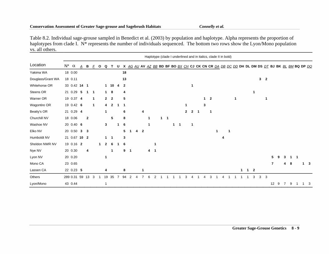
Conservation Assessment of Greater Sage-grouse and Sagebrush Habitats Connelly et al.
Greater Sage-Grouse Genetics 8 - 9
Table 8.2. Individual sage-grouse sampled in Benedict et al. (2003) by population and haplotype. Alpha represents the proportion of haplotypes from clade I. N* represents the number of individuals sequenced. The bottom two rows show the Lyon/Mono population vs. all others.
Haplotype (clade I underlined and in italics, clade II in bold)
Location N* α A B F O Q T U X AG AU AV AZ BB BD BF BO BX CH CJ CK CN CR DA DB DC DD DH DL DM DS DT BJ BK BL BM BQ DP DQ
Yakima WA 18 0.00 18
Douglass/Grant WA 18 0.11 13 3 2
Whitehorse OR 33 0.42 14 1 1 10 4 2 1
Steens OR 21 0.29 5 1 1 1 8 4 1
Warner OR 19 0.37 4 1 2 2 5 1 2 1 1
Wagontire OR 19 0.42 6 1 4 2 1 1 1 3
Beatty's OR 21 0.29 4 1 6 4 2 2 1 1
Churchill NV 18 0.06 2 5 8 1 1 1
Washoe NV 20 0.40 6 3 1 6 1 1 1 1
Elko NV 20 0.50 3 3 5 1 4 2 1 1
Humboldt NV 21 0.67 10 2 1 1 3 4
Sheldon NWR NV 19 0.16 2 1 2 6 1 6 1
Nye NV 20 0.30 4 1 9 1 4 1
Lyon NV 20 0.20 1 5 9 3 1 1
Mono CA 23 0.65 7 4 8 1 3
Lassen CA 22 0.23 5 4 8 1 1 1 2
Others 289 0.31 59 13 3 1 19 35 7 94 2 4 7 6 2 1 1 1 1 3 4 1 4 3 1 4 1 1 1 1 3 3 3
Lyon/Mono 43 0.44 1 12 9 7 9 1 1 3

Conservation Assessment of Greater Sage-grouse and Sagebrush Habitats Connelly et al.
Greater Sage-Grouse Genetics 8 - 10
Fig. 8.1. Phylogram (from Kahn et al. 1999) shows that the 21 mitochondrial DNA haplotypes are separated into two deep monophyletic clades. Bootstrap values greater than 50% are shown along the branches of the tree. Haplotypes from clade I and clade II are found in all greater sage-grouse populations sampled.

Conservation Assessment of Greater Sage-grouse and Sagebrush Habitats Connelly et al.
Greater Sage-Grouse Genetics 8 - 11
Fig. 8.2. From Oyler-McCance et al. (1999) (A) Neighbor-joining trees of microsatellite data using two different genetic distance measures. (B) Neighbor-joining tree of mitochondrial DNA genetic distances using allele frequencies and haplotype distances. Gunnison Sage-Grouse are identified with boxes.
Proportion ofshared alleles
Crawford
Gunnison Basin
Dove
Dry Creek
Cold Springs
Eagle
Blue Mountain
Middle Park
North Park
Chord distance
Gunnison Basin
Crawford
Dry Creek
Dove
Cold Springs
Eagle
Blue Mountain
North Park
Middle Park
A
Tamura
Crawford
Dry Creek
Dove Creek
Gunnison Basin
North Park
Cold Springs
Middle Park
Blue Mountain
Eagle
B

Conservation Assessment of Greater Sage-grouse and Sagebrush Habitats Connelly et al.
Greater Sage-Grouse Genetics 8 - 12
Fig. 8.3. Location of study populations from Benedict et al. (2003). The solid line denotes the delineation between the eastern and western subspecies of sage-grouse as proposed by Aldrich (1946).

Conservation Assessment of Greater Sage-grouse and Sagebrush Habitats Connelly et al.
Greater Sage-Grouse Genetics 8 - 13
Fig. 8.4. Phylogram of the strict-consensus tree of all sage-grouse haplotypes represented (from Benedict et al. 2003). Bootstrap values greater than 50% are shown along branches of the tree.

Conservation Assessment of Greater Sage-grouse and Sagebrush Habitats Connelly et al.
Greater Sage-Grouse Genetics 8 - 14
Fig. 8.5. Proportion of individual sage-grouse per population with novel haplotypes (from Benedict et al. 2003).
f
0%
10%
20%
30%
40%
50%
60%
70%
80%
90%
100%
Yakim
a (WA
)
Douglass/G
rant(W
A)
Whitehorse (O
R)
Steens (O
R)
Warner (O
R)
Wagontire (O
R)
Beatty's (O
R)
Churchill (N
V)
Washoe (N
V)
Elko (N
V)
Hum
boldt (NV
)
Sheldon (N
V)
Nye (N
V)
Lyon/Mono
Lassen (CA
)
Population
Per
cent
of I
ndiv
idua
ls w
ith N
ovel
Hap
loty
pes

Conservation Assessment of Greater Sage-grouse and Sagebrush Habitats Connelly et al.
Greater Sage-Grouse Genetics 8 - 15
Fig. 8.6. Neighbor-joining tree constructed using Wright’s (1978) modification of Roger’s genetic distance. Populations with boxes around them represent those populations that lie within the bounds of the Western sage-grouse. Populations without boxes lie within the bounds of Eastern sage-grouse.
Sheldon
Churchill
Nye
Douglass/Grant
Yakima
Mono
Lyon
Steens
Whitehorse
HumboldtWagontire
Warner
LassenWashoe
Beatty’s
Elko

Chapter 9
Effect of Harvest on Greater Sage-grouse

Effect of Harvest on Greater Sage-grouse 9 - 1
CHAPTER 9
Effect of Harvest on Greater Sage-grouse
Abstract. Harvest of greater sage-grouse (Centrocercus urophasianus) has occurred throughout recorded history, but relatively few studies address the impact of harvest on sage-grouse numbers. Harvest of greater sage-grouse occurs in 10 of the 11 western states in which they reside. Here we discuss current season structures and recent changes in sage-grouse hunting seasons. We also review the likely effects of hunting on sage-grouse populations based on published studies. Based on recent research, it appears that because greater sage-grouse experience low mortality over winter, mortality from hunter harvest in September and October may not be compensatory to a large extent. However, no studies have demonstrated that hunting is a primary cause of reduced numbers of greater sage-grouse.
Introduction
The impact of harvest on populations of many wildlife species remains uncertain
(Guttierrez 1994, Roy and Woolf 2001, Otis 2002, Williams et al. 2004). While there are numerous examples of sustainable harvest within high-quality habitats (Potts 1986, Hudson and Dobson 2001, Sutherland 2001, Willebrand and Hornell 2001, Gonzalez Voyer et al. 2003), excessive harvest can reduce spring breeding population size of gamebird species (Anderson and Burnham 1976, Small et al. 1991, Williams et al. 2004). Harvest of greater sage-grouse (Centrocercus urophasianus) has occurred throughout recorded history (Patterson 1952, Autenreith 1981), but relatively few studies address the impact of harvest on sage-grouse numbers. Given the declines in sage-grouse populations across the West (Connelly and Braun 1997), many hunters and biologists have expressed concern over the possible impacts of continued sport hunting of the species.
Harvest of greater sage-grouse occurs in 10 of the 11 western states in which they reside;
only Washington prohibits harvest. Neither Alberta nor Saskatchewan allows harvest. In the 1800s, heavy harvests decimated populations of greater sage-grouse, most states
then prohibited harvest and populations increased (Patterson 1952). Harvest regulations have fluctuated over the past 50 years as populations increased or declined (Autenreith 1981, Wambolt et al. 2002).
In 2003, opening dates for hunting greater sage-grouse ranged from 1 September to 11
October, but most states began their seasons in mid-September (Table 9.1). Season lengths ranged from 2 to 62 days with a mean length of 9 days. Only two states, Montana and Idaho, retain seasons of more than 9 days, while 5 of the 10 states have open seasons of 5 days or less. Recently, hunting seasons, and bag and possession limits, for greater sage-grouse have become more restrictive as states respond to declining populations (Table 9.1). For example, in the last 10 years, regulatory changes in 5 states reduced harvest opportunities. Wyoming shifted the opening date of the hunting season from early September to mid September in 1995 and changed the opening day to the last Saturday of September in 2002. Wyoming also shortened the season by 7 days, and reduced the bag and possession limits from 3 and 6 to 2 and 4, respectively. In

Conservation Assessment of Greater Sage-grouse and Sagebrush Habitats Connelly et al.
Effect of Harvest on Greater Sage-grouse 9 - 2
1999, Nevada closed hunting seasons in 6 counties and in 7 hunt units in two other counties; the state also shortened the season from 16 to 9 days in other areas. Nevada closed two more hunt units in 2001 and an additional unit in 2003. Utah changed the regulations for greater sage-grouse from a general hunt with 1 and 2 bird bag and possession limits, respectively, to permit-only hunts in 4 units. Total number of permits was 954 for a 9-day season with a 2-bird season limit. California reduced the number of permits by nearly half, from 325 to 175. South Dakota retained a 2-day season, but reduced the season limit from 2 birds to 1.
In contrast, Oregon increased hunter opportunity through increasing the number of
greater sage-grouse permits. In 2003, Oregon offered 1275 permits, 10 more than in 2001. This is less than a 1% increase in permit numbers. Regulations in Montana, Idaho, Nevada, Colorado, and North Dakota remained constant the past 3 years, but each state may have opened or closed specific hunting areas not reported here. For example, an area in Idaho closed to harvest since 1996 was opened in 2002.
Harvest
Currently available data indicate that the states of Montana, Idaho, Wyoming and Nevada, all with general greater sage-grouse hunting seasons, lead in estimated numbers of harvested greater sage-grouse (Table 9.2). Annual harvest estimates range from 12 in South Dakota to 7,576 in Idaho. Total annual harvest across the 10 states approximates 24,000 greater sage-grouse.
State wildlife management agencies reduce harvest opportunities to minimize the
possibilities that hunting may have a negative impact on populations of greater sage-grouse. Over the past 50 years, wildlife managers and scientists have recognized that sport hunting can reduce wildlife species (Bergerud 1985, Ellison 1991, Dixon et al. 1996, Williams et al. 2004) unless prevented through harvest regulations. For upland gamebird populations, harvest mortality that reduces the population for the subsequent spring breeding season is termed “additive” (Anderson and Burnham 1976, Williams et al. 2004). Each bird harvested is in addition to those killed naturally through disease, starvation, accidents or predation. Additive hunting mortality results in a spring breeding population lower than if harvest had not occurred. In contrast, mortality from hunters could reduce natural mortality through a number of density dependent mechanisms including reduced depredation or lower competition for food or shelter, such that total mortality is no higher than without harvest. This “compensatory” mortality does not reduce subsequent spring breeding population size below what it would have been due to natural mortality (Anderson and Burnham 1976). Partial compensation could also occur in hunted populations (Anderson and Burnham 1976). Robertson and Rosenberg (1988) also addressed the issue of compensatory and additive mortality and concluded that in natural populations hunting mortality usually falls between the 2 extremes of being totally additive or totally compensatory.
Life history characteristics of greater sage-grouse differ from many other upland game
birds. Many of these species have an r-selected strategy (Anderson 2002:54). They have high fecundity with large clutch sizes of 10-17 eggs, high annual rates of natural mortality, especially

Conservation Assessment of Greater Sage-grouse and Sagebrush Habitats Connelly et al.
Effect of Harvest on Greater Sage-grouse 9 - 3
over winter (40-70%), and short life spans of 1-2 years (Gullion 1984, Potts 1986, Petersen et al. 1988, Christensen 1996, Giudice and Ratti 2001). Removal of individuals through hunting likely compensates for the many birds that would die naturally during their first or second winter (Kokko 2001, Sutherland 2001). Greater sage-grouse, however, tend toward K-selected life history features, with relatively low productivity through clutch sizes of 6-9 eggs, low over-winter mortality rates of 2-20%, and long life spans of 3-6 years (Schroeder et al. 1999). “Hunting will not have as large an impact on a population exhibiting an r strategy as it will on one having a K strategy” (Anderson 2002:55). Although effects of hunting may be independent of life history features (r-K continuum) if post harvest survival or reproduction is largely density dependent, there is no published information suggesting that this is the case for sage-grouse. Moreover, Ellison (1991) concluded there is little evidence for density-dependent breeding in tetraonids and that hunting may result in an age structure that lowers a population’s productivity. Compensatory survival has been characterized as dogma within the field of wildlife management (Romesburg 1981, Warner 1992).
The appropriate harvest rate, expressed as percentage of the autumn population, remains
elusive for greater sage-grouse. Several studies have addressed this during recent decades. A harvest rate of 30% for greater sage-grouse in Idaho was deemed allowable in a non peer-reviewed report by Autenreith (1981), but he believed that this high rate was never reached in any area. In addition, he emphasized that in xeric areas close to urban centers, harvest should be more conservative than in more mesic areas. Forbs are readily available to grouse throughout mesic ranges and grouse do not congregate in restricted feeding areas in August and September as they do in xeric ranges with limited mesic sites. Autenreith (1981) argued that dispersed birds in more mesic ranges are not as vulnerable to harvest as aggregated birds in xeric ranges nearer urban centers.
Crawford (1982), Crawford and Lutz (1985), and Braun and Beck (1985) all examined
impacts of harvest through use of harvest figures, lek count trends, brood counts or with band recoveries. In Oregon, Crawford (1982:376) analyzed 20 years of data and reported that “the mortality from harvest may have been compensatory.” Crawford and Lutz (1985) concluded that while harvest may have short-term effects on greater sage-grouse populations through increased mortality, sport hunting was not responsible for the long-term decline in sage-grouse numbers in Oregon. Braun and Beck (1985) determined that 7 to 11% of the fall population was harvested in an area of Colorado and that harvest had no measurable effect on sage-grouse densities in the spring. They concluded that hunting mortality could remove 20 to 25% of the autumn population without being additive.
While greater sage-grouse populations declined further in the 1990s and states reduced
harvest opportunities, influence of harvest received little attention until late in the decade. Robert Gibson (personal communication) of the University of Nebraska examined population dynamics of 2 populations of greater sage-grouse in Mono County, California using data over a 45-year span. One population was isolated and the other was contiguous with populations in Nevada. Data used consisted of lek counts, numbers of birds shot per hunter in autumn, juveniles per hen in brood counts and in the fall bag, and number of birds inspected at check stations. He reported that the population contiguous with Nevada fluctuated independently of

Conservation Assessment of Greater Sage-grouse and Sagebrush Habitats Connelly et al.
Effect of Harvest on Greater Sage-grouse 9 - 4
hunting mortality. However, the isolated population fluctuated, in part, with number of birds examined at check stations the previous autumn. Gibson (1998) concluded in an unpublished abstract that hunting mortality could “depress and hold population levels of sage grouse well below carrying capacity” and that this “should be of widespread concern in the light of long term population declines and range fragmentation in this species.”1
Johnson and Braun (1999) used 23 years of hunter harvest and lek count data in a
population viability analysis (PVA) for greater sage-grouse in North Park, Colorado. A PVA can assess the risk of a species population going extinct based on its survival and production values (Boyce 1992). As a mortality factor for greater sage-grouse, Johnson and Braun (1999) reported that hunting mortality was compensatory up to a threshold level, and at or beyond that threshold, harvest may be additive. The level where harvest becomes additive was not reported.
In another 20-year study, Connelly et al. (2000a) monitored mortality of radio-marked
adult sage-grouse in Idaho. Adult females (n = 363) were affected by harvest more than adult males (n = 141). Autumn harvest caused 15% of known male mortality and 42% of known female mortality. Forty-six percent of all female mortality occurred during the hunting season (September and October) and harvest accounted for 91% of all female deaths. The sage-grouse hunting season in Idaho occurred in September and October. Post-hunting mortality (November-December) was only 1% for both genders combined (n = 103). Moreover, during the 4 post-hunting season months of November through February only 2% of the deaths of either sex occurred. The low over-winter mortality rate supports the contention that winter is not typically a difficult season for greater sage-grouse (Beck and Braun 1978, Remington and Braun 1988, Sherfy 1992).
Recognizing the typically low over-winter mortality of sage-grouse is vital to
understanding impacts of harvest. Robertson (1991) monitored radio-marked sage-grouse over 3 winters in southeastern Idaho. Sample sizes were small, 7, 7 and 9 birds, respectively, but only 1 death occurred over 3 winters, and the average survival over 3 winters was 96%. A recent analysis of 20 years of band-recovery data from North Park, Colorado provides more evidence that winter is not a period of great loss for sage-grouse.
Zablan et al. (2003) found no evidence that variation in winter precipitation affected annual survival rates of sage-grouse, further support for winter as a time of minimal mortality. In southwestern Idaho, Wik (2002) determined seasonal survival rates of radio-marked greater sage-grouse from spring 1999 through fall 2001. Six estimates of winter survival rates of various age and sex classes of grouse produced point estimates of 0.85, 0.87, 0.88, 0.90, 1.00, and 1.00, all exceeding the 0.80 minimum over-winter survival reported in the review by Schroeder et al. (1999).
1 Although we have generally avoided the use of personal communications and non peer-reviewed reports, there is a general lack of information on effects of hunting on sage-grouse. After careful consideration and discussions with the author and a California Department of Fish and Game biologist, we decided it was in the best interest of the resource to provide information from the Gibson report.

Conservation Assessment of Greater Sage-grouse and Sagebrush Habitats Connelly et al.
Effect of Harvest on Greater Sage-grouse 9 - 5
Because greater sage-grouse experience low mortality over winter, mortality from hunter harvest in September and October may not be compensatory to a large extent. What is the threshold point where harvest becomes additive? Based on a review of the literature, Connelly et al. (2000c) suggested that no more than 10% of the autumn population be removed through harvest. What are current harvest rates from autumn populations of greater sage-grouse? In Idaho, the harvest rate of adult females over 15 years averaged 6%, but in 6 of those years exceeded 10%, therefore Connelly et al. (2000a:230) concluded that for adult females “hunting losses are likely additive to winter mortality and may result in lower breeding populations.” More recently, Wik (2002) reported harvest rates in an area of southwestern Idaho to be 5% for males, 6% for adult females and 18% for sub-adult females, and suggested limiting harvest, especially of females. Zablan et al. (2003) considered recovery rates to reflect harvest rates since most recovered bands from greater sage-grouse were from hunter-killed birds. They reported that recovery rates varied from 14.0% to 18.7% in North Park, Colorado, but found no correlation between population fluctuations, as measured by lek counts and recovery data over the period of study. However, Zablan et al. (2003) suggested that lek counts were inadequate to index population changes or that sample sizes of banded birds were low. Wildlife management agencies have reduced hunting pressure and harvest rates through regulatory changes, but have not universally accepted a specific harvest rate. There may not be one harvest rate appropriate for all populations of greater sage-grouse. Zunino (1987) conducted a non-replicated experiment on 2 areas of Nevada to determine the response of sage-grouse density to harvest. Using autumn helicopter surveys that were assumed to count a constant proportion of the population, autumn sage-grouse densities were estimated in 1984 and 1985. Autumn sage-grouse populations on both the control (non-hunted) and treatment (hunted) areas increased between years. However, the increase in fall population density was 4 times greater on the control area than on the treatment area. These differences “were attributed to the treatments no harvest and harvest” (Zunino 1987:26).
Connelly et al. (2003) conducted the only other experimental study of greater sage-grouse
response to harvest. They used lek counts from 1996 to 2001 on 19 lek routes to assess response to 3 levels of harvest. All lek routes were in areas with the same harvest regulations in 1996 (30-day season, 3 bird bag, 6 in possession). In 1997 and continuing through 2001, regulations changed to either no hunting, a restrictive 7-day season with 1 bird bag, 2 in possession, or a moderate 23-day season with 2 bird bag, 4 in possession. Treatments (no hunting, restrictive, or moderate seasons) consisted of 5, 7 and 7 lek routes, respectively. Lek routes were also categorized as being in lowland areas close (< 1.5 hours drive) to major cities and towns or in high elevation mountain valleys farther from urban centers. After reducing harvest opportunities, areas that remained open to hunting had lower rates of increase than did areas with no hunting (Connelly et al. 2003). Both the moderate and restrictive hunting seasons produced harvests that apparently slowed population recovery (Connelly et al. 2003). Populations in low elevation habitats, close to urban centers and isolated because of habitat fragmentation, may be less able to withstand a harvest rate that has little or no effect on populations in more extensive, contiguous, remote, or mesic areas (Gibson 1998, Connelly et al. 2003).

Conservation Assessment of Greater Sage-grouse and Sagebrush Habitats Connelly et al.
Effect of Harvest on Greater Sage-grouse 9 - 6
Regulations for harvest of greater sage-grouse should minimize the possibility of negative effects. Therefore, units with dissimilar vegetative, physical or ecological attributes may differ in appropriate hunting season length and bag limits. However, several investigators have suggested that hunting seasons should be established with low rates of harvest (Schroeder et al. 1999, Connelly et al. 2000c, Wambolt et al. 2002), which should allow populations to increase if habitat quality is not limiting population numbers (Connelly et al. 2003). States do not presently determine autumn population sizes of greater sage-grouse.
No studies have demonstrated that hunting is a primary cause of reduced numbers of greater sage-grouse. Many studies support habitat-based reasons for sage-grouse declines (Swenson et al. 1987, Connelly and Braun 1997, Connelly et al. 2000b, Leonard et al. 2000, Aldridge and Brigham 2002, Pedersen et al. 2003). While eliminating harvest as a source of mortality did not produce any increase in greater sage-grouse numbers in Washington, likely because of habitat issues (Schroeder et al. 2000), reducing harvest may aid in population recovery in specific cases (Connelly et al. 2003).
Harvest of greater sage-grouse provides population data not easily obtained except through costly radio-telemetry studies of specific populations. Wings from hunter-harvested birds allow determination of sex and age ratios, average production per hen, and percentage of successful hens (see Chapter 6 for additional information). In conjunction with population trend counts, these data contribute to understanding the dynamics of sage-grouse in each management unit.
An appropriate harvest rate has not been determined for greater sage-grouse populations. Harvest equal to 5-10% of the autumn population may be appropriate, but assumes detailed and specific knowledge of population size in September or October. Given the uncertainty in abundance estimates for breeding season populations, expecting any state to adequately determine size of any population of greater sage-grouse in fall may not be realistic.
Literature Cited
Aldridge, C. L., and R. M. Brigham. 2002. Sage-grouse nesting and brood habitat use in southern Canada. Journal of Wildlife Management 66:433-444.
Anderson, D. R., and K. P. Burnham. 1976. Population ecology of the mallard: VI. The effect of exploitation on survival. U.S. Fish and Wildlife Service, Resource Publication 128, Washington, D.C.
Anderson, S. H. 2002. Managing our wildlife resources. Fourth edition. Prentice Hall, Upper Saddle River, New Jersey, USA.
Autenrieth, R. E. 1981. Sage grouse management in Idaho. Idaho Department of Fish and Game Wildlife Bulletin 9. Boise, Idaho.
Beck, T. D. I., and C. E. Braun. 1978. Weights of Colorado sage grouse. Condor 80:241-243.
Bergerud, A. T. 1985. The additive effect of hunting mortality on the natural mortality rates of grouse. Pages 345-366 in S. L. Beasom and S. F. Roberson, editors. Game harvest management. Caesar Kleberg Wildlife Research Institute,

Conservation Assessment of Greater Sage-grouse and Sagebrush Habitats Connelly et al.
Effect of Harvest on Greater Sage-grouse 9 - 7
Kingsville, Texas. Boyce, M. S. 1992. Population viability analysis. Annual Review of Ecology and
Systematics 23:481-506. Braun, C. E., and T. D. I. Beck. 1985. Effects of changes in hunting regulations on sage
grouse harvest and populations. Pages 335-343 in S. L. Beasom and S.F. Roberson, editors. Game harvest management. Caesar Kleberg Wildlife Research Institute, Kingsville, Texas.
Christensen, G. C. 1996. Chukar (Alectoris chukar). in The Birds of North America, No. 258. A. Poole, and F. Gill, editors. The Birds of North America, Inc., Philadelphia, Pennsylvania.
Connelly, J. W., and C. E. Braun. 1997. Long-term changes in sage grouse Centrocercus urophasianus populations in western North America. Wildlife Biology 3:229-234.
Connelly, J. W., A. D. Apa, R. B. Smith, and K. P. Reese. 2000a. Effects of predation and hunting on adult sage-grouse Centrocercus urophasianus in Idaho. Wildlife Biology 6:227-232.
Connelly, J. W., K. P. Reese, R. A. Fischer, and W. L. Wakkinen. 2000b. Response of a sage grouse breeding population to fire in southeastern Idaho. Wildlife Society Bulletin 28:90-96.
Connelly, J. W., M. A. Schroeder, A. R. Sands, and C. E. Braun. 2000c. Guidelines to manage sage grouse populations and their habitats. Wildlife Society Bulletin 28:967-985.
Connelly, J. W., K. P. Reese, E. O. Garton, and M. L. Commons-Kemner. 2003. Response of greater sage-grouse Centrocercus urophasianus populations to different levels of exploitation in Idaho, USA. Wildlife Biology 9:335-340.
Crawford, J. A. 1982. Factors affecting sage grouse harvest in Oregon. Wildlife Society Bulletin 10:374-377.
Crawford, J. A., and R. S. Lutz. 1985. Sage grouse population trends in Oregon, 1941- 1983. Murrelet 66:69-74.
Dixon, K. R., M. A. Horner, S. R. Anderson, W. D. Henriques, D. Durham, and R. J. Kendall. 1996. Northern bobwhite habitat use and survival on a South Carolina plantation during winter. Wildlife Society Bulletin 24:627-635.
Ellison, L. N. 1991. Shooting and compensatory mortality in tetraonids. Ornis Scandinavica 22:229-240.
Gibson, R. 1998. Effects of hunting on the population dynamics of two sage grouse populations in Mono County, California. Western Sage and Columbian Sharp- tailed Grouse Workshop 21:15.
Giudice, J. H., and J. T. Ratti. 2001. Ring-necked pheasant (Phasianus colchicus). in The Birds of North America, No. 572. A. Poole, and F. Gill, editors. The Birds of North America, Inc., Philadelphia, Pennsylvania.
Gonzalez Voyer, A., K. G. Smith, and M. Festa-Bianchet. 2003. Dynamics of hunted and unhunted mountain goats Oreamnos americanus populations. Wildlife Biology 9:213-218.
Gullion, G. W. 1984. Ruffed grouse management – where do we stand in the eighties? Pages 169-181 in W. L. Robinson, editor. Ruffed grouse management: state of
Conservation Assessment of Greater Sage-grouse and Sagebrush Habitats Connelly et al.
Effect of Harvest on Greater Sage-grouse 9 - 8
the art in the early 1980’s. North Central Section of The Wildlife Society, BookCrafters, Chelsea, Michigan.
Guttierrez, R. J. 1994. North American upland gamebird management at crossroads: which road will we take? North American Wildlife and Natural Resources Conference 59:494-497.
Hudson, P. J., and A. P. Dobson. 2001. Harvesting unstable populations: red grouse Lagopus lagopus scoticus in the United Kingdom. Wildlife Biology 7:189-195.
Johnson, K. H., and C. E. Braun. 1999. Viability and conservation of an exploited sage grouse population. Conservation Biology 13:77-84.
Kokko, H. 2001. Optimal and suboptimal use of compensatory responses to harvesting: timing of hunting as an example. Wildl. Biol. 7:141-150.
Leonard, K. M., K. P. Reese, and J. W. Connelly. 2000. Distribution, movements and habitats of sage grouse Centrocercus urophasianus on the Upper Snake River Plain of Idaho: changes from the 1950s to the 1990s. Wildlife Biology 6:265- 270.
Otis, D. L. 2002. Survival models for harvest management of mourning dove populations. Journal of Wildlife Management 66:1052-1063.
Patterson, R. L. 1952. The sage grouse in Wyoming. Sage Books, Inc., Denver, Colorado.
Pedersen, E. K., J. W. Connelly, J. R. Hendrickson, and W. E. Grant. 2003. Effect of sheep grazing and fire on sage grouse populations in southeastern Idaho. Ecological Modeling 165:23-47.
Petersen, L. R., R. T. Dumke, and J. M. Gates. 1988. Pheasant survival and the role of predation. Pages 165-196 in D. L. Hallett, W. R. Edwards, and G. V. Burger, editors. Pheasants: symptoms of wildlife problems on agricultural lands. North Central section of The Wildlife Society, Bloomington, Indiana.
Potts, G. R. 1986. The partridge: pesticides, predation, and conservation. Collins, London.
Remington, T. E., and C. E. Braun. 1988. Carcass composition and energy reserves of Sage grouse during winter. Condor 90:15-19. Park, Colorado. Journal of Wildlife Management 49:1055-1061.
Robertson, M. D. 1991. Winter ecology of migratory sage grouse and associated effects of prescribed fire in southeastern Idaho. M.S. Thesis, University of Idaho, Moscow, Idaho.
Robertson, P. A., and A. A. Rosenberg. 1988. Harvesting gamebirds. Pages 177-201 in P. J. Hudson and M. R. W. Rands, editors. Ecology and Management of Gamebirds. BSP Professional Books, Oxford, United Kingdom. Romesburg, H. C. 1981. Wildlife science: gaining reliable knowledge. Journal of Wildlife Management 45:293-313. Roy, C., and A. Woolf. 2001. Effects of hunting and hunting-hour extension on
mourning dove foraging and physiology. Journal of Wildlife Management 65:808-815.
Schroeder, M. A., J. R. Young, and C. E. Braun. 1999. Sage grouse (Centrocercus urophasianus). in The Birds of North America, No. 425. A. Poole and F. Gill, editors. The Birds of North America, Inc., Philadelphia, Pennsylvania.

Conservation Assessment of Greater Sage-grouse and Sagebrush Habitats Connelly et al.
Effect of Harvest on Greater Sage-grouse 9 - 9
Schroeder, M. A., D. W. Hays, M. F. Livingston, L. E. Stream, J. E. Jacobson, and D. J. Pierce. 2000. Changes in the distribution and abundance of sage grouse in Washington. Northwestern Naturalist 81:104-112.
Sherfy, M. H. 1992. The influence of season, temperature, and wind speed on sage grouse metabolism. M.S. Thesis, University of New Hampshire, Durham, New Hampshire.
Small, R. J., J. C. Holzwart, C. James, and D. H. Rusch. 1991. Predation and hunting mortality of ruffed grouse in central Wisconsin. Journal of Wildlife Management 55:512-520.
Sutherland, W. J. 2001. Sustainable exploitation: a review of principles and methods. Wildlife Biology 7:131-140.
Swenson, J. E., C. A. Simmons, and C. D. Eustace. 1987. Decrease of sage grouse Centrocercus urophasianus after ploughing of sagebrush steppe. Biological Conservation 41:125-132.
Wambolt, C. L., A. J. Harp, B. L. Welch, N. Shaw, J. W. Connelly, K. P. Reese, C. E. Braun, D. A. Klebenow, E. D. McArthur, J. G. Thompson, L. A. Torell, and J. A. Tanaka. 2002. Conservation of greater sage-grouse on public lands in the western U.S.: implications of recovery and management policies. Policy Analysis Center for Western Public Lands, Policy Paper SG-02-02. Caldwell, Idaho.
Warner, R. E. 1992. Long-term perspectives of upland game bird research in North America. Pages 709-717 in D. R. McCullough and R. H. Barrett, editors.
Wildlife 2001: populations. Elsevier Science Publishers, Ltd., Sessex, United Kingdom. Wik, P. 2002. Ecology of greater sage-grouse in south-central Owyhee County, Idaho.
M.S. Thesis, University of Idaho, Moscow, Idaho. Willebrand, T., and M. Hornell. 2001. Understanding the effects of harvesting willow
ptarmigan Lagopus lagopus in Sweden. Wildlife Biology 7:205-212. Williams, C. K., R. S. Lutz, and R. D. Applegate. 2004. Winter survival and additive
harvest in northern bobwhite coveys in Kansas. Journal of Wildlife Management 68:94-100.
Zablan, M. A., C. E. Braun, and G. C. White. 2003. Estimation of greater sage-grouse survival in North Park, Colorado. Journal of Wildlife Management 67:144-154.
Zunino, G. W. 1987. Harvest effects on sage grouse densities in northwest Nevada. M.S. Thesis, University of Nevada, Reno, Nevada.

Conservation Assessment of Greater Sage-grouse and Sagebrush Habitats Connelly et al.
Effect of Harvest on Greater Sage-grouse 9 - 10
Table 9.1. Calendar year 2003 hunting seasons for greater sage-grouse. Opening date Number State for state or area of days Bag and possession limit Montana 1 September 62 3/6 Idaho (1) 20 September 23 2/4 (2) 20 September 7 1/2 Wyoming 27 September 9 2/4 Nevada (1) 11 October 9 2/4 (2) 20 September 2 3/6 with 75 permits (3) 27 September 2 3/6 with 75 permits (4) 27 September 2 3/6 with 75 permits Utah (1) 20 September 9 2/2 season limit, 431 permits (2) 20 September 9 2/2 season limit, 211 permits (3) 20 September 9 2/2 season limit, 200 permits (4) 20 September 9 2/2 season limit, 112 permits Colorado 13 September 7 2/4 Oregon 6 September 5 2/2 season limit, 12 areas
with 10 to 225 permits, total of 1,275 permits
California (1) 13 September 2 2/2 season limit, 100 permits (2) 13 September 2 2/2 season limit, 40 permits (3) 13 September 2 1/1 season limit, 25 permits (4) 13 September 2 1/1 season limit, 10 permits South Dakota 24 September 2 1/1 season limit North Dakota 15 September 3 1/1

Conservation Assessment of Greater Sage-grouse and Sagebrush Habitats Connelly et al.
Effect of Harvest on Greater Sage-grouse 9 - 11
Table 9.2. Annual statewide harvest estimates for greater sage-grouse. State Year1 Harvest Montana 2002 5,475 Idaho 2002 7,576 Wyoming 2002 4,835 Nevada 2002 3,940 Utah 2003 1,049 Colorado 2002 307 Oregon 2003 979 California 2003 170 South Dakota 2003 12 North Dakota 2002 45
1 Most recent data available.

Chapter 10
Predation, Parasites and Parasites

Predation, Parasites and Pathogens 10 - 1
CHAPTER 10
Predation, Parasites and Pathogens
Abstract. In this chapter we discuss the diversity of predators, parasites and diseases-causingpathogens that influence greater sage-grouse (Centrocercus urophasianus) the species range. Despitethe prevalence of organisms that effect individual birds, population-level effects have been rarelydocumented. Concerns about predation have generally been indirectly addressed with habitatmanagement. The newest observed disease, West Nile virus, has shown greater virulence than anyinfection or infestation noted so far.
Predation
As with most species of game birds, sage-grouse have many predators. Throughout mostof the species’ range, coyotes (Canis latrans), badgers, (Taxidea taxus), bobcats (Felis rufus) andseveral species of raptors are common predators of juvenile and adult sage-grouse (Patterson 1952,Schroeder et al. 1999, Schroeder and Baydack 2001). Additionally, coyotes, badgers, groundsquirrels (Spermophillus spp.), common ravens (Corvus corax), and magpies (Pica pica) commonlyprey on sage-grouse eggs (Patterson 1952, Schroeder et al. 1999, Schroeder and Baydack 2001).Many additional predators can kill and consume younger birds including the common raven,northern harrier (Circus cyaneus), and weasel (Mustella spp.) (Schroeder et al. 1999). Theabundance of red fox (Vulpes vulpes) and raccoon (Procyon lotor) may have substantially increasedin sage-grouse habitats because of landscape changes (Fichter and Williams 1967, Bunnell 2000,Connelly et al. 2000a).
Although there is little published information supporting the notion that predation is a majorlimiting factor on sage-grouse Connelly and Braun 1997, Connelly et al. 2000b, Schroeder andBaydack 2001), arguments continue to be made supporting predator control as an importantmanagement action (Wambolt et al. 2002). Two non peer-reviewed studies (Batterson and Morse1948, Autenrieth 1981) suggested that nest predation due to corvids may limit sage-grouse numbers.More recently, numerous investigators have documented sage-grouse survival and nest success(Gregg 1991, Robertson 1991, Connelly et al. 1993, Gregg et al. 1994, Holloran 1999, Lyon 2000,Wik 2002). Only two of these studies (Gregg 1991, Gregg et al. 1994) indicated that predation waslimiting sage-grouse populations by decreasing nest success, but both of these indicated that lownest success due to predation was ultimately related to poor nesting habitat. Most reported nestsuccess rates are >40% (see chapter 3), suggesting that nest predation is not a widespread problem.Additionally, relatively high survival of adult birds (Zablan et al. (2003) and recent resultsdemonstrating that coyote control in an area of Wyoming failed to produce an effect on nestingsuccess (Slater 2003), further reinforce the idea that predation is not a widespread factor acting todepress sage-grouse populations. Thus, rigorous field studies using radio telemetry have generallyfailed to support these early findings.
In order to understand the possible impacts of predators on sage-grouse, it is important tounderstand the dynamics and behavior of predator populations. There are no predators within therange of sage-grouse that depend on sage-grouse as their primary food source; many depend

Conservation Assessment of Greater Sage-grouse and Sagebrush Habitats Connelly et al.
Predation, Parasites and Pathogens 10 - 2
primarily on rodents and lagomorphs and feed on sage-grouse opportunistically (see Bump et al.1947, Angelstam 1986, Marcström et al. 1988, and Myrberget 1988 for examples). Consequently,the dynamics of a predator population and its primary food source can have observable impacts ona grouse population (Schroeder and Baydack 2001). When the primary food source is relativelyrare, then a predator may spend more time searching for food, and consequently may be more likelyto encounter a grouse or its nest (Angelstam 1983).
Predation may influence the population dynamics of grouse by reducing nest success,survival of juveniles (especially during the first few weeks after hatch), and annual survival ofbreeding-aged birds. The low survival of sage-grouse in the Strawberry Valley of Utah has beenattributed to an unusually high density of red foxes (Bunnell 2000). Nest success is extremelyvariable and differences in success have been attributed to variation in habitat and managementstrategy (Connelly et al. 1991, Gregg et al. 1994, Connelly et al. 2000b). Although sage-grouse maypartly compensate for predation pressure on nests by renesting (Schroeder 1997), habitat insufficient quality and quantity often has been stated as an important goal for reducing the effects ofpredation (Connelly et al. 1991, 2000b). Survival of juveniles is clearly low, but is also difficult toaccurately assess (Crawford et al. 2004). Unlike nesting habitat, management of brood-rearinghabitat has focused on increasing the density and diversity of forbs (Klott and Lindzey 1990, Pyleand Crawford 1996, Sveum et al. 1998b), rather than improving vegetation to reduce predation(Edelmann et al. 1998). Although there have been many observations and recommendationsconcerning the importance of suitable habitat for reducing predation pressure on adults, detailedstatistics have been difficult to obtain (Schroeder and Baydack 2001).
The quantity, quality, and configuration of habitat clearly has the potential to impact predatorbehavior and dynamics (Chapters 4, 12). These considerations include, but are not limited to, escapecover at nests (Connelly et al. 1991, Gregg et al. 1994) and visibility at leks (Hartzler 1974). Inaddition, several investigators have suggested that adequate feeding areas may minimize risksassociated with increased travel and time spent in riskier habitats (Gregg et al. 1993, Fischer et al.1996, Pyle and Crawford 1996).
Landscape fragmentation, agricultural habitats, and human populations have the potentialto increase predator populations, and hence, predation pressure on grouse populations, as shown forcorvids, domestic cats, and dogs (see Chapter 12). This potential for increased predation pressurein fragmented habitats is similar to what has been observed for grouse in Europe, where the patternis well documented (Andrén et al. 1985, Andrén and Angelstam 1988, Bernard-Laurent and Magnani1994, Kurki et al. 1997).
Although predator controls have been tried within the range of sage-grouse (Batterson andMorse [1948] removed many common ravens on an area in Oregon and there was a short-termincrease in nest success), the cost effectiveness and long-term impacts of the removal on thebehavior, genetics, and abundance of sage-grouse have not been examined (Schroeder and Baydack2001). There also has been a more recent recognition of the broader financial and political cost to

Conservation Assessment of Greater Sage-grouse and Sagebrush Habitats Connelly et al.
Predation, Parasites and Pathogens 10 - 3
removing predators (Messmer et al. 1999). Because of these considerations, predator managementfor sage-grouse has generally been addressed with the "manipulation of habitat, because it isbelieved to be the most economical, efficient, and viable long-term strategy to enhance populations"(Schroeder and Baydack 2001:28).
Parasites and Pathogens
Introduction
Greater sage-grouse host a variety of potentially pathogenic organisms. However, the merepresence of such organisms does not necessarily indicate a population level effect. During the1940's and 50's there was widespread belief, among both managers and laypersons, that diseaseswere responsible for heavy annual losses of gamebirds, including greater sage-grouse (Patterson1952, Herman 1963). To the average person, the presence of parasites and disease producingorganisms was synonymous with "disease" itself. Herman (1963) also reported that his review ofthe pertinent literature uncovered frequent references to 'the' greater sage-grouse disease, as thoughthe authors were convinced that one specific agent could be the "universal root of all losses". Inreality, some background level of parasites and disease producing organisms is normal and does nottypically cause any significant alteration in structure or function of the population of the host species(Patterson 1952, Herman 1963). However, under certain circumstances a disease-causing agent mayincrease to a level that local populations are impacted (Herman 1963). Such circumstances mayinclude extremes in precipitation, poor nutrition or the introduction of an exotic disease agent.
The parasites and diseases affecting greater sage-grouse have conformed to this pattern.Most of these parasites and diseases (Table 10.1) have not resulted in widespread population levelimpacts to greater sage-grouse. Those outbreaks of disease that have resulted in noteworthymorbidity and mortality were typically discovered under conditions of high numbers of grouse beingconcentrated due to dry conditions when water was scarce and large numbers of grouse likelycontaminated water and soil with fecal material. Even in these cases there was insufficient evidenceto conclude that disease was responsible for major declines across any extensive area of the birds'range (Patterson 1952).
Even so, there have been few systematic surveys for parasites or infectious diseasescompleted in greater sage-grouse, especially in recent years. This problem has been exacerbated bythe ineffectiveness of some techniques for detecting pathogens that are present, or forinappropriately labeling a pathogen as present when it is absent. Therefore, the role diseases andparasites play in population declines across their range is essentially unknown. This fact, coupledwith the emergence of new infectious diseases and the increasing numbers of small, isolatedpopulations of greater sage-grouse that may be more vulnerable to population level effects, suggeststhis field deserves further study.

Conservation Assessment of Greater Sage-grouse and Sagebrush Habitats Connelly et al.
Predation, Parasites and Pathogens 10 - 4
Of current concern is the emergence of the West Nile virus (WNV). This disease was exoticto the United States but is now considered endemic. It was first documented on the east coast in1999 and has advanced rapidly across the nation. Greater sage-grouse were first documented to havecontracted and succumbed to WNV in northeast Wyoming, eastern Montana and southeast Albertain the summer of 2003, although one Wyoming bird actually died in 2002 but was not diagnoseduntil 2003 (D.E. Naugle, Personal Communication).
The following describes known parasites and diseases of greater sage-grouse and theirimplications to the bird. Many sources of information have not been published in the scientificliterature, but instead appear in agency reports and proceedings. Where necessary we have includedthe references to provide a more through understanding of parasites and diseases in greatersage-grouse.
Macro-Parasites
Endoparasites. Protozoa. Coccidiosis. Coccidiosis in greater sage-grouse is the diseasecaused by the effect of one or more species of the protozoan genus Eimeria (Jolley 1982). Threespecies of the genus are known in greater sage-grouse: E. angusta, E. centrocerci, and E. pattersoni.E. angusta has been the most frequently documented species associated with coccidiosis (Thorne1969). Diarrhea, which is characteristic of the disease, is caused when the parasites develop in anddamage the mucosal lining of portions of the digestive tract. Transmission occurs when susceptiblebirds ingest feed or water contaminated by sporulated oocysts from feces of infected birds (Jolley1982). When large numbers of oocysts are found in the feces of live birds concurrent with diarrheaand emaciation, coccidiosis should be suspected as the cause of illness (Friend and Franson 1999).However, a diagnosis as a cause of death requires a necropsy as well. Diarrhea is caused by anumber of pathogens and oocysts observed in feces may or may not be those of the pathogenicspecies.
Historically, coccidiosis was the most important known parasitic disease of greatersage-grouse and has been, to date, the most prevalent of all known diseases affecting greatersage-grouse. In some site-specific locations, significant losses of young greater sage-grouse weredocumented in Wyoming, Colorado and Idaho from 1932-1953 (Honess and Post 1968). Most casesof coccidiosis in greater sage-grouse were discovered in areas where large numbers of birds werecongregated resulting in fecal contamination of soil and water.
Greater sage-grouse mortalities attributed to coccidiosis have not been documented since theearly 1960s. This may be the result of decreased greater sage-grouse densities. Investigatorsestimated 2,000 greater sage-grouse occupied a 2.59 km2 (1 mi2) alfalfa field prior to a coccidiosisoutbreak in 1932 (Honess and Post 1968). There are no reports of similar densities being observedin more recent history. Any attempt to hold captive greater sage-grouse (or other game birds) shouldinclude a plan to prevent coccidiosis before clinical signs appear (Jolley 1982).

Conservation Assessment of Greater Sage-grouse and Sagebrush Habitats Connelly et al.
Predation, Parasites and Pathogens 10 - 5
Hemosporidiosis (avian malaria). Hemosporidia are microscopic, intracellular parasiticprotozoans found within the blood cells and tissues of avian hosts (Atkinson 1999). Three closelyrelated genera, Plasmodium, Haemoproteus and Leucocytozoon are commonly found in wild birds(Atkinson 1999), including greater sage-grouse (Stabler et al. 1977, Gibson 1990, Boyce 1990,Deibert and Boyce 1997, Johnson and Boyce 1991, Dunbar et al. 2003). Hemosporidia aretransmitted from bird to bird by a variety of insects including mosquitoes, black flies and bitingmidges (Atkinson 1999). A distantly related flagellate parasite, Trypanosoma avium, has beendocumented in greater sage-grouse (Stabler et al. 1977) but neither clinical signs nor implicationsto individual hosts or populations have been described.
In highly susceptible bird species and age classes, infections may result in death (Atkinson1999). In greater sage-grouse, significant mortalities have not been well documented and most ofthe research conducted has centered around the effect of blood parasites (Plasmodium,Haemoproteus) on mate selection and breeding success. The traditional view that blood parasitesare only slightly or not pathogenic has been challenged with recent research (Bennett et al. 1993,Nordling et al. 1998, Raidal and Jaensch 2000). The need for control of hemosporidiosis in greatersage-grouse populations has not been indicated. Such control would require control of insect vectorsrather than treatment or prevention in birds themselves.
Sarcocystis. Salt (1958) described Sarcocystis releyi in greater sage-grouse however Jolley(1982) maintained that reports of S. releyi in gallinaceous and other birds were probably incorrectand involved other species of Sarcocystis. Regardless, there is no evidence to suggest significantimplications or the need for control in greater sage-grouse. Sarcocysts are ubiquitous in wild speciesand generally cause little or no pathology.
Trichomoniasis. Although large numbers of Tritrichomonas simoni were found in all healthygreater sage-grouse examined (Honess 1955), the parasite is not known to be pathogenic (Jolley1982).
Platyhelminthes. Tapeworms. Greater sage-grouse are the only known host of the cestodetapeworm Raillietina centrocerci (Honess 1982a). Raillietina cesticillus and Rhabdometranullicollis have also been reported (Keller et al. 1941, Simon, 1940). Leidy (1887) reported thecestode Hymenolepis microps, however Simon (1940) believed this to be a mistaken identification.Greater sage-grouse show no apparent clinical signs of parasitism even though the tapeworms maydistend the intestine and even dangle from the vent (Honess 1982a). Even the most heavilyparasitized birds will be in good physical condition (Thorne 1969). Although Kerwin (1971, citedin the Canadian Sage Grouse Recovery Strategy) felt the role of R. centrocerci was overlooked asa mortality factor, Honess (1982a) suggested the relationship was an almost perfect adjustmentbetween the host and its parasite. While unsightly, these tapeworms cannot parasitize humans anddo not affect the quality of greater sage-grouse meat.

Conservation Assessment of Greater Sage-grouse and Sagebrush Habitats Connelly et al.
Predation, Parasites and Pathogens 10 - 6
Nematoda. Gizzard worms. Gizzard worms belong to the genera Habronema and Acuaria(Cheilospirura). While Bergstrom (1982) indicated severe infestations of A. centrocerci couldthreaten greater sage-grouse in local areas, gizzard worms have only been seen occasionally and thusare not thought to present an important threat.
Cecal worms. Cecal worms of the genus Heterakis have been reported in greater sage-grouse(Simon 1940, Honess and Winter 1956). H. gallinarum is an important avian parasite because itseggs carry Histomonas meleagridis, the protozoan that causes the disease, avian blackhead. Thisdisease is important in domestic fowl and game bird farms (Bergstrom 1982). Because developmentof H. gallinarum can be influenced by temperature fluctuations, fluctuations in parasite abundancecould be linked with weather conditions (Saunders et al. 2002). The documentation of cecal wormsin greater sage-grouse suggests the possibility of exposure to H. meleagridis, however thedocumentation cited by Simon (1940) consisted solely of a personal communication with aninvestigator that identified H. gallinae in a single greater sage-grouse specimen. Since blackheaddisease has never been diagnosed in greater sage-grouse (free-ranging or captive), neither the diseasenor its parasite vector is considered a threat to greater sage-grouse. Cecal worms (Trichostrongylustenuis) in red grouse (Lagopus lagopus scoticus) have been linked with the population fluctuationsor cycles (Hudson et al. 1998).
Filarid worms. A filarial nemotode, Ornithofilaria tuvensis, has been identified in greatersage-grouse but its presence is rare (Hepworth 1962). These white, hairlike worms were found inthe connective tissue between the skin and breast muscles. Some birds observed where the knowninfected specimens were taken appeared unable to fly. However none of these birds were collectedfor analysis.
Ectoparasites. Mallophaga (lice). Three species of chewing (bird) lice have been identifiedon greater sage-grouse: Gonoides centrocerci, Lagopoecus gibsoni and L. perplexus. Chewing liceare small, wingless and dorso-ventrally flattened insects that feed on fragments of skin and feathers.Heavy infestations may cause irritation to the host but there are no known serious implications forwildlife (Honess 1982b). Studies have been made regarding the presence and prevalence of lice andother parasites as it relates to mate selection and breeding success by birds, including greatersage-grouse (Boyce 1990, Deibert 1995). These relationships may be important to the long-termecology and co-evolution of greater sage-grouse and the parasites; however, they have not beenshown to be significant to the immediate status of greater sage-grouse populations.
Acarina (ticks). Two species of hard tick have been identified on greater sage-grouse:Haemaphysalis chordeilis and Haemaphysalis leporis-palustris. Early authors described the speciesHaemaphysalis cinnabarina (Parker et al. 1932, Simon 1940); however, Kingston and Honess(1982) report that H. cinnabarina does not occur in North America, and all references to this speciesshould be referred to H. chordeilis. Ticks have been implicated in one greater sage-grouse mortalityevent that is discussed under the bacterial disease tularemia. Ticks can also cause "tick paralysis"in some hosts which is caused by a neurotoxin released by feeding adult female ticks (Honess and

Conservation Assessment of Greater Sage-grouse and Sagebrush Habitats Connelly et al.
Predation, Parasites and Pathogens 10 - 7
Bergstrom 1982). Ticks are not considered a threat to greater sage-grouse populations because theyare so infrequently observed on greater sage-grouse. Given the number of greater sage-grousehandled by researchers and hunters each year, and the relative ease in which ticks can be observed,more ticks would be reported if their presence was significant.
Diptera (flies, mosquitoes, midges, keds). Many diptera are pests and cause distress to thehosts on which they feed. Some diptera are important vectors of animal diseases, some of which willbe discussed below e.g. West Nile virus. High numbers of keds were detected on about 25% ofapproximately 200 greater sage-grouse captured in the Montana Mountains of northern Nevada in2002 (M.R. Dunbar, personal communication). These keds were identified as Ornithomyiaanchineuria. Keds have not been documented on greater sage-grouse elsewhere.
Pathogens
Bacteria. Salmonellosis. Bacteria of the genus Salmonella are responsible for severaldiseases of birds such as pullorum and fowl typhoid (Thorne 1969). However, the only instance inwhich a Salmonella sp. has been documented as a disease agent in greater sage-grouse was aWyoming case of dysentery characterized by debilitation and occasional death caused by stagnantand contaminated water supplies (Post 1960). This was probably a different species of Salmonellathan those that cause pullorum and typhoid (W. Cook, personal communication). Studies havedisclosed a much lower infection rate in wild birds than those in captivity and have causedinvestigators to conclude that, in general, salmonellosis is not an important disease of free-rangingwild birds (Friend 1999a).
Tularemia. Tularemia is primarily a tick-borne disease of mammals, but natural infectionsby Francisella tularensis have caused die-offs of ruffed grouse (Bonasa umbellus) and other grousespecies (Friend 1999b). Parker et al. (1932) studied an epizootic in greater sage-grouse in Montana.These grouse were heavily infested with a bird tick, Haemaphysalis chordeilis and infected withFrancisella tularensis. Hopla (1974) concluded that it was likely the tularemia, the tick, or both weremajor factors in the mortalities of these grouse. There have been no other reports of tularemia ingreater sage-grouse and it is not currently a disease of concern because of the lack of tickinfestations as noted above in the tick section.
Colibacillosis. Honess and Post (1968) reported that captured sick greater sage-grouseassociated with an outbreak of coccidiosis were also bacteremic with Escherichia coli. E. coli hasmany strains that vary in virulence and pathogenicity (Thorne 1982). It is found in the lowerintestine and is frequently a secondary invader that complicates primary infections. Diarrhea isclinical indicator of a possible pathogenic infection. While the presence of E. coli is probablyunder-reported, it is not believed to be a threat to wild populations of greater sage-grouse becauseit has only been shown to cause acute mortality in captive birds kept in unsanitary conditions (Friend1999b).

Conservation Assessment of Greater Sage-grouse and Sagebrush Habitats Connelly et al.
Predation, Parasites and Pathogens 10 - 8
Botulism, Avian Tuberculosis and Avian Cholera. While greater sage-grouse are almostcertainly capable of being infected with these avian diseases (Thorne 1969), they have not beendiagnosed in greater sage-grouse and are not considered a significant threat because the potentialfor exposure is low.
Mycoplasma. Mycoplasma synoviae was tentatively identified in greater sage-grouse inMoffat County Colorado, but there was concern for the possibility of 'false positives' on the tests(Hausleitner 2003). As with many other infectious diseases, greater sage-grouse may be susceptibleto the disease but the potential for exposure is low.
Fungi. Aspergillosis. This disease is generally caused by the saprophytic mold Aspergillusfumigatus, a fungus which is highly pathogenic in many birds (Thorne 1969). The fungus is closelyassociated with agriculture and human activities such as damp, decaying vegetation and grain(Friend 1999c). It is believed clinical manifestation of the disease is stress related (W.Cook,personal communication). One case of aspergillosis has been documented in greater sage-grouse(Honess and Winter 1956) but there is no evidence to suggest aspergillosis plays a significant rolein greater sage-grouse ecology. Greater sage-grouse habitats and feeding habits are not generallycompatible with the ecology of this fungal disease.
Viruses.
The USGS Field Manual of Wildlife Disease (Anonymous 1999) states, "Historically, viraldiseases have not been recognized as major causes of illness and death in North American wildbirds. significant concern about viral diseases in wild birds has primarily occurred since the 1970's.This timeframe is consistent with an apparent increase of emerging infectious diseases and emergingviruses in other species It seems likely that viral diseases will assume even greater futureimportance as causes of disease in wild birds." The emergence of West Nile virus in North Americahas proven these statements prophetic.
West Nile Virus. Since its introduction to the northeastern U.S. in 1999, WNV has spreadrapidly across North America, infecting and killing wild and domestic birds, horses, humans andother animals (CDC 2003). At least 208 species of birds, including greater sage-grouse, 29 speciesof mammals and two species of reptiles have been infected with WNV in North America (USGS2003).
WNV is a member of the Japanese encephalitis antigenic complex [Family Flaviviridae].Like many other flaviviruses, WNV is an arbovirus, meaning that it is transmitted between hosts byarthropod (insect) vectors. Mosquitoes are thought to be the primary vectors of WNV althoughother ectoparasites such ticks, lice, fleas and midges are also being evaluated as possible vectors ofthe disease (Marra et al. In Review, D.E. Naugle et al. 2004). Mosquito species in the genus Culexappear to be the main vectors implicated in the avian amplification cycle of WNV (Marra et al. InReview). In western North America, the mosquito, Culex tarsalis, is believed to be the most likely

Conservation Assessment of Greater Sage-grouse and Sagebrush Habitats Connelly et al.
Predation, Parasites and Pathogens 10 - 9
vector of WNV in birds (D.E. Naugle et al. 2004). Many birds act as reservoirs and amplifyinghosts for the virus, infecting mosquitoes that then may transmit the virus back to more birds or onto other hosts. Host species differ in the degree to which the virus is replicated and circulated in theblood at levels high enough to infect mosquitoes. Humans and horses are considered "dead end"hosts because they do not typically accumulate the virus at a high enough concentration to infectmosquitoes that bite them. It is not known if greater sage-grouse are dead end or amplifying hosts.
Some birds can also become infected by means other than insect bites (Komar et al. 2003).In laboratory conditions, birds were infected via ingestion of WNV in aqueous solution or being fedinfected mosquitoes, house sparrows or mice. Transmission was also documented after uninfectedbirds were placed in physical contact with infected cagemates, possibly through oral-fecaltransmission or allopreening. The importance of these routes of transmission in free-ranging birdsis not known.
Information regarding impacts of WNV on survival of native, wild birds is sparse (Malakoff2003). Data from wild populations are limited to American crow (Corvus brachyrhynchos), inwhich mortality of marked individuals may reach 40% (Caffrey et al. 2003), and greater sage-grousewhere (D.E. Naugle et al. 2004) a substantial decline in survival of greater sage-grouse hens wererecently documented. The impact of WNV on populations of other birds over larger geographicregions is just now being studied using Christmas Bird Count (CBC) and North American BreedingBird Surveys (BBS) (Marra et al. In Review). These data indicate most species show only localdeclines, suggesting common species are not at risk of extinction (Caffrey and Peterson 2003).
Elevated late-summer mortality of greater sage-grouse was reported across the eastern edgeof their range (SE Alberta, E Montana, NE Wyoming) during an initial outbreak of WNV in 2003(D.E. Naugle et al. 2004). Data from three study locations show survival declining an average of25% between pre-WNV years and the first year WNV was detected (2003), whereas survival didnot decline in a study area where WNV was not detected. Additionally survival in four study areaswith WNV induced mortality in 2003 was, on average, 26% lower than the study site where WNVwas not detected. Overall, individuals in populations exposed to the virus were 3.3 times morelikely to die during the two-month WNV period (July-August) than birds in uninfected populations.
In addition, serum samples taken from grouse live-captured in the known WNV infectedstudy areas all tested seronegative for WNV antibodies. The absence of seropositive live birdscoming from areas with confirmed WNV deaths suggests that greater sage-grouse rarely surviveWNV infection (T.E. Cornish et al. unpublished report., D.E. Naugle et al. 2004). However, theduration and variability of immunity among animals surviving WNV infection is essentiallyunknown (Marra et al. In Review).
The availability of surface water in sagebrush habitats may directly influence exposure ofgreater sage-grouse to WNV. Throughout their range, greater sage-grouse hens and broodscongregate in mesic habitats in mid-late summer (Connelly et al. 2000a). The WNV vector

Conservation Assessment of Greater Sage-grouse and Sagebrush Habitats Connelly et al.
Predation, Parasites and Pathogens 10 - 10
mosquito, Culex tarsalis, exploits mesic habitats as breeding sites (Goddard et al. 2002). Risk ofgreater sage-grouse exposure to WNV may be particularly acute when WNV outbreaks coincidewith environmental factors that aggregate birds around remaining water sources (e.g., drought) (D.E.Naugle et al. 2004).
Greater sage-grouse have suffered population declines and constricted distribution as a resultof anthropogenic changes (Connelly and Braun 1997, Connelly et al. 2000a, Connelly et al. 2000b,Knick et al. 2003). The impacts of WNV, in combination with ongoing habitat loss and degradation,may pose a significant threat to some greater sage-grouse populations. However, WNV has onlybeen known to infect and kill greater sage-grouse since August 2003. Determining the level ofresistance greater sage-grouse have to the virus, the epidemiology of the disease in greatersage-grouse, and how land-use practices (especially the addition of late-summer surface water)influence prevalence and transmission of the disease will be required prior to being able to determinethe impact WNV will ultimately have on greater sage-grouse populations.
Consideration of the positive and negative ramifications of disease management is alsoimportant. These considerations include control of adult mosquitoes, control of larval mosquitoes,integrated pest management, and vaccinations (Marra et al. In Review). A collaborative,multi-disciplinary approach in monitoring, reporting, and quantifying the impacts of WNV to greatersage-grouse and other wildlife will likely be needed to effectively manage the disease.
Newcastle Disease. Newcastle Disease has been a focus of concern for domestic poultry.The disease is highly contagious and there is great variation in the severity of disease caused bydifferent strains of the virus. Prior to 1990, this disease had rarely been reported in free-rangingnative birds in North America (Docherty and Friend 1999). However, in the last decade there havebeen repeated large-scale losses of double-crested cormorants (Phalacrocorax auritus) in the wild(Docherty and Friend 1999). Newcastle Disease has never been documented in greater sage-grouse.They may be susceptible but the potential for exposure is low.
Avian Pox. Avian pox is transmitted primarily by mosquitoes. The disease can also betransmitted via abraded skin or the conjunctiva or mucous membranes of the eyes (Hansen 1999a).Some strains of the virus are species specific but others have the ability to infect several species."Dry pox" is the most common form of avian pox that consists of warty nodules that develop on thefeatherless parts of the birds. These lesions usually regress on their own but can become enlargedand cause sight, breathing and feeding impairment. Secondary bacterial and fungal infections arecommon and can lead to mortality. The internal form of the disease ("wet pox") is less observablebecause the lesions are internal. It has only occasionally been reported in wild birds but probablyoccurs more frequently than has been reported. The internal form causes greater morbidity andmortality than the cutaneous form (Hansen 1999a).
Pox outbreaks are common in captive situations. Species that would not ordinarily havecontact with avian pox virus in the wild often become infected in captivity. Avian pox has been
Conservation Assessment of Greater Sage-grouse and Sagebrush Habitats Connelly et al.
Predation, Parasites and Pathogens 10 - 11
documented in one captive greater sage-grouse (DuBose 1965). Little is known about the disease'sprevalence in wild birds. The increased frequency of reported cases of this highly visible diseaseand the involvement of new bird species during recent years suggests that avian pox is an emergingviral disease (Hansen 1999a).
Avian Infectious Bronchitis. Avian infectious bronchitis virus (AIB), a coronavirus, causesacute, highly contagious upper respiratory disease, decreased egg production and quality, decreasedgrowth rates and chick mortality as high as 25% in domestic chickens (Cavanagh and Naqi 1997).Coronaviruses have also been isolated in domestic turkeys (Nagaraja and Pomeroy 1997), pheasants(Phasianus colchicus) (Spackman and Cameron 1983; Gough et al. 1996) and lesser prairie chickens(Tympanuchus pallidicinctus) (Peterson et al. 2002). As yet unpublished research (Dunbar andGregg unpublished report), detected positive antibody titers to AIB in greater sage-grouse surveyedin southeastern Oregon and northwestern Nevada in 2003. The researchers concurrently observedunexplained early chick mortality in a portion of their study area.
While both greater sage-grouse and lesser prairie chickens have shown positive antibodytiters to the virus, no clinical signs of disease have been observed. Peterson et al. (2002) suggestedthe first step to understanding the implications of the virus in lesser prairie chickens would be tochallenge captive-reared birds with the virus, then describe the pathogenesis and transmission shouldthe species prove susceptible. Further, they suggested that if clinically ill birds could be obtainedfrom the wild, virus isolation and characterization should be attempted. Such recommendationscould apply to greater sage-grouse as well.
Avian Influenza. Avian influenza virus (AI), also known as "bird flu" in the popular press,can cause significant problems for the commercial poultry industry. There are many different strainswith varying virulence and recent outbreaks in Asia have had human implications. A variety of birdspecies are susceptible. However, the only mortality event known in wild birds killed common ternsin South Africa in 1961 (Hansen, 1999b). The viruses are maintained in wild birds by fecal-oralroutes of transmission.
Discussion
Prior to the very recent emergence of West Nile virus in greater sage-grouse, there was littleevidence to suggest pathogens and/or parasites were major threats to greater sage-grouse. Pathogensand parasites are not mentioned in the 1997 Idaho Sage Grouse Management Plan (IdahoDepartment of Fish and Game, 1997) nor were they addressed in the "Guidelines to manage sagegrouse populations and their habitats" (Connelly et al. 2000a). Disease issues are briefly discussedin the Nevada, Montana, Wyoming and Canadian greater sage-grouse conservation plans/strategiesbut these documents largely concluded diseases were not a priority issue at the time the documentswere prepared from 2000-2003. However, in spite of being prepared prior to the 2003 emergenceof WNV in greater sage-grouse, both the Montana and Wyoming plans mention the disease andsuggest it be monitored.

Conservation Assessment of Greater Sage-grouse and Sagebrush Habitats Connelly et al.
Predation, Parasites and Pathogens 10 - 12
Although it is clear that the long-term impacts of pathogens and parasites on greatersage-grouse populations remain to be fully explored, other species of grouse may offer some usefulinsights. Fox and Hudson (2001) found that cecal nematodes (Trichostrongylus tenuis) could impactterritoriality in red grouse. The louping ill virus, which is transmitted by the tick Ixodes ricinus fromsheep to red grouse can result in lower densities, higher mortality, and reduced harvest (Hudson1992). The timing and effects of each parasite on the population dynamics of red grouse has alsobeen examined in detail (Dobson and Hudson 1992, Hudson and Dobson 2001). It should be notedthat the populations of red grouse studied by Fox and Hudson were found at substantially higherdensities (> 200 birds km2, Hudson 1986) than typical populations of greater sage-grouse (< 5 birdskm2, Patterson 1952). Hudson et al. (1998) further argued that control of parasites in red grouseresulted in the elimination of their normally cyclic tendencies; this last observation was subsequentlydebated by Lambin et al. (1999) and Hudson et al. (1999).
The possibility that shared parasites may result in competition between species has also beenconsidered. For example, Heterakis gallinarum can parasitize ring-necked pheasants with feweffects. However if grey partridge (Perdix perdix) are infected, the adverse impacts are much moresevere. Consequently, grey partridge populations may be reduced or eliminated in some areas wherethey overlap ring-necked pheasants (Tompkins et al. 2000a, b). Clearly, the potential for significantimpacts of pathogens on populations remains an issue.
Literature Cited
Andrén, H., and P. Angelstam. 1988. Elevated predation rates as an edge effect in habitat islands:experimental evidence. Ecology 69:544–547.
Andrén, H., P. Angelstam, E. Lindström, and P. Widén. 1985. Differences in predation pressurein relation to habitat fragmentation - an experiment. Oikos 45:273–277.
Angelstam, P. 1983. Population dynamics of tetraonids, especially the black grouse Tetrao tetrix L., in boreal forests. Thesis, Uppsala University, Uppsala, Sweden.
Angelstam, P. 1986. Population dynamics in tetraonids: the role of extrinsic factors. Proceedingsof the International Ornithological Congress. 19:2458-2477.
Anonymous. 1999. Introduction to viral diseases. Page 140 in M. Friend and J. C. Branson, editors.Field Manual of Wildlife Diseases. General Field Procedures and Diseases of Birds. U.S.Geological Survey Biological Resources Division Information and Technical Report1999-001.
Atkinson, C. T. 1999. Hemosporidiosis. Pages 193-199 in M. Friend and J. C. Branson, editors.Field Manual of Wildlife Diseases. General Field Procedures and Diseases of Birds. U.S.Geological Survey Biological Resources Division Information and Technical Report1999-001.
Autenrieth, R. E. 1981. Sage grouse management in Idaho. Idaho Department of Fish and GameWildlife Bulletin Number 9. Boise, ID.
Batterson, W. M., and W. B. Morse. 1948. Oregon sage grouse. Oregon Fauna Service 1. OregonGame Commission, Portland, Oregon, USA.

Conservation Assessment of Greater Sage-grouse and Sagebrush Habitats Connelly et al.
Predation, Parasites and Pathogens 10 - 13
Bennett, G. F., M. A. Peirce and R. W. Ashford. 1993. Avian hemotozoa: Mortality andpathogenicity. Journal of Natural History 27:993-1001.
Bergstrom, R. C. 1982. Nematode parasites of game birds. Pages 222-224 in E. T. Thorne, N.Kingston, W. R. Jolley, and R. C. Bergstrom, editors. Diseases of Wildlife in Wyoming,Second Edition. Wyoming Game and Fish Department, Cheyenne, Wyoming, USA.
Bernard-Laurent, A., and Y. Magnani. 1994. Statut, évolution et facteurs limitant les populationsde gelinotte des bois (Bonasa bonasia) en France: synthèse bibliographique. Gibier FauneSauvage 11(Part 1):5–40.
Boyce, M. S. 1990. The red queen visits sage grouse leks. American Zoologist 30:263-270.Bump, G., R. W. Darrow, F. C. Edminster, and W. F. Crissey. 1947. The ruffed grouse: life history,
propagation, management. New York State Conservation Department, Holling, Buffalo,New York, USA.
Bunnell, K. D. 2000. Ecological factors limiting sage grouse recover and expansion in StrawberryValley, Utah. Thesis, Brigham Young University, Provo, USA.
Caffrey, C., and C. C. Peterson. 2003. Christmas bird count data suggest West Nile virus may notbe a conservation issue in Northeastern United States. American Birds (103rd count):14-21.
_____, T. J. Weston, and S. C. R. Smith. 2003. High mortality among marked crows subsequent tothe arrival of West Nile virus. Wildlife Society Bulletin 31:870-872.
Cavanaugh, D., and S. A. Naqi. 1997. Infectious bronchitis. Pages 511-526 in B. W. Calnek, H. J.Barnes, C. W. Beard, L. R. McDougald and Y. M. Saif, editors. Diseases of Poultry, TenthEdition. Iowa State University Press, Ames, Iowa, USA.
Centers for Disease Control and Prevention (CDC). 2003. Website:http://www.cdc.gov/ncidod/dvbid/westnile/index.htm.
Connelly, J. W., and C. E. Braun. 1997. Long-term changes in Sage Grouse Centrocercusurophasianus populations in western North America. Wildlife Biology 3:229-234.
Connelly, J. W., W. L. Wakkinen, A. P. Apa, and K. P. Reese. 1991. Sage grouse use of nest sitesin southeastern Idaho. Journal of Wildlife Management 55:521–524.
_____, R. A. Fischer, A. D. Apa, K. P. Reese, and W. L. Wakkinen. 1993. Renesting of sagegrouse in southeastern Idaho. Condor 95: 1041-1043.
_____, M. A. Schroeder, A. R. Sands, and C. E. Braun. 2000a. Guidelines for management of sagegrouse populations and habitats. Wildlife Society Bulletin 28:967-985.
_____, A. D. Apa, R. B. Smith, K. P. Reese. 2000b. Effects of predation and hunting on adult sagegrouse Centrocercus urophasianus in Idaho. Wildlife Biology 6:227-232.
Crawford, J. A., R. A. Olson, N. E. West, J. C. Mosley, M. A. Schroeder, T. D. Whitson, R. F.Miller, M. A. Gregg, and C. S. Boyd. 2004. Ecology and management of sage-grouse andsage-grouse habitat. Journal of Range Management 57:2-19.
Deibert, P. A. 1995. Effects of parasites on sage grouse (Centrocercus urophasianus) mateselection. Ph.D. dissertation. University of Wyoming, Laramie, Wyoming, USA.
_____, and M. S. Boyce. 1997. Heritable resistance to malaria and the evolution of lek behaviourin sage grouse Centrocercus urophasianus. Wildlife Biology 3:284 (abstract only).

Conservation Assessment of Greater Sage-grouse and Sagebrush Habitats Connelly et al.
Predation, Parasites and Pathogens 10 - 14
Dobson, A. P., and P. J. Hudson. 1992. Regulation and stability of a free-living host-parasitesystem, Trichostrongylus tenuis in red grouse. II. Population models. Journal of AnimalEcology 61:487-498.
Docherty, D. E. and M. Friend. 1999. Newcastle disease. Pages 175-179 in M. Friend and J. C.Branson, editors. Field Manual of Wildlife Diseases. General Field Procedures and Diseasesof Birds. U.S. Geological Survey Biological Resources Division Information and TechnicalReport 1999-001.
Dubose, R.T. 1965. Pox in the sage grouse. Bulletin of the Wildlife Disease Association 1(2):6.Dunbar, M. R. and M. A. Gregg. In prep. Infectious disease survey of sage-grouse in Nevada and
Oregon._____, S. Tornquist, and M. R. Giordano. 2003. Blood parasites in sage-grouse from Nevada and
Oregon. Journal of Wildlife Diseases 39(1):203-208.Edelmann, F. B., M. J. Ulliman, M. J. Wisdom, K. P. Reese, and J. W. Connelly. 1998. Assessing
habitat quality using population fitness parameters: a remote sensing/GIS- based habitat-explicit population model for sage grouse (Centrocercus urophasianus). Idaho Forest,Wildlife and Range Experiment Station Technical Report 25.
Fichter, E. and R. Williams. 1967. Distribution and status of the red fox in Idaho. Journal of Mammalogy 48:219-230.
Fischer, R. A., K. P. Reese, and J. W. Connelly. 1996. Influence of vegetal moisture content andnest fate on timing of female Sage Grouse migration. Condor 98:868-872.
Fox, A., and P. J. Hudson. 2001. Parasites reduce territorial behaviour in red grouse (Lagopuslagopus scoticus). Ecology Letters 4:139-143.
Friend, M. 1999a. Salmonellosis. Pages 99-109 in M. Friend and J. C. Branson, editors. FieldManual of Wildlife Diseases. General Field Procedures and Diseases of Birds. U.S.Geological Survey Biological Resources Division Information and Technical Report1999-001.
_____. 1999b. Miscellaneous bacterial diseases. Pages 121-126 in M. Friend and J. C. Branson,editors. Field Manual of Wildlife Diseases. General Field Procedures and Diseases of Birds.U.S. Geological Survey Biological Resources Division Information and Technical Report1999-001.
_____. 1999c. Aspergillosis. Pages 129-133 in M. Friend and J. C. Branson, editors. Field Manualof Wildlife Diseases. General Field Procedures and Diseases of Birds. U.S. GeologicalSurvey Biological Resources Division Information and Technical Report 1999-001.
_____, and J. C. Branson. 1999. Intestinal coccidiosis. Pages 207-213 in M. Friend and J. C.Branson, editors. Field Manual of Wildlife Diseases. General Field Procedures and Diseasesof Birds. U.S. Geological Survey Biological Resources Division Information and TechnicalReport 1999-001.
Gibson, R. M. 1990. Relationship between blood parasites, mating success and phenotypic cues inmale sage grouse Centrocercus urophasianus. American Zoologist 30:271-278.
Goddard, L. B., A. E. Roth, W. K. Reisen, and T. W. Scott. 2002. Vector competence of Californiamosquitoes for West Nile virus. Emerging Infectious Diseases 8:1385-1391.
Conservation Assessment of Greater Sage-grouse and Sagebrush Habitats Connelly et al.
Predation, Parasites and Pathogens 10 - 15
Gough, R. E., W. J. Cox, C. E. Winkler, M. W. Sharp and D. Spackman. 1996. Isolation andidentification of infectious bronchitis virus from pheasants. Veterinary Record 138:208-209.
Gregg, M. A. 1991. Use and selection of nesting habitat by sage grouse in Oregon. Thesis, OregonState University, Corvallis, USA.
Gregg, M. A., J. A. Crawford, and M. S. Drut. 1993. Summer habitat use and selection by femaleSage Grouse (Centrocercus urophasianus) in Oregon. Great Basin Naturalist 53: 293-298.
Gregg, M. A., J. A. Crawford, M. S. Drut, and A. K. DeLong. 1994. Vegetational cover andpredation of sage grouse nests in Oregon. Journal of Wildlife Management 58:162-166.
Hansen, W. 1999a. Avian pox. Pages 163-169 in M. Friend and J. C. Branson, editors. Field Manualof Wildlife Diseases. General Field Procedures and Diseases of Birds. U.S. GeologicalSurvey Biological Resources Division Information and Technical Report 1999-001.
_____. 1999b. Avian influenza. Pages 181-184 in M. Friend and J. C. Branson, editors. FieldManual of Wildlife Diseases. General Field Procedures and Diseases of Birds. U.S.Geological Survey Biological Resources Division Information and Technical Report1999-001.
Hartzler, J. E. 1974. Predation and daily timing of sage grouse leks. The Auk 91:532–536.Hausleitner, D. 2003. Population dynamics, habitat use and movements of greater sage-grouse in
Moffat County, Colorado. Thesis, University of Idaho, Moscow.Hepworth, W. G. 1962. Diagnosis of disease in mammals and birds. P-R Proj. FW-3-R-8, Job IW.
Wyoming Game and Fish Commission, Cheyenne, Wyoming, USA. Herman, C. M. 1963. Disease and infection in the Tetraonidae. Journal of Wildlife Management
27(4):850-854.Holloran, M. J. 1999. Sage grouse (Centrocercus urophasianus) seasonal habitat use near Casper,
Wyoming. Thesis, University of Wyoming, Laramie, USA. Honess, R.F. 1955. A new flagellate, Tritrichomonas simoni from the Sage Grouse, Centrocercus
urophasianus. Bulletin 1:1-3. Wyoming Game and Fish Commission, Cheyenne, Wyoming,USA.
_____. 1982a. Cestodes of Grouse. Pages 161-164 in E. T. Thorne, N. Kingston, W. R. Jolley, andR. C. Bergstrom, editors. Diseases of Wildlife in Wyoming, Second Edition. WyomingGame and Fish Department, Cheyenne, Wyoming, USA.
_____. 1982b. Order: Mallophaga (chewing lice). Pages 252-254 in E. T. Thorne, N. Kingston, W.R. Jolley, and R. C. Bergstrom, editors. Diseases of Wildlife in Wyoming, Second Edition.Wyoming Game and Fish Department, Cheyenne, Wyoming, USA.
_____, and R.C. Bergstrom. 1982. Ectoparasites. Pages 231-237 in E. T. Thorne, N. Kingston, W.R. Jolley, and R. C. Bergstrom, editors. Diseases of Wildlife in Wyoming, Second Edition.Wyoming Game and Fish Department, Cheyenne, Wyoming, USA.
_____, and _____. 1968. Part 1: Sage Grouse coccidiosis. Pages 4-22 in History of an Epizootic inSage Grouse. Science Monograph 14. University of Wyoming Agricultural ExperimentStation, Laramie, Wyoming, USA.
_____, and K. B. Winter. 1956. Diseases of wildlife in Wyoming. Bulletin No. 9. Wyoming Gameand Fish Commission, Cheyenne, Wyoming, USA.
Hopla, C. E. 1974. The ecology of tularemia. Advances in veterinary science and comparativemedicine. 18:25-53.

Conservation Assessment of Greater Sage-grouse and Sagebrush Habitats Connelly et al.
Predation, Parasites and Pathogens 10 - 16
Hudson, P. J. 1992. Grouse in space and time. Game Conservancy Trust, Fordingbridge, UK.Hudson, P. J., and A. P. Dobson. 2001. harvesting unstable populations: red grouse Lagopus
lagopus scoticus (Lath.) in the United Kingdom. Wildlife Biology 7:189-195.Hudson, P. J., A. P. Dobson, and D. Newborn. 1998. Prevention of population cycles by parasite
removal. Science 282:2256-2258.Hudson, P. J., A. P. Dobson, and D. Newborn. 1999. Population Cycles and Parasitism Response.
Science 286:2425.Idaho Department of Fish and Game. 1997. Idaho sage grouse management plan. Idaho
Department of Fish and Game, Idaho Department of Fish and Game Boise, ID.Johnson, L. L., and M. S. Boyce. 1991. Female choice of males with low parasite loads in Sage
Grouse. Pages 377-388 in J. E. Loye and M. Zuk, editors. Bird-Parasite Interactions:Ecology, Evolution, and Behaviour. Oxford Ornithological Series 2.
Jolley, W. R. 1982. Protozoa. Pages 107-154 in E. T. Thorne, N. Kingston, W. R. Jolley, and R. C.Bergstrom, editors. Diseases of Wildlife in Wyoming, Second Edition. Wyoming Game andFish Department, Cheyenne, Wyoming, USA.
Keller, R. J., H. R. Sheperd, and R. N. Randall. 1941. North Park, Jackson County, Moffat County,including comparative data of previous seasons. Colorado Game and Fish Comm., Sagegrouse survey 3.
Kerwin, M. L. 1971. The status, behaviour and ecology of the sage grouse in Saskatchewan. M.S.Thesis, University of Regina, Regina, Saskatchewan. Canada.
Kingston, N., and R. J. Honess. 1982. Miscellaneous hard ticks. Pages 237-239 in E. T. Thorne, N.Kingston, W. R. Jolley, and R. C. Bergstrom, editors. Diseases of Wildlife in Wyoming,Second Edition. Wyoming Game and Fish Department, Cheyenne, Wyoming, USA.
Klott, J. H., and F. G. Lindzey. 1990. Brood habitats of sympatric sage grouse and Columbiansharp-tailed grouse in Wyoming. Journal of Wildlife Management 54: 84-88.
Knick, S. T., D. S. Dobkin, J. T. Rotenberry, M. A. Schroeder, W. M. Vander Haegen, and C. vanRiper III. 2003. Teetering on the edge of too late? Conservation and research issues foravifauna of sagebrush habitats. Condor 105:611-634.
Komar, N., S. Langevin, S. Hinten, N. Nemeth, E. Edwards, D. Hettler, B. Davis, R. Bowen, andM. Bunning. 2003. Experimental infection of North American birds with the New York1999 strain of West Nile virus. Emerging Infectious Diseases 9:311-322.
Kurki, S., A. Nikula, P. Helle, and H. Lindén. 1997. Landscape-dependent breeding success offorest grouse in Fennoscandia. Wildlife Biology 3:295.
Lambin, X., C. J. Krebs, R. Moss, N. C. Stenseth, N. G. Yoccoz. 1999. Population Cycles andParasitism. Science 286:2425.
Leidy, J. 1887. Tape-worms in birds. Journal of Comparative Medicine And Surgery 8:1-11.Lyon, A. G. 2000. The potential effects of natural gas development on sage grouse (Centrocercus
urophasianus) near Pinedale, Wyoming. Thesis, University of Wyoming, Laramie.Malakoff, D. 2003. Researchers scramble to track virus's impact on wildlife. Science 299:1176.Marcström, V., R. E. Kenward, and E. Engren. 1988. The impact of predation on boreal
tetraonids during vole cycles: an experimental study. Journal of Animal Ecology57:859–872.

Conservation Assessment of Greater Sage-grouse and Sagebrush Habitats Connelly et al.
Predation, Parasites and Pathogens 10 - 17
Marra, P. P., S. Griffing, C. Caffrey, A. Marm Kilpatrick, R. McClean, C. Brand, E. Saito, A. P.Dupuis, L. Kramer, R. Novak. In review. West Nile virus and wildlife.
Messmer, T. A., M. W. Brunson, D. Reiter, and D. G. Hewitt. 1999. United States public attitudesregarding predators and their management to enhance avian recruitment. Wildlife SocietyBulletin 27:75–85.
Myrberget, S. 1988. Demography of an island population of willow ptarmigan in northern Norway.Pages 379–418 in A. T. Bergerud and M. W. Gratson, editors. Adaptive strategies andpopulation ecology of northern grouse. University of Minnesota, Minneapolis, MN.
Nagaraja, K. V. and B. S. Pomeroy. 1997. Coronaviral enteritis of turkeys (bluecomb disease).Pages 686-692 in B. W. Calnek, H. J. Barnes, C. W. Beard, L. R. McDougald and Y. M.Saif, editors. Diseases of Poultry, Tenth Edition. Iowa State University Press, Ames, Iowa,USA.
Naugle, D.E., C.L. Aldridge, B.L. Walker, T.E. Cornish, B.J. Moynahan, M.J. Holloran, K. Brown,G.D. Johnson, E.T. Schmidtman, R.T. Mayer, C.Y. Kato, M.R. Matchett, T.J. Christiansen,W.E. Cook, T. Creekmore, R.D. Falise, E.T. Rinkes, and M.S. Boyce. 2004. West Nilevirus: Pending crisis for Greater Sage-Grouse. Ecology Letters:In Press.
Nordling, D., M. Andersson, S. Zohari and L. Gustafsson. 1998. Reproductive effort reducesspecific immune response and parasite resistance. Proceedings of the Royal Society ofLondon B: Biological Sciences 265:1291-1298.
Parker, R. R., C. B. Phillip, and G. E. Davis. 1932. Tularemia: occurance in the sage hen,Centrocercus urophasianus. Public Health Reports. 47:479-487.
Patterson, R. L. 1952. The sage grouse in Wyoming. Sage Books, Denver. 341pp.Peterson, M. J., P. J. Ferro, M. N. Peterson, R. M. Sullivan, B. E. Toole and N. J. Silvy. 2002.
Infectious Disease survey of lesser prairie chicken in North Texas. Journal of WildlifeDiseases 38(4):834-839.
Post, G., 1960. Diagnosis of disease in mammals and birds. Federal Aid in Fish and WildlifeRestoration, Proj. FW-3-R-7, Work Plan 1, Job 1W, pp. 5-27. Wyoming Game and FishCommission, Cheyenne, Wyoming, USA.
Pyle, W. H., and J. A. Crawford. 1996. Availability of foods of sage grouse chicks followingprescribed fire in sagebrush-bitterbrush. Journal of Range Management 49: 320-324.
Raidal, S. R., and S. M. Jaensch. 2000. Central nervous disease and blindness in Nankeen kestrels(Falco cenchronides) due to a novel cytozoon-like infection. Avian Pathology 29:51-56.
Robertson, M. D. 1991. Winter ecology of migratory sage grouse and associated effects ofprescribed fire in southeastern Idaho. M.S. Thesis, University of Idaho, Moscow, Idaho.
Saunders, L. M., D. M. Tompkins, and P. J. Hudson. 2002. Stochasticity accelerates nematode eggdevelopment. Journal of Parasitology 88:1271-1272.
Schroeder, M. A. 1997. Unusually high reproductive effort by sage grouse in a fragmented habitatin north-central Washington. Condor 99: 933-941.
Schroeder, M. A., J. R. Young, and C. E. Braun. 1999. Sage-grouse (Centrocercus urophasianus).A. Poole and F. Gill, editors. The Birds of North America, Number 425. The Academy ofNatural Sciences, Philadelphia, Pennsylvania; The American Ornithologists' Union,Washington, D.C., USA.

Conservation Assessment of Greater Sage-grouse and Sagebrush Habitats Connelly et al.
Predation, Parasites and Pathogens 10 - 18
Schroeder, M. A., and R. K. Baydack. 2001. Predation and the management of prairie grouse.Wildlife Society Bulletin 29:24-32.
Simon, F. 1940. The parasites of the sage grouse. Publication 7(5):77-100. University of Wyoming,Laramie, Wyoming, USA.
Slater, S. J. 2003. Sage-grouse (Centrocercus urophasianus) use of different-aged burns and theeffects of coyote control in southwestern Wyoming. Thesis, University of Wyoming,Laramie, USA.
Spackman, D., and I. R. D. Cameron. 1983. Isolation of infectious bronchitis virus from pheasants.The Veterinary Record 113:354-355.
Stabler, R. M., C. E. Braun, and T. D. I. Beck. 1977. Hematozoa in sage grouse from Colorado.Journal of Wildlife Diseases 13:414-417.
Sveum, C. M., J. A. Crawford, and W. D. Edge. 1998b. Use and selection of brood-rearing habitatby sage grouse in south-central Washington. Great Basin Naturalist 58:344-351.
Thorne, E. T., 1969. Diseases in Wyoming sage grouse. Proceedings of the Western States SageGrouse Workshop 6:192-198.
_____. 1982. Bacteria. Pages 29-45 in E. T. Thorne, N. Kingston, W. R. Jolley, and R. C.Bergstrom, editors. Diseases of Wildlife in Wyoming, Second Edition. Wyoming Game andFish Department, Cheyenne, Wyoming, USA.
Tompkins, D. M., R. A. H. Draycott, and P. J. Hudson. 2000a. Field evidence for apparentcompetition mediated via the shared parasites of two gamebird species. Ecology Letters3:10-14.
Tompkins, D. M., J. V. Greenman, P. A. Robertson, and P. J. Hudson. 2000b. The role of sharedparasites in the exclusion of wildlife hosts: Heterakis gallinarum in the ring-necked pheasantand the grey partridge. Journal of Animal Ecology 69:829-840.
U.S. Geological Survey (USGS). 2003. Website:http://www.nwhc.usgs.gov/research/west_nile/wnvaffected.html.
Wambolt, C. L., A. J. Harp, B. L. Welch, N. Shaw, J. W. Connelly, K. P. Reese, C. E. Braun, D. A.Klebenow, E. D. McArther, J. G. Thompson, L. A. Torell, and J. A. Tanaka. 2002.Conservation of greater sage-grouse on public lands in the western U.S.: implications ofrecovery and management policies. Policy Analysis Center for Western Public Lands.Policy Paper SG-02-02. Caldwell, ID.
Wik, P. 2002. Ecology of greater sage-grouse in south-central Owyhee County, Idaho. M.S.Thesis, University of Idaho, Moscow, Idaho.
Zablan, M. A., C. E. Braun, and G. C. White. 2003. Estimation of greater sage-grouse survival in North Park, Colorado. Journal of Wildlife Management 67:144-154.

Conservation Assessment of Greater Sage-grouse and Sagebrush Habitats Connelly et al.
Predation, Parasites and Pathogens 10 - 19
Table 10.1. Known parasites and diseases of greater sage-grouse (Centrocercusurophasianus). Adapted in part from Gill (1966) and Schroeder et al. (1999).
Parasite/diseasea Reference(s)b
Endoparasites Protozoa (coccidians, malarians, others) Eimeria angusta 10, 11, 14, 15, 17, 19,
27, 28 Eimeria centrocerci 10, 11, 13, 14, 15, 17,
19, 27, 28 Eimeria pattersoni 18, 27, 28 Haemonproteus canachites 32, 37 Leucocytozoon lovati (bonasae) 32, 41 Plasmodium pediocetti 32, 36, 38, 39, 40, 41 Sarcocystis releyi 20, 35 Trichomonas simony 18 Trichomanas sp. 11, 12, 13, 24 Trypanosoma avium 26, 32 Platyhelminthes (tapeworms) Brachylaema fuscata 16 Raillietina centrocerci 7, 8, 11, 12, 13, 15, 24,
34 Raillietina cesticillus 12, 13, 24 Rhabdometra nullicollis 1, 5, 7, 11, 12, 13, 15,
16, 34 Nematoda (roundworms) Acuaria (Cheilospirura) centrocerci 9, 11, 15, 33 Acuaria (Cheilospirura) spinosa 4, 6 Habronema urophasiana 2, 9, 11, 15, 33 Heterakis gallinae 6, 9, 11 Heterakis gallinarum 19 Ornithofilaria tuvensis 23, 30 Oxyspirura lumsdeni 29 Microfilaria sp. 32, 41Ectoparasites Mallophaga (lice) Gonoides centrocerci 11, 19, 36, 38 Lagopoecus gibsoni 19, 21, 36, 38 Lagopoecus perplexus 11, 12, 19 Acarina (ticks) Haemaphysalis chordeilis (cinnabarina) 3, 11, 31 Haemaphysalis leporis-palustris 3, 11 Diptera (true flies, mosquitoes, midges,
keds)

Conservation Assessment of Greater Sage-grouse and Sagebrush Habitats Connelly et al.
Predation, Parasites and Pathogens 10 - 20
Ornithomyia anchineuria (ked) 45Infectious diseases Bacterial diseases Salmonella sp. (Salmonellosis) 22, 30 Fracisella (Pasturella) tularensis
(Tularemia)3, 19, 31
Escherichia coli (Colibacillosis) 28 Fungal diseases Aspergillus fumigatus (Aspergillosis) 19, 30 Viral diseases Flavivirius (West Nile Virus) 42, 43 Avipoxvirus (Avian Pox) 25 Coronavirus (Avian Infectious
Bronchitis)44
aWhile we have attempted to include the most current taxonomic nomenclature, this was notthe purpose of this section and some referenced nomenclature may be out of date. Genus and/orspecies names in parentheses were previously reported in the literature but are now consideredoutdated or incorrect. Also, some of the parasitic infections listed above (e.g. Brachylaema fuscata)have little documentation other than brief mention in a published document. As a result, they arenot discussed in the text.
bReferences: 1) Ransom 1909; 2) Wehr 1931; 3) Parker et al. 1932; 4) Wehr 1933; 5)Boughton 1937; 6) Shillinger and Morley 1937; 7) Simon 1937; 8) Griner 1939; 9) Simon 1939a;10) Simon 1939b; 11) Simon 1940; 12) Keller et al. 1941; 13) Dargan et al. 1942; 14) Honess 1942;15) Patterson 1952; 16) Babero 1953; 17) Levine 1953; 18) Honess 1955; 19) Honess and Winter1956; 20) Salt 1958; 21) Malcomson 1960; 22) Post 1960; 23) Hepworth 1962; 24) Rogers 1964;25) DuBose 1965; 26) Stabler et al. 1966; 27) Honess 1968; 28) Honess and Post 1968; 29) Addisonand Anderson 1969; 30) Thorne 1969; 31) Hopla 1974; 32) Stabler et al. 1977; 33) Bergstrom 1982;34) Honess 1982a; 35) Jolley 1982; 36) Boyce 1990; 37) Gibson 1990; 38) Johnson and Boyce1991; 39) Deibert 1995; 40) Deibert and Boyce 1997; 41) Dunbar et al. 2003; 42) Cornish et al. inprep; 43) Naugle et al. in review; 44)Dunbar and Gregg in prep., 45) Dunbar, pers. comm.

Chapter 11
Monitoring Sage-grouse Habitats and Populations

Monitoring Sage-Grouse Habitats and Populations 11 - 1
CHAPTER 11
Monitoring Sage-Grouse Habitats and Populations
Abstract. Most studies of sage-grouse relied on published techniques for assessing range vegetation, monitoring, and trapping sage-grouse. However, published methods for assessing vegetation were not developed specifically for sage-grouse habitats. Some population monitoring techniques have not been described in detail while others were based on work done in a single area or over a relatively short time. Here we discuss a recent peer-reviewed report completed as a part of the conservation assessment process and provide a general overview of techniques for population and habitat monitoring. This report described various techniques suitable for assessing sage-grouse habitat characteristics, monitoring populations, and capturing and marking sage-grouse. This report also attempted to standardize techniques where variations may have existed and made recommendations about the use of some techniques.
Introduction
Numerous studies have reported on characteristics of greater sage-grouse (Centrocercus urophasianus) populations and habitats throughout the species’ range (Gregg et al. 1994, Fischer et al. 1996, Schroeder 1997, Apa 1998, Sveum et al. 1998, Commons et al. 1999, Lyon 2000, Nelle et al. 2000, Smith 2003, and others). Additionally, Connelly et al. (2000b) provided guidelines for managing sage-grouse populations and habitats and identified monitoring as an important component of a sage-grouse management program.
Most studies of sage-grouse relied on published techniques for assessing range
vegetation, monitoring, and trapping sage-grouse (Canfield 1941, Daubenmire 1959, Floyd and Anderson 1982, Giesen et al. 1982, Emmons and Braun 1984, Wakkinen et al. 1992, Burkepile et al. 2002, Connelly et al. 2000a, and others). However, published methods for assessing vegetation were not developed specifically for sage-grouse habitats. Some population monitoring techniques have not been described in detail while others were based on work done in a single area or over a relatively short time.
Because of declines in sage-grouse populations (Connelly and Braun 1997) and
continuing threats to these species and its habitats (Connelly and Braun 1997, Wambolt et al. 2002), standard techniques for monitoring populations and habitats are necessary to allow valid comparisons among areas and years and provide rigorous and consistent data sets (Connelly et al. 2003). Until recently, no effort has been made to compile and standardize all major monitoring techniques useful for assessing sage-grouse habitats and populations. As part of the Conservation Assessment, Connelly et al. (2003) described various techniques suitable for assessing sage-grouse habitat characteristics, monitoring sage-grouse populations, and capturing and marking sage-grouse. They attempted to standardize techniques where variations may have existed and made recommendations about the use of some techniques. They also provided a glossary to help standardize terms used in sage-grouse management. Connelly et al. (2003) intended their report to be used with the guidelines to manage sage-grouse populations and their habitats (Connelly et al. 2000b). The purpose of this chapter is to review the monitoring techniques discussed in Connelly et al. (2003) and provide a general overview of population and habitat monitoring methods that are currently considered appropriate for sage-grouse.

Conservation Assessment of Greater Sage-grouse and Sagebrush Habitats Connelly et al.
Monitoring Sage-Grouse Habitats and Populations 11- 2
Habitat Assessment
Sagebrush (Artemisia spp.) habitats have changed markedly over the last 25 to 50 years and fire and agricultural development have played major roles in this change in many portions of the west (Knick and Rotenberry 1997, Connelly et al. 2000a, Wambolt et al. 2002). In other areas, energy development has impacted sagebrush rangeland (Lyon 2000, Braun et al. 2002). Recently, revised guidelines for managing greater sage-grouse populations and habitats were published (Connelly et al. 2000b). These guidelines strongly suggested that management decisions should be based on the best available data. Therefore, the quality and quantity of sage-grouse habitats must be documented to make appropriate management decisions. There are four general reasons for assessing habitats: 1) to document current condition and trend of habitat; 2) to evaluate impacts of a land treatment; 3) to assess the success of a habitat restoration program; and 4) to evaluate the ability of habitat to support a reintroduced population. Connelly et al. (2003) provided information on how sage-grouse habitat assessments may be made for any of these reasons and discussed techniques used to make these measurements. Chapter 7 also provides information on modeling techniques designed to assess risk to sagebrush communities.
Connelly et al. (2003) reported that in virtually all cases, habitat characterization should follow habitat selection processes described by Johnson (1980). Therefore, habitat assessment should initially reflect first-order selection or the geographic range of the sage-grouse population of interest. Within this range, second-order selection of habitat should be examined based on home ranges of individuals or subpopulations (e.g., birds associated with a lek or lek complex). Assessing the condition of various habitat components within the home range describes third-order selection and further refines the habitat assessment process (e.g., breeding habitat). Finally, if necessary, assessment can be made at the fourth-order selection level that involves the quality and quantity of food or cover at particular use sites. All of these approaches were described in Connelly et al. (2003).
Insects are an important component of early brood-rearing habitat (Patterson 1952,
Klebenow and Gray 1968, Johnson and Boyce 1990). A complete assessment of early brood-rearing habitat should include an evaluation of insect abundance. Several methods exist for estimating insect numbers including sweep nets, beating sheets, and pitfall traps (Fischer 1994). Ants and beetles are often the most important groups of insects for young sage-grouse chicks (Johnson and Boyce 1990, Fischer et al. 1996), and their abundance can easily be assessed with pitfall traps. Pitfall traps can vary in size and shape. A common method of using this technique in sage-grouse habitat is to place test tubes so that they are flush with the ground in a grid arrangement (e.g., a 4x4 grid with tubes placed 50 cm apart) (Nelle 1998). Connelly et al. (2003) provided additional information on insect sampling.
Population Monitoring and Assessment
Sage-grouse populations in various parts of western North America have been monitored for well over 50 years (Patterson 1952, Dalke et al. 1963). Unfortunately, even within a given state, monitoring techniques have varied among areas and years. This variation complicates

Conservation Assessment of Greater Sage-grouse and Sagebrush Habitats Connelly et al.
Monitoring Sage-Grouse Habitats and Populations 11- 3
attempts to understand sage-grouse population trends and make comparisons among areas. Incomplete information on sage-grouse seasonal movements and the juxtaposition of various seasonal habitats also inhibits a manager’s ability to understand population trends and effects of habitat changes. Until recently, in a non peer-reviewed report for the Western States Sage and Columbian Sharp-tailed Grouse Technical Committee, only Autenrieth et al. (1982) attempted to standardize population data collection techniques and describe methods available for documenting sage-grouse population characteristics. The sage-grouse guidelines (Connelly et al. 2000b) stressed the importance of population monitoring and collecting quality data in sage-grouse management programs. Thus, Connelly et al. (2003) described methods for routine monitoring as well as techniques for capturing and marking sage-grouse if more detailed information is necessary. Monitoring
Breeding Populations. Because sage-grouse gather on traditional display areas (leks) each spring, wildlife biologists are afforded relatively easy methods for tracking breeding populations. These methods include lek censuses (annually counting the number of male sage-grouse attending leks in a given area), lek routes (annually counting the number of male sage-grouse on a group of leks that are relatively close and represent part or all of a single breeding population or deme), and lek surveys (annually counting the number of active leks in a given area). All monitoring procedures are conducted during early morning (1/2 hour before to 1 hour after sunrise), with reasonably good weather (light or no wind, partly cloudy to clear) from early March to early May. Timing is dependent on elevation of leks and persistence of winter conditions. Sage-grouse will begin displaying in late February at lower elevations with milder climates and in years with mild winter weather (e.g., southern Washington). Lek attendance will persist into early or mid-May at higher elevations (see Chapter 6 for additional information on censusing sage-grouse).
Although lek counts are widely used, concern over their usefulness was expressed > 20
years ago in a non peer-reviewed report to the Western Association of Fish and Wildlife Agencies (Beck and Braun 1980). Additional criticism was recently published (Walsh et al. 2004) but this work was short-term (1 field season), confined to one area (a high elevation basin in Grand County Colorado) and did not appear to address the use of lek counts as an indicator of population trend. Techniques for correctly conducting lek counts have also been described (Jenni and Hartzler 1978, Emmons and Braun 1984) and problems generally seem to be related to disregarding accepted techniques. Although lek counts are normally conducted in the manner described in the preceding paragraph, a recent review of raw data recorded while conducting lek counts in Idaho indicated that leks were sometimes counted when conditions were windy, ceiling was overcast, and during rainstorms; in some cases counts were begun greater than 1.5 hours after sunrise (M. L. Commons- Kemner, personal communication). Connelly et al. (2003) provided detailed information on monitoring breeding populations of sage-grouse.
Production. The use of brood observations, brood routes, and wing surveys (see Chapter 6 for additional information on wing surveys) to assess sage-grouse production has been

Conservation Assessment of Greater Sage-grouse and Sagebrush Habitats Connelly et al.
Monitoring Sage-Grouse Habitats and Populations 11- 4
described in non-peer reviewed reports (Autenrieth et al. 1982, Willis et al. 1993). Brood observations, sometimes called random brood routes, are simply records of all sage-grouse broods observed in a given area by any field personnel that find themselves in that area. This information provides some idea of the juvenile to adult ratio and percent of hens observed with broods. Thus, it is somewhat better than anecdotal data. However, it is not easily replicated and comparisons among years can be difficult to interpret.
In non peer-reviewed reports, Autenrieth (1981) and Willis et al. (1993) indicated that
brood routes were commonly conducted in many states during the 1960’s and 1970’s and routinely used in Oregon. Routes are usually driven at speeds less than 32 kph in the morning (sunrise to about 0900) and evening (1800 to sunset) during late June, July, and early August. Routes may also be walked or conducted from horseback, trail bike, mountain bike or ATV. Brood routes are normally established in areas known to have concentrations of sage-grouse (Autenrieth et al. 1982). These areas are often in or adjacent to wet meadows, riparian zones and agricultural fields. Each brood is recorded separately and the presence of a hen is also recorded. Groups of unsuccessful females and males are also normally tallied. Because chicks are quite secretive it is usually necessary to flush the brood to obtain an accurate count. A trained bird dog can increase the efficiency of this procedure. If sufficient numbers of grouse are observed such that the sample size is adequate, this technique may provide an indication of trends in production. Brood routes provide the following information: birds/km, broods/km, average brood size, and chick:adult hen ratio. For non-hunted populations or populations subject to very light hunting where relatively few wings can be collected, brood routes are the only method available for assessing production, short of using radio telemetry. Additional information on monitoring production is provided in Connelly et al. (2003).
Winter Populations. Unlike breeding populations and production, there are no widely accepted methods for assessing winter populations (Connelly et al 2003). In part, this is because birds may be spread out over large areas during mild winters but clumped in less than 10% of the available habitat in severe winters (Beck 1977).
Beck (1977) searched probable winter use areas in Colorado by 4-wheel drive vehicles, snowmobiles, and snowshoes to document sage-grouse winter habitat. Similarly, Connelly (1982) used survey routes traversed by 4-wheel drive truck or snowmobile, depending on conditions, to document winter habitat use of sage-grouse in southeastern Idaho. Flock size, location, cover type, snow depth, and temperature were recorded along these routes (Connelly 1982).
Aerial surveys using either a fixed-wing aircraft or helicopter may be effective in
identifying sage-grouse winter habitats and can often be done in conjunction with surveys for pronghorn (Antilocapra americana; Patterson 1952). If aerial surveys are used, data should be acquired over a series of years with different snow conditions to give a more complete picture of sage-grouse distribution in winter (Connelly et al. 2003).

Conservation Assessment of Greater Sage-grouse and Sagebrush Habitats Connelly et al.
Monitoring Sage-Grouse Habitats and Populations 11- 5
Trapping and marking
Trapping. The capture and subsequent marking of sage-grouse has been employed as a method of assessing and delineating populations for well over 50 years (Patterson 1952). Over the years, techniques have been modified and the quality of radio transmitters has improved considerably. Nevertheless, there remains two main periods for effectively capturing sage-grouse, spring and late summer, although Colorado biologists have had success trapping sage-grouse during winter (A. D. Apa, personal communication). Techniques used will vary depending on terrain, access, weather, and population size. Detailed information on trapping techniques for sage-grouse have been described by Connelly et al. (2003).
Marking. A variety of techniques have been used to identify individual sage-grouse
including numbers and patterns of tail feathers (Wiley 1973), leg-bands (Patterson 1952, Dalke et al. 1963), wing markers (Connelly 1982), ponchos (Wallestad 1975), colored back-tags (Autenrieth 1981), and radio-transmitters (Wallestad 1975, Autenrieth 1981). Two researchers even resorted to shooting off tips of tail feathers of displaying males as a means of identifying individual birds (Hartzler and Jenni 1988). Generally leg bands and radio-transmitters are the most common methods currently used for marking sage-grouse. Patagial tags may also have some value in providing movement and distribution data at a relatively low cost. Connelly et al. (2003) presented additional information on marking different gender and age classes of sage-grouse.
Habitat and Population Assessment
We are not aware of any approaches that would allow assessment of sage-grouse habitats and populations over relatively broad scales. The techniques so far developed appear most appropriate for mid to small-scale assessments and do not incorporate a simultaneous approach that includes both habitats and populations. However, Pedersen et al. (2003) recently described a model that simulates the effect of grazing and fire on temporal and spatial aspects of sagebrush vegetation and sage-grouse population dynamics. Although the model was used to assess a single population in eastern Idaho (Pedersen et al. 2003), this approach appears appropriate for application at broader scales.
Literature Cited
Apa, A. D. 1998. Habitat use and movements of sympatric sage and Columbian sharp-tailed grouse in southeastern Idaho. Ph.D. dissertation, University of Idaho, Moscow.
Autenrieth, R. E. 1981. Sage grouse management in Idaho. Wildlife Bulletin No. 9. Idaho Department of Fish and Game, Boise, Idaho.
Autenrieth, R. E., W. A. Molini, and C. E. Braun. 1982. Sage grouse management practices. Western States Sage-grouse Committee Technical Bulletin Number 1. Idaho Department of Fish and Game, Twin Falls, Idaho.
Beck, T. D. I. 1977. Sage grouse flock characteristics and habitat selection during winter. Journal of Wildlife Management 41:18-26.

Conservation Assessment of Greater Sage-grouse and Sagebrush Habitats Connelly et al.
Monitoring Sage-Grouse Habitats and Populations 11- 6
Beck, T. D. I., and C. E. Braun. 1980. The strutting ground count: variation, traditionalism, management needs. Proceedings of the Western Association of Fish and Wildlife Agencies 60:558-566.
Braun, C. E., O. O. Oedekoven, and C. L. Aldridge. 2002. Oil and gas development in western North America: effects on sagebrush steppe avifauna with particular emphasis
on sage-grouse. Transactions of the North American Wildlife and Natural Resources Conference 67:337-349.
Burkepile, N. J., J. W. Connelly, D. W. Stanley, and K. P. Reese. 2002. Attaching radio transmitters to day-old sage-grouse chicks. Wildlife Society Bulletin 30:93-96.
Canfield, R. H. 1941. Application of the line interception method in sampling range vegetation. Journal of Forestry 39:388-394.
Commons, M. L., R. K. Baydack, and C. E. Braun. 1999. Sage grouse response to pinyon-juniper management. Pages 238-239 in S. B. Monsen and R. Stevens, compilers. Proceedings: ecology and management of pinyon-juniper communities. USDA Forest Service RMRS-P9, Fort Collins, Colorado.
Connelly, J. W., Jr. 1982. An ecological study of sage grouse in southeastern Idaho. Ph.D. Thesis, Washington State University, Pullman, Washington. 84pp.
Connelly, J. W., and C. E. Braun. 1997. Long-term changes in sage grouse Centrocercus urophasianus populations in western North America. Wildlife Biology 3:229-234.
Connelly, J. W., K. P. Reese, R. A. Fischer, and W. L. Wakkinen. 2000a. Response of a sage grouse breeding population to fire in southeastern Idaho. Wildlife Society Bulletin 28:90-96.
Connelly, J. W., K. P. Reese, and M. A. Schroeder. 2003. Monitoring of greater sage-grouse habitats and populations. University of Idaho, College of Natural Resources Experiment Station Bulletin 80. Moscow, Idaho.
Connelly, J. W., M. A. Schroeder, A. R. Sands, and C. E. Braun. 2000b. Guidelines to manage sage grouse populations and their habitats. Wildlife Society Bulletin 28: 967-985.
Dalke, P. D., D. B. Pyrah, D. C. Stanton, J. E. Crawford, and E. F. Schlatterer. 1963. Ecology, productivity, and management of sage grouse in Idaho. Journal of Wildlife Management 27:811-841.
Daubenmire, R. F. 1959. A canopy-coverage method of vegetation analysis. Northwest Science 33:43-64.
Emmons, S. R., and C. E. Braun. 1984. Lek attendance of male sage grouse. Journal of Wildlife Management 48:1023-1028.
Fischer, R. A. 1994. The effects of prescribed fire on the ecology of migratory sage grouse in southeastern Idaho. Ph.D. dissertation, University of Idaho, Moscow, Idaho.
Fischer, R. A., K. P. Reese, and J. W. Connelly. 1996. An investigation on fire effects within xeric sage-grouse habitat. Journal of Range Management 49:194-198.
Floyd, D. A., and J. E. Anderson. 1982. A new point frame for estimating cover of vegetation. Vegetation 50:185-186.
Giesen, K. M., T. J. Schoenberg, and C. E. Braun. 1982. Methods for trapping sage grouse in Colorado. Wildlife Society Bulletin 10:224-231.
Gregg M. A., J. A. Crawford, M. S. Drut, and A. K. DeLong. 1994. Vegetative cover and predation of sage grouse nests in Oregon. Journal of Wildlife Management 58:162-166.

Conservation Assessment of Greater Sage-grouse and Sagebrush Habitats Connelly et al.
Monitoring Sage-Grouse Habitats and Populations 11- 7
Hartzler, J. E., and D. A. Jenni. 1988. Mate choice by female sage grouse. Pages 240-269 in A. T. Bergerud and M. W. Gratson, editors. Adaptive strategies and population ecology of northern grouse. University of Minnesota Press, Minneapolis, Minnesota.
Jenni, D. A., and J. E. Hartzler. 1978. Attendance at a sage grouse lek: implications for spring census. Journal of Wildlife Management 42:46-52.
Johnson, D. H. 1980. The comparison of usage and availability measurements for evaluating resource preference. Ecology 61:65-71.
Johnson, G. D., and M. S. Boyce. 1990. Feeding trials with insects in the diet of sage grouse chicks. Journal of Wildlife Management 54:89-91.
Klebenow, D. A., and G. M. Gray. 1968. Food habits of juvenile sage grouse. Journal of Range Management 21:80-83.
Knick, S. T., and J. T. Rotenberry. 1997. Landscape characteristics of disturbed shrubsteppe habitats in southwestern Idaho (U.S.A.). Landscape Ecology 12:287-297.
Lyon, A. G. 2000. The potential effects of natural gas development on sage grouse (Centrocercus urophasianus) near Pinedale, Wyoming. M.S. Thesis, University of Wyoming, Laramie, Wyoming.
Nelle, P. J. 1998. The long-term effect of fire on sage grouse nesting and brood-rearing habitats on the Upper Snake River Plain. M.S. Thesis, University of Idaho, Moscow, Idaho.
Nelle, P. J., K. P. Reese, and J. W. Connelly. 2000. The long-term effect of fire on sage grouse nesting and brood-rearing habitat on the Upper Snake River Plain. Journal of Range Management 53:586-591.
Patterson, R. L. 1952. The sage grouse in Wyoming. Sage Books, Inc. Denver, Colorado. Pedersen, E. K., J. W. Connelly, J. R. Hendrickson, and W. E. Grant. 2003. Effect of sheep
grazing and fire on sage grouse populations in southeastern Idaho. Ecological Modeling 165:23-47.
Schroeder, M. A. 1997. Unusually high reproductive effort by sage grouse in a fragmented habitat in north-central Washington. Condor 99:933-941.
Smith, J. T. 2003. Greater sage-grouse on the edge of their range: leks and surrounding landscapes in the Dakotas. M.S. Thesis, South Dakota State University, Brookings, South Dakota.
Sveum, C. M., W. D. Edge, and J. A. Crawford. 1998. Nesting habitat selection by sage grouse in south-central Washington. Journal of Range Management 51:265-269.
Wakkinen, W. L., K. P. Reese, J. W. Connelly, and R. A. Fischer. 1992. An improved spotlighting technique for capturing sage grouse. Wildlife Society Bulletin 20:425-426.
Wallestad, R. O. 1975. Life history and habitat requirements of sage grouse in central Montana. Montana Fish and Game Department Technical Bulletin. Helena, Montana.
Walsh, D. P., G. C. White, T. E. Remington, and D. C. Bowden. 2004. Evaluation of the lek-count index for greater sage-grouse. Wildlife Society Bulletin 32:56-68.
Wambolt, C. L., A. J. Harp, B. L. Welch, N. Shaw, J. W. Connelly, K. P. Reese, C. E. Braun, D. A. Klebenow, E. D. McArthur, J. G. Thompson, L. A. Torrell, and J. Tanaka. 2002. Conservation of greater sage-grouse on public lands in the Western U.S.: implications of recovery and management policies. Policy Analysis Center for Western Public Lands Policy Paper SG-02-02. Caldwell, Idaho.

Conservation Assessment of Greater Sage-grouse and Sagebrush Habitats Connelly et al.
Monitoring Sage-Grouse Habitats and Populations 11- 8
Wiley, R. H. 1973. Territoriality and non-random mating in sage grouse, Centrocercus urophasianus. Animal Behavior Monographs 6:87-169.
Willis, M. J., G. P. Keister, Jr., D. A. Immell, D. M. Jones, R. M. Powell, and K. R. Durbin. 1993. Sage grouse in Oregon. Oregon department of Fish and Wildlife, Wildlife Research Report 15, Portland, Oregon.

Chapter 12
The Human Footprint Across the Sage-Grouse Conservation Assessment Area
A Large-scale Analysis of Anthropogenic
Impacts

The Human Footprint: A Large-Scale Analysis of Anthropogenic Impacts 12 - 1
CHAPTER 12
The Human Footprint Across the Sage-Grouse Conservation Assessment Area: A Large-Scale Analysis of Anthropogenic Impacts.
Authors’ note: The published version is a shortened version from the review draft. The paper in its entirety will be published in a peer-reviewed journal.
Abstract. We developed the human footprint, an accumulation of anthropogenic impacts on ecological processes, across sagebrush habitats. To evaluate the spatial distribution of anthropogenic disturbance patterns, we incorporated four models evaluating the influence of anthropogenic features on sagebrush habitats, and three models on the spatial distribution of sage-grouse nest predators. The extent of the human footprint varies greatly across sagebrush habitats. Overall, 5% and 49% of the sage-grouse conservation assessment area and 1% and 49% of sagebrush habitats are within the three highest (i.e., class 8-10) and lowest (i.e., class 1-3) human footprint classes, respectively. The model suggests that the extent and intensity of the human footprint differs among areas currently occupied and those where sage-grouse (Centrocercus urophasianus) have been extirpated. The high human footprint classes (7-10) comprise less than 5% of the area within the current range compared to 25% for the extirpated range; low human footprint classes (1-4) encompass 72% of the current compared to 46% of the extirpated range.
Introduction
The human footprint developed in this chapter is not an exhaustive model of
anthropogenic factors influencing sagebrush habitats; rather, we selected anthropogenic factors for which we were able to acquire sufficient spatial data sets to model anthropogenic effects on ecological processes across large spatial scales (i.e., the sage-grouse habitat conservation assessment area). As a result, the human footprint does not include models on how (1) air pollution (Vitousek et al. 1997, Smith et al. 2000) and livestock grazing (for reviews see Fleischner 1994, Freilich et al. 2003) influence exotic plant dispersal, and (2) anthropogenic resources influence the spatial distribution of non-domesticated mammalian sage-grouse predators. The spatial data sets required to model the influence of these anthropogenic disturbance patterns are simply not available. This is particularly puzzling for livestock grazing, because approximately 70% of the area covered by the 11 western states is grazed by cattle (Fleischner 1994) and has been altering ecological processes in the Intermountain West since the arrival of European settlers (Freilich et al. 2003).
The human footprint model developed in this chapter is based on how anthropogenic
features influence sagebrush habitat and how synanthropic predators, predators that are symbionts of humans (Johnston 2001), utilize anthropogenic resources. The four habitat models evaluate how the invasion of exotic plants, human-caused fires, energy extraction, and anthropogenic fragmentation influence the spatial distribution and fragmentation of sagebrush habitats. These anthropogenic disturbance patterns often act in synergy and may cause irreversible loss of sagebrush habitats (Knick and Rotenberry 1997). Synergistic processes occur

Conservation Assessment of Greater Sage-grouse and Sagebrush Habitats Connelly et al.
Human Footprint: Large-Scale Analysis of Anthropogenic Impacts 12 - 2
in sagebrush habitats when invading exotic plants [e.g., cheat grass (Bromus tectorum)] alter fire regimes such that resultant post-fire plant communities are dominated by exotic plants (for review see Knick 1999). Roads may directly influence exotic plant dispersal via disturbance during road construction or via alterations in soil regimes (for review see Tyser and Worley 1992, Forman and Alexander 1998, Safford and Harrison 2001, Gelbard and Belnap 2003). For example, in Californian serpentine soil ecosystems exotic plant species can be found up to 1km from the nearest road (Gelbard and Harrison 2003), and Russian thistle (Salsola kali), an exotic forb growing along roads, is wind-dispersed over distances greater than 4km (Stallings et al. 1995). Roads may also indirectly facilitate the dispersal of exotic grasses, such as crested wheatgrass (Agropyron cristatum), via human seeding along road verges or in burned areas near roads as a management strategy to curb the establishment of less desirable exotic grass species (Evans and Young 1978). The habitat models also evaluate fragmentation of sagebrush habitats. The addition of roads, railroads, and power lines to sagebrush habitats, and the conversion of sagebrush habitat to agricultural land and/or urban areas, induces fragmentation of sagebrush habitats. Fragmentation of these habitats has been shown to affect presence of sagebrush obligate passerine species (Knick and Rotenberry 1995).
The three predator models evaluate how anthropogenic activities at the landscape level
influence the spatial distribution of synanthropic predators. Synanthropic predators can have detrimental effects on populations of threatened or endangered species because these predators are subsidized by anthropogenic resources and, in contrast to predators that do not utilize these resources, will prey on wildlife populations even if they occur in very low numbers (for review see Kristan III and Boarman 2003). The addition of anthropogenic features induces numerical and functional responses in synanthropic predator populations (Kristan III and Boarman 2003, Kristan III et al. 2004), thereby exposing wildlife populations to higher rates of incidental predation (Schmidt et al. 2001), and facilitating the expansion of these predators into sagebrush habitats where they are, in the absence of anthropogenic features, either found only at low densities or are absent (Restani et al. 2001, Kristan III and Boarman 2003). For sagebrush wildlife populations in general, we modeled the spatial distribution of house cats (Felis cattus) and domestic dogs (Canis familiaris). These predators, particularly house cats, can have detrimental effects on wildlife populations (Alterio et al. 1998). The domestic predator models are based on human populated areas, where the process of converting ranches to ranchettes will introduce these predators to wild landscapes even at low human densities (Odell and Knight 2001, Maestas et al. 2003). For sage-grouse populations, we modeled habitat utilization for synanthropic avian predators: common ravens (Corvus corax), American crows (Corvus brachyrhynchos), and black-billed magpies (Pica hudsonia). The former two species show increasing nation-wide population trends (Sauer et al. 2003), and common ravens in the Mojave desert have been shown to have detrimental effects on threatened desert tortoise (Gopherus agassizii) populations (Kristan III and Boarman 2003). Common ravens are also potential predators of sage-grouse nests (for review see Connelly et al. 2000), and all corvid species benefit from the addition of anthropogenic features to sagebrush habitats. For example, power lines are used by common ravens and other raptors for nesting and as hunting perches (Gilmer and Wiehe 1977, Knight and Kawashima 1993, Steenhof et al. 1993). Linear features such as

Conservation Assessment of Greater Sage-grouse and Sagebrush Habitats Connelly et al.
Human Footprint: Large-Scale Analysis of Anthropogenic Impacts 12 - 3
railroads, primary and secondary roads, and irrigation channels often serve as travel routes for these predators (Knight et al. 1995), and expand their movements into previously unused regions. Numbers of synanthropic avian predators increase in areas surrounding rural human developments (Tewksbury et al. 1998), campgrounds (Neatherlin and Marzluff In Press), landfills (Kristan III et al. 2004), roads (Case 1978, Rolley and Lehman 1992, Knight and Kawashima 1993) rest stops, and agricultural lands because they provide reliable and often highly abundant food sources.
The objectives of this chapter are to: (1) define the human footprint by modeling
anthropogenic factors that influence ecological processes in sagebrush habitats, (2) map the extent of the human footprint across sagebrush habitats; (3) demonstrate the effects of the human footprint on sagebrush habitats and sage-grouse populations.
Methods To model the human footprint across sagebrush habitats, we first developed 13 spatial
data sets (cell size 0.09 km) of anthropogenic disturbance factors: railroads, power lines, three road layers, campgrounds, rest stops, landfills, irrigation canals, oil-gas wells, human-induced fires, agricultural land, populated areas. Second, these spatial data sets were combined and/or manipulated further into grid layers before being used in the human footprint model development. Third, the spatial data sets and/or grid layers were then used to produce seven input models. Last, we used the seven input models in the development of the human footprint model. To investigate the effects of the human footprint, we used spatial data sets representing political and ecological provinces boundaries (western state boundaries, sagebrush floristic provinces, and land ownership). Below we describe the methods used to: 1) develop the seven input models, 2) combine the seven models into the human footprint model, and 3) assess the effects of the human footprint on sagebrush habitats and sage-grouse populations. Input Models
Exotic plant invasion risk. The inputs for this model are road type (Parendes and Jones
2000, Gelbard and Belnap 2003), distance from road (Gelbard and Harrison 2003), forest - non-forest vegetation (Parendes and Jones 2000), and proximity to rural-urban and agricultural areas. Three road-based models were built based on the classification of road type and four distance risk classes: (1) high risk for the roadway; (2) medium risk within a 0.09 km buffer directly adjacent to a road; 3) low risk (value = 1) between the 0.09 km road buffer and 1 km from a road; and 4) negligible risk (value = 0) for distance >1km from road. The high and medium risk values were scaled based on road type with interstates, federal and state highways receiving a higher risk (high = 3, medium = 2) than secondary roads (high = 2, medium = 1) because secondary roads with shallow road verges are poorer exotic plant dispersers compared to the other two road types (Gelbard and Belnap 2003). We classified the area 0.135 km on either side of the centerline as roadway (the interstate pixel and one pixel on either side of the interstate, 0 – 0.135 km) for interstate highways. For state and federal highways and secondary roads, the area

Conservation Assessment of Greater Sage-grouse and Sagebrush Habitats Connelly et al.
Human Footprint: Large-Scale Analysis of Anthropogenic Impacts 12 - 4
0.045 km on either side of the centerline was classified as roadway. Because exotic plant invasion in forest areas is restricted to roads and riparian corridors (Parendes and Jones 2000), we included only the high risk areas for all road types within forested areas. Last, because urbanized and agricultural areas act as exotic plant sources (Vitousek et al. 1996), we classified the populated areas and agricultural land spatial data sets assigning each pixel a high risk (value = 3). The three road models and the populated areas and agricultural land models were merged by selecting the maximum value at each pixel location from the five input grids using the MAX command in ARC/INFO.
Synanthropic avian predators. We modeled the utilization of sagebrush landscapes by
synanthropic avian predators using five spatial data sets: 1) populated areas, 2) campgrounds, 3) rest stops, 4) agricultural land, and 5) landfills; and one input layer: density of linear features. All spatial data sets and the one input layer were converted to distance input layers. Each GIS layer was buffered with a probability function derived from the daily movement patterns of corvid species. Daily forays of common ravens differ by region and breeding status. Non-breeding ravens traveled daily an average 6.9 km in Idaho (up to 62.5 km) to 27 km in Michigan (range 0.8 – 147 km) from roost sites to distant food sources (Boarman and Heinrich 1999). For breeding birds, pairs hunted on average 0.57 km ± 0.71 km se from the nest (Boarman and Heinrich 1999). Using these daily movement patterns, we developed a decaying probability function (P = 100-100/1+e 5 – 0.3 Distance) which weighs areas near anthropogenic features more heavily (probability of occurrence = 90% < 8 km from an anthropogenic source) than far (probability of occurrence = < 0.001% at 30 km). Using each of the five-buffered layers, we created a composite layer by adding the probabilities of occurrence of each layer. This composite layer, therefore, is a measure of synergistic effects that enhance synanthropic predator dispersal in relation to the spatial distribution of anthropogenic resources.
Domestic mammalian predators. These models are both based on how domestic
predators, house cats and dogs, utilize wildlands near human habituation (Odell and Knight 2001, Maestas et al. 2003). We based our models on the data collected by Odell and Knight (2001) that investigated habitat utilization of these predators with regard to distance from housing and on the probability for a homeowner to possess either a house cat or a dog.
For the house cat model, we buffered the populated areas distance layer in ARC/INFO
using a probability function [P = 0.216 - 0.96 * Distance (km)] where any cell with distance <180 m received a probability between 0.216 to 0. All distances ≥ 0.18 km from populated areas were assigned a probability of 0.
The dog model included both the populated areas and the campground spatial data sets,
where the populated areas and campground grids were buffered using probability functions [P = 0.548 - 1.4589 * Distance (km) and P = 0.566 - 0.001572 * Distance (km)], respectively). Any cell with distance < 0.36 km received a probability based on the function (0.556 to 0.0001572) and all distances ≥ 0.36 km from populated areas or campgrounds were assigned a probability of

Conservation Assessment of Greater Sage-grouse and Sagebrush Habitats Connelly et al.
Human Footprint: Large-Scale Analysis of Anthropogenic Impacts 12 - 5
0. We combined the two models into the dog model by selecting the maximum value at each pixel location from the 2 models using the MAX command in ARC/INFO.
Anthropogenic fragmentation. We used the following spatial data sets to model
anthropogenic fragmentation: agricultural land, populated areas, power lines, railroads, and road spatial data sets. Because we were interested in the spatial arrangements of wildland patches and how anthropogenic fragmentation affects wildlife dispersal, we buffered some of these spatial data sets according to their area of influence. For example, the area of influence of interstate highways extends beyond the traffic lanes (Rowland et al. 2000, Brotons and Herrando 2001, Rheindt 2003), we therefore buffered each interstate highway by 1km. Similarly, we reasoned that the area of influence of federal and state highways, railroads and power lines extends well beyond the actual line feature; each anthropogenic feature was therefore buffered by 0.5km. All of these buffered spatial data sets were combined in ARC/INFO using the MERGE command and reclassified to 1 = anthropogenic feature and 0 = wildland. Using this input layer, we performed a moving window analysis to calculate the percentage of cells occupied by anthropogenic features using a 54.5 km quadrate as the analysis window (303 * 303 cells, area = 2975 km2). This analysis window size approximates the upper home range size of a sage-grouse (Connelly et al. 2000).
Energy extraction. To model the influence of oil and gas wells and associated
supporting structures, we calculated density of oil and gas wells, using the oil and gas wells spatial data set, by employing the POINTDENSITY command in ARC/INFO within a circle of 1km radius.
Human induced fire ignition density. To model the influence of human induced fires,
we calculated density of human caused fire ignitions, using the human induced fires spatial data set by using the POINTDENSITY command in ARC/INFO within a circle of 1 km radius. The Human Footprint Model
The human footprint model. We combined the seven models into one human footprint model using a summation approach. Six of the seven models were built with cell size 0.09 km, the fragmentation model was built with 0.18 km cell size because of the computing time required for a model based on 0.09 km cell size. Therefore, all models with 0.09 km cell size were re-sampled to 0.18 km using RESAMPLE in ARC/INFO with the option set for bilinear. The bilinear approach evaluates the four nearest cells surrounding each center cell (ESRI 1998). In order to weigh each model equally in the final summation, we standardized each model between 0 and 1 by dividing by the maximum value in each grid. We then summed up all models for the final model. Due to the input spatial layers used to produce each of the input models, certain anthropogenic features were given more weight in the final model due to their influence on multiple ecological processes. For example, the populated areas spatial data set was used five times, the roads and agricultural land three times, the power lines and campgrounds twice and six of the 11 spatial data sets were used only once to develop the input models. For analysis, the

Conservation Assessment of Greater Sage-grouse and Sagebrush Habitats Connelly et al.
Human Footprint: Large-Scale Analysis of Anthropogenic Impacts 12 - 6
final model was classified into 10 classes: 1 = 0 – 0.333; 2 = 0.333 – 0.666; 3 = 0.666 - 1; 4 = 1 – 1.333; 5 = 1.333 – 1.666; 6 = 1.666 - 2; 7 = 2 – 2.333; 8 = 2.333 – 2.666; 9 = 2.666 - 3; 10 = > 3.
The influence of the human footprint on sagebrush habitats. We evaluated the human
footprint area of influence for each of the six sagebrush floristic provinces (Miller and Eddleman 2001) within the conservation assessment area. We created a grid layer of the floristic provinces and used the COMBINE command in ARC/INFO to get the sum of all cells within each combination of floristic province and human footprint class. Using a similar approach, we evaluated the human footprint with regard to Federal, State and Private land holdings. For each land holding we calculated the total area within the conservation assessment area, average elevation, and area within each human footprint class.
The influence of the human footprint on the sage-grouse. We evaluated the influence
of the human footprint in the current and extirpated sage-grouse ranges. We converted the historic and extirpated range to grid and used the ZONALSTATS command in ARC/INFO to get the percentage of each range covered by each human footprint class.
Results and Discussion Input models
For the exotic plant invasion risk model, 28% of the conservation assessment area is
within the high and medium class whereas 36% are within the negligible class (Figs. 12.1 and 12.2). The high and medium risk classes are found mainly in the Columbia Plateau, western Montana, central Utah, and along the Snake River Plain in Idaho.
The corvid presence risk model suggests that over 58% of the conservation assessment
area is within the high and medium corvid presence risk class (Figs. 12.2 and 12.3). The high and medium corvid presence risk classes are found mainly in the Columbia Plateau, western Montana, central Utah, the I-80 corridor in Nevada, and along the Snake River Plain in Idaho. The negligible corvid presence risk class covers 7% of the conservation assessment area.
The domestic predator models have small-localized areas of influence within the
conservation assessment area. Cat and dog presence affects 0.8% and 1.2%, respectively, of the conservation area (Figs. 12.2, 12.4, and 12.5).
The fragmentation of the conservation assessment area by anthropogenic features varies
regionally. For example, percent anthropogenic features is high within the Columbia Plateau, the Snake River Plain in Idaho, northwestern Montana, southeastern Wyoming, and central Utah; but relatively low in Nevada and southeastern Oregon (Fig. 12.6). Overall, < 2% of the conservation assessment area is within landscapes that have >70% human features; in contrast 46% of the conservation assessment area contained < 10% human features (Fig. 12.2).

Conservation Assessment of Greater Sage-grouse and Sagebrush Habitats Connelly et al.
Human Footprint: Large-Scale Analysis of Anthropogenic Impacts 12 - 7
The extent of the oil and gas well density model covers 7% of the conservation assessment area and is limited to Colorado, Montana, Utah, Wyoming, and New Mexico (Figs. 12.2 and 12.7). However, the number of currently undeveloped oil and gas leases that could be developed in the future may increase the spatial extent of oil and gas wells in sagebrush habitats (see Chapter 7 for review).
The extent of the human-induced fire ignition model covers 5% of the conservation
assessment area (Figs. 12.2 and 12.8). High densities of human induced fires are found in the Columbia Plateau, northeastern Oregon, western Montana, central Utah, the I-80 corridor in Nevada, and along the Snake River Plain in Idaho. Because this model documents the ignition points of human-induced fires, and not the extent of the fires, our model is a conservative estimation of the impact that human-induced fires have on sagebrush habitats. The Human Footprint
The human footprint area of influence varies greatly across the conservation assessment
area (Fig. 12.9). Areas of high human footprint are found throughout the Columbia Plateau in Washington, near Missoula, Montana, the Snake River Plain in Idaho, along I-15 corridor in Utah, and along the I-80 corridor in Nevada. Not surprisingly, most areas of low human footprint are within National Parks and Wilderness Areas, as well as the Owyhee region of southeastern Oregon and Nevada. Overall, 5% and 49% of the conservation assessment area are within the three highest (i.e., class 8-10) and lowest (i.e., class 1-3) human footprint classes, respectively (Fig. 12.10). Within current sagebrush habitat, 1% and 49% are in the three highest (i.e., class 8-10) and lowest (i.e., class 1-3) human footprint classes, respectively (Fig. 12.10).
The human footprint area of influence also varies among landowners (Fig. 12.11). The
most prominent human footprint influences are found on Bureau of Reclamation (BOR), and Bureau of Indian Affairs (BIA), as well as private and state lands; they all have < 5% of their land in the lowest human footprint class. For other federal land holdings, the U.S. Bureau of Land Management (BLM), Department of Energy (DOE) and U.S. Forest Service (USFS) have between 6 – 8% and the Department of Defense (DOD), National Park Service (NPS), and U.S. Fish and Wildlife Service (USFWS) have between 14 - 42% of their land in the lowest human footprint class. Furthermore, higher human footprint classes dominate most of the private and BOR lands whereas the human footprint least affects NPS and DOD lands. On private land holdings throughout the West, particularly Colorado, Utah, New Mexico, and Montana, large-acreage ranches are being broken up into smaller ranchettes which increases human densities and brings along associated infrastructure, exotic plants, domestic predators and a subsequent change in biodiversity (Maestas et al. 2003, Odell et al. 2003). This shift in land use could potentially increase the influence of the human footprint within and near these areas of development.
The human footprint also affects six floristic provinces within the conservation
assessment area differently (Fig. 12.12). Four of the six floristic provinces have < 5% area in the lowest human footprint class; the Northern and Southern Great Basin have 5% and 9%,

Conservation Assessment of Greater Sage-grouse and Sagebrush Habitats Connelly et al.
Human Footprint: Large-Scale Analysis of Anthropogenic Impacts 12 - 8
respectively, of their land cover within the lowest human footprint class. Moreover, the Columbia Basin floristic province is affected most severely by the human footprint with over 30% of its land cover distributed in the top four human footprint classes.
In areas that have a low human footprint, the addition of anthropogenic features could
potentially have drastic effects. Habitat fragmentation may occur in small increments, but if there are thresholds in habitat – extinction rates, then even a small increment in habitat fragmentation near thresholds could have a detrimental effects on sage-grouse population viability (With and Crist 1995, With and King 1999, Fahrig 2001). Development within human footprint classes 1 –3 and connectivity between these areas may be a critical issue for sagebrush habitat conservation.
The human footprint and sage-grouse. We find that the human footprint intensity
differs between areas currently occupied and those where sage-grouse have been extirpated (Fig. 12.13). The high human footprint classes (7-10) comprise less than 5% of the area within the current range compared to 25% for the extirpated range. For the low human footprint classes (1-4), these encompass 72% of the area within the current range compared to 46% of the extirpated range. Although the human footprint is more rampant within the extirpated range other influences may also play a role in this range reduction.
Literature Cited Alterio, N., H. Moller and H. Ratz. 1998. Movements and habitat use of feral house cats Felis
catus, stoats Mustela erminea and ferrets Mustela furo in grasslands surrounding yellow-eyed penguin Megadyptes antipodes breeding areas in spring. Biological Conservation 83:187-194.
Boarman, W. I. AND B. Heinrich. 1999. Common raven (Corvus corax). Pages 1-31 in: A. Poole and F. Gill, editors. The birds of North America, No. 476. The Birds of North America, Inc., Philadelphia, PA.
Brotons, L. AND S. Herrando. 2001. Reduced bird occurrence in pine forest fragments associated with road proximity in a Mediterranean agricultural area. Landscape and Urban Planning 57:77-89.
Case, R. M. 1978. Interstate highway road-killed animals: a data source for biologists. Wilson Bulletin 6:8-13.
Connelly, J. W., M. A. Schroeder, A. R. Sands AND C. E. Braun. 2000. Guidelines to manage sage grouse populations and their habitats. Wildlife Society Bulletin 28:967-985.
ESRI. 1998. ARC/INFO version 7.1. Environmental Systems Research Institute, Inc., Redlands, CA.
Evans, R. A. AND J. A. Young. 1978. Effectiveness of rehabilitation practices following wildfire in a degraded big sagebrush downy brome community. Journal of Range Management 31:185-188.
Fahrig, L. 2001. How much habitat is enough? Biological Conservation 100:65-74.

Conservation Assessment of Greater Sage-grouse and Sagebrush Habitats Connelly et al.
Human Footprint: Large-Scale Analysis of Anthropogenic Impacts 12 - 9
Fleischner, T. L. 1994. Ecological costs of livestock grazing in western North America. Conservation Biology 8:629-644.
Forman, R. T. T. AND L. E. Alexander. 1998. Roads and their major ecological effects. Annual Review in Ecology and Systematics 29:207-231.
Freilich, J. E., J. M. Emlen, J. J. Duda, D. C. Freeman AND P. J. Cafaro. 2003. Ecological effects of ranching: a six-point critique. BioScience 53:759-765.
Gelbard, J. L. AND J. Belnap. 2003. Roads as conduits for exotic plant invasions in a semiarid landscape. Conservation Biology 17:420-432.
Gelbard, J. L. AND S. Harrison. 2003. Roadless habitats as refuges for native grasslands: interactions with soil, aspect and grazing. Ecological Applications 13:404-415.
Gilmer, D. S. AND J. M. Wiehe. 1977. Nestling by ferruginous hawks and other raptors on high voltage powerline towers. Prairie Naturalist 9:1-10.
Johnston, R. F. 2001. Synanthropic birds of North America. Pages 49-67 in: J. M. Marzluff, R. Bowman, and R. Donnelly, editors. Avian ecology and conservation in an urbanizing world. Kluwer Academic Publishers, Boston MA.
Knick, S. T. 1999. Requiem for sagebrush ecosystem? Northwest Science 73:53-57. Knick, S. T. AND J. T. Rotenberry. 1995. Landscape characteristics of fragmented shrubsteppe
habitats and breeding passerine birds. Conservation Biology 9:1059-71. _____. 1997. Landscape characteristics of disturbed shrubsteppe habitat in southwestern Idaho
(U.S.A.). Landscape Ecology 12:287-297. Knight, R. L. AND J. Y. Kawashima. 1993. Responses of ravens and red-tailed hawk
populations to linear right-of-ways. Journal of Wildlife Management 57:266-271. Knight, R. L., H. A. L. Knight AND R. J. Camp. 1995. Common ravens and number and type of
linear rights-of-way. Biological Conservation 74:65-67. Kristan III, W. B. AND W. I. Boarman. 2003. Spatial pattern of risk of common raven predation
on desert tortoises. Ecology 84:2432-2443. Kristan III, W. B., W. I. Boarman AND J. J. Crayon. 2004. Diet composition of common ravens
across the urban-wildland interface of the west Mojave Desert. Wildlife Society Bulletin 32:244-253.
Maestas, J. D., R. L. Knight AND W. C. Gilbert. 2003. Biodiversity across a rural land-use gradient. Conservation Biology 17:1425-1434.
Miller, R. F. AND L. L. Eddleman. 2001. Spatial and temporal changes of sage grouse habitat in the sagebrush biome. Oregon State University Agricultural Experimental Station, Corvallis, OR.
Neatherlin, E. A. AND J. M. Marzluff. In Press. Campgrounds enable American crows to colonize remote native forests: why a landscape view is needed to address a local issue. Journal of Wildlife Management.
Odell, E. A. AND R. L. Knight. 2001. Songbird and medium-sized mammal communities associated with exurban development in Pitkin County, Colorado. Conservation Biology 15:1143-1150.
Odell, E. A., D. M. Theobald AND R. L. Knight. 2003. Incorporating ecology into land use planning. Journal of the American Planning Association 69:72-82.

Conservation Assessment of Greater Sage-grouse and Sagebrush Habitats Connelly et al.
Human Footprint: Large-Scale Analysis of Anthropogenic Impacts 12 - 10
Parendes, J. A. AND J. A. Jones. 2000. Role of light availability and dispersal of exotic plant invasion along roads and streams in the H. J. Andrews Experimental Forest, Oregon. Conservation Biology 14:64-75.
Restani, M., J. M. Marzluff AND R. E. Yates. 2001. Effects of anthropogenic food sources on movements, survivorship, and sociality of common ravens in the arctic. Condor 103:399-404.
Rheindt, F. E. 2003. The impact of roads on birds: does song frequency play a role in determining susceptibility to noise pollution? Journal für Ornithologie 144:295-306.
Rolley, R. E. AND L. E. Lehman. 1992. Relationship among raccoon road-kill surveys, harvests, and traffic. Wilson Bulletin 20:313-318.
Rowland, M. M., M. J. Wisdom, B. K. Johnson AND J. G. Kie. 2000. Elk distribution and modeling in relation to roads. Journal of Wildlife Management 64:672-684.
Safford, H. D. AND S. Harrison. 2001. Grazing and substrate interact to affect native vs. exotic diversity in roadside grasslands. Ecological Applications 11:1112-1122.
Sauer, J. R., J. E. Hines AND J. Fallon. 2003. The North American Breeding Bird Survey, results and analysis 1966 - 2002. Version 2003.1. In: USGS Patuxent Wildlife Research Center, Laurel, MD.
Schmidt, K. A., J. R. Goheen AND R. Naumann. 2001. Incidental nest predation in songbirds: Behavioral indicators detect ecological scales and processes. Ecology 82:2937-2947.
Smith, S. D., T. E. Huxman, S. E. Zitzer, T. N. Charlet, D. C. Housman, J. S. Coleman, L. K. Fenstermarker, J. R. Seemann AND R. S. Novak. 2000. Elevated CO2 increases productivity and invasive species success in an arid ecosystem. Nature 408:79-82.
Stallings, G. P., D. C. Thill, C. A. Mallory-Smith AND L. W. Lass. 1995. Plant movement and seed dispersal of Russian thistle (Salsola ibericaI). Weed Science 43:63-69.
Steenhof, K., M. N. Kochert AND J. A. Roppe. 1993. Nesting by raptors and common ravens on electrical transmission line towers. Journal of Wildlife Management 57:271-281.
Tewksbury, J. J., S. J. Hejl AND T. E. Martin. 1998. Breeding productivity does not decline with increasing fragmentation in a western landscape. Ecology 79:2890-2903.
Tyser, R. W. AND C. A. Worley. 1992. Alien flora in grasslands adjacent to road and trail corridors in Glacier Nation Park, Montana (U.S.A.). Conservation Biology 6:253-262.
Vitousek, P. M., C. M. D'Antonio, L. L. Loope AND R. Westbrooks. 1996. Biological invasions as global environmental change,. American Scientist 84:468-478.
Vitousek, P. M., H. A. Mooney, J. Lubchenco AND J. M. Melillo. 1997. Human domination of earth's ecosystem. Science 277:494-499.
With, K. A. AND T. O. Crist. 1995. Critical thresholds in species' responses to landscape structure. Ecology 76:2446-2459.
With, K. A. AND A. W. King. 1999. Dispersal success on fractal landscapes: a consequence of lacunarity thresholds. Landscape Ecology 14:73-82.

Conservation Assessment of Greater Sage-grouse and Sagebrush Habitats Connelly et al.
Human Footprint: Large-Scale Analysis of Anthropogenic Impacts 12 - 11
Fig. 12.1: Spatial extent of exotic plant invasion risk across the sage-grouse conservation assessment area.

Conservation Assessment of Greater Sage-grouse and Sagebrush Habitats Connelly et al.
Human Footprint: Large-Scale Analysis of Anthropogenic Impacts 12 - 12
Fig. 12.2: Area of influence for the seven input model across the sage-grouse conservation assessment area (percentage of total conservation assessment area shown above bars).
Human- Induced Fire Ignition/km2
0 0-1 1-10 10-25 >25
Area
(km
2 ) *
1000
0
400
800
1200
1600
2000
Percent Human Features
0
0-10
10-2
0
20-3
0
30-4
0
40-5
0
50-6
0
60-7
0
70-8
0
80-9
0
>90
Area
(km
2 ) *
1000
0
400
800
1200
1600
2000
Synanthropic Predator Presence Risk
Negligible Low Medium High
Area
(km
2 ) *
1000
0
500
1000
1500
2000
Exotic Plant Invasion Risk
Negligible Low Medium High
Area
(km
2 ) * 1
000
0
400
800
1200
1600
2000Exotic Plant Invasion Risk
35.7% 36.2%
11.1%17.0%
7.0%
34.8%42.4%
15.8%
Cat Presence Probabiliy
0 0-0.1 > 0.01
Area
(km
2 ) * 1
000
0
400
800
1200
1600
2000 99.2%
0.2% 0.6%
Domestic Predators: Cats
Dog Presence Probability
0 0-0.25 > 0.25
Area
(km
2 ) * 1
000
0
400
800
1200
1600
200098.8%
0.4% 0.8%
Domestic Predator: Dogs
3.3%
44.7%
28.1%
12.2%
0.6%5.4% 2.2% 1.8% 1.1% 0.5% 0.09%
Anthropogenic Fragmentation
Oil-Gas Wells/km2
0 0-1 1-5 5-10 > 10Ar
ea (k
m2 ) *
100
00
400
800
1200
1600
2000Oil-Gas Wells92.6%
5.6% 1.5% 0.06% 0.004%
95.0%
4.7%0.2% 0.003% 0.0006%
Human - Induced Fire Ignition
Synanthropic Avian Predators

Conservation Assessment of Greater Sage-grouse and Sagebrush Habitats Connelly et al.
Human Footprint: Large-Scale Analysis of Anthropogenic Impacts 12 - 13
Fig. 12.3: Spatial extent of synanthropic corvid presence risk (American crow, Corvus brachyrhynchos; common raven, Corvus corax; black-billed magpie, Pica hudsonia), across the sage-grouse conservation assessment area. Areas with negligible corvid presence risk (white areas) represent corvid population levels in the absence of anthropogenic resources.

Conservation Assessment of Greater Sage-grouse and Sagebrush Habitats Connelly et al.
Human Footprint: Large-Scale Analysis of Anthropogenic Impacts 12 - 14
Fig. 12.4: Spatial extent of house cat (Felis cattus) presence risk across the sage-grouse conservation assessment area.

Conservation Assessment of Greater Sage-grouse and Sagebrush Habitats Connelly et al.
Human Footprint: Large-Scale Analysis of Anthropogenic Impacts 12 - 15
Fig. 12.5: Spatial extent of domestic dog (Canis familiaris) presence risk across the sage-grouse conservation assessment area.

Conservation Assessment of Greater Sage-grouse and Sagebrush Habitats Connelly et al.
Human Footprint: Large-Scale Analysis of Anthropogenic Impacts 12 - 16
Fig. 12.6: Spatial extent of percent area containing anthropogenic features (agricultural land, populated areas, power lines, railroads, and roads) within a 2,975 km2 (area approximates a sage-grouse home range) moving window.

Conservation Assessment of Greater Sage-grouse and Sagebrush Habitats Connelly et al.
Human Footprint: Large-Scale Analysis of Anthropogenic Impacts 12 - 17
Fig. 12.7: Spatial extent of active and abandoned energy extraction operations (oil and gas well densities) across the sage-grouse conservation assessment area.

Conservation Assessment of Greater Sage-grouse and Sagebrush Habitats Connelly et al.
Human Footprint: Large-Scale Analysis of Anthropogenic Impacts 12 - 18
Fig. 12.8: Spatial extent of human-caused fire ignition densities across the sage-grouse conservation assessment area. Human fire ignition densities are based on point locations where fires were ignited by humans but do not reflect the full spatial extent of these fires.

Conservation Assessment of Greater Sage-grouse and Sagebrush Habitats Connelly et al.
Human Footprint: Large-Scale Analysis of Anthropogenic Impacts 12 - 19
Fig. 12.9: Spatial extent of the human footprint across the sage-grouse conservation assessment area. Human footprint classes range from 1 (lowest human footprint influence) to 10 (highest human footprint influence).

Conservation Assessment of Greater Sage-grouse and Sagebrush Habitats Connelly et al.
Human Footprint: Large-Scale Analysis of Anthropogenic Impacts 12 - 20
Fig. 12.10: Area of influence for the 10 human footprint classes within the sage-grouse conservation assessment and sagebrush habitat areas (percentage of total conservation assessment area shown above bars). Human footprint classes range from 1 (lowest human footprint influence) to 10 (highest human footprint influence).
Are
a (k
m2 ) *
100
0
0
100
200
300
400
500Conservation Assessment Area
5.4%
17.0%
26.5%
20.2%
13.0%
7.9%
5.0%
2.7%1.4% 0.9%
Human Footprint Class
1 2 3 4 5 6 7 8 9 10
Are
a (k
m2 ) *
100
0
0
100
200
300
400
500 Sagebrush
4.4%
15.8%
28.5%24.5%
15.8%
7.7%2.4% 0.6% 0.1% 0.2%

Conservation Assessment of Greater Sage-grouse and Sagebrush Habitats Connelly et al.
Human Footprint: Large-Scale Analysis of Anthropogenic Impacts 12 - 21
Fig. 12.11: Top graph depicts cumulative percent area for federal, state, and private landholdings versus human footprint classes. Human footprint classes range from 1 (lowest human footprint influence) to 10 (highest human footprint influence). Bottom graph depicts total area for federal, state, and private landholdings (BIA = Bureau of Indian Affairs, BLM = U.S. Bureau of Land Management, BOR = Bureau of Reclamation, DOD = Department of Defense, DOE = Department of Energy, NPS = National Park Service, USFS = U.S. Forest Service, and USFWS = U.S. Fish and Wildlife Service) within the sage-grouse conservation assessment area.
Human Footprint Class1 2 3 4 5 6 7 8 9 10
Cum
ulat
ive
Are
a (%
)
0
20
40
60
80
100
BIA BLM BOR DOD DOE PRIVATENPSSTATE USFS USFWS
Ownership
BIA
BLM
BO
R
DO
D
DO
E
NP
S
PR
IVA
TE
STA
TE
US
FS
US
FWS
Are
a (k
m2 ) *
100
0
0
200
400
600
800
1000
1200
1400

Conservation Assessment of Greater Sage-grouse and Sagebrush Habitats Connelly et al.
Human Footprint: Large-Scale Analysis of Anthropogenic Impacts 12 - 22
Fig. 12.12: Cumulative percent area for six floristic provinces (Miller and Eddleman 2001) versus human footprint classes within the sage-grouse conservation assessment area. Human footprint classes range from 1 (lowest human footprint influence) to 10 (highest human footprint influence).
Human Footprint Class
1 2 3 4 5 6 7 8 9 10
Cum
ulat
ive
Are
a (%
)
0
10
20
30
40
50
60
70
80
90
100
Columbia Basin Northern Great Basin Snake River Plain Wyoming Basin Southern Great Basin Silver Sagebrush Subdivison

Conservation Assessment of Greater Sage-grouse and Sagebrush Habitats Connelly et al.
Human Footprint: Large-Scale Analysis of Anthropogenic Impacts 12 - 23
Fig. 12.13: Percent area of influence within each of the 10 human footprint classes versus current and extirpated ranges of sage-grouse. Human footprint classes range from 1 (lowest human footprint influence) to 10 (highest human footprint influence).
Human Footprint Class1 2 3 4 5 6 7 8 9 10
Are
a (%
)
0
5
10
15
20
25
30
35Current RangeExtirpated Range

Chapter 13
Synthesis

Synthesis 13 - 1
CHAPTER 13
Synthesis
Abstract. This is the first range-wide assessment of greater sage-grouse (Centrocercusurophasianus) using the vast amount of data collected since the 1950s. The objective of thischapter was to synthesize information on greater sage-grouse habitats and populations. Ouranalysis of the entire sage-grouse population indicated that the abundance and distribution ofgreater sage-grouse declined dramatically in North America from the 1960s to the mid-1980s andthen tended to stabilize. In a relatively brief ecological moment, the western landscape has beensubjected to a suite of intense, frequent, or continuous disturbances, many of which have hadnegative impacts on sage-grouse. Here we provide information on the effects of fences on sage-grouse and the development of an interstate on the distribution and persistence of sage-grouse leks.We also discuss the effects of various habitat alterations on sage-grouse populations. Sagebrush(Artemisia spp.) habitats cannot return to some pre-settlement condition because many of the partsno longer are present or the sagebrush ecosystem has gone past a threshold from which recoverymay not be possible. Recovery from these conditions may require periods longer than a century inlower elevation, more xeric conditions; longer than the 2-, 5-, or 10-year horizons of mostmanagement plans. Although we identified the dominant patterns, our analyses suggest we nowneed to better understand the underlying processes of sagebrush ecosystems at multiple scales.The value of this assessment may not be in what we have written, but in the data that we havepresented that now can be used for advancing our understanding of the ecology of sagebrush-dominated landscapes and species that depend upon them.
Overview
The objective of this report was to describe the status and trends of greater sage-grousehabitats and populations. In doing so we included literature spanning the last 200 years,landscape information dating back 100 years, and population data collected over the last 60years. We attempted to include as much information as possible while eliminating data thatwere clearly flawed (e.g., lek counts made on non-standard dates, counts where gender was notrecorded, etc.). We avoided making recommendations or suggesting policy based on ourassessment of the data because those actions were beyond the scope of this report.
In many cases, actions taken >100 yrs ago strongly influenced today’s situation. Theseactions included settlement patterns, agricultural practices, livestock use, and federal land usepolicy. Until fairly recently there was little concern over welfare of the sagebrush system, andspecies dependent on it. Sagebrush was largely seen as a constraint on productivity of thelandscape. Therefore, large areas of sagebrush were eradicated and often replaced withmonocultures of crested wheatgrass (Agropyron cristatum). By the early 1980s, widespreadconcerns by many interested publics necessitated a paradigm shift and large-scale sagebrusheradication programs were curtailed. However, losses were still occurring due to wildfire,agricultural practices, suburban development, and the spread of annual exotic grasses.
Sage-grouse population trends reflected these changes in landscape condition andmanagement because populations in most states declined rather sharply from the mid-1960s tothe mid-1980s and from that point on often tended to fluctuate around a much lower level

Conservation Assessment of Greater Sage-grouse and Sagebrush Habitats Connelly et al.
Synthesis 13 - 2
compared to earlier data. This analysis also suggested that if trends characteristic of the 1960sthrough the mid-1980s continued, sage-grouse had a relatively high likelihood of beingextirpated. However, for many populations, those trends have not continued (see Appendix 4, 5,6). As a result, data suggest sage-grouse populations in many areas have been relatively stablefor the last 15-20 years and some areas presently could be considered population strongholds(Figure 13.1). Chapter 5 (Figure 5.18) provided additional data on the distribution of sagebrushhabitat that supported the information on population strongholds. However, some populationsare still declining rather precipitously (Chapter 6, Table 6.23; Appendix 4, 5). Additionally,habitat change (Chapter 7) and other factors (e.g., West Nile Virus, see Chapter 10) couldsignificantly influence the future abundance and distribution of these strongholds.
Figure 13.1. Strongholds for breeding populations of sage-grouse in western North America.
The darker shades represent the greatest densities of males/km2.
Population Trends
The desire for data to monitor long-term trends in sage-grouse populations is a recurringtheme in the scientific literature (Connelly et al. 2000b, Connelly et al. 2003). Most previousresearch has focused on the average number of males per active lek and on documentation of

Conservation Assessment of Greater Sage-grouse and Sagebrush Habitats Connelly et al.
Synthesis 13 - 3
areas where sage-grouse have been extirpated (Aldridge and Brigham 2003, Beck et al. 2003,Braun 1995, Schroeder et al. 2004). In one case, investigators estimated annual rates ofpopulation change and applied those estimates to the interpretation of long-term populationtrends (Schroeder et al. 2000).
In this report, we applied several different techniques to evaluate trends for greater sage-grouse populations in North America. These techniques included: 1) changes in the average andmedian number of males per active lek; 2) changes in the average and median number of malesper lek (including leks that are inactive); 3) annual changes in the number of males attendingleks monitored in consecutive years (rate of change data); 4) evaluation of spatial patterns of lekextirpation; 5) evaluation of spatial patterns of range extirpation; and 6) delineation andevaluation of distinct breeding populations.
Most of the techniques depend on a basic understanding of leks, our ability to evaluatemale attendance at leks, and the validity of applying those observations to long-term trends. Forexample, sage-grouse attendance at leks varies by sex, age, time of year, time of day, andweather (Jenni and Hartzler 1978, Emmons and Braun 1984, Walsh 2002). Observer bias alsomay influence counts (Walsh 2002). In addition, there may be annual variation in size of leksmonitored, their accessibility, and the number of counts per lek.
Although the correlation between short-term changes in lek attendance and populationsize is sometimes difficult to support, long-term changes in lek attendance were more reliable.For example, there are many areas throughout the pre-settlement distribution of sage-grousewhere localized populations or subpopulations have been extirpated. Analysis of sage-grousenumbers in these areas (regardless of the technique) inevitably shows a distinct (and usuallysignificant) downward trend (see Schroeder et al. 2000 for example, also Appendix 4).Similarly, data on average or median numbers of leks is usually consistent with estimates oftrend, regardless of the directionality of the trend. These estimates of trend have also beensupported with random sampling of simulated populations (Appendix 3). Nevertheless, we haveattempted to be conservative in our analysis of long-term trends throughout this report. Thisconservative approach included a hesitancy to interpret the magnitude of presumed increases anddeclines.
The abundance and distribution of greater sage-grouse have declined dramatically inNorth America. This statement is supported by published literature (summarized by Connellyand Braun 1997, Schroeder et al. 2004), anecdotal observations (Patterson 1952), and theanalysis presented in this report. Many of the long-term changes are reflected in the regionalextirpations of sage-grouse that have resulted in substantial differences between occupied habitat(668,412 km2) and habitats that appear to have been occupied in the past (532,071 km2)(Schroeder et al. 2004). However, regular surveys of sage-grouse leks did not begin until the1950s or later in most areas, well past the time when many of the changes in distribution likely

Conservation Assessment of Greater Sage-grouse and Sagebrush Habitats Connelly et al.
Synthesis 13 - 4
occurred. Therefore, most of the analyses of sage-grouse numbers were focused on the 1965-2003 period. Although most states and provinces collected data prior to 1965, this 39-year rangefrom 1965-2003 provided an opportunity to analyze data after a sample of leks had beenidentified and protocols for data collection had been established and implemented (Patterson1952).
Range-wide numbers of male sage-grouse counted on leks have declined substantiallyfrom 1965 through 2003. Although the overall trends have been downward, the declines havenot been consistent throughout the 1965-2003 period. Analysis of the 39-year period indicatesthat these changes were often not density-independent. Sage-grouse numbers declined mostbetween 1965 and the mid-1980s. In contrast, between the mid-1980s and 2003 populationsfluctuated or declined slightly. In many areas numbers increased between 1995 and 2003. Sage-grouse trends also have varied dramatically on an annual basis. Although some of this variationwas related to sampling technique and intensity (particularly in early years when fewer leks weresurveyed), much of this variation also may be due to unexplored factors such as weather.
In general, overall trends were reflected in the 1965-2003 data for each state, province,region, population, and subpopulation. Some populations of sage-grouse did not fit the generalpattern. For example, sage-grouse in California increased from 1965 to 2003. Within theWyoming Basin population (the largest), sage-grouse numbers in 2003 were almost identical totheir level in 1985. However, when the population was divided into subpopulations, the SWWY/NW CO/NE UT/SE ID subpopulation (primarily in SW Wyoming) increased while the NEWY/SE MT subpopulation (primarily in NE Wyoming) decreased (see Appendix 3).
On a local basis, declines largely reflected the disappearance of active leks. Althoughthere were clear indications that the average size of active leks has declined (Chapter 6, Fig.6.41), this difference was larger when the inactive leks are included in the analysis. This sametrend was apparent in the loss and declines of populations. Forty-one populations were definedfor this analysis. Five populations are now extirpated or have numbers too small to monitor.Four of these populations demonstrated significant downward trends in male attendance at lekspreceding extirpation and a fifth did not have enough data for analysis. An additional 14populations face a high risk of extirpation, due largely to their small populations (often with only1 active lek). Three of these populations illustrated significant downward trends and one had asignificant positive trend. Twelve populations were relatively small, with 7 to 18 known activeleks. Nine of these populations have exhibited significant downward trends in male attendanceat leks. The vast majority (92%) of active leks (and birds) were in the remaining 8 populations.Five of those populations were so large and expansive that they were divided into an additional24 subpopulations to facilitate analysis. Data for these populations were presented in Appendix5.
Conservation Assessment of Greater Sage-grouse and Sagebrush Habitats Connelly et al.
Synthesis 13 - 5
Although we did not attempt to estimate a range-wide population size, we examined theplausibility of a previous estimate of 142,000 (1997 data) for the combination of both greaterand Gunnison sage-grouse (C. minimus) published in a non-peer reviewed report (Braun 1998).More than 50,000 male greater sage-grouse were counted on leks in 2003. Because many lekswere not surveyed in 2003, but were active when they were previously surveyed, we obtained anestimate of about 25,000 males on those leks (by extrapolating a lek’s last known count with theobserved rate of change on leks that were counted). Because it is also likely that some males donot visit leks each day (Walsh et al. 2004) and females likely outnumber males in the population(Swenson 1986), the number of greater sage-grouse in western North America is probably muchgreater than the previous estimate. In part, this may be due to the apparent range-widepopulation increase between 1997 and 2003 (Chapter 6, Fig. 6.42). Expanded efforts to conductsurveys for sage-grouse leks also have resulted in improved information and expandeddatabases.
This is the first range-wide assessment of greater sage-grouse populations using the vastamount of data collected since the 1950s. Efforts to collect these data were initiated by the statesand provinces because of a prescient desire to develop a system for monitoring sage-grousepopulations and thus prepare to document population changes and impacts of habitat alteration.By analyzing these data now, we will be better prepared to document changes in the future. Wecan also learn from past mistakes in adjusting and/or re-affirming established protocols. Forexample, it is critical that biologists differentiate between males and females when surveyingleks. Although this was clearly part of the established protocol (Connelly et al. 2003), not allbiologists have followed these methods. Consequently, an unnecessary source of uncertaintywas introduced into analyses conducted across large areas that incorporated these surveys. It isalso important that leks that have not been surveyed for many years (particularly those known tobe active on the last visit) be revisited. There are a substantial number of these leks in theoverall database that have been categorized as ‘unknown’. Reducing these unknowns willreduce variation in methods and increase our ability to assess population change.
Sagebrush Habitats: Trajectories of Patterns and Processes
Our focus throughout this report has been an evaluation of the array of dominantdisturbances that influence sagebrush ecosystems. Periodic disturbance is a normal part ofecosystem functioning. Disturbance releases nutrients, creates space, reduces competition forresources, and maintains long-term stability among colonizing (r-selected) and climax (k-selected species) (Shugart 1998). The kinds of disturbance and their impact form a gradientfrom severe events at specific sites to more diffuse pressures across spatially diverse regions.The ability of a system to respond to disturbance depends on the severity, frequency, andintensity of the disturbance relative to its resiliency (Holling 1973, Southwood 1977, Urban et al.1987). The individual and cumulative disturbances that now influence the sagebrush ecosystemmay be too large, too frequent, and too intense for these systems to function as they once did.

Conservation Assessment of Greater Sage-grouse and Sagebrush Habitats Connelly et al.
Synthesis 13 - 6
Disturbance was a periodic component of pre-settlement sagebrush ecosystems.Although fire frequencies varied regionally, the underlying process of fire disturbance reducedsagebrush cover, promoted perennial grass and forb growth, facilitated nutrient cycling, andmaintained a structurally diverse mosaic within the sagebrush-dominated landscape (Young etal. 1979). The number of fires and their frequency has increased across the sagebrush biome inrecent decades (Chapter 7). Periods of extreme drought or excessive moisture also influencedsagebrush ecosystems, which over long periods changed the balance of shrub, grass, andwoodlands (Tausch et al. 1993, West 1996). Other disturbances affecting sagebrush ecosystemsincluded insect outbreaks and diseases. Grazing, primarily by buffalo, in the Bouteloua regionseast of the Rocky Mountains was locally intense but spatially dispersed (Mack and Thompson1982). Grazing disturbance in the eastern part of the sagebrush biome developed with sod-forming grasses compared to development of bunchgrasses in the relative absence of grazingpressures in the western intermountain region (Mack and Thompson 1982). Other herbivores,such as black-tailed jackrabbits (Lepus californicus) may have influenced vegetationcommunities during periodic fluctuations (Anderson and Shumar 1986). Therefore, disturbanceand recovery in various forms affected a continuum of scales ranging from effects on singleplants in the sagebrush community to influences on entire regions and resulted in a complexmosaic of landscape conditions that changed spatially as well as temporally (Miller andEddleman 2001).
The ability of sagebrush ecosystems to respond to disturbance is a function ofprecipitation and water availability, elevation, vegetation cover, and soils (Anderson and Inouye2001, West and Young 2000). For much of the sagebrush biome, the relatively low resilience todisturbance was offset by long recovery times between disturbance events. Fires in mountainbig sagebrush communities in higher elevation and higher precipitation zones likely burned at12-25 year intervals (Miller and Rose 1999, Miller and Tausch 2001). For Wyoming bigsagebrush regions in more xeric, shallower soils, and lower elevation, fires may have beenevents occurring from 30 to >100 years (Wright and Bailey 1982).
In a brief ecological moment, the western landscape has been subjected to a new suite ofintense, frequent, or continuous disturbances (West and Young 2000, Young and Sparks 2002,Griffin 2002). Prime agriculture areas were developed by the 1920s in Washington State (Bussand Dziedic 1955); agriculture and irrigation canals cover over 250,000 km2 of the ConservationAssessment study area and influence 45% of the Conservation Assessment area and 32% of thesagebrush habitats (Table 13.1). Lands continue to be converted to agriculture becausetechnological advances in irrigation methods now permit expansion into steeper terrains furtherfrom river flood plains. An estimated 10-20% of the sagebrush range had been treated toincrease forage production for livestock by the 1960s (Schneegas 1967, Vale 1974). A minimumof 14,272 km2 are now covered by interstate highways and roads; when all roads are included,<15% of the Conservation Assessment area and <5% of the existing sagebrush habitats are >2.5km from a road (Table 13.1). The density of secondary roads exceeds 5 km/km2 in some

Conservation Assessment of Greater Sage-grouse and Sagebrush Habitats Connelly et al.
Synthesis 13 - 7
regions, opening up access for recreation, management actions, human-caused fire ignitions, andfacilitating spread of exotic plant species. Within recent years, 9,510 communication towers(>62 m) have been built and provide perches for raptors that previously were not in thislandscape. Oil and gas wells and pipelines collectively influence 28% of the sagebrush habitats(Table 13.1). Approximately 3,000 more permits are to be issued annually for oil and gasdevelopment in Montana, Wyoming, Colorado, and Utah. Accompanying the oil and gasconstruction are changes in hydrology that alter ground water tables and may influence spread ofdiseases such as West Nile Virus (see Chapter 10). The pipeline networks required to move oiland gas create ground disturbance, fragment remaining landscapes dominated by sagebrush, andfacilitate spread of exotic plants over almost 116,000 km2 and >6% of the sagebrush habitats(Table 13.1). Noise disturbance influences the rate of nest initiation in sage-grouse hens >3 kmfrom construction activities surrounding oil and gas development (Lyon and Anderson 2003).Approximately 12 million AUMs are permitted for grazing on public lands in the western states.The density of fences exceeds >2 km/km2 of habitat in some regions and influence movementsof livestock, vehicles, predators, and exotic plants (Chapter 7)
The rapidity with which we can transform and develop an entire western landscapeis significantly greater than the natural disturbances that previously influenced the dynamicsin sagebrush ecosystems. In response to increasing demand for oil and gas resources (U.S.Departments of Interior, Agriculture, and Energy 2003) and requests by the Executive Branchfor agencies to "expedite their review of permits or take other actions as necessary toaccelerate the completion of such projects, while maintaining safety, public health, andenvironmental protections" (White House 2001), the U.S. Bureau of Land Managementanticipates receiving large numbers of applications for permits to drill (4,279 applications werefiled in FY2002 [1 October 2001-30 September 2003] (U.S. Bureau of Land Management2003b) and attempts to meet a 30 to 45-day turnaround on the approval process (U.S. Bureauof Land Management 2003a). Planners estimate that 7 days are required for construction of1.6 km of roads using heavy equipment (dozer, grader, and backhoe) to connect oil and gaswell sites; the duration of most drilling operations is 2 weeks during which the well bore isdrilled, cased, and prepared for completion operations (U.S. Bureau of Land Management,Draft Document of Oil and Gas Screen for sage-grouse, Colorado). Given the high likelihoodof permit approval (117,234 of 122,496 applications [96%] have been authorized since 1929[Chapter 7]), the frequency and extent of oil and gas development on sagebrush ecosystems arelikely to increase in a brief period of ecological time.
The consequences of our earlier use of sagebrush habitats continue to influence currentpatterns and processes. Our previous history of livestock grazing has influenced soils and plantcomposition. Depleted plant communities facilitated invasion by cheatgrass (Young et al. 1972,Young and Allen 1997), a problem that consumes vast amounts of personnel, financial, andlogistic resources today in control and in fire suppression. The large blocks of sagebrushremoval of the 1950s to the 1970s that were replanted with crested wheatgrass influence

Conservation Assessment of Greater Sage-grouse and Sagebrush Habitats Connelly et al.
Synthesis 13 - 8
distribution of wildlife populations (Reynolds and Trost 1981, Swenson et al. 1987). Prescribedfires conducted 20 years ago still influence movements of greater sage-grouse (Byrne 2002).
The first rule of conservation is to preserve all the parts (Leopold 1966, Stein et al. 2000).Sagebrush habitats cannot return to some pre-settlement condition because many of the parts nolonger are present or the sagebrush ecosystem has gone past a threshold from which recovery isnot possible. Recovery from these conditions may require periods longer than a century in lowerelevation, more xeric conditions (Hemstrom et al. 2002, Billings 1986); longer than the 2-, 5-, or10-year horizons of most management plans. New invasions by exotic plants and animals(including those facilitated by human development) into the sagebrush community, long-termclimate changes, and increased CO2 further compromise restoration efforts.
For many western arid lands, the energy and resources required to restore the ecosystemare too great or the political will is not present (Allen and Jackson 1992). We also have fewmanagement options available for habitat management or restoration at large-scales because ofrapid and large-scale transformations. Releasing a system dominated by cheatgrass or otherexotic plants from disturbance due to livestock grazing does not ensure that these systems willreturn to one dominated by native perennial grasses (Young and Allen 1997) but depends onsite-specific characteristics that include previous disturbance regime, soils, and climate variables(West and Yorks 2002). Controlling the spread of exotic plants may require herbicides,mechanical means, or proper grazing management over large treatment areas; failure to do somay further condemn the landscape to irreversible changes (Young et al. 1981). In some aridregions containing poor soils, non-native plants may be the best option to stabilize soils andprevent further erosion (Asay et al. 2001). Without adequate soil conditions, long-termobjectives to establish a sustainable sagebrush community are not possible (Society for RangeManagement 1995).
We presented the dominant disturbances influencing the sagebrush biome. In most cases,we were able to quantify the changes, the regional distribution of a factor, or the area influencedby the disturbance. Some factors, such as military training, may have very intense effects onhabitats (Shaw and Diersing 1990, Watts 1998) that are restricted to relatively small regionsacross the entire sagebrush biome. Others factors, such as fences, influence sagebrushecosystems across the entire biome but at lower intensities. The cumulative impacts of thedisturbances, rather than any single source, may be the most significant influence on thetrajectory of sagebrush ecosystems.
The collective human footprint was greatest in those areas that also were the mostresilient because of higher precipitation and deeper soils. Many of those regions have beenconverted to cropland and remaining sagebrush habitats are interspersed in small patches acrossthe landscape. In contrast, the areas in which larger patches of sagebrush remained receivedlower precipitation and had drier and shallower soils; those regions were the least resilient to

Conservation Assessment of Greater Sage-grouse and Sagebrush Habitats Connelly et al.
Synthesis 13 - 9
disturbance. Those remaining landscapes of sagebrush habitats most important to sage-grousealso are the most sensitive to disturbance impacts and also will require the longest recoveryperiods.
We could not conduct a meaningful test for effects of livestock grazing across regions orbiome-wide because we lacked the appropriate variables for the question (Milchunas andLauenroth 1993). The question of effects of livestock grazing at large spatial scales is difficultbecause we lack control areas large enough to include landscape processes (Bock et al. 1993).Compounding site-specific results does not give us a cumulative estimate of effect nor tell uswhat the landscape would be like in the absence of grazing (National Research Council 1994).We also lack an understanding of the way sagebrush ecosystems functioned prior to the additionof livestock grazing in the 1800s (Freilich et al. 2003). Because we could not test for an effectdoes not mean that livestock grazing has no effect or is a compensatory use of sagebrush habitatsand therefore should be ignored. Concluding no effect when one exists (Type II error) is assignificant an error as concluding an effect when none exists (Type I error) (Eberhardt andThomas 1991, Wiens and Parker 1995).
Livestock grazing influences sagebrush habitats although we do not know the full extentof that influence. Although pathways following grazing disturbance may be less predictable(Anderson and Inouye 2001, West and Yorks 2002), grazing influences vegetation componentsand differences exist between grazed and ungrazed regions. Additionally, infrastructure tosupport grazing programs, including fencing (see following section on landscape features) andwater developments (Chapter 4, 7), may have both direct and indirect influences on theecosystem.
Livestock grazing differs from herbivory in natural systems because the interactionbetween food availability and number of grazers is largely decoupled. Stocking rates derived bylivestock managers are based on a conceptual understanding of system response to disturbance,environmental guidelines, and on external factors such as economics. Ultimately, livestockfunction as a keystone species: grazing and management actions to manipulate habitats do notpreclude wildlife and vegetation, but they influence the ecological pathways and frequentlydetermine which species will persist (Bock et al. 1993).
Current assessments of “rangeland health” evaluate the integrity of soil, vegetation, waterand air for land areas based on comparison to ecological site descriptions or ecological referenceareas (National Research Council 1994, U.S. Department of the Interior 2000, West 2003a).However, the ecological condition of large areas of public lands is unknown or is not surveyedwith a statistically designed approach that permits an assessment over large regions (Mitchell2000). New changes proposed to regulate livestock grazing would require more quantitativedata in making management decisions and would implement grazing changes over 5 consecutiveyears, and make public input on public lands decisions optional (U.S. Bureau of Land

Conservation Assessment of Greater Sage-grouse and Sagebrush Habitats Connelly et al.
Synthesis 13 - 10
Management 2003c). Until we collect the appropriate quantitative data on livestock numbers,grazing intensity, timing, location, and vegetation response at the relevant spatial and temporalscales, the issue will remain unresolved (West 2003b).
Large numbers of habitat treatments are conducted on sagebrush habitats each yearacross the biome (Chapter 7). We have changed the semantics of our actions to includeobjectives other than increasing forage for livestock. Nonetheless, multiple use still mandatesour management of sagebrush ecosystems and simply doing nothing is rarely, if ever, considered(Wambolt and Payne 1986, Wambolt et al. 2001). Unfortunately, the effects of habitattreatments are rarely monitored at the spatial and temporal scales appropriate to the wildliferesponse. Without objective assessment of results, the value of these treatments to betterunderstand ecosystem response is lost. Similarly, a true program of adaptive managementnecessitates unbiased feedback to evaluate the influence of actions in achieving the statedobjectives (Walters 1986).
Not all disturbances threaten ecosystems because the form of disturbance differs, as doesthe resiliency of systems to respond (Rapport et al. 1985). Disturbance is required for manyecosystem processes – it is the change in frequency or intensity of the disturbance that isimportant in affecting the ecosystem’s response. Changes in the quantity and composition ofsagebrush habitats, and their configuration in the landscape have altered natural disturbanceregimes and they are now vastly different from pre-settlement conditions (West 1999, West andYoung 2000). Cheatgrass is present across much of the sagebrush biome, and has resulted inincreased fire frequencies and area burned, thus decreasing available sage-grouse habitat(Chapter 7). At higher elevation sites, absence of fire has permitted juniper woodland expansioninto sagebrush habitats (Miller and Rose 1999), effectively reducing the suitability of thoseregions for greater sage-grouse.
The primary anthropogenic stresses on natural ecosystems include (1) harvestingrenewable resources resulting in loss of productivity, (2) physical restructuring of the landscapefrom land use, (3) introduction of exotic species, and (4) discharge of toxic substances to air,land, and water (Rapport and Whitford 1999). Ecosystems that are heavily stressed lack thecapacity to maintain normal function, initiating a process of degradation and lowered resiliencefor further disturbance (Milton et al. 1994). Many regions of the sagebrush biome now exist inan ecological state past thresholds from which recovery is likely (West 1999).
All primary anthropogenic stresses are present throughout the sagebrush biome (Table13.1). Although public opinion is polarized on the disposition, perception, and use of publicland resources (Donahue 1999), management goals are developed to streamline processing,approve permit applications, and remove impediments to commodity extraction on public lands(U.S. Departments of Interior, Agriculture, and Energy 2003, U.S. Bureau of Land Management2003b).

Conservation Assessment of Greater Sage-grouse and Sagebrush Habitats Connelly et al.
Synthesis 13 - 11
Productivity of many areas now is less than pre-settlement (Young et al. 1981, West1983, Holechek et al. 1999). Alteration, loss, and fragmentation of sagebrush landscapes arewidespread conservation concerns (Hemstrom et al. 2002, Knick et al. 2003). Consequences offragmentation in sagebrush habitats are increased rates of habitat loss, spread of exotic plants,and increased risk of regional extirpation of wildlife species (Knick and Rotenberry 1997,Raphael et al. 2002). Use of herbicides, insecticides, prescribed fire, and proper management oflivestock grazing may be the tools best suited for the some of the large-scale actions nowrequired to manage sagebrush habitats. However, these treatments may have negative effects onsage-grouse or other species or responses may not be monitored. We also must recognize that tobenefit sage-grouse, the best approach for some habitats is to do nothing (Wambolt and Payne1986, Wambolt et al. 2001).
Patterns emerged about the relationship between human use of western landscapes andcurrent distribution of sagebrush habitats. Sagebrush habitats were fragmented at multiple scalesfrom single or multiple features. Some barriers were significant, such as the separation of sage-grouse populations and sagebrush habitats by the Snake River corridor. Other disturbances, suchas roads, powerlines, pipelines, and communication towers, modify habitats and landscapes tospread exotic plant species, influence predator movements and distributions, and facilitatehuman activities. Although we identified the dominant patterns, our analyses suggest we lackthe information needed to better understand the underlying processes of sagebrush ecosystems atmultiple scales.
Sage-grouse and Shrub-steppe Relationships
Habitat
The scientific literature has clearly demonstrated that sage-grouse populations aredependent on relatively large expanses of sagebrush-dominated shrub steppe. However, there issome uncertainty associated with the appropriate patch size needed for winter and breedinghabitats. It is likely that this patch size is not a fixed amount but varies depending on migrationpatterns (Wallestad and Schladweiler 1974, Connelly et al. 1988) and productivity of the habitat(Schroeder 1997).
Numerous investigators documented the negative effects of herbicide application tosagebrush stands on sage-grouse populations (Enyeart 1956, Klebenow 1970, Martin 1970).Swenson et al. (1987) reported that the number of breeding males on their study area declined by73% after 16% of the area was plowed. Connelly et al. (2000a) reported that fire resulted in asignificantly greater decline in a sage-grouse breeding population in the burned area compared toa nearby control area. Byrne (2002) and Pedersen et al. (2003) also provided evidence ofnegative effects of fire on sage-grouse populations. Finally, Leonard et al. (2000) documented a

Conservation Assessment of Greater Sage-grouse and Sagebrush Habitats Connelly et al.
Synthesis 13 - 12
relationship between sage-grouse habitat loss to agricultural development and an accompanyingdecline in sage-grouse numbers.
Landscape features
Numerous anthropogenic features have an influence on sage-grouse habitats including:farms; housing developments; roads, highways and interstates; fences; power poles; cell phonetowers and other elevated structures (Chapter 7). Expanding agricultural land and housingdevelopments have resulted in the addition of domestic dog, cat, and red fox (Vulpes vulpes) tosage-grouse habitats (Connelly et al. 2000b). Sage-grouse are adapted to a landscape with fewvertical obstructions but now occupy areas that commonly have many kilometers of fences andpowerlines. From 1962 to 1997, >51,000 km of fence were constructed on land administered bythe U.S. Bureau of Land Management in states supporting sage-grouse populations (Connelly etal. 2000b); >1,000 km of fences were constructed each year from 1996 through 2002 (Chapter 7)and density of fences exceeds 2 km/km2 in some regions of the sage-grouse range. Structuressuch as powerlines and fences pose hazards to sage-grouse because they provide perch sites forraptors. However, predator control is rarely recommended for sage-grouse and other species ofprairie grouse for a variety of reasons including long-term consequences, relatively high cost,and public attitudes (Messmer et al. 1999, Schroeder and Baydack 2001). Grouse may also beinjured or killed when they fly into these structures. In further support of this concern, aninformal report was provided by the Bureau of Land Management documenting (with GPSlocations and photographs) 21 incidents of sage-grouse striking a barbed wire fence in SubletteCounty Wyoming during spring 2003 (T. Rinkes, U.S. Bureau of Land Management, Lander,WY). Although we have a great deal of empirical data on effects of habitat change, much less isknown about effects of landscape features on sage-grouse populations. Lyon and Anderson(2003) assessed the impact of energy development on sage-grouse and reported that trafficdisturbance associated with natural gas developments may reduce nest initiation rates andincrease distances moved from leks to nest sites.
Recent data on the effects of an interstate highway on the distribution of sage-grousebreeding populations further support Lyon and Anderson’s (2003) findings. We examined thedistribution of 804 leks within 100 km of Interstate 80 (I-80) across southern Wyoming and thenortheastern portion of Utah. There were no leks within 2 km of the interstate (4-km wideband) and only 9 leks between 2 and 4 km of the interstate. There was only one equivalent-sizedarea 62-64 km from the interstate that had 8 leks; all other intervals had more leks. The average4-km interval (2 km on either side of interstate) had 16.1 leks (95% C.I. = 14.7 – 17.5 leks). Wedocumented 34 leks within 7.5 km of I-80 and 84 leks in an equivalent amount of area between7.5 and 15 km of the interstate (Figure 13.2).
The majority of I-80 in Wyoming opened for traffic during the 1959-1970 period. Because most thorough lek surveys did not begin until after that time, it is likely that changes in

Conservation Assessment of Greater Sage-grouse and Sagebrush Habitats Connelly et al.
Synthesis 13 - 13
0
2
4
6
8
10
12
14
16
0-1 1-2 2-3 3-4 4-5 5-6 6-7 7-8 8-9 9-10
10-11
11-12
12-13
13-14
14-15
Distance from Interstate-80 (km)
Num
ber
in e
ach
cate
gory
the distribution of leks would have occurred prior to their being monitored. It is also possiblethat I-80 was placed in habitat less suitable for greater sage-grouse. Consequently, we alsoexamined the persistence of known leks in relation to their distance to the interstate. Anexamination of lek activity in a logistic regression indicated that distance was a significantpredictor (P2 = 3.88, P = 0.0489) of lek activity for leks within 15 km of I-80. Leks closer to theinterstate were less likely to be active in 2003. An examination of long-term changes in thepopulation between 1970 and 2003 (Figure 13.3) showed similar trends. The leks within 7.5 kmof I-80 appeared to decline at a higher rate than leks 7.5 to 15.0 km from I-80.
The analysis of I-80 is preliminary and does not consider the effects of other major
highways in the area. It also does not address local variation in habitat and the possibility thatsome leks may have moved from the area close to the interstate to an area further away, thuscompensating for some of the apparent loss. Many other types of land-use activities remain tobe examined including powerlines, pipelines, communication towers, and oil and gas wells. Thistype of analysis offers potential for examining past effects as well as for making predictionsabout future impacts.
Figure 13.2. Distribution of greater sage-grouse leks with respect to Interstate 80 in Wyomingand northeastern Utah, 2003.

Conservation Assessment of Greater Sage-grouse and Sagebrush Habitats Connelly et al.
Synthesis 13 - 14
0
100
200
300
400
500
600
700
1969 1974 1979 1984 1989 1994 1999 2004
Year
% o
f 200
3 po
pula
tion
< 7.5 km 7.5 - 15 km
Conclusion
The value of this assessment may not be in what we have written, but in the data that wehave presented that now can be used for advancing our understanding of the ecology ofsagebrush-dominated landscapes and species that depend upon them. Concerns for theconservation of sage-grouse and sagebrush ecosystems have been expressed for a long time(Patterson 1952, Braun et al. 1976). However, the inability to quantify and address the primaryissues across the entire sagebrush biome limited those concerns because they lacked the breadthand geographic and temporal scope of information that we have presented in this assessment.Other large-scale, highly contentious natural resource issues, such as those surroundingconservation of spotted owls (Strix occidentalis), ultimately have resulted in significantcontributions to conservation, ecology, and management (Noon and Franklin 2002). Similarly,we hope that the data that we have presented in this assessment will permit effectiveconservation plans to be developed that will ensure the species survival for generations to come.
Figure 13.3. Population trends for leks relatively close to and far from I-80 in Wyoming and northeastern Utah.

Conservation Assessment of Greater Sage-grouse and Sagebrush Habitats Connelly et al.
Synthesis 13 - 15
Literature Cited
Aldridge, C. L., and R. M. Brigham. 2003. Distribution, status and abundance of Greater Sage-Grouse, Centrocercus urophasianus, in Canada. Canadian Field Naturalist 117:25-34.
Allen, E. B., and L. L. Jackson. 1992. The arid west. Restoration and Management Notes 0:56--59.
Anderson, J. E., and R. M. Inouye. 2001. Landscape-scale changes in plant species abundanceand biodiversity of a sagebrush steppe over 45 years. Ecological Monographs 71:531-556.
Anderson, J. E., and M. L. Shumar. 1986. Impacts of black-tailed jack rabbits at peak densitieson sagebrush-steppe vegetation. Journal of Range Management 39:152-155.
Asay, K. H., W.H. Horton, K. B. Jensen, and A. J. Palazzo. 2001. Merits of native andintroduced Triticeae grasses on semiarid rangelands. Canadian Journal of Plant Science84:45-52.
Beck, J. L., D. L. Mitchell, and B. D. Maxfield. 2003. Changes in the distribution and status ofsage-grouse in Utah. Western North American Naturalist 63:203-214.
Billings, W. D. 1986. Bromus tectorum, a biotic cause of ecosystem impoverishment in theGreat Basin. Pages 301-322 in Woodwell, G. M. (ed.). The earth in transition. Patternsand processes of biotic impoverishment. Cambridge University Press, Cambridge,United Kingdom.
Boarman, W. I., and B. Heinrich. 1999. Common raven (Corvus corax). In A. Poole, and F.Gill (eds.). The birds of North America, No. 476. Philadelphia, PA, the Birds of NorthAmerica, Inc.
Bock, C. E., J. H. Bock, and H. M. Smith. 1993. Proposal for a system of federal livestockexclosures on public rangelands in the western United States. Conservation Biology7:731-733.
Braun, C. E. 1995. Distribution and status of Sage Grouse in Colorado. Prairie Naturalist 27:1-9.
Braun, C. E. 1998. Sage grouse declines in western North America: what are the problems?Proceedings of the Western Association of Fish and Wildlife Agencies 78:139-156.
Braun, C. E., M. F. Baker, R. L. Eng, J. S. Gashwiler, and M. H. Schroeder. 1976. Conservationcommittee report on effects of alteration of sagebrush communities on the associatedavifauna. Wilson Bulletin 88:165-171.
Buss, I. O., and E. S. Dziedic. 1955. Relation of cultivation to the disappearance of theColumbian sharp-tailed grouse in southeastern Washington. Condor 57:185-187.
Byrne, M. W. 2002. Habitat use by female greater sage-grouse in relation to fire at HartMountain National Antelope Refuge, Oregon. Thesis, Oregon State University,Corvallis, Oregon.
Connelly, J. W., H. W. Browers, and R. J. Gates. 1988. Seasonal movements of sage grouse insoutheastern Idaho. Journal of Wildlife Management 52:116-122.

Conservation Assessment of Greater Sage-grouse and Sagebrush Habitats Connelly et al.
Synthesis 13 - 16
Connelly, J. W., and C. E. Braun. 1997. Long-term changes in sage grouse Centrocercusurophasianus populations in western North America. Wildlife Biology 3:229-234.
Connelly, J. W., K. P. Reese, R. A. Fischer, and W. L. Wakkinen. 2000a. Response of a sagegrouse breeding population to fire in southeastern Idaho. Wildlife Society Bulletin28:90-96.
Connelly, J. W., K. P. Reese, and M. A. Schroeder. 2003. Monitoring of greater sage-grousehabitats and populations. University of Idaho, College of Natural Resources ExperimentStation Bulletin 80, Moscow, Idaho.
Connelly, J. W., M. A. Schroeder, A. R. Sands, and C. E. Braun. 2000b. Guidelines to managesage grouse populations and their habitats. Wildlife Society Bulletin 28:967-985.
Eberhardt, L. L., and J. M. Thomas. 1991. Designing environmental field studies. EcologicalMonographs 61:53-73.
Emmons, S. R., and C. E. Braun. 1984. Lek attendance of male sage grouse. Journal ofWildlife Management 48:1023-1028.
Enyeart, G. W. 1956. Responses of sage grouse to grass reseeding in the Pines Area, GarfieldCounty, Utah. M.S. thesis, Utah State Agricultural College, Logan, Utah.
Freilich, J. E., J. M. Emlen, J. J. Duda, D. C. Freeman, and P. J. Cafaro. 2003. Ecologicaleffects of ranching: a six-point critique. BioScience 53:759-765.
Gelbard, J. L., and J. Belnap. 2003. Roads as conduits for exotic plant invasions in a semiaridlandscape. Conservation Biology 17:420-432.
Griffin, D. 2002. Prehistoric human impacts on fire regimes and vegetation in the northernintermountain west. Pages 77-100 in T. R. Vale (ed.). Fire, native peoples, and thenatural landscape. Island Press, Washington, D.C.
Hemstrom, M. A., M. J. Wisdom, W. J. Hann, M. M. Rowland, B. C. Wales, and R. A.Gravenmier. 2002. Sagebrush-steppe vegetation dynamics and restoration potential inthe interior Columbia Basin, U.S.A. Conservation Biology 16:1243-1255.
Holechek, J. L., M. Thomas, F. Molinar, and D. Galt. 1999. Stocking desert rangelands: whatwe’ve learned. Rangelands 21:8-12.
Holling, C. S. 1973. Resilience and the stability of ecological systems. Annual Review ofEcology and Systematics 4:1-23.
Klebenow, D. A. 1970. Sage grouse verses sagebrush control in Idaho. Journal of RangeManagement 23:396-400.
Knick, S. T., and J. T. Rotenberry. 1997. Landscape characteristics of disturbed shrubsteppehabitats in southwestern Idaho. Landscape Ecology 12:287-297.
Knick, S. T., D. S. Dobkin, J. T. Rotenberry, M. A. Schroeder, W. M. Vander Haegen, and C.Van Riper III. 2003. Teetering on the edge or lost? Conservation and research issuesfor the avifauna of sagebrush habitats. Condor 105:611-634.
Jenni, D. A., and J. E. Hartzler. 1978. Attendance at a sage grouse lek: implications for springcensus. Journal of Wildlife Management 42:46-52.
Leopold, A. 1966. A Sand County almanac with essays on conservation from Round River.Ballantine Books, Inc., New York, New York.

Conservation Assessment of Greater Sage-grouse and Sagebrush Habitats Connelly et al.
Synthesis 13 - 17
Leonard, K. M., K. P. Reese, and J. W. Connelly. 2000. Distribution, movements and habitatsof sage grouse Centrocercus urophasianus on the upper Snake River Plain of Idaho.Wildlife Biology 6:265-270.
Lyon, A. G., and S. H. Anderson. 2003. Potential gas development impacts on sage-grouse nestinitiation and movement. Wildlife Society Bulletin 31:486-491.
Mack, R. N., and J. N. Thompson. 1982. Evolution in steppe with few large, hooved mammals.American Naturalist 119:757-773.
Messmer, T. A., M. W. Brunson, D. Reiter, and D. G. Hewitt. 1999. United States publicattitudes regarding predators and their management to enhance avian recruitment.Wildlife Society Bulletin 27:75-85.
Milchunas, D. G., and W. K. Lauenroth. 1993. Quantitative effects of grazing on vegetation andsoils over a global range of environments. Ecological Monographs 63:327-366.
Martin, N. S. 1970. Sagebrush control related to habitat and sage grouse occurrence. Journal ofWildlife Management 34:313-320.
Miller, R. F., and L. L. Eddleman. 2001. Spatial and temporal changes of sage grouse habitat inthe sagebrush biome. Oregon State University Agricultural Experimental Station.Technical Bulletin 151. Corvallis, Oregon.
Miller, R. F. and J. A. Rose. 1999. Fire history and western juniper encroachment in sagebrushsteppe. Journal of Range Management 52:550-559.
Miller, R. F., and R. J. Tausch. 2001. The role of fire in pinyon and juniper woodlands: adescriptive analysis. Tall Timbers Research Station Miscellaneous Publication No.11:15-30.
Milton, S. J., W. R. J. Dean, M. A. du Plessis, and W. R. Siegfried. 1994. A conceptual modelof arid rangeland degradation. BioScience 44:70-76.
Mitchell, J. E. 2000. Rangeland resource trends in the United States: a technical documentsupporting the 2000 USDA Forest Service RPA Assessment. General Technical ReportRMRS-GTR-68. Fort Collins, Colorado.
National Research Council. 1994. Rangeland health: New methods to classify, inventory, andmonitor rangelands. National Academy Press, Washington, D.C.
Noon, B. R., and A. B. Franklin. 2002. Scientific research and the spotted owl (Stixoccidentalis): opportunities for major contributions to avian population ecology. Auk119:311-320.
Patterson, R. L. 1952. The sage grouse in Wyoming. Sage Books, Inc., Denver, Colorado.Pedersen, E. K., J. W. Connelly, J. R. Hendrickson, and W. E. Grant. 2003. Effect of sheep
grazing and fire on sage grouse populations in Idaho. Ecological Modeling 165:23-47.Raphael, M. G., M. J. Wisdom, M. M. Rowland, R. S. Holthausen, B. C. Wales, B. G. Marcot,
and T. D. Rich. 2002. Status and trends of habitats of terrestrial vertebrates in relation toland management in the interior Columbia river basin. Forest Ecology and Management153:63-88.
Rapport, D. J., and W. G. Whitford. 1999. How ecosystems respond to stress: commonproperties of arid and aquatic systems. BioScience 49:193-203.

Conservation Assessment of Greater Sage-grouse and Sagebrush Habitats Connelly et al.
Synthesis 13 - 18
Rapport, D. J., H. A. Regier, and T. C. Hutchinson. 1985. Ecosystem behavior under stress.American Naturalist 125:617-640.
Reynolds, T. D., and C. H. Trost. 1981. Grazing, crested wheatgrass, and bird populations insoutheastern Idaho. Northwest Science 55:225-234.
Schneegas 1967. Sage Grouse and sagebrush control. Transactions of the North AmericanWildlife Conference 32:270–274.
Schroeder, M. A. 1997. Unusually high reproductive effort by sage grouse in a fragmentedhabitat in north-central Washington. Condor 99:933-941.
Schroeder, M. A., C. L. Aldridge, A. D. Apa, J. R. Bohne, C. E. Braun, S. D. Bunnell, J. W.Connelly, P. A. Deibert, S. C. Gardner, M. A. Hilliard, G. D. Kobriger, C. W. McCarthy,J. J. McCarthy, D. L. Mitchell, E. V. Rickerson, and S. J. Stiver. 2004. Distribution ofsage-grouse in North America. Condor 106:363-373.
Schroeder, M. A., D. W. Hays, M. F. Livingston, L. E. Stream, J. E. Jacobson, D. J. Pierce, andT. McCall. 2000. Changes in the distribution and abundance of sage grouse inWashington. Northwestern Naturalist 81:104-112.
Schroeder, M. A., and R. K. Baydack. 2001. Predation and the management of prairie grouse.Wildlife Society Bulletin 29:24-32.
Shaw, R. B., and V. E. Diersing. 1990. Tracked vehicle impacts on vegetation at the PinonCanyong Maneuver Site, Colorado. Journal of Environmental Quality 19:234-243.
Shugart, H. H. 1998. Terrestrial ecosystems in changing environments. Cambridge UniversityPress, Cambridge, United Kingdom. 537pp.
Society for Range Management Task Group in concepts and terminology. 1995. New conceptsfor assessment of rangeland condition. Journal of Range Management 48:271-282.
Southwood, T. R. E. 1977. Habitat, the templet for ecological strategies. Journal of AnimalEcology 46:337-365.
Stein, B. A., L. S. Kutner, and J. S. Adams. 2000. Precious heritage: the status of biodiversity inthe United States. Oxford University Press, New York, New York.
Swenson, J. E. 1986. Differential survival by sex in juvenile Sage Grouse and Gray Partridge.Ornis Scand. 17:14-17.
Swenson, J. E., C. A. Simmons, and C. D. Eustace. 1987. Decrease of sage grouseCentrocercus urophasianus after ploughing of sagebrush steppe. BiologicalConservation 41:125-132.
Tausch, R. J., P. E. Wigand, and J. W. Burkhardt. 1993. Viewpoint: plant communitythresholds, multiple steady states, and multiple successional pathways: legacy of theQuaternary? Journal of Range Management 46:439-447.
U.S. Bureau of Land Management. 2003a. Application for permit to drill processing. U.S.Bureau of Land Management, Wyoming State Office. Instruction Memorandum No.WY-2004-09.
U.S. Bureau of Land Management. 2003b. Application for permit to drill (APD)-Processimprovement #1—Comprehensive strategies. U.S. Bureau of Land Management,Washington Office, Instruction Memorandum IM 2003-152.

Conservation Assessment of Greater Sage-grouse and Sagebrush Habitats Connelly et al.
Synthesis 13 - 19
U.S. Bureau of Land Management. 2003c. Proposed revisions to grazing regulations for thepublic lands. Draft Environmental Impact Statement DES 03-62. U.S. Bureau of LandManagement, Washington, D.C.
U.S. Departments of Interior, Agriculture, and Energy. 2003. Energy policy and conservationact report: scientific inventory of onshore federal lands’ oil and gas resources andreserves and the extent and nature of restrictions or impediments to their development.<http://www.doi.gov/epca>
U.S. Department of the Interior. 2000. Interpreting indicators of rangeland health. U.S.Department of the Interior Technical Reference 1734-6.
Urban, D. L. , R. V. O’Neill, and H. H. Shugart, Jr. 1987. Landscape ecology. BioScience37:119-127.
Vale. T. R. 1974. Sagebrush conversion projects: an element of contemporary environmentalchange in the western United States. Biological Conservation 6:274-284.
Wallestad, R. O., and P. Schladweiler. 1974. Breeding season movements and habitat selectionof male sage grouse. Journal of Wildlife Management 38:634-637.
Walsh, D. P. 2002. Population estimation techniques for greater sage-grouse. Thesis, ColoradoState University, Fort Collins, Colorado.
Walsh, D. P., G. C. White, T. E. Remington, and D. C. Bowden. 2004. Evaluation of the lek-count index for greater sage-grouse. Wildlife Society Bulletin 32:56-68.
Walters, C. 1986. Adaptive management of renewable resources. MacMillen Publishing, NewYork, New York.
Wambolt, C. L., and G. F. Payne. 1986. An 18-year comparison of control methods forWyoming big sagebrush in southwestern Montana. Journal of Range Management39:314-319.
Wambolt, C. L., K. S. Walhof, and M. R. Frisina. 2001. Recovery of big sagebrushcommunities after burning in southwestern Montana. Journal of EnvironmentalManagement 61:243-252.
Watts, S. E. 1998. Short-term influence of tank tracks on vegetation and microphytic crusts inshrubsteppe habitat. Environmental Management 22:611-616.
West, N. E. 1983. Western intermountain sagebrush steppe. Pages 351-397 in N. E. West(ed.). Ecosystems of the world 5: temperate deserts and semi-deserts. Elsevier ScientificPublishing Co., New York, New York.
West, N. E. 1996. Strategies for maintenance and repair of biotic community diversity onrangelands. Pages 327-347 in Biodiversity in managed landscapes: theory and practice.
West, N. E. 1999. Managing for diversity of rangelands. Pages 101-126 in W. W. Collins, andC. O. Qualset (eds.). Biodiversity in agrosystems. CRC Press, Boca Raton, Florida.
West, N. E. 2003a. Theoretical underpinnings of rangeland monitoring. Arid Land Researchand Management 17:333-346.
West, N. E. 2003b. History of rangeland monitoring in the U.S.A. Arid Land Research andManagement 17:495-545.

Conservation Assessment of Greater Sage-grouse and Sagebrush Habitats Connelly et al.
Synthesis 13 - 20
West, N. E., and T. P. Yorks. 2002. Vegetation responses following wildfire on grazed andungrazed sagebrush semi-desert. Journal of Range Management 55:171-181.
West, N. E., and J. A. Young. 2000. Intermountain valleys and lower mountain slopes. Pages255-284 in M. G. Barbour and W. D. Billings (editors). North American terrestrialvegetation. 2nd Edition. Cambridge University Press, Cambridge, United Kingdom.
White House. (2001). Executive order 13212–Actions to expedite energy-related projects. 18May. Executive Order 13212: 66 FR 28357. http://www.archives.gov/federal_register/executive_orders/2003.html (28 April 2004)
Wiens, J. A., and K. R. Parker. 1995. Analyzing the effects of accidental environmentalimpacts: approaches and assumptions. Ecological Applications 5:1069-1083.
Wright, H. A., and A. W. Bailey. 1982. Fire ecology. John Wiley and Sons, New York, NewYork.
Young, J. A., and F. L. Allen. 1997. Cheatgrass and range science: 1930-1950. Journal ofRange Management 50:530-535.
Young, J. A., and B. A. Sparks. 2002. Cattle in the cold desert. University of Nevada Press.Reno, Nevada.
Young, J. A., R. A. Evans, and J. J. Major. 1972. Alien plants in the Great Basin. Journal ofRange Management 25:194-201.
Young, J. A., R. E. Eckert, and R. A. Evans. 1979. Historical perspectives regarding thesagebrush ecosystem. Pp. 1-13 in The sagebrush ecosystem: a symposium. Utah StateUniversity, College of Natural Resources, Logan, Utah.
Young, J. A., R. A. Evans, and R. E. Eckert, Jr. 1981. Environmental quality and the use ofherbicides on Artemisia/grasslands of the U.S. intermountain area. Agriculture andEnvironment 6:53-61.

Conservation Assessment of Greater Sage-grouse and Sagebrush Habitats Connelly et al.
Synthesis 13 - 21
Table 13.1. Summary of influences across the range-wide distribution of greater sage-grouse and sagebrush habitats. Only influencesfor which we could develop a spatial estimate of area of influence were included in the summary. Other influences, such as livestockgrazing, have more diffuse effects exerted unevenly across the sagebrush biome and could not be included in this analysis. Twobuffer sizes were considered, based on ranges reported in literature sources; the high value was reported when only one buffer sizewas calculated.
Area of InfluenceEffective Areaa
(km2)Conservation
Assessment Area(%)
Sagebrush Area(%)
Total Area(km2)
ConservationAssessment
Areab
(%)
Buffer Size(low/high)
Low High Low High Low High
Sagebrush Areac 481,384 21.6
“Natural” Disturbance Fires (1990-present) 79,755 3.9 Shrub brown out 2,544 0.1 0.1 0.2Agriculture Cropland 248,975 12.1 2.5/6.9 kmd 740,760 1,152,157 35.8 55.6 23.7 48.5 Irrigation canals 6,916 0.3 2.5/6.9 km 193,175 462,146 9.3 22.3 8.2 23.2Urban Urban development 1981 0.1 6.9 km 75,191 3.6 2.1 Landfills 196 >0.1 2.5/6.9 km 22,650 137,954 1.1 6.7 1.0 6.1 Interstates/highwayse 14,272 1.0 7 km 841,927 40.6 37.2 All roads 159,279 7.7 2.5/6.9 km 1,768,793 1,912,463 85.4 92.3 95.1 99.6

Conservation Assessment of Greater Sage-grouse and Sagebrush Habitats Connelly et al.
Synthesis 13 - 22
Railroads 137 >0.1 3 km 183,915 183,915 8.9 6.1 Powerlines 15,296 1.0 5/6.9 km 672,344 837,390 32.5 40.4 32.4 40.3 Communication towers 95 >0.1 3.2 km 99,135 4.8 3.6Energy Development Oil/gas wellsf 1960 0.1 3 km 393,744 19.0 21.0 Pipelinesg 2,790 0.1 1 km 116,571 5.6 6.9 Wind energyh 35,354 1.7 5 km 383,705 18.5 14.9Military Training Installations/training 26,043 1.3 1.3 1.5Recreation Rest Areas 8 <0.1 2.5/6.9 5,313 94,396 0.3 4.6 0.2 4.4 Campgrounds 84 <0.1 2.5/6.9 46,143 238,811 2.2 11.5 1.1 7.3
Cumulative Total Low Influence 2,027,516 98.2 99.5 High influence 2,057,209 99.7 99.9
aEffective area was the total area of the individual effect plus the area included surrounding in the buffer zone.bThe total area included in the Conservation Assessment Study Area was 2,062,872 km2 (Chapter 1).c(Comer et al. 2002, this study) (Chapter 1). Sagebrush area in the eastern portion of the Conservation Study area, including Montana,North Dakota, and South Dakota are likely underrepresented (Chapter 1, 5).dRange of foraging areas for nonbreeding common raven (Corvus corax) (Boarman and Heinrich 1999).eBuffer value determined from this study of I-80 (Chapter 13).fEffective distance of influence of oil/gas construction activities on sage-grouse nesting (Lyon and Anderson 2003).gDistance for spread of invasive plant species away from road disturbance (Gelbard and Belnap 2003).hPercent of potential area in high category

Appendix

Appendix 1 A1 - 1
APPENDIX 1
Sage-grouse Memorandums of Understanding
Conservation and Management of Sage Grouse in North AmericaWestern Associations of Fish and Wildlife Associations
1999
Western Association of Fish and Wildlife AgenciesU.S. Department of Agriculture, Forest Service
U.S. Department of the Interior, Bureau of Land ManagementU.S. Department of the Interior, Fish and Wildlife Service
2000

Conservation Assessment of Greater Sage-grouse and Sagebrush Habitats Connelly et al.
Appendix 1 A1 - 2
MEMORANDUM OF UNDERSTANDING
AMONG
MEMBERS OF WESTERN ASSOCIATION OF
FISH AND WILDLIFE AGENCIES
Conservation and Management of Sage Grouse in North America
I. Purpose
The purpose of this Memorandum of Understanding (MOU) is to provide guidancefor conservation and management of sage grouse (Centrocercus spp.) and sagebrush(Artemisia spp., primarily A. tridentata tridentata, A. t. vaseyana, A. t. wvomingensis,A. tripartita) shrub-steppe habitats upon which the species depends. Sage grousehistorically occurred in at least 15 states and 3 provinces. This species has becomeextirpated in 5 states (Arizona, Kansas, Nebraska, New Mexico, Oklahoma) and 1province (British Columbia). The current distribution of sage grouse is reducedthroughout the species' historic range. Reasons for the reduction in area occupiedfrom presettlement periods relate to habitat loss, habitat degradation, and habitatfragmentation. The long-term trend in sage grouse abundance is downward. Themembers of the Western Association of Fish and Wildlife Agencies agree thatcooperative efforts are necessary to collect and analyze data on sage grouse and theirhabitats so that cooperative plans may be formulated and initiated to maintain thebroadest distribution and greatest abundance possible within the fiscal realities of themember agencies and cooperating partners.
II. Objectives
All member affected agencies agree that sage grouse are an important naturalcomponent of the sagebrush shrub-steppe ecosystem. As such, sage grouse serve as anindicator of the overall health of this important habitat type in western North America.Further, the presence and abundance of sage grouse reflects humankind's commitmentto maintaining all natural components of the sagebrush shrub-steppe ecosystem so thatall uses of this type are sustainable over time. Specific objectives are:
1. Maintain and increase where possible the present distribution of sagegrouse.
2. Maintain and increase where possible the present abundance of sagegrouse.
3. Develop strategies using cooperative partnerships to maintain and enhancethe specific habitats used by sage grouse throughout their annual cycle.

Conservation Assessment of Greater Sage-grouse and Sagebrush Habitats Connelly et al.
Appendix 1 A1 - 3
4. Conduct management experiments on a sufficient scale to demonstrate thatmanagement of habitats can stabilize and enhance sage grouse distributionand abundance.
5. Collect and analyze population and habitat data throughout the range ofsage grouse for use in preparation of conservation plans.
III. Actions
It is the intent of the members of the Western Association of Fish and WildlifeAgencies to sustain and enhance the distribution and abundance of sage grouse throughresponsible collective management programs. These programs will include:
1. Identification of the present distribution of sage grouse in each memberstate/province.
2. Collection of sage grouse population data following standardized protocolsthroughout the range of the species..
3. Continuation of development of Conservation Plans based on the localworking group concept.
4. Validation of habitat evaluation models.5. Completion of genetic analyses across the range of sage grouse to more
effectively define and manage individual populations.6. Development of cooperative partnerships with interested individuals, and
private, state, and federal land managers.7. Support and implement the revised sage grouse population and habitat
management guidelines.
IV. Responsibilities
1. Each state/province will collect data as recommended by the Western StatesSage Grouse and Columbian Sharp-tailed Grouse Technical Committee withinthe constraints of their budgetary process.
2. All member states/provinces will work cooperatively to maintain and enhancesage grouse and their habitats.
V. Approval
We, the undersigned designated officials, do hereby approve this Memorandum ofUnderstanding as recommended by resolution at the Summer Meeting of the WesternAssociation of Fish and Wildlife Agencies in Durango, Colorado on 14 July 1999.
Conservation Assessment of Greater Sage-grouse and Sagebrush Habitats Connelly et al.
Appendix 1 A1 - 4
MEMORANDUM OF UNDERSTANDING
AMONG
WESTERN ASSOCIATION OF FISH AND WILDLIFE AGENCIES
and
U.S. DEPARTMENT OF AGRICULTURE, FOREST SERVICE
and
U.S. DEPARTMENT OF THE INTERIOR, BUREAU OF LANDMANAGEMENT
and
U.S. DEPARTMENT OF THE INTERIOR, FISH AND WILDLIFE SERVICE
I. Purpose
The purpose of this Memorandum of Understanding (MOU) is to provide forcooperation among the participating state and federal land and wildlife managementagencies in the development of a rangewide strategy for the conservation andmanagement of sage grouse (Centrocercus spp.) and their sagebrush (Artemisia)habitats. The sage grouse is an obligate sagebrush habitat species that requires largetracts of sagebrush habitat for its survival. Sage grouse historically occurred in atleast 16 states and three provinces. This species has been extirpated in five states(Arizona, Kansas, Nebraska, New Mexico, and Oklahoma) and one Canadianprovince (British Columbia). Its current range includes portions of California,Oregon, Washington, Nevada, Idaho, Utah, Montana, Wyoming, Colorado, NorthDakota and South Dakota. The long-term trend in sage grouse abundance isdownward throughout its range.
Member state agencies ("State Agencies") of the Western Association of Fish andWildlife Agencies (WAFWA) have signed a "Memorandum of Understanding AmongMembers of the Western Association of Fish and Wildlife Agencies for the Conservationand Management of Sage Grouse in North America." That MOU, signed in July of 1999,and attached hereto as Appendix A, outlines the purpose, objectives, actions andresponsibilities for cooperation among WAFWA States.
The Bureau of Land Management, United States Department of the Interior (BLM),the Forest Service, United States Department of Agriculture (FS) and the Fish and WildlifeService, U.S. Department of the Interior (FWS), and WAFWA, (collectively, "the Parties")
Conservation Assessment of Greater Sage-grouse and Sagebrush Habitats Connelly et al.
Appendix 1 A1 - 5
herein agree that cooperative efforts among the Parties, consistent with the applicablestatutory requirements, are necessary to conserve and manage the nation's sagebrushecosystems for the benefit of sage grouse and all other sagebrush dependent species.
II. Objectives
The Parties agree that sage grouse are an important natural component of thesagebrush ecosystem. Sage grouse serve as an indicator of the overall health of thisimportant ecosystem in Western North America. Providing for the presence and abundanceof sage grouse reflects the Parties commitment to maintaining all natural components andecological processes within sagebrush ecosystems. Specific objectives are to:
1. Maintain, and increase, where possible, the present distribution of sage grouse.2. Maintain, and increase, where possible, the present abundance of sage grouse.3. Identify the impacts of major land uses and hunting on sage grouse, and determine
the primary causes for declines in sage grouse populations.4. Develop a Rangewide Conservation Framework to provide for cooperation and
integration in the development of Conservation Plans to address conservation needsacross geographic scales as appropriate.
5. Develop partnerships with agencies, organizations, tribes, communities, individualsand private landowners to cooperatively accomplish the preceding objectives.
III. Actions
The States will convene Working Groups to develop State or Local ConservationPlans. Working Groups will be comprised of representatives of local, state, federal and tribalgovernments, as appropriate. Participation will be open to all other interested parties. Federal participation in working groups will operate in a manner consistent with the FederalAdvisory Committee Act. Working groups will be convened within 60 days of the effectivedate of this agreement.
The Parties will establish a Conservation Planning Framework Teamconsisting of four (4) representatives from WAFWA and one (1) representative eachfrom BLM, FS and FWS. The Framework Team will develop a Range-wideConservation Framework and provide recommendations and guidance to the workinggroups concerning the contents of State and Local Conservation Plans.
The Parties will collect, analyze and distribute sage grouse population and habitatdata to the working groups for conservation planning. These data include, at a minimum:data on fire history, habitat composition and trend, known wintering and nesting habitat, andlek locations. Population data will be collected as recommended by the Western States SageGrouse and Columbian Sharptailed Grouse Technical Committee.

Conservation Assessment of Greater Sage-grouse and Sagebrush Habitats Connelly et al.
Appendix 1 A1 - 6
Each State Conservation Plan will provide recommendations:
1. To protect and improve important sage grouse sagebrush habitats.2. To actively manage to improve degraded sagebrush ecosystems.3. To reduce the fragmentation and isolation of sagebrush habitats.4. To address non-habitat issues, such as hunting, if such issues are identified to limit sage
grouse populations in an area.5. For desired population levels, distribution and habitat conditions.
The BLM, FS and FWS will provide for habitat protection, conservation andrestoration, as appropriate, consistent with the National Environmental Policy Act and otherapplicable laws, regulations, directives and policies. In doing so, the BLM, FS, and FWSwill consider the WAFWA Guidelines for Management of Sage Grouse Populations andHabitats, State and Local Conservation Plans, and other appropriate information in theirrespective planning processes.
Parties to this agreement will work together to identify research needs andstrategies and conduct joint assessments, monitoring and research.
IV. Authorities
This MOU is among the FWS, BLM, FS, and WAFWA under the provisions of thefollowing laws:
Federal Land and Policy Management Act of 1976 (43 U.S.C. 1701 et seq.)Fish and Wildlife Act of 1956 (16 U.S.C. 742 et seq.)Fish and Wildlife Coordination Act (16 U.S.C. 661-667)Multiple-Use Sustained-Yield Act [of 1960] (16 U.S.C. 528-531)Forest and Rangeland Renewable Resources Research Act of 1978 (16 U.S.C. 1641-
48)National Forest Management Act of 1976 (16 U.S.C. 1600 et seq.)Endangered Species Act of 1973 (16 U.S.C. 1531 et seq.)National Wildlife Refuge Administration Act of 1966, as amended by the National
Wildlife Refuge System Improvement Act of 1997 (16 U.S.C 668dd et seq.)
V. Approval
It is mutually agreed and understood by and between the Parties that:
1. This MOU is neither a fiscal nor a funds obligation document. Nothing in thisagreement may be construed to obligate Federal Agencies or the United States to anycurrent or future expenditure of resources in advance of the availability ofappropriations from Congress. Any endeavor involving reimbursement or contributionof funds between the Parties to this MOU will be handled in accordance to applicable

Conservation Assessment of Greater Sage-grouse and Sagebrush Habitats Connelly et al.
Appendix 1 A1 - 7
regulations, and procedures including those for federal government procurement andprinting. Such endeavor will be outlined in separate agreements that shall be made inwriting by representatives of the Parties and shall be independently authorized inaccordance with appropriate statutory authority. This MOU does not provide suchauthority.
2. This MOU in no way restricts the Parties from participating in similar activities withother public or private agencies, organizations and individuals.
3. This MOU is executed as of the last date shown below and expires five years from theexecution date, at which time it will be subject to review, renewal or expiration.
4. Modifications within the scope of this MOU shall be made by the issuance of a mutuallyexecuted modification prior to any changes being performed.
5. Any party to this MOU may withdraw with a 60-day written notice.
6. Any press releases with reference to this MOU, the Parties, or the relationship establishedbetween the Parties of this MOU, shall be reviewed and agreed upon by all of the Parties.
7. In any advertising done by any of the Parties, this MOU should not be referred to in amanner that states or implies that any Party approves of or endorses unrelated activities ofany other.
8. During the performance of the MOU the participants agree to abide by the terms ofExecutive Order 11246 on nondiscrimination and will not discriminate against any personbecause of race, age, color, religion, gender, national origin or disability.
9. No member of, or delegate to Congress, or resident Commissioner, shall be admitted toany share or part of this agreement, or to any benefit that may arise from, but theseprovisions shall not be construed to extend to this agreement if made with a corporationfor its general benefits.
10. The Parties agree to implement the provisions of this MOU to the extent personnel and budgets allow. In addition, nothing in the MOU is intended to supercede any laws,regulations or directives by which the Parties must legally abide.
IN WITNESS THEREOF, the parties hereto have executed this Memorandum ofUnderstanding as of the last written date below.

APPENDIX 2 Policy for Evaluation of Conservation Efforts PECE
Appendix 2 A2 - 1

15100 Federal Register / Vol. 68, No. 60 / Friday, March 28, 2003 / Rules and Regulations
preferred the rulemaking petition. The coordinates for Channel 287C3 at Alamo are 32–19–29 North Latitude and 82–43–23 West Longitude. This allotment has a site restriction of 20.4 kilometers (12.7 miles) north of Alamo.DATES: Effective April 28, 2003.FOR FURTHER INFORMATION CONTACT: R. Barthen Gorman, Media Bureau, (202) 418–2180.SUPPLEMENTARY INFORMATION: This is a synopsis of the Commission’s Report and Order, MM Docket No. 01–111, adopted March 12, 2003, and released March 14, 2003. The full text of this Commission decision is available for inspection and copying during normal business hours in the FCC’s Reference Information Center at Portals II, 445 12th Street, SW., Room CY–A257, Washington, DC, 20554. The document may also be purchased from the Commission’s duplicating contractor, Qualex International, Portals II, 445 12th Street, SW., Room CY–B402, Washington, DC, 20554, telephone 202 863–2893. facsimile 202 863–2898, or via e-mail [email protected].
List of Subjects in 47 CFR Part 73 Radio, Radio broadcasting.
■ Part 73 of Title 47 of the Code of Fed-eral Regulations is amended as follows:
PART 73—RADIO BROADCAST SERVICES
■ 1. The authority citation for Part 73 reads as follows:
Authority: 47 U.S.C. 154, 303, 334 and 336.
§ 73.202 [Amended]
■ 2. Section 73.202(b), the Table of FM Allotments under Georgia, is amended by adding Alamo, Channel 287C3.Federal Communications Commission. John A. Karousos, Assistant Chief, Audio Division Media Bureau.[FR Doc. 03–7470 Filed 3–27–03; 8:45 am] BILLING CODE 6712–01–P
FEDERAL COMMUNICATIONS COMMISSION
47 CFR Part 73
[DA 03–629; MB Docket No. 02–120; RM–10442]
Radio Broadcasting Services; Owen, Wisconsin
AGENCY: Federal Communications Commission.ACTION: Final rule.
SUMMARY: The Audio Division, at the request of Starboard Broadcasting, Inc.,
allots Channel 242C3 at Owen, Wisconsin, as the community’s first local FM service. Channel 242C3 can be allotted to Owen, Wisconsin, in compliance with the Commission’s minimum distance separation requirements with a site restriction of 12.9 km (8.0 miles) northeast of Owen. The coordinates for Channel 242C3 at Owen, Wisconsin, are 45–03–08 North Latitude and 90–29–21 West Longitude. A filing window for Channel 242C3 at Owen, WI, will not be opened at this time. Instead, the issue of opening this allotment for auction will be addressed by the Commission in a subsequent Order.
DATES: Effective April 28, 2003.
FOR FURTHER INFORMATION CONTACT: Deborah Dupont, Media Bureau, (202) 418–2180.
SUPPLEMENTARY INFORMATION: This is a synopsis of the Commission’s Report and Order, MB Docket No. 02–120, adopted March 12, 2003, and released March 14, 2003. The full text of this Commission decision is available for inspection and copying during normal business hours in the FCC Information Center, Portals II, 445 12th Street, SW., Room CY–A257, Washington, DC 20554. The complete text of this decision may also be purchased from the Commission’s duplicating contractor, Qualex International, Portals II, 445 12th Street, SW., Room CY–B402, Washington, DC, 20554, (202) 863–2893, facsimile (202) 863–2898, or via e-mail [email protected].
List of Subjects in 47 CFR Part 73
Radio, Radio broadcasting.
■ Part 73 of title 47 of the Code of Federal Regulations is amended as follows:
PART 73—RADIO BROADCAST SERVICES
■ 1. The authority citation for part 73 continues to read as follows:
Authority: 47 U.S.C. 154, 303, 334 and 336.
§ 73.202 [Amended]
■ 2. Section 73.202(b), the Table of FM Allotments under Wisconsin, is amended by adding Owen, Channel 242C3.
Federal Communications Commission.
John A. Karousos, Assistant Chief, Audio Division, Media Bureau.[FR Doc. 03–7472 Filed 3–27–03; 8:45 am]
BILLING CODE 6712–01–P
DEPARTMENT OF THE INTERIOR
Fish and Wildlife Service
DEPARTMENT OF COMMERCE
National Oceanic and Atmospheric Administration
50 CFR Chapter IV
[Docket No. 000214043–2227–02; I.D. 011603A]
RIN 1018–AF55, 0648–XA48
Policy for Evaluation of Conservation Efforts When Making Listing Decisions
AGENCIES: Fish and Wildlife Service, Interior; National Marine Fisheries Service, NOAA, Commerce.ACTION: Announcement of final policy.
SUMMARY: We, the Fish and Wildlife Service (FWS) and the National Marine Fisheries Service (NMFS) (the Services), announce a final policy for the evaluation of conservation efforts when making listing decisions (PECE) under the Endangered Species Act of 1973, as amended (Act). While the Act requires us to take into account all conservation efforts being made to protect a species, the policy identifies criteria we will use in determining whether formalized conservation efforts that have yet to be implemented or to show effectiveness contribute to making listing a species as threatened or endangered unnecessary. The policy applies to conservation efforts identified in conservation agreements, conservation plans, management plans, or similar documents developed by Federal agencies, State and local governments, Tribal governments, businesses, organizations, and individuals.DATES: This policy is effective April 28, 2003.ADDRESSES: Chief, Division of Conservation and Classification, U.S. Fish and Wildlife Service, 4401 North Fairfax Drive, Arlington, VA 22203 (Telephone 703/358–2171, Facsimile 703/358–1735); or Chief, Endangered Species Division, National Marine Fisheries Service, Office of Protected Resources, 1315 East-West Highway, Silver Spring, MD 20910 (Telephone 301/713–1401, Facsimile 301/713–0376).FOR FURTHER INFORMATION CONTACT: Chris Nolin, Chief, Division of Conservation and Classification, U.S. Fish and Wildlife Service at the above address, telephone 703/358–2171 or facsimile 703/358–1735, or Margaret Lorenz, Endangered Species Division, National Marine Fisheries Service at the
VerDate Jan<31>2003 15:12 Mar 27, 2003 Jkt 200001 PO 00000 Frm 00056 Fmt 4700 Sfmt 4700 E:\FR\FM\28MRR1.SGM 28MRR1

15101Federal Register / Vol. 68, No. 60 / Friday, March 28, 2003 / Rules and Regulations
above address, telephone 301/713–1401 or facsimile 301/713–0376.SUPPLEMENTARY INFORMATION:
BackgroundThis policy provides direction to
Service personnel in determining how to consider a conservation agreement when making a decision on whether a species warrants listing under the Act. It also provides information to the groups interested in developing agreements or plans that would contribute to making it unnecessary for the Services to list a species under the Act.
On June 13, 2000, we published in the Federal Register (65 FR 37102) a draft policy for evaluating conservation efforts that have not yet been implemented or have not yet demonstrated effectiveness when making listing decisions under the Act. The policy establishes two basic criteria: (1) The certainty that the conservation efforts will be implemented and (2) the certainty that the efforts will be effective. The policy provides specific factors under these two basic criteria that we will use to direct our analysis of the conservation effort. At the time of making listing determinations, we will evaluate formalized conservation efforts (i.e., conservation efforts identified in a conservation agreement, conservation plan, management plan, or similar document) to determine if the conservation effort provides certainty of implementation and effectiveness and, thereby, improves the status, as defined by the Act, of the species such that it does not meet the Act’s definition of a threatened or endangered species.
When we evaluate the certainty of whether the formalized conservation effort will be implemented, we will consider the following: Do we have a high level of certainty that the resources necessary to carry out the conservation effort are available? Do the parties to the conservation effort have the authority to carry it out? Are the regulatory or procedural mechanisms in place to carry out the efforts? And is there a schedule for completing and evaluating the efforts? If the conservation effort relies on voluntary participation, we will evaluate whether the incentives that are included in the conservation effort will ensure the level of participation necessary to carry out the conservation effort. We will also evaluate the certainty that the conservation effort will be effective. In making this evaluation, we will consider the following: Does the effort describe the nature and extent of the threats to the species to be addressed and how these threats are reduced by
the conservation effort? Does the effort establish specific conservation objectives? Does the effort identify the appropriate steps to reduce threats to the species? And does the effort include quantifiable performance measures to monitor for both compliance and effectiveness? Overall, we need to be certain that the formalized conservation effort improves the status of the species at the time we make a listing determination.
This policy is important because it gives us a consistent set of criteria to evaluate formalized conservation efforts. For states and other entities that are developing agreements or plans, this policy informs them of the criteria we will use in evaluating formalized conservation efforts when making listing decisions, and thereby guides States and other entities that wish to develop formalized conservation efforts that may contribute to making listing unnecessary.
In the notice of the draft policy, we specifically requested comments on the criteria that we would use to evaluate the certainty that a formalized conservation effort will be implemented. Also, we requested comments on the timing of the development of conservation agreements or plans. We have learned that timing is the most critical element when developing a successful conservation agreement or plan. Encouraging and facilitating early development of conservation agreements or plans is an important objective of this policy. Last-minute agreements (i.e., those that are developed just before or after a species is proposed for listing) often have little chance of affecting the outcome of a listing decision. Once a species is proposed for listing under the Act, we may have insufficient time to include consideration of a newly developed conservation plan in the public notice and comment process and still meet our statutory deadlines. Last-minute efforts are also less likely to be able to demonstrate that they will be implemented and effective in reducing or removing threats to the species. In addition, there are circumstances in which the threats to a species are so imminent and/or complex that it will be almost impossible to develop an agreement or plan that includes conservation efforts that will result in making the listing unnecessary. Accordingly, we encourage the early development of formalized conservation efforts before the threats become too extreme and imminent and when there is greater flexibility in sufficiently improving a species’ status to the point
where listing the species as threatened or endangered is unnecessary.
Summary of Comments and Recommendations
In response to our request for comments on the draft policy, we received letters from 44 entities. Thirty-five were in support of the policy and nine were against. We reviewed all comments received and have incorporated accepted suggestions or clarifications into the final policy text. Because most of these letters included similar comments (several were form letters) we grouped the comments according to issues. The following is a summary of the relevant comments and our responses. We also received comments that were not relevant to the policy and, therefore, outside the policy’s scope. We responded to some of these comments where doing so would clarify the process for determining whether a species is endangered or threatened (the listing process) or clarify the nature of conservation plans, agreements, and efforts.
Policy Scope IssuesIssue 1: Many commenters felt that
this policy should also apply to downlisting species from endangered to threatened status and delisting actions, or else parties to an agreement where the final decision is to list the species would not have any incentives to take action on a listed species until a recovery plan is developed. In addition, one commenter suggested that the policy scope should be expanded to include the process of designating critical habitat.
Response 1: We believe that the immediate need is to develop criteria that will guide consistent and predictable evaluation of conservation efforts at the time of a listing determination. We may consider such a policy for downlisting or delisting actions in the future. However, we note that a recovery plan is the appropriate vehicle to provide guidance on actions necessary to delist a species. Also, we may consider developing a similar policy for critical habitat designations.
Issue 2: Two commenters stated that our estimates of time needed to develop, implement, monitor, and report on conservation efforts are underestimated.
Response 2: We agree that our original estimates were too low. We have increased our estimate to an average of 2,500 person-hours to complete a conservation agreement (with a range of 1,000 to 4,000 person-hours). We also increased our estimate of the average number of person-hours to conduct monitoring and to prepare a report to
VerDate Jan<31>2003 15:12 Mar 27, 2003 Jkt 200001 PO 00000 Frm 00057 Fmt 4700 Sfmt 4700 E:\FR\FM\28MRR1.SGM 28MRR1

15102 Federal Register / Vol. 68, No. 60 / Friday, March 28, 2003 / Rules and Regulations
320 and 80 hours, respectively. We expect the amount of time will vary depending on several factors including, but not limited to, the number of species addressed, amount of biological information available on the species, and the complexity of the threats. Therefore, we have provided an average to assist interested parties in their planning efforts.
Issue 3: One commenter questioned whether we would evaluate proposed agreements or plans using the stated criteria automatically or only upon request. The commenter also questioned whether we will consider agreements or plans that we previously determined were not sufficient to prevent the need for listing in combination with ‘‘new’’ proposed agreements or plans when we evaluate whether to list a species.
Response 3: If a listing proposal is under review, we will consider any conservation effort. We will evaluate the status of the species in the context of all factors that affect the species’ risk of extinction, including all known conservation efforts whether planned, under way, or fully implemented. However, for formalized conservation efforts not fully implemented, or where the results have not been demonstrated, we will consider the PECE criteria in our evaluation of whether, and to what extent, the formalized conservation efforts affect the species’ status under the Act.
Issue 4: One commenter asked the length of time for which a plan is approved.
Response 4: The PECE is not a plan-approval process, nor does it establish an alternative to listing. PECE outlines the criteria we will consider when evaluating formalized conservation efforts that have not yet been fully implemented or do not yet have a record of effectiveness at the time we make a listing decision. Should the status of a species decline after we make a decision not to list this species, we would need to reassess our listing decision. For example, there may be situations where the parties to a plan or agreement meet their commitments, but unexpected and/or increased threats (e.g., disease) may occur that threaten the species’ status and make it necessary to list the species.
Issue 5: One commenter asked if the ‘‘new information’’ reopener is operative at any time.
Response 5: Yes, because section 4(b)(1) of the Act requires us to use the best available scientific and commercial data whenever making decisions during the listing process. In making a decision whether to list a species, we will take into account all available information,
including new information regarding formalized conservation efforts. If we receive new information on a formalized conservation effort that has not yet been implemented or not yet demonstrated effectiveness prior to making a listing decision, we will evaluate the conservation effort in the context of the PECE criteria. If we receive new information on such an effort after we have decided to list a species, then we will consider this new information along with other measures that reduce threats to the species and may use this information in downlisting the species from endangered to threatened status or delisting. However, PECE will not control our analysis of the downlisting of the species.
Issue 6: One commenter stated that it is unrealistic and unreasonable to expect agreements to be in place at the time the conservation effort is evaluated. In addition, the commenter stated that it is particularly unrealistic and unreasonable to expect that conservation agreements or plans be submitted within 60 days of publication of a proposed rule.
Response 6: We strongly encourage parties to initiate formalized conservation efforts prior to publication of a proposal to list a species under the Act. If a formalized conservation effort is submitted during the public comment period for a proposed rule, and may be significant to the listing decision, then we may extend or reopen the comment period to allow time for comment on the new conservation effort. However, we can extend the public comment period only if doing so does not prevent us from completing the final listing action within the statutory timeframe.
Issue 7: One commenter stated that most existing conservation agreements are ineffective, and furthermore that we are unable to determine their effectiveness for several years.
Response 7: We agree that it could take several years for some conservation efforts to demonstrate results. However, the PECE criteria provide the framework for us to evaluate the likely effectiveness of such formalized conservation efforts. Some existing conservation efforts have proven to be very effective and have justifiably influenced our listing decisions.
Issue 8: Several commenters stated that funds are better spent to list species, designate critical habitat, and implement recovery efforts rather than to develop conservation agreements.
Response 8: Conservation agreements can be seen as early recovery efforts. Early conservation efforts to improve the status of a species before listing is necessary may cost less than if the
species’ status has already been reduced to the point where it needs to be listed. Early conservation of candidate species can reduce threats and stabilize or increase populations sufficiently to allow us to use our resources for species in greater need of the Act’s protective measures.
Issue 9: Some commenters questioned the 14 conservation agreements that we cited which contributed to making listing the covered species as threatened or endangered unnecessary. Commenters requested information on each plan to better allow the public to evaluate the adequacy of the agreements.
Response 9: We referenced the 14 conservation agreements in the Paperwork Reduction Act section of the draft policy and used them solely to estimate the information collection and recordkeeping burden that would result from our draft policy if it were made final. Therefore, we do not recommend using these to comment on the new policy.
Biological IssuesIssue 10: One commenter questioned
our method for evaluating a conservation plan that addresses only a portion of a species’ range.
Response 10: Using the PECE criteria, we will evaluate all formalized conservation efforts that have yet to be implemented or have yet to demonstrate results at the time we make our listing decision. This is true for efforts that are applicable to all or only a portion of the species’ range. The PECE does not set standards for how much conservation is needed to make listing unnecessary. The significance of plans that address only a portion of a species’ range will be evaluated in the context of the species’ overall status. While a formalized conservation effort may be effective in reducing or removing threats in a portion of the species’ range, that may or may not be sufficient to remove the need to list the species as threatened or endangered. In some cases, the conservation effort may lead to a determination that a species warrants threatened status rather than endangered.
In addition, parties may have entered into agreements to obtain assurances that no additional commitments or restrictions will be required if the species is listed. A landowner or other non-Federal entity can enter into a Candidate Conservation Agreement with Assurances (CCAA) (64 FR 32726, June 17, 1999), which are formal agreements between us and one or more non-Federal parties that address the conservation needs of proposed or
VerDate Jan<31>2003 15:12 Mar 27, 2003 Jkt 200001 PO 00000 Frm 00058 Fmt 4700 Sfmt 4700 E:\FR\FM\28MRR1.SGM 28MRR1

15103Federal Register / Vol. 68, No. 60 / Friday, March 28, 2003 / Rules and Regulations
candidate species, or species likely to become candidates. These agreements provide assurances to non-Federal property owners who voluntarily agree to manage their lands or waters to remove threats to candidate or proposed species, or to species likely to become candidates. The assurances are authorized under the CCAA regulations (50 CFR 17. 22(d)(5) and 17.32(d)(5)) and provide non-Federal property owners assurances that their conservation efforts will not result in future regulatory obligations in excess of those they agree to at the time they enter into the Agreement. Should the species eventually be listed under the Act, landowners will not be subjected to increased property use restrictions as long as they conform to the terms of the agreement. While one of these agreements may not remove the need to list, several such agreements, covering a large portion of the species’ range, may.
Issue 11: Several commenters suggested that the Services should consider conservation efforts developed for species other than the species for which a listing decision is being made when the species have similar biological requirements and the conservation effort addresses protection of habitat of the species for which a listing decision is being made.
Response 11: We agree. When a decision whether or not to list a species is being made, we will consider all conservation efforts that reduce or remove threats to the species under review, including conservation efforts developed for other species. However, for all formalized conservation efforts that have not yet been implemented or have yet to demonstrate results, we will use the PECE criteria to evaluate the conservation effort for certainty of implementation and effectiveness for the species subject to the listing decision.
Issue 12: One commenter stated the ‘‘biology/natural history’’ of the species should be adequately known and explained in order to evaluate the effectiveness of the effort.
Response 12: When we consider the elements under the effectiveness criterion, we will evaluate whether the formalized conservation effort incorporates the best available information on the species’ biology and natural history. However, due to variation in the amount of information available about different species and the threats to their existence, the level of information necessary to provide a high level of certainty that the effort will be effective will vary.
We believe it is important, however, to start conservation efforts as early as
possible even if complete biological information is lacking. Regardless of the extent of biological information we have about a species, there will almost always be some uncertainty about threats and the most effective mechanisms for improving the status of a species. We will include the extent of gaps in the available information in our evaluation of the level of certainty that the formalized conservation effort will be effective. One method of addressing uncertainty and accommodating new information is the use of monitoring and the application of adaptive management principles. The PECE criteria note that describing the threats and how those threats will be removed, including the use of monitoring and adaptive management principles, as appropriate, is critical to determining that a conservation effort that has yet to demonstrate results has reduced or removed a particular threat to a species.
Issue 13: Several commenters suggested that affected party(ies) should work with the Services to identify species that will be proposed for listing in the near future to help concentrate and direct efforts to those species that most warrant the protection, and help make the party(ies) aware of when and what actions should be taken to help conserve species in need.
Response 13: We do identify species in need of protection. The FWS publishes a Candidate Notice of Review (CNOR) in which the FWS identifies those species of plants and animals for which they have sufficient information on the species’ biological status and threats to propose them as endangered or threatened under the Act, but for which development of a proposed listing regulation is precluded by other higher priority listing activities. NMFS, which has jurisdiction over marine species and some anadromous species, defines candidate species more broadly to include species whose status is of concern but more information is needed before they can be proposed for listing. NMFS candidate species can be found on their web site at http://www.nmfs.noaa.gov. The FWS’s CNOR is published in the Federal Register and can also be found on their web site at http://endangered.fws.gov.
We agree that it is important to start developing and implementing conservation efforts and coordinating those efforts with us as early as possible. Early conservation helps preserve management options, minimizes the cost of reducing threats to a species, and reduces the potential for land use restrictions in the future. Addressing the needs of species before the regulatory protections associated with listing
under the Act come into play often allows greater management flexibility in the actions necessary to stabilize or restore these species and their habitats. Early implementation of conservation efforts may reduce the risk of extinction for some species, thus eliminating the need for them to be listed as threatened or endangered.
Issue 14: One commenter stated that requiring an implementation schedule/timeline for conservation objectives is not feasible when baseline data on a species is poorly understood. The policy should recognize that variation in patterns of species distribution and land ownership will cause variation in the difficulty of developing conservation efforts. Thus, some conservation efforts should be allotted more time for their completion.
Response 14: Biological uncertainty is a common feature of any conservation effort. Nevertheless, some conservation actions can proceed even when information on the species is incomplete. Implementation schedules are an important element of all formalized conservation planning efforts (e.g., recovery plans). The implementation schedule identified in PECE criterion A.8. establishes a timeframe with incremental completion dates for specific tasks. In light of the information gaps that may exist for some species or actions, schedules for completing certain tasks may require revision in response to new information, changing circumstances, and the application of adaptive management principles. Including an implementation schedule in a formalized conservation effort is critical to determining that the effort will be implemented and effective and has improved the status of the species under the Act at the time we make our listing determination.
We acknowledge that the amount of time required to develop and implement formalized conservation efforts will vary. Therefore, we encourage early development and implementation of conservation efforts for species that have not yet become candidates for listing and for those species that are already candidates. This policy does not dictate timeframes for completing conservation efforts. However, the Act mandates specific timeframes for many listing decisions, and we cannot delay final listing actions to allow for the development and signing of a conservation agreement or plan. We and participants must also acknowledge that, for species that are poorly known, or whose threats are not well understood, it is unlikely that conservation efforts that have not been implemented or that have yet to yield
VerDate Jan<31>2003 15:12 Mar 27, 2003 Jkt 200001 PO 00000 Frm 00059 Fmt 4700 Sfmt 4700 E:\FR\FM\28MRR1.SGM 28MRR1

15104 Federal Register / Vol. 68, No. 60 / Friday, March 28, 2003 / Rules and Regulations
results will have improved the status of the species sufficiently to play a significant role in the listing decision.
Issue 15: One commenter stated that the Services, when evaluating the certainty of conservation efforts while making listing decisions, should factor into the analysis the Services’ ability to open or reopen the listing process at any time, and to list the species on an emergency basis if necessary.
Response 15: We will initiate or revisit a listing decision if information indicates that doing so is warranted, and on an emergency basis if there is an imminent threat to the species’ well-being. However, we do not make any listing determinations based on our ability to change our decisions. We base our listing decisions on the status of the species at that time, not on some time in the future.
Criteria IssuesIssue 16: Several commenters
requested that we further explain the criteria for both implementation and effectiveness. The commenters claim that our criteria are too vague and are subject to interpretation by the Services. One commenter said that, by stating ‘‘this list should not be considered comprehensive evaluation criteria,’’ the policy allows the Services to consider criteria not addressed in the agreement, and allows for too much leeway for the Services to reject conservation efforts of an agreement, even if all criteria listed in the draft policy are satisfied.
Response 16: PECE establishes a set of criteria for us to consider when evaluating formalized conservation efforts that have not yet been implemented or have not yet demonstrated effectiveness to determine if the efforts have improved the status of the species. At the time of the listing decision, we must find, with minimal uncertainty, that a particular formalized conservation effort will be implemented and will be effective, in order to find that the effort has positively affected the conservation status of a species. Meeting these criteria does not create an approval process. Some conservation efforts will address these criteria more thoroughly than others. Because, in part, circumstances vary greatly among species, we must evaluate all conservation efforts on a case-by-case basis at the time of listing, taking into account any and all factors relevant to whether the conservation effort will be implemented and effective.
Similarly, the list of criteria is not comprehensive because the conservation needs of species will vary greatly and depend on species-specific, habitat-specific, location-specific, and
action-specific factors. Because conservation needs vary, it is not possible to state all of the factors that might determine the ultimate effectiveness of formalized conservation efforts. The species-specific circumstances will also determine the amount of information necessary to satisfy these criteria. Evaluating the certainty of the effectiveness of a formalized conservation effort necessarily includes an evaluation of the technical adequacy of the effort. For example, the effectiveness of creating a wetland for species conservation will depend on soil texture, hydrology, water chemistry, and other factors. Listing all of the factors that we would appropriately consider in evaluations of technical adequacy is not possible.
Issue 17: One commenter suggested that we consider conservation plans in the development stage rather than waiting until finalized due to the possible benefits that may result from initial efforts.
Response 17: Plans that have not been finalized and, therefore, do not conform to the PECE criteria, may have some conservation value for the species. For example, in the process of developing a plan, participants and the public may become more informed about the species and its conservation needs. We will consider any benefits to a species that have accrued prior to the completion of an agreement or plan in our listing decision, under section 4(b)(1)(A) of the Act. However, the mere existence of a planning process does not provide sufficient certainty to actually improve the status of a species. The criteria of PECE set a rigorous standard for analysis and assure a high level of certainty associated with formalized conservation efforts that have not been implemented, or have yet to yield results, in order to determine that the status of the species has improved.
We encourage parties to involve the appropriate Service during the development stage of all conservation plans, whether or not they are finalized prior to a listing decision. Sharing of the best available information can lead to developing better agreements. In the event that the focus species is listed, these planning efforts can be utilized as the basis for development of Safe Harbor Agreements or Habitat Conservation Plans, through which we can permit incidental take under Section 10(a) of the Act, or provide a basis for a recovery plan.
Issue 18: Several commenters stated that the policy should provide more sufficient, clear criteria by which the implementation and effectiveness of conservation efforts is monitored and
assessed. One commenter also suggested that we require a specific reporting format to help show effectiveness of conservation efforts.
Response 18: When evaluating formalized conservation efforts under PECE, we will consider whether the effort contains provisions for monitoring and reporting implementation and effectiveness results (see criterion B.5).
Regarding a standard reporting format, the nature of the formalized conservation efforts we evaluate will probably vary a great deal. Efforts may range from complex to single-threat approaches. Therefore, for us to adopt a one-size-fits-all approach to report on monitoring efforts and results would be inappropriate.
Issue 19: One commenter stated that PECE is too demanding with respect to identification and commitment of resources ‘‘up-front,’’ and that these strict requirements and commitments on conservation efforts harm the voluntary nature of agreements.
Response 19: Addressing the resources necessary to carry out a conservation effort is central to establishing certainty of plan implementation and effectiveness. Accordingly, we believe that PECE must establish a minimum standard to assure certainty of implementation and effectiveness. This certainty is necessary in determining whether the conservation effort has improved the status of species.
It is our intention and belief that the PECE criteria will actually increase the voluntary participation in conservation agreements by increasing the likelihood that parties’ voluntary efforts and commitments that have yet to be implemented or have yet to demonstrate results will play a role in a listing decision.
Issues Related to Specific ChangesSeveral commenters recommended
specific changes to the evaluation criteria. The recommended additions in language to the criteria are italicized and deletions are shown in strikeout to help the reader identify the proposed changes.
Issue 20: Commenters stated that there is potential confusion between evaluation criteria A.2. (authority) and A.3.(authorization) as they believed some Service staff may have difficulty distinguishing between an ‘‘authority,’’ and an ‘‘authorization.’’ To help eliminate this potential confusion, commenters requested that criterion A.2. be changed to read: ‘‘the legal authority of the party(ies) to the agreement or plan to implement the conservation effort and the legal
VerDate Jan<31>2003 15:12 Mar 27, 2003 Jkt 200001 PO 00000 Frm 00060 Fmt 4700 Sfmt 4700 E:\FR\FM\28MRR1.SGM 28MRR1

15105Federal Register / Vol. 68, No. 60 / Friday, March 28, 2003 / Rules and Regulations
procedural requirements necessary to implement the effort are described.’’ They also requested that we change criterion A.3. to read: The legal requirements (e.g. permits, environmental review documents) necessary to implement the conservation effort are identified, and an explanation of how the party(ies) to the agreement or plan that will implement the effort will fulfill these requirements is provided.’’
Response 20: We agree with adding the word ‘‘legal’’ and also have incorporated additional language and separated this criterion (former criterion A.2) into two criteria (A.2. and A.3.). Evaluation Criterion A.2. now reads, ‘‘The legal authority of the party(ies) to the agreement or plan to implement the formalized conservation effort, and the commitment to proceed with the conservation effort are described.’’ New evaluation Criterion A.3. reads, ‘‘The legal procedural requirements necessary to implement the effort are described, and information is provided indicating that fulfillment of these requirements does not preclude commitment to the effort.’’ In making these changes, we recognize that there may be overlap between new criterion A.3. and the criterion on authorizations (now A.4.), but our intent is to separate a criterion on procedural requirements from substantive authorizations (e.g. permits). We believe that we need to specifically determine that the parties to the agreement will obtain the necessary authorizations. We also recognize that parties may not be able to commit to some conservation efforts until they have fulfilled procedural requirements (e.g. under the National Environmental Policy Act) since some laws preclude commitment to a specific action until certain procedures are completed. Additionally, in creating a new criterion A.3., we find it unnecessary to incorporate the suggested changes to old A.3. (now A.4.).
Issue 21: Commenters requested the following change to Criterion A.4. (now Criterion A.5.): ‘‘The level of voluntary participation (e.g., permission to enter private land or other contributions by private landowners) necessary to implement the conservation effort is identified, and an explanation of how the party(ies) to the agreement or plan that will implement the conservation effort will obtain that level of voluntary participation is provided (e.g., an explanation of why incentives to be provided are expected to result in the necessary level of voluntary participation)’’.
Response 21: We do not believe that including ‘‘an explanation of how the
party(ies) * * * will obtain that level of voluntary participation * * *’’ will provide us with enough information in order to determine that necessary voluntary participation will, in fact, be obtained. Evaluation Criterion A.5. (formerly A.4.) now reads: ‘‘The type and level of voluntary participation (e.g., number of landowners allowing entry to their land, or number of participants agreeing to change timber management practices and acreage involved) necessary to implement the conservation effort is identified, and a high level of certainty is provided that the party(ies) to the agreement or plan that will implement the conservation effort will obtain that level of voluntary participation (e.g., an explanation of how incentives to be provided will result in the necessary level of voluntary participation).’’
Issue 22: Commenters suggested that Evaluation Criterion A.5. (now criterion A.6.) be changed to read as ‘‘Any statutory or regulatory deficiency or barrier to implementation of the conservation effort is identified and an explanation of how the party(ies) to the agreement or plan that will implement the effort will resolve the deficiency or barriers is provided.’’
Response 22: We do not agree with the suggested language change. We believe that all regulatory mechanisms, including statutory authorities, must be in place to ensure a high level of certainty that the conservation effort will be implemented.
Issue 23: The suggested change to Evaluation Criterion A.6. (now A.7.) is ‘‘A fiscal schedule and plan is provided for the conservation effort, including a description of the obligations of party(ies) to the agreement or plan that will implement the conservation effort, and an explanation of how they will obtain the necessary funding is provided.’’
Response 23: We do not agree with the suggested language change since we believe that there must be a high level of certainty that the party(ies) will obtain the necessary funding to implement the effort. While we agree that including a fiscal schedule, a description of the obligations of the party(ies), and an explanation of how they will obtain the funding is important, this information, by itself, does not provide enough certainty for us to consider a formalized conservation effort that has not yet been implemented as contributing to a listing decision. Also see our response to Issue 41.
Issue 24: One commenter suggested that the Services should consider an incremental approach to evaluating
implementation dates for the conservation effort.
Response 24: We agree with the commenter’s suggested change. Evaluation Criterion A.8. (formerly A.7.) now reads as: ‘‘An implementation schedule (including incremental completion dates) for the conservation effort is provided.’’
Issue 25: Commenters suggested that Criterion A.8. (now A.9.) be revised to read: ‘‘The conservation agreement or plan that includes the conservation effort include a commitment by the party(ies) to apply their legal authorities and available resources as provided in the agreement or plan.’’
Response 25: The participation of the parties through a written agreement or plan establishes each party’s commitment to apply their authorities and resources to implementation of each conservation effort. Therefore, it is unnecessary to include the suggested language; criterion A.9. (formerly A.8.) remains unchanged.
Issue 26: A commenter also suggested adding a criterion: ‘‘Evidence that other conservation efforts have been implemented for sympatric species within the same ecosystem that may provide benefits to the subject species is provided.’’
Response 26: We do not think it is necessary to add such a criterion. At the time of listing, we will take into consideration all relevant information, including the effect of other conservation efforts for sympatric species on the status of the species we are considering for listing.
Issue 27: Several commenters recommended that we make specific changes to the Criterion B.1. language to read as: ‘‘The nature and extent of threats being addressed by the conservation effort are described, and how the conservation effort will reduce the threats are defined.’’ In addition, commenters suggested we change Criterion B.2. to read as: ‘‘Explicit incremental objectives for the conservation effort and dates for achieving them should be stated.’’
Response 27: We agree that, in addition to identifying threats, the plan should explain how formalized conservation efforts reduce threats to the species. Therefore, Evaluation Criterion B.1. now reads as: ‘‘The nature and extent of threats being addressed by the conservation effort are described, and how the conservation effort reduces the threats is described.’’ We agree that conservation efforts should include incremental objectives. This allows the parties to evaluate progress toward the overall goal of a conservation effort, which is essential for adaptive
VerDate Jan<31>2003 15:12 Mar 27, 2003 Jkt 200001 PO 00000 Frm 00061 Fmt 4700 Sfmt 4700 E:\FR\FM\28MRR1.SGM 28MRR1

15106 Federal Register / Vol. 68, No. 60 / Friday, March 28, 2003 / Rules and Regulations
management. In addition, setting and achieving interim objectives is helpful in maintaining support for the effort. Therefore, Evaluation Criterion B.2. now reads as: ‘‘Explicit incremental objectives for the conservation effort and dates for achieving them are stated.’’
Issue 28: Some commenters recommended that the party’s (ies’) prior record with respect to development and implementation of conservation efforts be recognized towards their credibility and reliability to implement future conservation efforts. A commenter also suggested adding a criterion to read as: ‘‘Demonstrated ability of the party(ies) to develop and implement effective conservation efforts for this or other species and habitats.’’ Another comment suggested that the history and momentum of a program should be taken into account (e.g., watershed council programs) when considering the certainty of effectiveness and implementation. These considerations would help ensure a high level of certainty that regulatory mechanisms, funding authorizations, and voluntary participation will be adopted by a specified date adequate to provide certainty of implementation.
Response 28: Although it would be beneficial for the party(ies) to demonstrate their past abilities to implement effective formalized conservation efforts for the focus species or other species and habitats, we do not believe that this is necessary to demonstrate a high level of certainty that the conservation effort will be implemented. In addition, a criterion that emphasizes previous experience in implementing conservation efforts may limit formalized conservation efforts to only those party(ies) that have a track record and would unjustifiably constrain consideration of efforts by those who do not satisfy this criterion. Such parties can provide certainty in other ways. We agree that a party’s (ies’) prior record and history with respect to implementation of conservation efforts should be recognized towards their credibility and reliability. Information concerning a party’s experience in implementing conservation efforts may be useful in evaluating how their conservation effort satisfies the PECE criteria. The momentum of a project is a good indication of the progress that is being made towards a party’s (ies’) conservation efforts, but momentum can decrease, and thus cannot be solely relied upon to determine the certainty that a formalized conservation effort will be implemented or effective.
Issue 29: One commenter stated that our use of ‘‘must’’ in meeting the criteria is inappropriate in the context of a policy, and the policy should rather be treated as guidance.
Response 29: The only mandatory statements in the policy refer to findings that we must make. In order for us to find that a particular formalized conservation effort has improved the status of the species, we must be certain that the formalized conservation effort will be implemented and will be effective. No party is required to take any action under this policy. Rather the policy provides us guidance on how we will evaluate formalized conservation efforts that have yet to be implemented or have yet to demonstrate effectiveness at the time of our listing decision.
Legal IssuesIssue 30: Many commenters
mentioned past litigation (i.e., decisions on coho salmon and Barton Springs salamander) in which the courts have ruled against the Services in cases that have involved Candidate Conservation Agreements or other conservation efforts, and question how the PECE policy addresses this issue. Commenters question how this policy will keep the Services from relying on speculative conservation efforts.
Response 30: We referenced past adverse decisions when we published the draft policy. The purpose of PECE, in part, is to address situations similar to those in which some courts found past conservation efforts insufficient. We developed the PECE to establish a set of consistent standards for evaluating certain formalized conservation efforts at the time of a listing decision and to ensure with a high level of certainty that formalized conservation efforts will be implemented and effective. We agree that we may not rely on speculative promises of future action when making listing decisions.
Issue 31: Several commenters questioned the legality of considering private party’s (ies’) input when section 4(b)(1)(A) of the Act states ’’* * * and after taking into account those efforts, if any, being made by any State or foreign nation, or any political subdivision of a State or foreign nation, to protect such species * * *’’ In addition, commenters stated that the PECE policy is inconsistent with the plain language and the congressional intent of the Act by allowing agencies to evaluate any private measures. They also stated that this was inconsistent with considering section 4(a)(1)(D), which only permits agencies to evaluate ‘‘existing regulatory mechanisms.’’ They also stated that the
Services incorrectly conclude that section 4(a)(1)(E), ‘‘other natural or manmade factors affecting [the species’] continued existence,’’ allows the Services to consider actions of ‘‘any other entity’’ in making listing determinations. One commenter stated that there are no provisions to authorize the Services to consider voluntary conservation agreements by other Federal agencies. In 1982, the Act omitted 1973 language for listing determinations made with ‘‘other interested Federal agencies.’’ In addition, the commenters stated that the Act imposes conservation duties on all Federal agencies only after the Services have taken the initial step in listing the species.
Response 31: Please refer to the Policy Scope section for an explanation of our authority under section 4 of the Act to assess all threats affecting the species status as well as all efforts that reduce threats to the species.
Issue 32: One commenter suggested that we formalize this policy by codifying it in the Code of Federal Regulations. They suggest that by adopting this policy as agency regulation, we can make the policy more binding, provide a basis for judicial deference, and thus hopefully reduce the amount of litigation.
Response 32: We believe that codifying PECE in the Code of Federal Regulations is not necessary because it is intended as a policy to guide how we will evaluate formalized conservation efforts when making listing decisions.
Issue 33: Some commenters believe that all regulatory mechanisms must be in place prior to finalizing a conservation plan, while other commenters feel that this requirement may dissuade voluntary conservation efforts of private landowners. One commenter stated that, based on the amount of time usually needed to enact most regulatory mechanisms, it seems appropriate to set this minimum standard for evaluating formalized conservation efforts. This criterion should prompt more serious political consideration of adopting a regulatory mechanism sooner rather than later. Another commenter suggested that, instead of requiring regulations, we should require cooperators to identify and address any regulatory deficiencies affecting the species.
Response 33: In order for us to determine with a high level of certainty that a formalized conservation effort will be implemented, among other things, all regulatory mechanisms necessary to implement the effort must be in place at the time we make our listing decision. However, there may be
VerDate Jan<31>2003 15:12 Mar 27, 2003 Jkt 200001 PO 00000 Frm 00062 Fmt 4700 Sfmt 4700 E:\FR\FM\28MRR1.SGM 28MRR1

15107Federal Register / Vol. 68, No. 60 / Friday, March 28, 2003 / Rules and Regulations
situations where regulatory mechanisms are not necessary for implementing the conservation effort due to the nature of the action that removes threats, or there may be situations where necessary regulatory mechanisms are already in place.
Issue 34: One commenter stated that only when an alternative regulatory mechanism provides the same or higher protections than listing can the threat factors be said to be alleviated. A high level of certainty over future funding or voluntary participation might be acceptable if alternative regulatory mechanisms to prevent take in the interim are in place.
Response 34: Determinations to list species under the Act are based solely on whether or not they meet the definitions of threatened or endangered as specified by the Act. Through PECE, we will evaluate, at the time of our listing decision, whether a formalized conservation effort adequately reduces threats and improves the status of the species to make listing unnecessary. Additional alternative regulatory mechanisms to prevent take are not necessary if the threats to the species are reduced to the point that the species does not meet the definitions of threatened or endangered.
Issue 35: One commenter stated concern that the Services would not be able to provide assurances to private landowners because no specific provisions in the Act authorize conservation agreements in lieu of listing, and that third party lawsuits also undermine the Services’ assurances. One commenter asked what future protection of their ongoing actions participants would receive.
Response 35: Satisfying the PECE criteria does not provide assurances that we will not decide to list a species. Also, because of the individual nature of species and the circumstances of their status, PECE does not address how much conservation is required to make listing unnecessary. Because of the numerous factors that affect a species’ status, we may list a species despite the fact that one or more formalized conservation efforts have satisfied PECE. However, assurances can be provided to non-Federal entities through an approved Candidate Conservation Agreement with Assurances (CCAA) and in an associated enhancement of survival permit issued under section 10(a)(1)(A) of the Act. Many property owners desire certainty with regard to future regulatory restrictions to guarantee continuation of existing land or water uses or to assure allowance for future changes in land use. By facilitating this kind of individual land
use planning, assurances provided under the CCAA policy can substantially benefit many property owners. These agreements can have significance in our listing decisions, and we may also evaluate them according to the criteria in the PECE if they are not yet implemented or have not demonstrated results. However, we will make the determination of whether these CCAAs preclude or remove any need to list the covered species on a case-by-case basis in accordance with the listing criteria and procedures under section 4 of the Act.
Issue 36: Several commenters stated that the PECE does not always provide incentives to conserve species and is, therefore, not supported by the Congressional finding of section 2(a)(5) of the Act. The commenters stated that the parties lack incentives to develop conservation programs until after the species is listed (e.g., Building Industry Association of Southern California v. Babbitt, where listing the coastal California gnatcatcher encouraged enrollment in conservation programs.) In addition, they stated that PECE provides a means for the listing process to be avoided entirely, and, therefore, may often fail to provide incentives that Congress referred to in its findings in section 2(a)(5). They stated that the ‘‘system’’ of incentives to which that Congressional finding refers is already found in incidental take provisions in section 10 of the Act, which will better ensure development and implementation of successful conservation programs.
Response 36: PECE is not ‘‘a way to avoid listing’’ or an ‘‘in lieu of listing’’ policy. This policy outlines guidance on the criteria we will use to evaluate formalized conservation efforts in determining whether to list a species. Knowing how we will evaluate any unimplemented or unmeasured formalized conservation efforts may help parties draft more effective agreements. However, there is a conservation incentive because, if a species becomes listed, these efforts can contribute to recovery and eventual delisting or downlisting of the species. Also, see our response to Issue 35.
Issue 37: Several commenters stated that relying on unimplemented future conservation measures is inconsistent with the definitions of ‘‘threatened species’’ and ‘‘endangered species’’ as provided in section 3 of the Act, and that PECE’s evaluation of future, unimplemented conservation efforts in listing determinations is inconsistent with both the plain language of the Act and Congressional intent. Also, the commenters stated that the PECE
erroneously claims that the definitions of ‘‘threatened species’’ and ‘‘endangered species’’ connote future status, not present status.
Response 37: We agree that, when we make a listing decision, we must determine the species’ present status which includes, in part, an evaluation of current threats. However, deciding or determining whether a species meets the definition of threatened or endangered also requires us to make a prediction about the future persistence of a species. Central to this concept is a prediction of future conditions, including consideration of future negative effects of anticipated human actions. The language of the Act supports this approach. The definitions for both ‘‘endangered species’’ and ‘‘threatened species’’ connote future condition, which indicates that consideration of whether a species should be listed depends in part on identification and evaluation of future actions that will reduce or remove, as well as create or exacerbate, threats to the species. We cannot protect species without taking into account future threats to a species. The Act does not require that, and species conservation would be compromised if, we wait until a threat is actually impacting populations before we list the species as threatened or endangered. Similarly, the magnitude and/or imminence of a threat may be reduced as a result of future positive human actions. Common to the consideration of both the negative and positive effects of future human actions is a determination of the likelihood that the actions will occur and that their effects on the species will be realized. Therefore, we consider both future negative and future positive impacts when assessing the listing status of the species. The first factor in section 4(a)(1)—‘‘the present or threatened destruction, modification, or curtailment of [the species’] habitat or range’’—identifies how analysis of both current actions affecting a species’ habitat or range and those actions that are sufficiently certain to occur in the future and affect a species’ habitat or range are necessary to assess a species’ status. However, future Federal, state, local, or private actions that affect a species are not limited to actions that will affect a species’ habitat or range. Congress did not intend for us to consider future actions affecting a species’ habitat or range, yet ignore future actions that will influence overutilization, disease, predation, regulatory mechanisms, or other natural or manmade factors. Therefore, we construe Congress’ intent, as reflected
VerDate Jan<31>2003 15:12 Mar 27, 2003 Jkt 200001 PO 00000 Frm 00063 Fmt 4700 Sfmt 4700 E:\FR\FM\28MRR1.SGM 28MRR1

15108 Federal Register / Vol. 68, No. 60 / Friday, March 28, 2003 / Rules and Regulations
by the language of the Act, to require us to consider both current actions that affect a species’ status and sufficiently certain future actions—either positive or negative—that affect a species’ status.
Issue 38: Several commenters stated that PECE’s ‘‘sufficient certainty’’ standard is inconsistent with the Act’s ‘‘best available science’’ standard. They stated that courts have ruled that any standard other than ‘‘best available science’’ violates the plain language and the Congressional intent of the Act. The commenters also stated that the ‘‘sufficient certainty’’ standard violates Congressional intent because it weakens the standard required by the Act to list species and can result in unnecessary, and potentially harmful, postponement of affirmative listing.
Response 38: We agree that our listing decisions must be based on the best available science. PECE does not address or change the listing criteria and procedures established under section 4 of the Act. Listing analyses include the evaluation of conservation efforts for the species under consideration. PECE is designed to help ensure a consistent and rigorous review of formalized conservation efforts that have yet to be implemented or efforts that have been implemented but have not yet shown effectiveness by establishing a set of standards to evaluate the certainty of implementation and effectiveness of these efforts.
Issue 39: Several commenters stated that PECE reduces or eliminates public comment on proposed rules to list species and is in violation of the Administrative Procedure Act (APA). Further, they stated that PECE violates the APA by allowing submission of formalized conservation measures after the proposed rule is issued to list species as threatened or endangered. Receiving ‘‘conservation agreements or plans before the end of the comment period in order to be considered in final listing decision’’ encourages landowners to submit conservation agreements at the last minute to avoid public scrutiny, and the PECE process could be a potential delay tactic used by landowners to postpone the listing of species. They stated that the Courts agree that failure of the Services to make available to the public conservation agreements on which listing decisions are based violates the public comment provision of the APA.
Response 39: All listing decisions, including those involving formalized conservation agreements, will comply with the requirements of the APA and ESA. If we receive a formalized conservation agreement or plan during an open comment period and it presents
significant new information relevant to the listing decision, we would either extend or reopen the public comment period to solicit public comments specifically addressing that plan or agreement. We recognize, however, that there may be situations where APA requirements must be reconciled with the ESA’s statutory deadlines.
Issue 40: Several commenters expressed their concern that conservation efforts do not have binding obligations.
Response 40: While PECE does not require participants to have binding obligations, the policy does require a high level of certainty that a conservation effort will be implemented and effective at the time we make our listing decision. Furthermore, any subsequent failure to satisfy one or more PECE criteria would constitute new information and, depending on the significance of the formalized conservation effort to the species’ status, may require a reevaluation of whether there is an increased risk of extinction, and whether that increased risk indicates that the species’ status is threatened or endangered.
Funding IssuesIssue 41: Several commenters
requested that we further specify our criteria stating that ‘‘a high level of certainty that the party(ies) to the agreement or plan that will implement the conservation effort will obtain the necessary funding is provided.’’ In addition, one commenter questioned whether ‘‘a high level of certainty’’ for authorizations or funding was really an improvement over the status quo and suggested that we either list the required elements we will use to evaluate completeness of the conservation efforts or quantitatively define an evaluation standard.
Response 41: A high level of certainty of funding does not mean that funding must be in place now for implementation of the entire plan, but rather, it means that we must have convincing information that funding will be provided each year to implement relevant conservation efforts. We believe that at least 1 year of funding should be assured, and we should have documentation that demonstrates a commitment to obtain future funding, e.g., documentation showing funding for the first year is in place and a written commitment from the senior official of a state agency or organization to request or provide necessary funding in subsequent budget cycles, or documentation showing that funds are available through appropriations to existing programs and the
implementation of this plan is a priority for these programs. A fiscal schedule or plan showing clear links to the implementation schedule should be provided, as well as an explanation of how the party(ies) will obtain future necessary funding. It is also beneficial for entities to demonstrate that similar funding was requested and obtained in the past since this funding history can show the likelihood that future funding will be obtained.
Issue 42: One commenter suggested that the PECE policy holds qualifying conservation efforts to a higher standard than recovery plans. The commenter quoted several existing recovery plans that included disclaimers about budget commitments associated with specific tasks. Therefore, the commenter concluded that it is unrealistic and unreasonable to mandate that funding be in place when a conservation effort is evaluated.
Response 42: The Act does not require that certainty of implementation be provided for recovery management actions for listed species or conservation efforts for nonlisted species. Likewise, the PECE does not require that certainty of implementation be provided for during development of conservation efforts for nonlisted species. It is inappropriate to consider the PECE as holding conservation plans or agreements to a higher standard than the standard that exists for recovery plans because the PECE does not mandate a standard for conservation plans or agreements at the time of plan development. Rather, the PECE provides us guidance for the evaluation of conservation efforts when making a listing decision for a nonlisted species.
Recovery plans for listed species and conservation plans or agreements for nonlisted species identify needed conservation actions but may or may not provide certainty that the actions will be implemented or effective. However, when making a listing decision for nonlisted species, we must consider the certainty that a conservation effort will be implemented and effective. The PECE establishes criteria for us to use in evaluating conservation efforts when making listing decisions.
It is possible that we would evaluate a management action identified in a recovery plan for a listed species using the PECE. If, for example, a yet-to-be-implemented task identified in a recovery plan for a listed species would also benefit a nonlisted species, we, in making a listing decision for the nonlisted species, would apply the PECE criteria to that task to determine whether it could be considered as contributing to a decision not to list the
VerDate Jan<31>2003 15:12 Mar 27, 2003 Jkt 200001 PO 00000 Frm 00064 Fmt 4700 Sfmt 4700 E:\FR\FM\28MRR1.SGM 28MRR1

15109Federal Register / Vol. 68, No. 60 / Friday, March 28, 2003 / Rules and Regulations
species or to list the species as threatened rather than endangered. In this situation, we would evaluate the management task identified in a recovery plan using the PECE criteria in the same way as other conservation efforts for the nonlisted species. That is, the recovery plan task would be held to the same evaluation standard in the listing decision as other conservation efforts.
Foreign Species Issues
Issue 43: One commenter asked why the proposed policy excluded conservation efforts by foreign governments, even though section 4(b)(1)(A) of the Act requires the Services to take such efforts into account. This commenter also stated that the proposed policy is contrary to ‘‘The Foreign Relations Law of the United States,’’ which he argues requires the United States to defer to other nations when they have a ‘‘clearly greater interest’’ regarding policies or regulations being considered by the United States that could negatively affect their nations.
Response 43: As required by the Act, we have taken and will continue to take into account conservation efforts by foreign countries when considering listing of foreign species (sections 4(b) and 8 of the Act). Furthermore, whenever a species whose range occurs at least in part outside of the United States is proposed for a listing action (listing, change in status, or delisting), we communicate with and solicit the input of the countries within the range of the species. At that time, countries are provided the opportunity to share information on the status of the species, management of the species, and on conservation efforts within the foreign country. We will take those comments and information provided into consideration when evaluating the listing action, which by law must follow the analysis outlined in sections 4(a) and 4(b) of the Act. Thus, all listing decisions for foreign species will continue to comply with the provisions of the Act.
Issues Outside Scope of Policy
We received several comments that were outside of the scope of PECE. Below, we have briefly addressed these comments.
Issue 44: A comment was made that the Services should not list foreign species under the Act when such listing is in conflict with the Convention on International Trade in Endangered Species of Wild Fauna and Flora (CITES).
Response 44: Considerations regarding CITES are outside the scope of the PECE. However, we do not believe there is a conflict with CITES and listing of a foreign species under the Act. When evaluating the status of foreign species under the Act, we take into consideration whether the species is listed under CITES (and if listed, at what level) and all available information regarding the listing. If you have questions regarding CITES, please contact the FWS Division of Scientific Authority at 4401 N. Fairfax Drive, Room 750, Arlington, VA 22203 or by telephone at 703–358–1708.
Issue 45: One commenter stated that all conservation agreements/plans should be subject to independent scientific peer review. This commenter also argued that any conservation agreement or plan for a candidate species should remove all known major threats for the species and convey a reasonably high certainty that the agreement or plan will result in full conservation of the species.
Response 45: We believe that scientific review can help ensure that formalized conservation efforts are comprehensive and effective, and we expect that most or all participants will seek scientific review, but we will not require a formal independent peer review of conservation plans at the time of development. If a formalized conservation plan is presented for a species that has been proposed for listing, all relevant information, including formalized conservation efforts, will be subject to independent scientific review consistent with our policy on peer review (59 FR 34270). We will also solicit public comments on our listing proposals.
The amount or level of conservation proposed in a conservation plan (e.g., removal of all versus some of the major threats) is outside the scope of PECE. Assuming that all of the PECE criteria have been satisfied for the efforts to which they apply, it stands to reason that plans that comprehensively address threats are likely to be more influential in listing decisions than plans that do not thoroughly address the conservation of the species. We believe that by establishing the PECE criteria for certainty of implementation and effectiveness, we are promoting the development of plans that improve the status of species. We expect that in some cases this improvement will reduce the risk of extinction sufficiently to make listing under the Act unnecessary, to result in listing a species as threatened rather than endangered, or to make classifying a
species as a candidate for listing unnecessary.
Issue 46: Several commenters questioned the extent of state involvement in the development of conservation efforts. One commenter said that the policy should mandate that States be involved with plan development, and that states approve all conservation efforts.
Response 46: It is outside the scope of PECE to establish standards to determine who participates in the development of conservation efforts and at what level. In many cases, states play a crucial role in the conservation of species. For formalized conservation efforts to be effective, it is logical for the states to play an integral role. To that end, we highly encourage state participation to help ensure the conservation of the species, but we do not believe that states should be mandated to participate in the development of all conservation plans. In some cases, states may not have the resources to participate in these plans, and in other situations, individuals or non-state entities may have the ability to develop an effective and well-implemented plan that does not require state participation, but that contributes to the conservation of a species. Through our listing process, we will work with state conservation agencies, and, if the listing decision involves a public comment period, states have a formal opportunity to comment on any conservation efforts being considered in the listing decision.
Issue 47: Several comments were made regarding the feedback mechanisms to correct a party’s (ies’) inadequate or ineffective implementation of a conservation effort. It was suggested that the Services specify clearly, and based on scientific information, those factors which the Services believe indicate that a conservation effort is either not being implemented or not being effective. Comments also suggested that party(ies) be given reasonable time (e.g., 90–120 days) to respond to the Service’s findings by either implementing actions, achieving objectives, or providing information to respond to the Services.
Response 47: PECE is not a regulatory approval process, and establishing a formal feedback mechanism between the Services and participants is not within the scope of PECE. The final determination whether to list a species under the Act will rest solely upon whether or not the species under consideration meets the definition of threatened or endangered as specified by the Act, which will include consideration of whether formalized
VerDate Jan<31>2003 15:12 Mar 27, 2003 Jkt 200001 PO 00000 Frm 00065 Fmt 4700 Sfmt 4700 E:\FR\FM\28MRR1.SGM 28MRR1

15110 Federal Register / Vol. 68, No. 60 / Friday, March 28, 2003 / Rules and Regulations
conservation efforts that meet PECE criteria have enhanced the status of the species. We will provide guidance to improve conservation efforts when possible, but we cannot delay listing decisions in order to participate in a corrective review process when the best scientific and commercial data indicate that a species meets the definition of threatened or endangered.
Issue 48: One commenter requested that we clarify how significant the conservation agreement must be to the species, and describe the anticipated overall impact/importance to the species and the estimated extent of the species’ overall range that the habitat conservation agreement might cover.
Response 48: PECE does not establish standards for how much or what kind of conservation is required to make listing a species under the Act unnecessary. We believe that high-quality formalized conservation efforts should explain in detail the impact and significance of the effort on the target species. However, at the time of our listing decision, we will evaluate formalized conservation efforts using PECE to determine whether the effort provides certainty of implementation and effectiveness and improves the status of the species. Through our listing process, we will determine whether or not a species meets the definition of threatened or endangered.
Issue 49: Several commenters wrote that states do not have additional resources to be pro-active on candidate conservation efforts, and suggested that funding for conservation plans or efforts should be provided by the Federal Government.
Response 49: This comment is outside the scope of the PECE. This policy establishes a set of standards for evaluating formalized conservation efforts in our listing decisions and does not address funding sources to develop and implement these efforts.
Summary of Changes From the Proposed Policy
We have slightly revised some of the evaluation criteria as written in the proposed policy. We made the following changes to reflect comments that we received during the public comment period. We added the word ‘‘legal’’ to criterion A.2., incorporated additional language (‘‘the commitment to proceed with the conservation effort is described.’’), and separated this criterion into two criteria (A.2. and A.3.). We revised criterion A.3. (formerly part of A.2.) to recognize that parties cannot commit to completing some legal procedural requirements (e.g. National Environmental Policy Act)
since some procedural requirements preclude commitment to a proposed action before the procedures are actually completed. We changed criterion A.5. (formerly A.4.) by adding ‘‘type’’ and ‘‘(e.g., number of landowners allowing entry to their land, or number of participants agreeing to change timber management practices and acreage involved)’’ and by replacing ‘‘why’’ with ‘‘how’’ and ‘‘are expected to’’ with ‘‘will.’’ We deleted the word ‘‘all’’ at the beginning of criterion A.6. as we felt it was redundant. We added ‘‘(including incremental completion dates)’’ to criterion A.8. (formerly A.7.). To criterion B.1. we added ‘‘and how the conservation effort reduces the threats is described.’’
Also in the proposed policy we stated that if we make a decision not to list a species, or to list the species as threatened rather than endangered, based in part on the contributions of a formalized conservation effort, we will monitor the status of the species. We have clarified this in the final policy to state that we will monitor the status of the effort, including the progress of implementation of the formalized conservation effort.
Required Determinations
Regulatory Planning and Review
In accordance with Executive Order 12866, this document is a significant policy and was reviewed by the Office of Management and Budget (OMB) in accordance with the four criteria discussed below.
(a) This policy will not have an annual economic effect of $100 million or more or adversely affect an economic sector, productivity, jobs, the environment, or other units of government. The policy for the evaluation of conservation efforts when making listing decisions does not pertain to commercial products or activities or anything traded in the marketplace.
(b) This policy is not expected to create inconsistencies with other agencies’ actions. FWS and NMFS are responsible for carrying out the Act.
(c) This policy is not expected to significantly affect entitlements, grants, user fees, loan programs, or the rights and obligations of their recipients.
(d) OMB has determined that this policy may raise novel legal or policy issues and, as a result, this action has undergone OMB review.
Regulatory Flexibility Act (5 U.S.C. 601 et seq.)
Under the Regulatory Flexibility Act (5 U.S.C. 601 et seq., as amended by the
Small Business Regulatory Enforcement Fairness Act (SBREFA) of 1996), whenever an agency is required to publish a notice of rulemaking for any proposed or final rule, it must prepare and make available for public comment a regulatory flexibility analysis that describes the effect of the rule on small entities (i.e., small businesses, small organizations, and small government jurisdictions), unless the agency certifies that the rule will not have a significant economic impact on a substantial number of small entities.
SBREFA amended the Regulatory Flexibility Act to require Federal agencies to provide the statement of the factual basis for certifying that a rule will not have a significant economic impact on a substantial number of small entities. The following discussion explains our determination.
We have examined this policy’s potential effects on small entities as required by the Regulatory Flexibility Act and have determined that this action will not have a significant economic impact on a substantial number of small entities since the policy will not result in any significant additional expenditures by entities that develop formalized conservation efforts. The criteria in this policy describe how we will evaluate elements that are already included in conservation efforts and do not establish any new implementation burdens. Therefore, we believe that no economic effects on States and other entities will result from compliance with the criteria in this policy.
Pursuant to the Regulatory Flexibility Act, at the proposed policy stage, we certified to the Small Business Administration that this policy would not have a significant economic impact on a substantial number of small entities, since we expect that this policy will not result in any significant additional expenditures by entities that develop formalized conservation efforts. We received no comments regarding the economic impacts of this policy on small entities. Thus, we certify that this final policy will not have a significant adverse impact on a substantial number of small entities and conclude that a regulatory flexibility analysis is not necessary.
We have determined that this policy will not cause (a) any effect on the economy of $100 million or more, (b) any increases in costs or prices for consumers; individual industries; Federal, State, or local government agencies; or geographical regions, or (c) any significant adverse effects on competition, employment, investment, productivity, innovation, or the ability
VerDate Jan<31>2003 15:12 Mar 27, 2003 Jkt 200001 PO 00000 Frm 00066 Fmt 4700 Sfmt 4700 E:\FR\FM\28MRR1.SGM 28MRR1

15111Federal Register / Vol. 68, No. 60 / Friday, March 28, 2003 / Rules and Regulations
of U.S.-based enterprises to compete with foreign-based enterprises (see Economic Analysis below).
Executive Order 13211
On May 18, 2001, the President issued an Executive Order (E.O. 13211) on regulations that significantly affect energy supply, distribution, and use. Executive Order 13211 requires agencies to prepare Statements of Energy Effects when undertaking certain actions. Although this policy is a significant action under Executive Order 12866, it is not expected to significantly affect energy supplies, distribution, or use. Therefore, this action is not a significant energy action and no Statement of Energy Effects is required.
Unfunded Mandates Reform Act (2 U.S.C. 1501 et seq.)
In accordance with the Unfunded Mandates Reform Act (2 U.S.C. 1501 et seq.):
(a) This policy will not ‘‘significantly or uniquely’’ affect small governments. A Small Government Agency Plan is not required. We expect that this policy will not result in any significant additional expenditures by entities that develop formalized conservation efforts.
(b) This policy will not produce a Federal mandate on state, local, or tribal governments or the private sector of $100 million or greater in any year; that is, it is not a ‘‘significant regulatory action’’ under the Unfunded Mandates Reform Act. This policy imposes no obligations on state, local, or tribal governments (see Economic Analysis below).
Takings
In accordance with Executive Order 12630, this policy does not have significant takings implications. While state, local or Tribal governments, or private entities may choose to directly or indirectly implement actions that may have property implications, they would do so as a result of their own decisions, not as a result of this policy. This policy has no provision that would take private property.
Federalism
In accordance with Executive Order 13132, this policy does not have significant Federalism effects. A Federalism assessment is not required. In keeping with Department of the Interior and Commerce policy, we requested information from and coordinated development of this policy with appropriate resource agencies throughout the United States.
Civil Justice Reform
In accordance with Executive Order 12988, this policy does not unduly burden the judicial system and meets the requirements of sections 3(a) and 3(b)(2) of the Order. With the guidance provided in the policy, requirements under section 4 of the Endangered Species Act will be clarified to entities that voluntarily develop formalized conservation efforts.
Paperwork Reduction Act of 1995 (44 U.S.C. 3501 et seq.)
This policy contains collection-of-information requirements subject to the Paperwork Reduction Act (PRA) and which have been approved by Office of Management and Budget (OMB). The FWS has OMB approval for the collection under OMB Control Number 1018–0119, which expires on December 31, 2005. The NMFS has OMB approval for the collection under OMB Control Number 0648–0466, which expires on December 31, 2005. We may not conduct or sponsor, and a person is not required to respond to, a collection of information unless it displays a currently valid OMB control number. Public reporting burden for FWS collections of information is estimated to average 2,500 hours for developing one agreement with the intent to preclude a listing, 320 hours for annual monitoring under one agreement, and 80 hours for one annual report. The FWS expects that six agreements with the intent of making listing unnecessary will be developed in one year and that four of these will be successful in making listing unnecessary, and therefore, the entities who develop these four agreements will carry through with their monitoring and reporting commitments. Public reporting burden for NMFS collections of information is estimated to average 2,500 hours for developing one agreement with the intent to preclude a listing, 320 hours for annual monitoring under one agreement, and 80 hours for one annual report. The NMFS expects that two agreements with the intent of making listing unnecessary will be developed in one year and that one of these will be successful in making listing unnecessary, and therefore, the entities who develop this agreement will carry through with their monitoring and reporting commitments. These estimates include the time for reviewing instructions, searching existing data sources, gathering and maintaining the data needed, and completing and reviewing the collection of information. Send comments regarding this burden estimate, or any other aspect of this data
collection, including suggestions for reducing the burden, to the FWS and NMFS (see ADDRESSES section of this policy).
National Environmental Policy ActWe have analyzed this policy in
accordance with the criteria of the National Environmental Policy Act (NEPA), the Department of the Interior Manual (318 DM 2.2(g) and 6.3(D)), and National Oceanic and Atmospheric Administration (NOAA) Administrative Order 216–6. This policy does not constitute a major Federal action significantly affecting the quality of the human environment. The FWS has determined that the issuance of the policy is categorically excluded under the Department of the Interior’s NEPA procedures in 516 DM 2, Appendix 1 (1.10) and 516 DM 6, Appendix 1. NOAA has determined that the issuance of this policy qualifies for a categorical exclusion as defined by NOAA Administrative Order 216–6, Environmental Review Procedure.
ESA Section 7 ConsultationWe have determined that issuance of
this policy will not affect species listed as threatened or endangered under the Endangered Species Act, and, therefore, a section 7 consultation on this policy is not required.
Government-to-Government Relationship With Tribes
In accordance with the President’s memorandum of April 29, 1994, ‘‘Government-to-Government Relations with Native American Tribal Governments’’ (59 FR 22951), E.O. 13175, and the Department of Interior’s 512 DM 2, this policy does not directly affect Tribal resources. The policy may have an indirect effect on Native American Tribes as the policy may influence the type and content of conservation plans and efforts implemented by Tribes, or other entities. The extent of this indirect effect will be determined on a case-by-case basis during our evaluation of individual formalized conservation efforts when we make a listing decision. Under Secretarial Order 3206, we will, at a minimum, share with the entity that developed the formalized conservation effort any information provided by the Tribes, through the public comment period for the listing decision or formal submissions. During the development of conservation plans, we can encourage the incorporation of conservation efforts that will restore or enhance Tribal trust resources. After consultation with the Tribes and the entity that developed the formalized conservation effort and after
VerDate Jan<31>2003 15:12 Mar 27, 2003 Jkt 200001 PO 00000 Frm 00067 Fmt 4700 Sfmt 4700 E:\FR\FM\28MRR1.SGM 28MRR1

15112 Federal Register / Vol. 68, No. 60 / Friday, March 28, 2003 / Rules and Regulations
careful consideration of the Tribe’s concerns, we must clearly state the rationale for the recommended final listing decision and explain how the decision relates to our trust responsibility. Accordingly:
(a) We have not yet consulted with the affected Tribe(s). We will address this requirement when we evaluate formalized conservation efforts that have yet to be implemented or have recently been implemented and have yet to show effectiveness at the time we make a listing decision.
(b) We have not yet worked with Tribes on a government-to-government basis. We will address this requirement when we evaluate formalized conservation efforts that have yet to be implemented or have recently been implemented but have yet to show effectiveness at the time we make a listing decision.
(c) We will consider Tribal views in individual evaluations of formalized conservation efforts.
(d) We have not yet consulted with the appropriate bureaus and offices of the Department about the identified effects of this policy on Tribes. This requirement will be addressed with individual evaluations of formalized conservation efforts.
Information QualityIn Accordance with section 515 of the
Treasury and General Government Appropriations Act for Fiscal Year 2001 (Public Law 106–554), OMB directed Federal agencies to issue and implement guidelines to ensure and maximize the quality, objectivity, utility, and integrity of Government information disseminated to the public (67 FR 8452). Under our Information Quality guidelines, if we use a conservation plan or agreement as part of our decision to either list or not list a species under the Act, the plan or agreement is considered to be disseminated by us and these guidelines apply to the plan or agreement. The criteria outlined in this policy are consistent with OMB, Department of Commerce, NOAA, and Department of the Interior. FWS information quality guidelines. The Department of the Interior’s guidelines can be found at http://www.doi.gov/ocio/guidelines/515Guides.pdf, and the FWS’s guidelines can be found at http://irm.fws.gov/infoguidelines/. The Department of Commerce’s guidelines can be found at http://www.osec.doc.gov/cio/oipr/iqg.html, and the NOAA/NMFS’s guidelines can be found at http://www.noaanews.noaa.gov/stories/iq.htm. Under these guidelines, any affected
person or organization may request from FWS or NMFS, a correction of information they believe to be incorrect in the plan or agreement. ‘‘Affected persons or organizations’’ are those who may use, be benefitted by, or be harmed by the disseminated information (i.e., the conservation plan or agreement). The process for submitting a request for correction of information is found in the respective FWS and NOAA guidelines.
Economic AnalysisThis policy identifies criteria that a
formalized conservation effort must satisfy to ensure certainty of implementation and effectiveness and for us to determine that the conservation effort contributes to making listing a species unnecessary or contributes to forming a basis for listing a species as threatened rather than endangered. We developed this policy to ensure consistent and adequate evaluation of agreements and plans when making listing decisions. The policy will also provide guidance to States and other entities on how we will evaluate certain formalized conservation efforts during the listing process.
The criteria in this policy primarily describe elements that are already included in conservation efforts and that constitute sound conservation planning. For example, the criteria requiring identification of responsible parties, obtaining required authorizations, establishment of objectives, and inclusion of an implementation schedule and monitoring provisions are essential for directing the implementation and affirming the effectiveness of conservation efforts. These kinds of ‘‘planning’’ requirements are generally already included in conservation efforts and do not establish any new implementation burdens. Rather, these requirements will help to ensure that conservation efforts are well planned and, therefore, increase the likelihood that conservation efforts will ultimately be successful in making listing species unnecessary.
The development of an agreement or plan by a state or other entity is completely voluntary. However, when a state or other entity voluntarily decides to develop an agreement or plan with the specific intent of making listing a species unnecessary, the criteria identified in this policy can be construed as requirements placed on the development of such agreements or plans. The state or other entity must satisfy these criteria in order to obtain and retain the benefit they are seeking, which is making listing of a species as threatened or endangered unnecessary.
The criteria in the policy require demonstrating certainty of implementation and effectiveness of formalized conservation efforts. We have always considered the certainty of implementation and effectiveness of conservation efforts when making listing decisions. Therefore, we believe that no economic effects on states and other entities will result from using the criteria in this policy as guidance.
Furthermore, publication of this policy will have positive effects by informing States and other entities of the criteria we will use in evaluating formalized conservation efforts when making listing decisions, and thereby guide states and other entities in developing voluntary formalized conservation efforts that will be successful in making listing unnecessary. Therefore, we believe that informational benefits will result from issuing this policy. We believe these benefits, although important, will be insignificant economically.
Authority
The authority for this action is the Endangered Species Act of 1973, as amended (16 U.S.C. 1531 et seq.).
Policy for Evaluation of Conservation Efforts When Making Listing Decisions
Policy Purpose
The Fish and Wildlife Service and National Marine Fisheries Service developed this policy to ensure consistent and adequate evaluation of formalized conservation efforts (conservation efforts identified in conservation agreements, conservation plans, management plans, and similar documents) when making listing decisions under the Act. This policy may also guide the development of conservation efforts that sufficiently improve a species’ status so as to make listing the species as threatened or endangered unnecessary.
Definitions
‘‘Adaptive management’’ is a method for examining alternative strategies for meeting measurable biological goals and objectives, and then, if necessary, adjusting future conservation management actions according to what is learned.
‘‘Agreements and plans’’ include conservation agreements, conservation plans, management plans, or similar documents approved by Federal agencies, State and local governments, Tribal governments, businesses, organizations, or individuals.
‘‘Candidate species,’’ as defined by regulations at 50 CFR 424.02(b), means
VerDate Jan<31>2003 15:12 Mar 27, 2003 Jkt 200001 PO 00000 Frm 00068 Fmt 4700 Sfmt 4700 E:\FR\FM\28MRR1.SGM 28MRR1

15113Federal Register / Vol. 68, No. 60 / Friday, March 28, 2003 / Rules and Regulations
any species being considered for listing as an endangered or a threatened species, but not yet the subject of a proposed rule. However, the FWS includes as candidate species those species for which the FWS has sufficient information on file relative to status and threats to support issuance of proposed listing rules. The NMFS includes as candidate species those species for which it has information indicating that listing may be warranted, but for which sufficient information to support actual proposed listing rules may be lacking. The term ‘‘candidate species’’ used in this policy refers to those species designated as candidates by either of the Services.
‘‘Conservation efforts,’’ for the purpose of this policy, are specific actions, activities, or programs designed to eliminate or reduce threats or otherwise improve the status of a species. Conservation efforts may involve restoration, enhancement, maintenance, or protection of habitat; reduction of mortality or injury; or other beneficial actions.
‘‘Formalized conservation efforts’’ are conservation efforts identified in a conservation agreement, conservation plan, management plan, or similar document. An agreement or plan may contain numerous conservation efforts.
Policy ScopeWhen making listing decisions, the
Services will evaluate whether formalized conservation efforts contribute to making it unnecessary to list a species, or to list a species as threatened rather than endangered. This policy applies to those formalized conservation efforts that have not yet been implemented or have been implemented, but have not yet demonstrated whether they are effective at the time of a listing decision. We will make this evaluation based on the certainty of implementing the conservation effort and the certainty that the effort will be effective. This policy identifies the criteria we will use to help determine the certainty of implementation and effectiveness. Listing decisions covered by the policy include findings on petitions to list species, and decisions on whether to assign candidate status, remove candidate status, issue proposed listing rules, and finalize or withdraw proposed listing rules. This policy applies to formalized conservation efforts developed with or without a specific intent to influence a listing decision and with or without the involvement of the Services.
Section 4(a)(1) of the Endangered Species Act of 1973, as amended (16
U.S.C. 1533(a)(1)), states that we must determine whether a species is threatened or endangered because of any of the following five factors:(A) the present or threatened destruction, modification, or curtailment of its habitat or range; (B) overutilization for commercial, recreational, scientific, or educational purposes; (C) disease or predation; (D) the inadequacy of existing regulatory mechanisms; or (E) other natural or manmade factors affecting its continued existence.
Although this language focuses on impacts negatively affecting a species, section 4(b)(1)(A) requires us also to ‘‘tak[e] into account those efforts, if any, being made by any State or foreign nation, or any political subdivision of a State or foreign nation, to protect such species, whether by predator control, protection of habitat and food supply, or other conservation practices, within any area under its jurisdiction, or on the high seas.’’ Read together, sections 4(a)(1) and 4(b)(1)(A), as reflected in our regulations at 50 CFR 424.11(f), require us to take into account any State or local laws, regulations, ordinances, programs, or other specific conservation measures that either positively or negatively affect a species’ status (i.e., measures that create, exacerbate, reduce, or remove threats identified through the section 4(a)(1) analysis). The manner in which the section 4(a)(1) factors are framed supports this conclusion. Factor (D) for example—ldquo;the inadequacy of existing regulatory mechanisms’’—indicates that overall we might find existing regulatory mechanisms adequate to justify a determination not to list a species.
Factor (E) in section 4(a)(1) (any ‘‘manmade factors affecting [the species’] continued existence’’) requires us to consider the pertinent laws, regulations, programs, and other specific actions of any entity that either positively or negatively affect the species. Thus, the analysis outlined in section 4 of the Act requires us to consider the conservation efforts of not only State and foreign governments but also of Federal agencies, Tribal governments, businesses, organizations, or individuals that positively affect the species’ status.
While conservation efforts are often informal, such as when a property owner implements conservation measures for a species simply because of concern for the species or interest in protecting its habitat, and without any specific intent to affect a listing decision, conservation efforts are often formalized in conservation agreements, conservation plans, management plans, or similar documents. The development
and implementation of such agreements and plans has been an effective mechanism for conserving declining species and has, in some instances, made listing unnecessary. These efforts are consistent with the Act’s finding that ‘‘encouraging the States and other interested parties * * * to develop and maintain conservation programs * * * is a key * * * to better safeguarding, for the benefit of all citizens, the Nation’s heritage in fish, wildlife, and plants’’ (16 U.S.C. 1531 (a)(5)).
In some situations, a listing decision must be made before all formalized conservation efforts have been implemented or before an effort has demonstrated effectiveness. We may determine that a formalized conservation effort that has not yet been implemented has reduced or removed a threat to a species when we have sufficient certainty that the effort will be implemented and will be effective.
Determining whether a species meets the definition of threatened or endangered requires us to analyze a species’ risk of extinction. Central to this risk analysis is an assessment of the status of the species (i.e., is it in decline or at risk of decline and at what rate is the decline or risk of decline) and consideration of the likelihood that current or future conditions or actions will promote (see section 4(b)(1)(A)) or threaten a species’ persistence. This determination requires us to make a prediction about the future persistence of a species, including consideration of both future negative and positive effects of anticipated human actions. The language of the Act supports this approach. The definitions for both ‘‘endangered species’’ and ‘‘threatened species’’ connote future condition, which indicates that consideration of whether a species should be listed depends in part on identification and evaluation of future actions that will reduce or remove, as well as create or exacerbate, threats to the species. The first factor in section 4(a)(1)—‘‘the present or threatened destruction, modification, or curtailment of [the species’] habitat or range’’—identifies how analysis of both current actions affecting a species’ habitat or range and those actions that are sufficiently certain to occur in the future and affect a species’ habitat or range are necessary to assess a species’ status. However, future Federal, State, local, or private actions that affect a species are not limited to actions that will affect a species’ habitat or range. Congress did not intend for us to consider future actions affecting a species’ habitat or range, yet ignore future actions that will influence overutilization, disease, predation,
VerDate Jan<31>2003 15:12 Mar 27, 2003 Jkt 200001 PO 00000 Frm 00069 Fmt 4700 Sfmt 4700 E:\FR\FM\28MRR1.SGM 28MRR1

15114 Federal Register / Vol. 68, No. 60 / Friday, March 28, 2003 / Rules and Regulations
regulatory mechanisms, or other natural or manmade factors. Therefore, we construe Congress’ intent, as reflected by the language of the Act, to require us to consider both current actions that affect a species’ status and sufficiently certain future actions—either positive or negative—that affect a species’ status. As part of our assessment of future conditions, we will determine whether a formalized conservation effort that has yet to be implemented or has recently been implemented but has yet to show effectiveness provides a high level of certainty that the effort will be implemented and/or effective and results in the elimination or adequate reduction of the threats.
For example, if a state recently designed and approved a program to eliminate collection of a reptile being considered for listing, we must assess how this program affects the status of the species. Since the program was just designed, an implementation and effectiveness record may not yet exist. Therefore, we must evaluate the likelihood, or certainty, that it will be implemented and effective, using evidence such as the State’s ability to enforce new regulations, educate the public, monitor compliance, and monitor the effects of the program on the species. Consequently, we would determine that the program reduces the threat of overutilization of the species through collecting if we found sufficient certainty that the program would be implemented and effective.
In another example, a state could have a voluntary incentive program for protection and restoration of riparian habitat that includes providing technical and financial assistance for fencing to exclude livestock. Since the state has already implemented the program, the state does not need to provide certainty that it will be implemented. If the program was only recently implemented and no record of the effects of the program on the species’ status existed, we would evaluate the effectiveness of this voluntary program at the time of our listing decision. To assess the effectiveness, we would evaluate the level of participation (e.g., number of participating landowners or number of stream-miles fenced), the length of time of the commitment by landowners, and whether the program reduces the threats on the species. We would determine that the program reduces the threat of habitat loss and degradation if we find sufficient certainty that the program is effective.
In addition, we will consider the estimated length of time that it will take for a formalized conservation effort to
produce a positive effect on the species. In some cases, the nature, severity, and/or imminence of threats to a species may be such that a formalized conservation effort cannot be expected to produce results quickly enough to make listing unnecessary since we must determine at the time of the listing decision that the conservation effort has improved the status of the species.
Federal agencies, Tribal governments, state and local governments, businesses, organizations, or individuals contemplating development of an agreement or plan should be aware that, because the Act mandates specific timeframes for making listing decisions, we cannot delay the listing process to allow additional time to complete the development of an agreement or plan. Nevertheless, we encourage the development of agreements and plans even if they will not be completed prior to a final listing decision. Such an agreement or plan could serve as the foundation for a special rule under section 4(d) of the Act, which would establish only those prohibitions necessary and advisable for the conservation of a threatened species, or for a recovery plan, and could lead to earlier recovery and delisting.
This policy provides us guidance for evaluating the certainty of implementation and effectiveness of formalized conservation efforts. This policy is not intended to provide guidance for determining the specific level of conservation (e.g., number of populations or individuals) or the types of conservation efforts (e.g., habitat restoration, local regulatory mechanisms) specifically needed to make listing particular species unnecessary and does not provide guidance for determining when parties should enter into agreements. We do encourage early coordination in conservation measures to prevent the species from meeting the definition of endangered or threatened.
If we make a decision not to list a species or to list the species as threatened rather than endangered based in part on the contributions of a formalized conservation effort, we will track the status of the effort including the progress of implementation and effectiveness of the conservation effort. If any of the following occurs: (1) a failure to implement the conservation effort in accordance with the implementation schedule; (2) a failure to achieve objectives; (3) a failure to modify the conservation effort to adequately address an increase in the severity of a threat or to address other new information on threats; or (4) we receive any other new information
indicating a possible change in the status of the species, then we will reevaluate the status of the species and consider whether initiating the listing process is necessary. Initiating the listing process may consist of designating the species as a candidate species and assigning a listing priority, issuing a proposed rule to list, issuing a proposed rule to reclassify, or issuing an emergency listing rule. In some cases, even if the parties fully implement all of the conservation efforts outlined in a particular agreement or plan, we may still need to list the species. For example, this may occur if conservation efforts only cover a portion of a species’ range where the species needed to be conserved, or a particular threat to a species was not anticipated or addressed at all, or not adequately addressed, in the agreement or plan.
Evaluation CriteriaConservation agreements,
conservation plans, management plans, and similar documents generally identify numerous conservation efforts (i.e., actions, activities, or programs) to benefit the species. In determining whether a formalized conservation effort contributes to forming a basis for not listing a species, or for listing a species as threatened rather than endangered, we must evaluate whether the conservation effort improves the status of the species under the Act. Two factors are key in that evaluation: (1) for those efforts yet to be implemented, the certainty that the conservation effort will be implemented and (2) for those efforts that have not yet demonstrated effectiveness, the certainty that the conservation effort will be effective. Because the certainty of implementation and effectiveness of formalized conservation efforts may vary, we will evaluate each effort individually and use the following criteria to direct our analysis.
A. The certainty that the conservation effort will be implemented:
1. The conservation effort, the party(ies) to the agreement or plan that will implement the effort, and the staffing, funding level, funding source, and other resources necessary to implement the effort are identified. 2. The legal authority of the party(ies) to the agreement or plan to implement the formalized conservation effort, and the commitment to proceed with the conservation effort are described.3. The legal procedural requirements (e.g. environmental review) necessary to implement the effort are described, and information is provided indicating that fulfillment of these requirements does
VerDate Jan<31>2003 15:12 Mar 27, 2003 Jkt 200001 PO 00000 Frm 00070 Fmt 4700 Sfmt 4700 E:\FR\FM\28MRR1.SGM 28MRR1

15115Federal Register / Vol. 68, No. 60 / Friday, March 28, 2003 / Rules and Regulations
not preclude commitment to the effort. 4. Authorizations (e.g., permits, landowner permission) necessary to implement the conservation effort are identified, and a high level of certainty is provided that the party(ies) to the agreement or plan that will implement the effort will obtain these authorizations. 5. The type and level of voluntary participation (e.g., number of landowners allowing entry to their land, or number of participants agreeing to change timber management practices and acreage involved) necessary to implement the conservation effort is identified, and a high level of certainty is provided that the party(ies) to the agreement or plan that will implement the conservation effort will obtain that level of voluntary participation (e.g., an explanation of how incentives to be provided will result in the necessary level of voluntary participation). 6. Regulatory mechanisms (e.g., laws, regulations, ordinances) necessary to implement the conservation effort are in place. 7. A high level of certainty is provided that the party(ies) to the agreement or plan that will implement the conservation effort will obtain the necessary funding. 8. An implementation schedule (including incremental completion dates) for the conservation effort is provided. 9. The conservation agreement or plan that includes the conservation effort is approved by all parties to the agreement or plan.
B. The certainty that the conservation effort will be effective:
1. The nature and extent of threats being addressed by the conservation effort are described, and how the conservation effort reduces the threats is described. 2. Explicit incremental objectives for the conservation effort and dates for achieving them are stated. 3. The steps necessary to implement the conservation effort are identified in detail. 4. Quantifiable, scientifically valid parameters that will demonstrate achievement of objectives, and standards for these parameters by which progress will be measured, are identified. 5. Provisions for monitoring and reporting progress on implementation (based on compliance with the implementation schedule) and effectiveness (based on evaluation of quantifiable parameters) of the conservation effort are provided.6. Principles of adaptive management are incorporated.
These criteria should not be considered comprehensive evaluation criteria. The certainty of implementation and effectiveness of a formalized conservation effort may also
depend on species-specific, habitat-specific, location-specific, and effort-specific factors. We will consider all appropriate factors in evaluating formalized conservation efforts. The specific circumstances will also determine the amount of information necessary to satisfy these criteria.
To consider that a formalized conservation effort(s) contributes to forming a basis for not listing a species or listing a species as threatened rather than endangered, we must find that the conservation effort is sufficiently certain to be implemented and effective so as to have contributed to the elimination or adequate reduction of one or more threats to the species identified through the section 4(a)(1) analysis. The elimination or adequate reduction of section 4(a)(1) threats may lead to a determination that the species does not meet the definition of threatened or endangered, or is threatened rather than endangered. An agreement or plan may contain numerous conservation efforts, not all of which are sufficiently certain to be implemented and effective. Those conservation efforts that are not sufficiently certain to be implemented and effective cannot contribute to a determination that listing is unnecessary or a determination to list as threatened rather than endangered. Regardless of the adoption of a conservation agreement or plan, however, if the best available scientific and commercial data indicate that the species meets the definition of ‘‘endangered species’’ or ‘‘threatened species’’ on the day of the listing decision, then we must proceed with appropriate rule-making activity under section 4 of the Act.
Dated: September 16, 2002.
Steve Williams,Director, Fish and Wildlife Service.
December 23, 2002.
William T. Hogarth,Assistant Administrator for Fisheries, National Marine Fisheries Services.[FR Doc. 03–7364 Filed 3–27–03; 8:45 am]
BILLING CODES 4310–55–S and 3510–22–S
DEPARTMENT OF COMMERCE
National Oceanic and Atmospheric Administration
50 CFR Part 679
[Docket No. 021212306–2306–01; I.D. 032403A]
Fisheries of the Exclusive Economic Zone Off Alaska; Pollock in Statistical Area 610 of the Gulf of Alaska
AGENCY: National Marine Fisheries Service (NMFS), National Oceanic and Atmospheric Administration (NOAA), Commerce.ACTION: Modification of a closure.
SUMMARY: NMFS is reopening directed fishing for pollock in Statistical Area 610 of the Gulf of Alaska (GOA) for 24 hours. This action is necessary to fully use the B season allowance of the total allowable catch (TAC) of pollock specified for Statistical Area 610.DATES: Effective 1200 hrs, Alaska local time (A.l.t.), March 26, 2003, through 1200 hrs, A.l.t., March 27, 2003.FOR FURTHER INFORMATION CONTACT: Mary Furuness, 907–586–7228.SUPPLEMENTARY INFORMATION: NMFS manages the groundfish fishery in the GOA exclusive economic zone according to the Fishery Management Plan for Groundfish of the Gulf of Alaska (FMP) prepared by the North Pacific Fishery Management Council under authority of the Magnuson-Stevens Fishery Conservation and Management Act. Regulations governing fishing by U.S. vessels in accordance with the FMP appear at subpart H of 50 CFR part 600 and 50 CFR part 679.
NMFS closed the B season directed fishery for pollock in Statistical Area 610 of the GOA under § 679.20(d)(1)(iii) on March 19, 2003 (68 FR 13857, March 21, 2003).
NMFS has determined that, approximately 986 mt of pollock remain in the B season directed fishing allowance. Therefore, in accordance with 679.25(a)(2)(i)(C) and (a)(2)(iii)(D), and to fully utilize the B season allowance of pollock TAC specified for Statistical Area 610, NMFS is terminating the previous closure and is reopening directed fishing for pollock in Statistical Area 610 of the GOA. In accordance with § 679.20(d)(1)(iii), the Regional Administrator finds that this directed fishing allowance will be reached after 24 hours. Consequently, NMFS is prohibiting directed fishing for pollock in Statistical Area 610 of the GOA effective 1200 hrs, A.l.t., March 27, 2003.
VerDate Jan<31>2003 15:12 Mar 27, 2003 Jkt 200001 PO 00000 Frm 00071 Fmt 4700 Sfmt 4700 E:\FR\FM\28MRR1.SGM 28MRR1

Evaluation of Lek Counts Using Simulations A3 - 1
APPENDIX 3
Evaluation of Lek Counts Using Simulations
Introduction The use of lek counts to evaluate populations has been controversial with greater sage-grouse (Walsh 2002, Walsh et al. 2004) and with other species of prairie grouse (Applegate 2000). A central issue involves the use of lek counts to estimate populations, even without supporting data on the population’s actual parameters (Anderson 2001, Walsh et al. 2004). Some of this concern is based on attendance rates for males on leks. There are little range-wide data on these rates but in Colorado rates varied between 42% to 92% for adult males and 19% to 86% for yearling males (Emmons and Braun 1984, Dunn and Braun 1985, Walsh et al. 2004). Some of this variation may be due to monitoring design, but some may be due to annual and/or regional variation (Walsh et al. 2004). Walsh et al. (2004) also expressed concerns that estimation of long-term trends using lek counts might be faced with similar problems but did not examine the relationship between lek counts and trends.
Therefore, to better understand the reliability of lek data for assessing population trends
in this conservation assessment, we tested the lek count procedure using simulated populations. Simulated populations have an advantage over real populations in this type of analysis because their characteristics can be defined and their rates of population change accurately monitored. Hence the lek count procedure employed throughout the sage-grouse range in North America can be examined and its probability of detecting real trends assessed. Simulated populations
We designed simulated populations with relatively conservative characteristics. Each
simulated population contained 20 leks in the first year and was monitored for 20 additional years (21 years total with 20 annual rates of population change). Because each of the actual populations or subpopulations contained an average of 93 leks (Appendix 4 and 5), this approach was believed to be conservative. The average observed attendance at 5,585 leks on 35,919 different yearly occasions was 26.4 males (SD = 27.4 males). Because attendance rates on leks may be relatively low (42% for adult males and 19% for yearling males, Walsh et al. 2004), we attempted to simulate leks with an average attendance of 50 males. Although there are few data to verify the actual size of sage-grouse leks, there are numerous data elucidating the distribution of leks by size category (Fig. A3.1). Because lek size appears to approximate an exponential distribution, we used an exponential equation to randomly assign the starting attendance at each lek with numbers varying between 1 and 300.
Following the initial year, simulated populations were allowed to vary annually based on
an assigned overall rate of change (0.0 in this case) and an annual yearly variance around the overall rate of change (randomly assigned with SD = 0.1). Individual leks were also assigned a random annual variance (SD = 0.1) so that they could vary independently to a certain extent. Hence, some leks within a simulated population could increase while others were declining, even

Conservation Assessment of Greater Sage-grouse and Sagebrush Habitats Connelly et al.
Evaluation of Lek Counts Using Simulations A3 - 2
though most leks were likely to fluctuate in the same direction. Similarly, a simulated population with an overall increase could display occasional years with decreases. All leks were assigned the nearest whole number of males. An initial assessment of simulated populations with these characteristics suggested that they were consistent with observed populations and with demographic characteristics obtained with radio telemetry. For example, simulated populations did not vary much beyond what normal survival and productivity estimates would suggest is possible (Schroeder et al. 1999, Crawford et al. 2004). Annual rates of change for each simulated population were estimated as the natural logs of the result of the populations in year x divided by the populations in year x-1. Sampling of simulated populations
An analysis of survey intensity by year illustrated a dramatic increase in effort over time
(Fig. A3.2). Thus we used an equation (25% + 2.5%*year) to approximate the increase in survey intensity from about 25% to 75% during the last 21 years (1983 was considered year 0 in the equation). We also attached a random sampling variance (SD = 10%) to each year to reflect some of the normal annual variation in sampling intensity.
A randomly selected annual survey effort was used to determine the number of surveyed
leks in each year for each simulated population. The only deviation from this procedure is that leks surveyed in the previous year were more likely to be surveyed (approximately 65% of leks surveyed in one year are surveyed the following year). The proportion of simulated males actually observed was based in part on average male attendance at leks (values ranging from 19-92%; Emmons and Braun 1984, Dunn and Braun 1985, Walsh et al. 2004). Because of the lack of solid and consistent information on the topic, we designed the program to conservatively select 50% of the males actually present with an assigned random variance (SD = 15%). We bounded all observations by 0 and the actual lek size and all observations were rounded to the nearest whole number. This variance ensured that some leks would be observed to have zero males, which often happens under field conditions. Annual rates of change for each sampled population were estimated as the natural logs of the result of males counted on leks in year x divided by the males counted on the same leks in year x-1 (only leks counted in consecutive years were used for each annual estimate). Although this procedure was conservative, we designed it to reflect actual sampling and analysis techniques.
Results
Average initial lek size for 10,000 simulated populations was 49.7 males. The overall average instantaneous rate of population change for the actual simulated populations was 0.0003 (SD = 0.0413). The rate of change based on surveys of these simulated populations was 0.0003 (SD = 0.0418). Neither value was significantly different than zero. The annual rate of 10,000 estimated population changes deviated from the actual rate of population changes by an average of 0.0384 (SD = 0.0308); this number was not correlated with the actual rate of population change (r2 = 0.0001). An evaluation of accuracy suggested that accuracy increased with the observed rate of population change (Fig. A3.3). Accuracy was generally greater than 80% for
Conservation Assessment of Greater Sage-grouse and Sagebrush Habitats Connelly et al.
Evaluation of Lek Counts Using Simulations A3 - 3
populations with an observed annual rate of change of at least 0.03 and greater than 95% with rates of a least 0.07.
We used these accuracy statistics to conduct a preliminary evaluation of the 41 populations (Appendix 4) and 24 subpopulations (Appendix 5) identified in this conservation assessment. Most of the populations or subpopulations fit at least one of the following categories: 1) too few years for analysis; 2) too few data for analysis; and/or 3) population changes during the last 20 years were not apparent or not significant. Fifteen of the 65 populations or subpopulations had 20-year trends in data (1983-2003) that were either significant, or close to being significant (Table A3.1). The two largest areas with significant changes (both subpopulations) were E-Interior MT/NE Tip WY (> 100 leks) and NE WY/SE MT (> 200 leks). Although these subpopulations were grouped into different populations (Yellowstone Watershed and Wyoming Basin, respectively), they are geographically close and appeared to be declining at similar rates.
Discussion
Although this analysis is preliminary, it suggests population trends may be appropriately assessed using lek counts. In previous research the only way to verify long-term trends was with regional or local extirpations (Schroeder et al. 2000, 2004). For example, evidence presented in this document (Appendix 4) illustrates trends for five populations followed until extirpation.
This analysis may be better applied to specific populations in the future by using some of
the applicable parameters for that particular population. It is impossible to include every source of variation and there may always be effects such as annual variation in the number of counts per lek. Because most of these sources of variation have not been examined in detail, these results should be viewed with caution (see Walsh et al. 2004). Nevertheless, this is the first indication that the significance of trends using lek counts can be supported by data other than with the finality of localized extirpations (Schroeder et al. 2004).
Literature Cited Anderson, D. R. 2001. The need to get the basics right in wildlife field studies. Wildlife
Society Bulletin 29:1294-1297. Applegate, R. D. 2000. Use and misuse of prairie chicken lek surveys. Wildlife Society
Bulletin 28:457-458. Crawford, J. A., R. A. Olson, N. E. West, J. C. Mosley, M. A. Schroeder, T. D. Whitson, R. F.
Miller, M. A. Gregg, and C. S. Boyd. 2004. Ecology and management of sage-grouse and sage-grouse habitat. Journal of Range Management 57:2-19.
Dunn, P. O. and C. E. Braun. 1985. Natal dispersal and lek fidelity of sage grouse. Auk 102:65-71.
Emmons, S. R., and C. E. Braun. 1984. Lek attendance of male Sage Grouse. Journal of Wildlife Management 48:1023-1028.

Conservation Assessment of Greater Sage-grouse and Sagebrush Habitats Connelly et al.
Evaluation of Lek Counts Using Simulations A3 - 4
Schroeder, M. A., J. R. Young, and C. E. Braun. 1999. Sage grouse (Centrocercus urophasianus). Tin the Birds of North America, No. 425 (A. Poole, and F. Gill, editors). The Birds of North America, Incorporated, Philadelphia. 28p.
Schroeder, M. A., D. W. Hays, M. F. Livingston, L. E. Stream, J. E. Jacobson, and D. J. Pierce. 2000. Changes in the distribution and abundance of sage grouse in Washington. Northwestern Naturalist 81:104-112.
Schroeder, M. A., C. L. Aldridge, A. D. Apa, J. R. Bohne, C. E. Braun, S. D. Bunnell, J. W. Connelly, P. A. Deibert, S. C. Gardner, M. A. Hilliard, G. D. Kobriger, C. W. McCarthy, J. J. McCarthy, D. L. Mitchell, E. V. Rickerson, and S. J. Stiver. 2004. Distribution of sage-grouse in North America. Condor 106:363-373.
Walsh, D. P. 2002. Population estimation techniques for greater sage-grouse. Thesis, Colorado State University, Fort Collins, USA.
Walsh, D. P., G. C. White, T. E. Remington, and D. C. Bowden. 2004. Evaluation of the lek-count index for greater sage-grouse. Wildlife Society Bulletin 32:56-68.

Conservation Assessment of Greater Sage-grouse and Sagebrush Habitats Connelly et al.
Evaluation of Lek Counts Using Simulations A3 - 5
Table A3.1. Populations and subpopulations exhibiting significant trends (based on simulation analysis) either upward or downward between 1983 and 2003. Population (subpopulation) Trend direction Significancea Red Rock MT Down Significant Belt Mountains MT Down Trend Yellowstone Watershed (E-Enterior MT/NE Tip WY) Down Significant Moses Coulee Down Trend NE-Interior UT Down Significant S Mono Lake CA Up Trend Snake, Salmon, and Beaverhead (Big Lost ID) Down Significant Sanpete/Emery UT Down Significant Wyoming Basin (NE WY/SE MT) Down Significant Summit/Morgan UT Up Significant Tooele/Juab UT Up Significant Weiser ID Up Significant Yakima WA Down Significant E-Central ID Down Significant Snake, Salmon, and Beaverhead (Little Lost ID) Up Trend aTrend represents an 80% or higher probability of being accurate and significant represents at 95% or higher probability of being accurate.

Conservation Assessment of Greater Sage-grouse and Sagebrush Habitats Connelly et al.
Evaluation of Lek Counts Using Simulations A3 - 6
Fig. A3.1. Distribution of 5,585 greater sage-grouse leks in North America by size category.
0
200
400
600
800
1000
1200
0 100 200 300 400 500
Observed lek size
Num
ber
in e
ach
size
cat
egor
y

Conservation Assessment of Greater Sage-grouse and Sagebrush Habitats Connelly et al.
Evaluation of Lek Counts Using Simulations A3 - 7
Fig. A3.2. Survey intensity of greater sage-grouse leks by year in North America (also see Table 6.18).
0
500
1000
1500
2000
2500
3000
1943 1953 1963 1973 1983 1993 2003
Year
Num
ber
of le
ks c
ount
ed

Conservation Assessment of Greater Sage-grouse and Sagebrush Habitats Connelly et al.
Evaluation of Lek Counts Using Simulations A3 - 8
Fig. A3.3. Accuracy of trend estimation in relation to the average annual instantaneous rates of population change for 10,000 simulated populations, each containing 20 leks.
50
55
60
65
70
75
80
85
90
95
100
0 0.01 0.02 0.03 0.04 0.05 0.06 0.07 0.08
Annual instantaneous rate of population change
Est
imat
ion
accu
racy
(%)

Evaluation of Lek Counts Using Simulations A4 - 1
APPENDIX 4
Characteristics of Greater Sage-Grouse Populations
Methods Forty-one distinct populations of greater sage-grouse were defined on the basis of isolation-by-distance and/or isolation-by-topography rather than political and/or jurisdictional boundaries (Table 6.16, Fig. 6.37). Five of these populations were further divided into an addition 24 subpopulations based on their large size, expansive distribution, differences in region, and a relatively small degree of separation (Appendix 5).
In general, lek attendance data was analyzed identically to the methods used in Chapter 6. However, because many of the populations were extremely small and data were limited, presentation of the data in the figures below was expanded in some situations to include multi-year intervals. For example in a situation where lek counts were not obtained in one year (year x-1), we estimated the instantaneous rate of change based on the lek count on either end of the 2-year interval (natural log of [lek count in year x/lek count in year x-2]). The instantaneous rates were then divided by the number of intervals (2 in this case) to obtain the instantaneous rate of change for the given yearly interval. To estimate the lek count in the intervening year (x-1) the following formula was used: (lek count in year x –2) * (exponential of the instantaneous rate of change for a single year). This procedure enabled us to track long-term changes in situations were lek counts not completely thorough; back to 1965 when possible. Nevertheless, we were unable to apply this procedure in situations where the starting or ending lek count was zero because the instantaneous rate of change was undefined in those cases. In the following figures, years without data do not have points. Because many of the populations and subpopulations have very small sample sizes of leks, care should be taken when interpreting the data. The small sample sizes appear to be reflected in the dramatic year-to-year changes in some areas. This volatility is clearly more apparent in the smaller data sets than in the larger data sets. Consequently, more attention should be paid to the overall trends, rather than annual fluctuations and/or the magnitude of changes.

Conservation Assessment of Greater Sage-grouse and Sagebrush Habitats Connelly et al.
Evaluation of Lek Counts Using Simulations A4 - 2
Results Table A4.1. Sage-grouse monitoring and population trends in Baker OR population, summarized over 5-year periods, 1965 - 2003. Parameter 00-03 95-99 90-94 85-89 80-84 75-79 70-74 65-69
Leks counted1 8 6 2 1 0 0 0 0
Number of active leks1 8 5 2 1 0 0 0 0
Percent active leks 100 86 89 100
Average males/lek 25 23 22 36
Median males/lek 24 23 19 41
Average males/active lek 25 27 25 36
Median males/active lek 24 28 26 41 1 Averaged over each year for each period. Fig. A4.1. Change in the population index for Baker OR population, 1989-2003.
0
20
40
60
80
100
120
1988 1992 1996 2000 2004
Year
% o
f 200
3 po
pula
tion

Conservation Assessment of Greater Sage-grouse and Sagebrush Habitats Connelly et al.
Evaluation of Lek Counts Using Simulations A4 - 3
Table A4.2. Sage-grouse monitoring and population trends in Bannack MT population, summarized over 5-year periods, 1972 - 2003. Parameter 00-03 95-99 90-94 85-89 80-84 75-79 70-74 65-69
Leks counted1 12 3 2 4 4 4 2 2
Number of active leks1 10 3 2 4 4 4 2 2
Percent active leks 83 100 100 100 100 100 100 100
Average males/lek 13 14 19 23 30 39 30 18
Median males/lek 9 14 20 22 28 36 34 13
Average males/active lek 15 14 19 23 30 39 30 18
Median males/active lek 14 14 20 22 28 36 34 13 1 Averaged over each year for each period. Fig. A4.2. Change in the population index for Bannack MT population, 1972-2003.
0
50
100
150
200
250
300
350
400
1969 1974 1979 1984 1989 1994 1999 2004
Year
% o
f 200
3 po
pula
tion

Conservation Assessment of Greater Sage-grouse and Sagebrush Habitats Connelly et al.
Evaluation of Lek Counts Using Simulations A4 - 4
Table A4.3. Sage-grouse monitoring and population trends in Belt Mountains MT population, summarized over 5-year periods, 1965 - 2003. Parameter 00-03 95-99 90-94 85-89 80-84 75-79 70-74 65-69
Leks counted1 14 10 8 8 9 10 6 1
Number of active leks1 8 5 7 7 9 10 6 1
Percent active leks 58 51 80 92 98 100 100 100
Average males/lek 10 7 9 13 25 24 37 88
Median males/lek 12 16 17 16 28 37 73
Average males/active lek 18 15 11 14 26 24 37 88
Median males/active lek 14 20 17 16 28 37 73 1 Averaged over each year for each period. Fig. A4.3. Change in the population index for Belt Mountains MT population, 1969-2003.
0
100
200
300
400
500
600
700
800
900
1964 1969 1974 1979 1984 1989 1994 1999 2004
Year
% o
f 200
3 po
pula
tion

Conservation Assessment of Greater Sage-grouse and Sagebrush Habitats Connelly et al.
Evaluation of Lek Counts Using Simulations A4 - 5
Table A4.4. Sage-grouse monitoring and population trends in Central OR population, summarized over 5-year periods, 1965 - 2003. Parameter 00-03 95-99 90-94 85-89 80-84 75-79 70-74 65-69
Leks counted1 64 47 30 22 18 10 12 14
Number of active leks1 52 42 26 20 13 6 10 13
Percent active leks 81 89 86 90 69 62 80 96
Average males/lek 12 13 14 14 11 11 13 24
Median males/lek 7 11 12 12 7 6 10 18
Average males/active lek 14 14 16 16 16 17 16 25
Median males/active lek 11 12 14 13 15 14 12 21 1 Averaged over each year for each period. Fig. A4.4. Change in the population index for Central OR population, 1965-2003.
0
50
100
150
200
250
300
350
400
1964 1969 1974 1979 1984 1989 1994 1999 2004
Year
% o
f 200
3 po
pula
tion

Conservation Assessment of Greater Sage-grouse and Sagebrush Habitats Connelly et al.
Evaluation of Lek Counts Using Simulations A4 - 6
Table A4.5. Sage-grouse monitoring and population trends in Eagle/S Routt CO population, summarized over 5-year periods, 1965 - 2003. Parameter 00-03 95-99 90-94 85-89 80-84 75-79 70-74 65-69
Leks counted1 59 23 37 23 32 13 6 8
Number of active leks1 31 12 23 15 27 12 5 7
Percent active leks 53 54 62 63 84 97 90 90
Average males/lek 9 5 8 7 14 13 23 24
Median males/lek 0 0 0 0 1 23 22
Average males/active lek 18 9 13 12 16 14 25 26
Median males/active lek 9 13 4 3 9 26 26 1 Averaged over each year for each period. Fig. A4.5. Change in the population index for Eagle/S Routt CO population, 1965-2003.
0
1000
2000
3000
4000
5000
6000
7000
8000
1964 1968 1972 1976 1980 1984 1988 1992 1996 2000 2004
Year
% o
f 200
3 po
pula
tion

Conservation Assessment of Greater Sage-grouse and Sagebrush Habitats Connelly et al.
Evaluation of Lek Counts Using Simulations A4 - 7
Table A4.6. Sage-grouse monitoring and population trends in East Tavaputs Plateau UT population, summarized over 5-year periods, 1965 - 2003. Parameter 00-03 95-99 90-94 85-89 80-84 75-79 70-74 65-69
Leks counted1 0 0 2 2 2 1 1 0
Number of active leks1 0 0 1 2 1 1 1 0
Percent active leks 100 75 80 63 100 100
Average males/lek 7 4 3 3 14 8
Median males/lek 7 5 3 1 13 7
Average males/active lek 7 6 3 4 14 8
Median males/active lek 7 7 4 3 13 7 1 Averaged over each year for each period. Fig. A4.6. Change in the population index for East Tavaputs Plateau UT population, 1971-2000.
0
100
200
300
400
500
600
700
800
900
1000
1100
1970 1973 1976 1979 1982 1985 1988 1991 1994 1997 2000
Year
% o
f 199
7 po
pula
tion

Conservation Assessment of Greater Sage-grouse and Sagebrush Habitats Connelly et al.
Evaluation of Lek Counts Using Simulations A4 - 8
Table A4.7. Sage-grouse monitoring and population trends in E-Central ID population, summarized over 5-year periods, 1965 - 2003. Parameter 00-03 95-99 90-94 85-89 80-84 75-79 70-74 65-69
Leks counted1 7 5 3 4 5 3 3 2
Number of active leks1 5 4 3 3 4 3 3 2
Percent active leks 74 83 100 80 91 100 81 89
Average males/lek 9 7 13 14 15 15 19 15
Median males/lek 5 6 10 12 12 13 18 10
Average males/active lek 12 8 13 17 17 15 23 17
Median males/active lek 10 6 10 15 15 13 20 13 1 Averaged over each year for each period. Fig. A4.7. Change in the population index for E-Central ID population, 1966-2002.
0
200
400
600
800
1000
1200
1400
1600
1800
1965 1969 1973 1977 1981 1985 1989 1993 1997 2001
Year
% o
f 200
2 po
pula
tion

Conservation Assessment of Greater Sage-grouse and Sagebrush Habitats Connelly et al.
Evaluation of Lek Counts Using Simulations A4 - 9
Table A4.8. Sage-grouse monitoring and population trends in E Garfield CO population, summarized over 5-year periods, 1965 - 2003. Parameter 00-03 95-99 90-94 85-89 80-84 75-79 70-74 65-69
Leks counted1 0 0 1 1 1 0 1 1
Number of active leks1 0 0 0 0 0 0 0 1
Percent active leks 0 0 0 0 60
Average males/lek 0 0 0 0 4
Median males/lek 0 0 0 0 5
Average males/active lek 6
Median males/active lek 6 1 Averaged over each year for each period. Fig. A4.8. Change in the population index for E Garfield CO population, 1962-1969.
0
100
200
300
400
500
600
700
1961 1963 1965 1967 1969
Year
% o
f 196
8 po
pula
tion

Conservation Assessment of Greater Sage-grouse and Sagebrush Habitats Connelly et al.
Evaluation of Lek Counts Using Simulations A4 - 10
Table A4.9. Sage-grouse monitoring and population trends in Great Basin Core population, summarized over 5-year periods, 1965 - 2003. Parameter 00-03 95-99 90-94 85-89 80-84 75-79 70-74 65-69
Leks counted1 438 294 179 148 167 100 93 46
Number of active leks1 359 249 164 124 144 83 76 42
Percent active leks 82 85 92 84 86 83 81 90
Average males/lek 19 16 25 24 23 24 24 28
Median males/lek 12 11 16 15 15 15 15 18
Average males/active lek 23 19 27 29 26 29 30 31
Median males/active lek 16 13 18 20 18 21 20 21 1 Averaged over each year for each period. Fig. A4.9. Change in the population index for Great Basin Core population, 1965-2003.
0
50
100
150
200
250
300
350
400
1964 1969 1974 1979 1984 1989 1994 1999 2004
Year
% o
f 200
3 po
pula
tion

Conservation Assessment of Greater Sage-grouse and Sagebrush Habitats Connelly et al.
Evaluation of Lek Counts Using Simulations A4 - 11
Table A4.10. Sage-grouse monitoring and population trends in Gunnison Range UT population, summarized over 5-year periods, 1965 - 2003. Parameter 00-03 95-99 90-94 85-89 80-84 75-79 70-74 65-69
Leks counted1 0 1 1 1 0 0 0 0
Number of active leks1 0 0 1 1 0 0 0 0
Percent active leks 40 100 100
Average males/lek 1 7 10
Median males/lek 0 6 11
Average males/active lek 2 7 10
Median males/active lek 2 6 11 1 Averaged over each year for each period. Fig. A4.10. Change in the population index for Gunnison Range UT population, 1984-1997.
0
300
600
900
1200
1500
1983 1986 1989 1992 1995 1998
Year
% o
f 199
6 po
pula
tion

Conservation Assessment of Greater Sage-grouse and Sagebrush Habitats Connelly et al.
Evaluation of Lek Counts Using Simulations A4 - 12
Table A4.11. Sage-grouse monitoring and population trends in Jackson Hole WY population, summarized over 5-year periods, 1965 - 2003. Parameter 00-03 95-99 90-94 85-89 80-84 75-79 70-74 65-69
Leks counted1 7 7 6 4 0 0 0 0
Number of active leks1 4 5 6 4 0 0 0 0
Percent active leks 57 77 100 100
Average males/lek 10 11 27 26
Median males/lek 5 7 16 23
Average males/active lek 17 15 27 26
Median males/active lek 19 10 16 23 1 Averaged over each year for each period. Fig. A4.11. Change in the population index for Jackson Hole WY population, 1986-2003.
0
50
100
150
200
250
300
1984 1989 1994 1999 2004
Year
% o
f 200
3 po
pula
tion

Conservation Assessment of Greater Sage-grouse and Sagebrush Habitats Connelly et al.
Evaluation of Lek Counts Using Simulations A4 - 13
Table A4.12. Sage-grouse monitoring and population trends in Klamath OR/CA population, summarized over 5-year periods, 1965 - 2003. Parameter 00-03 95-99 90-94 85-89 80-84 75-79 70-74 65-69
Leks counted1 3 2 2 0 0 0 1 0
Number of active leks1 1 1 0 0 0 0 1 0
Percent active leks 40 33 17 100
Average males/lek 4 6 0 5
Median males/lek 0 0 0 4
Average males/active lek 10 17 3 5
Median males/active lek 10 14 3 4 1 Averaged over each year for each period. Fig. A4.12. Change in the population index for Klamath OR/CA, 1996-2003.
0
50
100
150
200
250
300
350
400
1995 1998 2001 2004
Year
% o
f 200
3 po
pula
tion

Conservation Assessment of Greater Sage-grouse and Sagebrush Habitats Connelly et al.
Evaluation of Lek Counts Using Simulations A4 - 14
Table A4.13. Sage-grouse monitoring and population trends in Laramie WY population, summarized over 5-year periods, 1965 - 2003. Parameter 00-03 95-99 90-94 85-89 80-84 75-79 70-74 65-69
Leks counted1 2 2 1 1 1 2 2 2
Number of active leks1 0 0 0 0 0 1 2 2
Percent active leks 14 0 67 29 20 25 92 100
Average males/lek 1 0 1 0 1 5 19 52
Median males/lek 0 0 1 0 0 0 15 46
Average males/active lek 5 2 2 4 19 21 52
Median males/active lek 5 2 2 4 15 16 46 1 Averaged over each year for each period. Fig. A4.13. Change in the population index for Laramie WY population, 1965-2003.
0
400
800
1200
1600
2000
2400
2800
1964 1969 1974 1979 1984 1989 1994 1999 2004
Year
% o
f 200
2 po
pula
tion

Conservation Assessment of Greater Sage-grouse and Sagebrush Habitats Connelly et al.
Evaluation of Lek Counts Using Simulations A4 - 15
Table A4.14. Sage-grouse monitoring and population trends in Middle Park CO population, summarized over 5-year periods, 1965 - 2003. Parameter 00-03 95-99 90-94 85-89 80-84 75-79 70-74 65-69
Leks counted1 11 11 10 10 6 8 4 6
Number of active leks1 11 8 6 7 5 7 4 5
Percent active leks 100 75 62 71 74 92 95 80
Average males/lek 18 11 10 11 16 26 20 17
Median males/lek 19 10 9 6 12 22 11 9
Average males/active lek 18 15 16 15 21 28 21 21
Median males/active lek 19 14 12 9 15 23 13 15 1 Averaged over each year for each period. Fig. A4.14. Change in the population index for Middle Park CO population, 1972-2002.
0
25
50
75
100
125
150
1964 1969 1974 1979 1984 1989 1994 1999 2004
Year
% o
f 200
2 po
pula
tion

Conservation Assessment of Greater Sage-grouse and Sagebrush Habitats Connelly et al.
Evaluation of Lek Counts Using Simulations A4 - 16
Table A4.15. Sage-grouse monitoring and population trends in Moses Coulee WA population, summarized over 5-year periods, 1965 - 2003. Parameter 00-03 95-99 90-94 85-89 80-84 75-79 70-74 65-69
Leks counted1 37 24 18 16 15 13 13 3
Number of active leks1 12 12 11 10 13 11 12 3
Percent active leks 32 48 59 66 90 90 98 100
Average males/lek 6 10 11 14 22 14 25 33
Median males/lek 0 0 2 5 21 13 21 31
Average males/active lek 19 20 18 21 24 15 26 33
Median males/active lek 17 19 11 12 23 14 21 31 1 Averaged over each year for each period. Fig. A4.15. Change in the population index for Moses Coulee WA population, 1967-2003.
0
100
200
300
400
500
600
1964 1969 1974 1979 1984 1989 1994 1999 2004
Year
% o
f 200
3 po
pula
tion

Conservation Assessment of Greater Sage-grouse and Sagebrush Habitats Connelly et al.
Evaluation of Lek Counts Using Simulations A4 - 17
Table A4.16. Sage-grouse monitoring and population trends in MT/ND/NW SD population, summarized over 5-year periods, 1965 - 2003. Parameter 00-03 95-99 90-94 85-89 80-84 75-79 70-74 65-69
Leks counted1 48 34 38 28 33 26 23 19
Number of active leks1 32 25 32 24 28 23 21 17
Percent active leks 66 74 83 86 87 89 92 90
Average males/lek 11 8 12 11 14 12 17 13
Median males/lek 7 5 9 8 10 11 17 10
Average males/active lek 16 10 14 13 16 14 19 15
Median males/active lek 12 9 12 10 14 12 18 12 1 Averaged over each year for each period. Fig. A4.16. Change in the population index for MT/ND/NW SD population, 1965-2003.
0
100
200
300
400
500
600
700
1964 1969 1974 1979 1984 1989 1994 1999 2004
Year
% o
f 200
3 po
pula
tion

Conservation Assessment of Greater Sage-grouse and Sagebrush Habitats Connelly et al.
Evaluation of Lek Counts Using Simulations A4 - 18
Table A4.17. Sage-grouse monitoring and population trends in N Mono Lake CA/NV population, summarized over 5-year periods, 1965 - 2003. Parameter 00-03 95-99 90-94 85-89 80-84 75-79 70-74 65-69
Leks counted1 13 9 12 12 8 7 6 4
Number of active leks1 12 6 10 10 6 6 6 4
Percent active leks 90 67 88 83 67 83 90 95
Average males/lek 17 13 23 22 25 28 33 32
Median males/lek 11 10 22 18 19 14 26 23
Average males/active lek 19 19 27 26 37 33 36 33
Median males/active lek 13 13 23 23 33 24 32 24 1 Averaged over each year for each period. Fig. A4.17. Change in the population index for N Mono Lake CA/NV population, 1966-2003.
0
50
100
150
200
250
300
1964 1969 1974 1979 1984 1989 1994 1999 2004
Year
% o
f 200
3 po
pula
tion

Conservation Assessment of Greater Sage-grouse and Sagebrush Habitats Connelly et al.
Evaluation of Lek Counts Using Simulations A4 - 19
Table A4.18. Sage-grouse monitoring and population trends in NE Interior UT population, summarized over 5-year periods, 1965 - 2003. Parameter 00-03 95-99 90-94 85-89 80-84 75-79 70-74 65-69
Leks counted1 13 10 15 12 14 18 9 1
Number of active leks1 10 8 11 9 9 17 8 1
Percent active leks 77 75 74 76 68 94 85 83
Average males/lek 14 10 12 19 11 25 20 8
Median males/lek 6 5 8 13 8 13 14 3
Average males/active lek 18 14 16 24 17 26 24 9
Median males/active lek 14 7 13 17 16 14 21 3 1 Averaged over each year for each period. Fig. A4.18. Change in the population index for NE Interior UT, 1970-2003.
0
100
200
300
400
500
600
1969 1974 1979 1984 1989 1994 1999 2004
Year
% o
f 200
3 po
pula
tion

Conservation Assessment of Greater Sage-grouse and Sagebrush Habitats Connelly et al.
Evaluation of Lek Counts Using Simulations A4 - 20
Table A4.19. Sage-grouse monitoring and population trends in Northern Montana population, summarized over 5-year periods, 1965 - 2003. Parameter 00-03 95-99 90-94 85-89 80-84 75-79 70-74 65-69
Leks counted1 156 63 25 29 14 18 2 10
Number of active leks1 114 36 18 27 14 18 2 9
Percent active leks 73 58 73 94 100 100 100 96
Average males/lek 19 9 12 23 27 18 28 29
Median males/lek 13 3 10 20 25 16 28 24
Average males/active lek 26 15 17 24 27 18 28 30
Median males/active lek 21 11 14 21 25 16 28 24 1 Averaged over each year for each period. Fig. A4.19. Change in the population index for Northern MT population, 1966-2003.
0
20
40
60
80
100
120
140
160
180
200
1964 1969 1974 1979 1984 1989 1994 1999 2004
Year
% o
f 200
3 po
pula
tion

Conservation Assessment of Greater Sage-grouse and Sagebrush Habitats Connelly et al.
Evaluation of Lek Counts Using Simulations A4 - 21
Table A4.20. Sage-grouse monitoring and population trends in NW-Interior NV population, summarized over 5-year periods, 1965 - 2003. Parameter 00-03 95-99 90-94 85-89 80-84 75-79 70-74 65-69
Leks counted1 11 4 4 0 0 0 0 0
Number of active leks1 7 2 4 0 0 0 0 0
Percent active leks 64 57 100 100
Average males/lek 9 8 11 4
Median males/lek 2 1 11 4
Average males/active lek 14 15 11 4
Median males/active lek 7 7 11 4 1 Averaged over each year for each period. Fig. A4.20. Change in the population index for NW-Interior NV population, 1992-2002.
0
100
200
300
1991 1993 1995 1997 1999 2001 2003
Year
% o
f 200
2 po
pula
tion

Conservation Assessment of Greater Sage-grouse and Sagebrush Habitats Connelly et al.
Evaluation of Lek Counts Using Simulations A4 - 22
Table A4.21. Sage-grouse monitoring and population trends in Piceance CO population, summarized over 5-year periods, 1965 - 2003. Parameter 00-03 95-99 90-94 85-89 80-84 75-79 70-74 65-69
Leks counted1 3 1 5 7 6 0 1 1
Number of active leks1 2 1 0 0 5 0 1 0
Percent active leks 80 100 0 0 87 100 67
Average males/lek 7 4 0 0 7 16 2
Median males/lek 6 3 0 0 5 9 2
Average males/active lek 9 4 8 16 3
Median males/active lek 8 3 6 9 3 1 Averaged over each year for each period. Fig. A4.21. Change in the population index for Piceance CO population, 1971-2003.
0
50
100
150
200
250
300
350
1968 1972 1976 1980 1984 1988 1992 1996 2000 2004
Year
% o
f 200
3 po
pula
tion

Conservation Assessment of Greater Sage-grouse and Sagebrush Habitats Connelly et al.
Evaluation of Lek Counts Using Simulations A4 - 23
Table A4.22. Sage-grouse monitoring and population trends in Pine Nut NV population, summarized over 5-year periods, 1965 - 2003. Parameter 00-03 95-99 90-94 85-89 80-84 75-79 70-74 65-69
Leks counted1 1 0 0 0 0 0 0 0
Number of active leks1 1 0 0 0 0 0 0 0
Percent active leks 100
Average males/lek 21
Median males/lek 21
Average males/active lek 21
Median males/active lek 21 1 Averaged over each year for each period. Table A4.23. Sage-grouse monitoring and population trends in Quinn Canyon Range NV population, summarized over 5-year periods, 1965 - 2003. Parameter 00-03 95-99 90-94 85-89 80-84 75-79 70-74 65-69
Leks counted1 0 0 0 0 0 0 0 0
Number of active leks1 0 0 0 0 0 0 0 0
Percent active leks
Average males/lek
Median males/lek
Average males/active lek
Median males/active lek 1 Averaged over each year for each period.

Conservation Assessment of Greater Sage-grouse and Sagebrush Habitats Connelly et al.
Evaluation of Lek Counts Using Simulations A4 - 24
Table A4.24. Sage-grouse monitoring and population trends in Red Rock MT population, summarized over 5-year periods, 1965 - 2003. Parameter 00-03 95-99 90-94 85-89 80-84 75-79 70-74 65-69
Leks counted1 13 2 1 1 1 1 1 1
Number of active leks1 10 1 1 1 1 1 1 1
Percent active leks 76 50 83 100 100 100 100 100
Average males/lek 11 11 19 47 71 57 73 104
Median males/lek 7 3 16 43 62 69 70 100
Average males/active lek 15 21 22 47 71 57 73 104
Median males/active lek 12 22 17 43 62 69 70 100 1 Averaged over each year for each period. Fig. A4.22. Change in the population index for Red Rock MT population, 1965-2003.
0
100
200
300
400
500
600
700
800
900
1000
1964 1969 1974 1979 1984 1989 1994 1999 2004
Year
% o
f 200
3 po
pula
tion

Conservation Assessment of Greater Sage-grouse and Sagebrush Habitats Connelly et al.
Evaluation of Lek Counts Using Simulations A4 - 25
Table A4.25. Sage-grouse monitoring and population trends in S Mono Lake CA population, summarized over 5-year periods, 1965 - 2003. Parameter 00-03 95-99 90-94 85-89 80-84 75-79 70-74 65-69
Leks counted1 9 8 9 7 6 7 6 5
Number of active leks1 8 8 8 7 6 5 5 4
Percent active leks 91 95 89 97 97 82 75 81
Average males/lek 29 24 24 45 20 16 20 13
Median males/lek 14 21 12 28 16 19 14 7
Average males/active lek 32 26 27 47 20 20 26 16
Median males/active lek 15 22 15 29 16 22 21 7 1 Averaged over each year for each period. Fig. A4.23. Change in the population index for S Mono Lake CA population, 1965-2003.
0
50
100
150
200
250
1964 1969 1974 1979 1984 1989 1994 1999 2004
Year
% o
f 200
3 po
pula
tion

Conservation Assessment of Greater Sage-grouse and Sagebrush Habitats Connelly et al.
Evaluation of Lek Counts Using Simulations A4 - 26
Table A4.26. Sage-grouse monitoring and population trends in S White River UT population, summarized over 5-year periods, 1965 - 2003. Parameter 00-03 95-99 90-94 85-89 80-84 75-79 70-74 65-69
Leks counted1 1 1 2 2 0 0 0 0
Number of active leks1 1 1 2 2 0 0 0 0
Percent active leks 100 71 100 100 100
Average males/lek 19 21 16 27 19
Median males/lek 19 28 16 27 19
Average males/active lek 19 30 16 27 19
Median males/active lek 19 29 16 27 19 1 Averaged over each year for each period. Fig. A4.24. Change in the population index for S White River UT population, 1983-2000.
0
50
100
150
200
1981 1985 1989 1993 1997 2001
Year
% o
f 200
0 po
pula
tion

Conservation Assessment of Greater Sage-grouse and Sagebrush Habitats Connelly et al.
Evaluation of Lek Counts Using Simulations A4 - 27
Table A4.27. Sage-grouse monitoring and population trends in Sanpete/Emery UT population, summarized over 5-year periods, 1965 - 2003. Parameter 00-03 95-99 90-94 85-89 80-84 75-79 70-74 65-69
Leks counted1 3 3 3 2 0 1 2 1
Number of active leks1 1 1 3 2 0 1 1 1
Percent active leks 36 33 81 100 100 100 50 100
Average males/lek 3 5 5 9 9 15 2 7
Median males/lek 0 0 3 10 9 15 1 8
Average males/active lek 9 16 6 9 9 15 4 7
Median males/active lek 10 15 3 10 9 15 4 8 1 Averaged over each year for each period. Fig. A4.25. Change in the population index for Sanpete/Emery UT population, 1968-2003.
0
500
1000
1500
2000
2500
3000
3500
4000
4500
5000
1967 1972 1977 1982 1987 1992 1997 2002
Year
% o
f 200
3 po
pula
tion

Conservation Assessment of Greater Sage-grouse and Sagebrush Habitats Connelly et al.
Evaluation of Lek Counts Using Simulations A4 - 28
Table A4.28. Sage-grouse monitoring and population trends in Sawtooth ID population, summarized over 5-year periods, 1965 - 2003. Parameter 00-03 95-99 90-94 85-89 80-84 75-79 70-74 65-69
Leks counted1 0 0 1 2 3 0 0 0
Number of active leks1 0 0 1 1 2 0 0 0
Percent active leks 75 33 53
Average males/lek 3 1 4
Median males/lek 3 0 1
Average males/active lek 4 2 8
Median males/active lek 3 2 5 1 Averaged over each year for each period. Fig. A4.26. Change in the population index for Sawtooth ID population, 1980-1999.
0
50
100
150
200
250
300
350
400
1979 1983 1987 1991 1995 1999
Year
% o
f 199
3 po
pula
tion

Conservation Assessment of Greater Sage-grouse and Sagebrush Habitats Connelly et al.
Evaluation of Lek Counts Using Simulations A4 - 29
Table A4.29. Sage-grouse monitoring and population trends in S-Central UT population, summarized over 5-year periods, 1965 - 2003. Parameter 00-03 95-99 90-94 85-89 80-84 75-79 70-74 65-69
Leks counted1 28 29 19 23 23 28 24 10
Number of active leks1 23 22 14 17 19 21 21 9
Percent active leks 82 74 77 77 81 77 86 90
Average males/lek 30 19 21 21 21 19 27 33
Median males/lek 17 10 17 14 15 12 16 21
Average males/active lek 36 25 28 28 26 24 31 37
Median males/active lek 27 16 25 24 19 16 26 26 1 Averaged over each year for each period. Fig. A4.27. Change in the population index for S-Central UT population, 1967-2003.
0
50
100
150
200
250
300
1964 1969 1974 1979 1984 1989 1994 1999 2004
Year
% o
f 200
3 po
pula
tion

Conservation Assessment of Greater Sage-grouse and Sagebrush Habitats Connelly et al.
Evaluation of Lek Counts Using Simulations A4 - 30
Table A4.30. Sage-grouse monitoring and population trends in Snake, Salmon, and Beaverhead population, summarized over 5-year periods, 1965 - 2003. Parameter 00-03 95-99 90-94 85-89 80-84 75-79 70-74 65-69
Leks counted1 171 130 95 80 100 98 86 64
Number of active leks1 129 92 70 70 83 87 77 61
Percent active leks 76 71 74 88 83 89 90 94
Average males/lek 25 18 21 35 22 34 36 44
Median males/lek 17 10 12 22 13 21 27 34
Average males/active lek 33 25 29 39 26 38 40 47
Median males/active lek 25 18 19 26 18 26 31 35 1 Averaged over each year for each period. Fig. A4.28. Change in the population index for Snake, Salmon, and Beaverhead population, 1965-2003.
0
50
100
150
200
250
300
1964 1969 1974 1979 1984 1989 1994 1999 2004
Year
% o
f 200
3 po
pula
tion

Conservation Assessment of Greater Sage-grouse and Sagebrush Habitats Connelly et al.
Evaluation of Lek Counts Using Simulations A4 - 31
Table A4.31. Sage-grouse monitoring and population trends in Summit/Morgan UT population, summarized over 5-year periods, 1965 - 2003. Parameter 00-03 95-99 90-94 85-89 80-84 75-79 70-74 65-69
Leks counted1 6 2 3 5 5 8 7 5
Number of active leks1 3 1 3 3 4 6 7 4
Percent active leks 54 67 87 56 85 82 100 78
Average males/lek 12 25 14 7 16 22 31 19
Median males/lek 1 24 8 1 12 16 30 17
Average males/active lek 21 37 16 12 19 26 31 25
Median males/active lek 14 30 14 13 15 22 30 18 1 Averaged over each year for each period. Fig. A4.29. Change in the population index for Summit/Morgan UT population, 1965-2003.
0
25
50
75
100
125
150
1964 1969 1974 1979 1984 1989 1994 1999 2004
Year
% o
f 200
3 po
pula
tion

Conservation Assessment of Greater Sage-grouse and Sagebrush Habitats Connelly et al.
Evaluation of Lek Counts Using Simulations A4 - 32
Table A4.32. Sage-grouse monitoring and population trends in Tooele/Juab UT population, summarized over 5-year periods, 1965 - 2003. Parameter 00-03 95-99 90-94 85-89 80-84 75-79 70-74 65-69
Leks counted1 4 2 3 4 3 4 4 1
Number of active leks1 3 2 3 4 2 3 4 1
Percent active leks 81 73 81 82 71 77 100 100
Average males/lek 28 13 14 16 7 18 25 28
Median males/lek 25 8 10 10 3 12 20 26
Average males/active lek 34 18 18 19 11 23 25 28
Median males/active lek 32 12 15 13 7 17 20 26 1 Averaged over each year for each period. Fig. A4.30. Change in the population index for Tooele/Juab UT population, 1968-2003.
0
100
200
300
400
500
600
1967 1972 1977 1982 1987 1992 1997 2002
Year
% o
f 200
3 po
pula
tion

Conservation Assessment of Greater Sage-grouse and Sagebrush Habitats Connelly et al.
Evaluation of Lek Counts Using Simulations A4 - 33
Table A4.33. Sage-grouse monitoring and population trends in Twin Bridges MT subpopulation, summarized over 5-year periods, 1965 - 2003. Parameter 00-03 95-99 90-94 85-89 80-84 75-79 70-74 65-69
Leks counted1 1 0 0 0 0 0 0 0
Number of active leks1 0 0 0 0 0 0 0 0
Percent active leks 50 0
Average males/lek 6 0
Median males/lek 6 0
Average males/active lek 11
Median males/active lek 11 1 Averaged over each year for each period. Table A4.34. Sage-grouse monitoring and population trends in Warm Springs Valley NV population, summarized over 5-year periods, 1965 - 2003. Parameter 00-03 95-99 90-94 85-89 80-84 75-79 70-74 65-69
Leks counted1 0 0 0 0 0 0 0 0
Number of active leks1 0 0 0 0 0 0 0 0
Percent active leks 100
Average males/lek 24
Median males/lek 24
Average males/active lek 24
Median males/active lek 24 1 Averaged over each year for each period.

Conservation Assessment of Greater Sage-grouse and Sagebrush Habitats Connelly et al.
Evaluation of Lek Counts Using Simulations A4 - 34
Table A4.35. Sage-grouse monitoring and population trends in Weiser ID population, summarized over 5-year periods, 1965 - 2003. Parameter 00-03 95-99 90-94 85-89 80-84 75-79 70-74 65-69
Leks counted1 11 5 2 1 1 3 3 0
Number of active leks1 11 5 2 1 1 3 3 0
Percent active leks 100 100 100 100 100 100 100
Average males/lek 25 21 47 33 25 21 13
Median males/lek 23 17 35 19 23 24 13
Average males/active lek 25 21 47 33 25 21 13
Median males/active lek 23 17 35 19 23 24 13 1 Averaged over each year for each period. Fig. A4.31. Change in the population index for Weiser ID population, 1973-2002.
0
50
100
150
200
250
1972 1976 1980 1984 1988 1992 1996 2000 2004
Year
% o
f 200
2 po
pula
tion

Conservation Assessment of Greater Sage-grouse and Sagebrush Habitats Connelly et al.
Evaluation of Lek Counts Using Simulations A4 - 35
Table A4.36. Sage-grouse monitoring and population trends in White Mountains NV/CA population, summarized over 5-year periods, 1965 - 2003. Parameter 00-03 95-99 90-94 85-89 80-84 75-79 70-74 65-69
Leks counted1 0 0 0 0 0 0 0 0
Number of active leks1 0 0 0 0 0 0 0 0
Percent active leks
Average males/lek
Median males/lek
Average males/active lek
Median males/active lek 1 Averaged over each year for each period. Table A4.37. Sage-grouse monitoring and population trends in White River CO population, summarized over 5-year periods, 1965 - 2003. Parameter 00-03 95-99 90-94 85-89 80-84 75-79 70-74 65-69
Leks counted1 1 0 0 0 0 0 0 0
Number of active leks1 1 0 0 0 0 0 0 0
Percent active leks 100
Average males/lek 29
Median males/lek 29
Average males/active lek 29
Median males/active lek 29 1 Averaged over each year for each period.

Conservation Assessment of Greater Sage-grouse and Sagebrush Habitats Connelly et al.
Evaluation of Lek Counts Using Simulations A4 - 36
Table A4.38. Sage-grouse monitoring and population trends in Wisdom MT population, summarized over 5-year periods, 1965 - 2003. Parameter 00-03 95-99 90-94 85-89 80-84 75-79 70-74 65-69
Leks counted1 3 0 0 0 0 0 0 0
Number of active leks1 3 0 0 0 0 0 0 0
Percent active leks 100
Average males/lek 23
Median males/lek 18
Average males/active lek 23
Median males/active lek 18 1 Averaged over each year for each period. Fig. A4.32. Change in the population index for Wisdom MT population, 2000-2003.
0
50
100
150
200
1999 2000 2001 2002 2003 2004
Year
% o
f 200
3 po
pula
tion

Conservation Assessment of Greater Sage-grouse and Sagebrush Habitats Connelly et al.
Evaluation of Lek Counts Using Simulations A4 - 37
Table A4.39. Sage-grouse monitoring and population trends in Wyoming Basin population, summarized over 5-year periods, 1965 - 2003. Parameter 00-03 95-99 90-94 85-89 80-84 75-79 70-74 65-69
Leks counted1 1193 832 682 584 441 224 144 138
Number of active leks1 842 538 454 428 339 173 114 103
Percent active leks 71 65 67 73 77 77 79 75
Average males/lek 19 14 15 17 22 29 28 36
Median males/lek 11 7 8 11 14 18 19 24
Average males/active lek 27 21 23 24 29 38 35 48
Median males/active lek 20 14 16 18 21 27 26 34 1 Averaged over each year for each period. Fig. A4.33. Change in the population index for Wyoming Basin population, 1965-2003.
0
50
100
150
200
250
300
1964 1969 1974 1979 1984 1989 1994 1999 2004
Year
% o
f 200
3 po
pula
tion

Conservation Assessment of Greater Sage-grouse and Sagebrush Habitats Connelly et al.
Evaluation of Lek Counts Using Simulations A4 - 38
Table A4.40. Sage-grouse monitoring and population trends in Yakima WA population, summarized over 5-year periods, 1965 - 2003. Parameter 00-03 95-99 90-94 85-89 80-84 75-79 70-74 65-69
Leks counted1 10 7 7 4 3 2 1 0
Number of active leks1 8 6 5 4 3 2 1 0
Percent active leks 76 86 73 95 94 100 100
Average males/lek 13 16 18 29 44 19 12
Median males/lek 14 14 15 27 28 13 12
Average males/active lek 18 19 25 31 47 19 12
Median males/active lek 18 17 23 27 30 13 12 1 Averaged over each year for each period. Fig. A4.34. Change in the population index for Yakima WA population, 1970-2003.
0
100
200
300
400
500
600
1969 1974 1979 1984 1989 1994 1999 2004
Year
% o
f 200
3 po
pula
tion

Conservation Assessment of Greater Sage-grouse and Sagebrush Habitats Connelly et al.
Evaluation of Lek Counts Using Simulations A4 - 39
Table A4.41. Sage-grouse monitoring and population trends in Yellowstone Watershed population, summarized over 5-year periods, 1965 - 2003. Parameter 00-03 95-99 90-94 85-89 80-84 75-79 70-74 65-69
Leks counted1 341 130 129 140 129 88 54 8
Number of active leks1 236 89 95 109 116 80 49 8
Percent active leks 69 68 74 78 91 91 91 98
Average males/lek 15 13 14 16 24 21 22 23
Median males/lek 9 8 9 11 19 17 18 15
Average males/active lek 22 19 19 20 26 24 25 23
Median males/active lek 16 15 13 15 22 19 20 15 1 Averaged over each year for each period. Fig. A4.35. Change in the population index for Yellowstone Watershed population, 1965-2003.
0
50
100
150
200
250
300
1964 1969 1974 1979 1984 1989 1994 1999 2004
Year
% o
f 200
3 po
pula
tion

Evaluation of Lek Counts Using Simulations A5 - 1
APPENDIX 5
Characteristics of Greater Sage-Grouse Subpopulations
Methods
Five populations were further divided into an addition 24 subpopulations based on their large size, expansive distribution, differences in region, and a relatively small degree of separation (Table 6.16). The same methods used to define and describe populations (Appendix 4) were used here for subpopulations.

Conservation Assessment of Greater Sage-grouse and Sagebrush Habitats Connelly et al.
Evaluation of Lek Counts Using Simulations A5 - 2
Great Basin Core Population
Table A5.1. Sage-grouse monitoring and population trends in Central NV subpopulation, summarized over 5-year periods, 1965 - 2003. Parameter 00-03 95-99 90-94 85-89 80-84 75-79 70-74 65-69
Leks counted1 60 22 18 16 19 12 12 14
Number of active leks1 47 20 17 16 18 11 9 13
Percent active leks 79 91 95 98 95 90 79 94
Average males/lek 18 19 20 23 28 30 21 26
Median males/lek 13 16 16 16 21 24 11 16
Average males/active lek 22 21 21 23 30 34 27 28
Median males/active lek 17 17 18 17 22 24 15 19 1 Averaged over each year for each period. Fig. A5.1. Change in the population index for Central NV subpopulation, 1974-2003.
0
50
100
150
200
250
300
1969 1974 1979 1984 1989 1994 1999 2004
Year
% o
f 200
3 po
pula
tion

Conservation Assessment of Greater Sage-grouse and Sagebrush Habitats Connelly et al.
Evaluation of Lek Counts Using Simulations A5 - 3
Table A5.2. Sage-grouse monitoring and population trends in E-Central OR subpopulation, summarized over 5-year periods, 1965 - 2003. Parameter 00-03 95-99 90-94 85-89 80-84 75-79 70-74 65-69
Leks counted1 15 20 9 6 4 1 1 1
Number of active leks1 15 19 9 5 3 1 1 1
Percent active leks 100 92 96 81 59 100 100 100
Average males/lek 22 19 20 20 12 26 64 8
Median males/lek 16 17 17 20 10 27 54 8
Average males/active lek 22 20 21 24 20 26 64 8
Median males/active lek 16 18 19 25 20 27 54 8 1 Averaged over each year for each period. Fig. A5.2. Change in the population index for E-Central OR subpopulation, 1965-2003.
0
40
80
120
160
200
1964 1969 1974 1979 1984 1989 1994 1999 2004
Year
% o
f 200
3 po
pula
tion

Conservation Assessment of Greater Sage-grouse and Sagebrush Habitats Connelly et al.
Evaluation of Lek Counts Using Simulations A5 - 4
Table A5.3. Sage-grouse monitoring and population trends in Lake Area OR/NE CA/NW NV subpopulation, summarized over 5-year periods, 1965 - 2003. Parameter 00-03 95-99 90-94 85-89 80-84 75-79 70-74 65-69
Leks counted1 88 54 40 26 14 11 20 4
Number of active leks1 74 45 37 24 12 4 15 3
Percent active leks 84 84 94 92 83 38 78 74
Average males/lek 30 25 44 42 29 7 26 20
Median males/lek 22 18 27 29 18 0 16 9
Average males/active lek 36 29 47 45 35 19 33 27
Median males/active lek 26 22 28 32 23 11 23 12 1 Averaged over each year for each period. Fig. A5.3. Change in the population index for Lake Area OR/NE CA/NW NV subpopulation, 1965-2003.
0
100
200
300
400
500
600
700
1964 1969 1974 1979 1984 1989 1994 1999 2004
Year
% o
f 200
3 po
pula
tion
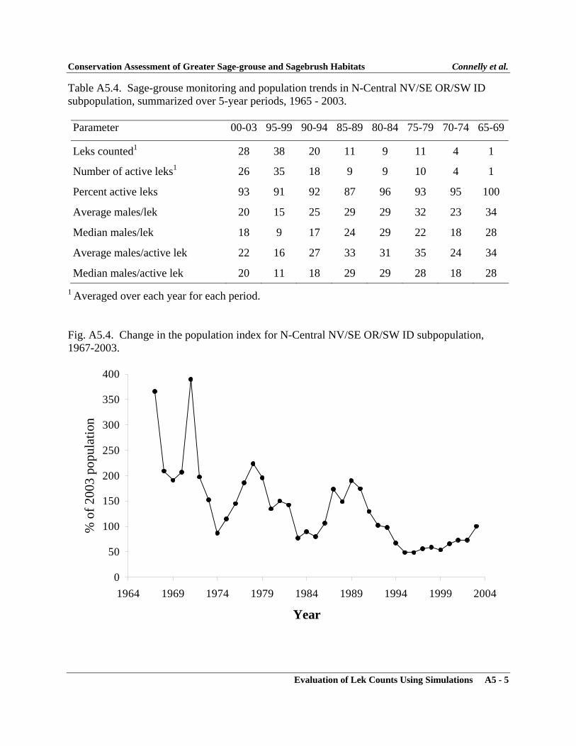
Conservation Assessment of Greater Sage-grouse and Sagebrush Habitats Connelly et al.
Evaluation of Lek Counts Using Simulations A5 - 5
Table A5.4. Sage-grouse monitoring and population trends in N-Central NV/SE OR/SW ID subpopulation, summarized over 5-year periods, 1965 - 2003. Parameter 00-03 95-99 90-94 85-89 80-84 75-79 70-74 65-69
Leks counted1 28 38 20 11 9 11 4 1
Number of active leks1 26 35 18 9 9 10 4 1
Percent active leks 93 91 92 87 96 93 95 100
Average males/lek 20 15 25 29 29 32 23 34
Median males/lek 18 9 17 24 29 22 18 28
Average males/active lek 22 16 27 33 31 35 24 34
Median males/active lek 20 11 18 29 29 28 18 28 1 Averaged over each year for each period. Fig. A5.4. Change in the population index for N-Central NV/SE OR/SW ID subpopulation, 1967-2003.
0
50
100
150
200
250
300
350
400
1964 1969 1974 1979 1984 1989 1994 1999 2004
Year
% o
f 200
3 po
pula
tion

Conservation Assessment of Greater Sage-grouse and Sagebrush Habitats Connelly et al.
Evaluation of Lek Counts Using Simulations A5 - 6
Table A5.5. Sage-grouse monitoring and population trends in NE NV/S-Central ID/NW UT subpopulation, summarized over 5-year periods, 1965 - 2003. Parameter 00-03 95-99 90-94 85-89 80-84 75-79 70-74 65-69
Leks counted1 179 118 57 57 87 51 47 25
Number of active leks1 145 89 48 39 70 46 38 23
Percent active leks 81 76 84 68 81 90 81 90
Average males/lek 15 13 20 21 22 28 24 31
Median males/lek 9 7 14 10 12 17 15 21
Average males/active lek 19 17 23 31 27 31 29 34
Median males/active lek 14 12 18 24 17 20 19 24 1 Averaged over each year for each period. Fig. A5.5. Change in the population index for NE NV/S-Central ID/NW UT subpopulation, 1965-2003.
0
50
100
150
200
250
300
350
400
1964 1969 1974 1979 1984 1989 1994 1999 2004
Year
% o
f 200
3 po
pula
tion

Conservation Assessment of Greater Sage-grouse and Sagebrush Habitats Connelly et al.
Evaluation of Lek Counts Using Simulations A5 - 7
Table A5.6. Sage-grouse monitoring and population trends in S-Central OR/N-Central NV subpopulation, summarized over 5-year periods, 1965 - 2003. Parameter 00-03 95-99 90-94 85-89 80-84 75-79 70-74 65-69
Leks counted1 1 4 1 0 0 0 0 0
Number of active leks1 1 4 1 0 0 0 0 0
Percent active leks 67 95 100
Average males/lek 2 8 16
Median males/lek 1 5 17
Average males/active lek 3 8 16
Median males/active lek 3 5 17 1 Averaged over each year for each period.

Conservation Assessment of Greater Sage-grouse and Sagebrush Habitats Connelly et al.
Evaluation of Lek Counts Using Simulations A5 - 8
Table A5.7. Sage-grouse monitoring and population trends in SE NV/SW UT subpopulation, summarized over 5-year periods, 1965 - 2003. Parameter 00-03 95-99 90-94 85-89 80-84 75-79 70-74 65-69
Leks counted1 68 38 35 32 33 14 10 1
Number of active leks1 52 37 35 31 33 11 8 1
Percent active leks 77 97 98 98 99 77 88 100
Average males/lek 12 12 15 15 18 12 24 24
Median males/lek 9 9 10 12 13 7 18 22
Average males/active lek 15 12 15 16 19 16 28 24
Median males/active lek 11 10 11 13 13 12 23 22 1 Averaged over each year for each period. Fig. A5.6. Change in the population index for SE NV/SW UT subpopulation, 1970-2003.
0
50
100
150
200
250
300
350
400
450
500
1969 1974 1979 1984 1989 1994 1999 2004
Year
% o
f 200
3 po
pula
tion
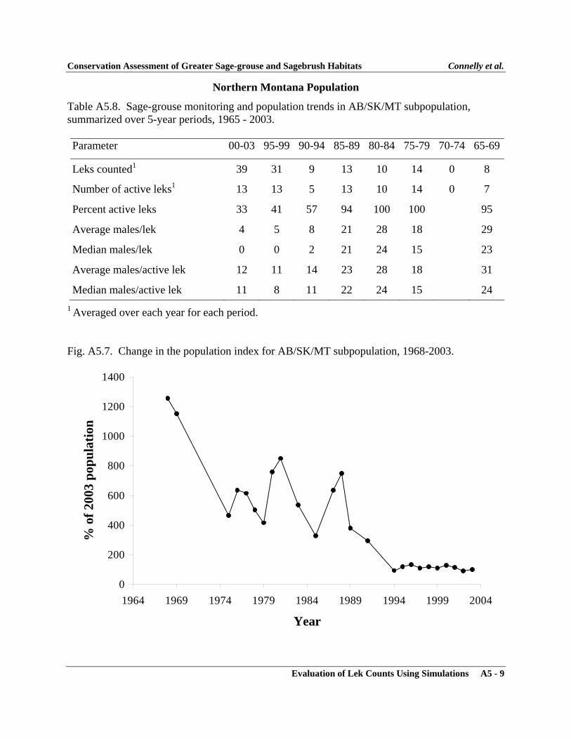
Conservation Assessment of Greater Sage-grouse and Sagebrush Habitats Connelly et al.
Evaluation of Lek Counts Using Simulations A5 - 9
Northern Montana Population
Table A5.8. Sage-grouse monitoring and population trends in AB/SK/MT subpopulation, summarized over 5-year periods, 1965 - 2003. Parameter 00-03 95-99 90-94 85-89 80-84 75-79 70-74 65-69
Leks counted1 39 31 9 13 10 14 0 8
Number of active leks1 13 13 5 13 10 14 0 7
Percent active leks 33 41 57 94 100 100 95
Average males/lek 4 5 8 21 28 18 29
Median males/lek 0 0 2 21 24 15 23
Average males/active lek 12 11 14 23 28 18 31
Median males/active lek 11 8 11 22 24 15 24 1 Averaged over each year for each period. Fig. A5.7. Change in the population index for AB/SK/MT subpopulation, 1968-2003.
0
200
400
600
800
1000
1200
1400
1964 1969 1974 1979 1984 1989 1994 1999 2004
Year
% o
f 200
3 po
pula
tion

Conservation Assessment of Greater Sage-grouse and Sagebrush Habitats Connelly et al.
Evaluation of Lek Counts Using Simulations A5 - 10
Table A5.9. Sage-grouse monitoring and population trends in N-Central MT subpopulation, summarized over 5-year periods, 1965 - 2003. Parameter 00-03 95-99 90-94 85-89 80-84 75-79 70-74 65-69
Leks counted1 99 18 11 8 5 4 2 2
Number of active leks1 87 17 11 8 5 4 2 2
Percent active leks 88 94 100 98 100 100 100 100
Average males/lek 27 18 20 18 26 19 28 28
Median males/lek 22 16 18 15 25 22 28 25
Average males/active lek 31 19 20 18 26 19 28 28
Median males/active lek 26 17 18 16 25 22 28 25 1 Averaged over each year for each period. Fig. A5.8. Change in the population index for N-Central MT subpopulation, 1965-2003.
0
50
100
150
200
250
300
350
400
1964 1969 1974 1979 1984 1989 1994 1999 2004
Year
% o
f 200
3 po
pula
tion

Conservation Assessment of Greater Sage-grouse and Sagebrush Habitats Connelly et al.
Evaluation of Lek Counts Using Simulations A5 - 11
Table A5.10. Sage-grouse monitoring and population trends in S-Central SK/MT subpopulation, summarized over 5-year periods, 1965 - 2003. Parameter 00-03 95-99 90-94 85-89 80-84 75-79 70-74 65-69
Leks counted1 18 14 4 7 0 0 0 0
Number of active leks1 14 7 2 7 0 0 0 0
Percent active leks 78 48 41 92
Average males/lek 10 6 3 30
Median males/lek 10 0 0 24
Average males/active lek 13 12 6 33
Median males/active lek 12 11 3 26 1 Averaged over each year for each period. Fig. A5.9. Change in the population index for S-Central SK/MT subpopulation, 1987-2003.
0
200
400
600
800
1000
1200
1400
1600
1986 1988 1990 1992 1994 1996 1998 2000 2002 2004
Year
% o
f 200
3 po
pula
tion

Conservation Assessment of Greater Sage-grouse and Sagebrush Habitats Connelly et al.
Evaluation of Lek Counts Using Simulations A5 - 12
Snake, Salmon, and Beaverhead Population
Table A5.11. Sage-grouse monitoring and population trends in Big Lost ID subpopulation, summarized over 5-year periods, 1965 - 2003. Parameter 00-03 95-99 90-94 85-89 80-84 75-79 70-74 65-69
Leks counted1 12 8 1 1 4 1 3 0
Number of active leks1 11 6 1 1 4 1 3 0
Percent active leks 91 82 71 100 90 100 100 100
Average males/lek 17 12 6 12 22 47 54 97
Median males/lek 13 8 3 12 19 30 50 97
Average males/active lek 19 15 9 12 24 47 54 97
Median males/active lek 17 11 4 12 20 30 50 97 1 Averaged over each year for each period. Fig. A5.10. Change in the population index for Big Lost ID subpopulation, 1969-2003.
0
50
100
150
200
250
300
350
400
450
500
1968 1972 1976 1980 1984 1988 1992 1996 2000 2004
Year
% o
f 200
3 po
pula
tion

Conservation Assessment of Greater Sage-grouse and Sagebrush Habitats Connelly et al.
Evaluation of Lek Counts Using Simulations A5 - 13
Table A5.12. Sage-grouse monitoring and population trends in Lemhi-Birch ID subpopulation, summarized over 5-year periods, 1965 - 2003. Parameter 00-03 95-99 90-94 85-89 80-84 75-79 70-74 65-69
Leks counted1 19 14 13 12 5 7 6 6
Number of active leks1 12 7 10 11 4 5 6 5
Percent active leks 61 51 72 98 79 67 97 93
Average males/lek 13 8 16 28 12 13 20 29
Median males/lek 6 1 9 19 11 4 18 30
Average males/active lek 21 16 22 28 15 20 21 31
Median males/active lek 16 14 14 19 18 16 18 32 1 Averaged over each year for each period. Fig. A5.11. Change in the population index for Lemhi-Birch ID subpopulation, 1965-2003.
0
50
100
150
200
250
300
1964 1969 1974 1979 1984 1989 1994 1999 2004
Year
% o
f 200
3 po
pula
tion

Conservation Assessment of Greater Sage-grouse and Sagebrush Habitats Connelly et al.
Evaluation of Lek Counts Using Simulations A5 - 14
Table A5.13. Sage-grouse monitoring and population trends in Little Lost ID subpopulation, summarized over 5-year periods, 1965 - 2003. Parameter 00-03 95-99 90-94 85-89 80-84 75-79 70-74 65-69
Leks counted1 11 5 4 3 2 2 4 2
Number of active leks1 10 4 4 2 2 1 3 2
Percent active leks 95 80 95 80 73 70 78 100
Average males/lek 34 26 30 30 17 16 38 32
Median males/lek 26 18 28 27 8 14 12 19
Average males/active lek 36 32 31 38 23 23 49 32
Median males/active lek 27 35 29 37 9 17 42 19 1 Averaged over each year for each period. Fig. A5.12. Change in the population index for Little Lost ID subpopulation, 1973-2003.
0
50
100
150
200
250
300
1972 1977 1982 1987 1992 1997 2002
Year
% o
f 200
3 po
pula
tion

Conservation Assessment of Greater Sage-grouse and Sagebrush Habitats Connelly et al.
Evaluation of Lek Counts Using Simulations A5 - 15
Table A5.14. Sage-grouse monitoring and population trends in N Side Snake ID subpopulation, summarized over 5-year periods, 1965 - 2003. Parameter 00-03 95-99 90-94 85-89 80-84 75-79 70-74 65-69
Leks counted1 13 9 12 12 8 7 6 4
Number of active leks1 12 6 10 10 6 6 6 4
Percent active leks 90 67 88 83 67 83 90 95
Average males/lek 17 13 23 22 25 28 33 32
Median males/lek 11 10 22 18 19 14 26 23
Average males/active lek 19 19 27 26 37 33 36 33
Median males/active lek 13 13 23 23 33 24 32 24 1 Averaged over each year for each period. Fig. A5.13. Change in the population index for N Side Snake ID subpopulation, 1965-2003.
0
50
100
150
200
250
300
1964 1969 1974 1979 1984 1989 1994 1999 2004
Year
% o
f 200
3 po
pula
tion
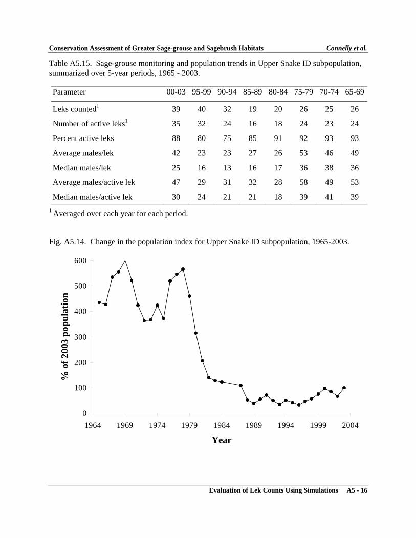
Conservation Assessment of Greater Sage-grouse and Sagebrush Habitats Connelly et al.
Evaluation of Lek Counts Using Simulations A5 - 16
Table A5.15. Sage-grouse monitoring and population trends in Upper Snake ID subpopulation, summarized over 5-year periods, 1965 - 2003. Parameter 00-03 95-99 90-94 85-89 80-84 75-79 70-74 65-69
Leks counted1 39 40 32 19 20 26 25 26
Number of active leks1 35 32 24 16 18 24 23 24
Percent active leks 88 80 75 85 91 92 93 93
Average males/lek 42 23 23 27 26 53 46 49
Median males/lek 25 16 13 16 17 36 38 36
Average males/active lek 47 29 31 32 28 58 49 53
Median males/active lek 30 24 21 21 18 39 41 39 1 Averaged over each year for each period. Fig. A5.14. Change in the population index for Upper Snake ID subpopulation, 1965-2003.
0
100
200
300
400
500
600
1964 1969 1974 1979 1984 1989 1994 1999 2004
Year
% o
f 200
3 po
pula
tion

Conservation Assessment of Greater Sage-grouse and Sagebrush Habitats Connelly et al.
Evaluation of Lek Counts Using Simulations A5 - 17
Wyoming Basin Population Table A5.16. Sage-grouse monitoring and population trends in Dinosaur UT/CO subpopulation, summarized over 5-year periods, 1965 - 2003. Parameter 00-03 95-99 90-94 85-89 80-84 75-79 70-74 65-69
Leks counted1 27 19 17 13 8 9 9 5
Number of active leks1 18 17 14 11 6 8 7 4
Percent active leks 69 86 86 82 79 93 84 96
Average males/lek 23 29 20 17 21 34 24 51
Median males/lek 7 13 11 11 12 15 15 34
Average males/active lek 33 34 23 21 26 37 29 53
Median males/active lek 18 19 12 14 16 16 16 40 1 Averaged over each year for each period. Fig. A5.15. Change in the population index for Dinosaur UT/CO subpopulation, 1965-2003.
0
100
200
300
400
500
600
1964 1969 1974 1979 1984 1989 1994 1999 2004
Year
% o
f 199
6 po
pula
tion

Conservation Assessment of Greater Sage-grouse and Sagebrush Habitats Connelly et al.
Evaluation of Lek Counts Using Simulations A5 - 18
Table A5.17. Sage-grouse monitoring and population trends in Fall River SD/E Edge WY subpopulation, summarized over 5-year periods, 1965 - 2003. Parameter 00-03 95-99 90-94 85-89 80-84 75-79 70-74 65-69
Leks counted1 5 1 1 1 2 0 0 0
Number of active leks1 5 1 1 1 2 0 0 0
Percent active leks 100 100 100 100 100
Average males/lek 16 9 7 6 25
Median males/lek 8 9 6
Average males/active lek 16 9 7 6 25
Median males/active lek 8 9 6 1 Averaged over each year for each period. Fig. A5.16. Change in the population index for Fall River SD/E Edge WY subpopulation, 1982-2003.
0
400
800
1200
1600
2000
2400
1980 1984 1988 1992 1996 2000 2004
Year
% o
f 200
3 po
pula
tion

Conservation Assessment of Greater Sage-grouse and Sagebrush Habitats Connelly et al.
Evaluation of Lek Counts Using Simulations A5 - 19
Table A5.18. Sage-grouse monitoring and population trends in NE WY/SE MT subpopulation, summarized over 5-year periods, 1965 - 2003. Parameter 00-03 95-99 90-94 85-89 80-84 75-79 70-74 65-69
Leks counted1 197 87 77 76 78 25 15 7
Number of active leks1 132 52 56 62 71 23 15 7
Percent active leks 67 59 73 81 92 91 97 100
Average males/lek 11 8 13 16 22 25 23 36
Median males/lek 6 3 8 11 17 19 20 31
Average males/active lek 17 14 18 20 24 28 24 36
Median males/active lek 12 10 13 15 18 21 21 31 1 Averaged over each year for each period. Fig. A5.17. Change in the population index for NE WY/SE MT subpopulation, 1967-2003.
0
200
400
600
800
1000
1200
1400
1964 1969 1974 1979 1984 1989 1994 1999 2004
Year
% o
f 200
3 po
pula
tion
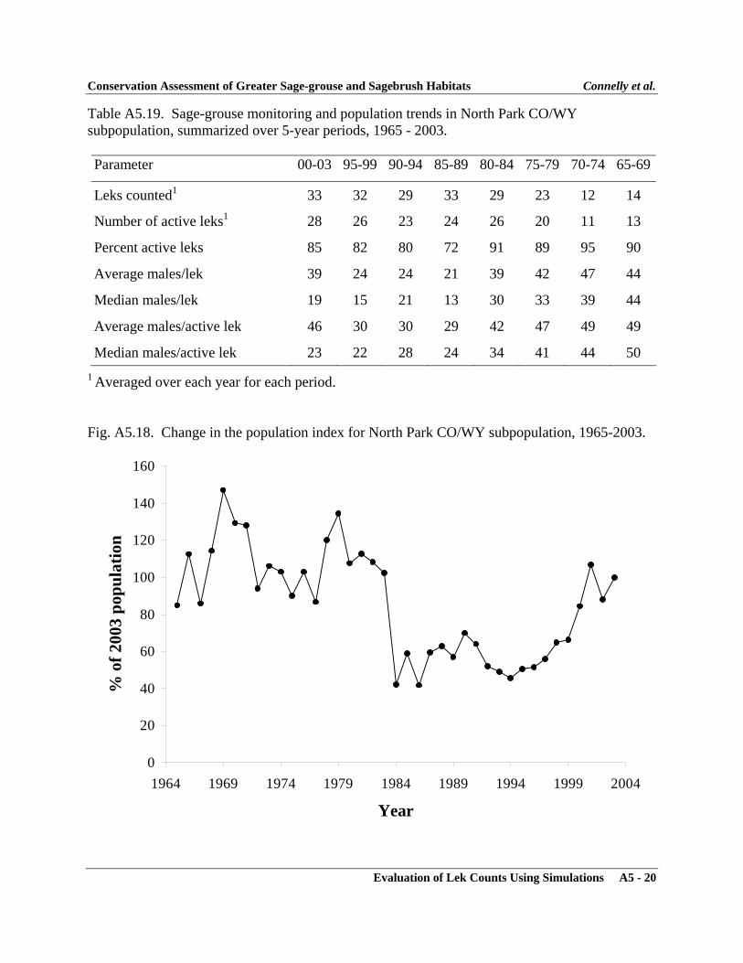
Conservation Assessment of Greater Sage-grouse and Sagebrush Habitats Connelly et al.
Evaluation of Lek Counts Using Simulations A5 - 20
Table A5.19. Sage-grouse monitoring and population trends in North Park CO/WY subpopulation, summarized over 5-year periods, 1965 - 2003. Parameter 00-03 95-99 90-94 85-89 80-84 75-79 70-74 65-69
Leks counted1 33 32 29 33 29 23 12 14
Number of active leks1 28 26 23 24 26 20 11 13
Percent active leks 85 82 80 72 91 89 95 90
Average males/lek 39 24 24 21 39 42 47 44
Median males/lek 19 15 21 13 30 33 39 44
Average males/active lek 46 30 30 29 42 47 49 49
Median males/active lek 23 22 28 24 34 41 44 50 1 Averaged over each year for each period. Fig. A5.18. Change in the population index for North Park CO/WY subpopulation, 1965-2003.
0
20
40
60
80
100
120
140
160
1964 1969 1974 1979 1984 1989 1994 1999 2004
Year
% o
f 200
3 po
pula
tion

Conservation Assessment of Greater Sage-grouse and Sagebrush Habitats Connelly et al.
Evaluation of Lek Counts Using Simulations A5 - 21
Table A5.20. Sage-grouse monitoring and population trends in S-Central MT/N-Central WY subpopulation, summarized over 5-year periods, 1965 - 2003. Parameter 00-03 95-99 90-94 85-89 80-84 75-79 70-74 65-69
Leks counted1 159 114 108 93 68 30 24 20
Number of active leks1 133 86 85 78 62 25 14 6
Percent active leks 84 75 78 83 91 82 57 28
Average males/lek 16 13 15 16 19 18 12 8
Median males/lek 12 9 10 11 14 15 4 0
Average males/active lek 19 17 19 19 21 22 20 26
Median males/active lek 15 12 14 14 15 18 15 19 1 Averaged over each year for each period. Fig. A5.19. Change in the population index for S-Central MT/N-Central WY subpopulation, 1969-2003.
0
50
100
150
200
250
300
1964 1969 1974 1979 1984 1989 1994 1999 2004
Year
% o
f 200
3 po
pula
tion

Conservation Assessment of Greater Sage-grouse and Sagebrush Habitats Connelly et al.
Evaluation of Lek Counts Using Simulations A5 - 22
Table A5.21. Sage-grouse monitoring and population trends in S-Central WY/N-Central CO subpopulation, summarized over 5-year periods, 1965 - 2003. Parameter 00-03 95-99 90-94 85-89 80-84 75-79 70-74 65-69
Leks counted1 491 372 283 268 199 106 66 81
Number of active leks1 323 225 180 174 118 70 52 64
Percent active leks 66 60 63 65 59 66 79 79
Average males/lek 20 12 15 16 20 27 32 41
Median males/lek 11 5 8 10 8 16 24 27
Average males/active lek 31 19 23 25 34 41 41 51
Median males/active lek 25 14 18 20 26 34 32 36 1 Averaged over each year for each period. Fig. A5.20. Change in the population index for S-Central WY/N-Central CO subpopulation, 1965-2003.
0
50
100
150
200
250
300
350
400
450
500
1964 1969 1974 1979 1984 1989 1994 1999 2004
Year
% o
f 200
3 po
pula
tion

Conservation Assessment of Greater Sage-grouse and Sagebrush Habitats Connelly et al.
Evaluation of Lek Counts Using Simulations A5 - 23
Table A5.22. Sage-grouse monitoring and population trends in SW WY/NW CO/NE UT/SE ID subpopulation, summarized over 5-year periods, 1965 - 2003. Parameter 00-03 95-99 90-94 85-89 80-84 75-79 70-74 65-69
Leks counted1 282 207 166 100 58 31 17 10
Number of active leks1 203 132 95 79 53 26 15 9
Percent active leks 72 64 57 79 92 86 84 86
Average males/lek 22 18 14 22 26 38 29 34
Median males/lek 15 8 5 16 19 21 21 26
Average males/active lek 31 28 25 28 28 44 34 39
Median males/active lek 24 20 19 22 20 29 26 31 1 Averaged over each year for each period. Fig. A5.21. Change in the population index for SW WY/NW CO/NE UT/SE ID subpopulation, 1965-2003.
0
20
40
60
80
100
120
140
160
180
200
1964 1969 1974 1979 1984 1989 1994 1999 2004
Year
% o
f 200
3 po
pula
tion

Conservation Assessment of Greater Sage-grouse and Sagebrush Habitats Connelly et al.
Evaluation of Lek Counts Using Simulations A5 - 24
Yellowstone Watershed Population Table A5.23. Sage-grouse monitoring and population trends in Central MT subpopulation, summarized over 5-year periods, 1965 - 2003. Parameter 00-03 95-99 90-94 85-89 80-84 75-79 70-74 65-69
Leks counted1 239 111 95 116 96 75 52 8
Number of active leks1 175 79 72 94 88 67 47 8
Percent active leks 73 71 76 81 91 90 91 97
Average males/lek 17 14 16 17 27 23 23 23
Median males/lek 12 10 11 13 23 19 18 14
Average males/active lek 24 20 21 21 30 25 25 23
Median males/active lek 19 16 15 16 26 21 20 15 1 Averaged over each year for each period. Fig. A5.22. Change in the population index for Central MT subpopulation, 1966-2003.
0
50
100
150
200
250
300
1964 1969 1974 1979 1984 1989 1994 1999 2004
Year
% o
f 200
3 po
pula
tion

Conservation Assessment of Greater Sage-grouse and Sagebrush Habitats Connelly et al.
Evaluation of Lek Counts Using Simulations A5 - 25
Table A5.24. Sage-grouse monitoring and population trends in E Interior MT/NE tip WY subpopulation, summarized over 5-year periods, 1965 - 2003. Parameter 00-03 95-99 90-94 85-89 80-84 75-79 70-74 65-69
Leks counted1 102 19 35 23 32 13 2 0
Number of active leks1 61 10 24 15 28 13 2 0
Percent active leks 60 53 69 66 88 97 100 100
Average males/lek 9 4 9 8 15 14 18 32
Median males/lek 3 2 7 6 13 11 20 32
Average males/active lek 15 8 13 13 17 14 18 32
Median males/active lek 10 7 12 10 14 12 20 32 1 Averaged over each year for each period. Fig. A5.23. Change in the population index for E Interior MT/NE tip WY subpopulation, 1974-2003.
0
100
200
300
400
500
600
1972 1976 1980 1984 1988 1992 1996 2000 2004
Year
% o
f 200
3 po
pula
tion

Evaluation of Lek Counts Using Simulations A6 - 1
APPENDIX 6
Characteristics of Greater Sage-Grouse Within Floristic Regions
Methods
The identified populations (Table 6.16, Appendix 4) and subpopulations (Table 6.16, Appendix 5) were divided into six floristic regions (Miller and Eddleman 2001) for a general analysis. An additional Great Plains Region was defined to include populations east and north of the area encompassed by Miller and Eddleman’s research. Because some populations/subpopulations straddled the lines between floristic regions, they were included within the region where they had most of their leks.
Literature Cited
Miller, R. F., and L. L. Eddleman. 2001. Spatial and temporal changes of sage grouse habitat in
the sagebrush biome. Oregon State University, Agricultural Experiment Station, Technical Bulletin 151, Corvallis, Oregon.

Conservation Assessment of Greater Sage-grouse and Sagebrush Habitats Connelly et al.
Evaluation of Lek Counts Using Simulations A6 - 2
Table A6.1. Sage-grouse monitoring and population trends in Colorado Plateau region, summarized over 5-year periods, 1965 - 2003. Parameter 00-03 95-99 90-94 85-89 80-84 75-79 70-74 65-69
Leks counted1 4 7 10 12 9 1 2 2
Number of active leks1 3 6 4 4 7 1 1 1
Percent active leks 80 86 39 34 78 67 67 63
Average males/lek 11 9 4 5 6 10 8 3
Median males/lek 8 5 0 0 5 10 5 3
Average males/active lek 14 11 10 14 8 14 12 5
Median males/active lek 13 7 8 11 6 13 8 5 1 Averaged over each year for each period. Fig. A6.1. Change in the population index for Colorado Plateau region, 1980-2003.
0
100
200
300
400
500
600
1976 1980 1984 1988 1992 1996 2000 2004
Year
% o
f 200
3 po
pula
tion

Conservation Assessment of Greater Sage-grouse and Sagebrush Habitats Connelly et al.
Evaluation of Lek Counts Using Simulations A6 - 3
Table A6.2. Sage-grouse monitoring and regional trends in Columbia Basin region, summarized over 5-year periods, 1965 - 2003. Parameter 00-03 95-99 90-94 85-89 80-84 75-79 70-74 65-69
Leks counted1 47 31 25 20 18 15 14 3
Number of active leks1 20 18 16 14 16 14 13 3
Percent active leks 41 56 62 71 91 92 99 100
Average males/lek 8 11 13 17 26 15 24 33
Median males/lek 0 5 4 6 23 13 20 31
Average males/active lek 18 20 20 23 28 16 25 33
Median males/active lek 17 18 14 14 24 14 20 31 1 Averaged over each year for each period. Fig. A6.2. Change in the population index for Columbia Basin region, 1965-2003.
0
100
200
300
400
500
600
700
1964 1969 1974 1979 1984 1989 1994 1999 2004
Year
% o
f 200
3 po
pula
tion

Conservation Assessment of Greater Sage-grouse and Sagebrush Habitats Connelly et al.
Evaluation of Lek Counts Using Simulations A6 - 4
Table A6.3. Sage-grouse monitoring and regional trends in Great Plains region, summarized over 5-year periods, 1965 - 2003. Parameter 00-03 95-99 90-94 85-89 80-84 75-79 70-74 65-69
Leks counted1 747 315 271 274 255 158 94 44
Number of active leks1 519 203 203 224 232 145 87 42
Percent active leks 69 64 75 82 91 92 93 94
Average males/lek 15 10 13 16 22 20 21 22
Median males/lek 9 5 9 11 17 16 18 16
Average males/active lek 21 16 18 20 25 22 23 23
Median males/active lek 16 12 13 15 20 18 20 18 1 Averaged over each year for each period. Fig. A6.3. Change in the population index for Great Plains region, 1965-2003.
0
50
100
150
200
250
300
350
400
1964 1969 1974 1979 1984 1989 1994 1999 2004
Year
% o
f 200
3 po
pula
tion

Conservation Assessment of Greater Sage-grouse and Sagebrush Habitats Connelly et al.
Evaluation of Lek Counts Using Simulations A6 - 5
Table A6.4. Sage-grouse monitoring and regional trends in Northern Great Basin region, summarized over 5-year periods, 1965 - 2003. Parameter 00-03 95-99 90-94 85-89 80-84 75-79 70-74 65-69
Leks counted1 18 32 22 33 48 72 107 156
Number of active leks1 16 25 11 25 44 64 92 127
Percent active leks 91 79 50 76 91 88 86 82
Average males/lek 23 21 9 19 29 30 19 22
Median males/lek 14 11 1 10 19 17 12 13
Average males/active lek 25 26 17 25 32 34 22 27
Median males/active lek 16 16 14 17 20 20 15 19 1 Averaged over each year for each period. Fig. A6.4. Change in the population index for Northern Great Basin region, 1965-2003.
0
50
100
150
200
250
300
350
400
450
1964 1969 1974 1979 1984 1989 1994 1999 2004
Year
% o
f 200
3 po
pula
tion

Conservation Assessment of Greater Sage-grouse and Sagebrush Habitats Connelly et al.
Evaluation of Lek Counts Using Simulations A6 - 6
Table A6.5. Sage-grouse monitoring and regional trends in Snake River Basin region, summarized over 5-year periods, 1965 - 2003. Parameter 00-03 95-99 90-94 85-89 80-84 75-79 70-74 65-69
Leks counted1 450 334 195 169 215 172 149 97
Number of active leks1 364 256 158 136 177 155 130 91
Percent active leks 81 77 81 81 83 90 87 93
Average males/lek 20 15 21 28 22 32 31 39
Median males/lek 13 9 14 18 14 21 21 29
Average males/active lek 25 20 26 34 27 36 36 42
Median males/active lek 18 15 18 25 18 24 26 30 1 Averaged over each year for each period. Fig. A6.5. Change in the population index for Snake River Basin region, 1965-2003.
0
50
100
150
200
250
300
1964 1969 1974 1979 1984 1989 1994 1999 2004
Year
% o
f 200
3 po
pula
tion

Conservation Assessment of Greater Sage-grouse and Sagebrush Habitats Connelly et al.
Evaluation of Lek Counts Using Simulations A6 - 7
Table A6.6. Sage-grouse monitoring and regional trends in Southern Great Basin region, summarized over 5-year periods, 1965 - 2003. Parameter 00-03 95-99 90-94 85-89 80-84 75-79 70-74 65-69
Leks counted1 213 128 121 113 112 98 81 42
Number of active leks1 166 106 107 99 97 82 69 38
Percent active leks 78 83 89 87 87 83 85 90
Average males/lek 17 15 17 20 20 21 24 25
Median males/lek 10 10 11 14 14 13 16 16
Average males/active lek 22 18 19 23 23 25 28 28
Median males/active lek 15 13 14 16 17 18 22 19 1 Averaged over each year for each period. Fig. A6.6. Change in the population index for Southern Great Basin region, 1965-2003.
0
50
100
150
200
250
300
1964 1969 1974 1979 1984 1989 1994 1999 2004
Year
% o
f 200
3 po
pula
tion

Conservation Assessment of Greater Sage-grouse and Sagebrush Habitats Connelly et al.
Evaluation of Lek Counts Using Simulations A6 - 8
Table A6.7. Sage-grouse monitoring and regional trends in Wyoming Basin region, summarized over 5-year periods, 1965 - 2003. Parameter 00-03 95-99 90-94 85-89 80-84 75-79 70-74 65-69
Leks counted1 1229 1100 819 693 587 381 287 242
Number of active leks1 892 751 565 511 449 312 237 199
Percent active leks 73 68 69 74 76 82 83 82
Average males/lek 20 15 16 20 22 30 30 37
Median males/lek 12 7 8 11 13 18 19 21
Average males/active lek 28 21 24 27 29 37 36 45
Median males/active lek 22 15 17 19 22 28 27 33 1 Averaged over each year for each period. Fig. A6.7. Change in the population index for Wyoming Basin region, 1965-2003.
0
50
100
150
200
250
300
350
400
450
1964 1969 1974 1979 1984 1989 1994 1999 2004
Year
% o
f 200
3 po
pula
tion