consensus between gcm climate change projections with empirical downscaling: precipitation...

INTERNATIONAL JOURNAL OF CLIMATOLOGY

Int. J. Climatol. 26: 1315–1337 (2006)

Published online 21 March 2006 in Wiley InterScience (www.interscience.wiley.com). DOI: 10.1002/joc.1314

CONSENSUS BETWEEN GCM CLIMATE CHANGE PROJECTIONS WITHEMPIRICAL DOWNSCALING: PRECIPITATION DOWNSCALING OVER

SOUTH AFRICA

B. C. HEWITSONa,* and R. G. CRANEb

a Climate System Analysis Group, Department Environmental and Geographical Science, University of Cape Town, Private Bag,Rondebosch 7701, South Africa

b Alliance for Earth Science, Engineering, Development in Africa, Earth and Mineral Science College, Pennsylvania State University,University Park, PA 16801, USA

Received 8 June 2005Revised 21 December 2005

Accepted 21 December 2005

ABSTRACT

This paper discusses issues that surround the development of empirical downscaling techniques as context for presentinga new approach based on self-organizing maps (SOMs). The technique is applied to the downscaling of daily precipitationover South Africa. SOMs are used to characterize the state of the atmosphere on a localized domain surrounding eachtarget location on the basis of NCEP 6-hourly reanalysis data from 1979 to 2002, and using surface and 700-hPa u andv wind vectors, specific and relative humidities, and surface temperature. Each unique atmospheric state is associatedwith an observed precipitation probability density function (PDF). Future climate states are derived from three globalclimate models (GCMs): HadAM3, ECHAM4.5, CSIRO Mk2. In each case, the GCM data are mapped to the NCEPSOMs for each target location and a precipitation value is drawn at random from the associated precipitation PDF. Thedownscaling approach combines the advantages of a direct transfer function and a stochastic weather generator, andprovides an indication of the strength of the regional versus stochastic forcing, as well as a measure of stationarity inthe atmosphere–precipitation relationship.

The methodology is applied to South Africa. The downscaling reveals a similarity in the projected climate changebetween the models. Each GCM projects similar changes in atmospheric state and they converge on a downscaled solutionthat points to increased summer rainfall in the interior and the eastern part of the country, and a decrease in winter rainfallin the Western Cape. The actual GCM precipitation projections from the three models show large areas of intermodeldisagreement, suggesting that the model differences may be due to their precipitation parameterization schemes, ratherthan to basic disagreements in their projections of the changing atmospheric state over South Africa. Copyright 2006Royal Meteorological Society.

KEY WORDS: climate change; downscaling; self-organizing maps; global climate model; precipitation; South Africa

1. INTRODUCTION

Empirical downscaling is a widely used technique for exploring the regional and local-scale response toglobal climate change as simulated by comparatively low-resolution global climate models (GCMs). Asnoted in the third assessment report (TAR) of the intergovernmental panel on climate change (IPCC, 2001),downscaling has wide appeal because of its low computational needs and its relative ease of application.This makes it particularly attractive to the impacts community and especially to developing nations, and theapproach has been widely adopted. (See, e.g. the extensive references of the IPCC TGICA guidance documenton statistical (empirical) downscaling, from http://ipcc-ddc.cru.uea.ac.uk/guidelines/index.html.) For regionalclimate change projections, the TAR also concludes that empirical approaches have similar skill levels as

* Correspondence to: B. C. Hewitson, Department of Environmental and Geographical Science, University of Cape Town, Private Bag,Rondebosch 7701, South Africa; e-mail: [email protected]

Copyright 2006 Royal Meteorological Society

1316 B. C. HEWITSON AND R. G. CRANE

current implementations of numerical regional climate models (RCMs). While increasing in popularity, therehas been little discussion of the advantages and, more importantly, the limitations in using empirical techniquesfor climate downscaling. In this paper we discuss the basic assumptions that underlie this approach and presenta new technique that attempts to reduce these limitations in an empirical downscaling of daily precipitationover South Africa.

The TAR, however, also highlights the extensive and diverse list of empirical techniques that have beenapplied to climate downscaling (IPCC, 2001: Chapter 10, Appendix A), and the number has grown subsequentto the TAR publication. There has been little assessment of the strengths and weaknesses of the differentmethodological approaches. Many techniques are based on different statistical models, requiring differentassumptions concerning the input data, and subjective decisions on the choice of statistical parameters. Theoutputs may be strongly dependent on the atmospheric variables and the period of observation used. In somerespects, this has reduced clarity and confidence in the results, and limited the value of empirical downscalingfor the policy and impacts community – a community urgently in need of credible regional-scale scenariosof future climate. Regional Climate Models, while often perceived by the impacts community as an optimumapproach to downscaling GCMs, have their own problems in application. Most notable are the sensitivityand validation analyses necessary to select the optimum model and model parameterization schemes forthe particular region of interest, and the consequent issues of stationarity and tuning. Consequently, mostimpacts assessments still rely on GCM results (which are not very skillful at the spatial scales required)for their principal source information on future climate possibilities. While some regional-scale informationcontent can be crudely derived from GCMs (e.g. Hewitson, 2003), there is a continuing demand for robustdownscaling techniques that reflect a regional climate manifestation inherently consistent with the large-scale,GCM-simulated response of the climate system dynamics to anthropogenic forcing.

GCMs now have a history of intercomparison studies (e.g. Lambert and Boer, 2001; Achuta Rao andSperber, 2002; Covey et al., 2003) and there have been several recent initiatives to carry out similar studies forRCMs (e.g. Christensen et al., 2005). Although empirical downscaling algorithms can be broadly categorizedinto one of three or four major methodologies, there are varied implementations of these methodologies, andthere has been little attempt at systematic intercomparison studies. Wilby et al. (1998) began the processby contrasting several techniques, but the comparisons, so far, have been limited in scope and have notaddressed the broad spectrum of empirical techniques found in the literature. On the other hand, it could beargued that there is unlikely to be a ‘best’ downscaling algorithm, and that the optimum technique is likelyto be application- and region specific. There may not be much to be gained by an in-depth intercomparisonstudy, and it may be more important simply to clearly articulate the benefits and limitations of any particulardownscaled product for the user community.

What we present here is a downscaling procedure that utilizes the commonly accepted advantages of severaltechniques, while minimizing their limitations. The objectives are to:

(1) Present a discussion of what constitutes a robust downscaling application. This builds on previousdiscussions in the literature beginning with Hewitson and Crane (1996), where questions over the selectionof atmospheric predictors were explored, and continues more recently with the guidance documents onclimate change scenarios published by the IPCC Task Group on Impact Assessments (Wilby et al., 2004).

(2) Develop a downscaling algorithm that seeks to address these issues and which, if not completely, then tosome extent qualifies the remaining uncertainty. We suggest that this or similar approaches are requiredif the downscaled products are to be defensible, and of value to the policy and impacts communities.

(3) Apply the technique to a dense precipitation observational network in South Africa.(4) Derive a range of precipitation statistics that can have immediate application in the formulation of

adaptation and mitigation strategies in response to anthropogenic climate change in the region.

While assessing GCM performance was not a specific objective of the study, the results presented heresuggest that much of the discrepancy between GCM projections of precipitation over South Africa (at leastfor the three models used here) may be due to differences in parameterization schemes, rather than inherentdifferences in the GCM simulations of regional dynamics.

Copyright 2006 Royal Meteorological Society Int. J. Climatol. 26: 1315–1337 (2006)

EMPIRICAL DOWNSCALING CONSENSUS 1317

2. EMPIRICAL DOWNSCALING: ISSUES OF CONCERN

Before presenting a new methodology, and in the light of the diversity of approaches that currently exist andthe limited number of intercomparison studies, it is worth re-examining the basic principles and assumptionsof empirical downscaling. This provides the context for explaining the particular approach adopted here.Empirical downscaling is conceptually very simple and is based on the premise that the local-scale climateis in some measure a response to the larger, synoptic-scale forcing. Observational data are used to derivea relationship between the synoptic-scale and local climates, and that relationship can then be used withcomparable resolution fields of a GCM to generate information on the local climate consistent with the GCMforcing. The assumption that the local climate is conditioned by the larger-scale forcing is reasonable, evenwhere the local climate is governed by mesoscale events such as convective systems, as these are, in turn,conditional on the synoptic state.

2.1. Synoptic-scale versus local forcing

While it is true that the synoptic-scale forcing will have some influence on local climate, there is alsoa degree of local forcing that will vary by region and by season. This local forcing can be both fixed andvariable. Topography and land–water boundaries represent a fixed forcing for the local climate. The degree towhich that forcing impacts the local climate, however, is also a function of the larger-scale flow. Consequently,the effects of this local forcing can be readily incorporated in the downscaling transfer function if appropriatemeasures of flow direction, stability, etc. are included in the predictor variables.

Variable local forcing would include, for example, land use and land cover change. For some regions, thiscould have a major impact on local climates, which cannot be captured by empirical downscaling techniques.While there have been sensitivity studies with both GCMs and RCMs that examine the impacts of land coverchange (e.g. Taylor et al., 2002; Gao et al., 2003), we are not aware of any generally available RCMs thatinclude two-way interactive vegetation or land cover schemes, or include scenarios of changes in land usepractice. However, this is obviously something that should eventually be included in any RCM used forclimate change impacts analysis. While impacts analyses can examine possible land cover/land use changesas one of a set of multiple stressors, the degree to which land cover changes can feedback to impact localclimate represents an element of uncertainty in the climate projections analogous to, e.g. uncertainty due tofuture levels of greenhouse gas emissions.

In addition, for any synoptic state, there may be variation around a generalized response conditional on,for example, antecedent soil moisture. This small-scale variability is not captured by the GCM and theeffects, therefore, are not included in the transfer function. Depending on the spatial scale involved, some ofthese may be treated explicitly by RCMs. For both empirical downscaling and for sub-grid-scale processesin RCMs these variations become a stochastic permutation of the response to a given synoptic state andcan be modeled as such. Some downscaling methodologies are more appropriate for extracting the directsynoptic-scale forcing, while others are more effective at generating the stochastic element. At the same time,some techniques capture only the linear forcing, while others may capture any nonlinear forcing that may bepresent.

2.2. Stationarity

Given that there is a relationship between the larger-scale and the local climate, and assuming anappropriate downscaling transfer function can be generated, an empirical downscaling of present climate iseminently feasible. However, an additional factor becomes important when considering future climates – thatof stationarity of the downscaling function. It is not immediately obvious that a relationship derived for thepresent climate can be applied to a future climate state. Empirical downscaling implicitly assumes that theobservational data from which the relationship is developed encompasses the required information for futurecross-scale relationships. Essentially, this assumes that, for a given region, the same synoptic-scale states arepresent in the future and that climate change will, for the most part, manifest itself as a change in the timing,persistence, and frequency of these larger-scale events. While we cannot verify stationarity until after the



fact, we can at least make some assessment of the likelihood on the basis of the changes in the large-scaleclimate of the GCM.

More difficult to assess is the possibility that the nature of the transfer function itself will change in thefuture. In many respects, appropriate selection of atmospheric variables that fully encompass the physics ofthe large-scale forcing would obviate this. However, if a change signal is present in a variable not selected,this can result in the transfer function progressively becoming less appropriate. One possible example wouldbe if the concentration of cloud condensation nuclei significantly changes over a region. However, it is likelythat such effects will be secondary to changes attributable to the core circulation and humidity attributes of theatmosphere. The degree to which this is likely to be an issue will also depend on the time scales considered(the further we project into the future the more likely this is to be an issue) and on the choice of predictorvariables used.

2.3. Predictor variables

Past work (e.g. Hewitson and Crane, 1996; Cavazos and Hewitson, 2005) has shown that the choice ofpredictor variables is critical in capturing the anthropogenic climate change signal in the GCM. By using fieldsthat reflect the primary circulation dynamics of the atmosphere, one captures part of the synoptic-scale forcing.Neglecting the inclusion of some measure of atmospheric humidity as a predictor, however, could have anotable effect on a downscaled climate change precipitation signal (see Hewitson and Crane, 1996; Crane andHewitson, 1998). For a precipitation downscaling, including humidity not only improves the transfer functionpredictions for the present climate, but also reduces the stationarity issue noted above, as the dynamics and thehumidity fields become separate predictors in the downscaling function. From this perspective, it is essentialto have multiple predictor variables that have an understandable physical relationship to the downscaledparameter. Relationships that are purely correlative and for which there is no clear physical process linkageshould be avoided. For example, the El Nino southern oscillation (ENSO)–Africa teleconnection that inducesdrought in southern Africa during El Nino (e.g. Rautenbach and Smith, 2001) has shown indications ofweakening in recent years (Landman and Mason, 1999; Sewell and Landman, 2001). Consequently, there isno reason to expect that such teleconnection relationships will be maintained in future climates, and their useas predictors should be avoided.

2.4. Temporal resolution

A final issue is that of temporal resolution. Downscaling from time-mean fields is clearly feasible (see,for example, the discussion by Buishand et al., 2004). However, it is important to recognize that in someregions, climate change may be manifest as changes in the histogram of daily synoptic-scale events, with orwithout a change in the mean itself. Downscaling from time-averaged fields thus runs some risk of missingan important climate change signal.

In summary, the major issues to be addressed in any downscaling application should include:

(1) An assessment of the strength of the synoptic-scale forcing on any given variable for a given location – inother words, an assessment of the relative importance of synoptic-scale, local, and stochastic forcing, andof the degree to which the synoptic-scale forcing is linear versus nonlinear. In practice, this is mosteffectively accomplished through validation of the downscaling product. The degree to which the localclimate of a test data set is reproduced by the downscaling function is an indication of the relativestrengths of the large-scale versus local forcing.

(2) An assessment of the degree to which the future climate regime is reflected in the observational data usedto generate the relationship (i.e. the stationarity issue).

(3) The use of predictors that reflect the physical processes controlling the local climate response.(4) Downscaling at the time scale of daily weather events, even if these are to be subsequently aggregated

in some fashion for impacts analysis.

In addition, the utility of the final product will also depend on the GCM(s) used for the analysis, the qualityand duration of the observational network, and issues related to specific techniques (for example, assumptions



about data distributions that may be inherent in a particular statistical model). How all of these are addressedwill affect the quality and the reliability of the downscaled climate projections. In some cases, this assessmentprocess may indicate that a particular empirical downscaling approach is not viable for a region, application,or data set.

With these considerations in mind, we present a downscaling methodology that addresses each of theseissues and produces an effective regional climate change scenario for South Africa, within the constraints ofthe degree to which the large-scale climate change is captured by the GCMs used.

3. SELF-ORGANIZING MAPS

A self-organizing map (SOM) is a data description and visualization tool that extracts and displays the majorcharacteristics of the multidimensional data distribution function. SOMs are typically depicted as a two-dimensional array of nodes (although other topologies are possible), where each node is described by a vectorrepresenting the mean of the surrounding points in the multidimensional data space. In one respect, SOMsare similar to a ‘fuzzy’ clustering algorithm in which there are no distinct boundaries between groups, andindividual data points can contribute to the definition of more than one group. In other applications SOMscan be thought of as being analogous to obliquely rotated nonlinear empirical orthogonal functions (EOFs)or in another sense, a projection of the n-dimensional data space onto a two-dimensional array of generalizedmodes. SOMs were introduced by Kohonen (1989, 1990, 1991, 1995), and examples in the literature includetheir potential applications to synoptic climatology (Hewitson and Crane, 2002), precipitation regimes (Craneand Hewitson, 2003), and interpolation schemes (Hewitson and Crane, 2005). SOMs were used by Malmgrenand Winter (1999) and Cavazos (1999, 2000) for climate classification, by Hudson (1998) to examine synopticcirculation changes in GCM perturbation experiments, and by Ambroise et al. (2000) for cloud classification.Other related applications of SOMs are discussed in Cavazos and Hewitson (2005), Ni et al. (2002) andTennant (2003).

The SOMs are derived from an iterative training procedure. The SOM is a user-specified, two-dimensionalarray of nodes, each defined by a reference vector of length n. For a (n × m) data set where n is the numberof variables and m is the number of observations:

• We take the first observation and compare the observational vector to each of the node reference vectorsin the SOM (typically using Euclidean distance as the measure of similarity). The reference vector that isclosest to the observational vector is the ‘winning node’. The reference vector of the winning node is thenupdated, adjusting it slightly in the direction of the observational vector by a user-determined factor thatrepresents the ‘learning rate’. Too large a learning rate may lead to an unstable solution, while a smalllearning rate takes longer to converge on a solution. In practice, we start with a relatively small learningrate and decrease it further with subsequent iterations. Given that the computational needs are very modest(compared to an RCM) we simply set a small learning rate and an arbitrarily large (500 000) number ofiterations. Note that, unlike a feed-forward type of Artificial Neural Network, we are not fitting a function,and there is no issue of over-training or over-fitting with the SOM.

• All surrounding nodes are also updated, again being adjusted slightly (to a lesser degree than the winningnode) in the direction of the observational vector. The radius of nodes around the winning node that areupdated is determined by the ‘update kernel’ that decreases in radius during the iterative learning.

• Each observational vector is then presented to the SOM in turn and the procedure repeated for all of theobservations.

• The process is then repeated for multiple iterations until there is no change in the node assignment of eachobservation between iterations.

Typically, we assign random values to the initial node vectors, although other options are available (e.g.using the first two principal components of the data set). We also use a two stage process whereby we startwith a fairly large update kernel (close to the size of the smaller SOM dimension) for the first set of iterations.



Then using that final SOM as the starting point, we do a second training run with a smaller update kernel torefine the node definitions.

SOMs have some particularly advantageous characteristics from the point of view of climate downscaling:

• As noted above, each node reference vector is the n-dimensional mean of the nearby cloud of data points.The distribution of the SOM nodes in the data space is a function of data density and data similarity.The iterative training and the use of the update kernel result in similar observations mapping to nearbynodes, while observations that are very different to each other map to nodes that are located further apartin the SOM space. The SOM mapping, therefore, provides a simple and effective visualization of then-dimensional (and possibly nonlinear) data structure.

• More nodes are, after training, located in areas with greater data densities, and fewer nodes where there arefewer data points. Because the update kernel adjusts surrounding nodes during the training process, it ispossible that, if sufficient nodes are available (i.e. a large enough SOM), the SOM may also locate nodesin regions of the data space where there are no observations – in effect interpolating. The end result is thatthe SOM nodes represent archetypical points that span the continuum of the input data space.

• SOMs, unlike statistical models, make no assumptions about the underlying data, and the iterative trainingallows the SOM to describe any arbitrary linear or nonlinear data distribution function.

• The SOM is very effective at handling missing data in the observational vector. The comparison betweenthe observational vector and the node reference vector is based on matching pairs of vector elements, andthe SOM uses whichever pairs are available when computing the distance between the two vectors.

• The SOM gives consistent results regardless of the SOM dimensions used. The training procedure ensuresthat the most different patterns will move to opposite corners of the SOM array. As the array size increases,the same patterns are revealed, but with greater differentiation in the surrounding nodes. Large arrayspresent more detail in the pattern differentiations, while smaller arrays produce greater generalization – butthe underlying structure remains the same (e.g. Crane and Hewitson, 2003).

4. SOM-BASED DOWNSCALING

In essence, using observational data we apply SOMs to characterize the atmospheric circulation on a localizeddomain around the target location, and we generate probability density functions (PDFs) for the rainfalldistribution associated with each atmospheric state. For the downscaling we then take the GCM data, match itto the SOM characterization of the atmospheric states, and for each circulation state in the GCM data, randomlyselect precipitation values from the associated PDF. The general methodology is discussed in detail below.

4.1. Data

In this application we use daily mean atmospheric fields constructed from 6-hourly NCEP reanalysis datafor 1979 to 2002, restricting the range to post-1979 when the advent of satellite data for the reanalysissignificantly improved the quality of the reanalysis for the Southern Hemisphere (Tennant, 2004). The GCMdata are from simulations using the CSIRO Mk2, ECHAM4.5, and HadAM3 (using sea-surface temperatures(SST) from HadCM3) GCMs models, forced by the SRES A2 emissions scenario. As the GCM data to bedownscaled need to be of the same dimensions as the observational data, in this implementation the NCEPand GCM data are re-gridded to a common compromise grid of 3° × 3°. The data used to characterizethe atmosphere are comparable to the boundary conditions used to force an RCM, and include the u andv wind vectors (surface and at 700 hPa), temperature (surface), specific humidity (surface and at 700 hPa),and relative humidity (surface and 700 hPa). Both relative and specific humidity are included, as the formerreflects how close to saturation the atmosphere is, while the latter reflects the total water content.

A number of permutations of the mix of atmospheric variables and atmospheric levels were explored, andgenerally performed with comparable skill. Recognizing the high degree of correlation between variables andbetween levels in the atmosphere, the variables used here represent a common set that reflect the primary



circulation and water vapor attributes. As noted by Cavazos and Hewitson (2005), the most relevant genericvariables that should be selected as the base predictors for downscaling are those of mid-troposphere circulationand humidity. In addition, we include the surface variable, as it has been noted that in regions in whichorographic forcing plays a significant role, the surface data improve the characterization of the atmosphericstates that differentiate between precipitation regimes.

The precipitation data used are from a high-resolution, gridded data set for South Africa describedby Hewitson and Crane (2005). This data set has been created at both 0.1° and 0.25° resolutions froma source station observation data set of >3000 stations. The 0.25° resolution data set is used in thispaper, as it is comparable to the resolution of RCMs used in climate change downscaling applications.The interpolation methodology used (conditional interpolation) explicitly uses synoptic conditioning of theinterpolation parameters, and avoids or minimizes many of the problems inherent in interpolating a spatiallydiscontinuous field such a precipitation.

The location of the precipitation data grid cells define the locations of the downscaling targets, the locationsfor which the atmospheric data are to be used to predict the local precipitation response.

4.2. The SOM procedure

A separate SOM is produced for each of the local 3 × 3 grids domains from the re-gridded atmosphericdata. For each downscaling location, we take the 3 × 3 atmospheric grid (∼1000 km ×1000 km) whose centercell is most co-located with the target downscaling location and train an SOM using the selected atmosphericvariables to characterize the generalized daily atmospheric states. In this implementation, this means we areusing the nine variables for each of the nine grid cells in the 3 × 3 window, creating an 81-element vectordescribing the atmospheric state. The time series consists of 24 years of daily data. The individual data fieldsare first standardized using the means and standard deviations of the 3 × 3 cell time series, thus preservingthe local gradients in each field. These fields are then used to train an SOM of 9 × 11 nodes (allowing for 99possible generalized atmospheric states, which, if the observations were equally distributed across the nodes,would lead to ∼90 observations defining the generalized state represented by any given node).

The training uses the two-step process described above, with 500 000 iterations for each training step.(Note: training an SOM is not vulnerable to over-training, as is perhaps the case with other techniques. Thenumber of training iterations is chosen here to be overspecified.) Each day in the time series then uniquelymaps to one of the trained 99 (from the 9 × 11 node array) different atmospheric states described by theSOM node vectors. This procedure is repeated for each 3 × 3 atmospheric grid, so that, for each downscalinglocation, there is a unique set of possible synoptic states described by its own spatially coincident local 3 × 3grid cell climatology.

4.3. Determining a synoptically controlled precipitation PDF for each precipitation grid point

The downscaling is conducted at the resolution of the precipitation data set – in this case the 0.25° grid.For each location in the precipitation grid, we take the most closely co-located 3 × 3 atmospheric grid andits related SOM. For each SOM node, we take all of the days that map to that node and subset the relateddaily precipitation. The objective is to develop a precipitation PDF for each SOM node. We do this by:

(1) Rank-ordering the precipitation observations for the node. We simply list all the precipitation occurrencesfrom low to high – including all the days with zero precipitation.

(2) Fitting a spline to the ranked data to give a continuous function.(3) Interpolating off the spline to M ranks (typically 100). We take the spline curve and divide it into 100

equal units in order to account for the fact that the nodes may have differing numbers of observations.These interpolated rainfall values are equivalent to the PDF for that SOM node. There is no need toexplicitly compute a PDF, as later we sample the ‘PDF’ using a random number generator to select aprecipitation value from one of the 100 cells.

(4) Repeating this procedure for all nodes in the SOM.(5) Repeating for all target precipitation grid cells.



Every target precipitation location is thus described by 99 different PDFs related to the 99 generalizedatmospheric states in the SOM for that location.

4.4. Downscaling

We take the same atmospheric window and atmospheric variables that we used to train the SOM and extractthese from the GCM data. We then standardize the GCM data using the same procedure as we used withthe NCEP data. For the GCM simulation data of future climate, we standardize using means and standarddeviations of the simulation data for the present-day climate, hence preserving any changes in the future fromthe present-day means and standard deviations. We then map these data to the already trained SOM, and findthe node to which each atmospheric state of the GCM maps. In other words, for every atmospheric domaincoincident with a given target location, we have an SOM that describes the synoptic states associated withthat domain as derived from observational data, and we have mapped the daily atmospheric states of theGCM control and future climate simulation data onto the same set of observed synoptic states.

For a given atmospheric domain, we can also examine the number of days that map to each of the SOMnodes (i.e. number of times a specific atmospheric state occurs) for the observed climate, the model controlclimate, and the model projection of future climate. Comparing the frequency counts, and the error function inmapping the different atmospheric fields to the SOM, for the observed (NCEP) climate and the model controlrun gives a measure of model validation – it gives a first indication of how well the control run matchesthe distribution of atmospheric states as seen in the NCEP reanalysis data (‘observations’). Comparing thefrequency and mapping error across the SOM nodes for the GCM control and future climate simulationsdemonstrates whether the climate change GCM nominally spans the states represented in the NCEP/controlrun data. If a significant portion of the climate change data shift to one edge of the SOM, or if the mappingerror significantly increases, this could indicate a lack of stationarity. An example is discussed later in thepaper.

To downscale the precipitation data we take each target location and associated SOM of atmospheric states.For the SOM node to which a particular day maps, we can then determine a precipitation value by randomlyselecting from the associated PDF generated in the earlier step. A random number generator is used to selecta value (r) between zero and one, which is then multiplied by M (number of ranks extracted from the splineof the PDF) to select where on the PDF to read the precipitation amount. This approach works reasonablywell; it generates rainfall events of the correct magnitude, but slightly underestimates the number of rainydays in regions of higher rainfall. For these regions, there is some degree of temporal autocorrelation thatis not completely captured by this approach. Some persistence is included through the dependence on thesynoptic state. However, a given state does not always produce rainfall – a factor that is accounted for bythe PDF – but if a given state produces rainfall on day 1, it is more likely that a similar state will producerainfall on the next day as well. The degree of persistence varies for each grid cell and for each synopticstate. It probably varies by season and may not be the same for a future climate state. For this reason, weaccount for persistence by modifying r (the random number generator). If rainfall occurs on day 1, then forday 2 we use the

√r generated for day 2. Using

√r nudges the selection slightly toward the wetter end

of the PDF. For many atmospheric states rainfall occurs only in the top portion of the PDF, and thus using√r does not have a large impact. However, it does increase the persistence slightly in the wet areas without

the need to explicitly calculate persistence for every individual data point and time period. In validating thedownscaling, it appears this simple adjustment provides appropriate compensation for persistence.

Once the rainfall value has been extracted, we continue to generate the full time series (daily data forthe length of record being used) and repeat this 100 times. That is, we produce 100 time series with slightvariations due to the random selections from the PDFs, but where each record is still constrained by the samelarger-scale atmospheric controls. For each of these 100 records we calculate monthly precipitation statisticsincluding:

(1) Number of rain days.(2) Number of rain days with greater than 2 mm rainfall.



(3) Number of rain days with greater than 20 mm rainfall.(4) Total rainfall in the month.

Other statistics, such as the 90th percentile rainfall event and the mean and median dry spell duration couldalso be developed if needed.

For each month we determine the mean, median, and standard deviation of the above statistics across the100 time series of monthly statistics, thus generating a monthly time series that reflects the median and meanresponses within the stochastic envelope. The standard deviations present a measure of variability that isdue to the sub-grid-scale stochastic contribution to precipitation at any target location, where the stochasticcontribution has been conditioned by the larger-scale forcing. Finally, we take the monthly time series withthe closest match to the median monthly time series of the iterations, and save the daily form of this as arepresentative time series of daily values.

5. APPLICATION TO SOUTH AFRICA

5.1. Downscaling from reanalysis data

While 24 years of NCEP reanalysis data are available to develop the SOMs, the precipitation data set endsin 1999. Figure 1 thus shows the downscaling applied to 21 years of daily NCEP data from 1979 to 1999.The observed annual total and the annual totals predicted by the downscaling from the atmospheric datademonstrate a close match in both magnitude and spatial distribution. Figure 2 shows a comparison of theobserved and downscaled data in terms of the number of rain days per month in winter and summer, anddemonstrates that the downscaling captures the seasonal differences, the spatial gradients across the country,and the high orographic rainfall region of the Drakensberg Mountains in the southeast. The downscaling alsocaptures the summer convective systems in the interior plateau, as well as the winter frontal rainfall overSouthwest Cape. Of particular interest is the downscaling’s ability to capture the sharp gradients along thesouthern coast.

Figure 3 shows that the downscaling is not highly dependent on the specific years of the time series used,so long as enough data is present in order to define the shape of the PDF for each synoptic state. The toppanel shows the results when the complete record is included in the training, the middle panel shows theresults when eight years, selected at random, are excluded, and the bottom panel shows the differences ofthe two. The small differences are an indication of the robustness of the solution. While the downscaling cancapture only synoptic states that are present in this 21-year period, the technique is not particularly sensitiveto the specific years used.

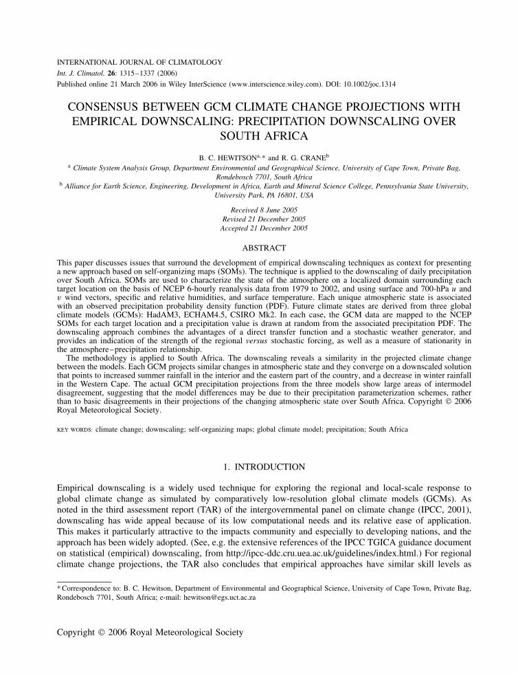
To explore the degree of local stochastic versus synoptic forcing, Figure 4 picks one target location in thesummer convective rainfall region (26 °S; 28 °E) and shows the median time series of monthly mean totalsover 6 years, along with the one standard deviation envelope of the 150 realizations of downscaling conductedfor this target. The figure shows how the downscaling captures the interannual variability, and indicates howwide the stochastic envelope is, demonstrating how the degree of stochastic control is seasonally dependant.In this case, we see that for this summer rainfall region, as one might expect, the stochastic componentincreases for summer months when rainfall is a product of convective processes.

5.2. Assessment of GCM circulation

Before examining the downscaled climate change from the GCMs, it is valuable to first consider thechanges in atmospheric circulation projected by the GCMs, and how this relates to the issue of stationarity.Figure 5 takes a downscaling target location – one in the summer convective regime on the interior plateau,and explores the frequency attributes of the associated 3 × 3 cell atmospheric predictor window.

Figure 5 shows the frequency of days mapped to each of the SOM nodes for the NCEP data, by contouringthe frequency across the 9 × 11 node array. Each node has an associated reference vector, representing thegeneralized atmospheric state. These generalized atmospheric states could be plotted as nine figures (one for



200

300

300

400 500

500

500

500

400

300600

600

500

400

400

600

700

600

900

500

600

200

200

400

400200

200100

700

300

800

700800

21S

22S

23S

24S

25S

26S

27S

28S

29S

30S

31S

32S

33S

34S

35S16E 18E 20E 22E 24E 26E 28E 30E 32E

Observed: Annual total (mm)

100

300

300

300

300

300

100200

400

400 400

300

300 600

400

500

200

500

500600

600

900

500

600700

500

600700

7001000

400

100

100

100

100

100

200 200

200

200

200

900

400700800

800

800600

800

700

500

21S

22S

23S

24S

25S

26S

27S

28S

29S

30S

31S

32S

33S

34S

35S16E 18E 20E 22E 24E 26E 28E 30E 32E

Downscaled: Annual mean total (mm)

(a)

(b)

Figure 1. Mean annual total precipitation (mm). Observed mean precipitation totals (a) from gridded station precipitation (Hewitsonand Crane, 2005), and empirically downscaled precipitation (b) from NCEP atmospheric circulation fields, for the period 1979–1999



2

22

4

4

4

2

6

8

10

4

2

22

2

2

2

2

6

4

4

4

4

4

48 8 6

4

2

4

8

8

8

6

4

4

4

6

8

2 2

6

6

8 864

2

2

6

4

4

4

4

4

10 10

10

10

10

10

12

1214 16 16

1818

20

20

14 2412

22

1212 18

18

16

16

14

10

16

1212

12

14

14

6

8

8

8

8 86

4

6

6

1416

20 18

18

18

48

8

6

6

6

22

2

24

4 2

2

2

2

2

24

2

486

4

2

410

68 8

8

86

6

44

4

6

10

12

16

14

8

1612

1414

16

20

1214

20

1012

10

10

10

14 12 10

12

10

12

10

12

121214

10

1618

12

16

14

14

14

1210

10

101416

6

21S

22S

23S

24S

26S

25S

27S

28S

29S

30S

31S

32S

33S

34S

35S16E 18E 20E 22E 24E 26E 28E 30E 32E

Observed: Average raindays / month (DJF)

21S

22S

23S

24S

26S

25S

27S

28S

29S

30S

31S

32S

33S

34S

35S16E 18E 20E 22E 24E 26E 28E 30E 32E

Downscaled: Average raindays / month (DJF) Downscaled: Average raindays / month (JJA)21S

22S

23S

24S

26S

25S

27S

28S

29S

30S

31S

32S

33S

34S

35S16E 18E 20E 22E 24E 26E 28E 30E 32E

21S

22S

23S

24S

26S

25S

27S

28S

29S

30S

31S

32S

33S

34S

35S16E 18E 20E 22E 24E 26E 28E 30E 32E

Observed: Average raindays / month (JJA)

0

Figure 2. Mean number of rain days per month for summer (December, January, February (DJF) – left panels) and winter (June, July,August (JJA) – right panels) observed (top) and empirically downscaled (bottom), for the period 1979–1999

each variable), where each figure would consist of a matrix of 9 × 11 maps. To save space, these are notpresented here (see Hewitson and Crane, 2002, for an example of a SOM node mapping of synoptic pressurefields). The NCEP map shows the distribution of occurrence of atmospheric states, in effect a two-dimensionalhistogram. As is common with SOMs, the centers of high frequency are located near the edges and cornersof the map (Hewitson and Crane, 2002).

The remainder of Figure 5 shows, in each column, the results for each of three GCMs: the HadAM3, theECHAM4.5, and the CSIRO9 Mk2. Given that the GCMs are being mapped to an SOM already trained by theNCEP data, one could anticipate several possible outcomes. If the GCM data map to the SOM nodes with afrequency distribution very similar to the NCEP data, it would indicate that the GCM has the same synoptic-scale structure and temporal behavior as the observed climate. Alternatively, the GCM could map to the SOMwith a very different frequency distribution, indicating some differences in the temporal characteristics of the



25

25

25

2550 50

5025

25

25

75

0

100125

2575

75

75

75

25

25 2550

100100

200150

125 125

50100

100

175

12525

5050

150

125125

150

−20

−10

−10 −30

−15−20

−40−35

−45

−10

−5

−20–55

−20−30−50

−35

−40

−25

−5

−5

−5 −5−5−15

50

75 75

75

100

125

0

0

0

00

−10

−5

−5

−50

00 0

0

000

0

0

0

0

00 0 0

0 –5

0

25

75

25

25

25

50

100

0

100125

100175

−10

–45–40–35−30

−70−65−65−60 −45−30−25−25

−20−25−25

−15−5−30−25−20

–40–35−10

–60−55–50−45–40–35−30−15

−50−25

−25−20−20

−15

21S

22S

23S

24S

25S

26S

27S

28S

29S

30S

31S

32S

33S

34S

35S16E 18E 20E 22E 24E 26E 28E 30E 32E

21S

22S

23S

24S

25S

26S

27S

28S

29S

30S

31S

32S

33S

34S

35S16E 18E 20E 22E 24E 26E 28E 30E 32E

21S

22S

23S

24S

25S

26S

27S

28S

29S

30S

31S

32S

33S

34S

35S16E 18E 20E 22E 24E 26E 28E 30E 32E

21S

22S

23S

24S

25S

26S

27S

28S

29S

30S

31S

32S

33S

34S

35S16E 18E 20E 22E 24E 26E 28E 30E 32E

21S

22S

23S

24S

25S

26S

27S

28S

29S

30S

31S

32S

33S

34S

35S16E 18E 20E 22E 24E 26E 28E 30E 32E

21S

22S

23S

24S

25S

26S

27S

28S

29S

30S

31S

32S

33S

34S

35S16E 18E 20E 22E 24E 26E 28E 30E 32E

Full train: Dec−Jan−Feb (mm) Full train: Jun−Jul−Aug (mm)

Independant Test: Dec−Jan−Feb (mm) Independant Test: Jun−Jul−Aug (mm)

Full Train − Test: Jun−Jul−Aug (mm)Full Train − Test: Dec−Jan−Feb (mm)

50

Figure 3. Comparison of downscaled mean monthly precipitation (mm) for summer (DJF – left panels) and winter (JJA – right panels)over eight random years when using the full record from 1979 to 2002 to train the downscaling, or a partial record. The top panelsare the downscaled precipitation for the eight random years from the SOMs trained with the full record. The middle panels are thedownscaled precipitation for the 8 years when these years are excluded from the training of the SOMs. The lower panels show the

anomaly between the twoCopyright 2006 Royal Meteorological Society Int. J. Climatol. 26: 1315–1337 (2006)


250

200

150

100

50

0

Pre

cipi

tatio

n (m

m)

1 695 9 13 17 21 25 29 33 37 41 45 49 53 57 61 65

Months

Figure 4. Sample of 6 years of monthly precipitation (thick line), bounded by 1 standard deviation of the 150 downscaled series forthese years. The downscaled data are for a summer rainfall location. The graph demonstrates that the degree of stochastic variability

varies seasonally, yet the downscaled data captures the large scaled circulation forcing of both the intra- and interannual variability

circulation. If the frequencies clustered in one section of the map, it would indicate a substantial differencebetween the observed and modeled atmospheres, with a large portion of the model atmospheric states mostlikely lying outside of the SOM domain. Focusing on the top row of Figure 5 (the frequency distributionacross the nodes for the GCM control simulation of present-day climate) it is apparent that the GCMs havedistributions similar to that of NCEP, but with higher frequencies centered on fewer nodes – suggestingthat the modeled climate represents a reduced dimensionality and lower variability system compared to theobserved climate. Note, however, that the models generally occupy the same feature space as the observed(NCEP) climate. However, the models all show a preference for different atmospheric modes, revealing amode bias that varies between GCMs.

The second row of Figure 5 shows the frequency distribution of the simulated future climates, in generalshowing a similar distribution to the control runs. Nodes that had high frequency counts in the control runhave even higher counts in the future climate, and day-to-day variability is further reduced. The bottom rowof the figure shows the anomaly of frequency change. While the frequency distribution of daily circulationstates from the control run shows differences between models, and each model has different bias compared tothe NCEP frequency distribution, the models’ climate change circulation anomalies show marked similaritiesbetween GCMs. This suggests that while the models have unique bias, the dynamic response to anthropogenicgreenhouse gas forcing is comparable. Given that the precipitation fields from GCM climate change projectionsoften show marked disagreement between GCMs (see later), this commonality of dynamic circulation responsesuggests that the climate change signal can be coherent between models: that perhaps the parameterization ofdiagnostic variables such as precipitation is a significant contributor to the intermodel differences in projectionsof precipitation change. If this is the case, empirical downscaling as presented here potentially can expose amore robust climate change signal between multiple GCMs – given that it is based on the spatial nature ofthe dynamic circulation response.

Figure 6 expands on the examination of GCM circulation and explores more explicitly the issue ofstationarity. Each node reference vector represents a mean state for a subregion of the data space, as discussedearlier. When observations are mapped to a given node of the SOM, there is an error factor: a measure ofthe degree to which the node reference vector exactly represents the observation vector. As the data arestandardized, the values are standardized units, and represent the mean absolute error of the comparison ofdata vector with the reference vector, giving an indication of the variability of observations mapping to agiven node.

Plotted in Figure 6 is the mean error with which the NCEP atmospheric states map to each node. For themost part the error is consistent across the nodes, indicating the nodes effectively represent the span of the data


1328 B. C. HEWITSON AND R. G. CRANEC

SIR

O c

ontr

ol

CS

IRO

Fut

ure

EC

HA

M F

utur

e

EC

HA

M c

ontr

olH

adA

M c

ontr

olN

CE

P

Had

AM

Fut

ure

Had

AM

Fut

ure−

Con

trol

EC

HA

M F

utur

eC

SIR

O F

utur

e−C

ontr

ol

8 7 6 5 4 3 2 1 0

87

65

43

21

010

9

87

65

43

21

010

9

87

65

43

21

010

98

76

54

32

10

109

87

65

43

21

010

9

87

65

43

21

010

9

87

65

43

21

010

9

87

65

43

21

010

98

76

54

32

10

109

87

65

43

21

010

9

8 7 6 5 4 3 2 1 0 8 7 6 5 4 3 2 1 0

8 7 6 5 4 3 2 1 0 8 7 6 5 4 3 2 1 0 8 7 6 5 4 3 2 1 0

8 7 6 5 4 3 2 1 0

8 7 6 5 4 3 2 1 0

8 7 6 5 4 3 2 1 0 8 7 6 5 4 3 2 1 0

1.4

1.2 1

1

0.8

0.8

0.2

−0.2

−0.2

−0.2

−0.2

−0.2

−0.2

0.4

0.4

0.4

0.4

0.6

0.4

0.4

0.2

0.2

−0.4

−0.4

−0.4

−0.4

−0.4

−0.4

−0.4

1.4

1.4

1.4

1.4

2.4

1.2

1.2

1.2

1.2

2.2

1.2

11

1

0.6

0.6

−0.6

−0.6

−0.6

0.6

0.6

0.8

0.6

0.6

0.8

0.8

0.8

0.8

0.8

0.8

0.8

0.8

0.9

0.9

1 1

1.1

1

1

0.9

0.9

0.8

0.8

0.8

0.4

0.6

0.6

0.6

1.4

1.2

1

11

1

1

0

00

0−0

.2

0

1

1

1

Figu

re5.

Freq

uenc

ydi

stri

butio

nac

ross

the

SOM

node

sfo

rat

mos

pher

icci

rcul

atio

nce

nter

edon

26° S

and

28° E

.T

heto

pro

wsh

ows

the

freq

uenc

ypl

otfo

rci

rcul

atio

nfie

lds

inth

eN

CE

Pre

anal

ysis

data

,and

inth

eco

ntro

lpe

riod

sim

ulat

ion

data

ofth

eth

ree

GC

Ms.

The

mid

dle

row

show

sth

efr

eque

ncy

dist

ribu

tion

for

the

futu

recl

imat

eas

sim

ulat

edby

the

thre

eG

CM

s.T

helo

wes

tro

wsh

ows

the

freq

uenc

yan

omal

ybe

twee

nth

efu

ture

and

cont

rol

clim

ate

sim

ulat

ions

for

the

thre

eG

CM

s



87

65

43

21

010

98

76

54

32

10

109

87

65

43

21

010

98

76

54

32

10

109

87

65

43

21

010

98

76

54

32

10

109

87

65

43

21

010

9

87

65

43

21

010

98

76

54

32

10

109

87

65

43

21

010

9

8 7 6 5 4 3 2 1 0

8 7 6 5 4 3 2 1 0 8 7 6 5 4 3 2 1 0 8 7 6 5 4 3 2 1 0

8 7 6 5 4 3 2 1 0 8 7 6 5 4 3 2 1 0 8 7 6 5 4 3 2 1 0

8 7 6 5 4 3 2 1 0 8 7 6 5 4 3 2 1 0 8 7 6 5 4 3 2 1 0

NC

EP

nod

e er

ror

Had

AM

con

trol

nod

e er

ror

Had

AM

Fut

ure

node

err

orE

CH

AM

Fut

ure

node

err

orC

SIR

O F

utur

e no

de e

rror

EC

HA

M F

utur

e−C

ontro

l nod

e er

ror (

%)

CS

IRO

Fut

ure−

Con

trol n

ode

erro

r (%

)H

adA

M F

utur

e−C

ontro

l nod

e er

ror (

%)

EC

HA

M c

ontr

ol n

ode

erro

rC

SIR

O c

ontr

ol n

ode

erro

r

4.5

4.5

4.5

5.5

4.5

4.5

4.5

5.5

5.5

5.5

5.5

5.5

6.5 7

6

5.5

5.5

5.5

5.5

5.5

6.5

6.5

5 5

5

5

5

5

0 0

50 55 60

20

15

30 303555 50 4045 35

5

5

56

6

6

6

44 4

4

6

6

Figu

re6.

Mea

nno

deer

ror

ofda

ysm

appi

ngto

the

SOM

node

sfo

rat

mos

pher

icci

rcul

atio

nce

nter

edon

26° S

and

28° E

.The

top

row

show

sth

eno

deer

ror

for

circ

ulat

ion

field

sin

the

NC

EP

rean

alys

isda

ta,

and

inth

eco

ntro

lpe

riod

sim

ulat

ion

data

ofth

eth

ree

GC

Ms.

The

mid

dle

row

show

sth

eno

deer

rors

for

the

futu

recl

imat

eas

sim

ulat

edby

the

thre

eG

CM

sw

hen

map

ped

toth

eSO

M.

The

low

est

row

show

sth

epe

rcen

tch

ange

inth

eno

deer

ror

betw

een

the

futu

rean

dco

ntro

lcl

imat

esi

mul

atio

nsfo

rth

eth

ree

GC

Ms,

whe

reth

em

agni

tude

ofth

ech

ange

isin

dica

tive

ofth

ede

gree

tow

hich

futu

resy

nopt

icst

ates

exce

edth

een

velo

peof

the

cont

rol

clim

ate



across the n-dimensional data space. The remainder of panels in the top row of Figure 6 indicates the nodeerror for the GCM control simulations, with the second row showing the node error from the simulationsof the future climate. The mapping of the GCM data to the nodes show increased error over the NCEPdata – indicating that the GCMs simulate circulation states that, although representing similar atmosphericstates to the NCEP data, have some degree of disparity and bias. It is possible to investigate this furtherby examining the atmospheric states of the nodes in which the GCM data are most deviant from the NCEPdefined states, and so understand which dynamic processes in the model are less well simulated. However,such analysis is beyond the scope of this paper.

The lowest row of Figure 6 is the change in the error factor between the GCM control and future simulationdata. Two attributes are of note here: first that, as in Figure 5, the model-simulated change between the controland future climate again shows remarkable agreement between GCMs. This supports the earlier suggestionthat there is a robust change signal between GCMs in terms of the circulation dynamics. More relevantwith reference to stationarity, is the degree to which the error of the future climate mapping to the SOMnodes exceeds the error of the control run data. It is clear that the future simulation data show an increasein the mapping error, indicating a measure of non-stationarity in the circulation. A way to consider thisis to understand that the control simulation data define an envelope of the climate. The future simulationsimilarly has a climate envelope; however, there is a non-perfect overlap of the two climate envelopes – theclimate envelope has shifted. The anomaly node error plots of Figure 6 are thus a measure of the GCM’sdata stationarity. For the most part, the non-stationarity component of the future climate is relatively small;most nodes have changes in mapping error in the range of 0–20%. A few nodes show moderate growth innon-stationarity, with some nodes, in particular with the ECHAM model, having a change of up to 60%.

On one level, the stationarity issue is a potential problem, especially if one were using a transfer functionbetween the circulation and the precipitation based on, for example, some form of linear or nonlinearregression. However, in the case of the SOM downscaling, the procedure is inherently conservative. If afuture climate data sample fell outside of the envelope of climate defined by the data used to train the SOM,the data sample would then be mapped back to the node that is closest within the n-dimensional data space.By selecting rainfall amounts from these nodes, we have a conservative estimate of the future climate responseand, at worst, we underestimate the change.

In light of this conservative attribute of the downscaling in the presence of non-stationarity, the procedureprovides a robust means to downscale the climate change signal. For example, dominant anticyclonic systemsover a region may increase beyond the intensity of present-day climate. However, in such a situation thedownscaling would still reflect a local climate response of a dominant anticyclonic system, only for that ofa less intense system.

5.3. Downscaled climate change

The downscaled precipitation needs to be viewed in the light of what the GCM parameterized precipitationindicates. Figure 7 shows typical GCM climate change anomalies for precipitation, contoured in terms ofthe change in mean annual precipitation – the magnitudes of the anomaly reflect a 10–15% change. Notableis the disagreement between the three GCMs; CSIRO-Mk2 shows a decrease over effectively the wholedomain while the ECHAM4.5 and HadAM3 show drying in most of the domain, with increases over theeastern portion, although disagreeing in the spatial extent and magnitude of the increase. Note, these GCMprecipitation fields are from the IPCC DDC (Data distribution center. See http://ipcc-ddc.cru.uea.ac.uk/)archive of monthly mean values for these models, as the daily precipitation data for the models were notavailable for this study. Nonetheless, the results are reflective of the typical GCM consensus (or lack thereof).

One way of using the GCM precipitation information in Figure 7 would be to present an average of thethree maps, or to present the differences between the maps as a measure of uncertainty – to provide high andlow bounds for a climate scenario. Both approaches are problematic. This is not simply a case of differentestimates of the magnitude of the change or a slight phase shift or offset in the location of some controllingfeature (such as storm tracks, etc.). These are not three variations of a similar climate response, and averagingthe three makes very little sense. If the models are simulating precipitation accurately, these could represent



16E 18E 20E 22E 24E 26E 28E 30E 32E 34E

22S

23S

24S

25S

26S

27S

28S

29S

30S

31S

32S

33S

34S

35S

CSIRO A2 Mean annual anomaly (mm)

−300−325

−50−25

0

−25

−75

0

−275

−50

75

−300−275

−200−175−150−125

−75

−250

−100

−225

16E 18E 20E 22E 24E 26E 28E 30E 32E 34E

22S

23S

24S

25S

26S

27S

28S

29S

30S

31S

32S

−25

33S

34S

35S

−100

−50

100

125150

75

50

025−25

0

−50

−75

−100−50

175

175

−100

1

ECHAM A2 Mean annual anomaly (mm)

(a)

(b)

Figure 7. Projected climate change anomaly in mean annual precipitation from three GCMs

three equally possible responses to the same forcing, and the differences could be regarded as a measureof uncertainty in the climate system. However, if the differences are due to differences in the precipitationparameterization schemes and their interaction with the model dynamics (or the model topography, landsurface climatology, etc.), then the three maps represent more a measure of uncertainty in our ability toeffectively simulate the climate system over this region. Either way, the differences in sign, spatial patterns,and anomaly gradients across the region indicate that the GCM precipitation fields provide little informationthat would be beneficial for impacts assessment.



16E 18E 20E 22E 24E 26E 28E 30E 32E 34E

22S

23S

24S

25S

26S25

5027S

28S

29S 25

30S 0

31S

32S

33S

34S

35S

HadCM3 A2 Mean annual anomaly (mm)

−200−175−150

−50

−25−125

−25

−100

−50−75

5050

75

−25

−50

−50

−150

−100−75−50

175−150−75

025

325−300−27−230−2252−175−125−100

−150

(c)

Figure 7. (Continued)

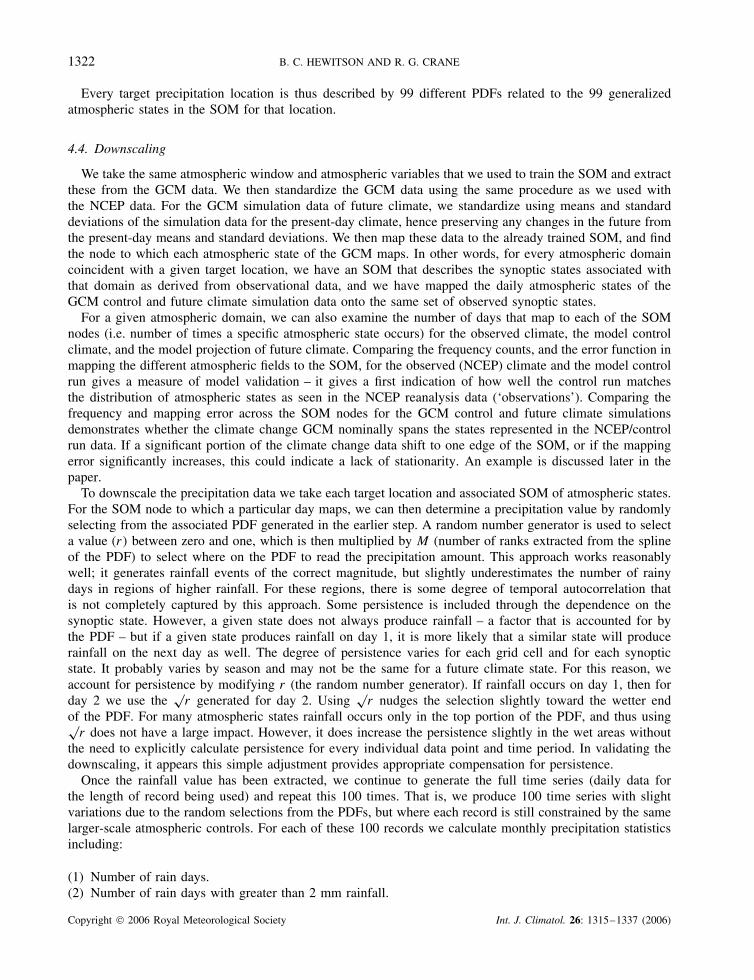
The downscaling results present a very different picture. Figure 8 shows the climate change anomaly fromdifferencing the downscaled control and future daily atmospheric data of the three GCMs. Two facts are ofimmediate note: the downscaling provides regional detail that is consistent with the actual spatial gradientsover the region, and the pattern agreements of positive and negative changes are remarkably consistentacross the three GCMs. This general agreement in the direction and spatial distribution of the changes is inmarked contrast to Figure 7. The most likely explanation is that all the models capture the larger-scale forcingreasonably well, and all of them project similar changes in atmospheric state for this region. Consequently,the downscaled results show similar distributions, which would also suggest that much of the difference inFigure 7 is due to differences in the way the models derive their precipitation values, rather than disagreementsover their projection of future atmospheric circulation. This same consistency is seen in Figure 9, which showschanges in the number of rain days, and Figure 10, which shows changes in the number of days with a rainfallover 20 mm. The ECHAM4.5 forced downscaling shows a far stronger downscaled response than the othertwo models, and reflects the concentration of the circulation change toward a (wet) subset of synoptic modesas shown in Figure 5.

Two localized regions of disagreement are: first, the mild winter increase in precipitation over the southwestcorner of South Africa by the HadAM3 model, in contrast to the drying in the other two models, and second,the mild increase over the northern border in summer shown by the ECHAM4.5 model, whereas the othertwo models indicate drying. However, in the latter case, the ECHAM4.5 model already appears to be far toowet in summer, and this may result in the model atmospheric states over the northern border not reflectingthe drying as seen in the other two models.

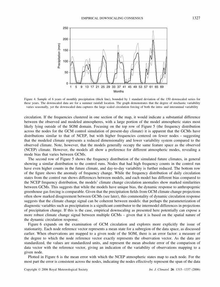
As noted earlier, since the downscaling generates daily data, it is possible to calculate a number of relevantstatistics about the attributes of the daily precipitation. In Figures 9 and 10 we show the climate changeanomaly in the number of rain days with precipitation greater than 2 mm and greater than 20 mm (heavyrainfall days). These are parameters of particular significance for hydrology and water resources, as well asagriculture. At the same time, this is a difficult parameter to estimate from GCMs, as the GCM grid cells tendto precipitate on most days, being a large area average parameter. The downscaled rain day anomalies trackthe spatial changes in rainfall totals to a fair degree, but not completely, in some cases showing a decreasein rain days where totals increase, or vice versa, and indicating that there are changes in intensity as well.



Jun−

Jul−

Aug

: H

adA

M a

nom

aly

(mm

)

Dec

−Jan

−Feb

: H

adA

M a

nom

aly

(mm

)D

ec−J

an−F

eb :

EC

HA

M a

nom

aly

(mm

)D

ec−J

an−F

eb :

CS

IRO

ano

mal

y (m

m)

Jun−

Jul−

Aug

: E

CH

AM

ano

mal

y (m

m)

Jun−

Jul−

Aug

: C

SIR

O a

nom

aly

(mm

)21

S22

S23

S24

S25

S26

S27

S28

S29

S30

S31

S32

S33

S34

S35

S

21S

22S

23S

24S

25S

26S

27S

28S

29S

30S

31S

32S

33S

34S

35S

21S

22S

23S

24S

25S

26S

27S

28S

29S

30S

31S

32S

33S

34S

35S

21S

22S

23S

24S

25S

26S

27S

28S

29S

30S

31S

32S

33S

34S

35S

21S

22S

23S

24S

25S

26S

27S

28S

29S

30S

31S

32S

33S

34S

35S

21S

22S

23S

24S

25S

26S

27S

28S

29S

30S

31S

32S

33S

34S

35S

16E

18E

20E

22E

24E

26E

28E

30E

32E

16E

18E

20E

22E

24E

26E

28E

30E

32E

16E

18E

20E

22E

24E

26E

28E

30E

32E

16E

18E

20E

22E

24E

26E

28E

30E

32E

16E

18E

20E

22E

24E

26E

28E

30E

32E

16E

18E

20E

22E

24E

26E

28E

30E

32E

5

5

5

5

5

5

5 5

10

10

10

15

15

10

1010

10

−15

0

0

0

0

0

0

010

1020

515

2515

30

5

5

1525

25

40

40

75

20

20 15

15

15

15

35 35

50

60 60

10

10

45

45

45

55

5 5

5

5

8030

25

25 3050

65

5560

65 70

10

10

10

20

20

55

5

55

5

5

5

5

25

15

1515

0

0

0758085

85 90

70

Figu

re8.

Proj

ecte

dcl

imat

ech

ange

anom

aly

ofm

ean

mon

thly

prec

ipita

tion

(mm

)fo

rsu

mm

er(D

JF)

and

win

ter

(JJA

),de

rive

dfr

omth

edo

wns

cale

dda

ilypr

ecip

itatio

nfr

omea

chof

the

thre

eG

CM

s



21S

22S

23S

24S

25S

26S

27S

28S

29S

30S

31S

32S

33S

34S

35S

16E

18E

20E

22E

24E

26E

28E

30E

32E

Jun−

Jul−

Aug

: H

adA

M a

nom

aly

0.5

0.5

0.5

1.5

1

1

1

0

21S

22S

23S

24S

25S

26S

27S

28S

29S

30S

31S

32S

33S

34S

35S

16E

18E

20E

22E

24E

26E

28E

30E

32E

Jun−

Jul−

Aug

: E

CH

AM

ano

mal

y

0.5

0.5

0.5

1.51.5

2

2

1

11

−0.5

2.5

21S

22S

23S

24S

25S

26S

27S

28S

29S

30S

31S

32S

33S

34S

35S

16E

18E

20E

22E

24E

26E

28E

30E

32E

Jun−

Jul−

Aug

: C

SIR

O a

nom

aly

0.5

0.5

0.5

1.5

1.5

1.5

1.5

2

2

2

1

1

1

2.5

2.5

2.5

2.5

3

3

0

21S

22S

23S

24S

25S

26S

27S

28S

29S

30S

31S

32S

33S

34S

35S

16E

18E

20E

22E

24E

26E

28E

30E

32E

Dec

−Jan

−Feb

: C

SIR

O a

nom

aly

0.5

0.5

0.5

0.5

1.5

1.5

1.5

2

2

1

11

1 1

0

0

21S

22S

23S

24S

25S

26S

27S

28S

29S

30S

31S

32S

33S

34S

35S

16E

18E

20E

22E

24E

26E

28E

30E

32E

Dec

−Jan

−Feb

: E

CH

AM

ano

mal

y

0.5

0.5

1.5

1.5

1.5

1.5

2

2

2

1

1 11

3 3

3

3

3

3.5

3.5

3.53.5

2.5

2.5

2.5

4.5

4.5

4

4

4

3.5 4

21.5 2.5

21S

22S

23S

24S

25S

26S

27S

28S

29S

30S

31S

32S

33S

34S

35S

16E

18E

20E

22E

24E

26E

28E

30E

32E

Dec

−Jan

−Feb

: H

adA

M a

nom

aly

0.5

0.5

0.5

0.5

0.5

1.5

1.5

1.5

2.5 2

2

2

1

1

1

0

0 0

1.5

Figu

re9.

Proj

ecte

dcl

imat

ech

ange

anom

aly

ofth

em

ean

num

ber

ofra

inda

yspe

rm

onth

for

sum

mer

(DJF

)an

dw

inte

r(J

JA),

deri

ved

from

the

dow

nsca

led

daily

prec

ipita

tion

from

each

ofth

eth

ree

GC

Ms



21S

22S

23S

24S

25S

26S

27S

28S

29S

30S

31S

32S

33S

34S

35S

21S

22S

23S

24S

25S

26S

27S

28S

29S

30S

31S

32S

33S

34S

35S

21S

22S

23S

24S

25S

26S

27S

28S

29S

30S

31S

32S

33S

34S

35S

21S

22S

23S

24S

25S

26S

27S

28S

29S

30S

31S

32S

33S

34S

35S

21S

22S

23S

24S

25S

26S

27S

28S

29S

30S

31S

32S

33S

34S

35S

21S

22S

23S

24S

25S

26S

27S

28S

29S

30S

31S

32S

33S

34S

35S

Jun−

Jul−

Aug

: H

adA

M a

nom

aly

Jun−

Jul−

Aug

: E

CH

AM

ano

mal

yJu

n−Ju

l−A

ug :

CS

IRO

ano

mal

y

Dec

−Jan

−Feb

: C

SIR

O a

nom

aly

Dec

−Jan

−Feb

: E

CH

AM

ano

mal

yD

ec−J

an−F

eb :

Had

AM

ano

mal

y

0

0

16E

18E

20E

22E

24E

26E

28E

30E

32E

16E

18E

20E

22E

24E

26E

28E

30E

32E

16E

18E

20E

22E

24E

26E

28E

30E

32E

16E

18E

20E

22E

24E

26E

28E

30E

32E

16E

18E

20E

22E

24E

26E

28E

30E

32E

16E

18E

20E

22E

24E

26E

28E

30E

32E

0

0

0

0

0

0

0

00

0

0.3

0

0

000

0

0

00.

1

0.1

0.1

0.4 0.

4

−0.1

−0.1

0.2

0

0

0000

0

0.3

0.2

0.2

0.1

−0.1

0.1

00.

3

0.1

0.4

0.4

0.4

0.2

0 0.1

0.3

0

0.2

0.2

0.2

0.3

0.9

0.50.4

0.3

0.3 0.

1

0.1

0.8

0.5

1.1

1.2

1

0.40.6

0.6

0

0

0

0.7

0.7

0.6 1

.6

1.3

1.4 1.

41.

51.

61.

7

0.4

0.5

0.7

0.8

Figu

re10

.Pr

ojec

ted

clim

ate

chan

gean

omal

yof

heav

yra

infa

llev

ents

(rai

nda

ys>

20m

m)

per

mon

thfo

rsu

mm

er(D

JF)

and

win

ter

(JJA

),de

rive

dfr

omth

edo

wns

cale

dda

ilypr

ecip

itatio

nfr

omea

chof

the

thre

eG

CM

s



6. SUMMARY AND DISCUSSION

The development of regional climate change scenarios has been subject to debate, with the outcomes dependanton the GCM employed, the downscaling method used, and the assumptions involved. With the improvementin GCM skill, and the convergence in the circulation response to greenhouse gas forcing between GCMs, theopportunity exists to develop regional-scale scenarios of future change that are inherently consistent with theGCM forcing. The methodology presented here offers an inexpensive solution that may be quickly employedwith a broad range of GCM outputs, and one that is inherently conservative in the presence of non-stationarityin the climate system. The downscaled solutions for South Africa show notable coherency when forced byseveral different GCMs; the magnitudes of projected change differ, but the spatial pattern of the change islargely in agreement. The results indicate that South Africa will experience increased summer rainfall overthe convective region of the central and eastern plateau and the Drakensberg Mountains. The Western Capewill see little change, with some slight drying in summer and a slight decrease in wintertime frontal rainfall.

Questions remain around the probability of occurrence of any one emission scenario over another, and therelative value of the empirically downscaled projection versus that which may be derived from RCMs. Thefirst question is complex and, with current resources and data availability, is perhaps best approached throughdownscaling a range of GCM simulations forced with different, yet defensible, scenarios of future greenhousegas emissions. In this respect, empirical downscaling is particularly advantageous in terms of computationalefficiency. However, while the empirical techniques give a first-order response to the regional climate changethat is physically consistent with the circulation, they are not capable of incorporating local-scale feedbacks.RCMs, on the other hand, are able to accommodate such feedbacks, but it is arguable whether this providesany greater confidence in the downscaled solution, given the significant sensitivity of the RCM to choice ofparameterization schemes and physics packages. The selection of an empirical or modeling approach is likelyto be determined by the resources available and the specific study objectives. The present results point to thepotential for empirical techniques to demonstrate the convergence of different climate change projections frommultiple GCMs. At the same time, they present an economical way of assessing a range of climate changescenarios: results that could be extremely useful from the policy and planning perspective. Numerical RCMs,however, are essential for assessing the potential impacts of multiple forcing factors (e.g. global climate andregional land use change).

In conclusion, it would appear that spatially cohesive projections of regional climate change are possible,where the changes are consistent with the GCM forcing, coherent in pattern across different GCMs, anddefensible in terms of our understanding of the physical processes underpinning the change. The methodologyimplemented here is robust, conservative against stationarity, and readily implemented across multiple GCMswith minimal computation requirement.

REFERENCES

AchutaRao K, Sperber KR. 2002. Simulation of the El Nino Southern oscillation: Results from the coupled model intercomparisonproject. Climate Dynamics 19: 191–209.

Ambroise C, Seze G, Badran F, Thiria S. 2000. Hierarchical clustering of self-organizing maps for cloud classification. Neurocomputing30: 47–52.

Buishand TA, Shabalova MV, Brandsma T. 2004. On the choice of the temporal aggregation level for statistical downscaling ofprecipitation. Journal of Climate 17(9): 1816–1827.

Cavazos T. 1999. Large-scale circulation anomalies conducive to extreme events and simulation of daily precipitation in northeasternMexico and southeastern Texas. Journal of Climate 12: 1506–1523.

Cavazos T. 2000. Using self-organizing maps to investigate extreme events: An application to wintertime precipitation in the Balkans.Journal of Climate 13: 1718–1732.

Cavazos T, Hewitson BC. 2005. Performance of NCEP variables in statistical downscaling of daily precipitation. Climate Research 28:95–107.

Christensen JH, et al. 2005. Evaluation of the performance and utility of regional climate models in climate change research: Reducinguncertainties in climate change projections–the PRUDENCE approach. Climatic Change [In Press].

Covey C, AchutaRao KM, Cubasch U, Jones P, Lambert SJ, Mann ME, Phillips TJ, Taylor KE. 2003. An overview of results from thecoupled model intercomparison project. Global and Planetary Change 37: 103–133.

Crane RG, Hewitson BC. 1998. CO2 precipitation changes for the Susquehanna basin: Downscaling from the GENESIS generalcirculation model. International Journal of Climatology 18: 65–76.

Crane RG, Hewitson BC. 2003. Clustering and upscaling of station precipitation records to regional patterns using self-organizing maps(SOMs). Climate Research 25: 95–107.



Gao XJ, Luo Y, Lin WT, Zhao ZC, Giorgi F. 2003. Simulation of effects of landuse change on climate in China by a regional climatemodel. Advances in Atmospheric Sciences 20: 583–592.

Hewitson BC. 2003. Developing perturbations for climate change impact assessment. EOS 84: 337–348.Hewitson BC, Crane RG. 1996. Climate downscaling techniques and applications. Climate Research 7: 85–95.Hewitson BC, Crane RG. 2002. Self organizing maps: Applications to synoptic climatology. Climate Research 22: 13–26.Hewitson BC, Crane RG. 2005. Gridded area-averaged daily precipitation via conditional interpolation. Journal of Climate 18: 41–57.Hudson DA, 1998. Antarctic sea ice extent, Southern Hemisphere circulation and South African rainfall, PhD Thesis, University of

Cape Town: South Africa.IPCC (Intergovernmental Panel on Climate Change). Houghton JJ, Ding Y, Griggs DJ, Noguer M, van der Linden PJ, Dai X, Maskell K,

Johnson CA (eds). 2001. IPCC Working Group I, Cambridge University Press: Cambridge, p. 881.Kohonen T. 1989. Self-Organization and Associative Memory, 3rd edn. Springer-Verlag: Heidelberg.Kohonen T. 1990. The self-organizing map. Proceedings of the IEEE 78: 1464–1480.Kohonen T. 1991. Self-organizing maps: optimization approaches. In Proceedings of the International Conference on Artificial Neural

Networks , Espoo, Finland, June 1991, 981–990.Kohonen T. 1995. Self-Organizing Maps. Springer-Verlag: Heidelberg.Lambert SJ, Boer GJ. 2001. CMIP1 evaluation and intercomparison of coupled climate models. Climate Dynamics 17: 83–106.Landman W, Mason S. 1999. Change in the association between Indian Ocean sea-surface temperatures and summer rainfall over South

Africa and Namibia. International Journal of Climatology 19(13): 1477–1492.Malmgren BA, Winter A. 1999. Climate zonation in Puerto Rico based on principal components analysis and an artificial neural network.

Journal of Climate 12: 977–985.Ni F, Cavazos T, Hughes MK, Comrie AC, Funkhouser G. 2002. Cool season precipitation in the Southwestern United States since AD

1000: Comparison of linear and nonlinear techniques for reconstruction. International Journal of Climatology 22(13): 1645–1662.Rautenbach C, Smith I. 2001. Teleconnections between global sea-surface temperatures and the interannual variability of observed and

model simulated rainfall over southern Africa. Journal of Hydrology 254(1–4): 1–15.Sewell R, Landman W. 2001. Indo-Pacific relationships in terms of sea-surface temperature variations. International Journal of

Climatology 21(12): 1515–1528.Tennant W. 2003. An assessment of intraseasonal variability from 13-yr GCM simulations. Monthly Weather Review 131(9): 1975–1991.Tennant W. 2004. Considerations when using pre-1979 NCEP/NCAR reanalyses in the southern hemisphere. Geophysical Research

Letters 31: L11112, DOI:10.1029/2004GL019751.Taylor CM, Lambin EF, Stephane N, Harding RJ, Essery RJH. 2002. The influence of land use change on climate in the Sahel. Journal

of Climate 15: 3615–3629.Wilby RL, Charles SP, Zorita E, Timbal B, Whetton P, Mearns LO. 2004. Guidelines for Use of Climate Scenarios Developed from

Statistical Downscaling Methods. IPCC Task Group on Data and Scenario Support for Impact and Climate Analysis (TGICA):http://ipcc-ddc.cru.uea.ac.uk/guidelines/index.html.

Wilby RL, Wigley TML, Conway D, Jones PD, Hewitson BC, Main J, Wilks DS. 1998. Statistical downscaling of general circulationmodel output: A comparison of methods. Water Resources Research 34: 2995–3008.


consensus between gcm climate change projections with empirical downscaling: precipitation...

Documents