connectionist learning procedures - university of …hinton/absps/clp.pdf · artificial...

ARTIFICIAL INTELLIGENCE 185

Connectionist Learning Procedures

Geoffrey E. Hinton C o m p u t e r Sc ience D e p a r t m e n t , Univers i ty o f T o r o n t o ,

10 K i n g ' s Col lege R o a d , T o r o n t o , Ontar io , Canada M 5 S 1 A 4

ABSTRACT

A major goal of research on networks of neuron-like processing units is to discover efficient learning procedures that allow these networks to construct complex internal representations of their environment. The learning procedures must be capable of modifying the connection strengths in such a way that internal units which are not part of the input or output come to represent important features of the task domain. Several interesting gradient-descent procedures have recently been discovered. Each connection computes the derivative, with respect to the connection strength, of a global measure of the error in the performance of the network. The strength is then adjusted in the direction that decreases the error. These relatively simple, gradient-descent learning procedures work well for small tasks and the new challenge is to find ways of improving their convergence rate and their generalization abilities so that they can be applied to larger, more realistic tasks.

1. Introduction

Recent technological advances in VLSI and computer aided design mean that it is now much easier to build massively parallel machines. This has contributed to a new wave of interest in models of computation that are inspired by neural nets rather than the formal manipulation of symbolic expressions. To understand human abilities like perceptual interpretation, content-addressable memory, commonsense reasoning, and learning it may be necessary to understand how computation is organized in systems like the brain which consist of massive numbers of richly interconnected but rather slow processing elements.

This paper focuses on the question of how internal representations can be learned in "connectionist" networks. These are a recent subclass of neural net models that emphasize computational power rather than biological fidelity. They grew out of work on early visual processing and associative memories [28, 40, 79]. The paper starts by reviewing the main research issues for connectionist models and then describes some of the earlier work on learning procedures for associative memories and simple pattern recognition devices. These learning procedures cannot generate internal representations: They are

Artificial Intelligence 40 (1989) 185-234 0004-3702/89/$3.50 ~) 1989, Elsevier Science Publishers B.V. (North-Holland)

186 G . E . H I N T O N

limited to forming simple associations between representations that are specified externally. Recent research has led to a variety of more powerful connectionist learning procedures that can discover good internal representations and most of the paper is devoted to a survey of these procedures.

2. Connectionist Models

Connectionist models typically consist of many simple, neuron-like processing elements called "units" that interact using weighted connections. Each unit has a "state" or "activity level" that is determined by the input received from other units in the network. There are many possible variations within this general framework. One common, simplifying assumption is that the combined effects of the rest of the network on the jth unit are mediated by a single scalar quantity, xj. The quantity, which is called the "total input" of unit j, is usually taken to be a linear function of the activity levels of the units that provide input to j:

xj = -Oj + ~ yiwji, (1) i

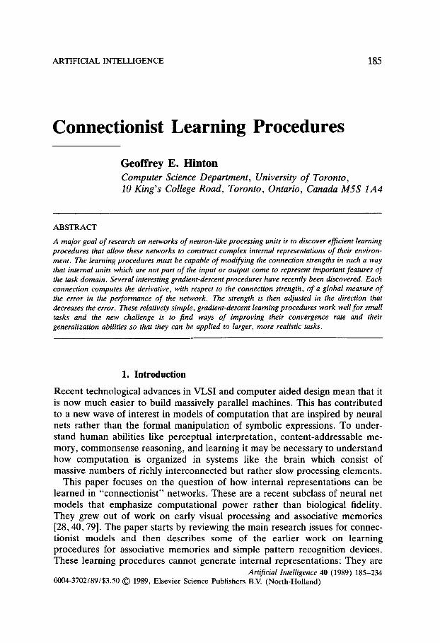
where Yi is the state of the ith unit, wji is the weight on the connection from the ith to the jth unit and 0j is the threshold of the jth unit. The threshold term can be eliminated by giving every unit an extra input connection whose activity level is fixed at 1. The weight on this special connection is the negative of the threshold. It is called the "bias" and it can be learned in just the same way as the other weights. This method of implementing thresholds will generally be assumed in the rest of this paper. An external input vector can be supplied to the network by clamping the states of some units or by adding an input term, lj, that contributes to the total input of some of the units. The state of a unit is typically defined to be a nonlinear function of its total input. For units with discrete states, this function typically has value 1 if the total input is positive and value 0 (or -1 ) otherwise. For units with continuous states one typical nonlinear input-output function is the logistic function (shown in Fig. 1):

1 YJ - 1 + e-Xj " (2)

All the long-term knowledge in a connectionist network is encoded by where the connections are or by their weights, so learning consists of changing the weights or adding or removing connections. The short-term knowledge of the network is normally encoded by the states of the units, but some models also have fast-changing temporary weights or thresholds that can be used to encode temporary contexts or bindings [44, 96].

CONNECTIONIST LEARNING PROCEDURES 187

1.0

~--->

Fig. 1. The logistic input-output function defined by equation (2). It is a smoothed version of a step function.

There are two main reasons for investigating connectionist networks. First, these networks resemble the brain much more closely than conventional computers. Even though there are many detailed differences between connectionist units and real neurons, a deeper understanding of the computational properties of connectionist networks may reveal principles that apply to a whole class of devices of this kind, including the brain. Second, connectionist networks are massively parallel, so any computations that can be performed efficiently with these networks can make good use of parallel hardware.

3. Connectionist Research Issues

There are three main areas of research on connectionist networks: Search, representation, and learning. This paper focuses on learning, but a very brief introduction to search and representation is necessary in order to understand what learning is intended to produce.

3.1. Search

The task of interpreting the perceptual input, or constructing a plan, or accessing an item in memory from a partial description can be viewed as a constraint satisfaction search in which information about the current case (i.e. the perceptual input or the partial description) must be combined with knowledge of the domain to produce a solution that fits both these sources of constraint as well as possible [12]. If each unit represents a piece of a possible solution, the weights on the connections between units can encode the degree of consistency between various pieces. In interpreting an image, for example, a unit might stand for a piece of surface at a particular depth and surface orientation. Knowledge that surfaces usually vary smoothly in depth and orientation can be encoded by using positive weights between units that represent nearby pieces of surface at similar depths and similar surface

188 G.E. HINTON

orientations, and negative weights between nearby pieces of surface at very different depths or orientations. The network can perform a search for the most plausible interpretation of the input by iteratively updating the states of the units until they reach a stable state in which the pieces of the solution fit well with each other and with the input. Any one constraint can typically be overridden by combinations of other constraints and this makes the search procedure robust in the presence of noisy data, noisy hardware, or minor inconsistencies in the knowledge.

There are, of course, many complexities: Under what conditions will the network settle to a stable solution? Will this solution be the optimal one? How long will it take to settle? What is the precise relationship between weights and probabilities? These issues are examined in detail by Hummel and Zucker [52], Hinton and Sejnowski [45], Geman and Geman [31], Hopfield and Tank [51] and Marroquin [65].

3.2. Representation

For tasks like low-level vision, it is usually fairly simple to decide how to use the units to represent the important features of the task domain. Even so, there are some important choices about whether to represent a physical quantity (like the depth at a point in the image) by the state of a single continuous unit, or by the activities in a set of units each of which indicates its confidence that the depth lies within a certain interval [10].

The issues become much more complicated when we consider how a complex, articulated structure like a plan or the meaning of a sentence might be represented in a network of simple units. Some preliminary work has been done by Minsky [67] and Hinton [37] on the representation of inheritance hierarchies and the representation of frame-like structures in which a whole object is composed of a number of parts each of which plays a different role within the whole. A recurring issue is the distinction between local and distributed representations. In a local representation, each concept is represented by a single unit [13, 27]. In a distributed representation, the kinds of concepts that we have words for are represented by patterns of activity distributed over many units, and each unit takes part in many such patterns [42]. Distributed representations are usually more efficient than local ones in addition to being more damage-resistant. Also, if the distributed representation allows the weights to capture important underlying regularities in the task domain, it can lead to much better generalization than a local representation [78, 80]. However, distributed representations can make it difficult to represent several different things at the same time and so to use them effectively for representing structures that have many parts playing different roles it may be necessary to have a separate group of units for each role so that the assignment of a filler to a role is represented by a distributed pattern of activity over a group of "role-specific" units.


Much confusion has been caused by the failure to realize that the words "local" and "distributed" refer to the relationship between the terms of some descriptive language and a connectionist implementation. If an entity that is described by a single term in the language is represented by a pattern of activity over many units in the connectionist system, and if each of these units is involved in representing other entities, then the representation is distributed. But it is always possible to invent a new descriptive language such that, relative to this language, the very same connectionist system is using local representations.

3.3. Learning

In a network that uses local representations it may be feasible to set all the weights by hand because each weight typically corresponds to a meaningful relationship between entities in the domain. If, however, the network uses distributed representations it may be very hard to program by hand and so a learning procedure may be essential. Some learning procedures, like the perceptron convergence procedure [77], are only applicable if the desired states of all the units in the network are already specified. This makes the learning task relatively easy. Other, more recent, learning procedures operate in networks that contain "hidden" units [46] whose desired states are not specified (either directly or indirectly) by the input or the desired output of the network. This makes learning much harder because the learning procedure must (implicitly) decide what the hidden units should represent. The learning procedure is therefore constructing new representations and the results of learning can be viewed as a numerical solution to the problem of whether to use local or distributed representations.

Connectionist learning procedures can be divided into three broad classes: Supervised procedures which require a teacher to specify the desired output vector, reinforcement procedures which only require a single scalar evaluation of the output, and unsupervised procedures which construct internal models that capture regularities in their input vectors without receiving any additional information. As we shall see, there are often ways of converting one kind of learning procedure into another.

4. Associative Memories without Hidden Units

Several simple kinds of connectionist learning have been used extensively for storing knowledge in simple associative networks which consist of a set of input units that are directly connected to a set of output units. Since these networks do not contain any hidden units, the difficult problem of deciding what the hidden units should represent does not arise. The aim is simply to store a set of associations between input vectors and output vectors by modifying the weights on the connections. The representation of each association is typically distrib-

190 G.E. HINTON

uted over many connections and each connection is involved in storing many associations. This makes the network robust against minor physical damage and it also means that weights tend to capture regularities in the set of input-output pairings, so the network tends to generalize these regularities to new input vectors that it has not been trained on [6].

4.1. Linear associators

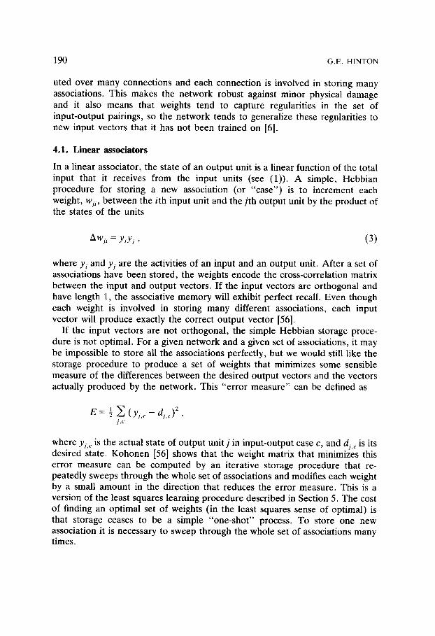
In a linear associator, the state of an output unit is a linear function of the total input that it receives from the input units (see (1)). A simple, Hebbian procedure for storing a new association (or "case") is to increment each weight, wji , between the ith input unit and the j th output unit by the product of the states of the units

Awji = YiYi , (3)

where Yi and yj are the activities of an input and an output unit. After a set of associations have been stored, the weights encode the cross-correlation matrix between the input and output vectors. If the input vectors are orthogonal and have length 1, the associative memory will exhibit perfect recall. Even though each weight is involved in storing many different associations, each input vector will produce exactly the correct output vector [56].

If the input vectors are not orthogonal, the simple Hebbian storage procedure is not optimal. For a given network and a given set of associations, it may be impossible to store all the associations perfectly, but we would still like the storage procedure to produce a set of weights that minimizes some sensible measure of the differences between the desired output vectors and the vectors actually produced by the network. This "error measure" can be defined as

E = ½ ~ ( y j , c - dj,c) 2 , j,c

where Yj,c is the actual state of output unit j in input-output case c, and dj, c is its desired state. Kohonen [56] shows that the weight matrix that minimizes this error measure can be computed by an iterative storage procedure that repeatedly sweeps through the whole set of associations and modifies each weight by a small amount in the direction that reduces the error measure. This is a version of the least squares learning procedure described in Section 5. The cost of finding an optimal set of weights (in the least squares sense of optimal) is that storage ceases to be a simple "one-shot" process. To store one new association it is necessary to sweep through the whole set of associations many times.

CONNECTIONIST L E A R N I N G P R O C E D U R E S 191

4.2. Nonlinear associative nets

If we wish to store a small set of associations which have nonorthogonal input vectors, there is no simple, one-shot storage procedure for linear associative nets that guarantees perfect recall. In these circumstances, a nonlinear associative net can perform better. Willshaw [102] describes an associative net in which both the units and the weights have just two states: 1 and 0. The weights all start at 0, and associations are stored by setting a weight to 1 if ever its input and output units are both on in any association (see Fig. 2). To recall an association, each output unit must have its threshold dynamically set to be just less than m, the number of active input units. If the output unit should be on, the m weights coming from the active input units will have been set to 1 during storage, so the output unit is guaranteed to come on. If the output unit should be off, the probability of erroneously coming on is given by the probability that all m of the relevant weights will have been set to 1 when storing other associations. Willshaw showed that associative nets can make efficient use of the information capacity of the weights. If the number of active input units is the log of the total number of input units, the probability of incorrectly activating an output unit can be made very low even when the network is storing close to 0.69 of its information-theoretic capacity.

An associative net in which the input units are identical with the output units can be used to associate vectors with themselves. This allows the network to complete a partially specified input vector. If the input vector is a very degraded version of one of the stored vectors, it may be necessary to use an iterative retrieval process. The initial states of the units represent the partially specified vector, and the states of the units are then updated many times until they settle on one of the stored vectors. Theoretically, the network could oscillate, but Hinton [37] and Anderson and Mozer [7] showed that iterative retrieval normally works well. Hopfield [49] showed that if the weights are symmetrical and the units are updated one at a time the iterative retrieval process can be viewed as a form of gradient descent in an "energy function".

---4 - - a i

- - 4

r \

Fig. 2. An associative net (Willshaw [102]). The input vector comes in at the left and the output vector comes out at the bot tom (after thresholding). The solid weights have value 1 and the open weights have value 0. The network is shown after it has stored the associations 01001----~ 10001,

10100---~ 01100, 00010--*00110.

192 G.E. H I N T O N

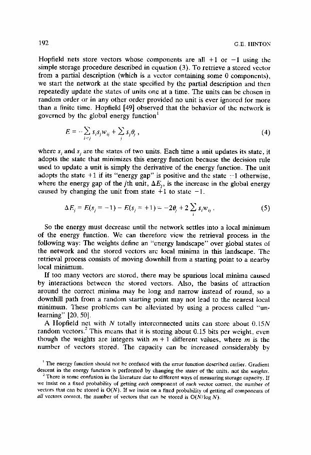
Hopfield nets store vectors whose components are all +1 or - 1 using the simple storage procedure described in equation (3). To retrieve a stored vector from a partial description (which is a vector containing some 0 components) , we start the network at the state specified by the partial description and then repeatedly update the states of units one at a time. The units can be chosen in random order or in any other order provided no unit is ever ignored for more than a finite time. Hopfield [49] observed that the behavior of the network is governed by the global energy function t

E "= - - E SiSjWij q- E sjOj, (4) i<j j

where s i and sj are the states of two units. Each time a unit updates its state, it adopts the state that minimizes this energy function because the decision rule used to update a unit is simply the derivative of the energy function. The unit adopts the state + 1 if its "energy gap" is positive and the state - 1 otherwise, where the energy gap of the j th unit, AEj, is the increase in the global energy caused by changing the unit from state + 1 to state - 1 .

a G = E(% = - 1 ) - E(sj = + 1 ) = -2O,. + 2 ~ s,w,. (5) i

So the energy must decrease until the network settles into a local minimum of the energy function. We can therefore view the retrieval process in the following way: The weights define an "energy landscape" over global states of the network and the stored vectors are local minima in this landscape. The retrieval process consists of moving downhill from a starting point to a nearby local minimum.

If too many vectors are stored, there may be spurious local minima caused by interactions between the stored vectors. Also, the basins of attraction around the correct minima may be long and narrow instead of round, so a downhill path from a random starting point may not lead to the nearest local minimum. These problems can be alleviated by using a process called "unlearning" [20, 50].

A Hopfield net with N totally interconnected units can store about 0.15N random vectors. 2 This means that it is storing about 0.15 bits per weight, even though the weights are integers with m + 1 different values, where m is the number of vectors stored. The capacity can be increased considerably by

' The energy function should not be confused with the error function described earlier. Gradient descent in the energy funct ion is per formed by changing the states of the units, not the weights.

2 There is some confusion in the literature due to different ways of measur ing storage capacity. If we insist on a fixed probability of getting each componen t of each vector correct, the number of vectors that can be stored is O(N) . If we insist on a fixed probability of getting all components of a / /vec tors correct, the n u m b e r of vectors that can be stored is O(N/ log N).


abandoning the one-shot storage procedure and explicitly training the network on typical noisy retrieval tasks using the threshold least squares or perceptron convergence procedures described below.

4.3. The deficiencies of associators without hidden units

If the input vectors are orthogonal, or if they are made to be close to orthogonal by using high-dimensional random vectors (as is typically done in a Hopfield net), associators with no hidden units perform well using a simple Hebbian storage procedure. If the set of input vectors satisfy the much weaker condition of being linearly independent, associators with no hidden units can learn to give the correct outputs provided an iterative learning procedure is used. Unfortunately, linear independence does not hold for most tasks that can be characterized as mapping input vectors to output vectors because the number of relevant input vectors is typically much larger than the number of components in each input vector. The required mapping typically has a complicated structure that can only be expressed using multiple layers of hidden units. 3 Consider, for example, the task of identifying an object when the input vector is an intensity array and the output vector has a separate component for each possible name. If a given type of object can be either black or white, the intensity of an individual pixel (which is what an input unit encodes) cannot provide any direct evidence for the presence or absence of an object of that type. So the object cannot be identified by using weights on direct connections from input to output units. Obviously, it is necessary to explictly extract relationships among intensity values (such as edges) before trying to identify the object. Actually, extracting edges is just a small part of the problem. If recognition is to have the generative capacity to handle novel images of familiar objects the network must somehow encode the systematic effects of variations in lighting and viewpoint, partial occlusion by other objects, and deformations of the object itself. There is a tremendous gap between these complex regularities and the regularities that can be captured by an associative net that lacks hidden units.

5. Simple Supervised Learning Procedures

Consider a network that has input units which are directly connected to output units whose states (i.e. activity levels) are a continuous smooth function of their total input. Suppose that we want to train the network to produce particular "desired" states of the output units for each member of a set of input vectors. A measure of how poorly the network is performing with its current

3 It is always possible to redefine the units and the connectivity so that multiple layers of simple units become a single layer of much more complicated units. But this redefinition does not make the problem go away.

194 G.E. HINTON

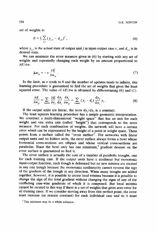
set of weights is:

E = ½ ~ (Y~,c - dj,c) 2 , ( 6 ) j ,c

where Yj,c is the actual state of output unit j in input-output case c, and dj, c is its desired state.

We can minimize the error measure given in (6) by starting with any set of weights and repeatedly changing each weight by an amount proportional to OE/Ow.

OE a w j , = - e awj----~ " ( 7 )

In the limit, as e tends to 0 and the number of updates tends to infinity, this learning procedure is guaranteed to find the set of weights that gives the least squared error. The value of aE/Ow is obtained by differentiating (6) and (1).

OE = ~, OE dY i Oxj _ ~ ( y j - d j ) dy~ OWji c a s e s Oyj dxj Ow~i .... s ~ Yi" (8)

If the output units are linear, the term dy/dx j is a constant. The least squares learning procedure has a simple geometric interpretation.

We construct a multi-dimensional "weight space" that has an axis for each weight and one extra axis (called "height") that corresponds to the error measure. For each combination of weights, the network will have a certain error which can be represented by the height of a point in weight space. These points form a surface called the "error surface". For networks with linear output units and no hidden units, the error surface always forms a bowl whose horizontal cross-sections are ellipses and whose vertical cross-sections are parabolas. Since the bowl only has one minimum, 4 gradient descent on the error surface is guaranteed to find it.

The error surface is actually the sum of a number of parabolic troughs, one for each training case. If the output units have a nonlinear but monotonic input-output function, each trough is deformed but no new minima are created in any one trough because the monotonic nonlinearity cannot reverse the sign of the gradient of the trough in any direction. When many troughs are added together, however, it is possible to create local minima because it is possible to change the sign of the total gradient without changing the signs of any of the conflicting case-wise gradients of which it is composed. But local minima cannot be created in this way if there is a set of weights that gives zero error for all training cases. If we consider moving away from this perfect point, the error must increase (or remain constant) for each individual case and so it must

4 This minimum may be a whole subspace.


increase (or remain constant) for the sum of all these cases. So gradient descent is still guaranteed to work for monotonic nonlinear input-output functions provided a perfect solution exists. However , it will be very slow at points in weight space where the gradient of the input-output function approaches zero for the output units that are in error.

The "batch" version of the least squares procedure sweeps through all the cases accumulating OE/Ow before changing the weights, and so it is guaranteed to move in the direction of steepest descent. The "onl ine" version, which requires less memory, updates the weights after each input-output case [99]. 5 This may sometimes increase the total error, E, but by making the weight changes sufficiently small the total change in the weights after a complete sweep through all the cases can be made to approximate steepest descent arbitrarily closely.

5.1. A least squares procedure for binary threshold units

Binary threshold units use a step function, so the term dy / /dx / i s infinite at the threshold and zero elsewhere and the least squares procedure must be modified to be applicable to these units. In the following discussion we assume that the threshold is implemented by a "bias" weight on a permanently active input line, so the unit turns on if its total input exceeds zero. The basic idea is to define an error function that is large if the total input is far from zero and the unit is in the wrong state and is 0 when the unit is in the right state. The simplest version of this idea is to define the error of an output unit, j for a given input case to be

r 0 , if output unit has the fight s ta te ,

Ej,~* -- ~ 1x2 if output unit has the wrong state l ~ j , c ,

Unfortunately, this measure can be minimized by setting all weights and biases to zero so that units are always exactly at their threshold (Yann Le Cun, personal communication). To avoid this problem we can introduce a margin, m, and insist that for units which should be on the total input is at least m and for units that should be of f the total input is at most - m . The new error measure is then

E j,c I 0 , = l ( m - xj,c) 2 ,

1½(m + X j , c ) 2 ,

if output unit has the fight state by at least m ,

if output unit should be on but has x j, c < m ,

if output unit should be off but has xj. c > - m .

s The online version is usually called the "least mean squares" or "LMS" procedure.

196 G.E. HINTON

The derivative of this error measure with respect to xj, c is

0, O E j*,c

- x j, c - m , OXj'c x/, c + m ;

if output unit has the right state by at least m ,

if output unit should be on but has xj,~ < rn,

if output unit should be off but has xj,~ > - m .

So the "threshold least squares procedure" becomes:

3 E j* c A w j i = - e ~c ~Xy,c Yi,c "

5.2. The perceptron convergence procedure

One version of the perceptron convergence procedure is related to the online version of the threshold least squares procedure in the following way: The magnitude of O E ~ c / O x j , ~ is ignored and only its sign is taken into consideration. So the weight changes are:

m w j i , c {! : e y i , c ,

e Y i , c ,

if output unit behaves correctly by at least m ,

if output unit should be on but has xj, c < m ,

if output unit should be off but has xj,c > - m .

Because it ignores the magnitude of the error, this procedure changes weights by at least e even when the error is very small. The finite size of the weight steps eliminates the need for a margin so the standard version of the perceptron convergence procedure does not use one.

Because it ignores the magnitude of the error this procedure does not even stochastically approximate steepest descent in E, the sum squared error. Even with very small e, it is quite possible for E to rise after a complete sweep through all the cases. However, each time the weights are updated, the perceptron convergence procedure is guaranteed to reduce the value of a different cost measure that is defined solely in terms of weights.

To picture the least squares procedure we introduced a space with one dimension for each weight and one extra dimension for the sum squared error in the output vectors. To picture the perceptron convergence procedure, we do not need the extra dimension for the error. For simplicity we shall consider a network with only one output unit. Each case corresponds to a constraint hyperplane in weight space. If the weights are on one side of this hyperplane, the output unit will behave correctly and if they are on the other side it will behave incorrectly (see Fig. 3). To behave correctly for all cases, the weights


V

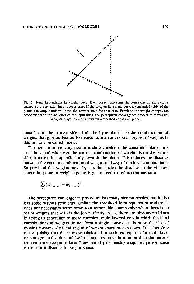
Fig. 3. Some hyperplanes in weight space. Each plane represents the constraint on the weights caused by a particular input-output case. If the weights lie on the correct (unshaded) side of the plane, the output unit will have the correct state for that case. Provided the weight changes are proportional to the activities of the input lines, the perceptron convergence procedure moves the

weights perpendicularly towards a violated constraint plane.

must lie on the correct side of all the hyperplanes, so the combinations of weights that give perfect performance form a convex set. Any set of weights in this set will be called "ideal."

The perceptron convergence procedure considers the constraint planes one at a time, and whenever the current combination of weights is on the wrong side, it moves it perpendicularly towards the plane. This reduces the distance between the current combination of weights and any of the ideal combinations. So provided the weights move by less than twice the distance to the violated constraint plane, a weight update is guaranteed to reduce the measure

'~ (Wi,actual W . 2

-- /,ideal) i

The perceptron convergence procedure has many nice properties, but it also has some serious problems. Unlike the threshold least squares procedure, it does not necessarily settle down to a reasonable compromise when there is no set of weights that will do the job perfectly. Also, there are obvious problems in trying to generalize to more complex, multi-layered nets in which the ideal combinations of weights do not form a single convex set, because the idea of moving towards the ideal region of weight space breaks down. It is therefore not surprising that the more sophisticated procedures required for multi-layer nets are generalizations of the least squares procedure rather than the perceptron convergence procedure: They learn by decreasing a squared performance error, not a distance in weight space.

198 G.E. HINTON

5.3. The deficiencies of simple learning procedures

The major deficiency of both the least squares and perceptron convergence procedures is that most "interesting" mappings between input and output vectors cannot be captured by any combination of weights in such simple networks, so the guarantee that the learning procedure will find the best possible combination of weights is of little value. Consider, for example, a network composed of two input units and one output unit. There is no way of setting the two weights and one threshold to solve the very simple task of producing an output of 1 when the input vector is (1, 1) or (0, 0) and an output of 0 when the input vector is (1, 0) or (0, 1). Minsky and Papert [68] give a clear analysis of the limitations on what mappings can be computed by three-layered nets. They focus on the question of what preprocessing must be done by the units in the intermediate layer to allow a task to be solved. They generally assume that the preprocessing is fixed, and so they avoid the problem of how to make the units in the intermediate layer learn useful predicates. So, from the learning perspective, their intermediate units are not true hidden units.

Another deficiency of the least squares and perceptron learning procedures is that gradient descent may be very slow if the elliptical cross-section of the error surface is very elongated so that the surface forms a long ravine with steep sides and a very low gradient along the ravine. In this case, the gradient at most points in the space is almost perpendicular to the direction towards the minimum. If the coefficient e in (7) is large, there are divergent oscillations across the ravine, and if it is small the progress along the ravine is very slow. A standard method for speeding the convergence in such cases is recursive least squares [100]. Various other methods have also been suggested [5, 71, 75].

We now consider learning in more complex networks that contain hidden units. The next five sections describe a variety of supervised, unsupervised, and reinforcement learning procedures for these nets.

6. Backpropagation: A Multi-layer Least Squares Procedure

The "backpropagation" learning procedure [80, 81] is a generalization of the least squares procedure that works for networks which have layers of hidden units between the input and output units. These multi-layer networks can compute much more complicated functions than networks that lack hidden units, but the learning is generally much slower because it must explore the space of possible ways of using the hidden units. There are now many examples in which backpropagation constructs interesting internal representations in the hidden units, and these representations allow the network to generalize in sensible ways. Variants of the procedure were discovered independently by Werbos [98], Le Cun [59] and Parker [70].

In a multi-layer network it is possible, using (8), to compute OE/Owji for all


the weights in the network provided we can compute OE/Oy/for all the units that have modifiable incoming weights. In a system that has no hidden units, this is easy because the only relevant units are the output units, and for them OE/Oy~ is found by differentiating the error function in (6). But for hidden units, OE/Oy/is harder to compute. The central idea of backpropagation is that these derivatives can be computed efficiently by starting with the output layer and working backwards through the layers. For each input-output case, c, we first use a forward pass, starting at the input units, to compute the activity levels of all the units in the network. Then we use a backward pass, starting at the output units, to compute OE/Oyj for all the hidden units. For a hidden unit, j, in layer J the only way it can affect the error is via its effects on the units, k, in the next layer, K (assuming units in one layer only send their outputs to units in the layer above). So we have

OE - ~_~k OE dYk dXk = ~k OE dyk Oy/ Oy k dx k dy/ Oy k dx k Wkj , (9)

where the index c has been suppressed for clarity. So if OE/Oy k is already known for all units in layer K, it is easy to compute the same quantity for units in layer J. Notice that the computation performed during the backward pass is very similar in form to the computation performed during the forward pass (though it propagates error derivatives instead of activity levels, and it is entirely linear in the error derivatives).

6.1. The shape of the error surface

In networks without hidden units, the error surface only has one minimum (provided a perfect solution exists and the units use smooth monotonic input-output functions). With hidden units, the error surface may contain many local minima, so it is possible that steepest descent in weight space will get stuck at poor local minima. In practice, this does not seem to be a serious problem. Backpropagation has been tried for a wide variety of tasks and poor local minima are rarely encountered, provided the network contains a few more units and connections than are required for the task. One reason for this is that there are typically a very large number of qualitatively different perfect solutions, so we avoid the typical combinatorial optimization task in which one minimum is slightly better than a large number of other, widely separated minima.

In practice, the most serious problem is the speed of convergence, not the presence of nonglobal minima. This is discussed further in Section 12.

6.2. Backpropagation for discovering semantic features

To demonstrate the ability of backpropagation to discover important underlying features of a domain, Hinton [38] used a multi-layer network to learn the

200 G.E. HINTON

Christopher = Penelope Andrew = Christine I I

I t 1 I Margaret = Arthur Victode = James Jennifer = Charles

i I I

Colin Charlotte

Roberto = Maria Pierro = Francesca t 1

I I I I Gina = Emilio Lucia = Marco Angela = Tomaso

1 I 1

Alfonso Sophie

Fig. 4. Two isomorphic family trees.

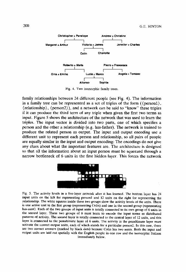
family relationships between 24 different people (see Fig. 4). The information in a family tree can be represented as a set of triples of the form ((personl) , (relationship), (person2)), and a network can be said to "know" these triples if it can produce the third term of any triple when given the first two terms as input. Figure 5 shows the architecture of the network that was used to learn the triples. The input vector is divided into two parts, one of which specifies a person and the other a relationship (e.g. has-father). The network is trained to produce the related person as output. The input and output encoding use a different unit to represent each person and relationship, so all pairs of people are equally similar in the input and output encoding: The encodings do not give any clues about what the important features are. The architecture is designed so that all the information about an input person must be squeezed through a narrow bottleneck of 6 units in the first hidden layer. This forces the network

Fig. 5. The activity levels in a five-layer network after it has learned. The bottom layer has 24 input units on the left for representing person1 and 12 units on the right for representing the relationship. The white squares inside these two groups show the activity levels of the units. There is one active unit in the first group (representing Colin) and one in the second group (representing has-aunt). Each of the two groups of input units is totally connected to its own group of 6 units in the second layer. These two groups of 6 must learn to encode the input terms as distributed patterns of activity. The second layer is totally connected to the central layer of 12 units, and this layer is connected to the penultimate layer of 6 units. The activity in the penultimate layer must activate the correct output units, each of which stands for a particular person2. In this case, there are two correct answers (marked by black dots) because Colin has two aunts. Both the input and output units are laid out spatially with the English people in one row and the isomorphic Italians

immediately below.


to represent people using distributed patterns of activity in this layer. The aim of the simulation is to see if the components of these distributed patterns correspond to the important underlying features of the domain.

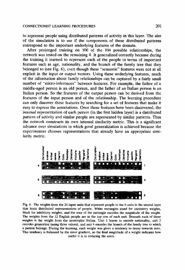
After prolonged training on 100 of the 104 possible relationships, the network was tested on the remaining 4. It generalized correctly because during the training it learned to represent each of the people in terms of important features such as age, nationality, and the branch of the family tree that they belonged to (see Fig. 6), even though these "semantic" features were not at all explicit in the input or output vectors. Using these underlying features, much of the information about family relationships can be captured by a fairly small number of "micro-inferences" between features. For example, the father of a middle-aged person is an old person, and the father of an Italian person is an Italian person. So the features of the output person can be derived from the features of the input person and of the relationship. The learning procedure can only discover these features by searching for a set of features that make it easy to express the associations. Once these features have been discovered, the internal representation of each person (in the first hidden layer) is a distributed pattern of activity and similar people are represented by similar patterns. Thus the network constructs its own internal similarity metric. This is a significant advance over simulations in which good generalization is achieved because the experimenter chooses representations that already have an appropriate similarity metric.

l ~ _ ~ l l W ̧ ~ ~ ~ - ~

Fig. 6. The weights from the 24 input units that represent people to the 6 units in the second layer that learn distributed representations of people. White rectangles stand for excitatory weights, black for inhibitory weights, and the area of the rectangle encodes the magnitude of the weight. The weights from the 12 English people are in the top row of each unit. Beneath each of these weights is the weight from the isomorphic Italian. Unit 1 learns to encode nationality, unit 2 encodes generation (using three values), and unit 4 encodes the branch of the family tree to which a person belongs. During the learning, each weight was given a tendency to decay towards zero. This tendency is balanced by the error gradient, so the final magnitude of a weight indicates how

useful it is in reducing the error.

2 0 2 G.E. H I N T O N

6.3. Backpropagation for mapping text to speech

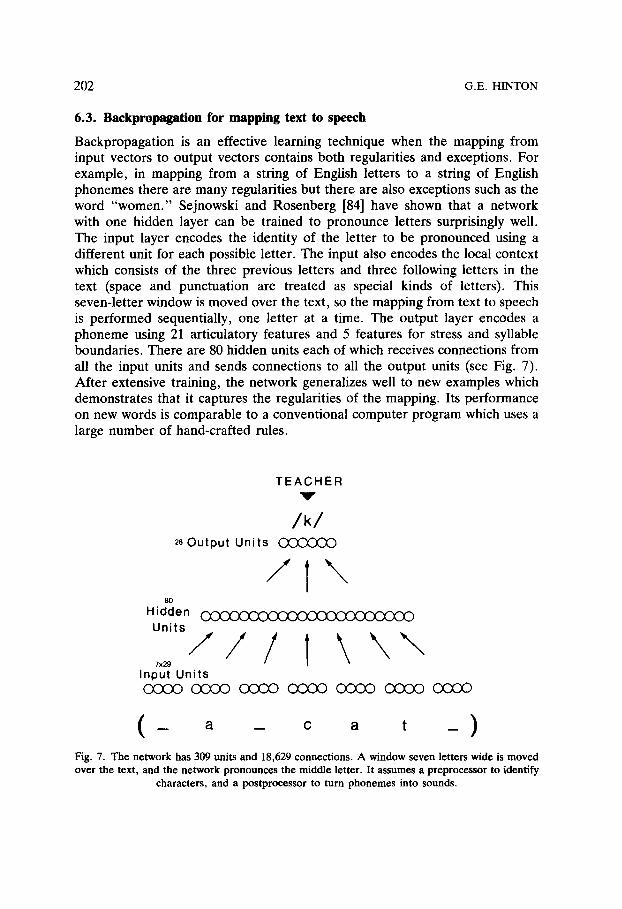
Backpropagation is an effective learning technique when the mapping from input vectors to output vectors contains both regularities and exceptions. For example, in mapping from a string of English letters to a string of English phonemes there are many regularities but there are also exceptions such as the word "women." Sejnowski and Rosenberg [84] have shown that a network with one hidden layer can be trained to pronounce letters surprisingly well. The input layer encodes the identity of the letter to be pronounced using a different unit for each possible letter. The input also encodes the local context which consists of the three previous letters and three following letters in the text (space and punctuation are treated as special kinds of letters). This seven-letter window is moved over the text, so the mapping from text to speech is performed sequentially, one letter at a time. The output layer encodes a phoneme using 21 articulatory features and 5 features for stress and syllable boundaries. There are 80 hidden units each of which receives connections from all the input units and sends connections to all the output units (see Fig. 7). After extensive training, the network generalizes well to new examples which demonstrates that it captures the regularities of the mapping. Its performance on new words is comparable to a conventional computer program which uses a large number of hand-crafted rules.

TEACHER 'V"

/ k / 26 Output Units

/T", 80

Hidden Units l \ \ ' , , ,

Input Units ~ OOOO C O £ ~ OOOO OOCO OOCO OCx30

_ a _ c a t _ )

Fig. 7. The network has 309 units and 18,629 connections. A window seven letters wide is moved over the text, and the network pronounces the middle letter. It assumes a preprocessor to identify

characters, and a postprocessor to turn phonemes into sounds.


6.4. Backpropagation for phoneme recognition

Speech recognition is a task that can be used to assess the usefulness of backpropagation for real-world signal-processing applications. The best existing techniques, such as hidden Markov models [9], are significantly worse than people, and an improvement in the quality of recognition would be of great practical significance.

A subtask which is well-suited to backpropagation is the bottom-up recognition of highly confusable consonants. One obvious approach is to convert the sound into a spectrogram which is then presented as the input vector to a multi-layer network whose output units represent different consonants. Un- fortunately, this approach has two serious drawbacks. First, the spectrogram must have many "pixels" to give reasonable resolution in time and frequency, so each hidden unit has many incoming weights. This means that a very large number of training examples are needed to provide enough data to estimate the weights. Second, it is hard to achieve precise time alignment of the input data, so the spatial pattern that represents a given phoneme may occur at many different positions in the spectrogram. To learn that these shifts in position do not change the identity of the phoneme requires an immense amount of training data. We already know that the task has a certain symmetry--the same sounds occurring at different times mean the same phoneme. To speed learning and improve generalization we should build this a priori knowledge into the network and let it use the information in the training data to discover structure that we do not already understand.

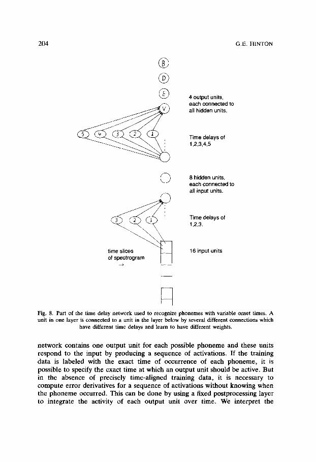
An interesting way to build in the time symmetry is to use a multi-layer, feed-forward network that has connections with time delays [88]. The input units represent a single time flame from the spectrogram and the whole spectrogram is represented by stepping it through the input units. Each hidden unit is connected to each unit in the layer below by several different connections with different time delays and different weights. So it has a limited temporal window within which it can detect temporal patterns in the activities of the units in the layer below. Since a hidden unit applies the same set of weights at different times, it inevitably produces similar responses to similar patterns that are shifted in time (see Fig. 8).

Kevin Lang [58] has shown that a time delay net that is trained using a generalization of the backpropagation procedure compares favorably with hidden Markov models at the task of distinguishing the words "bee", "dee", "ee", and "vee" spoken by many different male speakers in a very noisy environment. Waibel et al. [97] have shown that the same network can achieve excellent speaker-dependent discrimination of the phonemes "b", "d", and "g" in varying phonetic contexts.

An interesting technical problem arises in computing the error derivatives for the output units of the time delay network. The adaptive part of the

204 G.E. HINTON

@

©

time slices of spectrogram

4 output units, each connected to all hidden units.

Time delays of 1,2,3,4,5

8 hidden units, each connected to all input units.

Time delays of 1,2,3.

16 input units

Fig. 8. Part of the time delay network used to recognize phonemes with variable onset times. A unit in one layer is connected to a unit in the layer below by several different connections which

have different time delays and learn to have different weights.

network contains one output unit for each possible phoneme and these units respond to the input by producing a sequence of activations. If the training data is labeled with the exact time of occurrence of each phoneme, it is possible to specify the exact time at which an output unit should be active. But in the absence of precisely time-aligned training data, it is necessary to compute error derivatives for a sequence of activations without knowing when the phoneme occurred. This can be done by using a fixed postprocessing layer to integrate the activity of each output unit over time. We interpret the


instantaneous activity of an output unit as a representation of the probability that the phoneme occurred at exactly that time. So, for the phoneme that really occurred, we know that the time integral of its activity should be 1 and for the other phonemes it should be 0. So at each time, the error derivative is simply the difference between the desired and the actual integral. After training, the network localizes phonemes in time, even though the training data contains no information about time alignment.

6.5. Postprocessing the output of a backpropagation net

Many people have suggested transforming the raw input vector with a module that uses unsupervised learning before presenting it to a module that uses supervised learning. It is less obvious that a supervised module can also benefit from a nonadaptive postprocessing module. A very simple example of this kind of postprocessing occurs in the time delay phoneme recognition network described in Section 6.4.

David Rumelhart has shown that the idea of a postprocessing module can be applied even in cases where the postprocessing function is initially unknown. In trying to imitate a sound, for example, a network might produce an output vector which specifies how to move the speech articulators. This output vector needs to be postprocessed to turn it into a sound, but the postprocessing is normally done by physics. Suppose that the network does not receive any direct information about what it should do with its articulators but it does "know" the desired sound and the actual sound, which is the transformed "image" of the output vector. If we had a postprocessing module which transformed the activations of the speech articulators into sounds, we could backpropagate through this module to compute error derivatives for the articulator activations.

Rumelhart uses an additional network (which he calls a mental model) that first learns to perform the postprocessing (i.e. it learns to map from output vectors to their transformed images). Once this mapping has been learned, backpropagation through the mental model can convert error derivatives for the "images" into error derivatives for the output vectors of the basic network.

6.6. A reinforcement version of backpropagation

Munro [69] has shown that the idea of using a mental model can be applied even when the image of an output vector is simply a single scalar value--the reinforcement. First, the mental model learns to predict expected reinforcement from the combination of the input vector and the output vector. Then the derivative of the expected reinforcement can be backpropagated through the mental model to get the reinforcement derivatives for each component of the output vector of the basic network.

206 G.E. HINTON

6.7. Iterative backpropagation

Rumelhart, Hinton, and Williams [80] show how the backpropagation procedure can be applied to iterative networks in which there are no limitations on the connectivity. A network in which the states of the units at time t determine the states of the units at time t + 1 is equivalent to a net which has one layer for each time slice. Each weight in the iterative network is implemented by a whole set of identical weights in the corresponding layered net, one for each time slice (see Fig. 9). In the iterative net, the error is typically the difference between the actual and desired final states of the network, and to compute the error derivatives it is necessary to backpropagate through time, so the history of states of each unit must be stored. Each weight will have many different error derivatives, one for each time step, and the sum of all these derivatives is used to determine the weight change.

Backpropagation in iterative nets can be used to train a network to generate sequences or to recognize sequences or to complete sequences. Examples are given by Rumelhart, Hinton and Williams [81]. Alternatively, it can be used to store a set of patterns by constructing a point attractor for each pattern. Unlike the simple storage procedure used in a Hopfield net, or the more sophisticated storage procedure used in a Boltzmann machine (see Section 7), backpropagation takes into account the path used to reach a point attractor. So it will not construct attractors that cannot be reached from the normal range of starting points on which it is trained. 6

Fig. 9. On the left is a simple iterative network that is run synchronously for three iterations. On the right is the equivalent layered network.

6A backpropagation net that uses asymmetric connections (and synchronous updating) is not guaranteed to settle to a single stable state. To encourage it to construct a point attractor, rather than a limit cycle, the point attractor can be made the desired state for the last few iterations.


6.8. Backpropagation as a maximum likelihood procedure

If we interpret each output vector as a specification of a conditional probability distribution over a set of output vectors given an input vector, we can interpret the backpropagation learning procedure as a method of finding weights that maximize the likelihood of generating the desired conditional probability distributions. Two examples of this kind of interpretation will be described.

Suppose we only attach meaning to binary output vectors and we treat a real-valued output vector as a way of specifying a probability distribution over binary vectors. We imagine that a real-valued output vector is stochastically converted into a binary vector by treating the real values as the probabilities that individual components have value 1, and assuming independence between components. For simplicity, we can assume that the desired vectors used during training are binary vectors, though this is not necessary. Given a set of training cases, it can be shown that the likelihood of producing exactly the desired vectors is maximized when we minimize the cross-entropy, C, between the desired and actual conditional probability distributions:

C = - ~ dj, c log2(Yj,c) + (1 - djx ) log2(1 - Yj,c), j,c

where dj,~ is the desired probability of output unit j in case c and Yjx is its actual probability.

So, under this interpretation of the output vectors, we should use the cross-entropy function rather than the squared difference as our cost measure. In practice, this helps to avoid a problem caused by output units which are firmly off when they should be on (or vice versa). These units have a very small value of Oy/Ox so they need a large value of OE/Oy in order to change their incoming weights by a reasonable amount. When an output unit that should have an activity level of 1 changes from a level of 0.0001 to level of 0.001, the squared difference from 1 only changes slightly, but the cross-entropy decreases a lot. In fact, when the derivative of the cross-entropy is multiplied by the derivative of the logistic activation function, the product is simply the difference between the desired and the actual outputs, so OCj,c/Oxj, c is just the same as for a linear output unit (Steven Nowlan, personal communication).

This way of interpreting backpropagation raises the issue of whether, under some other interpretation of the output vectors, the squared error might not be the correct measure for performing maximum likelihood estimation. In fact, Richard Golden [32] has shown that minimizing the squared error is equivalent to maximum likelihood estimation if both the actual and the desired output vectors are treated as the centers of Gaussian probability density functions over the space of all real vectors. So the "correct" choice of cost function depends on the way the output vectors are most naturally interpreted.

Both the examples of baekpropagation described above fit this interpretation.

208 G.E. HINTON

6.9. Self-supervised backpropagation

One drawback of the standard form of backpropagation is that it requires an external supervisor to specify the desired states of the output units (or a transformed "image" of the desired states). It can be converted into an unsupervised procedure by using the input itself to do the supervision, using a multi-layer "encoder" network [2] in which the desired output vector is identical with the input vector. The network must learn to compute an approximation to the identity mapping for all the input vectors in its training set, and if the middle layer of the network contains fewer units than the input layer, the learning procedure must construct a compact, invertible code for each input vector. This code can then be used as the input to later stages of processing.

The use of self-supervised backpropagation to construct compact codes resembles the use of principal components analysis to perform dimensionality reduction, but it has the advantage that it allows the code to be a nonlinear transform of the input vector. This form of backpropagation has been used successfully to compress images [19] and to compress speech waves [25]. A variation of it has been used to extract the underlying degrees of freedom of simple shapes [83].

It is also possible to use backpropagation to predict one part of the perceptual input from other parts. For example, in predicting one patch of an image from neighboring patches it is probably helpful to use hidden units that explicitly extract edges, so this might be an unsupervised way of discovering edge detectors. In domains with sequential structure, one portion of a sequence can be used as input and the next term in the sequence can be the desired output. This forces the network to extract features that are good predictors. If this is applied to the speech wave, the states of the hidden units will form a nonlinear predictive code. It is not yet known whether such codes are more helpful for speech recognition than linear predictive coefficients.

A different variation of self-supervised backpropagation is to insist that all or part of the code in the middle layer change as slowly as possible with time. This can be done by making the desired state of each of the middle units be the state it actually adopted for the previous input vector. This forces the network to use similar codes for input vectors that occur at neighboring times, which is a sensible principle if the input vectors are generated by a process whose underlying parameters change more slowly than the input vectors themselves.

6.10. The deficiencies of backpropagation

Despite its impressive performance on relatively small problems, and its promise as a widely applicable mechanism for extracting the underlying structure of a domain, backpropagation is inadequate, in its current form, for larger tasks because the learning time scales poorly. Empirically, the learning

C O N N E C T I O N I S T L E A R N I N G P R O C E D U R E S 209

time on a serial machine is very approximately O(N 3) where N is the number of weights in the network. The time for one forward and one backward pass is O(N). The number of training examples is typically O(N), assuming the amount of information per output vector is held constant and enough training cases are used to strain the storage capacity of the network (which is about 2 bits per weight). The number of times the weights must be updated is also approximately O(N). This is an empirical observation and depends on the nature of the task. 8 On a parallel machine that used a separate processor for

• • • 2 each connecUon, the Ume would be reduced to approximately O(N ). Back- propagation can probably be improved by using the gradient information in more sophisticated ways, but much bigger improvements are likely to result from making better use of modularity (see Section 12.4).

As a biological model, backpropagation is implausible. There is no evidence that synapses can be used in the reverse direction, or that neurons can propagate error derivatives backwards (using a linear input-output function) as well as propagating activity levels forwards using a nonlinear input-output function. One approach is to try to backpropagate the derivatives using separate circuitry that learns to have the same weights as the forward circuitry [70]. A second approach, which seems to be feasible for self-supervised backpropagation, is to use a method called "recirculation" that approximates gradient descent and is more biologically plausible [41]. At present, backpropagation should be treated as a mechanism for demonstrating the kind of learning that can be done using gradient descent, without implying that the brain does gradient descent in the same way.

7. Boltzmann Machines

A Boltzmann machine [2, 46] is a generalization of a Hopfield net (see Section 4.2) in which the units update their states according to a stochastic decision rule. The units have states of 1 or 0, 9 and the probability that unit j adopts the state 1 is given by

1 PJ - 1 + e -aE/r ' (10)

where AE~=x) is the total input received by the jth unit and T is the "temperature." It can be shown that if this rule is applied repeatedly to the units, the network will reach "thermal equilibrium." At thermal equilibrium the units still change state, but the probability of finding the network in any

8 Tesauro [90] reports a case in which the n u m b e r of weight updates is roughly proport ional to the n u m b e r of training cases (it is actually a 4/3 power law). Judd shows that in the worst case it is exponent ial [53].

9 A network that uses states of 1 and 0 can always be converted into an equivalent network that uses states of +1 and - 1 provided the thresholds are altered appropriately.

210 G.E. HINTON

global state remains constant and obeys a Boltzmann distribution in which the probability ratio of any two global states depends solely on their energy difference:

PA - - = e - - ( E A - - E B ) / T .

PB

At high temperature, the network approaches equilibrium rapidly but low energy states are not much more probable than high energy states. At low temperature the network approaches equilibrium more slowly, but low energy states are much more probable than high energy states. The fastest way to approach low temperature equilibrium is generally to start at a high temperature and to gradually reduce the temperature. This is called "simulated annealing" [55]. Simulated annealing allows Boltzmann machines to find low energy states with high probability. If some units are clamped to represent an input vector, and if the weights in the network represent the constraints of the task domain, the network can settle on a very plausible output vector given the current weights and the current input vector.

For complex tasks there is generally no way of expressing the constraints by using weights on pairwise connections between the input and output units. It is necessary to use hidden units that represent higher-order features of the domain. This creates a problem: Given a limited number of hidden units, what higher-order features should they represent in order to approximate the required input-output mapping as closely as possible? The beauty of Boltzmann machines is that the simplicity of the Boltzmann distribution leads to a very simple learning procedure which adjusts the weights so as to use the hidden units in an optimal way.

The network is "shown" the mapping that it is required to perform by clamping an input vector on the input units and clamping the required output vector on the output units. If there are several possible output vectors for a given input vector, each of the possibilities is clamped on the output units with the appropriate frequency. The network is then annealed until it approaches thermal equilibrium at a temperature of 1. It then runs for a fixed time at equilibrium and each connection measures the fraction of the time during which both the units it connects are active. This is repeated for all the various input-output pairs so that each connection can measure (sis/)÷, the expected probability, averaged over all cases, that unit i and unit j are simultaneously active at thermal equilibrium when the input and output vectors are both clamped.

The network must also be run in just the same way but without clamping the output units. Again, it reaches thermal equilibrium with each input vector clamped and then runs for a fixed additional time to m e a s u r e ~sisj~-, the expected probability that both units are active at thermal equilibrium when the


output vector is determined by the network. Each weight is then updated by an amount proportional to the difference between these two quantities

a w l s = + -

It has been shown [2] that if e is sufficiently small this performs gradient descent in an information-theoretic measure, G, of the difference between the behavior of the output units when they are clamped and their behavior when they are not clamped.

V+(O~ I t , ) a = ~ P+(I,,, Oa) log (11)

e-(o lIo) '

w h e r e / , is a state vector over the input units, Oa is a state vector over the output units, P+ is a probability measured when both the input and output units are clamped, and P - is a probability measured at thermal equilibrium when only the input units are clamped.

G is called the "asymmetric divergence" or "Kullback information," and its gradient has the same form for connections between input and hidden units, connections between pairs of hidden units, connections between hidden and output units, and connections between pairs of output units. G can be viewed as the difference of two terms. One term is the cross-entropy between the "desired" conditional probability distribution that is clamped on the output units and the "actual" conditional distribution exhibited by the output units when they are not clamped. The other term is the entropy of the "desired" conditional distribution. This entropy cannot be changed by altering the weights, so minimizing G is equivalent to minimizing the cross-entropy term, which means that Boltzmann machines use the same cost function as one form of backpropagation (see Section 6.8).

A special case of the learning procedure is when there are no input units. It can then be viewed as an unsupervised learning procedure which learns to model a probability distribution that is specified by damping vectors on the output units with the appropriate probabilities. The advantage of modeling a distribution in this way is that the network can then perform completion. When a partial vector is clamped over a subset of the output units, the network produces completions on the remaining output units. If the network has learned the training distribution perfectly, its probability of producing each completion is guaranteed to match the environmental conditional probability of this completion given the clamped partial vector.

The learning procedure can easily be generalized to networks where each term in the energy function is the product of a weight, w~,j, k .... and an arbitrary function, f ( i , j, k . . . . ), of the states of a subset of the units. The network must be run so that it achieves a Boltzmann distribution in the energy function, so each unit must be able to compute how the global energy would change if it

212 G.E. HINTON

were to change state. The generalized learning procedure is simply to change the weight by an amount proportional to the difference between ( f( i , j, k , . . . )~÷ and ( f( i , j, k , . . . ) ) - .

The learning procedure using simple pairwise connections has been shown to produce appropriate representations in the hidden units [2] and it has also been used for speech recognition [76]. However, it is considerably slower than backpropagation because of the time required to reach equilibrium in large networks. Also, the process of estimating the gradient introduces several practical problems. If the network does not reach equilibrium the estimated gradient has a systematic error, and if too few samples are taken to estimate (sisj) ÷ and (sisj)- accurately the estimated gradient will be extremely noisy because it is the difference of two noisy estimates. Even when the noise in the estimate of the difference has zero mean, its variance is a function of (s~sj) ÷ and (sisj)-. When these quantities are near zero or one, their estimates will have much lower variance than when they are near 0.5. This nonuniformity in the variance gives the hidden units a surprisingly strong tendency to develop weights that cause them to be on all the time or off all the time. A familiar version of the same effect can be seen if sand is sprinkled on a vibrating sheet of tin. Nearly all the sand clusters at the points that vibrate the least, even though there is no bias in the direction of motion of an individual grain of sand.

One interesting feature of the Boltzmann machine is that it is relatively easy to put it directly onto a chip which has dedicated hardware for each connection and performs the annealing extremely rapidly using analog circuitry that computes the energy gap of a unit by simply allowing the incoming charge to add itself up, and makes stochastic decisions by using physical noise. Alspector and Allen [3] are fabricating a chip which will run about 1 million times as fast as a simulation on a VAX. Such chips may make it possible to apply connectionist learning procedures to practical problems, especially if they are used in conjunction with modular approaches that allow the learning time to scale better with the size of the task.

There is another promising method that reduces the time required to compute the equilibrium distribution and eliminates the noise caused by the sampling errors in (s~sj) ÷ and ~SiSj~-. Instead of directly simulating the stochastic network it is possible to estimate its mean behavior using "mean field theory" which replaces each stochastic binary variable by a deterministic real value that represents the expected value of the stochastic variable. Simulated annealing can then be replaced by a deterministic relaxation procedure that operates on the real-valued parameters [51] and settles to a single state that gives a crude representation of the whole equilibrium distribution. The product of the "activity levels" of two units in this settled state can be used as an approximation of (sis j) so a version of the Boltzmann machine learning procedure can be applied. Peterson and Anderson [74] have shown that this works quite well.


7.1. Maximizing reinforcement and entropy in a Boltzmann machine

The Boltzmann machine learning procedure is based on the simplicity of the expression for the derivative of the asymmetric divergence between the conditional probability distribution exhibited by the output units of a Boltzmann machine and a desired conditional probability distribution. The derivatives of certain other important measures are also very simple if the network is allowed to reach thermal equilibrium. For example, the entropy of the states of the machine is given by

H = - ~ P~ log e P~,

where P,, is the probability of a global configuration, and H is measured in units of log 2 e bits. Its derivative is

OH 1 Ow,~ = T ( ( Es i s j ) - ( E ) ( s i s j ) ) . (12)

So if each weight has access to the global energy, E, it is easy to manipulate the entropy.

It is also easy to perform gradient ascent in expected reinforcement if the network is given a global reinforcement signal, R, that depends on its state. The derivative of the expected reinforcement with respect to each weight is

OR _ 1 ( ( R s i s i ) _ ( R ) ( s i s i ) ) (13) b w o T

A recurrent issue in reinforcement learning procedures is how to trade off short-term optimization of expected reinforcement against the diversity required to discover actions that have a higher reinforcement than the network's current estimate. If we use entropy as a measure of diversity, and we assume that the system tries to optimize some linear combination of the expected reinforcement and the entropy of its actions, it can be shown that its optimal strategy is to pick actions according to a Boltzmann distribution, where the expected reinforcement of a state is the analog of negative energy and the parameter that determines the relative importance of expected reinforcement and diversity is the analog of temperature. This result follows from the fact that the Boltzmann distribution is the one which maximizes entropy (i.e. diversity) for a given expected energy (i.e. reinforcement).

This suggests a learning procedure in which the system represents the expected value of an action by its negative energy, and picks actions by allowing a Boltzmann machine to reach thermal equilibrium. If the weights are updated using equations (12) and (13) the negative energies of states will tend to become proportional to their expected reinforcements, since this is the way to make the derivative of H balance the derivative of R. Once the system has

214 G.E. HINTON

learned to represent the reinforcements correctly, variations in the temperature can be used to make it more or less conservative in its choice of actions whilst always making the optimal tradeoff between diversity and expected reinforcement. Unfortunately, this learning procedure does not make use of the most important property of Boltzmann machines which is their ability to compute the quantity (sisj) given some specified state of the output units. Also, it is much harder to compute the derivative of the entropy if we are only interested in the entropy of the state vectors over the output units.

8. Maximizing Mutual Information: A Semisupervised Learning Procedure

One "semisupervised" method of training a unit is to provide it with information about what category the input vector came from, but to refrain from specifying the state that the unit ought to adopt. Instead, its incoming weights are modified so as to maximize the information that the state of the unit provides about the category of the input vector. The derivative of the mutual information is relatively easy to compute and so it can be maximized by gradient ascent [73]. For difficult discriminations that cannot be performed in a single step this is a good way of producing encodings of the input vector that allow the discrimination to be made more easily. Figure 10 shows an example of a difficult two-way discrimination and illustrates the kinds of discriminant function that maximize the information provided by the state of the unit.

If each unit within a layer independently maximizes the mutual information between its state and the category of the input vector, many units are likely to discover similar, highly correlated features. One way to force the units to diversify is to make each unit receive its inputs from a different subset of the units in the layer below. A second method is to ignore cases in which the input vector is correctly classified by the final output units and to maximize the

+

+ +

- +

4-

- + + -- ~ + + -

- + + + + _ + - +

-4- - - + _ _ +

+ + +

S + _ _4- + +

- ~ + + ~+ +

_ - + +

Fig. 10. (a) There is high mutual information between the state of a binary threshold unit that uses the hyperplane shown and the distribution (+ or - ) that the input vector came from. (b) The probability, given that the unit is on, that the input came from the " + " distribution is not as high using the diagonal hyperplane. However, the unit is on more often. Other things being equal, a

unit conveys most mutual information if it is on half the time.


mutual information between the state of each intermediate unit and the category of the input given that the input is incorrectly classified) °

If the two input distributions that must be discriminated consist of examples taken from some structured domain and examples generated at random (but with the same first-order statistics as the structured domain), this semisupervised procedure will discover higher-order features that characterize the structured domain and so it can be made to act like the type of unsupervised learning procedure described in Section 9.

9. Unsupervised Hebbian Learning

A unit can develop selectivity to certain kinds of features in its ensemble of input vectors by using a simple weight modification procedure that depends on the correlation between the activity of the unit and the activity on each of it input lines. This is called a "Hebbian" learning rule because the weight modification depends on both presynaptic and postsynaptic activity [36]. Typical examples of this kind of learning are described by Cooper, Liberman and Oja [18] and by Bienenstock, Cooper, and Munro [16]. A criticism of early versions of this approach, from a computational point of view, was that the researchers often postulated a simple synaptic modification rule and then explored its consequences rather than rigorously specifying the computational goal and then deriving the appropriate synaptic modification rule. However, an important recent development unifies these two approaches by showing that a relatively simple Hebbian rule can be viewed as the gradient of an interesting function. The function can therefore be viewed as a specification of what the learning is trying to achieve.

9.1. A recent development of unsupervised Hebbian learning

In a recent series of papers Linsker has shown that with proper normalization of the weight changes, an unsupervised Hebbian learning procedure in which the weight change depends on the correlation of presynaptic and postsynaptic activity can produce a surprising number of the known properties of the receptive fields of neurons in visual cortex, including center-surround fields [61], orientation-tuned fields [62] and orientation columns [63]. The procedure operates in a multi-layer network in which there is innate spatial structure so that the inputs to a unit in one layer tend to come from nearby locations in the layer below. Linsker demonstrates that the emergence of biologically sugges- tive receptive fields depends on the relative values of a few generic parameters. He also shows that for each unit, the learning procedure is performing gradient ascent in a measure whose main term is the ensemble average (across all the

10 This method of weighting the statistics by some measure of the overall error or importance of a case can often be used to allow global measures of the performance of the whole network to influence local, unsupervised learning procedures.

216 G.E. HINTON

various patterns of activity in the layer below) of

E WiSiWjS j , i,j

where w i and w/are the weights on the ith and jth input lines of a unit and si and s/are the activities on those input lines.

It is not initially obvious why maximizing the pairwise covariances of the weighted activities produces receptive fields that are useful for visual information processing. Linsker does not discuss this question in his original three papers. However, he has now shown [64] that the learning procedure maximizes the variance in the activity of the postsynaptic unit subject to a "resource" constraint on overall synaptic strength. This is almost equivalent to maximizing the ratio of the postsynaptic variance to the sum of the squares of the weights, which is guaranteed to extract the first principal component (provided the units are linear). This component is the one that would minimize the sum-squared reconstruction error if we tried to reconstruct the activity vector of the presynaptic units from the activity level of the postsynaptic unit. Thus we can view Linsker's learning procedure as a way of ensuring that the activity of a unit conveys as much information as possible about its presynaptic input vector. A similar analysis can be applied to competitive learning (see Section 10).

I0. Competitive Learning

Competitive learning is an unsupervised procedure that divides a set of input vectors into a number of disjoint clusters in such a way that the input vectors within each duster are all similar to one another. It is called competitive learning because there is a set of hidden units which compete with one another to become active. There are many variations of the same basic idea, and only the simplest version is described here. When an input vector is presented to the network, the hidden unit which receives the greatest total input wins the competition and turns on with an activity level of I. All the other hidden units turn off. The winning unit then adds a small fraction of the current input vector to its weight vector. So, in future, it will receive even more total input from this input vector. To prevent the same hidden unit from being the most active in all cases, it is necessary to impose a constraint on each weight vector that keeps the sum of the weights (or the sum of their squares) constant. So when a hidden unit becomes more sensitive to one input vector it becomes less sensitive to other input vectors.

Rumelhart and Zipser [82] present a simple geometrical model of competitive learning. If each input vector has three components and is of unit length it can be represented by a point on the surface of the unit sphere. If the weight vectors of the hidden units are also constrained to be of unit length, they too can be represented by points on the unit sphere as shown in Fig. 11. The


Fig. 11. The input vectors are represented by points marked " x " on the surface of a sphere, The weight vectors of the hidden units are represented by points marked "©." After competitive learning, each weight vector will be close to the center of gravity of a cluster of input vectors.

learning procedure is equivalent to finding the weight vector that is closest to the current input vector, and moving it closer still by an amount that is proportional to the distance. If the weight changes are sufficiently small, this process will stabilize when each weight vector is at the center of gravity of a cluster of input vectors.

We can think of the network as performing the following task: Represent the current input vector, Yc, as accurately as possible by using a single active hidden unit. The representation is simply the weight vector, we, of the hidden unit which is active in case c. If the weight changes are sufficiently small, this version of competitive learning performs steepest descent in a measure of the sum-squared inaccuracy of the representation. The solutions it finds are minima of the function

E = C

Although they use the geometrical analogy described above, Rumelhart and Zipser actually use a slightly different learning rule which cannot be interpreted as performing steepest descent in such a simple error function.

There are many variations of competitive learning in the literature [4, 29, 33, 95] and there is not space here to review them all. A model with similarities to competitive learning has been used by Willshaw and v o n d e r Malsburg [103] to explain the formation of topographic maps between the retina and the tectum. Recently, it has been shown that a variation of this model can be interpreted as performing steepest descent in an error function and can be applied to a range of optimization problems that involve topographic mappings between geometrical structures [23].

218 G.E. HINTON

One major theme has been to show that competitive learning can produce topographic maps [57]. The hidden units are laid out in a spatial structure (usually two-dimensional) and instead of just updating the weight vector of the hidden unit that receives the greatest total input, the procedure also updates the weight vectors of adjacent hidden units. This encourages adjacent units to respond to similar input vectors, and it can be viewed as a way of performing gradient descent in a cost function that has two terms. The first term measures how inaccurately the weight vector of the most active hidden unit represents the input vector. The second term measures the dissimilarity between the input vectors that are represented by adjacent hidden units. Kohonen has shown that this version of competitive learning performs dimensionality reduction, so that surplus degrees of freedom are removed from the input vector and it is represented accurately by a point in a lower-dimensional space [57]. It is not clear how this compares in efficiency with self-supervised backpropagation (see Section 6.9) for dimensionality reduction.

Fukushima and Miyake [30] have demonstrated that a version of competitive learning can be used to allow a multi-layer network to recognize simple two-dimensional shapes in a number of different positions. After learning, the network can recognize a familiar shape in a novel position. The ability to generalize across position depends on using a network in which the layers of units that learn are interleaved with layers of nonlearning units which are prewired to generalize across position. Thus, the network does not truly learn translation invariance. By contrast, it is possible to design a backpropagation network that starts with no knowledge of the effects of translation and no knowledge of which input units are adjacent in the image. After sufficient experience, the network can correctly identify familiar, simple shapes in novel positions [39].

10.1. The relationship between competitive learning and backpropagation

Because it is performing gradient descent in a measure of how accurately the input vector could be reconstructed, competitive learning has a close relationship to self-supervised backpropagation. Consider a three-layer encoder network in which the desired states of the output units are the same as the actual states of the input units. Suppose that each weight from an input unit to a hidden unit is constrained to be identical to the weight from that hidden unit to the corresponding output unit. Suppose, also, that the output units are linear and the hidden units, instead of using the usual nonlinear input-output function, use the same "winner-take-all" nonlinearity as is used in competitive learning. So only one hidden unit will be active at a time, and the actual states of the output units will equal the weights of the active hidden unit. This makes it easy to compute the error derivatives of the weights from the hidden units to the output units. For weights from the active hidden unit the derivatives are


simply proportional to the difference between the actual and desired outputs (which equals the difference between the weight and the corresponding component of the input vector). For weights from inactive hidden units the error derivatives are all zero. So gradient descent can be performed by making the weights of the active hidden unit regress towards the input vector, which is precisely what the competitive learning rule does.

Normally, backpropagation is needed in order to compute the error derivatives of the weights from the input units to the hidden units, but the winner-take-all nonlinearity makes backpropagation unnecessary in this network because all these derivatives are equal to zero. So long as the same hidden unit wins the competition, its activity level is not changed by changing its input weights. At the point where a small change in the weights would change the winner from one hidden unit to another, both hidden units fit the input vector equally well, so changing winners does not alter the total error in the output (even though it may change the output vector a lot). Because the error derivatives are so simple, we can still do the learning if we omit the output units altogether. This removes the output weights, and so we no longer need to constrain the input and output weights of a hidden unit to be identical. Thus the simplified version of competitive learning is a degenerate case of self-supervised backpropagation.

It would be interesting if a mechanism as simple as competitive learning could be used to implement gradient descent in networks that allow the m most activated hidden units to become fully active (where m > 1). This would allow the network to create more complex, distributed representations of the input vectors. Unfortunately the implementation is not nearly as simple because it is no longer possible to omit the output layer. The output units are needed to combine the effects of all the active hidden units and compare the combined effect with the input vector in order to compute the error derivatives of the output weights. Also, at the point at which one hidden unit ceases to be active and another becomes active, there may be a large change in the total error, so at this point there are infinite error derivatives for the weights from the input to the hidden units. It thus appears that the simplicity of the mechanism required for competitive learning is crucially dependent on the fact that only one hidden unit within a group is active.

11. Reinforcement Learning Procedures

There is a large and complex literature on reinforcement learning procedures which is beyond the scope of this paper. The main aim of this section is to give an informal description of a few of the recent ideas in the field that reveals their relationship to other types of connectionist learning.

A central idea in many reinforcement learning procedures is that we can assign credit to a local decision by measuring how it correlates with the global

220 G.E. HINTON

reinforcement signal. Various different values are tried for each local variable (such as a weight or a state), and these variations are correlated with variations in the global reinforcement signal. Normally, the local variations are the result of independent stochastic processes, so if enough samples are taken each local variable can average away the noise caused by the variation in the other variables to reveal its own effect on the global reinforcement signal (given the current average behavior of the other variables). The network can then perform gradient ascent in the expected reinforcement by altering the probability distribution of the value of each local variable in the direction that increases the expected reinforcement. If the probability distributions are altered after each trial, the network performs a stochastic version of gradient ascent.

The main advantage of reinforcement learning is that it is easy to implement because, unlike backpropagation which computes the effect of changing a local variable, the "credit assignment" does not require any special apparatus for computing derivatives. So reinforcement learning can be used in complex systems in which it would be very hard to analytically compute reinforcement derivatives. The main disadvantage of reinforcement learning is that it is very inefficient when there are more than a few local variables. Even in the trivial case when all the local variables contribute independently to the global reinforcement signal, O(NM) trials are required to allow the measured effects of each of the M possible values of a variable to achieve a reasonable signal-to-noise ratio by averaging away the noise caused by the N other variables. So reinforcement learning is very inefficient for large systems unless they are divided into smaller modules. It is as if each person in the United States tried to decide whether he or she had done a useful day's work by observing the gross national product on a day-by-day basis.

A second disadvantage is that gradient ascent may get stuck in local optima. As a network concentrates more and more of its trials on combinations of values that give the highest expected reinforcement, it gets less and less information about the reinforcements caused by other combinations of values.

11.1. Delayed reinforcement

In many real systems, there is a delay between an action and the resultant reinforcement, so in addition to the normal problem of deciding how to assign credit to decisions about hidden variables, there is a temporal credit assignment problem [86]. If, for example, a person wants to know how their behavior affects the gross national product, they need to know whether to correlate today's GNP with what they did yesterday or with what they did five years ago. In the iterative version of backpropagation (Section 6.7), temporal credit assignment is performed by explicitly computing the effect of each activity level on the eventual outcome. In reinforcement learning procedures, temporal


credit assignment is typically performed by learning to associate "secondary" reinforcement values with the states that are intermediate in time between the action and the external reinforcement. One important idea is to make the reinforcement value of an intermediate state regress towards the weighted average of the reinforcement values of its successors, where the weightings reflect the conditional probabilities of the successors. In the limit, this causes the reinforcement value of each state to be equal to the expected reinforcement of its successor, and hence equal to the expected final reinforcement. 1~ Sutton [87] explains why, in a stochastic system, it is typically more efficient to regress towards the reinforcement value of the next state rather than the reinforcement value of the final outcome. Barto, Sutton and Anderson [15] have demonstrated the usefulness of this type of procedure for learning with delayed reinforcement.

11.2. The As. v procedure

One obvious way of mapping results from learning automata theory onto connectionist networks is to treat each unit as an automaton and to treat the states it adopts as its actions. Barto and Anandan [14] describe a learning procedure of this kind called "associative reward-penalty" or AR. t, which uses stochastic units like those in a Boltzmann machine (see (10)). They prove that if the input vectors are linearly independent and the network only contains one unit, AR. P finds the optimal values of the weights. They also show empirically that if the same procedure is applied in a network of such units, the hidden units develop useful representations. Williams [101] has shown that a limiting case of the AR_ P procedure performs stochastic gradient ascent in expected reinforcement.

11.3. Achieving global optimality by reinforcement learning

Thatachar and Sastry [91] use a different mapping between automata and connectionist networks. Each connection is treated as an automaton and the weight values that it takes on are its actions. On each trial, each connection chooses a weight (from a discrete set of alternatives) and then the network maps an input vector into an output vector and receives positive reinforcement if the output is correct. They present a learning procedure for updating the probabilities of choosing particular weight values. If the probabilities are changed slowly enough, the procedure is guaranteed to converge on the globally optimal combination of weights, even if the network has hidden layers. Unfortunately their procedure requires exponential space because it involves

H There may also be a "tax" imposed for failing to achieve the external reinforcement quickly. This can be implemented by reducing the reinforcement value each time it is regressed to an earlier state.

222 G.E. HINTON

storing and updating a table of estimated expected reinforcements that contains one entry for every combination of weights.

11.4. The relative payoff procedure

If we are content to reach a local optimum, it is possible to use a very simple learning procedure that uses yet another way of mapping automata onto connectionist networks. Each connection is treated as a stochastic switch that has a certain probability of being closed at any moment [66]. If the switch is open, the "postsynaptic" unit receives an input of 0 along that connection, but if the switch is closed it transmits the state of the "presynaptic" unit. A real synapse can be modeled as a set of these stochastic switches arranged in parallel. Each unit computes some fixed function of the vector of inputs that it receives on its incoming connections. Learning involves altering the switch probabilities to maximize the expected reinforcement signal.

A learning procedure called Laa can be applied in such networks. It is only guaranteed to find a local optimum of the expected reinforcement, but it is very simple to implement. A "trial" consists of four stages:

(1) Set the switch configuration. For each switch in the network, decide whether it is open or closed on this trial using the current switch probability. The decisions are made independently for all the switches.

(2) Run the network with this switch configuration. There are no constraints on the connectivity so cycles are allowed, and the units can also receive external inputs at any time. The constraint on the external inputs is that the probability distribution over patterns of external input must be stationary.

(3) Compute the reinforcement signal. This can be any nonnegative, stationary function of the behavior of the network and of the external input it received during the trial.

(4) Update the switch probabilities. For each switch that was closed during the trial, we increment its probability by eR(1-p), where R is the reinforcement produced by the trial, p is the switch probability and e is a small coefficient. For each switch that was open, we decrement its probability by eRp.

If e is sufficiently small this procedure stochastically approximates hill climbing in expected reinforcement. The "batch" version of the procedure involves observing the reinforcement signal over a large number of trials before updating the switch probabilities. If a sufficient number of trials are observed, the following "relative payoff" update procedure always increases expected reinforcement (or leaves it unchanged): Change the switch probability to be equal to the fraction of the total reinforcement received when the switch was closed. This can cause large changes in the probabilities, and I know of no proof that it hill-climbs in expected reinforcement, but in practice it always works. The direction of the jump in switch probability space caused by the


batch version of the procedure is the same as the expected direction of the small change in switch probabilities caused by the "online" version.

A variation of the relative payoff procedure can be used if the goal is to make the "responses" of a network match some desired probability distribution rather than maximize expected reinforcement. We simply define the reinforcement signal to be the desired probability of a response divided by the network's current probability of producing that response. If a sufficient number of trials are made before updating the switch probabilities, it can be shown (Larry Gillick and Jim Baker, personal communication) that this procedure is guaranteed to decrease an information-theoretic measure of the difference between the desired probability distribution over responses and the actual probability distribution. The measure is actually the G measure described in (11) and the proof is an adaptation of the proof of the EM procedure [22].

11.5. Genetic algorithms

Holland and his co-workers [21, 48] have investigated a class of learning procedures which they call "genetic algorithms" because they are explicitly inspired by an analogy with evolution. Genetic algorithms operate on a population of individuals to produce a better adapted population. In the simplest case, each individual member of the population is a binary vector, and the two possible values of each component are analogous to two alternative versions (alleles) of a gene. There is a fitness function which assigns a real-valued fitness to each individual and the aim of the "learning" is to raise the average fitness of the population. New individuals are produced by choosing two existing individuals as parents (with a bias towards individuals of higher than average fitness) and copying some component values from one parent and some from the other. Holland [48] has shown that for a large class of fitness functions, this is an effective way of discovering individuals that have high fitness.

11.6. Genetic learning and the relative payoff rule

If an entire generation of individuals is simultaneously replaced by a generation of their offspring, genetic learning has a close relationship to the batch form of the LR. ~ procedure described in Section 11.4. This is most easily understood by starting with a particularly simple version of genetic learning in which every individual in generation t + 1 has many different parents in generation t. Candidate individuals for generation t + 1 are generated from the existing individuals in generation t in the following way: To decide the value of the ith component of a candidate, we randomly choose one of the individuals in generation t and copy the value of its ith component. So the probability that the ith component of a candidate has a particular value is simply the relative frequency of that value in generation t. A selection process then operates on

224 G.E. HINTON

the candidates: Some are kept to form generation t + 1 and others are discarded. The fitness of a candidate is simply the probability that it is not discarded by the selection process. Candidates that are kept can be considered to have received a reinforcement of 1 and candidates that are discarded receive a reinforcement of 0. After selection, the probability that the ith component has a particular value is equal to the fraction of the successful candidates that have that value. This is exactly the relative payoff rule described in Section 11.4. The probabilities it operates on are the relative frequencies of alleles in the population instead of switch probabilities.

If the value of every component is determined by an independently chosen parent, information about the correlations between the values of different components is lost when generation t + 1 is produced from generation t. If, however, we use just two parents we maximize the tendency for the pairwise and higher-order correlations to be preserved. This tendency is further increased if components whose correlations are important are near one another and the values of nearby components are normally taken from the same parent. So a population of individuals can effectively represent the probabilities of small combinations of component values as well as the probabilities of individual values. Genetic learning works well when the fitness of an individual is determined by these small combinations, which Holland calls critical schemas.

11.7. Iterated genetic hill climbing

It is possible to combine genetic learning with gradient descent (or hill climbing) to get a hybrid learning procedure called "iterated genetic hill climbing" or " IGH" that works better than either learning procedure alone [1, 17]. IGH is as a form of multiple restart hill climbing in which the starting points, instead of being chosen at random, are chosen by "mating" previously discovered local optima. Alternatively, it can be viewed as genetic learning in which each new individual is allowed to perform hill climbing in the fitness function before being evaluated and added to the population. Ackley [1] shows that a stochastic variation of IGH can be implemented in a connectionist network that is trying to learn which output vector produces a high enough payoff to satisfy some external criterion.

12. Discussion

This review has focused on a small number of recent connectionist learning procedures. There are many other interesting procedures which have been omitted [24, 26, 34, 35, 47, 54, 94]. In particular, there has been no discussion of a large class of procedures which dynamically allocate new units instead of simply adjusting the weights in a fixed architecture. Rather than attempting to cover all of these I conclude by discussing two major problems that plague most of the procedures I have described.


12.1. Generalization

A major goal of connectionist learning is to produce networks that generalize correctly to new cases after training on a sufficiently large set of typical cases from some domain. In much of the research, there is no formal definition of what it means to generalize correctly. The network is trained on examples from a domain that the experimenter understands (like the family relationships domain described in Section 6) and it is judged to generalize correctly if its generalizations agree with those of the experimenter. This is sufficient as an informal demonstration that the network can indeed perform nontrivial generalization, but it gives little insight into the reasons why the generalizations of the network and the experimenter agree, and so it does not allow predic- tions to be made about when networks will generalize correctly and when they will fail.

What is needed is a formal theory of what it means to generalize correctly. One approach that has been used in studying the induction of grammars is to define a hypothesis space of possible grammars, and to show that with enough training cases the system will converge on the correct grammar with probability 1 [8]. Valiant [93] has recently introduced a rather more subtle criterion of success in order to distinguish classes of boolean function that can be induced from examples in polynomial time from classes that require exponential time. He assumes that the hypothesis space is known in advance and he allows the training cases to be selected according to any stationary distribution but insists that the same distribution be used to generate the test cases. The induced function is considered to be good enough if it differs from the true function on less than a small fraction, 1/h, of the test cases. A class of boolean functions is considered to be learnable in polynomial time if, for any choice of h, there is a probability of at least (1 - I/h) that the induced function is good enough after a number of training examples that is polynomial in both h and the number of arguments of the boolean function. Using this definition, Valiant has succeeded in showing that several interesting subclasses of boolean function are learnable in polynomial time. Our understanding of other connectionist learning procedures would be considerably improved if we could derive similar results that were as robust against variations in the distribution of the training examples.

The work on inducing grammars or boolean functions may not provide an appropriate framework for studying systems that learn inherently stochastic functions, but the general idea of starting with a hypothesis space of possible functions carries over. A widely used statistical approach involves maximizing the a posteriori likelihood of the model (i.e. the function) given the data. If the data really is generated by a function in the hypothesis space and if the amount of information in the training data greatly exceeds the amount of information required to specify a point in the hypothesis space, the maximum likelihood function is very probably the correct one, so the network will then generalize correctly. Some connectionist learning schemes (e.g. the Boltzmann machine

226 G.E. HINTON

learning procedure) can be made to fit this approach exactly. If a Boltzmann machine is trained with much more data than there are weights in the machine, and if it really does find the global minimum of G, and if the correct answer lies in the hypothesis space (which is defined by the architecture of the machine), 12 then there is every reason to suppose that it will generalize correctly, even if it has only been trained on a small fraction of the possible cases. Unfortunately, this kind of guarantee is of little use for practical problems where we usually know in advance that the " t rue" model does not lie in the hypothesis space of the network. What needs to be shown is that the best available point within the hypothesis space (even though it is not a perfect model) will also generalize well to test cases.

A simple thought experiment shows that the "correct" generalization from a set of training cases, however it is defined, must depend on how the input and output vectors are encoded. Consider a mapping, MI, from entire input vectors onto entire input vectors and a mapping, Mo, from entire output vectors onto entire output vectors. If we introduce a precoding stage that uses M~ and a postcoding stage that uses M o we can convert a network that generalizes in one way into a network that generalizes in any other way we choose simply by choosing M~ and M o appropriately.

12.2. Practical methods of improving generalization

One very useful method of improving the generalization of many connectionist learning procedures is to introduce an extra term into the error function. This term penalizes large weights and it can be viewed as a way of building in an a priori bias is favor of simple models (i.e. models in which there are not too many strong interactions between the variables). If the extra term is the sum of the squares of the weights, its derivative corresponds to "weight decay"- -each weight continually decays towards zero by an amount proportional to its magnitude. When the learning has equilibrated, the magnitude of a weight is equal to its error derivative because this error derivative balances the weight decay. This often makes it easier to interpret the weights. Weight decay tends to prevent a network from using table lookup and forces it to discover regularities in the training data. In a simple linear network without hidden units, weight decay can be used to find the weight matrix that minimizes the effect of adding zero-mean, uncorrelated noise to the input units [60].

Another useful method is to impose equality constraints between weights that encode symmetries in the task. In solving any practical problem, it is

~2 One popular idea is that evolution implicitly chooses an appropriate hypothesis space by constraining the architecture of the network and learning then identifies the most likely hypothesis within this space. How evolution arrives at sensible hypothesis spaces in reasonable time is usually unspecified. The evolutionary search for good architectures may actually be guided by learning [43].

CONNECI'IONIST LEARNING PROCEDURES 227

wasteful to make the network learn information that is known in advance. If possible, this information should be encoded by the architecture or the initial weights so that the training data can be used to learn aspects of the task that we do not already know how to model.

12.3. The speed of learning

Most existing connectionist learning procedures are slow, particularly procedures that construct complicated internal representations. One way to speed them up is to use optimization methods such as recursive least squares that converge faster. If the second derivatives can be computed or estimated they can be used to pick a direction for the weight change vector that yields faster convergence than the direction of steepest descent [71]. It remains to be seen how well such methods work for the error surfaces generated by multi-layer networks learning complex tasks.

A second method of speeding up learning is to use dedicated hardware for each connection and to map the inner-loop operations into analog instead of digital hardware. As Alspector and Allen [3] have demonstrated, the speed of one particular learning procedure can be increased by a factor of about a million if we combine these techniques. This significantly increases our ability to explore the behavior of relatively small systems, but it is not a panacea. By using silicon in a different way we typically gain a large but constant factor (optical techniques may eventually yield a huge constant factor), and by dedicating a processor to each of the N connections we gain at most a factor of N in time at the cost of at least a factor of N in space. For a learning procedure with a time complexity of, say, O(N log N) a speed up of N makes a very big difference. For a procedure with a complexity of, say , O(N 3) alternative technologies and parallelism will help significantly for small systems, but not for large ones.

12.4. Hardware modularity

One of the best and commonest ways of fighting complexity is to introduce a modular, hierarchical structure in which different modules are only loosely coupled [85]. Pearl [72] has shown that if the interactions between a set of probabilistic variables are constrained to form a tree structure, there are efficient parallel methods for estimating the interactions between "hidden" variables. The leaves of the tree are the observables and the higher-level nodes are hidden. The probability distribution for each variable is constrained by the values of its immediate parents in the tree. Pearl shows that these conditional probabilities can be recovered in time O(N log N) from the pairwise correlations between the values of the leaves of the tree. Remarkably, it is also possible to recover the tree structure itself in the same time.

~3 Tsotsos [92] makes similar arguments in a discussion of the space complexity of vision.

228 G.E. HINTON

O0

O0 O0

0000 0000

Fig. 12. The lowerqevel variables of a high-level module are the higher-level variables of several low-level modules.

Self-supervised backpropagation (see Section 6.9) was originally designed to allow efficient bottom-up learning in domains where there is hierarchical modular structure. Consider, for example, an ensemble of input vectors that are generated in the following modular way: Each module has a few high-level variables whose values help to constrain the values of a larger number of low-level variables. The low-level variables of each module are partitioned into several sets, and each set is identified with the high-level variables of a lower module as shown in Fig. 12.

Now suppose that we treat the values of all the low-level variables of the leaf modules as a single input vector. Given a sufficiently large ensemble of input vectors and an "innate" knowledge of the architecture of the generator, it should be possible to recover the underlying structure by using self-supervised backpropagation to learn compact codes for the low-level variables of each leaf module. It is possible to learn codes for all the lowest-level modules in parallel. Once this has been done, the network can learn codes at the next level up the hierarchy. The time taken to learn the whole hierarchical structure (given parallel hardware) is just proportional to the depth of the tree and hence it is O(log N) where N is the size of the input vector. An improvement on this strictly bottom-up scheme is described by Ballard [11]. He shows why it is helpful to allow top-down influences from more abstract representations to less abstract ones, and presents a working simulation.

12.5. Other types of modularity

There are several other helpful types of modularity that do not necessarily map so directly onto modular hardware but are nevertheless important for fast learning and good generalization. Consider a system which solves hard problems by creating its own subgoals. Once a subgoal has been created, the system can learn how best to satisfy it and this learning can be useful (on other occasions) even if it was a mistake to create that subgoal on this particular occasion. So the assignment of credit to the decision to create a subgoal can be decoupled from the assignment of credit to the actions taken to achieve the subgoal. Since the ability to achieve the subgoals can be learned separately from the knowledge about when they are appropriate, a system can use


achievable subgoals as building blocks for more complex procedures. This avoids the problem of learning the complex procedures from scratch. It may also constrain the way in which the complex procedures will be generalized to new cases, because the knowledge about how to achieve each subgoal may already include knowledge about how to cope with variations. By using subgoals we can increase modularity and improve generalization even in systems which use the very same hardware for solving the subgoal as was used for solving the higher-level goal. Using subgoals, it may even be possible to develop reasonably fast reinforcement learning procedures for large systems.

There is another type of relationship between easy and hard tasks that can facilitate learning. Sometimes a hard task can be decomposed into a set of easier constituents, but other times a hard task may just be a version of an easier task that requires finer discrimination. For example, throwing a ball in the general direction of another person is much easier than throwing it through a hoop, and a good way to train a system to throw it through a hoop is to start by training it to throw it in the right general direction. This relation between easy and hard tasks is used extensively in "shaping" the behavior of animals and should also be useful for connectionist networks (particularly those that use reinforcement learning). It resembles the use of multi-resolution techniques to speed up search in computer vision [89]. Having learned the coarse task, the weights should be close to a point in weight space where minor adjustments can tune them to perform the finer task.

One application where this technique should be helpful is in learning filters that discriminate between very similar sounds. The approximate shapes of the filters can be learned using spectrograms that have low resolution in time and frequency, and then the resolution can be increased to allow the filters to resolve fine details. By introducing a "regularization" term that penalizes filters which have very different weights for adjacent cells in the high resolution spectrogram, it may be possible to allow filters to "attend" to fine detail when necessary without incurring the cost of estimating all the weights from scratch. The regularization term encodes prior knowledge that good filters should generally be smooth and so it reduces the amount of information that must be extracted from the training data.

12.6. Conclusion

There are now many different connectionist learning procedures that can construct appropriate internal representations in small domains, and it is likely that many more variations will be discovered in the next few years. Major new advances can be expected on a number of fronts: Techniques for making the learning time scale better may be developed; attempts to apply connectionist procedures to difficult tasks like speech recognition may actually succeed; new technologies may make it possible to simulate much larger networks; and

230 G.E. HINTON

finally the compu ta t i ona l insights ga ined f rom s tudying connec t ion i s t systems may prove useful in in t e rp re t ing the behav io r of real neu ra l ne tworks .

ACKNOWLEDGMENT

This research was funded by grant IS8520359 from the National Science Foundation and by contract N00014-86-K-00167 from the Office of Naval Research. I thank Dana Ballard, Andrew Barto, David Rumelhart, Terry Sejnowski, and the members of the Carnegie-Mellon Boltzmann Group for many helpful discussions. Geoffrey Hinton is a fellow of the Canadian Institute for Advanced Research.

REFERENCES

1. Ackley, D.H., Stochastic iterated genetic hill-climbing, Ph.D. Thesis, Carnegie-Mellon University, Pittsburgh, PA (1987).

2. Ackley, D.H., Hinton, G.E. and Sejnowski, T.J., A learning algorithm for Boltzmann machines, Cognitive Sci. 9 (1985) 147-169.

3. Alspector, J. and Allen, R.B., A neuromorphic VLSI learning system, in: E Loseleben (Ed.), Advanced Research in VLSI: Proceedings of the 1987 Stanford Conference (MIT Press, Cambridge, MA, 1987).

4. Amari, S.-I., Field theory of self-organizing neural nets, IEEE Trans. Syst. Man Cybern. 13 (1983) 741-748.

5. Amari, S.-I., A theory of adaptive pattern classifiers, IEEE Trans. Electron. Comput. 16 (1967) 299-307.

6. Anderson, J.A. and Hinton, G.E., Models of information processing in the brain, in: G.E. Hinton and J.A. Anderson (Eds.), Parallel Models of Associative Memory (Erlbaum, Hillsdale, NJ, 1981).

7. Anderson, J.A. and Mozer, M.C., Categorization and selective neurons, in: G.E. Hinton and J.A. Anderson (Eds.), Parallel Models of Associative Memory (Erlbaum, Hillsdale, NJ, 1981).

8. Angluin, D. and Smith, C.H., Inductive inference: Theory and methods, Comput. Surv. 15 (1983) 237-269.

9. Bahl, L.R., Jelinek, F. and Mercer, R.L., A maximum likelihood approach to continuous speech recognition, IEEE Trans. Pattern Anal. Mach. Intell. 5 (1983) 179-190.

10. Ballard, D.H., Cortical connections and parallel processing: Structure and function, Behav. Brain Sci. 9 (1986) 67-120.

11. Ballard, D.H., Modular learning in neural networks, in: Proceedings AAAI-87, Seattle, WA (1987) 279-284.

12. Ballard, D.H., Hinton, G.E. and Sejnowski, T.J., Parallel visual computation, Nature 306 (1983) 21-26.

13. Barlow, H.B., Single units and sensation: A neuron doctrine for perceptual psychology? Perception I (1972) 371-394.

14. Barto, A.G. and Anandan, P., Pattern recognizing stochastic learning automata, IEEE Trans. Syst. Man Cybern. 15 (1985) 360-375.

15. Barto, A.G., Sutton, R.S. and Anderson, C.W., Neuronlike elements that solve difficult learning control problems, IEEE Trans. Syst. Man Cybern. 13 (1983).

16. Bienenstock, E.L., Cooper, L.N. and Munro, P.W., Theory for the development of neuron selectivity: Orientation specificity and binocular interaction in visual cortex, J. NeuroscL 2 (1982) 32-48.

17. Brady, R.M., Optimization strategies gleaned from biological evolution, Nature 317 (1985) 804 -806.

18. Cooper, L.N., Liberman, F. and Oja, E., A theory for the acquisition and loss of neuron specificity in visual cortex, Biol. Cybern. 33 (1979) 9-28.


19. Cottrell, G.W., Munro, P. and Zipser, D., Learning internal representations from gray-scale images: An example of extensional programming, in: Proceedings Ninth Annual Conference of the Cognitive Science Society Seattle, WA (1987) 461-473.

20. Crick, F. and Mitchison, G., The function of dream sleep, Nature 304 (1983) 111-114. 21. Davis, L. (Ed.), Genetic Algorithms and Simulated Annealing (Pitman, London, 1987). 22. Dempster, A.P., Laird, N.M. and Rubin, D.B., Maximum likelihood from incomplete data

via the EM algorithm, Proc. Roy. Stat. Soc. (1976) 1-38. 23. Durbin, R. and Willshaw, D., The elastic net method: An analogue approach to the

travelling salesman problem, Nature 326 (1987) 689-691. 24. Edelman, G.M. and Reeke, G.N., Selective networks capable of representative transforma-

tions, limited generalizations, and associative memory, Proc. Nat. Acad. Sci. USA 79 (1982) 2091-2095.

25. Elman, J.L. and Zipser, D., Discovering the hidden structure of speech, Tech. Rept. No. 8701, Institute for Cognitive Science, University of California, San Diego, CA (1987).

26. Feldman, J.A., Dynamic connections in neural networks, Biol. Cybern. 46 (1982) 27-39. 27. Feldman, J.A., Neural representation of conceptual knowledge, Tech. Rept. TR189, Depart-

ment of Computer Science, University of Rochester, Rochester, NY (1986). 28. Feldman, J.A. and Ballard, D.H., Connectionist models and their properties, Cognitive Sci. 6

(1982) 205-254. 29. Fukushima, K., Cognitron: A self-organizing multilayered neural network, Biol. Cybern. 20

(1975) 121-136. 30. Fukushima, K. and Miyake, S., Neocognitron: A new algorithm for pattern recognition

tolerant of deformations and shifts in position, Pattern Recogn. 15 (1982) 455-469. 31. Geman, S. and Geman, D., Stochastic relaxation, Gibbs distributions, and the Bayesian

restoration of images, IEEE Trans. Pattern Anal. Mach. Intell. 6 (1984) 721-741. 32. Golden, R.M., A unified framework for connectionist systems, Manuscript, Learning Re-

search and Development Center, University of Pittsburgh, Pittsburgh, PA (1987). 33. Grossberg, S., Adaptive pattern classification and universal recoding, I: Parallel development

and coding of neural feature detectors, Biol. Cybern. 23 (1976) 121-134. 34. Grossberg, S., How does the brain build a cognitive code? Psychol. Rev. 87 (1980) 1-51. 35. Hampson, S.E. and Volper, D.J., Disjunctive models of boolean category learning, Biol.

Cybern. 55 (1987) 1-17. 36. Hebb, D.O., The Organization of Behavior (Wiley, New York, 1949). 37. Hinton, G.E., Implementing semantic networks in parallel hardware, in: G.E. Hinton and

J.A. Anderson (Eds.), Parallel Models of Associative Memory (Erlbaum, Hillsdale, NJ, 1981).

38. Hinton, G.E., Learning distributed representations of concepts, in: Proceedings Eighth Annual Conference of the Cognitive Science Society, Amherst, MA (1986).

39. Hinton, G.E., Learning translation invariant recognition in a massively parallel network, in: PARLE: Parallel Architectures and Languages Europe 1 (Springer, Berlin, 1987) 1-14.

40. Hinton, G.E. and Anderson J.A., (Eds.), Parallel Models of Associative Memory (Erlbaum, Hillsdale, NJ, 1981).

41. Hinton, G.E. and McClelland, J.L., Learning representations by recirculation, in: D.Z. Anderson (Ed.), Neural Information Processing Systems (American Institute of Physics, New York, 1988).

42. Hinton, G.E., McClelland, J.L. and Rumelhart, D.E., Distributed representations, in: D.E. Rumelhart, J.L. McClelland and the PDP Research Group (Eds.), Parallel Distributed Processing: Explorations in the Microstructure of Cognition, I: Foundations (MIT Press, Cambridge, MA, 1986).

43. Hinton, G.E. and Nowlan, S.J., How learning can guide evolution, Complex Syst. 1 (1987) 495 -502.

44. Hinton, G.E. and Plaut, D.C., Using fast weights to deblur old memories, in: Proceedings Ninth Annual Conference of the Cognitive Science Society, Seattle, WA (1987).

232 G.E. HINTON

45. Hinton, G.E. and Sejnowski, T.J., Optimal perceptual inference, in: Proceedings 1EEE Conference on Computer Vision and Pattern Recognition, Washington, DC (1983) 448-453.

46. Hinton, G.E. and Sejnowski, T.J., Learning and relearning in Boltzmann machines, in: D.E. Rumelhart, J.L. McClelland and the PDP Research Group (Eds.), Parallel Distributed Processing: Explorations in the Microstructure of Cognition, I: Foundations (MIT Press, Cambridge, MA, 1986).

471 Hogg, T. and Huberman, B.A., Understanding biological computation: Reliable learning and recognition, Proc. Nat. Acad. Sci. USA 81 (1984) 6871-6875.

48. Holland, J.H., Adaptation in Natural and Artificial Systems (University of Michigan Press, Ann Arbor, MI, 1975).

49. Hopfield, J.J., Neural networks and physical systems with emergent collective computational abilities, Proc. Nat. Acad. Sci. USA 79 (1982) 2554-2558.

50. Hopfield, J.J., Feinstein, D.I. and Palmer, R.G., "Unlearning" has a stabilizing effect in collective memories, Nature 304 (1983).

51. Hopfield, J.J. and Tank, D.W., "Neural" computation of decisions in optimization problems, Biol. Cybern. 52 (1985) 141-152.

52. Hummel, R.A. and Zucker, S.W., On the foundations of relaxation labeling processes, 1EEE Trans. Pattern Anal. Mach. lntell. 5 (1983) 267-287.

53. Judd, J.S., Complexity of connectionist learning with various node functions, COINS Tech. Rept. 87-60, University of Amherst, Amherst, MA (1987).

54. Kerszberg, M. and Bergman, A., The evolution of data processing abilities in competing automata, in: Proceedings Conference on Computer Simulation in Brain Science, Copenhagen, Denmark (1986).

55. Kirkpatrick, S., Gelatt, C.D. and Vecchi, M.P., Optimization by simulated annealing, Science 220 (1983) 671-680.

56. Kohonen, T., Associative Memory: A System-Theoretical Approach (Springer, Berlin, 1977). 57. Kohonen, T., Clustering, taxonomy, and topological maps of patterns, in: Proceedings Sixth

International Conference on Pattern Recognition, Munich, F.R.G. (1982). 58. Lang, K.J., Connectionist speech recognition, Thesis proposal, Carnegie-Mellon University,

Pittsburgh, PA (1987). 59. Le Cun, Y., A learning scheme for asymmetric threshold networks, in: Proceedings Cognitiva

85, Paris, France (1985) 599-604. 60. Le Cun, Y., ModUles connexionnistes de l'apprentissage, Ph.D. Thesis, Universit6 Pierre et

Marie Curie, Paris, France (1987). 61. Linsker, R., From basic network principles to neural architecture: Emergence of spatial

opponent cells, Proc. Nat. Acad. Sci. USA 83 (1986) 7508-7512. 62. Linsker, R., From basic network principles to neural architecture: Emergence of orientation-

selective cells, Proc. Nat. Acad. Sci. USA 83 (1986) 8390-8394. 63. Linsker, R., From basic network principles to neural architecture: Emergence of orientation

columns, Proc. Nat. Acad. Sci. USA 83 (1986) 8779-8783. 64. Linsker, R., Development of feature-analyzing cells and their columnar organization in a

layered self-adaptive network, in: R. Cotterill (Ed.), Computer Simulation in Brain Science (Cambridge University Press, Cambridge, 1987).

65. Marroquin, J.L., Probabilistic solution of inverse problems, Ph.D. Thesis, MIT, Cambridge, MA (1985).

66. Minsky, M.L., Theory of neural-analog reinforcement systems and its application to the brain-model problem, Ph.D. Dissertation, Princeton University, Princeton, NJ (1954).

67. Minsky, M.L., Plain talk about neurodevelopmental epistemology, in: Proceedings IJCAI-77, Cambridge, MA (1977) 1083-1092.

68. Minsky, M.L. and Papert, S., Perceptrons (MIT Press, Cambridge, MA, 1969). 69. Munro, P.W., A dual back-propagation scheme for scalar reinforcement learning, in: Proceed-

ings Ninth Annual Conference of the Cognitive Science Society, Seattle, WA (1987).


70. Parker, D.B., Learning-logic, Tech. Rept. TR-47, Sloan School of Management, MIT, Cambridge, MA (1985).

71. Parker, D.B., Second order back-propagation: An optimal adaptive algorithm for any adaptive network, Unpublished manuscript (1987).

72. Pearl, J., Fusion, propagation, and structuring in belief networks, Artificial Intelligence 29 (1986) 241-288.

73. Pearlmutter, B.A. and Hinton, G.E., G-maximization: An unsupervised learning procedure for discovering regularities, in: J.S. Denker (Ed.), Neural Networks for Computing: American Institute of Physics Conference Proceedings 151 (American Institute of Physics, New York, 1986) 333-338.

74. Peterson, C. and Anderson, J.R., A mean field theory learning algorithm for neural networks, MCC Tech. Rept. E1-259-87, Microelectronics and Computer Technology Corpo- ration, Austin, TX (1987).

75. Plaut, D.C. and Hinton, G.E., Learning sets of filters using back-propagation, Comput. Speech Lang. 2 (1987) 36-61.

76. Prager, R., Harrison, T.D. and Fallside, F . , Boltzmann machines for speech recognition, Comput. Speech Lang, 1 (1986) 1-20.

77. Rosenblatt, F., Principles of Neurodynamics (Spartan Books, New York, 1962). 78. Rumelhart, D.E. and McClelland, J.L., On the acquisition of the past tense in English, in:

J.L. McClelland, D.E. Rumelhart and the PDP Research Group (Eds.), Parallel Distributed Processing: Explorations in the Microstructure of Cognition, II: Applications (MIT Press, Cambridge, MA, 1986).

79. Rumelhart, D.E., McClelland, J.L. and the PDP Research Group (Eds.), Parallel Distributed Processing: Explorations in the Microstructure of Cognition, I: Foundations (MIT Press, Cambridge, MA, 1986).

80. Rumelhart, D.E., Hinton, G.E. and Williams, R.J., Learning internal representations by back-propagating errors, Nature 323 (1986) 533-536.

81. Rumelhart, D.E., Hinton, G.E. and Williams, R.J., Learning internal representations by error propagation, in: D.E. Rumelhart, J.L. McClelland and the PDP Research Group (Eds.), Parallel Distributed Processing: Explorations in the Microstructure of Cognition, I: Foundations (MIT Press, Cambridge, MA, 1986).

82. Rumelhart, D.E. and Zipser, D., Competitive learning, Cognitive Sci. 9 (1985) 75- 112.

83. Saund, E., Abstraction and representation of continuous variables in connectionist networks, in: Proceedings AAA1-86, Philadelphia, PA (1986) 638-644.

84. Sejnowski, T.J. and Rosenberg, C.R., Parallel networks that learn to pronounce English text, Complex Syst. 1 (1987) 145-168.

85. Simon, H.A,, The Sciences of the Artificial (MIT Press, Cambridge, MA, 1969). 86. Sutton, R.S., Temporal credit assignment in reinforcement learning, Ph.D. Thesis, COINS

Tech. Rept. 84-02, University of Massachusetts, Amherst, MA (1984). 87. Sutton, R.S., Learning to predict by the method of temporal differences, Tech. Rept.

TR87-509.1, GTE Laboratories, Waltham, MA (1987). 88. Tank, D.W. and Hopfield, J.J., Neural computation by concentrating information in time,

Proc. Nat. Acad. Sci. USA 84 (1987) 1896-1900. 89. Terzopoulos, D., Multiresolution computation of visible surface representations., Ph.D.

Dissertation, Department of Electrical Engineering and Computer Science, MIT, Cambridge MA (1984).

90. Tesauro, G., Scaling relationships in back-propagation learning: Dependence on training set size, Complex Syst. 2 (1987) 367-372.

91. Thatachar, M.A.L. and Sastry, ES., Learning optimal discriminant functions through a cooperative game of automata, Tech. Rept. EE/64/1985, Department of Electrical Engineer- ing, Indian Institute of Science, Bangalore, India (1985).

234 G.E. HINTON

92. Tsotsos, J.K., A "complexity level" analysis of vision, in: Proceedings First International Conference on Computer Vision, London (1987) 346-355.

93. Valiant, L.G., A theory of the learnable, Commun. ACM 27 (1984) 1134-1142. 94. Volper, D.J. and Hampson, S.E., Connectionist models of boolean category representation,

Biol. Cybern. .$4 (1986) 393-406. 95. von der Malsburg, C., Self-organization of orientation sensitive cells in striate cortex,

Kybernetik 14 (1973) 85-100. 96. yon der Malsburg, C., The correlation theory of brain function. Internal Rept. 81-2,

Department of Neurobiology, Max-Plank Institute for Biophysical Chemistry, G6ttingen, F.R.G. (1981).

97. Waibel, A., Hanazawa, T., Hinton, G., Shikano, K. and Lang, K., Phoneme recognition using time-delay neural networks, Tech. Rept. TR-1-0006, ATR Interpreting Telephony Research Laboratories, Japan (1987).

98. Werbos, P.J., Beyond regression: New tools for prediction and analysis in the behavioral sciences, Ph.D. Thesis, Harvard University, Cambridge, MA (1974).

99. Widrow, B. and Hoff, M.E., Adaptive switching circuits, in: IRE WESCON Conv. Record 4 (1960) 96-104.

100. Widrow, B. and Stearns, S.D., Adaptive Signal Processing (Prentice-Hall, Englewood Cliffs, NJ, 1985).

101. Williams, R.J., Reinforcement learning in connectionist networks: A mathematical analysis, Tech. Rept., Institute for Cognitive Science, University of California San Diego, La Jolla, CA (1986).

102. Willshaw, D., Holography, associative memory, and inductive generalization, in: G.E. Hinton and J.A. Anderson (Eds.), Parallel Models of Associative Memory (Erlbaum, Hillsdale, NJ, 1981).

103. Willshaw, D.J. and vonder Malsburg, C., A marker induction mechanism for the establish- ment of ordered neural mapping: Its application to the retino-tectal connections, Philos. Trans. Roy. Soc. Lond. B 287 (1979) 203-243.

connectionist learning procedures - university of …hinton/absps/clp.pdf · artificial...

Documents