HAL Id: hal-02050014https://hal.inria.fr/hal-02050014v2

Preprint submitted on 26 Feb 2019 (v2), last revised 4 Nov 2019 (v3)

HAL is a multi-disciplinary open accessarchive for the deposit and dissemination of sci-entific research documents, whether they are pub-lished or not. The documents may come fromteaching and research institutions in France orabroad, or from public or private research centers.

L’archive ouverte pluridisciplinaire HAL, estdestinée au dépôt et à la diffusion de documentsscientifiques de niveau recherche, publiés ou non,émanant des établissements d’enseignement et derecherche français ou étrangers, des laboratoirespublics ou privés.

Connection between singular arcs in optimal controlusing bridges. Physical occurence and Mathematical

modelToufik Bakir, Bernard Bonnard, Jérémy Rouot

To cite this version:Toufik Bakir, Bernard Bonnard, Jérémy Rouot. Connection between singular arcs in optimal controlusing bridges. Physical occurence and Mathematical model. 2019. �hal-02050014v2�

Connection between singular arcs in optimal control using bridges.Physical occurence and Mathematical model

T. Bakir and B.Bonnard and J.Rouot

Abstract— In the time minimal control problem, singular arcsare omnipresent to determine the optimal solutions and leadsto the well known turnpike phenomenon [1]. Very recently, thisconnection between singular arcs using a bang arc was shownto be relevant to saturate a single spin in Magnetic ResonanceImaging. Based on this example we propose a mathematicalmodel to analyze such connection, which is called a bridge. Thisis applied to compute bridges in the optimization of chemicalreaction networks using temperature control.

Keywords: Pontryagin maximum principle · Singularitytheory · Geometric control

I. INTRODUCTION

In this article we consider a real analytic single input con-trol system in Rn−1 of the form: dc

dt = f(c, T ) ∈ Rn−1, T ∈R which is extended using the Goh transformation u = dT

dtonto the control affine system

dx

dt= F (x) + uG(x), x = (c, T ) ∈ Rn

and the set U of admissible controls is the set of boundedmeasurable mappings defined on [0, tf (u)], and valued into[−1, 1] (such notations being motivated by the control ofchemical reaction networks where c is the vector representingthe concentrations of the chemical species and T is thetemperature).

We consider the time-minimal control problem wherex(0) = x0 is fixed and x(tf ) ∈ N where N is the(analytic) terminal manifold. According to the MaximumPrinciple [15] an optimal solution has to be found amongthe extremal triplets (x(·), p(·), u(·)), p ∈ Rn \ 0 solutionsfor a.e. t ∈ [0, tf ] of the pseudo-Hamiltonian system:

x(t) =∂H

∂p(x(t), p(t), u(t)), p(t) = −∂H

∂x(x(t), p(t), u(t)), (1)

H(x(t), p(t), u(t)) = M(x(t), p(t)) (2)

where H(x, p, u) = p · (F (x) + uG(x)) is the pseudoHamiltonian, · stands for the scalar product and M(x, p) =max|u|≤1H(x, p, u) is the maximized Hamiltonian. More-over M(x(t), p(t)) is a non-negative constant along an ex-tremal solution and one has p(tf ) ⊥ Tx(tf )N (transversalityequation).

Toufik Bakir: Univ. Bourgogne Franche-Comte, Le2i Lab-oratory UMR 6306, CNRS, Arts et Metiers, Dijon, Francetoufik.bakir@u-bourgogne.fr

Bernard Bonnard: Inria Sophia Antipolis and Institut deMathematiques de Bourgogne, 9 avenue Savary, 21078 Dijon, Francebernard.bonnard@u-bourgogne.fr

Jeremy Rouot: Institut de Mathematiques de Bourgogne andEPF:Graduate School of Engineering, 2 rue F Sastre, 10430 Rosieres-pres-Troyes, France jeremy.rouot@grenoble-inp.org

An extremal triplet is calledRegular: if u(t) = sign p(t) ·G(x(t)) a.e. on [0, tf ].Singular: if u(t) is defined by the implicit relation

p(t) ·G(x(t)) = 0 a.e. on [0, tf ]. (3)

Note that a general extremal is a concatenation of suchsubcases.

In the second case, the singular control us(t) can beobtained differentiating twice the equation (3) as follows.Introducing the Lie bracket of two vector fields Z1, Z2:[Z1, Z2] = ∂Z1

∂x (x)Z2(x)− ∂Z2

∂x (x)Z1(x) one gets:

p(t) ·G(x(t)) = p(t) · [G,F ](x(t)) = 0 (4)p(t) · ([[G,F ], F ] + u(t) [[G,F ], G])(x(t)) = 0 (5)

From (5) if p(t) · [[G,F ], G](x(t)) is non zero, the singularcontrol us(t) can be defined as

us(t) = −p(t) · [[G,F ], F ](x(t))

p(t) · [[G,F ], G](x(t)). (6)

Moreover from the high order Maximum Principle [11], theso-called Legendre-Clebsch condition:

∂

∂u

d2

dt2∂H

∂u= p(t) · [[G,F ], G](x(t)) ≥ 0

is a necessary time optimality condition.Connection between singular arcs and regular arcs are

authorized to compute the optimal solutions and such con-nection occur when meeting the switching surface: Σ :p · G(x) = 0. Such a phenomenon was analyzed in thegeneric case in the seminal article [12] and it can be used inmany case to compute the so-called turnpike optimal solutionof the form σ±σsσ± where σ± is a bang arc and σs is asingular arc (the arc σ1σ2 represents an arc σ1 followed byσ2). The objective of this article is to analyze the connectionbetween singular arcs using a bridge that is a bang arc whichis tangent to Σ at both extremities, which leads to optimalsolutions of the form σ±σsσ±σsσ± . . . This phenomenonwas obtained in many cases in the problem of multisaturationof spin particles see [2] or [14] for a single spin, that is todrive the magnetization vector from the North pole to thecenter of the Bloch ball, where the system is of the form:

x = −Γx− uy, y = −γ(y − 1) + ux, |u| ≤ 1 (7)

with 0 < γ ≤ 2Γ, Γ, γ being the relaxation parameters.The main contribution of this article is to present this

important physical example to derive a mathematical modelin dimension two, which can be easily generalized in higherdimension to provide a geometric tool to compute bridges

in general. In particular it can be used to complete ourprograms of optimizing the yield of batch chemical reactorsby controlling the temperature [5], [4].

The organization of this article is the following. In sectionII, we present a recap of the classification of extremals nearthe switching surface in the so-called fold case [12] which isthe basis of the geometric construction of bridges. In sectionIII, the saturation of the spin case is described in detailsbased on [2]. This leads to construct in section IV a planarmathematical model. Occurrence of bridges for chemicalnetworks are computed in the final section.

II. CONCEPT AND RECAP ABOUT THECLASSIFICATION OF EXTREMALS [12]

A. Notations

We denote by σ+ (resp. σ−) a bang arc which constantcontrol +1 (resp. −1) and σs is a singular arc. We noteσ1σ2 an arc σ1 followed by σ2. The surface Σ : p ·G(x) = 0is called the switching surface. If z(·) = (x(·), p(·)) is anextremal curve on [0, tf ], we note Φ(t) = p(t) · G(x(t))the switching function (which codes the switching times).Differentiating twice with respect to time one gets:

Φ(t) = p(t) · [G,F ](x(t)), (8)

Φ(t) = p(t) · ([[G,F ], F ]](x(t)) + u(t) [[G,F ], G]](x(t))) . (9)

From this calculus we deduce:Ordinary switching time. t ∈ [0, tf ] is called an ordinary

switching time and z(t) an ordinary switching point ifΦ(t) = 0 and Φ(t) 6= 0. From that we deduce:

Lemma 1. In the ordinary case, near z(t) every extremalsolution is of the form σ+σ− if Φ(t) < 0 and σ−σ+ ifΦ(t) > 0.

The Fold case. If Φε(t) = Φε(t) = 0 and Φε(t) = p(t) ·([[G,F ], F ]](x(t)) + ε [[G,F ], G]]) (x(t)) 6= 0, ε = ±1, thepoint z(t) = (x(t), p(t)) is called a fold point. If moreoverp ·G(x) = p · [G,F ](x) is regular, we have three cases:• Case 1. parabolic case: Φ+(t)Φ−(t) > 0.• Case 2. hyperbolic case: Φ+(t) > 0 and Φ−(t) < 0.• Case 3. elliptic case: Φ+(t) < 0 and Φ−(t) > 0.

Moreover denotes by us(t) the singular control defined by

p(t) · ([[G,F ], F ]](x(t)) + us(t) [[G,F ], G]]) (x(t)) = 0

one has

Theorem 1. In a neighborhood of z(t) every extremalsolution is of the form:• Parabolic case: σ+σ−σ+ or σ−σ+σ−• Hyperbolic case: σ±σsσ±• Elliptic case: each extremal is bang-bang, i.e. of the

form σ+σ−σ+σ− . . . but the number of switches is notuniformly bounded.

The concept of bridge. From the previous analysis, abridge is a bang arc (σb+ or σb−) connecting two differenthyperbolic points so that σ±σsσb±σsσ± is an authorizedextremal curve.

III. THE OCCURRENCE OF (OPTIMAL) BRIDGESIN NMR [2]

We consider the problem of transferring the system fromthe North pole N = (0, 1) to the center O = (0, 0) of theBloch ball so that the system takes the form

F = −Γx∂

∂x+ γ(1− y)

∂

∂y, G = −y ∂

∂x+ x

∂

∂y.

where Γ, γ are the relaxation parameters and 0 < γ ≤ 2Γ.Note that F is affine with a single stable node equilibriumat the North pole and integral curves of G are circles.

To make the analysis denoting δ = γ − Γ, we need thefollowing Lie brackets

[G,F ] = (−γ + δy)∂

∂x+ δx

∂

∂y,

[[G,F ], F ] = (γ(γ − 2Γ)− δ2y)∂

∂x+ δ2x

∂

∂y,

[[G,F ], G] = 2δx∂

∂x+ (γ − δy)

∂

∂y.

Singular arcs. They are located on the set S :det(G, [G,F ]) = 0 which is given by x(γ − 2δy) = 0.Hence, they are two lines: the y-axis of symmetry and thehorizontal line L : y0 = γ/(2δ). These lines intersect theBloch ball x2 + y2 < 1 whenever 2Γ > 3γ and moreoverwith y0 < 0.

Along the vertical line, the singular control is zero andalong L it is given by: D′(x) + usD(x) = 0 whereD = det(G, [[G,F ], G]) and D′ = det(G, [[G,F ], F ]).Computing we have us = γ(2Γ − γ)/(2δ)x and us → ∞when x→ 0.

The strict Legendre-Clebsch condition from [11] is usedto distinguish between fast and slow displacement direction.Introducing D′′ = det(G,F ) we have: fast if DD′′ > 0 andslow if DD′′ < 0.

Computing we have:• The horizontal line is fast• The vertical line is fast if 1 > y > y0 = γ/(2δ) and

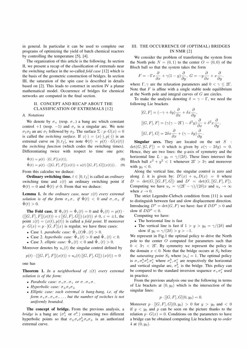
slow if y0 = γ/(2δ) > y > −1.We represent in Fig.1 the optimal policy to drive the Northpole to the center O computed for parameters such that0 < 3γ < 2Γ. By symmetry we represent the policy inthe domain x < 0. Note that the bridge occurs at S2 beforethe saturating point S3 where |us| = 1. The optimal policyis σ+σhs σ

b+σ

vs where σhs , σ

vs are respectively the horizontal

and vertical singular arc, σb+ is the bridge. This policy canbe compared to the standard inversion sequence σ+σvs usedin practice.

From the previous analysis one use the following in termsof Lie brackets at (0, y0) which is the intersection of thesingular lines:

p · [[G,F ], G](0, y0) = 0.

Moreover p · [[G,F ], G](0, y0) > 0 for y > y0 and < 0if y < y0 and p can be seen on the picture thanks to therelation p ·G(x) = 0. Conditions on the parameters to havea bridge can be obtained computing Lie brackets up to order4 at (0, y0).

x

y

L

ä

σ+ä

σ vs

ä

σ+

äσh

s

äσ+

äσ vs

N•

O•

• y0•S2 ••S3

•

Fig. 1. (left) Time optimal policy with a bridge compared with (right)inversion sequence.

IV. CONSTRUCTION OF A PLANAR(SYMMETRIC) MODEL

From the previous example we shall construct a localmodel (near (0, y0) in the previous example) which exhibitsthe previous behaviors.

A. Birth of the model.

We start with the following planar model:{x = uy = 1− εy2 where the singular arc σs is identified to

t 7→ (0, t) and corresponds to us(t) = 0. Such a line is fast ifε > 0 and slow if ε < 0. Moreover we have [G,F ] = 2xy ∂

∂y

and [[G,F ], G] = x ∂∂y . Hence singular trajectories are the

two lines: x = 0 and y = 0. By construction the verticalline can be followed by u = 0 and the horizontal line canbe followed by ”u =∞” so it cannot be tracked in practice.To construct the model one must bend this line and we getthe following.

B. The model

We consider the system

x = F (x) + uG(x), tf ← min|u|≤1

, x = (x, y) (10)

where F = (1−x2y) ∂∂y and G = −(y−1) ∂

∂x +x ∂∂y . Note

that integrating G led to circles centered at x = 0, y = 1.Computations. We have• [G,F ](x, y) = (−1 + x2y) ∂

∂x + (2xy(1− y) + x3) ∂∂y ,

• [[G,F ], G](x, y) = 2x(x2 − 2(y − 1)y

)∂∂x +(

x2(5− 8y) + 2y3 − 4y2 + 2y + 1)

∂∂y ,

• [[G,F ], F ](x, y) =(x2 − x4y

)∂∂x +

x(x4 + 4x2y2 − 6y + 2

)∂∂y ,

• det(G, [G,F ])(x, y) =x(x2(1− 2y) + 2y3 − 4y2 + 2y + 1

),

• D(x, y) = det(G, [[G,F ], G]) = −2x4 +x2(12y2 − 17y + 5

)− 2y4 + 6y3 − 6y2 + y + 1,

• D′(x, y) = det(G, [[G,F ], F ]) =x(x4 + x2

(−4y3 + 4y2 − 1

)+ 6y2 − 8y + 2

),

• Collinearity set: D′′(x, y) = 0 with D′′(x, y) =det(G,F ) = (y − 1)

(x2y − 1

).

Singular trajectories. The singular set is defined by Σs ={q, det(G, [G,F ])(q) = 0} and we have

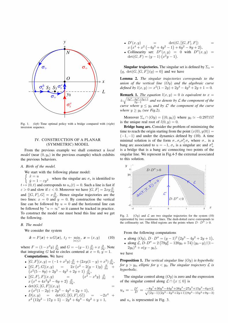
Lemma 2. The singular trajectories corresponds to theunion of the vertical line (Oy) and the algebraic curvedefined by l(x, y) := x2(1− 2y) + 2y3− 4y2 + 2y+ 1 = 0.

Remark 1. The equation l(x, y) = 0 is equivalent to x =

±√

2y3−4y2+2y+12y−1 and we denote by L the component of the

curve where y ≤ y0 and by L′ the component of the curvewhere y ≥ y0 (see Fig.2).

Moreover Σs ∩ (Oy) = {(0, y0)} where y0 ' −0.297157is the unique real root of l(0, y) = 0.

Bridge bang arc. Consider the problem of minimizing thetime to reach the origin starting from the point (x(0), y(0)) =(−1,−1) and under the dynamics defined by (10). A timeminimal solution is of the form σ−σsσ

b+σs where σ− is a

bang arc associated to u = −1, σs is a singular arc and σb+is a bridge that is a bang arc connecting two points of thesingular line. We represent in Fig.4-5 the extremal associatedto this solution.

D·D′′<0

D·D′′>0y0

L

L′

y

x

det(Y

, [Y,X

])=0

Fig. 2. (Oy) and L are two singular trajectories for the system (10)represented by two continuous lines. The dash-dotted curve corresponds tothe collinearity set. The filled regions are the points where D ·D′′ > 0.

From the following computations• along (Oy), D ·D′′ = (y − 1)2

(2y3 − 4y2 + 2y + 1

),

• along L, D·D′′ = 2(79y20 − 120y0 + 74

)(y0−y)/(1−

2y0)4 + o(y − y0),we have

Proposition 1. The vertical singular line (Oy) is hyperbolicfor y > y0, elliptic for y < y0. The singular trajectory L ishyperbolic.

The singular control along (Oy) is zero and the expressionof the singular control along L ∩ {x ≤ 0} is

us = −D′

D = −8y7+30y6−44y5+38y4−27y3+15y2−6y+2√(2y−1)(2y3−4y2+2y+1)(8y3−15y2+9y−3)

and us is represented in Fig. 3.

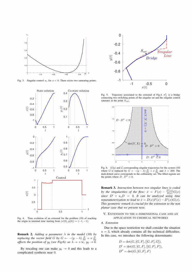
-1.0 -0.8 -0.6 -0.4

1.0

1.2

1.4

1.6

Fig. 3. Singular control us for x < 0. There exists two saturating points.

Fig. 4. Time evolution of an extremal for the problem (10) of reachingthe origin in minimal time starting from (x(0), y(0)) = (−1,−1).

Remark 2. Adding a parameter λ in the model (10) byreplacing the vector field G by G ← −(y − λ) ∂

∂x + x ∂∂y

affects the position of y0 (see Fig.6): as λ→ +∞, y0 → 0.

By rescaling one can make y0 → 0 and this leads to acomplicated synthesis near 0.

Fig. 5. Trajectory associated to the extremal of Fig.4. σb+ is a bridge

connecting two switching points of the singular set and the singular controlsaturates at the point Ssat.

det(Y,X) = 0

det(Y

,[Y,X

])=

0

L

D ·D′′ < 0

D ·D′′ < 0

D ·D′′ > 0

Fig. 6. (Oy) and L corresponding singular trajectories for the system (10)where G is replaced by G = −(y − λ) ∂

∂x+ x ∂

∂yand λ = 200. The

dash-dotted curve corresponds to the collinearity set. The filled regions arethe points where D ·D′′ > 0.

Remark 3. Interaction between two singular lines is codedby the singularities of the flow: x = F (x) − D′(x)

D(x) G(x)

since D′ + usD = 0. It can be analyzed using timereparameterization to lead to x = D(x)F (x)−D′(x)G(x).This geometric remark is crucial for the extension to the nonplanar case that we present next.

V. EXTENSION TO THE n-DIMENSIONAL CASE AND ANAPPLICATION TO CHEMICAL NETWORKS

A. Extension

Due to the space restriction we shall consider the situationn = 3, which already contains all the technical difficulties.In this case, we introduce the following determinants:

D = det(G, [G,F ], [[G,F ], G]),

D′ = det(G, [G,F ], [[G,F ], F ]),

D′′ = det(G, [G,F ], F )

and from (4)-(5)-(6) the singular control is given by

us(x) = −D′(x)

D(x).

We have three types of singular trajectories coming from thefold case classification:• hyperbolic: DD′′ > 0• elliptic: DD′′ < 0

and the so-called exceptional case corresponds to singulartrajectories such that H = p ·F (x) = 0. Eliminating p leadsto• exceptional: D′′ = 0.

Note that in this case the adjoint vector is either p or −p.Moreover using [3] the small time optimality status is:

time minimizing in the hyperbolic and exceptional case, timemaximizing in the elliptic case.

Again, since the singular trajectories are solutions of: x =

F (x) − D′(x)D(x) G(x) connections between singular arcs are

related to the behaviors of the solution of the reparameterizedequation:

x = D(x)F (x)−D′(x)G(x)

and in particular near the non isolated equilibria containedin D = D′ = 0.

This is the main issue for n ≥ 3 to analyze connectionsbetween singular arcs using a bridge in relation with theoccurrence of p(t) · [[G,F ], G](x(t)) = 0.

B. Application to chemical networks

We shall outline the discussion of the occurrence ofbridges for chemical networks, extending results from [5],[4]. The problem of maximizing the yield of one species[X] is converted into a minimizing the time to produce afixed [X] = d ([X] denoting the concentration of the speciesX).

One consider two reactions schemes:Case 1: A B Ck1 k2 : sequence of two irreversiblereactions ki = Ai exp(−Ei/(RT )), i = 1, 2, Ai, Ei areparameters, R is the gas constant and T is the temperature.

We introduce v = k1, x = log[A], y = [B], α = E2/E1,β = A2/A

α1 so that the dynamics takes the form: F =

−vx ∂∂x+(vx−βvαy) ∂∂y , G = ∂

∂v and the terminal manifoldis N = {[B] = y = d}. Computing one has• [G,F ] = x ∂

∂x + (−x+ αβvα−1y) ∂∂y ,

• [[G,F ], G] = (α(α− 1)βvα−2y ∂∂y ,

• [[G,F ], F ] = ((α− 1)βvαx ∂∂y ,

• D = det(G, [G,F ], [[G,F ], G]) = α(α− 1)βxyvα−2,• D′ = det(G, [G,F ], [[G,F ], F ]) = (α− 1)βx2vα,• D′′ = det(G, [G,F ], F ) = (α− 1)βxyvα.One wants to detect the existence of bridges near the ter-

minal manifold. In the discussion we introduce the followingstratification of N .• E : exceptional set: n ·F = 0 with n = (0, 1, 0) normal

to N and we get E : vx− βyvα = 0,• S : singular arcs so that n ·G = n · [G,F ] = 0, that is−x+ αβyvα−1 = 0.

ES

v = A1O

v

x

α < 1

O

x

v = A1

S

E

v

α > 1.

Fig. 7. Stratification of the manifold N .

We represent E and S on Fig.7 in the two cases α > 1 andα < 1.

Note that E forms the boundary of the terminal manifoldwhich can be reached from y(0) < d. In case α > 1, thereexists no admissible singular arcs and the optimal policy isu = +1. In the case α < 1, there exists hyperbolic singulararcs.Case 2: Consider now the following network where the

first reaction is reversible: A B Ck1 k2

k3

where ki =

Ai exp(−Ei/(RT )), i = 1, 2, 3. Denote v = k1, α =E2/E1, α′ = E3/E1, β = A2/A

α1 , β′ = A3/A

α1 , x

x = [A], [y] = [B] so that the dynamics is defined byF = (−vx + β′vα

′y) ∂∂x + (vx − β′vα

′y − βvαy) ∂∂y and

G = ∂∂v . One has

• [G,F ] = (x − α′β′vα′−1y) ∂∂x + (−x + α′β′vα

′−1y +αβvα−1) ∂∂y ,

• [[G,F ], G] = (−α′(α′ − 1)β′vα′−2y) ∂

∂x + (α′(α′ −1)β′vα

′−2y + α(α− 1)βvα−2) ∂∂y ,• D = det(G, [G,F ], [[G,F ], G]) = α(α−1)βxyvα−2 +α′β′αβ(α′ − α)vα+α

′−3y2

• D′ = det(G, [G,F ], [[G,F ], F ]) = y2(αβ2β′(α −

α′)v2α+α′−2 − α′ββ′2(α′ − α)vα+2α′−2 + β(αα′β′ −

αβ′)va+α′−1) + βxy(2α′β′ − 2αβ′)va+α

′−1 + (α −1)βx2vα

• D′′ = det(G, [G,F ], F ) = −βvαxy + (α′ −α)ββ′vα

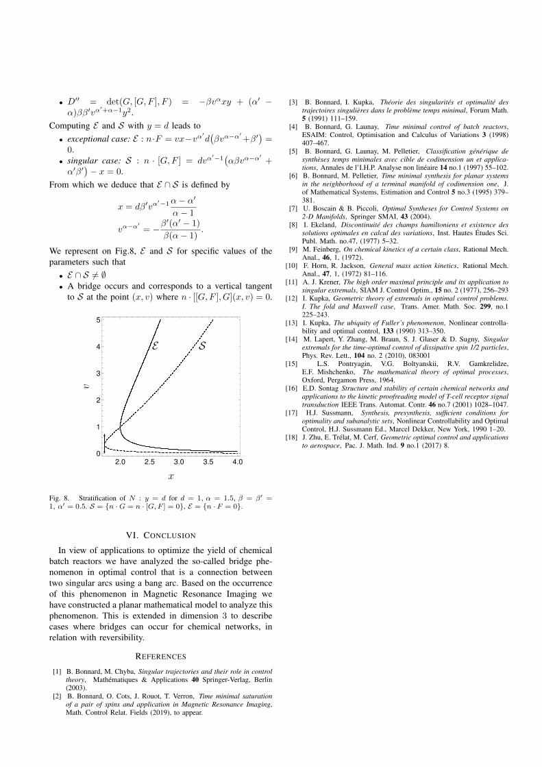
′+α−1y2.Computing E and S with y = d leads to• exceptional case: E : n·F = vx−vα′

d(βvα−α

′+β′

)=

0.• singular case: S : n · [G,F ] = dvα

′−1(αβvα−α′+

α′β′)− x = 0.

From which we deduce that E ∩ S is defined by

x = dβ′vα′−1α− α′

α− 1

vα−α′

= −β′(α′ − 1)

β(α− 1).

We represent on Fig.8, E and S for specific values of theparameters such that• E ∩ S 6= ∅• A bridge occurs and corresponds to a vertical tangent

to S at the point (x, v) where n · [[G,F ], G](x, v) = 0.

Fig. 8. Stratification of N : y = d for d = 1, α = 1.5, β = β′ =1, α′ = 0.5. S = {n ·G = n · [G,F ] = 0}, E = {n · F = 0}.

VI. CONCLUSION

In view of applications to optimize the yield of chemicalbatch reactors we have analyzed the so-called bridge phe-nomenon in optimal control that is a connection betweentwo singular arcs using a bang arc. Based on the occurrenceof this phenomenon in Magnetic Resonance Imaging wehave constructed a planar mathematical model to analyze thisphenomenon. This is extended in dimension 3 to describecases where bridges can occur for chemical networks, inrelation with reversibility.

REFERENCES

[1] B. Bonnard, M. Chyba, Singular trajectories and their role in controltheory, Mathematiques & Applications 40 Springer-Verlag, Berlin(2003).

[2] B. Bonnard, O. Cots, J. Rouot, T. Verron, Time minimal saturationof a pair of spins and application in Magnetic Resonance Imaging,Math. Control Relat. Fields (2019), to appear.

[3] B. Bonnard, I. Kupka, Theorie des singularites et optimalite destrajectoires singulieres dans le probleme temps minimal, Forum Math.5 (1991) 111–159.

[4] B. Bonnard, G. Launay, Time minimal control of batch reactors,ESAIM: Control, Optimisation and Calculus of Variations 3 (1998)407–467.

[5] B. Bonnard, G. Launay, M. Pelletier, Classification generique desyntheses temps minimales avec cible de codimension un et applica-tions, Annales de l’I.H.P. Analyse non lineaire 14 no.1 (1997) 55–102.

[6] B. Bonnard, M. Pelletier, Time minimal synthesis for planar systemsin the neighborhood of a terminal manifold of codimension one, J.of Mathematical Systems, Estimation and Control 5 no.3 (1995) 379–381.

[7] U. Boscain & B. Piccoli, Optimal Syntheses for Control Systems on2-D Manifolds, Springer SMAI, 43 (2004).

[8] I. Ekeland, Discontinuite des champs hamiltoniens et existence dessolutions optimales en calcul des variations, Inst. Hautes Etudes Sci.Publ. Math. no.47, (1977) 5–32.

[9] M. Feinberg, On chemical kinetics of a certain class, Rational Mech.Anal., 46, 1, (1972).

[10] F. Horn, R. Jackson, General mass action kinetics, Rational Mech.Anal., 47, 1, (1972) 81–116.

[11] A. J. Krener, The high order maximal principle and its application tosingular extremals, SIAM J. Control Optim., 15 no. 2 (1977), 256–293

[12] I. Kupka, Geometric theory of extremals in optimal control problems.I. The fold and Maxwell case, Trans. Amer. Math. Soc. 299, no.1225–243.

[13] I. Kupka, The ubiquity of Fuller’s phenomenon, Nonlinear controlla-bility and optimal control, 133 (1990) 313–350.

[14] M. Lapert, Y. Zhang, M. Braun, S. J. Glaser & D. Sugny, Singularextremals for the time-optimal control of dissipative spin 1/2 particles,Phys. Rev. Lett., 104 no. 2 (2010), 083001

[15] L.S. Pontryagin, V.G. Boltyanskii, R.V. Gamkrelidze,E.F. Mishchenko, The mathematical theory of optimal processes,Oxford, Pergamon Press, 1964.

[16] E.D. Sontag Structure and stability of certain chemical networks andapplications to the kinetic proofreading model of T-cell receptor signaltransduction IEEE Trans. Automat. Contr. 46 no.7 (2001) 1028–1047.

[17] H.J. Sussmann, Synthesis, presynthesis, sufficient conditions foroptimality and subanalytic sets, Nonlinear Controllability and OptimalControl, H.J. Sussmann Ed., Marcel Dekker, New York, 1990 1–20.

[18] J. Zhu, E. Trelat, M. Cerf, Geometric optimal control and applicationsto aerospace, Pac. J. Math. Ind. 9 no.1 (2017) 8.