congestion identification in a radio access transport …maguire/.c/degree-project... · congestion...
TRANSCRIPT

Degree project inCommunication Systems
Second level, 30.0 HECStockholm, Sweden
J A V I E R M O N T O J O V I L L A S A N T Aa n d
M A N U E L M A Q U E D A V I Ñ A S
Congestion Identification in a RadioAccess Transport Network
K T H I n f o r m a t i o n a n d
C o m m u n i c a t i o n T e c h n o l o g y

Congestion Identification in a Radio Access Transport
Network
Javier Montojo Villasanta &
Manuel Maqueda Viñas 2014-03-03
Master’s thesis
Examinor and academic adviser Professor Gerald Q. Maguire Jr.
School of Information and Communication Technology (ICT) KTH Royal Institute of Technology
Stockholm, Sweden


i
Abstract The convergence of mobile services and Internet has brought a radical change in mobile
networks. An all-IP network architecture, an evolution of the radio access transport network, is required to support new high-bandwidth services. Unfortunately, existing control mechanisms are insufficient to guarantee end users a high quality of experience. However, coordinating radio and transport network resources is expected to yield a more efficient solution.
This thesis project investigates the interactions between the congestion avoidance protocols, explicit congestion notification, and the traffic engineering metrics for latency and bandwidth, when using Open Shortest Path First with traffic engineering (OSPF-TE) as a routing protocol. Using knowledge of these interactions, it is possible to identify the appearance of bottlenecks and to control the congestion in the transport links within a radio access transport network.
Augmenting a topology map with the network’s current characteristics and reacting to evidence of potential congestion, further actions, such as handovers can be taken to ensure the users experience their expected quality of experience. The proposed method has been validated in a test bed. The results obtained from experiments and measurements in this test bed provide a clear picture of how the traffic flows in the network. Furthermore, the behavior of the network observed in these experiments, in terms of real-time performance and statistical analysis of metrics over a period of time, shows the efficiency of this proposed solution.
Keywords: Radio Access Transport Network, Open Shortest Path First – Traffic Engineering, Explicit Congestion Notification, Interface to the Router System, Congestion Identification


iii
Sammanfattning Tjänstekonvergensen av Internet- och mobila tjänster har medfört en radikal förändring i
mobilnäten. En ”All IP” nätverksarkitektur, en utveckling av radios transportnät. Utvecklingen krävs för att stödja de nya bredbandiga tjänsterna. Tyvärr är befintliga kontrollmekanismer otillräckliga för att garantera användarens kvalitetsupplevelse. Med att samordna radio- och transportnätverkets resurser förväntar man sig en effektivare lösning.
Detta examensarbete undersöker samspelet mellan protokoll för att undvika överlast, direkt indikation av överlast och trafikal statistik för fördröjning och bandbredd med trafikstyrning baserat på fördröjning och bandbredd , vid användning av Open Shortest Path First ( OSPF - TE ) som routingprotokoll. Med hjälp av information om dessa interaktioner, är det möjligt att identifiera uppkomsten av flaskhalsar och för att styra trafikstockningar i transportförbindelser inom ett radioaccess transportnät.
En utökad topologikarta med nätverkets aktuella egenskaper kommer att reagera på en potentiell överbelastning. Ytterligare åtgärder, till exempel överlämningar, vidtas i mobilnätet för att säkerställa användarens upplevda kvalitet. Den föreslagna metoden har validerats i en testmiljö. Resultaten från experiment och mätningar i denna testmiljö ger en tydlig bild av hur trafikflödena framskrider i nätverket. Beteendet hos nätverket som observeras i dessa experiment, i termer av realtidsprestanda och statistisk analys av mätvärden över en tidsperiod, visar effektiviteten av denna föreslagna lösning.
Nyckelord: Radio Access Transport Network, Open Shortest Path First – Traffic Engineering, Explicit Congestion Notification, Interface to the Router System, Congestion Identification

iv
Acknowledgements We would like to express our most sincere gratitude to all the people that have helped us
and supported us making possible this Master Thesis, namely:
Annikki Welin, our supervisor in Ericsson, for her constant support and project management, guiding us in a very didactic way, encouraging us always and proposing new ideas to open our minds, providing us the necessary equipment and a comfortable work space, resolving technical and organizational issues and introducing us people interested in the results of the projects and good contacts for our future. Summarizing, helping us in each aspect of the project.
Professor Gerald Q. Maguire Jr, our academic supervisor at KTH, for his indispensable feedback and continue brainstorm of ideas to improve our Thesis, guiding us when more we needed it and always with a teaching spirit in order to improve our apprenticeship.
Tomas Thyni, for helping us along the Thesis, providing interesting feedback and ideas, explaining deeply the most difficult concepts and motivating us to go further in our research.
To all our families and friends for their unconditional belief on us and encourage us to give our best for this project. Their advices and help, even in the distance, have been our main support during these months.

v
Table of contents
Abstract ........................................................................................... i Sammanfattning ............................................................................. iii Acknowledgements .......................................................................... iv
Table of contents ............................................................................. v
List of Figures ................................................................................. ix
List of Tables ................................................................................. xiii List of acronyms and abbreviations ................................................... xv
1 Introduction ............................................................................ 1 1.1 Overview ............................................................................. 1 1.2 Problem definition ................................................................. 3 1.3 Aim and goals ...................................................................... 4 1.4 Methodology ........................................................................ 4 1.5 Structure of the thesis ........................................................... 5
2 Background ............................................................................. 7 2.1 Evolution of the Radio Access Transport Networks ..................... 7
2.1.1 Evolved UTRAN ............................................................ 8 2.1.2 Evolved core network .................................................... 9 2.1.3 Radio Access Transport Network ................................... 10
2.2 Explicit Congestion Notification ............................................. 11 2.2.1 TCP support ............................................................... 12 2.2.2 Support from higher layers in a RAN ............................. 12
2.3 OSPF ................................................................................. 13 2.3.1 OSPF Functionality ...................................................... 14 2.3.2 Link State Advertisements (LSAs) ................................. 15 2.3.3 Opaque Link State Advertisement ................................. 16 2.3.4 OSPF Traffic Engineering ............................................. 17
2.4 Interface to the Routing System ........................................... 18 2.5 Potential sources of data for our measurements ...................... 19
2.5.1 TCP Extensions for High performance ............................ 19 2.5.2 Clock requirements and the NTP protocol ....................... 20 2.5.3 Simple Network Management Protocol (SNMP) ................ 20
2.6 Open source routing software ............................................... 21 2.6.1 Quagga router ............................................................ 21 2.6.2 OSPF API Extension .................................................... 23
2.7 Related work ...................................................................... 26
3 Design of a Congestion-Identification Mechanism ....................... 29 3.1 Overview of the Design ........................................................ 29 3.2 Real-Time Traffic Aware Router ............................................. 30
3.2.1 Measuring ................................................................. 31 3.2.1.1 Available Bandwidth ............................................. 31 3.2.1.2 Round-Trip Time and One-Way Delay ...................... 32

vi
3.2.1.3 Marked packets .................................................... 34 3.2.2 Monitoring & Policies ................................................... 34 3.2.3 Extended OSPF Router ................................................ 35
3.2.3.1 RTTA Sender ....................................................... 35 3.2.3.2 OSPF Router ........................................................ 37
3.2.4 RTTA Router Summary ................................................ 37 3.3 Real-Time Traffic Aware Receiver .......................................... 37
3.3.1 Collecting of information module ................................... 38 3.3.2 Analysis and Visualization module ................................. 38
3.4 Summary of the design ........................................................ 39
4 Congestion–Identification Implementation ................................. 41 4.1 Set up of the Environment ................................................... 41 4.2 Real-Time Traffic Aware Router ............................................. 43
4.2.1 Measuring module ...................................................... 44 4.2.1.1 Available Bandwidth ............................................. 45 4.2.1.2 Round-Trip Time and One-Way Delay ...................... 45 4.2.1.3 Marked packets .................................................... 46
4.2.2 Monitoring & Policies modules ...................................... 47 4.2.3 Extended OSPF Router module ..................................... 48
4.2.3.1 RTTA Sender ....................................................... 48 4.2.3.2 Quagga OSPF API ................................................. 49 4.2.3.3 OSPF Router ........................................................ 49
4.3 Real-Time Traffic Aware Receiver .......................................... 49 4.3.1 Collecting of information module ................................... 50
4.3.1.1 OSPF-TE Receiver ................................................. 50 4.3.1.2 CE detection ........................................................ 51
4.3.2 Analysis and Visualization module ................................. 51 4.3.2.1 Real-Time Visualization sub-module ........................ 52 4.3.2.2 Time-Capture Analysis sub-module ......................... 54
4.4 Conclusion of this implementation chapter .............................. 55
5 Verification of the results ........................................................ 57 5.1 Congestion Emulation Tools .................................................. 57 5.2 Description of the different scenarios ..................................... 58
5.2.1 Scenario A: Congestion-less network ............................. 60 5.2.2 Scenario B: Congested path in the network .................... 60
5.3 Analysis of the results ......................................................... 61 5.3.1 Real Time Visualization ................................................ 61
5.3.1.1 Per Router Interface Analysis ................................. 63 5.3.1.2 Per Path Analysis ................................................. 65
5.3.2 Time-Capture Analysis ................................................ 67 5.3.2.1 Per Router Interface Analysis ................................. 68 5.3.2.2 Per Path Analysis ................................................. 70
5.4 Conclusion of the Verification of the Results ............................ 72
6 Conclusions and Future work ................................................... 73 6.1 Conclusions ........................................................................ 73 6.2 Future work ....................................................................... 74 6.3 Required reflections ............................................................ 75

vii
Bibliography .................................................................................. 77
Appendix A Analysis and Visualization: Implementation .................... 83
Appendix B Analysis and Visualization: Verification for both scenarios . 89


ix
List of Figures Figure 1-1: Relationship between the Radio Access Transport Network and the
eNodeBs. .......................................................................................................... 2 Figure 2-1: LTE network architecture. ................................................................................ 8 Figure 2-2: The protocol stack of the S1 interface in a LTE network. ............................... 9 Figure 2-3: ECN field in the TCP header .......................................................................... 12 Figure 2-4: OSPF Packet Header [17] ............................................................................... 15 Figure 2-5: Common LSA Header[17] ............................................................................. 15 Figure 2-6: Options Field [21] .......................................................................................... 16 Figure 2-7: Opaque LSA Header Format [21] .................................................................. 16 Figure 2-8: TE-LSA header format and TLV [23] ............................................................ 17 Figure 2-9: I2RS model ..................................................................................................... 19 Figure 2-10: TCP Timestamp Header Field ........................................................................ 20 Figure 2-11: Quagga Router Architecture ........................................................................... 22 Figure 2-12: Quagga OSPF Daemon Architecture ............................................................. 23 Figure 2-13: The OSPF API Protocol phases[46] ............................................................... 25 Figure 3-1: Congestion-Identification scenario ................................................................ 29 Figure 3-2: Architecture of the Real-Time Traffic Aware Router .................................... 31 Figure 3-3: Sequence of messages between two routers, R1 and R2, for measuring
RTT and one-way delay, based on sharing router timestamps ...................... 33 Figure 3-4: LSA-Opaque Packet ....................................................................................... 35 Figure 3-5: Three alternative Sub-TLVs proposals .......................................................... 36 Figure 3-6: Architecture of the Real-Time Traffic Aware Receiver ................................. 38 Figure 4-1: Test bed Deployment ..................................................................................... 41 Figure 4-2: RTTA Router Flowchart ................................................................................ 44 Figure 4-3: RTTA Receiver Flowchart ............................................................................. 50 Figure 4-4: Real-Time Visualization Capture ................................................................... 52 Figure 4-5: Example of Real-Time Visualization for RTT and Available Bandwidth
by interface ..................................................................................................... 53 Figure 4-6: Example of Real-Time Visualization for RTT and Available Bandwidth
by path ............................................................................................................ 53 Figure 4-7: Example of Real-Time Visualization for CE packets .................................... 54 Figure 4-8: Time-Capture Visualization of the interfaces of the RTTA Router of the
VM-32 ............................................................................................................ 55 Figure 5-1: Scenario A ...................................................................................................... 59 Figure 5-2: Scenario B ...................................................................................................... 61 Figure 5-3: Video seen by a UE connected to eN2 ........................................................... 62 Figure 5-4: Video seen by a UE connected to eN1 ........................................................... 62 Figure 5-5: Real Time Visualization of the RTT by Interfaces in Scenario A ................. 63 Figure 5-6: Real Time Visualization of the RTT by Interfaces in Scenario B ................. 63

x
Figure 5-7: Real Time Visualization of the Available Bandwidth by Interfaces in Scenario A ...................................................................................................... 64
Figure 5-8: Real Time Visualization of the Available Bandwidth by Interfaces in Scenario B ...................................................................................................... 64
Figure 5-9: Real Time Visualization of the average number of packets marked per Interface in Scenario B ................................................................................... 64
Figure 5-10: Real Time Visualization of the average number of CE marked packets detected at eN1 ............................................................................................... 65
Figure 5-11: Real Time Visualization of the RTT by Paths in the Scenario A .................. 66 Figure 5-12: Real Time Visualization of the RTT by Paths in the Scenario B ................... 66 Figure 5-13: Real Time Visualization of the Available Bandwidth by Path in Scenario
A ..................................................................................................................... 67 Figure 5-14: Real Time Visualization of the Available Bandwidth by Path in Scenario
B ..................................................................................................................... 67 Figure 5-15: Time Capture Analysis of the RTT by Interfaces in Scenario A ................... 68 Figure 5-16: Time Capture Analysis of the RTT by Interfaces in Scenario B ................... 68 Figure 5-17: Time Capture Analysis of the Available Bandwidth by Interfaces in
Scenario A ...................................................................................................... 69 Figure 5-18: Time Capture Analysis of the Available Bandwidth by Interfaces in
Scenario B ...................................................................................................... 69 Figure 5-19: Time Capture Analysis of the Average Number of Marked Packets by
Interface in Scenario B ................................................................................... 69 Figure 5-20: Time Capture Analysis of the RTT by Path in Scenario A ............................... 70 Figure 5-21: Time Capture Analysis of the RTT by Path in Scenario B ............................... 70 Figure 5-22: Time Capture Analysis of the Available Bandwidth by Paths in the
Scenario B ...................................................................................................... 71 Figure 5-23: Time Capture Analysis of the Average of Number Marked Packets and CE
Detected by Path in Scenario B ...................................................................... 71 Figure 6-1: Capture of the Real-Time Visualization in a certain moment. ........................... 85 Figure 6-3: 90
Appendix Figure A-1: Capture of the Real-Time Visualization in a certain moment. .......... 85 Appendix Figure A-2: Time-Capture Analysis for the interfaces of the Router .22 in 60
minutes. .......................................................................................................... 86 Appendix Figure A-3: Time-Capture Analysis for two paths of the test-bed in 60
minutes. .......................................................................................................... 87 Appendix Figure B-1: Capture of the Real-Time Visualization of the Scenario A in a
certain moment. .............................................................................................. 90 Appendix Figure B-2: Time-Capture Analysis for the Router B in the scenario A in 60
minutes. .......................................................................................................... 91 Appendix Figure B-3: Time-Capture Analysis of the scenario B for paths in 60 minutes. ... 92 Appendix Figure B-4: Capture of Real-Time Visualization for the scenario B in a
certain moment. .............................................................................................. 93

xi
Appendix Figure B-5: Time-Capture Analysis for the Router B for the scenario B in 60 minutes. .......................................................................................................... 94
Appendix Figure B-6: Time-Capture Analysis for the scenario B for paths in 60 minutes. .......................................................................................................... 95


xiii
List of Tables Table 2-1: ECN field in the IP header ............................................................................. 11 Table 2-2: OSPF Message Types [17] ............................................................................. 14 Table 2-3: Opaque Link-State Advertisements (LSA) Option Types [22] ...................... 16 Table 2-4: Top Level Types in TE LSAs [28] ................................................................. 17 Table 2-5: Sub-TLVs types of a Node Attribute TLV[32] .............................................. 18 Table 3-1: Timestamp Equations ..................................................................................... 33 Table 4-1: Configuration of each of the computers used to realize the test-bed ............. 43 Table 4-2: Sqlite Database Contents ................................................................................ 48 Table 5-1: Tools used for Congestion Emulation and Simulation ................................... 57 Table 5-2: RED queues configuration ............................................................................. 58 Table 5-3: RTTA Router policies configuration .............................................................. 58 Table 5-4: VLC streaming configuration ......................................................................... 59


xv
List of acronyms and abbreviations
2G Second Generation
3G Third Generation
3GPP Third Generation Partnership Project
4G Fourth Generation
ABR Area Border Router
ACK acknowledgement
API Application Programming Interface
AQM Active Queue Management
AS Autonomous System
ASBR Autonomous System Boundary Router
BGP Border Gateway Protocol
CE Congestion Evidence
CLI Command Line Interface
CWR Congestion Window Reduced
ECE ECN-Echo
ECN Explicit Congestion Notification
EIGRP Enhanced Interior Gateway Routing Protocol
eNB Evolved NodeB
eUTRAN Evolved UTRAN
FIB Forwarding Information Base
GPRS General Packet Radio Service
GSM Global System Mobile
GTP GPRS Tunneling Protocol
HSS Home Subscriber Server
I2RS Interface To the Routing System
IANA Internet Assigned Numbers Authority
iBGP internal Border Gateway Protocol

xvi
IETF Internet Engineering Task Force
IGP Interior Gateway Protocol
IGRP Interior Gateway Routing Protocol
IPv4/6 Internet Protocol version 4/6
IS-IS Intermediate System to Intermediate System
ITU International Telecommunication Union
LSA Link-State Advertisements
LSDB Link-State Database
LSU Link-State Update
LTE Long Term Evolution
Mbps Megabits per second
MIB Management Information Base
MIMO Multiple Input Multiple Output
MME Mobility Management Entity
NAS Non-Access-Stratum
NAT Network Address Translation
NTP Network Time Protocol
NSSA Not-So-Stubby-Area
OID Object Identifier
OFDM Orthogonal Frequency Division Multiplexing
OS Operating System
OSPF Open Shortest Path First
OSPF-TE OSPF with TE extensions
OSR Open Source Routing
PDN-GW Packet Data Network Gateway
PTP Precision Time Protocol
QoE Quality of Experience
QoS Quality of Server
RAN Radio Access Network
RATN Radio Access Transport Network

xvii
RED Random Early Detection
RFC Request For Comments
RIB Routing Information Base
RIP Routing Information Protocol
RRM Radio Resource Manager
RTTA Real-Time Traffic Aware
RTT Round Trip Time
S-GW Serving Gateway
S1-AP S1- Application Protocol
SC-FDM Single-Carrier Frequency Division Multiplexing
SCTP Stream Control Transmission Protocol
SNMP Simple Network Management Protocol
SON Self-organizing Network
SPF Shortest Path First
TCP Transport Control Protocol
TE Traffic Engineering
TED Traffic Engineering Database
TLV Type/Length/Value
UE User Equipment
UMTS Universal Mobile Telecommunicaitons System
UTRAN UMTS Terrestrial Radio Access Network
WAN Wide Area Network


1
1 Introduction This chapter provides an introduction to the subject of this master’s thesis project in order
to help readers understand the scope of this project. Next, the problems addressed in this thesis project are described, followed by a statement of the project’s aim and goals. The research methodology is described. The chapter concludes with an overview of the structure of this thesis.
1.1 Overview The convergence of mobile services and Internet has brought about a radical change in
mobile networks. The number of mobile broadband subscribers continues to grow at a tremendous rate. The number of active mobile subscriptions is over 2096 million according to International Telecommunication Union (ITU) statistics [1]. Cisco expects that the number of subscribers will be four times as large in four years. This is due to the radical increase in the number of devices and the number of mobile subscribers, with 3.4 billion Internet users expected in 2016 [2]. Along with this growth in the number of mobile subscribers there has been a substantial increase in mobile traffic. Some examples that illustrate this include Ericsson’s prediction of a 10-fold increase in mobile traffic by 2016 as compared to 2011 [3] and studies by Cisco who expects an increase in the global mobile Internet data traffic of 10.8 Exabytes (i.e., 10.8 x 1018 bytes) per month by 2016 [2]. These expectations of growth do not stop and it is very likely that in the next decade the rate of growth will continue to increase. As the traffic demand due to mobile data applications continues to grow dramatically, mobile operators are investing heavily in infrastructure upgrades to support the network demands of their subscribers [4].
In order to organize and coordinate the evolution of mobile networks the 3rd Generation Partnership Project (3GPP) was created in 1998 to lead and produce technical specifications and technical reports for a third generation (3G) Mobile System based on evolved second generation (2G) Global System for Mobile Communication (GSM) core networks and the radio access technologies that they support[5]. A new generation of mobile networks, 3GPP’s Long Term Evolution (LTE), is being rapidly deployed by mobile operators as they try to satisfy their subscriber’s demands. By September 2013, nearly 100 cities around the globe had started commercial deployment of LTE systems [6].
LTE is a fourth generation (4G) wireless broadband technology * . LTE provides significantly increased peak data rates in comparison with 3G Universal Mobile Telecommunication Systems (UMTS), with the potential for 100 Mbps downstream and 30 Mbps upstream, reduced latency, scalable bandwidth capacity, and backwards compatibility with existing GSM and UMTS technology. Future developments are expected to yield peak throughput on the order of 300 Mbps [7].
The upper layers of the LTE protocol stack are based on many different protocols, but the IP protocol is fundamental to this protocol stack resulting in an all-IP network similar to the current state of wired communications. LTE supports mixed data, voice, video, and messaging traffic to and from user equipment (UE). Today, the radio base stations (called eNodeBs) are connected via IP technology to the core network, thorough a network of routers forming a so-called Radio Access Transport Network. This network is connected via Serving * More correctly, LTE-Advanced is a 4G system according to the ITU-T criteria for 4G systems.

2
Gatewaturn is architec
Figure 1
Howdemandthe incrrates; thand mo(QoE) [
Ideafairnessother suEach usservicesthere isservice willing best sercurrent
ays (S-GWsconnected
cture is show
1-1: Rela
wever, evends for capacreasing numhe appropriaore relevan[8].
ally the netws we shouldubscribers eser’s traffic s with the as congestion
providers to pay for
rvice possibneeds of th
s) to one ord with thewn Figure 1
ationship be
n the advancity and incmber of botate manage
nt in order
work should not allowexperience p
has to be pappropriate n. As in maseek to pr- no more,
ble with the he subscribe
r more pack Internet a
1-1.
etween the R
nces alreadycreased datath human ument and c
to ensure
d be accessw some userpoor qualityprioritized su
bandwidthany other movide theirno less - aresources trs.
ket data netand other
Radio Access
y offered bya throughpuusers and deontrol of al
e subscriber
sible and fars to load thy of service uch that the
h and withinmarkets, mor subscriberand that is wthat have be
twork gatewpacket ne
s Transport
y LTE are uut. Due to thevices, and ll this amours of a rel
air to all thehe Radio A(QoS) or c
e network an the desire
obile broadbrs with exawhy our effeen deploye
ways (PDN-tworks. Th
Network an
unable to hhe growth ithe increas
unt of trafficliable Qual
e users. In oAccess Netwannot even llows all ofed latency bband and fixactly what forts are dired in order t
-GWs), whihis overall
nd the eNod
handle the ein number osing aggregc is becominlity of Exp
order to enswork (RANaccess the
f the users tbounds, evexed line brothey need
rected to ento satisfy th
ich is in system
deBs.
expected of users, gate data ng more perience
sure this N), while
internet. o access en when oadband and are
nsure the he actual

3
The expectations described above explain why an all-IP network architecture, an evolution of the radio access transport network, is required to support the current and future high-bandwidth services. Unfortunately, the existing control mechanisms are insufficient to guarantee end users a high QoE.
Earlier studies focused on different solutions to address congestion in the transport and radio access networks. However, in this thesis project a more efficient solution is proposed based upon coordinating the radio and transport access networks.
1.2 Problem definition The evolution of mobile networks towards new high-bandwidth services brings new
challenges due to the mobile network’s behavior. The number of IP applications is increasing and the applications are creating new requirements for mobile networks. Mobile network operators need to ensure QoE and equitable services for all of their subscriber [8]. In order to meet this goal the mobile network operators need to skillfully manage their network resources. In order to do this management the network operator needs to have as much information as possible about the network’s current status and the expected demands upon their network.
In particular, the RATN equipment that was designed to provide UEs with access to the Internet and other packet data networks needs new mechanisms to meet the requirements of 4G networks. Providing adequate capacity is one of the main problems to solve for existing networks, especially providing adequate capacity in the aggregation network structure and the last hop (the wireless link between the UE and the base station) – as these are typically where bottlenecks appear[10]. Bandwidth bottlenecks can have a large negative impact on the user’s perceived QoE, hence avoiding such bottlenecks forming becomes an important challenge for the mobile networks operators. For this reason, the existence and evolution of congestion avoidance and control mechanisms is crucial in such networks.
Unfortunately, the existing congestion mechanisms, such those employed in the transmission control protocol (TCP) or Explicit Congestion Notification (ECN), are only handled by the endpoints of the communication, leaving the networks in between with no part in this task (other than marking packets in order to provide ECN). Today nodes along the path between the UE and the PDN-GW generally deal with congestion imply by deciding which packets to drop. Moreover, the congestion information received at the endpoints is very limited, typically the endpoints only knowing the presence of congestion along a communication path, but do not have any details about which part of the network is congested nor what the network’s state is along the path. As a result the endpoints cannot initiate actions to systematically deal with this congestion. Hence the network must collect and utilize information to deal with this congestion. Today reports of congestion in real-time are becoming necessary with a radio access transport network in order to avoid bottlenecks forming. For example, this information can be forwarded to a radio resource manager (RMM) or Mobility Management Entity (MME) for further action (e.g. dropping some UEs’ connections or initiating a handover for one or more UEs).

4
For all of the reasons described above, new congestion identification mechanisms are needed and there needs to be a way to propagate information about congestion to the relevant entities within the networks and in some cases to the relevant endpoints. The relevant network entities are the RRMs, MMEs, PDN-GWs, eNodeBs, and the routers in the radio access transport network*. For this reason, this master’s thesis project studies the interaction between congestion avoidance protocols (such as ECN) and traffic engineering (specifically Open Shortest Path First Traffic Engineering - OSPF-TE) in a radio access transport network in order to meet current and near future requirements.
1.3 Aim and goals The aim of this master’s thesis project is to provide Ericsson, the company in which this
project is being conducted, with the basis for a mechanism to identify congestion in a radio access transport network. This is one of the challenges which the company is currently facing as part of their tremendous effort to offer solutions that can better adapted to the growth in the amount of mobile broadband traffic.
Given this aim, the goal of this thesis project can be split into two parts. The first part is to investigate protocols related to congestion control and the interactions between these protocols. The second part is to propose a mechanism that identifies congestion in a radio access transport network. The following specific sub-goals will guide us throughout the project to achieve the aim and goals proposed above:
• Study the ECN protocol and the OSPF-TE metrics for delay and bandwidth.
• Investigate ways to implement them in a radio access transport network of a LTE network.
• Investigate their interaction in order to gain enhanced knowledge of congestion, in order to be able to identify congestion in the radio access transport network.
• Propose a mechanism based upon the results of the investigation and integrate this mechanism in a test bed, based on Quagga (routing software) routers, that simulates the proposed solution for evaluation in a test scenario.
1.4 Methodology To carry out and accomplish the objectives of this project, qualitative and quantitative
methods will be used. The first parts of this master’s thesis project are based on a qualitative research methodology and then, with the information collected from the test bed deployment of our scenario, initiate a quantitative study. The schedule and problems encountered in this thesis project can be described as the following three steps:
• Background study and design proposal: At the beginning of our project, our main task was to obtain the relevant knowledge required to understand and carry out this master’s thesis project. In order to accomplish this part, we started with a literature and studied related work. The background study considered the three main prerequisites of our thesis. First of all we needed to have a wide overview of the new System Architecture Evolution (SAE), especially as LTE. While we reading the literature for this part, we mainly focused on the RAN. After this, we studied OSPF-TE and ECN, as these were the main protocols that we expected to use. The goals of this sub phase were: (1) to understand OSPF and OSPF-TE behavior along with
* For readers familiar with existing GSM and UMTS networks, the radio access transport network replaces the
so-called “back-haul” network with an IP based network as part of the transformation to an all-IP network.

5
its LSA types and the architecture of Opaque LSAs, and all the functionality of ECN protocol; (2) identify relevant processing metrics and virtualization information that OSPF-TE Opaque LSAs would need to convey and how these can interact with ECN; and (3) investigate how OSPF-TE and ECN can be extended and implemented in our transport network scenario. Finally with all the information gathered, we have proposed a design of a mechanism for achieving our goals.
• Test-bed implementation: This step involves the deployment of a test-bed and the use of this test bed with a test scenario to implement and evaluate a proposed solution for the congestion identification problem. This step took the largest amount of time during this thesis project. Part of the reason for this was the time needed for the development and study of a suitable scenario and for the implementation of the solution that we propose. Initially, we implemented all the extensions and developments that our test-bed would need to run OSPF-TE and ECN. After this, the experiments with our test bed started and we begin to obtain and collect the information necessary to identify the congestion.
• Verification: The final part of this project has been divided in two different steps. First a complete evaluation of the designed network and elements has been done. This step has appraised the functioning of the mechanism implemented; observing that the information about congestion identification collected is accessible for the nodes in the network. The second step formulates an analysis of different simulations of our test bed, in order to test the interaction between the evidence of congestion identified with ECN and the congestion information provided by the nodes through OSPF-TE. With visualization and monitoring of the information obtained, this interaction is verified.
1.5 Structure of the thesis The chapter one is the introduction to the problem, aim, goals, and methodology. The
motivation for the fulfillment of this project and the main objectives of it are explained.
The second chapter provides the background and the knowledge that a reader initiated in the mobile network subject needs to fully understands the rest of this thesis. This chapter gives and introduction to the evolution of the RAN and explains OSPF-TE and other mechanisms and protocols. It ends with an introduction to the routing software used
Chapter three describes the method that will be used to achieve the goals described above. The whole explain of the design of the network and its elements. Different options and methods have been taken into account and are discussed in this chapter
The fourth chapter explains in detail the implementation of the design explained in the previous chapter. This chapter takes into consideration the limitations of our test bed, explains them and its alternatives and finally discusses how these have influenced in the final solution.
The chapter five makes a complete analysis of the solution set out. A whole overview of the obtained information is given, followed with a study of certain simulated scenarios that corroborate this solution proposed.
The final chapter six states the conclusions reached during this project. Together with these conclusions a suggestion of the possible future works and a reflection of the consequences of this master thesis is considerate it.


7
2 Background This chapter begins by introducing the reader to the evolution of radio access transport
networks in order that the reader can understand the context of this project. After this, a brief introduction is given to the Internet Engineering Task Force (IETF) proposed Interface to the Routing System. The Explicit Congestion Protocol is explained, followed by an introduction to OSPF-TE. This chapter continues with an explanation of a wide set of protocols and techniques needed for a better understanding of the measurements, implementation, and design that will be presented in subsequent chapters. Section 2.6 presents the Quagga router and the OSPF API, as they will be used to implement the proposed solution that will subsequently be evaluated in a test bed. The final section of the chapter surveys related work.
2.1 Evolution of the Radio Access Transport Networks Since GPRS first enabled user applications to easily send data packets over mobile
networks, the use of packet based communication technology in wide area cellular mobile networks has experienced a rapid evolution to today’s mobile broadband internet as experienced by increasing numbers of subscribers. 3GPP is responsible for evolving the GSM, UMTS, and LTE standards. This section summarizes the aspects of these networks that are needed to understand the context of the thesis.
Both, UMTS and LTE, introduced a redesign of the Terrestrial Radio Access Network (TRAN), referred to as UTRAN and Evolved-UTRAN (eUTRAN) respectively. UMTS combined properties of the earlier circuit-switched voice networks with properties of packet-switched data networks in order to support new services. Despite the improvements brought by UMTS, it has been limited by several of its design decisions in the same way as its predecessors were. LTE is an evolution of UMTS in which both the radio and core networks were redesigned. The main LTE improvements over UMTS are Orthogonal Frequency-Division Multiplexing (OFDM) with Multiple Input Multiple Output (MIMO) support for transmitting the data over the air interface and an all-IP approach to simplify the design and implementation of the air interface, radio network, and core network [11]. In this thesis we will focus on the later improvement, specifically we focus on how the network architecture has evolved and, in particular, how the radio and core networks are implemented in this new architecture.
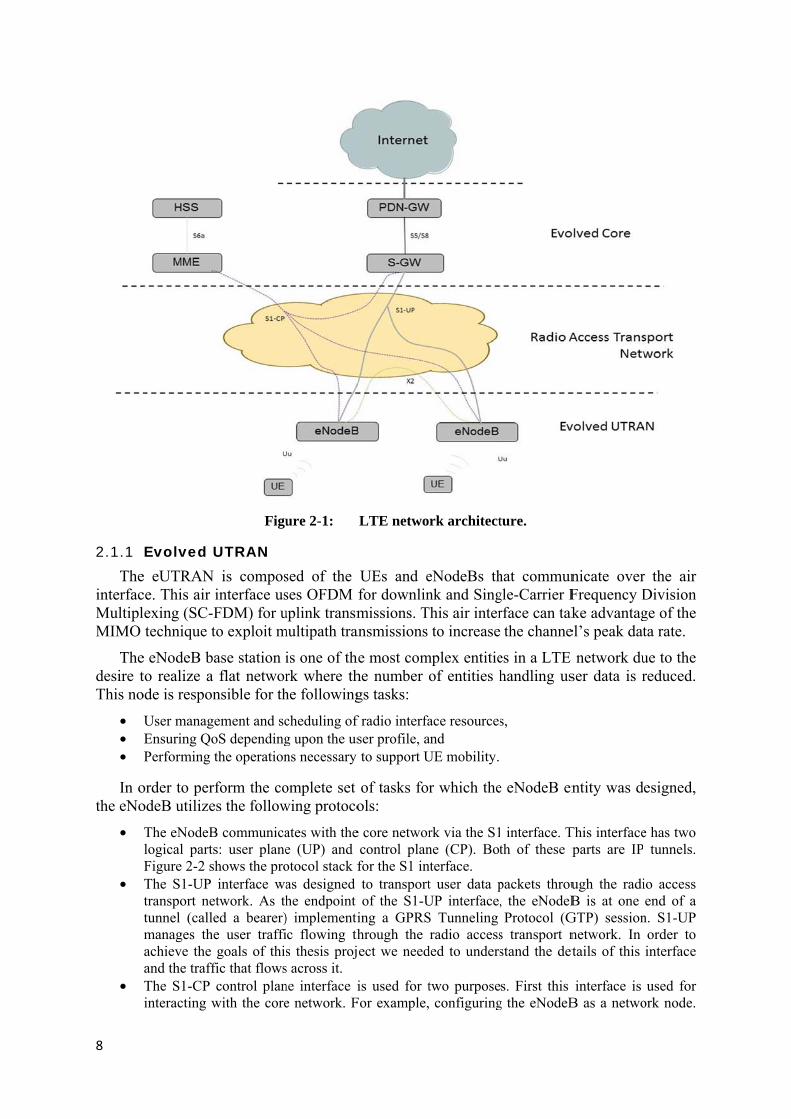
The LTE network architecture is divided in to a radio network (referred to as eUTRAN) and a core network (referred to as the Evolved Packet Core). This architecture is shown in Figure 2-1. According with Olsson, et al. [7], two main principles have guide the design of this architecture: a flat architecture, as few nodes as possible handle the user data traffic, and a separation of control data from user data.
8
2.1.1
TheinterfacMultiplMIMO
Thedesire tThis no
• • •
In othe eNo
•
•
•
Evolved Ue eUTRAN ce. This air lexing (SC-Ftechnique t
e eNodeB bato realize a ode is respon
User manageEnsuring QoPerforming t
order to perodeB utilizeThe eNodeBlogical partsFigure 2-2 sThe S1-UP transport netunnel (callemanages theachieve the and the traffThe S1-CP interacting w
Figu
UTRAN is compos
interface usFDM) for uto exploit m
ase station iflat networ
nsible for th
ement and scoS dependingthe operation
form the coes the followB communicas: user planehows the prointerface wa
etwork. As thed a bearer)e user traffigoals of thi
fic that flowscontrol plan
with the core
ure 2-1:
sed of the ses OFDM uplink transm
multipath tra
is one of thrk where thhe following
cheduling of g upon the usns necessary
omplete set wing protocoates with thee (UP) and otocol stack fas designed he endpoint ) implementiic flowing ths thesis projs across it. ne interface ie network. F
LTE netwo
UEs and efor downlinmissions. T
ansmissions
he most comhe number gs tasks:
f radio interfaser profile, ato support U
of tasks forols:
e core networcontrol planfor the S1 into transportof the S1-U
ing a GPRShrough the ect we need
is used for tFor example,
rk architect
eNodeBs thnk and Sing
This air interto increase
mplex entitieof entities h
ace resourcesand UE mobility.
r which the
rk via the S1ne (CP). Botnterface. t user data pUP interface,S Tunneling radio access
ded to unders
two purpose configuring
ture.
hat commungle-Carrier Frface can takthe channe
es in a LTE handling us
s,
e eNodeB en
interface. Tth of these p
packets throu, the eNodeBProtocol (G
s transport nstand the det
s. First this g the eNodeB
nicate overFrequency Dke advantag
el’s peak dat
network duser data is r
ntity was d
This interfaceparts are IP
ugh the radiB is at one
GTP) sessionnetwork. In tails of this
interface is B as a netwo
r the air Division ge of the ta rate.
ue to the reduced.
esigned,
e has two tunnels.
io access end of a
n. S1-UP order to interface
used for ork node.

9
Second, this interface is used for signaling messages that concern the users of the system, such as signaling for establishing a tunnel between the eNodeB and SG-GW, for maintaining a user service, or for perform handovers as directed by the MME.
• The X2 interface enables one eNodeB to communicate directly with other eNodeBs. This eNodeB enables a handover between two eNodeBs to be performed without involving the core network. Such a handover can only be performed if the target eNodeB is known and reachable through the identification of this eNodeB made by the UE.
The eNodeBs communicate through the transport network using the S1-UP, S1-CP, and X2 interfaces to entities connected to the evolved core network.
S1
User Plane Control Plane
Applications
IP NAS
GTP-U S1-AP
UDP SCTP
IP
L2
L1
Figure 2-2: The protocol stack of the S1 interface in a LTE network.
In addition, self-optimizing and self-organizing network (SON) functions has been introduced in LTE networks that leverages network intelligence based on measurements performed by the eNodeB in order to automate the configuration and optimization of the Radio Access Network. Some of the use cases of SON functions are[12]: • Automatic Neighbor Relation (ANR), enabling automatic configuration of neighbor cells. • Load balancing: adjustment of cell handover parameters to balance the traffic between cells. • Handover: optimizing the mobility functionalities as identification and avoidance of Ping-
Pong behavior or decrease the number of handovers. • Network monitoring.
2.1.2 Evolved core network The evolved core network includes MMEs, S-GWs, PDN-GWs, and the Home Subscriber
Server (HSS).
A MME is responsible for all the signaling messages between a UE and the core network and between the eNodeBs and the core network. The MME performs the following tasks [11]:

10
• Helping in the exchange of authentication information between a UE and the HSS. • Establishing a tunnel (bearer) for user data packets between an eNodeB and a S-GW. • Handover support when no X2 interface is available and modifying the tunnels after a
successful handover. • Manage idle mode UEs when the UE has released its air interface connection and released its
resources in the radio network.
In addition to the use of the interfaces described above, the MME uses the interfaces S1-CP and S6a to communicate with the others entities of the core network, as shown in Figure 2-1.
The S-GW manages the user data packets by acting as a bridge between the radio network, where the S1-UP GTP tunnels terminate, and the core network, where an end of the S5-UP GTP tunnel is situated. The S1 and S5 tunnels, for a UE, are independent of each other and can be separately modified as required. If there is a handover where the UE changes from one eNodeB to other eNodeB managed by the same MME, then only the S1-UP GTP tunnel is modified.
The PDN-GW is a gateway to the Internet or other packet data networks. Here, the user data packets from an external network are encapsulated in a S5-GTP tunnel and forwarded to the S-GW which is currently responsible for this UE. The PDN-GW is responsible for assigning IP addresses after a UE is authenticated via the MME’s communication with the HSS. The PDN-GW can utilize network address translation (NAT) to map many internal IP addresses to a smaller number of public IP; enabling many IP tunnels to connect to one UE.
The HSS stores all the subscriber related information. This includes credentials for authentication and access authorization. The MME requests subscription-related data via messages to the HSS over the S6a interface.
2.1.3 Radio Access Transport Network As it is shown it the Figure 2-1, the radio access transport network is situated between the
eUTRAN and the Evolved Core carrying out the communications between both parts of the network. It can be divided in an access part, from the eNodeBs to concentration points, and an aggregation part, to transport mobile flows from concentration points to the core network. Both parts are composed of different technologies: microwave, copper cables or optical fiber (GPON), depending of the available resources in the concerned area and bandwidth requirements. The routers, located in each node of the Radio Access Transport Network, are the responsible of forwarding packets through the network from the access to the aggregation part. Although, none difference is conceived in the routing and the forwarding between both parts. OSPF or IS-IS are used as routing protocols to define the network topology configuring the forwarding tables of the routers.
In this project we want to identify congestion occurring within this network and to provide information about this congestion to the relevant entities. The information will be used by these entities to determine how the user’s IP tunnels between PDN-GW and the UE’s current eNodeB (and potentially a future target eNodeB) should be treated to ensure QoE or any other SON use case as it is described before. However, how this determination is to be made is out of the scope of this thesis project, hence this is left as future work.

11
2.2 Explicit Congestion Notification The ECN protocol is a congestion avoidance protocol that extends IP and transport
protocols to reduce the impact of loss on latency-sensitive flows [13]. Usually at the transport layer TCP is the responsible for avoiding congestion. However, without ECN the only evidence of congestion to TCP is packet loss. ECN takes advantage of active queue management (AQM), which detects congestion in routers before the queue overflows. ECN uses the IP protocol to transport this notification and the transport protocol, usually TCP, is responsible for taking the appropriate action in order to reduce the congestion it is causing in the network.
In ECN, the endpoints of the communication are denoted as ECN-capable nodes and the routers in between as ECN-aware. ECN-aware routers uses AQM to detect congestion based on the average queue length exceeding a threshold, rather that reacting only when the queue overflows. In case of congestion, when the threshold is exceeded, the router marks the packets currently in its queue as Congestion Experienced (CE) in the IP header. However, ECN-aware routers may apply different policies to these packets, for example dropping or marking as many packets as a specific router desires.
As described above, an extension of the IP protocol carries the notification of congestion to the end nodes. For this purpose, bits 6 and 7 of the IPv4 Type of Service[14] octet were designated as the ECN field [13]. Table 2-1 shows all the possible configurations and their associated meanings. The two codepoints for ECT, ECT(0) and ECT(1), are set by the end nodes to announce that they are ECN-capable, details are discussed in RFC 3168[13]. The CE codepoint is set by an ECN-aware router to indicate congestion to the end nodes.
Table 2-1: ECN field in the IP header
ECN CE Meaning
0 0 Not-ECT
0 1 ECT (1)
1 0 ECT (0)
1 1 CE
Another point worth considering is how ECN works in the presence of IP tunneling. When an IP tunnel is implemented in a network between the two endpoints, then different actions may be taken to use ECN depending of the particulars of this network. There are two kinds of IP tunnels with respect to ECN: a tunneled that supports ECN or one that does.
In an IP tunnel, a new “outer” IP header, that encapsulates the original or “inner” header, is added. If the tunnel supports ECN, then the ECN IP bits are copied from the “inner” to the “outer” header at the entry to the tunnel and if congestion has occurred in the IP tunnel then the CE codepoint is copied from the ”outer” to the “inner” at the egress of the tunnel. In this way, if a CE codepoint is set before or after entering the tunnel, then the CE codepoint is conveyed to the receiver. On the other hand, if the tunnel does not support ECN, then the not-ECT codepoint may be set in the “outer” header and the “inner” header is not altered after the packet exits the tunnel, hence the only mechanism available for controlling congestion concerning this tunnel is dropping packets.

12
In addition, ECN requires support in the end nodes at the transport layer. With regard to ECN, the transport protocol is used for two main purposes: for establishing the ECN communication and for congestion control, i.e., making the appropriate decisions when there is evidence of congestion.
2.2.1 TCP support The functionality of the TCP protocol has been extended to support the requirements
of the ECN protocol. In order to do this, two new flags are defined in the Reserved Field of the TCP header[13], the ECN-echo (ECE) and the congestion window reduced (CWR) flags (as shown in Figure 2-3).
0 1 2 3 4 5 6 7 8 9 10 11 12 13 14 15 Bit
Header length
Reserved CWR
ECE
URG
ACK
PSH
RST
SYN
FIN
field
Figure 2-3: ECN field in the TCP header
The ECN initialization takes place during the TCP connection setup phase. In this process the end nodes use the CWR and ECN-echo bits to announce to the other its own ECN capability. After this, if both ends are capable, then the ECN communication is setup and subsequently the end nodes set either ECT(0) or ECT(1) in their transmissions to inform the routers in the middle that these packets can be marked. Once the ECN communication is established and a packet is received with the CE codepoint set (i.e., the CE value is set in the ECN field of the IP header), then the receiver reports this congestion to the sender by setting the ECN-echo (ECE) flag in its next acknowledgement (ACK). After receiving this flag the sender halves its congestion window for this TCP connection, in the same way that it would in the case of packet loss; and then it sets the CWR flag to report this action to the receiver. This procedure is repeated for all packets received with the CE codepoint set. In this way ECN reduces the flow in the event of congestion without relying simply on packet losses, where there is a need to wait for timeouts or triple ACKs – all of which increase the latency in reacting to congestion and increase the number of packets that were sent despite the congestion – thus further increasing congestion [15]. Note that if multiple IP packets in a TCP flow are currently in a queue and are marked by the router, then the result is a binary exponential decrease in the congestion window.
2.2.2 Support from higher layers in a RAN The use of ECN in a radio network for identifying congestion in a data
communications path needs to adapt to the radio requirements to ensure proper functioning, e.g. most radio technologies uses UDP rather than TCP, for their transport and tunneling mechanism. In the Ericsson´s patent, “Identify bottleneck in RAN transport and avoid congestion with optimized radio and network usages“[16], a mechanism for congestion control based on ECN in a backhaul network is addressed. In such an approach, ECN is enabled between the core network and base stations controlling traffic entry into these networks. The gateway and base stations are the end nodes of the ECN connection, but they are not the ingress or egress of an IP tunnel – rather they are end points of an ECN aware communication path. Additionally, this mechanism is compatible with the ECN tunneling feature (encapsulation of IP packet headers in tunnels [13]) of another ECN aware tunnel that already exists between end users outside of the mobile network.

13
The general principle is similar to the use of ECN with TCP, but some functionality is added in the application layer to support the functionality that would normally be provided by TCP when using ECN – but now supports UDP as a transport mechanism. This functionality comprises the ECN initialization, the setting of either ECT(0) or ECT(1), the addition of a congestion bit identifier, a notification module for echoing in case of evidence of congestion, and a decision module for controlling traffic entry.
2.3 OSPF The Open Shortest Path First (OSPF) [17] protocol belongs to the general category of
routing protocols called link-state protocols and it is classified as an Interior Gateway Protocol (IGP) due its area of use.
The main idea behind this protocol is that each router in the routing domain is responsible for describing its local piece of the routing topology using link-state advertisements (LSAs). These LSAs are then reliably distributed to all the other routers in the routing domain. Taken together, the collection of LSAs generated by all of the routers is called a link-state database (LSDB). As a result of the flooding of LSAs, all the OSPF routers within the routing domain will have the same contents in their LSDBs, except during brief periods of convergence.
Each OSPF router computes a Shortest Path First (SPF) tree using Dijkstra’s Algorithm [18] and then with this information, the router updates its LSDB. The SPF tree is used to update the router’s routing table.
One of the best features of OSPF is that it is a dynamic routing protocol and its response to a network topology change is rapid. In the case of a change in the network, the OSPF routers notify the other routers by flooding new LSAs, known as Link-State Updates (LSUs). Due to the LSUs the other OSPF routers within the routing domain will learn of the change in the network. When an LSU is received each of these routers will update its LSDB and recalculate its routing table. The OSPF protocol can support a large number of networks and hosts grouped together into an area or Autonomous System (AS). The routers in the same area are called intra-area routers. These intra-area routers exchange routing information with the same routing protocol, thus they have identical topological information. This topology is hidden from the other ASs’ areas. These OSPF areas are interconnected via a backbone area which is referred to as area zero (0.0.0.0). A router located on the border of an OSPF area, is called an Area Border Router (ABR). An ABR interconnects the area(s) to the backbone area. ABRs leak IP addressing information from one area to another in OSPF summary-LSAs. This enables routers in the interior of an area to dynamically discover destinations in other areas (the so-called inter-area destinations) and to pick the best ABR when forwarding data packets to these destinations.
The OSPF protocol runs directly over IP and has five different message types to accomplish its operation, see Table 2-2.

14
Table 2-2: OSPF Message Types [17]
Type Packet Name Protocol Function Description 1 Hello Discover/Maintain Neighbors These packets are sent periodically on
all interfaces in order to establish and maintain neighbor relationships.
2 Data Description Summarize Database Contents
These packets are exchanged when an adjacency is being initialized. They describe the contents of the link-state database.
3 Link State Request Database Download The Link State Request packet is used to request the pieces of the neighbor's database that are more up-to-date.
4 Link State Update Database Update These packets implement the flooding of LSAs. Each Link State Update packet carries a collection of LSAs one hop further from their origin.
5 Link State ACK Flooding Acknowledgment To make the flooding of LSAs reliable, flooded LSAs are explicitly acknowledged.
2.3.1 OSPF Functionality When an OSPF router is initialized, it first checks its directly connected links and
networks, and then detects which of these are going to participate in the OSPF routing process [19]. At this point the OSPF router creates a LSA based upon the information about its closest and directly connected neighbors. The LSA includes the interface’s IP address, link cost(s), and network type.
Once the OSPF router has determined which links and networks belong to the OSPF routing process, the OSPF router starts to flood via these interfaces “Hello” messages in order to discover its neighbors. When these messages arrive at another OSPF router, this router will send a Hello message in response. As a result the initial router will receive a Hello message and then they will form an adjacency. This adjacency is a relationship with a neighboring router. When a network is in a steady state (no routers or links are going in or out of service) then the only OSPF routing traffic is periodic Hello packets between neighboring OSPF routers and the occasional refresh of parts of the LSDB. Each OSPF router constructs its LSAs containing link-state information (such as neighboring routers and links) and floods the OSPF domain with these LSAs. This flooding enables all of the other OSPF routers in the OSPF domain to receive this LSA. Finally, the OSPF routers construct their LSDB using the information from all the LSAs that they have received. This LSDB is used for calculating a SPF tree and this tree is used to update the router’s routing table.
Every OSPF packet starts with a standard 24 byte header; as shown in Figure 2-4. This header contains all the information necessary to determine whether the packet should be accepted for further processing.

15
0 7 15 23 31
Version Type Packet Length Router ID Area ID
Checksum AuType Authentication Authentication
Figure 2-4: OSPF Packet Header [17]
If the link between two routers fails, then the physical or data-link protocols in the routers will probably detect this failure within a small number of seconds; as a last resort, the failure to receive OSPF Hello packets over the link will indicate the failure in less than a minute. As soon as the router detects this failure it will update its LSDB and propagate this information by re-originating its router-LSA. This new router-LSA will say that the link no longer exists. The involved routers will start to flood these new LSAs by sending it to their neighbors, and these neighbors will continue this flooding process and so on. Eventually all of the routers in the routing domain will know of the link failure and will update their own LSDB and as a result compute their new routing table entries.
2.3.2 Link State Advertisements (LSAs) Each OSPF router originates one or more LSAs to describe its local part of the routing
domain. Together all of these LSAs create a LSDB; this LSDB is used as input to the routing calculations. Each LSA provides some bookkeeping information, as well as topological information. All OSPF LSAs start with a common 20-byte header, see Figure 2-5. 0 7 15 23 31
LS Age Options LS Type Link State ID
Advertising Router LS Sequence Number
LS Checksum Length Figure 2-5: Common LSA Header[17]
The LSA header contains the LSA type, the link-state ID, and the Advertising Router fields. These fields are used to identify and verify the originality of a LSA message. These fields in the LSA header uniquely identify each LSA*. The OSPF router can originate one or more types of LSAs. Eleven distinct types of LSA are registered for the OSPF protocol[20]. Some of them have been already mentioned, but for this master thesis only worth focusing in the Opaque LSAs.
The Opaque LSAs (types 9, 10, and 11) are designated for upgrades to OSPF for application-specific purposes; for example, OSPF-Traffic Engineering (OSPF-TE). Opaque LSAs are used to flood metric information. Standard LSDB flooding mechanisms are used for distribution of Opaque LSAs. Each of these three types of LSA has a different flooding scope. In order to enable the use of these Opaque LSAs the routing domain has to be aware of its use. To do this the O-bit of the options field of the LSA header should be set. This bit of the options field is shown in Figure 2-6. In this thesis we will not discuss these other bits, the interested reader is referred to RFC 5250 [21]. By setting the O-bit routers communicate their willingness to receive and forward Opaque LSAs. Opaque LSAs are explored in detail in the next subsection. * Modulo the effects of wrap-around of the LS Sequence Number.

16
DN O DC EA N/P MC E MT
Figure 2-6: Options Field [21]
2.3.3 Opaque Link State Advertisement Opaque LSAs are Type 9, 10, and 11 link state advertisements. These advertisements may
be used directly by OSPF or indirectly by an application wishing to distribute information throughout the OSPF domain.
As for any LSA, Opaque LSAs use the link-state database distribution mechanism for flooding this information throughout the topology. However, an Opaque LSA has a flooding scope associated with it so that the scope of flooding may be link-local (type-9), area-local (type-10), or the entire OSPF routing domain (type-11).
As with all OSPF LSAs a standard LSA header is used, but with some differences in the link-state ID structure. The link-state ID field for an Opaque LSA consists of two parts: "Opaque type" field (the first 8 bits) and an "Opaque ID" (the remaining 24 bits). The packet format of an Opaque LSA is shown in Figure 2-7.
0 7 15 23 31
LS Age O 9, 10, or 11 Opaque Type Opaque ID
Advertising Router LS Sequence Number
LS Checksum Length
Opaque Information
Figure 2-7: Opaque LSA Header Format [21]
The Opaque Type field defines the application for this Opaque LSA. At the moment, six type values have been defined by the Internet Assigned Numbers Authority (IANA) [22]. The values and their assignments are shown in Table 2-3.
Table 2-3: Opaque Link-State Advertisements (LSA) Option Types [22]
Value Opaque Type Reference 1 Traffic Engineering LSA RFC 3630 [23] 2 Sycamore Optical Topology Descriptions John Moy[22] 3 grace-LSA RFC 3623[24] 4 Router Information (RI) RFC 4970[25] 5 L1VPN LSA RFC 5252[26] 6 Inter-AS-TE-v2 LSA RFC 5392[27]
7-127 Unassigned 128-255 Reserved for private use RFC 5250[21]
In the next subsection the first Opaque Type is described, the traffic engineering LSA, as
this is the only LSA type used in our project.

17
2.3.4 OSPF Traffic Engineering The Traffic Engineering (TE) Extensions to OSPF [23], also known as OSPF-TE, is an
upgrade of the OSPF protocol to add more information about the traffic and performance to OSPF messages. With this improvement, traffic engineering capabilities were added to OSPF. OSPF-TE uses Opaque LSAs with different flooding scopes to carry this TE information. These LSAs are similar to Router LSAs in that a TE LSA identifies the originating router and the router’s neighbors, but adds additional TE parameters.
The information made available by these extensions can be used to build an extended LSDB, just as router LSAs are used to build a "regular" LSDB; the difference is that this Traffic Engineering Database (TED) has additional link attributes (e.g., bandwidth) compared to the "regular" LSDB. It is worth mentioning that if there are non-TE capable routers in an OSPF network, these routers can still forward the Opaque TE LSAs that they receive and flood them in the network, as just another Opaque LSA. Hence, an OSPF network can have both non-TE and TE capable routers, while still providing (to some extent) traffic engineering functionality.
Each TE LSA starts with a common LSA header with LSA Type 9, 10, or 11 and Opaque Type 1. The LSA payload consists of one or more nested Type/Length/Value (TLV) triplets for extensibility.
0 7 15 23 31
LS Age O 9, 10, or 11 1 Opaque ID
Advertising Router LS Sequence Number
LS Checksum Length Type Length
Value
Figure 2-8: TE-LSA header format and TLV [23]
The "Type" field of a TLV triplet indicates the type of the TLV and the "Length" field contains the length of the "Value" in octets. Table 2-4 shows the IANA registered top level TLVs for OSPF-TE.
Table 2-4: Top Level Types in TE LSAs [28]
Value Top Level Types Reference 0 Reserved RFC 3630 [23] 1 Router Address RFC 3630 [23] 2 Link RFC 3630 [23] 3 Router IPv6 Address RFC 5329 [29] 4 Link Local RFC 4203 [30] 5 Node Attribute RFC 5786 [31]
6-32767 Unassigned 32768-32777 Reserved for Experimental Use RFC 3630 [23] 32778-65535 Reserved RFC 3630 [23]

18
In this thesis the Node Attribute TLV will be an essential part of our study. This attribute describes the TE information from a single node. It is constructed of a set of sub-TLVs. There are no ordering requirements for the sub-TLVs. Only one Node Attribute TLV is carried in each LSA, allowing for fine granularity changes in topology. The Node Attribute TLV is type 5, and the length is variable. It is worth mentioning that some TLVs in a TE-LSA are constructed of a series of sub-TLVs and in this way, the Node Attribute TLV has a number of sub-TLVS defined by IANA [32] as can be seen in .
It is worth mentioning that these sub-TLVs allow a source to include relevant information about the sending node. As a result information such as delay, bandwidth, and other useful data about the router’s performance can be flooded into the network and hence be known by all of the other nodes of the routing domain.
Table 2-5: Sub-TLVs types of a Node Attribute TLV[32]
Value Sub-TLV Reference 0 Reserved RFC 5786 [31] 1 Node IPv4 Local Address RFC 5786 [31] 2 Node IPv6 Local Address RFC 5786 [31]
3-4 Unassigned 5 Local TE Router ID sub-TLV RFC 6827 [33]
6-11 Unassigned 12 Inter-RA Export Upward sub-TLV RFC 6827 [33] 13 Inter-RA Export Downward sub-TLV RFC 6827 [33]
14-32767 Unassigned 32768-32777 Reserved for Experimental Use RFC 5786 [31] 32778-65535 Reserved RFC 5786 [31]
2.4 Interface to the Routing System Managing a network of routers running a variety of routing protocols involves interaction
between multiple components within a router. A router has information that may be required for applications to understand the network, verify the forwarding plane, measure flows, evaluate routes, or to select forwarding entries, as well as to understand the configured and active states of the router. A new IETF draft “Interface to the Routing System Problem Statement”[34] proposes a new protocol to allow applications to manage or manipulate these components. This protocol is intended to incorporate and extend existing mechanisms in order to give applications appropriate access, support authentication & authorization, and to enable policies to manage these components.
The draft proposed Interface to the Routing System (I2RS) [35] architecture consists of an I2RS Client, controlled by one or more applications, and an I2RS Agent, associated with a router element. Both of these communicate over the I2RS protocol to carry asynchronous messages between the clients and the agent in order to transfer state into and out of the Internet’s routing system. Figure 2-9 despites the I2RS model.
Agents gather information from different components of the router element, such as the topology database, policy database, routing and signaling protocols, Routing and Forwarding Information Base (RIB and FIB) manager, and data plane. In addition, other useful information such as measurements, events, or QoS metrics can be collected by the agent. Clients request their desired information from the agent and deliver this information to an

applicatof the rto the architecmodels,of the s
Theimplemnetwork[36]. Tclients, droppin
2.5 PThis
conjunc
2.5.1 T
mediumutilizedbrowseroptics, have beperformmeasurean alterradio ac
tion. Furtherouting elem
link-state cture proper, authorizaticope of this
e IETF promented. For
k monitorinThese requir
to control ang in real-tim
Potentias section dection with o
TCP ExteThe TCP prom regardlessd extensivelyrs and file swhich offereen introdu
mance probement (RTTrnative for ccess transp
ermore, the ment. Howev
database, rties are dision, and auts thesis proj
poses a setexample,
ng in their Irements areand manageme. This ma
l sourceescribes a nour experime
ensions footocol [37] s of transmiy as the trasharing. In r ever-highe
uced in the blems: windTM). In thimeasuring
port network
clients can ver, some din order toscussed in tthenticationect.
Figure 2
t of use caLiu, ZhangIETF draft e basically:e the entire nakes state in
es of datumber of toents to colle
or High pewas design
ission rate, nsport protoaddition, duer transmissTCP doma
dow size ls subsectionround trip
k.
interact witdirect modifo preservethese drafts n. A deeper
2-9: I2R
ases of I2Rg, and Li“Use Case
: using cennetwork, wnformation
ta for oools and meect data.
erformanned to operadelay, corruocol by a laue to the insions speedain [38]. Thlimit, recovn we will stime and o
th the agentfications are
network including:study of th
RS model
RS, in whicdescribe th
e of I2RS inntralized co
while detectindynamically
ur measeasurement
nce ate reliable uption, or rearge amountroduction o
ds, some exhese extensvery from study the exne way del
to modify ae not allowstate consisimplicity, ese addition
ch the I2RShe requiremn Mobile B
ontrollers, ang traffic coy available
suremenmethods th
over almoseordering o
nt of applicaof new techtensions forsions solve
losses, anxtensions tolay between
and access wed, such as
istency. Adextensibilit
nal properti
RS interfacements of I2Backhaul Nassociated wongestion oall of the ti
nts hat could be
st any transof segmentsations, suchhnologies, er high perfothree fund
nd round-tro support Rn the router
19
the state updates
dditional ty, data-es is out
can be 2RS for
Network” with the or packet me.
e used in
smission . TCP is
h as web e.g. fiber ormance damental rip time
RTTM as rs of the

20
TCP implements reliable data delivery by retransmitting segments that are not acknowledged within some retransmission timeout (RTO) interval. Accurate dynamic determination of the RTO interval based on RTTM is essential to improving TCP’s performance. The TCP timestamps option contains two four-byte timestamps fields: Timestamp Value field (TSval) that contains the timestamp of the TCP sender and Timestamp Echo Reply field (TSecr) that echoes a timestamp value that was sent by the remote TCP peer in the TSval field. The timestamp clock is a virtual clock proportional to the real time. This pair of timestamps is used in order to estimate the RTTM. Figure 2-10 shows the Timestamps option of the TCP header.
1 1 4 4 bytes
field Kind = 8 Length=
10 TS Value (TSval) TS Echo Reply (TSecr)
Figure 2-10: TCP Timestamp Header Field
In a TCP communication with peers A and B as the end points of the TCP connection, the RTTM mechanism works as follows: TCP packets sent by A carry timestamps from A’s clock in TSval and echoes the last timestamp clock received from B in TSecr. In the same way, B sends its timestamp values and echoes values received from A. Both nodes dynamically calculate RTTM during the TCP connection and use it to accurately set their RTO value.
2.5.2 Clock requirements and the NTP protocol As it is designed the RTTM mechanism no synchronization is needed between the TCP
end points since each end point uses its own clock in RTTM. However, if measurements, such as one-way delay, are to be done using the TCP timestamp option, then some synchronization of clocks is required.
The Network Time Protocol (NTP) can be used to synchronize the clocks of the nodes of a network, using one or more reference clocks. This is achieved by exchanging NTP packets between each node (acting as a NTP clients) and the node with the reference clock (acting as a NTP server). The NTP packets carry information related to the reference clock in order to synchronize the client node’s clock with the reference clock. These packets consist of a UDP header followed by the NTP data. For details see [39], [40].
2.5.3 Simple Network Management Protocol (SNMP) The SNMP [41] protocol was developed in 1988 due to the need to manage ever growing
networks, and the need to verify certain conditions being experienced in those networks. SNMP has three distinct versions SNMPv1, SNMPv2 [42], and SNMPv3 [43]. The different SNMP versions are very similar except for small syntax distinctions and their support or lack of support for security. All three versions follow the agent/manager model.

21
The SNMP architecture is composed of three major elements:
• SNMP managers are responsible for managing network devices that implement SNMP agents.
• SNMP agents reside in network nodes such as switches, routers, etc. and provide information to SNMP managers.
• Management Information Bases (MIBs) describe data objects to be managed by an SNMP agent within a device. The values in this MIB, called data objects, are exchanged in a conversation between SNMP managers and agents.
The SNMP protocol allows an SNMP manager to control an SNMP agent by exchanging SNMP messages. The main purpose of an SNMP message is to control (set) or monitor (get) parameters from a SNMP agent. In a SNMP agent, parameters are structured into a tree. SNMP uses an Object Identifier (OID) to specify the exact parameter to set or get within the tree. An OID is encoded as a list of numbers separated by dots.
Every SNMP agent has an address book of all its objects, called a Management Information Base (MIB) [44]. The MIB provides the name, OID, data type, read/write permissions, and a brief description for each object in an SNMP agent. When an SNMP manager requests information from an SNMP agent, the SNMP agent retrieves the current value of the requested information from the MIB.
The MIB defines the managed objects that a SNMP manager monitors or configures on a SNMP agent. Each system in a network (server, router, bridge, etc.) maintains a MIB that keeps track of the status of all of the managed resources on that system, such as the IP address assigned to each port or interface, the number of packets received by a specific interface, the number of packets sent by each interface, the number of packets in the queue to be sent, etc. The MIB is a dynamic database that provides a collection of managed object definitions that are continuously updated by system. The MIB defines the data type of each object and describes the object.
2.6 Open source routing software Many open source projects have developed routing software and many of these projects
are still under development and updates continue. In this project, the network routing suite Quagga was chosen. Quagga was chosen for many reasons. The main reason is that this open source routing (OSR) software supports many different routing protocols, including OSPF, RIP, BGP, and IS-IS. Additionally, Quagga provides an API to access to its OSPF daemon. Using this API it is possible to add additional functionality to routing suites without making any changes in the router’s core source code. Finally another important factor that should not be underestimated is that Quagga is one of the most used open source router project and there is a large internet community which provides continued updates and support.
2.6.1 Quagga router Quagga is a software based routing package that provides TCP/IP based routing
functionalities with support for commonly used routing protocols, such as RIP, OSPF, IS-IS, and BGP. A machine where Quagga is installed acts as if it were a dedicated router. With Quagga, this computer exchanges routing information with other routers using routing protocols. Quagga uses this information to update the kernel’s routing table so that the correct data goes to the correct place. Quagga allows dynamic changes to the configuration and the routing information can be displayed via Quagga’s terminal interface.
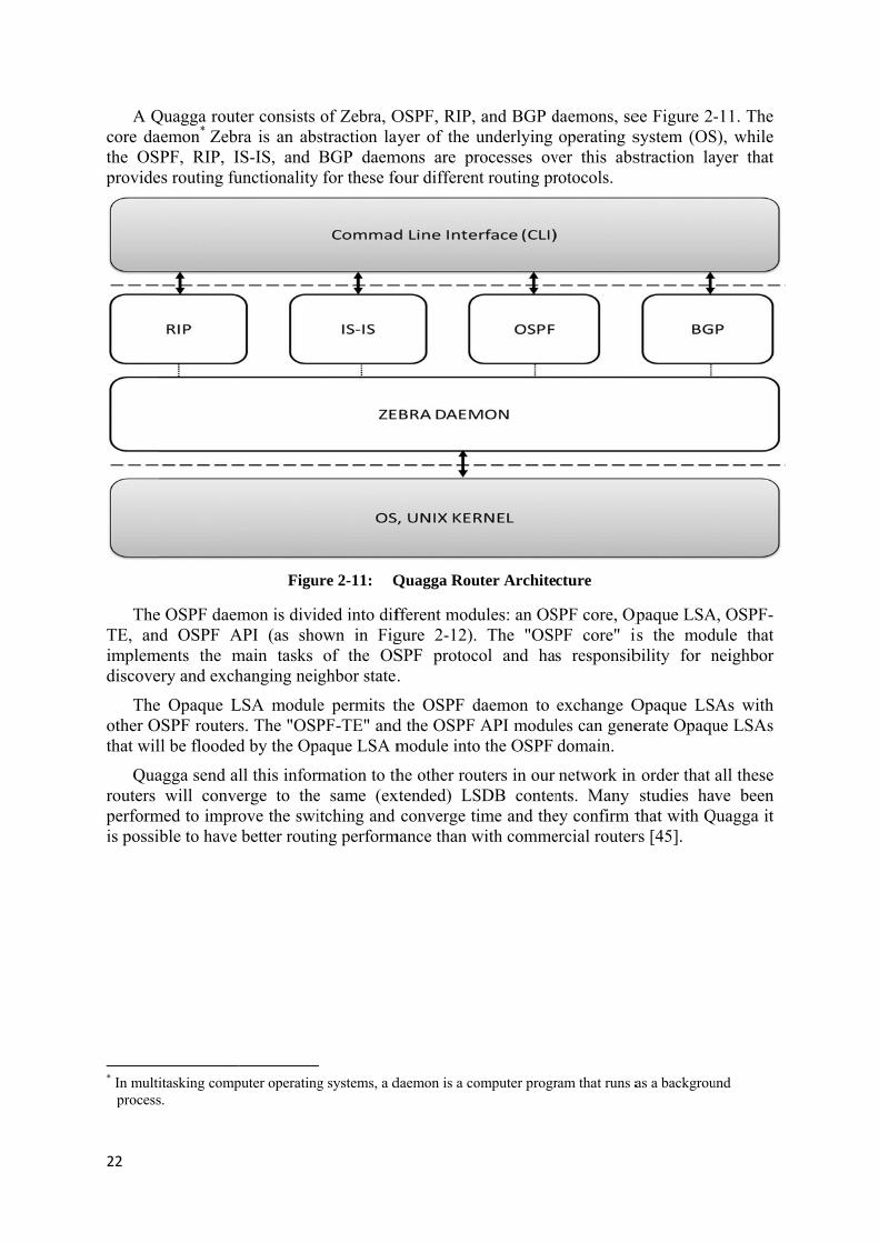
22
A Qcore dathe OSprovide
TheTE, animplemdiscove
Theother Othat wil
Quarouters performis possi
* In multi
process
Quagga routaemon* ZebrPF, RIP, I
es routing fu
e OSPF daemnd OSPF Aments the mery and exch
e Opaque LOSPF routerll be flooded
agga send awill conve
med to imprble to have
itasking comps.
ter consists ra is an absIS-IS, and unctionality
Figu
mon is dividAPI (as shomain tasks hanging nei
LSA modules. The "OSPd by the Op
ll this inforerge to theove the swibetter routi
puter operating
of Zebra, Ostraction layBGP daem
y for these fo
ure 2-11: Q
ded into difown in Fig
of the OSghbor state.
e permits tPF-TE" and
paque LSA m
mation to the same (exitching and ing perform
g systems, a d
OSPF, RIP, yer of the u
mons are prour differen
Quagga Rou
fferent modgure 2-12).SPF protoc.
the OSPF dd the OSPF module into
he other rouxtended) LS
converge timance than w
daemon is a co
and BGP dunderlyingrocesses ovnt routing pr
uter Archite
dules: an OS The "OSP
col and ha
daemon to API modul
o the OSPF
uters in our SDB contenime and the
with comme
omputer progr
daemons, seoperating s
ver this absrotocols.
cture SPF core, OpPF core" is responsib
exchange Oles can genedomain.
network in nts. Many ey confirm tercial router
ram that runs a
ee Figure 2-system (OSstraction la
paque LSAis the modbility for n
Opaque LSerate Opaqu
n order that studies havthat with Qrs [45].
as a backgrou
-11. The S), while ayer that
A, OSPF-dule that neighbor
As with ue LSAs
all these ve been
Quagga it
und

23
Figure 2-12: Quagga OSPF Daemon Architecture
2.6.2 OSPF API Extension The OSPF API is divided into two parts: OSPF API-Server and OSPF API-Client. The
OSPF API-Client can establish a TCP connection with the OSPF API-Server using the OSPF API Protocol [46]. Using this API, applications can get the complete or partial of the LSDB of the OSPF daemon. Additionally, they can originate application-specific LSAs. Opaque LSAs are then transparently distributed to other routers within the LSA’s flooding scope and can be received by other applications through the OSPF API.
External applications connect via the OSPF API client library. The OSPF client library provides an API that directly accesses the LSDB and can transparently distribute customized Opaque LSAs. Given a request from an external application, the client library establishes a connection to the OSPF daemon to retrieve LSA updates and emit Opaque LSAs. The OSPF API server module can handle multiple clients concurrently.
The OSPF API protocol phases are explained below and illustrated in Figure 2-13: Connection initiation The connection between the OSPF API-Client and the OSPF API-Server
is based on two channels: one for synchronous and the other for asynchronous messages. Requests operate synchronously using a two-way scheme, while notifications operate asynchronously by sending messages one-way from either the server or the client. These notifications are one-way messages and can be a result of new, updated, or deleted LSAs received via the network, changes of neighbor connectivity, or failures of interfaces.
Link-state database synchronization
After communication has been established between the OSPF API-Client and the OSPF API-Server, the client application can send a LSDB synchronization request to the server. The OSPF API-Server will send its entire internal LSDB by sending a sequence of LSAs update notifications to the OSPF API-Client.
OSPF API Client OSPF API Server OSPF - TE
Application Opaque modules
OSPF Core LSDB
OSPF Daemon
Zebra Daemon
10.0.0.0/2410.0.0.32/3010.0.0.12/30
eth0eth1eth2
OPSF API Protocol
OSPF Protocol (LSUpd)
Route prefix updates
Interface up/down
Kernel forwarding table updates

24
Opaque type registration Once LSDB synchronization has been achieved, the OSPF API-Client can register the Opaque type which it wants to originate as an Opaque LSA.
Origination of own Opaque LSAs
Once the OSPF daemon has learned that an Opaque-capable neighbor’s state is complete, then the OSPF API-Server will notify the OSPF API-Client that it is ready to flood Opaque LSAs. There must be at least one Opaque-capable neighbor before a router can originate Opaque LSAs. The OSPF API-Client application can originate its own Opaque LSAs and then invokes the OSPF demon to flood them throughout the OSPF network.
Update own Opaque LSAs
The OSPF API-Client can update the content of self-originated LSA and asks the OSPF API-Server to re-flood it with new content.
LSA updates from neighbors
Whenever an LSA of any type is received over the network, the OSPF daemon immediately notifies all applications.
Deletion of own Opaque LSA
The OSPF API-Client application can delete its Opaque LSA from all OSPF routers by sending a deletion request to the OSPF API-Server.
Connection shutdown When an application terminates, it should first delete all self-originated Opaque LSAs before it shuts down its connection to the OSPF daemon. If the application closes the connection without issuing delete requests, then the OSPF daemon takes care of cleaning up obsolete Opaque LSAs, making sure that no stalled Opaque LSAs remain within the network.

Figure 22-13: The
OSPF API Protocol phhases[46]
25

26
2.7 Related work In this section, several previous studies conducted in areas relevant to this master’s thesis
are summarized. This previous research can be divided into the following topics: Congestion Flow Control in a RAN, Congestion Notification in a RAN, I2RS, and Monitoring & Flooding Methods.
In the field of the Congestion Flow Control, Rácz, Pályi, and Nádas researched mechanisms to control and identify congestion in the RAN, but their studies were limited to the performance of transport network layer and the associated data packets flows. Rácz, Pályi, and Nádas [47] describe two different methods that when combined improve the performance and fairness of the congestion identification of the transport flows.
Nádas, Nagy, and Rácz have also worked on congestion identification and avoidance for the air interface, specifically with HSUPA [48], [49]. In this research they propose a per-flow HSUPA transport network flow control algorithm. All of their flow control studies are related to the topic of this master’s thesis, but they do not cover the same breath as our work.
Work has been done to identify and notify entities of congestion in the RAN. Kekki [50] has researched and patented a method, apparatus, and system to notify entities of the occurrence of congestion in a 3G radio access network. This work could be a good combination with the approach proposed in this master’s thesis, because while Kekki focuses more on radio access network congestion notification, this master’s thesis focuses more on the identification of radio access transport network congestion. Companies are also working and researching in transport TE. ARISTA has developed a network analyzer LANZ [51] that provides queue congestion notification in the network with a granularity of microseconds. Ericsson has continued research in this field and one of the last documents is a U.S. Patent application P10259PC00 [16]. The ideas described in this patent application were the starting point for this master’s thesis. By combining the methods and procedures proposed in this master’s thesis it is possible to identify congestion in the RAN and provide this information to the system as this patent application proposes. In combination with the two previous patents and the work presented in this master thesis, we introduce a complete congestion avoidance method and set of control management tools which provide different functionalities, for example improved handover control.
Active control and management of the RAN is becoming more and more relevant as the demands on this network increase. To provide network nodes with the ability to react to congestion and interact with the different control modules of the network is a major research challenge. The AQM tools have helped with this task as Pacifico et al. discuss in [15], but the next step in network management is to provide an I2RS to the network to enable management of the network. As explained in Section 0 the IETF is still developing I2RS and many drafts have been released [34]–[36]. With the functionalities of this new interface and the methods that this master’s thesis proposes to provide congestion information, it should be possible to manage all this information, react, and interact with the network nodes in order to avoid and control the congestion in any module of the RAN.
Another topic related to this master thesis is monitoring and flooding methods. Keller [46], [52] has proposed a client-server method for use in the router node. This solution has been adopted in this master’s thesis project in order to acquire the monitored information and then, forward and flood this information to the rest of the network. This method, as explained previously in the OSPF API Extension Section 2.6.2, was implemented by Keller in the Quagga routing software. This implementation provided us with an important and helpful resource. Amir Roozbeh has also supported and used, in his master’s thesis [53] the work of

27
Keller and, in the same way as this master’s thesis proposes, he has used OSPF-TE TLVs to flood a network with information about monitored resources. While the research field of Amir Roozbeh´s master’s thesis is completely different from the RAN, his work and Amir himself have provided ideas to this master’s thesis project with respect to monitor the congestion of resources and flooding this information into the network.
Finally, a lot of research has been done in order to select the most suitable method to monitor the different resources of the network. This discussion is extended in the next chapters of this master’s thesis. Earlier studies have been made in order to measure the delay [54], [55] and bandwidth [56]. This research has been taken into account as we tried to select our method to monitor these and other properties of the resource of the network.

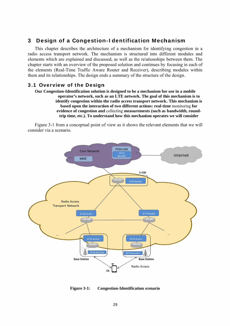
3 DeThis
radio aelementchapter the elemthem an
3.1 OOur
Figuconside
esign os chapter d
access transts which arstarts with
ments (Reand its relatio
Overviewr Congestion
opiden
bevid
tr
ure 3-1 fromer via a scen
f a Condescribes thsport netwoe explainedan overview
al-Time Traonships. The
w of then-Identificaterator’s net
ntify congestbased upon tdence of con
rip time, etc.
m a conceptnario.
Figure
gestione architectu
ork. The md and discusw of the proaffic Awaree design end
e Designtion solutiontwork, such tion within tthe interactingestion and.). To under
tual point o
3-1: Con
29
n-Identure of a me
mechanism issed, as weoposed solue Router ands a summa
n n is designedas an LTE nthe radio acion of two did collecting mrstand how t
f view as it
ngestion-Ide
tificatioechanism fois structurell as the rel
ution and cond Receiverary of the st
d to be a menetwork. Th
ccess transpoifferent actimeasurementhis mechan
t shows the
entification s
on Mechor identifyind into diffelationships bontinues by r), describinructure of th
chanism forhe goal of thort networkons: real-timnts (such as ism operate
relevant ele
scenario
hanism ing congestferent modubetween thfocusing inng modulesthe design.
r use in a mohis mechanisk. This mechme monitorinbandwidth,
es we will co
ements that
tion in a ules and em. The
n each of s within
obile sm is to
hanism is ng for , round-nsider
t we will

30
Two new elements are introduced in the proposed Congestion-Identification solution: the Real-Time Traffic Aware (RTTA) Router and the RTTA Receiver: RTTA Router The RTTA Router is an extended router which has the same functionalities as a
“normal” router in such network, but has an extension for measuring and forwarding relevant information regarding its interfaces. This type of router is located at all the nodes of the radio access transport network, as well as in the S-GW and the base stations.
RTTA Receiver This is a new element is located in the PDN-GW and in the base stations. This element is responsible for detecting evidence of congestion in real-time and collecting the information forwarded by the RTTA Routers. The RTTA Receiver also combines and presents the information in a suitable way in order to enable further actions (e.g. dropping some UEs’ connections or initiating a handover for one or more UEs).
The mechanism presented exploits the interaction of two sub-mechanisms: one based on ECN and the other on OSPF-TE. The information provided by these two sub-mechanisms is integrated by the RTTA Receiver.
On one side, ECN communication occurs between the PDN-GW and the base station in order to detect congestion in real-time as was described in Section 2.2.2. The RTTA Routers mark packets depending of the state of its queues and the selected policy. The RTTA Receivers detect evidence of congestion as packets pass through the PDN-GW or base stations. At the same time, via the other sub-mechanism, each RTTA Router is measuring relevant information (e.g. available bandwidth, one-way delay, round-trip time, number of packets marked, etc.) for each one of its links. This information is flooded over the network using OSPF-TE Opaque packets depending upon the policies implemented in the RTTA Routers. Thus, each RTTA Router maintains updated information about all of the other nodes in its OSPF-TE database and the receiver simply accesses this information via one of the RTTA Routers, usually the closest one. Finally, the RTTA Receiver combines the information from the ECN connection with measurements from each node, in order to characterize congestion in the network. This is presented in two different ways: in real-time and periodically.
The next sections of this chapter describe this mechanism in greater detail by defining each element together with its new modules and its interactions with other modules.
3.2 Real-Time Traffic Aware Router The Real-Time Traffic Aware Router (RTTA Router) is one of the main elements of the
proposed Congestion-Identification solution. This element provides congestion information to the whole network. In order to supply this information, it must be situated in all the routing nodes of the radio access transport network, including the routers situated in the eNodeBs and the S-GWs. The RTTA Router element is divided into the following modules: measuring, monitoring and policies, RTTA sender, and OSPF router. Together these modules measure the congestion of resources associated with each interface of the routing node.
The design of the mechanism proposed has been done using the OSPF-TE protocol, but it is worth mentioning, that other protocols can take its place in a real scenario. The Interior Gateway Routing Protocol (IGRP) [57] and its optimized version Enhanced IGRP (EIGRP) [58] provides similar updating and neighboring detection features as OSPF, and despite they don’t warranty the use of the best route they are easier to configure than OSPF. These protocols also spread the traffic over the network and discover different paths between source and destination, but two main factors provoke its denied: They are Cisco property what

31
implies that its use is more restricted [59] than OSPF and furthermore, the stable implementation of the OSPF-TE in the open source routing software convinced the work team to choose this protocol and the features that it provides as the more suitable one for this design.
By using the OSPF-TE protocol, the RTTA Router constructs a TLV; includes it in an Opaque LSA and injects this LSA into the network in order to flood the radio access transport network with information concerning the congestion observed by this router node. The result is that all routers have an updated database with the relevant congestion information (even performance information) for all of the links of every router in the radio access transport network. Figure 3-2 shows the modules of a RTTA Router. Each of these modules will be explained in detail in the following sections.
Figure 3-2: Architecture of the Real-Time Traffic Aware Router
3.2.1 Measuring The first module has the task of measuring the traffic for all the interfaces of the RTTA
Router. For each interface, it measures selected traffic parameters.
In order to obtain this data the module has to identify the interface. This is done utilizing SNMP. We will use the (first) IP address bound to this interface as the identifier for a set of measurements. This set comprises the available bandwidth, the one-way delay, the RTT of the link that is connected to this interface; and the number of packets marked by the Random Early Detection (RED) queue as Congestion Experienced (CE) packets. The design of these different measurements required more research. Details of this research will be explained in this section and section 4.1.
3.2.1.1 Available Bandwidth Many ways to measure the available bandwidth have been studied. Some tools such as
Pathchar [56] or BART [60] have been considered as possible ways to measure this parameter, but the main problem of these methods is that they load the link by sending a number of probes, thus adding more traffic to what may be an already congested link. Unfortunately, adding more traffic in this situation is counter-productive. These methods were mainly designed to be used to discover the available bandwidth along a whole path (for example, from the eNodeB to the S-GW). These methods are not very convenient for measuring the bandwidth of a link.
Real-Time Traffic Aware Router
Measuring Monitoring &
Policies RTTA Sender OSPF Router
Extended OSPF Router

32
We decided to use the SNMP, as SNMP can directly provide the number of bytes sent and received by each interface. Given this data we can simply calculate the arithmetic mean, from which the total bandwidth used can be obtained. If the total bandwidth of the link is known, then the used bandwidth can be subtracted from this total bandwidth, to give the available bandwidth.
This choice was made in order to provide a simple (simply access a SNMP counter and perform the arithmetic operations) and lightweight (because the network is not loaded with any additional packets) method to obtain the available bandwidth. If the available bandwidth for a whole path is desired, then the tools referred to above are better options – or within the radio access transport network we can exploit the fact all of the routers know the available bandwidth for each link, hence they can simply compute the minimum link bandwidth along any path.
3.2.1.2 Round-Trip Time and One-Way Delay
In order to identify congestion of a link, the measurement of the link delay provides essential information. Two possible ways to learn this delay were considered: measure the one-way delay (the latency from a router to its neighbor) or measure the RTT (the round-trip time of a packet from a router to its neighbor and the return). Both measurements provide sufficient information to identify congestion, but are conceptually quite different. For instance, RTT also provides information about the time required for the forwarding processing in the neighbor router. Using one-way delays measures both uplink and downlink delay separately. These two different latencies can be quite different depending upon the current network conditions. For making one-way delay measurement it is mandatory to synchronize all the nodes’ clocks in the network. Fortunately, we can use NTP at each node of the network to synchronize the local node’s clocks with a single NTP server. Now that all of the clocks are synchronized we can measure the one-way delays to each neighbor.
The measurement method has two different alternatives: one based on communications between routers to share timestamps and the other using TCP timestamps.
In the first method, each router sends another router its current time in a timestamp. Figure 3-3 illustrated the sequence of messages of the proposed design.

Figure 3
For RTT areach coeach roequationwhen ea
AfteThese trouter wcomput
TheTimestaand accrequiresHowevethat the
One
RTT
3-3: Sequone-
each mease measured
ontaining theouter is ablns given inach measure
er the N prtwo averagewaits for a te the next tw
e alternativeamp field tocurate meass sequenceser, if this tim
e timestamp
e-Way Del
T
uence of me-way delay,
surement N d by each ene timestample to compn Table 3-1e is obtaine
T
robes, the es provide t
predefinedwo values.
e method uso the TCP hsurement os of packetmestamp is
p needs to b
lay
essages betwbased on sh
probes arend of the linp of the rou
pute the RT1. In additiod.
Table 3-1:
averages ofthe input vad gap time
ses TCP timheader. Usi
of both routs and its onot already
be inserted i
ween two rouharing route
e sent. Usinnk. Each prouter who senTT and oneon, Table 3
Timestam
f these twoalues for thebefore it p
mestamps, aing this pround-trip andoperation is y in the TCPinto the TC
Client
(
(
uters, R1 anr timestamp
ng each proobe consistsnt this packee-way delay3-1 and Fig
mp Equation
o series ofe next moduperforms an
as describedcedure it is
d one-way similar to
P packet heaCP packet h
(1)
(1)
nd R2, for mps
be the one-s of three paet. Using thy as it is dgure 3-3 in
ns
measuremeule in the R
nother set o
d in section possible todelays. Thithe method
ader, then theader. Unfo
S
measuring R
-way delay ackets of sahese three mdescribed w
ndicate the
ents are coRTTA Routof measurem
n 2.5.1, by ao provide a
his mechanid describedhis method ortunately, t
ender (2) (2)
33
RTT and
and the ame size, messages with the moment
omputed. er. Each ments to
adding a reliable
ism also d above. requires this will

34
increase the processing in the routers, but has the advantage that it can be piggybacked on top of existing traffic – hence only requiring the number of bytes for each timestamp to be added to existing packets. This approach discussed in detail in section 4.2.1, but due to software limitations of the nodes used in the test-bed, the first alternative was chosen for this the measurements used in this thesis.
Other active methods could have been chosen, as Pathchar or other ICMP based tools [61]. These tools have been researched and considered, but they are not suitable for our solution since they use are designed estimating the bandwidth of paths through network, rather than for individual links. Additionally, according to Strowes [54] these techniques are less accurate than the results provided using a passive method, as a TCP timestamp.
3.2.1.3 Marked packets
The main purpose for measuring this parameter is to identify which nodes have been involved in marking packets after receiving a packet with the ECN congestion experienced bit set. This parameter helps us to identify the congested link. At the beginning of this thesis project, this parameter was not going to be sent. Instead the first choice was to simply send the size of the interface queue. We thought that this parameter could easily be obtained from the MIBs via SNMP, but this method had to be rejected because of limitations of the software used in the test-bed. This alternative will be explained in detail in section 4.2.1as this method could be implemented when using other systems. Moreover, consideration of this method guided us to a similar and complementary solution.
A Random Early Detection (RED) output queue with ECN marking was implemented on each interface. With this design the total number of packets marked as Congestion Experienced can be obtained giving us direct evidence of congestion. This method is more intuitive than the queue size parameter that was studied early in this thesis project.
As it has already said, the set of measurements is made for each interface. When the module has finished measurements for each interface it passes this information on to the next module.
3.2.2 Monitoring & Policies The next module implemented in the RTTA router has two tasks: monitoring and
deploying policies. Throughout this explanation this module is also referred to as the monitoring or decision module, depending on which task is being considered at that moment, although both functionalities are found in a single module. After the measuring module, the router continues monitoring in real-time the measurements that have been made. This monitoring module, for each router interface, receives the latest set of measurements and then decides if the information is relevant to send to others. If the changes in measurement values are determined to be relevant, then the router will forward these measurements to the next module, otherwise the latest measurements will not be forward.
The importance of this decision module is worth mentioning as it prevents the unnecessary flowing of updates that might unnecessarily load the network. To avoid this, the decision module implements policies to determine for each of the different parameters measured when a change in the measurements is relevant to other nodes in the network. The implementation of these policies is explained in the next chapter. Here we simply state that if any of the measurements has a relevant change, then the whole set of measurements are forwarded regardless of whether they have changed or not.

35
3.2.3 Extended OSPF Router This module is divided in two sub-modules: RTTA Sender and OSPF Router. The RTTA
Sender constructs the Opaque packet while the OSPF Router floods the LSA to the network.
3.2.3.1 RTTA Sender
The RTTA Sender sub-module is one of the two sub-modules of the module that extends the standard OSPF router module. The main task of this sub-module is to build an Opaque LSA packet with the relevant traffic congestion information obtained from the previous modules. Section 2.3.4 gives the necessary background about the construction of this packet. The LSA type field is 10 because the Opaque LSA is to be flooded throughout the whole OSPF area. The Opaque Type chosen is type 1, as this corresponds to a Traffic Engineering LSA and this packet contains information relevant to traffic control. The next field is a TLV. The TLV type is 5 because the packet contains Node Attributes, and finally a sub-TLV with type 4, an unassigned sub-TLV type [32]. In this final field the set of measurements are included, as shown in Figure 3-4.
LS Age Options 10 1 Opaque ID
Advertising Router LS Sequence Number
LS Checksum Length Type 5 Length Type 4 Length
Interface IP RTT
One Way Delay Available Bandwidth
Number of ECN Marked Packets Figure 3-4: LSA-Opaque Packet
The details of the construction of this packet were a major point of discussion and research by the team. Many options were researched, three of which are shown in Figure 3-5. Instead of sending only one sub-TLV with the parameters as shown in Figure 3-5 (a), two other options could have been chosen: send the parameters in a different sub-TLV field each one but in the same packet Figure 3-5 (b) or simply send one parameter in each sub-TLV and packet Figure 3-5 (c). Each of these alternatives has its own benefits and weaknesses. Selecting the best alternative requires additional research and analysis which are out of scope of this thesis project. In this master’s thesis project we have followed the advice and research of Amir Roozbeh [53] and placed the parameters in the same TLV field and in the same packet. This alternative us allows to distinguish the measurements of each interface based upon the IP address of interface, thus, a larger sub-TLV is a better solution that the other alternatives.
TE Header
Node Attributes
TLV Sub-TLV

36
It ispreviouthe polithose phas a rethe effo
WhOSPF R
(a)
(b)
(c)
s worth menus module. Iicy would carameters, elevant chanort to send o
en the OpaqRouter.
Figure 3-
ntioning thaIf we had chcheck if eacinstead of fnge, was do
one paramet
que LSA is
5: Three
at this decihosen to sench parameteforwarding one in this dter is nearly
created it i
e alternative
sion has a nd just one per has had a
all the pardesign. Thi
y the same e
is forwarded
...
e Sub-TLVs
big influenparameter ia relevant cameters whis decision wffort as requ
d to the nex
proposals
ce on the dn one TLV hange and w
hen any onewas supporuired to sen
xt sub-modu
decision tasin one packwould forwe of the parrted by the nd all of them
ule of the E
k of the ket, then
ward just rameters fact that m.
Extended

37
3.2.3.2 OSPF Router
The last sub-module of the Extended OSPF Router is also the last step performed by the RTTA Router. This module plays the role of a “normal” OSPF router. When it receives the LSA built in the previous sub-module, it will inject this LSA into the OSPF network in order to flood the area with this traffic information.
As an OSPF router, it has all the functions and features of an OSPF router. One of these functions is to create a forwarding table with the information necessary to route packets that arrive at this router. To do this it creates a database containing all of the sub-nets of the network, its neighbors, and the shortest path to reach each sub-net. Another feature, essential to understand the design of the elements of this network, is that an OSPF router has the functions necessary to create a TED. This TED contains information from all the Opaque LSAs with TE information that was flooded to the network. Thus, a RTTA Router that injects Opaque LSA packets in the network is at the same time receiving Opaque LSAs from the other RTTA Routers and updating its TED based upon the information that these packets contains.
3.2.4 RTTA Router Summary After the above explanation of the RTTA Router, it is worth summarizing the main ideas
and the features that this router realizes. This RTTA router collects relevant traffic information (bandwidth, latency, and ECN marked packets) from all of its interfaces and floods the network with this information, thus all the traffic information from all the interfaces of all the routers in the network is stored a TED at all of the routers in the network. Therefore, except for periods of convergence the same information should be stored in all of these TEDs.
3.3 Real-Time Traffic Aware Receiver This section describes the design of the RTTA Receiver and its role in the proposed
Congestion-Identification solution. The RTTA Receiver may be located in both PDN-GWs and the eNodeBs. In this way, the information collected by the RTTA Receiver can help these nodes to manage and handle the traffic associated with UEs making use of the PDN-GW and eNodeBs. This element is responsible for integrating the two sub-mechanisms described above (i.e., OSPF-TE information and the CE detection), by collecting, sorting, and analyzing the information that has been obtained.
The RTTA Receiver can be divided in two modules (as shown in Figure 3-6): one for collecting all the congestion information and another in which the integration and analysis are performed. Figure 3-6 illustrates the architecture of the RTTA Receiver and the relationship between the two sub-modules. In the “Collecting of Congestion Information” module, the RTTA Receiver accesses the TED of the router situated in the same node as it (i.e., eNodeB) or to the closest one in case of none router is not located in either of both entities; and at the same time, it acts as a detection module (as described in the case of an ECN connection in section 2.2.2). Then, this information is processed by the RTTA Receiver in the “Analysis and Visualization” module, in which information is sorted and analyzed from two different perspectives: in real-time (where the information is processed as it is collected) and periodically (i.e. information is captured for a period of time and stored for subsequent analysis).

38
3.3.1
As detectiomoduleOSPF-T
CE detec
Thedifferen
3.3.2
Thisinformaand the The pur
* Howeve
determi
Figur
Collectinstated earl
on. Both ofe. TE Receiver
ction module
e collected int actions or
Analysis s is the moation occurs evidence orpose of th
er, since the uined to be rele
e 3-6: Ar
g of inforlier, this mf them gath
The Oinformamaintaimeasurdynamibetweenfrom thOpaqueReceivethe LSARoutersfloodinto hand
e The CEpacketsthe recpairs ofin betwpolicies
informationr decision m
and Visuodule of ths. The inforof congestiohis module
update containevant there ma
rchitecture o
rmation mmodule has her congesti
OSPF-TE Ration locatedins an updatrements forically accesn the OSPF-he moment e LSA from er downloadAs on the flys for decidin
ng the networdle redundantE detection ms marked (byeiver is locaf PDN-GW
ween them mas selected in
n is deliveremaking.
ualizationhe RTTA Rrmation fromon detected is to help t
ning all of the ay be some am
of the Real-
module two funct
tion informa
Receiver fud in the TEDted TED, du
each link ss and dow-TE Receivethat the RTany of the ot
ds it. This desy, is consisteng when a nrk with unnet informationmodule is iny sniffing CEated. It is woand eNodeBark packets dthose nodes
ed to the ne
moduleReceiver, thm the measueither in ththe eNodeB
parameters is mount of hand
-Time Traffi
tionalities: ation that w
unctionality D of a RTTue to the use
of the netwnloads this er and the RTTA Receivther routers asign, in whic
ent with the inew Opaqueecessary Opan*. n charge of dE packets) inorth to ment
B an ECN codepending o.
ext module
he last step urements cae PDN-GW
Bs or PDN-
sent if any ofdling of redund
ic Aware Re
OSPF-TE will be the
is responsTA Router. Ee of OSPF-Twork. The
database. TTA Routerer starts to arrives in the
ch the RTTAnclusion of pe LSA shouaque LSAs an
detecting CEn the interfactioning here onnection is sf the state of
for analysis
in processarried out in
W or the eNoGW take fu
f the parametedant informati
eceiver
Receiver input for t
sible for cEvery RTTATE mechaniOSPF-TE
The commur remains eswork. Whe
e TED, the OA Receiver do
policies in thuld be sent, and reducing
E packets by ce of the rout
that betweesetup and thf their queue
s, visualiza
sing the conn the RTTAodeBs is profurther actio
er changes aretion.
and CE the next
collecting A Router sm, with Receiver unication tablished n a new
OSPF-TE ownloads he RTTA avoiding the need
tracking ter where n logical
he routers s and the
tion and
ngestion A routers ocessed. ons. The

39
analysis and visualization module has been separated into two sub-modules: one for real-time processing and the other for periodic processing. The reason is to exploit the latest update about network properties in real-time actions; while in parallel being able to study the behavior of the network for periods of time in order to consider other types of actions that concern longer term properties or to guarantee stability for a longer period of time.
• The real-time functionality monitors the state of the network by comparing the parameters (available bandwidth, RTT, one-way delay, number of packets marked) for each link of the network and computing from them different characterizations of the state of the network. At the same time, an ECN indication monitors the number of marked packets detected by the RTTA Receiver to complement the information about how many packets were marked by each of the routers.
Many characterizations can be considered here, such as comparing the information by interface, router, link, or path. However, the current design of this module focus on presenting the information aggregated by paths, since this is a convenient characterization of the congestion information in a network, as will be discussed in later chapter. This visualization gives agile feedback about the traffic conditions of the radio access transport network that potentially allows elements of the mobile network (such as eNodes, PDN-GW, or MME) to make optimized decisions, such as initiating a handover or dropping one or more packets in order to guarantee end users a high QoE.
• Periodic Analysis consists of study the network properties over a period of time. Many characterizations can also be considered here. Following the same modus operandi as in real-time analysis, we focus on comparing the congestion information of different paths through the network. In this way, we hope to observe trends of the measured parameters in order to understand the behavior of the network over a longer period of time. The purpose of this functionality, besides monitor the traffic conditions over a period of time, is to study if actions motivated by the real-time analysis module are consistent with keeping the network stable over a longer period of time.
3.4 Summary of the design Throughout this section, the design of the proposed Congestion-Identification solution
has been described, giving the reader the necessary background to understand how this proposed solution works. Subsequent chapters will describe how this solution has been realized in a prototype and analyzed by using a test bed.
The proposed solution is based on the coexistence of two sub-mechanisms and their interactions. The RTTA Routers measure, monitor, decide upon relevance, and inject Opaque LSAs with information about RTT, one-way delay, bandwidth, and the number of ECN marked packet at each interface to its links. By this method, the relevant congestion information of the whole routing system is located in all the nodes of the network. In order to access to this information, this design performs a unique communication between the router and the receiver that allows transferring state out of the routing system, following the I2RS mechanism described in the background section 2.4.
With this interface designed between the RTTA Receiver (I2RS Client) and RTTA Router (I2RS Agent), the RTTA Receiver is able to access to the information of the whole routing system, due to this information obtained from all of the other nodes that is stored in the TED of each RTTA router of the network.

40
Additionally, ECN connections are enabled in the network which the RTTA routers mark in case of congestion and the RTTA Receiver evaluates this evidence. Finally, the RTTA Receiver integrates all this information by analyzing it and presenting it both in real-time and periodically.
In summary the proposed solution creates an updated map of the state of the network including information about the congestion state of each of its links. Subsequent chapter give some examples of show how this information can be utilized.
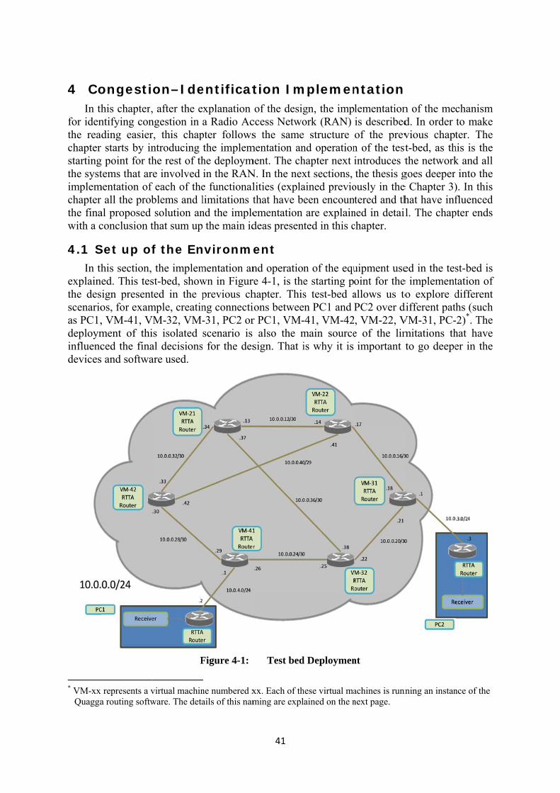
4 CoIn th
for identhe reachapter startingthe systimplemchapter the finawith a c
4.1 SIn th
explainthe desscenarioas PC1,deployminfluencdevices
* VM-xx
Quagga
ongestihis chapter,ntifying conding easierstarts by in
g point for thtems that ar
mentation of all the prob
al proposed conclusion t
Set up ofhis section, ed. This tes
sign presentos, for exam, VM-41, Vment of thiced the finas and softwa
represents a v
a routing softw
on–Ide, after the engestion in r, this chapntroducing he rest of thre involved f each of theblems and lsolution an
that sum up
f the En the implemst-bed, showted in the p
mple, creatinVM-32, VM-is isolated al decisionsare used.
F
virtual machinware. The deta
entificatxplanation a Radio Ac
pter followsthe implemhe deploymin the RANe functionallimitations tnd the imple the main id
nvironmmentation anwn in Figurprevious chng connecti-31, PC2 orscenario is
s for the des
Figure 4-1:
ne numbered xails of this nam
41
tion Imof the desig
ccess Netwos the same
mentation anment. The chN. In the nexlities (explathat have beementation deas presen
ent nd operationre 4-1, is thehapter. Thisions betweer PC1, VM-
also the msign. That i
Test bed
xx. Each of thming are expl
mplemengn, the impork (RAN)e structure nd operationhapter next xt sections, ained previoeen encounare explainted in this c
n of the eque starting ps test-bed a
en PC1 and -41, VM-42main sourceis why it is
d Deploymen
hese virtual maained on the n
ntation lementationis describedof the prevn of the testintroduces tthe thesis g
ously in thetered and th
ned in detailchapter.
uipment useoint for theallows us toPC2 over d, VM-22, Ve of the limimportant t
nt
achines is runnnext page.
n of the med. In order vious chaptt-bed, as ththe network
goes deepere Chapter 3)hat have infl. The chap
ed in the tese implemento explore d
different patVM-31, PC-mitations thto go deepe
nning an instan
chanism to make ter. The
his is the k and all into the
). In this fluenced
pter ends
st-bed is tation of different hs (such
-2)*. The hat have er in the
nce of the

42
The realization of this scenario is done using five physical machines (see Table 4-1). Three of them host two virtual machines inside each of them. Each of these virtual machines plays the role of a router. The result is that we have emulated a total number of 6 routers in this test-bed. Two other machines play the role of end-nodes (in this scenario they emulate an eNodeB and PDN-GW) forming in this way a complete Radio Access Transport Network. The OS used in all the machines is Ubuntu 12.04 with Kernel 3.5.0-41-generic [62] and the virtualization software used to realize the virtual machines is Virtualbox-4.3 [63].
The routers are named with a number consisting of two digits, where the first digit indicates the host and the second digit indicates the number of the virtual machine (guest) inside that host. The end-nodes are called PC1 and PC2 playing the roles of the eNodeB and the PDN-GW (respectively). All the machines are physically interconnected using Cat 5-E [64] Ethernet cables connected to Ethernet interfaces configured to operates at 1000 Mbps, thus the maximum available bandwidth of each of these links is 1000Mbps.
Although the interfaces of the hosts are connected by these physical links, the guests inside them are linked by UDP tunnels. This is networking mode provided by VirtualBox to interconnect virtual machines running on different hosts[65]. This is done by encapsulating the Ethernet frames (sent or received) by the guest network card into UDO/IP datagrams, and sending them over the interface assigned to this guest interface. In order to configure this tunnel, the network adapters of the guest must be configured as generic drivers with UDP tunneling and the host’s IPs interfaces must be the same to the corresponding one of its guest. Furthermore, it must be also configured the source and destination UDP port and the destination address, being this parameters swapped with the corresponding virtual machine in the other host. Thus there is one (virtual) network adapter for each of the guest’s network interfaces. With this mode, each guest network adapter acts as if it is directly connected through a physical network interface to its (virtual machine) neighbor.
To interconnect the two guest VMs running on the same host, Virtualbox provides a different type of connection. An internal connection is created to pass the information from one guest to the other. VirtualBox also allows limiting the bandwidth of these internal links[65], providing a good mechanism to provoke different scenarios and simulated bottlenecks.
Once all the nodes are interconnected, each router has to build its forwarding database to route the traffic in this network. To provide this functionality to the elements of our network the routing software Quagga is installed in all virtual machine. With this software, as explained in the 2.6 section, an IP address is associated with each interface of the network via the Zebra daemon. With Quagga running in all the routers of the area, we can divide the area into different sub-networks and run the OSPF protocol over the network. The main reason to implement OSPF (explained in the 2.3 section), rather than another routing protocol in this scenario, is the traffic engineering features that OSPF provides. By running OSPF-TE in the area, the shortest paths will converge and the forwarding tables are built. Quagga provides also an API to interact with the OSPF router. This API serves as a bridge to inject the generated Opaque TE packets and to access the router’s link state database.
The final step in the initial implementation is to enable ECN in the network. The end-nodes must be able to negotiate the use of ECN. In order to simulate this ECN feature in a Radio Access Transport Network, as it has been explained in section 0, TCP handshaking has been deployed to emulate it. On the other hand, the router nodes must be capable of marking ECN when they are congested. This last issue can solved enabling the router specifically to mark the packets, being this feature provided by the Ubuntu OS, setting the tcp_ecn [66]parameter correctly.

43
Following the above step, the test-bed is up and running. This means that all the initial elements of the network are connected and they can communicate to each other. In the following sections the implementation of the new elements introduced in the design chapter are explained. The RTTA Router is implemented in all of the virtual machines of the test-bed and in both end-nodes. The RTTA Receiver is only implemented in the end-nodes, i.e., the eNodeB and the Gateway. Table 4-1: Configuration of each of the computers used to realize the test-bed
Computer Role Description PC1 eNodeB HP™ EliteBook™ 8560p Intel® Core™ i7-2620M CPU @ 2.70 GHz x
4, with 3.9 GiB memory, Integrated Intel 82579LM Gigabit Network Connection; 500 GB 5400 rpm SMART SATA II HDD[67]
PC2 PDN-GW HP™ EliteBook™ 8560p Intel® Core™ i7-2620M CPU @ 2.70 GHz x 4, with 3.9 GiB memory, Integrated Intel 82579LM Gigabit Network Connection; 500 GB 5400 rpm SMART SATA II HDD[67]
RouterHost2 Hosts VM21&VM22
Dell™ OptiPlex™ 7010 Intel® Core™ i7-3770 CPU@ 3.40 GHz x 8, with 7.8 GiB memory, Integrated Intel® 82579LM Ethernet LAN 10/100/1000; 3.5” Hard Drives: 1TB 7200 RPM SATA[68]
RouterHost3 Hosts VM31&VM32
Dell™ OptiPlex™ 7010 Intel® Core™ i7-3770 CPU@ 3.40 GHz x 8, with 7.8 GiB memory, Integrated Intel® 82579LM Ethernet LAN 10/100/1000; 3.5” Hard Drives: 1TB 7200 RPM SATA[68]
RouterHost4 Hosts VM41&VM42
Dell™ OptiPlex™ 7010 Intel® Core™ i7-3770 CPU@ 3.40 GHz x 8, with 7.8 GiB memory, Integrated Intel® 82579LM Ethernet LAN 10/100/1000; 3.5” Hard Drives: 1TB 7200 RPM SATA[68]
4.2 Real-Time Traffic Aware Router Following the general scheme of this chapter, this section explains the implementation of
the RTTA Router element already introduced in the design chapter. All the modules and their design are revisited in order to go deeper into them. All of these modules, included the modules that Quagga provides, are implemented in the C programming language [69], except for the measurements of bandwidth and the number of marked packets as these two modules are written using Bash scripts [70].
The modules of the RTTA router are situated in different modules inside the Quagga software. As was shown in Figure 2-12: Quagga OSPF Daemon Architecture, when using the OSPF routing protocol the software creates a relationship between a server (included in the OSPF router) and a client. The client is part of an application that can introduce (or receive) information through Opaque TE packets. The implementation of the measuring, monitoring, and policies and the RTTA sender modules have been realized in the RTTA Router application. The OSPF router is actually just the routing part of the Quagga system with server functionality. These separate modules allow us to isolate the traffic engineering mechanism from the actual OSPF routing forwarding making the implementation modular, hence they are easier and safer to handle [52]. Figure 4-2 shows a flowchart which indicates the relationships between the different modules of the RTTA Router.
The three modules (measuring, monitoring, and policies) will each be explained in one of the following subsections. The implementation of the RTTA Sender will be described in section 4.3. The explanation of the deploying of the OSPF Router is unnecessary because it is already implemented in the Quagga system with the API Server functionality. This chapter ends, in section 4.4, with a summary of the implementation of the whole router system.

44
Figure 4-2: RTTA Router Flowchart
4.2.1 Measuring module The first module has the task of measuring three traffic parameters for all of the interfaces
of the RTTA Router. The idea of placing the implementation of these measurements in this module is to make them independent and isolate them from the rest of the modules. This implies that each measure is designed as a sub-module of the measuring module, as shown in Figure 4-2. This independency makes the module more robust and safer, avoiding overwriting and synchronization problems that could occur when implementing the measurements of the three parameters in one module. Additionally, separating the measurements into different sub-modules and handling them separately for each interface, makes the access easier and safer. These advantages lead to this method of realizing these measurements being the most suitable for this project. This approach should also facilitate future additions of additional measurements (if there is a need for them).
At the beginning of each set of measurements; this module has to identify which interface is actually being measuring, this is done by using the IP address of the interface being measured as the identifier. Thus the IP address of the interface is used as (1) the identifier of the set of measurements, (2) it is used by the RTTA Receiver to distinguish the interfaces of the network, and (3) it is used to identify the interface during visualization. This implementation has used SNMP to get the list of IP addresses for the active network interfaces. This approach decouples the implementation from worrying about the name of the interfaces and what their IP address(es) is(are). Given these identifiers the measurements are done as described in the following paragraphs.
Measuring
AvailableBandwidth
Latency
Marked Packets
Monitoring MonitorDatabase
Database Read
IntervalPolicies
RTTA Sender
OSPF API Client
OSPF API Server
OSPF Router
TEDatabase
No
Yes
Packet sent to the network
Packet received from the network
Worth to be sent?
RTTA Router Application

45
4.2.1.1 Available Bandwidth
As explained in the design section, the use of active measurement methods to determine available bandwidth was rejected in order to provide a simple and light mechanism. The alternative method that has been selected exploits the information that SNMP can provide. Because SNMP keeps a number of different counters, we can easily learn the number of packets and bits received and sent by each interface. With this information we can simply calculate an arithmetic average of the total used bandwidth for the interface being measured. This data is collected using called ifstat [71], a tool that the Ubuntu OS provides. Given the configured maximum data rate of the interface and the average total bandwidth used we can simply subtract the used bandwidth from the maximum possible bandwidth 1000Mbps to calculate the available bandwidth.
At the same time, the interface on the other side of the link is also measuring the bandwidth. This implies that at least two measurements of the bandwidth for each link are available. Although these measurements are not precisely simultaneous, if they occur close enough in time we will have an up to date and consistent measurement of available bandwidth. This corroborated information is used in the RTTA Receiver to obtain a more accurate estimate of the link’s available bandwidth. The module will report the bandwidth in units of kbps.
This straight-forward implementation demonstrates the simplicity and lightness of this mechanism. No probe or other packets need to be sent and the complexity of the mechanism is low compared with the other tools and active measurement methods referred to in the design.
4.2.1.2 Round-Trip Time and One-Way Delay
Obtaining the link’s latency parameters via two similar but different methods was explained in section 3.2.1.2. Below the choice of method for the implementation is explained along with the limitations that influenced this decision.
The first method referred in the design chapter, is to make a delay measurement using the TCP Timestamp field included in the TCP header. As was explained in section 2.5.1, the value of this field is exchanged between the two machines at the endpoints of the TCP connection. The granularity of this parameter depends on the endpoint machine’s clock. This implies that the minimum time granularity for a delay measurement using this method is limited by frequency of the clock that the OS uses. More specifically, for the Ubuntu OS used in this test-bed the granularity of the clock is 10 milliseconds [72], because the clock is defined to have a frequency of 100 ticks per second. This accuracy is insufficient for the purposes of this master thesis as a granularity of at least microseconds is necessary to provide a measurement of latency that reflects the link’s congestion.
This limitation has been a factor in rejecting this first mechanism, but it is worth mentioning that in a real scenario this problem can be solved. Other commercial OSs provide clocks with finer granularity, such as Cisco’s IOS [72]. Additionally, the Ubuntu kernel can be modified and recompiled to provide a higher frequency clock, although this option has been discarded to avoid introducing other unexpected TCP issues in our test-bed.
The rejection of the first mechanism leads to our use of the second mechanism to provide link latency measurements. This method can take advantage of the exchange of messages using almost any transport protocol. However, in this thesis only UDP and TCP have been considered due to our familiarity with these protocols. Both of them offer different benefits. UDP allows a light-weight exchange of messages, due to it connection-less behavior; while TCP utilizes reliable connection oriented communication. In this implementation, TCP has
46
been chosen to ensure that the measurements are made, even in case of congestion. Note that in the face of high packet loss rates it is not clear that the measurements will actually be accurate – but they will still have some meaning.
This TCP connection carries client/server communication between the endpoints of a link. The OS clock is read and placed as a timestamp that is send to the other party. This communication is configured to send a specified number of probes via each TCP connection with a specified time gap between each probe.
Since the granularity of the internal clock of the OS is in nanoseconds, then if the synchronization between the machines exchanging messages with such timestamp is tight it is possible to use this method to determine one-way delays. As described in section 3.2.1.2, this synchronization is done using NTP. An NTP daemon was configured in all the machines and all the nodes are synchronized with one of the machines acting as a NTP server. This allows the internal clocks of all of the nodes to converge. Even with this protocol, it was not possible to synchronize the clocks with a granularity of nanoseconds, obtaining Time Errors between nodes (function that calculates the difference in time values of two clocks at a certain time) of more than 1 millisecond. Hence the measurements provided for the One Way Delay do not offer any sensible values, due to the necessity of a precision of microseconds for measuring One-Way Delay in this network. Although, in other implementations using synchronization methods such as Precise Time Protocol (PTP) described in IEEE 1588 [73], which requires specific hardware and software, it is possible to obtain precise network synchronization to an accuracy for at least sub-microseconds, as it is discussed in the Mozhdeh Kamel’s master’s thesis [74]. This issue has led us to ignore the measurements of this parameter, thus only the RTT value is utilized.
Fortunately, the measurement of the RTT does not require synchronization of the nodes. This measurement uses the internal clock of a single node. While RTT values permit us to have a good characterization that there is congestion on the link it does not tell us which direction of the link is experiencing congestion. Additionally, the RTT value measured in the TCP connection implemented here is affected by the processing time in the nodes of the packets.
4.2.1.3 Marked packets
The implementation of the measurement of this parameter requires previous configuration of the queues of the interfaces in the router. These queues must include an AQM mechanism, more specifically a RED one. With RED the queue starts to drop packets with a certain probability, but if ECN is enabled for this queue, then instead of dropping packets it marks the packets with this probability. As a result each output queue is configured with three thresholds and one probability. The thresholds are: the minimum (when the queue starts to mark with the probability indicated), the maximum (when the packets are one hundred per cent marked), and the total limit of the queue. If this total limit is reached, then the packets that arrive to this queue are dropped. The system must also be configured to make it ECN-aware and to enable it to mark the packets while acting as a router or as an end-node for the communication.
As was explained in the design, one first mechanism, that procures the output queue length of each interface, was attempted in order to provide evidence that a queue in the network is marking packets. This value is included as a counter in a SNMP MIB with the name ifOutQLength [75]. With access to this counter we could spread this information to the network, as it provides a direct relationship between the number of Congestion Experienced (CE) packets sniffed in the end-nodes and this queue length parameter.

47
Unfortunately, the use of this SNMP counter is deprecated [75]. Although commercial routers from companies such as Cisco [76] implement this value, in other OSs this counter is not used, specifically the Ubuntu OS used in this thesis project does not implement this counter. In the Quagga routing software this counter is not included nor is it present in the SNMP upgrades [77]. As a result we could not use this parameter, but it is worth mentioning that this limitation is due to the OS used. In a network with routers that implement this counter, this method could be used to provide relevant additional information about the state of the queues.
Due to this setback, another tool, tc (traffic control)[78], was used as it allows us to explicitly manage the queues in Ubuntu. With this tool, not only is it possible to configure the queues of the interfaces as mentioned above, but the tool also provides statics about the traffic going through these queues, including the number of dropped and marked packets. With access to the actual number of packets marked by each interface, the information provided to interact with the sniffing mechanism of the RTTA Receiver is even more descriptive than would have been provided by the queue length parameter!
When the module has finished with the measurements of one interface, it stores the data in separate text files, ready to be read by the next module. These files keep the last measurement of each parameter for each interface being overwritten when a new specific measurement of that interface is done. As we have labeled the measurements with the IP address of the interface and the measurement results are stored independently for each measurement and interface, this module can continues with its task of making measurements of all the interfaces without any danger of overwrite the previously collect information about another interface.
4.2.2 Monitoring & Policies modules This module was been divided in section 3.2.2 based upon the two tasks that it performs.
Consistent with this design we implemented the two tasks as two separate processes that execute concurrently.
The first task monitors the text files with the measurements and writes them in a Sqlite3 [79] database. This sequential mechanism, even if it is not very efficient, allows assuring a problematic-less access and writing in the database fulfilling the requirements of the monitoring. When the information of an interface is read, the monitor fills a row which its columns are the four measures done: the interface IP, the available bandwidth, the RTT and number of packets marked. It does the same for the others interfaces, resulting in a database with a number of rows equal to the number of interfaces, as shown in the Table 4-2. Through this method, the set of measurement overwrites the previous corresponding to that interface, while at the same, the history of all the measurements done, are stored in a trace file. With all the information kept in a unique database, for the next process that it has to be done in this module, only one access to this table is required. This database usage allows to have the measurement data safely stored and at the same time does not need extra time access. This method also let to keep the data from as much interfaces as the node has, just adding more rows to the built database. The mechanism proposed fulfills the necessary requirements for the secure functioning of the module. The study of its efficiency is of the scope of this thesis and future works can be researched in order to improve it.

48
Table 4-2: Sqlite Database Contents
After the information has been stored, the module can make a decision of where the information is relevant enough to be forwarded. This decision is made each time that this database is read. A “Database Read Interval” parameter can be configured to set this cycle. Each read cycle checks all the interfaces. To decide if the information is relevant enough to propagate, the new entry (Rn) is compared with the last relevant reading (Rp). This comparison is shown in equation (1).
= ℎ ℎ (1)
This method is called a relative threshold-based policy [80] and as implemented in this thesis a percentage threshold is selected. This parameter can be separately selected for each type of measurement.
When the database is read the RTT and the bandwidth are checked in keeping with this relative threshold-based policy. If one of the measured values is considered to have a relevant, then the whole set of parameters for that interface are stored as the last relevant measure, and then these parameters are forwarded to the next module.
The number of packets marked does not use this policy because this number only increases and can reach large values for that the threshold chosen, making a relative threshold no longer suitable. In order to provide a constant flow of information, a periodic update policy is implemented when no relevant change has happened. A parameter can be configured as the number of “Database Read Intervals” after which a new update is made even if no single set of measurement has fulfilled the relative-threshold. In this implementation, the previous work of Amir Roozbeh [53] was used to provide a suitable solution for this problem.
4.2.3 Extended OSPF Router module This module is divided into two sub-modules: RTTA Sender and OSPF Router. The
implementation of the second sub-module is not part of our thesis project because is already is implemented in Quagga, hence this section primarily focuses on an explanation of the relationship of these sub-modules through the OSPF API and use of this API to exchange information with other nodes.
4.2.3.1 RTTA Sender
The RTTA Sender sub-module as explained section 3.2.3.1 is one of the two parts of the Extended OSPF Router module. This extension of the OSPF router has the task of building Opaque TE LSAs. The construction of these packets starts from the sub-TLV and continues with the addition of the required headers until the LSA is sent.
When a set of parameters have been accepted by the previous module, the process of constructing an Opaque TE LSA begins. A sub-TLV with type 4 is created to carry this set of measurements as a field of 32 bits each. For a total of size of 5 x 32 bits (4 fields of 32 bits
IP
RTT(ns)
Available Bandwidth(kbps)
Marked Packets
Eth0 10.0.0.25 988623 925424.34 0
Eth1 10.0.0.38 889078 934242.23 30
Eth2 10.0.0.22 1002344 984542.27 70

49
for the IP address and the measurements and then another 32 bits for the Type and Length of the sub-TLV) for this sub-TLV. In the next step a type 5 TLV is added and then the OSPF Opaque header is added with a LSA type 10 (Area Opaque) and the Opaque type 1 (TE).
The Opaque ID field is filled-in during this process. A different value of the Opaque ID is used for each interface in order to provide an identifier that will make it possible in the TE database to distinguish between the Opaque TE LSAs of the different interfaces that come from the same router. Without this identifier the incoming Opaque TE LSAs would overwrite the previous LSAs of a given router even if they are for a different interface.
4.2.3.2 Quagga OSPF API
The Quagga routing software provides a means to communicate between the RTTA Router application and the routing system. As was introduced in section 2.6.2, by using this protocol the application can connect to the router and send the Opaque TE LSAs that it has built, just as if it was the router itself that created the LSA.
Using TCP the client/server endpoints establish a communication session. First the client opens a connection for synchronous request/replies to the server, and then, the server accepts this incoming connection and opens a reverse channel for asynchronous messages. It is worth mentioning that this communication could be done between any machines in the network, but for this scenario, the communication occurs with a machine.
When the Opaque TE LSA is created, it is handled by the API client, which forwards it through the TCP connection created to the API server side included within the OSPF router. When this LSA is accepted by the server, then the LSA is sent to the next and final sub-module, the OSPF router.
It is worth mentioning, that this implementation has simply used the API provided by the routing software provides to deploy this feature. This API provides the necessary modularity and isolation to implement an application. However, this communication could have been done by using a method other that this API, however an alternative implementation is outside the scope of this thesis project.
4.2.3.3 OSPF Router
The last sub-module of the RTTA router provides the features of a common OSPF router, included the task of building a TE database containing the traffic engineering (in this case congestion) information. When the OSPF router receives an OSPF packet from the API server, it stores it in its database after identifying this information as a new data structure, index by its router ID and Opaque ID. The OSPF router then injects the packet in the network to flood it (in this case distributing the congestion information).
When the OSPF router receives Opaque TE packets from other routers within the area, it stores them in the same way as described above. The TE database is updated whenever an Opaque TE LSA is received, from itself or other routers. The database also keeps the age of each packet as this provides information about when the last Opaque TE packet from a certain interface was received.
4.3 Real-Time Traffic Aware Receiver The RTTA Receiver may be situated in the PDN-GW and in all the eNodeBs of an LTE
network to provide information about congestion to these nodes. In our test-bed, two RTTA Receiver elements are located in PC1 and PC2, as shown in Figure 4-1, at the end-points of the network. In addition, other RTTA Receivers can be added to the test-bed; for instance, RTTA Receivers can be added to one or more eNodeBs in order to analyze different network

50
configudescribe
Theinformatechniquhow the
TheInformacongesthow thehow thehas beeand to d
4.3.1
Thitwo subas “OSPand proin sectio
4.3.1.1 The
the OSPaccess t
urations anded in the ne
e purpose oation in orues) for stue informatio
e RTTA Ration and Ation informae congestioe informatioen written indisplay it.
Collectinis module cb-mechanismPF-TE Receovide updateon 0).
OSPF-TE R
e OSPF-TE PF-TE protthe TE data
d to describext chapter.
of the deplrder to evaudying the on is proces
Fig
Receiver ApAnalysis andation and evon informaton is gathern Python, d
g of inforcollects infoms: OSPF-Teiver” and “ed informat
Receiver
Receiver focol. As it
abase stored
be network
loyment of aluate and
interaction sed within a
ure 4-3:
pplication hd Visualizatvaluating itstion flows wred, and hodue to some
rmation mormation by TE and ECN“CE Detectition to the n
functionalityhas been sa
d in each ro
conditions
f RTTA Recomparing
n of the infoa RTTA Re
RTTA Rece
has been dtion. This as interactionwithin the
ow is it repre of the fac
module implement
CN for RANion” (respecnext module
y is responsaid earlier,
outer of the
s of differen
eceivers is techniques
formation obeceiver.
eiver Flowch
divided in application ins. The nexRTTA Rec
resented. Alcilities that
ting the collN. These tasctively). The (Analysis
sible for gausing the Anetwork. T
nt paths. T
to collect s (and combtained. Fig
hart
two moduis responsibt sections g
ceiver Applll the code Python offe
ecting inforsks are indichese tasks ex
and Visual
athering infoAPI of QuagThis API ref
This will be
all the conmbination ogure 4-3 il
ules: Collecble for handgo into detailication, exfor this app
fers to mana
rmation taskcated in Figxecute conclization – d
formation regga it is posflects the I2
e further
ngestion of these lustrates
cting of dling the ils about
xplaining plication age data
ks of the gure 4-3 currently escribed
elated to ssible to
2RS idea

51
described in the background section 2.4 where a communication between an I2RS client and an I2RS agent is performed in order to transfer out the state of the network.
To do so, TCP communication is established between the Quagga API client (located in the OSPF-TE Receiver) and the Quagga API server (located in the RTTA Router). It is worth mentioning that due to the use of a TCP connection, the RTTA Receiver can access the TE database of any of the RTTA Routers in the network. However, for studying the interaction with the ECN protocol, the RTTA Receiver in this implementation only accesses the RTTA Router located in the same node as it is located (in this case only at the two end nodes of the network). Initially the entire TE database is downloaded from the router, and then the connection remains established to download the TE information when an Opaque TE packet arrives, as shown in the Figure 4-3.
The OSPF-TE Receiver remains synchronized with latest version of the TE database and provides relevant data to the Analysis and Visualization module. Specifically it keeps track of the information forwarded from each interface of every RTTA Router of the RTT (in nanoseconds), Available Bandwidth (Kbps), and number of marked packets. In addition, the OSPF-TE Receiver computes for each data structure of the TE database, where all the TE metrics of each interface of every RTTA Router are stored and the average number of packets marked when an update arrives. This helps the receiver to understand the congestion status of the queues by comparing the number of CE packets marked by each interface. Equation (2) describes how this parameter is calculated, where “p.m.” means “packets marked”, new refers to a new Opaque packet received from a certain interface and stored refers to the latest Opaque packet information already stored in the TE database from the same interface. . . = . . . (2)
It is important to mention that the output values correspond to the characteristics of each of the links of the network. These values are sorted by interface. As a result two values from each link are forwarded to the next module, each one gathered from the correspondent interface of the router at one end of each link.
4.3.1.2 CE detection
The CE detection functionality detects CE packets coming from the network. This sub-module is constantly sniffing the data plane, using the Scapy software [81], and checking the ToS field in the IP header (see section 0) of each packet to identify CE packets coming from the network. The average number of packets marked is computed. The value is calculated using equation (2). This value, together with the collected OSPF-TE information, is input for the next module of the RTTA Receiver (i.e., the Analysis and Visualization module – described in section 0).
4.3.2 Analysis and Visualization module Once the information from the Collecting of information module has been collected, it is
time to integrate this information to provide information useful to the end nodes of the network – so that they can take further actions. When the information coming from the previous module crosses the “Congestion Information Integration Plane” all the congestion information is treated as a unique input in order to derive different interpretations of the state of the network. Different methods of combining this data have been attempted to determine what the most reliable means of identifying congestion is.

52
Moridentifyinformato makeProtocoanalysethis thecongest
TwoCapturethis infnetwork
4.3.2.1 The
characteto take network
ThedisplayiBandwimaster’be commonitorcorresp
* A larger
re related wy congestioation about e use of th
ol (PTP) pres provide reesis, provideted link in th
o analysis e Analysis. formation; k. The Appe
Real-Time
e motivatioeristics repoappropriate
k based in th
e real-time ing them gidth, and As thesis they
mpared by lir at a speciond to those
r version of th
work has beon. The Athe queue s
his. Anotherrovides andelevant infoe a whole che network
methods hThe use ofhowever, cendix A sho
e Visualizat
on for reaorted to the e actions rehis congesti
visualizatiographically. Average of y are compainks or by fic momente defined in
Figure
his figure is sh
en done in Arista compsize of the nr recent resd its deploormation abcombination
that can be
have been f both methocomparing ows some ex
tion sub-mo
al-time visueNodeBs o
egarding hoion informa
on moduleEach one Packets Mared based uspecifics pt (note that n Figure 4-1
4-4: Rea
hown in Appe
order to propany’s pronodes in thesearch stud
oyment in about the statn of the meae used in coo
implementeods dependthem helpsxamples of
odule
ualization or the PDN-ow they hanation.
monitors thof the char
Marked) can upon router
paths. Figurthe names
1).
al-Time Vis
endix A.
ovide this roject alreade network andies the feaa metropolite of the netasurements ordination w
ed: Real-Tids of what ts us to unthe visualiz
is to mon-GW evolvendle and m
he transporracteristics
be comparr interfacese 4-4* is a of the inte
ualization C
elevant datady mentionnd implemetures that titan area ntwork, but tin order to
with Radio N
ime Visualthe end-nodderstand thzation for bo
nitor in re. Ideally w
manage conn
t network’s(Round-Trired in diffeand paths, asnapshot orfaces and p
Capture
a and combned [51] pent an alarmthe Precisionetwork[74]the one propo identify thNetworks.
lization anddes want to he behavioroth method
real-time hwe want thesnections in
s characteriip Time, Aerent ways.although the
of the outpupaths in thi
bine it to provides
m system on Time ]. These posed in
he actual
d Time-do with
r of the s.
how the se nodes an LTE
istics by Available . In this ey could ut of the is figure

In th
•
Figu
•
Figure
his impleme
RTT and characteristiof the netwocorrespond t
ure 4-5: E
RTT and Anetwork is ssum of the Bandwidth tcomputed arestrictive pVisualizationdefined in F
4-6: Exa
entation we
Available Bics are dynamork. An examto those defin
Example of R
Available Bhown in termmaximum Rthe minimumand displayeparameter han of these twigure 4-1.
ample of Re
have comp
Bandwidth mically displmple is shownned in Figure
Real-Time V
Bandwidth vms of the maRTT of the m Available ed. In both as been chowo cases. Th
al-Time Vis
pared:
visualized layed in orden in Figure 4e 4-1.
Visualizatioint
visualized baximum of thothers linksBandwidth cases, for
osen. Figurehe names of
sualization f
by interfaer to compari4-5. The nam
n for RTT aterface
by path: Thhe actual RTT displayed fof all the roRTT and A
e 4-6 showf the paths in
for RTT and
ce: The acting them aga
mes of the int
and Availab
e RTT for T values of afor each pathouter interfacAvailable Bs the outpun this figure
d Available B
tual values ainst all the iterfaces in th
ble Bandwid
a whole patan each link,h. For the Aces along thiBandwidth, tut of the Re correspond
Bandwidth
53
of both nterfaces his figure
th by
th in the , with the Available is path is the most eal-Time to those
by path
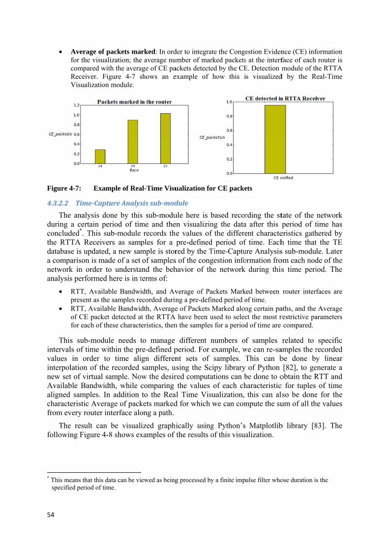
54
•
Figure 4
4.3.2.2 The
during concludthe RTTdatabasa companetworkanalysis
•
•
Thisintervalvalues interpolnew setAvailabaligned charactefrom ev
Thefollowin
* This me
specifie
Average of for the visuacompared wReceiver. FVisualization
4-7: Exa
Time-Cap
e analysis da certain p
ded*. This sTA Receiv
se is updatedarison is mak in order s performedRTT, Availapresent as thRTT, Availaof CE packefor each of t
s sub-moduls of time win order t
lation of tht of virtual ble Bandwid
samples. Ieristic Aver
very router i
e result canng Figure 4
eans that this ded period of ti
packets maalization; the
with the averaFigure 4-7 sn module.
mple of Rea
pture Analys
done by thisperiod of timsub-modulevers as samd, a new samade of a set to understa
d here is in table Bandwi
he samples reable Bandwiet detected athese charact
ule needs twithin the prto time alie recorded sample. Nodth, while In addition rage of packinterface alo
n be visual4-8 shows ex
data can be viime.
arked: In orde average nuage of CE pashows an e
al-Time Visu
sis sub-mod
s sub-modume and the
records thples for ample is storof samples
and the behterms of: idth, and Avecorded durindth, Average
at the RTTA teristics, then
to manage re-defined pign differensamples, u
ow the desircomparing to the Rea
kets markedong a path.
ized graphixamples of
iewed as being
der to integraumber of marackets detecteexample of
ualization fo
dule
ule here is ben visualizine values ofpre-definedred by the Ts of the conghavior of th
verage of Pang a pre-defie of Packets have been u
n the samples
different nperiod. For nt sets of
using the Scred computathe values
al Time Visd for which
ically usingthe results o
g processed by
ate the Congerked packetsed by the CEhow this i
or CE packe
based recorng the dataf the differed period of Time-Captugestion infohe network
ackets Markined period oMarked alon
used to selecs for a period
numbers ofexample, wsamples. T
cipy library ations can bof each ch
sualization, we can com
g Python’sof this visua
y a finite impu
estion Eviden at the interf
E. Detection ms visualized
ets
rding the sta after this ent charactef time. Eachure Analysisormation fro
during this
ed between of time. ng certain pact the most rd of time are
f samples we can re-saThis can bof Python
be done to oharacteristic
this can almpute the su
Matplotlibalization.
ulse filter who
nce (CE) infface of each module of th
d by the R
tate of the period of t
eristics gathh time thats sub-modulom each nods time peri
router interf
aths, and the restrictive pa compared.
related to amples the rbe done by[82], to ge
obtain the Rc for tuples lso be doneum of all th
b library [8
ose duration is
formation router is
he RTTA eal-Time
network time has hered by the TE le. Later de of the iod. The
faces are
Average arameters
specific recorded y linear
enerate a RTT and
of time e for the he values
83]. The
s the

Figure 4
Thisconditioas functbased oshould h
4.4 CIn th
has beeMany isacquire implemsome omeasuri
Furtfor undbottleneand pattest-bed
4-8: Tim
s implemeons in ordertion of time
on the Real-help is to un
Conclusihis chapter,en describedssues have b
data to mentation is of the proping RTT, ha
thermore, thderstanding ecks within ths). The ned in order to
me-Capture V
entation allr to verify te. In this w-Time Visunderstand th
on of th, an implemd along witbeen discushow to dconsistent
posed solutave been dis
his test-bed the behaviothe network
ext chapter o illustrate th
Visualization
lows usestrends and w
way, it is poalization fuhe behavior
his implementation inth details ossed rangingdeploy the
with the ptions descriscarded for
provides uor of the nek (hence wedescribes e
he convenie
n of the inte
to performwatch the d
ossible to counctionality.r of the netw
ementatn a test-bed of how eachg from selec
functionalproposed Coibed in thethis implem
us with the eetwork. Thise have focuexamples oence of this
erfaces of th
m simulatidistribution ontrast the c. The Time-
work over ti
tion chaof the Con
h of the mocting the aplity in theongestion-Ie design, smentation.
expected infs informatio
used on the lof characteri
method via
e RTTA Ro
ions with of the cong
consequenc-Capture Anme.
apter gestion-Ideodules has bppropriate tee network. dentificatiosuch as TC
formation inon should blimiting chaizations of a some use c
outer of the V
different gestion infoces of actionnalysis sub
entification been imple
echnical me In additi
on design; aCP Timesta
n a manner be useful to aracteristicsthe networ
cases.
55
VM-32
network ormation ns taken -module
scenario emented. ethods to ion, the although amp for
suitable identify of links
rk in the


57
5 Verification of the results Following an explanation of the design and the implementation, this chapter verifies a
mechanism for identifying congestion in a radio access transport network. The proposed solution is illustrated with two scenarios that confirm the functioning of the methods presented in this thesis. In these two examples, using the visualization tools implemented, the interaction between ECN and the OSPF-TE is monitored and access to the congestion information is confirmed.
Scenarios with different characteristics are compared to demonstrate the statements made in the previous paragraph. The details of these scenarios have been chosen to provide a clear visualization of the information provided and make the comparison of the state of the network easier for the reader. Different scenarios with different characteristics can be deployed to confirm that the features proposed in this thesis work as expected. In order to provide a verification of the results, the proposed scenarios are justified (to ensure that they are relevant and cover the most interesting and common cases of the network).
5.1 Congestion Emulation Tools The simulation of the congestion characteristics has required implementing in the test bed
different tools and devices. These tools are summarized in Table 5-1. These mechanisms provide the necessary features to characterize congestion in a network. Table 5-1: Tools used for Congestion Emulation and Simulation
IPERF Iperf [84] is a tool that can be used to perform network throughput measurements. To perform an Iperf test the user must establish both a server (to discard traffic) and a client (to generate traffic). The network performance measurement is done by loading the network in order to reach its limits (saturating the bottlenecks) without identifying the bottlenecks. For example, Iperf can inject TCP traffic in the network until the total available bandwidth is reached.
Portable Wide Area Network (WAN) Emulator
Linktropy Mini2 [85] is a device that can be configured to introduce congestion characteristics into a network. Connecting this equipment between two nodes, allows us to limit the bandwidth, increase the latency and jitter, and induce losses, thus emulating a congested link.
VLC Media Player VLC [86] is used to introduce user data traffic into the test-bed, specifically downloading streaming video via the RAN. The VLC media player encodes and streams video using different CODECs and formats. The video CODEC used in these experiments is H.264 and the audio codec is MP3 [87]. This choice of CODECs was convenient for the scenario, but other CODECs could have been used to provide a streaming media source. However, consideration of others CODECs is outside the scope of this thesis project. The protocol used for the streaming is UDP, this enable us to distinguish which video stream is suffering congestion. UDP was used due to its connection-less characteristic, thus avoiding the head of queue blocking that TCP would introduce when frames are lost.
VirtualBox The VirtualBox [65] virtualization software was not only used to deploy virtual machines in the test-bed equipment, it also allows characterizing of the internal guest links. With this option the bandwidth of the links can be limited and consequently, this allows modeling the link as if a specified portion of the bandwidth was reserved thus simulating that this amount of bandwidth is being used by other traffic.

58
The tools described in the table allow us to introduce different congestion circumstances that can be used to characterize and simulate different scenarios. Data from tests of these different scenarios enable us to explain and verify our results using visualization (see section 5.3.1).
5.2 Description of the different scenarios To illustrate the proposed mechanism; two different scenarios have been selected. These
scenarios are described in this section. Each of them utilizes specific traffic conditions in the test-bed in order to characterize the state of the links (in terms of latencies and bandwidths), and to influence marking actions in the routers. The first scenario, called the Congestion-less scenario, characterizes a network without bottlenecks or congestion. The second, the Congestion scenario, induces congestion in some parts of the network.
Some parts of the configuration of the network are the same in both scenarios. The evaluation of the mechanism with different configurations of these parameters remains for future work. The configuration used in these parameters, using the notation used in Chapter 4, follows:
• RED configuration of the router interface queues: The values chosen for the three different thresholds and the indicated probability allow the router interfaces to mark packets in case of congestion. This configuration is the same for each output queue of every router interface in the test-bed. Table 5-2 shows the values set.
Table 5-2: RED queues configuration
Minimum 1 Kbit
Maximum 2 Kbits
Limit of the queue 1.46 Mbits
Probability 60 %
• RTTA Router policies: The values set for deciding when to report congestion information from the RTTA Routers were set to obtain information from the routers in both scenarios. It is important to mention here, that the policies in the RTTA Routers were selected to allow us to save resources and minimize the volume of congestion information traffic - thus avoiding redundancy across the network [88]. Therefore, additional implementations that study how to configure the RTTA Router policies are needed, as will be described in the section 6.2. This router policies were chosen as described in Table 5-3.
Table 5-3: RTTA Router policies configuration
Database Read Interval 5 seconds
Threshold 10 %
Periodic update policy 100 seconds

In tNetworlocated;shown iare situtest-bedto it. EasituatedResults
• User trto simucongestthat twicons inPDN-Gconfigu
the charactrk comprise; as shown in Figure 5-ated in the P
d. Each RTTach RTTA Rd. In both sc
could be ob
raffic: User ulate user ttion as wello UEs belon the eNod
GW, using uration of th
Tabl
Video
Audio
terization oes the links
in Figure -1, in orderPDN-GW, TA ReceiveReceiver alscenarios, thebtained in a
traffic is crtraffic passil as to asseonging to e
desB of Figan applica
hese two VLe 5-4: V
o Bitrate
o Bitrate
of the test-and nodes w5-1. There to obtain r
eNode1 (eNer collects Oso detects Ce results ob
a similar fas
Figure
rossing the ning throughess the achieNode1 and
gure 5-1) aration such LC streaminVLC streami
-bed presenwhere the Rare three R
results in a rN1), and in OSPF-TE inCE marked pbtained are fshion from t
5-1: Sce
network froh the netwoieved QoE. d eNode2 rre downloadas VLC.
ng connectioing configur
1000 Mbps
448 Kbps
nted here, RTTA RoutRTTA Recerealistic scean eNode2
nformation fpackets comfrom the RTthe other tw
enario A
om the Interork and to
For this purespectivelyding a videTable 5-4
ons. ration
s
s
the Radio ters (A, B, Ceivers in thenario. Thes(eN2) that cfrom the RT
ming across TTA Receiv
wo RTTA Re
rnet to UEs study evid
urpose, we y (notice theo from beh
shows the
Access TC, D, E, an
he network,se RTTA Rcan be addeTTA Router the link whver situatedeceivers.
59
in order dence of
assume he video hind the e traffic
Transport nd F) are , as it is
Receivers ed to the r closest here it is
d in eN1.

60
5.2.1 Scenario A: Congestion-less network The results shown in this scenario are intended to show how the implemented mechanism
works in a RATN free of congestion. The information that has been gathered is presented in order to understand the state of the network and to compare this state with the results obtained in the Congestion scenario. In the Congestion–less scenario no congestion emulation tool was used and only the desired user traffic is added. The properties observed here describe the state of the network defined by the hardware and software characteristics described in section 4.1. This scenario formed the basis for the Scenario B, which includes additional equipment that will be used to characterize the state of the network when congestion is induced.
5.2.2 Scenario B: Congested path in the network This scenario simulates a RATN with congestion problems in one of its paths. Here, the
links of a specific path, {A, B, D}, cause bottlenecks resulting in traffic problems due to the introduction of congestion (via the emulation tools). The sources of congestion introduced are the following:
• The Portable WAN Emulator is situated in the link AB, introduces delays of 2 seconds for all of the packets crossing the link in either the uplink or downlink direction.
• The Virtual Box Link Characterization is located in the link BD, emulating an existing bandwidth utilization of 950 Mbps for this link.
• An Iperf connection is established to load the whole {A, B, D} path in order to force the marking of packets.
These three modifications of the traffic conditions imitate circumstances that can actually occur in an LTE network, due to different factors as described in the introduction. Figure 5-2 illustrates Scenario B. This figure shows where the emulation tools have been placed, along with the congested paths and links.

In aScenaridifferenF}.
5.3 AIn t
networkboth Re
Thepaths. Hof the pgatherecongestThe patsimulatconclusthe endevent of
5.3.1
In tgraphicmonitor
addition, asio A is depnce in QoE
Analysisthis section,k conditionseal-Time Vi
e comparisoHowever, foproposed med and anation informaths studiede realistic
sions regardd of this chf congestion
Real Timthis section cal presentaring data at
s describedployed herprovided to
of the r, the resultss of both scisualization
ons could hor the purpoechanism. F
alyzed. For ation is bein
d are {A, BRATN wit
ding what fuhapter, whern.
e Visualiza real-time
ation of thet a certain m
Figure
d before, the, includino a UE con
resultss obtained
cenarios by and Time-C
have been dose of this thFor this rea
each of tng analyzed
B, D}, {A, thin a LTEurther actionre we study
zation e comparisoe results vmoment; ho
5-2: Sce
he same cong the usernnected via
from both performingCapture.
done by selhesis projecson a relevathe two vi
d, along withC, F}, and
E network. ns should bey potential
on betweenvisualized inowever, the
enario B
onfigurationtraffic –
different p
scenarios ag the analysi
ecting sevect we are coant selectioisualization h which patd {D, F}; a
The resulte taken. Thealternatives
n the scenarn real timetool actuall
n of the neso that weaths, i.e. {A
are analyzedis proposed
eral router ioncerned abn of conges
methods ths have beeas these pats of this aese actions ws that could
rios is donee are showly shows th
etwork as e can compA, B, D} or
d. We compd in Chapter
interfaces, lbout the verstion informwe explainen chosen aaths allowinanalysis shwill be discd be utilize
e. In this thwn based uhe data in re
61
used in pare the r {A, C,
pare the r 4 using
links, or ification
mation is n which and why. ng us to hould be cussed at d in the
hesis the upon the eal-time.

62
The twocharactesection or used network
Fromexperiensnapshopresentstransporstandardbetweenuser. Alink fram
o scenarios eristics are 5.3.2. This in real-tim
k.
m an UE’s nces, for iots, the vides the visualrt path {Ad quality. In the eN1 a
As one can emes.
are presentthe same. visualizatio
e in order f
point of vieinstance, ineo experienlization of , C, F} is In contrast, and the PDNeasily see th
Figure 5-
Figure 5-
ted using baThis graph
on describefor a networ
ew, the conn the visuaces of the tthe video fnot congesFigure 5-4
N-GW {A, he video in
-3: Video
-4: Video
ar charts at hical limita
ed in this secrk operator t
ngested statealization otwo UEs in from a usersted, allow4 shows hoB, D} nega
n Figure 5-4
o seen by a U
o seen by a U
different mation of a pction providto react to t
e of the netwf a streamthe Scenari
r connectedwing the useow the congatively affec4 is degrade
UE connect
UE connect
moments of printed thesdes informathe congesti
work is reflming video.
io B are comd to an eNoer to watchgestion introcts the videoed by the e
ed to eN2
ed to eN1
time, but wsis is addre
ation to be aion occurrin
lected in the In the fompared. Fig
ode (eN2) wh the videooduced in to experienc
effects of m
when the essed in analyzed ng in the
e QoE it ollowing gure 5-3 when its o with a the path ce of the
many lost

In tconnectorganizand visu
5.3.1.1 The
routers a letter
RouFigure comparWAN eD0) toothan the
Avainformathat noprovidebeen rethe avatraffic i
the followited to eN1
zed by interualized prov
Per Route
e congestionof the netwand the num
und Trip T5-5, conge
rison betweeemulator in o. The intere others. No
Figure 5-5
Figure 5-6
ailable Banation for eaco bandwidthed by interfaeached (henailable link njected by t
ing subsectare displa
face and byvides inform
er Interface
n informatiowork. The bamber of the
Time: In thiestion-less en both scethe link AB
rfaces incluotice that the
5: Real T
6: Real T
ndwidth: ch of the dih is consum
faces B1 andnce there is
bandwidth the tools.
tion, the reyed with c
y path. Thesmation abou
e Analysis
on shown hear chart preinterface.
s study the scenario, anarios is pr
B (A1-B0) iuded in the e vertical sc
ime Visualiz
Time Visualiz
Figure 5-7fferent intermed by and D0 reflecno availablof the oth
easons forcomparisonsse comparisut the state o
ere correspoesents the in
RTT and thand the Firesented. Inis visualizedpath {A, B
cale is differ
zation of the
zation of the
7 and Figurfaces in th
ny interfacect the fact thle bandwid
her interface
the poor Qs of the disons verify of the netwo
onds to infonterfaces of
he availableigure 5-6 c
n these graphd and the li
B, D} preserent Figure
e RTT by In
e RTT by In
ure 5-8 she two scena
e, while inhat the bandth via thesees in the ne
QoE experifferent conthat the inf
ork in real ti
ormation cothe routers
e bandwidthcongested shs the delaymited cong
ent higher R5-5 than in
nterfaces in
nterfaces in
ow the avarios. In Fig
Figure 5-dwidth limie interfacesetwork refle
rienced by ngestion parformation ctime.
ollected from, each ident
h are studiedscenario, thy introduce
gested link BRTT measu
n Figure 5-6
Scenario A
Scenario B
vailable bagure 5-7 we-8, the infoitation of a s). The reduects the am
63
the UE rameters collected
m all the tified by
d. In the he RTT d by the BD (B1-urements .
andwidth e can see ormation link has
uction in mount of

64
Figure 5
Figure 5
Aveinto themechan
No there arScenariIn this output Figure traffic) packetsnumberreal-timpacketsand take
Figure 5
5-7: Rea
5-8: Rea
erage of pae visualizatnisms (ECN
bar charts re no markeio B. Figurecase, as wadownlink q5-10 showsat the end
s are the samr of CE pac
me visualizas marked), ne further ac
5-9: Reain S
l Time Visu
l Time Visu
ackets marktion, we pr
N and OSPF-
of Scenarioed packets e 5-9 showsas expectedqueue of ints the avera
d point of thme packets ackets acts asation of thenot only by ctions to solv
l Time Visucenario B
ualization of
ualization of
ked: In ordresent in re-TE) and ve
o A are shodetected atthe average
d, the only iterface B1
age numberhe ECN coas marked bs a “congese congestiopath, but byve the cong
ualization of
f the Availab
f the Availab
der to integreal-time theerify the res
own, since t the eNodee number ointerface thof the simu of CE pacommunicatiby the B1 instion experion parametey interface,
gestion prob
f the averag
ble Bandwid
ble Bandwid
rate the Cone interactiosults of this
due to its es. Both of f packets be
hat is markiulated congckets detection, in this nterface. Thienced” alarers (bandwthe networ
blems in the
e number o
dth by Interf
dth by Interf
ngestion Evon between interaction.
congestion-the followieing markedng packets
gested link. ted (as provcase, the e
e real-time rm for the nidth, latenck operator inetwork.
f packets m
faces in Scen
faces in Scen
vidence infothe propo
.
-less characing figures d by each incorrespondAt the sam
voked by teNode1. Thvisualizationetwork. Gcy, and numis now able
marked per I
nario A
nario B
ormation sed two
cteristics concern
nterface. ds to the me time, the Iperf hese CE on of the
Given the mber of
e to react
Interface

Figure 5
5.3.1.2 An
{A, C, introducbandwi
RoubetweenconsideB, D} iFigure A). In tpaths aFigure 5
5-10: Reaat eN
Per Path Aanalysis of F}, in ordection of thdth characte
und Trip Tn the sumsered. As shois higher tha5-11 showsthis case th
are equally 5-12.
l Time VisuN1
Analysis f different per to compahis section)eristics as p
Time: The ss of the mown in Figuan for the ps the corres
he sums alonloaded. No
ualization of
aths was peare the traff. The com
presented by
study of themost restricure 5-12 (copath {A, C, sponding Rng the two
otice that th
f the averag
erformed fofic condition
mparisons ay the Real T
e total RTTctive measuorresponding
F}, due to RTTs for the
paths are she vertical
ge number o
or two pathsns of both p
are done ofTime Visual
T along the urements og to Scenarithe conges
e congestiosimilar – whscale is dif
of CE mark
s of Figure paths (as wf the RTT ization func
paths consif the RTTio B), the Rtion implem
on-less scenhich is as efferent in F
ked packets
5-2 {A, B,was describe
and the actionality.
iders the diTs along thRTT of the pmented in thnario (i.e., Sexpected sinFigure 5-11
65
detected
D} and ed in the available
ifference he paths path {A, his path. Scenario nce both
than in

66
Figure 5
Figure 5
Avabandwilimited along thavailablFigure bottleneavailabl
5-11: Rea
5-12: Rea
ailable Bandth reflectsavailable b
hat path. File bandwidt5-14 easily
eck (due to le bandwidt
l Time Visu
l Time Visu
ndwidth: T the differebandwidth igure 5-13 th as expecty allows usthe BD lin
th of the pat
ualization of
ualization of
The comparinces betwecomputed correspondsted due the s to identif
nk) and verith.
f the RTT by
f the RTT by
ison of boten these twfrom the los to Scenarcongestion-
fy that the fies that it i
y Paths in th
y Paths in th
th scenarioswo paths. Heowest availrio A, wher-less characpath {A, B
is this bottl
he Scenario A
he Scenario B
s with regaere the visulable bandwe all the pateristics of tB, D} conteneck link
A
B
ard to the aualization shwidth measaths show ththis scenaritains the sithat limits
available hows the urement he same io, while imulated the total

Figu
Figu
5.3.2
As make apropose
OnceN1 expScenarivisualiz
Thedefiniteover timcould brouter in
ure 5-13: R
ure 5-14: R
Time-Capsame way
a comparisoed mechanis
ce again weperiences thio A, and mzations show
e analysis ise time periome. Howevbe chosen. Tnterface and
Real Time V
Real Time V
pture Anaas in the pr
on between sm to analy
e use two vihe same vidmuch worswed.
s done in teod was selecver, another The followid path (resp
Visualization
Visualization
alysis revious secthe Scenarze the state
deo streamsdeo quality e in the Sc
erms of roucted to guar
pre-definiting paragra
pectively).
n of the Ava
n of the Ava
ction on Rerio A and B
of the netw
s. During th as was obscenario B,
uter interfacrantee a steate period thaphs describ
ilable Bandw
ilable Bandw
al-Time ViB to illustrawork over a
he period observed for aas several
ces and pathady state ofhat satisfiesbe the resul
width by Pa
width by Pa
sualization,ate the resuperiod of ti
bserved, a Ua UE connetime frame
hs over 60 f the networ this steadylts obtained
ath in Scena
ath in Scena
, in this secults obtainedime.
UE connecteected to eNes in the r
minutes. Trk in both sy state requ
d in the ana
67
rio A
ario B
ction we d by the
ed to the N2 in the real-time
This pre-cenarios uirement alysis by
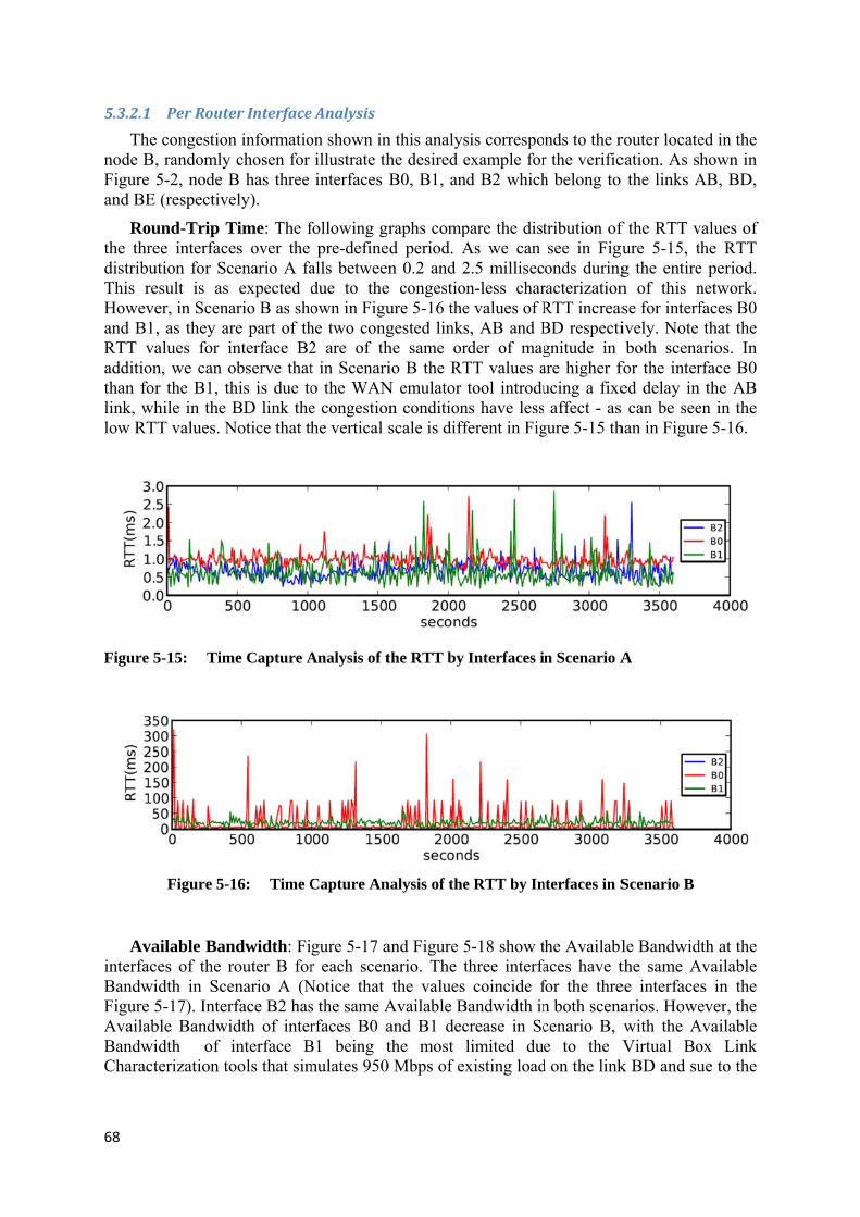
68
5.3.2.1 The
node B,Figure and BE
Routhe thredistribuThis reHoweveand B1RTT vaadditionthan forlink, whlow RT
Figure 5
AvainterfacBandwiFigure 5AvailabBandwiCharact
Per Route
e congestion, randomly 5-2, node B (respective
und-Trip Tee interfaceution for Scesult is as er, in Scena, as they aralues for inn, we can or the B1, thhile in the B
TT values. N
5-15: Tim
Figure 5-1
ailable Bances of the ridth in Sce5-17). Interble Bandwiidth of iterization to
er Interface
n informatiochosen for
B has three ely).
Time: The fes over the cenario A fa
expected dario B as shore part of thnterface B2
observe thathis is due toBD link the
Notice that th
me Capture A
16: Time C
ndwidth: Firouter B forenario A (Nface B2 hasdth of interinterface Bools that sim
e Analysis
on shown inillustrate thinterfaces B
following grpre-define
alls betweendue to theown in Figuhe two cong2 are of tht in Scenario the WANe congestionhe vertical s
Analysis of t
Capture An
gure 5-17 ar each scen
Notice that s the same Arfaces B0 a
B1 being tmulates 950
n this analyshe desired eB0, B1, an
raphs compd period. An 0.2 and 2
e congestionure 5-16 thegested linkshe same orio B the RT
N emulator n conditionscale is diff
the RTT by
nalysis of the
and Figure 5nario. The t
the values Available Band B1 decthe most l
0 Mbps of ex
sis correspoexample ford B2 which
pare the distAs we can 2.5 millisecn-less chare values of Rs, AB and Brder of magTT values atool introdu
ns have lessferent in Fig
Interfaces i
e RTT by In
5-18 show tthree interfa
coincide fBandwidth increase in Sclimited duxisting load
nds to the rr the verifich belong to
tribution of see in Figuonds during
racterizationRTT increasBD respectignitude in are higher fucing a fixe affect - as
gure 5-15 th
n Scenario A
nterfaces in S
the Availablaces have tfor the thren both scenacenario B, e to the V
d on the link
router locatecation. As s the links A
f the RTT vure 5-15, tg the entiren of this nse for interfively. Note both scena
for the intered delay in can be see
han in Figur
A
Scenario B
le Bandwidthe same Aee interfacearios. Howewith the AVirtual Bo
k BD and su
ed in the hown in
AB, BD,
values of the RTT e period. network. faces B0 that the
arios. In rface B0
the AB en in the re 5-16.
dth at the Available
s in the ever, the
Available ox Link ue to the

Iperf trinterfac
Figur
Figure 5
AveCaptureinterfacin the Sinterfacqueues that expsimulatIperf anthe linkare not and thedelays wno traff
Figure 5
raffic crossice B0 decrea
re 5-17: Tim
5-18: Tim
erage nume Analysis ce. The FiguScenario B.ces is 0 durof the route
periences hiion of 950
nd user traffk AB introdaccumulati
ere is still swaiting for fic problem
5-19: Time Scen
ing the patases by roug
me Capture A
me Capture A
ber of Mafunctionalit
ure 5-19 sho In the Scering the enter do not exigh load of Mbps of ex
fic crossingducing delaying in the ousufficient avtransmissiofor the link
Capture Annario B
th {A,B,D}ghly 50 Mb
Analysis of t
Analysis of t
arked Packty is the avows these venario A, thtire period, xperience anits output q
xisting bandg the path {Ay, no packeutput queuevailable outon. Therefork BE.
nalysis of the
}. In Scenabps, due to t
the Availabl
the Availabl
kets: The fverage num
values for thhe Average
as the trafany significaqueue is thedwidth beinA, B, D}. Hets are marke of the intetgoing bandre, interface
e Average N
ario B the the Iperf tra
le Bandwidt
le Bandwidt
final paramember of marhe three inte
Number offfic in the nant load. In e interface Bng used forHowever, evked at the ierface, as thdwidth; howe B2 does n
Number of M
Available ffic on the l
h by Interfa
th by Interfa
eter analyzerked packet
erfaces durinf Marked Pnetwork is scenario B
B1. This occthe link BD
ven with thenterface B0
he communiwever, thesenot mark pa
Marked Pac
Bandwidth link AB.
aces in Scen
aces in Scen
ed with outs sorted bng the entir
Packets for really low
B, the only icurs becausD together e WAN emu0, since the nication is de packers dackets since
ckets by Inte
69
for the
ario A
ario B
ur Time-y router
re period all three and the
interface se of the with the ulator in packets
downlink do suffer e there is
erface in
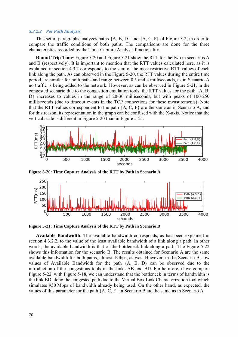
70
5.3.2.2 This
comparcharacte
Rouand B (explainlink aloperiod ano traffcongestD} incrmillisecthat thefor this vertical
Figure 5
Figure 5
Avasection words, shows tavailablvalues introducFigure 5the linksimulatvalues o
Per Path As set of parare the trafferistics reco
und-Trip T(respectiveled in sectio
ong the pathare similar fic is being ted scenarioreases to vconds (due e RTT value
reason, its rl scale is dif
5-20: Time C
5-21: Time C
ailable Ban4.3.2.2, to the availabthis informale bandwidtof Availab
ction of the5-22 with F
k BD along tes 950 Mbpof this param
Analysis agraphs anafic conditioorded by the
Time: Figurey). It is imp
on 4.3.2 corh. As can obfor both patadded to th
o due to the values in thto timeout
es corresponrepresentatifferent in Fi
Capture An
Capture An
ndwidth: Tthe value o
ble bandwidation for thth for both ble Bandwie congestionFigure 5-18the congestps of bandwmeter for th
alyzes pathsons of bothe Time-Cap
e 5-20 and Fportant to mrresponds tobserved in thths and rang
he network. congestion
he range oevents in tndent to theion in the grigure 5-20 th
alysis of the
alysis of the
he availablof the leastdth is that oe scenario Bpaths, almoidth for thns tools in , we can un
ted path duewidth alreadhe path {A,
s {A, B, D}h paths. Thpture Analys
Figure 5-21mention thao the sum ohe Figure 5-ge between However,
n emulation of 20-30 mthe TCP coe path {A, Craph can behan in Figu
e RTT by Pa
e RTT by Pa
le bandwidtavailable b
of the bottleB. The resuost 1Gbps, he path {A
the links Anderstand the to the Virtdy being usC, F} in Sc
} and {A, Che comparisis function
1 show the Rat the RTT vf the most r-20, the RTT
n 0.5 and 4 mas can be otools, the R
milliseconds,nnections fC, F} are th
e confused wure 5-21.
ath in Scena
ath in Scena
th corresponbandwidth oeneck link aults obtainedas was. Ho
A, B, D} cAB and BDhat the bottletual Box Linsed. On theenario B ar
C, F} of Figisons are dality.
RTT for thevalues calcurestrictive RT values dumillisecond
observed in RTT values , but with for these mehe same as with the X-a
ario A
ario B
nds, as hasof a link aloalong a pathd for Scenawever, in thcan be obs
D. Furthermoeneck in ternk Charactee other hane the same a
gure 5-2, in done for th
e two in scenulated hereRTT valuesuring the entds, as in Sce
Figure 5-2for the pathpeaks of
easurementin Scenario
axis. Notice
s been explong a path. h. The Figu
ario A are the Scenarioserved dueore, if we crms of banderization toond, as expecas in Scena
order to he three
narios A , as it is of each tire time enario A 1, in the h {A, B, 100-250 ts). Note o A, and e that the
ained in In other ure 5-22 he same o B, low e to the compare
dwidth is ol which cted, the rio A.

Figure 5
Avemarkeddetectedmarkedthe figuScenarivalue rathe avecomparof Packinterfactraffic aPackets
Figure
5-22: Time C
erage numbd packets fod in the RT
d on any pature coincideio B, it cananging in vrage numbe
ring the Figukets Markedce B1, sinceare downlins for the path
5-23: TimeDete
Capture An
ber of maror the two pTA Receiveths and no Ce during thn be observalue betweeer of markeure 5-23 wid in the pae the link Bnk through h {A, C, F}
e Capture Aected by Pat
alysis of the
rked packepaths and ther (located iCE packets he entire peved that theen 0-8 packed packets dith the Figuath {A, B, BD is loade
this link. O} has the sam
Analysis of th in Scenar
e Available B
ets: The Fighe Average in the eN1)has been de
eriod of time Average Nkets markeddetected at
ure 5-19, it cD} almost
ed with 950On the otheme behavior
f the Averario B
Bandwidth b
gure 5-23 sNumber of. In the Sceetected at eN
me), as no cNumber of
d per secondeN1 is sim
can be obset coincides0 Mbps of ter hand, ther in both sc
age of Num
by Paths in
shows the Af Congestionenario A, noN1 (note thcongestion tf Marked Pds for the {A
milar for thirved that thwith the s
raffic and be Average Nenarios.
mber Marke
the Scenari
Average nun Evidence o packets hahat the threetraffic is adackets incrA, B, D} ps path. In a
he Average same paramboth Iperf aNumber of
ed Packets
71
o B
umber of packets
ave been e lines of dded. In reases in path; and addition, Number
meter for and user Marked
and CE

72
5.4 Conclusion of the Verification of the Results The study of the two scenarios has confirmed that we have achieved the main goals of
this thesis project. Scenario A considers the initial network without congestion and traffic, while Scenario B purposely introduces congestion, specifically introducing congestion along one of the paths between eN1 and the gateway; while the path between the eN2 and the gateway does not suffer congestion.
A real-time study has been conducted to monitor the state of the network in two scenarios. In Scenario B, the consequences from the UE’s point of view are that it suffers due to the congestion happening on the path through the RATN. Moreover, these real-time results have been corroborated with an analysis of the congestion information done for a long period of time. In the Appendix B is given a complete visualization for the scenarios proposed.
In addition, the Scenario B illustrates the difference between the QoE of a video that two UEs, connected to two different eNodeBs, will experience. This difference is supported by the study of the links’ congestion parameters (available bandwidth, RTT, and number of ECN marked packets) and their interaction with the CE evidence observed at eN1. This analysis demonstrates that the RTTA Router in the links of the congested path, and specifically the one which is the objective of the most restrictive congestion emulation features, provide more critical measurements of these parameters compared with those supplied by an RTTA Router of the other path. At the same time, the observation of these parameters in the eN1 corroborates the information concerning the evidence of congestion in the network, as provided by the detection of CE packets done by the RTTA Receiver in the eN1.
As it has been shown in this case study, the implementation of the proposed mechanism allows us to obtain information about the state of the links of the network. With the information gathered and processed by the RTTA Receiver, further actions can be proposed in order to improve the QoE of the UE connected to the eNodeB whose path to the gateway is congested. These actions could imply a handover of the UE to another eNodeB (if this eNodeB is close enough) or balancing the load between these two base stations. The combination of these visualization methods that have been implemented, confirm that: The interaction of the two proposed mechanisms provides relevant traffic information and consequently helps to identify congestion in a RAN.

73
6 Conclusions and Future work This chapter describes a general conclusion based upon the work done during this thesis
project and provides suggestions for next steps in order to continue the work. The intention of this chapter is to point out the most relevant ideas of the thesis and then consider how to build upon them in future research.
6.1 Conclusions The mechanism proposed in this thesis project gives a solution that can be used to
identify congestion in a Radio Access Transport Network. This thesis has described, discussed, and verified in a test-bed the proposed mechanism, giving a complete framework that supports it for continuing working on it or even deploying it into real networks. Taking into account the sub-goals stated in section 1.3, they can be divided into two: (1) “investigate protocols related to congestion control and the interaction between these protocols” and (2) “propose a mechanism that identifies congestion in a radio access transport network”. Having divided them in this way several reflections may be made:
• The investigation of previous work allowed us to comprehend the scenario central to this thesis project, enabling us to detect and understand the most important relevant concepts. The study of mobile networks, in particular, understanding the RATN and its interaction with other parts of the network, guided us to focus on the RATN it the next steps of the project. This lead to research concerning the ECN and OSPF-TE protocols and how these might help us locate the congestion and then exploit the congestion control protocols operating in the RATN. The study of the interaction of these protocols and the consideration of new concepts, such as I2RS, leaded us to the design the proposed new mechanism.
• The design, implementation, and verification of the proposed mechanism address the second sub-goal of the thesis. Although, many issues can be discussed as part of an effort to optimize the mechanism proposed here. Some of these issues are related to the reliability of the mechanism when measuring the congestion information (as was discussed in section 3.2.1.1 concerning the design and in section 4.2.1 concerning the implementation). In addition, if we could travel back in the time, we would have focused on optimizing the policies regarding forwarding or not forwarding certain congestion information, and from an implementation point of view, we would have placed more attention on the efficiency of the code that we have developed.
As a result of the above reflections, the next section proposes new actions that could be undertaken in order to improve the proposed solution.
We conclude this thesis with a summary of some of the personal achievements of the authors during the project. This thesis project has given us a greater understanding of mobile networks, particularly of the interaction of the Radio Access Transport Network with the Radio Access part and the protocols used therein, learning new programming languages (Bash, Python), and improving our command of C programming language and Linux environment. We are especially thankful for the knowledge that we have gained about network configuration and traffic control. Moreover, carrying out this thesis project has improved the authors skills related to solving problems, carrying out a large project, and working as part of a team.

74
6.2 Future work Following the description of the work done during this Master’s thesis project, we have a
number of different suggestions about work that could follow and build upon our research. This future can be mainly divided into two areas: (1) research and discussion focused on improving the design and implementation and (2) the exploitation of the possibilities and ideas that have been introduced throughout the thesis. In the paragraphs below we summarize the proposed future work.
The first direction for proposed additional research is the study and use of protocols other than those described here. The research would focus on the features that these other protocols provide that could be used to obtain the required information. In this thesis the ECN protocol has only considered the case of IPv4, hence an interesting related effort would be an implementation of the proposed mechanism for IPv6, following RFC 3168 [13] and the work done by the KAME project [89]. Some of the other possible protocol options that could be considered and studied are MPLS-TE [27], IGRP-DUAL [57], and IS-IS [90]. These protocols provided similar traffic engineering features to those provided by OSPF-TE (OSPF-TE is even part of MPLS-TE), hence these protocols could be used to distribute routing and congestion information throughout the network. Together with this research, a very interesting extension of the work here presented would be the distribution of the traffic engineering information between different areas or ASs, for example by utilizing inter-domain routing protocols such as BGP [91].
The next area for potential future research is implementing and performing the traffic measurements via the RTTA Router. During this thesis, the focus was finding a suitable way to extract the desired parameters via a simple implementation in our test-bed. We have not focus on their accuracy. Therefore an obvious area of future research is to improve the quality of these measurements. For example, in the case of the available bandwidth parameter, deeper research should be undertaken to estimate the total available bandwidth. As was explained in the section 4.2.1.2 the measurement of the one-way delay had to be excluded from this thesis project due to the low synchronization accuracy provided by NTP alone. However, by deploying PTP [73] in the network, this parameter could be accurately and reliably measured, providing more precise information about the state of the links. Finally, the configuration of the output queue of the routers interface that was deployed did not follow any standard or recommended model, rather the aim was simply to provide evidence of packets being marked within the network. Once this evidence has been verified, a following step may be an investigation comparing different AQM configurations together with a complete study in order to provide the most suitable characterizations of these queues. Moreover, the software developed during the thesis project sometimes lacks efficiency and some sections and modules could be improved to achieve better performance.
In conjunction with section 3.2.2, relevant future research could be done about what policies should be followed in order to control the flooding of the traffic, for example building upon the work presented by Roozbeh in his thesis [53]. However for the case considered in our study, a complete investigation of more suitable updating policies could provide information relevant to improving the efficiency of the distribution of the congestion information. At the same time, this study could be combined with a deeper analysis of different simulated scenarios. In section 5.2, two different characteristic scenarios were proposed and monitored in order to verify the proposed solution. In addition to these two scenarios, more complex simulations can be performed, for example by changing the configuration of the traffic parameters and adding more tools to characterize the network in

75
different ways. This analysis could provide a more complete verification and analysis to support the usage of the proposed mechanism.
In this master thesis, access to the information from the routing system has been designed according to the idea proposed in the I2RS draft document [92]. While the implemented approach provides important features of this interface, future work future work could extend this both for our proposed solution and also for other network systems.
Finally, the mechanism proposed in this thesis is just the beginning of future work that could be done in order to solve (or avoid) congestion problems in a RATN. Once the first step identify where exactly the congestion is happening, is completed; then the next steps should focus reactions to this congestion in order to ensure the expected QoE. For instance, future research could study the impact of this proposed solution on the decision that an eNodeB with UEs connected to it (that is aware of the existence of congestion in its path to internet and has identified this congestion) can take; for example, to perform a handover to another eNodeB that is aware that its path is not congested. Another possible direction is to study load balancing between different eNodeBs and how the user’s IP tunnels between the PDN-GW and the UE’s current eNodeB should be modified.
6.3 Required reflections This section discusses the social, economic, and sustainability aspects of deploying the
congestion identification mechanism proposed in this master thesis project in Radio Access Transport Networks. The deployment of this mechanism enables mobile networks operators to take actions in order to provide the expected quality of experience to their users. This effect should drive mobile networks operators to procure the promised services, increasing the client satisfaction which is a desirable social effect of this master thesis project.
Moreover, the implementation of the mechanism described in this thesis, does not need any change in the current network architecture and any new element has to be included. Just an extension of the existing elements in the RATN allows providing the features described in this report. This implies a relevant economic issue to the operators involved in the deployment of the network because this enhancement does not require any extra economic cost. In addition, the real time reaction that this mechanism provides in order to exactly identify the congested link in the network, allows to the mobile network operators to decrease the cost related to solve network congestion problems, which is an important economic benefit of this work.
Furthermore, the knowledge of the state of the network allows the properly use of the existing resources and avoid that mobile network operators invest in extra equipment to provide the expected quality of experience to the users. This reduction in terms of investing in resources and equipment implies a more sustainable solution in mobile networks.


77
Bibliography [1] “ITU Statistics,” ITU. [Online]. Available: http://www.itu.int/en/ITU-
D/Statistics/Pages/stat/default.aspx. [Accessed: 19-Sep-2013]. [2] Cisco, “Cisco Visual Networking Index: Global Mobile Data Traffic Forecast Update, 2012–
2017.” Cisco Systems, Inc. [Online]. Available: http://www.cisco.com/en/US/solutions/collateral/ns341/ns525/ns537/ns705/ns827/white_paper_c11-520862.pdf.
[3] Ericsson, “Ericsson predicts Mobile Data Traffic to grow 10-fold by 2016,” 07-Nov-2011. [Online]. Available: http://www.ericsson.com/news/1561267. [Accessed: 19-Sep-2013].
[4] Cisco, “Evolution of the Mobile Network.” White paper, Cisco Systems, Inc., C11-624446-00, October 2010 [Online]. Available: http://www.cisco.com/c/en/us/solutions/collateral/service-provider/mobile-internet/white_paper_c11-624446.pdf. [Accessed: 19-Sep-2013].
[5] 3GPP, “3GPP Scope and Objectives.” [Online]. Available: http://www.3gpp.org/ftp/Inbox/2008_web_files/3GPP_Scopeando310807.pdf.
[6] “Mapping LTE Deployments: LteMaps.” [Online]. Available: http://ltemaps.org/home/. [Accessed: 19-Sep-2013].
[7] M. Olsson, S. Sultana, S. Rommer, L. Frid, and C. Mulligan, SAE and the Evolved Packet Core: Driving the Mobile Broadband Revolution, 2009. Academic Press.
[8] T. Senathirajah, “Smart Network Towards Better Quality Of Experience (QoE).” [Online]. Available: http://myconvergence.com.my/main/images/stories/PDF_Folder/july2011/MyCv08_pg52_57_SmartNetwork_low.pdf.
[9] B. E. Carpenter and C. Partridge, “Internet requests for comments (RFCs) as scholarly publications,” SIGCOMM Computer Communication Review, vol. 40, no. 1, pp. 31–33, Jan. 2010.
[10] P. Fuller, “LTE MAC Scheduler and Radio Bearer QoS.” Roke Manor Research Ltd, 2001. Available: http://www.roke.co.uk/resources/white-papers/0485-LTE-Radio-Bearer-QoS.pdf
[11] M. Sauter, From GSM to LTE: An Introduction to mobile networks and mobile broadband., 2011, Wiley.
[12] 3GPP, Evolved Universal Terrestrial Radio Access Network. (E-UTRAN): “S1 Application Protocol (S1AP)(Release 10),” 2011.
[13] K. Ramakrishnan, S. Floyd, and D. Black, “The Addition of Explicit Congestion Notification (ECN) to IP,” Internet Request for Comments, RFC 3168 (Proposed Standard), Sep. 2001.
[14] J. Heinanen, “Use of the IPv4 TOS Octet to Support Differential Services.” November 1997, Expired May 1998 [Online]. Available: http://tools.ietf.org/html/draft-heinanen-diff-tos-octet-01. [Accessed: 14-Oct-2013].
[15] D. Pacifico, M. Pacifico, C. Fischione, H. Hjalrmasson, and K. H. Johansson, “Improving TCP performance during the intra LTE handover,” in Global Telecommunications Conference, 2009. GLOBECOM 2009. IEEE, 2009, pp. 1–8.
[16] Ericsson, “Identify bottleneck in RAN transport and avoid congestion with optimized radio and network usages,” P10259PC00;01-Mar-2013.
[17] J. Moy, “OSPF Version 2,” Internet Request for Comments, RFC 2328 (Internet Standard), Apr. 1998.
[18] E. W. Dijkstra, “A note on two problems in connexion with graphs,” Numer. Math., vol. 1, no. 1, pp. 269–271, Dec. 1959.
[19] J. Moy, “OSPF: Anatomy of an Internet Routing Protocol,” in OSPF: Anatomy of an Internet Routing Protocol, pp. 71–99.
[20] B. Fenner and K. Kompella, “IANA Considerations for OSPF.” Internet Request for Comments, RFC 4940 (Best Current Practice), July 2007, Available at http://www.rfc-editor.org/rfc/rfc4940.txt. [[Accessed: 12-Sep-2013].
[21] L. Berger, I. Bryskin, A. Zinin, and R. Coltun, “The OSPF Opaque LSA Option,” Internet Request for Comments, RFC 5250 (Proposed Standard), July 2008.

78
[22] Internet Assigned Numbers Authority (IANA), “Open Shortest Path First (OSPF) Opaque Link-State Advertisements (LSA) Option Types.” Last updated 2009-01-07 [Online]. Available: http://www.iana.org/assignments/ospf-opaque-types/ospf-opaque-types.xml. [Accessed: 12-Sep-2013].
[23] D. Katz, K. Kompella, and D. Yeung, “Traffic Engineering (TE) Extensions to OSPF Version 2,” Internet Request for Comments, RFC 3630 (Proposed Standard), Sep. 2003.
[24] J. Moy, P. Pillay-Esnault, and A. Lindem, “Graceful OSPF Restart,” Internet Request for Comments, RFC 3623 (Proposed Standard), Nov. 2003.
[25] A. Lindem, N. Shen, J. Vasseur, R. Aggarwal, and S. Shaffer, “Extensions to OSPF for Advertising Optional Router Capabilities,” Internet Request for Comments, RFC 4970 (Proposed Standard), July 2007.
[26] I. Bryskin and L. Berger, “OSPF-Based Layer 1 VPN Auto-Discovery,” Internet Request for Comments, RFC 5252 (Proposed Standard), July 2008.
[27] M. Chen, R. Zhang, and X. Duan, “OSPF Extensions in Support of Inter-Autonomous System (AS) MPLS and GMPLS Traffic Engineering,” Internet Request for Comments, RFC 5392 (Proposed Standard), Jan. 2009.
[28] Internet Assigned Numbers Authority (IANA), “Open Shortest Path First (OSPF) Traffic Engineering TLVs.” Last updated 2013-12-16 [Online]. Available: http://www.iana.org/assignments/ospf-traffic-eng-tlvs/ospf-traffic-eng-tlvs.txt. [Accessed: 12-Sep-2013].
[29] K. Ishiguro, V. Manral, A. Davey, and A. Lindem, “Traffic Engineering Extensions to OSPF Version 3,” Internet Request for Comments, vol. RFC 5329 (Proposed Standard), Sep. 2008.
[30] K. Kompella and Y. Rekhter, “OSPF Extensions in Support of Generalized Multi-Protocol Label Switching (GMPLS),” Internet Request for Comments, RFC 4203 (Proposed Standard), Oct. 2005.
[31] R. Aggarwal and K. Kompella, “Advertising a Router’s Local Addresses in OSPF Traffic Engineering (TE) Extensions,” Internet Request for Comments, RFC 5786 (Proposed Standard), Mar. 2010.
[32] Internet Assigned Numbers Authority (IANA), “Open Shortest Path First (OSPF) Traffic Engineering TLVs.” Last updated 2013-12-16 [Online]. Available: http://www.iana.org/assignments/ospf-traffic-eng-tlvs/ospf-traffic-eng-tlvs.txt. [Accessed: 12-Sep-2013].
[33] A. Malis, A. Lindem, and D. Papadimitriou, “Automatically Switched Optical Network (ASON) Routing for OSPFv2 Protocols,” Internet Request for Comments, RFC 6827 (Proposed Standard), Jan. 2013.
[34] T. Nadeau, D. Ward, and A. Atlas, “Interface to the Routing System Problem Statement.” August 16, 2013, Expired February 17, 2014 [Online]. Available: http://tools.ietf.org/html/draft-ietf-i2rs-problem-statement-00. [Accessed: 13-Sep-2013].
[35] S. Hares, T. Nadeau, J. Halpern, A. Atlas, and D. Ward, “An Architecture for the Interface to the Routing System.” August 16, 2013, Expired February 17, 2014 (replaced by draft-ietf-i2rs-architecture-02) [Online]. Available: http://tools.ietf.org/html/draft-ietf-i2rs-architecture-00. [Accessed: 13-Sep-2013].
[36] D. Liu, L. Zhang, and Z. Li, “Use Cases of I2RS in Mobile Backhaul Network.” [Online]. Available: http://tools.ietf.org/html/draft-zhang-i2rs-mbb-usecases-00. [Accessed: 07-Jan-2014].
[37] J. Postel, “Transmission Control Protocol,” Internet Request for Comments, vol. RFC 793 (Standard), Sep. 1981.
[38] V. Jacobson, R. Braden, and D. Borman, “TCP Extensions for High Performance,” Internet Request for Comments, RFC 1323 (Proposed Standard), May 1992.
[39] D. Mills, J. Martin, J. Burbank, and W. Kasch, “Network Time Protocol Version 4: Protocol and Algorithms Specification,” Internet Request for Comments, RFC 5905 (Proposed Standard), Jun. 2010.
[40] D. L. Mills, “Network Time Protocol (NTP),” Internet Request for Comments, RFC 958, Sep. 1985.
[41] J. D. Case, M. Fedor, M. L. Schoffstall, and J. Davin, “Simple Network Management Protocol (SNMP),” Internet Request for Comments, RFC 1157 (Historic), May 1990.

79
[42] J. Case, K. McCloghrie, M. Rose, and S. Waldbusser, “Introduction to Community-based SNMPv2,” Internet Request for Comments, RFC 1901 (Historic), Jan. 1996.
[43] J. Case, R. Mundy, D. Partain, and B. Stewart, “Introduction to Version 3 of the Internet-standard Network Management Framework,” Internet Request for Comments, RFC 2570 (Informational), Apr. 1999.
[44] K. McCloghrie and M. Rose, “Management Information Base for Network Management of TCP/IP-based internets:MIB-II,” Internet Request for Comments, RFC 1213 (INTERNET STANDARD), Mar. 1991.
[45] V. Eramo, M. Listanti, and A. Cianfrani, “Switching time measurement and optimization issues in Gnu Quagga routing software,” in Global Telecommunications Conference, 2005. GLOBECOM’05. IEEE, 2005, vol. 2, p. 6–pp.
[46] R. Keller, “Dissemination of Application-Specific Information Using the OSPF Routing Protocol,” TIK Report, no. 181, Computer Engineering and Networks Laboratory, Swiss Federal Institute of Technology Zurich, Switzerland.
[47] S. Rácz, P. Pályi, and S. Nádas, “Delayed Flow Control Action in Transport Network Layer Wcdma Communications,” Patent, WO/2011/11908730-Sep-2011.
[48] S. Nádas, Z. Nagy, and S. Rácz, “HSUPA transport network congestion control,” in GLOBECOM Workshops, 2008 IEEE, 2008, pp. 1–6.
[49] S. Nádas and S. Rácz, “HSUPA Transport Network Congestion Control,” EURASIP Journal on Wireless Communications and Networking, vol. 2009, no. 1, p. 924096, 2009.
[50] S. J. Kekki, “Congestion notification in 3G radio access,” United States Patent: 7760646;20-Jul-2010.
[51] “Latency Analyzer - Arista.” [Online]. Available: http://www.aristanetworks.com/products/eos/lanz. [Accessed: 03-Feb-2014].
[52] R. M. Keller, “Self-Configuring Services for Extensible Networks : A Routing Integrated Approach,” Dissertation, Swiss Federal Institute OF Technology Zürich, 2004, http://dx.doi.org/10.3929/ethz-a-004768710.
[53] A. Roozbeh, “Resource monitoring in a Network Embedded Cloud: An extension to OSPF-TE,” Master's thesis, KTH Royal Institute of Technology, School of Information and Communication Technology, Stockholm, Sweden, TRITA-ICT-EX-2013:85, June 2013.
[54] S. D. Strowes, “Passively measuring TCP round-trip times,” Communications of the ACM, vol. 56, no. 10, pp. 57–64, 2013.
[55] B. Veal, K. Li, and D. Lowenthal, “New methods for passive estimation of TCP round-trip times,” in Passive and Active Network Measurement, Springer, 2005, pp. 121–134.
[56] A. B. Downey, “Using pathchar to estimate Internet link characteristics,” in ACM SIGCOMM Computer Communication Review, 1999, vol. 29, pp. 241–250.
[57] “An Introduction to IGRP,” Cisco. Document ID: 26825, Aug 10, 2005 [Online]. Available: http://cisco.com/c/en/us/support/docs/ip/interior-gateway-routing-protocol-igrp/26825-5.html. [Accessed: 14-Feb-2014].
[58] R. White, J. Ng, Donnie, D. Slice, and S. Moore, “Enhanced Interior Gateway Routing Protocol.” Internet Draft, 18 February 2013, Expired: August 2013 (replaced by draft-savage-eigrp-01.txt) [Online]. Available: https://tools.ietf.org/html/draft-savage-eigrp-00. [Accessed: 14-Feb-2014].
[59] Dan Scheinman, “IGRP Restriction.” November 22, 1996 [Online]. Available: http://www.ietf.org/ietf-ftp/IPR/igrp. [Accessed: 14-Feb-2014].
[60] S. Ekelin, M. Nilsson, E. Hartikainen, A. Johnsson, J.-E. Mangs, B. Melander, and M. Bjorkman, “Real-Time Measurement of End-to-End Available Bandwidth using Kalman Filtering,” in Network Operations and Management Symposium, 2006. NOMS 2006. 10th IEEE/IFIP, 2006, pp. 73–84.
[61] “Pathchar.” [Online]. Available: http://www.caida.org/tools/utilities/others/pathchar/. [Accessed: 24-Oct-2013].
[62] “The world’s most popular free OS | Ubuntu.” [Online]. Available: http://www.ubuntu.com/. [Accessed: 07-Feb-2014].
[63] Oracle, “Oracle VM VirtualBox.” [Online]. Available: https://www.virtualbox.org/. [Accessed: 07-Feb-2014].

80
[64] “HP Product Bulletin.” [Online]. Available: http://h18004.www1.hp.com/products/quickspecs/productbulletin.html#!spectype=emea&type=html&docid=14005. [Accessed: 07-Feb-2014].
[65] “Chapter 6. Virtual networking.” [Online]. Available: http://www.virtualbox.org/manual/ch06.html. [Accessed: 13-Feb-2014].
[66] “Ubuntu Manpage: tcp - TCP protocol.” [Online]. Available: http://manpages.ubuntu.com/manpages/precise/man7/tcp.7.html. [Accessed: 13-Feb-2014].
[67] “HP EliteBook 8560p Notebook PC Configure your model - HP Small & Medium Business products.” [Online]. Available: http://h10010.www1.hp.com/wwpc/pscmisc/vac/us/en/sm/notebooks/8560p.html. [Accessed: 13-Feb-2014].
[68] Dell, “OptiPlex 7010 Business desktop | Dell UK.” [Online]. Available: http://www.dell.com/uk/business/p/optiplex-7010/pd. [Accessed: 13-Feb-2014].
[69] Dennis M. Ritchie, "The Development of the C Language", “Chistory.” [Online]. Available: http://cm.bell-labs.com/cm/cs/who/dmr/chist.html. [Accessed: 07-Feb-2014].
[70] “gnu.org.” [Online]. Available: http://www.gnu.org/software/bash/bash.html. [Accessed: 07-Feb-2014].
[71] “Ubuntu Manpage: ifstat - Report InterFace STATistics.” [Online]. Available: http://manpages.ubuntu.com/manpages/dapper/man1/ifstat.1.html. [Accessed: 07-Feb-2014].
[72] “TCP Timestamping - Obtaining System Uptime Remotely.” [Online]. Available: http://www.securiteam.com/securitynews/5NP0C153PI.html. [Accessed: 04-Feb-2014].
[73] IEEE Instrumentation and Measurement Society, TC-9 Sensor Technology, Institute of Electrical and Electronics Engineers, and IEEE-SA Standards Board, IEEE standard for a precision clock synchronization protocol for networked measurement and control systems. New York, N.Y.: Institute of Electrical and Electronics Engineers, 2008.
[74] M. Kamel, “Extending the precision time protocol to a metropolitan area network : Synchronizing radio base stations,” Master's thesis, KTH Royal Institute of Technology, School of Information and Communication Technology, Stockholm, Sweden, TRITA-ICT-EX-2013:252, February 2014.
[75] “Net-SNMP.” [Online]. Available: http://www.net-snmp.org/docs/mibs/interfaces.html. [Accessed: 30-Jan-2014].
[76] “SNMP Counters: Frequently Asked Questions; [IP Application Services],” Cisco. [Online]. Available: http://www.cisco.com/en/US/tech/tk648/tk362/technologies_q_and_a_item09186a00800b69ac.shtml. [Accessed: 07-Nov-2013].
[77] R. Gamarra Rodríguez and L. Villacastín Candil, “Incorporación de soporte nativo SNMP en el paquete Quagga,” Coursework, 2011.
[78] “Ubuntu Manpage: tc - show / manipulate traffic control settings.” [Online]. Available: http://manpages.ubuntu.com/manpages/lucid/man8/tc.8.html. [Accessed: 07-Feb-2014].
[79] “SQLite Home Page.” [Online]. Available: http://www.sqlite.org/. [Accessed: 07-Feb-2014]. [80] T.-I. Kim, J.-J. Yoo, H. Jung, H.-H. Lee, M. Chung, and S.-I. Jin, “Adaptive Threshold-based
Link Status Update Mechanism,” in Advanced Communication Technology, 2006. ICACT 2006. The 8th International Conference, 2006, vol. 1, pp. 888–891.
[81] “Usage — Scapy v2.1.1-dev documentation.” [Online]. Available: http://www.secdev.org/projects/scapy/doc/usage.html. [Accessed: 13-Feb-2014].
[82] “Numpy and Scipy Documentation — Numpy and Scipy documentation.” [Online]. Available: http://docs.scipy.org/doc/. [Accessed: 13-Feb-2014].
[83] “Overview — Matplotlib 1.3.1 documentation.” [Online]. Available: http://matplotlib.org/contents.html. [Accessed: 13-Feb-2014].
[84] “Ubuntu Manpage: iperf - perform network throughput tests.” [Online]. Available: http://manpages.ubuntu.com/manpages/lucid/en/man1/iperf.1.html. [Accessed: 11-Feb-2014].
[85] “Apposite Technologies :: Linktropy Mini2 WAN Emulator.” [Online]. Available: http://www.apposite-tech.com/products/mini2.html. [Accessed: 11-Feb-2014].
[86] “VideoLAN - Official page for VLC media player, the Open Source video framework!” [Online]. Available: http://www.videolan.org/vlc/. [Accessed: 11-Feb-2014].

81
[87] “ITU-T Recommendation database,” ITU. [Online]. Available: http://www.itu.int/ITU-T/recommendations/rec.aspx?rec=11466. [Accessed: 12-Feb-2014].
[88] C.-W. Chang, H. Liu, G. Huang, B. Lin, and C.-N. Chuah, “Distributed measurement-aware routing: Striking a balance between measurement and traffic engineering,” in INFOCOM, 2012 Proceedings IEEE, 2012, pp. 2516–2520.
[89] “The KAME project.” [Online]. Available: http://www.kame.net/. [Accessed: 20-Feb-2014]. [90] R. W. Callon, “Use of OSI IS-IS for routing in TCP/IP and dual environments,” Internet
Request for Comments, RFC 1195 (Proposed Standard), Dec. 1990. [91] Y. Rekhter, T. Li, and S. Hares, ‘A Border Gateway Protocol 4 (BGP-4)’, Internet
Request for Comments, RFC 4271 (Draft Standard), January 2006, Available at http://www.rfc-editor.org/rfc/rfc4271.txt.
[92] A. Atlas and T. Nadeau, “draft-ietf-i2rs-problem-statement-00 - Interface to the Routing System Problem Statement.” August 16, 2013, Expired February 17, 2014 [Online]. Available: http://tools.ietf.org/html/draft-ietf-i2rs-problem-statement-00. [Accessed: 13-Sep-2013].


83
Appendix A Analysis and Visualization: Implementation
The purpose of this appendix is to help the understanding of the Analysis and Visualization module of the Implementation chapter. The first diagram corresponds to a capture to the Real-Time Capture in a certain moment, and the two seconds graphs correspond to the analysis performed by the module Time-Capture for router interfaces of a certain router of the test-bed and for two paths of the test-bed, respectively.


FigurAppen
RT
re 6-1: Capture ondix Figure A-1:
TT by Path
of the Real-Time : Capture of the R
Availa
Visualization in Real-Time Visua
able Bandwidth b
a certain momenalization in a cert85
by Path Avera
nt.tain moment.
age of packets mmarked by Interfa Averaace age of CE detectted

Appendix Figure A-2: TTime-Capture A
86
Analysis for the innterfaces of the RRouter .22 in 60 mminutes.

Apppendix Figure A--3: Time-Captur
87
e Analysis for twwo paths of the teest-bed in 60 minutes.


89
Appendix B Analysis and Visualization: Verification for both scenarios
The purpose of this appendix is to provide the full visualization for the two scenarios, A and B, proposed in the Verification chapter.

FA
R
Figure 6-2: Appendix Figure
RTT by Path
e B-1: Capture of
Available
f the Real-Time V
Rou
A
e Bandwidth by
Visualization of t90
und Trip Time
Available Bandw
Path Average
the Scenario A in
width
of packets mark
n a certain mome
ked by Interface
ent.
Averaage of CE detecteed

AAppendix Figure B-2: Time-Captture Analysis for the Router B in the scenario A in
Round Trip Tim
Available Bandw
CE
n 60 minutes.
me
width
9
91

9
A
92
Appendix Figure B-3: Time-Captture Analysis of tthe scenario B fo
Evide
Avail
r paths in 60 min
ence of Congest
lable Bandwidth
Round Trip T
nutes.
ion
h by Path
ime by Path

R
Append
RTT by Path
dix Figure B-4: C
Availa
apture of Real-T
R
Ava
able Bandwidth
Time Visualizatio
Round Trip Time
ailable Bandwid
h by Path Avera
on for the scenari
th
age of packets m
io B in a certain
marked by Interfa
moment.
Average oface
9
f CE detected
93

9 94
Appenddix Figure B-5: TTime-Capture An
Averag
Availab
Round
nalysis for the R
ge of packets ma
ble Bandwidth b
Trip Time by Ro
outer B for the s
arked by Router
by Router Interfa
outer Interface
cenario B in 60 m
r Interface
ace
minutes.

AAppendix Figure B-6: Time-Captture Analysis for the scenario B fofor paths in 60 m
Evidence of C
Available Band
Round Trip T
inutes.
ongestion
dwidth by Path
Time by Path
995

96

www.kth.se
TRITA-ICT-EX-2014:15