Ann Math Artif Intell (2017) 81:105–123DOI 10.1007/s10472-017-9556-8

Conformal prediction of biological activity of chemicalcompounds

Paolo Toccaceli1 · Ilia Nouretdinov1 ·Alexander Gammerman1

Published online: 16 June 2017© The Author(s) 2017. This article is an open access publication

Abstract The paper presents an application of Conformal Predictors to a chemoinformaticsproblem of predicting the biological activities of chemical compounds. The paper addressessome specific challenges in this domain: a large number of compounds (training examples),high-dimensionality of feature space, sparseness and a strong class imbalance. A variant ofconformal predictors called Inductive Mondrian Conformal Predictor is applied to deal withthese challenges. Results are presented for several non-conformity measures extracted fromunderlying algorithms and different kernels. A number of performance measures are used inorder to demonstrate the flexibility of Inductive Mondrian Conformal Predictors in dealingwith such a complex set of data. This approach allowed us to identify the most likely activecompounds for a given biological target and present them in a ranking order.

Keywords Conformal prediction · Confidence estimation · Chemoinformatics ·Non-conformity measure

Mathematics Subject Classification (2010) 68T05

� Paolo ToccaceliPaolo.Toccaceli@rhul.ac.uk

Ilia Nouretdinovilia@cs.rhul.ac.uk

Alexander Gammermanalex@cs.rhul.ac.uk

1 Royal Holloway, University of London, Egham, UK

106 P. Toccaceli et al.

1 Introduction

Compound Activity Prediction is one of the key research areas of Chemoinformatics. It isof critical interest for the pharmaceutical industry, as it promises to cut down the costs ofdrug discovery by reducing the number of lab tests needed to identify a bioactive compoundamong a vast set of candidates (hit or lead generation [17]). In particular, the approachrelevant to this paper is generally known as Quantitative Structure-Activity Relationship(QSAR), where the activity of a compound is predicted from its chemical structure. Thefocus is on providing a set of potentially active compounds that is significantly “enriched”in terms of prevalence of bioactive compounds compared to a purely random sample of thecompounds under consideration. The paper is an extension of our work presented in [20].

While it is true that this objective in itself could be helped with the classical machinelearning techniques that usually provide a bare prediction, the hedged predictions madeby Conformal Predictors (CP) provide some additional information that can be usedadvantageously in a number of respects.

First, CPs will supply the valid measures of confidence in the prediction of bioactivi-ties of the compounds. Second, they can provide prediction and confidence for individualcompounds. Third, they can allow the ranking of compounds to optimize the experimentaltesting of given samples. Finally, the user can control the number of errors and other perfor-mance measures like precision and recall by setting up a required level of confidence in theprediction.

However, the realization of these benefits when applying CPs to QSAR data is chal-lenging because of the size (�100k examples) and the imbalance of the data sets (≈1%active compounds) emerging from High-Throughput Screening. These two challenges aremet with the use of Inductive and Mondrian CP respectively.

2 Machine learning background

2.1 Conformal predictors

Conformal Predictors [9, 15] revolve around the notion of Conformity (or rather of Non-Conformity). Intuitively, one way of viewing the problem of classification is to assign alabel y to a new object x so that the example (x, y) does not look out of place among thetraining examples (x1, y1), (x2, y2), . . . , (x�, y�). To find how “strange” the new example(x, y) is in comparison with the training set, we use the Non-Conformity Measure (NCM).The advantage of approaching classification in this way is that this leads to a novel way toquantify the uncertainty of the prediction, under some rather general hypotheses.

A Non-Conformity Measure can be extracted from any machine learning algorithm,although there is no universal method to choose it. Note that we are not necessarilyinterested in the actual classification resulting from such “underlying” machine learningalgorithm. What we are really interested in is an indication of how “unusual” an exampleappears, given a training set.

We assume here that our training data are IID (independent and identically distributeddata).1 Armed with an NCM, it is possible to compute for any example (x, y) a p-valuethat reflects how well the new example from the test set fits (or conforms) with the IID

1In fact, the IID assumption can be replaced by a weaker assumption of exchangeability.

Conformal prediction of biological activity of chemical compounds 107

assumption of the training data. A more accurate and formal statement is: for a chosenε ∈ [0, 1] it is possible to compute p-values for test objects so that they are (in the long run)smaller than ε with probability at most ε.

The idea is then to compute for a test object a p-value of every possible choice of thelabel.

Once the p-values are computed, they can be put to use in one of the following ways:

– Given a significance level, ε, a region predictor outputs for each test object the set oflabels (i.e., a region in the label space) such that the actual label is not in the set nomore than a fraction ε of the times. If the prediction set consists of more than one label,the prediction is called uncertain, whereas if there are no labels in the prediction set,the prediction is empty.

– Alternatively, a forced prediction (chosen by the largest p-value) is given, alongsidewith its credibility (the largest p-value) and confidence (the complement to 1 of thesecond largest p-value).

2.2 Inductive mondrian conformal predictors

In order to apply conformal predictors to both big and imbalanced datasets, we combine twovariants of conformal predictors from [9, 15]: Inductive (to reduce computational complex-ity) and Mondrian (in its so called label-conditional version to deal with imbalanced datasets) Conformal Predictors.

To combine the Mondrian Conformal Prediction with that of Inductive Conformal Pre-diction, we have to revise the definition of p-value for the Mondrian case so that itincorporates the changes brought about by splitting the training set and evaluating the αi

only in the calibration set, where αi is a measure of strangeness or NCM measure. It is cus-tomary to denote the test object with x�+1 where � is the size of the training set and to splitthe training set at index h so that examples with index i ≤ h constitute the proper trainingset and examples with index i > h (and i ≤ �) constitute the calibration set. The propertraining set is used to train the underlying Machine Learning algorithm, which is then usedto calculate the NCM αh+1, . . . , α� on the examples in the calibration set.

The p-values for a hypothesis y�+1 = y about the label of x�+1 are defined as

p(y) = |{i = h + 1, . . . , � + 1 : yi = y, αi ≥ α�+1}||{i = h + 1, . . . , � + 1 : yi = y}|

In words, the formula above computes the p-value for a label assignment y to the test objectx�+1 as the fraction of examples with label y in the calibration set that have the same orlarger Non-Conformity Measure as the hypothetical test example (x�+1, y).

This will allow us to use NCM based on such methods as Cascade SVM (described inSection 3.1), including a stage of splitting big data into parts.

3 Application to compound activity prediction

To evaluate the performance of CP for Compound Activity Prediction in a realistic sce-nario, we sourced the data sets from a public-domain repository of High Throughput assays,PubChem BioAssay [22].

The data sets on PubChem identify a compound with its CID (a unique compound iden-tifier that can be used to access the chemical data of the compound in another PubChem

108 P. Toccaceli et al.

Fig. 1 Chemical structure of l-ascorbic acid, commonly knownas vitamin C. Consistently withconvention in organic chemistry,carbon atoms and hydrogenatoms are not indicated as theirpresence can be easily inferred(carbon atoms are at everyunlabelled vertex, hydrogenatoms are present whereverneeded to saturate the valence ofan atom). The numbering of theatoms in this example is arbitrary

database) and provide the result of the assay as Active/Inactive as well as providing theactual measurements on which the result was derived, e.g. viability (percentage of cellsalive) of the sample after exposure to the compound.

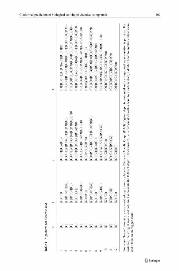
To apply machine learning techniques to this problem, the compounds must be describedin terms of a number of numerical attributes. There are several approaches to do this.The approach that was followed in this study is to compute signature descriptors2 [8].Each signature corresponds a specially constructed directed acyclic labelled subgraph inthe molecule graph. Signatures have a height, which corresponds to the number of edgesbetween root and terminal nodes of the directed acyclic subgraphs. In this exercise thesignatures had at most height 3. The signature descriptor for a molecule consists of the sig-natures present in the molecule along with their counts, i.e. the number of times the labelledsubgraph of a signature occur in the graph of the molecule. An example of the signaturedescriptor for ascorbic acid (also known as vitamin C) is provided in Fig. 1, Tables 1 and 2.

To create a data set from a number of compounds, all the signatures in all compounds arefirst enumerated and the set of all signatures is obtained. Each unique signature correspondsto one attribute, hence one dimension of the data set. To build the matrix of training exam-ples, each signature in the set is attributed (arbitrarily) a column index and each compounda row index. Each cell of the matrix contains the count of the occurrences of the signa-ture corresponding to the column in the compound corresponding to the row. The resultingmatrix can be very large but it is also highly sparse, as detailed further on (see Table 4).

3.1 Underlying algorithms

As a first step in the study, we set out to extract relevant non-conformity measures from dif-ferent underlying algorithms: Support Vector Machines (SVM), Nearest Neighbours, NaıveBayes. The Non Conformity Measures for each of the three underlying algorithms are listedin Table 3.

There are a number of considerations arising from the application of each of thesealgorithms to Compound Activity Prediction.

2The signature descriptors and other types of descriptors (e.g. circular descriptors) can be computed with theCDK (Chemistry Development Kit) Java package or any of its adaptations such as the RCDK package forthe R statistical software.

Conformal prediction of biological activity of chemical compounds 109

Tabl

e1

Sign

atur

esfo

ras

corb

icac

id

01

23

1[O

][O

]([C

])[O

]([C

]([C

]=[C

]))

[O](

[C](

[C](

[C][

O])

=[C

]([C

][O

])))

2[C

][C

]([C

]=[C

][O

])[C

]([C

]([C

][O

])=

[C](

[C][

O])

[O])

[C](

=[C

]([C

](=

[O][

O,0

])[O

])[C

]([C

]([C

][O

])[O

,0...

3[C

][C

]([C

][C

][O

])[C

]([C

]([C

][O

])[C

](=

[C][

O])

[O](

[C])

)[C

]([C

]([C

]([O

])[O

])[C

](=

[C](

[C,0

][O

])[O

])[O

](...

4[O

][O

]([C

][C

])[O

]([C

]([C

][C

])[C

]([C

]=[O

]))

[O](

[C](

[C](

=[C

,0][

O])

=[O

])[C

]([C

]([C

][O

])[C

,0...

5[C

][C

]([C

][O

]=[O

])[C

]([C

](=

[C][

O])

=[O

][O

]([C

]))

[C](

[C](

=[C

]([C

,0][

O])

[O])

=[O

][O

]([C

,0](

[C])

))

6[O

][O

](=

[C])

[O](

=[C

]([C

][O

]))

[O](

=[C

]([C

](=

[C][

O])

[O](

[C])

))

7[C

][C

]([C

]=[C

][O

])[C

](=

[C](

[C][

O])

[C](

[O]=

[O])

[O])

[C](

[C](

=[O

][O

]([C

,0])

)=[C

]([C

,0](

[C])

[O])

[O])

8[O

][O

]([C

])[O

]([C

]([C

]=[C

]))

[O](

[C](

=[C

]([C

][O

])[C

]([O

]=[O

])))

9[C

][C

]([C

][C

][O

])[C

]([C

]([O

])[C

]([C

][O

])[O

])[C

]([C

]([O

])[C

]([C

](=

[C][

O])

[O](

[C])

)[O

])

10[O

][O

]([C

])[O

]([C

]([C

][C

]))

[O](

[C](

[C](

[O])

[C](

[C][

O])

))

11[C

][C

]([C

][O

])[C

]([C

]([C

][O

])[O

])[C

]([C

]([C

]([C

][O

])[O

])[O

])

12[O

][O

]([C

])[O

]([C

]([C

]))

[O](

[C](

[C](

[C][

O])

))

For

ever

y“h

eavy

”at

om(i

.e.e

very

non-

hydr

ogen

atom

),a

labe

lled

Dir

ecte

dA

cycl

icG

raph

(DA

G)

ofgi

ven

dept

his

com

pute

dan

da

stri

ng-b

ased

repr

esen

tatio

nis

prov

ided

.For

inst

ance

,the

stri

ngat

row

7an

dco

lum

n1

repr

esen

tsth

eD

AG

ofde

pth

1fr

omat

om7,

i.e.a

carb

onat

omw

itha

bond

toa

carb

onat

om,a

doub

lebo

ndto

anot

her

carb

onat

oman

da

bond

toan

oxyg

enat

om

110 P. Toccaceli et al.

Table 2 Signature descriptor for ascorbic acid

Counts Signature

6 [C]

6 [O]

4 [O]([C])

2 [C]([C]=[C][O])

2 [C]([C][C][O])

2 [O]([C]([C]=[C]))

1 [C](=[C]([C](=[O][O,0])[O])[C]([C]([C][O])[O,0])[O])

1 [C](=[C]([C][O])[C]([O]=[O])[O])

1 [C]([C](=[C]([C,0][O])[O])=[O][O]([C,0]([C])))

1 [C]([C](=[C][O])=[O][O]([C]))

1 [C]([C](=[O][O]([C,0]))=[C]([C,0]([C])[O])[O])

1 [C]([C]([C]([C][O])[O])[O])

1 [C]([C]([C]([O])[O])[C](=[C]([C,0][O])[O])[O]([C,0](=[O])))

1 [C]([C]([C][O])=[C]([C][O])[O])

1 [C]([C]([C][O])[C](=[C][O])[O]([C]))

1 [C]([C]([C][O])[O])

1 [C]([C]([O])[C]([C](=[C][O])[O]([C]))[O])

1 [C]([C]([O])[C]([C][O])[O])

1 [C]([C][O])

1 [C]([C][O]=[O])

1 [O](=[C]([C](=[C][O])[O]([C])))

1 [O](=[C]([C][O]))

1 [O](=[C])

1 [O]([C](=[C]([C][O])[C]([O]=[O])))

1 [O]([C]([C](=[C,0][O])=[O])[C]([C]([C][O])[C,0]([O])))

1 [O]([C]([C]([C][O])))

1 [O]([C]([C]([C][O])=[C]([C][O])))

1 [O]([C]([C]([O])[C]([C][O])))

1 [O]([C]([C]))

1 [O]([C]([C][C]))

1 [O]([C]([C][C])[C]([C]=[O]))

1 [O]([C][C])

Each signature is used as a feature (a dimension); the number of occurrences is the value of the feature

SVM The usage of SVM in this domain poses a number of challenges. First of all, thenumber of training examples was large enough to create a problem for our computationalresources. The scaling of SVM to large data sets is indeed an active research area [2, 7, 18,19]. We turned our attention to a simple approach proposed by V.Vapnik et al. in [11], calledCascade SVM.

The sizes of the training sets considered here are too large to be handled comfortably bygenerally available SVM implementations, such as libsvm [6]. The approach we followcould be construed as a form of training set editing. Vapnik proved formally that it is possi-ble to decompose the training into an n-ary tree of SVM trainings. The first layer of SVMs

Conformal prediction of biological activity of chemical compounds 111

Table 3 The non conformity measures for the three underlying algorithms

Underlying Non conformity measure αi Comment

Support Vector Machine (SVM) −yid(xi ) (signed) distance between the example andthe separating hyperplane

k Nearest Neighbours (kNN)

∑(k)j �=i:yj =yi

d(xj ,xi )

∑(k)j �=i:yj �=yi

d(xj ,xi )Here the summation is on the k smallest val-ues of the distance between the example andits neighbours from same/other class

Naıve Bayes −log p(yi = c|xi) p is the posterior probability of the exam-ple’s class estimated by Naıve Bayes

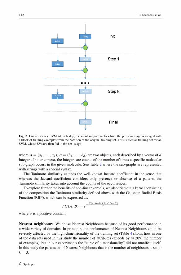
is trained on training sets obtained as a partition of the overall training set. Each SVM inthe first layer outputs its set of support vectors (SVs) which is generally smaller than thetraining set. In the second layer, each SVM takes as training set the merging of n of the SVssets found in the first layer. Each layer requires fewer SVMs. The process is repeated until alayer requires only one SVM. The set of SVs emerging from the last layer is not necessarilythe same that would be obtained by training on the whole set (but it is often a good approxi-mation). If one wants to obtain that set, the whole training tree should be executed again, butthis time the SVs obtained at the last layer would be merged into each of the initial trainingblocks. A new set of SVs would then be obtained at the end of the tree of SVMs. If this newset is the same as the one in the previous iteration, this is the desired set. If not, the processis repeated once more. In [11] it was proved that the process converges and that it convergesto the same set of SVs that one would obtain by training on the whole training set in one go.

To give an intuitive justification, the fundamental observation is that the SVM decisionfunction is entirely defined just by the Support Vectors. It is as if these examples containedall the information necessary for the classification. Moreover, if we had a training set com-posed only of the SVs, we would have obtained the same decision function. So, one mightas well remove the non-SVs altogether from the training set.

In experiments discussed here, we followed a simplified approach. Instead of a tree ofSVMs, we opted for a linear arrangement as shown in Fig. 2.

While we have no theoretical support for this semi-online variant of the Cascade SVM,the method appears to work satisfactorily in practice on the data sets we used.

The class imbalance was addressed with the use of per-class weighting of the C hyper-parameter, which results in a different penalization of the margin violations. The per-classweight was set inversely proportional to the class representation in the training set.

Another feature of SVM is the choice of an appropriate kernel. While we appreciatedthe computational advantages of linear SVM, we also believed that it was not necessarilythe best choice for the specific problem. It can easily be observed that the nature of therepresentation of the training objects (as discrete features) warranted approaches similar tothose used in Information Retrieval, where objects are described in terms of occurrencesof patterns (bags of words). The topic of similarity searching in chemistry is an active oneand there are many alternative proposals (see [1]). We used as a kernel a function calledTanimoto similarity3 defined as:

T (A,B) =∑d

i=1 min(ai, bi)∑d

i=1(ai + bi) − ∑di=1 min(ai, bi)

3See [10] for a proof that Tanimoto Similarity is a kernel.

112 P. Toccaceli et al.

Fig. 2 Linear cascade SVM At each step, the set of support vectors from the previous stage is merged witha block of training examples from the partition of the original training set. This is used as training set for anSVM, whose SVs are then fed to the next stage

where A = (a1, . . . , ad), B = (b1, . . . , bd) are two objects, each described by a vector of d

integers. In our context, the integers are counts of the number of times a specific molecularsub-graph occurs in the given molecule. See Table 2 where the sub-graphs are representedwith strings with a special syntax.

The Tanimoto similarity extends the well-known Jaccard coefficient in the sense thatwhereas the Jaccard coefficient considers only presence or absence of a pattern, theTanimoto similarity takes into account the counts of the occurrences.

To explore further the benefits of non-linear kernels, we also tried out a kernel consistingof the composition the Tanimoto similarity defined above with the Gaussian Radial BasisFunction (RBF), which can be expressed as.

T G(A,B) = e− |T (A,A)+T (B,B)−2T (A,B)|

γ

where γ is a positive constant.

Nearest neighbours We chose Nearest Neighbours because of its good performance ina wide variety of domains. In principle, the performance of Nearest Neighbours could beseverely affected by the high-dimensionality of the training set (Table 4 shows how in oneof the data sets used in this study the number of attributes exceeds by ≈ 20% the numberof examples), but in our experiments the “curse of dimensionality” did not manifest itself.In this study the parameter of Nearest Neighbours that is the number of neighbours is set tok = 3.

Conformal prediction of biological activity of chemical compounds 113

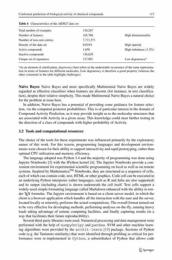
Table 4 Characteristics of the AID827 data set

Total number of examples 138,287

Number of features 165,786 High dimensionality

Number of non-zero entries 7,711,571

Density of the data set 0.034% High sparsity

Active compounds 1,658 High imbalance (1.2%)

Inactive compounds 136,629

Unique set of signatures 137,901 Low degeneracya

aAs an element of clarification, degeneracy here refers to the undesirable occurrence of the same representa-tion in terms of features for different molecules. Low degeneracy is therefore a good property (whereas theother comments in the table highlight challenges)

Naıve Bayes Naıve Bayes and more specifically Multinomial Naıve Bayes are widelyregarded as effective classifiers when features are discrete (for instance, in text classifica-tion), despite their relative simplicity. This made Multinomial Naıve Bayes a natural choicefor the problem at issue here.

In addition, Naıve Bayes has a potential of providing some guidance for feature selec-tion, via the computed posterior probabilities. This is of particular interest in the domain ofCompound Activity Prediction, as it may provide insight as to the molecular structures thatare associated with Activity in a given assay. This knowledge could steer further testing inthe direction of a class of compounds with higher probability of Activity.

3.2 Tools and computational resources

The choice of the tools for these experiments was influenced primarily by the exploratorynature of this work. For this reason, programming languages and development environ-ments were chosen for their ability to support interactivity and rapid prototyping, rather thanoptimal CPU utilization and memory efficiency.

The language adopted was Python 3.4 and the majority of programming was done usingJupyter Notebooks [5] with the IPython kernel [4]. The Jupyter Notebooks provide a con-venient environment for experimental scientific programming on local as well as on remotesystems. Inspired by MathematicaTM Notebooks, they are structured as a sequence of cells,each of which can contain code, text, HTML or other graphics. Code cell can be executed inan underlying Python interpreter (other languages, such as R and Julia are also supported)and its output (including charts) is shown underneath the cell itself. Text cells support awidely-used simple formatting language called Markdown enhanced with the ability to ren-der TEX formulas. The Jupyter environment is based on a client-server model, in which theclient is a browser application which handles all the interaction with the user and the server,located locally or remotely, performs the actual computations. The overall format turned outto be very effective for developing methods, performing analyses on-the-fly, running heavyloads taking advantage of remote computing facilities, and finally capturing results (in away that facilitates their future reproducibility).

Several third-party libraries were used. Numerical processing and data management wereperformed with the help of numpy/scipy and pandas. SVM and other machine learn-ing algorithms were provided by the scikit-learn [13] package. Sections of Pythoncode (e.g. the Tanimoto similarity) that were identified through profiling as critical for per-formance were re-implemented in Cython, a subset/dialect of Python that allows code

114 P. Toccaceli et al.

to be compiled (via an intermediate C representation) rather than being interpreted. Thecomputations were run initially on a local server (8 cores with 32GB of RAM, runningOpenSuSE) and in later stages on a supercomputer, the IT4I Salomon cluster located inOstrava, Czech Republic. The Salomon cluster is based on the SGI ICE X system and com-prises 1008 computational nodes (plus a number of login nodes), each with 24 cores (212-core Intel Xeon E5-2680v3 2.5GHz processors) and 128GB RAM, connected via high-speed 7D Enhanced hypercube InfiniBand FDR and Ethernet networks. It currently ranksat #48 in the top500.org list of supercomputers and at #14 in Europe.4

Parallelization and computation distribution relied on the ipyparallel [3] package,which is a high-level framework for the coordination of remote execution of Python func-tions on a generic collection of nodes (cores or separate servers). While ipyparallelmay not be highly optimized, it aims at providing a convenient environment for distributedcomputing well integrated with IPython and Jupyter and has a learning curve that is notas steep as that of the alternative frameworks common in High Performance Computing(OpenMPI, for example). In particular, ipyparallel, in addition to allowing the start-up and shut-down of a cluster comprising a controller and a number of engines where theactual processing (each is a separate process running a Python interpreter) is performed viaintegration with the job scheduling infrastructure present on Salomon (PBS, Portable BatchSystem), took care of the details such as data serialization/deserialization and transfer, loadbalancing, job tracking, exception propagation, etc. thereby hiding much of the complexityof parallelization. One key characteristic of ipyparallel is that, while it provides prim-itives for map() and reduce(), it does not constrain the choice to those two, leaving theimplementer free to select the most appropriate parallel programming design patterns forthe specific problem (see [23] for a reference on the subject).

In this work, parallelization was exploited to speed up the computation of the Grammatrix or of the decision function for the SVMs or the matrix of distances for kNN. In eithercase, the overall task was partitioned in smaller chunks that were then assigned to engines(each running on a core on a node), which would then asynchronously return the result.Also, parallelization was used for SVM cross-validation, but at a coarser granularity, i.e.one engine per SVM training with a parameter. Data transfers were minimized by makinguse of shared memory where possible and appropriate. A key speed-up was achieved byusing pre-computed kernels (computed once only) when performing Cross-Validation withrespect to the hyperparameter C.

A zip archive with the code and the data files used to obtain the results presented inthis paper is available at http://clrc.rhul.ac.uk/people/ptocca/AMAI-2017/20170113-AMAI-Package.zip.

3.3 Results

To assess the relative merits of the different underlying algorithms, we applied InductiveMondrian Conformal Predictors on data set AID827, whose characteristics are listed inTable 4.

The test was articulated in 20 cycles of training and evaluation. In each cycle, a test setof 10,000 examples was extracted at random. The remaining examples were split randomlyinto a proper training set of 100,000 examples and a calibration set with the balance of theexamples (28,387).

4According to https://www.sgi.com/company info/newsroom/press releases/2015/september/salomon.html.

Conformal prediction of biological activity of chemical compounds 115

During the SVM training, 5-fold stratified cross validation was performed at every stageof the Cascade to select an optimal value for the hyperparameter C. Also, per-class weightswere assigned to cater for the high class imbalance in the data, so that a higher penalizationwas applied to violators in the less represented class.

In Multinomial Naıve Bayes too, cross validation was used to choose an optimal valuefor the smoothing parameter.

The results are listed in Table 5, which presents the classification arising from the regionpredictor for ε = 0.01. The numbers are averages over the 20 cycles of training and testing.

Note that a compound is classified as Active (resp. Inactive) if and only if Active (resp.Inactive) is the only label in the prediction set. When both labels are in the prediction, theprediction is considered Uncertain.

It has to be noted at this stage that there does not seem to be an established consensuson what the best performance criteria are in the domain of Compound Activity Prediction(see for instance [12]), although Precision (fraction of actual Actives among compoundspredicted as Active) and Recall (fraction of all the Active compounds that are among thosepredicted as Active) seem to be generally relevant. In addition, it is worth pointing out thatthese (and many other) criteria of performance should be considered as generalisations ofclassical performance criteria since they include dependence of the results on the requiredconfidence level.

At the shown significance level of ε = 0.01, 34% of the compounds predicted as Activeby Inductive Mondrian Conformal Prediction using Tanimoto composed with Gaussian RBFwere actually Active compared to a prevalence of Actives in the data set of just 1.2%. Atthe same time, the Recall was ≈ 41% (ratio of Actives in the prediction to total Actives inthe test set).

We selected Cascade SVM with Tanimoto+RBF as the most promising underlying algo-rithm on the basis of the combination of its high Recall (for Actives) and high Precision(for Actives), assuming that the intended application is indeed to output a selection ofcompounds that has a high prevalence of Active compounds.

Note that in Table 5 the values similar to ones of confusion matrix are calculated onlyfor certain predictions. In this representation, the concrete meaning of the property of class-based validity can be clearly illustrated as in Table 6: the two rightmost columns report the

Table 5 Conformal predictors results for AID827 with significance ε = 0.01

Underlying Active pred Inactive pred Inactive pred Active pred Empty Uncertain

Active Active Inactive Inactive pred

Naıve Bayes 38.20 104.30 183.30 1.10 0 9673.10

3NN 43.95 100.55 361.55 0.80 0 9493.15

Cascade SVM:

– linear 34.20 99.00 591.85 1.20 0 9273.75

– RBF kernel 47.20 101.80 1126.75 1.80 0 8722.45

– Tanimoto kernel 48.45 97.65 986.85 0.80 0 8866.25

– Tanimoto-RBF kernel 47.65 94.10 1044.90 0.95 0 8812.40

All results are averages over 20 runs, using the same test sets of 10,000 objects across the different under-lying algorithms. “Active predicted Active” is the (average) count of actually Active test examples that werepredicted Active by Conformal Prediction. Uncertain predictions occur when both labels are output by theregion predictor. Empty predictions occur when both labels can be rejected at the chosen significance level.For the specific significance level chosen here, there were never empty predictions

116 P. Toccaceli et al.

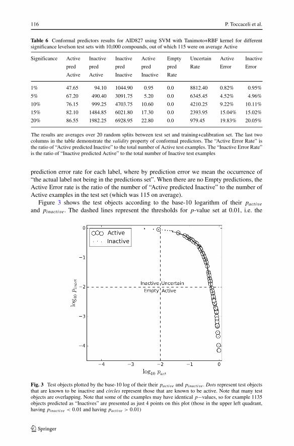
Table 6 Conformal predictors results for AID827 using SVM with Tanimoto+RBF kernel for differentsignificance levelson test sets with 10,000 compounds, out of which 115 were on average Active

Significance Active Inactive Inactive Active Empty Uncertain Active Inactive

pred pred pred pred pred Rate Error Error

Active Active Inactive Inactive Rate

1% 47.65 94.10 1044.90 0.95 0.0 8812.40 0.82% 0.95%

5% 67.20 490.40 3091.75 5.20 0.0 6345.45 4.52% 4.96%

10% 76.15 999.25 4703.75 10.60 0.0 4210.25 9.22% 10.11%

15% 82.10 1484.85 6021.80 17.30 0.0 2393.95 15.04% 15.02%

20% 86.55 1982.25 6928.95 22.80 0.0 979.45 19.83% 20.05%

The results are averages over 20 random splits between test set and training+calibration set. The last twocolumns in the table demonstrate the validity property of conformal predictors. The “Active Error Rate” isthe ratio of “Active predicted Inactive” to the total number of Active test examples. The “Inactive Error Rate”is the ratio of “Inactive predicted Active” to the total number of Inactive test examples

prediction error rate for each label, where by prediction error we mean the occurrence of“the actual label not being in the predictions set”. When there are no Empty predictions, theActive Error rate is the ratio of the number of “Active predicted Inactive” to the number ofActive examples in the test set (which was 115 on average).

Figure 3 shows the test objects according to the base-10 logarithm of their pactive

and pinactive. The dashed lines represent the thresholds for p-value set at 0.01, i.e. the

Fig. 3 Test objects plotted by the base-10 log of their their pactive and pinactive . Dots represent test objectsthat are known to be inactive and circles represent those that are known to be active. Note that many testobjects are overlapping. Note that some of the examples may have identical p−values, so for example 1135objects predicted as “Inactives” are presented as just 4 points on this plot (those in the upper left quadrant,having pinactive < 0.01 and having pactive > 0.01)

Conformal prediction of biological activity of chemical compounds 117

significance value ε used in Table 5. The two dashed lines partition the plane in 4 regions,corresponding to the region prediction being Active (pactive > ε and pinactive ≤ ε), Inac-tive (pactive ≤ ε and pinactive > ε), Empty (pactive ≤ ε and pinactive ≤ ε), Uncertain(pactive > ε and pinactive > ε).

As we indicated in Section 2.1, the alternative is forced prediction with individualconfidence and credibility.

It is clear that there are several benefits accruing from using Conformal Predictors.For instance, a high p-value for the Active hypothesis might suggest that Activity can-not be ruled out, but the same compound may exhibit also a high p-value for the Inactivehypothesis, which would actually mean that neither hypothesis could be discounted.

In this specific context it can be argued that the p-values for Active hypothesis are moreimportant. They can be used to rank the test compounds like it was done in [21] for rankingpotential interaction. A high p-value for the Active hypothesis might suggest that Activitycannot be ruled out. For example it is possible to output the prediction list of all compoundswith p-values above a threshold ε = 0.01. A concrete activity which is not yet discoveredwill be covered by this list with probability 0.99. All the remaining examples are classifiedas Non-Active with confidence 0.99 or larger.

Special attention should be also paid to low credibility examples where both p-valuesare small. Such examples might appear in the “Empty” quarter of the plot on Fig. 3 if thethreshold were changed. For such examples, the label assignment does not conform to thetraining data. They may be considered as anomalies or examples of compound types notenough represented in the training set. This may suggest that it would be beneficial to theoverall performance of the classifier to perform a lab test for those compounds and includethe results in training set.

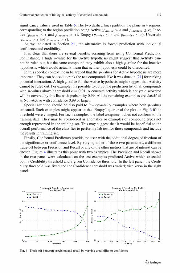
Finally, Conformal Predictors provide the user with the additional degree of freedom ofthe significance or confidence level. By varying either of those two parameters, a differenttrade-off between Precision and Recall or any of the other metrics that are of interest can bechosen. Figure 4 illustrates this point with two examples. The Precision and Recall shownin the two panes were calculated on the test examples predicted Active which exceededboth a Credibility threshold and a given Confidence threshold. In the left panel, the Credi-bility threshold was fixed and the Confidence threshold was varied; vice versa in the rightpanel.

Fig. 4 Trade-off between precision and recall by varying credibility or confidence

118 P. Toccaceli et al.

3.4 Application to different data sets

We applied Inductive Conformal Predictors with underlying SVM using Tanimoto+RBFkernel to other data sets extracted from PubChem BioAssay to verify if the same perfor-mance would be achieved for assays covering a range of quite different biological targetsand to what extent the performance would vary with differences in training set size, imbal-ance, and sparseness of the training set. The main characteristics of the data sets are reportedin Table 7.

As in the previous set of experiments, 20 cycles of training and testing were performedand the results averaged over them. In each cycle, a test set of 10,000 examples was setaside and the rest was split between calibration set (≈ 30, 000) and proper training set. Theresults are reported in Table 8.

It can be seen that the five data sets differ in their hardness for machine learning andin particular some of them produce more uncertain predictions using the same algorithms,number of examples and the same significance level.

3.5 Mondrian ICP with different εactive and εinactive

When applying Mondrian ICP, there is no constraint to use the same significance ε for thetwo labels. Using two different significance levels allows to vary the relative importance of

Table 7 Data sets and their characteristics

Data set Assay description Number of Number of Actives (%) Density (%)

compounds features

827 High Throughput Screen to Identify 138,287 165,786 1.2% 0.034%

Compounds that Suppress the

Growth of Cells with a Deletion

of the PTEN Tumor Suppressor

1461 qHTS Assay for Antagonists of the 208,069 211,474 1.11% 0.026%

Neuropeptide S Receptor: cAMP

Signal Transduction

1974 Fluorescence polarization-based 302,310 237,837 1.05% 0.024%

counterscreen for RBBP9 inhibitors:

primary biochemical high throughput

screening assay to identify inhibitors

of the oxidoreductase glutathione

S-transferase omega 1(GSTO1)

2553 High throughput screening of inhibitors 305,308 236,508 1.06% 0.024%

of transient receptor potential cation

channel C6 (TRPC6)

2716 Luminescence Microorganism 298,996 237,811 1.02% 0.024%

Primary HTS to Identify Inhibitors

of the SUMOylation Pathway

Using a Temperature Sensitive

Growth Reversal Mutant Mot1-301

Density refers to the percentage of non-zero entries in the full matrix of ‘Number of Compounds × Numberof Features’ elements

Conformal prediction of biological activity of chemical compounds 119

Table 8 Results of the application of Mondrian ICP with ε = 0.01 using SVM with Tanimoto+RBF asunderlying

DataSet Active pred Inactive pred Inactive pred Active pred Empty Uncertain

Active Active Inactive Inactive pred

827 47.65 94.10 1044.90 0.95 0 8812.40

1461 29.45 101.30 1891.10 1.20 0 7976.95

1974 62.50 97.40 880.85 1.00 0 8958.25

2553 34.00 101.00 337.90 1.00 0 9526.10

2716 3.55 98.20 97.00 1.00 0 9800.25

Test set size: 10,000

the two kinds of mis-classifications. Indeed, there may be an advantage in allowing different“error” rates for the two labels especially when the focus might be on identifying Activesrather than Inactives.

The validity of Mondrian machines implies that the expected number of certain butwrong predictions is bounded by εact for (true) actives and by εinact for (true) non-actives.

Figure 5 shows the trade-off between Precision and Recall that results from varyingεinact .

For very low values of the significance ε, a large number of test examples have pact >

εact as well as pinact > εinact . For these test examples, we have an ‘Uncertain’ prediction.As we increase εinact , fewer examples have a pinact larger than εinact . So ‘Inactive’ is

not chosen any longer as a label for those examples. If they happen to have a pact > εact ,

Fig. 5 Trade-off between precision and recall by varying εinact

120 P. Toccaceli et al.

they switch from ‘Uncertain’ to being predicted as ‘Active’ (in the other case, they wouldbecome ‘Empty’ predictions).

Figure 6 shows how Precision varies with Recall using three methods: varying the thresh-old applied to the Decision Function of the underlying SVM, varying the significance εinact

for the Inactive class, varying the credibility. The three methods appear to give similarresults and might seem equivalent. In the next section, we discuss a perspective that is ofpractical interest and that is quite specific to the CP technique.

4 Ranking of compounds by p-value

A useful product of the application of Conformal Predictors is the ability to rank the com-pounds by the p-values. A similar approach was applied to protein-protein interactions in[21].

In this specific context, where the focus is primarily on identifying the compounds thatare more likely to be active towards a given biological target, the desired ranking wouldnaturally list the candidates by pactive in descending order (i.e. compounds with higher p-value would rank higher than compounds with lower p-value) and break any ties using thepinactive (in ascending order).

An example of the ranking that can be obtained in this way is illustrated in Table 9. Thetable lists the 20 compounds that were assigned the largest pactive values in one of the runs.As explained earlier, these are the compounds for which there was the largest proportion ofcalibration compounds for which the Non Conformity Measure was greater than or equalto the Non Conformity Measure associated to the hypothesis of the compound being active.This last sentence is not clear - we probably don’t need this sentence at all. We also need tosay a bit more about good predictions we have made here.

Fig. 6 Precision vs. recall: three methods

Conformal prediction of biological activity of chemical compounds 121

Table 9 The 20 candidatecompounds (out of a held-out testset of 10,000) with the largestpactive values, from one of theruns for the data set AID827

Ranking Compound ID pactive pinactive

1 108198 0.997067 0.000036

2 103948 0.988270 0.000072

3 62772 0.988270 0.000143

4 129143 0.982405 0.000143

5 108632 0.961877 0.000179

6 138051 0.961877 0.000179

7 108920 0.941349 0.000322

8 108877 0.938416 0.000322

9 108783 0.932551 0.000322

10 107957 0.932551 0.000322

11 5413 0.926686 0.000358

12 4334 0.923754 0.000394

13 138177 0.923754 0.000394

14 71538 0.914956 0.000537

15 54806 0.914956 0.000537

16 16925 0.903226 0.000608

17 108026 0.903226 0.000644

18 108584 0.900293 0.000644

19 107943 0.894428 0.000644

20 108032 0.894428 0.000644

Bold face denotes thosecompounds that are actuallyActive. The compound ID is justthe index in the pre-processeddata set and not the PubChem ID

We believe this product of the application of CP is of particular practical interest becauseit allows the user (e.g. a pharmaceutical company) to select a set of promising compoundswith a chosen level confidence.

5 Conclusions

This paper summarized a methodology of applying Mondrian Conformal Predictors to bigand imbalanced data with several underlying machine learning methods like nearest neigh-bours, Bayesian, SVM and various kernels. The results have been compared from the pointof view of efficiency of various methods and various sizes of the data sets. The paper alsodemonstrated how the error rate can be effectively controlled by changing the confidencelevel for the prediction. Lastly and perhaps most importantly, the paper provided an exam-ple of how Conformal Predictors can be used to rank compounds based on the confidence intheir activity. Such ranking can be extremely useful in guiding the choice of the compoundsto test, with the potential of reducing dramatically the investments required for identifyingnew candidate drugs.

The most interesting direction of the future extension is to study the possible strategiesof active learning (or experimental design) and the practical problem of their integrationinto an on-going drug development process. The methods employed in this paper produce anumber of uncertain predictions, in which both the Active and Inactive hypotheses cannot berejected. It might be useful to select among those uncertain cases the compounds that shouldbe checked experimentally first – in other words the most “promising” compounds. How

122 P. Toccaceli et al.

to select though may depend on practical scenarios of further learning and on comparativeefficiency of different active learning strategies.

Acknowledgments This project (ExCAPE) has received funding from the European Union’s Horizon 2020Research and Innovation programme under Grant Agreement no. 671555. We are grateful for the help in con-ducting experiments to the Ministry of Education, Youth and Sports (Czech Republic) that supports the LargeInfrastructures for Research, Experimental Development and Innovations project “IT4Innovations NationalSupercomputing Center – LM2015070”. This work was also supported by EPSRC grant EP/K033344/1(“Mining the Network Behaviour of Bots”) and by Technology Integrated Health Management (TIHM)project awarded to the School of Mathematics and Information Security at Royal Holloway as part of an ini-tiative by NHS England supported by InnovateUK. We are indebted to Lars Carlsson of Astra Zeneca forproviding the data and useful discussions. We are also thankful to Zhiyuan Luo and Vladimir Vovk for manyvaluable comments and discussions.

Open Access This article is distributed under the terms of the Creative Commons Attribution 4.0 Inter-national License (http://creativecommons.org/licenses/by/4.0/), which permits unrestricted use, distribution,and reproduction in any medium, provided you give appropriate credit to the original author(s) and the source,provide a link to the Creative Commons license, and indicate if changes were made.

References

1. Monev, V.: Introduction to similarity searching in chemistry. Comm. Math. Comp. Chem. 51, 7–38(2004)

2. Bottou, L., Chapelle, O., DeCoste, D., Weston, J.: Large-scale kernel machines (neural informationprocessing). The MIT press (2007)

3. Bussonnier, M.: Interactive parallel computing in Python. https://github.com/ipython/ipyparallel4. Perez, F., Granger, B.E.: IPython: a system for interactive scientific computing, vol. 9 (2007). http://

ipython.org5. Kluyver, T., et al.: Jupyter Notebooks – a publishing format for reproducible computational

workflows. Positioning and Power in Academic Publishing: Players, Agents and Agendas, 87–90doi:10.3233/978-1-61499-649-1-87

6. Chang, C.-C., Lin, C.-J.: LIBSVM: A library for support vector machines. ACM Trans. Intell. Syst.Technol. 2, 27:1–27:27 (2011). Software available at http://www.csie.ntu.edu.tw/∼cjlin/libsvm

7. Chang, E.Y.: PSVM: parallelizing support vector machines on distributed computers. In: Foundationsof Large-Scale Multimedia Information Management and Retrieval, pp. 213–230. Springer, BerlinHeidelberg (2011)

8. Faulon, J.-L., Visco, D.P. Jr., Pophale, R.S.: The signature molecular descriptor. 1. using extendedvalence sequences in qsar and qspr studies. J. Chem. Inf. Comput. Sci. 43(3), 707–720 (2003). PMID:12767129

9. Gammerman, A., Vovk, V.: Hedging predictions in machine learning. Comput. J. 50(2), 151–163 (2007)10. Gartner, T.: Kernels for Structured Data. World Scientific Publishing Co., Inc., River Edge (2009)11. Graf, H.P., Cosatto, E., Bottou, L., Durdanovic, I., Vapnik, V.: Parallel support vector machines: the

cascade SVM. In: Advances in Neural Information Processing Systems, pp. 521–528. MIT Press (2005)12. Jain, A.N., Nicholls, A.: Recommendations for evaluation of computational methods. J. Comput. Aided

Mol. Des. 22(3-4), 133–139 (2008)13. Pedregosa, F., Varoquaux, G., Gramfort, A., Michel, V., Thirion, B., Grisel, O., Blondel, M., Pretten-

hofer, P., Weiss, R., Dubourg, V., Vanderplas, J., Passos, A., Cournapeau, D., Brucher, M., Perrot, M.,Duchesnay, E.: Scikit-learn: Machine learning in Python. J. Mach. Learn. Res. 12, 2825–2830 (2011)

14. Shafer, G., Vovk, V.: A tutorial on conformal prediction. J. Mach. Learn Res. 9, 371–421 (2008)15. Vovk, V., Gammerman, A., Shafer, G.: Algorithmic Learning in a Random World. Springer-Verlag New

York, Inc., Secaucus, NJ, USA (2005)16. Weis, D.C., Visco, D.P. Jr.: Jean-loup Faulon. Data mining pubchem using a support vector machine

with the signature molecular descriptor Classification of factor {XIa} inhibitors. J. Mol. Graph. Model.27(4), 466 –475 (2008)

17. Holenz, J., et al. (eds.): Lead Generation: Methods and Strategies, vol. 68. Wiley-VCH (2016)18. Woodsend, K., Gondziom, J.: Hybrid MPI/OpenMP parallel linear support vector machine training. J.

Mach. Learn. Res. 10, 1937–1953 (2009)

Conformal prediction of biological activity of chemical compounds 123

19. You, Y., Fu, H., Song, S.L., Randles, A., Kerbyson, D., Marquez, A., Yang, G., Hoisie, A.: Scalingsupport vector machines on modern HPC platforms. J. Parallel Distrib. Comput. 76(C), 16–31 (2015)

20. Toccaceli, P., Nouretdinov, I., Gammerman, A.: Conformal predictors for compound activity prediction.In: COPA Proceedings of the 5th International Symposium on Conformal and Probabilistic Predictionwith Applications, vol. 9653, p. 2016. Springer-Verlag New York Inc. (2016)

21. Nouretdinov, I., Gammerman, A., Qi, Y., Klein-Seetharaman, J.: Determining confidence of predictedinteractions between HIV-1 and human proteins using conformal method. Pac. Symp. Biocomput. 311(2012)

22. Wang, Y., Suzek, T., Zhang, J., Wang, J., He, S., Cheng, T., Shoemaker, B.A., Gindulyte, A., Bryant,S.H.: Pubchem BioAssay: 2014 upyear. Nucleic Acids Res. 42(1), D1075–82 (2014)

23. McCool, M., Robison, A.D., Reinders, J.: Structured Parallel Programming: Patterns for EfficientComputation. Morgan-Kaufmann (2012)