confirming a plant‐mediated …¬rming a plant-mediated “biological tide” in an aridland...

Confirming a plant-mediated “Biological Tide” in anaridland constructed treatment wetland

PAUL BOIS,1,2 DANIEL L. CHILDERS,3,� THOMAS CORLOUER,2 JULIEN LAURENT,1,2

ANTOINE MASSICOT,2 CHRISTOPHER A. SANCHEZ,3 AND ADRIEN WANKO1,2

1ICube (UMR 7357 ENGEES/CNRS/Unistra), 2 rue Boussingault, 67000 Strasbourg, France2LTSER France, Zone Atelier Environnementale Urbaine, 3 Rue de l’Argonne, 67000 Strasbourg, France

3School of Sustainability, Arizona State University, Tempe, Arizona 85287 USA

Citation: Bois, P., D. L. Childers, T. Corlouer, J. Laurent, A. Massicot, C. A. Sanchez, and A. Wanko. 2017. Confirming aplant-mediated “Biological Tide” in an aridland constructed treatment wetland. Ecosphere 8(3):e01756. 10.1002/ecs2.1756

Abstract. As urban populations grow and the need for sustainable water treatment increases, urbanconstructed treatment wetlands (CTWs) are increasingly being used and studied. However, less is knownabout the effectiveness of this “turquoise infrastructure” in arid climates. In a recent publication, wepresented evidence of plant-mediated control of surface hydrology, using a water budget approach, in aCTW in Phoenix, Arizona, USA. We also demonstrated how this transpiration-driven wetland surface flowmade this treatment marsh more effective at pollutant removal than its counterparts in cooler or moremesic environments. Water budget-based calculations estimated that nearly 20% of the water overlying themarsh was transpired daily by the plants (40–60 L�m�2�d�1) during the hottest summer months. Weestimated the associated water velocity to be about 40 cm/h. In this paper, we report on hydrodynamicexperiments that confirmed the existence of this phenomenon that we refer to as the “Biological Tide,”and verified the rate at which transpiration by the marsh vegetation moves surface water into thebiogeochemically active marsh. We combined a water budget-based approach and dye tracer experimentsto quantify and confirm this phenomenon. Because of the low velocities estimated from our water budgetapproach (a few cm/h), we used a fixed-wall flowthrough marsh flume to limit the lateral dye movementduring the tracer experiments. We measured actual flow rates of 7–50 cm/h (with 5–8% precision) duringthese experiments, which closely conformed to the values estimated from our water budget-basedapproaches. The flow was largely dispersive due to the extensive impedance imparted by dense plantstems in the marsh. From these summer flow rates, we calculated that residence time of the wateroverlying the marsh in this CTW averaged about 13 d, but could be as low as four days. Again, thesevalues were reasonably close to the 15–20% replacement rate for marsh water we estimated using the waterbudget approach. This is the first time, to our knowledge, that plant-mediated biological control of surfacehydrology in a wetland, without connection to groundwater, has been reported.

Key words: constructed treatment wetland; dye tracer experiment; ecological engineering; transpiration; urbansustainability; wastewater treatment.

Received 14 December 2016; revised 13 February 2017; accepted 13 February 2017. Corresponding Editor: RyanA. Sponseller.Copyright: © 2017 Bois et al. This is an open access article under the terms of the Creative Commons AttributionLicense, which permits use, distribution and reproduction in any medium, provided the original work is properly cited.� E-mail: [email protected]

❖ www.esajournals.org 1 March 2017 ❖ Volume 8(3) ❖ Article e01756

info:doi/10.1002/ecs2.1756

info:doi/10.1002/ecs2.1756

http://creativecommons.org/licenses/by/3.0/

INTRODUCTION

Humans are becoming an increasingly urbanspecies: Since 1900 the proportion of people livingin cities has increased from 10% to over 50% glob-ally, and will likely be 80% by 2050 (Grimm et al.2008). In the last 100 yr, many cities have trans-formed into “sanitary cities,” with highly central-ized, capitalized, and expensive infrastructuredesigned to keep inhabitants healthy (Melosi2000, Grove 2009). Often this infrastructure hasimparted large systemic inertias on cities that hin-der novel or transformative new solutions togrowing problems (Childers et al. 2014). Still,there are many ways to design urban infrastruc-ture so as to optimize key ecosystem services byusing “design with nature” approaches that makecities more resilient and sustainable (Pickett et al.2013). When these urban designs incorporate ter-restrial ecological features, they are typicallycalled “green infrastructure,” while “blue infras-tructure” refers to aquatic systems. One exampleof “designing with nature” is the increasing use ofconstructed treatment wetlands (CTWs) as part ofurban wastewater treatment in place of expensiveand energy-intensive treatment technologies. Wet-lands have both terrestrial and aquatic ecologicalcharacteristics, and because of the color thatresults when green and blue are mixed, we referto such urban wetlands as “turquoise infrastruc-ture” (Childers et al. 2015).

Constructed treatment wetlands are a rela-tively low cost and low maintenance solution tourban wastewater and water reclamation chal-lenges (Wallace and Knight 2006, Nivala et al.2013). Most CTWs are designed to “polish” par-tially treated municipal effluent with a mix ofopen water areas, macrophytic vegetation, andwaterlogged soils (Fonder and Headley 2013).Designs are often highly dependent on local orregional variables, including water quality regu-lations and site-specific conditions (Fonder andHeadley 2010, Tanner et al. 2012), and rely ondifferent flow types (subsurface [SSF] vs. freewater surface [FWS] flow). While CTWs may berelatively similar in design and expectations, par-ticular attention must be paid to the way thesesystems function in different climatic settings.

Arid environments make up more than 30% ofthe earth’s land surface, and cities in these regionsincreasingly face water scarcity issues. To address

these issues, many are turning to the reuse of trea-ted municipal effluent for various urban uses(Greenway 2005), but the challenge is thatreclaimed water used in densely populated areasmust be clean. Notably, in the aridland city ofPhoenix, Arizona, USA—where we conducted theresearch reported here—virtually all municipaleffluent is reused (Metson et al. 2012), and theonly real export of water from the city is to theatmosphere. Constructed treatment wetlands area viable “design with nature” solution, but build-ing these wetlands in hot, arid cities such as Phoe-nix may expose them to unique challengesassociated with large losses of water via evapora-tion and plant transpiration. With this in mind,since summer 2011 we have been quantifyingthese water fluxes in a CTW operated by the Cityof Phoenix Water Services Department while alsomeasuring wetland plant biomass and estimatingthe whole-system water and nutrient budgets(Sanchez et al. 2016, Weller et al. 2016). Our objec-tive has been to understand the effect of atmo-spheric water losses on the whole-system waterbudget and on the ability of this CTW to removenitrogen from wastewater effluent. We foundlarge losses of water from the emergent marshesvia plant transpiration during the hot, dry sum-mer months—as much as 20–25% of the wateroverlying the vegetated marsh daily—and weidentified a horizontal advection of surface waterfrom nearby open water areas as the only way toreplace this transpired water. We call this phe-nomenon a “biological tide” (hereafter BiologicalTide; Sanchez et al. 2016), which is a different phe-nomenon from evapotranspiration-driven move-ments of shallow groundwater (White 1932, Baueret al. 2004, McLaughlin and Cohen 2014). Transpi-ration-driven movement of shallow SSF water hasbeen documented in a number of wetlands,including with tree islands in the Okavango Deltain Botswana (Bauer-Gottwein et al. 2007, Rambergand Wolski 2008) and in the Florida Everglades(Bazante et al. 2006, Troxler-Gann and Childers2006, Sullivan et al. 2014). However, to our knowl-edge, this is the first time that biotic control of sur-face hydrology has been demonstrated in anywetland. In this paper, we present data from twodifferent approaches that independently corrobo-rated this plant-driven movement of water into aCTW marsh, verifying that this unique, never-before-described phenomenon exists.


BOIS ET AL.

Furthermore, this plant-mediated BiologicalTide is actually increasing the nutrient removalefficacy of the CTW we studied: The vegetatedmarsh consistently removed virtually all of theinorganic nitrogen (N) made available to it,despite high rates of transpirational water loss(Sanchez et al. 2016). By bringing additional waterand solutes into the vegetated marsh and its soils,from adjacent open water areas, the BiologicalTide actually enhanced the ability of the marsh toremove N relative to CTWs found in cooler ormore mesic settings (Sanchez et al. 2016).

The objective of this work was to measureactual surface water flow within the marsh and tocompare these flow rates to those estimated usingour transpiration-based water budget calcula-tions. Often water flow measurement experimentsconducted in wetlands include the entire systemor flow rates on the order of cm/s (Leonard andLuther 1995, Leonard and Croft 2006). In this case,though, the spatial scale of our experiment wassmall and the magnitude of expected velocitieswas very low—a few cm/h. These challengesrequired a different methodological approach.One of the easiest ways to measure water veloci-ties is with a flowmeter, but this technique willnot work at low flow velocities (~0.4 cm/s)because of inappropriate detection limits. Dopplervelocimetry is an alternative, but Dopplerflowmeters typically require a minimum waterdepth on the order of 0.25–0.5 m (Meselhe et al.2004), and the water overlying vegetated wet-lands is often shallower than this. Plant stems alsointerfere with the propagation of the acoustic sig-nal, making Doppler results from vegetated wet-lands difficult to obtain or analyze. In our CTWstudy site, water depths in the vegetated marshaveraged roughly 0.25 m, plant densities and pro-ductivity were high (Weller et al. 2016), and byour estimates, the Biological Tide flowed at only afew cm/h. Therefore, the only viable technique fordocumenting this flow was a tracer experiment.

The application of tracer studies to wetlands isnot new (Bowmer 1987). Such tracer experimentshave been used to calibrate hydrodynamic mod-els of secondary and tertiary treatment wetlands(Giraldi et al. 2009, Laurent et al. 2015), to studyon the effects of vegetation on flow dynamics(Bodin et al. 2012), to study internal wetlandflows (Williams and Nelson 2011), and to examinethe influence of water flow on CTW capacity

(Worman and Kronnas 2005). Measuring waterflow with tracers generally involves either directwater sampling or image recording. Eitherapproach is relatively straightforward, and bothare adapted to the low velocities that characterizevegetated environments (Meselhe et al. 2004).These very low flow rates create another compli-cation, though: Lateral dispersion of the tracermay exceed directional advective–dispersive flow,decreasing our ability to longitudinally detect thetracer signal. To overcome this challenge, weadded to our experimental design a fixed-wallflowthrough marsh flume to contain the dyetracking the Biological Tide flow within the vege-tated marsh (for flume details, see Childers andDay 1988, 1990a, b, Childers 1994, Bouma et al.2007, Harvey et al. 2011, Chang et al. 2015).

METHODS

Site descriptionThis work was conducted at a CTW associated

with the largest wastewater treatment plant inPhoenix, Arizona, United States. We have focusedour work on a 42-ha wetland that is part of thisCTW, half of which is fringing vegetated marshand half of which is mostly open water with sev-eral small upland islands (Fig. 1). The CTW isbounded by levee roads; it received from 95,000to over 270,000 m3/d of effluent, depending onthe time of year. Water depths in the fringingmarshes were consistently about 25 cm, whileopen water depths were 1.5–2 m; these depths didnot vary because of the way water was managedin the system. The marshes were vegetated byseven emergent wetland species that are native toArizona: Typha latifolia, Typha domingensis, Schoeno-plectus acutus, Schoenoplectus americanus, Schoeno-plectus californicus, Schoenoplectus maritimus, andSchoenoplectus tabernaemontani (Weller et al. 2016).

Plant transpiration measurementsWe measured plant transpiration on a bi-

monthly schedule (January, March, May, July,September, and November), beginning in July2011, using a LI-6400XT handheld infrared gasanalyzer (LI-COR, Lincoln, Nebraska, USA). Leaf-level, plant-specific transpiration measurementswere taken on individual T. latifolia, T. domingensis,S. acutus, S. americanus, S. californicus, and S. taber-naemontani plants along 10 transects evenly spaced


BOIS ET AL.

around the fringing vegetated marsh, as well asalong vertical (water surface to plant tip) and tem-poral (morning to afternoon) gradients (see Welleret al. 2016 for details on the experimental design).We used custom-made foam pads to create an air-tight seal on the IRGA sampling chamber and tominimize plant damage when plant stems werethick or round, such as with Schoenoplectus plants.The IRGA also made measurements of ambientatmospheric conditions, including photosyntheti-cally active radiation (PAR), air temperature, andrelative humidity (see Sanchez et al. 2016 for sam-pling details).

We scaled these instantaneous leaf-level tran-spiration rates to whole-system transpirationvolumes by relating the IRGA data to key whole-system datasets. Leaf-level transpiration rateswere scaled across space with our bi-monthlyestimates of whole-system species-specific macro-phyte biomass (Weller et al. 2016, see Plantbiomass measurements for more details). We usedhourly meteorological data provided by the Cityof Phoenix, from an on-site meteorological station,to scale leaf-level transpiration rates in time,accounting for water losses when we were notsampling (Sanchez et al. 2016).

Transpirational water losses estimated sincesummer 2011 followed a strong seasonal pattern,with the greatest rates in July, when plant biomass,

air temperature, and PAR were at annual maxima(Sanchez et al. 2016, Weller et al. 2016). It wouldfollow that the plant-mediated Biological Tidewould thus be strongest during the summer. Assuch, we conducted this study in July of 2014 and2015. We used a water budget approach to esti-mate the magnitude of the Biological Tide thatinvolved estimating the total volume of wateroverlying the vegetated marsh, accounting forvolume displaced by standing live plants, andcomparing this to bi-monthly transpirational waterlosses from July 2011 through September 2015.

Plant biomass measurementsWe used bi-monthly estimates of live plant bio-

mass to scale our leaf-specific plant transpirationmeasurements to the entire 21 ha of marsh. Toquantify whole-system biomass, we developedphenometric models that allowed us to non-destructively estimate live biomass for all plantspecies using simple allometric measurementsmade in the field (Daoust and Childers 1998,Childers et al. 2006). Every two months, we mea-sured all of the plants in five 0.25-m2 quadratsthat were randomly located along each of the 10marsh transects, for a total of 50 0.25-m2 quad-rats sampled (Weller et al. 2016). We used simplelinear interpolation to extrapolate plant biomassbetween bi-monthly samplings, producing daily

Fig. 1. Aerial image of the 42-ha Tres Rios constructed treatment wetland. White lines are the locations of the10 marsh transects (each 50–60 m long), and blue arrows show the water inflow and outflow points. The starindicates where the July 2015 controlled-flow dye study was conducted.


BOIS ET AL.

estimates of live macrophyte biomass from July2011 through September 2015. Because the phe-nometric biomass models were not statisticallydifferent for T. latifolia and T. domingensis or forS. acutus and S. tabernaemontani, we combinedthese pairs of species into two species groups forcalculations and analysis (Weller et al. 2016).

Summer 2015 dye tracer experimentThe summer 2015 Rhodamine dye tracer exper-

iment was centrally located in our 42-ha studyarea (see white star on Fig. 1). We temporarilyinstalled a fixed-wall flowthrough flume (2 mwide, 16 m long, 0.5 m high; Fig. 2) in the marsh,oriented perpendicular to the marsh–water inter-face and located approximately 10 m into the veg-etated marsh. The walls were made from clearhigh-gauge plastic sheeting with metal chainhemmed into the bottom edge to hold the wallsagainst the soil surface. The walls were held upwith PVC poles located every 2 m.

We deployed five autosamplers (ISCO 6700)close to the flume on an existing boardwalk(Fig. 3). Sampler tube intakes were installed in thecenter of the flume 1, 3, 5, and 7 m inland fromthe Rhodamine dye injection point. One-liter sam-ples were collected by the autosamplers at approx-imate half-water depth (i.e., ~12 cm from thebottom) either every 30 min or every hour overtwo-day experimental runs. The amount of watercollected in these samples was negligible relative

to the volume of water in the flume. We used a30-min sampling time interval for the 1-m locationto enhance measurement resolution. Two dyeexperiments were run a week apart, whichallowed all residual Rhodamine to dissipatebetween the experiments. In the first experiment,we used 5 g Rhodamine B dye tracer powder(Fisher Scientific, Bridgewater, New Jersey, USA),while in the second we used 1 g. We made 1 Ldye solutions on site using Tres Rios water, andthe dye was gently injected into the marsh waterat the injection point (Fig. 3).

Sample preparation and fluorescence analysisConcentrations of Rhodamine B dye are easily

determined using excitation fluorometry. We ana-lyzed all samples on a Fluoromax 4 fluorometer(Horiba, Kyoto, Japan) after first diluting all sam-ples (field samples and calibration solutions) ten-fold with distilled water to avoid sensor saturation.The pH of Tres Rios water was effectively neutraland was stable (7.3 � 0.1 SE), minimizing this pos-sible source of fluorescence variation (Smart andLaidlaw 1977). Excitation and emission wave-lengths were determined by recording the optimalresponse curve on an excitation–emission wave-length scan; we used an excitation wavelength of546 nm and an emission wavelength of 590 nm.We also controlled for any possible backgroundfluorescence in ambient Tres Rios water (e.g., bydissolved organics) by running field water blanks.

Fig. 2. Schematic of the temporary fixed-wall flowthrough marsh flume design, as modified from the approachused by Davis et al. (2001a, b).


BOIS ET AL.

Data analysisWe observed a low level of background fluores-

cence (due to the presence of dissolved organicmatter), and we systematically accounted for it bysubtracting the fluorescence values from the fieldwater blanks from the sample signals. The resultingdye tracer breakthrough curves (BTCs) were usedto compute residence time distribution (RTD)curves (Eq. 1, Table 1). The nth moments of theRTD curve (

R tft0EðtÞ � tn � dt) allowed us to subse-

quently determine the characteristics of the flow:The first moment (n = 1) corresponded to the meanresidence time �t (or MRT; Eq. 2, Table 1) and thesecond central moment (n = 2) corresponded to r2,where r is the standard deviation (Eq. 3, Table 1).

We computed three different velocities:

1. The maximum velocity was based on thetime when the first significant fluorescencesignal appeared. It was computed as the ratiobetween the sampler position to the injection

point and this first signal time of appearance.We calculated the associated precision withthe time span between two samples (i.e., 0.5or 1 h depending on the location);

2. The local mean velocity was computed asthe ratio between the sampler position tothe injection point and the mean residencetime �t (Eq. 4, Table 1);

3. The flume mean velocity was obtained byaveraging the local mean velocities (whenthey could be computed) of the differentsampling points for a given experiment.

Water displacement has three important char-acteristics: advection, dispersion, and diffusion.Advection is the global movement of the fluidparticles due to the mean velocity. In cases wheremultiple flowpaths are possible, different veloci-ties may result when different flowpaths arefollowed: This is dispersion. The third mecha-nism, diffusion, results from thermal movement

Fig. 3. Experimental design, including the approximate location of the 2 9 16 m flume (shown as “fixed-wallflume”) adjacent to a boardwalk (left) and within the 50 m wide marsh. Sampling pipes allowed the autosam-plers to collect water from within the flume without any disturbance of the marsh or soils during the experiment.The purple star indicates the dye tracer injection point.


BOIS ET AL.

of molecules and is isotropic. For Rhodamine B,diffusion-induced displacement would be around1 mm/h (Gendron et al. 2008) and was thus con-sidered to be negligible in our case (see Results).To further characterize the flow within the marsh,we estimated the dispersive flow (Levenspiel1998) by computing the Peclet number, a dimen-sionless number equal to the ratio of advective todispersive flow (Pe ¼ ðU � LÞ=D), where U and Lare the typical velocity and magnitude of the flow,and D is the dispersion coefficient of the flow(Kadlec and Wallace 2009). The higher the Pecletnumber, the more advection dominates the flow(see Results section for the threshold values). ThePeclet number can be computed from the value ofthe standard deviation r (as defined above). Theexact formulation of the equation linking the Pec-let number and this variance depends on theboundary conditions of the experimental system—in this study, we used the formulation adaptedto an open inflow–open outflow channel (Eq. 5,Table 1), which fits the flowthrough marsh flumethat we used.

As we noted above, we ran two independentdye study experiments in July 2015, using themarsh flume. These were started at two differenttimes: In the first, we injected the dye at 9 a.m.and the experiment ran for 24 h (Experiment 1),while the second was started at 4 p.m. and theexperiment ran for 40 h (Experiment 2). Thesestarting times were chosen to, respectively, coverday–night and night–day succession, in an attemptto differentiate any potential diurnal dynamics.

Velocities comparisonAs an extension of our earlier work, we used

our transpiration-based water budget to estimate

Biological Tide water velocities in the marshbased on daily volumes of marsh water thatmust be replaced due to transpirational losses(Sanchez et al. 2016, Eq. 6, Table 1). We appliedthis same water budget approach to the 32 m2 ofmarsh contained within our fixed-wall flumeafter measuring plant biomass and transpirationrates in the flume immediately after the dyeexperiments were completed. Using the flumecross section (Sflow-through), we estimated a Bio-logical Tide water velocity mBiological Tide withinthe flume (Eq. 7, Table 1) using the same transpi-ration-based water budget approach. The Rho-damine dye measurements, however, were adirect measure of surface advective velocity(mmeasured Biological Tide), which we compared withthe two transpiration-based water budget esti-mates. Notably, the degree of coherence amongthese three independent flow rate values alsoserved to validate our whole-system water bud-get calculations and estimates (sensu Sanchezet al. 2016).

RESULTS

We adopted a three-pronged approach in thiswork, based on a whole-system water budget, aflume water budget, and a dye tracer experiment.In this part of the study, we will start by presentingthe results of the global evapotranspiration mea-surements and the related Biological Tide calcula-tions, subsequently converting them into hydraulicresidence time and velocity. We will then presentthe calculations and results similarly obtained withthe second approach. Finally, we will present theresults of the dye tracer experiments, calculatingvelocities, and characteristic parameters of the flow.

Table 1. Summary of the formulas and equations used.

Eq. no. Parameter Symbol Unit Formula

(1) Residence time distribution E(t) h�1EðtÞ ¼ CðtÞR tf

t0CðtÞ�dt

R tft0EðtÞ � dt ¼ 1

� �

(2) Mean residence time �t h �t ¼ R tft0EðtÞ � t� dt

(3) Standard deviation r h r ¼ffiffiffiffiffiffiffiffiffiffiffiffiffiffiffiffiffiffiffiffiffiffiffiffiffiffiffiffiffiffiffiffiffiffiffiffiffiffiffiffiffiffiffiffiffiffiR tft0EðtÞ � ðt��tÞ2 � dt

q

(4) Local mean velocity �V cm/h �V ¼ DX�t

(5) Peclet number Pe – r2

�t2 ¼ 2Peþ 8

Pe2

(6) Transpiration flow QET m3/h QET ¼ VET=ttranspiration(7) “Biological Tide” velocity mBiological Tide cm/h mBiological Tide ¼ QET=Sflow�through

Notes: t0, starting time of the experiment. tf, ending time of the experiment.


BOIS ET AL.

Plant transpiration and Biological Tide calculationsWhole-system biomass and transpiration val-

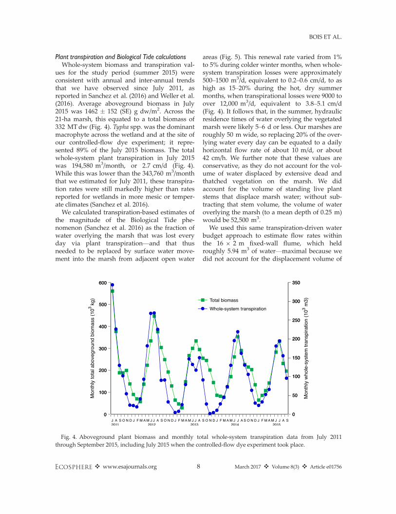
ues for the study period (summer 2015) wereconsistent with annual and inter-annual trendsthat we have observed since July 2011, asreported in Sanchez et al. (2016) and Weller et al.(2016). Average aboveground biomass in July2015 was 1462 � 152 (SE) g dw/m2. Across the21-ha marsh, this equated to a total biomass of332 MTdw (Fig. 4). Typha spp.was the dominantmacrophyte across the wetland and at the site ofour controlled-flow dye experiment; it repre-sented 89% of the July 2015 biomass. The totalwhole-system plant transpiration in July 2015was 194,580 m3/month, or 2.7 cm/d (Fig. 4).While this was lower than the 343,760 m3/monththat we estimated for July 2011, these transpira-tion rates were still markedly higher than ratesreported for wetlands in more mesic or temper-ate climates (Sanchez et al. 2016).

We calculated transpiration-based estimates ofthe magnitude of the Biological Tide phe-nomenon (Sanchez et al. 2016) as the fraction ofwater overlying the marsh that was lost everyday via plant transpiration—and that thusneeded to be replaced by surface water move-ment into the marsh from adjacent open water

areas (Fig. 5). This renewal rate varied from 1%to 5% during colder winter months, when whole-system transpiration losses were approximately500–1500 m3/d, equivalent to 0.2–0.6 cm/d, to ashigh as 15–20% during the hot, dry summermonths, when transpirational losses were 9000 toover 12,000 m3/d, equivalent to 3.8–5.1 cm/d(Fig. 4). It follows that, in the summer, hydraulicresidence times of water overlying the vegetatedmarsh were likely 5–6 d or less. Our marshes areroughly 50 m wide, so replacing 20% of the over-lying water every day can be equated to a dailyhorizontal flow rate of about 10 m/d, or about42 cm/h. We further note that these values areconservative, as they do not account for the vol-ume of water displaced by extensive dead andthatched vegetation on the marsh. We didaccount for the volume of standing live plantstems that displace marsh water; without sub-tracting that stem volume, the volume of wateroverlying the marsh (to a mean depth of 0.25 m)would be 52,500 m3.We used this same transpiration-driven water

budget approach to estimate flow rates withinthe 16 9 2 m fixed-wall flume, which heldroughly 5.94 m3 of water—maximal because wedid not account for the displacement volume of

Fig. 4. Aboveground plant biomass and monthly total whole-system transpiration data from July 2011through September 2015, including July 2015 when the controlled-flow dye experiment took place.


BOIS ET AL.

dead plant litter (wrack) or non-emergent aqua-tic vegetation (Hydrocotyl sp.). In July 2015, the32 m2 of marsh within the flume contained30.3 kg dw of Typha sp. biomass that transpired68 L/h (0.95 m3/d or 3.0 cm/d) of water (takinginto account 14 h of sunlight/d)—16% of themaximal volume of water within the flume. Toreplace this daily transpirational loss, new waterwould have had to flow into the flume at a rateof 2.57 m/d or 11 cm/h.

Dye experimentsConsidering that (1) the water flow cross sec-

tion within the flume was quite large comparedwith the tubing section of the autosampler and(2) the fixed walls of the flume were not impervi-ous at the bottom, it was clearly very difficult toachieve a high tracer mass recovery. Neither ahigh recovery rate, nor the knowledge of the fullRTD was the primary goal of this present work,though. We performed our calculations on thebasis of the obtained BTCs (available inAppendix S1), which represent the fraction of thetracer mass we recovered. We got around 1%mass recovery for Experiment 1 and between 4%and 12% mass recovery (around 12% for the 1-m,5% for the 3-m, and 4% for the 5-m samplingpoint) for Experiment 2. This low recovery ratehad no impact on the data analysis in this studyand the conclusions that are drawn, since the

BTCs at the different sampling points gave valu-able information.For Experiment 1, we only calculated maxi-

mum velocity (see Discussion). For Experiment 2,the dye peak progressed down the flume in apredictable way, demonstrating that water wasclearly, if slowly, advecting/dispersing into themarsh (Fig. 6). Additionally, the down-flumeprogression of the peak, from the marsh–openwater interface toward the shore, confirmed theexpected direction of water movement. In thefirst experiment, we calculated a high flow rate,200 cm/h or 48 m/d, at the 1-m sampling location(Table 2). Otherwise, maximum velocities forboth experiments ranged from 29 to 50 cm/h, or7 to 12 m/d. The precision for these values was5–8%. We found that the corresponding localmean velocities at the specific sampling pointsranged from 7 to 25 cm/h (Table 2). The resultingflume mean velocity for this experiment was16 cm/h, corresponding to 3.8 m/d.In addition to advection, water flow is also

characterized by dispersion and diffusion, and inlow-flow situations where there are obstacles toflow—such as our marsh—dispersion may be alarge component of flow. A simple measure ofdispersion is the degree to which the fluores-cence peaks widen and their tail increases withdistance—and thus time—from the injectionpoint. We found that the dispersion of the curves

Fig. 5. Monthly average (�SE) fraction of the water overlying the marsh that was transpired daily from July2011 through September 2015. Red circles represent months where transpiration was measured but could not betemporally scaled because of missing meteorological station data (see Sanchez et al. 2016 for details). Blue circlesrepresent the percentage of marsh water transpired daily.


BOIS ET AL.

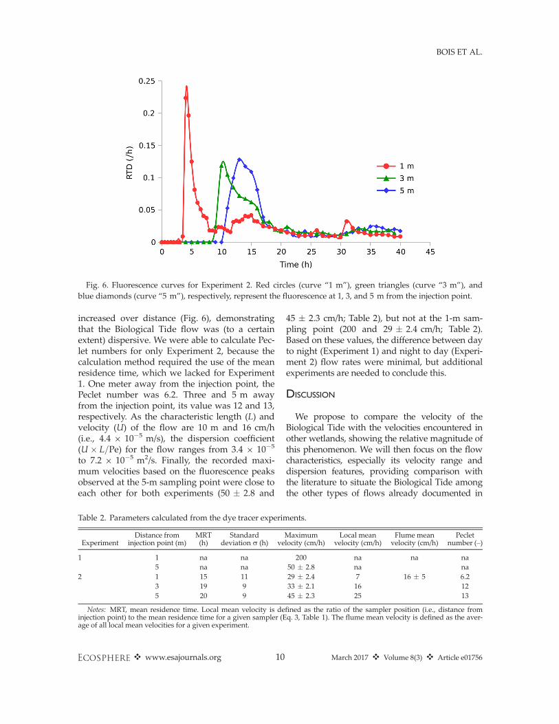
increased over distance (Fig. 6), demonstratingthat the Biological Tide flow was (to a certainextent) dispersive. We were able to calculate Pec-let numbers for only Experiment 2, because thecalculation method required the use of the meanresidence time, which we lacked for Experiment1. One meter away from the injection point, thePeclet number was 6.2. Three and 5 m awayfrom the injection point, its value was 12 and 13,respectively. As the characteristic length (L) andvelocity (U) of the flow are 10 m and 16 cm/h(i.e., 4.4 9 10�5 m/s), the dispersion coefficient(U � L=Pe) for the flow ranges from 3.4 9 10�5

to 7.2 9 10�5 m2/s. Finally, the recorded maxi-mum velocities based on the fluorescence peaksobserved at the 5-m sampling point were close toeach other for both experiments (50 � 2.8 and

45 � 2.3 cm/h; Table 2), but not at the 1-m sam-pling point (200 and 29 � 2.4 cm/h; Table 2).Based on these values, the difference between dayto night (Experiment 1) and night to day (Experi-ment 2) flow rates were minimal, but additionalexperiments are needed to conclude this.

DISCUSSION

We propose to compare the velocity of theBiological Tide with the velocities encountered inother wetlands, showing the relative magnitude ofthis phenomenon. We will then focus on the flowcharacteristics, especially its velocity range anddispersion features, providing comparison withthe literature to situate the Biological Tide amongthe other types of flows already documented in

Fig. 6. Fluorescence curves for Experiment 2. Red circles (curve “1 m”), green triangles (curve “3 m”), andblue diamonds (curve “5 m”), respectively, represent the fluorescence at 1, 3, and 5 m from the injection point.

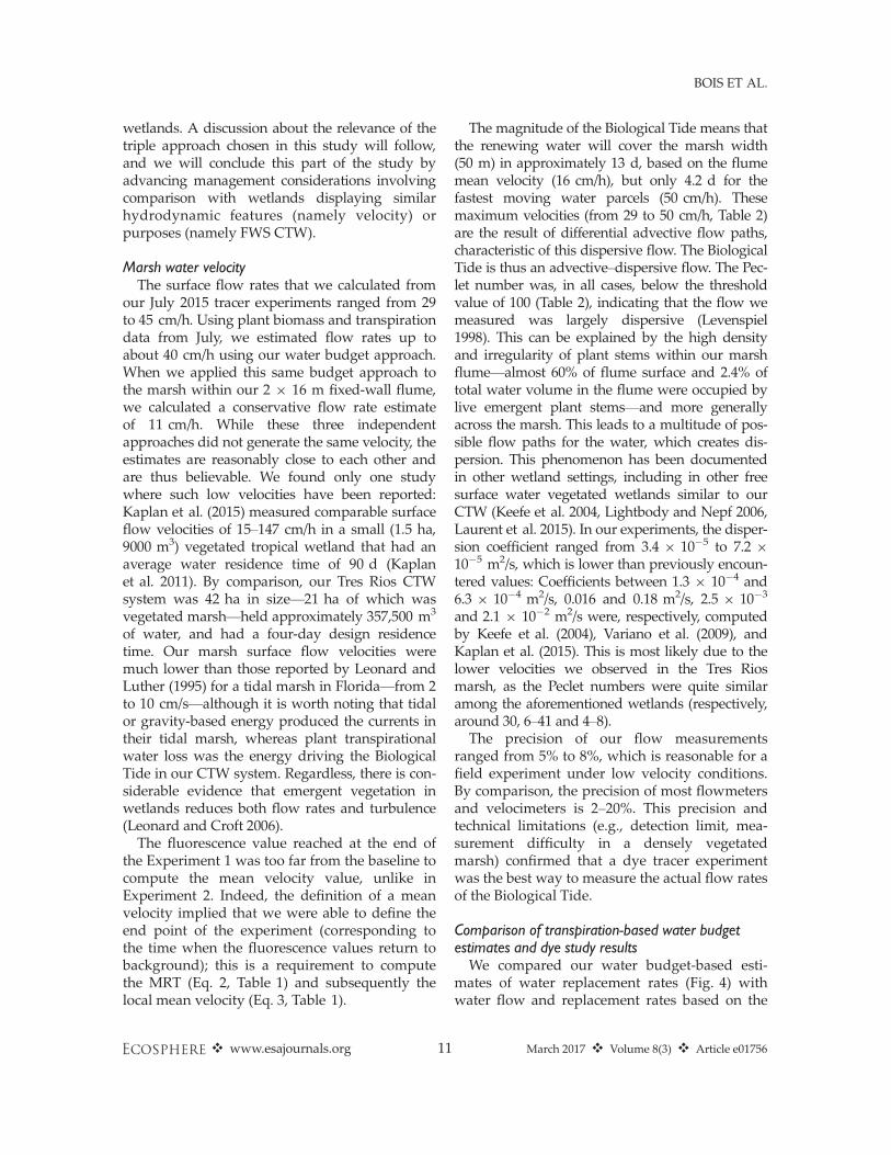
Table 2. Parameters calculated from the dye tracer experiments.

ExperimentDistance from

injection point (m)MRT(h)

Standarddeviation r (h)

Maximumvelocity (cm/h)

Local meanvelocity (cm/h)

Flume meanvelocity (cm/h)

Pecletnumber (–)

1 1 na na 200 na na na5 na na 50 � 2.8 na na

2 1 15 11 29 � 2.4 7 16 � 5 6.23 19 9 33 � 2.1 16 125 20 9 45 � 2.3 25 13

Notes: MRT, mean residence time. Local mean velocity is defined as the ratio of the sampler position (i.e., distance frominjection point) to the mean residence time for a given sampler (Eq. 3, Table 1). The flume mean velocity is defined as the aver-age of all local mean velocities for a given experiment.


BOIS ET AL.

wetlands. A discussion about the relevance of thetriple approach chosen in this study will follow,and we will conclude this part of the study byadvancing management considerations involvingcomparison with wetlands displaying similarhydrodynamic features (namely velocity) orpurposes (namely FWS CTW).

Marsh water velocityThe surface flow rates that we calculated from

our July 2015 tracer experiments ranged from 29to 45 cm/h. Using plant biomass and transpirationdata from July, we estimated flow rates up toabout 40 cm/h using our water budget approach.When we applied this same budget approach tothe marsh within our 2 9 16 m fixed-wall flume,we calculated a conservative flow rate estimateof 11 cm/h. While these three independentapproaches did not generate the same velocity, theestimates are reasonably close to each other andare thus believable. We found only one studywhere such low velocities have been reported:Kaplan et al. (2015) measured comparable surfaceflow velocities of 15–147 cm/h in a small (1.5 ha,9000 m3) vegetated tropical wetland that had anaverage water residence time of 90 d (Kaplanet al. 2011). By comparison, our Tres Rios CTWsystem was 42 ha in size—21 ha of which wasvegetated marsh—held approximately 357,500 m3

of water, and had a four-day design residencetime. Our marsh surface flow velocities weremuch lower than those reported by Leonard andLuther (1995) for a tidal marsh in Florida—from 2to 10 cm/s—although it is worth noting that tidalor gravity-based energy produced the currents intheir tidal marsh, whereas plant transpirationalwater loss was the energy driving the BiologicalTide in our CTW system. Regardless, there is con-siderable evidence that emergent vegetation inwetlands reduces both flow rates and turbulence(Leonard and Croft 2006).

The fluorescence value reached at the end ofthe Experiment 1 was too far from the baseline tocompute the mean velocity value, unlike inExperiment 2. Indeed, the definition of a meanvelocity implied that we were able to define theend point of the experiment (corresponding tothe time when the fluorescence values return tobackground); this is a requirement to computethe MRT (Eq. 2, Table 1) and subsequently thelocal mean velocity (Eq. 3, Table 1).

The magnitude of the Biological Tide means thatthe renewing water will cover the marsh width(50 m) in approximately 13 d, based on the flumemean velocity (16 cm/h), but only 4.2 d for thefastest moving water parcels (50 cm/h). Thesemaximum velocities (from 29 to 50 cm/h, Table 2)are the result of differential advective flow paths,characteristic of this dispersive flow. The BiologicalTide is thus an advective–dispersive flow. The Pec-let number was, in all cases, below the thresholdvalue of 100 (Table 2), indicating that the flow wemeasured was largely dispersive (Levenspiel1998). This can be explained by the high densityand irregularity of plant stems within our marshflume—almost 60% of flume surface and 2.4% oftotal water volume in the flume were occupied bylive emergent plant stems—and more generallyacross the marsh. This leads to a multitude of pos-sible flow paths for the water, which creates dis-persion. This phenomenon has been documentedin other wetland settings, including in other freesurface water vegetated wetlands similar to ourCTW (Keefe et al. 2004, Lightbody and Nepf 2006,Laurent et al. 2015). In our experiments, the disper-sion coefficient ranged from 3.4 9 10�5 to 7.2 9

10�5 m2/s, which is lower than previously encoun-tered values: Coefficients between 1.3 9 10�4 and6.3 9 10�4 m2/s, 0.016 and 0.18 m2/s, 2.5 9 10�3

and 2.1 9 10�2 m2/s were, respectively, computedby Keefe et al. (2004), Variano et al. (2009), andKaplan et al. (2015). This is most likely due to thelower velocities we observed in the Tres Riosmarsh, as the Peclet numbers were quite similaramong the aforementioned wetlands (respectively,around 30, 6–41 and 4–8).The precision of our flow measurements

ranged from 5% to 8%, which is reasonable for afield experiment under low velocity conditions.By comparison, the precision of most flowmetersand velocimeters is 2–20%. This precision andtechnical limitations (e.g., detection limit, mea-surement difficulty in a densely vegetatedmarsh) confirmed that a dye tracer experimentwas the best way to measure the actual flow ratesof the Biological Tide.

Comparison of transpiration-based water budgetestimates and dye study resultsWe compared our water budget-based esti-

mates of water replacement rates (Fig. 4) withwater flow and replacement rates based on the


BOIS ET AL.

controlled-flow dye study conducted in July 2015(Table 2). From transpiration calculations, weestimated a water velocity of 35–42 cm/h for a50 m wide marsh in mid-summer, and a waterresidence time of 5–6 d for the water overlyingthe marsh (Fig. 5). The Rhodamine dyeexperiments confirmed velocities ranging from25 cm/h (local mean velocity) to 45 cm/h (maxi-mum velocity). The coherence between these twoindependent flow rate calculations is strong. Asyet another methodological check, immediatelyafter the dye experiment ended we also mea-sured plant biomass and transpiration rates forthe marsh within the 2 9 16 m fixed-wall flumeitself, and used our water budget approach toestimate a replacement rate for the water in theflume. We estimated transpirational water losswithin the flume area as roughly 950 L/d, or (aconservatively calculated) 16% of the total watervolume within the flume. By extrapolation, weestimated that the rate of water flow that wouldbe needed to replace this 16% loss, if the flumewas closed at the downstream end, was 11 cm/h.This flume-specific water budget-based flow esti-mate is lower than, but still aligns reasonablywell with, both our long-term whole-systemtranspiration-based estimates and the actual flowrates that we measured from the controlled-flowdye study.

Management considerationsOur five years of research at the Tres Rios

CTW has documented that the most biogeo-chemically active zone of the system is the vege-tated marsh (Sanchez et al. 2016, Weller et al.2016). This is not surprising. But the manage-ment implications are important—if inorganicnitrogen, and presumably many other contami-nants, gets into the marsh proper, they are effec-tively removed from the water (Weller et al.2016). But the design water residence time for theentire 42-ha system, only 21 ha of which is vege-tated marsh, is only four days, and it is likelythat a considerable amount of the water enteringthe system leaves four days later without evercoming into contact with the biogeochemicallyactive marsh. The high rates of summer waterloss via plant transpiration, and the BiologicalTide that is being driven by this, move morewater and nitrogen into the marsh from the openwater areas than would happen in a similar

CTW in a cooler or more mesic climate. Thus, thebiotically mediated surface hydrologic phe-nomenon that we have documented here, for thefirst time, is actually increasing the effectivenessof this CTW, simply because it is located in a hot,dry climate. Because of this, we would recom-mend a design for CTW in hot arid climates thateither increases the relative area of vegetatedmarsh or increases the hydraulic likelihood thatany given parcel of water in the system will comeinto contact with vegetated marsh.Another design recommendation also focuses

on water residence time. To demonstrate thepotential importance of this hydraulic character-istic, we compared data from our CTW with sim-ilar values from a natural wetland located in thetropics (Costa Rica). The mean water residencetime in natural La Reserva wetland was 100 dcompared with 4 d in the Tres Rios CTW(Kaplan et al. 2011). This difference is largelybecause the water outflow rate at the latter wasmuch higher (Table 3). One could expect that thehigher water residence time in the La Reservawetland would result in a higher nutrient uptakeefficiency. However, the nitrogen removal effi-ciency of the La Reserva system (51–98.5%) wasonly double that of the Tres Rios CTW (22–48%,see Sanchez et al. 2016). If the Tres Rios CTWwas designed for a longer whole-system water

Table 3. Comparison of hydraulic characteristicsbetween a constructed treatment wetland (Tres Rios)and a natural wetland (La Reserva; Kaplan et al.2011, 2015).

Parameters TR LRTR/LRRatio

Average outflow(m3/h)

5000 6.25 � 3.31† 523–1700

Volume (m3) 351,500 7400–10,000† 35–48Whole-systemresidence time (d)

4 30–110† 0.036–0.13

Marsh velocity(cm/h)

16 25–110‡ 0.15–0.64

Marsh width (m) 50 – –Marsh residencetime (d)

13 100† 0.13

Note: TR, Tres Rios wetland; LR, La Reserva wetland.† Values from Kaplan et al. (2011). Intervals shown are

95% confidence intervals.‡ Values from Kaplan et al. (2015). The lowest value corre-

sponds to the wetland western average velocity; the highestone corresponds to the wetland eastern average velocity.


BOIS ET AL.

residence time, in conjunction with a physicaldesign that allowed for more water contact withthe vegetated marsh—and perhaps a highermarsh/open water ratio—we predict that itswhole-system nutrient uptake efficiency, whichis different from the marsh-specific uptake effi-ciency of nearly 100%, would be considerablyhigher.

Finally, in order to enlarge the comparisonwith systems sharing the same purpose andhydrological type, we put in perspective theremoval efficiency of our wetland with a litera-ture review of the removal performances of FWSCTWs (Kadlec and Wallace 2009). The reportedmean removal rates reach 60% for ammonia,with a mean hydraulic loading rate of 7.3 cm/h(N = 118), and 46% for nitrate, with a meanhydraulic loading rate of 11.4 cm/h (N = 72). Itthus appears that the Tres Rios CTW is fairly effi-cient, since the removal rates we measured reach48% for ammonia and 22% for nitrate (Sanchezet al. 2016), while the hydraulic loading rate isroughly four times higher—42.9 cm/h. We canhypothesize that the Biological Tide we con-firmed in the Tres Rios CTW, although not opti-mally utilized, already allows for significantnitrogen removal efficiency.

We are currently using a spatially articulatecell-based hydrodynamic model of the Tres RiosCTW, in conjunction with a biogeochemical pro-cessing model, to experiment with differenthypothetical design options for this and otherCTW systems.

Conclusions and next stepsWe have used more than six years of data on

plant community composition and biomass pro-duction, transpiration and evaporation rates, andwater quality to verify the efficacy of nitrogenremoval by the Tres Rios CTW. We have alsoused our whole-system water budget to demon-strate a plant-mediated, transpiration-driven Bio-logical Tide that brings new water and nitrogeninto the vegetated marsh of this CTW, where it iseffectively removed and processed (Sanchezet al. 2016, Weller et al. 2016). In the research wepresent here, we used an empirical controlled-flow tracer study to confirm not only the exis-tence and flow rates of the Biological Tide, but toverify the accuracy of our water budget-basedestimates of flow rates. As we noted above, this

is (to our knowledge) the first time that bioticcontrol of surface hydrology has ever beendemonstrated in a wetland ecosystem.Our next steps involve using numerical model-

ing to further articulate how the Biological Tidephenomenon is enhancing nutrient removal inthe wetlands of this CTW, and to explore designoptions for hypothetical CTW systems that opti-mize for this phenomenon. We are developingand parameterizing a spatially articulate hydro-dynamic model, based on the current design ofthe Tres Rios CTW, that accounts for actual waterflow rates between the marsh and open waterbodies and that accurately simulates whole-system water residence times. We will then usethis model to test various hypothetical design sce-narios, including (1) different ratios and configu-rations of marsh and open water, (2) differentopen water flow paths, including a scenariowhere all water entering the system must come incontact with vegetated marsh, (3) various macro-phyte community compositions, and (4) differentplant densities (Kjellin et al. 2007). Ultimately,these modeling exercises will inform both imp-roved management practices for the Tres RiosCTW and future designs that maximize the eco-system services provided by CTW “turquoise”infrastructure in aridland cities around the world.

ACKNOWLEDGMENTS

The first year of this work was supported by theU.S. Geological Survey through a grant from theArizona Water Resources Research Institute. Addi-tional support was provided by the National ScienceFoundation through the Central Arizona-PhoenixLong-Term Ecological Research Program (Grant No.1027188) and the Urban Sustainability Research Coor-dination Network (Grant No. 1140070). The WaltonSustainable Solutions Initiative at ASU funded collabo-rative travel between Phoenix and Strasbourg, includ-ing P. Bois’ travel in summer 2015. The Long-TermEcological Research Network from France and theStrasbourg Long-Term Ecological Research Program(ZAEU) funded P. Bois’ travel in summer 2014. Wethank Hilairy Hartnett and Joshua Nye at ASU for theuse of their fluorometer and lab space, Ben Warner forhis contributions early in the project, Nich Weller forleading the macrophyte data collection efforts for thefirst three years of the project, the City of PhoenixWater Services Department for their support and forproviding access to Tres Rios and key datasets, DakotaTallman for coordinating much of the research


BOIS ET AL.

conducted in 2013, and the many student volunteerswho helped with the field and laboratory work.

LITERATURE CITED

Bauer, P., G. Thabeng, F. Stauffer, and W. Kinzelbach.2004. Estimation of the evapotranspiration ratefrom diurnal groundwater level fluctuations in theOkavango Delta, Botswana. Journal of Hydrology288:344–355.

Bauer-Gottwein, P., T. Langer, H. Prommer, P. Wolski,and W. Kinzelbach. 2007. Okavango Delta Islands:interaction between density-driven flow and geo-chemical reactions under evapo-concentration.Journal of Hydrology 335:389–405.

Bazante, J., G. Jacobi, H. Solo-Gabriele, D. Reed,S. Mitchell-Bruker, D. L. Childers, L. Leonard, andM. Ross. 2006. Hydrologic measurements andimplications for tree island formation within Ever-glades National Park. Journal of Hydrology 329:606–619.

Bodin, H., A. Mietto, P. M. Ehde, J. Persson, and S. E.B. Weisner. 2012. Tracer behaviour and analysis ofhydraulics in experimental free water surfacewetlands. Ecological Engineering 49:201–211.

Bouma, T. J., L. A. van Duren, S. Temmerman,T. Claverie, A. Blanco-Garcia, T. Ysebaert, and P. M.J. Herman. 2007. Spatial flow and sedimentationpatterns within patches of epibenthic structures:combining field, flume and modelling experiments.Continental Shelf Research 27:1020–1045.

Bowmer, K. H. 1987. Nutrient removal from effluentsby an artificial wetland: influence of rhizosphereaeration and preferential flow studied using bro-mide and dye tracers. Water Research 21:591–597.

Chang, N. B., A. J. Crawford, G. Mohiuddin, andJ. Kaplan. 2015. Low flow regime measurementswith an automatic pulse tracer velocimeter (APTV)in heterogeneous aquatic environments. Flow Mea-surement and Instrumentation 42:98–112.

Childers, D. L. 1994. Fifteen years of marsh flumes—Areview of marsh-water column interactions inSoutheastern USA estuaries. Pages 277–296 inW. Mitsch, editor. Global wetlands. Elsevier, Ams-terdam, The Netherlands.

Childers, D. L., M. L. Cadenasso, J. M. Grove,V. Marshall, B. McGrath, and S. T. A. Pickett. 2015.An ecology for cities: a transformational nexus ofdesign and ecology to advance climate change resi-lience and urban sustainability. Sustainability 7:3774–3791.

Childers, D. L., and J. W. Day Jr. 1988. A flow-throughflume technique for quantifying nutrient and mate-rials fluxes in microtidal estuaries. Estuarine,Coastal and Shelf Science 27:483–494.

Childers, D. L., and J. W. Day Jr. 1990a. Marsh-watercolumn interactions in two Louisiana estuaries. I.Sediment dynamics. Estuaries 13:393–403.

Childers, D. L., and J. W. Day Jr. 1990b. Marsh-watercolumn interactions in two Louisiana estuaries. II.Nutrient dynamics. Estuaries 13:404–417.

Childers, D. L., D. Iwaniec, D. Rondeau, G. Rubio,E. Verdon, and C. Madden. 2006. Primaryproductivity in Everglades marshes demonstratesthe sensitivity of oligotrophic ecosystems to envi-ronmental drivers. Hydrobiologia 569:273–292.

Childers, D. L., S. T. A. Pickett, J. M. Grove, L. Ogden,and A. Whitmer. 2014. Advancing urban sustain-ability theory and action: challenges and opportu-nities. Landscape & Urban Planning 125:320–328.

Daoust, R., and D. L. Childers. 1998. Quantifyingaboveground biomass and estimating productivityin nine Everglades wetland macrophytes using anon-destructive allometric approach. Aquatic Bot-any 62:115–133.

Davis III, S. E., D. L. Childers, J. W. Day Jr., D. T.Rudnick, and F. H. Sklar. 2001a. Wetland-watercolumn exchanges of carbon, nitrogen, and phos-phorus in a Southern Everglades dwarf mangrove.Estuaries 24:610–622.

Davis III, S. E., D. L. Childers, J. W. Day Jr., D. T.Rudnick, and F. H. Sklar. 2001b. Nutrient dynamicsin vegetated and unvegetated areas of a southernEverglades mangrove creek. Estuarine, Coastaland Shelf Science 52:753–768.

Fonder, N., and T. Headley. 2010. Systematic classifica-tion, nomenclature, and reporting for constructedtreatment wetlands. Pages 191–219 in J. Vymazal,editor. Water and nutrient management in naturaland constructed wetlands. Springer Science + Busi-ness Media B.V., Dordrecht, The Netherlands.

Fonder, N., and T. Headley. 2013. The taxonomy oftreatment wetlands: a proposed classification andnomenclature system. Ecological Engineering 51:203–211.

Gendron, P. O., F. Avaltroni, and K. J. Wilkinson. 2008.Diffusion coefficients of several rhodamine deriva-tives as determined by pulsed field gradient-nuclear magnetic resonance and fluorescencecorrelation spectroscopy. Journal of Fluorescence18:1093–1101.

Giraldi, D., M. de’Michieli Vitturi, M. Zaramella,A. Marion, andR. Iannelli. 2009. Hydrodynamics ofvertical subsurface flow constructed wetlands:tracer tests with rhodamine WT and numericalmodeling. Ecological Engineering 35:265–273.

Greenway, M. 2005. The role of constructed wetlandsin secondary effluent treatment and water reuse insubtropical and arid Australia. Ecological Engi-neering 25:501–509.


BOIS ET AL.

Grimm, N. B., S. H. Faeth, N. E. Golubiewski, C. L.Redman, J. Wu, X. Bai, and J. M. Briggs. 2008.Global change and the ecology of cities. Science319:756–760.

Grove, J. M. 2009. Cities: managing densely settledsocial-ecological systems. Pages 281–294 in F. S.Chapin III, G. P. Kofinas, and C. Folke, editors.Principles of ecosystem stewardship: resilience-based natural resource management in a changingworld. Springer, New York, New York, USA.

Harvey, J. W., G. B. Noe, L. G. Larsen, D. J. Nowacki,and L. E. McPhillips. 2011. Field flume revealsaquatic vegetation’s role in sediment and particu-late phosphorus transport in a shallow aquaticecosystem. Geomorphology 126:297–313.

Kadlec, R. H., and S. D. Wallace. 2009. Treatmentwetlands. Second edition. CRC Press, Boca Raton,Florida, USA.

Kaplan, D., M. Bachelin, R. Munoz-Carpena, andW. Rodriguez-Chacon. 2011. Hydrological impor-tance and water quality treatment potential of asmall freshwater wetland in the humid tropics ofCosta Rica. Wetlands 31:1117–1130.

Kaplan, D., M. Bachelin, C. Yu, R. Munoz-Carpena,T. L. Potter, and W. Rodriguez-Chacon. 2015. Ahydrologic tracer study in a small, natural wetlandin the humid tropics of Costa Rica. Wetlands Ecol-ogy and Management 23:167–182.

Keefe, S. H., L. B. Barber, R. L. Runkel, J. N. Ryan,D. M. McKnight, and R. D. Wass. 2004. Conserva-tive and reactive solute transport in constructedwetlands. Water Resources Research 40:W01201.

Kjellin, J., A. Worman, H. Johansson, and A. Lindahl.2007. Controlling factors for water residence timeand flow patterns in Ekeby treatment wetland,Sweden. Advances in Water Resources 30:838–850.

Laurent, J., P. Bois, M. Nuel, and A. Wanko. 2015.Systemic models of full-scale Surface Flow Treat-ment Wetlands: determination by application offluorescent tracers. Chemical Engineering Journal264:389–398.

Leonard, L. A., and A. L. Croft. 2006. The effect ofstanding biomass on flow velocity and turbulencein Spartina alterniflora canopies. Estuarine, Coastaland Shelf Science 69:325–336.

Leonard, L. A., and M. E. Luther. 1995. Flow hydrody-namics in tidal marsh canopies. Limnology andOceanography 40:1474–1484.

Levenspiel, O. 1998. Chemical reaction engineering.Third edition. Wiley, New York, New York, USA.

Lightbody, A. F., and H. M. Nepf. 2006. Prediction ofvelocity profiles and longitudinal dispersion inemergent salt marsh vegetation. Limnology andOceanography 51:218–228.

McLaughlin, D. L., and M. J. Cohen. 2014. Ecosystemspecific yield for estimating evapotranspirationand groundwater exchange from diel surface watervariation. Hydrological Processes 28:1495–1506.

Melosi, M. V. 2000. The sanitary city: environmentalservices in urban America from colonial times tothe present. Johns Hopkins University Press, Balti-more, Maryland, USA.

Meselhe, E., T. Peeva, and M. Muste. 2004. Large scaleparticle image velocimetry for low velocity andshallow water flows. Journal of Hydraulic Engi-neering 130:937–940.

Metson, G., R. Hale, D. Iwaniec, E. Cook, J. Corman,C. Galletti, and D. Childers. 2012. Phosphorus inPhoenix: a budget and spatial representation ofphosphorus in an urban ecosystem. EcologicalApplications 22:705–721.

Nivala, J., T. Headley, S. Wallace, K. Bernhard, H. Brix,M. van Afferden, and R. A. M€uller. 2013. Compara-tive analysis of constructed wetlands: the designand construction of the ecotechnology researchfacility in Langenreichenbach, Germany. EcologicalEngineering 61:527–543.

Pickett, S. T. A., C. G. Boone, B. P. McGrath, M. L.Cadenasso, D. L. Childers, L. A. Ogden, M. McHale,and J. M. Grove. 2013. Ecological science andtransformation to the sustainable city. Cities 32:S10–S20.

Ramberg, L., and P. Wolski. 2008. Growing islands andsinking solutes: processes maintaining the endor-heic Okavango Delta as a freshwater system. PlantEcology 196:215–231.

Sanchez, C. A., D. L. Childers, L. Turnbull, R. Upham,and N. A. Weller. 2016. Aridland constructed treat-ment wetlands II: Plant mediation of surfacehydrology enhances nitrogen removal. EcologicalEngineering 97:658–665.

Smart, P. L., and I. M. S. Laidlaw. 1977. An evaluationof some fluorescent dyes for water. WaterResources Research 13:15–33.

Sullivan, P., R. M. Price, F. Miralles-Wilhelm, M. S.Ross, L. J. Scinto, T. W. Dreschel, F. H. Sklar,and E. Cline. 2014. The role of recharge and evapo-transpiration as hydraulic drivers of ion concentra-tions in shallow groundwater on Everglades treeislands, Florida (USA). Hydrological Processes 28:293–304.

Tanner, C. C., J. P. S. Sukias, T. R. Headley, C. R.Yates, and R. Stott. 2012. Constructed wetlands anddenitrifying bioreactors on-site and decentralizedwater treatment: comparison of five alternativeconfigurations. Ecological Engineering 42:112–123.

Troxler-Gann, T., and D. L. Childers. 2006. Relationshipsbetween hydrology and soils describe vegetation


BOIS ET AL.

patterns in tree seasonally flooded tree islands ofthe southern Everglades, Florida. Plant and Soil279:271–286.

Variano, E. A., D. T. Ho, V. C. Engel, P. J. Schmieder,C. Matthew, and M. C. Reid. 2009. Flow andmixing dynamics in a patterned wetland: kilome-ter-scale tracer releases in the Everglades. WaterResources Research 45:W08422.

Wallace, S. D., and R. L. Knight. 2006. Small-scaleconstructed wetland treatment systems: feasibility,design criteria, and O&M requirements. WaterEnvironment Research Foundation (WERF),Alexandria, Virginia, USA.

Weller, N. A., D. L. Childers, L. Turnbull, and R. F.Upham. 2016. Aridland constructed treatmentwetlands I: macrophyte productivity, community

composition, and nitrogen uptake. Ecological Engi-neering 97:649–657.

White, W. N. 1932. A method of estimating ground-water supplies based on discharge by plants andevaporation from soil: results of investigations inEscalante Valley, Utah. U.S. Geological SurveyWater Supply Paper: 659-A. U.S. Department of theInterior, Geological Survey, Washington, USA.

Williams, C. F., and S. D. Nelson. 2011. Comparison ofRhodamine-WT and bromide as a tracer for eluci-dating internal wetland flow dynamics. EcologicalEngineering 37:1492–1498.

Worman, W., and V. Kronnas. 2005. Effect of pondshape and vegetation heterogeneity on flow andtreatment performance of constructed wetlands.Journal of Hydrology 301:123–138.

SUPPORTING INFORMATION

Additional Supporting Information may be found online at: http://onlinelibrary.wiley.com/doi/10.1002/ecs2.1756/full


BOIS ET AL.

http://onlinelibrary.wiley.com/doi/10.1002/ecs2.1756/full

http://onlinelibrary.wiley.com/doi/10.1002/ecs2.1756/full

confirming a plant‐mediated …¬rming a plant-mediated “biological tide” in an aridland...

Documents