confidence limits for the indirect effect: distribution of

MULTIVARIATE BEHAVIORAL RESEARCH 99

Multivariate Behavioral Research, 39 (1), 99-128Copyright © 2004, Lawrence Erlbaum Associates, Inc.

Confidence Limits for the Indirect Effect:Distribution of the Product and Resampling Methods

David P. MacKinnon, Chondra M. Lockwood, and Jason WilliamsArizona State University

The most commonly used method to test an indirect effect is to divide the estimate of theindirect effect by its standard error and compare the resulting z statistic with a critical valuefrom the standard normal distribution. Confidence limits for the indirect effect are alsotypically based on critical values from the standard normal distribution. This article usesa simulation study to demonstrate that confidence limits are imbalanced because thedistribution of the indirect effect is normal only in special cases. Two alternatives forimproving the performance of confidence limits for the indirect effect are evaluated: (a) amethod based on the distribution of the product of two normal random variables, and (b)resampling methods. In Study 1, confidence limits based on the distribution of the productare more accurate than methods based on an assumed normal distribution but confidencelimits are still imbalanced. Study 2 demonstrates that more accurate confidence limits areobtained using resampling methods, with the bias-corrected bootstrap the best methodoverall.

An indirect effect implies a causal hypothesis whereby an independentvariable causes a mediating variable which, in turn, causes a dependentvariable (Sobel, 1990). Hypotheses regarding indirect or mediated effectsare implicit in social science theories (Alwin & Hauser, 1975; Baron &Kenny, 1986; Hyman, 1955; Sobel, 1982). Examples of indirect effecthypotheses are that attitudes affect intentions which then affect behavior(Ajzen & Fishbein, 1980), that poverty reduces local social ties whichincreases assault and burglary rates (Warner & Rountree, 1997), that socialstatus has an indirect effect on depression through changes in social stress(Turner, Wheaton, & Lloyd, 1995), and that father’s education affectsoffspring education which then affects offspring income (Duncan,Featherman, & Duncan, 1972).

This research was supported by the National Institute on Drug Abuse grant number 1R01 DA09757. We acknowledge the contributions of Ghulam Warsi and Jeanne Hoffmanto the work described in this article. We thank William Meeker, Leona Aiken, MichaelSobel, Steve West, and Jenn-Yun Tein for comments on an earlier version of thismanuscript.

Correspondence concerning this article should be addressed to David P. MacKinnon,Department of Psychology, Arizona State University, Tempe, AZ 85287-1104.

D. MacKinnon, C. Lockwood, and J. Williams

100 MULTIVARIATE BEHAVIORAL RESEARCH

Analysis of indirect effects is also important for experimental studies ofsocial policy interventions. Substance abuse prevention programs, forexample, are designed to change mediating variables such as social bonding(Hawkins, Catalano, & Miller, 1992) and social influence (Bandura, 1977)which are hypothesized to be causally related to drug abuse (see also Hansen& Graham, 1991, and Tobler, 1986, for more examples). In these contexts,the randomization of participants to treatment conditions and the knowledgethat the treatment precedes both the mediating variable and the dependentvariable in time strengthen the causal inferences that may be drawn aboutthe indirect effects of the intervention (Holland, 1988; Sobel, 1998). In theseexperimental studies, analysis of indirect effects (also called mediationanalysis) provides a check on whether the manipulation changed thevariables it was designed to change, tests theory by providing information onthe process through which the experiment changed the dependent variable,and generates information that may improve programs (MacKinnon, 1994;West & Aiken, 1997). Thus, the accuracy of confidence limits for theindirect effect is important for both basic and applied researchers in severalsubstantive areas of social science (Allison, 1995a; Bollen & Stine, 1990;Sobel, 1982).

Prior research provides much information on the relative performance ofvarious methods for conducting significance tests for indirect effects(MacKinnon, Lockwood, Hoffman, West, & Sheets, 2002), but very littleinformation about confidence limits. Confidence limit estimation has beenadvocated for several reasons, including that it forces researchers toconsider the size of an effect in addition to making a binary decision regardingsignificance and that the width of the interval provides a clearerunderstanding of variability in the size of the effect (Harlow, Mulaik, &Steiger, 1997; Krantz, 1999). The purpose of this article is to explain whythe traditional method used to test the significance of the indirect effectbased on the assumption of the z distribution has statistical power and TypeI error rates that are too low and imbalanced confidence limits. Twoalternatives to address the problem are evaluated in this article, one basedon the distribution of the product of two normal random variables and anotherbased on resampling methods. First, the equations used to estimate theindirect effect and its standard error are described, followed by evidence thattraditional confidence limits for the indirect effect are imbalanced. Next, anoverview of the distribution of the product is given with a description of howthis distribution explains inaccuracies in the traditional test of the indirecteffect. In Study 1, confidence limits for the traditional and distribution of theproduct methods are compared in a statistical simulation. In Study 2, asimulation study compares the distribution of the product method evaluated



in Study 1 with resampling methods which should also adjust for thenonnormal distribution of the indirect effect.

Estimation of the Indirect Effect and Standard Error

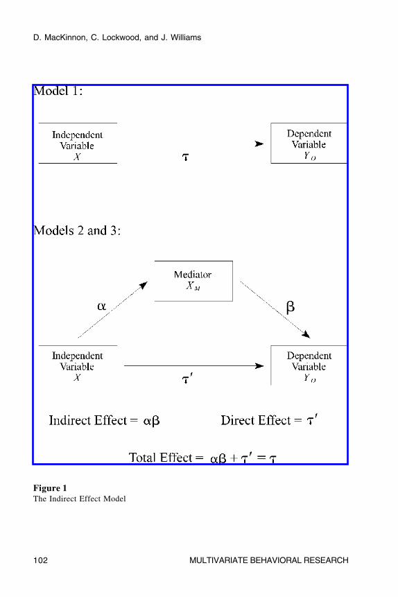
The indirect effect model is shown in Figure 1 and is summarized in thethree equations described below (see also Allison, 1995a and MacKinnon &Dwyer, 1993). We focus on a recursive model with a single indirect effectand ordinary regression models in order to more clearly describe theapproach.

(1) YO = �

01 + �X + ε

1

(2) YO = �

02 + ��X + �X

M + ε

2

(3) XM = �

03 + �X + ε

3

In these equations, YO is the dependent variable, X

is the independent variable,

XM is the mediating variable, � codes the relation between the independent

variable and the dependent variable, �� codes the relation between theindependent variable and the dependent variable adjusted for the effects ofthe mediating variable, � codes the relation between the independentvariable and the mediating variable, and � codes the relation between themediating variable and the dependent variable adjusted for the independentvariable. The residuals are coded by ε

1, ε

2, and ε

3 and the intercepts are

coded by �01

, �02

, and �03

in Equations 1, 2, and 3, respectively. The residualshave expected values of zero.

In the first regression equation, the dependent variable (YO) is regressed

on only the independent variable (X). In the second regression equation, thedependent variable (Y

O) is regressed on both the independent variable (X)

and the mediating variable (XM). The indirect effect equals the difference

in the estimated independent variable coefficients ( )ˆ ˆ� �′− in the tworegression equations (Judd & Kenny, 1981).

A second method to calculate the indirect effect is illustrated in Figure 1.First, the coefficient relating the mediating variable to the dependent variableis estimated ( � ) in Equation 2 above. Second, the coefficient relating theindependent variable to the mediating variable is estimated ( � ) in Equation3. The product of these two estimates ( � � ) is the estimated indirect effect.The estimated coefficient relating the independent variable to the dependentvariable adjusted for the mediating variable ( �′ ) is the estimate of the directeffect. The ˆ ˆ� �′− and � � estimators of the indirect effect are equivalent



Figure 1The Indirect Effect Model

http://www.leaonline.com/action/showImage?doi=10.1207%2Fs15327906mbr3901_4&iName=master.img-000.png&w=341&h=411



in ordinary least squares regression (MacKinnon, Warsi, & Dwyer, 1995).Additional assumptions of the � � estimator of the indirect effect fromEquations 2 and 3 have been outlined (James & Brett, 1984; McDonald,1997). These assumptions include no measurement error in variables (Hoyle& Kenny, 1999), the causal relations of X to M to Y are correct (McDonald,1997), no omitted variables (McDonald, 1997), and a zero interaction of Xand X

M (Judd & Kenny, 1981). The same assumptions are made for the

indirect effect model examined in this article.Although there are several estimators of the variance of the indirect

effect (see MacKinnon et al., 2002), the most commonly used estimator wasderived by Sobel (1982; 1986). This formula (Equation 4), based on themultivariate delta method, is used to calculate the standard error of theindirect effect in statistical software packages, including EQS (Bentler,1997), LISREL (Jöreskog & Sörbom, 1993), and LINCS (Schoenberg &Arminger, 1996), and is based on the estimates � and � , and the estimatedstandard errors, ˆˆ �� and ˆˆ

�� . Allison (1995a) used a reduced form

parameterization of the indirect effect model to derive the same standarderror formula in Equation 4. The formula assumes that � and � areindependent (Sobel, 1987). This variance estimator can be used to calculatestandard errors and confidence limits for the indirect effect. MacKinnon andDwyer (1993) and MacKinnon et al. (1995, 2002) found evidence that themultivariate delta method standard error had the least bias of severalformulas for the standard error of the indirect effect.

(4) 2 2 2 2 2ˆ ˆ ˆˆ

ˆˆ ˆ ˆ ˆ �� = +

For nonzero values of both � and �, simulation studies suggest that the varianceestimator has relative bias less than 5% for sample sizes of 100 or more in a singleindirect effect model (MacKinnon et al., 1995) and for sample sizes of 200 ormore in a recursive model with seven total indirect effects (Stone & Sobel, 1990).

In many studies, the indirect effect is divided by its standard error andthe resulting ratio is then compared to the standard normal distribution to testits significance, z = ˆˆ

ˆˆ ˆ/��

�� (Bollen & Stine, 1990; MacKinnon et al., 1991;Wolchik, Ruehlman, Braver, & Sandler, 1989). Confidence limits for theindirect effect lead to the same conclusion with regard to the null hypothesis.Confidence limits are constructed using Equation 5,

(5)ˆ1 / 2 ˆ

ˆˆ ˆ*z � �� −±

where z1 - �/2

is the value on the standard normal distribution correspondingto the desired Type I error rate, �.



Although the variance and standard error estimators of the indirecteffect may be unbiased at small sample sizes, there is evidence thatconfidence limits based on these values do not perform well. Two extensivesimulation studies (MacKinnon et al., 1995; Stone & Sobel, 1990) showed animbalance in the number of times a true value fell to the left or right of theconfidence limits. For positive values of the indirect effect, where � and �are both positive or both negative, the true value was more often to the rightthan to the left of the confidence interval. Asymmetric confidence intervalswere also obtained in bootstrap analysis of the indirect effect (Bollen &Stine, 1990; Lockwood & MacKinnon, 1998). The implication of theimbalance is that there is less power than expected to detect a true indirecteffect. Stone and Sobel (1990, p. 349) analytically demonstrated that at leastpart of the imbalance may be due to use of only first order derivatives in thesolution for the multivariate delta standard error of the indirect effect.However, MacKinnon et al. (1995) found that the second order Taylor seriessolution had similar imbalances in confidence intervals. Bollen and Stine(1990) noted that the asymptotic solutions for the standard error of theindirect effect may be incorrect for small sample sizes and used abootstrapping approach to improve the accuracy of confidence limits for theindirect effect. An explanation for the low power and imbalance inconfidence limits is the assumption that the distribution of the indirect effectis normal when, in fact, it is skewed for nonzero indirect effects and hasdifferent values of kurtosis for different values of the indirect effect, as willbe described in the next section.

The Distribution of the Product

The assumption that the indirect effect divided by its standard error hasa normal sampling distribution is incorrect in some situations. In thesesituations, the confidence limits calculated using Equation 5 will be incorrect.Because the indirect effect is the product of regression estimates which arenormally distributed asymptotically (Hanushek & Jackson, 1977), analternative method for testing indirect effects can be developed based on thedistribution of the product of two normally distributed random variables(Aroian, 1947; Craig, 1936; Springer, 1979).

The product of two normal random variables is not normally distributed(Lomnicki, 1967; Springer & Thompson, 1966). In the null case where bothrandom variables have means equal to zero, the distribution is symmetric withkurtosis of six (Craig, 1936). When the product of the means of the tworandom variables is nonzero, the distribution is skewed as well as havingexcess kurtosis, although Aroian (1947) and Aroian, Taneja, and Cornwell



(1978) showed that the product approaches the normal distribution as one orboth of the ratios of the means to standard errors of each random variableget large in absolute value. The four moments of the product of twocorrelated normal variables are given in Craig (1936), Aroian et al. (1978),and Meeker, Cornwell, and Aroian (1981).

The general analytical solution for the distribution of the product of twoindependent standard normal variables does not approximate distributionscommonly used in statistics, although Aroian (1947) showed that the gammadistribution can provide an approximation in some situations. Instead, theanalytical solution for this product distribution is a Bessel function of thesecond kind with a purely imaginary argument (Aroian, 1947; Craig, 1936).Although computation of these values is complex, Springer and Thompson(1966) provided a table of the values of this function when � = � = 0. Meekeret al. (1981; see pages 129-144 for uncorrelated variables) presented tablesof the distribution of the product of two normal random variables based onan alternative formula more conducive to numerical integration. Tables offractiles of the standardized distribution function for

ˆˆ

ˆˆ

��

��

�

−

for different values of �, �, ��

, and �� were given in Meeker et al. (1981).

The denominator was the exact standard error (Aroian, 1947; MacKinnon etal., 2002). Table entries were in terms of the ratio of each of the twovariables to their standard error so for � and �, the table entriescorresponded to �

� = �/�

� and �

� = �/�

�. Note that sample values of �

� and

�� correspond to the t-values for each regression coefficient. The critical

values in the table assume that population values of �, �, ��, and �

� are

known, but the authors suggest that sample values can be used in place ofthe population values as an approximation (Meeker et al., 1981, p. 8).

The frequency distribution function of the product of two standardizednormal variables, presented in Meeker et al. (1981), can be used to computethe statistical power, Type I error, and confidence limits for the indirecteffect. The test based on the tables in Meeker et al. is represented by M inthis article. In this method, the two estimated � statistics, one for the �estimate, ˆ

�� , and another for the � estimate, ˆ�� , are computed and used to

look up critical values in the table of critical values in Meeker et al. (1981).For example, the critical values of the M distribution for �

� = 0 and �

� = 0 (a

symmetric distribution) for two-tailed tests are 3.60, 2.18, and 1.60 fornominal Type I error rates of 0.01, 0.05, and 0.10, respectively.



The confidence limits based on the distribution of the product usingEquation 5 require different critical values for the upper (UCL) and lower(LCL) confidence limits because the distribution of the product of twonormal random variables can be asymmetric and depends on the values of�

� and �

�. The critical values are read from tables in Meeker et al. (1981)

based on values of ˆ�� and ˆ

�� and Equations 6 and 7 are used to computethe upper and lower confidence limits, respectively. This test is called theasymmetric distribution of the product test in MacKinnon et al. (2002).

(6) UCL = � � + Meeker Upper * ˆˆˆ��

�

(7) LCL = � � + Meeker Lower * ˆˆˆ��

�

The critical values are obtained from the tables in Meeker et al. (1981) whereMeeker Upper is the critical value for the upper confidence limit and MeekerLower is the critical value for the lower confidence limit. For example, the95% confidence interval for �

� = .4 and �

� = 1.2 would be calculated using

a Meeker Upper critical value of 2.3774 (p. 141) and a Meeker Lowercritical value of -1.8801 (p. 131).

Study 1

As described above, there is evidence that the traditional z test of theindirect effect has imbalanced confidence limits. The purpose of Study 1 isto compare the traditional z test to an approach based on the distribution ofthe product of two normal random variables in a large statistical simulationstudy.

Methods

Simulation Description

The SAS® (1989) programming language was used to conduct thestatistical simulations. The data were simulated using Equations 2 and 3, withsample values of X, ε

2, and ε

3 generated from a standard normal distribution

using the SAS RANNOR function with current time as the seed for eachsimulation. Five different sample sizes corresponding to sample sizes in thesocial sciences were simulated: 50, 100, 200, 500, and 1000. The independentvariable was simulated to be a normally distributed continuous variable. Asimulation study with a binary independent variable led to the same resultsas for the continuous independent variable case, so they are not described in



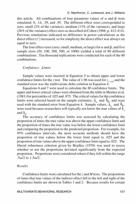
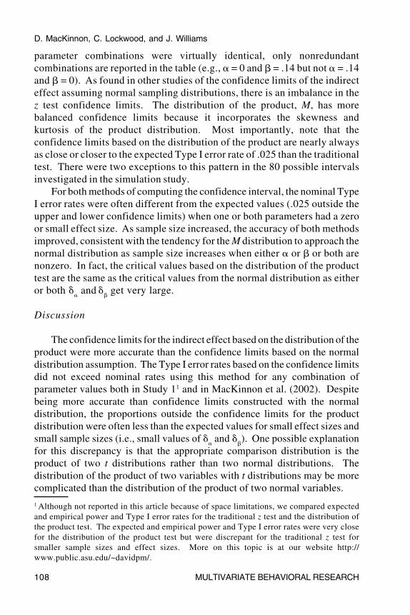
this article. All combinations of four parameter values of � and � weresimulated: 0, .14, .39, and .59. The different effect sizes corresponded tozero, small (2% of the variance), medium (13% of the variance), and large(26% of the variance) effect sizes as described in Cohen (1988, p. 412-414).Previous simulations indicated no difference in power calculations as thedirect effect (��) increased, so for simplicity the direct effect was always setequal to zero.

The four effect sizes (zero, small, medium, or large) for � and �, and fivesample sizes (50, 100, 200, 500, or 1000) yielded a total of 80 differentcombinations. Ten thousand replications were conducted for each of the 80combinations.

Confidence Limits

Sample values were inserted in Equation 5 to obtain upper and lowerconfidence limits for the z test. The value of 1.96 was used for z

1 - �/2 and the

standard error was the multivariate delta solution in Equation 4.Equations 6 and 7 were used to calculate the M confidence limits. The

upper and lower critical values were obtained from the table in Meeker et al.(1981) for percentiles of .025 and .975. The critical values for the confidencelimits were selected based on the sample estimates, ˆ

�� and ˆ�� , and were

used with the standard error from Equation 4. Sample values, ˆ�� and ˆ

�� ,were used because researchers will typically not know the true values of �

�

and ��.

The accuracy of confidence limits was assessed by calculating theproportion of times the true value was above the upper confidence limit andthe proportion of times the true value was below the lower confidence limitand comparing the proportion to the predicted proportion. For example, for95% confidence intervals, the most accurate methods should have theproportion of true values below the lower limit equal to .025 and theproportion of true values above the upper confidence limit equal to .025. Theliberal robustness criterion given by Bradley (1978) was used to assesswhether or not the proportions deviated significantly from the expectedproportion. Proportions were considered robust if they fell within the range.5�/2 to 1.5�/2.

Results

Confidence limits were calculated for the z and M tests. The proportionsof times that true values of the indirect effect fell to the left and right of theconfidence limits are shown in Tables 1 and 2. Because results for certain



parameter combinations were virtually identical, only nonredundantcombinations are reported in the table (e.g., � = 0 and � = .14 but not � = .14and � = 0). As found in other studies of the confidence limits of the indirecteffect assuming normal sampling distributions, there is an imbalance in thez test confidence limits. The distribution of the product, M, has morebalanced confidence limits because it incorporates the skewness andkurtosis of the product distribution. Most importantly, note that theconfidence limits based on the distribution of the product are nearly alwaysas close or closer to the expected Type I error rate of .025 than the traditionaltest. There were two exceptions to this pattern in the 80 possible intervalsinvestigated in the simulation study.

For both methods of computing the confidence interval, the nominal TypeI error rates were often different from the expected values (.025 outside theupper and lower confidence limits) when one or both parameters had a zeroor small effect size. As sample size increased, the accuracy of both methodsimproved, consistent with the tendency for the M distribution to approach thenormal distribution as sample size increases when either � or � or both arenonzero. In fact, the critical values based on the distribution of the producttest are the same as the critical values from the normal distribution as eitheror both �

� and

�

� get very large.

Discussion

The confidence limits for the indirect effect based on the distribution of theproduct were more accurate than the confidence limits based on the normaldistribution assumption. The Type I error rates based on the confidence limitsdid not exceed nominal rates using this method for any combination ofparameter values both in Study 11 and in MacKinnon et al. (2002). Despitebeing more accurate than confidence limits constructed with the normaldistribution, the proportions outside the confidence limits for the productdistribution were often less than the expected values for small effect sizes andsmall sample sizes (i.e., small values of �

� and �

�). One possible explanation

for this discrepancy is that the appropriate comparison distribution is theproduct of two t distributions rather than two normal distributions. Thedistribution of the product of two variables with t distributions may be morecomplicated than the distribution of the product of two normal variables.

1 Although not reported in this article because of space limitations, we compared expectedand empirical power and Type I error rates for the traditional z test and the distribution ofthe product test. The expected and empirical power and Type I error rates were very closefor the distribution of the product test but were discrepant for the traditional z test forsmaller sample sizes and effect sizes. More on this topic is at our website http://www.public.asu.edu/~davidpm/.



Tab

le 1

Pro

port

ion

of T

rue

Val

ues

to L

eft

and

Rig

ht o

f 95

% C

onfi

denc

e In

terv

als

- O

ne o

r T

wo

Zer

o P

aths

, S

tudy

1

Sam

ple

Siz

e

Eff

ect

Siz

e50

100

200

500

1000

��

Tes

ttr

ue t

otr

ue t

otr

ue t

otr

ue t

otr

ue t

otr

ue t

otr

ue t

otr

ue t

otr

ue t

otr

ue t

ole

ftri

ght

left

righ

tle

ftri

ght

left

righ

tle

ftri

ght

00

z0*

0.00

01*

0*0*

0*0.

0001

*0.

0002

*0*

0.00

03*

0*M

0.00

07*

0.00

09*

0.00

12*

0.00

09*

0.00

13*

0.00

05*

0.00

13*

0.00

07*

0.00

12*

0.00

06*

0.1

4z

0.00

03*

0.00

01*

0.00

13*

0.00

08*

0.00

23*

0.00

22*

0.00

64*

0.00

46*

0.01

290.

0127

M0.

0024

*0.

0018

*0.

0063

*0.

0040

*0.

0079

*0.

0079

*0.

0079

*0.

0140

0.01

940.

0190

0.3

9z

0.00

47*

0.00

42*

0.01

16*

0.00

78*

0.02

010.

0177

0.02

180.

0249

0.02

560.

0241

M0.

0129

0.01

22*

0.01

530.

0165

0.02

140.

0201

0.02

280.

0235

0.02

490.

0244

0.5

9z

0.01

260.

0119

*0.

0189

0.01

690.

0211

0.02

130.

0266

0.02

320.

0248

0.02

44M

0.02

020.

0179

0.02

050.

0181

0.02

110.

0215

0.02

630.

0223

0.02

480.

0241

Ave

rage

z0.

0044

*0.

0041

*0.

0080

*0.

0064

*0.

0109

*0.

0103

*0.

0138

0.01

320.

0159

0.01

53M

0.00

91*

0.00

82*

0.01

08*

0.00

99*

0.01

290.

0125

0.01

460.

0151

0.01

760.

0170

Not

e. z

ref

ers

to c

onfi

denc

e li

mit

s ba

sed

on t

he t

radi

tion

al z

tes

t.

M r

efer

s to

the

con

fide

nce

lim

its

form

ed b

ased

on

the

dist

ribu

tion

of

the

prod

uct

tabl

es i

n M

eeke

r et

al.

(19

81).

V

alue

s m

arke

d w

ith

* ar

e ou

tsid

e B

radl

ey (

1978

) ro

bust

ness

cri

teri

a.



Tab

le 2

Pro

port

ion

of T

rue

Val

ues

to L

eft

and

Rig

ht o

f 95

% C

onfi

denc

e In

terv

als

- N

o Z

ero

Pat

hs,

Stu

dy 1

Sam

ple

Siz

e

Eff

ect

Siz

e50

100

200

500

1000

��

Tes

ttr

ue t

otr

ue t

otr

ue t

otr

ue t

otr

ue t

otr

ue t

otr

ue t

otr

ue t

otr

ue t

otr

ue t

ole

ftri

ght

left

righ

tle

ftri

ght

left

righ

tle

ftri

ght

.14

.14

z0.

0006

*0.

0464

*0.

0019

*0.

0883

*0.

0040

*0.

0906

*0.

0070

*0.

0669

*0.

0112

*0.

0533

*M

0.00

64*

0.04

20*

0.00

98*

0.07

75*

0.01

330.

0830

*0.

0177

0.04

29*

0.01

890.

0362

.14

.39

z0.

0037

*0.

0521

*0.

0062

*0.

0451

*0.

0098

*0.

0430

*0.

0138

0.03

520.

0191

0.03

19M

0.01

340.

0464

*0.

0177

0.03

85*

0.01

980.

0384

*0.

0208

0.02

940.

0204

0.03

00.1

4.5

9z

0.00

72*

0.03

400.

0115

*0.

0347

0.01

720.

0311

0.01

890.

0269

0.02

190.

0280

M0.

0165

0.03

220.

0230

0.03

080.

0258

0.02

960.

0195

0.02

590.

0219

0.02

80.3

9.3

9z

0.00

62*

0.07

52*

0.01

09*

0.05

77*

0.01

21*

0.04

67*

0.01

580.

0369

0.01

650.

0340

M0.

0165

0.05

59*

0.01

920.

0410

*0.

0190

0.03

340.

0197

0.02

690.

0166

0.03

05.3

9.5

9z

0.00

89*

0.05

71*

0.01

04*

0.04

71*

0.01

460.

0404

*0.

0186

0.03

180.

0195

0.03

18M

0.01

930.

0417

*0.

0183

0.03

530.

0222

0.02

920.

0187

0.02

930.

0195

0.03

18.5

9.5

9z

0.00

94*

0.05

37*

0.01

370.

0435

*0.

0152

0.04

14*

0.01

680.

0307

0.02

110.

0300

M0.

0197

0.03

81*

0.02

190.

0331

0.01

850.

0318

0.01

680.

0293

0.02

110.

0300

Ave

rage

z0.

0060

*0.

0531

*0.

0091

*0.

0527

*0.

0122

*0.

0489

*0.

0152

0.03

81*

0.01

820.

0348

M0.

0153

0.04

27*

0.01

830.

0427

*0.

0198

0.04

09*

0.01

890.

0306

0.01

970.

0311

Not

e. z

ref

ers

to c

onfi

denc

e li

mit

s ba

sed

on t

he t

radi

tion

al z

tes

t.

M r

efer

s to

the

con

fide

nce

lim

its

form

ed b

ased

on

the

dist

ribu

tion

of

the

prod

uct

tabl

es i

n M

eeke

r et

al.

(19

81).

V

alue

s m

arke

d w

ith

* ar

e ou

tsid

e B

radl

ey (

1978

) ro

bust

ness

cri

teri

a.



The inaccuracy of some confidence limits based on the distribution of theproduct may also be due to the combination of the sampling variability of �

�

and �� and the different shape of the distribution of the product for each

different combination of �� and �

�. For example, when the true population

� is zero, the sample �� is commonly nonzero owing to sampling variability.

Because the shape of the distribution of the product changes depending onthe value of �

�, the confidence limits are subject to sampling variability.

Nevertheless, even with sample values of �� and �

�, the confidence limits

based on the distribution of the product were more accurate than the methodbased on a normal distribution for the indirect effect.

Resampling approaches may yield more accurate confidence limits andalso provide a test of the significance of the indirect effect (Manly, 1997;Noreen, 1989). The bootstrap resampling procedure is one method that mayprovide more accurate confidence limits (Bollen & Stine, 1990), but Type Ierror rates based on the standard percentile bootstrap approach are alsolower than predicted for small values of �

� and �

� (Lockwood & MacKinnon,

1998). The purpose of Study 2 is to evaluate several resampling methodsthat may yield more accurate confidence limits.

Study 2

In Study 1, although confidence limits for the indirect effect were moreaccurate when the distribution of the product was taken into account, therewere still cases where the number of times that the true value was outsidethe range of the confidence limits was smaller than expected. For example,the proportion outside the range for the case with � = 0 and � = 0 was muchlower than .025 for 95% confidence limits.

Several researchers have suggested that resampling methods such asthe jackknife and the bootstrap may provide more accurate tests of theindirect effect (Bollen & Stine, 1990; Lockwood & MacKinnon, 1998;Shrout & Bolger, 2002). Bollen and Stine (1990) found that bootstrapconfidence limits for the indirect effect were asymmetric. Lockwood andMacKinnon (1998) also obtained asymmetric confidence limits andpresented a computer program to conduct the bootstrap confidenceintervals for the indirect effect. Most recently, Shrout and Bolger (2002)recommended bootstrap methods to assess mediation for small to moderatesample sizes. Resampling methods are generally considered the method ofchoice when the assumptions of classical statistical methods are not met(Manly, 1997; Rodgers, 1999), such as for the nonnormal distribution of theindirect effect. Thus the purpose of Study 2 was to determine whetherjackknife, Monte Carlo, and bootstrap resampling methods yield more



accurate confidence limits for the indirect effect than single samplemethods used in Study 1.

Methods

Simulation Description

The simulation procedure in Study 1 was used in Study 2 with fourexceptions: sample size, parameter combinations, number of replications,and resampling methods. First, only four sample sizes were simulated: 25,50, 100, and 200. Because resampling methods are particularly useful whensample sizes are small, the two largest sample sizes from Study 1 weredropped and a sample size of 25 was added. Second, a subset of thecombinations of parameter values were simulated to reduce the considerablecomputational demands of simulation studies of resampling methods. The tencombinations were � = 0 � = 0, � = 0 � = .14, � = 0 � = .39, � = 0 � = .59,� = � = .14, � = � = .39, � = � = .59, � = .14 � = .39, � = .14 � = .59, and� = .39 � = .59. These ten parameter combinations are the ones presentedin the Tables for Study 1. Third, one thousand replications were conductedfor each of the 40 combinations of sample size and parameters. Fourth, foreach of the 40,000 (4 combinations of sample size times 10 parameter valuecombinations times 1000 replications) different data sets, six resamplingmethods were applied. For the bootstrap methods, a total of 1000 resampleddata sets from each of the 40,000 data sets were used. That is, eachbootstrap method entailed 1,000,000 (1000 replications times 1000 bootstrapsamples) data sets for each of the 40 combinations of sample size andparameter values. For the jackknife method, the number of samples was thesame as the sample size (N). Each of the resampling methods are describedin more detail in the next section.

Confidence Limits

Confidence limits for the methods described in Study 1 were formed inthe same manner in Study 2. For the bootstrap methods, the confidence limitswere obtained from the bootstrap distribution. For the jackknife method, anew jackknife estimate and standard error were used to compute confidencelimits as described below. Confidence limits for the indirect effect werecalculated for 80%, 90%, and 95% intervals. The proportion of times thatthe true value of the indirect effect was to the left of the lower confidencelimit and to the right of the upper confidence limit was calculated for eachmethod. Using the 95% confidence interval, the true indirect effect would



be predicted to be above the upper confidence limit 25 (.025 = 25/1000) timesand below the lower confidence limit 25 (.025 = 25/1000) times. Theadditional confidence intervals were included to examine confidence limitperformance at several levels and also because a greater number of trueindirect effects will be outside the intervals for smaller intervals, for example,true indirect effects are expected outside the 90% confidence intervals 100times. The liberal criterion described by Bradley (1978) was used for eachof three different confidence limits, 95%, 90%, and 80% corresponding tointervals of .0125–.0375, .025–.075, and .05–.15, respectively. The totalnumber of times the observed percentage was outside the robustnessinterval was tabulated for each combination of the three confidenceintervals, four sample sizes, ten combinations of effect sizes, and upper andlower confidence intervals. A superior method would have fewer observedpercentages outside the 240 robustness intervals formed by 3 confidenceintervals times 10 parameter combinations times 4 sample sizes times 2 upperand lower confidence limits.

Type I Error Rates and Statistical Power

The observed Type I error rates and statistical power were alsocomputed for each method. An effect was considered statisticallysignificant if zero was not included in the confidence interval. For Type Ierror rates, the liberal Bradley (1978) robustness interval was also computedand Type I error rates outside the interval are indicated by an asterisk in theTables.

Single Sample Methods

The z test was calculated in the same way as in Study 1. The calculationof the M test confidence limits was also the same as reported in Study 1 withone minor exception. The critical values for the M test confidence limits inStudy 2 come from an augmented table for the 95% confidence limits. Thetabled values in Meeker et al. (1981) correspond to � values in incrementsof .4 while the augmented table has values for � values in increments of .2.These additional values were obtained with a FORTRAN algorithm writtenby Alan Miller which is a minor modification of the method in Meeker andEscobar (1994) and is available at http://users.bigpond.net.au/amiller (filename: fnprod.f90).

To address the possibility that the indirect effect is distributed in amanner different from the product of two standard normal variables a seriesof distributions were simulated to make a table of critical values similar to the



Meeker et al. (1981) table but with entries based on an empirical simulationrather than a theoretical distribution. This method is called the empirical-Mmethod in this article. This new table of critical values may be more accurateif ˆ�� is distributed as t variates from regression analysis rather than zvariates. Each combination of �

� and �

� in Meeker et al. (1981) was used

to generate 10,000 samples with 1000 observations each, from which theproduct term, ˆ ˆ

� �� , was then computed for each sample. The distributionof ˆ ˆ

� �� was then used to find percentiles corresponding to upper and lower95% confidence limits. The values were standardized so that they could beused for any sample size. The resulting table was then used in an identicalmanner to using the table in Meeker et al. (1981) with one exception. Ifsample values of �

� and �

� were greater than 12, then the critical value for

12 was used from the empirical distribution.2

Resampling Methods

Six resampling methods were evaluated in this study: jackknife,percentile bootstrap, bias-corrected bootstrap, bootstrap-t, bootstrap-Q, andMonte Carlo. All of the methods adjust for nonnormal distributions althoughthe bootstrap-Q and the bias-corrected bootstrap may be especiallyappropriate for severely nonnormal data (Chernick, 1999; Manly, 1997).

Jackknife. The jackknife (Mosteller & Tukey, 1977) is one of the firstresampling methods described in the research literature. For a sample sizeN, there are N jackknife samples

(8)2

( ) (.)

1jackknife i

Ns

N� �

− = Σ −

formed by removing one observation at a time from the original sample, sothat each jackknife sample has N – 1 observations. The jackknife estimateis the average estimate across the N jackknife samples. The standard errorof the jackknife estimate is obtained using Equation 8, where �

(i) is the value

of the indirect effect in the ith jackknife sample and �(.)

is the jackknifeestimate of the statistic. Confidence limits were formed using Equation 5,substituting s

jackknife for ˆˆ

ˆ��

� and �(.)

for ˆ�� .

Percentile Bootstrap. The basic bootstrap confidence limits were obtainedwith the percentile method as described by Efron and Tibshirani (1993). The

2 The empirical-M critical values are given at our website given in Footnote 1.



sample parameter values at the �/2 and 1 – �/2 percentile of the bootstrapsampling distribution were used as the lower and upper confidence limits. Forexample, the percentile method 90% confidence limits would be the values ofthe bootstrap sampling distribution at 5% and 95% cumulative frequency.

Bias-corrected Bootstrap. The second bootstrap method corrects forbias in the central tendency of the estimate. This bias is expressed by 0z ,which is the z score of the value obtained from the proportion of bootstrapsamples below the original estimate in the total number of bootstrap samplestaken. In other words 0z is the z score of the percentile of the observedsample indirect effect. The upper confidence limit was then found as the zscore of 0 1 / 2ˆ2z z �−+ and the lower limit was 0 / 2ˆ2 z z�+ .

Bootstrap-t. The bootstrap-t method is based on the t statistic ratherthan the indirect effect itself. It requires the standard error of the parameterestimate for each bootstrap sample which is the sampling standard deviationof the bootstrap sample. The value T is formed for each bootstrap sample bydividing the difference between the bootstrap estimate and the original sampleestimate by the bootstrap sample’s standard error. The �/2 and 1 – �/2percentiles of T are then found. Confidence limits were formed as

ˆ ˆ1 / 2 / 2ˆ ˆˆ ˆˆ ˆ ˆ ˆ( * , * )T T� ��

�� −− − .

Bootstrap-Q. The bootstrap-Q is a transformation of the bootstrap-tthat makes the distribution more closely follow the t distribution (Manly,1997). The bootstrap-Q is obtained by transforming the bootstrap-t usingEquation 9 shown below where s is skewness in each bootstrap distributionof T, T is the bootstrap-t value in each individual bootstrap sample, and N isthe sample size (Manly, 1997).

(9) Q(T) = T + (sT2)/3 + (s2T3)/27 + s/(6N)

Critical values of Q are then found at the �/2 and 1 – �/2 percentiles. Thesecritical values of Q(T) are then transformed back to values of T (using Equation10 below which is Equation 3.14 in Manly, 1997) and these values of W(Q) =T are used in an identical manner to the bootstrap-t for the confidence limits.

(10) W(Q) = 3[{1 + s[Q – s/(6N)]}1/3 – 1]/s

Monte Carlo. There are three major steps for the Monte Carlo method.1. First, the indirect effect estimates, � and � , and standard errors, ˆˆ �

� andˆˆ�

� are estimated for the sample.



2. These sample estimates are then used to generate a sampling distributionof the product of � and � , based on generating a distribution of 1000 randomsamples with population values equal to the sample values, � , � , ˆˆ �

� and ˆˆ�

� .3. The lower and upper confidence limits for the indirect effect in each

sample are the values in the generated distribution in Step 2, corresponding to thepercentiles of the upper and lower confidence limits.

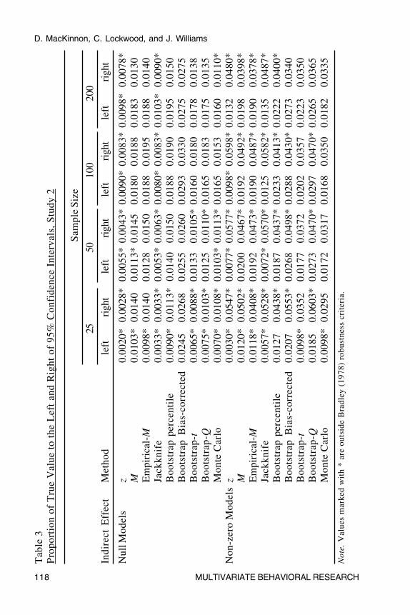
Results

Confidence Limits

Table 3 shows the proportion of times the true indirect effect was greaterthan or less than the confidence interval generated by each method for 95%confidence limits. In the interest of conserving space, we present the resultsonly for the 95% confidence interval averaged across parameter values. Theresults for each parameter combination and for 90% and 80% confidenceintervals are comparable and are available from the first author. The samepattern of results for the M and z confidence limits observed in Study 1 wereobtained in Study 2. The M confidence limits are closer to the expectedpercentages than the confidence limits based on the normal distribution. Formodels where the true indirect effect equals 0, the percentages are almostalways lower than .025, suggesting that the sample confidence intervals are toowide. Only the bias-corrected bootstrap has some percentages that are largerthan the robustness interval, and this occurred most often for the � = 0 � = .39and � = 0 � =.59 parameter combinations. Averaging across parameter valueconditions for a true indirect effect equal to 0, only the bias-corrected bootstrapis never outside the robustness intervals. All other approaches tend to havepercentages that are too small. Overall, percentages are more likely to beinside the robustness interval as effect size and sample size increase.

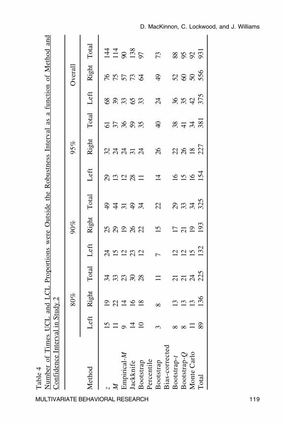
Table 4 summarizes the performance of the confidence limits by showingthe number of times that the observed percentage was outside the robustnessinterval for each of the three confidence intervals and nine methods3. Asshown in Table 4 for the 95% confidence interval, the observed percentagewas outside the robustness interval 34-41 times for the two distribution of the

3 Two resampling methods were investigated but are not reported in the text to conservespace and because the results were similar to methods in the article. The accelerated biascorrection bootstrap method was also applied with the results comparable to but not betterthan the bias-corrected bootstrap. A method we labeled the Q-transform was alsoinvestigated in this research. The method consists of applying the transformation inEquation 9 but not transforming the Q back to a T using Equation 10. In general thismethod had somewhat better performance than the Bootstrap-Q although not as good asthe bias corrected bootstrap.



product tests and all resampling methods except the jackknife. All of thesemethods were considerably better than the jackknife (59 times) which onlyhad slightly better performance than the traditional z test (61 times). Lookingat the totals across all three confidence intervals, the bias-correctedbootstrap had the best performance with 73 times outside the robustnessinterval. The Empirical-M (90), bootstrap percentile (97), bootstrap-t (88),bootstrap-Q (95) and Monte Carlo (92) all had generally similarperformance. The M test (114) appears to be intermediate between thesemore accurate methods and the traditional z (144) and jackknife (138) whichhad the worst performance overall. Although not shown in the tables, thesame pattern of results were also observed for squared bias (observed TypeI error rate minus expected Type I error rate squared).

The Type I error rates and observed power of the single sample andresampling methods are shown in Table 5 for the .05 level of statisticalsignificance. As in Table 3, the Type I error rates are always smaller thanpredicted for each method with the exception of the bias-corrected bootstrapwhich is also the only method that on average has rates that are not outsidethe robustness interval. With the exception of the traditional z and thejackknife, all tests have Type I error rates that are not outside the robustnessinterval for sample size of at least 100. The bias-corrected method also hadthe most statistical power overall, followed by the bootstrap-Q, M, andEmpirical-M, which had very similar overall power values. The percentilebootstrap, Monte Carlo, and bootstrap-t test had very similar overall power.The traditional z test and jackknife were similar and had considerably lesspower than the other methods.

Discussion

The different tests can be grouped in four general categories based onthe results of Study 2. The confidence limits based on the jackknife and thetraditional z test are in the first group of tests which had the worstperformance of all the tests with the least power and the lowest Type I errorrates. The second group of tests consists of the percentile bootstrap,bootstrap-t and Monte Carlo tests which have comparable power andconfidence limits that tend to be too wide. The third group of tests, M test,Empirical-M test, and the bootstrap-Q, have more power and confidencelimits that are not as wide as the tests in the second group. All of these testshad Type I errors that were never above the robustness interval, yet hadmore power than the methods in the first two groups. If a researcher wantedto avoid exceeding nominal Type I error rates, these are the methods ofchoice. The fourth group consists of the bias-corrected bootstrap which had



Tab

le 3

Pro

port

ion

of T

rue

Val

ue t

o th

e L

eft

and

Rig

ht o

f 95

% C

onfi

denc

e In

terv

als,

Stu

dy 2

Sam

ple

Siz

e

2550

100

200

Indi

rect

Eff

ect

Met

hod

left

righ

tle

ftri

ght

left

righ

tle

ftri

ght

Nul

l Mod

els

z0.

0020

*0.

0028

*0.

0055

*0.

0043

*0.

0090

*0.

0083

*0.

0098

*0.

0078

*M

0.01

03*

0.01

400.

0113

*0.

0145

0.01

800.

0188

0.01

830.

0130

Em

piri

cal-

M0.

0098

*0.

0140

0.01

280.

0150

0.01

880.

0195

0.01

880.

0140

Jack

knif

e0.

0033

*0.

0033

*0.

0053

*0.

0063

*0.

0080

*0.

0083

*0.

0103

*0.

0090

*B

oots

trap

per

cent

ile

0.00

90*

0.01

13*

0.01

400.

0150

0.01

880.

0190

0.01

950.

0150

Boo

tstr

ap B

ias-

corr

ecte

d0.

0245

0.02

680.

0255

0.02

600.

0293

0.03

300.

0275

0.02

75B

oots

trap

-t0.

0065

*0.

0088

*0.

0133

0.01

05*

0.01

600.

0180

0.01

780.

0138

Boo

tstr

ap-Q

0.00

75*

0.01

03*

0.01

250.

0110

*0.

0165

0.01

830.

0175

0.01

35M

onte

Car

lo0.

0070

*0.

0108

*0.

0103

*0.

0113

*0.

0165

0.01

530.

0160

0.01

10*

Non

-zer

o M

odel

sz

0.00

30*

0.05

47*

0.00

77*

0.05

77*

0.00

98*

0.05

98*

0.01

320.

0480

*M

0.01

20*

0.05

02*

0.02

000.

0467

*0.

0192

0.04

92*

0.01

980.

0398

*E

mpi

rica

l-M

0.01

18*

0.04

08*

0.01

920.

0473

*0.

0190

0.04

87*

0.01

900.

0378

*Ja

ckkn

ife

0.00

57*

0.05

28*

0.00

72*

0.05

70*

0.01

250.

0582

*0.

0135

0.04

87*

Boo

tstr

ap p

erce

ntil

e0.

0127

0.04

38*

0.01

870.

0437

*0.

0233

0.04

13*

0.02

220.

0400

*B

oots

trap

Bia

s-co

rrec

ted

0.02

070.

0553

*0.

0268

0.04

98*

0.02

880.

0430

*0.

0273

0.03

40B

oots

trap

-t0.

0098

*0.

0352

0.01

770.

0372

0.02

020.

0357

0.02

230.

0350

Boo

tstr

ap-Q

0.01

850.

0603

*0.

0273

0.04

70*

0.02

970.

0470

*0.

0265

0.03

65M

onte

Car

lo0.

0098

*0.

0295

0.01

720.

0317

0.01

680.

0350

0.01

820.

0335

Not

e. V

alue

s m

arke

d w

ith

* ar

e ou

tsid

e B

radl

ey (

1978

) ro

bust

ness

cri

teri

a.



Tab

le 4

Num

ber

of T

imes

UC

L a

nd L

CL

Pro

port

ions

wer

e O

utsi

de t

he R

obus

tnes

s In

terv

al a

s a

func

tion

of

Met

hod

and

Con

fide

nce

Inte

rval

in S

tudy

2 80%

90%

95%

Ove

rall

Met

hod

Lef

tR

ight

Tot

alL

eft

Rig

htT

otal

Lef

tR

ight

Tot

alL

eft

Rig

htT

otal

z15

1934

2425

4929

3261

6876

144

M11

2233

1529

4413

2437

3975

114

Em

piri

cal-

M9

1423

1219

3112

2436

3357

90Ja

ckkn

ife

1416

3023

2649

2831

5965

7313

8B

oots

trap

1018

2812

2234

1124

3533

6497

Per

cent

ile

Boo

tstr

ap3

811

715

2214

2640

2449

73B

ias-

corr

ecte

dB

oots

trap

-t8

1321

1217

2916

2238

3652

88B

oots

trap

-Q8

1321

1221

3315

2641

3560

95M

onte

Car

lo11

1324

1519

3416

1834

4250

92T

otal

8913

622

513

219

332

515

422

738

137

555

693

1



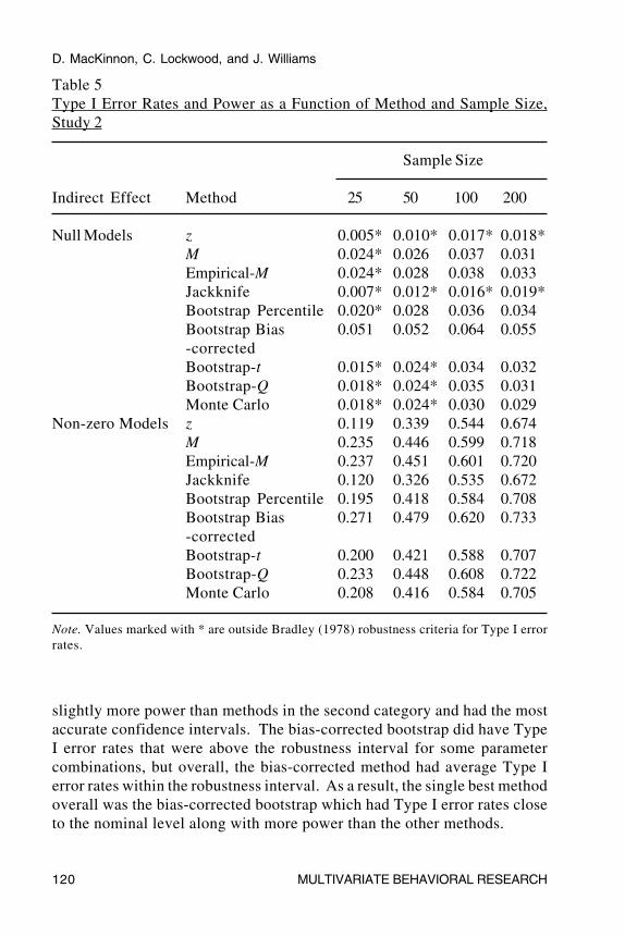
slightly more power than methods in the second category and had the mostaccurate confidence intervals. The bias-corrected bootstrap did have TypeI error rates that were above the robustness interval for some parametercombinations, but overall, the bias-corrected method had average Type Ierror rates within the robustness interval. As a result, the single best methodoverall was the bias-corrected bootstrap which had Type I error rates closeto the nominal level along with more power than the other methods.

Table 5Type I Error Rates and Power as a Function of Method and Sample Size,Study 2

Sample Size

Indirect Effect Method 25 50 100 200

Null Models z 0.005* 0.010* 0.017* 0.018*M 0.024* 0.026 0.037 0.031Empirical-M 0.024* 0.028 0.038 0.033Jackknife 0.007* 0.012* 0.016* 0.019*Bootstrap Percentile 0.020* 0.028 0.036 0.034Bootstrap Bias 0.051 0.052 0.064 0.055-correctedBootstrap-t 0.015* 0.024* 0.034 0.032Bootstrap-Q 0.018* 0.024* 0.035 0.031Monte Carlo 0.018* 0.024* 0.030 0.029

Non-zero Models z 0.119 0.339 0.544 0.674M 0.235 0.446 0.599 0.718Empirical-M 0.237 0.451 0.601 0.720Jackknife 0.120 0.326 0.535 0.672Bootstrap Percentile 0.195 0.418 0.584 0.708Bootstrap Bias 0.271 0.479 0.620 0.733-correctedBootstrap-t 0.200 0.421 0.588 0.707Bootstrap-Q 0.233 0.448 0.608 0.722Monte Carlo 0.208 0.416 0.584 0.705

Note. Values marked with * are outside Bradley (1978) robustness criteria for Type I errorrates.



Example

The following example illustrates the methods used in this article withdata from the Adolescents Training and Learning to Avoid Steroids(ATLAS) program. The ATLAS program is a multi-component programadministered to high school football players to prevent use of anabolicandrogenic steroids (AAS). More details of the program may be found inGoldberg et al. (1996) and single and multiple mediator model results usingthe standard z significance test for the mediated effect may be found inMacKinnon et al. (2001). The data for this simplified example were from 861cases (from 15 treatment schools and 16 control schools) with complete dataon three variables, X-exposure to the program or not, X

M-perceived severity

of anabolic steroid use, and Y-nutrition behaviors. One part of the programwas designed to increase the perceived severity of using steroids, which washypothesized to increase proper nutrition behaviors.

Confidence limits for the indirect effect were computed for three singlesample tests: the traditional z, the M test, and the empirical-M test, as wellas six resampling methods: the jackknife, percentile bootstrap, bootstrap-t,bootstrap-Q, bias-corrected bootstrap, and the Monte Carlo method.Ninety-five percent confidence limits were formed for the data using eachmethod as described in Study 2. For the jackknife, 861 samples were drawnfrom the original data, each one excluding a different case. All bootstrapmethods were performed with 1000 resamples from the original data.Additionally, 1000 Monte Carlo samples were generated using the observedestimates of �, �, �

�, and �

� (.2731, .0736, .0894, and .0300 respectively).

The indirect effect equaled .0201 with a standard error of .0105 usingEquation 4. These values were used with Equation 5 to find upper and lowerconfidence limits for the z method. The M test limits were found using thesample values of �

� = 3.0539 and �

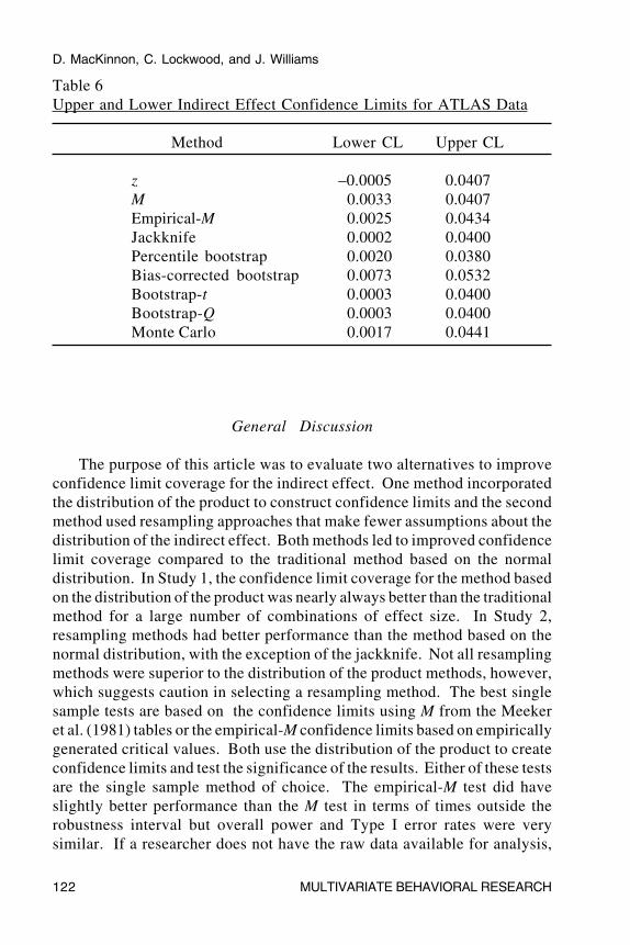
� = 2.4486. Critical values were thenfound in the augmented Meeker et al. (1981) tables using rounded values of3 and 2.4. The upper critical M value was 2.2683 and the lower was equalto –1.5969. These values were used in Equations 6 and 7 to find the upperand lower M test confidence limits. Table 6 presents the upper and lowerconfidence limits of the mediated effect using these single sample methodsand the resampling tests. The results demonstrate many of the findings ofthe simulation studies. First, zero is included in the confidence limits for thetraditional z method, which would lead to the conclusion that the indirecteffect is nonsignificant. When the more powerful M test is used however,the effect is statistically significant. The resampling approaches also suggesta significant indirect effect.



Table 6Upper and Lower Indirect Effect Confidence Limits for ATLAS Data

Method Lower CL Upper CL

z –0.0005 0.0407M 0.0033 0.0407Empirical-M 0.0025 0.0434Jackknife 0.0002 0.0400Percentile bootstrap 0.0020 0.0380Bias-corrected bootstrap 0.0073 0.0532Bootstrap-t 0.0003 0.0400Bootstrap-Q 0.0003 0.0400Monte Carlo 0.0017 0.0441

General Discussion

The purpose of this article was to evaluate two alternatives to improveconfidence limit coverage for the indirect effect. One method incorporatedthe distribution of the product to construct confidence limits and the secondmethod used resampling approaches that make fewer assumptions about thedistribution of the indirect effect. Both methods led to improved confidencelimit coverage compared to the traditional method based on the normaldistribution. In Study 1, the confidence limit coverage for the method basedon the distribution of the product was nearly always better than the traditionalmethod for a large number of combinations of effect size. In Study 2,resampling methods had better performance than the method based on thenormal distribution, with the exception of the jackknife. Not all resamplingmethods were superior to the distribution of the product methods, however,which suggests caution in selecting a resampling method. The best singlesample tests are based on the confidence limits using M from the Meekeret al. (1981) tables or the empirical-M confidence limits based on empiricallygenerated critical values. Both use the distribution of the product to createconfidence limits and test the significance of the results. Either of these testsare the single sample method of choice. The empirical-M test did haveslightly better performance than the M test in terms of times outside therobustness interval but overall power and Type I error rates were verysimilar. If a researcher does not have the raw data available for analysis,



resampling methods described in this article cannot be conducted and thesesingle sample methods are the only methods available.

The bias-corrected bootstrap is the method of choice if resamplingmethods are feasible. There are limitations to the use of resampling methods,however. These include the lack of statistical software to conduct theanalysis and the increased computational time required for the analysis. Thebias-corrected bootstrap is included as an option in the AMOS (Arbuckle &Wothke, 1999) covariance structure analysis program. The EQS programand LISREL programs can be used to conduct resampling analyses but theuser must write a separate program to compute the bootstrap method afterthese programs write out the results of each individual bootstrap sample. Allof the resampling tests used in this article are now included in an updatedversion of the SAS program in Lockwood and MacKinnon (1998).Computation time does not seem like a reasonable argument for not usingresampling methods because of the speed of current computing, althoughrelatively large models may take considerable time.

Another potential limitation of resampling methods is that the differencebetween resampling methods and single sample methods is small in manycases. In fact, Bollen and Stine (1990) report percentile bootstrapconfidence limits and not bias-corrected bootstrap confidence limits becausetheir limits were so similar. In the present study for example, the biascorrected bootstrap and the z test came to the different conclusionsregarding whether the population value was inside or outside the confidenceinterval only 5.5% of the time across all confidence intervals examined in thisstudy. The discrepancy between the bias-corrected bootstrap and the M testwas only 4.5%. As shown in the example data, the confidence limits werevery similar across the methods, although only the traditional z included zeroin the confidence interval. There is some evidence from this study that forcases where the values of either �

� and

�

� are large, resampling methods do

not provide much improvement over single sample methods. The additionaleffort required for resampling methods may not be justified in these cases.When confidence limits are required for rather small values of �

� and

�

�, then

the resampling methods are more accurate than single sample tests. A finallimitation of resampling tests has been called the first law of statisticalanalysis (Gleser, 1996). The law requires that any two statisticians analyzingthe same data set with the same methods should come to identicalconclusions. With resampling methods (other than the jackknife), it ispossible that different conclusions could be reached because the resampleddata sets generated by different statisticians will differ.

The results of this study highlight a difference between testing significancebased on critical values versus confidence limits. There is a problematic result



of testing the significance of the indirect effect with the distribution of the productusing the critical value for the distribution for � = 0 and � = 0, which is 2.18 fora .05 Type I error rate. In this situation, either � or � can be nonsignificant butthe test based on the distribution of the product may be significant, indicating thatthe indirect effect is larger than expected by chance alone while one of theregression coefficients contributing to its effect is not. The statistical test ofwhether � = 0 and � = 0 is more likely to be judged significant when the truevalues are � = 0 and � 0 or � 0 and � = 0, because the distribution ofthe indirect effect with these parameter values differs from the distributionfor � = � = 0. By selecting the critical value of 2.18 from the distribution of theproduct for � = 0 and � = 0, the null hypothesis is H

0: � = 0 and � = 0, which is

rejected in three situations: when � 0 and � 0, � = 0 and � 0, or � 0and � = 0. The traditional z test is a test of the null hypothesis H

0: �� = 0, which

is rejected only when � 0 and � 0 but the assumption of the z distributiondoes not appear to be accurate for the product of � and �, altering the Type Ierror rates and statistical power of this test. The M test of significance basedon confidence limits also tests whether �� = 0 and requires different criticalvalues for the upper and lower limits. In this case a test of H

0: � = 0 and � = 0

yields a different result than the test based on confidence limits.There are other methods to evaluate indirect effects. These include the

steps mentioned in Baron and Kenny (1986) and Judd and Kenny (1981) andthe joint significance test of � and � described in MacKinnon et al. (2002),which do not include explicit methods to compute confidence limits. Thereare other methods to compute confidence limits for the indirect effect basedon the standard error of the difference in coefficients, � – �� (e.g., Allison,1995b ; Clogg, Petkova, & Cheng, 1995; Clogg, Petkova, & Shihadeh, 1992;Olkin & Finn, 1995) but these methods perform similar to the traditional z testdescribed in this article, in part because a normal distribution for the indirecteffect is assumed.

There are several limitations of this article. The results may not extendbeyond the single indirect effect model investigated. The influence ofdifferent distributions of X, X

M, and Y

O was not evaluated. However, Study

1 included a binary independent variable as another condition. Because theresults were virtually identical to the results for a continuous independentvariable, they were not reported in this article. Use of the M test confidencelimits for indirect effects consisting of the product of three or more pathswould require the use of the distribution of the product of three or morerandom variables. There are analytical solutions for this distribution(Springer, 1979) but tabled values of the distribution are not available. Theresampling methods can be applied to these more complicated models.



This article has also been silent regarding important conceptual issues ininterpreting indirect effects. Here it is assumed that the indirect effect modelis known and that X precedes X

M and X

M precedes Y

O. In practice, the

hypothesized chain of effects in an indirect effect may be wrong and theremay be several equivalent models that will explain the relations equally well.For example, the mediating variable may actually change the independentvariable that may then affect the dependent variable. In the case of arandomized experiment, the independent variable improves interpretationbecause it must precede the mediating variable and the dependent variable,but even in this situation the interpretation of indirect effects is morecomplicated than what might be expected (Holland, 1988; Sobel, 1998).Issues regarding the specificity of the effect to one or a few of manymediating variables and future experiments targeted at specific mediatingvariables improve the veracity of indirect effects (West & Aiken, 1997).None of these methods to test the statistical significance or computeconfidence limits for indirect effects answer these critical conceptualquestions, but when combined with careful replication studies these relationsare clarified.

There are several ways that the confidence limits described in this articlemay be further improved. One approach is to use more extensive resamplingmethods such as bootstrapping residuals, iterated bootstrap, or methods tocompute confidence limits based on the permutation test (Manly, 1997).More extensive tables for the M test critical values may also improve theperformance of this method. Analytical work on the distribution of theproduct of two regression coefficients especially for small sample sizes mayalso lead to more accurate confidence limits.

The practical implication of the results of this article is that the traditionalz test confidence limits can be substantially improved by using a method suchas the M test that incorporates the distribution of the product of two normalrandom variables. The bias-corrected bootstrap provided the most accurateconfidence limits and greatest statistical power, and is the method of choiceif it is feasible to conduct resampling methods.

References

Ajzen, I. & Fishbein, M. (1980). Understanding attitudes and predicting social behavior.Englewood Cliffs, NJ: Prentice Hall.

Allison, P. D. (1995a). Exact variance of indirect effects in recursive linear models.Sociological Methodology, 25, 253-266.

Allison, P. D. (1995b). The impact of random predictors on comparisons of coefficientsbetween models: Comment on Clogg, Petkova, and Haritou. American Journal ofSociology, 100, 1294-1305.



Alwin, D. F. & Hauser, R. M. (1975). The decomposition of effects in path analysis.American Sociological Review, 40, 37-47.

Arbuckle, J. L. & Wothke, W. (1999). Amos 4.0 users’ guide version 3.6. Chicago:Smallwaters.

Aroian, L. A. (1947). The probability function of the product of two normally distributedvariables. Annals of Mathematical Statistics,18, 265-271.

Aroian, L. A., Taneja, V. S., & Cornwell, L. W. (1978). Mathematical forms of thedistribution of the product of two normal variables. Communications in Statistics:Theory and Methods, A7, 165-172.

Bandura, A. (1977). Social learning theory. Englewood Cliffs, NJ: Prentice-Hall.Baron, R. M. & Kenny, D. A. (1986). The moderator-mediator variable distinction in

social psychological research: Conceptual, strategic, and statistical considerations.Journal of Personality and Social Psychology, 51, 1173-1182.

Bentler, P. M. (1997). EQS for Windows (Version 5.6) [Computer program]. Encino, CA:Multivariate Software, Inc.

Bollen, K. A. & Stine, R. (1990). Direct and indirect effects: Classical and bootstrapestimates of variability. Sociological Methodology, 20, 115-140.

Bradley, J. V. (1978). Robustness? British Journal of Mathematical and StatisticalPsychology, 31, 144-152.

Chernick, M. R. (1999). Bootstrap methods: A practitioner’s guide. New York: Wiley.Clogg, C. C., Petkova, E., & Cheng, T. (1995). Reply to Allison: More on comparing

regression coefficients. American Journal of Sociology, 100, 1305-1312.Clogg, C. C., Petkova, E., & Shihadeh, E. S. (1992). Statistical methods for analyzing

collapsibility in regression models. Journal of Educational Statistics, 17, 51-74.Cohen, J. (1988). Statistical power analysis for the behavioral sciences. Hillsdale, NJ:

Lawrence Erlbaum Associates.Craig, C. C. (1936). On the frequency function of xy. Annals of Mathematical Statistics, 7,

1-15.Duncan, O. D., Featherman, D. L., & Duncan, B. (1972). Socioeconomic background and

achievement. New York: Seminar Press.Efron, B. & Tibshirani, R. J. (1993). An introduction to the bootstrap. New York:

Chapman & Hall.Gleser, L. J. (1996). Comment on “Bootstrap Confidence Intervals” by T. J. DiCiccio and

B. Efron. Statistical Science, 11, 219-221.Goldberg, L., Elliot, D., Clarke, G. N., MacKinnon, D. P., Moe, E., Zoref, L., et al. (1996).

Effects of a multi-dimensional anabolic steroid prevention intervention: TheAdolescents Training and Learning to Avoid Steroids (ATLAS) program. Journal ofthe American Medical Association, 276, 1555-1562.

Hansen, W. B. & Graham, J. W. (1991). Preventing alcohol, marijuana, and cigarette useamong adolescents: Peer pressure resistance training versus establishing conservativenorms. Preventive Medicine, 20, 414-430.

Hanushek, E. A. & Jackson, J. E. (1977). Statistical methods for social scientists. NewYork: Academic Press.

Harlow, L. L., Mulaik, S. A., & Steiger, J. H. (Eds.). (1997). What if there were nosignificance tests? Mahwah, NJ: Erlbaum.

Hawkins, J. D., Catalano, R. F. & Miller, J. Y. (1992). Risk and protective factors foralcohol and other drug problems in adolescence and early adulthood: Implications forsubstance abuse prevention. Psychological Bulletin, 112, 64-105.

Holland, P. W. (1988). Causal inference, path analysis, and recursive structural equationmodels. Sociological Methodology, 18, 449-484.



Hoyle, R. H. & Kenny, D. A. (1999). Sample size, reliability, and tests of statisticalmediation. In R. H. Hoyle (Ed.), Statistical strategies for small sample research (pp.195-222). Thousand Oaks, CA: Sage.

Hyman, H. H. (1955). Survey design and analysis: Principles, cases and procedures.Glencoe: The Free Press.

James, L. R. & Brett, J. M. (1984). Mediators, moderators, and tests for mediation.Journal of Applied Psychology, 69, 307-321.

Jöreskog, K. G. & Sörbom, D. (1993). LISREL (Version 8.12) [Computer program].Chicago: Scientific Software International.

Judd, C. M. & Kenny, D. A. (1981). Process analysis: Estimating mediation in treatmentevaluations. Evaluation Review, 5, 602-619.

Krantz, D. H. (1999). The null hypothesis testing controversy in psychology. Journal ofthe American Statistical Association, 94, 1372-1381.

Lockwood, C. M. & MacKinnon, D. P. (1998). Bootstrapping the standard error of themediated effect. In Proceedings of the Twenty-third Annual SAS Users GroupInternational Conference (pp. 997-1002). Cary, NC: SAS Institute.

Lomnicki, Z. A. (1967). On the distribution of products of random variables. Journal ofthe Royal Statistical Society, 29, 513-524.

MacKinnon, D. P. (1994). Analysis of mediating variables in prevention and interventionresearch. National Institute on Drug Abuse Research Monograph Series, 139, 127-153.

MacKinnon, D. P. & Dwyer, J. H. (1993). Estimating mediated effects in preventionstudies. Evaluation Review, 17, 144-158.

MacKinnon, D. P., Goldberg, L., Clarke, G. N., Elliot, D. L., Cheong, J., Lapin, A., et al.(2001). Mediating mechanisms in a program to reduce intentions to use anabolicsteroids and improve exercise self-efficacy and dietary behavior. Prevention Science,2, 15-28.

MacKinnon, D. P., Johnson, C. A., Pentz, M. A., Dwyer, J. H., Hansen, W. B., Flay, B. R.& Wang, E. Y. I. (1991). Mediating mechanisms in a school-based drug preventionprogram: First year effects of the Midwestern Prevention Project. Health Psychology,10, 164-172.

MacKinnon, D. P., Lockwood C. M., Hoffman, J. M., West, S. G., & Sheets, V. (2002). Acomparison of methods to test the significance of mediation and other interveningvariable effects. Psychological Methods, 7, 83-104.

MacKinnon, D. P., Warsi, G., & Dwyer, J. H. (1995). A simulation study of mediatedeffect measures. Multivariate Behavioral Research, 30, 41-62.

Manly, B. F. (1997). Randomization and Monte Carlo methods in biology. New York:Chapman and Hall.

McDonald, R. P. (1997). Haldane’s lungs: A case study in path analysis. MultivariateBehavioral Research, 32, 1-38.

Meeker, W. Q., Jr., Cornwell, L. W., & Aroian, L. A. (1981). Selected tables inmathematical statistics, volume VII: The product of two normally distributed randomvariables. Providence, RI: American Mathematical Society.

Meeker, W. Q., Jr., & Escobar, L. A. (1994). An algorithm to compute the cdf of theproduct of two normal random variables. Communications in Statistics: Simulationand Computation, 23, 271-280.

Mosteller, F. & Tukey, J. W. (1977). Data analysis and regression: A second course instatistics. Reading, MA: Addison-Wesley.

Noreen, E. W. (1989). Computer-intensive methods for testing hypotheses: An introduction.New York: John Wiley & Sons.



Olkin, I. & Finn, J. D. (1995). Correlations redux. Psychological Bulletin, 118, 155-164.Rodgers, J. L. (1999). The bootstrap, the jackknife, and the randomization test: A

sampling taxonomy. Multivariate Behavioral Research, 34, 441-456.SAS Institute. (1989). SAS (Version 6.12) [Computer program]. Cary, NC: Author.Schoenberg, R. & Arminger, G. (1996). LINCS (Version 2.0) [Computer program]. Maple

Valley, WA: Aptech Systems, Inc.Shrout, P. E. & Bolger, N. (2002). Mediation in experimental and nonexperimental studies:

New procedures and recommendations. Psychological Methods, 7, 422-445.Sobel, M. E. (1982). Asymptotic confidence intervals for indirect effects in structural

equation models. Sociological Methodology, 13, 290-312.Sobel, M. E. (1986). Some new results on indirect effects and their standard errors in

covariance structure models. Sociological Methodology, 16, 159-186.Sobel, M. E. (1987). Direct and indirect effects in linear structural equation models.

Sociological Methods & Research, 16, 155-176.Sobel, M. E. (1990). Effect analysis and causation in linear structural equation models.

Psychometrika, 55, 495-515.Sobel, M. E. (1998). Causal inference in statistical models of the process of socioeconomic

achievement: A case study. Sociological Methods and Research, 27, 318-348.Springer, M. D. (1979). The algebra of random variables. New York: John Wiley and Sons.Springer, M. D. & Thompson, W. E. (1966). The distribution of independent random

variables. SIAM Journal on Applied Mathematics, 14, 511-526.Stone, C. A. & Sobel, M. E. (1990). The robustness of estimates of total indirect effects in

covariance structure models estimated by maximum likelihood. Psychometrika, 55,337-352.

Tobler, N. S. (1986). Meta-analysis of 143 adolescent drug prevention programs:Quantitative outcome results of program participants compared to a control orcomparison group. Journal of Drug Issues, Fall, 537-567.

Turner, R. J., Wheaton, B., & Lloyd, D. A. (1995). The epidemiology of social stress.American Sociological Review, 60, 104-125.

Warner, B. D. & Rountree, P. W. (1997). Local social ties in a community and crimemodel: Questioning the systemic nature of informal social control. Social Problems,44, 520-536.

West, S. G. & Aiken, L. S. (1997). Towards understanding individual effects in multiplecomponent prevention programs: Design and analysis strategies. In K. Bryant, M.Windle, & S. West (Eds.), The science of prevention: Methodological advances fromalcohol and substance abuse research (pp. 167-209). Washington, DC: AmericanPsychological Association.

Wolchik, S. A., Ruehlman, L. S., Braver, S. L., & Sandler, I. N. (1989). Social support ofchildren of divorce: Direct and stress buffering effects. American Journal ofCommunity Psychology, 17, 485-501.

Accepted June, 2003.

confidence limits for the indirect effect: distribution of

Documents