lntroducing Confidence Bounds and Confidence Levels into lterated

Fractional Factorial Design Analysis

Wayne Hajas A Practicum Submitteâ to the Faculty of Graduate Studies in

Partial Fulfillment of the Requirements for the Degree of

Master of Mathematical and Corn putational Sciences lnstitute of lnd ustrial Mathematics

University of Manitoba Winnipeg, Manitoba

Nationai Library Bibliothèque nationale du Canada

Acquisitions and Acquisitions et BibliographicServices servicesbibliographiques

395 Wellington Street 395. rue Wellington OtoiwaON K I A W OttawaON K 1 A M canada canada

The author has granted a non- L'auteur a accordé une licence non exclusive licence allowing the exclusive permettant à la National Library of Canada to Bibliothèque nationale du Canada de reproduce, loan, distriiute or seU reproduire, prêter, distribuer ou copies of this thesis in microfixm, vendre des copies de cette thèse sous paper or electronic formais. la forme de microfiche/nlm, de

reproduction sur papier ou sur format élecîronique.

The author retains ownership of the L'auteur conserve la propriété du copyright in this thesis. Neither the droit d'auteur qui protège cette thèse. thesis nor substantial extracts fkom it Ni la thèse ni des extraits substantiels may be printed or otherwise de celle-ci ne doivent être imprimés reproduced without the author's ou autrement reproduits sans son permission. autorisation.

THE LW'ERSITk' OF 5LWITOBX

F.4CcLTY OF GRmt'ATE STUDIES *****

COPYRIGHT PERWSSION PAGE

A ThesislPracticurn submitted to the Faculty of Graduate Studies of The University

of Manitoba in parlia1 fulfitlment of the requirements of the degree

of

W T E R OF SCIENCE

Permission has been granted to the Library of The University of Manitoba to lend o r sell copies of this thesis/practicum, to the National Library of Canada to microfilm this thesis

and to lend or sel1 copies of the film, and to Dissertations Abstracts International to publish an abstract of this thesis/practicum.

The author resemes other publication riphts, and neither this thesislpracticum nor extensive extracts frorn it may be printed or othenvise reproduced without the author's

written permission.

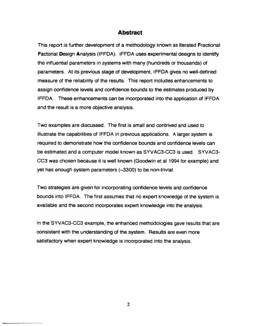
Abstract

This report is further developrnent of a methodology known as lterated Fractional

Factorial Design Analysis (IFFDA). IFFDA uses experimental designs to identify

the influential parameters in systems with many (hundreds or thousands) of

parameters. At its previous stage of developrnent, IFFDA gives no welldefined

measure of the reliability of the results. This report includes enhancements to

assign confidenœ levels and confidenœ bounds to the estimates produœd by

IFFDA. These enhancements can be incorporated into the application of IFFDA

and the result is a more objective analysis.

Two examples are discussed. The first is smail and contrived and used to

illustrate the capabilities of 1 FFDA in previous applications. A larger system is

required to demonstrate how the confidence bounds and confidenœ levels c m

be estimated and a computer mode1 known as SYVAC3-CC3 is used. SYVAC3-

CC3 was chosen because it is well known (Goodwin et al 1994 for example) and

yet has enough systern parameters (-3300) to be non-trivial.

Two strategies are given for incorporating confidence levels and confidence

bounds into IFFDA. The first assumes that no expert knowledge of the system is

available and the second incorporates expert knowledge into the analysis.

In the SYVAC3-CC3 example, the enhanced methodologies gave results that are

consistent with the understanding of the system. Results are even more

satisfactory when expert knowledge is incorporated into the analysis.

Acknowiedgements

I would like to thank my supeMsing cornmittee for Meir help in developing and

documenting the meoiods presented in this report; Terry Andres of AECL and

Lynn Batten, Lai Chan. and Ken Mount of the University of Manitoba.

Abstract

Acknowledgernents

Table Of Contents

List Of Tables

List Of Figures

1 . Introduction And Summary

1.1. Motivation For IFFDA

1.2. History Of IFF DA

1 -3. A Brief Explanation Of The Methodology

1 -3.1 . The Design

1 -3.2. Estimating Main Effects And Interactions

1.3.3. Confidence Coefficients and Confidence Bounds For

The Estimated Main Effects And Interactions

1.3.4. Refining The Estimated Values Of Main Effects

And Interactions

1.3.5. Estimating Quadratic Effects

1.3.6. Confidence Coefficients and Confidence Bounds For

The Estimated Quadratic Effects

1 -3.7. Refining The Estimated Values Of Quadratic Effects

1.4. Examples To Be Discussed

1 -4.1. Small Example

1.4.2. SYVAC3-CC3 Example

2. Experimental Designs In The Example Applications

2.1 . Small Example

2.2. SYVAC3-CC3 Exarnple

3. Estimating Effects In The Small Exarnple

3.1 . Estimating Main Eff ects And Interactions

3.2. Estimated Quadratic Effects

3.3. Refining Estimates Of Main Effects And Interacüons

3.4. Refining Estimates Of Qwdratic Effects

4. Confidence Levels And Confidence Bounds In The SYVAC3-CC3

Example

4.1 . The Estimated Effects

4.2. Main Effects And Interactions

4.3. Quadratic Effects

5. Applying The Cahulations To A Large System

5.1 . A Purety Statistical Basis

5.2. lncorporating Expert Knowledge Of A System

6. Conclusions

7. Recomrnendations

7.1. lnvestigate Variations On The Experïmental

Designs To Optimize Results

7.2. Incorporate Better Statistical Methods To Estirnate

The Confidence Coefficients And Confidence Bounds

7.3. lnvestigate Using ANOVA To Analyze Main Effects And

l nteractions

7.4. lnvestigate The Influence Of Aliased System Parameters On The

Estimated Quadratic Effects 69

7.5. Incorporate The Analysis Stage Of IFFDA lnto A

Formal Software Package 69

Bibliography 70

Appendix : Glossary Of Terms And Symbols 71

List Of Tables

1.4.2.1 Some SYVAC3-CC3 Parameters Discussed In This Report 18

2.1.1 Assignment Of System Parameters To Experimental

Factors For The Srnall Example 20

2.1 -2 Experirnental Factors, Systern Parameters and System

Responses for the Small Example 23

2.1 -3 Estimable Effects For The Small Example. Initial

Estimates.

Assignment Of Some SYVAC3-CC3 Parameters To

Experimental Factors. 27

The Estimation Of Main Effects And Interactions For

The Small Example. 30

System Effects As Estimated By The Streamlined

3.1 -2 System Eff ects As Estimated By The Streamlined

Approach For The Small Example. Original Estimates.

3.2.1 lteration Averages For The Small Example.

3.2.2: Estimated Quadratic Effects For The Small Example.

Original Estimates.

3.3.1 Estimated Main Effects And Interactions For The Srnall

Example After One Refinement Of The Results.

Estimated Main Effects And Interactions For The Small

Example After Two Refinements Of The Results. 36

lteration Averages For The Small Example After One

Refinement. 37

3.4.2 Estirnated Quadratic Effects For The Small Example After One

Refinernent. 37

4.1 -1 The Largest Estimated Main Effects For SWAC3-CC3.

Original Estimates. 40

4.1 -2 The Largest Estimated Quadratic Effects For SYVAC3-CC3.

Original Estimates. 41

The iargest Estimated Main Effects For SYVAC3-CC3

After One Revision.

4.2.2 The Largest Estimated Main Effects For SYVAC3-CC3

After Three Revisions. 49

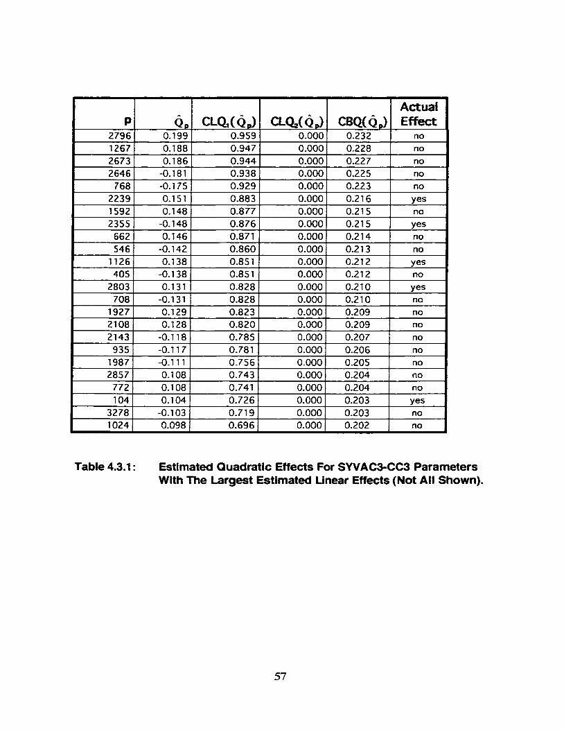
4.3.1 Estimated Quadratic Effects For SYVAC3-CC3 Parameters With

The Largest Estimated Main Linear Effects (Not All Shown).

Results Of IFFDA If No Expert Knowledge Of ÇYVAC3-CC3

Is Availabte.

Results Of IFFDA When Expert Knowledge Of SYVAC3-CC3

Is Available.

List Of Figures

1.3.5.1 l t 1 ustration Of A Quadratic Effect 15

4.2.1 Distribution Of Estimable Effects 43

4.2.2 Distribution Of Estimated Main System Effects 44

4.3.1 Distribution Of Average Responses From lterations Of The

Sub-Design 55

4.3.2 Distribution Of Estimated Quadratic Effects 56

Chapter 1

Introduction and Summary

1.1 Motivation for IFFDA

lterated Fractional Factorial Design Analysis (IFFDA) was developeâ for

sensitivity analysis of a family of cornputer models associated with SYstems

Variable Analysis Code (SYVAC) (Goodwin et al. 1 994 and Goodwin et al. 1 996).

These rnodels are used to predict the impact of nuclear waste repositories.

Sensitivity analysis of these models is challenging because:

There are many (hundreds or thousands) of system parameters.

Many fields of expertise are incorporated (metal corrosion, hydrogeology,

chemistry, dosimetry, etc) into the models.

For some of the system parameters, the value is uncertain and could Vary

by several orders of magnitude.

Generally, SYVAC models are constructeci to run probabilisticaliy. The system

parameters are assigned probability density functions (PDFs) instead of single

values. The parameter values are sampled randomly according to the assigned

PDFs and the corresponding responses (radiological dose for example) can be

estimated. By repeated ly sam pling the parameter values and re-calculating the

responses, a sample of system responses can be generated. From this sample,

it is possible to make statistical inferences about the behaviour of the systern.

For SYVAC models, IFFDA has been used to identw the systern parameters

where uncertainty in the values (as expressed through the assigned PDFs) leads

to significant vanability in the system response. An example of a direct

conclusion made as a result of IFFDA îs:

When the tomiosity of the lower rock is increased from a low to a high

value. the dose rate decreases by 1.7 orders of magnitude.

Indirectly, IFFDA can identrfy other important features of the system. For

example:

If the characteristics of a layer of rock influence the estimateci dose

rate. then at least under sorne circumstanœs that layer of rock is an

important barrier to the flow of radioactive contaminants.

1.2 History of IFFDA

lterated Fractional Factorial Design Analysis (IFFDA) was developed as part of

the Canadian Nuclear Fuel Waste Management Program. It has been used in

two assessments of the long-term impacts of a hypothetical repository for high-

level nuclear waste (Goodwin et al. 1 994. Goodwin et al. 1 996).

Nuclear waste management has been the motivation for much of the

development of sensitivity analyses for large predictive amputer models (Andres

1987, Andres and Hajas 1993 and Goodwin et al. 1984 and Iman and Conover

1980). Of particular interest, are Satelli. Andres and Hornma 1993 and 1995

where cornparisons are made of eight methodologies.

Sensitivity analysis of large predictive computer models has received some

attention outside the field of nuclear waste management. Kliejnen 1992 for

example proposes an approach that has similarities to IFFDA.

Though many approaches have been devised for the sensitivity analysis of large

predictive computer rnodels, IFFDA has the distincüon that it is the only one that

has been applied to systems with hundreds and thousands of parameters in a

real application. IFFDA has the following advantages that make it well suited to

the task:

1. Able to deal with a large number of system parameters (hundreds

or thousands).

2. Minimal assumptions about the behaviour of the system when the

design iç applied.

3. For the applications that have been made so far, the number of

simulations required for the analysis is manageable (hundreds).

Previous applications of IFFDA were successful in identifymg the main and

quadratic effects as well as interactions in SYVAC models. However those

applications relied on expert knowledge of the system and on other statistical

methods to establish confidence in the results. This paper enhances IFFDA so

that confidence coefficients and confidence bounds are generated for the

estimated effects. The confidence coefficients can be incorporated into the

application of I FFDA.

1.3 A Brîef Summary Of The Methodology

IFFDA is the implementation of an experimental design and the analysis of the

resulting system responses. Experirnental designs are usually applied to

physical systerns but this report will consider their application to two

mathematical functions.

1.3.1 The Design

As the name suggests, IFFDA is closely related to fractional factorial designs

(Montgornery.1991). In fact, IFFDA uses a fractional factorial design as a sub-

design. The same sub-design is repeated many times.

In the sub-design. experimental factors (as opposed to the system parameters)

are toggled between LOW and HlGH as they would be in a standard fractional

factorial design. Each experirnental factor controis a random group of system

parameters.

Consequently, many system effects will be aliased in an iteration of the sub-

design. However, the assignment of system parameters to experirnental factors

is different for each iteration; thus the alias structure of the system effects is also

diff erent.

1.3.2 Estimating Main Effects And Interactions

A simplistic approach is used to estirnate main effects and interactions for the

systern parameters. These values are the averages of the estimable effects of

the experimental factors that contain thern.

The estirnated value of Me system effects are subject to error due to aliasing, but

the aliasing structure changes with each iteration of the sub-design. Given

enough iterations, the enor due to aliasing will "average downn to an acceptable

level.

1.3.3 Confidence Coefficients and Confidence Bounds For Main Effects

And Interactions

As discussed in Section 1 -3.2, the estimated value of a systern effect is the

average of estimable effects. If the estimable effects have a Normal distribution

(as appears to be the case in one of the examples). then the mean of a random

set of these effects can be cbnverted to a variable having a Student-t distribution.

Standard statistical procedures are available to assign confidence coefficients

and confidence bounds to these estimates.

1.3.4 Refining The Estimated Values Of Main Effects And Interactions

The estimated system effects are subject to error due to aliasing that occurs

wiaiin the iterations of the sub-design. However. there is a step-wise approach

to reducing this error.

The system effects are estimated from the effects that can be estimated from

individual iterations of the sub-design. Conversely, the effects that can be

estimated are approximately a sum of rnany system effects. If there is a good

estimate of a systern effect. the appropriate estimable effects can be adjusted to

remove the estimated effect. When the other system effects are recalculated

from the adjusted estimable effects, the error due to aliasing with the removed

systern effect will approximately disappear.

1.3.5 Estimating Quadratic Effects

The quadratic effect of a system parameter is illustrated in Figure 1.3.5.1. A

convenient definition is:

Mean of the response where the system parameter is held MEDIUM

minus the mean of the responses for the iterations where the system

parameter toggles between LOW and HIGH.

1.3.6 Confidence Coefficients And Confidence Bounds For Quadratic Effects

Estimates of quadratic effects are calculated from the means of the systern

responses for each iteration of the sub-design. If the estirnated quadratic effects

are random combinations of iteration means, then they can be transformed to

variables with a Student-t distribution. Standard statistical procedures are

available to assign confidence coefficients and confidence bounds to the

associated t-variates.

I -d - EFFECT

LOW MEDIUM HIGH

Parameter Level

Figure 1.3.5.1 : illustration Of A Quadratic Effect

1.3.7 Refining The Estimated Values Of Quadratic Effects

The estimated quadratic effects can be refined in much the same way main

effects and interactions were refined.

When system parameters are held MEDIUM in the same iteration of the sub-

design, their quadratic effects will be wnfounded for that iteration. However. if

there is a good estimate of one quadratic effect, the appropriate iteration

averages can be adjusted to take away its influence from the estimated value of

other quadratic effects.

Experimental designs are more typically applied directly to physical systems such

as a biological or manufaduring proces. However. as disaisseci in Section 1.1,

IFFDA was developed to identify the important features in large. cornplex

computer models. Consequently, one of the examples chosen for this report is a

large computer model. The other example is a very simple mathematical function

used to demonstrate sorne of the calculations.

The major impact of applying an expefirnental design to a computer mode1

instead of a physical system is that there is no natural variability in the system.

The first example is small and contrived. It is presented to demonstrate how tne

system effectç are estimated and how those estimates c m be refined. In a real

situation. other methods would be more appropriate for investigating this system.

The system is a simple mathematical function of four system parameters:

Each variable has three possible values; LOW, MEDIUM and HlGH are defined

to be -1, O and 1 respectively.

Ideally, the effects that IFFDA will find are:

x, and x, have main effects of 4 and 2 respectively.

The interaction between x, and x, has a value of 2

x, has a quadratic effect of -1

In this report, IFFDA will also be applied to a computer model known as

SWAC3-CC3 (see Goodwin etal 1994). SYVAC3-CC3 was developed to

estimate the impacts of a hypothetical nuclear waste repository. It is used in this

report to demonstrate how confidence lirnits and confidence bounds c m be

incorporateci into IFFDA.

ÇYVAC3-CC3 has approximately 3300 system parameters. These are variables

in the computer model that the user can control independently. Each of the

system parameters is assigned an appropriate probability density function (PDF)

so that the model can be run stochastically.

These PDFs are also convenient for defining the parameter levels used in

experimental designs. In the SYVAC3-CC3 example, LOW, MEDIUM and HlGH

are defined as equally probable ranges of values as determined from the PDFs.

Table 1.4.2.1 describes some of the system parameters in SYVAC3-CC3. In the

sample calculations, the systern parameters are referenced by the parameter

number, p, which is an arbitrary index.

The user rnust choose a suitable system response for the analysis. In the

sample calculations, the objective function is the log ,, of the maximum

radiological dose to 100 000 years after the closure of the repository.

There are two reasons for choosing SYVAC3-CC3 for the sample calculations:

SYVACS-CC3 has enough system parameters to be non-trivial.

SYVAC3-CC3 has k e n studied extensively (Goodwin et al 1984 for

example) and new features of IFFDA can be evaluated with respect to

expert knowledge of the systern.

Table 1.4.2.1 : Some SWACSCCB Parameters Discussed In This Report.

i Panmater 1 Numbedp) Parameter ûescrïption I 1 04 Buffer anion correlation parameter , t

2239 Tortuosrty of the lower rock zone i

2355 j Aquatic mass loading coefficient for the lake for iodine 1

l 2443 ( Source of dornesttc water (lake or well) I

I 2803 j Retardation factor for iodine in compacted lake sediment j 1

i 2825 \ lodine plant/soil concentration ratio 1

2826 1 Gaseous evasion rate of iodine from soi1 I

Chapter 2

Experimental Designs In The Example Applications

There is flexibility in the choice of the sub-design. In Andres(1996) and Andres

and Hajas (1 993), the only restriction on the sub-design is that it is Resolution IV

fractional factorial. In this report the SYVAC3-CC3 example takes advantage of

some specific characteristics of the sub-design.

It is easy to speculate how many of the ideas in IFFDA could be generalized to

accommodate other sub-designs. However, many important features are

inherited from the fractional factorial sub-designs; most notably the ability to

express results as main effects and interactions.

For the small example, the experimental design consists of six iterations of a

sub-design. The subdesign is a p' fractional factorial design(M0ntgomery

1991). In each iteration, four experimental factors are toggled between LOW and

HlGH in eight experirnents. In common notation, the defining contrast is I=ABCD

(Montgomery 1991 ).

It should be noted that these experirnental factors are different than the systern

parameters. An experirnental factor represents â iandom combination of system

parameters. The assignment of system parameters to experimental factors is

different for each iteration of the sub-design. Table 2.1.1 shows how these

assignments were made for the small example. The system parameters are

represented by columns and iterations by rows.

Table 2.1.1 Assignment Of System Parameten To Experimental Factors For The Small Example

In an iteration, a system parameter does one of three things:

Toggle between LOW and HlGH with an experirnental factor (positive

value in Table 2.1 -1 )

For example, in iteration number one, system parameter number four

toggles in the same direction as experirnental factor number three.

Toggle between LOW and HlGH in the opposite direction to an

experimental factor (negative value in Table 2.1.1 )

For example, in iteration number two, system parameter number one

toggles in the opposite direction as experimental factor number two.

Remain at MEDIUM and not be induded in the su&-design(zer0 value in

Table 2.1 .l)

For example, in iteration number one. systern parameter number one is

held at MEDIUM.

Each system parameter is randomly assigned to experimental factors with the

restriction thai in one third of the iterations, it is held MEDIUM and not included in

the sub-design. There is an equal probability that a system parameter will be

assigned to toggle with or against an experimental factor.

Table 2.1.2 shows how the system parameters are set for each of the 48

experirnents. The experimental factors are subjected to the ?' sub-design and

the system parameters follow the experimental factors they were assigned in

Table 2.1.1 .

In the small example, there are seven effects mat c m be estimated for each

iteration. These estimable effects can be expressed in terms of the experimental

factors. They are:

where E ,,, is the effect of experimental factor number e in the ith iteration

of the sub-design and E ,,,,, is the interaction between experimental

factors e, and e2.

Table 2.1.1 c m then be used to express these estimable effects in ternis of the

system effects. Using iteration 3 as an example:

Syçtern parameters one. two and three are assigned to experimental

factor num ber one. Therefore:

E 3. ,=S,+S*+S3

where S, is the main effect of system parameter number p.

There are no system parameters assigned to experimental factors

numbered three and four. Therefore E, does not represent

interaction of system parameters and E ,.,=O.

E ,, +E ,, can be estimated and

E,,,+E3., =S,+S,+S,

Table 2.1.3 shows al1 the estimable effects in the small exarnple. The effects are

listed according tu the experimental effects they represent. The numerical values

are calculateci according to standard methods (Montgomery 1991).

mi V I ml m! mi ? I I I ' 1

I I : - i - i - i - ' - !A-~- .- - - ! - : - iF ; ! / : / I j ] , , / < / / I / I I , , I l i '

Numerical Value

Systern Effects

Numerical - Value

System Effects

Numerical Value

System Effects

Numerical Value -

Systern Effects

Numerical Value

System Effects

Numerical Value

System Effects

Estlmable Eftect

rable 2.1.3 Estimable Effects For The Small Example. lnltlal Estlmates.

The design used for the SYVAC3-CC3 example is sirnilar to the small example

except that it is done on a larger scale. The subdesign is a pfractional

factorial design and it is iterated 30 times. There are approximately 3300 system

parameters.

The larger sub-design means that interactions of up to order seven will exist.

There are fmeen estimable effects for each iteration of the sub-design.

The large number of system parameters means that more system effects are

aliased with each estimable effect. For example. the number of main system

sffects aliased with a single main experimental effect is -3300B*(2B)= 275.

Table 2.2.1 shows how some of the system parameters were assigned to

experimental factors for the sample calculations. In the table. the rows represent

iterations of the sub-design and the columns represent system parameters.

As with the small design, the iterated fractional factorial design has introduced

aliasing into the analysis. For example. in the first iteration of the sub-design.

system parameters 2239 and 2443 are bath assigned to the same experimental

factor and will be aliased for those 16 simulations. However, the aliasing

between system parameters is different in each iteration.

The SYVAC3-CC3 example takes advantage of another characteristic of the sub-

design. Even-ordered interactions are only aliased with other even-ordered

interactions while odd-ordered interactions (including main effects) are only

aliased with other odd-ordered interactions. Cansequently, there are two distinct

groups of estimable effects.

It should be noted that this design is slightly different #an those used in Goodwin

et al 1994 and therefore results will also be slightly different.

Table 2.2.1 : Assignment Of Som SWAC3-CC3 Parameters To Experlrnental Factors.

Chapter 3

Estimating Effects In The Small Example

3.1 btirnating Main Effects And Interactions

Once the system responses are generated. the estimable effects are readily

calculated (Table 2.1 -3 for example). From the information given in Table 2.1 -3,

there are various ways the system effects could be calculated, but a method has

been devised Mat can easily be extended to larger systems. The small example

will be used to demonstrate how this method works.

Table 2.1.3 does not give a direct estimate of S,. However, it dues identrfy

estimable effects that are aliased with S,. For example, in iteration number three

one of the estimable effects is S,+S2+S3=6.

The method that will be used to estimate SI is to take the average of al1 the

estimable effectç where S, makes a contribution. From Table 2.1 .1 or 2.1 -3, the

estimated value of S, is the average of:

0 -(-s 1) iteration number 2

+(S1+s2+S3) iteration number 3

-(-s I ) iteration number 4

-(-S,+S,-s,-s,) iteration number 5

Negative signs are used where the systern parameter toggles in the opposite

direction to the experimental factor.

Obviously, there is potential error due to the aliasing of system parameters.

However since there is an equal probability of any two system parameters

toggling in the same or opposite directions, the expected value of error due to

aliasing is zero. The error due to aliasing will become closer to zero as the

number of iterations of the sub-design is increased.

Table 3.1.1 shows the first estimate of the system effects for the small example.

Some important considerations about interactions are illustrated in Table 3.1.1.

The number of estimable effectç that can be used to estimate system

interactions is variable.

Generally, for higher order interactions there are fewer estimable effects

that c m be used to estimate the systern interactions.

It is impossible to estimate some of the system interactions because they

are not aliased with any of the estimable effects.

Table 3.1.1 shows more information than is actually required to estimate the

system effects. It is not necessary to explicitly deal with the aliasing between

system effects. It is only neœssary to identrfy the estimable effects that are

aliased with a system effect. Such information can be generated from Table

2.1.1. For example:

Table 2.1.1 tells us that in iteration number three, the first system parameter

is aliased with the first experimental factor. In the averaging process to

estimate SI, we need to use the estimable effect that is aliased with b,,. Even though it is informative to know that E3,,+&., =S,+S,+S, , it is only

necessary to know that S., and S, are aliased and to be able to calculate the

estimable effect that is aliased with hm,.

iteration # 3 iteration # 4 iteration # 5 iteration # 6 iteration # 1 iteration # 2 itera tion # 3 iteration # 6

! syçtem / Effect

1 +(SI,) 1 SI, , iteration # 2 1 0 I ! , +s ) i iteration # 4 i i s,,

4 p -(-SI3) iteratiun # 4 1 0 i

I SM I +(SI,) itera tion # 2 1 0 1 i j -( s,,+s,-S,) iteration # 3 j

1

' +(Sa) 1 sa iteration # 4 / 2 i j i i 2 I l

/ '24 1 ' i ,

itera tion # 2 1 O I

1 1 +( Sl4+SP4-S3,,,) iteration # 3 1 i l

S, 1 -( S14+s24-S34)

. iteration # 3 ' 0 !

i l I i

sl 1 -(-SI) iteration # 2 ! 4 I

i 1

1 [ +(S,+S,+S,) iteration # 3 8

l I 1

f

1 1 -(-SI) iteration # 4 I 1 I

I

I . -(-S,+S,-S~S,) iteration # 6 I I

I 2

f s 2 1 -(-S.j iteration # 2 j 2 1 I

! i +( Sl+S,+S,) iteration # 3 i +(SJ iteration # 4 I

i i +(-S ,+S&-S,) iteration # 6 I l ! I

Estimable Eflects Used in the Calwlation Estimated Vai ue

Table 3.1.1 The Calculation Of Main Effects And Interactions For The Small Example.

1 Sm 1 SI*4

iteration # 4 j O 1 . +s 1 iteration # 2 1 O 1

! SI, / none available 1 i

I 7 S I

Table 3.1 -2 shows the information that is necessary to estimate main effects and

interactions without explicitly dealing with the aliasing amongst system

parameters. This strearnlined approach is readily applied to larger systems and

larger experimental designs.

As mentioned, the system effects that are estimated so far are a first

approximation. It is possible to revise the estimated values to reduœ the error

due to aliasing. The results will be refined in Section 3.3.

3.2 Estimated Quadratic Effects

Quadratic effects are defined as shown in Figure 1 -3.5.1 . As a simple

approximation:

If there is no quadratic effect, the average response where a parameter is

held MEDIUM is equal to the average responses where the parameter

toggles between LOW or HIGH.

The difference between these two averages is used to estimate the

quadratic effect

For the actual calculations, it will be convenient to use the average responses for

the iterations of the sub-design rather than the results from individual

experiments. A, is used to represent the average response from iteration i of the

sub-design. Table 2.1.1 can be used to determine in which iterations the system

parameter is MEDIUM and in which iterations it toggles between LOW and HIGH.

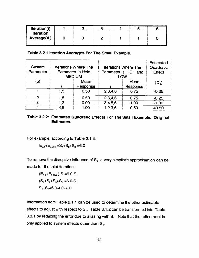
Table 3.2.1 shows the iteration averages for the small example and Table 3.2.2

shows how the iteration averages are wed to estimate the quadratic effects.

l i l

l i I t available

S, i I I 1

1 I not i I , i i available j

i

- - - -

! 1 4

1 Aliased Experirnental Eff ects 1

Table 3.1.2 System Effects As Estimated By The Streamlined Approach

For The Small Example. Original Estimates.

! I

Esürnated 1 Value 1

I I t Neration I

3.3 Refining Estimates of Main Effects And Interactions

A stepwise approach is used refine the estimated main effects and interactions.

1 sl 1 1

I -L 1 h.1 1 -E4.4 i 4% 1 4.0 1 I

/ System i Effect

Accarding to Tables 3.1.1 and 3.1.2. one of the largest system effects is S, and

wnsequentiy S, will be one of the largest sources of error due to aliasing. Given

an estimate of S,, it is possible to reduce the error it induces in estimates of the

other system effects.

1 2 3 4 5 6

iteration(i) 1- I - t - 2 -- 1 - - 3 - l 4 5 1

? - 1

- i - -

Iteration t---- 1 t l i -1 Table 3.2.1 lteration Averages For The Smail Example.

Table 3.2.2: Estirnated Quadratic Effects For The Small Example. Original Estimates.

I 1 Estimated / - Systern lterations Where The 1 Iterationç Where The Quadratic i Parameter I Parameter Is Held 1 Parameter 1s HlGH and 1 Effect 1

I I I MEDIUM LOW I

For example, according to Table 2.1 -3:

&-,+&., =S,+S,+S, =6.0

' (P) i 1 Mean I 1 Response

I

To remove the disruptive influence of S,, a very simplistic approximation can be

made for the third iteration:

(&.1+&.234 )-S,=~-O-SI

(SI +S2+S3)-S S . 0 - S

s2+s,~.o-4.0=~.o

I 1

i I Mean I j Response ,

1 CQ,) :

Information from Table 2.1.1 c m be used to determine the other estimable

effectç to adjust with respect to SI. Table 3.1 -2 can be transformed into Table

3.3.1 by reducing the error due to aliasing with S, . Note that the refinement is

only applied to system effects other than SI.

I 1 I 1.5 1 0.50 2.3.4.6 i 0.75 1 -0.25 /

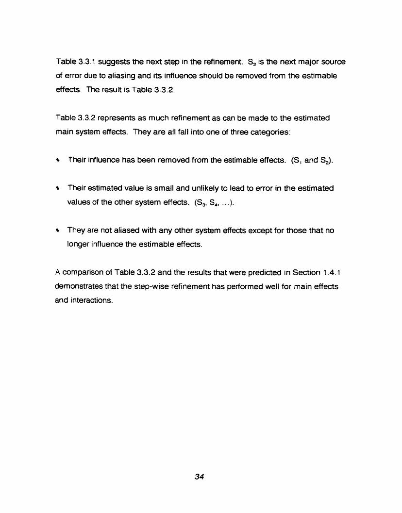
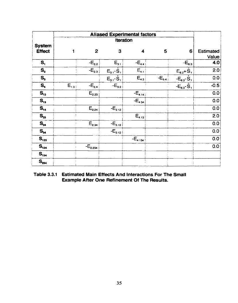
Table 3.3.1 suggests the next step in the refinement S, is the next major source

of error due to aliasing and its influence should be removed from the estimable

effects. The resuIt is Table 3.3.2.

Table 3.3.2 represents as much refinernent as cm be made to the estimated

main system effects. They are al1 fall into one of three categories:

Their influence has ken removed from the estimable effecff. (S, and Sd.

Their estimated value is small and unlikely to lead to error in the estimated

values of the other system effects. (S3, S4, . . .).

They are not aliased with any other system effects except for those that no

longer influence the estimable effects.

A cornparison of Table 3.3.2 and the results that were predicted in Section 1.4.1

demonstrates that the step-wise refinement has performed well for main effects

and interactions.

i I I / Çystem Effect 1 I i Aliased Experimental factors

I

I 1

6

Table 3.3.1 Estirnated Main Effects And Interactions For The Small Example After One Refinernent Of The Results.

Estirnated 1 1 I j S, 6 - 2 ! 6.1 1 4%4 i i ' k . 3

Value I 4.0 1

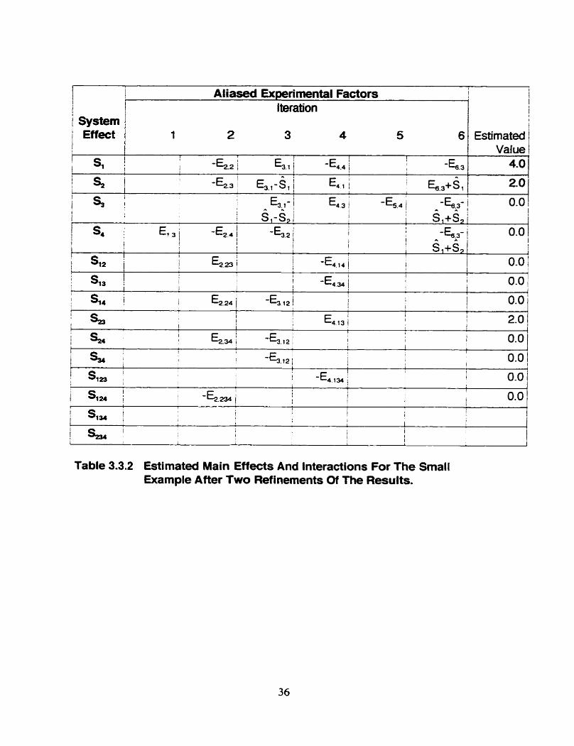
Table 3.3.2 Estimated Main Effects And Interactions For The Small Example After Two Refinements Of The Results.

I Aliased Gcperirnental Factors ! l

I I

1 1

Estimated Value

4-0

i system

i Effect 1

lterahion

2 3 1 4 5 6

; s, i 1

'E22 i 6 . 1 1 -E4.4 ! I

I - 4 3

3.4 Refining Estimates of Quadratic Effects

Just as the estimates of the main effects were refined by adjusting the estimable

effects, the estimates of the quadratic effects can be refined by adjusting the

iteration averages. From Table 3.2.2, it appears the largest quadratic effect is

Q,. The average response for iterations 1 and 2 can be adjusted to remove the

estimated influence of Q,. Tables 3.4.1 and 3.4.2 show the result of the

adjustment. The row for Q, is shaded because it shows results from a previous

estimate.

Table 3.4.1 lteration Averages For The Small Example After One Ref inement.

Iteration(i) Iteration

Average(A3

1 1 2 ! 3 j 4 j 5 / 6 0-6, O - 1 1 1

1 i 1 1 2 1 1 i l i 0 I i 1 I

I i

Table 3.4.2 Estimated Quadratic Effects For The Small Example After One Refinement.

1

1 1 \ ! I ! Estirnated 1 i I Systern lterations Where The i lterations Where The / Quadratic j

i 1 Parameter ) Parameter 1s Held Parameter Is HlGH and 1 Effect 1 l

I , MEDIUM i LOW 1 1

' j (P) i ! Mean 1 i Mean 1 1

1 l 1 <a,> 1 ; Response 1 I ; Response 1

1

I 1 1,5 1 1-00 1 2.3,4,6 [ 1.00 1 0.00 j f

2 i 1,5 t I

I 3 1 2 1 .O0 0.00 1.00 I -1 .O0 1.00 / 0.00 l

I 4 i 4,5

1-00 ! 2,3,4,6 0.00 1.00

3.41516 1,2,3,6 -

Chapter 4

Confidence Coefficients And Confidence Bounds ln The SWAC3-CC3

Example

4.1 The Estimated Effects

The calculations made for the small example are very transferable to the

SYVAC3-CC3 example. However, the sheer number of effects prevents the

luxury of a cornplete description of the aliasing structure as was done in

Table 2.1 -3. Fortunately. calculations such as those in Table 3.1.2 are possible.

Also, even for a system as large as SYVAC3-CC3 it is practical to estimate al1

the main effects and al1 the quadratic effects.

Table 4.1.1 shows the largest estimated main effects and Table 4.1 -2 shows the

largest estimated quadratic effects as determined from the initial estimates.

Of concern are the columns labeled "Actual Effect". The information in these

columns is based on expert knowledge of SYVAC3-CC3. According to expert

knowledge, many of the system parameters (number 1927 for example) can

have no influence on the measured response of the system but the S, and Q,

columns suggest some of these parameters do have effects.

In Tablas 4.1.1 and 4.1.2, CL,(S,), c&(s,), CLQ,(Q,) and CQLJQ,) represent

confidence coefficients and CB(S,) and CBQ(Q,) are confidence bounds.

Sections 4.2 and 4.3 will discuss confidence coefficients and confidence bounds.

The estimated effects can be revised as was done in Sections 3.3 and 3.4.

4.2 Main Effects and Interactions

For the SYVAC3-CC3 example. it is possible to assign confidence bounds and

confidence coefficients for the system effects. These assignments are based

upon the assumption that the estimable effects have a Normal distribution.

Normal distributions are not unexpected s ine a estimable effect is approximately

the sum of a random set of systern effects and the Central Lima Theorem is likely

to take effect. As will be shown. this assurnption can be easily supported

through probit plots.

To look at the distribution of the estimable effects, there is a useful property of

the sub-design used in the SYVAC3-CC3 example :

The estimable effects can be divided into two mutually exclusive sets; one

is aliased with odd-ordered interactions (including main effectç) and the

other is aliased with even-ordered interactions.

This property is a result of the aliasing structure used in the sub-design

which in cornmon notation (Montgomery 1991 ) can be expressed as:

1 .O00 1 .O00 0.334 Yes 1 .O00 1 .O00 0.358 ves

Table 4.1.1 : The Largest Main Effects For SWACSCC3. Original Estimates.

Table 4.1.2: The Largest Estimated Quadratic Effects For SWACSCC3 . Original Estimates.

Figure 4.2.1 consists of a probit plot for both of the groups of the estimable

effects. Bath appear to have an approximately Normal distribution.

Either of these two groups is expected to have a mean of zero. In the

assignrnent of system parameters to experimental factors, there is an equal

probability of a system parameter and an experimental factor moving in the same

or opposite direction and consequently there is an equal probability that a system

effect will be added to or subtracted from a estimable effect.

The standard deviations of these hivo groups. STDEV,, and STDEV,,, are

readily estimated from the samples of values.

There is now enough information to predict the distribution of the estimated main

effects and interactions of the system parameters. If these effects are simply

averages of random estimable effects. the expected distribution is:

where:

s is the main effect or interaction

N is the number of iterations used to calculate s STDEVE~~,, 1s STDEVE(,~I ., STDEV,,, depending on the order of the

interaction

t,, is the students t-variate with N-1 degrees of freedom

Confounded with Odd-Ordered Interactions

Estimable Effect

Confounded with Even-Ordered Interactions

/'* 7'

1 I I I 1 I 1

O

Estimable Effect

Flgure 4.2.1 : Dlstrlbution Of Estimable Effects.

Original Estimate of Main System Effects

Estimated Main System Effects

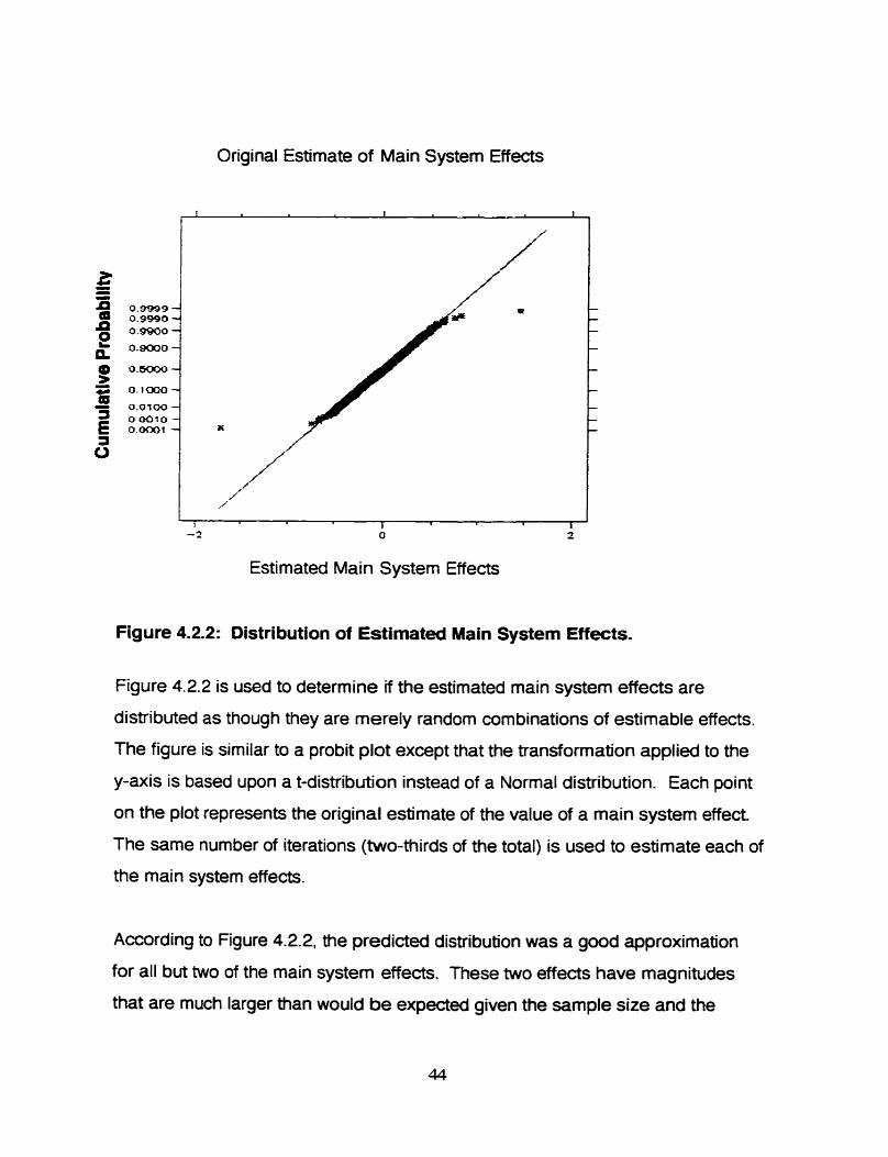
Figure 4.2.2: Distribution of Estimated Main System Effects.

Figure 4.2.2 is used to determine if the estirnated main systern effects are

distributed as though they are rnerely randorn combinations of estimable effects.

The figure is similar to a probit plot except that the transformation applied to the

y-axis is based upon a t-distribution instead of a Normal distribution. Each point

on the plot represents the original estimate of the value of a main system effect

The same number of iterations (two-thirds of the total) is used to estimate each of

the main system effects.

According to Figure 4.2.2, the predicted distribution was a good approximation

for al1 but two of the main system effects. These two effects have magnitudes

that are much larger than would be expected given the sample size and the

predicted distribution. The figure gives us confidence that these two main

system effects are not occurring randomly and instead represent actual effects

that occur in the system.

It is also possible to calculate confidence coefficients for the estimated system

effects. A suitable nuIl hypothesis is:

Ho: The system effect (main or interaction) is zero. S=û

Two variations on the confidence coefficient are necessary; one is useful for

single effects and the other is useful for screening a large number of estimates

for statistical significance.

To test individual estimates, very standard methods are available. A t-variate

corresponding to the estimated effect is calculated and a pvalue is generated.

Corresponding confidence coefficients are assigned and listed in the table as

CL,( SPI-

Table 4.1 -1 also demonstrates why cL,(s) is inappropriate for screening a large

number of effects for statistical significance. To produce the table. approximately

3300 main linear effects were screened. The expected number of estimated

main system effects to be declared 99% significant on a purely spurious basis is

(1 % '3300) -33. In Table 4.1 -1, there are many system parameters known to

have no influence on the system response (expert judgement) and yet by CL,(S)

they appear significant It is useful to have a confidenœ coefficient that

considers the number of estimates that are tested.

where

N, is the number of effects tested for statistical significanœ

is such a value. Under the predicted distribution. it is a first-order approximation

to the probability that al1 mernbers of the sample are smaller than the tested

estimate.

CL(S) values are also included in Table 4.1 -1 . Under Mis coefficient, only two

system effects achieve a 99% tevel of confidence. These two effects are

consistent with expert knowledge of SYVAC3-CC3. However, according to expert

knowledge. some of the other parameters in Table 4.1.1 should also have

significant main effects.

The cl&) values are more consistent with knowledge of SYVAC3-CC3 than

the CL,(S) values but they are still not entirely satisfactory. However, as the

estimable effects are modified to refine the estimated effects, the cunfidence

coefficients and confidence bounds are also recalculated and the results are

expected to improve.

How accurate are the estimates of S? We can find CB(S) such that s r CB(S)

forrns the 95% confidence bound. We assume:

STDEV . - t N - 1

€ 1 Si

where

s is the estimated system effect -

Err(S) is the error made in estirnating S

N is the number of iterations used to estimate S

STDEVEf& is an estirnate of the standard deviation of the rneasurable effects

after the estimated influence of S has been removed.

STDEV,, i, is ctosely related to STDEV,, or STDEV,,, depending on the

order of S. For example, STDEVEtL, is the same as STDN,,, except that:

*

E, , + S, is used instead of E, , E2.8 + ~ 2 2 3 9 is used instead of E2.8

E63 - 52239 iç used instead of E63

etc.

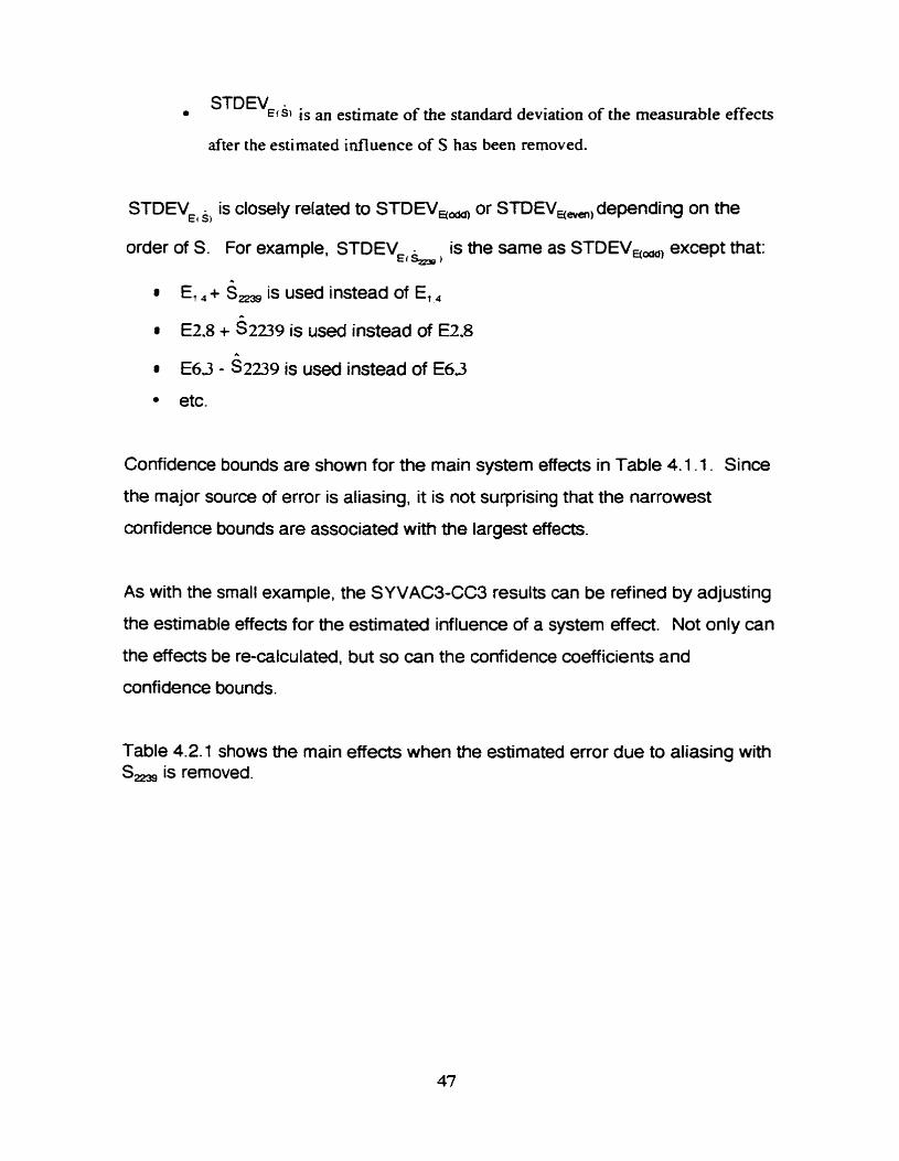
Confidence bounds are shown for the main system effects in Table 4.1 -1. Since

the major source of error is aliasing, it is not surprising that the narrowest

confidence bounds are açsociated with the largest effectç.

As with the small example, the SYVAC3-CC3 results can be refined by adjusting

the estimable effects for the estimated influence of a system effect. Not only can

the effects be re-calculateci, but so c m the confidence coefficients and

confidence bounds.

Table 4.2.1 shows the main effects when the estimated error due to aliasing with S, is removed.

P S. CL&) &(S.) CB(SJ Effect 2239 -1 -725 1.000 1.000 0.334 YeS 2443 1.533 1 .O00 1 1 .O00 0.262 Yes 2355 0.732 1 .O00 0.732 0.319 Yes 2803 0.608 0.999 0.08 O 0.324 Yes 2992 0.5 5 5 0.998 0-002 0.326 no

1 04 0.55 1 0.998 0.002 0.326 Yes 2712 0.5 1 1 0.996 0.000 0.327 no 2026 0.499 0.996 0.000 0.327 no 2796 0.49 5 0.995 0.000 0.3 27 no 328 0.475 0.994 0.000 0.328 no

2856 0.4 7 2 0.993 0.000 0.328 no 2448 0.469 0.993 0.000 0.328 no

1272 -0.469 0.993 0.000 0.328 no

2793 0.467 0.993 0.000 0.328 no

376 0.464 0.993 0.000 0.3 28 no

2826 -0.460 0.992 0.000 0.3 28 Yes 1 0.45 7 0.992 0.000 0.329 no

2588 0.446 0.990 0.000 0.329 no 1152 -0.438 0.989 0.000 0.3 29 no 405 0.436 0.989 0.000 0.329 no 1612 -0.434 0.988 0.000 0.329 no 3290 -0.43 1 0.988 0.000 0.329 no

Table 4.2.1 : The Largest Estimated Main Effects For SWAC3-CC3 After One Revision.

Actual P S. CL&) CI&,) CB(S,) Effect

I 2239 -1 -725 1.000 1 1 -0ao 1 0.334 1 Y s 2443 1.533 i .ooot r.ml 0.262 1 Y= 2355 0.655 7 .O00 0351 f 0.247 Y- "

2803 0.608 1 .O00 0.94 1 0.232 Yes 1461 0.41 4 0.999 0 .O44 0.225 no

Table 4.2.2: The Largest Estimated Main Effects For SWAC3-CC3 After Three Revislons.

Table 4.2.1 suggests that the next refinement to make is to adjust the estimable

effects to remove the estimated error due to aliasing with S,-. And of course

the step-wise refinement can continue. Table 4.2.2 shows the results after three

refinements are made.

After three refinements of the results, there are no more main effects that are

statistically significant (confidence coefficient greater than 95%) according to

CL(S) However, the information in Table 4.2.2 suggests some non-zero main

effects are not signlicant according to cLJs). According to expert knowledge,

S,,S,,S,,S,, and S, ,, could be non-zero. According to CL, ( s), their

estimated effects are statistically significant but so is s,,, which is known to

have no achial effect. Chapter 5 will discuss how expert knowledge can be

incorporated into the application of IFFDA.

When confidence coefficients and confidence bounds are calculated for

interactions, the only special concern is that a variable number of iterations of the

sub-design are used to estirnate the interactions.

4.3 Quadratic Effects

Confidence coefficients and confidence bounds can also be calculated for the

quadratic effects. The methods are very analogous to those used for main

effects and interactions.

Quadratic effects are estimated from the mean responses as calculated for the

iterations of the sub-design(Section 3.2). The Central Limit Theorem suggests

that the iteration means could have a Normal distribution. Figure 4.3.1 is a probit

plot of the iteration means for the SYVAC3-CC3 example and shows that the

distribution is at least approximately Normal.

If the estirnated quadratic effects are created from random combinations of

iteration averages, then they are expected to be transformable to a Student-t

distribution.

where

Q, is the estimated quadratic effect of parameter p

is the number of iterations where parameter p is included in the

sub-design

&, is the number of iterations of the sub-design

STDEV, is the standard deviation of the iteration rneans

t w is the Student-t distribution with - 2 degrees of freedom.

There are - 2 degrees of freedom because two values are required

to estimate a difference,

Figure 4.3.2 is a graphical test of whether the estimated quadratic effects have

the predicted distribution. It is similar to a probit plot except that the

transformation on the y-axis is based upon a Student-t distribution instead of a

Normal distribution. Very low and very high Q, values do not occur as frequently

as predicted. However, the predicted distribution is close and will be assumed

for the rest of the calculations.

A suitable nuIl hypothesis is:

Ho: The quadratic effect is zero. Q,=U

As for the main effects, two variations of a confidence coefficient will be used.

CLQ,(Q,) uses standard p-values and is suitable for testing individual quadratic

effects. CLO,(Q,) is suitable for screening a large number of quadratic effects

for statistical significance. The relationship between the two coefficients is:

where

N, is the number of effects tested for statistical significanœ

Table 4.1.2 includes the confidence coefficients for the largest quadratic effects

in the SYVAC3-CC3 example. None of the quadratic effects are statistically

significant under CLQ,(Q,). However, this is not to say there are no achial

quadratic effects. As shown with the linear effects, confidence coefficients such

as c ~ ( s ) and CLQ,(Q,) are very restrictive due to the large sarnple sizes. If a

justification can be found to use CLQ,(Q,) for some of the paramelers. the

estimated effects may be significant.

It is convenient to apply CLQ,(Q,) to sets of one hundred system parameters.

For a set of one hundred CLQ,(Q,) values, the expected number of effects to

falsely appear significant (CLQ, ( ÔP)>99% ) is manageable (-1 ).

The obvious parameters to test for significant quadratic effects are those with the

largest linear effects. Two assumptions are required to justify this choice:

The system parameters with the largest quadratic effects also have the

largest linear effects.

The error in the estirnated quadratic effects occur independently of the

error in estimating the linear effects.

Therefore we can test the 100 system parameters with the largest linear effects

to see if their quadratic effects are significant Or these 100 quadratic effects.

Table 4.3.1 shows the largest ones. Even if the quadratic effects are tested

individually, no statistical significance (990h confidence coefficient) can be

attributed to any of these 100 quadratic effects. As was the case for the main

effects. the user has the option of spending more resources to further investigate

the quadratic effects of any suspicious parameters.

The confidence bounds for the quadratic effects. CBQ( Q,) can of course be

calculated. The methodology is very similar to that used for the linear effects.

We use the assurnption that:

STD EV,. , p, - hW -2

where:

ERR(&) is the error in the estimate of Q,

2 is the Student-t distribution with b, - 2 degrees of freedom

STDEV,.,,, is the standard deviation of al1 A, values without the

estimated influence of O,

STDEV, is transfoned into STDNx,p, by modQïng A, values that are affected

by Q,. Using parameter number 2239 from the example: CI

A, - Q, will be used instead of A, *

A,- Q, will beused instead of A,

etc

The estimated 95% confidence bounds are included in Table 4.1 -2

Iteration Averages

1

-8 s -go -7-5 -7 O - 6s Average System

Responses

Figure 4.3.1 : Distribution Of Average Responses From lterations Of The SubDesign.

Original Estimate of Quadratic System Effects

Estimated System Quadratic Effects

Figure 4.3.2: Distribution Of Estimated Svstem Quadratic Effects.

CHAPTER 5 Applying The Calculations To A Large System

Previous sections have discussed the calculations that are made as part of

I FFDA. However, there are other issues that must be resoived for l FFDA to be

applied to a large system such as S WAC3-CC3.

In what order should the system effects be removed from the estimable

eff ects or the system averages so that the results can be refined?

Which system effects should be reported?

The following assumptions are made to deal with these issues:

The easiest system effects to detect are the main effects.

Any parameter with a significant quadratic effect or involved in a

significant interaction will also have a relatively large main effect.

The error in estimating main effects, quadratic effects and interactions

occur independently.

Under these assumptions it is still necessary ta screen the system parameters to

determine which ones may be important. As a result. some systern effectç will

have to be subjected to the more restrictive tests of statistical significance.

cLJs) and CLQ,(Q). However, the screening will also provide the basis for

identifying other system effects to test individually with the l e s restrictive tests of

significance, CL,(S) and CLQ,(Q).

It is convenient to apply CL, (s) or CLQ, (6) to sets of approximately one

hundred estimated system effects. W hen a set of one hundred system effects

are tested with cL,(s) or CLQ,(Q), approximately one of them will be assigned

statistical significance (confidence coefficient greater than 99%) even though it

isn't actually significant. If too many estimated effects are tested. then a large

number of the effects will appear significant on a purely spurious basis. If too few

effects are tested. then more significant effects will be missed because they were

not tested.

The steps for the analysis of results of the experimental design can be

summarized as follows:

1. Screen al1 the main effects (S,) to determine which estimates are

statistically significant (see Sections 3.1 and 3.3). The step-wise

refinement of the results is applied as statistically significant estimates

are identif ied.

2. Screen al1 the quadratic effects (Q,) to deetmine if any estimates are

statistically significant. (see Sections 3.2 and 3.4). The iteration

averages are adjusted as statistically significant system estirnates are

identified.

3. Take the 100 system parameters with the largest main effects

(significant or not) and test their quadratic effects individually. Record

any Q, values that are statistically signlicant when tested individually

and adjust the experimental averages accordingly.

4. Select 15 system parameters to test for statistically significant second

order interacûons. These 1 5 parameters include:

the pararneters wiai statistically significant main effects

the parameters with statistically significant quadratic effects

enough of the parameters with the largest non-signlicant main

effects to bring the total number up to 15

All 105 possible pairs of these system parameters are tested

individually for statistical significance (C hapters 3 and 4). Adjust the

estimable effectç to acknowledge these significant effects.

5. Select 10 system pararneters to test for statistically significant third

order interactions. These 10 parameters include:

the parameters with statistically significant second order

interactions

the parameters with statistically significant main effects

the parameters with statistically significant quadratic effectç

enough of the parameters with the largest non-signlicant main

effects to bring the total number up to 10

All 120 possible third order interactions are tested individually for

statistical significanœ. Adjust the estimable effects to acknowledge

these significant effects.

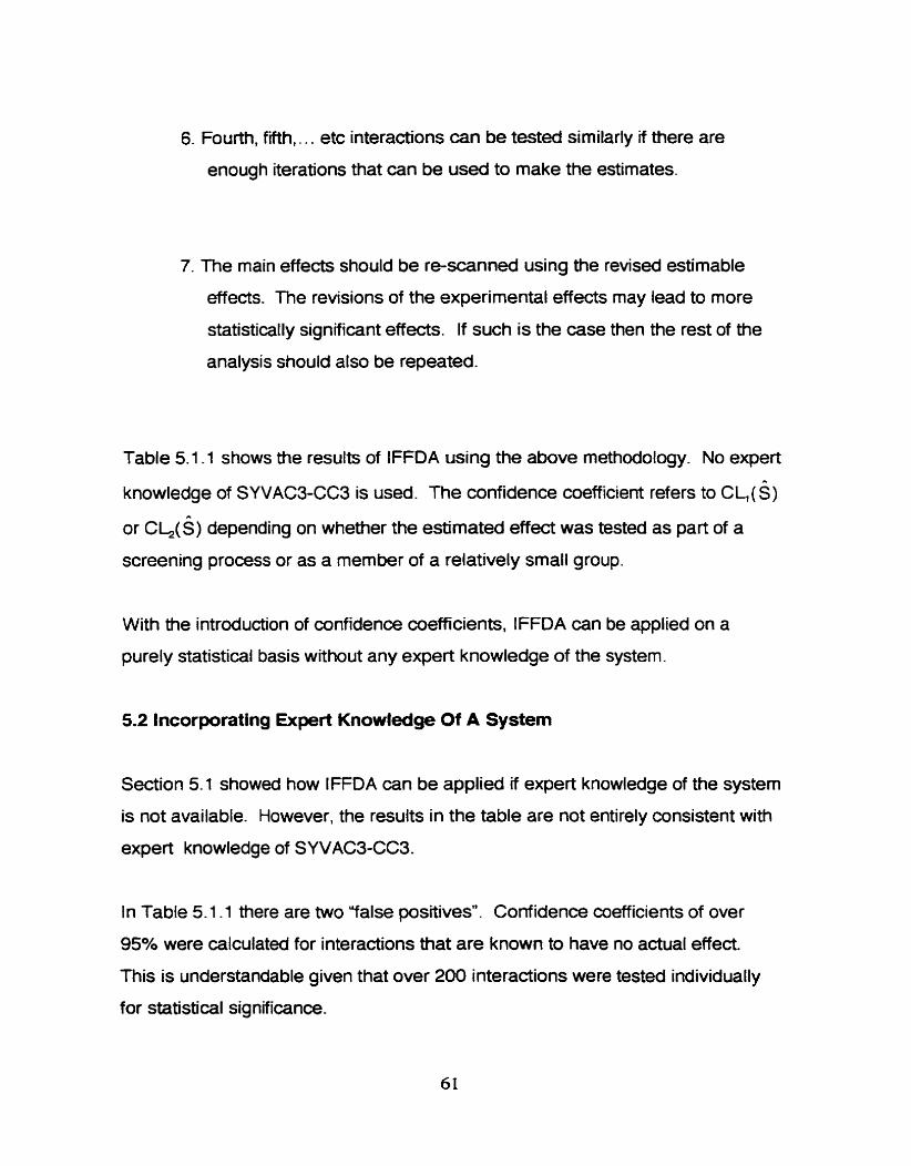
6. Fourth, fiih,. . . etc interactions can be tested similarly if there are

enough iterations that can be used to make the estimates.

7. The main effects should be re-scanned using the revised estimable

effects. The revisions of the experimental effects may lead to more

statistically signlicant eftects. If such is the case then the rest of the

analysis should also be repeated.

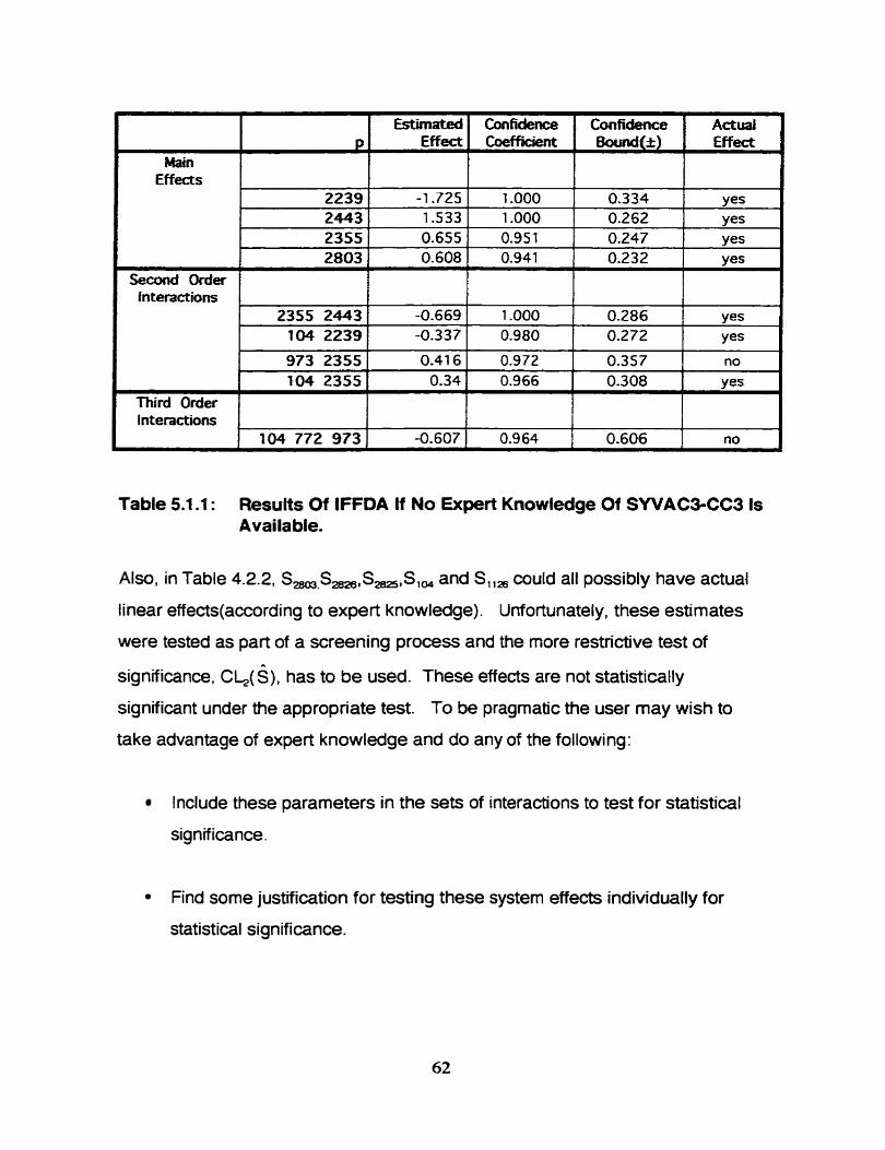
Table 5.1 -1 shows the results of IFFDA using the above methodology. No expert

knowledge of SYVAC3-CC3 is used. The confidence coefficient refers to C ~ ( S )

or c ~ ( s ) depending on whether the estimated effect was tested as part of a

screening process or as a member of a relatively small group.

With the introduction of confidence coefficients, IFFDA can be applied on a

purely statistical basis without any expert knowledge of the system.

5.2 lncorporating Expert Knowledge Of A System

Section 5.1 showed how IFFDA can be applied if expert knowledge of the system

is not available. However, the resuRs in the table are not entirely consistent with

expert knowledge of SYVAC3-CC3.

In Table 5.1 -1 there are two "false positives". Confidence coefficients of over

95% were calculated for interactions that are known to have no actual effect.

This is understandable given that over 200 interactions were tested individually

for statistical significance.

1 2355 2443 1 -0.669 1 1.000 1 0.286 1 ves

1

P Effect Coefficient Ef fect I Main

Eff ects

Table 5.1.1 : Results Of IFFDA If No Expert Knowledge Of SWAC3-CC3 Is Availa ble.

Third Order Interactions

linear effects(acc0rding to expert knowledge). Unfortunately. these estimates

1

2239 2443 2355 2803

were tested as part of a screening proces and the more restrictive test of

973 2355 104 2355

104 772 973

significance. c ~ ( s ) , has to be used. These effects are not statistically

-1.725 1.533 0.655 0.608

significant under the appropriate test. To be pragmatic the user may wish to

0.41 6 0.34

-0.607

take advantage of expert knowledge and do any of the following:

1.000 1 -000 0.95 1 0.94 1

lnclude these parameters in the sets of interactions to test for statistical

significance.

0.972 0.966

0.9 64

Find some justification for testing these system effects individually for

statistical significance.

0.3 34 0.262 0.247 0.232

Yes Yes Yes Yes

0.357 0.308

0.606

no

Yes

no

Do further analysis using more simulations to look specifically at these

system effects.

lncrease the number of iterations of the sub-design and repeat IFFDA.

Repeat the analysis with a different objective function.

The first option will be discussed here.

For SYVAC3-CC3. the influence of the majority (at least 2000) of the system

parameters can be dismiççed on the basis of expert knowledge. In such a

situation. expert knowledge is very valuable. In fact, previous applications of

IFFDA depended entirely on expert knowledge to guide the refinement of the

results. For example:

The estimated effects in Table 4.2.2 suggests that system parameter

number 1461 has an influence on the estirnated dose rate. However,

according to expert knowledge of SYVAC3-CC3. this system parameter

is assigned a constant value and cannot contribute to the variability of the

dose estimate. On this basis, we have no confidence that parameter

nurnber 1461 has any sort of influence on the systern response.

Also, Table 4.2.2 suggests that one of the largest system effects is S,.

Expert knowledge gives no simple reason why S, can't be important.

In the previous applications of IFFDA, there confidence coefficients were

not used and S, would warrant further analysis to determine its effect

on the system.

The oppominity to incorporate expert knowledge cornes in the choie of

quadratic effectç and interactions to test individually. lnstead of just using the

system parameters with the largest estimated main effects, we can be selective

and give preferenœ to those system parameters expected to have an influence

on the system.

For example, when Table 4.2.2 is used to identify system parameters to check

for second order interactions, the selection can be restricted to those marked

"y& in the Actual Effect column. This approach only gives eight parameters but

the table could be extended to get more systern parameters to test for second

order interactions.

Table 5.2.1 shows the results if the estimated interactions associated with the

eight parameters are tested for significance. Parameters 104, 1 126, 2803 and

2826 are involved in statistically significant interactions. They can be considered

important to the system even though there is no statistical reason for believing

their main effects are significant.

However, we are still have not found any statisticaliy significant estimate

associated system parameter number 2825. With the amount of data that is

used in the example (30 iterations of the sub-design), there is no statistically

justifiable reason for saying that this systern parameter has an influence on

SYVAC3-CC3.

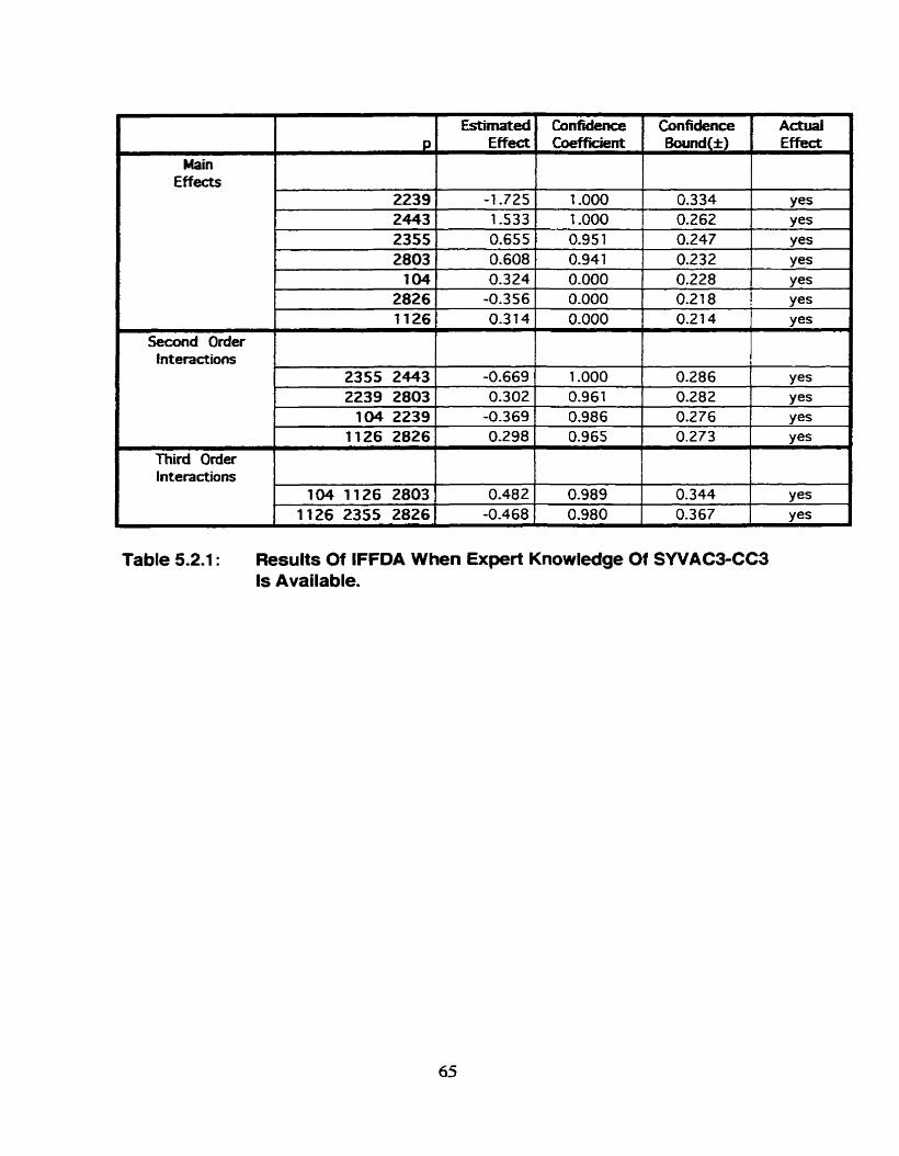
1 1 1 Estimatedl Confidence f Confidence 1 Actual

Main

r - 2826 3 -0.356 1 0.000 1 0.21 8 1 yes

Effects

r- 11261 0.3141 0.000 1 0.214 1 yes

P

Second Oder 1 1 1 1 1

2239 2443

Eff-

Interactions I I I

-1.725 1.533

fnteractions

Table 5.2.1 : Results Of IFFDA When Expert Knowledge Of SYVAC3-CC3 Is Available.

Coefficient

1 -000 r -000

2355 2443

Bound(I) Ef fect

0.334 0.262

1 -0.669 1 1 .O00

Yes Y=

0.286 yes

CHAPTER 6 Conclusions

The ability to calculate confidence bounds and confidence coefficients for the

results of IFFDA has been demonstrated. Sample calculations have k e n used

to dernonstrate this capability.

With confidence bounds and confidence coefficients, IF FDA can be applied

without any expert knowledge of the system, but in the SWAC3-CC3 example,

IFFDA gives better results if expert knowledge of the system is incorporated into

the analysis.

CHAPTER 7

Recommendations

lterated Fractional Factorial Analysis (IFFDA) has already proven itself to be a

powerful tool for the sensitivity analysis of computer models. This report

illustrates how the introduction of confidence bounds and confidence coefficients

enhance the value of IFFDA. Five further steps are possible to increase the

effectiveness of IFFDA:

1. lnvestigate Variations On The Experirnental Designs To Optimize Results.

2. Incorporate Better Statistical Methods To Estimate The Confidence

Coefficients For The Estimated System Effects.

3. lnvestigate Using ANOVA To Screen The Main Effects and Interactions.

4. lnvestigate The Influence Of Aliased System Effects On the Estirnated

Quadratic Effects.

5. l ncorporate The Analysis Stage Of IFFDA lnto A Fonal Software

Package.

7.1 lnvestigate Variations On The Experirnental ùesigns To Optimlze

Results

lt is desirable to optimize the designs uçed in IFFDA to maximize the amount of

information that can extracted from a given amount of data. Even for cornputer

simulations, data can be expensive to generate. For a given number of

simulations, the following features of the experimental designs are still

adjustable:

The definition of LOW. MEDIUM and HlGH for the system parameters.

The choice of sub-designs

The sub-design in the sample calculations is a 284fractional factorial

design. IFFDA could be generalized to accommodate any other sub-

design.

The obvious sub-designs to consider are other two-level fractional

factorial designs.

The number of iterations of the sub-design.

If the sub-design is changed, the number of simulations per

iteration will change and more or fewer iterations will be possible

with the same total number of experirnents.

7.2 tncorporate Better Statistical Methods To Estimate The Confidence

Coefficients And Confidence Bounds

The statistical meaiods in this report use the assumption that the measurable

effects and the iteration averages have an approximately Normal distribution.

The approximation appears to be more valid for the estimable effects than the

iteration averages (Figures 4.2.1 and 4.3.1 ). As a result. there is a concern that

in future applications of IFFDA, the assumption of Normal distributions would not

be suitable. In such a situation, some of the statistical methods used in this

report would not be valid. Other statistical methods may have to be found.

For CL,(S), CLQ,(Q), CB(S), and CBQ(Q), a simple non-parametric is possible.

A large number (thousands) of "pseudo system parameters" could be generated

and assigned to experimental factors. Since the effects of these pseudo

parameters would be zero, their estimated effects can be used to estimate the

error which is likely to occur in the estimated effects of the actual system

parameters. Confidence coefficients and confidence bounds could be generated.

Unfortunately, this approach would be impractical to replace CL(S) and

CLQ,(Q). Millions of the pseudo system parameters would be required.

7.3 lnvestigate Using ANOVA To Screen The Main Effects And

Interactions

It may be possible to use one-way ANOVA to estimate main effects and

interactions. It may also be possible to treat the iterations of the sub-design as

experimental blocks. A block would represent an alias structure whereas in

most experimental designs a block represents something physical (a plot of

ground or a petri dish) or a period of tirne.

In order to revise results, responses of individual experiments would be adjusted

instead of the measurable effects.

The major advantage of this approach would be that standard statistical methods

could be used to analyze the results.

7.4 Investigate The Influence Of Aliased System Parameters On the

Estimated Quadratic Effects

For the estirnates of the quadratic effects, the iteration averages were adjusted

with respect to the most significant estimated quadratic effects. However, the

iterations are possibly influenced by interactions as well.

If a group of system parameters is aliased in an iteration. then their interaction

will remain at a constant level instead of toggling between LOW and HIGH.

As a result, the average response for the iteration may be raised or lowered due

to interactions between system parameters that are aliased together.

Consequently, estimated quadratic effects will also be influenced.

This concern should be further investigated and i f warranted. IFFDA should be

modified to reduce the influence of interactions on the iteration averages and

estimated quadratic effects.

7.5 Incorporate The Analysis Stage Of IFFDA lnto A Formal Software

Package

Cornputer software to generate the designs for IFFDA has been created.

However, at this time. the development of software to perform the analysis part of

IFFDA is still in a prototype phase.

When software is further developed to perform the analysis part of IFFDA.

confidence coefficients and confidence bounds should be inwrporated. Not only

do these values put the results of IFFDA in better perspective, they also provide

some objective guidance when the user is revising results to reduce error due to

aliasing between system eff ects.

Bibliography

Andres, T.H. 1997. Sampling Methods and Sensitivity Analysis for Large Parameter Sets. Journal of Statistics and Computational Simulations. Vol. 57. pp77-110, 1 997

Andres. T.H. and Hajas. W.C. 1993. Using Fractional Factorial Design to Screen Parameters in Sensitivity Analysis of a Probabilistic Risk Assessment Model. Joint International Conference on Mathematical Methods and Super computing in Nuclear Applications, Karlsruhe, Germany, 1993

Gwdwin, B.W., T.H. Andres, Hajas. W.C.. LeNeveu,D.M.. . Melnyk, T.W.. J.G. Szekely, Wikjord.A.G., Donahue,D.C., Keeling,S.B., Kitson.C.1. ,Oliver.SE. Witzke,K. and Wojciechowski,L.. 1996. The Disposal of Canada's Nuclear Fuel Waste: A Study of Postclosure Safety of In-Room Emplacement of Used Candu Fuel in Copper Containers in Permeable Plutonic Rock. Volume 5: Radiological Assessment. Atomic Energy of Canada Limited Report, AECL-11494, COG-95-552- 5

Goodwin.B. W.. McConnel.D.8.. Andres.T.H.. Hajas. W.C.. LeNeveu.D.M.. Melnyk.T.W., Sherman,G. R.. Stephens. M.E., Szelely. J.G.. Bera.P.C.. Cosgrove.C. M.. Dougan,K.D., Keeling,S.B., Kits0n.C. 1.. Kummen.B.C., Oliver,S.E., K. Witzke, Wojciechowski, L. and Wi kjord, A.G. 1 994. The Disposal of Canada's Nuclear Fuel Waste: Postclosure Assessment of a Reference System. Atornic Energy of Canada Limited Report, AECL- 1 071 7, COG-93-7

Iman. R.L. and Conover. W. J. 1 980. Small Sample Senstivity Analysis Techniques for Computer Models, with an Application to Risk Assessment. Communications in Statisctical Theory and Methodology, A9(17), pp 1 749-1 842 1 980.

Kliejnen. J.P.C. 1 992. Sensitiwty Analysis of Simulation Experiments: Regression Analysis and Statistical Design. Mathematics and Corn puters in Simulation. Vol. 34. 1 992. pp 297-31 5.

Montgomery. Douglas,C., 1 991 . Design and Analysis of Experiments. Third Edition. John Wiiey and Sons, 1991

Saltelli. A., Andres. T.H. and Homma,T. 1995. Sensitivity Analysis of Model Output. Performance of the lterated Fractional Factorial Design Method . Com putational Statistics and Data Analysis. Vol. 20, pp387-407. 1995

SaReIli, A.. Andres. T. H. and H0mma.T. 1 993. Sensitivity Analysis of Model Output. An lnvestiigation of New Techniques.Computational Statistics and Data Analysis. Vol. 1 5, pp 21 1 -237. 1 993

Appendix

Glossary of Terms and Symbols

A 4

the mean of the response for the ith iteration of the sub-design

ms1 the confidence bounds for a main effect or interaction

~t CB(S) forms the 95% confidence band

the confidence bound for Q

~t CBQs ( Q ) forms the 95% confidence band

CL1 (SI

the confidence coefficient for S if it is tested as an individual effect

CU ( s r the confidence coefficient for s if it is tested as part of a screening of many

eff ects

the confidence coefficient for Q if it is tested as an individual effect

the confidence coefficient for Q if it is tested as part of a screening of many

effects

indeces used to identfy experimental effects

Ei. e

effect of experimental factor e in iteration i of the sub-design

Ei.e 1 .e2 e3.. . .

interaction of experimental factors e l . e2. e3 ... . in iteration i of the sub design

eff ects :

the response of the system to a change in the value of a systern parameter or

an experimental factor

in particular

i f

x, are parameters normalized to a range of [O, 1]

y is the system response

y-L,'x, + q'x& + r*x,'x,

then

LI, L, are main effects

-.25'q is a quadratic effect

.5'r is an interaction of order 2

estimable effect

an effect that can be estimated from an experimental design

typically. aliasing occurs in the design and the estimable effect represents a

combination of many effects

experimental desian

a methodical way of setting parameter values in order to optimize the

resulting information about the system

in IFFDA, the experimentai design consists of iterations of a sub-design

experimental factor

a construct used in IFFDA

ievel set according to a sub-design

represents a different set of systern parameters in each iteration of the sub-

design

its effects are assumed to be a sum of the effects of its member system

parameters

an index used to identify iterations of the sub-design

N. -.= the number of effects being tested for statistical significance

N -2

the number of iterations where a system parameter is included in the sub-

design

QP the quadratic effect of system parameter p

e parameter number

an index used to identw the system parameters

S the linear effect of system parameter s

STDEV, -

the standard deviation of the Ai values

S T D E V , t , , , n , the standard deviation of measured experirnental effects that are aliased with

odd/even ordered interactions

STDEV,

the standard deviation of estimable effects without the contribution of S.

STDEV,

the standard deviation of the iteration averages without the contribution of Q,.

sub-desion

a relatively small and standard experimental design

typically in IFFDA the sub-design is a 2- fractional factorial design

fractional factorial design

svstem

the entity being analyzed

in the sarnple calculations it is a mathematical or computer model but a

system could be a manufacturing or a biological proœss

svstem parameter

something in the systern that can be controlled

IMAGE EVALUATION TEST TARGET (QA-3)

A P P L I E O IMAGE. lnc - - - 1653 East Main Street - -. - - Rochester. NY 14609 USA -- -= Phone: 716/482-0300 -- -- - - F a : 716t288-5989