Cones of matrices and setfunctions,and 0-1 optimization

L. LovaszDepartment of Computer Science, Eotvos Lorand University,Budapest, Hungary H-1088,andDepartment of Computer Science, Princeton University,Princeton, NJ 08544

A. SchrijverMathematical Centre, Amsterdam, The Netherlands

(Revised September 1990)

Abstract. It has been recognized recently that to represent a polyhedron as theprojection of a higher dimensional, but simpler, polyhedron, is a powerful tool in poly-hedral combinatorics. We develop a general method to construct higher-dimensionalpolyhedra (or, in some cases, convex sets) whose projection approximates the convexhull of 0-1 valued solutions of a system of linear inequalities. An important feature ofthese approximations is that one can optimize any linear objective function over themin polynomial time.

In the special case of the vertex packing polytope, we obtain a sequence of systemsof inequalities, such that already the first system includes clique, odd hole, odd anti-hole, wheel, and orthogonality constraints. In particular, for perfect (and many other)graphs, this first system gives the vertex packing polytope. For various classes of graphs,including t-perfect graphs, it follows that the stable set polytope is the projection of apolytope with a polynomial number of facets.

We also discuss an extension of the method, which establishes a connection withcertain submodular functions and the Mobius function of a lattice.

1980 Mathematics subject classification: 05C35, 90C10, 90C27. Key words andphrases: polyhedron, cone, vertex packing polytope, perfect graph, Mobius function.

1

0. Introduction

One of the most important methods in combinatorial optimization is to representeach feasible solution of the problem by a 0-1 vector (usually the incidence vector ofthe appropriate set), and then describe the convex hull K of the solutions by a systemof linear inequalities. In the nicest cases (e.g. in the case of the bipartite matchingproblem) we obtain a system that has polynomial size (measured in the natural “size”n of the problem). In such a case, we can compute the maximum of any linear objectivefunction in polynomial time by solving a linear program. In other cases, however,the convex hull of feasible solutions has exponentially many facets and so can only bedescribed by a linear program of exponential size. For many combinatorial optimizationproblems (including those solvable in polynomial time), this exponentially large set oflinear inequalities is still “nice” in one sense or another. We mention two possiblenotions of “niceness”:

— Given an inequality in the system, there is a polynomial size certificate of thefact that it is valid for K. If this is the case, the problem of determining whether agiven vector in K is in the complexity class co-NP.

— There is a polynomial time separation algorithm for the system; that is, givena vector, we can check in polynomial time whether it satisfies the system, and if not,we can find an inequality in the system that is violated. It follows then from generalresults on the ellipsoid method (see Grotschel, Lovasz and Schrijver 1988) that everylinear objective function can be optimized over K in polynomial time.

Many important theorems in combinatorial optimization provide such “nice” de-scriptions of polyhedra. Important examples of polyhedra with “nice” descriptions arematching polyhedra, matroid polyhedra, stable set polyhedra for perfect graphs etc.On the other hand, stable set polyhedra in general, or travelling salesman polyhedra,are not known to have “nice” descriptions (and probably don’t have any). Typically, tofind such a “nice” description and to prove its correctness, one needs ad hoc methodsdepending on the combinatorial structure. However, one can mention two general ideasthat can help in obtaining such linear descriptions:

— Gomory–Chvatal cuts. Let P be a polytope with integral vertices. Assume thatwe have already found a system of linear inequalities valid for P whose integral solutionsare precisely the integral vectors in P . The solution set of this system is a polytope Kcontaining P which will in general be larger than P . We can generate further linearinequalities valid for P (but not necessarily for K) as follows. Given a linear inequality

∑

i

aixi ≤ α

2

valid for K, where the ai are integers, the inequality

∑

i

aixi ≤ bαc

is still valid for P but may eliminate some part of K. Gomory (1963) used a specialversion of this construction in his integer programming algorithm. If we take all in-equalities obtainable this way, they define a polytope K ′ with P ⊆ K ′ ⊂ K. Repeatingthis with K ′ in place of K we obtain K ′′ etc. Chvatal (1973) proved that in a finitenumber of steps, we obtain the polytope P itself.

Unfortunately, the number of steps needed may be very large; it depends not onlyon the dimension but also on the coefficients of the system we start with. Anothertrouble with this procedure is that there is no efficient way known to implement italgorithmically. In particular, even if we know how to optimize a linear objective func-tion over K in polynomial time (say, K is given by an explicit, polynomial-size linearprogram), and K ′ = P , we know of no general method to optimize a linear objectivefunction over P in polynomial time.

— Projection representation (new variables). This method has received much at-tention lately. The idea is that a projection of a polytope may have more facets thanthe polytope itself. This remark suggests that even if P has exponentially many facets,we may be able to represent it as the projection of a polytope Q in higher (but stillpolynomial) dimension, having only a polynomial number of facets. Among others,Ball, Liu and Pulleyblank (1987), Maculan (1987), Balas and Pulleyblank (1983, 1987),Barahona and Mahjoub (1987), Cameron and Edmonds (1988) have provided non-trivialexamples of such a representation. It is easy to see that such a representation can beused to optimize linear objective functions over P in polynomial time. In the nega-tive direction, Yannakakis (1988) proved that the Travelling Salesman polytope and theMatching Polytope of complete graphs cannot be represented this way, assuming thatthe representation is “canonical”. (Let P ⊆ IRn and P ′ ⊆ IRm be two polytopes. Wesay that a projection representation π : P ′ → P is canonical if the group Γ of isometriesof IRn preserving P has an action as isometries of IRm preserving P ′ so that the pro-jection commutes with these actions. Such a representation is obtained e.g. when newvariables are introduced in a “canonical” way — in the case of the travelling salesmanpolytope, this could mean variables assigned to edges or certain other subgraphs, andconstraints on these new variables are derived from local properties. If we have to startwith a reference orientation, or with specifying a root, then the representation obtainedwill not be canonical.) No negative results seem to be known without this symmetryassumption.

One way to view our results is that we provide a general procedure to create suchliftings. The idea is to extend the method of Grotschel, Lovasz and Schrijver (1981) forfinding maximum stable sets in perfect graphs to general 0-1 programs. We representa feasible subset not by its incidence vector v but by the matrix vvT . This squares thenumber of variables, but in return we obtain two new powerful ways to write down linearconstraints. Projecting back to the “usual” space, we obtain a procedure somewhat

3

similar to the Gomory–Chvatal procedure: it “cuts down” a convex set K to a newconvex set K ′ so that all 0-1 solutions are preserved. In contrast to the Gomory–Chvatal cuts, however, any subroutine to optimize a linear objective function over Kcan be used to optimize a linear objective function over K ′. Moreover, repeating theprocedure at most n times, we obtain the convex hull P of 0-1 vectors in K.

Our method is closely related to recent work of Sherali and Adams (1988). Theyintroduce new variables for products of the original ones and characterize the convexhull, in this high-dimensional space, of vectors associated with 0-1 solutions of the orig-inal problem. In this way they obtain a sequence of relaxations of the 0-1 optimizationproblem, the first of which is essentially the N operator introduced in section 1 below.Further members of the two sequences of relaxations are different, but closely related;some of our results in section 3, in particular, formula (6) and Theorem 3.3, followdirectly from their work.

The method is also related to (but different from) the recent work of Pemantle,Propp and Ullman (1989) on the tensor powers of linear programs.

In section 1, we describe the method in general, and prove its basic properties.Section 2 contains applications to the vertex packing problem, one of the best studiedcombinatorial optimization problems. It will turn out that our method gives in one stepalmost all of the known classes of facets of the vertex packing polytope. It will followin particular that if a graph has the property that its stable set polytope is describedby the clique, odd hole and odd antihole constraints, then its maximum stable set canbe found in polynomial time.

In section 3 we put these results in a wider context, by raising the dimension evenhigher. We introduce exponentially many new variables; in this high-dimensional space,rather simple and elegant polyhedral results can be obtained. The main part of the workis to “push down” the inequalities to a low dimension, and to carry out the algorithmsusing only a polynomial number of variables and constraints. It will turn out thatthe methods in section 1, as well as other constructions like TH(G) as described inGrotschel, Lovasz and Schrijver (1986, 1988) follow in a natural way.

Acknowledgement. The first author is grateful to the Department of Combinatoricsand Optimization of the University of Waterloo for its hospitality while this paper waswritten. Discussions with Mike Saks and Bill Pulleyblank on the topic of the paperwere most stimulating.

4

1. Matrix cuts

In this section we describe a general construction for “lifting” a 0-1 programmingproblem in n variables to n2 variables, and then projecting it back to the n-space sothat cuts, i.e., tighter inequalities still valid for all 0-1 solutions, are introduced. It willbe convenient to deal with homogeneous systems of inequalities, i.e., with convex conesrather than polytopes. Therefore we embed the n-dimensional space in IRn+1 as thehyperplane x0 = 1. (The 0th variable will play a special role throughout.)

One way to view our constructions is to generate quadratic inequalities valid for all0-1 solutions. These may be viewed as homogeneous linear inequalities in the

(n2

)+n+1

dimensional space, and define a cone there. (This space can be identified with the spaceof symmetric (n + 1)× (n + 1) matrices.) We then combine these quadratic inequalitiesto eliminate all quadratic terms, to obtain linear inequalities not derivable directly. Thiscorresponds to projecting the cone down the n + 1 dimensional space.

a. The construction of matrix cones and their projections. Let K be a convexcone in IRn+1. Let K∗ be its polar cone, i.e., the cone defined by

K∗ = {u ∈ IRn+1 : uT x ≥ 0 for all x ∈ K}.

We denote by Ko the cone spanned by all 0-1 vectors in K. Let Q denote the conespanned by all 0-1 vectors x ∈ IRn+1 with x0 = 1. We are interested in determining Ko,and generally we may restrict ourselves to subcones of Q. We denote by ei the ith unitvector, and set fi = e0 − ei. Note that the cone Q∗ is spanned by the vectors ei andfi. For any (n + 1) × (n + 1) matrix Y , we denote by Y the vector composed of thediagonal entries of Y .

Let K1 ⊆ Q and K2 ⊆ Q be convex cones. We define the cone M(K1,K2) ⊆IR(n+1)×(n+1) consisting of all (n + 1) × (n + 1) matrices Y = (yij) satisfying (i), (ii)and (iii) below (for motivation, the reader may think of Y as a matrix of the form xxT ,where x is a 0-1 vector in K1 ∩K2).

(i) Y is symmetric;

(ii) Y = Y e0, i.e., yii = y0i for all 1 ≤ i ≤ n;

(iii) uT Y v ≥ 0 holds for every u ∈ K∗1 and v ∈ K∗

2 .

Note that (iii) can be re-written as

(iii’) Y K∗2 ⊆ K1.

We shall also consider a slightly more complicated cone M+(K1, K2), consisting ofmatrices Y satisfying the following condition in addition to (i), (ii) and (iii):

5

(iv) Y is positive semidefinite.

From the assumption that K1 and K2 are contained in Q it follows that everyY = (yij) ∈ M(K1,K2) satisfies yij ≥ 0, yij ≤ yii = y0i ≤ y00 and yij ≥ yii + yjj − y00.

These cones of matrices are defined by linear constraints and so their polars canalso be expressed quite nicely. Let Upsd denote the cone of positive semidefinite (n+1)×(n+1) matrices (which is self-dual in the space Usym of symmetric matrices), and Uskew

the linear space of skew symmetric (n + 1)× (n + 1) matrices (which is the orthogonalcomplement of Usym). Let U1 denote the linear space of (n+1)× (n+1) matrices (wij),where w0j = −wjj for 1 ≤ j ≤ n, w00 = 0 and wij=0 if i 6= 0 and i 6= j. Note that U1

is generated by the matrices fieTi (i = 1, . . . , n).

With this notation, we have by definition

M(K1,K2)∗ = U1 + Uskew + cone{uvT : u ∈ K∗1 , v ∈ K∗

2},

andM+(K1,K2)∗ = U1 + Uskew + Upsd + cone{uvT : u ∈ K∗

1 , v ∈ K∗2}.

Note that only the last term depends on the cones K1 and K2. In this term, it wouldbe enough to let u and v run over extreme rays of K∗

1 and K∗2 , respectively. So if K1

and K2 are polyhedral, then so is M(K1,K2), and the number of its facets is at mostthe product of the numbers of facets of K1 and K2.

Note that Upsd and hence M+(K1,K2) will in general be non-polyhedral.

We project down these cones from the (n + 1) × (n + 1) dimensional space to the(n + 1) dimensional space by letting

N(K1,K2) = {Y e0 : Y ∈ M(K1,K2)} = {Y : Y ∈ M(K1,K2)}

andN+(K1,K2) = {Y e0 : Y ∈ M+(K1,K2)} = {Y : Y ∈ M+(K1, K2)}.

Clearly M(K1,K2) = M(K2,K1) and so N(K1,K2) = N(K2,K1) (and similarly forthe “+” subscripts).

If A ∈ IR(n+1)×(n+1) is a linear transformation mapping the cone Q onto itselfclearly M(AK1, AK2) = AM(K1,K2)AT . If n ≥ 2 then from AQ = Q it easily followsthat AT e0 is parallel to e0, and hence N(AK1, AK2) = AN(K1,K2). In particular, wecan “flip” coordinates replacing xi by x0 − xi for some i 6= 0.

If K1 and K2 are polyhedral cones then so too are M(K1,K2) and N(K1,K2). Thecones M+(K1,K2) and N+(K1,K2) are also convex (but in general not polyhedral),since (iv) is equivalent to an infinite number of linear inequalities.

1.1 Lemma. (K1 ∩K2)o ⊆ N+(K1,K2) ⊆ N(K1, K2) ⊆ K1 ∩K2.

Proof. 1. Let x be any non-zero 0-1 vector in K1 ∩K2. Since K1 ⊆ Q, we must havex0 = 1. Using this it is easy to check that the matrix Y = xxT satisfies (i)–(iv). Hencex = Y e0 ∈ N+(K1,K2).

6

2. N+(K1,K2) ⊆ N(K1, K2) trivially.

3. Let x ∈ N(K1,K2). Then there exists a matrix Y satisfying (i)–(iv) such thatx = Y e0. Now by our hypothesis that K1 ⊆ Q, it follows that e0 ∈ K∗

1 and hence by(iii’), x = Y e0 is in K2. Similarly, x ∈ K1.

We will see that in general, N(K1,K2) will be much smaller than K1 ∩K2.The reason why we consider two convex cones instead of one is technical. We shall

only need two special choices: either K1 = K2 = K or K1 = K, K2 = Q. It is easy tosee that

N(K1 ∩K2,K1 ∩K2) ⊆ N(K1,K2) ⊆ N(K1 ∩K2, Q).

This suggests that it would suffice to consider N(K, K); but, as we shall see, N(K, Q)behaves algorithmically better (see theorem 1.6 and the remark following it), and thisis why we allow two different cones. To simplify notation, we set N(K) = N(K,Q) andM(K) = M(K, Q). In this case, K∗

2 = Q∗ is generated by the vectors ei and fi, andhence (iii’) has the following convenient form:

(iii”) Every column of Y is in K; the difference of the first column and any othercolumn is in K.

b. Properties of the cut operators. We give a lemma that yields a more explicitrepresentation of constraints valid for N(K) and N+(K). Unfortunately, the geometricmeaning of N(K) and N+(K) is not immediate; lemmas 1.3 and 1.5 may be of somehelp in visualazing these constructions.

1.2 Lemma. Let K ⊆ Q be a convex cone in IRn+1 and w ∈ IRn+1.

(a) w ∈ N(K)∗ if and only if there exist vectors a1, . . . , an ∈ K∗, a real number λ,and a skew symmetric matrix A such that ai + λei + Aei ∈ K∗ for i = 1, . . . , n, andw =

∑ni=1 ai + A1I. (where 1I. denotes the all-1 vector).

(b) w ∈ N+(K)∗ if and only if there exist vectors a1, . . . , an ∈ K∗, a real numberλ, a positive semidefinite symmetric matrix B, and a skew symmetric matrix A suchthat ai + λei + Aei + Bei ∈ K∗ for i = 1, . . . , n, and w =

∑ni=1 ai + A1I. + B1I..

Proof. Assume that w ∈ N(K)∗. Then weT0 ∈ M(K)∗ and so we can write

weT0 =

∑t

atbTt +

n∑

i=1

λieifTi + A,

where at ∈ K∗, bt ∈ Q∗, λi ∈ IR, and A is a skew symmetric matrix. Since Q∗ isspanned by the vectors ei and fi, we may express the vectors bi in terms of them andobtain a representation of the form

weT0 =

n∑

i=1

aieTi +

n∑

i=1

aifTi +

n∑

i=1

λieifTi + A, (1)

7

where ai, ai ∈ K∗. Multiplying (1) by ej from the right we get

0 = aj − aj − λjej + Aej . (2)

Multiplying (1) by e0 and using (2) we get

w =n∑

i=1

ai +n∑

i=1

λiei + Ae0 =n∑

i=1

ai +n∑

i=1

Aei + Ae0 =n∑

i=1

ai + A1I..

Here aj +λjej +Aej = aj ∈ K∗. Since trivially ej ∈ K∗, this condition remains valid ifwe increase λj . Hence we can choose all the λj equal. This proves the necessity of thecondition given in (a).

The sufficiency of the condition as well as assertion (b) are proved by similar argu-ments.

Our next lemma gives a geometric property of N(K), which is easier to applythan the algebraic properties discussed before. Let Hi = {x ∈ IRn+1 : xi = 0} andGi = {x ∈ IRn+1 : xi = x0}. Clearly Hi and Gi are hyperplanes supporting Q at afacet, and all facets of Q are determined this way.

1.3 Lemma. For every convex cone K ⊆ Q and every 1 ≤ i ≤ n,

N(K) ⊆ (K ∩Hi) + (K ∩Gi).

Proof. Consider any x ∈ N(K) and let Y ∈ M(K) be a matrix such that Y e0 = x. Letyi denote the ith column of Y . Then by (ii), yi ∈ Gi and by (iii”), yi ∈ K, so yi ∈ K∩Gi.Similarly, y0 − yi ∈ K ∩Hi, and so Y e0 = y0 = (y0 − yi) + yi ∈ (K ∩Hi) + (K ∩Gi).

Let us point out the following consequence of this lemma: if K ∩ Gi = {0} thenN(K) ⊆ Hi. If, in particular, K is meets both opposite facets of Q only in the 0 vector,then N(K) = {0}. This may be viewed as a very degenerate case of Gomory–Chvatalcuts (see below for more on the connection with Gomory–Chvatal cuts).

One could define a purely geometric cutting procedure based on this lemma: foreach cone K ⊆ Q, consider the cone

N0(K) = ∩i (K ∩Gi) + (K ∩Hi)) . (3)

This cone is similar to N(K) but in general bigger. We remark that this cone could alsobe obtained from a rather natural matrix cone by projection: this arises by imposing(ii), (iii) and the following restricted form of (i): y0i = yi0 for i = 1, . . . , n.

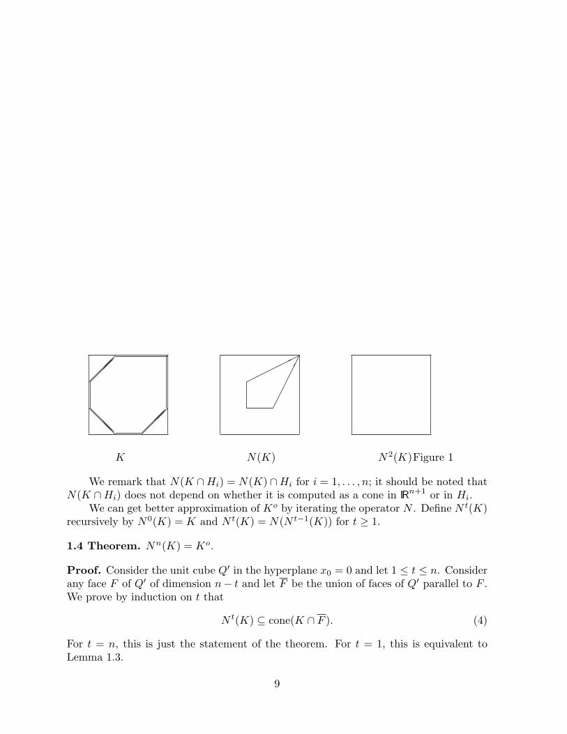
Figure 1 shows the intersection of three cones in IR3 with the hyperplane x3 = 1:the cones K, N(K) and N(N(K)), and the constraints implied by Lemma 1.3. We seethat the cone in Lemma 1.3 gets close to N(K) but does not conincide with it.

8

¡¡¡

¡¡¡

@@@

@@@ ¡

¡¡¡

¡¡¢¢¢¢¢

©©©©©

K N(K) N2(K)Figure 1

We remark that N(K ∩Hi) = N(K) ∩Hi for i = 1, . . . , n; it should be noted thatN(K ∩Hi) does not depend on whether it is computed as a cone in IRn+1 or in Hi.

We can get better approximation of Ko by iterating the operator N . Define N t(K)recursively by N0(K) = K and N t(K) = N(N t−1(K)) for t ≥ 1.

1.4 Theorem. Nn(K) = Ko.

Proof. Consider the unit cube Q′ in the hyperplane x0 = 0 and let 1 ≤ t ≤ n. Considerany face F of Q′ of dimension n− t and let F be the union of faces of Q′ parallel to F .We prove by induction on t that

N t(K) ⊆ cone(K ∩ F ). (4)

For t = n, this is just the statement of the theorem. For t = 1, this is equivalent toLemma 1.3.

9

We may assume that F contains the vector e0. Let F ′ be a (n− t + 1)-dimensionalface of Q′ containing F and i, an index such that F ′ ∩Hi = F . Then by the inductionhypothesis,

N t−1(K) ⊆ cone(K ∩ F ′).

Hence by Lemma 1.3,

N t(K) =N(N t−1(K)) ⊆ cone(N t−1(K) ∩ (Hi ∪Gi))

⊆cone([cone(K ∩ F ′) ∩Hi] ∪ [cone(K ∩ F ′) ∩Gi]).

Now Hi is a supporting plane of cone(K ∩ F ′) and hence its intersection with the coneis spanned by its intersection with the generating set of the cone:

cone(K ∩ F ′) ∩Hi = cone(K ∩ F ′ ∩Hi) ⊆ cone(K ∩ F ).

Similarly,

cone(K ∩ F ′) ∩Gi ⊆ cone(K ∩ F ).

Hence (4) follows.

Next we show that if we use positive semidefiniteness, i.e., we consider N+(K), thenan analogue of Lemma 1.3 can be obtained, which is more complicated but importantin the applications to combinatorial polyhedra.

1.5 Lemma. Let K ⊆ Q be a convex cone and let a ∈ IRn+1 be a vector such thatai ≤ 0 for i = 1, . . . , n and a0 ≥ 0. Assume that aT x ≥ 0 is valid for K ∩ Gi for all isuch that ai < 0. Then aT x ≥ 0 is valid for N+(K).

(The condition that a0 ≥ 0 excludes only trivial cases. The condition that ai ≤ 0is a normalization, which can be achieved by flipping coordinates.)

Proof. First, assume that a0 = 0. Consider a subscript i such that ai < 0. (If no such iexists, we have nothing to prove.) Then for every x ∈ Gi \{0}, we have aT x ≤ aixi < 0,and so, x /∈ K. Hence K ∩Gi = {0} and so by Lemma 1.3, N+(K) ⊆ N(K) ⊆ K ∩Hi.As this is true for all i with ai < 0, we know that aT x = 0 for all x ∈ N+(K).

Second, assume that a0 > 0. Let x ∈ N+(K) and let Y ∈ M+(K) be a ma-trix with Y e0 = x. For any 1 ≤ i ≤ n, the vector Y ei is in K by (iii”) andin Gi by (ii); so by the assumption on a, aT Y ei ≥ 0 whenever ai < 0. HenceaT Y (a0e0 − a) = aT Y (−a1e1 − . . . − anen) ≥ 0 (since those terms with ai = 0 donot contribute to the sum anyway), and hence aT Y (a0e0) ≥ aT Y a ≥ 0 by positivesemidefiniteness. Thus aT Y e0 = aT x ≥ 0.

10

c. Algorithmic aspects. Next we turn to some algorithmic aspects of these con-structions. We have to start by sketching the framework we are using; for a detaileddiscussion, see Grotschel, Lovasz and Schrijver (1988).

Let K be a convex cone. A strong separation oracle for the cone K is a subroutinethat, given a vector x ∈ CQn+1, either returns that x ∈ K or returns a vector w ∈ K∗

such that xT w < 0. A weak separation oracle is a version of this which allows fornumerical errors: its input is a vector x ∈ CQn and a rational number ε > 0, and iteither returns the assertion that the euclidean distance of x from K is at most ε, orreturns a vector w such that |w| ≥ 1, wT x ≤ ε and the euclidean distance of w from K∗

is at most ε. If the cone K is spanned by 0-1 vectors then we can strengthen a weakseparation oracle to a strong one in polynomial time.

Let us also recall the following consequence of the ellipsoid method: Given a weakseparation oracle for a convex body, together with some technical information (say, theknowledge of a ball contained in the body and of another one containing the body),we can optimize any linear objective function over the body in polynomial time (again,allowing an arbitrarily small error). If we have a weak separation oracle for a convexcone K ⊆ Q then we can consider its intersection with the half-space x0 ≤ 1; usingthe above result, we can solve various important algorithmic questions concerning K inpolynomial time. We mention here the weak separation problem for the polar cone K∗.

1.6 Theorem. Suppose that we have a weak separation oracle for K. Then the weakseparation problem for N(K) as well as for N+(K) can be solved in polynomial time.

Proof. Suppose that we have a (weak) separation oracle for the cone K. Then we havea polynomial time algorithm to solve the (weak) separation problem for the cone M(K).In fact, let Y be any matrix. If it violates (i) or (ii) then this is trivially recognizedand a separating hyperplane is also trivially given. (iii) can be checked as follows: wehave to know if Y u ∈ K holds for each u ∈ Q∗. Clearly it suffices to check this forthe extreme rays of Q∗, i.e. for the vectors ei and fi. But this can be done using theseparation oracle for K.

Since N(K) is a projection of K, the weak separation problem for N(K) can be alsosolved in polynomial time (by the general results from Grotschel, Lovasz and Schrijver1988).

In the case of N+(K), all we have to add that the positive semidefiniteness of thematrix Y can be checked by Gaussian elimination, pivoting always on diagonal entries.If we always pivot positive elements, the matrix is positive semidefinite. If the test fails,it is easy to construct a vector v with vT Y v < 0; this gives then a hyperplane separatingY from the cone.

We remark that this proof does not remain valid for N(K, K). In fact, let K bethe cone induced by the incidence vectors of perfect matchings of a graph G with mnodes (with “1” appended as a 0th entry). Then the separation problem for K can be

11

solved in polynomial time. On the other hand, consider the matrix Y = (Yij) where

yij ={

1, if i = j or i = 0 or j = 0,−4(m + 2)/m2, otherwise.

Then Y ∈ M(K, K) if and only if G is 3-edge-colorable, which is NP-complete todecide. We don’t know if theorem 1.6 extends to N(K, K), but suspect that the answeris negative.

Note, however, that if K is given by an explicit system of linear inequalities thenM(K,K) is described by a system of linear inequalities of polynomial size and so theseparation problem for N(K, K) and N+(K, K) can be solved in polynomial time. Inthis case, we get a projection representation of N(K) and of N(K, K) from polyhedrawith a polynomial number of facets. It should be remarked that this representation iscanonical.

d. Stronger cut operators. We could use stronger versions of this procedure to getconvex sets smaller than N(K).

One possibility is to consider N(K,K) instead of N(K) = N(K, Q). It is clearthat N(K,K) ⊆ N(K). Trivially, theorem 1.4, and lemma remain valid if we replaceN(K) by N(K,K). Unfortunately, it is not clear whether theorem 1.6 also remainsvalid. The problem is that now we have to check whether Y K∗ ⊆ K and unfortunatelyK∗ may have exponentially many, or even infinitely many, extreme rays. If K is givenby a system of linear inequalities then this is not a problem. So in this case we couldconsider the sequence N(K,K), N(N(K, K),K), etc. This shrinks down faster to Ko

than N t(K), as we shall see in the next section.The following strengthening of the projection step in the construction seems quite

interesting. For v ∈ IRn+1, let M(K)v = {Y v : Y ∈ M(K)}. So N(K) = M(K)e0.Now define

N(K) = ∩v∈int(Q∗)M(K)v.

Note that the intersection can be written in the form

N(K) = ∩u∈Q∗M(K)(e0 + u).

It is easy to see thatKo ⊆ N(K) ⊆ N(K).

The following lemma gives a different characterization of N(K):

1.7 Lemma. x ∈ N(K) if and only if for every w ∈ IRn+1 and every u ∈ Q∗ such that(e0 + u)wT ∈ M(K)∗, we have wT x ≥ 0.

In other words, N(K)∗ is generated by those vectors w for which there exists av ∈ int(Q∗) such that vwT ∈ M(K)∗.

Proof. (Necessity) Let x ∈ N(K), w ∈ IRn+1 and v ∈ int(Q∗) such that vwT ∈ M(K)∗.Then in particular x can be written as x = Y v where Y ∈ M(K). So wT x = wT Y v =Y · (vwT ) ≥ 0.

12

(Sufficiency) Assume that x /∈ N(K). Then there exists a v ∈ int(K∗) such thatx /∈ M(K)v. Now M(K)v is a convex cone, and hence it can be separated from x bya hyperplane, i.e., there exists a vector w ∈ IRn+1 such that wT x < 0 but wT Y v ≥ 0for all Y ∈ M(K). This latter condition means that vwT ∈ M(K)∗, i.e., the conditiongiven in the lemma is violated.

The cone N(K) satisfies important constraints that the cones N(K) and N+(K)do not. Let b ∈ IRn+1, and define Fb = {x ∈ IRn+1 : bT x ≥ 0}.

1.8 Lemma. Assume that N(K ∩ Fb) = {0}. Then −b ∈ N(K)∗.

Proof. If N(K ∩ Fb) = {0} then for every matrix Y ∈ M(K ∩ Fb) we have Y e0 = 0.In particular, Y00 = 0 and hence Y = 0. So M(K ∩ Fb) = {0}. Since clearly

M(K ∩ Fb)∗ = M(K)∗ + cone{buT : u ∈ Q∗},

this implies that M(K)∗ + {buT : u ∈ Q∗} = IR(n+1)×(n+1). So in particular we canwrite −beT

0 = Z + buT with Z ∈ M(K)∗ and u ∈ Q∗. Hence −b(e0 +u)T ∈ M(K)∗. Bythe previous lemma, this implies that −b ∈ N(K)∗.

We can use this lemma to derive a geometric condition on N(K) similar to Lemma1.5:

1.9 Lemma. Let K ⊆ Q be a convex cone and assume that e0 /∈ K. Then

N(K) ⊆ (K ∩G1) + . . . + (K ∩Gn).

In other words, if aT x ≥ 0 is valid for all of the faces K ∩ Gi then it is also validfor N(K).

Proof. Let b = −a + te0, where t > 0. Consider the cone K ∩ Fb. By the definition ofb, this cone does not meet any facet Gi of Q in any non-zero vector. Hence by Lemma1.3, N(K ∩ Fb) is contained in every facet Hi of Q, and hence N(K ∩ Fb) ⊆ cone(e0).But N(K ∩ Fb) ⊆ K and so N(K ∩ Fb) = {0}.

Hence by Lemma 1.7, we get that −b = a− te0 ∈ N(K)∗. Since this holds for everyt < α and N(K)∗ is closed, the lemma follows.

Applying this lemma to the cone in Figure 1, we can see that we obtain Ko in asingle step. The next corollary of Lemma 1.9 implies that at least some of the Gomory–Chvatal cuts for K are satisfied by N(K):

1.10 Corollary. Let 1 ≤ k ≤ n and assume that∑k

i=1 xi > 0 holds for every x ∈ K.Then

∑ki=1 xi ≥ x0 holds for every x ∈ N(K).

13

The proof consists of applying Lemma 1.9 to the projection of K on the first k + 1coordinates.

Unfortunately, we do not know if Theorem 1.6 remains valid for N(K). Of course,the same type of projection can be defined starting with M+(K) or with M(K, K)instead of M(K), and properties analogous to those in Lemmas 1.8–1.9 can be derived.

14

2. Stable set polyhedra

We apply the results in the previous section to the stable set problem. To this end,we first survey some known methods and results on the facets of stable set polytopes.

a. Facets of stable set polyhedra and perfect graphs. Let G = (V, E) be a graphwith no isolated nodes. Let α(G) denote the maximum size of any stable set of nodesin G. For each A ⊆ V , let χA ∈ IRV denote its incidence vector. The stable set polytopeof G is defined as

STAB(G) = conv{χA : A is stable}.So the vertices of STAB(G) are just the 0-1 solutions of the system of linear inequalities

xi ≥ 0 for each i ∈ V, (1)

andxi + xj ≤ 1 for each ij ∈ E. (2)

In general, STAB(G) is much smaller than the solution set of (1)–(2), which wedenote by FRAC(G) (“fractional stable sets”). In fact, they are equal if and only ifthe graph is bipartite. The polytope FRAC(G) has many nice properties; what we willneed is that its vertices are half-integral vectors.

There are several classes of inequalities that are satisfied by STAB(G) but notnecessarily by FRAC(G). Let us mention some of the most important classes. Theclique constraints strengthen the class (2): for each clique B, we have

∑

i∈B

xi ≤ 1. (3)

Graphs for which (1) and (3) are sufficient to describe STAB(G) are called perfect.It was shown by Grotschel, Lovasz and Schrijver (1981) that the weighted stable setproblem can be solved in polynomial time for these graphs.

The odd hole constraints express the non-bipartiteness of the graph: if C induces achordless odd cycle in G then

∑

i∈C

xi ≤ 12(|C| − 1). (4)

Of course, the same inequality holds if C has chords; but in this case it easily followsfrom other odd hole constraints and edge constraints. Nevertheless, it will be convenientthat if we apply an odd hole constraint, we do not have to check whether the circuit inquestion is chordless.

15

Graphs for which (1), (2) and (4) are sufficient to describe STAB(G) are calledt-perfect. Graphs for which (1), (3) and (4) are sufficient are called h-perfect. It wasshown by Grotschel, Lovasz and Schrijver (1986) that the weighted stable set problemcan be solved in polynomial time for h-perfect (and hence also for t-perfect) graphs.

The odd antihole constraints are defined by sets D that induce a chordless odd cyclein the complement of G: ∑

i∈D

xi ≤ 2. (5)

We shall see that the the weighted stable set problem can be solved in polynomial timefor all graphs for which (1)–(5) are enough to describe STAB(G) (and for many moregraphs).

All constraints (2)–(5) are special cases of the rank constraints: let U ⊆ V inducea subgraph GU , then ∑

i∈U

xi ≤ α(GU ). (6)

Of course, many of these constraints are inessential. To specify some that are essential,let us call a graph G α-critical if it has no isolated nodes and α(G−e) > α(G) for everyedge e. Chvatal (1975) showed that if G is a connected α-critical graph then the rankconstraint ∑

i∈V (G)

xi ≤ α(G)

defines a facet of STAB(G).(Of course, in this generality rank constraints are ill-behaved: given any one of

them, we have no polynomial time procedure to verify that it is indeed a rank constraint,since we have no polynomial time algorithm to compute the stability number of thegraph on the right hand side. For the special classes of rank constraints introducedabove, however, it is easy to verify that a given inequality belongs to them.)

Finally, we remark that not all facets of the stable set polytope are determined byrank constraints. For example, let U induce an odd wheel in G, with center u0 ∈ U .Then the constraint ∑

i∈U\{u0}xi +

|U | − 22

xu0 ≤|U | − 2

2

is called a wheel constraint. If e.g. V (G) = U then the wheel constraint induces a facetof the stable set polytope.

Another class of non-rank constraints of a rather different character are orthogonal-ity constraints, introduced by Grotschel, Lovasz and Schrijver (1986). Let us associatewith each vertex i ∈ V , a vector vi ∈ IRn, so that |vi| = 1 and non-adjacent verticescorrespond to orthogonal vectors. Let c ∈ IRn with |c| = 1. Then

∑

i∈V

(cT vi)2xi ≤ 1

16

is valid for STAB(G). The solution set of these constraints (together with the non-negativity constraints) is denoted by TH(G). It is easy to show that

STAB(G) ⊆ TH(G) ⊆ FRAC(G).

In fact, STAB(G) satisfies all the clique constraints. Note that there are infinitely manyorthogonality constraints for a given graph, and TH(G) is in general non-polyhedral (itis polyhedral if and only if the graph is perfect). The advantage of TH(G) is that everylinear objective function can be optimized over it in polynomial time. The algorithminvolves convex optimization in the space of matrices, and was the main motivation forour studies in the previous section. We shall see that these techniques give substantiallybetter approximations of STAB(G) over which one can still optimize in polynomial time.

b. The “N” operator.” To apply the results in the previous chapter, we homogenizethe problem by introducing a new variable x0 and consider STAB(G) as a subset of thehyperplane H0 defined by x0 = 1. We denote by ST(G) the cone spanned by the vectors(

1χA

) ∈ IRV ∪{0}, where A is a stable set. We get STAB(G) by intersecting ST(G) withthe hyperplane x0 = 1. Similarly, let FR(G) denote the cone spanned by the vectors(1x

)where x ∈ FRAC(G). Then FR(G) is determined by the constraints

xi ≥ 0 for each i ∈ V,

andxi + xj ≤ x0 for each ij ∈ E.

Since it is often easier to work in the original n-dimensional space (without homog-enization), we shall use the notation N(FRAC(G)) = N(FR(G))∩H0 and similarly forN+, N etc. We shall also abbreviate N(FRAC(G)) by N(G) etc. Since FRAC(G) isdefined by an explicit linear program, one can solve the separation problem for it inpolynomial time. We shall say briefly that the polytope is polynomial time separable.By Theorem 1.6, we obtain the following.

2.1 Theorem. For each fixed r ≥ 0, Nr+(G) as well as Nr(G) are polynomial time

separable.

It should be remarked that, in most cases, if we use Nr(G) as a relaxation ofSTAB(G) then it does not really matter whether the separation subroutine returnshyperplanes separating the given x /∈ Nr(G) from Nr(G) or only from STAB(G). Henceit is seldom relevant to have a separation subroutine for a given relaxation, say Nr(G);one could use just as well a separation subroutine for any other convex body containingSTAB(G) and contained in Nr(G) (such as e.g. Nr

+(G)). Hence the polynomial timeseparability of Nr

+(G) is substantially deeper than the polynomial time separability ofNr(G) (even though it does not imply it directly).

In the rest of this section we study the question of how much this theorem givesus: which graphs satisfy Nr

+(G) = STAB(G) for small values of r, and more generally,

17

which of the known constraints are satisfied by N(G), N+(G), etc. With a little abuseof terminology, we shall not distinguish between the original and homogenized versionsof clique, odd hole, etc. constraints.

It is a useful observation that if Y = (yij) ∈ M(FR(G)) then yij = 0 wheneverij ∈ E(G). In fact the constraint xi +xj ≤ 1 must be satisfied by Y ei, and so yii +yji ≤y0i = yii by non-negativity. This implies yij = 0.

Let aT x ≤ b be any inequality valid for STAB(G). Let W ⊆ V and let aW ∈ IRW bethe restriction of a to W . For every v ∈ V , if aT x ≤ b is valid for STAB(G) then aT

V−vx ≤b is valid for STAB(G− v) and aT

V−Γ(v)−vx ≤ b − av is valid for STAB(G − Γ(v) − v).Let us say that these inequalities arise from aT x ≤ b by the deletion and contraction ofnode v, respectively. Note that if aT x ≤ b is an inequality such that for some v, boththe deletion and contraction of v yield inequalities valid for the corresponding graphs,then aT x ≤ b is valid for G.

Let K be any convex body containing STAB(G) and contained in FRAC(G). NowLemma 1.3 implies:

2.2 Lemma If aT x ≤ b is an inequality valid for STAB(G) such that for some v ∈ V ,both the deletion and contraction of v gives an inequality valid for K then aT x ≤ b isvalid for N(G).

This lemma enables us to completely characterize the constraints obtained in onestep (not using positive semidefiniteness):

2.3 Theorem The polytope N(G) is exactly the solution set of the non-negativity, edge,and odd hole constraints.

Proof. 1. It is obvious that N(G) satisfies the non-negativity and edge constraints.Consider an odd hole constraint

∑i∈C xi ≤ 1

2 (|C| − 1). Then for any i ∈ C, both thecontraction and deletion of i results in an inequality trivially valid for FRAC(G). Hencethe odd hole constraint is valid for N(G) by Lemma 2.2.

2. Conversely, assume that x ∈ IRV satisfies the non-negativity, edge-, and oddhole constraints. We want to show that there exists a non-negative symmetric matrixY = (yij) ∈ IR(n+1)×(n+1) such that yi0 = yii = xi for all 1 ≤ i ≤ n, y00 = 1, and

xi + xj + xk − 1 ≤ yik + yjk ≤ xk

for all i, j, k ∈ V such that ij ∈ E (the lower bound comes from the condition thatY fk ∈ FR(G), the upper, from the condition that Y ek ∈ FR(G)). Note that theconstraint has to hold in particular when i = k; then the upper bound implies thatyij = 0, while the lower bound is automatically satisfied.

The constraints on the y’s are of a special form: they only involve two variables.So we can use the following (folklore) lemma, which gives a criterion for the solvabilityof such a system, more combinatorial than the Farkas Lemma:

18

2.4 Lemma. Let H = (W,F ) be a graph and let two values 0 ≤ a(ij) ≤ b(ij) beassociated with each edge of H. Let U ⊆ W be also given. Then the linear system

a(ij) ≤ yi + yj ≤ b(ij), (ij ∈ F )

yi ≥ 0 (i ∈ W ),

yi = 0 (i ∈ U)

has no solution if and only if there exists a sequence of (not necessarily distinct) verticesv0, v1, . . . , vp such that vi and vi+1 are adjacent (the sequence is a walk), and one of thefollowing holds:

a) p is odd and b(v0v1)− a(v1v2) + b(v2v3)− . . . + b(vp−1vp) < 0;b) p is even, v0 = vp, and b(v0v1)− a(v1v2) + b(v2v3)− . . .− a(vp−1vp) < 0;c) p is even, vp ∈ U , and b(v0v1)− a(v1v2) + b(v2v3)− . . .− a(vp−1vp) < 0;d) p is odd, v0, vp ∈ U , and −a(v0v1) + b(v1v2)− a(v2v3)− . . .− a(vp−1vp) < 0.

In our case, we have as W the set of all pairs {i, j} (i 6= j), U is the subsetconsisting of the edges of G, two pairs are adjacent in H iff they intersect, and a(ij, jk) =xi + xj + xk − 1, b(ij, jk) = xj . We want to verify that if x satisfies all the odd holeconstraints then none of the walks of the type a)–d) in the lemma above can occur.Let us ignore for a while how the walk ends. The vertices of the walk in H correspondto pairs ij; the edges in the walk correspond to triples (ijk) such that ik ∈ E. Letus call this edge the bracing edge of the triple. We have to add up alternately xj and1− xi − xj − xk; call the triple positive and negative accordingly.

Let w be a vertex of G that is not an element of the first and last pair v0 and vp.Then following the walk, w may become an element of a vi, stay an element for a while,and the cease to be; this may be repeated, say, f(w) times. It is then easy to see thatthe total contribution of the variable xw to the sum is −f(w)xw.

It is easy to settle case b) now. Then any vi can be considered first, and so theabove counting applies to each vertex (unless all pairs vi share a vertex of G, which isa trivial case). So the sum

b(v0v1)− a(v1v2) + b(v2v3)− . . .− a(vp−1vp) =p

2−

∑w

f(w)xw.

But note that every vertex w occurs in exactly 2f(w) bracing edges. If we add up theedge constraints for all bracing edges, we get p −∑

w 2f(w)xw ≥ 0, which shows thatb) cannot occur.

Cases a) and c) only take a little care around the end of the walk, and are left tothe reader. Let us show how case d) can be settled, which is the only case when theodd hole constraints are needed.

Consider again the bracing edges of the triples, except that count now the pairsv0 and vp (which are edges of G) as bracing edges. Again, it is easy to see that thetotal sum in question is (p + 1)/2 − ∑

f(w)xw, where each w is contained in exactly

19

2f(w) bracing edges. Unfortunately, we now have p+2 bracing edges, so adding up theedge constraints for them would not yield the non-negativity of the sum. But observethat the multiset of bracing edges (we count an edge that is bracing in more than onetriple with multiplicity) forms an Eulerian graph, and is, therefore, the union of circuits.Since the total number of bracing edges, p + 2, is odd, at least one of these circuits isodd. Add up the odd hole constraint for this circuit and the edge constraint, dividedby two, for each of the remaining bracing edges. We get that

∑w f(w)xw ≤ (p + 1)/2,

which shows that d) cannot occur.

2.5 Corollary. If G is t-perfect then STAB(G) is the projection of a polytope whosenumber of facets is polynomial in n. Moreover, this representation is canonical.

This Corollary generalizes a result of Barahona and Mahjoub (1987) that constructsa projection representation for series-parallel graphs. It could also be derived in analternative way. The separation problem for the odd cycle inequalities can be reducedto n shortest path problems (see Grotschel, Lovasz and Schrijver 1986). Following thisconstruction, one can see that a vector x is in the stable set polytope of a t-perfectgraph if and only if n potential functions exist in an auxiliary graph. This yields arepresentation of STAB(G) as the projection of a polytope with O(n2) facets. (We aregrateful to the referee for this remark.)

c. The repeated “N” operator. Next we prove a theorem which describes a largeclass of inequalities valid for Nr(G) for a given r. The result is not as complete as inthe case r = 1, but it does show that the number of constraints obtainable grows veryquickly with r.

Let aT x ≤ b be any inequality valid for STAB(G). By Theorem 1.4, there exists anr ≥ 0 such that aT x ≤ b is valid for Nr(G). Let the N -index of the inequality be definedas the least r for which this is true. We can define (and will study later) the N+-indexanalogously. Note that in each version, the index of an inequality depends only on thesubgraph induced by those nodes having a non-zero coefficient. In particular, if thesenodes induce a bipartite graph then the inequality has N -index 0. We can define theN -index of a graph as the largest N -index of the facets of STAB(G). The N -index ofG is 0 if and only if G is bipartite; the N -index of G is 1 if and only if G is t-perfect.Lemma 2.2 implies (using the obvious fact that the N -index of an induced subgraph isnever larger than the N -index of the whole graph):

2.6 Corollary. If for some node v, G− v has N -index k then G has N -index at mostk + 1.

The following lemma about the iteration of the operator N will be useful in esti-mating the N -index of a constraint.

2.7 Lemma. 1k+21I. ∈ Nk(G) (k ≥ 0).

20

Proof. We use induction on k. The case k = 0 is trivial. Consider the matrix Y =(yij) ∈ IR(V ∪{0})×(V ∪{0}) defined by

yij =

1, if i = j = 0,1

k+1 , if i = 0 and j > 0, or i > 0 and j = 0,or i = j > 0,

0, otherwise.

Then Y ∈ M(Nk−1(FR(G))

), since

Y ei =1

k + 2(e0 + ei) ∈ ST(G) ⊆ Nk−1(FR(G))

and

Y fi =k + 1k + 2

e0 +∑

j 6=0,i

1k + 2

ej ≤ k + 1k + 2

e0 +

1k + 1

∑

j∈V

ej

∈ Nk−1(FR(G))

and so by the monotonicity of Nk−1(FR(G)), Y fi ∈ Nk−1(FR(G)). Hence the firstcolumn of Y is in Nk(FR(G)), and thus 1

k+21I. ∈ Nk(G).

From these two facts, we can derive some useful bounds on the N -index of a graph.

2.8 Corollary. Let G be a graph with n nodes and at least one edge. Assume that Ghas stability number α(G) = α and N -index k. Then

n

α− 2 ≤ k ≤ n− α− 1.

Proof. The upper bound follows from Corollary 2.6, applying it repeatedly to allbut one nodes outside a maximum stable set. To show the lower bound, assume thatk < (n/α) − 2. Then the vector 1

k+21I. does not satisfy the constraint∑

i xi ≤ α andso it does not belong to STAB(G). Since it belongs to Nk(G) by Lemma 2.7, it followsthat Nk(G) 6= STAB(G), a contradiction.

It follows in particular that the N -index of a complete graph on t vertices is t− 2.The N -index of an odd hole is 1, as an odd whole is a t-perfect graph. The N -index ofan odd antihole with 2k + 1 nodes is k; more generally, we have the following corollary:

2.9 Corollary. The N -index of a perfect graph G is ω(G) − 2. The N -index of acritically imperfect graph G is ω(G)− 1.

21

Next we study the index of a single inequality. Let aT x ≤ b be any constraint validfor STAB(G) (a ∈ ZZV

+, b ∈ ZZ+). Define the defect of this inequality as 2 ·max{aT − b :x ∈ FRAC(G)}. The factor 2 in front guarantees that this is an integer. In the specialcase when we consider the constraint

∑i xi ≤ α(G) for an α-critical graph G, the defect

is just the Gallai class number of the graph (see Lovasz and Plummer (1986) for adiscussion of α-critical graphs, in particular of the Gallai class number).

Given a constraint, its defect can be computed in polynomial time, since optimizingover FRAC(G) is an explicit linear program. The defect of a constraint is particularlyeasy to compute if the constraint defines a facet of STAB(G). This is shown by thefollowing lemma, which states a property of facets of STAB(G) of independent interest.

2.10 Lemma. Let∑

i aixi ≤ b define a facet of STAB(G), different from those deter-mined by the non-negativity and edge constraints. Then every vector v maximizing aT xover FRAC(G) has vi = 1/2 whenever ai > 0. In particular,

max{aT x : x ∈ FRAC(G)} =12

∑

i

ai

and the defect of the inequality is∑

i ai − 2b.

Proof. Let v be any vertex of FRAC(G) maximizing aT x. It suffices to prove thatvi 6= 1 whenever ai > 0; this will imply that the vector (1/2, . . . , 1/2)T also maximizesaT x, and to achieve the same objective value, v must have vi = 1/2 whenever ai > 0.

Let U = {i ∈ V : vi = 1} and assume, by way of contradiction, that a(U) > 0.Clearly U is a stable set. If we choose v so that U is minimal (but of course non-empty),then ai > 0 for every i ∈ U . Let Γ(U) denote the set of neighbors of U . Let X beany stable set in G whose incidence vector χX is a vertex on the facet of STAB(G)determined by aT x = b.

Consider the set Y = U ∪ (X \Γ(U)). Clearly, Y is stable and a(Y ) = a(X)+a(U \X)− a(Γ(U) ∩X). So by the optimality of X, we have

a(U \X) ≤ a(Γ(U) ∩X).

On the other hand, consider the vector w ∈ IRV defined by

wi =

1, if i ∈ U ∩X,0, if i ∈ Γ(U) \X,12 , otherwise.

Then w ∈ FRAC(G) and aT w ≥ aT v + (1/2)a(Γ(U) ∩X)− (1/2)a(U \X) ≥ aT v. Bythe optimality of v, we must have equality, and so a(U \X) = a(Γ(U) ∩X). But thismeans that χX satisfies the linear equation

∑

i∈U∪Γ(U)

aixi = a(U).

22

So this linear equation is satisfied by every vertex of the facet determined by aT x = b.The only way this can happen is that it is the equation aT x = b itself. But then aT v = band so aT v ≤ b defines also a facet of FRAC(G), which was excluded.

We need some further, related lemmas about stable set polytopes. These may beviewed as weighted versions of results on graphs with the so-called Konig property; seeLovasz and Plummer (1986), section 6.3.

2.11 Lemma. Let a ∈ IRV+ and assume that

max{aT x : x ∈ STAB(G)} < max{aT x : x ∈ FRAC(G)}.

Let E′ be the set of those edges ij for which yi + yj = 1 holds for every vector y ∈FRAC(G) maximizing aT x. Then (V, E′) is non-bipartite.

Proof. Suppose that (V, E′) is bipartite. Let z be a vector in the relative interior ofthe face F of FRAC(G) maximizing aT x. Then clearly

E′ = {ij ∈ E : zi + zj = 1}

andF = {x ∈ FRAC(G) : xi + xj = 1 for all ij ∈ E}.

Let (U,W ) be a bipartition of (V, E′). In every connected component of (V, E′), zi ≥ 1/2on at least one color class and hence we may choose (U,W ) so that zi ≥ 1/2 for alli ∈ W . Then W is a stable set in the whole graph G. Hence it follows that χW ∈ F .This implies that max{aT x : x ∈ STAB(G)} = max{aT x : x ∈ FRAC(G)}, a contra-diction.

2.12 Lemma. As in the previous lemma, let a ∈ IRV+ and assume that

max{aT x : x ∈ STAB(G)} < max{aT x : x ∈ FRAC(G)}.

Then there exists an i ∈ V such that every vector y ∈ FRAC(G) maximizing aT x hasyi = 1/2.

Proof. Let E′ be as before. Then by Lemma 2.11, there exists an odd circuit C in Gsuch that E(C) ⊆ E′. If y is any vector in FRAC(G) maximizing aT x then by the defini-tion of E′, yi +yj = 1 for every edge ij ∈ E(C), and hence yi = 1/2 for every i ∈ V (C).

Now we can state and prove our theorem that shows the connection between defectand the N -index:

23

2.13 Theorem. Let aT x ≤ b be an inequality with integer coefficients valid forSTAB(G) with defect r and N -index k. Then

r

b≤ k ≤ r.

Proof. (Upper bound.) We use induction on r. If r = 0 we have nothing to prove,so suppose that r > 0. Then Lemma 2.12 can be applied and we get that there is avertex i such that every vector y optimizing aT x over FRAC(G) has yi = 1/2. Notethat trivially ai > 0.

We claim that both the contraction and deletion of i result in constraints withsmaller defect. In fact, let y be a vertex of FRAC(G) maximizing aT

V−ix. If y alsomaximizes aT x then yi = 1/2 and hence

2(aTV−iy − b) = 2(aT y − b)− ai < 2(aT y − b) = r.

On the other hand, if y does not maximize aT x then

2(aTV−iy − b) ≤ 2(aT y − b) < 2 ·max{aT x− b : x ∈ FRAC(G)} = r.

The assertion follows similarly for the contraction. Hence by the induction hypothesis,the contraction and deletion of i yields constraints valid for Nr−1(G). It follows byLemma 2.2 that aT x ≤ b is valid for Nr(G).

(Lower bound.) By Lemma 2.7, 1k+21I. ∈ Nk(G), and so aT x ≤ b must be valid for

1k+21I.. So 1

k+2aT 1I. ≤ b and hence

k ≥ aT 1I.

b− 2 =

r

b.

It follows from our discussions that for an odd antihole constraint, the lower boundis tight. On the other hand, it is not difficult to check that for a rank constraint definedby an α-critical subgraph that arises from Kp by subdividing an edge by an even numberof nodes, the upper bound is tight.

We would like to mention that Ceria (1989) proved that N(FRAC(G), FRAC(G))also satisfies, among others, the K4-constraints. We do not study the operator K 7→N(K,K) here in detail, but a thorough comparison of its strength with N and N+

would be very interesting.A class of graphs interesting from the point of view of stable sets is the class of line-

graphs: the stable set problem for these graphs is equivalent to the matching problem.In particular, it is polynomial time solvable and Edmonds’ description of the matchingpolytope (Edmonds 1965) provides a “nice” system of linear inequalities describing thestable set polytope of such graphs. The N -index of line-graphs is unbounded; this

24

follows e.g. by Corollary 2.8. This also follows from Yannakakis’ result mentioned inthe introduction, since bounded N -index would yield a representation of the matchingpolytope as a projection of a polytope with a polynomial number of facets. We do notknow whether or not the N+-index of line-graphs remains bounded.

d. The “N+” operator. Now we turn to the study of the operator N+ for stable setpolytopes. We do not have as general results as for the operator N , but we will be ableto show that many constraints are satisfied even for very small r.

Lemma 2.3 implies:

2.14 Lemma. If aT x ≤ b is an inequality valid for STAB(G) such that for all v ∈ Vwith a positive coefficient the contraction of v gives an inequality with N+-index at mostr, then aT x ≤ b has N+-index at most r + 1.

The clique, odd hole, odd wheel, and odd antihole constraints have the propertythat contracting any node with a positive coefficient we get an inequality in which thenodes with positive coefficients induce a bipartite subgraph. Hence

2.15 Corollary. Clique, odd hole, odd wheel, and odd antihole constraints have N+-index 1.

Hence all h-perfect (in particular all perfect and t-perfect) graphs have N+-indexat most 1. We can also formulate the following recursive upper bound on the N+-indexof a graph:

2.16 Corollary. If G− Γ(v) − v has N+-index at most r for every v ∈ V then G hasN+-index at most r + 1.

Next, we consider the orthogonality constraints. To this end, consider the coneMTH of (V ∪ {0})× (V ∪ {0}) matrices Y = (yij) satisfying the following constraints:

(i) Y is symmetric;

(ii) yii = yi0 for every i ∈ V ;

(iii’) yij = 0 for every ij ∈ E;

(iv) Y is positive semidefinite.

As remarked, (iii’) is a relaxation of (iii) in the definition of M+(FR(G)). HenceM+(FR(G)) ⊆ MTH .

2.17 Lemma. TH(G) = {Y e0 : Y ∈ MTH , eT0 Y e0 = 1}.

Proof. Let x ∈ TH(G). Then by the results of Grotschel, Lovasz and Schrijver (1986),x can be written in the form xi = (vT

0 vi)2, where the vi (i ∈ V ) form an orthonormalrepresentation of the complement of G and v0 is some vector of unit length. Set x0 = 1

25

and define Yij = vTi vj

√xixj . Then it is easy to verify that Y ∈ MTH and Y e0 = x.

The converse inclusion follows by a similar direct construction.

This representation of TH(G) is not a special case of the matrix cuts introducedin section 1 (though clearly related). In section 3 we will see that in fact TH(G) is ina sense more fundamental than the relaxations of STAB(G) constructed in section 1.Right now we can infer the following.

2.18 Corollary. Orthogonality constraints have N+-index 1.

We conclude with an upper bound on the N+-index of a single inequality. Sinceα(G− Γ(v)− v) < α(G), Lemma 2.3 gives by induction

2.19 Corollary. If aT x ≤ b is an inequality valid for STAB(G) such that the nodeswith positive coefficient induce a graph with independence number r then aT x ≤ b hasN+-index at most r. In particular, aT x ≤ b has index at most b.

Let us turn to the algorithmic aspects of these results. Theorem 2.1 implies:

2.20 Corollary. The maximum weight stable set problem is polynomial time solvablefor graphs with bounded N+-index.

Note that even for small values of r, quite a few graphs have N+-index at most r.Collecting previous results, we obtain:

2.21 Corollary. For any fixed r ≥ 0, if STAB(G) can be defined by constraints aT x ≤ bsuch that either the defect of the constraint is at most r or the support of a contains nostable set larger than r, then the maximum weight stable set problem is polynomial timesolvable for G.

26

3. Cones of set-functions

Vectors in IRS are just functions defined on the one-element subsets of a set S; thesymmetric matrices in the previous sections can be considered as functions defined onunordered pairs. We show that if we consider set-functions, i.e., functions defined onall subsets of S, then some of the previous considerations become more general andsometimes even simpler.

In fact, most of the results extend to a general finite lattice in the place of theBoolean algebra, and we present them in this generality for the sake of possible otherapplications.

a. Preliminaries: vectors on lattices. Let us start with some general facts aboutfunctions defined on lattices. Given a lattice L, we associate with it the matrix Z = (ζij),called the zeta-matrix of the lattice, defined by

ζij ={

1, if i ≤ j,0, otherwise.

For j ∈ L, let ζj denote the jth column of the zeta matrix, i.e., let

ζj(i) = ζij .

If we order the rows and columns of Z compatibly with the partial ordering definedby the lattice, it will be upper triangular with 1’s in its main diagonal. Hence it isinvertible, and its inverse M = Z−1 is an integral matrix of the same shape. Thisinverse is a very important matrix, called the Mobius matrix of the lattice. Let

M = (µ(i, j))i,j∈L.

The function µ is called the Mobius function of the lattice. From the discussion abovewe see that µ(i, i) = 1 for all i ∈ L, and µ(i, j) = 0 for all i, j ∈ L such that i 6≤ j.Moreover, the definition of M implies that for every pair of elements a ≤ b of the lattice,

∑

a≤i≤b

µ(a, i) ={

1, if a = b,0, otherwise;

and ∑

a≤i≤b

µ(i, b) ={

1, if a = b,0, otherwise.

Either one of these identities provides a recursive procedure to compute the Mobiusfunction. It is easy to see from this procedure that the value of the Mobius function

27

µ(i, j), where i ≤ j, depends only on the internal structure of the interval [i, j]. Alsonote the symmetry in these two identities. This implies that if µ∗ denotes the Mobiusfunction of the lattice turned upside down, then

µ∗(i, j) = µ(j, i).

For j ∈ L, let µj denote the jth column of the Mobius matrix, i.e., let

µj(i) = µij .

We denote by µj the jth row of the Mobius matrix, and by µ[i,j] the restriction of µitto the interval [i, j], i.e., vector defined by

µ[i,j](k) ={

µ(i, k), if k ≤ j,0, otherwise.

The Mobius function of a lattice generalizes the Mobius function in number theory,and it can be used to formulate an inversion formula extending the Mobius inversion innumber theory. Let g ∈ IRL be a function defined on the lattice. The zeta matrix canbe used to express its lower and upper summation function:

(ZT g)(i) =∑

j≤i

g(j),

and(Zg)(i) =

∑

j≥i

g(j).

Given (say) f = Zg, we can recover g uniquely by

g(i) = (Mf)(i) =∑

j≥i

µ(i, j)f(j).

The function g is called the upper Mobius inverse of f . The lower Mobius inverse isdefined analogously.

There is a further simple but important formula relating a function to its inverse.Given a function f ∈ IRL, we associate with it the matrix W f = (wij), where

wij = f(i ∨ j).

We also consider the diagonal matrix Df with (Df )ii = f(i). Then it is not difficult toprove the following identity (Lindstrom 1969, Wilf 1968):

3.1 Lemma. If g is the upper Mobius inverse of f then W f = ZDgZT .

28

For more on Mobius functions see Rota (1964), Lovasz (1979, Chapter 2), or Stanley(1986, Chapter 3).

A function f ∈ IRL will be called strongly decreasing if Mf ≥ 0. Since f = Z(Mf),this is equivalent to saying that f is a non-negative linear combination of the columns ofZ, i.e., of the vectors ζj . So strongly decreasing functions form a convex cone H = H(L),which is generated by the vectors ζj , j ∈ L. Also by definition, the polar cone H∗ isgenerated by the rows of M , i.e., by the vectors µj .

Let us mention that the vector µ[i,j] is also if H∗ for every i ≤ j. This is straightfor-ward to check by calculating the inner product of µ[i,j] with the generators ζj of H. Itis easy to see that strongly decreasing functions are non-negative, monotone decreasingand supermodular, i.e., they satisfy

f(i ∨ j) + f(i ∧ j) ≥ f(i) + f(j).

Lemma 3.1 implies:

Corollary 3.2 A function f is strongly decreasing if and only if W f is positive semidef-inite.

It follows in particular that f is strongly decreasing iff for every x ∈ IRL,

xT W fx =∑

i,j

xixjf(i ∨ j) ≥ 0.

It is in fact worth while to mention the following identity, following immediately fromLemma 3.1. Let f, x ∈ IRL and let g = Mf and y = Zx. Then

xT W fx =∑

i∈L

g(i)y(i)2.

In particular, if f is strongly decreasing then

xT W fx ≥ g(0)x(0)2. (5)

Remark. Let L = 2S , and let f ∈ IRL such that f(∅) = 1. Then f is strongly decreasingif and only if there exist random events As (s ∈ S) such that for every X ⊆ S,

Prob

( ∏

s∈X

As

)= f(X).

(If this is the case, (Mf)(X) is the probability of the atom∏

s∈X As

∏s∈S−X As.) In

particular, we obtain from (5) that for any λ ∈ IRL with λ(0) = 1,

∑

X,Y

λXλY Prob

( ∏

s∈X∪Y

As

)≥ Prob

(∏

i∈S

Ai

).

29

This is a combinatorial version of the Selberg Sieve in number theory (see Lovasz (1979),Chapter 2). Inequality (5) can be viewed as Selberg’s Sieve for general lattices; seeWilson (1970).

The lattice structure also induces a “multiplication”, which leads to the semigroupalgebra of the semigroup (L,∨). Given a, b ∈ IRL, we define the vector a ∨ b ∈ IRL by

(a ∨ b)(k) =∑

i∨j=k

a(i)b(j).

In particular,ei ∨ ej = ei∨j

(and the rest of the definition is obtained by distributivity). It is straightforward tosee that this operation is commutative, associative and distributive with respect to thevector addition, and has unit element e0 (where 0 is the zero element of the lattice).This semigroup algebra has a very simple structure: elementary calculations show that

ZT (a ∨ b)(k) = (ZT a)(k) · (ZT b)(k), (6)

and hence the semigroup algebra is isomorphic to the direct product of |L| copies of IR.It also follows from (6) that a vector a has an inverse in this algebra iff (ZT a)(k) 6= 0for all k.

Another identity which will be useful is the following:

(a ∨ b)T c = aT W cb. (7)

Using this, we can express the fact that a vector c is strongly decreasing as follows:

(a ∨ a)T c ≥ 0 for every a ∈ IRL.

In particular it follows that H∗ is generated by the vectors a ∨ a, a ∈ IRL. Comparingthis with our previous characterization it follows that the vectors µj must be of the forma∨a. In fact, µj ∨µj = µj ; more generally, the vectors µ[i,j] are also idempotent. Using(6) it is easy to see that the idempotents are exactly the vectors of the form

∑i∈I µi,

where I ⊆ L. Moreover, the “∨” product of any two vectors µi is zero.

b. Optimization in lattices. Given a subset F ⊆ L, we denote by cone(F ) theconvex cone spanned by the vectors ζi, i ∈ F . Since these vectors are extreme raysof H, and all extreme rays of H are linearly independent, it is in principle trivial todescribe F by linear inequalities: It is determined by the system

µTj x

{= 0, if i /∈ F ,≥ 0, if i ∈ F .

(8)

But since cone(F ) is in general not full-dimensional, it may have many other minimaldescriptions. For example, in the case when F is an order ideal (i.e., x ∈ F , y ≤ x implyy ∈ F ), cone(F ) could be described by

x ∈ H, x(i) = 0 for all i /∈ F. (9)

30

Hencecone(F )∗ = {a ∈ IRL : (ZT a)(k) ≥ 0 for all k ∈ F}. (10)

Our main concern will be to describe the projection of cone(F ) on the subspacespanned by a few “small” elements in the lattice. Let I be the set of these “interesting”lattice elements. We consider IRI as the subspace of IRL spanned by the elements of I.For any convex cone K ⊆ H, let KI denote the intersection of K with IRI and let K/Idenote the projection of K onto IRI . Then (K∗)I ⊆ K∗ is the set of linear inequalitiesvalid for K involving only variables corresponding to elements of I. Also, (K∗)I is thepolar of K/I with respect to the linear space IRI .

For example in the case when L = 2S , where S is an n-element set, we can take Ias the set of all singletons and ∅. If we project cone(F ) on this subspace, and intersectthe projection with the hyperplane x∅ = 1, then we recover the polyhedron usuallyassociated with F (namely the convex hull of incidence vectors of members of F ). Notethat the projection itself is just the homogenization introduced in the section 1. Thecone Q considered in section 1 is just H/I.

From these considerations we can infer the following theorem, due (in a slightlydifferent form) to Sherali and Adams (1988):

3.3 Theorem. If F ⊆ 2S then conv{χA : A ∈ F is the projection of the following coneto singleton sets:

x∅ = 0, µTj x ≥ 0 (j ∈ F), µT

j x = 0 (j /∈ F).

The (n+1)× (n+1) matrices Y used in section 1 can be viewed in this frameworkin two different ways. First, they can be viewed as portions of the vector x ∈ IR2S

determined by the entries indexed by ∅, singletons, and pairs; the linear constraints onM(K) used in section 1 are just the constraints we can derive in a natural way fromthe constraints involving just the first n + 1 variables.

Second, the matrices Y also occur as principal minors of the corresponding (huge)matrix W x. So the positive semidefiniteness constraint for M+(K) is just a relaxationof the condition that for x ∈ H, W x is positive semidefinite. (It is interesting toobserve that while by Corollary 3.2, the positive semidefiniteness of W x is a polyhedralcondition, this relaxation of it is not.)

Let us discuss the case of the stable set polytope. We have a graph G = (V, E) andwe take S = V , L = 2S . Let F consist of the stable sets of G. Then cone(F ) ⊆ IRL isdefined by the constraints

x ∈ H, xij = 0 for every ij ∈ E.

We can relax the first constraint by stipulating that the upper left (n + 1) × (n + 1)submatrix W x

0 of W x is positive semidefinite. Then these submatrices form exactly thecone MTH as introduced in section 2. As we have seen, the projection of this cone toIRI , intersected with the hyperplane x0 = 1, gives the body TH(G).

31

Note that the “supermodularity” constraints xij − xi − xj + x0 ≥ 0 are linearconstraints valid for H, and involve only the variables indexed by sets with cardinalityat most 2, but they do not follow from the positive semidefiniteness of W x

0 . Using theseinequalities we obtain from xij = 0 the constraint xi + xj ≤ x0 for every edge ij ∈ E.

Returning to our general setting, we are going to interpret the operators N , N+ andN in this general setting, using the group algebra. In order to describe the projection ofcone(F ) on IRI , we want to generate linear constraints valid for cone(F ) such that onlythe coefficients corresponding to elements of I are non-zero. To this end, we use thesemigroup algebra to combine constraints to yield new constraints for cone(F ). (Thismay temporarily yield constraints having some further non-zero coefficients, which wecan eliminate afterwards.)

We have already seen that a∨ a ∈ cone(F )∗ for every a. From (6) and (10) we canread off the following further rules:

(a) If a, b ∈ cone(F )∗ then a ∨ b ∈ cone(F )∗.

(b) If a ∈ int(cone(F )∗) and a ∨ b ∈ cone(F )∗ then b ∈ cone(F )∗.

In rule (b), we can replace the condition that a ∈ int(cone(F )∗) by the perhaps moremanageable condition that a = e0+c with c ∈ cone(F )∗. In fact, e0 ∈ int(cone(F )∗) andhence for every c ∈ cone(F )∗, e0 + c ∈ int(cone(F )∗). Conversely, if a ∈ int(cone(F )∗)then for a sufficiently small t > 0, a − te0 ∈ cone(F )∗. Set c = 1

t a − e0, then c + e0 ∈cone(F )∗ and (c + e0) ∨ b = 1

t (a ∨ b) ∈ cone(F )∗, and hence b ∈ cone(F )∗.If ZT a > 0 then rule (b) follows from rule (a). In fact, let c(k) = 1/(ZT a)(k), and

d = MT c. Then d is the inverse of a, that is, d ∨ a = e0, and (ZT d)(k) = c(k) > 0 forall k, so d ∈ cone(F )∗. Hence

b = (a ∨ b) ∨ d ∈ cone(F )∗

by rule (a).For two cones K1,K2 ⊆ IRL, we denote by K1∨K2 the cone spanned by all vectors

u1∨u2, where ui ∈ Ki. (The set of all vectors arising this way is not convex in general.)This operation generalizes the construction of N(K1,K2), N+(K1,K2) and N(K) inthe following sense.

Proposition 3.3. Let L = 2S, I, the set consisting of ∅ and the singleton subsets of S,and let K1,K2 ⊆ H/I be two convex cones. Then

(i) N(K1,K2)∗ = ((K∗1 )I ∨ (K∗

2 )I)I ;

(ii) N+(K1,K2)∗ =((K∗

1 ) ∨ (K∗2 )I + IRI ∨ IRI

)I.

Proof of (i): First, we assume that w ∈ ((K∗1 )I ∨ (K∗

2 )I)I . The we can write w =∑t at ∨ bt, where at ∈ (K∗

1 )I and bt ∈ (K∗2 )I . Let x ∈ N(K1,K2), then we can write

x = Y e0 with Y = (yij ∈ M(K1,K2). Define the vector y ∈ IRL by

y(k) =

{xk, if k ∈ I,yij , if k = {y, j},0, else.

32

Then we havewT x = wT y =

∑t

(at ∨ bt)T y =∑

t

aTt Y bt ≥ 0.

This proves that w ∈ N(K1, K2)∗.Second, assume that w ∈ N(K1,K2)∗. Then we can write

weT0 =

∑t

atbTt +

n∑

i=1

λieifTi + A,

where at ∈ K∗1 , bt ∈ K∗

2 , λi ∈ IR and A is a skew symmetric matrix. Now it is easy tocheck that

w =∑

t

(at ∨ bt),

and so w ∈ ((K∗1 )I ∨ (K∗

2 )I)I .The proof of part (ii) is analogous.

Next we show that the construction of N is in fact a special case of the applicationof rule (b):3.4 Lemma. Let L = 2S, I, the set consisting of ∅ and the singleton subsets of S, andlet K ⊆ H/I a convex cone. Then

N(K)∗ = {a ∈ IRI : ∃b ∈ int(K∗)I such that a ∨ b ∈ (K∗)I ∨ (Q∗)I}.

The proof is analogous to that of Lemma 3.3, and is omitted.

We can use the formula in Lemma 3.3 to formulate a stronger version of the repe-tition of the operator N . Note that

N2(K)∗ = [[(K∗)I ∨ (Q∗)I ]I ∨ (Q∗)I ]I ⊆ [(K∗)I ∨ (Q∗)I ∨ (Q∗)I ]I ,

and similarly, if we denote (Q∗)I ∨ . . . ∨ (Q∗)I (r factors) by Qr then

Nr(K)∗ ⊆ [(K∗)I ∨Qr]I .

Now it is easy to see that the cone Qr is spanned by the vectors µ[i,j] where i ⊆ j and|j| ≤ r. For fixed r, this is a polynomial number of vectors. Let Nr(K) denote thepolar cone of [(K∗)I ∨Qr]I in the linear space IRI . Then Nr(K) ⊆ Nr(K).

For the case of Boolean algebras (and in a quite different form), the sequence Nr(K)of relaxations of Ko was introduced by Sherali and Adams (1988), who also showed thatNn(K) = Ko.

It is easy to see that if K is polynomial time separable then so is Nr(K) for everyfixed r: to check whether x ∈ Nr(K), it suffices to check whether there exist vectorsa[i,j] ∈ (K∗)I for every i and j with i ⊆ j and |n| ≤ r such that a =

∑i,j a[i,j]∨µ[i,j] ∈ IRI

and aT x < 0. This is easily done in polynomial time using the ellipsoid method.

33

References

E. Balas and W. R. Pulleyblank (1983), The perfect matchable subgraph polytope of abipartite graph, Networks 13, 495-516.

E. Balas and W. R. Pulleyblank (1987), The perfect matchable subgraph polytope ofan arbitrary graph, Combinatorica (to appear)

M. O. Ball, W. Liu, W. R. Pulleyblank (1987), Two terminal Steiner tree polyhedra,Res. Rep. 87466-OR, Univ. Bonn.

F. Barahona (1988), Reducing matching to polynomial size linear programming, Res.Rep. CORR 88-51, Univ. of Waterloo.

F. Barahona and A.R.Mahjoub (1987), Compositions of graphs and polyhedra II: stablesets, Res. Rep. 87464-OR, Univ. Bonn.

K. Cameron and J. Edmonds (1989), Coflow polyhedra (preprint, Univ. of Waterloo)

S. Ceria (1989), personal communication

V. Chvatal (1973), Edmonds polytopes and a hierarchy of combinatorial problems,Discrete Math. 4, 305-337.

V. Chvatal (1975), On certain polytopes associated with graphs, J. Comb. Theory B13, 138-154.

J. Edmonds (1965), Maximum matching and a polyhedron with 0-1 vertices, J. Res.Natl. Bureau of Standards 69B 125-130.

R. E. Gomory (1963), An algorithm for integer solutions to linear programs, in: RecentAdvances in Mathematical Programming, (ed. R. Graves and P. Wolfe), McGraw–Hill, 269-302.

M. Grotschel, L. Lovasz and A. Schrijver (1981), The ellipsoid method and its conse-quences in combinatorial optimization, Combinatorica 1, 169-197.

M. Grotschel, L. Lovasz and A. Schrijver (1986), Relaxations of vertex packing, J.Comb. Theory B 40, 330-343.

M. Grotschel, L. Lovasz and A. Schrijver (1988), Geometric algorithms and combinato-rial optimization, Springer.

B. Lindstrom (1969), Determinants on semilattices, Proc. Amer. Math. Soc. 20,207-208.

W. Liu (1988), Extended formulations and polyhedral projection, Thesis, Univ. ofWaterloo.

L. Lovasz, Combinatorial Problems and Exercises, Akademiai Kiado - North Holland,Budapest, 1979.

34

L. Lovasz and M. D. Plummer (1986), Matching Theory, Akademiai Kiado, Budapest— Elsevier, Amsterdam.

N. Maculan (1987), The Steiner problem in graphs, Annals of Discr. Math. 31, 185-222.R. Pemantle, J. Propp and D. Ullman (1989), On tensor powers of integer programs

(preprint)G.-C. Rota (1964), On the foundations of combinatorial theory I. Theory of Mobius

functions, Z. Wahrscheinlichkeitstheorie 2, 340-368.H. D. Sherali and W. P. Adams (1988), A hierarchy of relaxations between the contin-

uous and convex hull representations for zero-one programming problems (preprint)R. P. Stanley (1986), Enumerative Combinatorics, Vol. 1, Wadsworth, Monterey, Cali-

fornia.H. S. Wilf (1968), Hadamard determinants, Mobius functions, and the chromatic num-

ber of a graph, Bull. Amer. Math. Soc. 74 960-964.R. J. Wilson (1970),The Selberg sieve for a lattice, in: Combinatorial Theory and its

Applications, (ed. P. Erdos, A. Renyi, V. T. Sos), Coll. Math. Soc. J. Bolyai 4,North-Holland, 1141-1149.

M. Yannakakis (1988), Expressing combinatorial optimization problems by linear pro-grams, Proc. 29th IEEE FOCS, 223-228.

35