conductivity, thermal and neural network model ... · pdf fileconductivity, thermal and neural...

Int. J. Electrochem. Sci., 6 (2011) 5565 - 5587

International Journal of

ELECTROCHEMICAL SCIENCE

www.electrochemsci.org

Conductivity, Thermal and Neural Network Model

Nanocomposite Solid Polymer Electrolyte S LiPF6

)

Suriani Ibrahim1,*

, Mohd Rafie Johan2

Advanced Materials Research Laboratory, Department of Mechanical Engineering, University of

Malaya, 50603 Kuala Lumpur, Malaysia *E-mail: [email protected]

Received: 18 August 2011 / Accepted: 29 September 2011 / Published: 1 November 2011

In this study, the ionic conductivity of a nanocomposite polymer electrolyte system (PEO-LiPF6-EC-

CNT), which has been produced using solution cast technique, is obtained using artificial neural

networks approach. Several results have been recorded from experiments in preparation for the

training and testing of the network. In the experiments, polyethylene oxide (PEO), lithium

hexafluorophosphate (LiPF6), ethylene carbonate (EC) and carbon nanotubes (CNT) are mixed at

various ratios to obtain the highest ionic conductivity. The effects of chemical composition and

temperature on the ionic conductivity of the polymer electrolyte system are investigated. Electrical

tests reveal that the ionic conductivity of the polymer electrolyte system varies with different chemical

compositions and temperatures. In neural networks training, different chemical compositions and

temperatures are used as inputs and the ionic conductivities of the resultant polymer electrolytes are

used as outputs. The experimental data is used to check the system‟s accuracy following the training

process. The neural network is found to be successful for the prediction of ionic conductivity of

nanocomposite polymer electrolyte system.

Keywords: Polymer Nanocomposite Electrolytes; Carbon Nanotubes; Neural Networks, Differential

Scanning Calorimetry

1. INTRODUCTION

Polymer electrolytes are of technological interest due to their possible applications in various

electrochemical devices such as energy conversion units (batteries or fuel cells), electrochromic

display devices, photochemical solar cells, supercapacitors and sensors [1–3]. Among the various

applications, the use of polymer electrolytes in lithium batteries has been most widely studied. It shall

be noted that much initial work on polymer electrolytes were focused on the complexes of

http://www.electrochemsci.org/

mailto:[email protected]

Int. J. Electrochem. Sci., Vol. 6, 2011

5566

poly(ethylene oxide) (PEO) with inorganic salts [4–5].

Poly (ethylene) oxide (PEO) has been a popular choice of polymer matrix for lithium-ion conductors

[6]. Studies have proved that in PEO based polymer electrolytes systems, conductivity will increase as

the salts concentrations increases [7-11].

LiPF6 is the most common lithium salt employed in lithium-ion batteries because it offers good

electrolyte conductivities and film forming. Unfortunately, high lithium ionic conductivity cannot be

attained at ambient temperature with the pristine PEO matrix. Thus, considerable efforts have been

devoted to improve the ionic conductivity of polymer electrolytes. A common approach is to add low

molecular weight plasticizers to the polymer electrolyte system [12]. The plasticizers impart salt-

solvating power and high ion mobility to the polymer electrolytes. However, plasticizers tend to

decrease the mechanical strength of the electrolytes, particularly at a high degree of plasticization [13,

14]. Alternatively, inorganic fillers are used to improve the electrochemical and mechanical properties

[15]. The fillers affect the PEO dipole orientation by their ability to align dipole moments, while the

thermal history determines the flexibility of the polymer chains for ion migration. They generally

improve the transport properties, the resistance to crystallization and the stability of the

electrode/electrolyte interface. The conductivity enhancement depends on the filler type and size. In

1999, the addition of carbon to improve the conductivity and stability of polymer electrolytes was

proposed by Appetecchi and Passerini [16]. However, the room temperature conductivities for various

weight percent of carbon are within the range of 10-6

S cm-1

. The successful employment of polymer

electrolytes in engineering applications relies on the ability of the polymer electrolytes to meet design

and service requirements, which are determined by physical properties of the polymer electrolytes.

These properties can be precisely obtained with relevant tests and experiments as stated in the

standard. Also other mathematical functions can be employed for modelling of these materials

behaviour. But all materials behaviour may not be modelled properly with mathematical functions due

to the complexity of the composition dependence. The neural network model has been developed and

it was successful to predict the role of salt, plasticizer and filler for the ionic conductivity enhancement

in the nanocomposites polymer electrolyte system [17, 18].

Recently, with the developments in artificial intelligence, researchers focused a great deal of

attention to the solution of non-linear problems in materials science [19, 20]. In this study, Bayesian

neural-networks [21 - 23] are employed to predict the ionic conductivity of nanocomposite polymer

electrolyte system (PEO - LiPF6 - EC - CNT).

2. EXPERIMENTAL

Polymer electrolytes were prepared by standard solution-casting techniques [16]. PEO (MW =

600,000, Acros Organics) was used as host polymer matrix, lithium hexaflurosphosphate (LiPF6)

(Aldrich) as the salt for complexation and ethylene carbonate (EC) (Alfa Aesar) as plasticizer.

Amorphous carbon nanotube (αCNT) was prepared by chemical route at low temperature [24] . Prior

to use, PEO was dried at 50 oC for 48 hours. Appropriate quantities of PEO, LiPF6, EC and αCNT

were dissolved separately in acetonitrile (Fisher) and stirred well for 24h at room temperature to form


5567

a homogeneous solution. All samples were stored under dry conditions. An electronic digital caliper

was used for measuring films thickness and average thickness for films is 0.76mm. The ionic

conductivities of the samples were measured at temperature ranging from 298 to 373 K using HIOKI

3531 LCR Hi-Tester with frequency range of 50 Hz to 5 MHz.

3. BAYESIAN NEURAL NETWORK

Neural network are parallel-distributed information processing systems used for empirical

regression and classification modelling. Their flexibility enables the discovery of complex

relationships in data compared with traditional linear statistical models. A neural network consists of a

number of highly interconnected processing elements operated into layers, whereby the geometry and

functionality of the network is quite similar to the human brain as shown in Fig. 1.

Figure 1. The structure of three layered neural network used in the present study

A neural network is trained on a set of examples of input and output data. The outcome of this

training is a set of coefficients (called weights) and a specification of the functions, which in

combination with the weights, relate the input to the output. The training process involves a search for

the optimum non-linear relationship between the inputs and the outputs. Once the network is trained,

the estimation of the outputs for any given inputs is very rapid. The neural network used has been

developed in a statistical framework, and is able to infer automatically the appropriate complexity of


5568

the model [21 - 23]. This helps to avoid problems of over-fitting the very flexible equations used in the

neural network models. The output variable is expressed as a linear summation of activation functions

ih with weights iw and bias :

i

ii hwy (1)

and the activation function for a neuron i in the hidden layer is given by:

j

ijiji tanh xwh (2)

with weights ijw and biases i . The weightings are simplified by normalising the data within

the range ±0.5 using the normalisation function

5.0minmax

minj

xx

xxx (3)

where x is the value of the input and jx is the normalised value. In the Bayesian neural

network [21 - 23], training is achieved by altering the parameters by back-propagation to optimise an

objective function which combines an error term in order to assess how good the fitting is, and

regularisation term to penalise large weights:

i i

2

i

2ii

2

1

2

1wytwM

(4)

where and are complexity parameters which greatly influence the complexity of the

model, it and

iy are the target and corresponding output values for one example input from the

training data ix . The Bayesian framework for neural network has two further advantages. Firstly, the

significance of the input variables is quantified automatically. Consequently, the significance

perceived by the model of each input variable can be compared against existing theory. Secondly, the

network‟s predictions are accompanied by error bars which depend on the specific position in input

space. These quantify the model‟s certainty about its predictions.

4. RESULTS AND DISCUSSION

4.1. Various of LiPF6 salt concentrations

Fig. 2 shows the plot of conductivity dependence temperature at various weight percent of

LiPF6. The temperature dependence of the ionic conductivity is not linear and obeys the VTF (Vogel-


5569

Tamman-Fulcher) relationship. The conductivity of salted polymer electrolytes is found to increase

with temperature, from 303 to 373K. At higher temperature, the thermal movement of polymer chain

segments and the dissociation of salts were enhanced the ionic conductivity [25].

Figure 2. Conductivity dependence temperature of polymer electrolytes at various wt% of LiPF6 (a) 5

; (b) 10 ; (c) 15 ; (d) 20.

4.2. Various of EC plasticizer concentrations

Figure 3. Conductivity dependence temperature of complexes at various wt% of EC (a) 5 ; (b) 10 ; (c)

15.


5570

Fig. 3 shows the plot of ionic conductivity temperature dependence at various wt% of EC. The

temperature dependence of the ionic conductivity is not linear and obeys the VTF (Vogel-Tamman-

Fulcher) relationship.

The conductivity increases with increasing temperature upon the addition of 5 and 10wt% of

EC, as shown in Fig. 3. It is evident that the ionic conductivity increases with an increase in plasticizer

content and temperature. This can be explained in terms of two factors, first: an increase in the degree

of interconnection between the plasticizer-rich phases due to an increase in the volume fraction of

these phases; and second, increase in the free volume of the plasticizer rich phase due to an increase in

the relative amount of the plasticizer compared with that of PEO. At higher concentrations of

plasticizer, the transport of ions may be expected to take place along the plasticizer-rich phase.

Although the improvement in conductivity in certain electrolyte systems has been interpreted in

terms of plasticization of the polymer structure [26] or an alteration in the ion transport mechanism

[27], other effects related to the viscosity of the ionic environment may also contribute. As the amount

of plasticizer is increased, an optimum composition is reached whereby ion interactions between the

solubilizing polymer and the plasticizer are such that ion mobility is maximized. A further increase in

plasticizer content may eventually cause displacement of the host polymer by plasticizer molecules

within the salt complexes and a decrease in ionic mobility.

4.3. Various of CNT filler concentrations

Fig. 4 shows the temperature dependence of conductivity for polymer electrolytes between 298

to 373K. It is evident that the room temperature conductivity increases with different wt% of αCNTs.

When the organic filler was added to the polymer electrolytes, new interfaces were connected with the

filler surface such as the αCNTs/polymer spherulite interfaces, which provide more effective paths for

the migration of the conductivity ions [28]. Moreover, the nanosize αCNTs improve the conduction of

the mobile ions due to their extremely high surface energy [28-33]. This, prevents local PEO chain

reorganization with the result of freezing at ambient temperature and a high degree of disorder, which

in turn favours fast ionic transport. As the αCNTs concentration increases, the conductivity also

increases due to more mobile ions which can be transported in nanocomposite polymer electrolytes.

The conductivity values at room temperature for 1wt% of αCNTs is 2.2 х 10-4

Scm-1

and increases to

1.3 х 10-3

Scm-1

when 5wt% of αCNTs were added into polymer complexes. The conductivity value

increases by an order of magnitude with the increase of αCNTs concentrations. However, there is a

possibility of increased proton conductivity with increases αCNTs concentrations. It is well known that

αCNTs are very good electronic conductors [34, 35], but the effect on proton conductivity is less

studied. It is also suggested that structural modifications occuring at the αCNT surface due to the

specific action of the polar surface groups of the organic filler act as Lewis acid-base interaction

centers with the electrolyte ionic species [34]. Thus, it is expected that lowering ionic coupling

promotes salt dissociation via a sort of ion-filler complex formation.


5571

Figure 4. Temperature dependence conductivity for polymer electrolyte at different wt% of αCNTs of

(a) 1 and (b) 5.

4.4. Optimum concentration of polymer electrolytes.

Fig. 5 shows the temperature dependence of conductivity for various electrolytes between 298

and 373K. It is evident that the room temperature conductivity increases with different chemical

composition. The conductivity increases by 5 orders of magnitude with the addition of LiPF6, 4 orders

of magnitude with the addition of EC and 3 orders of magnitude with the addition of αCNTs. The

sudden increase of conductivities is due to the role of lithium ions in the PEO, the increase in

flexibility of the polymer chain due to the EC and high electrical conductivity properties of αCNTs on

polymer electrolytes.

There is a sudden increase in conductivity for pure PEO electrolyte at 313 – 323K (Fig. 5(a)).

However, the ionic conductivity increases linearly beyond 323K. With the addition of LiPF6, EC and

αCNTs, the thermal effects are clearly observed in Fig. 5(b) – (d), which show a slight increase in

conductivity in a wide temperature range. When EC was added into the system, more salts are

dissociated into ions, which have low viscosity and therefore increases ionic mobility. The addition of

αCNTs increases the conductivity by inhibiting recrystallization of the PEO chains and providing Li+

conducting pathway at the filler surface through Lewis Acid base interaction among different species

in the electrolytes [36]. A transportation lithium ion within the polymer matrix requires low energy and

hence increases the conductivity. This is possibly due to size of the filler and plasticizer molecule

compared to the polymer molecule, which can penetrate easily into the polymer matrix [37]. The

sample, which consists of LiPF6, EC and αCNTs, shows lower activation energy at ambient

temperature (298K ~ 373K). A transportation lithium ion within the polymer matrix requires low

energy and hence increases the conductivity. This is possibly due to size of the filler and plasticizer

molecule compared to the polymer molecule, which can penetrate easily into the polymer matrix [37].


5572

Figure 5. Conductivity dependence temperature of nanocomposite polymer electrolytes at optimum

compositions (a) PEO; (b) PEO -20 wt% LiPF6; (c) PEO -20 wt % LiPF6 - 15 wt % EC (d)

PEO -20 wt% LiPF6 - 15 wt% EC -5 wt% αCNTs.

4.5. Differential Scanning Calorimetry (DSC) studies

Figure 6. DSC curves of (a) PEO; (b) PEO-5wt% LiPF6; (c) PEO-10wt% LiPF6; (d) PEO-15wt%

LiPF6; (e) PEO-20wt% LiPF6; (f) PEO-20wt% LiPF6-5wt%EC; (g) PEO-20wt% LiPF6-

10wt%EC; (h) PEO-20wt% LiPF6-15wt%EC; (i) PEO-20wt% LiPF6-5wt%EC-1wt% αCNTs;

(j) PEO-20wt% LiPF6-5wt%EC-5wt% αCNTs.


5573

DSC was utilized to examine the thermal behaviour of PEO based polymer complexed systems.

The DSC thermograms of various compositions of (PEO), LiPF6, EC, αCNTs systems are shown in

Fig. 6. Table 1 compiles the values of glass transition temperature (Tg), melting temperature (Tm),

percentage of crystallinity and conductivity values at 298K. The glass transition temperature (Tg)

provides insight regarding the miscibility of strength of molecular interactions within the complex.

Below the Tg the polymer chains are considered to be static, whereas the chains are dynamic above the

Tg. A sharp endothermic peak was observed at a temperature near 69 oC for pure PEO during the

heating process, as shown in Fig. 6a. The decrease in Tg and Xc will increase the flexibility of the PEO

chains and the ratio of amorphous PEO, respectively. It is observed that the addition of salt into the

PEO results in an increase in Tg, which suggests a significant reduction in PEO chain mobility. It is

seen that the Tm of the PEO phase within the salt complex decreases significantly compared with pure

PEO. The decrease in Tg and Tm of the PEO upon the addition of LiPF6 also indicates the complexation

between LiPF6 and PEO.

Table 1. Thermal parameters and conductivity values of PEO-xLiPF6-xEC-xαCNTs

____________________________________________________________

Sample Tg (oC) Tm (

oC) Xc(%) σ (Scm

-1)

at 298K

____________________________________________________________

Pure PEO -66.01 68.8 84.87 3.25 x 10-10

PEO-5wt% LiPF6 -67.98 67.4 67.82 1.20 x 10-6

PEO-10wt% LiPF6 -68.00 65.1 58.46 9.03 x 10-6

PEO-15wt% LiPF6 -70.05 64.4 55.03 1.82 x 10-5

PEO-20wt% LiPF6 -72.00 63.5 47.52 4.10 x 10-5

PEO-20wt% LiPF6-5wt% EC -72.01 63.2 59.47 5.93 x 10-5

PEO-20wt% LiPF6-10wt% EC -74.01 63.1 51.27 1.43 x 10-4

PEO-20wt% LiPF6-15wt% EC -76.03 62.9 47.35 2.06 x 10-4

PEO-20wt% LiPF6-15wt% EC -78.03 62.0 46.21 2.20 x 10-4

-1wt% αCNT

PEO-20wt% LiPF6-15wt% EC -80.04 61.0 27.12 1.30 x 10-3

-5wt% αCNT

________________________________________________________________

The Tg and Tm further decrease with the addition of plasticizer (EC). The plasticization effect is

related to a weakening of the dipole-dipole interaction due to the presence of ion clusters between the

PEO chains. The decrease in glass transition temperature (Tg) facilitates softening of the polymer

backbone and increases its segmental motion. Such segmented motion produces voids, which

facilitates flow of ions through the polymer chain network in the presence of an applied electric field.

Ferry et al. [38] reported a similar plasticizing effect of LiClO4 in TPU-LiClO4 polymer electrolytes.

Similar plasticizing effect of ion pairs and ion multiplets were also reported by Silva et al. [39] and

Chiodelli et al. [40] for poly(trimethylenecarbonate) with LiBF4 and PEO–LiBF4 polymer electrolytes,


5574

respectively. The curves show that the addition of αCNTs influences the Tg and Tm of polymer

electrolytes.

The peaks broaden and shift slightly towards lowers temperatures. The nanosized αCNTs

interact with the PEO polymer matrix to suppress the crystallization of PEO. This leads to an increase

in ionic conductivity, especially at temperatures lower than its melting point [41]. A similar behaviour

was also observed in PEO polymer electrolytes containing fillers such as SiO2 and TiO2 [41, 42]. The

conductivity enhancement is contributed by the structural modifications associated with the polymer

host caused by the filler. A dominant contribution to the conductivity enhancement by the filler at

temperatures below Tg and Tm should possibly be due to this effect.

4.6. Neural Network Model

The database compiled from experimental data consists of 5 inputs including the chemical

compositions and temperature, as shown in Table 2.

Table 2. Conductivity values of different composition polymer electrolyte samples at elevated

temperature

PEO (wt%) LiPF6 (wt%) EC (wt%) CNT (wt%) Temp (K-1

) Conductivity (S cm-1

)

100 0 0 0 3.35402 -21.8472

100 0 0 0 3.29870 -21.3619

100 0 0 0 3.24517 -20.3656

100 0 0 0 3.19336 -19.9035

100 0 0 0 3.14317 -16.5504

100 0 0 0 3.09454 -16.2984

100 0 0 0 3.04739 -15.8950

100 0 0 0 3.00165 -15.6734

100 0 0 0 2.95727 -15.2018

100 0 0 0 2.91418 -14.9211

100 0 0 0 2.87233 -13.7957

100 0 0 0 2.83166 -13.6085

100 0 0 0 2.79213 -13.4302

100 0 0 0 2.75368 -13.3027

100 0 0 0 2.71628 -12.7967

100 0 0 0 2.67989 -12.7717

100 5 0 0 3.35402 -13.6310

100 5 0 0 3.29870 -13.3716

100 5 0 0 3.24517 -12.5725

100 5 0 0 3.19336 -11.6943

100 5 0 0 3.14317 -9.47620

100 5 0 0 3.09454 -8.87486

100 5 0 0 3.04739 -8.32398

100 5 0 0 3.00165 -5.51057

100 5 0 0 2.95727 -5.44313

100 5 0 0 2.91418 -5.43535

100 5 0 0 2.87233 -5.49597


5575

100 5 0 0 2.83166 -5.48116

100 5 0 0 2.79213 -5.48859

100 5 0 0 2.75368 -5.49597

100 5 0 0 2.71628 -5.48859

100 5 0 0 2.67989 -5.48116

100 10 0 0 3.35402 -11.6154

100 10 0 0 3.29870 -10.8729

100 10 0 0 3.24517 -9.93411

100 10 0 0 3.19336 -9.12474

100 10 0 0 3.14317 -8.11720

100 10 0 0 3.09454 -7.62530

100 10 0 0 3.04739 -7.47011

100 10 0 0 3.00165 -7.21983

100 10 0 0 2.95727 -7.07010

100 10 0 0 2.91418 -7.04993

100 10 0 0 2.87233 -5.91742

100 10 0 0 2.83166 -5.20805

100 10 0 0 2.79213 -5.16630

100 10 0 0 2.75368 -5.13286

100 10 0 0 2.71628 -5.10347

100 10 0 0 2.67989 -5.15405

100 15 0 0 3.35402 -10.9114

100 15 0 0 3.29870 -9.81122

100 15 0 0 3.24517 -9.15581

100 15 0 0 3.19336 -7.60044

100 15 0 0 3.14317 -6.92684

100 15 0 0 3.09454 -4.93584

100 15 0 0 3.04739 -4.90384

100 15 0 0 3.00165 -4.86741

100 15 0 0 2.95727 -4.86234

100 15 0 0 2.91418 -4.84352

100 15 0 0 2.87233 -4.84352

100 15 0 0 2.83166 -4.84179

100 15 0 0 2.79213 -4.83658

100 15 0 0 2.75368 -4.82257

100 15 0 0 2.71628 -4.84179

100 15 0 0 2.67989 -4.81727

100 20 0 0 3.35402 -10.1023

100 20 0 0 3.29870 -9.30859

100 20 0 0 3.24517 -8.50518

100 20 0 0 3.19336 -6.87561

100 20 0 0 3.14317 -5.10705

100 20 0 0 3.09454 -5.06966

100 20 0 0 3.04739 -5.06966

100 20 0 0 3.00165 -5.05043

100 20 0 0 2.95727 -5.05043

100 20 0 0 2.91418 -5.05043

100 20 0 0 2.87233 -5.06966

100 20 0 0 2.83166 -5.06009

100 20 0 0 2.79213 -5.06009


5576

100 20 0 0 2.75368 -5.09783

100 20 0 0 2.71628 -5.09783

100 20 0 0 2.67989 -5.16929

100 20 5 0 3.35402 -9.73212

100 20 5 0 3.29870 -9.07921

100 20 5 0 3.24517 -8.18058

100 20 5 0 3.19336 -7.84160

100 20 5 0 3.14317 -7.57361

100 20 5 0 3.09454 -7.40133

100 20 5 0 3.04739 -7.22931

100 20 5 0 3.00165 -7.16757

100 20 5 0 2.95727 -7.11998

100 20 5 0 2.91418 -7.11998

100 20 5 0 2.87233 -7.11817

100 20 5 0 2.83166 -7.21463

100 20 5 0 2.79213 -7.28898

100 20 5 0 2.75368 -7.20970

100 20 5 0 2.71628 -7.10544

100 20 5 0 2.67989 -7.00130

100 20 10 0 3.35402 -8.85455

100 20 10 0 3.29870 -8.08584

100 20 10 0 3.24517 -7.53347

100 20 10 0 3.19336 -7.30017

100 20 10 0 3.14317 -6.97964

100 20 10 0 3.09454 -5.56302

100 20 10 0 3.04739 -5.36315

100 20 10 0 3.00165 -5.33624

100 20 10 0 2.95727 -5.37196

100 20 10 0 2.91418 -5.36315

100 20 10 0 2.87233 -5.35426

100 20 10 0 2.83166 -5.36315

100 20 10 0 2.79213 -5.35426

100 20 10 0 2.75368 -5.37196

100 20 10 0 2.71628 -5.36315

100 20 10 0 2.67989 -5.40645

100 20 15 0 3.35402 -8.48561

100 20 15 0 3.29870 -7.96573

100 20 15 0 3.24517 -7.76506

100 20 15 0 3.19336 -7.57437

100 20 15 0 3.14317 -7.39641

100 20 15 0 3.09454 -7.30940

100 20 15 0 3.04739 -7.23554

100 20 15 0 3.00165 -7.17852

100 20 15 0 2.95727 -7.13254

100 20 15 0 2.91418 -7.09931

100 20 15 0 2.87233 -6.95413

100 20 15 0 2.83166 -6.91266

100 20 15 0 2.79213 -6.89292

100 20 15 0 2.75368 -6.79894

100 20 15 0 2.71628 -6.75986


5577

100 20 15 0 2.67989 -6.67681

100 20 15 1 3.35402 -8.42083

100 20 15 1 3.29870 -7.69855

100 20 15 1 3.24517 -7.38929

100 20 15 1 3.19336 -7.19753

100 20 15 1 3.14317 -7.04879

100 20 15 1 3.09454 -7.00047

100 20 15 1 3.04739 -6.93712

100 20 15 1 3.00165 -6.85699

100 20 15 1 2.95727 -6.72915

100 20 15 1 2.91418 -6.69749

100 20 15 1 2.87233 -6.65784

100 20 15 1 2.83166 -6.72264

100 20 15 1 2.79213 -6.77112

100 20 15 1 2.75368 -6.69480

100 20 15 1 2.71628 -6.65364

100 20 15 1 2.67989 -6.59004

100 20 15 5 3.35402 -6.64774

100 20 15 5 3.29870 -6.39311

100 20 15 5 3.24517 -6.21264

100 20 15 5 3.19336 -6.04334

100 20 15 5 3.14317 -5.95460

100 20 15 5 3.09454 -5.87469

100 20 15 5 3.04739 -5.81026

100 20 15 5 3.00165 -5.76295

100 20 15 5 2.95727 -5.74536

100 20 15 5 2.91418 -5.73145

100 20 15 5 2.87233 -5.72543

100 20 15 5 2.83166 -5.79537

100 20 15 5 2.79213 -5.81946

100 20 15 5 2.75368 -5.86073

100 20 15 5 2.71628 -5.90204

100 20 15 5 2.67989 -5.89866

The network model for the ionic conductivity consists of 5 input nodes, a number of hidden

nodes and an output node representing the ionic conductivity. The complexity of the model is

controlled by the number of hidden units (Fig. 1) and the values of the the 7 regularisation constants

w , one associated with each of the 5 inputs, one for biases and one for all weights connected to the

output. Fig. 7 shows that the inferred noise level decreases as the number of hidden units increases.

However, the complexity of the model also increases with the number of hidden units. A high degree

of complexity may not be justifiable. To select the correct complexity, it is necessary to examine how

the model generalises on previously unseen data in the test data set using the test error. The latter is

defined as:

n

2

nne 5.0 tyT (5)


5578

where yn is the predicted ionic conductivity and tn is its measured value. Fig. 8 shows that the

test error first decreases, but begins to increase again as a function of the number of hidden units. Figs.

9 – 10 show the behaviour of the training and test data which exhibit a similar degree of scatter in both

graphs, indicating that the complexity of this particular model is optimum. The error bars in Figs. 9 –

10 include the error bars of the underlying function and the inferred noise level in the dataset v . The

test error is a measure of the performance of a model. Another useful measure is the “log predictive

error”, for which the penalty for making a wild prediction is accompanied by an appropriately large

error bar. Assuming that for each example n, the model gives a prediction with error 2

nn ,y , the log

predictive error(LPE) as shown in equation 6:

n

n2

n

2

nn

2log2

1

n

yt

LPE (6)

Fig. 9 shows the log predictive error as a function of hidden units.

Figure 7. A variation in (the model perceived level of noise in the data) as function of number of

hidden units


5579

Figure 8. Test error as a function of the number of hidden units

Figure 9. Log predictive error as a function of the number of hidden units


5580

Figure 10. Typical performance of the trained model on training data

Figure 11. Typical performance of the trained model on test data


5581

Figure 12. Test error as a function of the number of members in a committee

When making predictions, MacKay [9 - 11] recommended the use of multiple good models

instead of just one best model. This is called „forming a committee‟. The committee prediction _

y is

obtained using the expression:

i

i

_ 1y

Ly (7)

where L is the size of the committee and yi is the estimate of a particular model i. The optimum

size of the committee is determined from the validation error of the committee‟s predictions using the

test dataset. In the present analysis, a committee of models is used to make more reliable predictions.

The models are ranked according to their log predictive error. Committees are then formed by

combining the predictions of best M models, where M gives the number of members in a given

committee model. The test errors for the first 120 committees are shown in Fig. 12. A committee of the

best three models gives the minimum error. Each constituent model of the committee is therefore

retrained on the entire dataset, beginning with the weights previously determined. Fig. 13 shows the

results from the new training on the entire dataset. Consistent with the reduction in test error illustrated

in Fig. 12, it is evident that the committee model outperforms the single best model. The retrained

committee is then used for all further work.


5582

Figure 13. Training data for the best committee model (training is carried out on whole dataset)

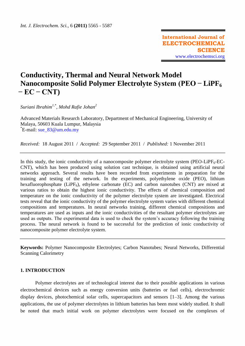
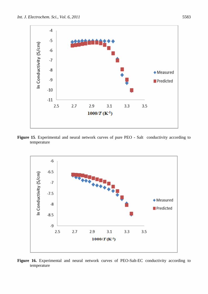
A comparison of the measured and predicted conductivity is presented in Figs. 14 - 19. In these

cases it can be seen that the measured values lie completely within the predicted values. The model is

found to be capable of generalising sufficiently to reproduce the general trends in the data and is

capable of making useful predictions of unseen composition and temperature.

Figure 14. Experimental and neural network curves of pure PEO conductivity according to

temperature


5583

Figure 15. Experimental and neural network curves of pure PEO - Salt conductivity according to

temperature

Figure 16. Experimental and neural network curves of PEO-Salt-EC conductivity according to

temperature


5584

Figure 17. Experimental and neural network curves of PEO-Salt-EC-CNT conductivity according to

temperature

Figure 18. Temperature-dependent conductivity of polymer electrolyte system from experimental data


5585

Figure 19. Temperature-dependent conductivity of polymer electrolyte system obtained from neural

network‟s prediction

5. CONCLUSION

Novel composite solid polymer electrolytes were synthesized successfully via solution-casting

technique. It has been demonstrated in this paper that the addition of various weight percent of salt,

plasticizer and filler into the PEO matrix enhances conductivity. DSC thermographs exhibit a decrease

in Tm, Tg and Xc values, which leads to increased conductivity for composite polymer electrolytes at

298K. A neural networks model has been developed, which can predict the ionic conductivity of

nanocomposite polymer electrolyte systems (PEO - LiPF6 - EC - CNT). The generalized capability of

the neural network is the primary consideration of this paper. The Bayesian neural network is found to

be successful in predicting of experimental results rather that of time-consuming studies.

ACKNOWLEDGEMENT

M. R. Johan is grateful to Academy of Science Malaysia under Brain Gain Program for IFPD

Fellowship 2010 and University of Cambridge, Department of Materials Science and Metallurgist as a

Visiting Scientist (April – July 2010). He also thanks to Professor H. K. D. H. Bhadeshia for the

provision of laboratory facilities at the University of Cambridge and Dr Steve Ooi and Mr Arpan for a

very fruitful discussion on Bayesian Neural Networks Model. Suriani Ibrahim would like to

acknowledge the financial support provided by University of Malaya‟s tutorship scheme and PPP

Grant No PS083/2009B.


5586

References

1. S.A Manuel , P.T. Kumar, N.G. Renganathan, S. Pitchumani, R. Thirunakaran, N. Muniyandi. J

Power Sources 89 (2000) 80.

2. S. Rajendran, P. Sivakumar, R.S. Babu. J Power Sources 164 (2007) 815.

3. S. Rajendran, O. Mahendran, R. Kannan. J Phys Chem Solids 63 (2002) 303.

4. D. Shanmukaraj, R. Murugan. J Power Sources 149 (2005) 90.

5. A.M.M.A. Ali, M.Z.A Yahya, H. Bahron, R.H.Y. Subban, M.K. Harun, I. Atan. Mater. Lett

61(2007) 2026.

6. G.B. Appetecchi, M. Montanino, A. Balducci, S.F. Lux, M. Winterb, S. Passerini. J Power Sources

192 (2009) 599.

7. M.R. Johan, S.H. Oon, S. Ibrahim, S.M.M Yassin, Y.H. Tay. Solid State Ionics.

DOI/org/10.1016/j.ssi.2011.06.001.

8. S. Ibrahim, S.M.M Yassin, R. Ahmad, M.R. Johan, Ionics. 17 (2011) 399.

9. T.S. Min, M.R. Johan. Ionics. 17 (2011) 485.

10. M.R. Johan, L.B. Fen. Ionics. 16 (2010) 335.

11. M.R. Johan, S.A. Jimson, N. Ghazali, N.A.M. Zahari, N.F. Redha. Inter. Nat. Mater. Reas. 102

(2011) 4.

12. D. Saika, Y.M.C. Yang, Y.T. Chen, Y.K. Li, S.I. Lin. Desalin 234 (2008) 24.

13. R.H.Y. Subban, A.K. Arof. J Eur Polym 40 (2004)1841.

14. B. Rupp, M. Schmuck, A. Balducci, M. Winter, W. Kern. J Eur Polym 44 (2008) 2986.

15. S. Ramesh, F.Y. Tai, J.S. Chia. Spectrochim Acta Part A 69 (2008) 670.

16. G.B. Appetecchi, S. Passerini. Electrochim. Act 45 (2000) 2139.

17. M.R. Johan, S. Ibrahim, Communications in Nonlinear Science and Numerical Simulation. 7

(2012) 329.

18. M.R. Johan, S. Ibrahim. Ionics. DOI.1007/s11981-011-0549-z.

19. H.K.D.H. Bhadeshia . ISI J International 39 (1999) 966.

20. H.K.D.H. Bhadeshia, R.C. Dimitriu, S. Forsik, J.H. Park, J.H. Ryu. Mater Sci Tech 25 (2009) 504.

21. D.J.C. MacKay.Neural Comput 4 (1992) 415.

22. D.J.C. MacKay. Neural Comput 4 (1992) 448.

23. D.J.C. MacKay.Network: Comput Neural Syst 6 (1995) 469.

24. M.N. Ng, M.R. Johan, Extended abstracts, IEEE International NanoElectornics Conference 2010

(INEC 2010). Vols 1 & 2. pg 392.

25. S. Rajendran, P. Sivakumar, B.R. Shanker, J Power Sources. 164 (2007) 815.

26. F. Croce, S.D. Brown, S. Greenbaum, S.M. Slane, M. Salomon, Chemistry. Materials. 5 (1993)

1268.

27. G.G. Cameron, M.D. Ingram, K. Sarmouk, Polymer. 26 (1990) 1097.

28. J. Przluski, M. Siekierski, W. Wieczorek, Electrochimica Acta. 40 (1995) 2101.

29. F. Capuano, F. Croce, B. Scrosati, J Electrochemical Society. 138 (1991) 1918.

30. M.C. Borghini, M. Mastrogostino, S. Passerini, B. Scrosati, J Electrochemical Society. 142 (1995)

2118.

31. Z.Y. Wen, T. Itoh, N. Hirata, M. Ikeda, M. Kubo, O. Yamamoto, J Power Sources. 90 (2000) 20.

32. Y.W. Kim, W. Lee, B.K. Choi, Electrochimica Acta 45 (2000) 1473.

33. B. Kumar, L.G. Scanlon, Solid State Ionics 124 (1999) 239.

34. M.P. Anantram, F. Leonard. Reports on Progress in Physics. 69 (2006) 507.

35. B.E. Kilbride, J.N. Coleman, J. Fraysse, P. Fournet, M. Cadek, A. Drury J Applied Physics. 92

(2002) 4024.

36. J. Ulanski, P. Polanowski, A. Traiez, M. Hofmann, E. Dormann, E. Laukhina, Synthetic Metals. 94

(1998) 23.

37. D.K. Pradhan, B.K. Samantaray, R.N.P. Choudhary, A.K. Thakur. Ionics. 11 (2005) 95.


5587

38. A.Ferry, P. Jacobsson, J.D. Van Heumen, J.R. Stevens, Polymer 37 (1996) 737.

39. M.M. Silva, S.C. Barros, M.J. Smith, J.R. MacCallum, Electrochim.Acta 49 (2004) 1887.

40. G. Chiodelli, P. Ferloni, A. Magistris, M. Sanesi, Solid State Ionics 28–30 (1988) 1009.

41. G.B Appeteechi, F. Crose, L. Persi, F. Ronci, B. Scrosati, Electrochim Acta 45 (2001) 1481.

42. S.H Liao, C.Y Yena, C.C Wenga, Y.F Lina, C.C.M. Maa, C.H. Yang, M.C. Tsai, M.Y Yena, M.C

Hsiao, S.J. Leed, X.F. Xiee, Y.H. Hsiao. J Power Sources 185 (2008) 1225.

© 2011 by ESG (www.electrochemsci.org)

http://www.electrochemsci.org/

conductivity, thermal and neural network model ... · pdf fileconductivity, thermal and neural...

Documents