Conditional Value at Risk Asset Allocation

A Copula Based Approach

Hamed Naeini

A Thesis in

John Molson School of Business

Presented in Partial Fulfillment of the Requirements

for the Degree of Master in Science (Administration) at

Concordia University

Montreal, Quebec, Canada

December 2013

© Hamed Naeini, 2013

CONCORDIA UNIVERSITY

School of Graduate Studies

This is to certify that the thesis prepared

By: Hamed Naeini

Entitled: Conditional Value at Risk Asset Allocation, a Copula Based Approach

and submitted in partial fulfillment of the requirements for the degree of

Master in Administration (Finance)

complies with the regulations of the University and meets the accepted standards with

respect to originality and quality.

Signed by the final Examining Committee:

Professor Mahesh Sharma Chair

Professor Ravi Mateti Examiner

Professor Rahul Ravi Examiner

Professor Thomas J. Walker Supervisor

Approved by _______________________________________________

Chair of Department or Graduate Program Director

_______________2013 ______________________

Dean of Faculty

iii

Abstract

Conditional Value at Risk Asset Allocation

A Copula Based Approach

Hamed Naeini

The title of this thesis is Conditional Value at Risk Asset Allocation, A Copula Based

Method, and it is written by Hamed Naeini. The thesis supervisor is Professor Thomas J.

Walker. Using a non-parametric bootstrapping method, we allocate funds to eleven

preselected asset classes based on a series of conditional value at risk and variance

criteria. Next, we employ copulas to model the data and build our comparison portfolios.

We compare the results of the two methods during both bull and bear markets conditions.

We find that model-based asset allocation significantly improves the performance of

portfolios during financial crises. Under normal market conditions, the two methods

result in comparable performance. We conclude that our optimization procedure provides

asset allocation strategies that result in portfolios that perform at least as well as

portfolios constructed based on the commonly used bootstrapping method and

significantly better during periods of financial turmoil.

iv

Acknowledgement

I would like to express my deepest appreciation to my supervisor, Professor

Thomas J. Walker, for his encouraging words, thoughtful criticism, and time and

attention during busy semesters, and for all I have learned from him and for his

continuous help and support in all stages of this thesis. I would also like to thank

him for being an open person to ideas, and for encouraging and helping me to

shape my interest and ideas.

I would like to thank my committee members, Professor Ravi Mateti, and

Professor Rahul Ravi whose advices and insight was invaluable to me. In addition,

special thanks go to Professor Kuntara Pukthuanthong; it would not have been

possible to write this thesis without her help.

Finally, I would like to thank my family, specially my wife, for always

believing in me, for her continuous love and her supports in my decisions.

Moreover, I would like to thank my father and my mother, for their support during

my life. Without whom I could not have made it here.

v

Table of Contents

1-Introduction & Literature Review ....................................................................... 1

1.2-Value at Risk ................................................................................................ 2

1.3-Conditional Value at Risk............................................................................. 3

1.3.1-Optimization of Conditional Value at Risk ........................................... 5

1.4-Asset Allocation ........................................................................................... 7

1.5-A Brief on Risk Management ..................................................................... 10

2-Data .................................................................................................................... 13

3-Bootstrapping CVaR and MVO Portfolios ........................................................ 16

4-Modeling the Data ............................................................................................. 19

4.1-Modeling the Univariate Statistical Distribution of Asset Returns ............ 20

4.2-Modeling the Dependence Structure of Asset Returns ............................... 26

4.3-Simulating from Estimated Models ............................................................ 31

5-Results ............................................................................................................... 32

5.1-2008 Optimization Results ......................................................................... 33

5.1.1-Historical Means .................................................................................. 33

5.1.2-Black-Litterman Implied Means .......................................................... 34

5.2-2013 Optimization Results ......................................................................... 36

5.2.1-Historical Means .................................................................................. 36

5.2.2-Black-Litterman Implied Means .......................................................... 37

vi

6-Further Analysis ................................................................................................ 38

7-Conclusions ....................................................................................................... 39

8-Venues for Future Research .............................................................................. 41

References ............................................................................................................. 42

Appendix ............................................................................................................... 66

vii

LIST OF TABLES

Table 1- Asset classes and their relevant indices .................................................. 45

Table 2- Descriptive statistics for the data ............................................................ 46

Table 3- Parameter estimation for AR(2)-GARCH(1,1) model ........................... 47

Table 4- Parameter estimation for Hansen’s skewed t distribution ...................... 49

Table 5- Parameter estimation for the copulas ..................................................... 50

Table 6- Performance summary of CVaR optimizations with the historical means

2008/2009 ......................................................................................................................... 51

Table 7- Performance summary of CVaR optimizations with the implied Black-

Litterman means 2008/2009 ............................................................................................. 52

Table 8- Performance summary of CVaR optimizations with the historical means

2013................................................................................................................................... 53

Table 9- Performance summary of CVaR optimizations with the implied Black-

Litterman means 2013....................................................................................................... 54

viii

List of Figures

Figure 1- Normal quantile-quantile plots .............................................................. 55

Figure 2- Quantile-quantile plots based on Hansen skewed t ............................... 57

Figure 3- : Performance summary of CVaR optimizations with the historical

means 2008/2009 .............................................................................................................. 59

Figure 4- Performance summary of CVaR optimizations with the implied Black-

Litterman means 2008/2009 ............................................................................................. 60

Figure 5- : Performance summary of CVaR optimizations with the historical

means 2013 ....................................................................................................................... 61

Figure 6- : Performance summary of CVaR optimizations with the implied Black-

Litterman means 2013....................................................................................................... 62

Figure 7- evolution of the dynamic correlation between U.S. bonds and U.S.

equities .............................................................................................................................. 63

Figure 8- evolution of the dynamic correlation between U.S REITs and small cap

equities .............................................................................................................................. 64

Figure 9- evolution of the dynamic correlation between commodities and equities

........................................................................................................................................... 65

1

1-Introduction & Literature Review

The notion of risk has a long history in the financial literature, and here are

several measures that are frequently used to quantify risk. However, there is no consensus

among academics and practitioners about which measure is the best. The trade-off

between risk and return is a fundamental concept in asset pricing and portfolio

management. Thus, there have been many attempts to define a risk measure since the

early days of financial research. Roy (1952) and Markowitz (1959) presented two of the

first risk measures in the 1950s, which are still in use. More complex risk measures were

not introduced until the late 1980s.

Generally speaking, risk measures can be divided into two categories. The first

category includes dispersion-based risk measures. The most well-known members of

this category are the variance and standard deviation of a portfolio’s time series returns.

These risk measures quantify the uncertainty of portfolio returns around their expected

value. One drawback of the measures is that they treat both positive and negative returns

the same way. This draw back leads to the introduction of a new class of dispersion risk

measures: downside dispersion risk. Semi-variance and Roy’s safety-first criterion are

examples of this class.

The second category includes downside risk measures. These risk measures are

based on the fact that the return on an asset is a random variable. The risk of a portfolio is

quantified using the percentiles of the portfolio’s return distribution. This concept is

consistent with the preferences of risk-averse investors. These types of risk measures

have captured a lot of attention from both academics and practitioners since the late

1980s. The most famous risk measure in this category is Value at Risk (VaR). A related

2

risk measure, Conditional Value at Risk (CVaR a.k.a. Expected Shortfall) was

introduced in the 1990s (for instance, Balzer, 1994). The latter risk measure is the subject

of interest in this paper. However, before discussing CVaR, one should have a good

understanding of VaR. Consequently, in the next section, we will start by discussing

VaR.

1.2-Value at Risk

Value-at-risk (VaR) measures the predicted maximum portfolio loss at a certain

probability level ( ) over a certain time horizon. Common probability levels are 1 and 5

percent, and common time horizons are 1 and 10 days. VaR can be stated in both dollar

and percentage terms. In this document, we use percentage terms, as they are more

prevalent in the academic literature. Figure below shows the VaR for a generic return

distribution of a portfolio. The mathematical definition of Value at Risk is:

( )

One of the first practical uses of Value at Risk was implemented by J.P. Morgan.

When Dennis Weatherstone, the then-chairman of J.P. Morgan, tried to establish an

integrated risk management system, he ordered his employees to provide a one-page

3

report, which explains the firm wide-risk over the next day with respect to the bank’s

entire trading portfolio. The “4:15” report (because the report was delivered at the end of

each trading day) used VaR to assess the potential risk the firm may encounter the next

day.

The simplest method of calculating VaR is to use a normal distribution to model

portfolio returns. However, it is well documented in the literature that normality is not a

realistic assumption. Therefore, alternative methods have been presented for calculating

VaR. Historical simulations and Monte Carlo simulations are examples of other VaR

calculation methods.

Although the use of VaR is very wide-spread in the financial industry, VaR

suffers from some important drawbacks. First, VaR is silent about the amount of losses if

a low probability event in the left tail of the distribution occurs. Second, Artzner et al.

(1999) show that using VaR as a risk measure to allocate funds to assets in portfolios can

lead to poor decision and portfolios that are not well diversified. Finally, portfolio

optimization based on VaR is a very difficult process and often requires the use of

complicated techniques. Nassim Taleb (2007) discusses many arguments against using

VaR in his famous book, Black Swan.

1.3-Conditional Value at Risk

As previously mentioned, VaR has some strengths and drawbacks. The ability to

quantify the risks a firm faces in a single risk measure is an interesting property.

However, this one single measure may neglect very important information about big

losses. These arguments lead to the introduction of a new risk measure, Conditional

4

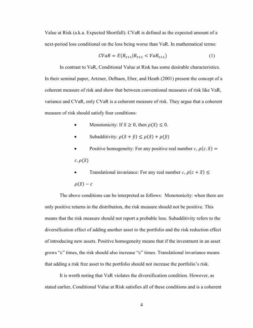
Value at Risk (a.k.a. Expected Shortfall). CVaR is defined as the expected amount of a

next-period loss conditional on the loss being worse than VaR. In mathematical terms:

( | ) (1)

In contrast to VaR, Conditional Value at Risk has some desirable characteristics.

In their seminal paper, Artzner, Delbaen, Eber, and Heath (2001) present the concept of a

coherent measure of risk and show that between conventional measures of risk like VaR,

variance and CVaR, only CVaR is a coherent measure of risk. They argue that a coherent

measure of risk should satisfy four conditions:

Monotonicity: If ͂ , then ( ͂)

Subadditivity: ( ͂ ͂) ( ͂) ( ͂)

Positive homogeneity: For any positive real number c, ( ͂)

( ͂)

Translational invariance: For any real number c, ( ͂)

( ͂)

The above conditions can be interpreted as follows: Monotonicity: when there are

only positive returns in the distribution, the risk measure should not be positive. This

means that the risk measure should not report a probable loss. Subadditivity refers to the

diversification effect of adding another asset to the portfolio and the risk reduction effect

of introducing new assets. Positive homogeneity means that if the investment in an asset

grows “c” times, the risk should also increase “c” times. Translational invariance means

that adding a risk free asset to the portfolio should not increase the portfolio’s risk.

It is worth noting that VaR violates the diversification condition. However, as

stated earlier, Conditional Value at Risk satisfies all of these conditions and is a coherent

5

measure of risk. Notice that even standard deviation cannot satisfy all of the conditions. It

is not zero when all the returns in the distribution are positive. Consequently, it seems

that CVaR is a more reliable risk measure than VaR or variance.

Another important benefit of CVaR relative to standard deviation and variance is

that asset returns are not normally distributed; therefore, standard deviation cannot

describe the distribution characteristics completely. In contrast to standard deviation,

CVaR contains almost all of the information about the asset return distribution.

Specifically, CVaR considers the information on both the kurtosis and skewness of asset

returns. Thus, CVaR is an ideally suited risk measure for handling heavy tailed

distributions.

Moreover, the optimization of a portfolio based on CVaR is relatively easy.

Rockafellar and Uryasev (2000) propose a simple scenario-based algorithm for CVaR

optimization. The beauty of their algorithm is that there is no need to assume a specific

distribution for returns in the optimization process. Moreover, the optimization is a

typical linear programming problem and is even simpler than the quadratic optimization

problem of variance optimization. In the next section, this algorithm will be discussed in

more detail.

1.3.1-Optimization of Conditional Value at Risk

Suppose that we have a portfolio of n assets. The CVaR of this portfolio depends

on two things: first, the weights of each individual asset and second, their return

distribution. The return of the portfolio is equal to , where, r is a vector of

expected asset returns and w is a vector of asset weights. The 100(1 − ε)% CVaR of the

portfolio can be written mathematically as:

6

( )

∫ ( ) ( )

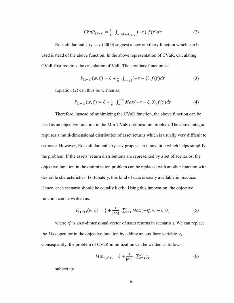
( ) (2)

Rockafellar and Uryasev (2000) suggest a new auxiliary function which can be

used instead of the above function. In the above representation of CVaR, calculating

CVaR first requires the calculation of VaR. The auxiliary function is:

( )( )

∫ ( ) ( )

(3)

Equation (2) can thus be written as:

( )( )

∫ ( ) ( )

(4)

Therefore, instead of minimizing the CVaR function, the above function can be

used as an objective function in the Min-CVaR optimization problem. The above integral

requires a multi-dimensional distribution of asset returns which is usually very difficult to

estimate. However, Rockafellar and Uryasev propose an innovation which helps simplify

the problem. If the assets’ return distributions are represented by a set of scenarios, the

objective function in the optimization problem can be replaced with another function with

desirable characteristics. Fortunately, this kind of data is easily available in practice.

Hence, each scenario should be equally likely. Using this innovation, the objective

function can be written as:

( )( )

∑ (

) (5)

where is an n-dimensional vector of asset returns in scenario s. We can replace

the Max operator in the objective function by adding an auxiliary variable .

Consequently, the problem of CVaR minimization can be written as follows:

∑

(6)

subject to:

7

It is worth noting that when the asset distribution is normal, both MVO and CVaR

optimization produce the same answers. Other limitations (p.g. a minimum level of

expected returns) can be added to the above problem. The beauty of this formulation is

that the above problem becomes a linear optimization problem, and can be easily handled

when the dimension of the problem is small. Using CVAR in asset allocation until

recently has not grasped much attention from practitioners, although it is a common and

increasingly popular risk measure in the risk management literature.

1.4-Asset Allocation

The problem of how to allocate funds to different asset classes is as old as the

capital markets themselves. Many methods for asset allocation have been presented

during the twentieth century, from a naïve diversification approach (equal weights) to

experienced-based models and complicated Bayesian asset allocation models. The

fundamental assumption of most of these methods is that asset returns are normally

distributed. However, this assumption is not realistic. The most famous asset allocation

model is the mean-variance asset allocation model developed by Markowitz (1959).

Under this approach, an investor tries to allocate funds at each level of expected return,

with a minimum variance condition. The resulting curve depicting the respective

portfolios is called the efficient frontier. One of the main drawbacks of MVO asset

allocation is that the resulting efficient frontier is not stable. Some work has been done to

overcome this problem. For instance, Michaud (1989) presents a sampling method to

8

construct a stable efficient frontier. This bootstrapping process builds a distribution for

the efficient frontier. However, there is no sound theoretical basis for this method and no

statistical reasoning exists to verify that the portfolio constructed based on a resampling

method should be superior to traditional MVO portfolios.

The problem of unstable efficient frontiers remained unsolved until the seminal

work of Black and Litterman (1992). In their paper, they present a Bayesian approach to

estimate the expected returns of asset classes. Instead of using average historical returns

as a proxy for expected returns, they use observable asset weights to estimate expected

asset returns. Although they rely on a historical covariance matrix of asset returns, their

efficient frontier is more stable when compared to traditional mean-variance

optimization. The reason is that the efficient frontier is highly sensitive to expected

returns, while its sensitivity to covariance and variance is much lower. Along with

solving the problem of unstable efficient frontiers, their model allows asset managers to

incorporate their beliefs into the asset allocation problem using a Bayesian process.

Most asset allocation models are developed based on the normality assumption.

Consequently, the main risk measure in these models is variance or standard deviation.

When the normality assumption is relaxed, there is a need for other risk measures to

incorporate higher moments of the return distribution. For instance, Campbell et al.

(2001) develop an asset allocation model based on Value at Risk in which they minimize

the VaR for each level of return. Nevertheless, as mentioned previously, VaR may lead to

undiversified portfolios. The use of a coherent measure of risk such as CVaR in making

asset allocation decisions is still rare in the financial industry even though it has been ten

years since its introduction.

9

The first asset allocation problem that uses CVaR as a risk measure is presented

by Uryasev et al. (2001). The authors utilize a CVaR optimization process to develop an

asset allocation model for a pension fund. The pension fund asset allocation problem

differs in two respects from traditional asset allocation problems. First, most pension

funds face a multi-period time horizon in their investment decisions. Second and more

importantly, these funds use an asset/liability approach, instead of an asset-only

approach.

After Uryasev et al’s (2001) original study, there was no noteworthy paper about

CVaR in the finance literature until recently. In fact, most early research on CVaR

optimization was done in the operations research literature. Hu and Kercheval (2009)

develop a model based on a multivariate t distribution and a multivariate skewed t

distribution for asset returns, and use the CVaR optimization process to construct an

efficient frontier. Nevertheless, their work is limited to estimating a model for five stocks

in the Dow Jones index, and they do not investigate different asset classes. Moreover, the

use of a multivariate distribution has its own drawbacks. For instance, the skewness

parameter in a multivariate skewed student t distribution should capture both the

skewness of each asset and the skewness of the dependence structure among assets.

The first paper that uses Uryasev’s method to handle a real asset allocation

problem is a recent paper by Idzorek and Xiong (2011). In that paper, the authors first

present five hypothetical assets with different skewness and kurtosis values and show that

when skewness and kurtosis exist in asset return distributions, a CVaR asset allocation is

superior to mean-variance optimization. Second, they use a relatively simple

bootstrapping methodology and construct portfolios for four levels of expected returns.

10

They find that for assets with heavier tails such as small cap growth stocks, the weights

that result from a CVaR optimization are significantly different from a mean variance

optimization. Furthermore, they document better performance for a portfolio constructed

based on CVaR constraints when compared with variance constraints during the 2008

financial crisis.

1.5-A Brief on Risk Management

The use of CVaR and CVaR optimization is more conventional in the risk

management literature. CVaR is a risk measure that scholars usually recommend to be

used in conjunction with VaR to present a realistic picture of the risk a company faces. It

is also a risk measure that is frequently used in integrated risk management. There have

been several papers in recent years, which use CVaR optimization in their methodology.

For instance, Jin (2009) uses a CVaR optimization process to evaluate the risk of large

portfolios. He uses copulas to model dependencies among portfolio risk factors.

Christoffersen and Langlois (2011) use a copula-based approach to model dependencies

between equity market factors (namely, Fama-French factors). Finally, Christoffersen et

al. (2012) survey the potential for international diversification using copula-based

methods.

This paper exteds these recent works. Moreover, we employ some of the concepts

and techniques used in risk management to model and simulate asset returns. The

information and related literature for each of the models we will use in our subsequent

analysis are discussed in each related section.

The method we use in this paper has characteristics that should make it preferable

to the bootstrapping method used by Idzorek and Xiong (2011). First, one of the main

11

assumptions in bootstrapping is that each draw is independent from the other.

Unfortunately, this is not the case for asset returns, especially when using daily data,

because of the existence of volatility clustering in the data.

Moreover, as CVaR optimization is a scenario-based optimization method,

meaning that we use data points to estimate the real distribution of data. The more data

we have on hand, the better are the optimization results we produce. This issue should be

given some attention due to the fact that tail data are very important in the CVaR

optimization process and they are rare by nature (thus lending them their nickname Black

Swans). Bootstrapping may not collect a sufficient amount of data in tails and the

optimization may suffer because of the lack of tail information. In contrast, in simulations

any number of tail information can be generated.

In addition to these independence and tail information scarcity problems,

bootstrapping cannot provide much information about our portfolios. Specifically,

bootstrapping is not able to handle portfolio optimization involving tactical asset

allocation or active portfolio management. For instance, a question such as what would

happen to the risk of a portfolio if the weight of one asset class were reduced cannot be

answered in a bootstrapping framework. Moreover, bootstrapping only provides average

results. For example, the VaR in a bootstrapping framework will be the average of many

years of data and may be very different from the real VaR under current market

conditions. The parametric model we use in this study is updated daily, and previous up-

to-date estimates for risk measures are available for the subsequent day after the closing

bell of each trading day. In summary, we believe that it is worth developing a parametric

12

model to approach this problem and we hope this model generates better results than the

bootstrapping method.

Our paper is organized as follows. In the next section, we describe the data we use

in this study. Section 3 is dedicated to the construction of portfolios based on the

methodology proposed by Idzorek and Xiong (2011). In Section 4, we model asset

returns based on methodologies that are frequently used in the risk management

literature. First, we use a conditional mean and volatility model to model the time varying

variance of each asset return time-series. Second, we model the marginal shocks in asset

returns using proper statistical distributions. Third, we model the dependence structure of

these marginal distributions using copulas. Fourth, we simulate asset return time-series

based on the model and use CVaR optimization to build portfolios. In section 5, we

compare the results we obtained under the MVO and CVaR optimization methods with

the results of Idzorek and Xiong (2011). Section 6 covers a closer look into the

correlation among assets. Finally, section 7 concludes. The last section presents some

venues for future research.

13

2-Data

The objective of this research is to present a parametric model that extends the

non-parametric bootstrapping method used in Idzorek and Xiong (2011). Thus, we collect

data that are as close as possible to Xiong and Idzorek’s (2011) original paper.

Nevertheless, the data we could obtain during our sample formation differs in some

respect from Idzorek and Xiong (2011). Specifically, they use 14 asset classes, which are

available for sophisticated institutional investors. The asset classes and indices used to

represent them in our research are presented in Table 1. Note that all of the indices are

investable indices, and there are both ETFs and mutual funds that can be used to invest in

these indices. All data, including price and market caps information for each index, are

collected from Thomson Reuters’ DataStream. We tried to collect data in the same time

interval as the original paper. Nevertheless, we could not go back to 1990, because the

data was not available. Moreover, we had to modify some of the indices used by Idzorek

and Xiong (2011). An important difference between our equity returns and the Xiong and

Idzorek’s equity return is that we use price returns instead of total returns because total

return data is only available after 2000. Subject to these limitations, we collect data for

the longest time span available. Our data starts on June 1, 1993. Therefore, when

modeling for the year 2008, we have 15 years of prior data. In our analysis, we employ

daily log returns which are calculated as follows:

(

⁄ ) (7)

*** Insert Table 1 about here ***

14

We briefly explain each of the asset classes we use in this study and their related indices

below.

Russell 1000 Value Index

This index measures the performance of large companies in the US market with

low price to book ratios. The low price to book ratio implies that the market has a low

expected growth rate for these companies. The average market cap of a company in this

index is 102.875 billion dollars in 2013. The reconstitution frequency is annually. This

index primarily contains blue chip companies such as Exxon Mobil and GE.

Russell 1000 Growth Index

This index is a large cap index; however, companies listed in the index have

above-average expectations for growth. The average market cap of a company in this

index is 88.512 billion dollars in 2013. Reconstitution is done annually and the most

famous members of this index are Apple Inc. and Microsoft Corp.

Russell 2000 Value Index

This index is designed to mimic the performance of small cap companies with

low expected growth. The average market cap of a company in this index is 1.4 billion

dollars. The Russell 2000 Value Index contains many small financial companies.

Russell 2000 Growth Index

The index is similar to the Russell 2000 Value Index, yet the price to book ratio

for firms in this index is generally higher. The average size of a company in this index is

1.858 billion dollars. Firms in the health care industry constitute a large portion of this

index.

MSCI World ex USA Index

15

This index is designed to capture the performance of developed equity markets

other than the U.S. This index contains 7,891 firms from 23 developed countries. The

combined market cap of firms in this index is around 16 trillion dollars, and the average

size of a firm in this index is 2 billion dollars.

MSCI Emerging Markets Index

This index measures the performance of developing countries. The index covers

firms from 21 countries, which are in Latin America and South East Asia. The number of

securities in this index is around 800.

S&P GSCI Commodity Index

This index is a well-known benchmark for investing in the commodity market.

The index has very diverse components, from crude oil and precious metals to livestock.

The index has a strong exposure to energy-linked commodities relative to other

commodity indices. The index is constructed using futures contracts. Consequently, the

true market cap of the index is zero. However, there is ongoing research about the

allocation to commodity indices in the asset allocation literature.

FTSE EPRA/NAREIT U.S. Index

This index measures the performance of real estate investment trusts which are

listed in the U.S. Although the index does not cover the entire real estate market in the

United States, it is a good barometer for the performance of this asset class.

Barclays Capital U.S. Aggregate Bond Index

The Barclays Capital Aggregate Bond Index, formerly known as the Lehman

Aggregate Bond Index, aims to capture the performance of the investment grade sector of

the U.S. bond market. The index includes Treasury issues. The average maturity of bonds

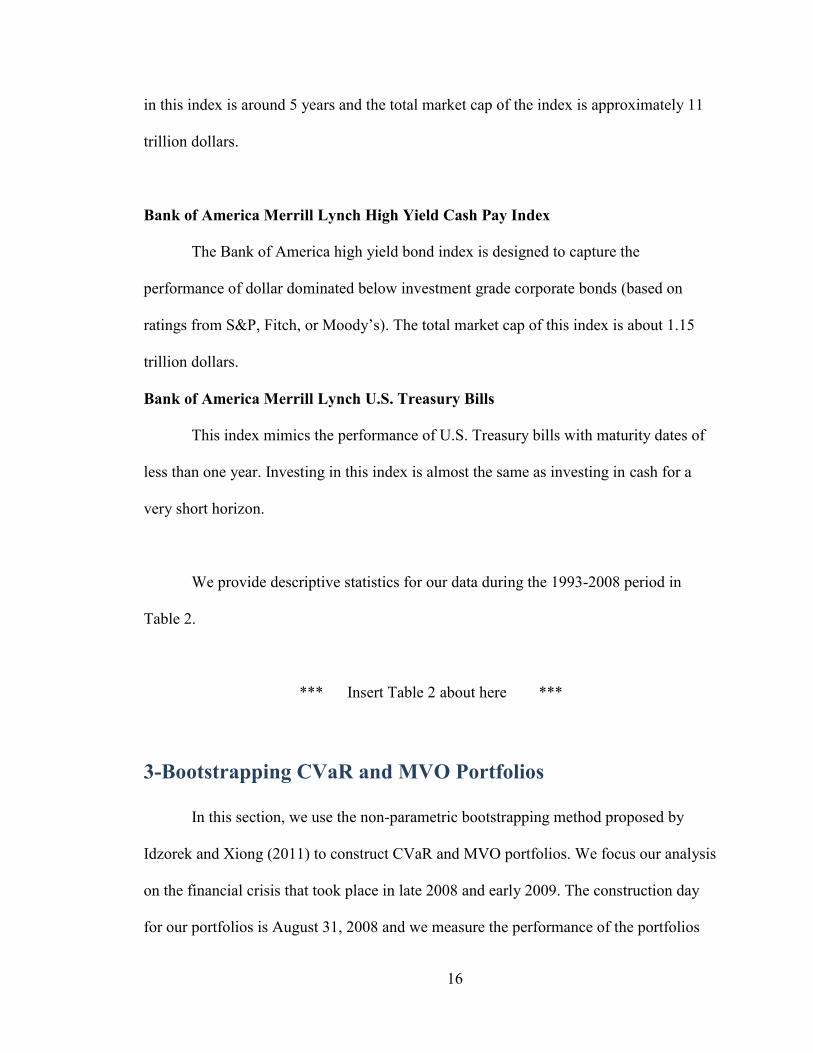
16

in this index is around 5 years and the total market cap of the index is approximately 11

trillion dollars.

Bank of America Merrill Lynch High Yield Cash Pay Index

The Bank of America high yield bond index is designed to capture the

performance of dollar dominated below investment grade corporate bonds (based on

ratings from S&P, Fitch, or Moody’s). The total market cap of this index is about 1.15

trillion dollars.

Bank of America Merrill Lynch U.S. Treasury Bills

This index mimics the performance of U.S. Treasury bills with maturity dates of

less than one year. Investing in this index is almost the same as investing in cash for a

very short horizon.

We provide descriptive statistics for our data during the 1993-2008 period in

Table 2.

*** Insert Table 2 about here ***

3-Bootstrapping CVaR and MVO Portfolios

In this section, we use the non-parametric bootstrapping method proposed by

Idzorek and Xiong (2011) to construct CVaR and MVO portfolios. We focus our analysis

on the financial crisis that took place in late 2008 and early 2009. The construction day

for our portfolios is August 31, 2008 and we measure the performance of the portfolios

17

for the subsequent six-month period. Consequently, our realized return is calculated on

the last day of February 2009. During this six-month period the financial markets

experienced the worst crisis in recent memory, and most asset classes were subject to a

huge decline in their value. For instance, U.S. REITs lost more than 60 percent of their

value during this period.

The most crucial parameter in every portfolio optimization is the estimation of

expected asset returns. Chopra and Ziemba (1993) document that at a moderate risk

tolerance level, MVO is much more (about 11 times) sensitive to expected return

estimations than to risk estimations (variance). Therefore, portfolios are constructed using

two different approaches: in the first approach, historical means of asset classes are used

as estimates of ex-ante means of asset returns. In the second approach, Black-Litterman

equilibrium expected returns are used as estimates of ex-ante asset returns. Using Black-

Litterman expected returns, the mean of data should be readjusted by the difference

between the Black-Litterman expected return and the historical mean of data. Black and

Litterman use reverse optimization to calculate the expected returns from observable

parameters in the market. Their formula is based on the capitalization weights of asset

classes. Hence, given the aforementioned difficulties in estimating the market cap for a

commodity index, which is beyond the scope of this study, the commodity index is

removed from portfolios constructed based on the Black-Litterman approach.

For historical expected return optimizations, six sets of portfolios are constructed

based on required returns of 4% to 9%. Moreover, six sets of portfolios are built based on

Black-Litterman expected returns. These annual required returns are converted to daily

returns based on a 250 trading day year. The reason for adding two portfolios with four

18

and five required returns to the Black-Litterman (BL) analysis is that based on BL

estimated returns, portfolios with required returns of eight and nine percent are very

aggressive in terms of risk.

Bootstrapping is concluded as follows. For each portfolio with a specific required

return, 500 samples are collected. Each sample contains 244 draws (we used the same

number of draws as in Idzorek and Xiong (2011)) from raw asset returns. Each sample is

used to construct a CVaR and mean variance (MV) optimized portfolio. The optimized

weights for each sample are documented. These weights are averaged and presented as

the optimal weights for both the CVaR and MV optimized portfolios for each level of

required return. The detailed results are not reported here, but are available upon request.

*** Refer to Table 1A in the Appendix here ***

*** Refer to Table 6A in the Appendix here ***

As can be seen from our results, in most cases CVaR optimization beats the

results of MVO. The performance improvement is particularly significant when

employing the Black-Litterman approach (cf., Idzorek and Xiong, 2011). As expected,

CVaR optimization allocates fewer funds to assets with more negative skewness and

fatter left tails. For example, the allocated weight to large-cap value stocks is lower in

CVaR optimization when compared to MVO in both Black-Litterman and historical

mean portfolios. When examining the performance differences of the two methods in

estimating ex-ante means in the historical mean expected return (refer to table 1A in the

Appendix), CVaR optimization results is a 133 basis point higher return than MVO for a

19

portfolio with a required return of seven percent. This difference is 448 basis points or

almost 4.5 percent for the associated Black-Litterman portfolio.

Although the weights in portfolios with historical expected means are very

different from the weights of a passive market portfolio, the realized losses for this

portfolio type are much lower than for portfolios that are constructed based on the BL

approach. For instance, in BL portfolios with a six percent required return, the loss is

almost four times higher than the loss for the non-BL counterpart in the historical

expected return portfolio.

4-Modeling the Data

In this section, we start to model the time series of asset returns. Afterwards, we

will use this model to construct simulated returns based on this model that we will use in

our optimization problem. A lot of research has been done in this area. Modeling asset

returns is one of the main topics in the risk management literature, thus we utilize risk

management methodologies to model our data.

The first and most simplistic assumption about asset returns is that they are

distributed following a multivariate Gaussian distribution. This means not only that each

asset return is normally distributed, but also that the dependence structure of asset returns

is normal and that linear correlations are enough to describe the behaviour of asset

returns. However, it is a well-known fact that assuming a normal distribution has serious

weaknesses when modeling both a univariate asset return time-series and the dependence

structure among asset returns. Granger (2002) studies the performance of multivariate

normal distributions and concludes that a normal distribution can not explain the stylized

facts about the returns observed in economic time series. Similarly, other multivariate

20

distributions have been explored in the literature. For instance, Hu and Kercheval (2009)

model asset returns using multivariate student t and skewed student t distributions.

However, using multivariate distributions is a very limiting method. For example,

assuming that all time series follow a particular univariate distribution with the same

parameters is not very acceptable. Moreover, in Hu and Kercheval’s modeling method,

the skew parameter in the skewed t distribution should both capture the skewness of all

univariate return time series and the skewness of the dependence structure among them.

Therefore, if different asset classes with different characteristics (namely bonds and

stocks) need to be modeled with this method, the model parameters may not be accurate

estimates. In a nutshell, relying on multivariate distributions to model asset return time

series may not be the best choice, particularly when there are completely different asset

classes among the data to be modeled.

Fortunately, there is a statistical method that allows us to separate the modeling of

univariate distributions from modeling their dependence structure. The so-called copula

function models the dependence structure (and only the dependence structure) among

asset returns. Consequently, each individual asset can have its own specific statistical

distribution. This not only means that each univariate asset distribution can have different

parameters, but also that they can have completely different statistical distributions. In the

following sections, we proceed as follows. First, we model the univariate distribution of

asset returns, and afterwards the dependence among them using a copula function.

4.1-Modeling the Univariate Statistical Distribution of Asset Returns

In this section, we present a framework to model each univariate distribution of

asset returns. In Figure 1A in the Appendix, we display the time series graphs for each

21

asset return. As can be observed in these graphs, the time series are mean reverting.

Therefore, we use a conditional mean model to capture any permanent time series

components.

In addition to modeling the conditional mean of each time series, we have to

account for the well-documented fact that financial time series have volatility clustering.

In other words, the variance of daily returns displays positive autocorrelation. This means

that periods of high volatility tend to be followed by further high volatility periods. This

was one of our critiques of the bootstrapping method, because volatility clustering in

returns is contrary to the independence assumption of bootstrapping. Therefore, before

proceeding to estimate the statistical distributions for our time series, we should first

address this issue and offer a conditional volatility model to capture the volatility

clustering. We use an autoregressive model with GARCH variance as follows:

( ) ( ) (8)

GARCH models were first introduced in the finance literature by Engle (1982).

Since then, a lot of research has been done to model the variance of economic time series.

Andersen et al. (2007) provides a very thorough review of volatility models that are used

in risk management.

One of the main issues that should be considered in modeling volatility is that

negative returns increase volatility more than equally sized positive return. This

phenomenon is referred to as the leverage effect. There are some theoretical justifications

for this effect. For instance, it is often argued that when a firm experiences a negative

return, the value of its equity decreases. Consequently, the debt to equity ratio of the firm

22

increases and therefore the firm becomes more risky. To summerize, a good volatility

model should be able to capture the leverage effect.

As discussed above, we employ a GARCH (1,1) volatility model, which means

that we are using just one lag of the return and variance to model the conditional

volatility. Hansen and Lunde (2005) survey different volatility models with different

orders of lags and conclude that in almost all cases, GARCH models with just one lag are

good enough to model the volatility of the time series.

The GARCH model we employ in this research is the GJR-GARCH (1,1) model,

which was first presented by Glosten, Jagannathan and Runkle (1993). The complete

form of our conditional mean and variance model is illustrated below:

(9)

To ensure that the variance model is stationary, the following condition must be

satisfied:

(10)

There are two ways to estimate the above model. The first is to use OLS to

estimate and . However, some studies show that OLS may not be the best estimator

for this type of model because of the heteroskedasity in residuals. The second and more

justified way is to estimate and using Maximum Likelihood Estimation (MLE).

Likewise, the GJR-GARCH model is estimated by MLE. A good review of AR-GARCH

models can be found in Li, Ling and McAleer (2001). The parameter estimates are

presented in Table 3.

23

*** Insert Table 3 about here ***

To summarize, first we estimate a conditional mean model and after that, we fit a

volatility model on the residuals of the conditional model. The next step is to fit a

statistical distribution on from the above estimated model.

In financial markets, we observe large negative returns while positive large

returns are less frequent and smaller in magnitude than negative returns. Therefore, one

well-known fact about asset returns is that they have negative skewness and fat tails,

which means that the probability of very big losses is larger than what a normal

distribution would predict. Consequently, other statistical distributions are often proposed

to model financial return data. Two of these distributions are the generalized error

distribution and the student t distribution. However, both of them have some serious

weaknesses. The student t distribution and generalized error distribution are symmetric

distributions and cannot model the negative skewness observed in asset returns.

Fortunately, Hansen (1994) presents a skewed version of the student t distribution, which

since its introduction has become the most prominent model used in modeling univariate

asset returns.

We utilize Hansen’s skewed t distribution to model the calculated shocks from the

conditional mean and variance models that are fitted to asset returns. Hansen’s student t

distribution is actually a combination of two different symmetric student t distributions.

The distribution has two parameters; the first one is the degree of freedom ( ), which

should be larger than two and the second one is the skewness parameter ( ), which is

24

bounded between one and minus one. To write the probability density function of the

skewed t distribution, we first define three parameters:

√

(( ) )

( )√ ( ) (11)

where () is the Gamma function. Now we can define the probability density

function of the skewed t distribution as follows:

( ) (12)

[ ( )

(( ) ( ))⁄ ]

( )

[ ( )

(( ) ( ))⁄ ]

( )

The parameters of the skewed t distribution can be estimated using two methods.

The first approach relies on the method of moments. This means that we calculate the

skewness and kurtosis of the observed data and use them as the parametric moments of

the distribution. This method requires solving a non-linear set of equations and may result

in inaccurate estimates. The second method uses Maximum Likelihood Estimation

(MLE). MLE needs an optimization solver, but it is generally more accurate.

To check the goodness of fit of our estimated distributions, we employ a tool that

is popular in the risk management literature, namely quintile-quintile (QQ) plots. The

idea behind QQ plots is that the quintile of one’s empirical results are plotted against the

theoretical quintiles of the desired distribution. If the proposed distribution is a good fit

for the empirical results, then the plot should fall on a line with a slope of one. Figure 1

shows the normal quintile-quintile plots for our sample.

25

*** Insert Figure 1 about here ***

We observe serious departures of non-normality in these plots. Even after fitting

the conditional mean and variance model on the data, the normal QQ plots still exhibit

non-normality (these plots are not displayed for brevity), and the conditional mean and

variance model cannot capture all of the skewness and kurtosis present in the empirical

time series.

In the last step, a skewed student t distribution is fitted to each time series. The

QQ plots for the empirical and theoretical quintiles of the skewed student t distribution

are shown in figure 2.

*** Insert Figure 2 about here ***

The plots exhibit a significant improvement in the goodness of fit. All of the QQ

plots now show a line with a 45-degree angle, suggesting that our parameter estimates are

good estimates of the true parameters of the skewed t distribution.

After completing our first phase of modeling asset returns, we can simulate any

amount of data points from each univariate distribution. Specifically, we generate N

random numbers from a uniform distribution in the [0,1] interval, and use the inverse of

the skewed t distribution cumulative probability function to convert these N random

numbers to skewed student t random numbers. The remaining procedure is

straightforward in that we use these numbers in the conditional mean and variance model

26

to construct the simulated returns. Nevertheless, we are not able to simulate multivariate

return time series because we have not yet modeled the dependence structure among asset

returns. This is the subject of the next section. The estimated parameters for Hansen’s

skewed t distribution are shown in the table below. Other than cash, all asset classes are

negatively skewed.

*** Insert Table 4 about here ***

4.2-Modeling the Dependence Structure of Asset Returns

This section is dedicated to modeling the dependence structure among asset

returns. There are a number of methods which can be used to model asset return

dependencies. The traditional method relies on the multivariate normal distribution and

uses correlation as a measure of dependence. However, as noted earlier, the normal

distribution has some drawbacks. To overcome the associated problems, other

multivariate distributions such as the multivariate student t distribution and the

multivariate skewed student t distribution are often used. Although the performance of

these distributions is better than that of the normal distribution, they have their own

drawbacks which we pointed out earlier. As previously stated, our intention is to separate

the modeling of the univariate distribution from modeling the dependence structure.

Using multivariate distributions is not in line with this objective. We employ a somewhat

recent statistical innovation, copulas, which allow us to perform a separate modeling

approach. The copula function was first defined by Sklar (1959). Sklar’s theorem states

27

that for a general multivariate cumulative density function (CDF), there exists a unique

copula function which links its marginal form to the joint distribution.

We define the multivariate cumulative density function as ( ) with

marginal CDFs ( ),…, ( ). The mathematical notation for Sklar’s theorem is as

follows:

( ) ( ( ) ( )) ( ) (13)

Consequently, the multivariate probability density function is derived as:

( ) ( )

∏ ( )

(14)

The first term on the right hand side of the above equation is referred as the

copula PDF. Keep in mind that under a copula PDF, the marginal distribution or

follows a uniform distribution within the interval [0,1].

As can be observed in the mathematical definition of the copula function, we can

define a multivariate distribution for a group of dependent stochastic variables without

assuming that all of them have the same distribution. Therefore, each variable can have

not only different parameters, but also a different statistical distribution. This desirable

characteristic of copulas made them one of the most popular methods to model

dependencies in finance, risk management, civil engineering and many other scientific

branches.

The only drawback of copulas lies in their estimation. Almost all papers in the

literature estimate the parameters for copula functions using Maximum Likelihood

Estimation (although there are few papers that use the General Method of Moments and

propose estimators for copula parameters (cf., Kollo and Pettere (2009)). Using MLE to

estimate copulas creates a problem, which is frequently referred to as the curse of

28

estimation. For instance, in our case we need to estimate the t copula (this copula will be

introduced and discussed later) for eleven assets. Consequently, we need to estimate an

11-by-11 correlation matrix and a degree of freedom parameter. Therefore, we need to

maximize an objective function with respect to 56 parameters (55 for the correlation

matrix and one for the degree of freedom). The processing power and algorithms for such

an estimation are not easy to obtain. Therefore, we employ a Quasi Maximum Likelihood

Estimation (QLME) to obtain the estimates. Fortunately, because our research involves a

large amount of data, using QMLE should not lead to any significant reduction in the

quality of our results. We use two classes of copulas in our research; namely normal or

Gaussian copulas and student t copulas.

Gaussian Copula

The multivariate normal or Gaussian copula with a correlation matrix of is

defined as

( ) ( ( ) ( )) (15)

Therefore, the PDF of the Gaussian copula is defined as:

( ) ( ( ) ( ))

∏ ( ( ))

(16)

| | ( ( ) ( ) ( ))

In the case of a normal copula, only the correlation matrix needs to be estimated.

One should note, however, that normal copulas will result in a multivariate normal

distribution if, and only if, all of the marginal distributions are normal.

Student t Copula

A Gaussian copula is the most convenient copula to estimate. However, it has

some unpleasant characteristics which make it a somewhat poor choice for use in finance.

29

Although it may be a good tool under normal market conditions, in periods of financial

turmoil it does not allow for sufficient tail dependence among asset returns. Tail

dependence is a measure of the association between the extreme values of two random

variables and depends only on the type of copula that is used to model the data. The tail

dependence for a normal copula is zero. Consequently, other copulas with non-zero tail

dependence are introduced in the literature.

The student t copula is defined based on a multivariate student t distribution and is

a better choice than the normal distribution for modeling dependencies among financial

time series because it allows for tail dependence among asset returns. Demarta and

McNeil (2005) review the t copula and introduce some extensions to it. The mathematical

notation for the student t copula PDF is:

( ) ( )(

( ) ( ))

∏ ( ( ) )

(17)

(

)

| | (

)

( (

)

(

))

(

( ) ( ))

∏ ( ( ( ))

)

Again, the t copula results in a multivariate t distribution if, and only if, all

marginal distributions are student t distributions with the same degrees of freedom. For t

copulas, the degree of freedom parameter should be estimated along with the correlation

matrix.

In this paper, we estimate copula functions using both a static and dynamic

approach. First, we estimate a constant copula, i.e., we assume that the correlation matrix

is constant during the estimation period. This approach results in average estimates of the

correlation coefficients among assets. Second, we allow the correlation matrix to evolve

over time, i.e., we define a conditional correlation matrix for the copula and at the end of

30

each trading day have a different copula correlation matrix. Therefore, under dynamic

approach, we not only allow the volatility of asset returns to be conditional and modified

over time, but also relax the assumption that the dependence structure among asset

returns is constant. This is desirable because, for instance, there is some evidence in the

literature that in down markets, the correlation among assets increases. We use a dynamic

conditional correlation technique to build time varying correlation matrices. This

technique will be discussed later. The only assumption that remains is that the degrees of

freedom remain constant during the estimation period.

Dynamic Conditional Correlation

Dynamic conditional correlation (DCC) is a technique used in risk management to

model time varying correlation matrices. The DCC model is a class of multivariate

GARCH models and is developed by Engle (2002). We define the mean reverting

correlation matrix using the equation below:

( ) ( ) (18)

To ensure that all elements in the correlation matrix are between -1 and 1, we normalize

the conditional correlation elements:

√ (19)

Let us recapitulate our modeling approach. In the first step we fit an AR(2)-

GARCH(1,1) model to our data and use a skewed t distribution to model the statistical

distribution of the shocks from the above model. Afterwards, we calculate the cumulative

probability for each data point using the skewed t distribution CDF. Thus, we have a

matrix of data that is equal in size to the original data, but the data range is [0, 1]. We call

this matrix the copula shock matrix. Next, we use the copula shock matrix to estimate

31

four sets of copulas, namely a static normal, dynamic normal, static t, and dynamic

normal copula. The results of our estimations are presented in the table below.

*** Insert Table 5 about here ***

4.3-Simulating from Estimated Models

To simulate the returns from our estimated model, we can simply reverse the

procedure we used to estimate our model. In this section, we explain the simulation

procedure for the static normal copula. The simulating approach for the other three

models is very similar to this simulation.

The first step is to simulate the shocks in the interval [0, 1] from copulas. To do

this, we first generate independent random numbers between certain thresholds. For

instance, we generate n independent random vectors in the [-5, 5] interval. Each of these

vectors contains 10,000 draws in our simulation. Therefore, with eleven asset classes, we

intend to simulate 110,000 data points.

The next step is to modify these independent vectors to become dependent

variables with the estimated correlation matrix of the copula. This process is done by

using a technique that is frequently used in linear algebra. The Cholesky decomposition

of the copula correlation matrix is used to give independent data the correlation matrix of

a copula. Suppose that CH is the Cholesky decomposition of the copula correlation

matrix and S is our simulated matrix with independent columns, then S*CH theoretically

has the same correlation matrix as the copula.

32

After making the independent data dependent, we use the univariate copula CDF

to construct a matrix of simulated copula shocks. In the static normal case, we simply

calculate the standard normal cumulative probabilities for each data point.

Next, we use the simulated copula shock matrix to calculate the skewed t

distribution shocks for our univariate model. The elements of the simulated copula shock

matrix are in the interval [0, 1] and these elements are used to calculate the univariate

shocks for each asset using the skewed t distribution. The resulting matrix represents our

simulated shocks for the AR(2)-GARCH(1,1) model. In a last step, we construct a matrix

of simulated returns using the estimated parameters of the AR(2)-GARCH(1,1) model

and our simulated skewed t shocks. The simulation procedure only differs in some minor

aspects from the approach we just discussed. For instance, the covariance matrix of the t

copula is ( )

, where is the degree of freedom parameter and is the

correlation matrix of the copula.

5-Results

In this section, we present our results and investigate whether our modeling

approach adds value for investors when compared to bootstrapping as a tool for asset

allocation. Detailed results for our optimization calculations are presented in the

accompanying Appendix. For all optimizations, we limit asset weights to the interval [-

30%, 30%] to avoid extreme portfolio compositions. As mentioned above, we follow two

methods in our optimization calculations. The first optimization procedure uses historical

means as expected returns for asset classes, while the second approach employs expected

returns estimated from a reverse optimization process, i.e., the first step in the Black-

33

Litterman asset allocation process. The Black-Litterman implied expected return formula

is

(20)

where is the vector of observed market weights, is the covariance matrix of

the data time series, and is the risk aversion factor of the market. does not have a

predefined value and each practitioner may have a different opinion about its value. We

use a value of four, which is close to the value (3.5) used by Litterman (2003).

5.1-2008 Optimization Results

5.1.1-Historical Means

The first group of results is based on an optimization for the 2008 financial crisis

using historical means. The optimization is done for four expected returns with eleven

asset classes. Table 1A in the Appendix provides the results we obtain via a standard

bootstrapping approach. For instance, for an expected return of seven percent, the

average loss is around 14 percent. In three cases CVaR optimization beats mean-variance

optimization, and the performance difference between the two types of portfolios is

around 170 basis points for an expected return of 9 percent. Although the daily standard

deviations are close, the CVaR differences are larger and, as expected, the CVaR

optimized portfolios have lower CVaRs.

Tables 2A to 5A present the optimization results for the static normal, dynamic

normal, static t and dynamic t copula simulated returns, respectively. In most cases,

CVaR optimization performs considerably better than MV optimization.

*** Refer to Tables 1A to 5A in the Appendix here ***

34

The general trends we observe in our optimization results are satisfying. Moving

from a non-parametric bootstrapping method to our presented parametric method

improves the portfolio performance for almost all expected returns. In table 6, we present

a performance summary for our portfolios under the five methods we employ. The results

are also graphed in Figure 3 which shows improvement estimation in all levels of

expected returns.

*** Insert Table 6 about here ***

*** Insert Figure 3 about here ***

As we can see, there is a large improvement in our portfolio performance,

especially when dynamic copulas are used. For instance, the portfolio that is constructed

using a dynamic t copula with an expected return of 9 percent beats its bootstrapping

counterpart by almost five percent. Even using static copulas add value for investors as

their portfolios do better than bootstrapped portfolios.

5.1.2-Black-Litterman Implied Means

We present detailed results for Black-Litterman method of optimization in tables

6A to 10A in the Appendix. The most important difference between portfolios

constructed using historical means and those constructed by Black-Litterman implied

means is that under the latter approach asset weights are closer to their real world market

cap weights. In other words, based on the Black-Litterman approach, passive investors

should hold assets with the same weights observed in the market. For instance, if the

small cap equity asset class constitutes fifteen percent of the investable asset universe for

a passive investor then he or she should only have fifteen percent of his/her portfolio in

35

the small cap equity asset class. Consequently, portfolios built based on the Black-

Litterman approach have less extreme weights.

*** Refer to Table 6A to 10A in the Appendix here ***

A noteworthy observation in our results is the huge difference between the Black-

Litterman and historical mean portfolio performances. For instance, in 2008, a Black-

Litterman portfolio with an expected return of six percent experienced almost a fifty

percent loss. However, a historical mean portfolio only lost around twelve percent of its

value.

A second important issue to notice is the huge performance difference between

the CVaR and mean-variance portfolios. The performance difference is small for the

historical portfolios; however, for the Black Litterman portfolios the differences are large

and in some cases as high as five percent. Our results are in line with Idzorek and

Xiong’s (2011) findings, and show the importance of negative skewness and fat tails in

asset returns. As can be observed in our detailed results in the Appendix, CVaR

optimization allocates lower weights to assets with higher negative skewness and a larger

probability mass in the left tail. A performance summary for our portfolios is presented in

the next table.

*** Insert Table 7 about here ***

As the Figure 4 shows, the Black-Litterman portfolios display almost the same

pattern as the historical portfolios. Yet, there are two small differences. First, the dynamic

36

normal copula does not have a better performance when compared to the other

techniques. Second, for the portfolio with the largest expected return (8 percent), our

method does not seem to provide any benefits.

*** Insert Figure 4 about here ***

5.2-2013 Optimization Results

In this section, we survey the performance of our model in bull markets. As in the

previous section, we perform two types of optimization based on historical means and

Black-Litterman implied means. The period of performance measurement is one month,

starting on the 31st of December 2012, and ending on January 31, 2013. The reason for

considering a one month period is that first, the volatility of returns was very low at the

end of 2012 when compared to its average, and second, the market was very bullish in

January 2013 with most equity asset classes experiencing returns in excess of five

percent.

5.2.1-Historical Means

We present detailed portfolio weights in Tables 11A to 15A of the Appendix. The

difference among CVaR and M-V optimized portfolios is very small and the performance

of our model is almost the same as the performance of the portfolios we obtain via

bootstrapping.

*** Refer to Tables 11A to 15A in the Appendix here ***

37

We provide a performance summary for each estimation in Table 8. Moreover,

figure 5 shows the performance of our optimization results.

*** Insert Table 8 about here ***

*** Insert Figure 5 about here ***

5.2.2-Black-Litterman Implied Means

Information about the Black-Litterman portfolios can be found in Table 16A to

20A of the Appendix.

*** Refer to Tables 16A to 20A in the Appendix here ***

When compared to with historical mean portfolios, the returns of the Black-

Litterman portfolios are higher. The likely reason, as discussed before, is that Black-

Litterman weights are closer to the real world market caps of assets. Once again, we can

observe that the difference among M-V and CVaR optimized portfolios is negligible.

Furthermore, the performance of our presented model is almost the same as that for

bootstrapping. A performance summary for our portfolios is presented in the table below.

Figure 6 shows the performance of our optimization results.

*** Insert Table 9 about here ***

*** Insert Figure 6 about here ***

38

6-Further Analysis

In this part, we briefly change our focus to the dependence structure among asset

returns. Using dynamic copulas allow us to take a better look at the correlation of assets.

As we observed in our portfolio results section, using dynamic correlation generally leads

to better asset allocations. Therefore, we can get valuable information by studying the

correlation of asset returns through time. We use dynamic and static t copula correlations

to construct Figures 7 to 9.

Figure 7 shows the evolution of correlation between small cap equity and U.S.

bonds. The line shows the average correlation between these two assets calculated from a

static copula.

*** Insert Figure 7 about here ***

As can be observed in this graph, the correlation between bonds and equities starts

to drop below its average calculated at the beginning of 2007. This indicates more

potential for diversification by using bonds. This type of information is very critical for a

risk manager. As U.S. bonds were the best performing asset class during the 2008

financial crisis, if a portfolio manager had used dynamic copulas for asset allocation, his

portfolio would have experienced a smaller loss. The interesting fact is that the

correlation remains negative even during the financial crisis, thus this observation implies

a flight to security during periods of financial turmoil. During the 2008 crisis, when

equities were experiencing negative returns, bonds enjoyed positive returns.

Figure 8 shows the correlation between small cap equities and U.S. REITs. As

before, the line shows the average correlation for the period.

39

*** Insert Figure 8 about here ***

The correlation among these two asset classes starts to rise from mid-2006 and

reaches 0.9 before the start of the financial turmoil. This 50 percent increase in the

correlation level (compared to the average correlation) could be interpreted as an alarm

indicator for potentially impending risk by risk or portfolio managers. This information is

noteworthy because financial industry is a large part of the small cap value asset class,

and the significant increase in correlation between small cap value asset class and real

estate may indicate the huge reliance of the financial industry performance on the

performance of real estates. Figure 9 shows the correlation between commodities and

equities. The line in this graph represents the average correlation.

*** Insert Figure 9 about here ***

The financial crisis of 2008 caused a huge rise in the correlation between equities

and commodities. This may be interpreted as evidence for the well-documented fact that

the correlation among assets increases during crises.

7-Conclusions

In this study, we aim to examine whether there is any added value from using

parametric models rather than relying on non-parametric bootstrapping for asset

allocations. Our results strongly support our hypothesis that parametric models provide a

significant performance boost.

40

First, as theoretically expected, when asset returns are normally distributed, both

MV and M-CVaR optimizations should provide the same results. Under normal market

conditions, i.e., when asset returns do not display fat tails and negative skewness, both

mean-variance and mean-conditional value at risk optimizations result in almost the same

ex-post performance, although the asset weights for the two types of portfolios are

significantly different.

Second, during periods of financial turmoil, i.e., when assets experience large

negative returns and we observe negative skewness and fatter left tails in financial data,

M-CVaR optimizations clearly beat MV optimization, especially when Black-Litterman

implied means are used as ex-ante predictors of the expected returns of assets.

Third, when modeling the time varying volatility, skewness and fat tails in asset

returns, i.e., when modeling the univariate distribution of asset returns, we observe a

sharp increase in the performance of both types of portfolios (M-V and CVaR optimized).

In all cases in which we use data from the 2008 financial crisis and employ simulated

returns from a static normal copula instead of raw returns, we obtain better performance.

Forth, using dynamic copulas improves the performance of portfolios during

periods of financial instability. This improvement is large in optimizations with historical

means. While in optimizations with Black-Litterman implied expected returns the

improvement is only marginal. Furthermore, using dynamic copulas has other benefits.

Studying the correlation among asset returns is one of the most important and most

difficult activities in risk management and asset allocation, and dynamic copulas can shed

some light on this complicated subject.

41

8-Venues for Future Research

Both copulas and conditional value at risk are new techniques in finance. Despite

its desirable properties, CVaR is not yet widely used by practitioners while copulas have

seen an increased use in the finance literature since about the year 2000. In the following

paragraphs, we offer some venues for future research.

First, one of the most difficult issues that arise when working with copulas is the

problem of estimation. As mentioned in our study, when the dimensions of the

parameters increase in copulas (for instance in skewed t copulas) estimating the

parameters using maximum likelihood estimation becomes very difficult and requires

advanced optimization software and high processing power. Consequently, future

research should focus on finding simpler methods of estimation and copulas with fewer

parameters and better characteristics.

Secondly, we utilized the Black-Litterman model to derive implied asset returns

for our optimization because the Black-Litterman model uses the covariance matrix of

assets to extract implied means. Consequently, these implied means are based on the fact

that asset returns are normally distributed. In other words, the Black-Litterman model

assumes that an investor only cares about the variance of returns. Nevertheless, we

document that higher moments play a critical role in asset allocation. Therefore,

developing a model with the same properties as the Black-Litterman model, which

considers higher moments (skewness and kurtosis) rather than only the variance in the

process of deriving implied asset returns, can be an interesting subject for researchers.

42

References

Andersen, T., Bollerslev, T., Christoffersen, P., & Diebold, F. (2007). Practical volatility

and correlation modeling for financial market risk management. The NBER

Volume on Risks of Financial Institutions, 513-548.

Artzner, P., Delbaen, F., Eber, J.-M., & Heath, D. (1999). Coherent measures of risk.

Mathematical Finance 9, 203-228.

Balzer, L. A. (1994). Measuring investment risk, a Review. The Journal of Investing, 3,

47-58.

Bogentoft, E., Romeijn, E., & Uryasev, S. (2001). Asset/liability management for pension

funds using CVaR constraints. The Journal of Risk Finance, 3, 57-71.

Campbell, R., Huisman, R., & Koedijk, K. (1998). Optimal portfolio selection in a value

at risk framework. Journal of Banking and Finance 25, 1789-1804.

Chopra, V., & Ziemba, W. (1993). The effect of errors in means, variances, and

covariances on optimal portfolio choice. Journal of Portfolio Management 19, 6-

11.

Christoffersen, P., & Langlois, H. (2011). The joint dynamics of Equity Market Factors.

Center for Research in Econometric Analysis of Time Series.

Christoffersen, P., Errunza, V., Jacobs, K., & Langlois, H. (2012). Is the potential for

international diversification disappearing? A dynamic copula approach. The

Review of Financial Studies 25, 3711-3751.

Demarta, S., & McNeil, A. (2005). The t copula and related copulas. International

Statistical Review 73, 111-129.

43

Engle, R. (1982). Autoregressive conditional heteroskedasticity with estimates of the

variance of U.K. inflation. Econometrica, 50, 987-1007.

Engle, R. (2002). Dynamic conditional correlation: A simple class of multivariate

generalized autoregressive conditional heteroskedasticity models. Journal of

Business & Economic Statistics 20, 339-350.

Glosten, L., Jagannathan, R., & Runkle, D. (1993). On the relation between the expected

value and the volatility of the nominal excess return on stocks. Journal of Finance

48, 1779-1801.

Hansen, P., & Lunde, A. (2005). A forecast comparison of volatility models: Does

anything beat a GARCH(1,1)? Journal of Applied Econometrics 20, 873–889.

Idzorek, T., & Xiong, J. (2011). The impact of skewness and fat tails on the asset

allocation decision. Financial Analysts Journal 67, 23-35.

Jin, X. (2009). Large portfolio risk management with dynamic copulas. Working Paper,

McGill University.

Kollo, T., & Pettere, G. (2009). Parameter estimation and application of the multivariate

skew t-copula. Springer, 289-298.

Ling, S., Li, W., & McAleer, M. (2001). A survey of recent theoretical results for time

series models with GARCH errors. Journal of Economic Surveys 16, 245-269.

Litterman, B., & Black, F. (1992). Global Portfolio Optimization. Financial Analysts

Journal 48, 28-43.

Littterman, B. (2003). Modern investment management: An equilibrium approach. New

York: John Wiley & Sons, Inc.

Markowitz, H. (1952). Portfolio selection. The Journal of Finance 7, 77-91.

44

Michaud, R. (1989). The Markowitz optimization enigma: Is 'optimized' optimal?

Financial Analysts Journal 45, 31-42.

Pachamanova, D., & Fabozzi, F. (2010). Simulation and optimiation in finance. New

York: John Wiley & Sons, Inc.

Rockafellar, T., & Uryasev, S. (2000). Optimization of conditional value-at-risk. Journal

of Risk, 1-26.

Taleb, N. (2007). The black swan: The impact of the highly improbable. New York:

Random House Inc.

45

Table 1: Asset classes and their relevant indices

In this table, we present the asset classes which are used in this study along with their relevant indices. All of the suggested

indices are investable.

Table 1- Asset classes and their relevant indices

No. Asset Class Relevant Index

1 Large value Russell 1000 Value Index

2 Large growth Russell 1000 Growth Index

3 Small value Russell 2000 Value Index

4 Small growth Russell 2000 Growth Index

5 Non-U.S. developed market equities MSCI World ex USA Index

6 Emerging markets MSCI Emerging Markets Index

7 Commodities S&P GSCI Commodity Index

8 U.S. REITs FTSE EPRA/NAREIT U.S. Index

9 U.S. bonds Barclays Capital U.S. Aggregate Bond Index

10 Global high yield bonds BofA ML High Yield Cash Pay Index

11 Cash BofA ML US Treasury Bills Index

46

Table 2: Descriptive statistics for the data

This table provides descriptive statistics for our sample during the period 1993-200.

Table 2- Descriptive statistics for the data

Mean Standard Deviation Skewness Kurtosis Sharpe Ratio Value at Risk CVaR

Large value 7.01% 14.95% -0.15 3.65 0.21 -1.54% -2.24%

Large growth 6.18% 18.97% 0.02 4.99 0.33 -2.00% -2.79%

Small value 8.68% 15.69% -0.13 2.47 0.55 -1.66% -2.32%

Small growth 5.72% 21.61% -0.25 3.17 0.26 -2.30% -3.20%

Non-U.S. developed market equities 4.69% 14.22% -0.25 2.4 0.33 -1.52% -2.13%

Emerging markets 6.59% 16.66% -0.69 3.68 0.4 -1.76% -2.63%

Commodities 8.94% 19.76% -0.11 1.97 0.45 -2.04% -2.80%

U.S. REITs 6.34% 15.19% -0.08 8.43 0.42 -1.44% -2.37%

U.S. bonds 6.67% 4.41% -0.33 2.74 1.51 -0.44% -0.63%

Global high yield bonds 6.56% 3.04% -3.74 61.34 2.16 -0.28% -0.48%

Cash 3.89% 0.24% 1.48 9.86 0 0.00% 0.00%

47

Table 3: Parameter estimation for AR(2)-GARCH(1,1) model

This table provides the parameter estimates for the conditional mean and variance model. The numbers below the parameter estimates are t statistics.

Table 3- Parameter estimation for AR(2)-GARCH(1,1) model

AR(2) Model

Parameter Large value Large growth Small value Small growth Non-U.S. developed eq. Emerging markets Commodities U.S. REITs U.S. bonds Global high yield Cash

AR(1) 0.035 0.017 0.064 0.118 0.124 0.304 -0.008 0.155 0.049 0.378 0.380

(2.018) (0.942) (3.704) (6.917) (7.448) (17.851) (-0.482) (9.607) (2.786) (21.582) (22.314)

AR(2) 0.009 0.004 0.005 -0.006 -0.018 0.003 0.002 0.035 -0.013 0.154 0.483

(0.587) (-0.223) (0.329) (-0.358) (-1.095) (0.161) (0.097) (2.162) (-0.782) (8.553) (31.933)

GJR-GARCH(1,1)

Parameter Large value Large growth Small value Small growth Non-U.S. developed eq. Emerging markets Commodities U.S. REITs U.S. bonds Global high yield Cash

Constant 0.000 0.000 0.000 0.000 0.000 0.000 0.000 0.000 0.000 0.000 0.000

(3.749) (3.407) (2.230) (4.683) (3.214) (5.469) (1.170) (3.340) (2.382) (2.812) (0.038)

GARCH(1) 0.924 0.937 0.917 0.892 0.919 0.872 0.957 0.871 0.934 0.819 0.847

(187.928) (205.335) (188.898) (127.112) (135.243) (108.600) (286.159) (137.942) (213.377) (277.771) (121.306)

ARCH(1) 0.009 0.001 0.037 0.036 0.017 0.031 0.051 0.086 0.028 0.020 0.074

(1.874) (0.195) (5.182) (4.531) (2.464) (3.414) (10.188) (12.682) (5.102) (4.689) (11.578)

Leverage(1) 0.113 0.109 0.090 0.120 0.095 0.145 -0.019 0.084 0.028 0.247 0.158

(13.870) (14.410) (9.984) (10.387) (10.542) (12.331) (-2.995) (9.697) (4.781) (26.866) (13.834)

48

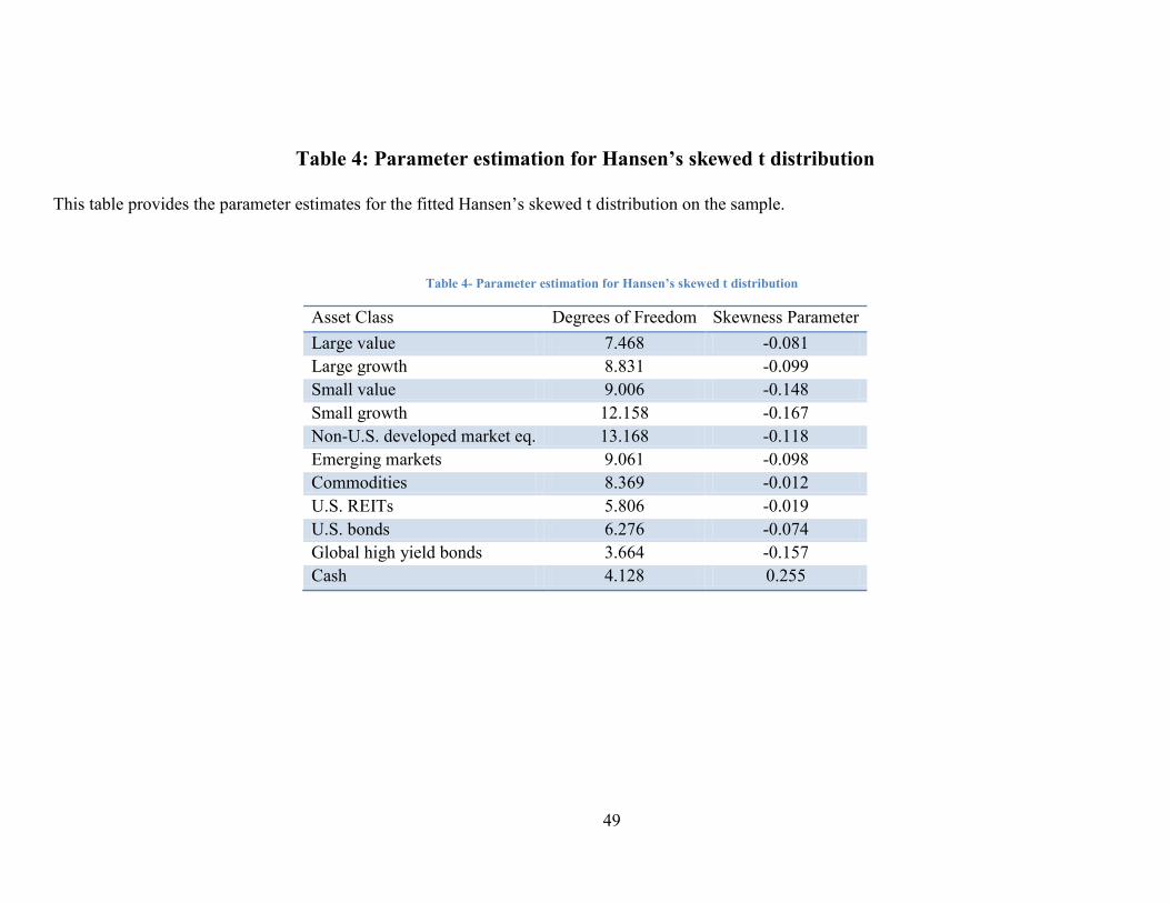
49

Table 4: Parameter estimation for Hansen’s skewed t distribution

This table provides the parameter estimates for the fitted Hansen’s skewed t distribution on the sample.

Table 4- Parameter estimation for Hansen’s skewed t distribution

Asset Class Degrees of Freedom Skewness Parameter

Large value 7.468 -0.081

Large growth 8.831 -0.099

Small value 9.006 -0.148

Small growth 12.158 -0.167

Non-U.S. developed market eq. 13.168 -0.118

Emerging markets 9.061 -0.098

Commodities 8.369 -0.012

U.S. REITs 5.806 -0.019

U.S. bonds 6.276 -0.074

Global high yield bonds 3.664 -0.157

Cash 4.128 0.255

50

Table 5: Parameter estimation for the copulas

This table provides the parameter estimates for the fitted copulas on the sample we use in this study.

Table 5- Parameter estimation for the copulas

Static t Copula Dynamic Normal Copula Dynamic t Copula

Parameter Estimate t-stat Estimate t-stat Estimate t-stat

Degrees of freedom 12.2452 22.6361 N/A 16.0584 18.3089

Alpha N/A 0.0105549 16.4593 0.01014 17.3286

Beta N/A 0.9871747 1042.326 0.98789 1189.9

Log Likelihood 13140.378 14345.405 14700.484

51

Table 6: Performance summary of CVaR optimizations with the historical means 2008/2009

This table provides a performance summary of our CVaR optimizations. The historical means are used as the expected means in our optimization

calculations. The performance measurement period is August 2008 to February 2009.

Table 6- Performance summary of CVaR optimizations with the historical means 2008/2009

CVaR Optimization

Expected Return Bootstrapping Static Normal Static t Dynamic Normal Dynamic t

6% -11.16% -10.40% -10.33% -10.56% -10.48%

7% -14.04% -12.09% -11.72% -10.44% -10.26%

8% -24.34% -22.82% -22.48% -18.81% -17.74%

9% -35.07% -34.05% -34.58% -30.09% -29.73%

52

Table 7: Performance summary of CVaR optimizations with the implied Black-Litterman means 2008/2009

This table provides a performance summary of our CVaR optimizations. The implied Black-Litterman means are used as the expected means our

optimization calculations. The performance measurement period is August 2008 to February 2009.

Table 7- Performance summary of CVaR optimizations with the implied Black-Litterman means 2008/2009

CVaR Optimization

Expected Return Bootstrapping Static Normal Static t Dynamic N Dynamic t

4% -32.96% -25.70% -25.76% -27.38% -23.39%

5% -40.71% -32.46% -31.78% -34.23% -30.05%

6% -48.34% -38.51% -38.99% -40.85% -37.14%

7% -55.44% -44.55% -46.75% -48.76% -44.35%

8% -64.42% -50.41% -50.16% -53.63% -55.54%

53

Table 8: Performance summary of CVaR optimizations with the historical means 2013

This table provides a performance summary of our CVaR optimizations. The historical means are used as the expected means in our optimization

calculations. The performance measurement period is December 31, 2012 to January 31, 2013.

Table 8- Performance summary of CVaR optimizations with the historical means 2013

CVaR Optimization

Expected Return Bootstrapping Static Normal Dynamic Normal Static t Dynamic t

6% 0.40% 0.28% 0.30% 0.33% 0.28%

7% 0.17% -0.33% -0.56% -0.22% -0.56%

8% 0.97% 0.38% 0.22% 0.34% 0.12%

9% 2.72% 2.50% 2.50% 2.50% 2.50%

54

Table 9: Performance summary of CVaR optimizations with the implied Black-Litterman means 2013

This table provides a performance summary of our CVaR optimizations. The implied Black-Litterman means are used as the expected means in our

optimization calculations. The performance measurement period is December 31, 2012 to January 31, 2013.

.

Table 9- Performance summary of CVaR optimizations with the implied Black-Litterman means 2013

CVaR Optimization

Expected Return Bootstrapping Static Normal Dynamic Normal Static t Dynamic t

4% 2.33% 2.25% 1.80% 2.23% 1.89%

5% 2.90% 2.80% 2.09% 2.77% 2.14%

6% 3.49% 3.27% 2.46% 3.18% 2.41%

7% 4.12% 3.75% 2.97% 3.67% 3.13%

8% 4.76% 4.55% 3.70% 4.43% 3.79%

55

Figure 1: Normal quantile-quantile plots

This figure shows the normal quantile-quantile plots for each sample used in our study.

-4 -3 -2 -1 0 1 2 3 4-0.06

-0.04

-0.02

0

0.02

0.04

0.06

Standard Normal Quantiles

Ru

sse

ll 2

000

Qu

an

tile

s

Russell 2000 Value

-4 -3 -2 -1 0 1 2 3 4-0.08

-0.06

-0.04

-0.02

0

0.02

0.04

0.06

Standard Normal Quantiles

Ru

sse

ll 1

000

Va

lue

Qu

an

tile

s

Russell 1000 Value

-4 -3 -2 -1 0 1 2 3 4-0.1

-0.08

-0.06

-0.04

-0.02

0

0.02

0.04

0.06

0.08

0.1

Standard Normal Quantiles

Ru

sse

ll 1

000

Gro

wth

Qu

an

tile

s

Russell 1000 Growth

-4 -3 -2 -1 0 1 2 3 4-0.1

-0.08

-0.06

-0.04

-0.02

0

0.02

0.04

0.06

0.08

Standard Normal Quantiles

Ru

sse

ll 2

000

Gro

wth

Qu

an

tile

s

Russell 2000 Growth

-4 -3 -2 -1 0 1 2 3 4-0.08

-0.06

-0.04

-0.02

0

0.02

0.04

0.06

Standard Normal Quantiles

MS

CI

Em

erg

ing

Ma

rke

ts Q

ua

nti

les

MSCI Emerging Markets Index

-4 -3 -2 -1 0 1 2 3 4-0.1

-0.08

-0.06

-0.04

-0.02

0

0.02

0.04

0.06

0.08

Standard Normal Quantiles

S&

P G

SC

I C

om

mo

dit

y I

nd

ex

Qu

an

tile

s S&P GSCI Commodity Index

-4 -3 -2 -1 0 1 2 3 4-0.08

-0.06

-0.04

-0.02

0

0.02

0.04

0.06

0.08

0.1

Standard Normal QuantilesFTS

E EP

RA

/NA

REI

T U

.S. I

nd

ex

Qu

an

tile

s FTSE EPRA/NAREIT U.S. Index

-4 -3 -2 -1 0 1 2 3 4-0.02

-0.015

-0.01

-0.005

0

0.005

0.01

0.015

Standard Normal Quantiles

Ba

rcla

ys

Ca

pit

al

U.S

. Ag

gre

ga

te B

on

d Q

ua

nti

les

Barclays Capital U.S. Aggregate Bond Index

-4 -3 -2 -1 0 1 2 3 4-0.06

-0.04

-0.02

0

0.02

0.04

0.06

Standard Normal Quantiles

MS

CI

Wo

rld

ex

US

A Q

ua

nti

les

MSCI World ex USA

Figure 1- Normal quantile-quantile plots

56

-4 -3 -2 -1 0 1 2 3

-0.025

-0.02

-0.015

-0.01

-0.005

0

0.005

0.01

0.015

0.02

Standard Normal Quantiles

Bo

fA M

L H

IGH

YIE

LD Q

ua

nti

les

BofA ML HIGH YIELD

57

Figure 2: Quantile-quantile plots based on Hansen skewed t

This figure shows the Hansen skewed t quantile-quantile plots for each index used in our sample.

Figure 2- Quantile-quantile plots based on Hansen skewed t

-8 -6 -4 -2 0 2 4 6-8

-6

-4

-2

0

2

4

6

Hansen's Skew t Quantiles

Ru

sse

ll 1

000

Va

lue

Qu

an

tile

s

Russell 1000 Value

-6 -4 -2 0 2 4

-8

-6

-4

-2

0

2

4

Hansen's Skew t Quantiles

Ru

sse

ll 1

000

Gro

wth

Qu

an

tile

s

Russell 1000 Growth

-8 -6 -4 -2 0 2 4 6-8

-6

-4

-2

0

2

4

6

Hansen's Skew t Quantiles

Ru

sse

ll 2

000

Va

lue

Qu

an

tile

s

Russell 2000 Value

-8 -6 -4 -2 0 2 4-8

-6

-4

-2

0

2

4

Hansen's Skew t Quantiles

Ru

sse

ll 2

000

Gro

wth

Qu

an

tile

s

Russell 2000 Growth

-5 -4 -3 -2 -1 0 1 2 3 4-6

-5

-4

-3

-2

-1

0

1

2

3

4

Hansen's Skew t Quantiles

MS

CI

Wo

rld

ex

US

A Q

ua

nti

les

MSCI World ex USA

-5 -4 -3 -2 -1 0 1 2 3 4 5-8

-6

-4

-2

0

2

4

6

Hansen's Skew t Quantiles

MS

CI

Em

erg

ing

Ma

rke

ts Q

ua

nti

les

MSCI Emerging Markets

-6 -4 -2 0 2 4 6-8

-6

-4

-2

0

2

4

6

Hansen's Skew t Quantiles

S&

P G

SC

I C

om

mo

dit

y I

nd

ex

Qu

an

tile

s

S&P GSCI Commodity Index

-10 -8 -6 -4 -2 0 2 4 6-10

-8

-6

-4

-2

0

2

4

6

Hansen's Skew t Quantiles

FTS

E EP

RA

/NA

REI

T U

.S. Q

ua

nti

les

FTSE EPRA/NAREIT U.S. Index

-8 -6 -4 -2 0 2 4 6-8

-6

-4

-2

0

2

4

6

Hansen's Skew t Quantiles

Ba

rcla

ys

Ca

pit

al

U.S

. Ag

gre

ga

te B

on

d Q

ua

nti

les

Barclays Capital U.S. Aggregate Bond Index

58

-20 -15 -10 -5 0 5

-20

-15

-10

-5

0

5

10

Hansen's Skew t Quantiles

BO

FA M

L H

IGH

YIE

LD Q

ua

nti

les

BofA ML HIGH YIELD

-6 -4 -2 0 2 4 6 8 10 12-8

-6

-4

-2

0

2

4

6

8

10

12

Hansen's Skew t Quantiles

Ca

sh Q

ua

nti

les

Cash

59

Figure 3: Performance summary of CVaR optimizations with the historical means 2008/2009

This graph shows the performance of our CVaR optimized portfolios in the year 2008 for the five different methods and the four levels of required

returns we used in this study. The historical means are used as the expected means in our optimization calculations. The performance measurement

period is August 31, 2008 to February 28, 2009. This figure clearly shows the improvement in portfolio performance when parametric models are

used.

Figure 3- : Performance summary of CVaR optimizations with the historical means 2008/2009

-39.00%

-36.00%

-33.00%

-30.00%

-27.00%

-24.00%

-21.00%

-18.00%

-15.00%

-12.00%

-9.00%

-6.00%

-3.00%

0.00%Bootsrapping Static Normal Static t Dynamic Normal Dynamic t

Rea

lized

Ret

urn

6%

7%

8%

9%

60

Figure 4: Performance summary of CVaR optimizations with the implied Black-Litterman means 2008/2009

This graph shows the performance of our CVaR optimized portfolios in the year 2008 for the five different methods and the five levels of required

returns we used in this study. The implied Black-Litterman means are used as the expected means in our optimization calculations. The performance

measurement period is August 31, 2008 to February 28, 2009. This figure clearly shows the improvement in portfolio performance when parametric

models are used.

Figure 4- Performance summary of CVaR optimizations with the implied Black-Litterman means 2008/2009

-70.00%

-60.00%

-50.00%

-40.00%

-30.00%

-20.00%

-10.00%

0.00%

Bootstrapping Static Normal Static t Dynamic N Dynamic t

Rea

lize

d R

eturn

4%

5%

6%

7%

8%

61

Figure 5: Performance summary of CVaR optimizations with the historical means 2013

This graph shows the performance of our CVaR optimized portfolios in the year 2013 for the five different methods and the four levels of required

returns we used in this study. Historical means are used as the expected means in our optimization calculations. The performance measurement

period is December 31, 2013 to January 31, 2013. This figure shows that our modeling approaches result in the almost same performance as a

bootstrapping approach.

-1.00%

0.00%

1.00%

2.00%

3.00%

4.00%

5.00%

6.00%

7.00%

8.00%

Bootstrapping Static Normal Dynamic Normal Static t Dynamic t

6%

7%

8%

9%

Figure 5- : Performance summary of CVaR optimizations with the historical means 2013

62

Figure 6: Performance summary of CVaR optimizations with the implied Black-Litterman means 2013

This graph shows the performance of our CVaR optimized portfolios in the year 2013 for the five different methods and the five levels of required

returns we used in this study. The implied Black-Litterman means are used as the expected means in our optimization calculations. The performance

measurement period is December 31, 2013 to January 31, 2013. This figure shows that our modeling approaches result in the almost same

performance as a bootstrapping approach.

0.00%

1.00%

2.00%

3.00%

4.00%

5.00%

6.00%

7.00%

8.00%

9.00%

10.00%

Bootstrapping Static Normal Dynamic Normal Static t Dynamic t

4%

5%

6%

7%

8%

Figure 6- : Performance summary of CVaR optimizations with the implied Black-Litterman means 2013

63

Figure 7: evolution of the dynamic correlation between U.S. bonds and U.S. equities

This figure provides the evolution of the dynamic correlation between U.S. bonds and U.S. equities. The line shows the average correlation over our

sample period. Both average and dynamic correlations are calculated using a t copula.

Figure 7- evolution of the dynamic correlation between U.S. bonds and U.S. equities

-0.8

-0.6

-0.4

-0.2

0

0.2

0.4

0.6

0.8

Dynamic

Correlation

Average Correlation: 0.0815

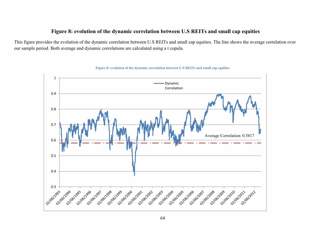
64

Figure 8: evolution of the dynamic correlation between U.S REITs and small cap equities

This figure provides the evolution of the dynamic correlation between U.S REITs and small cap equities. The line shows the average correlation over

our sample period. Both average and dynamic correlations are calculated using a t copula.

Figure 8- evolution of the dynamic correlation between U.S REITs and small cap equities

0.3

0.4

0.5

0.6

0.7

0.8

0.9

1

DynamicCorrelation

Average Correlation: 0.5817

65

Figure 9: evolution of the dynamic correlation between commodities and equities

This figure provides the evolution of the dynamic correlation between commodities and equities. The line shows the average correlation over the

period. Both average and dynamic correlations are calculated using a t copula.

Figure 9- evolution of the dynamic correlation between commodities and equities

-0.3

-0.2

-0.1

0

0.1

0.2

0.3

0.4

0.5

0.6

0.7Dynamic

Correlation

Average Correlation: 0.0123

66

Appendix

Table 1A: Bootstrapping Results August 2008 to February 2009 with Historical Means

This table presents detailed results for our mean-variance and CVaR optimization based on a bootstrapping approach. Historical means are

used as expected returns. The performance measurement period is August 2008 to February 2009.

No Asset Class Realized

Return

Expected Return

6%

Expected Return

7%

Expected Return

8%

Expected Return

9%

CVAR W MVO W CVAR W MVO W CVAR W MVO W CVAR W MVO W

1 Large value -45.80% -7.24% -4.41% -7.07% -6.39% 5.21% 5.80% 17.87% 17.76%

2 Large growth -40.47% 7.66% 4.93% 10.22% 9.22% 10.44% 9.41% 6.76% 6.72%

3 Small value -47.90% 8.75% 8.58% 29.88% 30.00% 30.00% 30.00% 30.00% 30.00%

4 Small growth -46.90% -7.88% -6.49% -21.79% -20.78% -27.92% -27.20% -28.99% -29.45%

5 Non-U.S. developed market

equities

-45.65% 2.98% 2.42% -5.22% -4.53% -13.00% -11.00% -21.14% -18.69%

6 Emerging markets -47.79% 0.08% 0.32% 5.18% 5.18% 12.52% 12.14% 19.55% 19.63%

7 Commodities -52.52% 3.81% 2.94% 8.15% 7.33% 17.22% 16.22% 26.64% 25.26%

8 U.S. REITs -62.40% 2.36% 1.73% -2.21% -2.23% 1.78% 3.23% 5.27% 7.68%

9 U.S. bonds 2.02% 29.63% 29.99% 29.67% 30.00% 30.00% 30.00% 30.00% 30.00%

10 Global high yield -22.96% 29.85% 29.99% 29.86% 30.00% 29.99% 30.00% 30.00% 30.00%

11 Cash 0.81% 30.00% 30.00% 23.34% 22.19% 3.76% 1.39% -15.95% -18.93%

Total -11.16% -10.96% -14.04% -14.40% -24.34% -25.66% -35.07% -36.76%

Difference -0.21% 0.35% 1.33% 1.69%

Std. Deviation 0.13% 0.13% 0.19% 0.18% 0.32% 0.31% 0.47% 0.46%

Value at Risk 0.19% 0.19% 0.28% 0.28% 0.49% 0.49% 0.73% 0.73%

CVaR 0.27% 0.29% 0.36% 0.40% 0.61% 0.67% 0.92% 1.01%

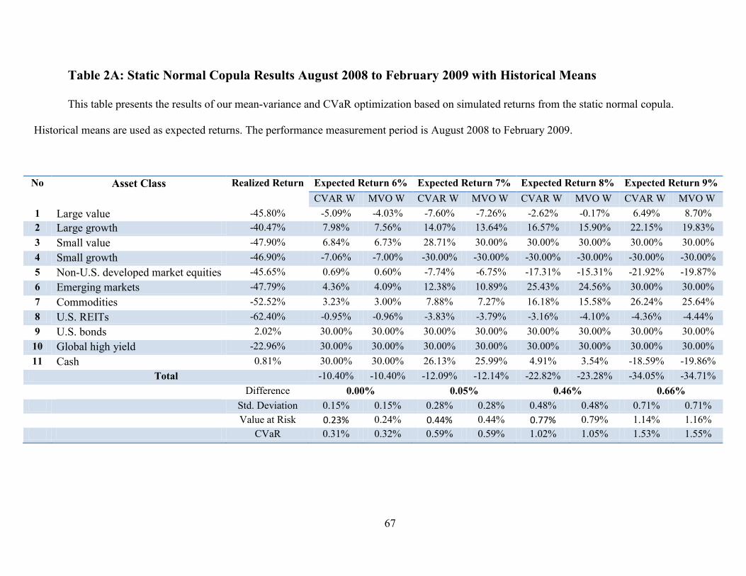
67

Table 2A: Static Normal Copula Results August 2008 to February 2009 with Historical Means

This table presents the results of our mean-variance and CVaR optimization based on simulated returns from the static normal copula.

Historical means are used as expected returns. The performance measurement period is August 2008 to February 2009.

No Asset Class Realized Return Expected Return 6% Expected Return 7% Expected Return 8% Expected Return 9%

CVAR W MVO W CVAR W MVO W CVAR W MVO W CVAR W MVO W

1 Large value -45.80% -5.09% -4.03% -7.60% -7.26% -2.62% -0.17% 6.49% 8.70%

2 Large growth -40.47% 7.98% 7.56% 14.07% 13.64% 16.57% 15.90% 22.15% 19.83%

3 Small value -47.90% 6.84% 6.73% 28.71% 30.00% 30.00% 30.00% 30.00% 30.00%

4 Small growth -46.90% -7.06% -7.00% -30.00% -30.00% -30.00% -30.00% -30.00% -30.00%

5 Non-U.S. developed market equities -45.65% 0.69% 0.60% -7.74% -6.75% -17.31% -15.31% -21.92% -19.87%

6 Emerging markets -47.79% 4.36% 4.09% 12.38% 10.89% 25.43% 24.56% 30.00% 30.00%

7 Commodities -52.52% 3.23% 3.00% 7.88% 7.27% 16.18% 15.58% 26.24% 25.64%

8 U.S. REITs -62.40% -0.95% -0.96% -3.83% -3.79% -3.16% -4.10% -4.36% -4.44%

9 U.S. bonds 2.02% 30.00% 30.00% 30.00% 30.00% 30.00% 30.00% 30.00% 30.00%

10 Global high yield -22.96% 30.00% 30.00% 30.00% 30.00% 30.00% 30.00% 30.00% 30.00%

11 Cash 0.81% 30.00% 30.00% 26.13% 25.99% 4.91% 3.54% -18.59% -19.86%

Total -10.40% -10.40% -12.09% -12.14% -22.82% -23.28% -34.05% -34.71%

Difference 0.00% 0.05% 0.46% 0.66%

Std. Deviation 0.15% 0.15% 0.28% 0.28% 0.48% 0.48% 0.71% 0.71%

Value at Risk 0.23% 0.24% 0.44% 0.44% 0.77% 0.79% 1.14% 1.16%

CVaR 0.31% 0.32% 0.59% 0.59% 1.02% 1.05% 1.53% 1.55%

68

Table 3A: Dynamic Normal Copula Results August 2008 to February 2009 with Historical Means

This table presents the results of our mean-variance and CVaR optimization based on simulated returns from a dynamic normal copula.

Historical means are used as expected returns. The performance measurement period is August 2008 to February 2009.

No Asset Class Realized Return Expected Return 6% Expected Return 7% Expected Return 8% Expected Return 9%

CVAR W MVO W CVAR W MVO W CVAR W MVO W CVAR W MVO W

1 Large value -45.80% -2.57% -2.46% -2.09% -1.48% 13.28% 14.93% 29.10% 30.00%

2 Large growth -40.47% 6.63% 7.01% 10.65% 10.79% 6.01% 5.34% 3.61% 3.49%

3 Small value -47.90% 7.01% 7.26% 30.00% 30.00% 30.00% 30.00% 30.00% 30.00%

4 Small growth -46.90% -5.16% -5.62% -30.00% -30.00% -30.00% -30.00% -30.00% -30.00%

5 Non-U.S. developed market equities -45.65% 0.41% 0.54% -11.88% -10.44% -26.69% -24.46% -30.00% -30.00%

6 Emerging markets -47.79% 0.78% 0.88% 10.92% 9.71% 25.23% 24.60% 30.00% 30.00%

7 Commodities -52.52% 2.95% 2.69% 6.15% 6.05% 13.75% 13.11% 23.04% 22.65%

8 U.S. REITs -62.40% -0.05% -0.30% -3.63% -3.47% -5.23% -5.43% -6.56% -6.79%

9 U.S. bonds 2.02% 30.00% 30.00% 30.00% 30.00% 30.00% 30.00% 30.00% 30.00%

10 Global high yield -22.96% 30.00% 30.00% 30.00% 30.00% 30.00% 30.00% 30.00% 30.00%

11 Cash 0.81% 30.00% 30.00% 29.89% 28.84% 13.65% 11.91% -9.19% -9.34%

Total -10.56% -10.48% -10.44% -10.92% -18.81% -19.57% -30.09% -30.10%

Difference -0.08% 0.47% 0.76% 0.02%

Std. Deviation 0.12% 0.13% 0.20% 0.20% 0.38% 0.39% 0.59% 0.59%

Value at Risk 0.18% 0.19% 0.30% 0.31% 0.61% 0.61% 0.94% 0.95%

CVaR 0.25% 0.26% 0.40% 0.42% 0.81% 0.82% 1.26% 1.27%

69

Table 4A: Static t Copula Results August 2008 to February 2009 with Historical Means

This table presents the results of our mean-variance and CVaR optimization based on simulated returns from a static t copula. Historical

means are used as expected returns. The performance measurement period is August 2008 to February 2009.

No Asset Class Realized Return Expected Return 6% Expected Return 7% Expected Return 8% Expected Return 9%

CVAR W MVO W CVAR W MVO W CVAR W MVO W CVAR W MVO W

1 Large value -45.80% -4.57% -4.27% -7.18% -6.58% -0.89% 0.92% 8.37% 10.42%

2 Large growth -40.47% 8.20% 7.88% 12.12% 12.73% 16.28% 14.60% 18.66% 18.07%

3 Small value -47.90% 6.94% 6.99% 30.00% 30.00% 30.00% 30.00% 30.00% 30.00%

4 Small growth -46.90% -7.65% -7.31% -30.00% -30.00% -30.00% -30.00% -30.00% -30.00%

5 Non-U.S. developed market equities -45.65% 1.09% 0.73% -7.06% -6.82% -16.47% -15.25% -18.92% -19.21%

6 Emerging markets -47.79% 4.02% 4.16% 11.66% 11.27% 24.13% 25.04% 30.00% 30.00%

7 Commodities -52.52% 3.15% 2.85% 7.83% 7.07% 16.58% 15.25% 26.56% 25.36%

8 U.S. REITs -62.40% -1.18% -1.03% -4.36% -3.78% -4.74% -4.16% -5.12% -4.62%

9 U.S. bonds 2.02% 30.00% 30.00% 30.00% 30.00% 30.00% 30.00% 30.00% 30.00%

10 Global high yield -22.96% 30.00% 30.00% 30.00% 30.00% 30.00% 30.00% 30.00% 30.00%

11 Cash 0.81% 30.00% 30.00% 26.98% 26.12% 5.11% 3.60% -19.56% -20.01%

Total -10.33% -10.37% -11.72% -12.13% -22.48% -23.30% -34.58% -34.82%

Difference 0.03% 0.41% 0.82% 0.24%

Std. Deviation 0.001491 0.001582 0.002852 0.002748 0.004872 0.004845 0.00724 0.007073

Value at Risk 0.22% 0.24% 0.45% 0.43% 0.78% 0.78% 1.17% 1.13%

CVaR 0.31% 0.34% 0.59% 0.61% 1.05% 1.06% 1.57% 1.58%

70

Table 5A: Dynamic t Copula Results August 2008 to February 2009 with Historical Means

This table presents the results of our mean-variance and CVaR optimization based on simulated returns from a dynamic t copula. Historical

means are used as expected returns. The performance measurement period is August 2008 to February 2009.

Dynamic t Copula Results August 2008 to February 2009 with Historical Means

No Asset Class Realized Return Expected Return 6% Expected Return 7% Expected Return 8% Expected Return 9%

CVAR W MVO W CVAR W MVO W CVAR W MVO W CVAR W MVO W

1 Large value -45.80% -3.33% -2.58% -2.05% -1.52% 17.18% 16.21% 30.00% 30.00%

2 Large growth -40.47% 7.89% 7.13% 11.64% 11.24% 3.09% 5.15% 4.63% 5.09%

3 Small value -47.90% 6.82% 7.28% 30.00% 30.00% 30.00% 30.00% 30.00% 30.00%

4 Small growth -46.90% -5.20% -5.61% -30.00% -30.00% -30.00% -30.00% -30.00% -30.00%

5 Non-U.S. developed market equities -45.65% -0.27% 0.46% -12.14% -11.27% -28.81% -26.24% -30.00% -30.00%

6 Emerging markets -47.79% 1.34% 1.06% 10.45% 10.11% 26.18% 25.50% 30.00% 30.00%

7 Commodities -52.52% 2.89% 2.64% 6.19% 5.91% 13.13% 12.65% 22.88% 22.42%

8 U.S. REITs -62.40% -0.15% -0.38% -4.09% -3.73% -6.53% -6.35% -8.33% -7.82%

9 U.S. bonds 2.02% 30.00% 30.00% 30.00% 30.00% 30.00% 30.00% 30.00% 30.00%

10 Global high yield -22.96% 30.00% 30.00% 30.00% 30.00% 30.00% 30.00% 30.00% 30.00%

11 Cash 0.81% 30.00% 30.00% 30.00% 29.26% 15.77% 13.08% -9.18% -9.68%

Total -10.48% -10.46% -10.26% -10.66% -17.74% -18.87% -29.73% -29.99%

Difference -0.02% 0.40% 1.12% 0.27%

Std. Deviation 0.122% 0.122% 0.197% 0.196% 0.382% 0.381% 0.595% 0.594%

Value at Risk 0.174% 0.174% 0.297% 0.294% 0.591% 0.589% 0.946% 0.940%

CVaR 0.248% 0.249% 0.401% 0.402% 0.798% 0.801% 1.263% 1.264%

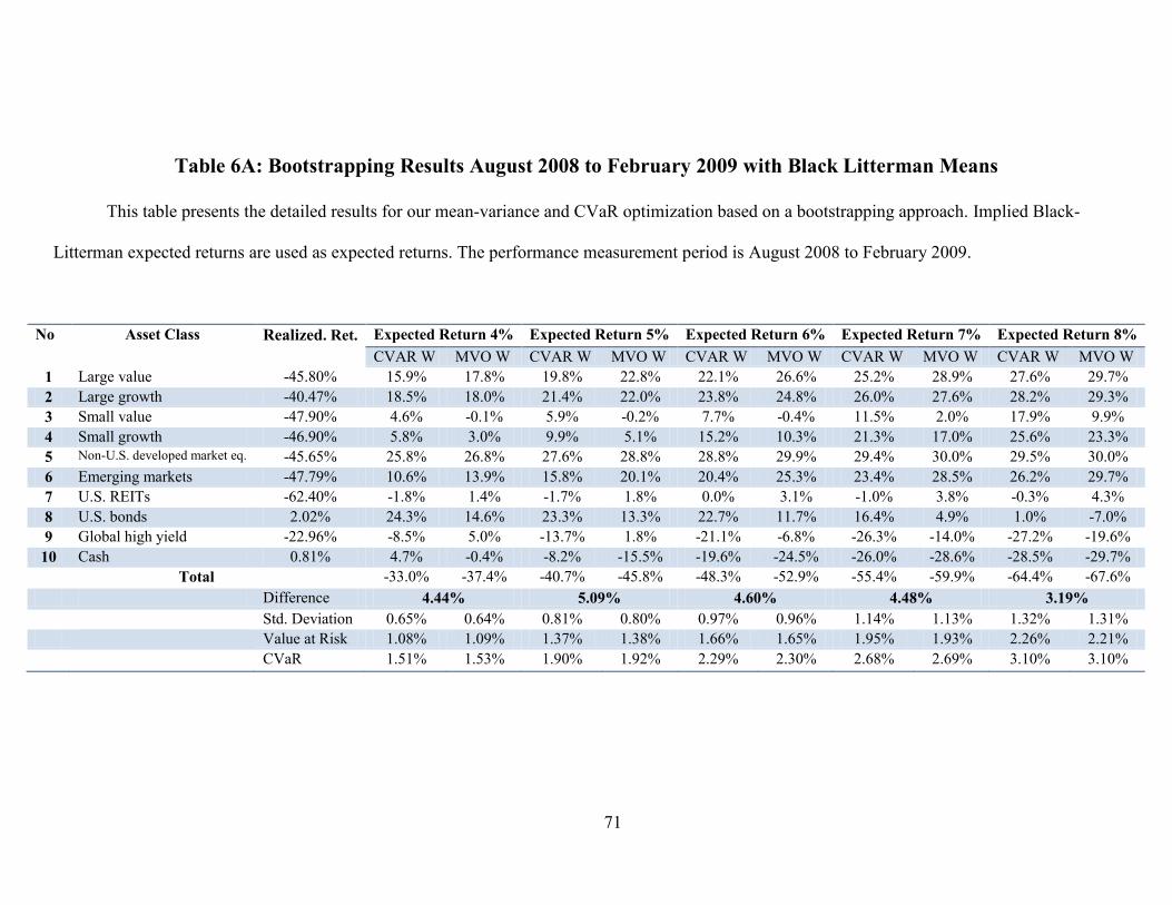
71

Table 6A: Bootstrapping Results August 2008 to February 2009 with Black Litterman Means

This table presents the detailed results for our mean-variance and CVaR optimization based on a bootstrapping approach. Implied Black-

Litterman expected returns are used as expected returns. The performance measurement period is August 2008 to February 2009.

No Asset Class Realized. Ret. Expected Return 4% Expected Return 5% Expected Return 6% Expected Return 7% Expected Return 8%

CVAR W MVO W CVAR W MVO W CVAR W MVO W CVAR W MVO W CVAR W MVO W

1 Large value -45.80% 15.9% 17.8% 19.8% 22.8% 22.1% 26.6% 25.2% 28.9% 27.6% 29.7%

2 Large growth -40.47% 18.5% 18.0% 21.4% 22.0% 23.8% 24.8% 26.0% 27.6% 28.2% 29.3%

3 Small value -47.90% 4.6% -0.1% 5.9% -0.2% 7.7% -0.4% 11.5% 2.0% 17.9% 9.9%

4 Small growth -46.90% 5.8% 3.0% 9.9% 5.1% 15.2% 10.3% 21.3% 17.0% 25.6% 23.3%

5 Non-U.S. developed market eq. -45.65% 25.8% 26.8% 27.6% 28.8% 28.8% 29.9% 29.4% 30.0% 29.5% 30.0%

6 Emerging markets -47.79% 10.6% 13.9% 15.8% 20.1% 20.4% 25.3% 23.4% 28.5% 26.2% 29.7%

7 U.S. REITs -62.40% -1.8% 1.4% -1.7% 1.8% 0.0% 3.1% -1.0% 3.8% -0.3% 4.3%

8 U.S. bonds 2.02% 24.3% 14.6% 23.3% 13.3% 22.7% 11.7% 16.4% 4.9% 1.0% -7.0%

9 Global high yield -22.96% -8.5% 5.0% -13.7% 1.8% -21.1% -6.8% -26.3% -14.0% -27.2% -19.6%

10 Cash 0.81% 4.7% -0.4% -8.2% -15.5% -19.6% -24.5% -26.0% -28.6% -28.5% -29.7%

Total -33.0% -37.4% -40.7% -45.8% -48.3% -52.9% -55.4% -59.9% -64.4% -67.6%

Difference 4.44% 5.09% 4.60% 4.48% 3.19%

Std. Deviation 0.65% 0.64% 0.81% 0.80% 0.97% 0.96% 1.14% 1.13% 1.32% 1.31%

Value at Risk 1.08% 1.09% 1.37% 1.38% 1.66% 1.65% 1.95% 1.93% 2.26% 2.21%

CVaR 1.51% 1.53% 1.90% 1.92% 2.29% 2.30% 2.68% 2.69% 3.10% 3.10%

72

Table 7A: Static Normal Copula Results August 2008 to February 2009 with Black Litterman Means

This table presents the detailed results for our mean-variance and CVaR optimization based on simulated returns from a static normal copula.

Implied Black-Litterman expected returns are used as expected returns. The performance measurement period is August 2008 to February 2009.

No Asset Class Realized Ret. Expected Return 4% Expected Return 5% Expected Return 6% Expected Return 7% Expected Return 8%

CVAR W MVO W CVAR W MVO W CVAR W MVO W CVAR W MVO W CVAR W MVO W

1 Large value -45.80% 12.09% 12.75% 15.15% 15.88% 17.82% 19.87% 21.62% 24.45% 26.68% 29.22%

2 Large growth -40.47% 12.60% 14.09% 15.71% 17.53% 21.41% 21.15% 26.10% 24.70% 27.66% 28.19%

3 Small value -47.90% 2.66E-02 1.26% 3.36% 1.57% 3.50% 1.88% 4.28% 2.35% 4.39% 2.89%

4 Small growth -46.90% -1.10% 1.30% -1.33% 1.60% -0.58% 2.39% -1.19% 2.92% 1.04% 3.33%

5 Non-U.S. developed market eq. -45.65% 24.69% 23.80% 30.00% 29.61% 30.00% 30.00% 30.00% 30.00% 30.00% 30.00%

6 Emerging markets -47.79% 9.88% 9.08% 12.60% 11.28% 18.56% 16.40% 24.45% 22.06% 29.25% 27.82%

7 U.S. REITs -62.40% 0.02133 0.41% 2.68% 0.50% 2.83% 0.69% 3.23% 0.95% 3.71% 1.25%

8 U.S. bonds 2.02% 0.201344 0.160903 24.48% 0.20252 30.00% 23.05% 30.00% 24.69% 30.00% 25.89%

9 Global high yield -22.96% -10.42% 0.82% -11.51% 1.22% -15.28% 7.56% -18.94% -2.13% -22.73% -18.59%

10 Cash 0.81% 27.33% 20.39% 8.86% 0.56% -8.25% -23.00% -19.54% -30.00% -30.00% -30.00%

Total -25.70% -27.92% -32.46% -34.96% -38.51% -43.10% -44.55% -47.78% -50.41% -50.96%

Difference 2.22% 2.50% 4.59% 3.23% 0.55%

Std. Deviation 0.57% 0.56% 0.70% 0.70% 0.84% 0.84% 0.98% 0.98% 1.12% 1.12%

Value at Risk 0.93% 0.94% 1.16% 1.17% 1.40% 1.41% 1.63% 1.64% 1.85% 1.87%

CVaR 1.24% 1.25% 1.55% 1.55% 1.85% 1.86% 2.16% 2.17% 2.47% 2.47%

73

Table 8A: Static t Copula Results August 2008 to February 2009 with Black Litterman Means

This table presents the detailed results for our mean-variance and CVaR optimization based on simulated returns from a static t copula.

Implied Black-Litterman expected returns are used as expected returns. The performance measurement period is August 2008 to February 2009.

N

o

Asset Class Realized

Ret.

Expected Return

4%

Expected Return

5%

Expected Return

6%

Expected Return

7%

Expected Return

8%

CVAR W MVO W CVAR W MVO W CVAR W MVO W CVAR W MVO W CVAR W MVO W

1 Large value -45.80% 12.72% 12.76% 15.66% 15.89% 19.62% 20.04% 24.24% 24.78% 29.48% 29.70%

2 Large growth -40.47% 12.83% 14.10% 16.35% 17.55% 19.54% 21.03% 22.98% 24.36% 24.75% 27.61%

3 Small value -47.90% 2.69% 1.27% 3.98% 1.57% 2.55% 1.93% 2.39% 2.50% 4.33% 3.13%

4 Small growth -46.90% -0.09% 1.30% -1.00% 1.60% 1.71% 2.38% 2.46% 2.87% 2.32% 3.23%

5 Non-U.S. developed market

eq. -45.65% 24.09% 23.82% 30.00% 29.63% 30.00% 30.00% 30.00% 30.00% 30.00% 30.00%

6 Emerging markets -47.79% 9.57% 9.08% 12.03% 11.28% 17.56% 16.37% 22.53% 22.02% 28.21% 27.77%

7 U.S. REITs -62.40% 1.02% 0.41% 1.21% 0.50% 2.02% 0.59% 2.54% 0.76% 2.66% 0.95%

8 U.S. bonds 2.02% 18.71% 16.09% 23.83% 20.26% 29.55% 23.06% 30.00% 25.21% 30.00% 27.14%

9 Global high yield -22.96% -9.22% 0.77% -13.36% 1.22% -12.02% 8.06% -7.14% -2.49% -21.75% -19.53%

10 Cash 0.81% 27.66% 20.40% 11.30% 0.47% -10.53% -23.47% -30.00% -30.00% -30.00% -30.00%

Total -25.76% -27.92% -31.78% -34.99% -38.99% -43.20% -46.75% -47.60% -50.16% -50.56%

Difference 2.17% 3.20% 4.20% 0.86% 0.40%

Std.

Deviation

0.564% 0.564% 0.702% 0.702% 0.840% 0.839% 0.979% 0.978% 1.119% 1.118%

Value at

Risk

0.916% 0.911% 1.141% 1.133% 1.372% 1.365% 1.602% 1.603% 1.828% 1.823%

CVaR 1.262% 1.262% 1.569% 1.571% 1.877% 1.879% 2.187% 2.189% 2.499% 2.501%

74

Table 9A: Dynamic Normal Copula Results August 2008 to February 2009 with Black Litterman Means

This table presents the detailed results for our mean-variance and CVaR optimization based on simulated returns from a dynamic normal

copula. Implied Black-Litterman expected returns are used as expected returns. The performance measurement period is August 2008 to February

2009.

No Asset Class Realized

Ret.

Expected Return

4%

Expected Return

5%

Expected Return

6%

Expected Return

7%

Expected Return

8%

CVAR W MVO W CVAR W MVO W CVAR W MVO W CVAR W MVO W CVAR W MVO W

1 Large value -45.80% 9.64% 13.05% 12.45% 16.21% 17.73% 20.91% 21.04% 26.25% 29.58% 30.00%

2 Large growth -40.47% 14.35% 14.30% 18.76% 17.87% 24.66% 21.66% 29.39% 25.82% 30.00% 30.00%

3 Small value -47.90% 2.76% 1.27% 3.73% 1.60% 4.17% 1.78% 5.67% 2.30% -0.76% 2.83%

4 Small growth -46.90% -3.23% 1.33% -4.71% 1.62% -5.96% 1.61% -7.79% 0.26% -1.14% 1.88%

5 Non-U.S. developed market

eq. -45.65% 26.30% 24.26% 30.00% 30.00% 30.00% 30.00% 30.00% 30.00% 30.00% 30.00%

6 Emerging markets -47.79% 9.55% 9.20% 14.00% 11.58% 19.76% 17.64% 26.12% 25.12% 30.00% 30.00%

7 U.S. REITs -62.40% 4.02% 0.43% 4.62% 0.50% 3.67% 0.26% 4.10% -0.08% 5.10% -0.36%

8 U.S. bonds 2.02% 12.04% 16.32% 15.41% 20.62% 18.06% 24.65% 22.99% 23.74% 17.12% 18.06%

9 Global high yield -22.96% -5.44% 1.11% -6.52% 1.44% -6.77% 10.68% -1.51% -3.40% -9.89% -12.41%

10 Cash 0.81% 30.00% 18.73% 12.27% -1.46% -5.32% -29.19% -30.00% -30.00% -30.00% -30.00%

Total -27.38% -28.51% -34.23% -35.65% -40.85% -44.43% -48.76% -48.33% -53.63% -52.95%

Difference 1.13% 1.42% 3.58% -0.43% -0.67%

Std.

Deviation

0.571% 0.569% 0.710% 0.708% 0.848% 0.846% 0.987% 0.985% 1.127% 1.125%

Value at

Risk

0.940% 0.944% 1.167% 1.174% 1.399% 1.400% 1.642% 1.630% 1.865% 1.858%

CVaR 1.261% 1.266% 1.569% 1.575% 1.878% 1.884% 2.188% 2.192% 2.499% 2.502%

75

Table 10A: Dynamic t Copula Results August 2008 to February 2009 with Black Litterman Means

This table presents the detailed results for our mean-variance and CVaR optimization based on simulated returns from a dynamic t copula.

Implied Black-Litterman expected returns are used as expected returns. The performance measurement period is August 2008 to February 2009.

No Asset Class Realized Ret. Expected Return 4% Expected Return 5% Expected Return 6% Expected Return 7% Expected Return 8%

CVAR W MVO W CVAR W MVO W CVAR W MVO W CVAR W MVO W CVAR W MVO W

1 Large value -45.80% 8.13% 14.25% 11.48% 17.59% 17.82% 21.48% 24.63% 27.09% 30.00% 30.00%

2 Large growth -40.47% 19.89% 11.07% 24.93% 13.51% 30.00% 22.25% 30.00% 26.62% 30.00% 30.00%

3 Small value -47.90% -0.96% -0.06% 0.17% -0.35% -0.41% 1.98% -1.29% 2.87% -7.31% 3.75%

4 Small growth -46.90% 1.21% 5.88% -0.95% 7.48% -3.90% 1.13% -1.14% -0.85% 9.17% 2.23%

5 Non-U.S. developed market eq. -45.65% 26.36% 23.51% 30.00% 29.15% 30.00% 30.00% 30.00% 30.00% 30.00% 30.00%

6 Emerging markets -47.79% 10.95% 10.17% 15.13% 12.77% 22.35% 18.22% 29.48% 25.84% 30.00% 30.00%

7 U.S. REITs -62.40% 2.42% 0.17% 2.63% 0.24% 3.06% 0.18% 2.48% -0.26% 3.48% -0.36%

8 U.S. bonds 2.02% 29.93% 28.87% 30.00% 30.00% 23.71% 24.37% 27.59% 23.63% 10.64% 15.87%

9 Global high yield -22.96% -27.93% -3.27% -29.43% -1.05% -30.00% 10.39% -29.61% -4.95% -5.98% -11.49%

10 Cash 0.81% 30.00% 9.41% 16.06% -9.35% 7.37% -30.00% -12.16% -30.00% -30.00% -30.00%

Total -23.39% -28.03% -30.05% -35.66% -37.14% -44.98% -44.35% -48.67% -55.54% -53.82%

Difference 4.63% 5.61% 7.84% 4.32% -1.72%

Std. Deviation 0.568% 0.566% 0.706% 0.704% 0.856% 0.853% 0.995% 0.993% 1.136% 1.135%

Value at Risk 0.93% 0.93% 1.15% 1.15% 1.39% 1.39% 1.61% 1.61% 1.86% 1.85%

CVaR 1.24% 1.24% 1.54% 1.55% 1.87% 1.87% 2.18% 2.18% 2.49% 2.49%

76

Table 11A: Bootstrapping results January 1, 2013 to January 31, 2013 with historical means

This table presents detailed results for our mean-variance and CVaR optimization based on a bootstrapping approach. Historical means are

used as expected returns. The performance measurement period is January 1, 2013 to January 31, 2013.

No Asset Class Realized Return Expected Return 6% Expected Return 7% Expected Return 8% Expected Return 9%

CVAR W MVO W CVAR W MVO W CVAR W MVO W CVAR W MVO W

1 Large value 6.32% -7.58% -5.53% -6.89% -6.87% 6.98% 4.33% 28.02% 26.84%

2 Large growth 4.21% 11.62% 9.06% 17.66% 17.92% 23.09% 24.75% 29.08% 28.95%

3 Small value 5.90% 12.98% 12.54% 29.96% 30.00% 30.00% 30.00% 30.00% 30.00%

4 Small growth 6.54% -12.26% -10.55% -23.66% -23.93% -28.38% -29.27% -27.99% -29.51%

5 Non-U.S. developed market eq. 4.82% 1.50% 0.83% -18.76% -19.54% -29.74% -29.99% -30.00% -30.00%

6 Emerging markets 1.25% 0.32% 1.14% 12.32% 13.72% 22.08% 25.25% 28.21% 29.30%

7 Commodities 4.45% 4.39% 3.57% 9.69% 8.39% 21.84% 19.47% 29.87% 29.90%

8 U.S. REITs 3.50% -0.91% -1.05% -6.44% -6.22% -10.16% -8.04% -18.16% -16.19%

9 U.S. bonds -0.74% 29.97% 30.00% 30.00% 30.00% 30.00% 30.00% 30.00% 30.00%

10 Global high yield 1.35% 29.97% 30.00% 30.00% 30.00% 30.00% 30.00% 30.00% 30.00%

11 Cash 0.01% 30.00% 30.00% 26.12% 26.53% 4.28% 3.48% -29.03% -29.30%

Total 0.40% 0.44% 0.17% 0.09% 0.97% 0.81% 2.72% 2.62%

Difference -0.04% 0.07% 0.16% 0.10%

Std. Deviation 0.161% 0.160% 0.256% 0.254% 0.468% 0.463% 0.752% 0.746%

Value at Risk 0.225% 0.220% 0.378% 0.377% 0.713% 0.696% 1.110% 1.105%

CVaR 0.32% 0.367% 0.49% 0.559% 0.95% 1.042% 1.69% 1.724%

77

Table 12A: Static Normal Copula results January 1, 2013 to January 31, 2013 with historical means

This table presents detailed results for our mean-variance and CVaR optimization based on simulated returns from a static normal copula.

Historical means are used as expected returns. The performance measurement period is January 1, 2013 to January 31, 2013.

No Asset Class Realized Return Expected Return 6% Expected Return 7% Expected Return 8% Expected Return 9%

CVAR W MVO W CVAR W MVO W CVAR W MVO W CVAR W MVO W

1 Large value 6.32% -5.89% -5.47% -10.82% -10.60% -9.61% -10.46% 22.37% 22.37%

2 Large growth 4.21% 5.18% 4.89% 14.72% 13.67% 23.12% 24.03% 30.00% 30.00%

3 Small value 5.90% 8.52% 9.38% 30.00% 30.00% 30.00% 30.00% 30.00% 30.00%

4 Small growth 6.54% -6.97% -7.25% -26.30% -24.95% -30.00% -30.00% -30.00% -30.00%

5 Non-U.S. developed market eq. 4.82% -2.34% -1.84% -22.50% -20.78% -30.00% -30.00% -30.00% -30.00%

6 Emerging markets 1.25% 5.59% 5.33% 18.35% 18.22% 30.00% 30.00% 30.00% 30.00%

7 Commodities 4.45% 4.18% 3.78% 9.11% 8.73% 20.15% 20.28% 30.00% 30.00%

8 U.S. REITs 3.50% 1.71% 1.17% -1.41% -0.99% 5.55% 5.23% -12.37% -12.37%

9 U.S. bonds -0.74% 30.00% 30.00% 30.00% 30.00% 30.00% 30.00% 30.00% 30.00%

10 Global high yield 1.35% 30.00% 30.00% 30.00% 30.00% 30.00% 30.00% 30.00% 30.00%

11 Cash 0.01% 30.00% 30.00% 28.85% 26.70% 0.79% 0.92% -30.00% -30.00%

Total 0.28% 0.31% -0.33% -0.19% 0.38% 0.36% 2.50% 2.50%

Difference -0.03% -0.14% 0.02% 0.00%

Std. Deviation 0.094% 0.094% 0.164% 0.163% 0.281% 0.281% 0.481% 0.481%

Value at Risk 0.135% 0.134% 0.247% 0.249% 0.437% 0.436% 0.762% 0.762%

CVaR 0.187% 0.187% 0.328% 0.329% 0.585% 0.585% 1.030% 1.030%

78

Table 13A: Dynamic Normal Copula results January 1, 2013 to January 31, 2013 with historical means

This table presents detailed results for our mean-variance and CVaR optimization based on simulated returns from a dynamic normal copula.

Historical means are used as expected returns. The performance measurement period is January 1, 2013 to January 31, 2013.

No Asset Class Realized Return Expected Return 6% Expected Return 7% Expected Return 8% Expected Return 9%

CVAR W MVO W CVAR W MVO W CVAR W MVO W CVAR W MVO W

1 Large value 6.32% 0.28% 0.73% -11.40% -10.99% -17.29% -17.66% 22.37% 22.37%

2 Large growth 4.21% 5.08% 4.57% 21.30% 19.70% 30.00% 30.00% 30.00% 30.00%

3 Small value 5.90% 6.43% 6.74% 30.00% 30.00% 30.00% 30.00% 30.00% 30.00%

4 Small growth 6.54% -7.66% -7.07% -30.00% -28.22% -30.00% -30.00% -30.00% -30.00%

5 Non-U.S. developed market eq. 4.82% -4.32% -4.26% -25.11% -25.40% -30.00% -30.00% -30.00% -30.00%

6 Emerging markets 1.25% 6.80% 6.50% 19.43% 19.48% 30.00% 30.00% 30.00% 30.00%

7 Commodities 4.45% 1.35% 1.01% 4.13% 3.84% 19.15% 18.93% 30.00% 30.00%

8 U.S. REITs 3.50% 2.04% 1.78% 1.66% 1.59% 7.94% 8.76% -12.37% -12.37%

9 U.S. bonds -0.74% 30.00% 30.00% 30.00% 30.00% 30.00% 30.00% 30.00% 30.00%

10 Global high yield 1.35% 30.00% 30.00% 30.00% 30.00% 30.00% 30.00% 30.00% 30.00%

11 Cash 0.01% 30.00% 30.00% 30.00% 30.00% 0.21% -0.03% -30.00% -30.00%

Total 0.30% 0.34% -0.56% -0.51% 0.22% 0.22% 2.50% 2.50%

Difference -0.04% -0.05% 0.00% 0.00%

Std. Deviation 0.066% 0.066% 0.100% 0.100% 0.245% 0.245% 0.491% 0.491%

Value at Risk 0.089% 0.088% 0.144% 0.144% 0.373% 0.371% 0.769% 0.769%

CVaR 0.1297% 0.1300% 0.2012% 0.2017% 0.5139% 0.5141% 1.0479% 1.0479%

79

Table 14A: Static t Copula results January 1, 2013 to January 31, 2013 with historical means

This table presents detailed results for our mean-variance and CVaR optimization based on simulated returns from a static t normal copula. Historical

means are used as expected returns. The performance measurement period is January 1, 2013 to January 31, 2013.

No Asset Class Realized Return Expected Return 6% Expected Return 7% Expected Return 8% Expected Return 9%

CVAR W MVO W CVAR W MVO W CVAR W MVO W CVAR W MVO W

1 Large value 6.32% -5.44% -6.03% -10.00% -11.00% -11.46% -11.39% 22.37% 22.37%

2 Large growth 4.21% 4.36% 5.16% 12.85% 13.78% 23.61% 24.76% 30.00% 30.00%

3 Small value 5.90% 9.91% 10.18% 30.00% 30.00% 30.00% 30.00% 30.00% 30.00%

4 Small growth 6.54% -7.20% -7.45% -25.02% -24.96% -30.00% -30.00% -30.00% -30.00%

5 Non-U.S. developed market eq. 4.82% -1.54% -1.39% -21.54% -20.30% -30.00% -30.00% -30.00% -30.00%

6 Emerging markets 1.25% 5.12% 5.12% 18.22% 18.40% 30.00% 30.00% 30.00% 30.00%

7 Commodities 4.45% 3.76% 3.52% 8.71% 8.67% 20.36% 20.41% 30.00% 30.00%

8 U.S. REITs 3.50% 1.03% 0.89% -0.60% -0.73% 6.89% 5.23% -12.37% -12.37%

9 U.S. bonds -0.74% 30.00% 30.00% 30.00% 30.00% 30.00% 30.00% 30.00% 30.00%

10 Global high yield 1.35% 30.00% 30.00% 30.00% 30.00% 30.00% 30.00% 30.00% 30.00%

11 Cash 0.01% 30.00% 30.00% 27.38% 26.14% 0.59% 0.99% -30.00% -30.00%

Total 0.33% 0.32% -0.22% -0.18% 0.34% 0.33% 2.50% 2.50%

Difference 0.01% -0.04% 0.00% 0.00%

Std. Deviation 0.092% 0.092% 0.158% 0.158% 0.277% 0.277% 0.477% 0.477%

Value at Risk 0.130% 0.131% 0.236% 0.237% 0.427% 0.423% 0.747% 0.747%

CVaR 0.190% 0.190% 0.328% 0.329% 0.589% 0.590% 1.045% 1.045%

80

Table 15A: Dynamic t Copula results January 1, 2013 to January 31, 2013 with historical means

This table presents detailed results for our mean-variance and CVaR optimization based on simulated returns from a dynamic t normal copula.

Historical means are used as expected returns. The performance measurement period is January 1, 2013 to January 31, 2013.

No Asset Class Realized Return Expected Return 6% Expected Return 7% Expected Return 8% Expected Return 9%

CVAR W MVO W CVAR W MVO W CVAR W MVO W CVAR W MVO W

1 Large value 6.32% -3.34% -3.66% -14.61% -14.14% -21.29% -19.01% 22.37% 22.37%

2 Large growth 4.21% 5.53% 6.00% 20.57% 19.73% 30.00% 30.00% 30.00% 30.00%

3 Small value 5.90% 7.01% 8.23% 30.00% 30.00% 30.00% 30.00% 30.00% 30.00%

4 Small growth 6.54% -6.81% -7.61% -29.13% -27.22% -30.00% -30.00% -30.00% -30.00%

5 Non-U.S. developed market eq. 4.82% -3.71% -2.98% -24.51% -24.80% -30.00% -30.00% -30.00% -30.00%

6 Emerging markets 1.25% 6.04% 5.69% 18.20% 19.06% 30.00% 30.00% 30.00% 30.00%

7 Commodities 4.45% 2.84% 2.36% 7.07% 6.08% 20.68% 20.10% 30.00% 30.00%

8 U.S. REITs 3.50% 2.43% 1.98% 2.41% 1.27% 10.48% 8.55% -12.37% -12.37%

9 U.S. bonds -0.74% 30.00% 30.00% 30.00% 30.00% 30.00% 30.00% 30.00% 30.00%

10 Global high yield 1.35% 30.00% 30.00% 30.00% 30.00% 30.00% 30.00% 30.00% 30.00%

11 Cash 0.01% 30.00% 30.00% 30.00% 30.00% 0.13% 0.36% -30.00% -30.00%

Total 0.28% 0.30% -0.56% -0.53% 0.12% 0.18% 2.50% 2.50%

Difference -0.01% -0.03% -0.05% 0.00%

Std. Deviation 0.079% 0.079% 0.125% 0.125% 0.258% 0.257% 0.496% 0.496%

Value at Risk 0.109% 0.109% 0.180% 0.179% 0.387% 0.387% 0.774% 0.774%

CVaR 0.159% 0.159% 0.251% 0.252% 0.535% 0.535% 1.062% 1.062%

81

Table 16A: Bootstrapping results January 1, 2013 to January 31, 2013 with Black-Litterman means

This table presents detailed results for our mean-variance and CVaR optimization based on simulated returns from a bootstrapping approach. Implied

Black-Litterman expected returns are used as expected returns. The performance measurement period is January 1, 2013 to January 31, 2013.

No Asset Class Realized

Return

Expected Return

4%

Expected Return

5%

Expected Return

6%

Expected Return

7%

Expected Return

8%

CVAR W MVO W CVAR W MVO W CVAR W MVO W CVAR W MVO W CVAR W MVO W

1 Large value 6.32% 9.72% 12.75% 12.46% 15.79% 15.07% 18.61% 17.49% 21.43% 20.25% 23.93%

2 Large growth 4.21% 16.63% 12.68% 18.81% 15.69% 20.52% 18.66% 22.16% 21.27% 23.48% 23.60%

3 Small value 5.90% -1.17% -3.29% -1.39% -3.70% -0.58% -3.53% 1.02% -3.24% 3.19% -2.34%

4 Small growth 6.54% 1.40% 2.16% 4.03% 2.84% 7.05% 3.61% 10.44% 5.19% 13.90% 7.82%

5 Non-U.S. developed market

eq. 4.82% 21.08% 19.33% 23.58% 23.03% 25.48% 25.66% 27.03% 27.63% 28.08% 28.89%

6 Emerging markets 1.25% 10.22% 10.59% 14.29% 14.15% 18.05% 18.25% 21.02% 22.25% 23.49% 25.44%

7 U.S. REITs 3.50% 1.46% 3.90% 1.77% 4.78% 1.86% 5.51% 1.85% 6.25% 2.02% 6.96%

8 U.S. bonds -0.74% 25.36% 18.03% 25.17% 18.91% 24.10% 18.05% 22.26% 14.84% 19.53% 9.70%

9 Global high yield 1.35% -1.03% 9.00% -3.91% 7.73% -6.88% 6.81% -9.62% 4.20% -13.29% 1.43%

10 Cash 0.01% 16.33% 14.86% 5.19% 0.77% -4.67% -11.63% -13.65% -19.82% -20.64% -25.44%

Total 2.33% 2.48% 2.90% 3.05% 3.49% 3.61% 4.12% 4.17% 4.76% 4.78%

Difference -0.14% -0.14% -0.11% -0.06% -0.02%

Std. Deviation 0.577% 0.578% 0.718% 0.719% 0.860% 0.860% 1.002% 1.000% 1.145% 1.142%

Value at Risk 0.887% 0.880% 1.122% 1.098% 1.344% 1.322% 1.568% 1.541% 1.789% 1.762%

CVaR 1.395% 1.414% 1.739% 1.760% 2.084% 2.105% 2.429% 2.449% 2.777% 2.796%

82

Table 17A: Static normal copula results January 1, 2013 to January 31, 2013 with Black-Litterman means

This table presents detailed results for our mean-variance and CVaR optimization based on simulated returns from a static normal copula. Implied

Black-Litterman expected returns are used as expected returns. The performance measurement period is January 1, 2013 to January 31, 2013.

No Asset Class Realized

Return

Expected Return

4%

Expected Return

5%

Expected Return

6%

Expected Return

7%

Expected Return

8%

CVAR W MVO W CVAR W MVO W CVAR W MVO W CVAR W MVO W CVAR W MVO W

1 Large value 6.32% 3.33% 1.69% 3.53% 2.07% 2.26% 0.81% 4.63% 1.47% 10.41% 5.34%

2 Large growth 4.21% -2.25% -1.21% -2.83% -1.47% -1.84% -0.26% 0.53% 3.52% 6.06% 10.62%

3 Small value 5.90% -26.21% -24.24% -30.00% -30.00% -30.00% -30.00% -30.00% -30.00% -28.22% -27.99%

4 Small growth 6.54% 23.82% 23.12% 27.82% 28.65% 29.76% 30.00% 30.00% 30.00% 30.00% 30.00%

5 Non-U.S. developed market

eq. 4.82% 21.83% 21.24% 27.65% 26.45% 30.00% 30.00% 30.00% 30.00% 30.00% 30.00%

6 Emerging markets 1.25% 14.54% 14.78% 18.04% 18.41% 23.19% 23.87% 30.00% 30.00% 30.00% 30.00%

7 U.S. REITs 3.50% 19.02% 18.30% 23.50% 22.74% 27.78% 26.68% 30.00% 30.00% 30.00% 30.00%

8 U.S. bonds -0.74% 8.54% 7.97% 10.68% 10.03% 11.20% 12.97% 4.84% 5.01% -8.25% -7.98%

9 Global high yield 1.35% 21.12% 24.65% 25.44% 30.00% 30.00% 30.00% 30.00% 30.00% 30.00% 30.00%

10 Cash 0.01% 16.27% 13.70% -3.82% -6.88% -22.35% -24.07% -30.00% -30.00% -30.00% -30.00%

Total 2.25% 2.26% 2.80% 2.81% 3.27% 3.22% 3.75% 3.67% 4.55% 4.43%

Difference -0.01% -0.01% 0.05% 0.08% 0.12%

Std. Deviation 0.263% 0.263% 0.327% 0.327% 0.391% 0.391% 0.457% 0.456% 0.531% 0.530%

Value at Risk 0.430% 0.430% 0.534% 0.535% 0.636% 0.636% 0.740% 0.740% 0.865% 0.867%

CVaR 0.564% 0.564% 0.701% 0.701% 0.839% 0.839% 0.980% 0.981% 1.140% 1.142%

83

Table 18A: Static t copula results January 1, 2013 to January 31, 2013 with Black-Litterman means

This table presents detailed results for our mean-variance and CVaR optimization based on simulated returns from a static t copula. Implied Black-

Litterman expected returns are used as expected returns. The performance measurement period is January 1, 2013 to January 31, 2013.

No Asset Class Realized

Return

Expected Return

4%

Expected Return

5%

Expected Return

6%

Expected Return

7%

Expected Return

8%

CVAR W MVO W CVAR W MVO W CVAR W MVO W CVAR W MVO W CVAR W MVO W

1 Large value 6.32% 1.63% -2.26% 1.95% -2.99% 0.59% -5.11% 1.28% -3.09% 5.25% -3.09%

2 Large growth 4.21% -1.40% 0.75% -1.47% 1.53% 0.05% 4.66% 3.69% 17.18% 10.37% 17.18%

3 Small value 5.90% -24.58% -24.52% -30.00% -29.70% -30.00% -30.00% -30.00% -26.53% -27.63% -26.53%

4 Small growth 6.54% 24.65% 24.97% 30.00% 30.00% 30.00% 30.00% 30.00% 30.00% 30.00% 30.00%

5 Non-U.S. developed market

eq. 4.82% 22.25% 21.03% 27.88% 26.61% 30.00% 30.00% 30.00% 30.00% 30.00% 30.00%

6 Emerging markets 1.25% 14.85% 15.30% 18.30% 19.37% 24.90% 25.36% 30.00% 30.00% 30.00% 30.00%

7 U.S. REITs 3.50% 16.90% 17.38% 20.92% 21.71% 25.67% 26.07% 30.00% 30.00% 30.00% 30.00%

8 U.S. bonds -0.74% 9.94% 10.63% 12.50% 14.62% 14.22% 18.14% 5.02% -7.56% -7.99% -7.56%

9 Global high yield 1.35% 17.98% 30.00% 22.87% 30.00% 30.00% 30.00% 30.00% 30.00% 30.00% 30.00%

10 Cash 0.01% 17.79% 6.72% -2.93% -11.15% -25.42% -30.00% -30.00% -30.00% -30.00% -30.00%

Total 2.23% 2.22% 2.78% 2.67% 3.19% 3.01% 3.67% 4.26% 4.44% 4.26%

Difference 0.02% 0.11% 0.18% -0.59% 0.18%

Std. Deviation 0.264% 0.263% 0.328% 0.327% 0.392% 0.391% 0.459% 0.534% 0.535% 0.534%

Value at Risk 0.439% 0.440% 0.546% 0.548% 0.653% 0.655% 0.761% 0.878% 0.875% 0.878%

CVaR 0.581% 0.595% 0.723% 0.739% 0.865% 0.884% 1.011% 1.200% 1.175% 1.200%

84

Table 19A: Dynamic normal copula results January 1, 2013 to January 31, 2013 with Black-Litterman means

This table presents detailed results for our mean-variance and CVaR optimization based on simulated returns from a dynamic normal copula. Implied

Black-Litterman expected returns are used as expected returns. The performance measurement period is January 1, 2013 to January 31, 2013.

No Asset Class Realized

Return

Expected Return

4%

Expected Return

5%

Expected Return

6%

Expected Return

7%

Expected Return

8%

CVAR W MVO W CVAR W MVO W CVAR W MVO W CVAR W MVO W CVAR W MVO W

1 Large value 6.32% 6.16% 6.60% 3.46% 3.01% 1.60% 0.44% 2.26% -0.32% 3.66% -0.75%

2 Large growth 4.21% -4.05% -5.70% -1.38% -2.43% 4.72% 2.04% 9.15% 8.20% 18.73% 16.43%

3 Small value 5.90% -30.00% -30.00% -30.00% -30.00% -30.00% -29.79% -30.00% -27.08% -30.00% -23.34%

4 Small growth 6.54% 30.00% 30.00% 30.00% 30.00% 30.00% 30.00% 30.00% 30.00% 30.00% 30.00%

5 Non-U.S. developed market

eq. 4.82% 23.75% 23.11% 29.78% 28.75% 30.00% 30.00% 30.00% 30.00% 30.00% 30.00%

6 Emerging markets 1.25% 19.06% 19.22% 25.00% 25.37% 30.00% 30.00% 30.00% 30.00% 30.00% 30.00%

7 U.S. REITs 3.50% 13.29% 14.98% 17.56% 19.65% 21.89% 25.60% 30.00% 30.00% 30.00% 30.00%

8 U.S. bonds -0.74% 30.00% 30.00% 30.00% 30.00% 30.00% 30.00% 30.00% 30.00% 30.00% 30.00%

9 Global high yield 1.35% -18.22% -18.22% -30.00% -30.00% -30.00% -30.00% -30.00% -24.68% -12.39% -12.35%

10 Cash 0.01% 30.00% 30.00% 25.58% 25.65% 11.78% 11.71% -1.41% -6.12% -30.00% -30.00%

Total 1.80% 1.79% 2.09% 2.05% 2.46% 2.41% 2.97% 3.01% 3.70% 3.71%

Difference 0.01% 0.04% 0.04% -0.04% -0.02%

Std. Deviation 0.247% 0.246% 0.315% 0.314% 0.385% 0.384% 0.459% 0.459% 0.540% 0.540%

Value at Risk 0.400% 0.398% 0.507% 0.510% 0.625% 0.622% 0.746% 0.747% 0.874% 0.871%

CVaR 0.528% 0.529% 0.674% 0.674% 0.824% 0.825% 0.989% 0.990% 1.166% 1.167%

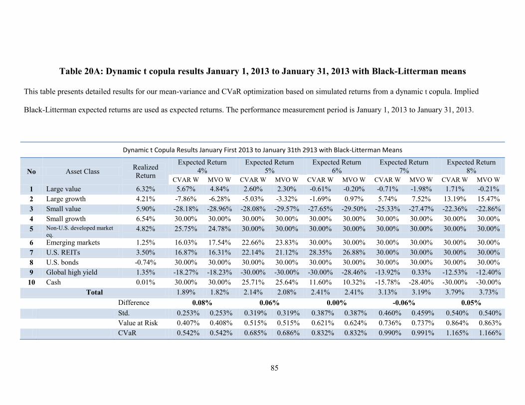
85

Table 20A: Dynamic t copula results January 1, 2013 to January 31, 2013 with Black-Litterman means

This table presents detailed results for our mean-variance and CVaR optimization based on simulated returns from a dynamic t copula. Implied

Black-Litterman expected returns are used as expected returns. The performance measurement period is January 1, 2013 to January 31, 2013.

Dynamic t Copula Results January First 2013 to January 31th 2913 with Black-Litterman Means

No Asset Class Realized

Return

Expected Return

4%

Expected Return

5%

Expected Return

6%

Expected Return

7%

Expected Return

8%

CVAR W MVO W CVAR W MVO W CVAR W MVO W CVAR W MVO W CVAR W MVO W

1 Large value 6.32% 5.67% 4.84% 2.60% 2.30% -0.61% -0.20% -0.71% -1.98% 1.71% -0.21%

2 Large growth 4.21% -7.86% -6.28% -5.03% -3.32% -1.69% 0.97% 5.74% 7.52% 13.19% 15.47%

3 Small value 5.90% -28.18% -28.96% -28.08% -29.57% -27.65% -29.50% -25.33% -27.47% -22.36% -22.86%

4 Small growth 6.54% 30.00% 30.00% 30.00% 30.00% 30.00% 30.00% 30.00% 30.00% 30.00% 30.00%

5 Non-U.S. developed market

eq. 4.82% 25.75% 24.78% 30.00% 30.00% 30.00% 30.00% 30.00% 30.00% 30.00% 30.00%

6 Emerging markets 1.25% 16.03% 17.54% 22.66% 23.83% 30.00% 30.00% 30.00% 30.00% 30.00% 30.00%

7 U.S. REITs 3.50% 16.87% 16.31% 22.14% 21.12% 28.35% 26.88% 30.00% 30.00% 30.00% 30.00%

8 U.S. bonds -0.74% 30.00% 30.00% 30.00% 30.00% 30.00% 30.00% 30.00% 30.00% 30.00% 30.00%

9 Global high yield 1.35% -18.27% -18.23% -30.00% -30.00% -30.00% -28.46% -13.92% 0.33% -12.53% -12.40%

10 Cash 0.01% 30.00% 30.00% 25.71% 25.64% 11.60% 10.32% -15.78% -28.40% -30.00% -30.00%

Total 1.89% 1.82% 2.14% 2.08% 2.41% 2.41% 3.13% 3.19% 3.79% 3.73%

Difference 0.08% 0.06% 0.00% -0.06% 0.05%

Std. 0.253% 0.253% 0.319% 0.319% 0.387% 0.387% 0.460% 0.459% 0.540% 0.540%

Value at Risk 0.407% 0.408% 0.515% 0.515% 0.621% 0.624% 0.736% 0.737% 0.864% 0.863%

CVaR 0.542% 0.542% 0.685% 0.686% 0.832% 0.832% 0.990% 0.991% 1.165% 1.166%

86

Figure 1A: Time series Plots of the data

This figure shows the time series plots for each index represented in our sample.

-15.00%-10.00%

-5.00%0.00%5.00%

10.00%15.00%

Jun

e-0

2-9

3

Jun

e-0

2-9

5

Jun

e-0

2-9

7

Jun

e-0

2-9

9

Jun

e-0

2-0

1

Jun

e-0

2-0

3

Jun

e-0

2-0

5

Jun

e-0

2-0

7

Jun

e-0

2-0

9

Jun

e-0

2-1

1

Jun

e-0

2-1

3

Russel 1000 Growth

-15.00%-10.00%

-5.00%0.00%5.00%

10.00%15.00%

Jun

e-0

2-9

3

Jun

e-0

2-9

5

Jun

e-0

2-9

7

Jun

e-0

2-9

9

Jun

e-0

2-0

1

Jun

e-0

2-0

3

Jun

e-0

2-0

5

Jun

e-0

2-0

7

Jun

e-0

2-0

9

Jun

e-0

2-1

1

Jun

e-0

2-1

3

Russell 1000 Value

-15.00%-10.00%

-5.00%0.00%5.00%

10.00%

Jun

e-0

2-9

3

Jun

e-0

2-9

5

Jun

e-0

2-9

7

Jun

e-0

2-9

9

Jun

e-0

2-0

1

Jun

e-0

2-0

3

Jun

e-0

2-0

5

Jun

e-0

2-0

7

Jun

e-0

2-0

9

Jun

e-0

2-1

1

Jun

e-0

2-1

3

Russel 2000 Value

-15.00%-10.00%

-5.00%0.00%5.00%

10.00%15.00%

Jun

e-0

2-9

3

Jun

e-0

2-9

5

Jun

e-0

2-9

7

Jun

e-0

2-9

9

Jun

e-0

2-0

1

Jun

e-0

2-0

3

Jun

e-0

2-0

5

Jun

e-0

2-0

7

Jun

e-0

2-0

9

Jun

e-0

2-1

1

Jun

e-0

2-1

3

Russel 2000 Growth

-10.00%

-5.00%

0.00%

5.00%

10.00%Ju

ne

-02

-93

Jun

e-0

2-9

5

Jun

e-0

2-9

7

Jun

e-0

2-9

9

Jun

e-0

2-0

1

Jun

e-0

2-0

3

Jun

e-0

2-0

5

Jun

e-0

2-0

7

Jun

e-0

2-0

9

Jun

e-0

2-1

1

Jun

e-0

2-1

3

MSCI World ex U.S.A.

-15.00%-10.00%

-5.00%0.00%5.00%

10.00%15.00%

Jun

e-0

2-9

3

Jun

e-0

2-9

5

Jun

e-0

2-9

7

Jun

e-0

2-9

9

Jun

e-0

2-0

1

Jun

e-0

2-0

3

Jun

e-0

2-0

5

Jun

e-0

2-0

7

Jun

e-0

2-0

9

Jun

e-0

2-1

1

Jun

e-0

2-1

3

MSCI World EM

-10.00%

-5.00%

0.00%

5.00%

10.00%

Jun

e-0

2-9

3

Jun

e-0

2-9

5

Jun

e-0

2-9

7

Jun

e-0

2-9

9

Jun

e-0

2-0

1

Jun

e-0

2-0

3

Jun

e-0

2-0

5

Jun

e-0

2-0

7

Jun

e-0

2-0

9

Jun

e-0

2-1

1

Jun

e-0

2-1

3

S&P GSCI Commodity Index

-40.00%

-20.00%

0.00%

20.00%

40.00%

Jun

e-0

2-9

3

Jun

e-0

2-9

5

Jun

e-0

2-9

7

Jun

e-0

2-9

9

Jun

e-0

2-0

1

Jun

e-0

2-0

3

Jun

e-0

2-0

5

Jun

e-0

2-0

7

Jun

e-0

2-0

9

Jun

e-0

2-1

1

Jun

e-0

2-1

3

U.S. REIT

-3.00%-2.00%-1.00%0.00%1.00%2.00%

Jun

e-0

2-9

3

Jun

e-0

2-9

5

Jun

e-0

2-9

7

Jun

e-0

2-9

9

Jun

e-0

2-0

1

Jun

e-0

2-0

3

Jun

e-0

2-0

5

Jun

e-0

2-0

7

Jun

e-0

2-0

9

Jun

e-0

2-1

1

Jun

e-0

2-1

3

Barclays Capital U.S. Aggregate Index

87

-6.00%

-4.00%

-2.00%

0.00%

2.00%

4.00%

ML High Yield Bond Index

-0.30%-0.20%-0.10%0.00%0.10%0.20%

Jun

e-0

2-9

3

Jun

e-0

2-9

5

Jun

e-0

2-9

7

Jun

e-0

2-9

9

Jun

e-0

2-0

1

Jun

e-0

2-0

3

Jun

e-0

2-0

5

Jun

e-0

2-0

7

Jun

e-0

2-0

9

Jun

e-0

2-1

1

Jun

e-0

2-1

3

Cash