Conditional Random Fields as Recurrent Neural Networks

Shuai Zheng∗1, Sadeep Jayasumana*1, Bernardino Romera-Paredes1, Vibhav Vineet†1,2, Zhizhong Su3,Dalong Du3, Chang Huang3, and Philip H. S. Torr1

1University of Oxford 2Stanford University 3Baidu Institute of Deep Learning

Abstract

Pixel-level labelling tasks, such as semantic segmenta-tion, play a central role in image understanding. Recent ap-proaches have attempted to harness the capabilities of deeplearning techniques for image recognition to tackle pixel-level labelling tasks. One central issue in this methodologyis the limited capacity of deep learning techniques to de-lineate visual objects. To solve this problem, we introducea new form of convolutional neural network that combinesthe strengths of Convolutional Neural Networks (CNNs)and Conditional Random Fields (CRFs)-based probabilisticgraphical modelling. To this end, we formulate mean-fieldapproximate inference for the Conditional Random Fieldswith Gaussian pairwise potentials as Recurrent Neural Net-works. This network, called CRF-RNN, is then plugged inas a part of a CNN to obtain a deep network that has de-sirable properties of both CNNs and CRFs. Importantly,our system fully integrates CRF modelling with CNNs, mak-ing it possible to train the whole deep network end-to-endwith the usual back-propagation algorithm, avoiding offlinepost-processing methods for object delineation.

We apply the proposed method to the problem of seman-tic image segmentation, obtaining top results on the chal-lenging Pascal VOC 2012 segmentation benchmark.

1. Introduction

Low-level computer vision problems such as semanticimage segmentation or depth estimation often involve as-signing a label to each pixel in an image. While the featurerepresentation used to classify individual pixels plays an im-portant role in this task, it is similarly important to considerfactors such as image edges, appearance consistency andspatial consistency while assigning labels in order to obtainaccurate and precise results.

Designing a strong feature representation is a key chal-

∗Authors contributed equally.†Work conducted while authors at the University of Oxford.

lenge in pixel-level labelling problems. Work on this topicincludes: TextonBoost [52], TextonForest [51], and Ran-dom Forest-based classifiers [50]. Recently, superviseddeep learning approaches such as large-scale deep Convolu-tional Neural Networks (CNNs) have been immensely suc-cessful in many high-level computer vision tasks such asimage recognition [31] and object detection [20]. This mo-tivates exploring the use of CNNs for pixel-level labellingproblems. The key insight is to learn a strong feature rep-resentation end-to-end for the pixel-level labelling task in-stead of hand-crafting features with heuristic parameter tun-ing. In fact, a number of recent approaches including theparticularly interesting works FCN [37] and DeepLab [10]have shown a significant accuracy boost by adapting state-of-the-art CNN based image classifiers to the semantic seg-mentation problem.

However, there are significant challenges in adaptingCNNs designed for high level computer vision tasks such asobject recognition to pixel-level labelling tasks. Firstly, tra-ditional CNNs have convolutional filters with large recep-tive fields and hence produce coarse outputs when restruc-tured to produce pixel-level labels [37]. Presence of max-pooling layers in CNNs further reduces the chance of get-ting a fine segmentation output [10]. This, for instance, canresult in non-sharp boundaries and blob-like shapes in se-mantic segmentation tasks. Secondly, CNNs lack smooth-ness constraints that encourage label agreement betweensimilar pixels, and spatial and appearance consistency of thelabelling output. Lack of such smoothness constraints canresult in poor object delineation and small spurious regionsin the segmentation output [59, 58, 32, 39].

On a separate track to the progress of deep learningtechniques, probabilistic graphical models have been devel-oped as effective methods to enhance the accuracy of pixel-level labelling tasks. In particular, Markov Random Fields(MRFs) and its variant Conditional Random Fields (CRFs)have observed widespread success in this area [32, 29] andhave become one of the most successful graphical modelsused in computer vision. The key idea of CRF inferencefor semantic labelling is to formulate the label assignment

1

problem as a probabilistic inference problem that incor-porates assumptions such as the label agreement betweensimilar pixels. CRF inference is able to refine weak andcoarse pixel-level label predictions to produce sharp bound-aries and fine-grained segmentations. Therefore, intuitively,CRFs can be used to overcome the drawbacks in utilizingCNNs for pixel-level labelling tasks.

One way to utilize CRFs to improve the semantic la-belling results produced by a CNN is to apply CRF infer-ence as a post-processing step disconnected from the train-ing of the CNN [10]. Arguably, this does not fully harnessthe strength of CRFs since it is not integrated with the deepnetwork. In this setup, the deep network is unaware of theCRF during the training phase.

In this paper, we propose an end-to-end deep learn-ing solution for the pixel-level semantic image segmenta-tion problem. Our formulation combines the strengths ofboth CNNs and CRF based graphical models in one uni-fied framework. More specifically, we formulate mean-fieldapproximate inference for the dense CRF with Gaussianpairwise potentials as a Recurrent Neural Network (RNN)which can refine coarse outputs from a traditional CNN inthe forward pass, while passing error differentials back tothe CNN during training. Importantly, with our formula-tion, the whole deep network, which comprises a traditionalCNN and an RNN for CRF inference, can be trained end-to-end utilizing the usual back-propagation algorithm.

Arguably, when properly trained, the proposed networkshould outperform a system where CRF inference is appliedas a post-processing method on independent pixel-level pre-dictions produced by a pre-trained CNN. Our experimentalevaluation confirms that this indeed is the case. We evaluatethe performance of our network on the popular Pascal VOC2012 benchmark, achieving a new state-of-the-art accuracyof 74.7%.

2. Related WorkIn this section we review approaches that make use of

deep learning and CNNs for low-level computer visiontasks, with a focus on semantic image segmentation. A widevariety of approaches have been proposed to tackle the se-mantic image segmentation task using deep learning. Theseapproaches can be categorized into two main strategies.

The first strategy is based on utilizing separate mecha-nisms for feature extraction, and image segmentation ex-ploiting the edges of the image [2, 38]. One representativeinstance of this scheme is the application of a CNN for theextraction of meaningful features, and using superpixels toaccount for the structural pattern of the image. Two repre-sentative examples are [19, 38], where the authors first ob-tained superpixels from the image and then used a featureextraction process on each of them. The main disadvantageof this strategy is that errors in the initial proposals (e.g:

super-pixels) may lead to poor predictions, no matter howgood the feature extraction process is. Pinheiro and Col-lobert [46] employed an RNN to model the spatial depen-dencies during scene parsing. In contrast to their approach,we show that a typical graphical model such as a CRF canbe formulated as an RNN to form a part of a deep network,to perform end-to-end training combined with a CNN.

The second strategy is to directly learn a nonlinear modelfrom the images to the label map. This, for example, wasshown in [17], where the authors replaced the last fully con-nected layers of a CNN by convolutional layers to keep spa-tial information. An important contribution in this directionis [37], where Long et al. used the concept of fully con-volutional networks, and the notion that top layers obtainmeaningful features for object recognition whereas low lay-ers keep information about the structure of the image, suchas edges. In their work, connections from early layers tolater layers were used to combine these cues. Bell et al. [5]and Chen et al. [10, 41] used a CRF to refine segmentationresults obtained from a CNN. Bell et al. focused on materialrecognition and segmentation, whereas Chen et al. reportedvery significant improvements on semantic image segmen-tation. In contrast to these works, which employed CRFinference as a standalone post-processing step disconnectedfrom the CNN training, our approach is an end-to-end train-able network that jointly learns the parameters of the CNNand the CRF in one unified deep network.

Works that use neural networks to predict structured out-put are found in different domains. For example, Do etal. [14] proposed an approach to combine deep neural net-works and Markov networks for sequence labeling tasks.Jain et al. [26] has shown Convolutional Neural Networkscan perform well like MRFs/CRFs approaches in imagerestoration application. Another domain which benefitsfrom the combination of CNNs and structured loss is hand-writing recognition. In natural language processing, Yaoet al. [60] shows that the performance of an RNN-basedwords tagger can be significantly improved by incorporat-ing elements of the CRF model. In [6], the authors com-bined a CNN with Hidden Markov Models for that purpose,whereas more recently, Peng et al. [45] used a modified ver-sion of CRFs. Related to this line of works, in [25] a jointCNN and CRF model was used for text recognition on nat-ural images. Tompson et al. [57] showed the use of jointtraining of a CNN and an MRF for human pose estimation,while Chen et al. [11] focused on the image classificationproblem with a similar approach. Another prominent workis [21], in which the authors express deformable part mod-els, a kind of MRF, as a layer in a neural network. In ourapproach, we cast a different graphical model as a neuralnetwork layer.

A number of approaches have been proposed for au-tomatic learning of graphical model parameters and joint

2

training of classifiers and graphical models. Barbu et al. [4]proposed a joint training of a MRF/CRF model togetherwith an inference algorithm in their Active Random Fieldapproach. Domke [15] advocated back-propagation basedparameter optimization in graphical models when approxi-mate inference methods such as mean-field and belief prop-agation are used. This idea was utilized in [28], where a bi-nary dense CRF was used for human pose estimation. Sim-ilarly, Ross et al. [47] and Stoyanov et al. [54] showed howback-propagation through belief propagation can be used tooptimize model parameters. Ross et al. [21], in particularproposes an approach based on learning messages. Manyof these ideas can be traced back to [55], which proposesunrolling message passing algorithms as simpler operationsthat could be performed within a CNN. In a different setup,Krahenbuhl and Koltun [30] demonstrated automatic pa-rameter tuning of dense CRF when a modified mean-fieldalgorithm is used for inference. An alternative inference ap-proach for dense CRF, not based on mean-field, is proposedin [61].

In contrast to the works described above, our approachshows that it is possible to formulate dense CRF as an RNNso that one can form an end-to-end trainable system for se-mantic image segmentation which combines the strengthsof deep learning and graphical modelling.

After our initial publication of the technical report of thiswork on arXiv.org, a number of independent works [49, 35]appeared on arXiv.org presenting similar joint training ap-proaches for semantic image segmentation.

3. Conditional Random Fields

In this section we provide a brief overview of Condi-tional Random Fields (CRF) for pixel-wise labelling andintroduce the notation used in the paper. A CRF, used inthe context of pixel-wise label prediction, models pixel la-bels as random variables that form a Markov Random Field(MRF) when conditioned upon a global observation. Theglobal observation is usually taken to be the image.

Let Xi be the random variable associated to pixel i,which represents the label assigned to the pixel i andcan take any value from a pre-defined set of labels L ={l1, l2, . . . , lL}. Let X be the vector formed by the ran-dom variables X1, X2, . . . , XN , where N is the number ofpixels in the image. Given a graph G = (V,E), whereV = {X1, X2, . . . , XN}, and a global observation (im-age) I, the pair (I,X) can be modelled as a CRF charac-terized by a Gibbs distribution of the form P (X = x|I) =1

Z(I) exp(−E(x|I)). Here E(x) is called the energy ofthe configuration x ∈ LN and Z(I) is the partition func-tion [33]. From now on, we drop the conditioning on I inthe notation for convenience.

In the fully connected pairwise CRF model of [29], the

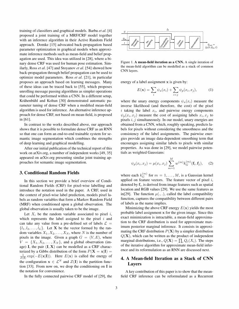
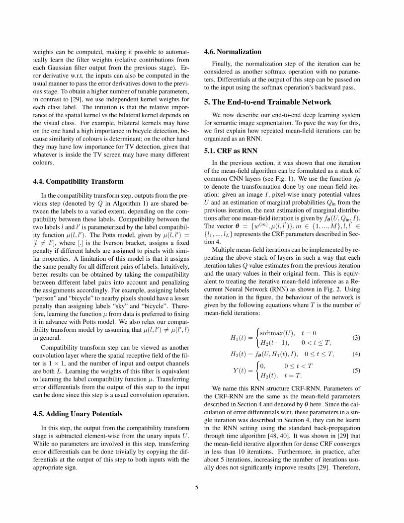
Figure 1. A mean-field iteration as a CNN. A single iteration ofthe mean-field algorithm can be modelled as a stack of commonCNN layers.

energy of a label assignment x is given by:

E(x) =∑i

ψu(xi) +∑i<j

ψp(xi, xj), (1)

where the unary energy components ψu(xi) measure theinverse likelihood (and therefore, the cost) of the pixeli taking the label xi, and pairwise energy componentsψp(xi, xj) measure the cost of assigning labels xi, xj topixels i, j simultaneously. In our model, unary energies areobtained from a CNN, which, roughly speaking, predicts la-bels for pixels without considering the smoothness and theconsistency of the label assignments. The pairwise ener-gies provide an image data-dependent smoothing term thatencourages assigning similar labels to pixels with similarproperties. As was done in [29], we model pairwise poten-tials as weighted Gaussians:

ψp(xi, xj) = µ(xi, xj)

M∑m=1

w(m)k(m)G (fi, fj), (2)

where each k(m)G for m = 1, . . . ,M , is a Gaussian kernel

applied on feature vectors. The feature vector of pixel i,denoted by fi, is derived from image features such as spatiallocation and RGB values [29]. We use the same features asin[29]. The function µ(., .), called the label compatibilityfunction, captures the compatibility between different pairsof labels as the name implies.

Minimizing the above CRF energy E(x) yields the mostprobable label assignment x for the given image. Since thisexact minimization is intractable, a mean-field approxima-tion to the CRF distribution is used for approximate max-imum posterior marginal inference. It consists in approxi-mating the CRF distribution P (X) by a simpler distributionQ(X), which can be written as the product of independentmarginal distributions, i.e., Q(X) =

∏iQi(Xi). The steps

of the iterative algorithm for approximate mean-field infer-ence and its reformulation as an RNN are discussed next.

4. A Mean-field Iteration as a Stack of CNNLayers

A key contribution of this paper is to show that the mean-field CRF inference can be reformulated as a Recurrent

3

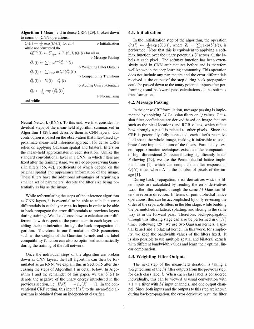
Algorithm 1 Mean-field in dense CRFs [29], broken downto common CNN operations.Qi(l)← 1

Ziexp (Ui(l)) for all i . Initialization

while not converged doQ

(m)i (l)←

∑j 6=i k

(m)(fi, fj)Qj(l) for all m. Message Passing

Qi(l)←∑

m w(m)Q(m)i (l)

. Weighting Filter OutputsQi(l)←

∑l′∈L µ(l, l′)Qi(l

′). Compatibility Transform

Qi(l)← Ui(l)− Qi(l). Adding Unary Potentials

Qi ← 1Zi

exp(Qi(l)

). Normalizing

end while

Neural Network (RNN). To this end, we first consider in-dividual steps of the mean-field algorithm summarized inAlgorithm 1 [29], and describe them as CNN layers. Ourcontribution is based on the observation that filter-based ap-proximate mean-field inference approach for dense CRFsrelies on applying Gaussian spatial and bilateral filters onthe mean-field approximates in each iteration. Unlike thestandard convolutional layer in a CNN, in which filters arefixed after the training stage, we use edge-preserving Gaus-sian filters [56, 42], coefficients of which depend on theoriginal spatial and appearance information of the image.These filters have the additional advantages of requiring asmaller set of parameters, despite the filter size being po-tentially as big as the image.

While reformulating the steps of the inference algorithmas CNN layers, it is essential to be able to calculate errordifferentials in each layer w.r.t. its inputs in order to be ableto back-propagate the error differentials to previous layersduring training. We also discuss how to calculate error dif-ferentials with respect to the parameters in each layer, en-abling their optimization through the back-propagation al-gorithm. Therefore, in our formulation, CRF parameterssuch as the weights of the Gaussian kernels and the labelcompatibility function can also be optimized automaticallyduring the training of the full network.

Once the individual steps of the algorithm are brokendown as CNN layers, the full algorithm can then be for-mulated as an RNN. We explain this in Section 5 after dis-cussing the steps of Algorithm 1 in detail below. In Algo-rithm 1 and the remainder of this paper, we use Ui(l) todenote the negative of the unary energy introduced in theprevious section, i.e., Ui(l) = −ψu(Xi = l). In the con-ventional CRF setting, this input Ui(l) to the mean-field al-gorithm is obtained from an independent classifier.

4.1. Initialization

In the initialization step of the algorithm, the operationQi(l) ← 1

Ziexp (Ui(l)), where Zi =

∑l exp(Ui(l)), is

performed. Note that this is equivalent to applying a soft-max function over the unary potentials U across all the la-bels at each pixel. The softmax function has been exten-sively used in CNN architectures before and is thereforewell known in the deep learning community. This operationdoes not include any parameters and the error differentialsreceived at the output of the step during back-propagationcould be passed down to the unary potential inputs after per-forming usual backward pass calculations of the softmaxtransformation.

4.2. Message Passing

In the dense CRF formulation, message passing is imple-mented by applying M Gaussian filters on Q values. Gaus-sian filter coefficients are derived based on image featuressuch as the pixel locations and RGB values, which reflecthow strongly a pixel is related to other pixels. Since theCRF is potentially fully connected, each filter’s receptivefield spans the whole image, making it infeasible to use abrute-force implementation of the filters. Fortunately, sev-eral approximation techniques exist to make computationof high dimensional Gaussian filtering significantly faster.Following [29], we use the Permutohedral lattice imple-mentation [1], which can compute the filter response inO(N) time, where N is the number of pixels of the im-age [1].

During back-propagation, error derivatives w.r.t. the fil-ter inputs are calculated by sending the error derivativesw.r.t. the filter outputs through the same M Gaussian fil-ters in reverse direction. In terms of permutohedral latticeoperations, this can be accomplished by only reversing theorder of the separable filters in the blur stage, while buildingthe permutohedral lattice, splatting, and slicing in the sameway as in the forward pass. Therefore, back-propagationthrough this filtering stage can also be performed in O(N)time. Following [29], we use two Gaussian kernels, a spa-tial kernel and a bilateral kernel. In this work, for simplic-ity, we keep the bandwidth values of the filters fixed. Itis also possible to use multiple spatial and bilateral kernelswith different bandwidth values and learn their optimal lin-ear combination.

4.3. Weighting Filter Outputs

The next step of the mean-field iteration is taking aweighted sum of theM filter outputs from the previous step,for each class label l. When each class label is consideredindividually, this can be viewed as usual convolution witha 1 × 1 filter with M input channels, and one output chan-nel. Since both inputs and the outputs to this step are knownduring back-propagation, the error derivative w.r.t. the filter

4

weights can be computed, making it possible to automat-ically learn the filter weights (relative contributions fromeach Gaussian filter output from the previous stage). Er-ror derivative w.r.t. the inputs can also be computed in theusual manner to pass the error derivatives down to the previ-ous stage. To obtain a higher number of tunable parameters,in contrast to [29], we use independent kernel weights foreach class label. The intuition is that the relative impor-tance of the spatial kernel vs the bilateral kernel depends onthe visual class. For example, bilateral kernels may haveon the one hand a high importance in bicycle detection, be-cause similarity of colours is determinant; on the other handthey may have low importance for TV detection, given thatwhatever is inside the TV screen may have many differentcolours.

4.4. Compatibility Transform

In the compatibility transform step, outputs from the pre-vious step (denoted by Q in Algorithm 1) are shared be-tween the labels to a varied extent, depending on the com-patibility between these labels. Compatibility between thetwo labels l and l′ is parameterized by the label compatibil-ity function µ(l, l′). The Potts model, given by µ(l, l′) =[l 6= l′], where [.] is the Iverson bracket, assigns a fixedpenalty if different labels are assigned to pixels with simi-lar properties. A limitation of this model is that it assignsthe same penalty for all different pairs of labels. Intuitively,better results can be obtained by taking the compatibilitybetween different label pairs into account and penalizingthe assignments accordingly. For example, assigning labels“person” and “bicycle” to nearby pixels should have a lesserpenalty than assigning labels “sky” and “bicycle”. There-fore, learning the function µ from data is preferred to fixingit in advance with Potts model. We also relax our compat-ibility transform model by assuming that µ(l, l′) 6= µ(l′, l)in general.

Compatibility transform step can be viewed as anotherconvolution layer where the spatial receptive field of the fil-ter is 1 × 1, and the number of input and output channelsare both L. Learning the weights of this filter is equivalentto learning the label compatibility function µ. Transferringerror differentials from the output of this step to the inputcan be done since this step is a usual convolution operation.

4.5. Adding Unary Potentials

In this step, the output from the compatibility transformstage is subtracted element-wise from the unary inputs U .While no parameters are involved in this step, transferringerror differentials can be done trivially by copying the dif-ferentials at the output of this step to both inputs with theappropriate sign.

4.6. Normalization

Finally, the normalization step of the iteration can beconsidered as another softmax operation with no parame-ters. Differentials at the output of this step can be passed onto the input using the softmax operation’s backward pass.

5. The End-to-end Trainable NetworkWe now describe our end-to-end deep learning system

for semantic image segmentation. To pave the way for this,we first explain how repeated mean-field iterations can beorganized as an RNN.

5.1. CRF as RNN

In the previous section, it was shown that one iterationof the mean-field algorithm can be formulated as a stack ofcommon CNN layers (see Fig. 1). We use the function fθto denote the transformation done by one mean-field iter-ation: given an image I , pixel-wise unary potential valuesU and an estimation of marginal probabilities Qin from theprevious iteration, the next estimation of marginal distribu-tions after one mean-field iteration is given by fθ(U,Qin, I).The vector θ = {w(m), µ(l, l

′)},m ∈ {1, ...,M}, l, l′ ∈

{l1, ..., lL} represents the CRF parameters described in Sec-tion 4.

Multiple mean-field iterations can be implemented by re-peating the above stack of layers in such a way that eachiteration takesQ value estimates from the previous iterationand the unary values in their original form. This is equiv-alent to treating the iterative mean-field inference as a Re-current Neural Network (RNN) as shown in Fig. 2. Usingthe notation in the figure, the behaviour of the network isgiven by the following equations where T is the number ofmean-field iterations:

H1(t) =

{softmax(U), t = 0

H2(t− 1), 0 < t ≤ T,(3)

H2(t) = fθ(U,H1(t), I), 0 ≤ t ≤ T, (4)

Y (t) =

{0, 0 ≤ t < T

H2(t), t = T.(5)

We name this RNN structure CRF-RNN. Parameters ofthe CRF-RNN are the same as the mean-field parametersdescribed in Section 4 and denoted by θ here. Since the cal-culation of error differentials w.r.t. these parameters in a sin-gle iteration was described in Section 4, they can be learntin the RNN setting using the standard back-propagationthrough time algorithm [48, 40]. It was shown in [29] thatthe mean-field iterative algorithm for dense CRF convergesin less than 10 iterations. Furthermore, in practice, afterabout 5 iterations, increasing the number of iterations usu-ally does not significantly improve results [29]. Therefore,

5

MeanfieldIteration

H2 =fθ(U,H1, I)

I

U

SoftmaxNormalization

G1

G2

YH2

H1

1

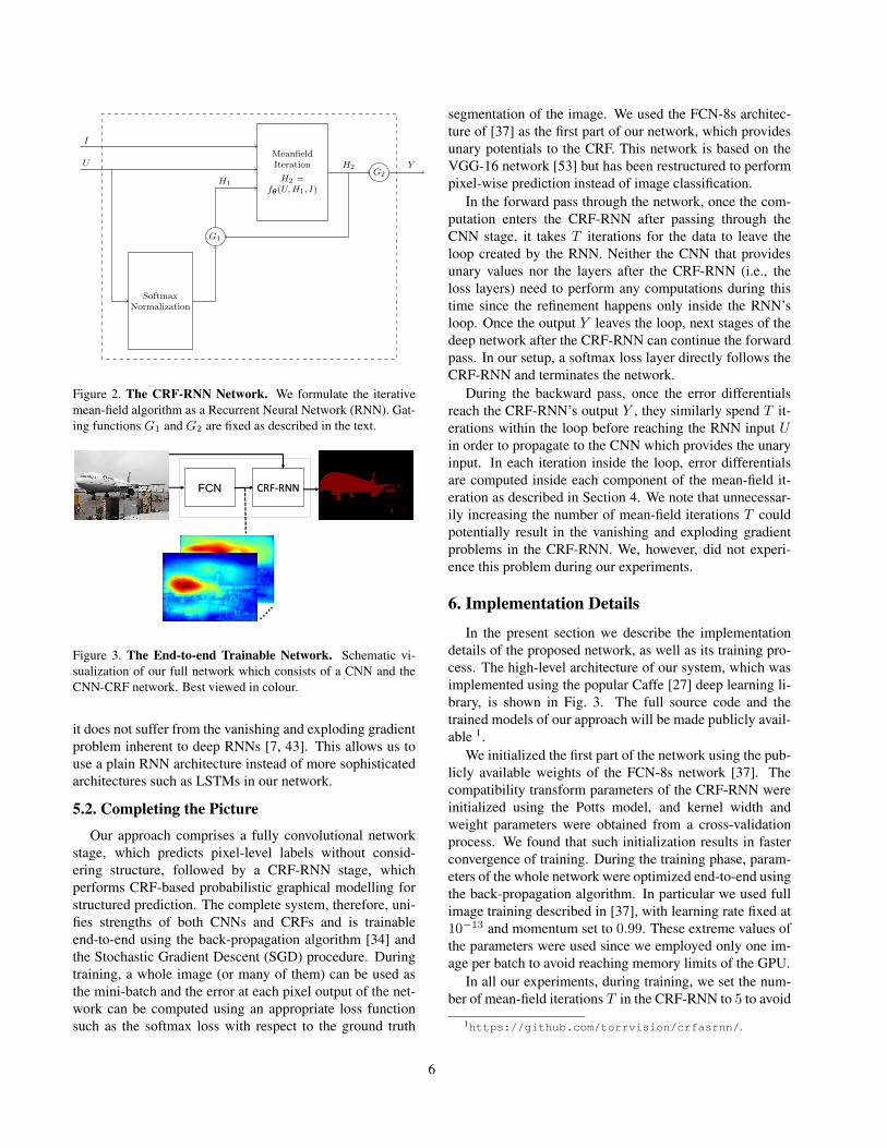
Figure 2. The CRF-RNN Network. We formulate the iterativemean-field algorithm as a Recurrent Neural Network (RNN). Gat-ing functions G1 and G2 are fixed as described in the text.

FCN CRF-RNN

Figure 3. The End-to-end Trainable Network. Schematic vi-sualization of our full network which consists of a CNN and theCNN-CRF network. Best viewed in colour.

it does not suffer from the vanishing and exploding gradientproblem inherent to deep RNNs [7, 43]. This allows us touse a plain RNN architecture instead of more sophisticatedarchitectures such as LSTMs in our network.

5.2. Completing the Picture

Our approach comprises a fully convolutional networkstage, which predicts pixel-level labels without consid-ering structure, followed by a CRF-RNN stage, whichperforms CRF-based probabilistic graphical modelling forstructured prediction. The complete system, therefore, uni-fies strengths of both CNNs and CRFs and is trainableend-to-end using the back-propagation algorithm [34] andthe Stochastic Gradient Descent (SGD) procedure. Duringtraining, a whole image (or many of them) can be used asthe mini-batch and the error at each pixel output of the net-work can be computed using an appropriate loss functionsuch as the softmax loss with respect to the ground truth

segmentation of the image. We used the FCN-8s architec-ture of [37] as the first part of our network, which providesunary potentials to the CRF. This network is based on theVGG-16 network [53] but has been restructured to performpixel-wise prediction instead of image classification.

In the forward pass through the network, once the com-putation enters the CRF-RNN after passing through theCNN stage, it takes T iterations for the data to leave theloop created by the RNN. Neither the CNN that providesunary values nor the layers after the CRF-RNN (i.e., theloss layers) need to perform any computations during thistime since the refinement happens only inside the RNN’sloop. Once the output Y leaves the loop, next stages of thedeep network after the CRF-RNN can continue the forwardpass. In our setup, a softmax loss layer directly follows theCRF-RNN and terminates the network.

During the backward pass, once the error differentialsreach the CRF-RNN’s output Y , they similarly spend T it-erations within the loop before reaching the RNN input Uin order to propagate to the CNN which provides the unaryinput. In each iteration inside the loop, error differentialsare computed inside each component of the mean-field it-eration as described in Section 4. We note that unnecessar-ily increasing the number of mean-field iterations T couldpotentially result in the vanishing and exploding gradientproblems in the CRF-RNN. We, however, did not experi-ence this problem during our experiments.

6. Implementation Details

In the present section we describe the implementationdetails of the proposed network, as well as its training pro-cess. The high-level architecture of our system, which wasimplemented using the popular Caffe [27] deep learning li-brary, is shown in Fig. 3. The full source code and thetrained models of our approach will be made publicly avail-able 1.

We initialized the first part of the network using the pub-licly available weights of the FCN-8s network [37]. Thecompatibility transform parameters of the CRF-RNN wereinitialized using the Potts model, and kernel width andweight parameters were obtained from a cross-validationprocess. We found that such initialization results in fasterconvergence of training. During the training phase, param-eters of the whole network were optimized end-to-end usingthe back-propagation algorithm. In particular we used fullimage training described in [37], with learning rate fixed at10−13 and momentum set to 0.99. These extreme values ofthe parameters were used since we employed only one im-age per batch to avoid reaching memory limits of the GPU.

In all our experiments, during training, we set the num-ber of mean-field iterations T in the CRF-RNN to 5 to avoid

1https://github.com/torrvision/crfasrnn/.

6

vanishing/exploding gradient problems and to reduce thetraining time. During the test time, iteration count was in-creased to 10. The effect of this parameter value on theaccuracy is discussed in section 7.1.

Loss function During the training of the models thatachieved the best results reported in this paper, we used thestandard softmax loss function, that is, the log-likelihooderror function described in [30]. The standard metric usedin the Pascal VOC challenge is the average intersection overunion (IU), which we also use here to report the results. Inour experiments we found that high values of IU on the val-idation set were associated to low values of the averagedsoftmax loss, to a large extent. We also tried the robust log-likelihood in [30] as a loss function for CRF-RNN training.However, this did not result in increased accuracy nor fasterconvergence.

Normalization techniques As described in Section 4,we use the exponential function followed by pixel-wise nor-malization across channels in several stages of the CRF-RNN. Since this operation has a tendency to result in smallgradients with respect to the input when the input value islarge, we conducted several experiments where we replacedthis by a rectifier linear unit (ReLU) operation followed bya normalization across the channels. Our hypothesis wasthat this approach may approximate the original operationadequately while speeding up the training due to improvedgradients. Furthermore, ReLU would induce sparsity on theprobability of labels assigned to pixels, implicitly pruninglow likelihood configurations, which could have a positiveeffect. However, this approach did not lead to better re-sults, obtaining 1% IU lower than the original setting per-formance.

7. ExperimentsWe present experimental results with the proposed CRF-

RNN framework. We use these datasets: the Pascal VOC2012 dataset, and the Pascal Context dataset. We use thePascal VOC 2012 dataset as it has become the golden stan-dard to comprehensively evaluate any new semantic seg-mentation approach in comparison to existing methods. Wealso use the Pascal Context dataset to assess how well ourapproach performs on a dataset with different characteris-tics.

Pascal VOC Datasets

In order to evaluate our approach with existing methods un-der the same circumstances, we conducted two main exper-iments with the Pascal VOC 2012 dataset, followed by aqualitative experiment.

In the first experiment, following [37, 38, 41], we useda training set consisted of VOC 2012 training data (1464images), and training and validation data of [23], which

Input Image Ground TruthCRF-RNNDeepLabFCN-8s

B-ground Aero plane Bicycle Bird Boat Bottle Bus

Car Cat Chair Cow Dining-Table Dog Horse

Motorbike Person Potted-Plant Sheep Sofa Train TV/Monitor

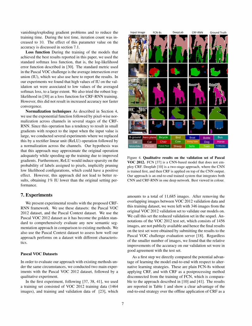
Figure 4. Qualitative results on the validation set of PascalVOC 2012. FCN [37] is a CNN-based model that does not em-ploy CRF. Deeplab [10] is a two-stage approach, where the CNNis trained first, and then CRF is applied on top of the CNN output.Our approach is an end-to-end trained system that integrates bothCNN and CRF-RNN in one deep network. Best viewed in colour.

amounts to a total of 11,685 images. After removing theoverlapping images between VOC 2012 validation data andthis training dataset, we were left with 346 images from theoriginal VOC 2012 validation set to validate our models on.We call this set the reduced validation set in the sequel. An-notations of the VOC 2012 test set, which consists of 1456images, are not publicly available and hence the final resultson the test set were obtained by submitting the results to thePascal VOC challenge evaluation server [18]. Regardlessof the smaller number of images, we found that the relativeimprovements of the accuracy on our validation set were ingood agreement with the test set.

As a first step we directly compared the potential advan-tage of learning the model end-to-end with respect to alter-native learning strategies. These are plain FCN-8s withoutapplying CRF, and with CRF as a postprocessing methoddisconnected from the training of FCN, which is compara-ble to the approach described in [10] and [41]. The resultsare reported in Table 1 and show a clear advantage of theend-to-end strategy over the offline application of CRF as a

7

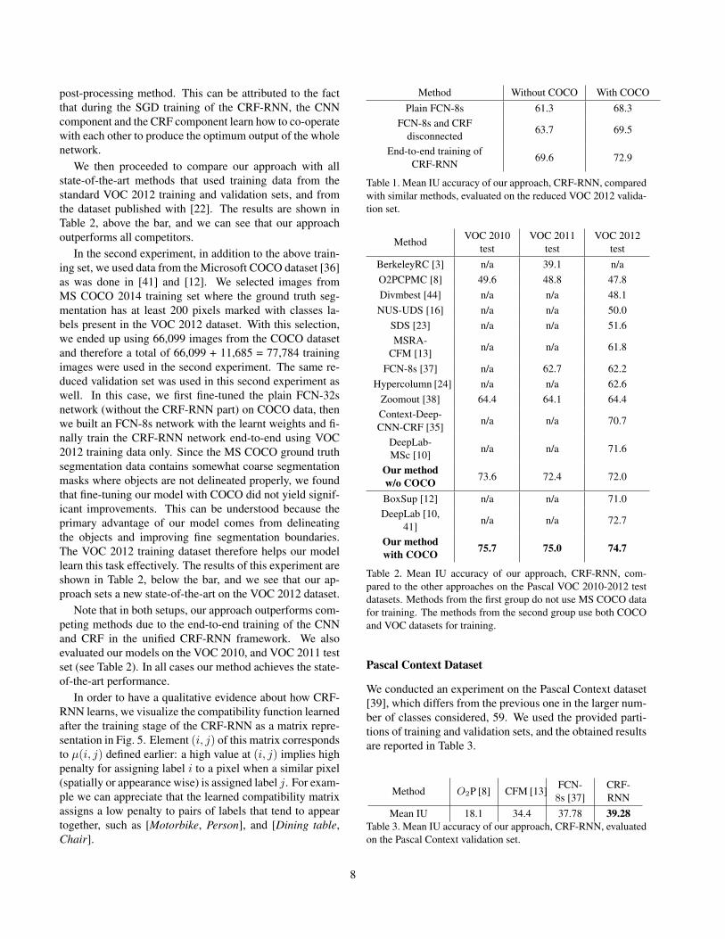
post-processing method. This can be attributed to the factthat during the SGD training of the CRF-RNN, the CNNcomponent and the CRF component learn how to co-operatewith each other to produce the optimum output of the wholenetwork.

We then proceeded to compare our approach with allstate-of-the-art methods that used training data from thestandard VOC 2012 training and validation sets, and fromthe dataset published with [22]. The results are shown inTable 2, above the bar, and we can see that our approachoutperforms all competitors.

In the second experiment, in addition to the above train-ing set, we used data from the Microsoft COCO dataset [36]as was done in [41] and [12]. We selected images fromMS COCO 2014 training set where the ground truth seg-mentation has at least 200 pixels marked with classes la-bels present in the VOC 2012 dataset. With this selection,we ended up using 66,099 images from the COCO datasetand therefore a total of 66,099 + 11,685 = 77,784 trainingimages were used in the second experiment. The same re-duced validation set was used in this second experiment aswell. In this case, we first fine-tuned the plain FCN-32snetwork (without the CRF-RNN part) on COCO data, thenwe built an FCN-8s network with the learnt weights and fi-nally train the CRF-RNN network end-to-end using VOC2012 training data only. Since the MS COCO ground truthsegmentation data contains somewhat coarse segmentationmasks where objects are not delineated properly, we foundthat fine-tuning our model with COCO did not yield signif-icant improvements. This can be understood because theprimary advantage of our model comes from delineatingthe objects and improving fine segmentation boundaries.The VOC 2012 training dataset therefore helps our modellearn this task effectively. The results of this experiment areshown in Table 2, below the bar, and we see that our ap-proach sets a new state-of-the-art on the VOC 2012 dataset.

Note that in both setups, our approach outperforms com-peting methods due to the end-to-end training of the CNNand CRF in the unified CRF-RNN framework. We alsoevaluated our models on the VOC 2010, and VOC 2011 testset (see Table 2). In all cases our method achieves the state-of-the-art performance.

In order to have a qualitative evidence about how CRF-RNN learns, we visualize the compatibility function learnedafter the training stage of the CRF-RNN as a matrix repre-sentation in Fig. 5. Element (i, j) of this matrix correspondsto µ(i, j) defined earlier: a high value at (i, j) implies highpenalty for assigning label i to a pixel when a similar pixel(spatially or appearance wise) is assigned label j. For exam-ple we can appreciate that the learned compatibility matrixassigns a low penalty to pairs of labels that tend to appeartogether, such as [Motorbike, Person], and [Dining table,Chair].

Method Without COCO With COCOPlain FCN-8s 61.3 68.3

FCN-8s and CRFdisconnected

63.7 69.5

End-to-end training ofCRF-RNN

69.6 72.9

Table 1. Mean IU accuracy of our approach, CRF-RNN, comparedwith similar methods, evaluated on the reduced VOC 2012 valida-tion set.

MethodVOC 2010

testVOC 2011

testVOC 2012

testBerkeleyRC [3] n/a 39.1 n/aO2PCPMC [8] 49.6 48.8 47.8Divmbest [44] n/a n/a 48.1NUS-UDS [16] n/a n/a 50.0

SDS [23] n/a n/a 51.6MSRA-

CFM [13]n/a n/a 61.8

FCN-8s [37] n/a 62.7 62.2Hypercolumn [24] n/a n/a 62.6

Zoomout [38] 64.4 64.1 64.4Context-Deep-CNN-CRF [35]

n/a n/a 70.7

DeepLab-MSc [10]

n/a n/a 71.6

Our methodw/o COCO 73.6 72.4 72.0

BoxSup [12] n/a n/a 71.0DeepLab [10,

41]n/a n/a 72.7

Our methodwith COCO 75.7 75.0 74.7

Table 2. Mean IU accuracy of our approach, CRF-RNN, com-pared to the other approaches on the Pascal VOC 2010-2012 testdatasets. Methods from the first group do not use MS COCO datafor training. The methods from the second group use both COCOand VOC datasets for training.

Pascal Context Dataset

We conducted an experiment on the Pascal Context dataset[39], which differs from the previous one in the larger num-ber of classes considered, 59. We used the provided parti-tions of training and validation sets, and the obtained resultsare reported in Table 3.

Method O2P [8] CFM [13]FCN-8s [37]

CRF-RNN

Mean IU 18.1 34.4 37.78 39.28Table 3. Mean IU accuracy of our approach, CRF-RNN, evaluatedon the Pascal Context validation set.

8

-0.9

-0.8

-0.7

-0.6

-0.5

-0.4

-0.3

-0.2

-0.1

00.0

-1.0

-0.5

B-Ground

Aeroplane

Bicycle

Bird

Boat

Bus

Car

Cat

Chair

CowDining-Table

Dog

Horse

Motorbike

Person

PottlePlant

Sheep

Sofa

Train

TV/Monitor

Bottle

B-G

rou

nd

Aero

pla

ne

Bic

ycle

Bir

d

Bo

at

Bu

s

Car

Cat

Ch

air

Co

wD

inin

g-T

ab

le

Do

g

Ho

rse

Mo

torb

ike

Pers

on

Po

ttle

Pla

nt

Sh

eep

So

fa

Tra

in

TV

/Mo

nit

or

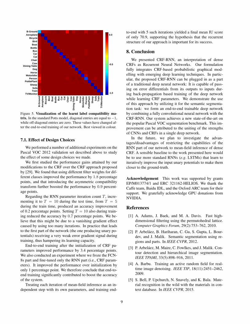
Bo

ttle

Figure 5. Visualization of the learnt label compatibility ma-trix. In the standard Potts model, diagonal entries are equal to−1,while off-diagonal entries are zero. These values have changed af-ter the end-to-end training of our network. Best viewed in colour.

7.1. Effect of Design Choices

We performed a number of additional experiments on thePascal VOC 2012 validation set described above to studythe effect of some design choices we made.

We first studied the performance gains attained by ourmodifications to the CRF over the CRF approach proposedby [29]. We found that using different filter weights for dif-ferent classes improved the performance by 1.8 percentagepoints, and that introducing the asymmetric compatibilitytransform further boosted the performance by 0.9 percent-age points.

Regarding the RNN parameter iteration count T , incre-menting it to T = 10 during the test time, from T = 5during the train time, produced an accuracy improvementof 0.2 percentage points. Setting T = 10 also during train-ing reduced the accuracy by 0.7 percentage points. We be-lieve that this might be due to a vanishing gradient effectcaused by using too many iterations. In practice that leadsto the first part of the network (the one producing unary po-tentials) receiving a very weak error gradient signal duringtraining, thus hampering its learning capacity.

End-to-end training after the initialization of CRF pa-rameters improved performance by 3.4 percentage points.We also conducted an experiment where we froze the FCN-8s part and fine-tuned only the RNN part (i.e., CRF param-eters). It improved the performance over initialization byonly 1 percentage point. We therefore conclude that end-to-end training significantly contributed to boost the accuracyof the system.

Treating each iteration of mean-field inference as an in-dependent step with its own parameters, and training end-

to-end with 5 such iterations yielded a final mean IU scoreof only 70.9, supporting the hypothesis that the recurrentstructure of our approach is important for its success.

8. ConclusionWe presented CRF-RNN, an interpretation of dense

CRFs as Recurrent Neural Networks. Our formulationfully integrates CRF-based probabilistic graphical mod-elling with emerging deep learning techniques. In partic-ular, the proposed CRF-RNN can be plugged in as a partof a traditional deep neural network: It is capable of pass-ing on error differentials from its outputs to inputs dur-ing back-propagation based training of the deep networkwhile learning CRF parameters. We demonstrate the useof this approach by utilizing it for the semantic segmenta-tion task: we form an end-to-end trainable deep networkby combining a fully convolutional neural network with theCRF-RNN. Our system achieves a new state-of-the-art onthe popular Pascal VOC segmentation benchmark. This im-provement can be attributed to the uniting of the strengthsof CNNs and CRFs in a single deep network.

In the future, we plan to investigate the advan-tages/disadvantages of restricting the capabilities of theRNN part of our network to mean-field inference of denseCRF. A sensible baseline to the work presented here wouldbe to use more standard RNNs (e.g. LSTMs) that learn toiteratively improve the input unary potentials to make themcloser to the ground-truth.

Acknowledgement This work was supported by grantsEP/M013774/1 and ERC 321162-HELIOS. We thank theCaffe team, Baidu IDL, and the Oxford ARC team for theirsupport. We gratefully acknowledge GPU donations fromNVIDIA.

References[1] A. Adams, J. Baek, and M. A. Davis. Fast high-

dimensional filtering using the permutohedral lattice.Computer Graphics Forum, 29(2):753–762, 2010.

[2] P. Arbelaez, B. Hariharan, C. Gu, S. Gupta, L. Bour-dev, and J. Malik. Semantic segmentation using re-gions and parts. In IEEE CVPR, 2012.

[3] P. Arbelaez, M. Maire, C. Fowlkes, and J. Malik. Con-tour detection and hierarchical image segmentation.IEEE TPAMI, 33(5):898–916, 2011.

[4] A. Barbu. Training an active random field for real-time image denoising. IEEE TIP, 18(11):2451–2462,2009.

[5] S. Bell, P. Upchurch, N. Snavely, and K. Bala. Mate-rial recognition in the wild with the materials in con-text database. In IEEE CVPR, 2015.

9

[6] Y. Bengio, Y. LeCun, and D. Henderson. Globallytrained handwritten word recognizer using spatial rep-resentation, convolutional neural networks, and hid-den markov models. In NIPS, pages 937–937, 1994.

[7] Y. Bengio, P. Simard, and P. Frasconi. Learning long-term dependencies with gradient descent is difficult.IEEE Transactions on Neural Networks, 1994.

[8] J. Carreira, R. Caseiro, J. Batista, and C. Sminchis-escu. Free-form region description with second-orderpooling. IEEE TPAMI, 2014.

[9] K. Chatfield, K. Simonyan, A. Vedaldi, and A. Zisser-man. Return of the devil in the details: Delving deepinto convolutional nets. In BMVC, 2014.

[10] L.-C. Chen, G. Papandreou, I. Kokkinos, K. Murphy,and A. L. Yuille. Semantic image segmentation withdeep convolutional nets and fully connected crfs. InICLR, 2015.

[11] L.-C. Chen, A. G. Schwing, A. L. Yuille, and R. Ur-tasun. Learning deep structured models. In ICLRW,2015.

[12] J. Dai, K. He, and J. Sun. Boxsup: Exploiting bound-ing boxes to supervise convolutional networks for se-mantic segmentation. In arXiv:1503.01640, 2015.

[13] J. Dai, K. He, and J. Sun. Convolutional feature mask-ing for joint object and stuff segmentation. In IEEECVPR, 2015.

[14] T.-M.-T. Do and T. Artieres. Neural conditional ran-dom fields. In NIPS, 2010.

[15] J. Domke. Learning graphical model parameterswith approximate marginal inference. IEEE TPAMI,35(10):2454–2467, 2013.

[16] J. Dong, Q. Chen, S. Yan, and A. Yuille. Towardsunified object detection and semantic segmentation. InECCV, 2014.

[17] D. Eigen, C. Puhrsch, and R. Fergus. Depth map pre-diction from a single image using a multi-scale deepnetwork. In NIPS, 2014.

[18] M. Everingham, S. M. A. Eslami, L. Van Gool, C. K. I.Williams, J. Winn, and A. Zisserman. The pascal vi-sual object classes challenge: A retrospective. IJCV,111(1):98–136, 2015.

[19] C. Farabet, C. Couprie, L. Najman, and Y. Le-Cun. Learning hierarchical features for scene labeling.IEEE TPAMI, 2013.

[20] R. Girshick, J. Donahue, T. Darrell, and J. Malik. Richfeature hierarchies for accurate object detection andsemantic segmentation. In IEEE CVPR, 2014.

[21] R. Girshick, F. Iandola, T. Darrell, and J. Malik. De-formable part models are convolutional neural net-works. In CVPR, 2015.

[22] B. Hariharan, P. Arbelaez, L. D. Bourdev, S. Maji, andJ. Malik. Semantic contours from inverse detectors. InIEEE ICCV, 2011.

[23] B. Hariharan, P. Arbelaez, R. Girshick, and J. Malik.Simultaneous detection and segmentation. In ECCV,2014.

[24] B. Hariharan, P. Arbelaez, R. Girshick, and J. Ma-lik. Hypercolumns for object segmentation and fine-grained localization. In IEEE CVPR, 2015.

[25] M. Jaderberg, K. Simonyan, A. Vedaldi, and A. Zis-serman. Deep structured output learning for uncon-strained text recognition. In ICLR, 2015.

[26] V. Jain, J. F. Murray, F. Roth, S. C. Turaga, V. P.Zhigulin, K. L. Briggman, M. Helmstaedter, W. Denk,and H. S. Seung. Supervised learning of imagerestoration with convolutional networks. In IEEEICCV, 2007.

[27] Y. Jia, E. Shelhamer, J. Donahue, S. Karayev, J. Long,R. Girshick, S. Guadarrama, and T. Darrell. Caffe:Convolutional architecture for fast feature embedding.In ACM Multimedia, pages 675–678, 2014.

[28] M. Kiefel and P. V. Gehler. Human pose estmationwith fields of parts. In ECCV, 2014.

[29] P. Krahenbuhl and V. Koltun. Efficient inference infully connected crfs with gaussian edge potentials. InNIPS, 2011.

[30] P. Krahenbuhl and V. Koltun. Parameter learningand convergent inference for dense random fields. InICML, 2013.

[31] A. Krizhevsky, I. Sutskever, and G. E. Hinton. Im-agenet classification with deep convolutional neuralnetworks. In NIPS, 2012.

[32] L. Ladicky, C. Russell, P. Kohli, and P. H. Torr. As-sociative hierarchical crfs for object class image seg-mentation. In IEEE ICCV, 2009.

[33] J. D. Lafferty, A. McCallum, and F. C. N. Pereira.Conditional random fields: Probabilistic models forsegmenting and labeling sequence data. In ICML,2001.

[34] Y. LeCun, L. Bottou, Y. Bengio, and P. Haffner.Gradient-based learning applied to document recog-nition. Proceedings of the IEEE, 86(11):2278–2324,1998.

[35] G. Lin, C. Shen, I. Reid, and A. van dan Hengel. Effi-cient piecewise training of deep structured models forsemantic segmentation. In arXiv:1504.01013, 2015.

[36] T.-Y. Lin, M. Maire, S. Belongie, L. Bourdev, R. Gir-shick, J. Hays, P. Perona, D. Ramanan, C. L. Zitnick,and P. Dollar. Microsoft coco: Common objects incontext. In arXiv:1405.0312, 2014.

10

[37] J. Long, E. Shelhamer, and T. Darrell. Fully convolu-tional networks for semantic segmentation. In IEEECVPR, 2015.

[38] M. Mostajabi, P. Yadollahpour, and G. Shakhnarovich.Feedforward semantic segmentation with zoom-outfeatures. In IEEE CVPR, 2015.

[39] R. Mottaghi, X. Chen, X. Liu, N.-G. Cho, S.-W. Lee,S. Fidler, R. Urtasun, and A. Yuille. The role of con-text for object detection and semantic segmentation inthe wild. In IEEE CVPR, 2014.

[40] M. C. Mozer. Backpropagation. In Y. Chauvin andD. E. Rumelhart, editors, Backpropagation, chapterA Focused Backpropagation Algorithm for TemporalPattern Recognition, pages 137–169. L. Erlbaum As-sociates Inc., 1995.

[41] G. Papandreou, L.-C. Chen, K. Murphy, and A. L.Yuille. Weakly- and semi-supervised learning ofa dcnn for semantic image segmentation. InarXiv:1502.02734, 2015.

[42] S. Paris and F. Durand. A fast approximation of the bi-lateral filter using a signal processing approach. IJCV,81(1):24–52, 2013.

[43] R. Pascanu, C. Gulcehre, K. Cho, and Y. Bengio. Onthe difficulty of training recurrent neural networks. InICML, 2013.

[44] G. S. Payman Yadollahpour, Dhruv Batra. Discrimi-native re-ranking of diverse segmentations. In IEEECVPR, 2013.

[45] J. Peng, L. Bo, and J. Xu. Conditional neural fields.In NIPS, 2009.

[46] P. H. O. Pinheiro and R. Collobert. Recurrent convo-lutional neural networks for scene labeling. In ICML,2014.

[47] S. Ross, D. Munoz, M. Hebert, and J. A. Bag-nell. Learning message-passing inference machinesfor structured prediction. In IEEE CVPR, 2011.

[48] D. E. Rumelhart, G. E. Hinton, and R. J. Williams.Parallel distributed processing: explorations in themicrostructure of cognition. In J. A. Anderson andE. Rosenfeld, editors, Parallel distributed processing:explorations in the microstructure of cognition, chap-ter Learning Internal Representations by Error Propa-gation, pages 318–362. MIT Press, 1986.

[49] A. G. Schwing and R. Urtasun. Fully connected deepstructured networks. In arXiv:1503.02351, 2015.

[50] J. Shotton, A. Fitzgibbon, M. Cook, T. Sharp,M. Finocchio, R. Moore, A. Kipman, and A. Blake.Real-time human pose recognition in parts from sin-gle depth images. In IEEE CVPR, 2011.

[51] J. Shotton, M. Johnson, and R. Cipolla. Semantic tex-ton forests for image categorization and segmentation.In IEEE CVPR, 2008.

[52] J. Shotton, J. Winn, C. Rother, and A. Criminisi. Tex-tonboost for image understanding: Multi-class objectrecognition and segmentation by jointly modeling tex-ture, layout, and context. IJCV, 81(1):2–23, 2009.

[53] K. Simonyan and A. Zisserman. Very deep convolu-tional networks for large-scale image recognition. InarXiv:1409.1556, 2014.

[54] V. Stoyanov, A. Ropson, and J. Eisner. Empirical riskminimization of graphical model parameters given ap-proximate inference, decoding, and model structure.In AISTATS, 2011.

[55] S. C. Tatikonda and M. I. Jordan. Loopy belief prop-agation and gibbs measures. In Proceedings of theEighteenth Conference on Uncertainty in Artificial In-telligence, 2002.

[56] C. Tomasi and R. Manduchi. Bilateral filtering forgray and color images. In IEEE CVPR, 1998.

[57] J. J. Tompson, A. Jain, Y. LeCun, and C. Bregler. Jointtraining of a convolutional network and a graphicalmodel for human pose estimation. In NIPS, 2014.

[58] Z. Tu. Auto-context and its application to high-levelvision tasks. In IEEE CVPR, 2008.

[59] Z. Tu, X. Chen, A. L. Yuille, and S.-C. Zhu. Imageparsing: Unifying segmentation, detection, and recog-nition. IJCV, 63(2):113–140, 2005.

[60] K. Yao, B. Peng, G. Zweig, D. Yu, X. Li, and F. Gao.Recurrent conditional random field for language un-derstanding. In ICASSP, 2014.

[61] Y. Zhang and T. Chen. Efficient inference for fully-connected crfs with stationarity. In CVPR, 2012.

11

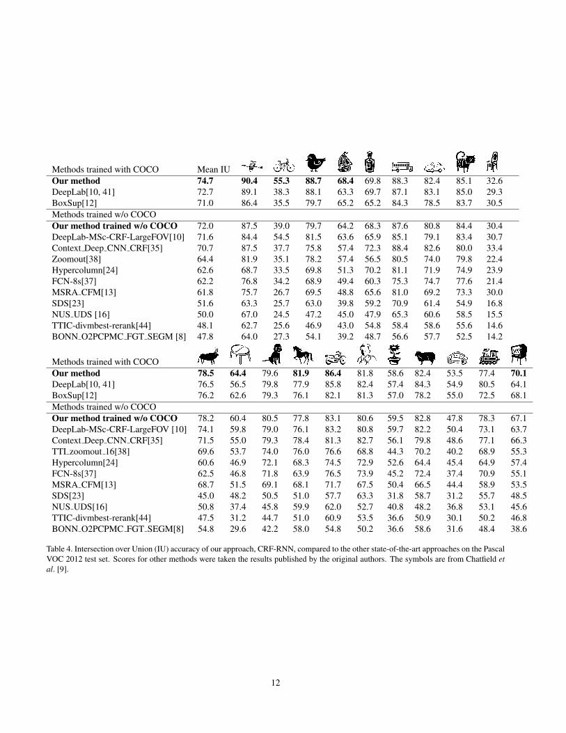
Methods trained with COCO Mean IUOur method 74.7 90.4 55.3 88.7 68.4 69.8 88.3 82.4 85.1 32.6DeepLab[10, 41] 72.7 89.1 38.3 88.1 63.3 69.7 87.1 83.1 85.0 29.3BoxSup[12] 71.0 86.4 35.5 79.7 65.2 65.2 84.3 78.5 83.7 30.5Methods trained w/o COCOOur method trained w/o COCO 72.0 87.5 39.0 79.7 64.2 68.3 87.6 80.8 84.4 30.4DeepLab-MSc-CRF-LargeFOV[10] 71.6 84.4 54.5 81.5 63.6 65.9 85.1 79.1 83.4 30.7Context Deep CNN CRF[35] 70.7 87.5 37.7 75.8 57.4 72.3 88.4 82.6 80.0 33.4Zoomout[38] 64.4 81.9 35.1 78.2 57.4 56.5 80.5 74.0 79.8 22.4Hypercolumn[24] 62.6 68.7 33.5 69.8 51.3 70.2 81.1 71.9 74.9 23.9FCN-8s[37] 62.2 76.8 34.2 68.9 49.4 60.3 75.3 74.7 77.6 21.4MSRA CFM[13] 61.8 75.7 26.7 69.5 48.8 65.6 81.0 69.2 73.3 30.0SDS[23] 51.6 63.3 25.7 63.0 39.8 59.2 70.9 61.4 54.9 16.8NUS UDS [16] 50.0 67.0 24.5 47.2 45.0 47.9 65.3 60.6 58.5 15.5TTIC-divmbest-rerank[44] 48.1 62.7 25.6 46.9 43.0 54.8 58.4 58.6 55.6 14.6BONN O2PCPMC FGT SEGM [8] 47.8 64.0 27.3 54.1 39.2 48.7 56.6 57.7 52.5 14.2

Methods trained with COCOOur method 78.5 64.4 79.6 81.9 86.4 81.8 58.6 82.4 53.5 77.4 70.1DeepLab[10, 41] 76.5 56.5 79.8 77.9 85.8 82.4 57.4 84.3 54.9 80.5 64.1BoxSup[12] 76.2 62.6 79.3 76.1 82.1 81.3 57.0 78.2 55.0 72.5 68.1Methods trained w/o COCOOur method trained w/o COCO 78.2 60.4 80.5 77.8 83.1 80.6 59.5 82.8 47.8 78.3 67.1DeepLab-MSc-CRF-LargeFOV [10] 74.1 59.8 79.0 76.1 83.2 80.8 59.7 82.2 50.4 73.1 63.7Context Deep CNN CRF[35] 71.5 55.0 79.3 78.4 81.3 82.7 56.1 79.8 48.6 77.1 66.3TTI zoomout 16[38] 69.6 53.7 74.0 76.0 76.6 68.8 44.3 70.2 40.2 68.9 55.3Hypercolumn[24] 60.6 46.9 72.1 68.3 74.5 72.9 52.6 64.4 45.4 64.9 57.4FCN-8s[37] 62.5 46.8 71.8 63.9 76.5 73.9 45.2 72.4 37.4 70.9 55.1MSRA CFM[13] 68.7 51.5 69.1 68.1 71.7 67.5 50.4 66.5 44.4 58.9 53.5SDS[23] 45.0 48.2 50.5 51.0 57.7 63.3 31.8 58.7 31.2 55.7 48.5NUS UDS[16] 50.8 37.4 45.8 59.9 62.0 52.7 40.8 48.2 36.8 53.1 45.6TTIC-divmbest-rerank[44] 47.5 31.2 44.7 51.0 60.9 53.5 36.6 50.9 30.1 50.2 46.8BONN O2PCPMC FGT SEGM[8] 54.8 29.6 42.2 58.0 54.8 50.2 36.6 58.6 31.6 48.4 38.6

Table 4. Intersection over Union (IU) accuracy of our approach, CRF-RNN, compared to the other state-of-the-art approaches on the PascalVOC 2012 test set. Scores for other methods were taken the results published by the original authors. The symbols are from Chatfield etal. [9].

12

Input Image CRF-RNN Ground Truth

B-g

rou

nd

Ae

ro p

lan

eB

icycle

Bird

Bo

at

Bo

ttle

Bu

s

Ca

rC

at

Ch

air

Co

wD

inin

g-T

able

Do

gH

ors

e

Moto

rbik

eP

ers

on

Pott

ed-P

lant

Sh

ee

pS

ofa

Tra

inT

V/M

onitor

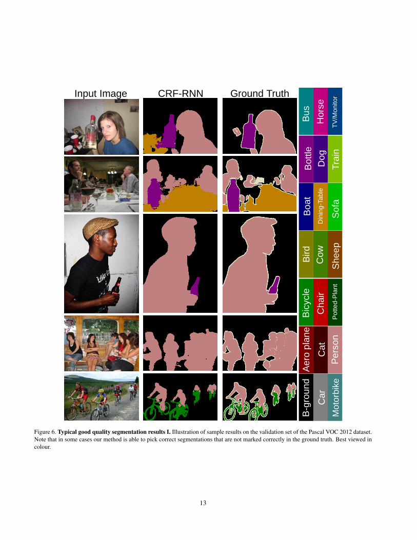
Figure 6. Typical good quality segmentation results I. Illustration of sample results on the validation set of the Pascal VOC 2012 dataset.Note that in some cases our method is able to pick correct segmentations that are not marked correctly in the ground truth. Best viewed incolour.

13

Input Image CRF-RNN Ground Truth

B-g

rou

nd

Ae

ro p

lan

eB

icycle

Bird

Bo

at

Bo

ttle

Bu

s

Ca

rC

at

Ch

air

Co

wD

inin

g-T

able

Do

gH

ors

e

Moto

rbik

eP

ers

on

Pott

ed-P

lant

Sh

ee

pS

ofa

Tra

inT

V/M

onitor

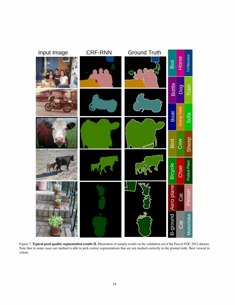
Figure 7. Typical good quality segmentation results II. Illustration of sample results on the validation set of the Pascal VOC 2012 dataset.Note that in some cases our method is able to pick correct segmentations that are not marked correctly in the ground truth. Best viewed incolour.

14

Input Image CRF-RNN Ground Truth

B-g

rou

nd

Ae

ro p

lan

eB

icycle

Bird

Bo

at

Bo

ttle

Bu

s

Ca

rC

at

Ch

air

Co

wD

inin

g-T

able

Do

gH

ors

e

Moto

rbik

eP

ers

on

Pott

ed-P

lant

Sh

ee

pS

ofa

Tra

inT

V/M

onitor

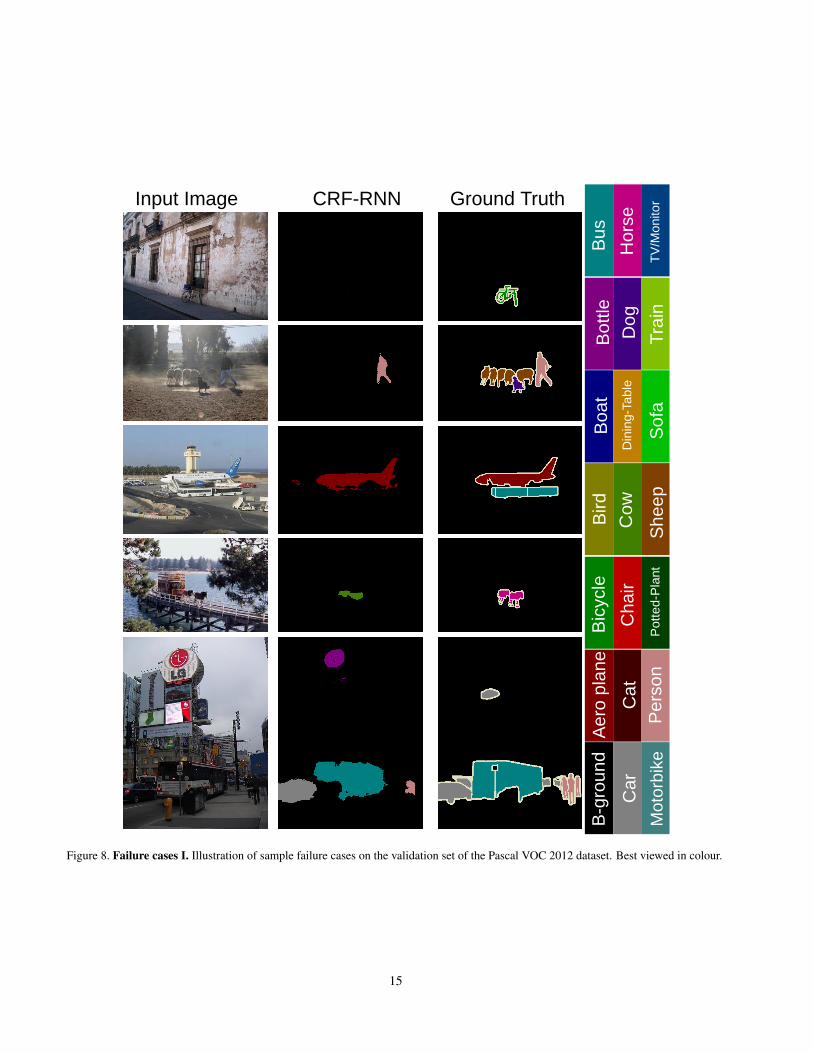
Figure 8. Failure cases I. Illustration of sample failure cases on the validation set of the Pascal VOC 2012 dataset. Best viewed in colour.

15

Input Image CRF-RNN Ground Truth

B-g

rou

nd

Ae

ro p

lan

eB

icycle

Bird

Bo

at

Bo

ttle

Bu

s

Ca

rC

at

Ch

air

Co

wD

inin

g-T

able

Do

gH

ors

e

Moto

rbik

eP

ers

on

Pott

ed-P

lant

Sh

ee

pS

ofa

Tra

inT

V/M

onitor

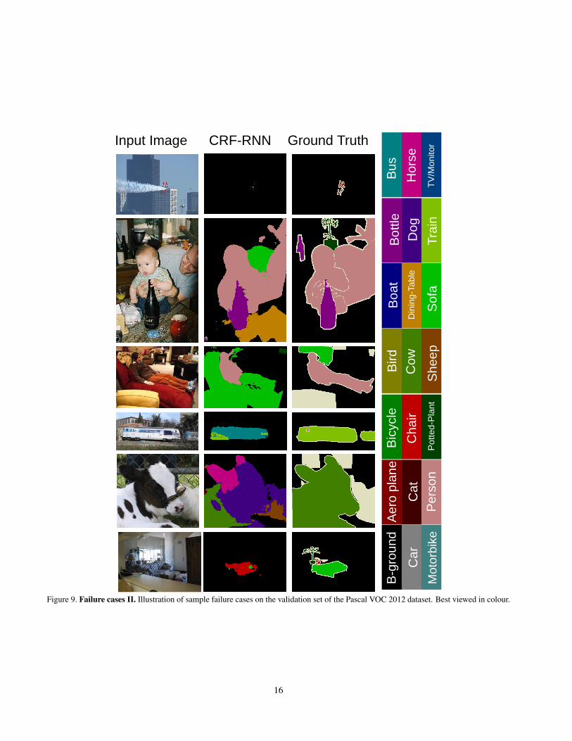
Figure 9. Failure cases II. Illustration of sample failure cases on the validation set of the Pascal VOC 2012 dataset. Best viewed in colour.

16

B-ground Aero plane Bicycle Bird Boat Bottle Bus

Car Cat Chair Cow Dinging-table Dog Horse

Motorbike Person Potted-Plant Sheep Sofa Train TV/Monitor

Input Image Ground TruthCRF-RNNDeepLabFCN-8s

B-ground Aero plane Bicycle Bird Boat Bottle Bus

Car Cat Chair Cow Dining-Table Dog Horse

Motorbike Person Potted-Plant Sheep Sofa Train TV/Monitor

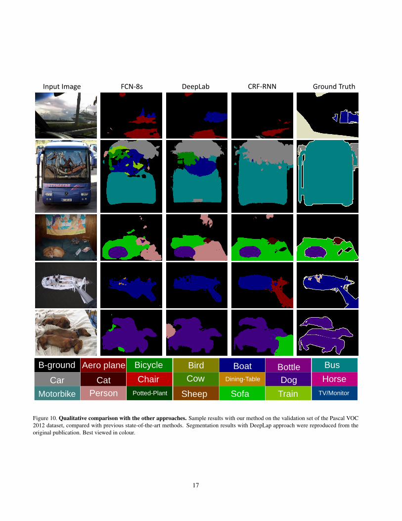
Figure 10. Qualitative comparison with the other approaches. Sample results with our method on the validation set of the Pascal VOC2012 dataset, compared with previous state-of-the-art methods. Segmentation results with DeepLap approach were reproduced from theoriginal publication. Best viewed in colour.

17