conditional mean-variance and mean-semivariance models in
TRANSCRIPT
HAL Id: hal-01404752https://hal.inria.fr/hal-01404752
Preprint submitted on 29 Nov 2016
HAL is a multi-disciplinary open accessarchive for the deposit and dissemination of sci-entific research documents, whether they are pub-lished or not. The documents may come fromteaching and research institutions in France orabroad, or from public or private research centers.
L’archive ouverte pluridisciplinaire HAL, estdestinée au dépôt et à la diffusion de documentsscientifiques de niveau recherche, publiés ou non,émanant des établissements d’enseignement et derecherche français ou étrangers, des laboratoirespublics ou privés.
Conditional Mean-Variance and Mean-Semivariancemodels in portfolio optimization
Hanene Salah, Ali Gannoun, Mathieu Ribatet
To cite this version:Hanene Salah, Ali Gannoun, Mathieu Ribatet. Conditional Mean-Variance and Mean-Semivariancemodels in portfolio optimization. 2016. �hal-01404752�
Conditional Mean-Variance and Mean-Semivariancemodels in portfolio optimization
Hanene Ben Salah
BESTMOD Laboratory, ISG 41 Rue de la Liberte, Cite Bouchoucha 2000 Le Bardo,Tunisie
IMAG 34095 Montpellier cedex 05
Universite de Lyon, Universite Claude Bernard Lyon 1, Institut de Science Financiere et
d’Assurances, LSAF EA2429, F-69366 Lyon, France
Ali Gannoun
IMAG 34095 Montpellier cedex 05
Christian de Peretti
Universite de Lyon, Universite Claude Bernard Lyon 1, Institut de Science Financiere et
d’Assurances, LSAF EA2429, F-69366 Lyon, France
Mathieu Ribatet
IMAG 34095 Montpellier cedex 05
Abstract
It is known that the historical observed returns used to estimate the expected
return provide poor guides to predict the future returns. Consequently, the op-
timal portfolio weights are extremely sensitive to the return assumptions used.
Getting information about the future evolution of different asset returns, could
help the investors to obtain more efficient portfolio. The solution will be reached
by estimating the portfolio risk by conditional variance or conditional semivari-
ance. This strategy allows us to take advantage of returns prediction which will
be obtained by nonparametric univariate methods. Prediction step uses kernel
estimation of conditional mean. Application on the Chinese and the American
markets are presented and discussed.
Keywords: Conditional Semivariance, Conditional Variance, DownSide Risk,
Kernel Method, Nonparametric Mean prediction.
Preprint submitted to Journal title November 26, 2016
1. Introduction1
Investment strategies and their profitability have always been a hot topic2
for people with an interest in financial assets. The modern asset allocation3
theory was originated from the Mean-Variance portfolio model introduced by4
Markowitz (1952), see also Markowitz (1959) and Markowitz (1990). The origi-5
nal Markowitz model simply dealt with the use of historical returns. Variance is6
commonly used as a risk measure in portfolio optimisation to find the trade-off7
between the risk and return. In practice, the expected returns and variances are8
calculated using historical data observed before the portfolio optimization date9
and are used as proxies for future returns.This practice is not purely guesswork,10
there are well-developed nonparametric approaches to obtain good forecasts.11
Markowitz’s portfolio optimization requires the knowledge of both the ex-12
pected return and the covariance matrix of the assets. It is well known that the13
optimum portfolio weights are very sensitive to return expectations which are14
very difficult to determine. For instance, historical returns are bad predictors15
of the future returns if we use the classical arithmetic mean (Michaud, 1989;16
Black and Litterman, 1992; Siegel and Woodgate, 2007). Estimating covariance17
matrices is a delicate statistical challenge that requires sophisticated methods18
(see Ledoit and Wolf (2004)). It is fair to state that, due to the large statistical19
errors of the input of Markowitz’s portfolio optimization, its result is not reli-20
able and should be considered very cautiously. This led Levy and Roll (2010)21
to turn the usual approach up-side-down and found that minor adjustments of22
the input parameter are much needed, well within the statistical uncertainties.23
There are various models to used in forecasting future financial time series.24
For example, Delatola and Griffin (2011) developed a prediction method based25
on Bayesian nonparametric modelling of the return distribution with stochastic26
volatility and Kresta (2015) proposed to use of a GARCH-copula model in27
Portfolio Optimization .28
In this paper, we propose a radical different methods by including infor-29
mations about the possible future returns in the estimation step obtained by30
2
kernel nonparametric prediction. Then, we can improve the quality of portfolio31
optimisation.32
Firstly, we exhibit the classical Markowitz model developed in 1952.33
Let us say that there are m assets to constitute a portfolio P and denote34
by rjt the return of asset j on date t, t = 1, . . . , N , and M the estimated35
variance-covariance matrix of the returns (r1, . . . , rm),36
M =1
N
N∑t=1
(r1t − r1)2 (r1t − r1)(r2t − r2) (r1t − r1)(rmt − rm)
(r2t − r2)(r1t − r1) (r2t − r2)2 (r2t − r2)(rmt − rm)...
......
(rmt − rm)(r1t − r1) (rmt − rn)(r2t − r2) (rmt − rm)2
.(1)
The optimization program is then the following37
minω
ω>Mω, subject to ω>µ = E∗, ω>1 = 1, (2)
where ω> = (ω1, . . . , ωm) is the portfolio vector weight, µ> = (r1, . . . , rm) =38
( 1N
∑Nt=1 r1t, . . . ,
1N
∑Nt=1 rmt) the empirical mean returns and E∗ is a target39
expected portfolio return.40
Using Lagrangian method, the explicit solution of solution of (2) is :41
ω∗ =αE∗ − λαθ − λ2
M−1µ+θ − λE∗
αθ − λ2M−11, (3)
where α = 1>M−11, λ = µ>M−11 and θ = µ>M−1µ.42
This model depends strictly on the assumptions that the assets returns follow43
normal distribution and investor has quadratic utility function. However, these44
two conditions are not checked. Many researchers have showed that the assets45
returns distribution are asymmetric and exhibit skewness, see Tobin (1958);46
Arditti (1971); Chunhachinda et al. (1997); Prakash et al. (2003). These authors47
have proposed a DownSide Risk (DSR) measures such as Semivariance (SV)48
and conditional value at risk (CVaR). These DSR measures are consistent with49
investor’s perception towards risk as they focus on return dispersions below50
3
any benchmark return B chosen by the investor. Below, we focus only on the51
Semivariance risk measure which is often considered as a more plausible risk52
one than the variance. The associated optimization program is the following:53
minω
ω>MSRω subject to ω>µ = E∗, ω>1 = 1, (4)
where MSR is the matrix with coefficients54
ΣijB =1
N
V∑t=1
(rit −B)(rjt −B)
such that V is the period in which the portfolio underperforms the target return55
B.56
The major obstacle to get the solution of this problem is that the semico-57
variance matrix is endogenous (see Estrada (2004, 2008)), that is, the change in58
weights affects the periods in which the portfolio underperforms the target rate59
of return, which in turn affects the elements of the Semivariance matrix.60
Many authors propose different methods to estimate the elements of MSR in61
order to resolve problem defined in equation (4). Among them, Hogan and War-62
ren (1974) propose to use the Frank-Wolf algorithm but the main disadvantage63
of this algorithm is its slow convergence rate. Moreover, during early iteration,64
this algorithm tends to decrease the objective function. Ang (1975) proposes to65
linearise the Semivariance so that the optimization problem can be solved using66
linear programming. However, this method ignores the inter-correlations be-67
tween securities. Harlow (1991) also considers problem (4) and generates Mean-68
Semivariance efficient frontier, which he compares to the Mean-Variance effi-69
cient frontier. Mamoghli and Daboussi (2008) improve Harlow approach. Their70
model permits to surmount the problem of inequality of the Semicovariance71
measures which occurs in the Mean-Semivariance model of Harlow. Markowitz72
et al. (1993) transform the Mean-Semivariance problem into a quadratic problem73
by adding fictitious securities. Estrada (2008) proposes a simple and accurate74
heuristic approach that yields a symmetric and exogenous Semicovariance ma-75
trix, which enables the determination of Mean-Semivariance optimal portfolios76
4

by using the well-known closed-form solutions of Mean-Variance problems. In77
Athayde (2001) and (Athayde, 2003), there is an iterative algorithm which is78
used to construct a Mean-DownSide Risk portfolio frontier. This algorithm is79
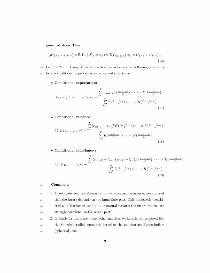
improved by Ben Salah et al. (2016a) and Ben Salah et al. (2016b) by intro-80
ducing nonparametric estimation of the returns in order to get a better smooth81
efficient frontier.82
A knowledgeable investor should have an overview on market development.83
For a fixed amount to invest now, he has to predict, day by day (or month by84
month, . . . ), the optimal return that his investment could bring to him.85
In this paper, we will develop a rule of decision to optimize the portfolio86
selection through reducing the risk calculated using the classical variance. A87
new approach, called conditional Markowitz optimization method, will be used88
to determine an optimal portfolio. This portfolio is obtained by minimizing89
the so-called conditional risk. This risk may in turn be broken down into two90
versions: Mean-Variance and Mean-Semivariance approaches. The main idea is91
to anticipate the values of the assets returns on the date N + 1 (knowing the92
past) and incorporate this information in the optimization model.93
The rest of the article is organized as follows. Section 2 introduces the non-94
parametric conditional risk. We start by giving an overview on nonparametric95
regression and prediction, as well as conditional variance and covariance defini-96
tions. The conditional Mean-Variance and the conditional Mean-Semivariance97
models are exhibited in this Section. Numerical studies based on the Chinese98
and the American Market dataset are presented in Section 3. The last Section99
is devoted to conclusion and further development.100
2. Nonparametric Conditional Risk101
Here, we start by giving some general concepts and results concerning non-102
parametric regression and prediction. Then, we define the Conditional Mean-103
Variance and Mean-Semivariance models and we exhibit the corresponding al-104
gorithms to get the optimal portfolio.105
5
2.1. Nonparametric Regression Model106
In the following subsection, we outline the mechanics of kernel regression107
estimation.108
Let (X,Y ) be a pair of explanatory and response random variables with
joint density f(x, y), and )(Yi, Xi)i=1,T T -copies of (X,Y ). We suppose that X
is m-dimensional. Using a quadratic criterion, the best prediction of Y based
on X = x is the conditional expectation E(Y | X = x) = g(x).
Using (Yi, Xi)i=1,T , we will focus on the estimation of the unknown mean re-
sponse g(x).
The regression model is
Yt = g(xt) + εt, (5)
where g(.) is unknown. The errors εt satisfy
E(εt) = 0, V (εt) = σ2ε , Cov(εi, εj) = 0 for i 6= j. (6)
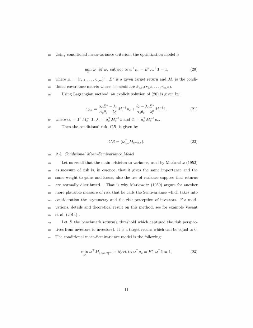
To derive the estimator note that we can express g(x) in terms of the joint
probability density function f(x, y) as follows:
g(x) = E(Y | X = x) =
∫yf(y | x)dy =
∫yf(x, y)dy∫f(x, y)dy
(7)
Using kernel density estimation of the joint distribution and the marginal one
(see (Bosq and Lecoutre, 1987)), the Nadaraya-Watson estimator for g(x) is
given by :
g(x) =
T∑t=1
YtKH(Xt − x)
T∑t=1KH(Xt − x)
(8)
where KH(x) = |H|−1/2K(|H|−1/2x) with H is the m×m matrix of smoothing
parameters which is symmetric and positive definite and |H| its determinant.
The function K : Rm → [0,∞) is a probability density.
By the way, the conditional variance is given by
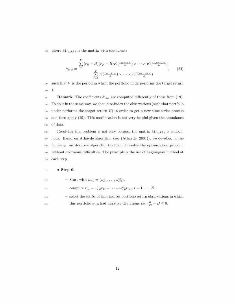
σ2(x) = E((Y − g(x))2 | X = x), (9)
6
and its kernel estimator is given by
σ2(x) =
T∑t=1
(Yt − ˆg(x))2KH(Xt − x)
T∑t=1KH(Xt − x)
. (10)
If Y = (Y1, . . . , Ym) is a random vector, the conditional covariance between Y1
and Y2 given X = x is defined as
σ12(x) = E(Y1 − g1(x))(Y2 − g2(x)) | X = x), (11)
and its kernel estimator is given by
σ12(x) =
T∑t=1
(Y1t − g1(x))(Y2t − g2(x))KH(Xt − x)
T∑t=1KH(Xt − x)
, (12)
where g1(x) and g1(x) (respectively g2(x) and g2(x)) are the E(Y1 | X = x) and109
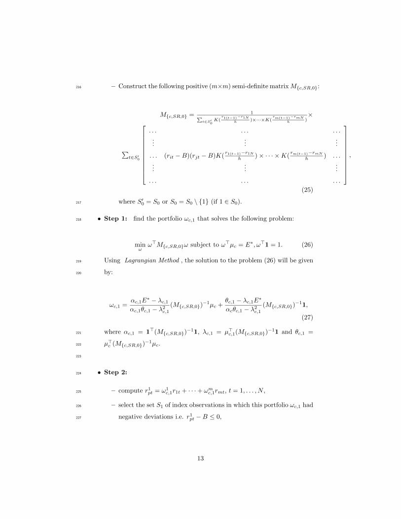
its kernel estimator (respectively the E(Y1 | X = x) and its kernel estimator)110
defined above.111
112
The choice of the bandwidth matrix H is the most important factor affecting113
the accuracy of the estimator (8), since it controls the orientation and amount114
of smoothing induced.115
The simplest choice for this matrix is to take H = hIm, where h is a unidi-116
mensional smoothing parameter and Im is the m×m identity matrix. Then we117
have the same amount of smoothing applied in all coordinate directions and the118
kernel estimator (8) has the form119
g(x) =
T∑t=1
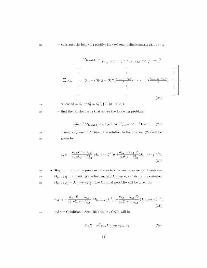
YtK(Xt−xh )
T∑t=1K(Xt−x
h )
=
T∑t=1
YtKh(Xt − x)
T∑t=1Kh(Xt − x)
, (13)
where Kh(x) = h−mK(xh ). The estimators (10) and (12) are derived similarly.120
Another choice, relatively easy-to-manage, is to take the bandwidth matrix121
equal to a diagonal matrix, which allows for different amounts of smoothing in122
7
each of the coordinates.123
The following kernel functions are used most often in multivariate nonparametric124
estimation:125
• product kernel: K(x) = K(x1)× · · · ×K(xm) =∏mj=1 k(xj) where k(.) is126
an univariate density function.127
• symmetric kernel: Ck,mk(‖x‖1/22 ).128
The multivariate Gaussian density K(x) = (2π)−m/2exp(x>x2 ) is a product and129
symmetric kernel.130
In the rest of this paper, we will consider only the product kernel and the131
bandwidth matrix H = diag(h1, . . . , hm). Then, for x = (x1, . . . , xm), the132
estimator (8) should be written as follows:133
g(x) =
T∑t=1
Ytk(X1t−x1
h1)× · · · × k(Xmt−xm
hm)
T∑t=1
k(X1t−x1
h1)× · · · × k(Xmt−xm
hm)
, (14)
with hj = T−1/m+4σj where σj is an estimator of the standard deviation of the134
random variable Xj . These bandwidths are optimal using the minimisation of135
the Asymmetrical Mean Integrated Error criterion (see for example (Wasserman,136
2006)).137
The estimators (10) and (12) are derived similarly.138
2.2. Nonparametric Prediction139
Nonparametric smoothing techniques can be applied beyond the estimation
of the autoregression function. Consider a m-multivariate stationary time series
{(r1t, . . . , rmt), t = 1, . . . , N}. We consider the processes (Xt, Yt) defined as
follows
Xt = (r1t, . . . , rmt) Yt = rj(t+1), (15)
and we are interested in predicting the return of a given asset j on time N + 1.
This problem is equivalent to the estimation of the regression g(.) function
8
presented above. Then
g(r1N , . . . , rmN ) = E(YN | XN = xN ) = E(rj(N+1) | xN = (r1N , . . . , rmN )).
(16)
Let T = N − 1. Using the kernel method, we get easily the following estimators140
for the conditional expectation, variance and covariance:141
• Conditional expectation:
rc,j = g(r1N , . . . ,= rmN ) =
T∑t=1
rj(t+1)K( r1t−r1Nh )× · · · ×K( rmt−rmN
h )
T∑t=1
K( r1t−r1Nh )× · · · ×K( rmt−rmN
h )
,
(17)
• Conditional variance :
σ2c,j(r1N , . . . , rmN ) =
T∑t=1
(rj(t+1) − rc,j)2K( r1t−r1Nh )× · · · ×K( rmt−rmN
h )
T∑t=1
K( r1t−r1Nh )× · · · ×K( rmt−rmN
h )
,
(18)
• Conditional covariance :
σc,ij(r1N , . . . , rmN ) =
T∑t=1
(ri(t+1) − rc,i)(rj(t+1) − rc,j)K( r1t−r1Nh )× · · · ×K( rmt−rmN
h )
T∑t=1
K( r1t−r1Nh )× · · · ×K( rmt−rmN
h )
,
(19)
Comments142
1. To estimate conditional expectation, variance and covariance, we supposed143
that the future depends on the immediate past. This hypothesis, consid-144
ered as 1-Markovian condition, is natural because the future returns are145
strongly correlated to the recent past.146
2. In Statistics literature, many other multivariate kernels are proposed like147
the Spherical/radial-symmetric kernel or the multivariate Epanechnikov148
(spherical) one.149
9

3. Nonparametric methods are typically indexed by a bandwidth or tuning150
parameter which controls the degree of complexity. The choice of band-151
width is often critical to implementation: under- or over-smoothing can152
substantially reduce precision. The standard approach to the bandwidth153
problem is to choose a bandwidth that minimizes some measures of global154
risk for the entire regression function, usually Mean Integrated Squared155
Error (MISE), i.e. the expected squared error integrated over the entire156
curve. The optimal bandwidth is then estimated either using plug-in es-157
timators of the minimizer of the asymptotic approximation to MISE or158
using an unbiased data-based estimator of the MISE . This is the cross-159
validation method. This method was analyzed in Sarda (1993). It is160
recommended by (Altman and Leger, 1995) when large samples are avail-161
able. As to the estimation of the conditional covariance matrix, one may162
use different bandwidths for different elements of this matrix. However,163
the resulting estimation with different bandwidths cannot be guaranteed164
to be positive definite (Li et al. (2007) ). In practice, the positive definite-165
ness is a desirable property. Thus, we suggest using the same bandwidth166
for all elements.167
2.3. Conditional Mean-Variance Model168
Our goal here is to constitute an optimal portfolio using conditional criterion.169
In our opinion, it is natural to use conditional information to provide a timely170
and effective solution.171
We suppose that they are, as in the previous section, m assets to be used172
for constructing a well diversified portfolio. Optimizing asset allocation is sim-173
ply defined as the process of mixing asset weights of a portfolio within the174
constraints of an investor’s capital resources to yield the most favourable risk-175
return trade-off. The risk here is defined by the conditional variance of ,the176
portfolio return.177
Let ω = (ω1, . . . , ωm)> be the portfolio weight vector and rpt = ω1r1t +178
ω2r2t + ... + ωmrmt, t = 1 . . . , N , N -realisations of the the portfolio return Rp.179
10
Using conditional mean-variance criterion, the optimization model is180
minω
ω>Mcω, subject to ω>µc = E∗, ω>1 = 1, (20)
where µc = (rc,1, . . . , rc,m)>, E∗ is a given target return and Mc is the condi-181
tional covariance matrix whose elements are σc,ij(r1N , . . . , rmN ).182
Using Lagrangian method, an explicit solution of (20) is given by:183
ωc,∗ =αcE
∗ − λcαcθc − λ2c
M−1c µc +θc − λcE∗
αcθc − λ2cM−1c 1, (21)
where αc = 1>M−1c 1, λc = µ>c M−1c 1 and θc = µ>c M
−1c µc.184
Then the conditional risk, CR, is given by185
CR = (ω>c,∗Mcωc,∗). (22)
2.4. Conditional Mean-Semivariance Model186
Let us recall that the main criticism to variance, used by Markowitz (1952)187
as measure of risk is, in essence, that it gives the same importance and the188
same weight to gains and losses, also the use of variance suppose that returns189
are normally distributed . That is why Markowitz (1959) argues for another190
more plausible measure of risk that he calls the Semivariance which takes into191
consideration the asymmetry and the risk perception of investors. For moti-192
vations, details and theoretical result on this method, see for example Vasant193
et al. (2014) .194
Let B the benchmark return(a threshold which captured the risk perspec-195
tives from investors to investors). It is a target return which can be equal to 0.196
The conditional mean-Semivariance model is the following:197
minω
ω>M{c,SR}ω subject to ω>µc = E∗, ω>1 = 1, (23)
11
where M{c,SR} is the matrix with coefficients198
σijB =
V∑t=1
(rit −B)(rjt −B)K( r1t−r1Nh )× · · · ×K( rmt−rmN
h )
V∑t=1
K( r1t−r1Nh )× · · · ×K( rmt−rmN
h )
, (24)
such that V is the period in which the portfolio underperforms the target return199
B.200
Remark. The coefficients σijB are computed differently of those from (19).201
To do it in the same way, we should re-index the observations (such that portfolio202
under performs the target return B) in order to get a new time series process203
and then apply (19). This modification is not very helpful given the abundance204
of data.205
Resolving this problem is not easy because the matrix M{c,SR} is endoge-206
nous. Based on Athayde algorithm (see (Athayde, 2001)), we develop, in the207
following, an iterative algorithm that could resolve the optimization problem208
without enormous difficulties. The principle is the use of Lagrangian method at209
each step.210
• Step 0:211
– Start with ωc,0 = (ω1c,0, . . . , ω
mc,0),212
– compute r0pt = ω1c,0r1t + · · ·+ ωmc,0rmt, t = 1, . . . , N ,213
– select the set S0 of time indices portfolio return observations in which214
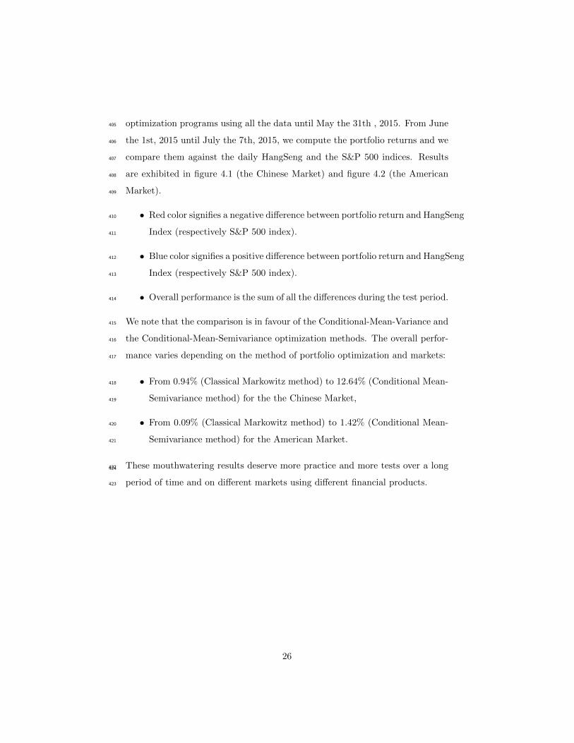
this portfolio ωc,0 had negative deviations i.e. r0pt −B ≤ 0.215
12
– Construct the following positive (m×m) semi-definite matrixM{c,SR,0}:216
M{c,SR,0} = 1∑t∈S′0
K(r1(t−1)−r1N
h )×···×K(rm(t−1)−rmN
h )×
∑t∈S′0
. . . . . . . . ....
......
. . . (rit −B)(rjt −B)K(r1(t−1)−r1N
h )× · · · ×K(rm(t−1)−rmN
h ) . . ....
......
. . . . . . . . .
,
(25)
where S′0 = S0 or S0 = S0 \ {1} (if 1 ∈ S0).217
• Step 1: find the portfolio ωc,1 that solves the following problem:218
minω
ω>M{c,SR,0}ω subject to ω>µc = E∗, ω>1 = 1. (26)
Using Lagrangian Method , the solution to the problem (26) will be given219
by:220
ωc,1 =αc,1E
∗ − λc,1αc,1θc,1 − λ2c,1
(M{c,SR,0})−1µc +
θc,1 − λc,1E∗
αcθc,1 − λ2c,1(M{c,SR,0})
−11,
(27)
where αc,1 = 1>(M{c,SR,0})−11, λc,1 = µ>c,1(M{c,SR,0})
−11 and θc,1 =221
µ>c (M{c,SR,0})−1µc.222
223
• Step 2:224
– compute r1pt = ω1c,1r1t + · · ·+ ωmc,1rmt, t = 1, . . . , N ,225
– select the set S1 of index observations in which this portfolio ωc,1 had226
negative deviations i.e. r1pt −B ≤ 0,227
13
– construct the following positive (m×m) semi-definite matrixM{c,SR,1}:228
M{c,SR,1} = 1∑t∈S′1
K(r1(t−1)−r1N
h )×···×K(rm(t−1)−rmN
h )×
∑t∈S1
. . . . . . . . ....
......
. . . (rit −B)(rjt −B)K(r1(t−1)−r1N
h )× · · · ×K(rm(t−1)−rmN
h ) . . ....
......
. . . . . . . . .
,
(28)
where S′1 = S1 or S′1 = S1 \ {1} (if 1 ∈ S1).229
– find the portfolio ωc,2 that solves the following problem:230
minω
ω>M{c,SR,1}ω subject to ω>µc = E∗, ω>1 = 1. (29)
Using Lagrangian Method , the solution to the problem (29) will be231
given by:232
ωc,2 =αc,2E
∗ − λc,2αc,2θc,2 − λ2c,2
(M{c,SR,1})−1µc+
θc,2 − λc,2E∗
αcθc,2 − λ2c,2(M{c,SR,1})
−11.
(30)
• Step 3: iterate the previous process to construct a sequence of matrices233
M{c,SR,l} until getting the first matrix M{c,SR,F} satisfying the criterion234
M{c,SR,F} = M{c,SR,F+1}. The Optimal portfolio will be given by:235
ωc,F+1 =αc,FE
∗ − λc,Fαc,F θc,F − λ2c,F
(M{c,SR,F})−1µc+
θc,F − λc,FE∗
αcθc,F − λ2c,F(M{c,SR,F})
−11.
(31)
and the Conditional Semi Risk value , CSR, will be236
CSR = ω>c,F+1M{c,SR,F}ωc,F+1 (32)
14
Remarks.237
1. There is a finite number of iterations to get the optimal solution.238
2. In the prediction step (to get the an unobservable values of the returns),239
we treated separately the evolution of each asset. It is possible to make240
multivariate (or vectorial) prediction and get jointly the unobservable val-241
ues for all the assets.242
3. Short selling is allowed in this model, i.e. the optimal portfolio can have243
a negative weight for some assets. To forbid short selling, the additional244
constraint ωj ≥ 0 for j = 1, . . . ,m is necessary.245
3. Empirical Analysis246
In this section, the performance of the conditional mean-variance and the247
conditional mean-semivariance optimisation methods are investigated. They are248
compared to Classical Markowitz and DownSide methods. It is supposed that249
there is no transaction costs, no taxes and that the benchmark B = 0.250
3.1. Data251
A dataset, drawn from Reuters, was used for this analysis. The original252
Data are a daily stock returns belonged to two markets:253
• The Chinese market (emerging market) with 16 assets. They are 897254
daily observations (returns) for each asset from November the 14th, 2011,255
to July 8th, 2015,256
• The American market (developed market) with 19 assets. They are 788257
daily observations (returns) for each asset from June, 18th, 2012 to July,258
8th, 2015.259
To compare the efficiency and the performance of the proposed methods, we use260
the daily values of261
15
• The Hang Seng Index-HSI that aims to capture the leadership of the262
Hong Kong exchange, and covers approximately 65% of its total market263
capitalization,264
• The S&P 500 Index that tracks 500 large U.S. companies across a wide265
span of industries and sectors. The stocks in the S&P 500 represent266
roughly 70 % of all the stocks that are publicly traded.267
The assets returns are calculated from stock prices observed on Thomson Reuters268
Platform as follows:269
rt =pt − pt−1pt−1
, (33)
with270
• pt: Stock price at date t,271
• pt−1: Stock price at date t− 1272
The prices pt, t = 1, . . . , N ; are adjusted for dividends.273
The historical statistics of the asset markets are summarised below.274
3.2. Historical statistics275
In this subsection, historical statistics are proposed. The goal is to check276
the normality or not of the returns distribution in order to decide which risk277
measure is more appropriate to determine the optimal portfolio.278
3.2.1. The Chinese Market279
Let us start by the Chinese Market. Over the past two decades, the Chinese280
economy and financial markets have undergone a remarkable transformation281
and have seen significant growth. More specifically, the Chinese equity market282
has grown from a once very rudimentary and closed market to one of the largest283
equity markets in the world. Although most of the Chinese equity market still284
remains in the hands of controlling parties and domestic investors, authorities285
have made significant progress in opening the market to foreign capital and286
16
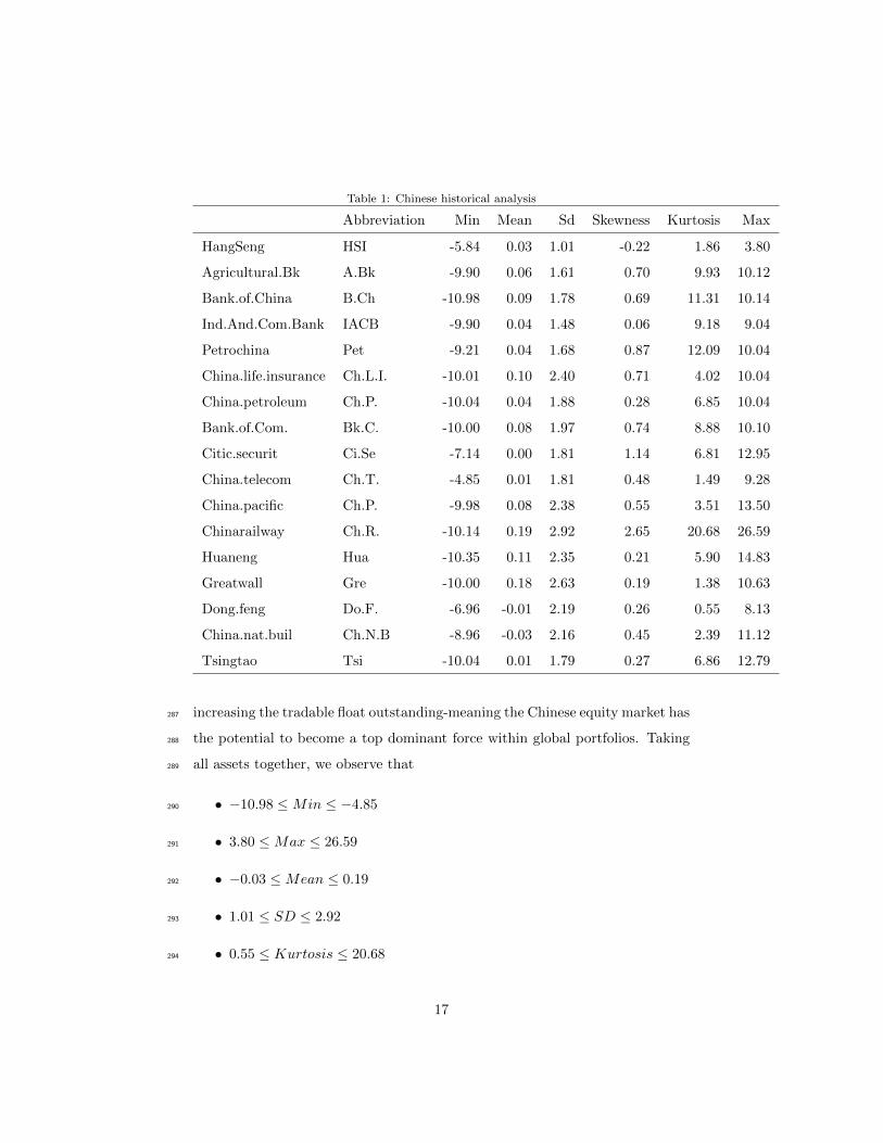
Table 1: Chinese historical analysis
Abbreviation Min Mean Sd Skewness Kurtosis Max
HangSeng HSI -5.84 0.03 1.01 -0.22 1.86 3.80
Agricultural.Bk A.Bk -9.90 0.06 1.61 0.70 9.93 10.12
Bank.of.China B.Ch -10.98 0.09 1.78 0.69 11.31 10.14
Ind.And.Com.Bank IACB -9.90 0.04 1.48 0.06 9.18 9.04
Petrochina Pet -9.21 0.04 1.68 0.87 12.09 10.04
China.life.insurance Ch.L.I. -10.01 0.10 2.40 0.71 4.02 10.04
China.petroleum Ch.P. -10.04 0.04 1.88 0.28 6.85 10.04
Bank.of.Com. Bk.C. -10.00 0.08 1.97 0.74 8.88 10.10
Citic.securit Ci.Se -7.14 0.00 1.81 1.14 6.81 12.95
China.telecom Ch.T. -4.85 0.01 1.81 0.48 1.49 9.28
China.pacific Ch.P. -9.98 0.08 2.38 0.55 3.51 13.50
Chinarailway Ch.R. -10.14 0.19 2.92 2.65 20.68 26.59
Huaneng Hua -10.35 0.11 2.35 0.21 5.90 14.83
Greatwall Gre -10.00 0.18 2.63 0.19 1.38 10.63
Dong.feng Do.F. -6.96 -0.01 2.19 0.26 0.55 8.13
China.nat.buil Ch.N.B -8.96 -0.03 2.16 0.45 2.39 11.12
Tsingtao Tsi -10.04 0.01 1.79 0.27 6.86 12.79
increasing the tradable float outstanding-meaning the Chinese equity market has287
the potential to become a top dominant force within global portfolios. Taking288
all assets together, we observe that289
• −10.98 ≤Min ≤ −4.85290
• 3.80 ≤Max ≤ 26.59291
• −0.03 ≤Mean ≤ 0.19292
• 1.01 ≤ SD ≤ 2.92293
• 0.55 ≤ Kurtosis ≤ 20.68294
17
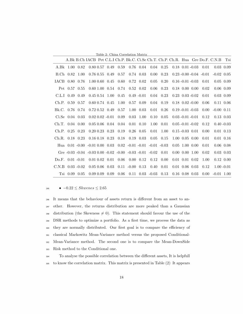
Table 2: China Correlation Matrix
A.Bk B.Ch IACB Pet C.L.I Ch.P. Bk.C. Ci.Se Ch.T. Ch.P. Ch.R. Hua Gre Do.F. C.N.B Tsi
A.Bk 1.00 0.82 0.80 0.57 0.49 0.59 0.76 0.04 0.04 0.25 0.18 0.01 -0.03 0.01 0.03 0.09
B.Ch 0.82 1.00 0.76 0.55 0.49 0.57 0.74 0.03 0.00 0.23 0.23 -0.00 -0.04 -0.01 -0.02 0.05
IACB 0.80 0.76 1.00 0.60 0.45 0.60 0.72 0.02 0.05 0.20 0.16 -0.01 -0.03 0.01 0.05 0.09
Pet 0.57 0.55 0.60 1.00 0.54 0.74 0.52 0.02 0.06 0.23 0.18 0.00 0.00 0.02 0.06 0.09
C.L.I 0.49 0.49 0.45 0.54 1.00 0.45 0.49 -0.01 0.04 0.23 0.23 0.03 -0.02 0.01 0.03 0.09
Ch.P. 0.59 0.57 0.60 0.74 0.45 1.00 0.57 0.09 0.04 0.19 0.18 0.02 -0.00 0.06 0.11 0.06
Bk.C. 0.76 0.74 0.72 0.52 0.49 0.57 1.00 0.03 0.01 0.26 0.19 -0.01 -0.03 0.00 -0.00 0.11
Ci.Se 0.04 0.03 0.02 0.02 -0.01 0.09 0.03 1.00 0.10 0.05 0.03 -0.01 -0.01 0.12 0.13 0.03
Ch.T. 0.04 0.00 0.05 0.06 0.04 0.04 0.01 0.10 1.00 0.01 0.05 -0.01 -0.02 0.12 0.40 -0.03
Ch.P. 0.25 0.23 0.20 0.23 0.23 0.19 0.26 0.05 0.01 1.00 0.15 -0.03 0.01 0.00 0.01 0.13
Ch.R. 0.18 0.23 0.16 0.18 0.23 0.18 0.19 0.03 0.05 0.15 1.00 0.05 0.00 0.01 0.01 0.16
Hua 0.01 -0.00 -0.01 0.00 0.03 0.02 -0.01 -0.01 -0.01 -0.03 0.05 1.00 0.00 0.01 0.06 0.08
Gre -0.03 -0.04 -0.03 0.00 -0.02 -0.00 -0.03 -0.01 -0.02 0.01 0.00 0.00 1.00 0.02 0.03 0.03
Do.F. 0.01 -0.01 0.01 0.02 0.01 0.06 0.00 0.12 0.12 0.00 0.01 0.01 0.02 1.00 0.12 0.00
C.N.B 0.03 -0.02 0.05 0.06 0.03 0.11 -0.00 0.13 0.40 0.01 0.01 0.06 0.03 0.12 1.00 -0.01
Tsi 0.09 0.05 0.09 0.09 0.09 0.06 0.11 0.03 -0.03 0.13 0.16 0.08 0.03 0.00 -0.01 1.00
• −0.22 ≤ Skwenes ≤ 2.65295
It means that the behaviour of assets return is different from an asset to an-296
other. However, the returns distribution are more peaked than a Gaussian297
distribution (the Skewness 6= 0). This statement should favour the use of the298
DSR methods to optimize a portfolio. As a first time, we process the data as299
they are normally distributed. Our first goal is to compare the efficiency of300
classical Markowitz Mean-Variance method versus the proposed Conditional-301
Mean-Variance method. The second one is to compare the Mean-DownSide302
Risk method to the Conditional one.303
To analyse the possible correlation between the different assets, It is helpfull304
to know the correlation matrix. This matrix is presented in Table (2) It appears305
18

that the returns are differently correlated between each other. For example,306
Agricultural.Bk is strongly correlated to Bank.of.China and Ind.And.Com.Bank307
assets, and very weakly correlated to Dong.feng and China.nat.buil assets. More308
generally, the correlation between two stocks is larger when they are from bank-309
ing sector than when they belong to different industries. The use of Principal310
Component Analysis (PCA) could reduce the number of assets to constitute the311
optimal portfolio. This step is omitted in this paper.312
Remark.313
In this matrix, we have excluded, the correlation between the HangSeng314
Index and the other assets because we will use it as a benchmark to compare315
its return to the optimal portfolio’s.316
3.2.2. The Americain Market317
As for the Chinese Market, similar historical statistics are done for the Amer-318
ican one. In the beginning, we display and comment the descriptive statistics,319
then we exhibit and comment the correlation matrix.320
Taking all assets together, we observe that321
• −14.34 ≤Min ≤ −0.90322
• 2.54 ≤Max ≤ 29.56323
• 0.0 ≤Mean ≤ 0.21324
• 0.73 ≤ SD ≤ 2.73325
• 0.85 ≤ Kurtosis ≤ 21.88326
• −0.54 ≤ Skwenes ≤ 2.18327
The behaviour of assets return is different from an asset to another. However,328
most of distributions are more peaked than a Gaussian distribution (the Skew-329
ness 6= 0). The SP 500 index could being considered as normally distributed330
(Skewness=-0.15 , Kurtosis=0.99).331
Table (4) is devoted to the Correlation Matrix:332
19
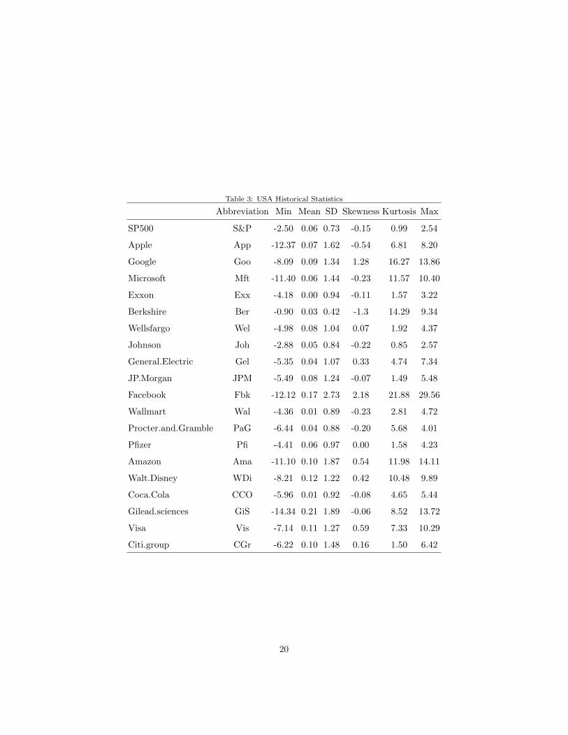
Table 3: USA Historical Statistics
Abbreviation Min Mean SD Skewness Kurtosis Max
SP500 S&P -2.50 0.06 0.73 -0.15 0.99 2.54
Apple App -12.37 0.07 1.62 -0.54 6.81 8.20
Google Goo -8.09 0.09 1.34 1.28 16.27 13.86
Microsoft Mft -11.40 0.06 1.44 -0.23 11.57 10.40
Exxon Exx -4.18 0.00 0.94 -0.11 1.57 3.22
Berkshire Ber -0.90 0.03 0.42 -1.3 14.29 9.34
Wellsfargo Wel -4.98 0.08 1.04 0.07 1.92 4.37
Johnson Joh -2.88 0.05 0.84 -0.22 0.85 2.57
General.Electric Gel -5.35 0.04 1.07 0.33 4.74 7.34
JP.Morgan JPM -5.49 0.08 1.24 -0.07 1.49 5.48
Facebook Fbk -12.12 0.17 2.73 2.18 21.88 29.56
Wallmart Wal -4.36 0.01 0.89 -0.23 2.81 4.72
Procter.and.Gramble PaG -6.44 0.04 0.88 -0.20 5.68 4.01
Pfizer Pfi -4.41 0.06 0.97 0.00 1.58 4.23
Amazon Ama -11.10 0.10 1.87 0.54 11.98 14.11
Walt.Disney WDi -8.21 0.12 1.22 0.42 10.48 9.89
Coca.Cola CCO -5.96 0.01 0.92 -0.08 4.65 5.44
Gilead.sciences GiS -14.34 0.21 1.89 -0.06 8.52 13.72
Visa Vis -7.14 0.11 1.27 0.59 7.33 10.29
Citi.group CGr -6.22 0.10 1.48 0.16 1.50 6.42
20
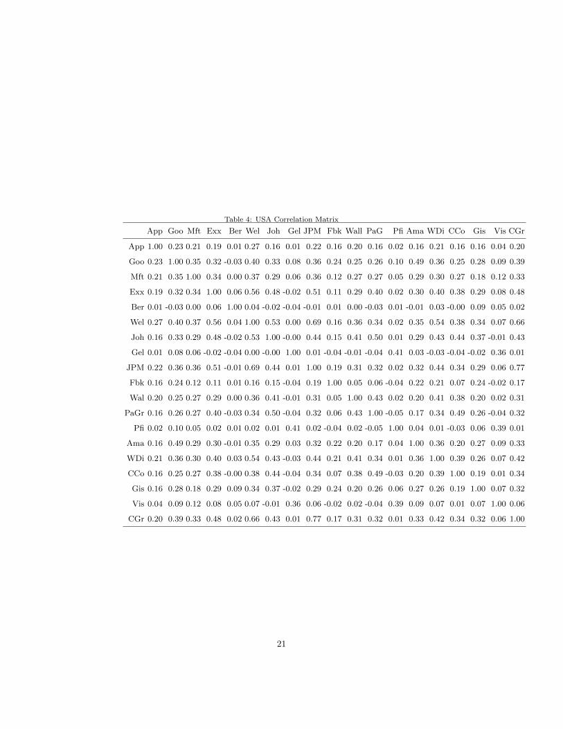
Table 4: USA Correlation Matrix
App Goo Mft Exx Ber Wel Joh Gel JPM Fbk Wall PaG Pfi Ama WDi CCo Gis Vis CGr
App 1.00 0.23 0.21 0.19 0.01 0.27 0.16 0.01 0.22 0.16 0.20 0.16 0.02 0.16 0.21 0.16 0.16 0.04 0.20
Goo 0.23 1.00 0.35 0.32 -0.03 0.40 0.33 0.08 0.36 0.24 0.25 0.26 0.10 0.49 0.36 0.25 0.28 0.09 0.39
Mft 0.21 0.35 1.00 0.34 0.00 0.37 0.29 0.06 0.36 0.12 0.27 0.27 0.05 0.29 0.30 0.27 0.18 0.12 0.33
Exx 0.19 0.32 0.34 1.00 0.06 0.56 0.48 -0.02 0.51 0.11 0.29 0.40 0.02 0.30 0.40 0.38 0.29 0.08 0.48
Ber 0.01 -0.03 0.00 0.06 1.00 0.04 -0.02 -0.04 -0.01 0.01 0.00 -0.03 0.01 -0.01 0.03 -0.00 0.09 0.05 0.02
Wel 0.27 0.40 0.37 0.56 0.04 1.00 0.53 0.00 0.69 0.16 0.36 0.34 0.02 0.35 0.54 0.38 0.34 0.07 0.66
Joh 0.16 0.33 0.29 0.48 -0.02 0.53 1.00 -0.00 0.44 0.15 0.41 0.50 0.01 0.29 0.43 0.44 0.37 -0.01 0.43
Gel 0.01 0.08 0.06 -0.02 -0.04 0.00 -0.00 1.00 0.01 -0.04 -0.01 -0.04 0.41 0.03 -0.03 -0.04 -0.02 0.36 0.01
JPM 0.22 0.36 0.36 0.51 -0.01 0.69 0.44 0.01 1.00 0.19 0.31 0.32 0.02 0.32 0.44 0.34 0.29 0.06 0.77
Fbk 0.16 0.24 0.12 0.11 0.01 0.16 0.15 -0.04 0.19 1.00 0.05 0.06 -0.04 0.22 0.21 0.07 0.24 -0.02 0.17
Wal 0.20 0.25 0.27 0.29 0.00 0.36 0.41 -0.01 0.31 0.05 1.00 0.43 0.02 0.20 0.41 0.38 0.20 0.02 0.31
PaGr 0.16 0.26 0.27 0.40 -0.03 0.34 0.50 -0.04 0.32 0.06 0.43 1.00 -0.05 0.17 0.34 0.49 0.26 -0.04 0.32
Pfi 0.02 0.10 0.05 0.02 0.01 0.02 0.01 0.41 0.02 -0.04 0.02 -0.05 1.00 0.04 0.01 -0.03 0.06 0.39 0.01
Ama 0.16 0.49 0.29 0.30 -0.01 0.35 0.29 0.03 0.32 0.22 0.20 0.17 0.04 1.00 0.36 0.20 0.27 0.09 0.33
WDi 0.21 0.36 0.30 0.40 0.03 0.54 0.43 -0.03 0.44 0.21 0.41 0.34 0.01 0.36 1.00 0.39 0.26 0.07 0.42
CCo 0.16 0.25 0.27 0.38 -0.00 0.38 0.44 -0.04 0.34 0.07 0.38 0.49 -0.03 0.20 0.39 1.00 0.19 0.01 0.34
Gis 0.16 0.28 0.18 0.29 0.09 0.34 0.37 -0.02 0.29 0.24 0.20 0.26 0.06 0.27 0.26 0.19 1.00 0.07 0.32
Vis 0.04 0.09 0.12 0.08 0.05 0.07 -0.01 0.36 0.06 -0.02 0.02 -0.04 0.39 0.09 0.07 0.01 0.07 1.00 0.06
CGr 0.20 0.39 0.33 0.48 0.02 0.66 0.43 0.01 0.77 0.17 0.31 0.32 0.01 0.33 0.42 0.34 0.32 0.06 1.00
21

In the American market, the correlation between two stocks is larger when333
they are from similar sectors, for example Facebook, Google, Amazon and JP334
Morgan, City Group and Johnson are positively correlated. There is no signifi-335
cant negative correlation between the assets return. All the correlations are low336
or medium.337
3.3. Portfolio Optimisation338
Using the data of the two markets, we will use the Conditional Mean-339
Variance and the Conditional Mean-Semivariance models to get optimal portfo-340
lios that we can invest in each market. The idea is to anticipate the future but341
putting into consideration the past. In the classical methods, Mean, Variance342
and Semivariance does not take account of the forthcoming data.343
Our methodology consists in dividing the data into two samples: one for344
making the optimization (optimization sample) and the other for testing the345
efficiency of the methods (test sample). The optimization sample is used to346
determine the optimal weights for each method (classical Mean-Variance, Con-347
ditional Mean-Variance, Classical Mean-Semivariance and Conditional Mean-348
Semivariance). These weights are used for computing the optimal portfolio349
returns for each method.350
In order to measure the performance of the proposed methods we use the351
sample test. The optimal portfolio returns are compared to the naive one and352
they are also used to assess performance against the HangSeng index and S&P353
500 one. The following parameters and considerations will be used throughout354
this section:355
• Optimal portfolio is determined for one period,356
• For the target return E∗, many values are tested. We have decided to357
present only results with E∗ = 0.075%. Results with other target returns358
are similar.359
• The benchmark is chosen equal to 0 (B = 0). This choice makes easy360
certain calculations.361
22

• The kernel K is the multivariate Gaussian density,
K(x) =1
(2π)n/2exp
(−x
21 + · · ·+ x2m
2
),
• The bandwidths h are chosen by cross validation method and depend362
on each asset return observations (see previous sections). This choice is363
motivated by its popularity in nonparametric literature (see Arlot and364
Celisse (2010) ).365
• There is no transaction cost,366
• Short selling is allowed.367
From now on, the following abbreviation will be used:368
• M-V= Classical Mean-Varince Model369
• C.M-V= Conditional Mean-Varince Model370
• M-DSR= Classical Mean-Semivarince Model371
• C.M-DSR= Conditional Mean-Semivarince Model372
To test our methods, we used the following procedure:373
• to determine the optimal portfolio, we use all the data collected until May,374
31th, 2015,375
• returns collected from June, the 1st, 2015 until July, the 7th, 2015 are used376
to compare naive portfolio return (all the weights are equal to ωi = 1m ) to377
those obtained by the other methods.378
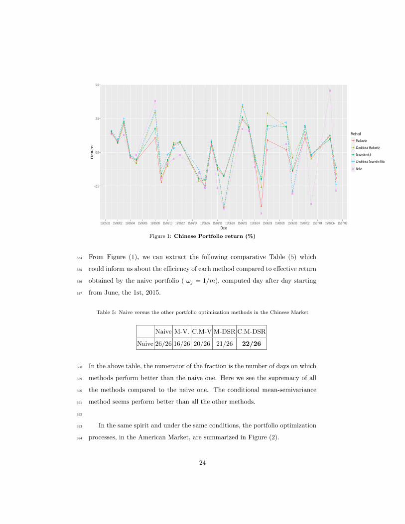
For the Chinese Market, results are summarized in the Figure (1). It is clear379
that, in term of returns, all the portfolios obtained from the optimization meth-380
ods are dominating the naive one. The conditional methods perform better than381
the non conditional ones.382
383
23
●
●
●
●●
●
●
●
●
●
●
●
●
●
●
●
●
●
●
●
●
●
●
●
●
●
−2.5
0.0
2.5
5.0
15/05/31 15/06/02 15/06/04 15/06/06 15/06/08 15/06/10 15/06/12 15/06/14 15/06/16 15/06/18 15/06/20 15/06/22 15/06/24 15/06/26 15/06/28 15/06/30 15/07/02 15/07/04 15/07/06 15/07/08Date
Re
turn
Method● Markowitz
Conditional Markowitz
Downside risk
Conditional Downside Risk
Naive
Figure 1: Chinese Portfolio return (%)
From Figure (1), we can extract the following comparative Table (5) which384
could inform us about the efficiency of each method compared to effective return385
obtained by the naive portfolio ( ωj = 1/m), computed day after day starting386
from June, the 1st, 2015.387
Table 5: Naive versus the other portfolio optimization methods in the Chinese Market
Naive M-V. C.M-V M-DSR C.M-DSR
Naive 26/26 16/26 20/26 21/26 22/26
In the above table, the numerator of the fraction is the number of days on which388
methods perform better than the naive one. Here we see the supremacy of all389
the methods compared to the naive one. The conditional mean-semivariance390
method seems perform better than all the other methods.391
392
In the same spirit and under the same conditions, the portfolio optimization393
processes, in the American Market, are summarized in Figure (2).394
24
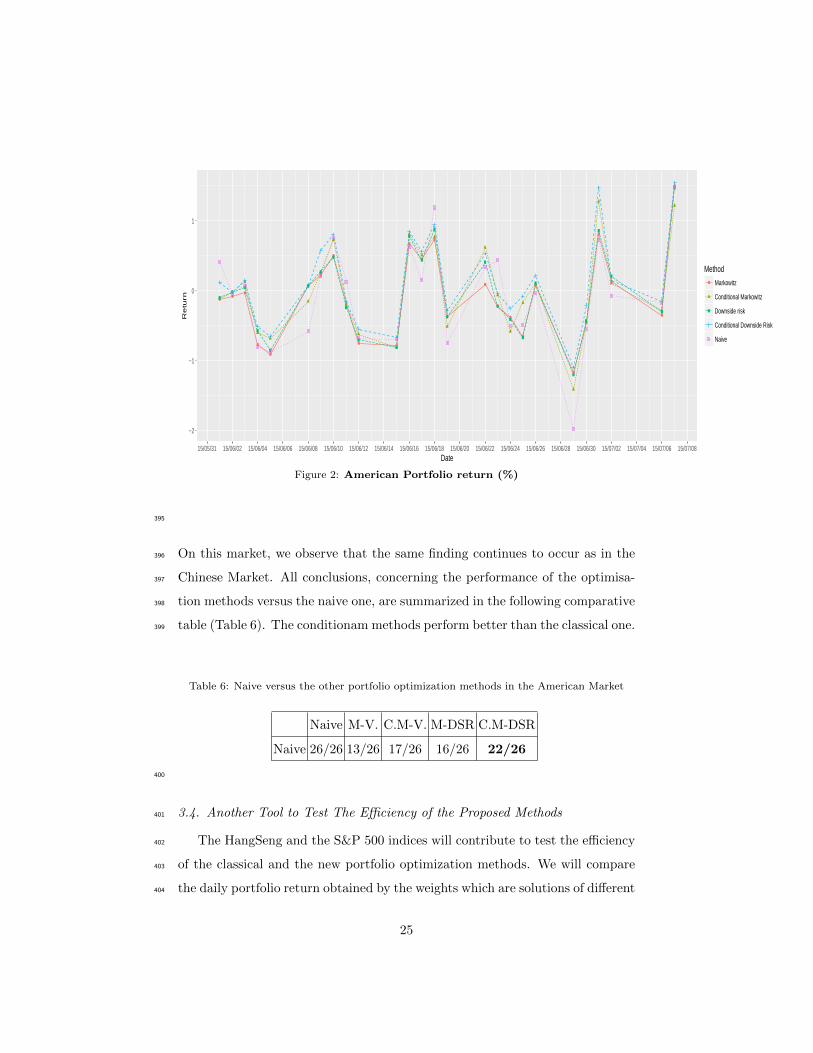
●●
●
●
●
●
●
●
●
● ●
●
●
●
●
●
●
●
●
●
●
●
●
●
●
●
−2
−1
0
1
15/05/31 15/06/02 15/06/04 15/06/06 15/06/08 15/06/10 15/06/12 15/06/14 15/06/16 15/06/18 15/06/20 15/06/22 15/06/24 15/06/26 15/06/28 15/06/30 15/07/02 15/07/04 15/07/06 15/07/08Date
Re
turn
Method● Markowitz
Conditional Markowitz
Downside risk
Conditional Downside Risk
Naive
Figure 2: American Portfolio return (%)
395
On this market, we observe that the same finding continues to occur as in the396
Chinese Market. All conclusions, concerning the performance of the optimisa-397
tion methods versus the naive one, are summarized in the following comparative398
table (Table 6). The conditionam methods perform better than the classical one.399
Table 6: Naive versus the other portfolio optimization methods in the American Market
Naive M-V. C.M-V. M-DSR C.M-DSR
Naive 26/26 13/26 17/26 16/26 22/26
400
3.4. Another Tool to Test The Efficiency of the Proposed Methods401
The HangSeng and the S&P 500 indices will contribute to test the efficiency402
of the classical and the new portfolio optimization methods. We will compare403
the daily portfolio return obtained by the weights which are solutions of different404
25
optimization programs using all the data until May the 31th , 2015. From June405
the 1st, 2015 until July the 7th, 2015, we compute the portfolio returns and we406
compare them against the daily HangSeng and the S&P 500 indices. Results407
are exhibited in figure 4.1 (the Chinese Market) and figure 4.2 (the American408
Market).409
• Red color signifies a negative difference between portfolio return and HangSeng410
Index (respectively S&P 500 index).411
• Blue color signifies a positive difference between portfolio return and HangSeng412
Index (respectively S&P 500 index).413
• Overall performance is the sum of all the differences during the test period.414
We note that the comparison is in favour of the Conditional-Mean-Variance and415
the Conditional-Mean-Semivariance optimization methods. The overall perfor-416
mance varies depending on the method of portfolio optimization and markets:417
• From 0.94% (Classical Markowitz method) to 12.64% (Conditional Mean-418
Semivariance method) for the the Chinese Market,419
• From 0.09% (Classical Markowitz method) to 1.42% (Conditional Mean-420
Semivariance method) for the American Market.421
These mouthwatering results deserve more practice and more tests over a long422
period of time and on different markets using different financial products.423
424
26
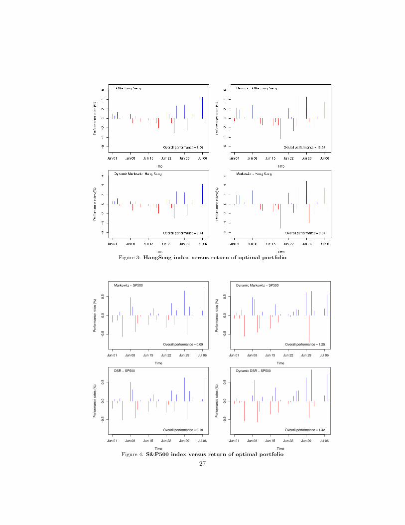
Figure 3: HangSeng index versus return of optimal portfolio
Jun 01 Jun 08 Jun 15 Jun 22 Jun 29 Jul 06
−0.5
0.0
0.5
Time
Perf
orm
ance r
ate
s (
%)
Markowitz − SP500
Overall performance = 0.09
Jun 01 Jun 08 Jun 15 Jun 22 Jun 29 Jul 06
−0.5
0.0
0.5
Time
Perf
orm
ance r
ate
s (
%)
Dynamic Markowitz − SP500
Overall performance = 1.25
Jun 01 Jun 08 Jun 15 Jun 22 Jun 29 Jul 06
−0.5
0.0
0.5
Time
Perf
orm
ance r
ate
s (
%)
DSR − SP500
Overall performance = 0.19
Jun 01 Jun 08 Jun 15 Jun 22 Jun 29 Jul 06
−0.5
0.0
0.5
Time
Perf
orm
ance r
ate
s (
%)
Dynamic DSR − SP500
Overall performance = 1.42
Figure 4: S&P500 index versus return of optimal portfolio
27

4. Conclusion425
In this paper, we developed two new approaches in order to get an optimal426
portfolio minimizing two conditional risks.427
• The first risk is based on conditional variance. In this case, the optimiza-428
tion method is an extension of the classical Mean-Variance model. What429
we proposed is to replacing Mean and Variance by Conditional Mean and430
Conditional Variance estimators.431
• The second one is based on Conditional Semivariance. In this case, the432
optimization method is an extension of the classical Mean-Semivariance433
model. What we proposed is to replacing Mean and Semivariance by434
Conditional Mean and Conditional semivariance estimators.435
This novelty, using conditional risk, gives a new approach and a more efficient436
alternative to get an optimal portfolio. In fact, all the other methods do not437
anticipate the future and just extrapolate to the future what we observed in the438
past.439
In both cases, the optimization algorithm involved using the Lagrangian440
method. Even, our results seem interesting, the efficiency of our methods should441
be confirmed on other markets and with other various assets. Kernel methods,442
belonging to nonparametric methods, are used to estimate Conditional Mean,443
Variance and Semivariance. Product Gaussian densities are used as kernel.444
It will be very helpful to choose typical multivariate kernels. Similarly, we445
should develop a global method to choose the bandwidth which is crucial in446
nonparametic estimation.447
Back to results of this paper: the Conditional Mean-Semivariance seem most448
appropriate to get an optimal portfolio using the data of the Chinese and the449
American markets. By the way, Conditional Mean-Variance is more efficient450
than Mean-Variance method. Similarly, the Conditional Mean-Semivariance is451
better than the Mean-Semivariance method.452
28
Thanks to its robustness, it is also reasonable to substitute the conditional453
median to the conditional mean and to propose an optimization model based454
on Conditional Median and conditional variance or conditional Median and455
Conditional Semivariance. This topic will be treated as a matter for future456
research.457
References458
H. Markowitz, Portfolio Selection, Journal of Finance 7 (1952) 77–-91.459
H. Markowitz, Portfolio Selection : Efficient Diversification of Investments,460
1959.461
H. Markowitz, Mean-Variance Analysis in Portfolio Choice and Capital Markets,462
Basil Blackwell, 1990.463
R. O. Michaud, The Markowitz Optimization Enigma: Is ‘Optimized’ Optimal?,464
Financial Analysts Journal 45 (1989) 31–42.465
F. Black, R. Litterman, Global portfolio optimization, Financial Analysts Jour-466
nal 48 (5) (1992) 28–43.467
A. F. Siegel, A. Woodgate, Performance of Portfolios Optimized with Estimation468
Error, Management Science 53 (6) (2007) 1005–15.469
O. Ledoit, M. Wolf, Honey, I Shrunk the Sample Covariance Matrix, The Journal470
of Portfolio Management 30 (4) (2004) 110–9.471
M. Levy, R. Roll, The Market Portfolio May Be Mean/Variance Efficient After472
All, Review of Financial Studies, 23 (6) (2010) 2464–91.473
E.-I. Delatola, J. E. Griffin, Bayesian Nonparametric Modelling of the Return474
Distribution with Stochastic Volatility, Bayesian Analysis 6 (4) (2011) 901–26.475
A. Kresta, Application of GARCH-Copula Model in Portfolio Optimization,476
Financial Assets and Investment (2) (2015) 7–20.477
29
J. Tobin, Estimation of Relationships for Limited Dependent Variables, Econo-478
metrica 26 (1) (1958) 24–36.479
F. D. Arditti, Another Look at Mutual Fund Performance, Journal of Financial480
and Quantitative Analysis 6 (3) (1971) 909–12.481
P. Chunhachinda, K. Dandapani, S. Hamid, A. Prakash, Portfolio Selection and482
Skewness: Evidence from International Stock Markets, Journal of Banking483
and Finance 21 (1997) 143–67.484
A. Prakash, C. Chang, T. Pactwa, Selecting a Portfolio with Skewness: Recent485
Evidence from US, European, and Latin American Equity Markets, Journal486
of Banking and Finance 27 (2003) 1375–90.487
J. Estrada, Mean-Semivariance Behavior : An Alternative Behavioural Model,488
Journal of Emerging Market Finance 3 (2004) 231–48.489
J. Estrada, Optimization : A Heuristic Approach, Journal of Applied Finance490
(2008) 57–72.491
W. Hogan, J. Warren, Computation of the efficient Boundary in the ES Portfolio492
selection, Journal of Financial and Quantitative Analysis 9 (1974) 1–11.493
J. S. Ang, A Note on the ESL Portfolio Selection Model, The Journal of Finan-494
cial and Quantitative Analysis 10 (5) (1975) 849–57.495
V. Harlow, Asset allocation in a downside risk framework, Financial Analyst496
Journal 47 (1991) 28–40.497
C. Mamoghli, S. Daboussi, Optimisation de portefeuille downside risk, Social498
Science Research Network 23.499
H. Markowitz, P. Todd, G. Xu, Y. Yamane, Computation of mean-Semivariance500
efficient sets by the critical line algorithm, Annals of Operations Research 45501
(1993) 307–17.502
30
G. Athayde, Building a Mean-Downside Risk Portfolio Frontier, Developments503
in Forecast Combination and Portfolio Choice, 2001.504
G. Athayde, The mean-downside risk portfolio frontier : a non-parametric The505
mean-downside risk portfolio frontier : a non-parametric approach, Advances506
in portfolio construction and implementation, 2003.507
H. Ben Salah, M. Chaouch, A. Gannoun, C. de Peretti, A. Trabelsi, Median-508
based Nonparametric Estimation of Returns in Mean-Downside Risk Port-509
folio frontier, Annals of Operations Research doi:10.1007/s10479-016-2235-z510
(2016a) 1–29.511
H. Ben Salah, A. Gannoun, C. de Peretti, M. Ribatet, A. Trabelsi, A New512
Approach in Nonparametric Estimation of Returns in Mean-Downside Risk513
Portfolio frontier, submitted (2016) .514
D. Bosq, J.-P. Lecoutre, Theorie de l’Estimation Fonctionnelle, Economica,515
1987.516
L. Wasserman, All of nonparametric statistics, Springer, 2006.517
P. Sarda, Smoothing parameter selection for smooth distribution functions,518
Journal of Statistical Planning and Inference 35 (1993) 65–75.519
N. Altman, C. Leger, Bandwidth Selection for Kernel Distribution Function520
Estimation, Journal of Statistical Planning and Inference 46 (1995) 195–214.521
Y. Li, M. Hong, N. Tuner, J. Lupton, R. Caroll, estimation of correlation func-522
tions in longitudinal and spatial data, with application to colon carcinogenesis523
experiments, Ann. Statist 35 (2007) 1608–43.524
D. Vasant, M. Jarke, J. Laartz, Big Data, Business & Information Systems525
Engineering 6 (5) (2014) 257–9.526
S. Arlot, A. Celisse, A survey of cross-validation procedures for model selection,527
Statistics Surveys (4) (2010) 40–79.528
31