University of Illinois at Urbana-Champaign

Air Conditioning and Refrigeration Center A National Science Foundation/University Cooperative Research Center

Condensing Units for Household Refrigerator-Freezers

T. Kulkarni, M.-H. Kim, and C. W. Bullard

ACRC CR-38 June 2001

For additional information: Air Conditioning and Refrigeration Center University of Illinois Mechanical & Industrial Engineering Dept. 1206 West Green Street Urbana, IL 61801 (217) 333-3115

The Air Conditioning and Refrigeration Center was founded in 1988 with a grant from the estate of Richard W. Kritzer, the founder of Peerless of America Inc. A State of Illinois Technology Challenge Grant helped build the laboratory facilities. The ACRC receives continuing support from the Richard W. Kritzer Endowment and the National Science Foundation. The following organizations have also become sponsors of the Center. Amana Refrigeration, Inc. Arçelik A. S. Brazeway, Inc. Carrier Corporation Copeland Corporation Dacor Daikin Industries, Ltd. DaimlerChrysler Corporation Delphi Harrison Thermal Systems Frigidaire Company General Electric Company General Motors Corporation Hill PHOENIX Honeywell, Inc. Hussmann Corporation Hydro Aluminum Adrian, Inc. Indiana Tube Corporation Invensys Climate Controls Kelon Electrical Holdings Co., Ltd. Lennox International, Inc. LG Electronics, Inc. Modine Manufacturing Co. Parker Hannifin Corporation Peerless of America, Inc. Samsung Electronics Co., Ltd. Tecumseh Products Company The Trane Company Thermo King Corporation Valeo, Inc. Visteon Automotive Systems Wolverine Tube, Inc. York International, Inc. For additional information: Air Conditioning & Refrigeration Center Mechanical & Industrial Engineering Dept. University of Illinois 1206 West Green Street Urbana, IL 61801 217 333 3115

iii

Table of Contents

Page

List of Figures ............................................................................................................................ iv

List of Tables ............................................................................................................................... v

I. Introduction.............................................................................................................................. 1

II. Compressor Analysis ........................................................................................................... 2

1. Introduction ............................................................................................................................2

2. Simple compressor model ......................................................................................................3

3. Simulation and parameter estimation results .........................................................................6

4. Conclusions.......................................................................................................................... 11

III. Sub-Condenser Design.....................................................................................................12

1. Condenser Simulation Models.............................................................................................. 12

1.1 Introduction...............................................................................................................................................................12

1.2 Condenser geometry ...............................................................................................................................................12

1.3 Simulation models ..................................................................................................................................................15

1.4 Air-side pressure drop assumptions.....................................................................................................................24

1.5 Condenser performance in actual refrigerator....................................................................................................26

2. Optimization of sawtooth condenser .................................................................................... 26

2.1 Simulation of wind tunnel experiments................................................................................................................26

2.2 Simulation of compressor-condenser subsystem................................................................................................27

2.3 Optimization of sawtooth geometry......................................................................................................................29

2.4 Effect of constant fan power..................................................................................................................................31

2.5 Optimization of sawtooth condenser in cross-counterflow arrangement .......................................................32

2.6 Discussion of results ................................................................................................................................................33

References.................................................................................................................................37

Appendix A. Data sets used for the model and simulation results ............................39

Appendix B. Uncertainty of wind tunnel tests .................................................................41

iv

List of Figures

Page

Part II Compressor Analysis

Fig. 1 Schematic diagram of a reciprocating compressor..........................................................................................................4 Fig. 2 Specific volumes as function of suction pressure...........................................................................................................8 Fig. 3 Volumetric efficiency..........................................................................................................................................................9 Fig. 4 Refrigerant mass flow rate..................................................................................................................................................9 Fig. 5 Compressor efficiency as a function of discharge temperature....................................................................................9 Fig. 6 Power consumption............................................................................................................................................................10 Fig. 7 Compressor shell temperature as a function of discharge temperature ......................................................................10 Fig. 8 Discharge temperature .......................................................................................................................................................11

Part III Sub-Condenser Design

Fig. 1.1 Duct geometry .................................................................................................................................................................14 Fig. 1.2 Vertical Cross-counterflow coil and Air Flow...........................................................................................................15 Fig. 1.3 Sawtooth condenser configuration and airflow arrangement ...................................................................................23 Fig. 2.1 Refrigeration Cycle on P-h diagram............................................................................................................................28 Fig. 2.2 COP vs Te at constant Tcond (polynomial fit) ..........................................................................................................34 Fig. 2.3 COP vs. Te at constant Tcond (Kim and Bullard [3]) ..............................................................................................35

v

List of Tables

Page

Part II Compressor Analysis

Table 1. Data sets used for computer simulations......................................................................................................................6 Table 2. Estimated parameters ......................................................................................................................................................7 Table 3. RMS errors ........................................................................................................................................................................7 Table 1.1 Specifications of condensers .......................................................................................................................................13 Table 1.2 Test conditions.............................................................................................................................................................19 Table 1.3 Vertical cross-counterflow simulation Results(C/F#1) .........................................................................................19 Table 1.4 Vertical cross-counterflow simulation results(C/F#2) ..........................................................................................20 Table 1.5 Vertical cross-counterflow simulation results(C/F#3) ..........................................................................................20 Table 1.6 Spiral condenser simulation results (spiral#1) ........................................................................................................21 Table 1.7 Spiral condenser simulation results (spiral#2) ........................................................................................................22 Table 1.8 Spiral condenser simulation results (spiral#3) .........................................................................................................22 Table 1.9 Sawtooth condenser simulation results (S/T#1) ......................................................................................................24 Table 1.10 Sawtooth condenser simulation results (S/T#2) ....................................................................................................24 Table 1.11 Additional pressure drop...........................................................................................................................................25 Table 1.12 Machine room experimental results ........................................................................................................................26

Part III Sub-Condenser Design

Table 2.1 Prototype condenser simulation .................................................................................................................................28 Table 2.2 Constraints on optimization ........................................................................................................................................30 Table 2.3 Results of optimization (constant fan efficiency)....................................................................................................31 Table 2.3a Results of optimization (constant fan power) ........................................................................................................32 Table 2.4 Optimization of cross-counterflow sawtooth condenser........................................................................................33

Appendix A

A1 Data set I ....................................................................................................................................................................................39 A2 Data set II ...................................................................................................................................................................................39 A3 Data set III .................................................................................................................................................................................40

Appendix B

Table B1 Uncertainty in measured air-side capacity (C/F#1) .................................................................................................41 Table B2 Uncertainty in measured air-side capacity (Spiral#1) .............................................................................................41 Table B3 Uncertainty in measured air-side capacity (S/T#1).................................................................................................42

1

I. Introduction

Refrigerator-freezer is a major household appliance designed for preserving foods through refrigerating and

freezing. The increasing market demand for energy saving of the household appliance speed up to develop energy

efficient system. The energy use of U.S. refrigerators has declined more than 60% in the last 25 years but changes in

U.S. refrigerator minimum efficiency standards are reducing refrigerator energy use by around 25% below current

levels [1]. To improve thermal efficiency of the system, the performance of the components constituting the

refrigeration system should all be improved simultaneously. Reduction of thermal resistance of both condenser and

evaporator is necessary in addition to higher compressor efficiency, improved characteristics of the expansion

device, and better insulation of the enclosure. As a first step toward the eventual goal, the research project is focused

on the condensing unit, which is composed of a compressor, a sub-condenser and a cooling fan.

The optimum arrangement of the condensing unit as well as the configuration of the sub-condenser is

important to improve energy efficiency of the system, and reduce installation space and eventually increase

available volume of refrigerator or freezer compartment. Improving thermal performance of the sub-condenser is

required to reduce thermal resistance between refrigerant and environment. According to the previous research on

wire-on-tube condensers, the external resistance for a refrigerator condenser is at least 95% of the total thermal

resistance for the two-phase region and greater than 62% for the superheated and sub-cooled regions [2]. Therefore,

decreasing the air-side thermal resistance is needed. To reduce this resistance, the surface area of the sub-condenser

can be increased or the air-side heat transfer coefficient can be improved. However, the overall size of the sub-

condenser is somewhat limited by economic and spatial constraints. Therefore, this project concentrated primarily

on optimizing the air-side configuration of the sub-condenser.

In addition, reasonable performance data of the compressor with given operation condition is needed for

system designer to make optimal design of the system. Compressor manufacturers usually provide empirical

performance curves called compressor maps, expressing mass flow and power input as polynomial functions of

evaporation temperature for a range of condensing temperatures. Since they are based on fixed ambient and suction

gas temperatures, the maps are useful for comparing and selecting the compressors. However, they are inadequate

for general system analysis, because they contain no information about the effects of different ambient and suction

temperatures and are unable to predict discharge temperatures, which define the condenser inlet condition. There are

several detailed compressor models in the open literature, but they usually require large sets of unknown parameters

to characterize the complicated refrigerant flow, heat exchanges, effects of oil, moving boundaries, and data on the

geometry and heat transfer characteristics of internal parts. Most such models contain too little data to distinguish

accurate parameter estimation from merely "tuning" the model for a few selected operating conditions. The research

project is focusing on this issue in order to establish a foundation for the development of a simple physical model of

small hermetic reciprocating compressors, suitable for use in the design of refrigerator-freezers. Unlike the

polynomial functions in compressor maps, it may be safer to extrapolate physically-based models outside the range

of compressor calorimeter operating capabilities.

2

II. Compressor Analysis

The basic purpose of the compressor sub-model in a larger system model is to provide the refrigerant mass

flow rate, power consumption and discharge states of the compressor using some given information. The usual input

data are compressor geometry (displacement and clearance volume), compressor speed, suction pressure and

temperature, discharge pressure, and ambient temperature.

A mass flow rate model reflects clearance volumetric efficiency and simulates suction gas heating using an

empirical relationship: the specific volume at the suction port of the cylinder has linear relationship with the specific

volume at the compressor suction. Compressor work is calculated using the compressor efficiency represented by

some empirical parameters. A linear relationship between the discharge and shell temperatures will be used for

calculating the discharge temperature.

The goal is to develop a general but simple model for reciprocating compressors for refrigerator-freezers

using R-134a refrigerant, to provide reasonable compressor performance data to system designer. The basic simple

physical model [3] was developed based on thermodynamic principles and large data sets from compressor

calorimeter and in-situ tests [4, 5].

1. Introduction The compressor is one of major components of an air conditioning or refrigeration system and has an

important effect on system energy efficiency. Compressor manufacturers usually provide empirical performance

curves called compressor maps, expressing mass flow and power input as polynomial functions of evaporation

temperature for a range of condensing temperatures. Since they are based on fixed ambient and suction gas

temperatures, the maps are useful for comparing and selecting the compressors. However, they are inadequate for

general system analysis, because they contain no information about the effects of different ambient and suction

temperatures and are unable to predict discharge temperatures, which define the condenser inlet condition. Dabiri

and Rice [6] suggested additional assumptions to account for suction gas heating, which have been used with limited

success for reciprocating compressors with low-side sumps, and with greater success for rotary compressors where

the suction gas is injected directly [7]. Haider et al. [8] investigated the effect of compressor map and ambient

temperature on the power consumption of a refrigerator-freezer using the ERA (EPA Refrigerator Analysis)

software, complemented by the measured compressor and refrigerator-freezer data. They reported the accuracy of

ERA estimation could be improved up to 5.1% at an ambient temperature of 43.3oC by using the measured map data

at 43.3oC rather than the given map at standard test condition of 32.2oC.

There are several detailed physical models of compressors in the literature. Prakash and Singh [9]

developed a mathematical model for a reciprocating compressor using the first law of thermodynamics and

assuming the refrigerant is an ideal gas. Hiller and Glicksmann [10] reported a detailed compressor model of

reciprocating compressors and compared the simulation results with experimental data. Domanski and Didion [11]

developed a quite detailed compressor model for a system simulation, but it requires over 30 input parameters.

Todescat et al. [12] presented a thermal energy analysis of a reciprocating hermetic compressor using the energy

balances for several parts of the compressor. They reported the effect of compressor shell temperature on the

compressor performance such as power consumption and energy efficiency ratio. Recently, Cavallini et al. [13]

3

presented a steady state model for the thermal analysis of an hermetic reciprocating compressor and compared with

a few experimental data points for R-134a and R-600a compressors. Rigola et al. [14] presented an advanced

numerical scheme of the thermal and fluid dynamic behavior of small hermetic reciprocating compressors, along

with some empirical data. Those models usually require large sets of unknown parameters to characterize the

complicated refrigerant flow, heat exchanges, effects of oil, and moving boundaries, plus data on the geometry and

heat transfer characteristics of internal parts. Most such papers contain too little data to distinguish accurate

parameter estimation from merely "tuning" the model for a few selected operating conditions. Klein and Reindl [15]

developed a model similar to that presented here, which embodies different physical assumptions underlying the

mass flow and power submodels.

The purpose of this study is to extend to different type of reciprocating compressors on approach explored

first for small hermetic reciprocating compressors [3] and provide the reasonable compressor data to system

designer. Instead of taking a detailed approach, the goal is to find the simplest formulation suitable for use in

refrigerator model. Pressure losses along the refrigerant path are neglected and the compression process is assumed

as isentropic. A mass flow rate model reflects clearance volumetric efficiency and simulates suction gas heating

using an empirical relationship: the specific volume at the suction port of the cylinder has linear relationship with

the specific volume at the compressor suction. Compressor work is calculated using the compressor efficiency

represented by only two empirical parameters. A linear relationship between the discharge and shell temperatures is

extracted from the data and used for calculating the discharge temperature for any ambient air temperature.

2. Simple compressor model The basic purpose of the compressor sub-model in a larger system model is to provide the refrigerant mass

flow rate, power consumption and discharge states of the compressor using some given information. The usual input

data are compressor geometry (displacement and clearance volume), compressor speed, suction pressure and

temperature, discharge pressure, and ambient temperature.

A detailed thermodynamic model of a compressor is extremely complex due to the inherently complicated

structure of the compressor and refrigerant flow pathways, along which heat transfer and pressure vary substantially

and rapidly. For some applications (e.g. design of variable-speed drives) such detailed modeling is necessary [16].

Our hypothesis is that the requirements for quasi-steady system simulation modeling are much less demanding, so

several assumptions can be made to simplify the physical model for small hermetic reciprocating compressors:

1. The refrigerant path can be treated as a steady state flow; 2. The compression process is isentropic; 3. The kinetic and potential energies of refrigerant are neglected; 4. The pressure losses along the refrigerant path are neglected; 5. The oil effects on the refrigerant properties are neglected.

4

Suction (Psuc, Tsuc)

Discharge (Pdis, Tdis)

Discharge port (Pdp, Tdp)

Suction muffler

Suction port (Psp, Tsp)

Shell

Electric motor

Cylinder

Fig. 1 Schematic diagram of a reciprocating compressor

Fig. 1 shows a schematic diagram for typical low-side sump reciprocating compressor. The following is a

simple description for the refrigerant compression process of a low-side sump reciprocating compressor. Refrigerant

vapor at low pressure and temperature enters the compressor shell through suction line and is heated as it cools the

motor and other parts, and mixes with hot plenum gas along the refrigerant suction path. After compression in the

cylinder, high temperature and pressure refrigerant gas discharges through a muffler, rejecting heat to the plenum

gas before exiting via the discharge line. Therefore, for the low-side sump compressors most of the shell is at low

suction pressure.

For a given compressor velocity and swept volume, the mass flow rate can be calculated using the

volumetric efficiency [17].

sp

dispv

v

Vm

ωη60=& (2.1)

The volumetric efficiency for reciprocating compressors is given by Eq. (2.2), which accounts for re-

expansion of the gas remaining in the clearance volume.

−−= 1

),(1

spdp

spv sPv

vCη (2.2)

For a small hermetic compressor, we assume compression and re-expansion processes to be isentropic so

the specific volume at the discharge port of the cylinder can be calculated. The decrease in density due to suction gas

heating and mixing between the suction line to suction port has a large effect on the volumetric efficiency and mass

flow rate.

5

For small hermetic reciprocating compressors considered here, the following empirical relations are

obtained using least squares from the mass flows and suction pressure (Fig. 3)

sucsp

sucsuc

Pc

cv

Pc

cv

43

21

+=

+= (2.3)

where c1, c2, c3, and c4 are constants to be determined.

Rearranging the Eq. (2.3) shows relationship between the specific volume for the suction and suction port

sucsp vaav 21 += (2.4)

where the constants can be estimated directly from the same experimental data.

The constants of Eqs. (2.3) and (2.4) are determined by minimizing the following objective function to

obtain the best agreement with the measured mass flow rate at N data points.

N

m

mm

mobj

N

n

cal∑=

−

=1

2

exp

exp

min_&

&&

& (2.5)

The compressor power consumption can be calculated if the compressor efficiency is known. The

isentropic compressor efficiency is normally defined across the entire compressor shell, but in our case we define a

compression efficiency that excludes the effects of subsystem heat transfers upstream of the suction port, and

includes the effects of motor efficiency:

WhsPhm spspdpc /]),([ −= &η (2.6)

Empirical observation (Fig. 5) shows that the compressor efficiency can be expressed simply as:

disc Tkk 21 +=η (2.7)

where the constants k1 and k2 can be estimated by minimizing the average normalized deviation between measured

and calculated power consumption

N

W

WW

Wobj

N

n

cal∑=

−

=1

2

exp

exp

min_ (2.8)

The empirically observed dependence of compression efficiency on shell temperature is thought to reflect

the temperature dependence of oil viscosity. The principal mechanism of oil cooling, splattering into the compressor

shell, determines the relationship between shell temperature and oil temperature.

6

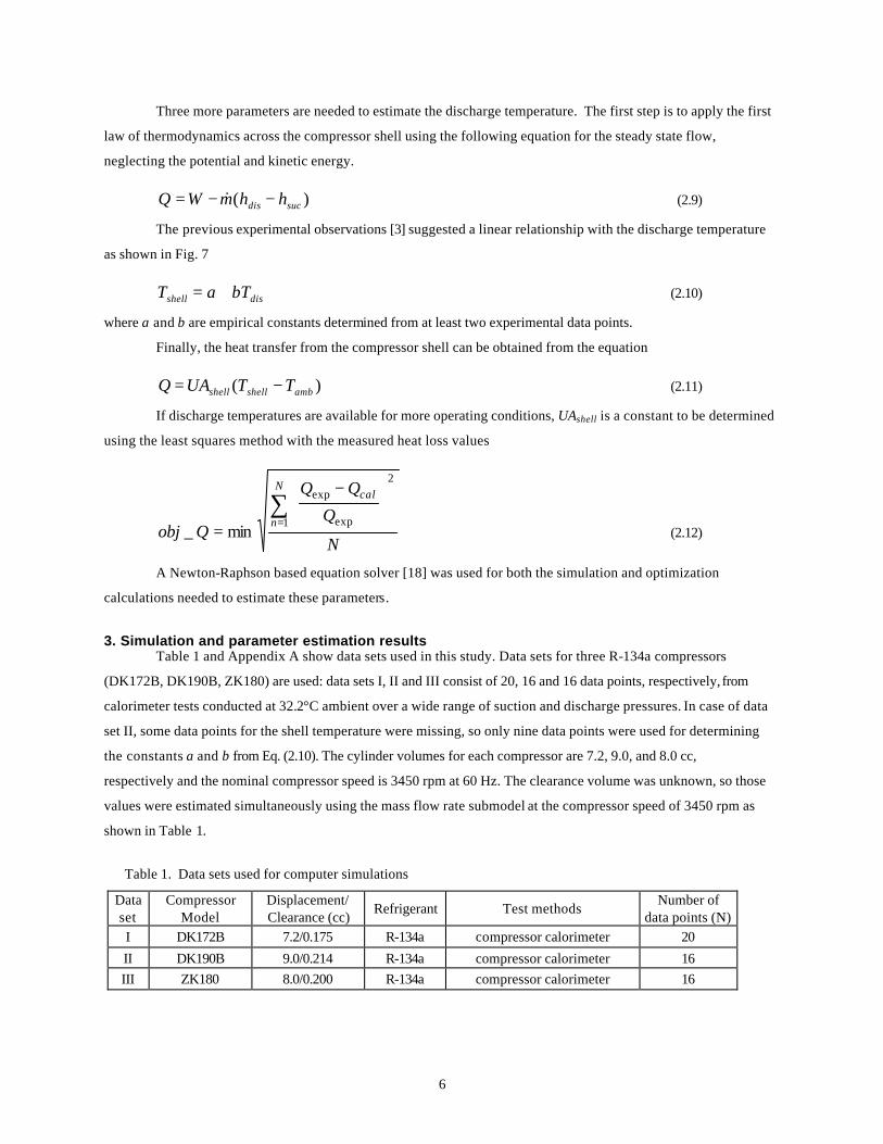
Three more parameters are needed to estimate the discharge temperature. The first step is to apply the first

law of thermodynamics across the compressor shell using the following equation for the steady state flow,

neglecting the potential and kinetic energy.

)( sucdis hhmWQ −−= & (2.9)

The previous experimental observations [3] suggested a linear relationship with the discharge temperature

as shown in Fig. 7

disshell bTaT += (2.10)

where a and b are empirical constants determined from at least two experimental data points.

Finally, the heat transfer from the compressor shell can be obtained from the equation

)( ambshellshell TTUAQ −= (2.11)

If discharge temperatures are available for more operating conditions, UAshell is a constant to be determined

using the least squares method with the measured heat loss values

N

Q

QQ

Qobj

N

n

cal∑=

−

=1

2

exp

exp

min_ (2.12)

A Newton-Raphson based equation solver [18] was used for both the simulation and optimization

calculations needed to estimate these parameters.

3. Simulation and parameter estimation results Table 1 and Appendix A show data sets used in this study. Data sets for three R-134a compressors

(DK172B, DK190B, ZK180) are used: data sets I, II and III consist of 20, 16 and 16 data points, respectively, from

calorimeter tests conducted at 32.2°C ambient over a wide range of suction and discharge pressures. In case of data

set II, some data points for the shell temperature were missing, so only nine data points were used for determining

the constants a and b from Eq. (2.10). The cylinder volumes for each compressor are 7.2, 9.0, and 8.0 cc,

respectively and the nominal compressor speed is 3450 rpm at 60 Hz. The clearance volume was unknown, so those

values were estimated simultaneously using the mass flow rate submodel at the compressor speed of 3450 rpm as

shown in Table 1.

Table 1. Data sets used for computer simulations

Data set

Compressor Model

Displacement/ Clearance (cc)

Refrigerant Test methods Number of

data points (N) I DK172B 7.2/0.175 R-134a compressor calorimeter 20

II DK190B 9.0/0.214 R-134a compressor calorimeter 16 III ZK180 8.0/0.200 R-134a compressor calorimeter 16

7

The simulation results are depicted in Figs. 3–8, compared with measured values. Tables 2 and 3 show the

estimated parameters and RMS errors of simulation results for each data set, respectively. The parameter estimates

were obtained using the complete data sets , except missing data; the small standard deviations apparent from Figs.

3-8 indicate that smaller subsets of data could yield similar results. The overall calculation results are in good

agreement with measured data within a reasonable accuracy (especially considering measurement accuracy) as

shown in Table 3: the RMS errors for calculated mass flow rates and power inputs are within 2.5% and 2.9%, and

the difference between the calculated and measured discharge temperatures is below 3.8oC.

Table 2. Estimated parameters

Estimated constants Data set

c3 c4 k1 k2 a b UAshell

I -0.03135 31.85 0.367 0.00289 43.77 0.255 3.69

II -0.00483 27.23 0.255 0.00343 26.27 0.474 3.65

III -0.00652 26.65 0.315 0.00336 46.48 0.248 3.57

Table 3. RMS errors

RMS errors

% oC Data set

obj_mr obj_W ∆Tdis

I 2.50 0.52 3.5

II 1.47 2.85 3.8

III 1.48 2.10 3.7

Figs. 2-4 present the simulation results of the mass flow rate submodel. Fig. 2 shows the linear

relationships between the specific volumes at the suction and suction ports and the inverse of suction pressure. The

specific volumes at the suction port are consistently larger than those at the suction, suggesting that the suction gas

is heated as it cools the motor and other parts and mixes with hot plenum gas along the refrigerant suction path. The

suction gas heating and mixing cause density decrease, which is a very important factor affecting mass flow rate.

Fig. 3 presents the clearance volumetric efficiency. As expected, the volumetric efficiency decreases systematically

with the pressure ratio. It varies from 0.9 to 0.6 with increasing pressure ratio of 5 to 20, and has a value of about

0.83 at the normal operating condition where the pressure ratio is around 10. Fig. 4 presents a comparison of the

calculated and measured mass flow rates and they are in excellent agreement over a whole range of test conditions.

8

0.006 0.008 0.01 0.012 0.014 0.016 0.1

0.2

0.3

0.4

0.5

1 / P s u c ( 1 / k P a )

v s p

v s u c

v s u c ,

v s p

( m 3 / k

g )

(a) DK172B

0.006 0.008 0.01 0.012 0.014 0.016 0.1

0.2

0.3

0.4

0.5

1 / P s u c ( 1 / k P a )

v s u c ,

v s p ( m

3 / k

g )

v s p

v s u c

(b) DK190B

0.006 0.008 0.01 0.012 0.014 0.016 0.1

0.2

0.3

0.4

0.5

1 / P s p ( k P a - 1

)

v s u c

,

v s p

[ m 3 / k

g ]

v s u c

v s p

(c) ZK180

Fig. 2 Specific volumes as function of suction pressure

9

5 10 15 20 25 0.5

0.6

0.7

0.8

0.9

1

P d p / P

s p

DK172B DK190B ZK180

? v

Fig. 3 Volumetric efficiency

0 1 2 3 4 5 6 7 8 9 10 0

2

4

6

8

10

m e x p ( k g / h )

m c a

l ( k g

/ h )

DK190B DK172B

ZK180

Fig. 4 Refrigerant mass flow rate

50 60 70 80 90 100 110 0.4

0.5

0.6

0.7

0.8

0.9

T d i s (

o C )

DK190B DK172B

ZK180

?c

Fig. 5 Compressor efficiency as a function of discharge temperature

10

50 100 150 200 250 300 50

100

150

200

250

300

W e x p ( W )

W c a

l ( W )

DK190B DK172B

ZK180

Fig. 6 Power consumption

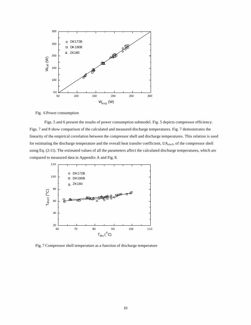
Figs. 5 and 6 present the results of power consumption submodel. Fig. 5 depicts compressor efficiency.

Figs. 7 and 8 show comparison of the calculated and measured discharge temperatures. Fig. 7 demonstrates the

linearity of the empirical correlation between the compressor shell and discharge temperatures. This relation is used

for estimating the discharge temperature and the overall heat transfer coefficient, UAshell, of the compressor shell

using Eq. (2-11). The estimated values of all the parameters affect the calculated discharge temperatures, which are

compared to measured data in Appendix A and Fig. 8.

60 70 80 90 100 110 20

40

60

80

100

120

T d i s ( o C )

T s h

e l l ( o

C )

DK190B DK172B

ZK180

Fig. 7 Compressor shell temperature as a function of discharge temperature

11

50 60 70 80 90 100 110 120 50

60

70

80

90

100

110

120

T d i s , e x p ( o C )

T d i s

, c a l (

o C )

DK190B DK172B

ZK180

Fig. 8 Discharge temperature

4. Conclusions A simple and general compressor model developed using the thermodynamic principles and large data sets

from the compressor calorimeter and in-situ tests has been successfully applied to the different type of reciprocating

compressors. The model can estimate mass flow rate and compressor power consumption with rms errors less than

3.0%, which is not much larger than measurement errors associated with calorimeter testing under ideal conditions.

The magnitude of the errors suggests that the seven parameters could be estimated from data sets much smaller than

those used here. The density decrease due to suction gas heating and mixing is a very important factor affecting

mass flow rate. Oil viscosity appears to be the most important factor accounting for compressor power consumption

more than the isentropic ideal.

Fewer tests should be needed in calorimeter to estimate these seven physical parameters, compared to the

18-20 parameters needed for today's polynomial curve fits of mass flow and power. However this approach requires

that Tshell and Tdis should be recorded for at least two operating conditions during the calorimeter tests, in order to

define the simple linear relation between them and to estimate the compressor shell heat transfer coefficient.

Similarly, only two such data points would need to be obtained by OEM’s to characterize accurately the compressor

shell heat transfer coefficient in unique installations, where the air temperature at the compressor is influenced by

the location of the condenser.

12

III. Sub-Condenser Design

The sub-condensers considered are heat exchangers; hence, the continuously changing temperature

difference between air and refrigerant streams should be accounted for the performance analysis of the condenser.

For the several different configurations of the condensers, the effectiveness-NTU method is used for the analysis.

1. Condenser Simulation Models

1.1 Introduction The following sections describe the development of simulation models for three advanced condenser

geometries:

1. Vertical cross-counterflow, 2. Spiral cross-counterflow, 3. Sawtooth cross-parallel flow.

The first parts describe the methods used to simulate the thermal-hydraulic performance of these

condensers. Next the simulation results are compared with the manufacturer’s experimental results [19] to validate

the simulation models. Finally an optimization is conducted for the sawtooth cross-parallel flow condenser, by

combining the condenser and compressor submodels, and searching over four degrees of freedom to identify the

COP-maximizing combination of wire and tube diameters and spacings, subject to the design constraints provided

by manufacturer [19].

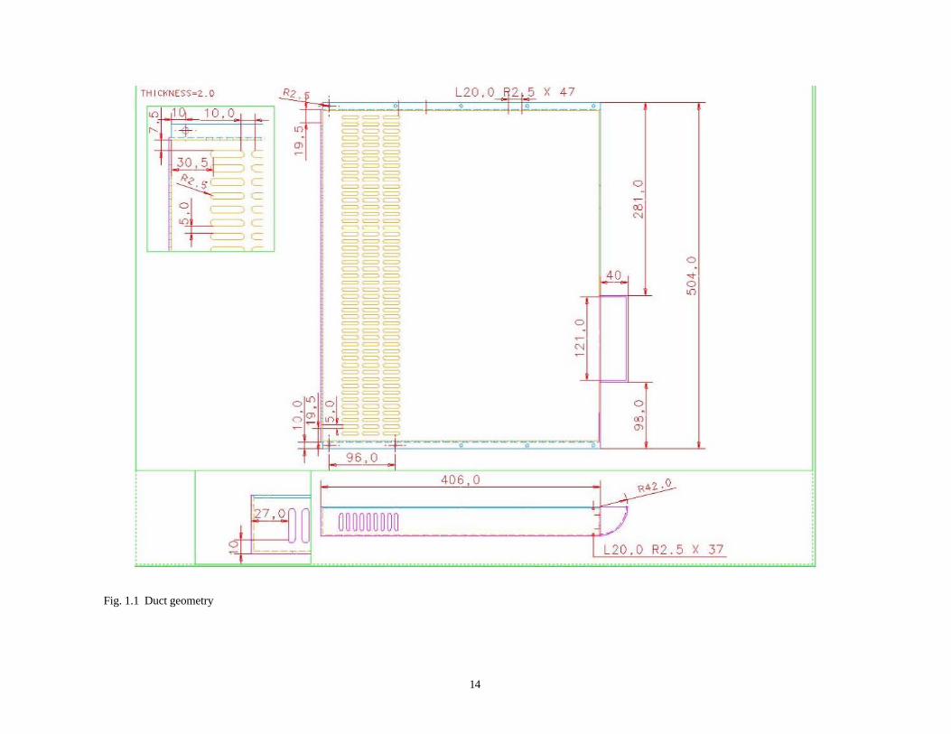
1.2 Condenser geometry Wind tunnel experiments were conducted on different condensers: cross-counterflow (C/F), spiral and

sawtooth (S/T ). The specifications of these condensers are listed in Table 1.1. When performing experiments,

these condensers were placed in ducts. A sketch of the duct is shown in Fig. 1.1. This duct has three rows of holes

that allow air to flow from bottom. A portion of air enters the duct from the front of the duct and as it flows over the

coil, incoming air from the bottom rows of holes gets mixed with it, the pressure differential of air-flow providing

the suction force needed to pull the air from the bottom holes. Based on their measurements, manufacturer estimated

that about 30% of the total air enters the duct from the front and the remaining 70% of the total enter through the

bottom of duct [19]. In the wind tunnel experiments, the air entrance holes on either side of the duct were closed.

The downwind end of the duct was mostly closed, except for the 121 mm gap where the fan would be positioned,

which guided the outgoing air to the nozzle for air-flow measurements. To simulate this unique air-flow

arrangement, basic finite element simulation model was developed, as described in the next few sections.

13

Table 1.1 Specifications of condensers

ET-Basic C/F#1 C/F#2 C/F#3 Spiral#1 Spiral #2 Spiral#3 S/T#1 S/T#2

Leg length (mm) - 465 465 465 410 410 410 468 468

Tube pitch (mm) 20 20 20 20 30 35 40 20 20

Row 9 2 2 2 1 1 1 1 1

Step 10 19 18 18 12 10 8 24 24

Fin number 260 1596 1512 2088 908 764 613 86 122

Fin thickness (mm) 1.6 1.6 1.6 1.6 0.35 0.35 0.35 1.6 1.6

Fin pitch (mm) 10(5) 10 10 7 6 6 6 10 7

Fin length (mm) - 33 33 33 - - - 474 474

Tube length (m) 15.51 19.47 18.49 18.49 5.47 4.73 3.88 11.93 11.93

Tube O.D.(mm) 4.76 4.76 4.76 4.76 4.76 4.76 4.76 4.76 4.76

Tube thickness (mm)

0.7 0.7 0.7 0.7 0.7 0.7 0.7 0.7 0.7

Heat transfer area(m2) (air/ref-side)

0.464/ -

0.562/ 0.205

0.533/ 0.195

0.631/ 0.195

1.037/ 0.058

0.898/ 0.050

0.735/ 0.041

0.384/ 0.126

0.470/ 0.126

Duct height (mm) - 40 40 40 25 25 25 35 35

14

Fig. 1.1 Duct geometry

TH ltKNESS- t . O R2. L20 . 0 ~ 2 5 X 47

1 10 , 0 • • • ~ .

~~~

~ :t- ~ ~ = - - --'" 30. 5 1-

. ~ - , ~

'2 . - . .. ~~ . ~~~ 0

- c:-= =-= =

:;1 ~ ~ "-'-=~= ~

~~~ 00 ~~~ N

<

, 0 .

--- ..±o. .. ~~~ 0 c=.== === "' ~~~

~~=

~~= =~~ 0 --- -,

~

~ N ~

---~~~

=~= ~-~

0 ": =~~ ~-= 0

~~ . ~ - -m _ 00

. - = '" ----- - -----~

'1 96 . 0

40 6,0 R'!\'2 ,O

27 . 00[ 000000000 ./

S L20. 0 R2 . 5 X 37

15

1.3 Simulation models Different simulation models were developed for the three different condensers. The vertical cross-

counterflow and spiral type condensers have similar features. The cross-parallel flow sawtooth coil simulation has

variations and is described separately.

1.3.1 Cross-counterflow condensers A vertical cross-counterflow coil and air-flow arrangement is shown in Fig. 1.2 to illustrate the features: a

number of identical elements consisting (in this case) of two tube passes and 84 wires welded to the front and back

of the tubes.

A i r F low

Fig. 1.2 Vertical Cross-counterflow coil and Air Flow

This was divided into a number of finite element divisions equal to the number of layers (slabs) in the coil.

Each element was modeled as a cross-flow heat exchanger using the effectiveness-NTU method:

( )in,ain,rmin

actual

maxmin

actual

max

actual

TTCQ

TCQ

QQ

e−

=∆

== (1.1)

Cmin is the minimum heat capacity between refrigerant and air (for some single phase elements, Cmin

corresponds to the refrigerant stream heat capacity). For specific heat exchanger conditions (i.e. geometry, type of

flow) the effectiveness can be related to the size of the heat exchanger through the number of transfer units (NTU).

minCUA

NTU = (1.2)

By using the effectiveness-NTU method and providing an initial guess for the refrigerant outlet state, it is

possible to simulate the entire condenser by solving the hundreds of equations in a sequential manner. This series of

equations is contained in a single procedure, which employs the upstream marching algorithm suggested by

Harshbarger and Bullard [20]. The refrigerant exit state is passed to this procedure from the main program. From

this condenser exit state, the inlet state of the refrigerant to that element is obtained. The effectiveness-NTU method

16

is used to determine the amount of heat transfer in that element. The refrigerant pressure drop is determined within

the element. Thus, the refrigerant properties at the exit from the upstream element are obtained.

Marching upstream in this fashion, the refrigerant properties (Tdis, Pdis) at the inlet to the condenser are

calculated and returned to the main program. If the calculated refrigerant state is not exactly equal to the actual

refrigerant inlet state, the above steps are repeated using some updated condenser exit state, after executing a

Newton-Raphson algorithm in the main program using Engineering Equations Solver [18]. If there is phase change

in an element from superheated to two-phase zone, the element is broken into two elements; the lengths of

superheated and two-phase zones within that element are determined using single 1-D Newton-Raphson algorithm

simulated within the procedure. The heat transfer and refrigerant pressure drop, etc. are then determined

accordingly. For detailed description of this algorithm, refer to [20].

The number of elements where air enters from the bottom is calculated using:

Numelm,hole =( Numelm *Depthhole/Depth) (1.3)

where

Numelm,hole = number of element allowing air-flow from bottom,

Numelm = total number of elements (= number of slabs),

Depthhole = depth of duct from front to the point where the last row of holes end,

Depth = total duct depth.

If this number is non-integer, it is rounded to the next higher integer. The amount of air entering from the front of

the duct is assumed to be 30% of total (as specified in [19]). The remaining 70% air from the bottom is equally

divided among the number of elements having holes at the bottom.

The air-side pressure drop across each element is multiplied by the number of elements and the total air-

side pressure drop is computed. The duct pressure drop of the rectangular duct is calculated and added. The

calculations neglect the pressure drops across the front grille and, due to turning of air to converge at the hole where

fan is located (Fig. 1.1). The simulations also neglected the bypass effect of air flowing over the return bends where

no wires are present.

The refrigerant pressure drop in each element is added up to obtain the total pressure drop. Usually, the

pressure drop in two-phase forms the largest component of the total pressure drop. The entrance and exit lengths of

the tube were neglected in the pressure drop computations and also in heat transfer, because, they formed a small

fraction of the total tube length (1 m in 19 m for C/F#1 coil). Similarly, the total heat transfer is obtained by

summing the heat transfer occurring in each element.

For wire-on-tube condensers, wires act as fins, so the fin efficiency (ηw) must be taken into account. In

Hoke, et al [21], it has been shown that,

mmtanh

? w = (1.4)

17

ww

2tw2

DkSh

m = (1.5)

The correlations used to determine the value of hw are geometry-specific and therefore are given separately for each

condenser. The surface resistance (Rsurf) is given by

weffsurf hA

1R = (1.6)

where

wwwt

teff A?

DD

AA += (1.7)

The overall UA is given by

ri,tweff

rsurf

hA1

hA1

1RR

1UA

+=

+= (1.8)

The air-side correlations is calculated from Nusselt number as a function of Reynolds number. Where

w

www k

DhNu = (1.9)

and kw was set to 60.5 W/m-K for steel wires.

In two-phase, effectiveness is related to NTU by,

-NTUe-1e = (1.10)

Also from Incropera and DeWitt [22], for single phase, the effectiveness for heat exchanger in cross-flow

with both fluids unmixed, is given by,

( ) ( )[ ]{ }

−−

=ε 1NTUCexpNTU

C1

exp-1 78.0rat

22.0

rat

(1.11)

The single-phase refrigerant-side heat transfer coefficient is calculated by Dittus-Boelter [23]. The

correlation developed by Dobson and Chato [24] for low mass fluxes is used to calculate the two-phase refrigerant

heat transfer coefficient. Refrigerant-side pressure drop in the two-phase region is calculated using Souza and

Pimenta [25], and the Darcy friction factor [26] in the single-phase (subcooled and superheated) region.

Thus, the common features to all cross-counterflow condensers have been discussed. The next subsections

discuss the specific features of simulations of vertical layer and spiral condensers. The simulation results are

compared with the experimental results.

18

1.3.1.1 Vertical cross-counterflow condenser For this condenser, the air-side heat transfer and pressure drop is computed by the correlation developed by

Lum and Clausing [27] with the angle of attack 90o. The air-side heat transfer coefficient is computed using

equation (1.12)

5744.0maxRe *CNuw =

( ) ( )2p

a4p

a3775.0a014.1expasin502.0C 2 ≤≤+−= (1.12)

The air-side pressure drop across the condenser is computed using equation (1.13)

=∆ 2

maxaDc,a V?21

CP

06533.0max21D Re DDC −+=

2p

a4p

)3229.0177.1exp()sin(7856.0D 21 ≤≤α−αα−=

2p

a4p

)2858.0exp()sin(451.2D 2 ≤≤αα=

µDV?

Re wmaxmax =

ratioface

max

min

face VVV

AA

≡=

( )

−

−−

=

tw

wwt

w

wratio

SSDSD

SD

1

1V

(1.13)

Wind tunnel experiments were conducted by Park et al. [19] for the test conditions listed in Table 1.2. The

results obtained for this vertical cross-counterflow condenser are compared with the experimental results in Tables

1.3 thru 1.5. Air flow rates greater than 1 m3/min result in face velocities exceeding 1 m/s (through the front grille),

which could create problems related to dust entrainment. Also at high flow rates, fan noise becomes a potentially

serious problem. Note, however, in the simulations, that the refrigerant exit temperature difference was pinched at

the two higher air-flow rates. Therefore, the higher air-flow rate simulations have not been conducted/reported. The

experimental results confirm that only 170W (calculated using (T,P)dis =(65oC,1030 kPa) and (T,P)exit =(30oC,1030

kPa) and refrigerant mass flow rate = 3 kg/h, neglecting refrigerant-side pressure drop) heat can be extracted from

the refrigerant by increasing air flow, due to pinching at the exit. Adding either area (A) or enhancing heat transfer

19

(h) is not going to be helpful, because pinched condition implies that hA → ∞ and the heat capacity of the

refrigerant stream has been reached. The measured air-side pressure drop is lower than what was predicted by the

simulations. This was not expected, since the simulations include only the duct and condenser pressure drop and

neglect the pressure drops due to front-grille and due to turning to converge at the hole where fan is located (Fig.

1.1). The experimental uncertainty of the air-side pressure drop measurements is not known.

The general trend of the results is that the capacity results are overpredicted by around 5% by the

simulation model. Air flow nonuniformities caused by the blockage at the rear of the duct, neglected in the

simulations, may account for a significant but unknown fraction of this difference. Uncertainty calculations in

experimental results can be found in Appendix B.

Table 1.2 Test conditions

Parameters Conditions Air inlet temperature (oC) 30 Refrigerant inlet temperature (oC) 65 Refrigerant flow rate (kg/h) 3.0 Refrigerant inlet pressure (kPa) 1030

Table 1.3 Vertical cross-counterflow simulation Results(C/F#1)

Results Parameters

Computed Experimental

Air flow Rate (m3/min) 0.67 0.97 1.43 1.90 0.67 0.97 1.43 1.90 Capacity (W) (air/ref-side)

113 145 171 108/ 111

143/ 139

166/ 165

170/ 166

∆Pair (mmH2O) 0.50 0.96 1.80 0.34 0.67 1.44 2.57 ∆Pref (kPa) 12 10 7.4 * * * * Exit quality 0.33 0.11 - 0.35 0.14 - - Tref,cond,out (°C) 40 40.1 30 40 40 35 33.7 Tair,cond,out (°C) 38.6 37.7 36.1 * * * *

- sub-cooled condenser exit * data not available

20

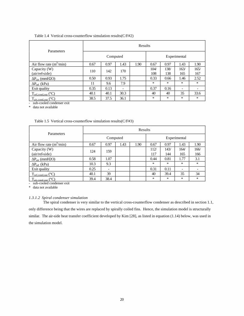
Table 1.4 Vertical cross-counterflow simulation results(C/F#2)

Results Parameters

Computed Experimental

Air flow rate (m3/min) 0.67 0.97 1.43 1.90 0.67 0.97 1.43 1.90 Capacity (W) (air/ref-side)

110 142 170 104/ 108

138/ 138

163/ 165

165/ 167

∆Pair (mmH2O) 0.50 0.93 1.75 0.33 0.66 1.46 2.52 ∆Pref (kPa) 11 9.6 7.9 * * * * Exit quality 0.35 0.13 - 0.37 0.16 - - Tref,cond,out (°C) 40.1 40.1 30.3 40 40 35 33.6 Tair,cond,out (°C) 38.5 37.5 36.1 * * * *

- sub-cooled condenser exit * data not available

Table 1.5 Vertical cross-counterflow simulation results(C/F#3)

Results Parameters

Computed Experimental

Air flow rate (m3/min) 0.67 0.97 1.43 1.90 0.67 0.97 1.43 1.90 Capacity (W) (air/ref-side)

124 159 112/ 117

143/ 144

164/ 165

166/ 166

∆Pair (mmH2O) 0.58 1.07 0.44 0.81 1.77 3.1 ∆Pref (kPa) 10.3 9.3 * * * * Exit quality 0.25 - 0.31 0.11 - - Tref,cond,out (°C) 40.1 39 40 39.4 35 34 Tair,cond,out (°C) 39.4 38.4 * * * *

- sub-cooled condenser exit * data not available 1.3.1.2 Spiral condenser simulation

The spiral condenser is very similar to the vertical cross-counterflow condenser as described in section 1.1,

only difference being that the wires are replaced by spirally coiled fins. Hence, the simulation model is structurally

similar. The air-side heat transfer coefficient developed by Kim [28], as listed in equation (1.14) below, was used in

the simulation model.

21

µρ oh

o

h

th

p

hoh

o

h

h

thpho

DVfinwithoutdiamterouterTubeD

heightFinF

thicknessFinF

pitchFinFFDdiameterHydraulicD

DF

F

FF

kDh

Nu

max

083.0763.0

551.0

Re

::

:

:)*2(:

Re414.0

=

+

−==

−

(1.14)

The air-side area is computed as the total fin and tube area. With this heat transfer coefficient, the effective

air-side area is calculated using equation (1.15).

)(*))1(*)/(1( wtfinwtweff AAAAAA +−+−= η (1.15)

The subscripts t and w indicate tube and fin areas respectively. The fin efficiency is calculated using radial

fin efficiency expression developed by Kraus et al. [29].

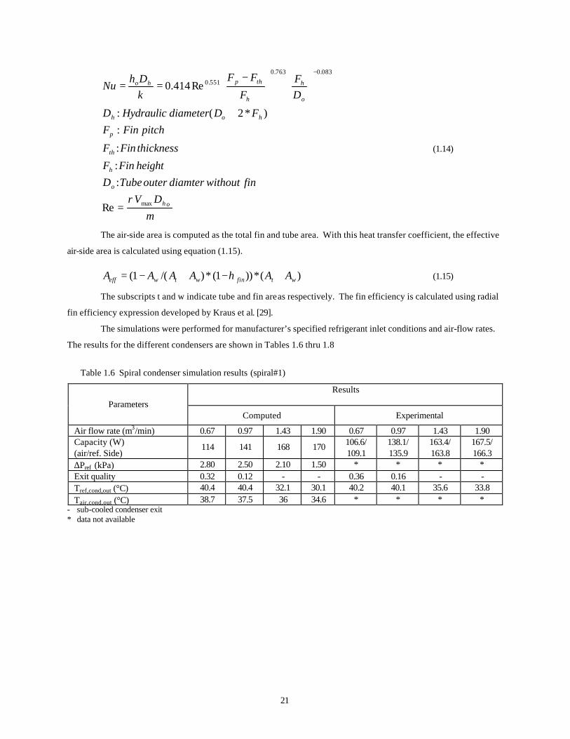
The simulations were performed for manufacturer’s specified refrigerant inlet conditions and air-flow rates.

The results for the different condensers are shown in Tables 1.6 thru 1.8

Table 1.6 Spiral condenser simulation results (spiral#1)

Results Parameters

Computed Experimental

Air flow rate (m3/min) 0.67 0.97 1.43 1.90 0.67 0.97 1.43 1.90 Capacity (W) (air/ref. Side)

114 141 168 170 106.6/ 109.1

138.1/ 135.9

163.4/ 163.8

167.5/ 166.3

∆Pref (kPa) 2.80 2.50 2.10 1.50 * * * * Exit quality 0.32 0.12 - - 0.36 0.16 - - Tref,cond,out (°C) 40.4 40.4 32.1 30.1 40.2 40.1 35.6 33.8 Tair,cond,out (°C) 38.7 37.5 36 34.6 * * * *

- sub-cooled condenser exit * data not available

22

Table 1.7 Spiral condenser simulation results (spiral#2)

Results Parameters

Computed Experimental

Air flow rate (m3/min) 0.67 0.97 1.43 1.90 0.67 0.97 1.43 1.90 Capacity (W) (air/ref. Side)

107 129 156 169 90.9/ 95.6

116.1/ 115

146.7/ 144.3

163.8/ 164.2

∆Pref (kPa) 2.60 2.10 1.80 1.40 * * * * Exit quality 0.39 0.21 0.01 - 0.46 0.32 0.10 - Tref,cond,out (°C) 40.4 40.4 40.4 30.7 40.1 40.1 39.6 35.4 Tair,cond,out (°C) 38.2 36.8 35.6 34.6 * * * *

- sub-cooled condenser exit * data not available

Table 1.8 Spiral condenser simulation results (spiral#3)

Results Parameters

Computed Experimental

Air flow rate (m3/min) 0.67 0.97 1.43 1.90 0.67 0.97 1.43 1.90 Capacity (W) (air/ref. Side)

92 112 136 154 90.4/ 91.8

112.9/ 110.9

141.6/ 138.4

161.5/ 161.5

∆Pref (kPa) 2.50 2.10 2.0 1.60 * * * * Exit quality 0.49 0.34 0.16 0.03 0.49 0.35 0.15 - Tref,cond,out (°C) 40.4 40.4 40.4 40.4 40.3 40.1 39.9 37.6 Tair,cond,out (°C) 37 36 34.9 34.2 * * * *

- sub-cooled condenser exit * data not available

1.3.2 Sawtooth condenser simulation The geometry of sawtooth condenser and airflow arrangement are shown in Fig. 1.3. Manufacturer’s

condensers did not have any clearance; hence, condenser amplitude was equal to the duct height.

For analysis of this heat exchanger, two zones were considered: two-phase and superheated. Each zone

was further subdivided into 4 elements (3 elements having one row of holes at the bottom and 4th element having no

holes). The data supplied for the ratio of airflow from the bottom to the airflow from the front (7/3) was used in this

analysis. Each element was modeled using effectiveness-NTU method as cross-flow heat exchanger with both

fluids unmixed. For modeling single-phase zones of such condensers, Barnes and Bullard [30] have used the

assumption of parallel-counterflow. However, in these simulations, detailed representation of airflow patterns was

needed, so approximations were made for modeling the refrigerant side. The refrigerant-side heat transfer coefficient

in both single and two phase were found out using the correlations described in earlier section 1.1 Simulation of

vertical cross-counterflow condenser. In the open literature, only Petroski and Clausing [2] have developed

correlations for airside heat transfer coefficient and pressure drop across the condenser. Accordingly, the air-side

heat transfer coefficient was obtained from the following Nusselt number definition.

23

667.0maxw Re 112.0Nu =

(1.16)

The air-side pressure drop (across the condenser alone) can be found using equation (1.17).

=∆ 2

maxDc,a V?21

CP

603.0maxD Re7.72C −= (1.17)

a) Top view b) Side view

amp

α=60°

HL

W

Air Flow

c) Photo of sawtooth condenser

Fig. 1.3 Sawtooth condenser configuration and airflow arrangement

The definitions for maximum velocity and Reynolds number are similar to those in equations (1.11) above.

Petroski and Clausing [2] has obtained these correlations based on sawtooth condensers having 7-9 layers. The

number of layers in condenser prototypes simulated here were larger than these, hence, corrections were applied to

the pressure drop across coil as given in equation (1.18).

7*

)60(

*2

,layers

cacorrected

layers

NPP

SinHeight

DepthN

∆=∆

=

(1.18)

24

The number of layers is related to the depth and height of the condenser through the sawtooth angle (60o)

from the data supplied by the manufacturer [19]. The total pressure drop across the condenser is the weighted sum

(over the condenser depth) of the condenser pressure drop across each element. The duct pressure drop is computed

corresponding to the duct depth for each element. Again, the pressure drop across the front grille is neglected in

these computations. The results of these simulations for condensers S/T#1 and S/T#2 are presented in Tables 1.9

&1.10 respectively. One interesting observation is that the experimental measurements of air-side pressure drop are

lower than those predicted by the simulation model. This is unexpected because, the measurements included

pressure drop across the front grille and the pressure drop experienced by air due to turning at the back plate to

converge to the hole for the fan.

Table 1.9 Sawtooth condenser simulation results (S/T#1)

Results Parameters

Computed Experimental

Air flow rate (m3/min) 0.67 0.97 1.43 1.90 0.67 0.97 1.43 1.90 Capacity (W) (air/ref-side)

90.1 116 149 179. 99.7/ 101.6

128/ 123.6

160.4/ 161.3

170.9/ 167.6

∆Pair (mmH2O) 0.78 1.3 2.25 3.34 0.34 0.67 1.48 2.56 ∆Pref (kPa) 6.5 6.4 6.4 6.4 22 26 19.6 12 Exit quality 0.50 0.31 0.07 - 0.42 0.26 - - Tref,cond,out (°C) 40.2 40.3 40.3 40.3 39.7 39.6 38.4 32.3 Tair,cond,out (°C) 37 36.2 35.4 34.7 36.8 36.2 35.3 34.2

- sub-cooled condenser exit

Table 1.10 Sawtooth condenser simulation results (S/T#2)

Results Parameters

Computed Experimental

Air flow rate (m3/min) 0.67 0.97 1.43 1.90 0.67 0.97 1.43 1.90 Capacity (W) (air/ref-side)

106 136 177 213 106/ 108

138/ 136

166/ 167

167/ 169

∆Pair (mmH2O) 0.88 1.5 2.5 3.76 0.4 1.0 1.6 2.8 ∆Pref (kPa) 6.5 6.4 6.4 6.4 21 26 14 7 Exit quality 0.39 0.16 - - 0.37 0.17 - - Tref,cond,out (°C) 40.3 40.3 40.3 40.3 39.7 39.6 38.4 32.3 Tair,cond,out (°C) 38.1 37.2 36.3 36 37.3 36.7 35.5 34.2

- sub-cooled condenser exit

1.4 Air-side pressure drop assumptions The experimental results on the air-side pressure drop of the manufacturer’s condensers include in addition

to duct and condenser pressure losses, the pressure drop across the front grille and the pressure drop experienced by

air due to turning to converge at the hole where the fan is located. In their domestic refrigerators, in addition to

these losses the fan has to perform extra work to pull the air across the compressor also. The results of the

simulation do not include these additional components of air-side pressure drop. In this section, the air-side pressure

25

drop due to front grille is computed for the air-flow rates considered by the manufacturer in their experiments. The

manufacturer’s front grille is (40 mm x 484 mm). It has 45 holes (length = 20.0 mm, breadth = 5 mm and 2.5 mm

radii on both ends). Only 30% of the total air flows across this front grille. Based on this, the air velocity through

each hole is first computed. The holes are treated as orifices in a plate. Reynolds number was evaluated based on

the inlet flow rate. For laminar air flow, the following formula for Cd was used for computations of pressure drop

from Idelchik [31].

32 Re2

Re2

Re2

2dcb

a +++=ϕζ

2Re Re*1Re*11 cbaD ++=−ε

22Re /)]707.1([ ffC Dd −+= −εζ ϕ

(1.19)

f = area of holes/area of front plate. The seven parameters in the above curve fits of functions of Re were obtained

by doing a least squares fit of these parameter values given in Idelchik [31] over the Reynolds number range of

interest (60 thru 1000). The grille pressure drop was computed as follows.

2***2/1 VCP dgrille ρ=∆ (1.20)

The values obtained for various air-flow rates have been listed in table 1.11 The exit pressure drop is computed from

the following expression of pressure drop for (air flow from conduit of one size to another, with Re<105) from [31].

The relevant equations are:

100

2200

Re0,

/1*707.01

)/(*

FF

FFC exitd

−+=

−+= −

ζ

ζεζ ϕ (1.21)

where,

F0 = hole area

F1/2 = cross-sectional area of conduit from where flow is (leaving/entering)

In these computations, hole area is assumed to be equal to the area of conduit where air is entering. (i.e. F0 = F2). In

[31], tables are available for computing the parameters ζϕ and also for (ε0)-Re as a function of Reynolds number and

F0/F1. Substituting the values for different flow rates and (F0/F1 = 121X40/484X40 = .25), the exit pressure drop has

been calculated.

Table 1.11 Additional pressure drop

Air Flow Rate (m3/min)

∆Pgrille (mmH2O)

∆Pexit (mmH2O)

0.67 0.4 0.12 0.97 0.8 0.26 1.43 1.6 0.55 1.9 2.5 0.97

26

The air flow rates listed in this Table are the manufacturer’s test conditions. Actually only 30% of this

enters through the front grille. For exit pressure drop computations, velocity is computed based on the total air flow

rates. From Table 1.11, it is seen that this additional pressure drop is about 60% larger (for C/F#1 condenser for the

lowest air-flow rate) than the total of condenser and duct loss.

1.5 Condenser performance in actual refrigerator The foregoing discussion is based entirely on simulations in wind tunnel. The test conditions in wind

tunnel experiments differ significantly from the actual refrigerator. Therefore, to account for difference in

performance of condensers in wind tunnel and actual refrigerator, additional experiments were performed in a

simulated machine room to replicate the fluid mechanics of the air flow beneath an actual refrigerator. In the

machine room, the air exiting from the fan has to flow over the compressor and through an exit grille. This

additional pressure drop increases fan power and decreases air flow rate. This, in turn, decreases the condenser

capacity. The machine room experimental results for the ET-basic and S/T#2 condensers (see Table 1.1 for

dimensions) are shown in Table 1.12.

Table 1.12 Machine room experimental results

Condenser Configuration Box-type Saw-tooth

Refrigerant flow rate (kg/h) 2.5 3.0 3.5 2.5 3.0 3.5 Inlet pressure (kPa) 1033 1034 1033 1033 1034 1034 Inlet temperature (oC) 65 65 65 65 65 65

Exit quality - 0.17 0.30 - - 0.23 Capacity (W) 137.2 135.8 138.0 138.7 160.5 148.4

Box type condenser ET-basic condenser in Table1.1 Sawtooth type condenser: S/T#2 condenser in table 1.1

2. Optimization of sawtooth condenser Optimization of sawtooth condenser was conducted using the same equations as the simulation model

developed in section 1.3. Detailed descriptions of the optimization are given in this section of the report.

2.1 Simulation of wind tunnel experiments The dimensions of two prototype sawtooth heat exchangers are described in Table 1.1. Inlet air and

refrigerant conditions are specified in Table 1.2. The simulation results are compared to the manufacturer’s

experimental results from wind tunnel tests earlier in this report. Since the refrigerant-side capacity calculations are

all based on measurements obtained with immersion RTD’s and a mass flow rate maintained at 3.0 kg/h for all the

tests , they are expected to be more consistent than calculations based on air side measurements. At (air-flow rate =

1.43 m3/min) 168 W (from [19]), heat rejection from the baseline condenser in the wind tunnel is greater than

prototype ST#1 (149 W) and slightly less than ST#2 (177 W) as seen from the simulation results in Tables 1.9-10.

According to the wind tunnel tests, the new prototype condensers fail to provide substantial performance

improvement over that of the baseline unit. However this is not the case in practice. When installed in a

refrigerator, the baseline condenser is not well ducted, because flow configuration is not uniform due to the defrost

water pan located at the bottom of condenser and oblique air entrance to the condenser. The inlet air enters the

condenser from the backside of refrigerator and flows perpendicular to entrance direction through the condenser and

27

compressor and exits to the backside. Thus performance is degraded due to air bypass effects, and the resulting

refrigerant exit quality is greater than zero. Downstream, a hot wall condenser (cluster) is therefore needed to

complete the condensation process. Because of the superior ducting in the wind tunnel, however, the baseline

condenser rejects enough heat to subcool the outlet about 6°C. The prototype condensers, on the other hand, are

designed to fit in a duct under the front of the refrigerator, allowing the machine compartment to be downsized to

enlarge the food storage volume. Since the sawtooth prototypes would be installed in a duct similar to the wind

tunnel experiment, their performance in the actual refrigerator is expected to be the same as in the wind tunnel.

2.2 Simulation of compressor-condenser subsystem The wind tunnel experiments were conducted with identical inlet conditions [19], but the condenser outlets

were subcooled. Due to the subcooling differences, it is difficult to estimate potential contributions to cycle

efficiency. Although it is difficult to be certain without simulating the entire system, having a subcooled condenser

outlet is probably suboptimal – saturated liquid is probably a more reasonable design target because it maximizes the

two-phase area (and minimizes charge, which in turn minimizes cycling losses associated with charge migration).

Therefore a second set of simulations was conducted to compare the three condensers (baseline, ST#1 and ST#2),

with the compressor included within the subsystem boundary so the differences in compressor work could be

compared.

The compressor model was developed from manufacturer’s data as discussed in earlier sections of this

report. For this analysis it is assumed that the refrigerator is operating at the 30°C design condition where the

compressor inlet state, obtained from the manufacturer, is P = Psat(Te) where Te = -35°C, and Tsuc ~ 30°C) and the

evaporator exit is saturated vapor. The baseline cycle was simulated in the following manner, with the result shown

in Figure 2.1. Based on the manufacturer’s data for the baseline coil for air-flow rate = 1.43 m3/min, an approximate

value for the air-side heat transfer coefficient was extracted using a simple multi-zone model of the condenser. This

was then used to simulate the baseline cycle with specified compressor inlet condition with the condenser exit fixed

to be saturated liquid, yielding the compressor outlet pressure. The fan power was assumed to be constant at 2.16

W. The various parameters are reported in Table 2.1, and results of a simple thermodynamic state point analysis are

shown in the P-h diagram. The total refrigerant pressure drop was assumed to be 1 C.

28

Table 2.1 Prototype condenser simulation

Results Parameters

Baseline S/T#1 S/T#2

Air Flow Rate (m3/min) 1.43 1.43 1.43

Condenser Capacity (W) 157.7 153 158

Evaporator capacity (W) 146 142 147 Fan power (W) 2.16 2.16 2.16 Compressor power (W) 125.6 125 125.2 COP 1.144 1.121 1.155 Refrigerant Mass Flow Rate (kg/h) 3.0 2.95 3.0

Tdis (oC) 62.5 63.2 62.9

Tcond (oC) 39.3 40.8 39.2

62.5oC39.3

oC

h

P

Refrigerant Flow Rate = 3.0 kg/hCondenser Capacity = 157.7 WEvaporator Capacity = 146 WCompressor Power = 125.6 WQcomp = 114 W

-35 o

C

30 oC

Fig. 2.1 Refrigeration Cycle on P-h diagram

The results show that the ST#2 design offers negligible performance improvement over the baseline design.

This was not surprising because the wind tunnel experiments [19] showed that the baseline and S/T#2 coils

exhibited approximately the same heat transfer capacities. Recall that the baseline coil was positioned in the wind

tunnel such that no air bypassed the coil, hence its performance was better than in the actual refrigerator. Upon

closer inspection, however, there are reasons to expect that the higher heat transfer coefficient of the sawtooth

design should have improved performance, even in the wind tunnel. The heat transfer areas of these two coils are

29

same (Table 1.1). From the wind tunnel data, the air side heat transfer coefficient was found to be 55 W/m2-K,

compared to 69 W/m2-K for the ST#2 heat exchanger. The explanation is clear. The higher h of the sawtooth coil

was exploited to produce a packaging advantage: allowing 70% of the air to enter the duct from the bottom, so it

passed over only part of the heat exchanger. That explains why the overall Q’s were the same, despite the large

difference in air side heat transfer coefficient. There were also slight differences between the two heat exchangers

on the refrigerant side: tube length was ~20% greater for the baseline coil (Table 1.1). However, the teeth in the

saw-tooth coil produce a higher refrigerant-side pressure drop (associated with turning of the refrigerant and perhaps

also due to gravity).

These simulations and wind tunnel results both illustrate how the prototype ST#2 outperforms ST#1. The

slightly higher refrigeration capacity provided by ST#2 means that the refrigerator should pull down more quickly. It

should also have slightly shorter runtimes than the baseline, even if perfect ducting of the baseline unit enabled it to

perform as well in a refrigerator as it did in the ducted wind tunnel test. The results are directly comparable, except

that the sawtooth simulations account for refrigerant-side pressure drop while the baseline calculation neglects it (a

small effect, affecting condenser heat transfer by only about 1Watt). The additional benefit of the sawtooth design,

of course, is that it allows for improved packaging in the machine room, and therefore enlargement of the

refrigerated space.

If a hot-wall condenser (cluster) were located downstream of the sub-condenser, it would have little effect

on the cycle at this design operating condition, because the additional (~ 3°C) subcooling in the cluster would

increase (by only ~2°C) the amount of subcooling occurring in the ctslhx (capillary tube suction line heat

exchanger), thus having only a small effect on evaporator inlet quality and hence refrigerant mass flow rate and

power. Therefore the foregoing simulations and the optimization analysis that follow are conservative, because they

neglect the presence of the cluster.

2.3 Optimization of sawtooth geometry The next step was to conduct an optimization analysis to find the best wire and tube diameters and spacings

for a sawtooth condenser designed to fit in the same package volume as the prototype units. The constraints on

optimization specified by the manufacturer are listed in table 2.2 below, along with slightly relaxed constraints used

by Barnes and Bullard [30] and the wire and tube sizes and spacings used by Petroski and Clausing [2] when

developing the air-side heat transfer and pressure drop correlations. The constraints listed under the column named

search are the manufacturer’s constraints [19]; and the constraints listed under the columns named Barnes and

Correlation are the constraints in [30] and [2] respectively. Constraints on wire diameter were not specified by

manufacturer, so the upper bound was arbitrarily set to 1.8 mm.

30

Table 2.2 Constraints on optimization Lower Bound Upper Bound

Barnes Search Correlation Variable

Correlation Search Barnes

- 15 25.4 Tube Pitch (mm) 25.4 20 -

4 4.2 4.8 Tube Diameter (mm) 4.8 4.76 7.95

1 7 4.8 Wire Pitch (mm) 6.4 10 10

0.9 0.9 1.22 Wire Diameter (mm) 1.6 1.8 1.8

- - - Tube –wall –thickness/diameter ratio=70/476

- - -

4 - - Tube –pitch/ diameter-ratio - - -

The same refrigerant and air inlet conditions are specified for the compressor/condenser subsystem

boundary: Psuc, Tsuc, Tamb, and the refrigerant outlet quality is fixed at x=0. Instead of specifying wire and tube

diameters and spacings, the optimization searches for the combination that maximizes system

compfan

e

WWQ

COP && += (2.1)

From the fan data provided by the manufacturer [19], a quadratic least squares curve fit was used to obtain

fan curve. Combined fan and motor efficiency was set to 12% (by using manufacturer’s data for fan power at air-

flow rate = 1.43 m3/min). Instead of specifying air flow rate, the optimal value is calculated from the fan curve, from

the air side pressure drop that varies with condenser geometry. The maximum COP was achieved when the addition

of heat transfer surface area reduced compressor power by the same amount as the fan power increased.

The optimal geometry is shown in column 1 of Table 2.3. The second column shows the effect of limiting

the search to the range of wire and tube dimensions that provided the experimental basis for developing the

correlation, thus avoiding extrapolation. The third column allows for significant extrapolation, expanding the search

domain over a broader range of dimensions suggested by manufacturers of wires and tubes (see Barnes & Bullard

[30]).

As expected, the highest COP was obtained by expanding the search domain to that specified by Barnes

[30]. Given the packaging constraints, it appears that performance is optimized by using smaller diameter tubes and

spacing them closer together, with large diameter wires spaced more closely than ST#2. The closely spaced wires

would increase air side pressure drop, so the air flow rate was reduced to minimize the fan power penalty. As a

result, the outlet air temperature increased to the point where it almost equals the condensing temperature (see

column 3 of table 2.3). Any lower air flow rate would have required a higher condensing temperature, thereby

decreasing COP. Basically, the optimization algorithm sought to improve the condenser by adding surface area, and

by reducing air flow rate to the minimum. Whether search constraints or Barnes constraints [30] are used, the COP

is about the same, thus, the configuration listed in column 1 of the table 2.3 is optimal under these circumstances.

31

Table 2.3 Results of optimization (constant fan efficiency)

Parameter Max COP (Search

Constraints)

Max COP (Correlation constraints)

Max COP (Barnes’

Constraints) ST#2

COP 1.136 1.12 1.139 1.11 Evaporator Capacity (W) 145 142 145. 142 Total Power (W) 127.6 127.4 127.5 127.3 Compressor Power (W) 125 125 125 124.8

Fan Power (W) 2.55 2.54 2.5 2.5 Condenser Capacity (W) 155.3 152 156 151.8 Air Flow Rate (m3/min) 1.06 1.04 0.9 1.08 Tube Diameter (mm) 4.2(-) 4.8(+/-) 4(-) 4.76 Wire Diameter (mm) 1.8(+) 1.6(+) 1.8(+) 1.6 Tube Spacing (mm) 15(-) 25.4(+/-) 16 20 Wire Spacing (mm) 7(-) 4.8(-) 4 7 Tcond (

oC) 39.8 40.9 39.8 41 Tair,out (

oC) 37.5 37.5 38.9 37.2 Acond (m2) 0.534 0.495 0.62 0.47 Mass (kg) 2. 1.75 2. 1.72 D Pref (kPa) 15.5 4.7 18.5 6.1 D Pair (mmH2O) 1.8 1.8 1.93 1.73 Tdis (

oC) 63.1 63.2 63.1 63.2 (-)=> value at lower bound (+)=> value at upper bound

2.4 Effect of constant fan power For all the optimizations described in section 2.3 above, the compressor power was computed using the

compressor map for the Samsung ZK180b. The combined fan-motor efficiency was assumed constant at 12% and

fan power was calculated for each combination of airflow and pressure drop.

At this point the authors began to question an assumption embedded in the model, namely that the

compressor fan/motor efficiency was constant. Data provided later by the manufacturer showed significant

variations in fan efficiency (manufacturer’s data [19] indicated that the fan power is fairly constant over a wide

range of air-flow rates and air-side pressure drops, hence, it was concluded that fan efficiency has to vary), so the

analysis was repeated using the constant power data (~2.16 W, for most of air-flow rates in the range of interest)

provided by manufacturer [19]. These data show that fan power is essentially independent of pressure drop, over the

relevant range of air flow rates. The revised results are shown in table 2.3a below. The authors expected further

addition of area when fan power penalty is kept constant. The results in table 2.3a, however, indicate that further

addition of area is precluded by the requirement of certain air-flow rate to condense the refrigerant. Hence, these

results are very similar to the ones listed in table 2.3, the slight improvement in COP is observed only because of

reduction in fan power penalty.

32

Table 2.3a Results of optimization (constant fan power)

Parameter Max COP (Search

Constraints)

Max COP (Barnes’

Constraints)

COP 1.14 1.141 Evaporator Capacity (W) 145 145.1 Total Power (W) 127.2 127.2

Compressor Power (W) 125 125

Fan Power (W) 2.16 2.16 Condenser Capacity (W) 155.3 156 Air Flow Rate (m3/min) 1.06 0.9 Tube Diameter (mm) 4.2(-) 4(-) Wire Diameter (mm) 1.8(+) 1.8(+) Tube Spacing (mm) 15(-) 16 Wire Spacing (mm) 7(-) 4 Tcond (

oC) 39.8 39.8 Tair,out (

oC) 37.5 38.9 Acond (m2) 0.534 0.62 Mass (kg) 2 2.24 D Pref (kPa) 15.5 18.4 D Pair (mmH2O) 1.77 2 Tdis (

oC) 63.1 63.1 (-)=> value at lower bound (+)=> value at upper bound

2.5 Optimization of sawtooth condenser in cross-counterflow arrangement Based on earlier work conducted at ACRC, (see [2], [27] and [30]) it was expected that the vertical cross-

counterflow condenser would give the best performance. For manufacturing reasons, however, the sawtooth

condenser is desirable because it is possible to exploit the higher air-side heat transfer coefficient at lower duct

heights, thus leading to an overall increase in the refrigerator compartment volume. The results of optimization of

sawtooth condenser when air-flow is parallel to tubes are presented in Sections 2.3-4. It was decided to explore the

sawtooth condenser by placing it in air-flow configuration similar to the vertical cross-counterflow arrangement.

The simulation model, described in an earlier section 2.1 was used for this purpose. The only changes made were to

the air-side heat transfer and pressure drop correlations [2]. The geometry calculations, too, were different. The

same general dimensions of the duct were used. Optimization was carried along similar lines as for optimization of

the sawtooth condenser.

A four dimensional search using EES [18] is inherently complex task. This is further complicated by the

finite element of nature of the algorithm used. Hence, from insights gained during earlier analyses, the optimal

configuration is expected to be the one that maximizes the heat transfer area. Hence the tube spacing was fixed at

the lowest bound and holding tube diameter constant at its upper bound, a two-dimensional search was carried out to

determine the optimal configuration. This led to the configuration with the lowest number of thickest wires.

Varying the diameter in the range specified by manufacturer’s constraints had no further effect on the value of COP.

33

The results of this optimization are presented in table 2.4 below. Since the heat transfer area is already at its

maximum, the optimization with fan power constant is unlikely to yield any further performance improvement.

This configuration seems to be only slightly better than the optimal configuration found out using sawtooth

condenser in cross-parallel flow configuration.

Table 2.4 Optimization of cross-counterflow sawtooth condenser

Parameter Max COP Configuration

(manufacturer’s constraints)

COP 1.163 Evaporator Capacity (W) 149.3 Total Power (W) 128.4

Compressor Power (W) 125.8

Fan Power (W) 2.6 Condenser Capacity (W) 161.3 Air Flow Rate (m3/min) 1.08 Tube Diameter (mm) 4.76(+) Wire Diameter (mm) 1.8(+) Tube Spacing (mm) 15(-) Wire Spacing (mm) 7(-) Tcond (

oC) 38.5- 38.0 Tair,out (

oC) 37.7 Acond (m2) 0.84 Mass (kg) 3.5 D Pref (kPa) 15.0 D Pair (mmH2O) 1.74 Tdis (

oC) 62.2

(-)=> value at lower bound (+)=> value at upper bound

2.6 Discussion of results The foregoing analysis was based on compressor performance data obtained at condensing temperatures

ranging from 40 to 48°C. The data points are shown in Fig. 2.2, along with curve fits produced with the standard

10-parameter polynomial equation. Note that the curve fit must be extrapolated to condensing temperatures less

than 40°C, and that the extrapolated curve appears to be physically unrealistic. This illustrates the risks of

extrapolating polynomials; they can fit very well within the range of actual data, but they embody none of the

physics governing compressor behavior.

34

1

1.3

1.6

1.9

-40 -35 -30 -25 -20 -15 -10

Te (oC)

CO

P

Expt (Tc=40) Curve fit(Tc=40) Expt(Tc=45) Curve Fit (Tc=45)Expt (Tc=48) Curve Fit (Tc=48) Curve Fit (Tc=35)

Fig. 2.2 COP vs Te at constant Tcond (polynomial fit)

Fig. 2.3 shows the curve fit obtained by Kim and Bullard’s semi-empirical model [3], which is essentially a

curve fit of physical parameters known to govern compressor operation. It does not fit the data quite as well inside

the range, but it appears to extrapolate to 35°C in a much more reasonable manner. Therefore Kim and Bullard’s

compressor model [3] was used for all the simulations and optimizations presented in this report. Fig. 2.3 was

obtained by calculating COPcomp from the original measurements of refrigeration capacity and power in the

compressor calorimeter. At -35°C evaporating temperature, power was essentially independent of condensing

temperature; it changed by less than 1% over the 40-48°C range of experimental data. The system COP

improvements shown in Tables 8 and 9, therefore, resulted from the capacity increase that was experienced as

condensing temperature was reduced. From the P-h diagram it can be seen that lower condensing temperatures

produce a more efficient cycle, by reducing compressor power per unit mass, and at the same time increasing the

refrigerating effect per unit mass by reducing evaporator inlet quality. Referring again to the optimization results, it

is clear that the condenser geometries improved system COP by improving the cycle (and therefore refrigerating

capacity), not by directly reducing compressor power.

35

1

1.1

1.2

1.3

1.4

1.5

1.6

1.7

1.8

1.9

2

-40 -35 -30 -25 -20 -15 -10

Te (oC)

CO

P

Expt (Tc=40) Kim(Tc=40) Expt(Tc=45) Kim(Tc=45)Expt (Tc=48) Kim(Tc=48) Kim (Tc=35)

Fig. 2.3 COP vs. Te at constant Tcond (Kim and Bullard [3])

Referring again to 35°C and 40°C curves in Fig. 2.3 it is apparent that condenser improvements can

increase COPcomp at any evaporating temperature. Moreover the percentage improvement rather small, and is nearly

independent of evaporating temperature. In contrast, substantial COPcomp increases could be obtained by improving

evaporator performance, raising Te from –35 to -25°C for example.

In summary, the simulations have illustrated how a sawtooth condenser could increase system performance,

given constraints on package volume and fan performance. System performance improvements resulted mainly

from reducing the condensing temperature – the compressor power remained almost constant while refrigerant mass

flow and system capacity increased, as heat transfer area was added to the condenser in a manner that minimized air

and refrigerant side pressure losses. The optimal design was reached when the added condenser area caused so

much pressure drop that the air flow rate dropped to the point where the air and refrigerant temperatures pinched.

As the temperature difference diminished, condenser mass, a surrogate for cost, began to rise rapidly. The

conclusion is that using a more powerful and efficient fan might be the most cost-effective way to achieve further

increases in condenser performance. That would allow air flow rate to be increased and the condensing temperature

reduced, and leave a slightly larger dT at the pinch point, assuming that the power requirement and noise generation

would not be excessive. It appears that noise and cost constraints will severely limit the potential for achieving

greater performance from wire-on-tube condenser design.

The primary benefit of the sawtooth condenser, compared to the baseline design, appears to come from

packaging rather than changes in heat transfer coefficient and surface area. The package volume is not only ducted,

but also allows for food storage volume to be increased.

Greater benefits, however, are likely to be obtained by efforts to improve evaporator performance. At

higher evaporating temperatures, substantial compressor power savings could be obtained. Moreover, warmer fin

surfaces collect less frost and therefore maintain better food quality and minimize defrost energy.

36

The optimal condenser configuration prescribed here was obtained using fan curve and air-side pressure

drop across duct and condenser alone. This analysis neglected the pressure drop across the front-grille, the turning

experienced by air to converge at the hole where fan is located, and pressure drops across the compressor and the

exit grille. As illustrated in section 1.4, these pressure drops could be major components of total pressure drop on

the air-side. However, certain trends are apparent from the optimizations presented in this chapter, and it seems

reasonable to assume that the same geometries and air flow rates would also be optimal if a slightly more powerful

fan were used to overcome the additional air side pressure drop. The prescribed condenser outlet condition

(saturated liquid) determines the condensing temperature. Then according to fan characteristic curve, the lowest air-

flow rate is calculated to avoid pinching. If air-side pressure drop rises substantially due to the downstream

obstructions, the optimal condenser may be more open (i.e. the condenser will have lower heat transfer area),

shifting the power requirement to the compressor and resulting in a slightly higher condensing temperature.

It is recommended that future experimental work focus on perfecting the “machine room experimental

technique” being developed by the manufacturer. With additional instrumentation to measure air flow rates, for

example, performance can be measured under realistic conditions. By including the compressor and exit grille, the

fan can be properly sized to achieve the desired air flow rate. By controlling the compressor suction state and using

a needle valve to control the condenser outlet at the saturated liquid state, the subsystem will adjust to the

condensing temperature that will be experienced in the actual refrigerator. Such an approach ensures optimal

matching of the condenser and compressor subsystem. The resulting mass flow rate determines the refrigerating

capacity, and hence the runtime fraction for the compressor chosen. The simulation and optimization modeling

presented here can help identify design strategies and near-optimal condenser configurations prior to conducting

such experiments.

37

References

[1] Nadel, S., 1997, “Appliance energy efficiency: opportunities, barriers, and policy solutions,” in Energy Efficiency in Household Appliances, Edited by P. Bertoldi, A. Ricci, and B. Huenges Wajer, Springer, pp. 22-37.

[2] Petroski, S.J. and Clausing, A.M., 1999, “An investigation of the performance of confined, saw-tooth shaped wire-on-tube condensers,” ACRC TR-153, University of Illinois at Urbana-Champaign.

[3] Kim, Man-Hoe and Bullard, Clark W., 2001, “A Simple Approach on the Thermal Performance Analysis of Small Hermetic Reciprocating Compressors,” ASHRAE Trans., Vol. 107, Part 1, pp. 109-119.

[4] Srichai, P.R. and Bullard, C.W., 1997, “Two-speed compressor operation in a refrigerator/freezer,” ACRC TR-121, University of Illinois at Urbana-Champaign.

[5] Kelman and Bullard, C.W., 1999, “Dual temperature evaporator refrigerator design and optimization,” ACRC TR-148, University of Illinois at Urbana-Champaign.

[6] Dabiri, A.E. and Rice, C.K., 1981, “A compressor simulation model with corrections for the level of suction gas superheat,” ASHRAE Transactions Vol. 87, Pt. 2, pp. 771-782.

[7] Mullen, C.E., Bridges, B.D, Porter, K.J., Hahn, G.W. and Bullard, C.W. 1998, “Development and validation of a room air conditioning simulation model,” ASHRAE Transactions Vol. 104, Pt. 2, pp. 389-397.

[8] Haider, I., Lavannis, M.K. and Radermacher, R., 1997, “Investigations of the EPA refrigerator analysis (ERA) software: compressor map and ambient temperature effects,” ASHRAE Transactions, Vol. 103, Pt. 11, pp. 608-618.

[9] Prakash, R. and Singh, R., 1974, “Mathematical modeling and simulation of refrigerating compressors,” Proceedings of the 1974 Purdue Compressor Technology Conference, pp. 274-285.

[10] Hiller, C.C. and Glicksman, L.R., 1976, “Detailed modeling and computer simulation of reciprocating refrigeration compressors,” Proceedings of the 1976 Purdue Compressor Technology Conference, pp. 12-17.

[11] Domanski, P.A. and Didion, D.A., 1983, “Computer modeling of the vapor compression cycle with constant flow area expansion device,” National Bureau of Standards, Building Science Series No. 155.

[12] Todescat, M.L., Fagotti, F., Prata, A.T. and Ferrerira, R.T.S., 1992, “Thermal energy analysis in reciprocating hermetic compressors,” Proceedings of the 1992 International Compressor Engineering Conference at Purdue, pp. 1419-1428.

[13] Cavallini, A., Doretti, L., Longo, G.A., Rossetto, L., Bella, B., and Zannerio, A., 1996, “Thermal analysis of a hermetic reciprocating compressor,” Proceedings of the 1996 International Compressor Conference, Purdue University, West Lafayette, Indiana, pp. 535-540.

[14] Rigola, J., Perez-Segarra, C.D., Oliva, A., Serra, J.M., Escriba, M. and Pons, J., 1996, “Parametric study and experimental comparison of small hermetic refrigeration compressors using an advanced numerical simulation model,” Proceedings of the 1996 International Compressor Engineering Conference at Purdue, pp. 529-534.

[15] Klein, S.A. and Reindl, D.T., 1999, “Develop data base for determining optimum compressor rating points for residential refrigerator and freezer compressors,” RP-870 Report, ASHRAE, Atlanta.

[16] Rasmussen, B.D., 1997, “Variable speed hermetic reciprocating compressors for domestic refrigerators,” Ph.D. Thesis, Technical University of Denmark.

[17] Kuehn, T.M., Ramsey, J.W. and Threlkeld, J.L., 1998, Thermal environmental engineering, 3rd edition, Prentice Hall.

[18] Klein, S.A. and Alvarado, F.L., 1999, Engineering equation solver, version 5.029, F-Chart Software.

[19] Park, S.K., Yang, K.Y., Chi, S.K., 2001, Private Communications.

38

[20] Harshbarger, D.S. and Bullard, C.W., 2000, “Finite Element Heat Exchanger Simulation Within a Newton-Raphson Framework.” University of Illinois at Urbana-Champaign, ACRC TR-171.

[21] Hoke, J.L, Clausing A.M. and Swofford T.D., 1997, "An Experimental Investigation of Convective Heat Transfer From Wire-on-Tube Heat Exchangers," ASME J. of Heat Transfer, vol. 119, pp. 348-356.

[22] Incropera, F.P., and DeWitt D.P., 1996, Fundamentals of Heat and Mass Transfer, 4th ed., New York: John Wiley and Sons.

[23] Dittus, F.W. and Boelter L.M.K., 1930, University of California, Berkeley, Publications on Engineering, vol. 2, p. 443.

[24] Dobson, M.K. and Chato J.C. 1998, "Condensation in Smooth Horizontal Tubes," Journal of Heat Transfer, 120:2, pp. 193-213.

[25] Souza, A.L. and Pimenta, M.M., 1995, "Prediction of Pressure Drop During Horizontal Two-Phase Flow of Pure and Mixed Refrigerants," Cavitation and Multiphase Flow, ASME, FED- Vol. 210, pp. 161-71.

[26] American Society of Heating, Refrigeration and Air-conditioning Engineers, 1997, "Handbook of Fundamentals." ASHRAE.

[27] Lum, J.M.S. and Clausing, A.M., 1997, "An Investigation of the Air-Side Forced Convection Heat Transfer from Saw-Tooth Shaped, Multi-Layer, Wire-on-Tube Condensers." University of Illinois at Urbana-Champaign, ACRC TR-127.

[28] Kim, S., 2000, “Experimental Study on the heat transfer characteristics of special fin tube heat exchanger” M.S. Thesis, Korea Univ. Seoul, Korea.

[29] Kraus, A.D., Abdul, Aziz and Welty, James, 2001, Extended Surface Heat Transfer, John Wiley and Sons Inc.

[30] Barnes, P.R. and Bullard, C.W., 2000, “Optimization of Saw-tooth and multi-slab wire-on-tube condensers ,” University of Illinois at Urbana-Champaign, ACRC TR-168.

[31] Idelchik, I.E., Handbook of Hydraulic Resistance.

39

Appendix A. Data sets used for the model and simulation results

A1 Data set I

Tevap

(°C) Tcond

(°C) Tsuc

(°C) Tshell

(°C) Tamb

(°C) Tdis,exp

(°C) Tdis,cal

(°C) mr,exp (kg/h)

mr,cal (kg/h)

Wexp (W)

Wcal (W) ηc ηv

-35 55 32.2 60.1 32.2 62.6 - 1.65 - 101 - - -35 48 32.2 59.7 32.2 63.3 62.2 2.01 2.13 106 105 0.51 0.64 -35 45 32.2 59.7 32.2 63.5 62.2 2.18 2.22 108 107 0.53 0.67 -35 40 32.2 59.4 32.2 63.5 61.8 2.34 2.36 108 108 0.54 0.71 -30 55 32.2 63.2 32.2 63.2 74.5 2.82 2.85 127 126 0.57 0.66 -30 48 32.2 62.8 32.2 71.6 73.4 3.1 3.09 129 129 0.58 0.72 -30 45 32.2 62.4 32.2 71.2 72.6 3.2 3.19 128 129 0.59 0.74 -30 40 32.2 61.5 32.2 71.7 70.9 3.34 3.33 128 129 0.58 0.77 -25 55 32.2 66.2 32.2 76.6 83.7 4.01 4.06 153 153 0.60 0.73 -25 48 32.2 65.3 32.2 79.3 80.9 4.37 4.32 153 153 0.61 0.77 -25 45 32.2 64.6 32.2 79.3 79.5 4.51 4.42 152 153 0.61 0.79 -25 40 32.2 63.4 32.2 78.7 76.9 4.71 4.57 150 151 0.61 0.82 -20 55 32.2 68.3 32.2 86.3 89.2 5.54 5.60 181 181 0.62 0.78 -20 48 32.2 66.9 32.2 85.0 85.3 5.88 5.87 178 179 0.62 0.82 -20 45 32.2 65.4 32.2 84.3 83.5 6.01 5.97 176 177 0.61 0.83 -20 40 32.2 60.9 32.2 81.0 80.1 6.26 6.14 172 173 0.61 0.86 -15 55 32.2 67.2 32.2 90.4 91.9 7.3 7.55 210 210 0.61 0.82 -15 48 32.2 65.5 32.2 88.6 87.1 7.65 7.84 204 205 0.61 0.86 -15 45 32.2 64.5 32.2 86.8 84.9 7.83 7.95 200 201 0.61 0.87 -15 40 32.2 63.0 32.2 85.0 81.1 8.01 8.12 194 195 0.60 0.89

A2 Data set II

Tevap

(°C) Tcond

(°C) Tsuc

(°C) Tshell

(°C) Tamb

(°C) Tdis,exp

(°C) Tdis,cal

(°C) mr,exp (kg/h)

mr,cal (kg/h)

Wexp (W)

Wcal (W) ηc ηv

-35 55 32.2 - 32.2 77.1 81.1 2.67 2.67 142 133 0.50 0.59 -35 48 32.2 - 32.2 77.0 81.5 2.97 2.97 145 139 0.51 0.66 -35 45 32.2 - 32.2 77.8 81.0 3.20 3.09 145 141 0.54 0.68 -35 40 32.2 - 32.2 78.9 79.7 3.27 3.27 145 143 0.52 0.72 -30 55 32.2 - 32.2 85.7 90.3 3.85 3.90 172 167 0.54 0.68 -30 48 32.2 - 32.2 86.7 88.0 4.23 4.21 172 171 0.56 0.73 -30 45 32.2 71.5 32.2 83.4 88.4 4.28 4.34 171 170 0.55 0.75 -30 40 32.2 70.0 32.2 86.2 84.7 4.58 4.52 169 172 0.56 0.78 -25 55 32.2 - 32.2 93.9 95.6 5.28 5.42 206 204 0.56 0.74 -25 48 32.2 71.8 32.2 94.0 91.5 5.69 5.74 202 205 0.57 0.79 -25 45 32.2 70.5 32.2 92.9 90.2 5.94 5.86 200 205 0.59 0.80 -25 40 32.2 68.9 32.2 91.7 87.1 6.15 6.05 197 203 0.58 0.83 -20 55 32.2 74.3 32.2 99.8 98.0 7.09 7.25 239 243 0.59 0.79 -20 48 32.2 72.8 32.2 99.1 92.5 7.58 7.58 234 242 0.59 0.83 -20 45 32.2 71.5 32.2 97.4 90.9 7.72 7.71 231 239 0.59 0.84 -20 40 32.2 69.8 32.2 91.4 90.2 7.91 7.90 224 231 0.58 0.86

40

A3 Data set III

Tevap

(°C) Tcond

(°C) Tsuc

(°C) Tshell

(°C) Tamb

(°C) Tdis,exp

(°C) Tdis,cal

(°C) mr,exp

(kg/h) mr,cal

(kg/h) Wexp

(W) Wcal

(W) ηc ηv

-35.0 55.0 32.2 63.4 32.2 66.1 65.7 2.28 2.39 117 114 0.54 0.57 -35.0 48.0 32.2 63.3 32.2 66.9 66.7 2.66 2.68 121 119 0.54 0.64 -35.0 45.0 32.2 63.2 32.2 66.7 66.7 2.86 2.80 122 121 0.54 0.67 -35.0 40.0 32.2 62.6 32.2 70.6 63.7 3.02 2.98 123 124 0.53 0.71 -30.0 55.0 32.2 66.7 32.2 75.7 80.1 3.53 3.54 144 140 0.58 0.66 -30.0 48.0 32.2 66.1 32.2 75.3 78.2 3.90 3.84 146 144 0.58 0.72 -30.0 45.0 32.2 65.1 32.2 77.4 75.3 4.02 3.96 145 146 0.57 0.74 -30.0 40.0 32.2 64.1 32.2 77.5 72.2 4.18 4.15 143 147 0.56 0.77 -25.0 55.0 32.2 68.0 32.2 83.4 89.2 4.96 4.95 173 168 0.61 0.73 -25.0 48.0 32.2 67.5 32.2 83.5 83.9 5.23 5.26 171 172 0.60 0.77 -25.0 45.0 32.2 67.0 32.2 82.9 81.7 5.38 5.39 169 172 0.59 0.79 -25.0 40.0 32.2 65.7 32.2 81.9 77.6 5.55 5.58 166 171 0.58 0.82 -20.0 55.0 32.2 69.3 32.2 88.6 94.6 6.68 6.67 203 198 0.63 0.78 -20.0 48.0 32.2 68.3 32.2 86.7 88.6 6.96 6.99 197 199 0.61 0.82 -20.0 45.0 32.2 67.6 32.2 85.6 85.9 7.15 7.12 195 198 0.60 0.83 -20.0 40.0 32.2 66.1 32.2 84.1 80.7 7.29 7.32 190 196 0.59 0.86

41

Appendix B. Uncertainty of wind tunnel tests

The wind tunnel tests had uncertainties associated with air-flow rate measurements (±2 %) and (±0.5oC) in

the air temperature measurements. Using this uncertainty data [19] and uncertainty propagation tool in [18],

uncertainties in the measured air-side heat transfer capacity were computed.

The measured capacity was composed of the heat lost by the refrigerant to air and heat lost by the

refrigerant through the insulation to the surroundings (this part did not result in a rise in air temperature). The air

was treated as air-H2O mixture with humidity ratio at the inlet computed from the specified relative humidity at the

wind tunnel inlet [19]. Assuming that the humidity ratio remains constant, the air outlet properties were computed

using [18]. For computation of heat lost through the insulation the values of the loss coefficient and area of the

insulation were provided by the manufacturer who conducted the tests [19]. Assigning uncertainty values to the air-

flow rate and air temperature measurements, uncertainty in measured capacity is computed by [19]. The result is

shown below for condenser C/F#1.

Table B1 Uncertainty in measured air-side capacity (C/F#1)

Tair,in

(oC) Tair,out

(oC) Air-flow rate (m3/min)

Capacity calculated from ?T [W]

Reported capacity (W)

Simulated Capacity (W)

30 37.42 0.67 100.5±9.7 108 113 30 36.83 0.97 131.8±13.7 143 145 30 35.5 1.43 155.1±20.0 166 171 30 34.29 1.9 160.3±26.4 170

±0.5oC uncertainty in air temperature measurements ±2 % uncertainty in air-flow rate measurement

From Table B1, it can be seen that the computed capacity values lie within the range of experimental

uncertainty. It is not clear, however, why capacity values reported in [19] do not match with capacity value

computed from the air temperature measurement data from the same source. Similar observations can be made from

Tables B2 and B3 for spiral and saw-tooth coils respectively.

Table B2 Uncertainty in measured air-side capacity (Spiral#1)

Tair,in (oC)

Tair,out (oC)

Air-flow rate (m3/min)

Capacity calculated from ?T [W]

Reported capacity (W)

Simulated Capacity (W)

30 37.3 0.67 98.9±9.7 107 114 30 36.6 0.97 128±13.7 138 141 30 35.3 1.43 149.6±20 163 168 30 34.1 1.9 153.3±26.4 168 170

±0.5oC uncertainty in air temperature measurements ±2 % uncertainty in air-flow rate measurement

42

Table B3 Uncertainty in measured air-side capacity (S/T#1)

Tair,in

(oC) Tair,out

(oC) Air-flow rate (m3/min)

Capacity calculated from ?T [W]

Reported capacity (W)

Simulated Capacity (W)

30 36.8 0.67 92.3±9.7 99.7 90.1 30 36.2 0.97 120±13.7 128 116 30 35.3 1.43 149.6±20 160.4 149 30 34.2 1.9 157±26.4 170.9 179

±0.5oC uncertainty in air temperature measurements ±2 % uncertainty in air-flow rate measurement