concepts of multimedia processing and transmission it 481, lecture 6 dennis mccaughey, ph.d. 26...

Concepts of Multimedia Concepts of Multimedia Processing and TransmissionProcessing and Transmission

IT 481, Lecture 6Dennis McCaughey, Ph.D.

26 February, 2007

02/26/2007Dennis Mccaughey, IT 481, Spring 20072

Conventional Audio Signal FormatConventional Audio Signal Format

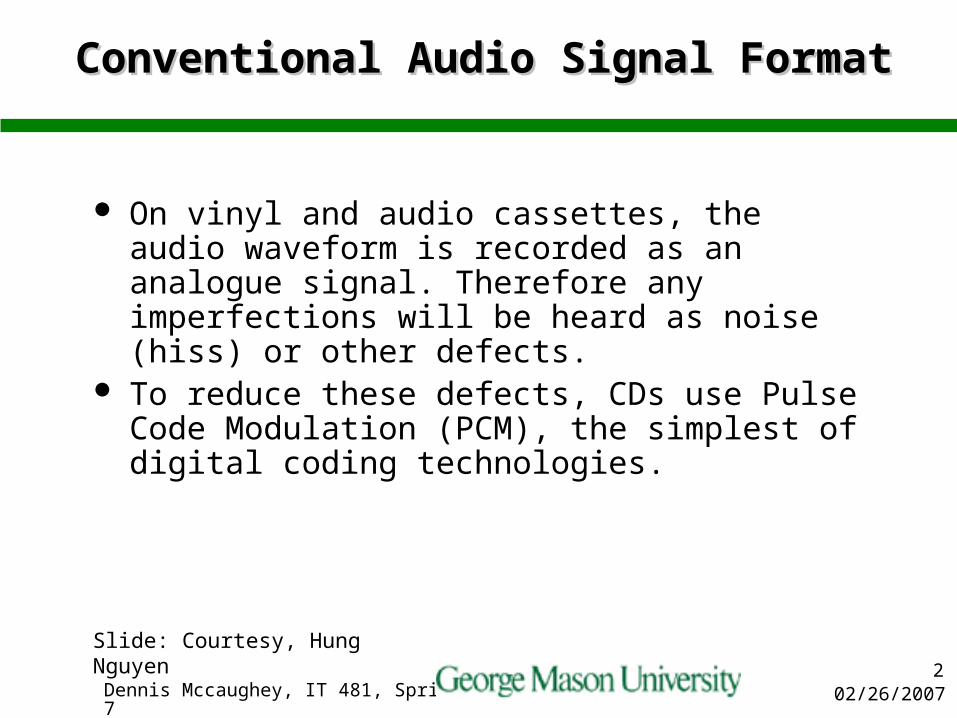
On vinyl and audio cassettes, the audio waveform is recorded as an analogue signal. Therefore any imperfections will be heard as noise (hiss) or other defects.

To reduce these defects, CDs use Pulse Code Modulation (PCM), the simplest of digital coding technologies.

Slide: Courtesy, Hung Nguyen


Pulse Code Modulation (PCM)Pulse Code Modulation (PCM)

Using PCM technology samples of the analogue waveform are taken at intervals and stored as numbers. The example below shows the conversion of an analogue waveform (which could be part of an audio signal) to digital by representing each sample by a number (from 0 to 100 in this simple example).



Sampling for Audio SignalSampling for Audio Signal

In practice the range of values and sampling rate must be high enough to ensure accurate reproduction of the original analogue waveform.

The upper limit for the human ear is about 20kHz therefore the audio must be sampled at 40,000 times per second or higher (since two samples are required for both halves of a sine wave).

To reduce distortion and quantization noise each sample must be represented by at least a 16-bit number giving 65,536 values or levels (0 to 65,535) per sample.



CD Digital Audio ParametersCD Digital Audio Parameters

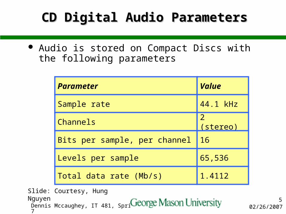
Audio is stored on Compact Discs with the following parameters

Parameter Value

Sample rate 44.1 kHz

Channels 2 (stereo)

Bits per sample, per channel 16

Levels per sample 65,536

Total data rate (Mb/s) 1.4112



Data Integrity in Audio-CDData Integrity in Audio-CD

Digital encoding allows the use of error correction codes, which are necessary to correct errors resulting from the manufacturing process and minor damage or marks which may occur from handling and use.

The result is that the amount of data stored on a CD is nearly four times the data needed to represent the audio only. But this is a small price to pay for a robust format that allows recordings to be played back free of clicks, hiss and other defects associated with analog media.



CD Error Correction and ModulationCD Error Correction and Modulation

Error correction provided by CIRC (Cross Interleaved Read-Solomon Code), which adds two dimensional parity information and also interleaves the data on the disc to protect from burst errors– CIRC corrects error bursts up to 3,500 bits (2.4 mm in length) and

compensates for error bursts up to 12,000 bits (8.5 mm) such as caused by minor scratches.

EFM (Eight to Fourteen) modulation: as CD-ROM discs uses a 14-bit byte, a modification necessary because of the way data is stored and read with lasers, using the pits (indentations) and lands (spaces between indentations) on the disc.– In transferring from magnetic to optical media, the 8-bit byte is

modulated and stored on optical media as a 14-bit byte. This reduces the effect of jitter and other distortions on the error rate.

– When the computer reads the CD-ROM, an interface card demodulates the 14-bit optical code back to 8-bit code.



CD Data FormatCD Data Format



DVD Coding FormatDVD Coding Format

Audio Object Video Object

Encoding methods(mandatory)

Linear PCM(Scalable)Packed PCM (lossless encoding)

Linear PCMDolby AC3

Encoding methods(optional)

none

MPEG AudioDTSSDDS

Audio specifications for Linear PCM and Packed PCM encoding schemes

Sampling frequency 48/96/192 kHz, 44.1/88.2/176.4 kHz 48/96 kHz

Quantization depth 16/20/24 bits 16/20/24 bits

Maximum number of channels

6ch (fs: 48/96/44.1/88.2 kHz) or2ch (fs: 192/176.4 kHz)

8ch(2ch for Stereo

+ 6ch for Multi channel)

Maximum bit rate9.6 Mbps(Linear PCM / Packed

PCM) 6.144 Mbps

(Linear PCM)

Frame rate1200Hz (fs: 48/96/192 kHz)

1102.5Hz (fs: 44.1/88.2/176.4 kHz) 600Hz

(fs: 48/96 kHz)


Dynamic Range of CD and DVDDynamic Range of CD and DVD



Delta ModulationDelta Modulation

In delta modulation, differences between speech samples are encoded & original to be recovered by the decoder at the receiving end

The analog signal is approximated with a series of segments

Each segment of the approximated signal is compared to the original analog wave to determine the increase or decrease in relative amplitude,

The decision process for establishing the state of successive bits is determined by this comparison, and

Only the change of information is sent, i.e., only an increase or decrease of the signal amplitude from the previous sample is sent whereas a no-change condition causes the modulated signal to remain at the same 0 or 1 state of the previous sample.



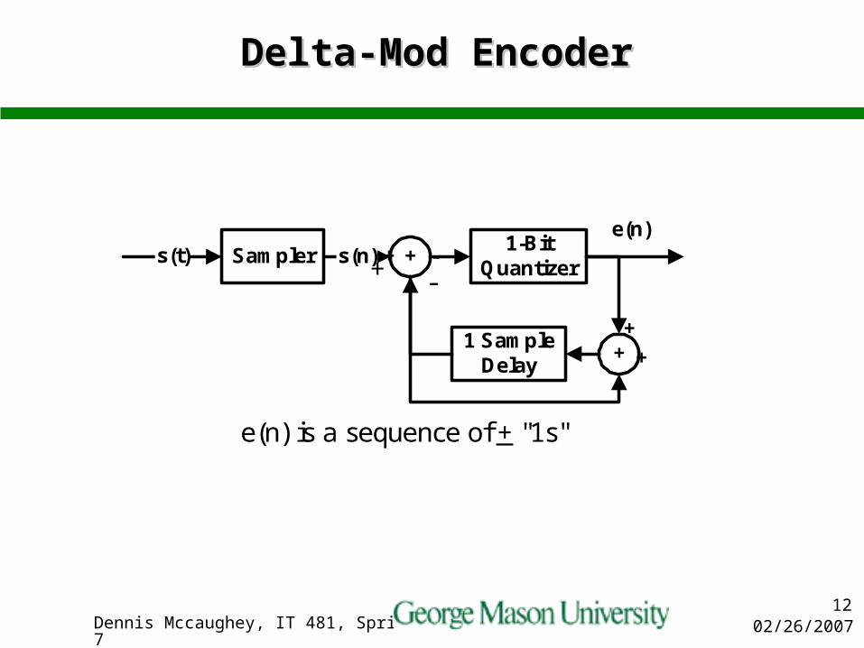
Delta-Mod EncoderDelta-Mod Encoder

1-BitQuantizer

Sampler +

1 SampleDelay

+

s(n)s(t)e(n)

+ -

+

+

e(n) is a sequence of + "1s"

+ -


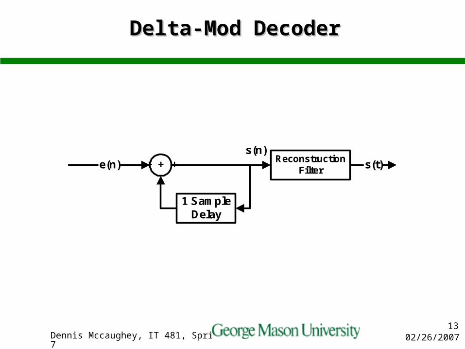
Delta-Mod DecoderDelta-Mod Decoder

ReconstructionFilter+

1 SampleDelay

s(t)e(n) + ++s(n)


Delta Modulation - exampleDelta Modulation - example


Delta Modulation VariantsDelta Modulation Variants

Examples of delta modulation are continuously variable slope delta modulation and delta-sigma modulation.– Continuously variable slope delta (CVSD) modulation:

A type of delta modulation in which the size of the steps of the approximated signal is progressively increased or decreased as required to make the approximated signal closely match the input analog wave.

– Sigma-Delta Modulation: Delta modulation in which the integral of the input signal is encoded rather than the signal itself. Note: Sigma-Delta modulation may be achieved by including a digital integrator preceding the Quantizer in a delta-modulation encoder.

Important concept in “State-of-the-Art” A/D convertersSlide: Courtesy, Hung Nguyen


Sigma-Delta-Mod EncoderSigma-Delta-Mod Encoder

QuantizerSampler +1 Sample

Delay+s(t)

e(n)

+ - +

q(n)+


G.721 Adaptive Differential Pulse Code G.721 Adaptive Differential Pulse Code Modulation (ADPCM)Modulation (ADPCM)

PCM does not attempt to remove speech signal redundancy, this is done by the ADPCM encoder

The CCITT standard G.721 ADPCM algorithm for 32 kbps speech coding used in CT2 and DECT cordless phone systems

In practice, ADPCM encoders are implemented using a linear predictor for the current sample, and the difference between predicted and actual sample (prediction error) is encoded for transmission

Prediction is based on the knowledge of the autocorrelation property of speech



Adaptive PCM ExampleAdaptive PCM Example

In an adaptive PCM system for speech coding, the input signal is sampled at 8 KHz and each sample is represented by 8 bits. The quantizer step size is recomputed every 10 msec and is encoded for transmission using 5 bits. What would the transmission bit rate of such a speech coder?– Sampling frequency = fs = 8 KHz– Number of bits per sample = n = 8 bits– Number of information bits per second = 8,000x8 = 64,000

bits/sec– Quantization step sized recomputed every 10 msec, we

have 100 step size sample to be transmitted every second– Therefore, the number of overhead bits = 100x5 = 500

bits/sec, and the effective transmission bit rate is 64,000+500 = 65,000 bits/sec



ADPCM Encoder used in CT2ADPCM Encoder used in CT2



DPCM Encoder (Simplified)DPCM Encoder (Simplified)

QuantizerSampler Coder+

1 SampleDelay

a

+

s(n)s(t)e(n)

+-

+

+

Neglecting the Quantizer, it is easy to show:

e(n) = s(n) – as(n-1)

The Coder may be a Huffman/Entropy encoder


DPCM Decoder (Simplified)DPCM Decoder (Simplified)

ReconstructionFilter+

1 SampleDelay

a

s(t)e(n) + ++s(n)

Decoder


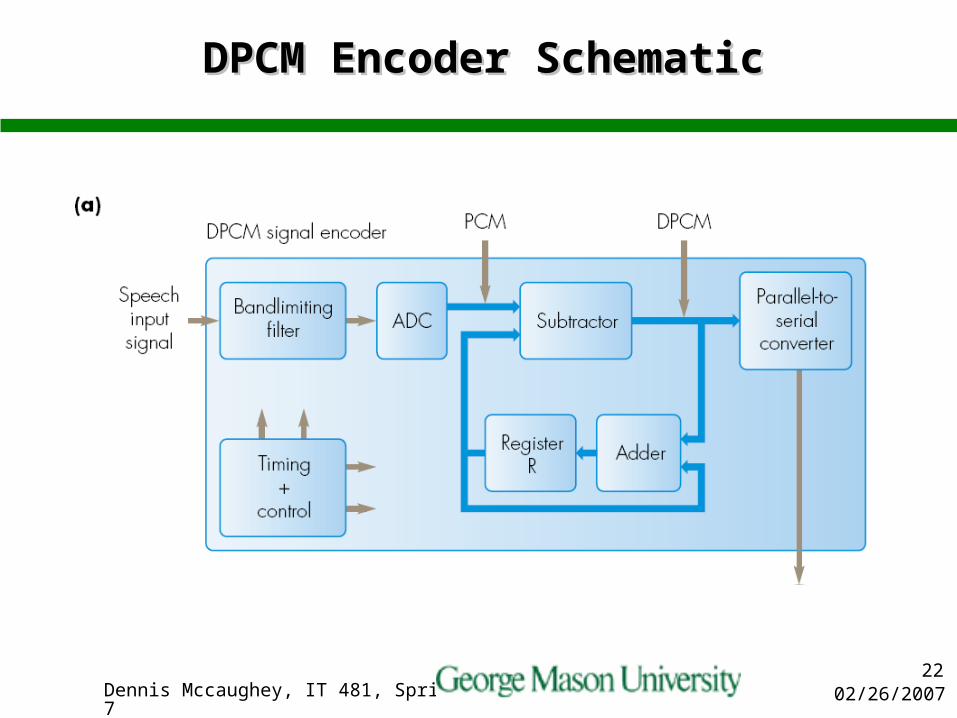
DPCM Encoder SchematicDPCM Encoder Schematic


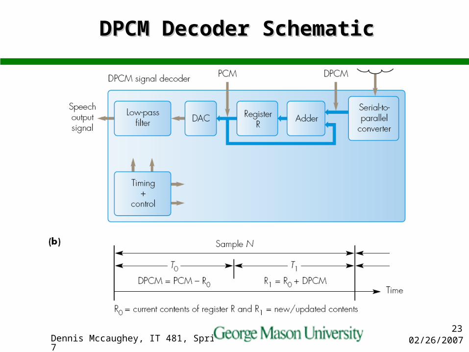
DPCM Decoder SchematicDPCM Decoder Schematic


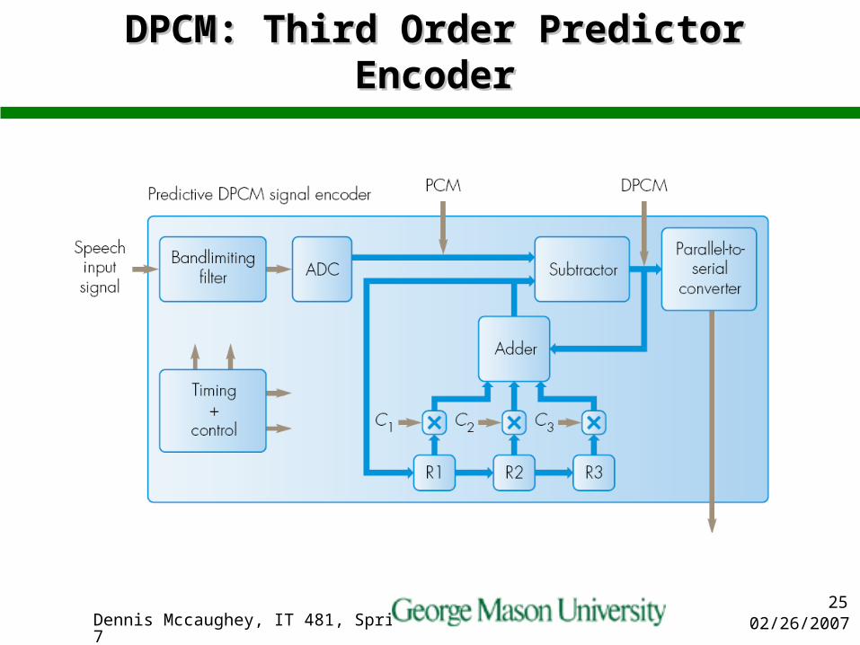
Increased Predictor OrderIncreased Predictor Order

Can improve the compression performance by increasing the number of samples beyond the previous one

In the example a 3rd order predictor is used– The previous three samples contained in R1, R2

&R3 are weighted by C1, C2 &C3 and added to form the overall prediction

– C1, C2 and C3 are functions of the correlation between the first sample and the following two

– e.g. for a Markov Process C2 =(C1)2 C3 = (C1)3


DPCM: Third Order Predictor EncoderDPCM: Third Order Predictor Encoder


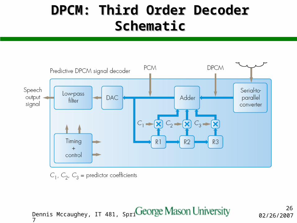
DPCM: Third Order Decoder SchematicDPCM: Third Order Decoder Schematic


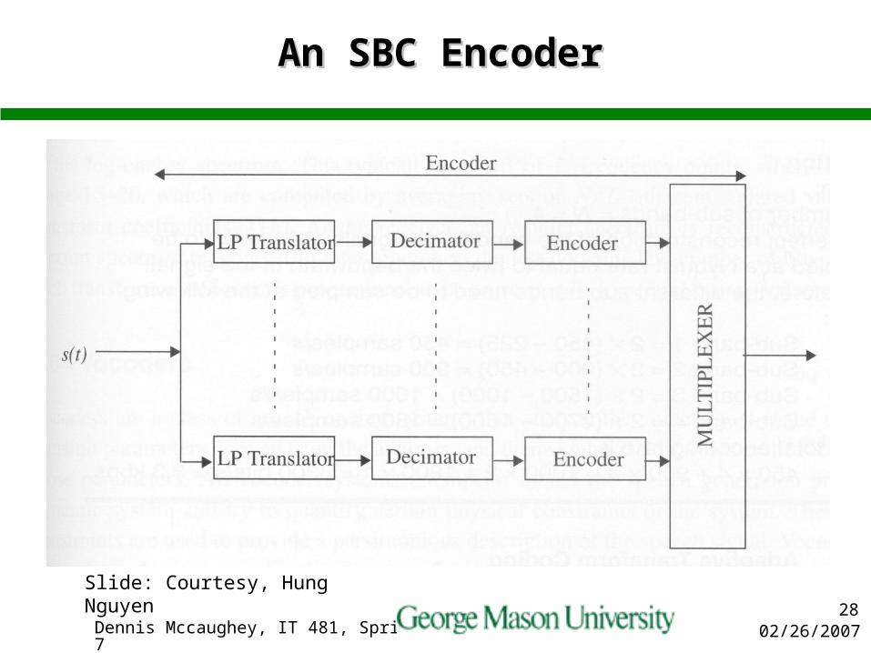
Sub-band Coding (SBC)Sub-band Coding (SBC)

Quantization typically produces distortion broad in spectrum. But human ear does not detect distortion equally well at all frequency

Thus it’s possible to achieve substantial improvement in quality by coding speech in narrower bands

Speech is typically divided into four or eight sub-bands by a bank of filters and each sub-band is sampled at a band-pass Nyquist rate and encoded accordance to a perceptual criteria

SBC can be thought of as a method of controlling and distributing quantization noise across the signal spectrum



An SBC EncoderAn SBC Encoder



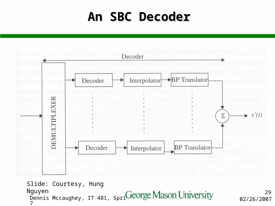
An SBC DecoderAn SBC Decoder



Example of SBCExample of SBC

This table gives the frequency range of each band with the number of bits used to encode each band

Assuming that no side information needs to be transmitted, compute the minimum encoding rate of this SBC encoder

SB Number Frequency (Hz) # of encoded bits

1 225-450 4

2 450-900 3

3 1000-1500 2

4 1800-2700 1



Example of SBC (cont’d)Example of SBC (cont’d)

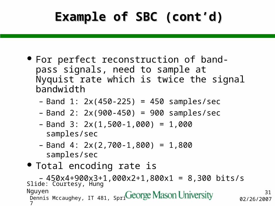
For perfect reconstruction of band-pass signals, need to sample at Nyquist rate which is twice the signal bandwidth– Band 1: 2x(450-225) = 450 samples/sec– Band 2: 2x(900-450) = 900 samples/sec– Band 3: 2x(1,500-1,000) = 1,000 samples/sec– Band 4: 2x(2,700-1,800) = 1,800 samples/sec

Total encoding rate is– 450x4+900x3+1,000x2+1,800x1 = 8,300 bits/s



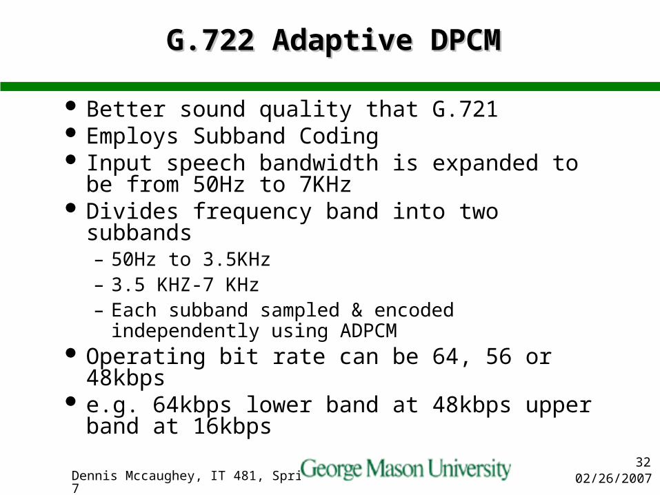
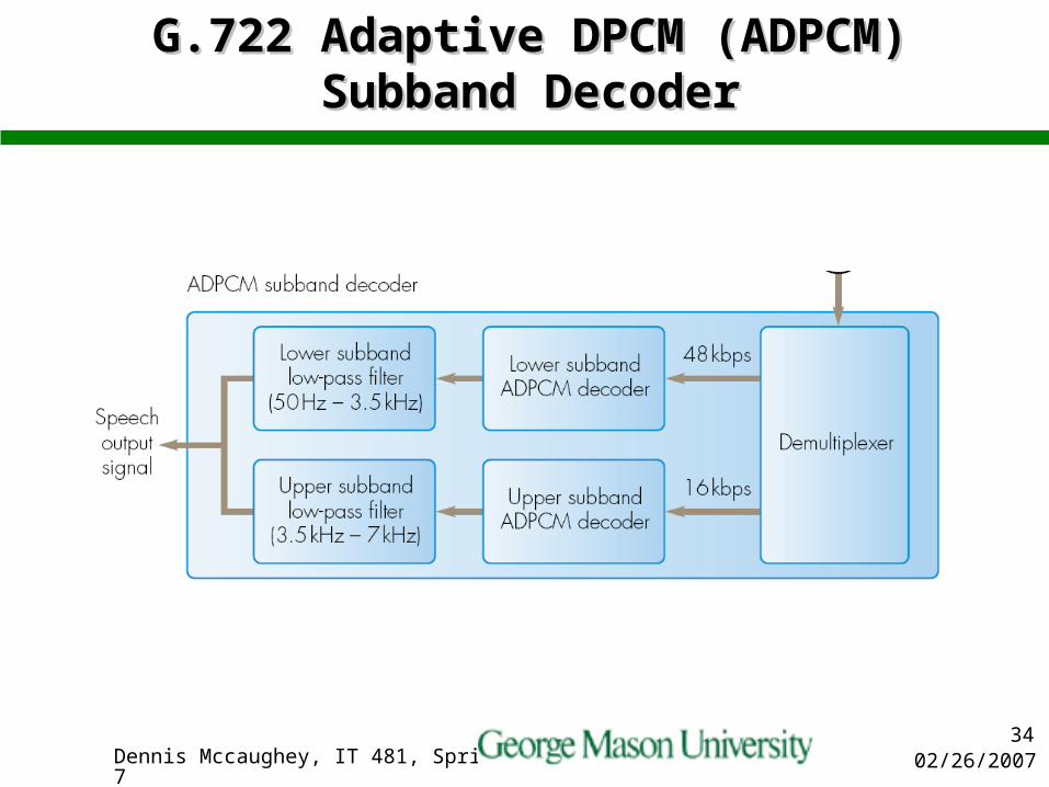
G.722 Adaptive DPCMG.722 Adaptive DPCM

Better sound quality that G.721 Employs Subband Coding Input speech bandwidth is expanded to be

from 50Hz to 7KHz Divides frequency band into two subbands

– 50Hz to 3.5KHz– 3.5 KHZ-7 KHz– Each subband sampled & encoded

independently using ADPCM Operating bit rate can be 64, 56 or 48kbps e.g. 64kbps lower band at 48kbps upper

band at 16kbps


G.722 Adaptive DPCM (ADPCM) G.722 Adaptive DPCM (ADPCM) Subband EncoderSubband Encoder


G.722 Adaptive DPCM (ADPCM) G.722 Adaptive DPCM (ADPCM) Subband DecoderSubband Decoder


Linear Predictive CodingLinear Predictive Coding

LPC analyzes the audio waveform to determine a selection of perceptual features it contains

These are then quantized and sent to the destination together with a sound synthesizer that regenerates the sound that is perceptually comparable with the original

While sounding synthetic very high compression ratios can be obtained


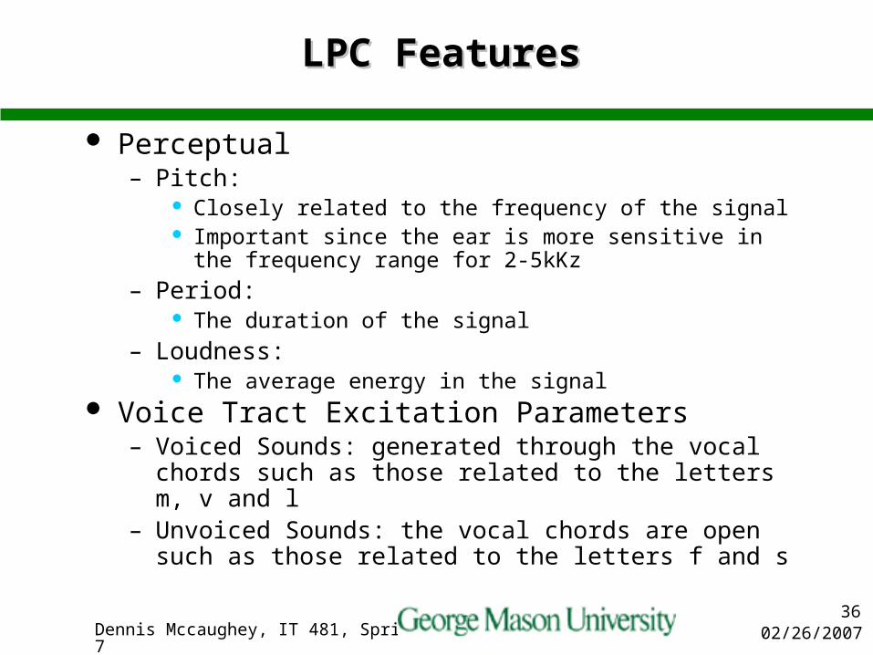
LPC FeaturesLPC Features

Perceptual– Pitch:

Closely related to the frequency of the signal Important since the ear is more sensitive in the frequency

range for 2-5kKz

– Period: The duration of the signal

– Loudness: The average energy in the signal

Voice Tract Excitation Parameters– Voiced Sounds: generated through the vocal chords such

as those related to the letters m, v and l– Unvoiced Sounds: the vocal chords are open such as

those related to the letters f and s


Linear Predictive Coding (LPC) Signal Linear Predictive Coding (LPC) Signal EncoderEncoder


Linear Predictive Coding (LPC) Signal Linear Predictive Coding (LPC) Signal DecoderDecoder


Perceptual Properties of the Ear: Perceptual Properties of the Ear: Sensitivity as a Function of FrequencySensitivity as a Function of Frequency

The ear is most sensitive in the range of 2-5kHzTone A is audible while tone B is not


Perceptual Properties of the Ear: Perceptual Properties of the Ear: Frequency MaskingFrequency Masking

Loud tone suppresses a quieter one. Tone B masks Tone A.Tone B is audible while Tone A is not even if Tone A is audible by itself


Variation with Frequency Effect of Variation with Frequency Effect of Frequency MaskingFrequency Masking

The masking effect is a function of frequency band. The width of each curve at a particular sound level is known as the critical bandwidth. Experiments show the critical bandwidth increases linearly in steps of 100Hz. e.g. for a signal of 1kHz (2x500Hz) the critical bandwidth is about 200Hz


Temporal Masking Caused by a Loud Temporal Masking Caused by a Loud SignalSignal

After the ear hears a loud sound, there is a delay before it can hear a quieter sound


MPEG Perceptual Audio CodingMPEG Perceptual Audio Coding

Perceptual encoding is a lossy compression technique, – i.e. the decoded data is not an exact replica of the original

digital audio data. – Instead, digital audio data is compressed in a way that

despite the high compression rate the decoded audio sounds exactly - or as closely as possible - like the original audio.

This is achieved by adapting the encoding process to the characteristics of the human perception of sound:

The parts of the audio signal that humans perceive distinctly are coded with high accuracy,

The less distinctive parts are coded less accurately, and parts of the sound we do not hear at all are mostly discarded or replaced by quantization noise.


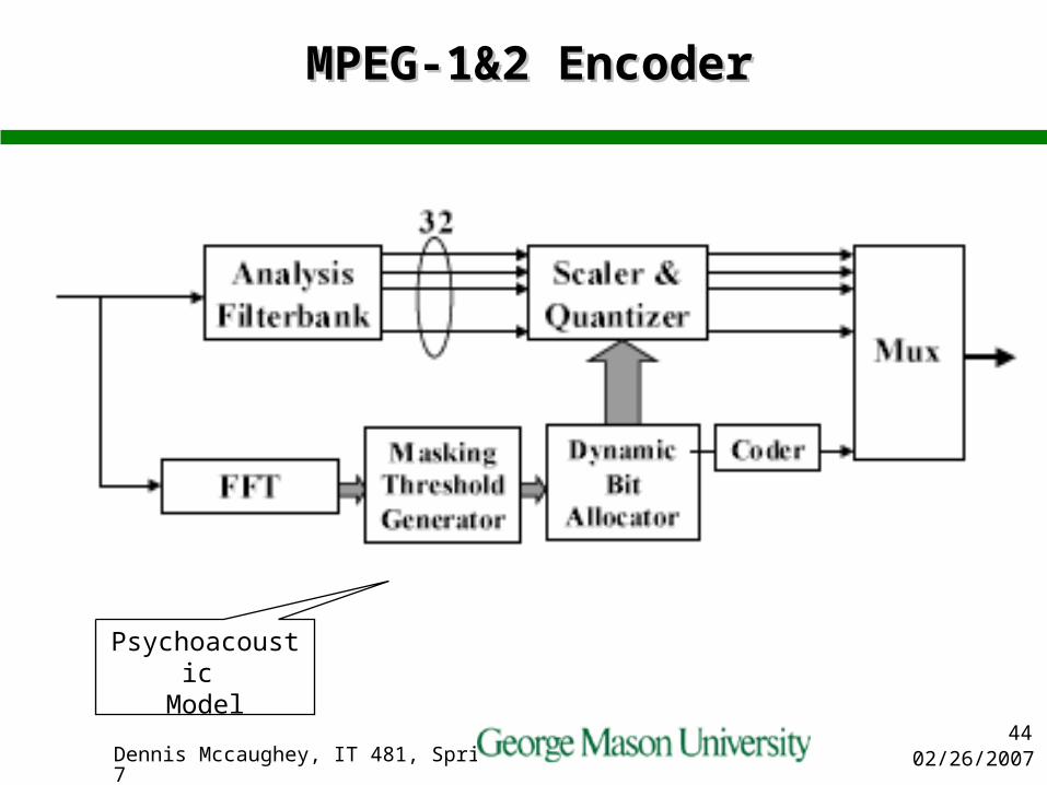
MPEG-1&2 EncoderMPEG-1&2 Encoder

Psychoacoustic Model


New Features for Layer 3 (MP3)New Features for Layer 3 (MP3)

Modified DCT (MDCT)– DCT with overlap– Long/short window switching

Short for better temporal resolution (to prevent pre-echoes)

Long for better frequency resolution

Non-uniform quantization Entropy coding

– Run-length and Huffman coding Bit reservoir (buffer)


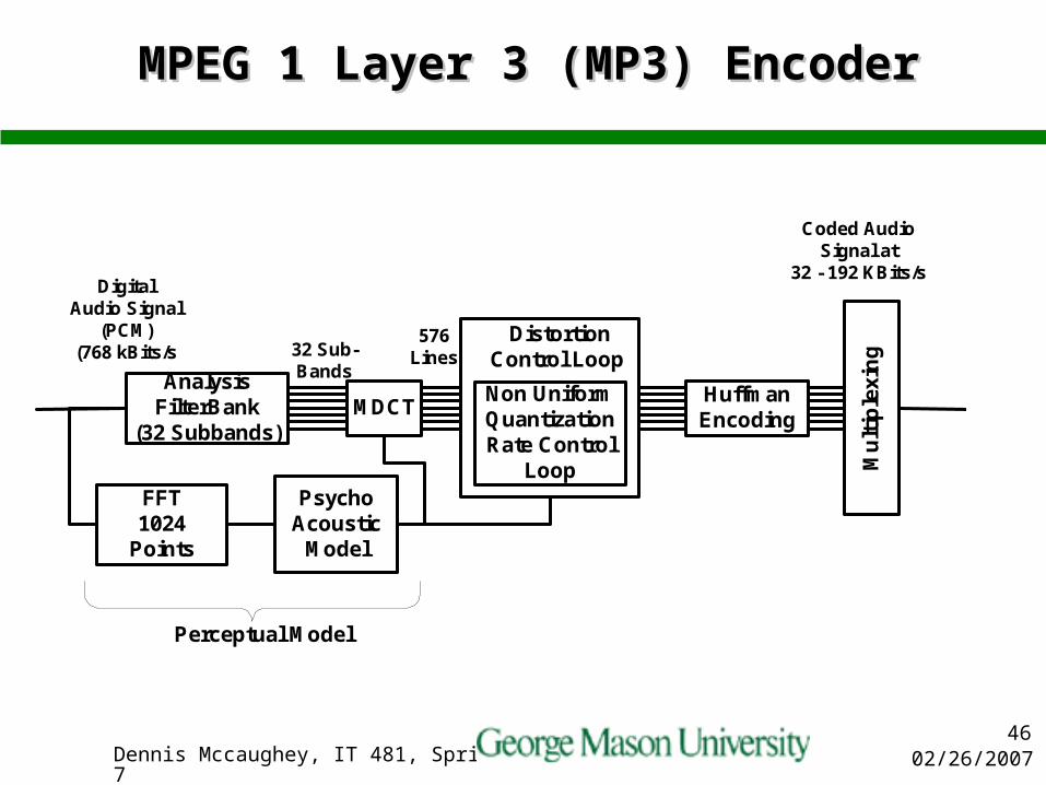
MPEG 1 Layer 3 (MP3) EncoderMPEG 1 Layer 3 (MP3) Encoder

HuffmanEncoding

PsychoAcoustic

Model

FFT1024

Points

Mu

ltip

lexi

ng

AnalysisFilterBank

(32 Subbands)MDCT

32 Sub-Bands

576Lines

DigitalAudio Signal

(PCM)(768 kBits/s

Coded AudioSignal at

32 - 192 KBits/s

Non UniformQuantizationRate Control

Loop

DistortionControl Loop

Perceptual Model


MP3 ComponentsMP3 Components

Perceptual model: An estimate of the actual (time and frequency dependent) masking threshold is computed by using rules known from psychoacoustics.

Filter bank: A hybrid polyphase / MDCT filter bank is used to decompose the input signal into sub-sampled spectral components. Together with the corresponding inverse filter bank in the decoder it forms an analysis/synthesis system.

Quantization and coding: The spectral components are quantized and coded with the aim of keeping the noise introduced by the quantization below the masking threshold.– Distortion Control Loop– Non-uniform Quantization Control Loop– Huffman Coding

Multiplexing: A bit stream formatter is used to assemble the bit stream, which consists of the quantized and coded spectral coefficients and some side information, e.g. bit allocation information.


Perceptual ModelPerceptual Model

The perceptual model consists of outputs values for the masking threshold or allowed noise for each coder partition.

In Layer-3, these coder partitions are roughly equivalent to the critical bands of human hearing. – The the compression result should be

indistinguishable from the original signal If the quantization noise can be kept below the masking threshold for each coder partition


Psychoacoustic ModelPsychoacoustic Model

Time align audio data – The psychoacoustic model must account for both the

delay of the au dio data through the filter bank and a data off-set so that the relevant data is centered within its analysis window

Convert audio to spectral domain– The psychoacoustic model uses a time-to-frequency map-

ping such as a 512- or 1,024-point Fourier transform– A standard Hanning window, applied to audio data before

Fourier transformation, condi tions the data to reduce the edge effects of the transform window.

Partition spectral values into critical bands– To simplify the psychoacoustic calculations, the model

groups the frequency values into perceptual quanta


MPEG Audio Filter Bank BoundariesMPEG Audio Filter Bank Boundaries

Finer resolution at lower frequencies


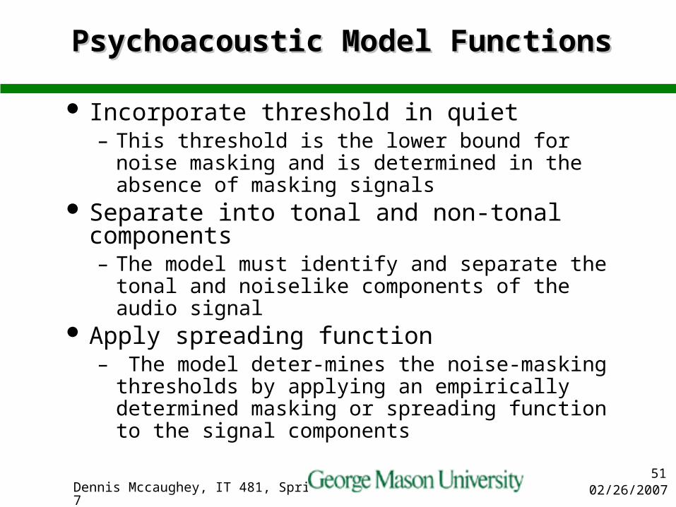
Psychoacoustic Model FunctionsPsychoacoustic Model Functions

Incorporate threshold in quiet– This threshold is the lower bound for noise

masking and is determined in the ab sence of masking signals

Separate into tonal and non-tonal components – The model must identify and separate the tonal

and noiselike components of the audio signal Apply spreading function

– The model deter-mines the noise-masking thresholds by applying an empirically determined masking or spreading function to the signal components


Psychoacoustic Model FunctionsPsychoacoustic Model Functions

Find the minimum masking threshold for each sub-band– The psychoacoustic model calculates the masking

thresholds with a higher-frequency resolution than provided by the filter banks.

– Where the filter band is wide relative to the critical band (at the lower end of the spectrum), the model selects the minimum of the masking thresholds covered by the filter band.

– Where the filter band is narrow relative to the critical band, the model uses the average of the masking thresholds covered by the filter band.


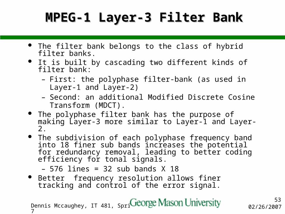
MPEG-1 Layer-3 Filter BankMPEG-1 Layer-3 Filter Bank

The filter bank belongs to the class of hybrid filter banks. It is built by cascading two different kinds of filter bank:

– First: the polyphase filter-bank (as used in Layer-1 and Layer-2)

– Second: an addi tional Modified Discrete Cosine Transform (MDCT).

The polyphase filter bank has the purpose of making Layer-3 more similar to Layer-1 and Layer-2.

The subdivision of each polyphase frequency band into 18 finer sub bands increases the potential for redundancy removal, leading to better coding efficiency for tonal signals. – 576 lines = 32 sub bands X 18

Better frequency resolution allows finer tracking and control of the error signal.


Inner Non-uniform Quantization Rate Control LoopInner Non-uniform Quantization Rate Control Loop

The Huffman code tables assign shorter code words to (more frequent) smaller quantized values.

If the number of bits exceeds the number of bits available to code a given block of data, the global gain adjusted result larger quantization step sizes, thus smaller quantized values.

This operation is repeated with different quantization step sizes until the resulting bit demand for Huffman coding is small enough. The loop is called a rate loop because it modifies the overall coder rate until it is small enough


Distortion Control LoopDistortion Control Loop

The quantization noise is shaped according to the masking threshold, scale factors are applied to each scale factor band.

If the quantization noise in a given band is found to exceed the masking threshold (allowed noise) as supplied by the perceptual model, the scale factor for this band is adjusted to reduce the quantization noise.

A smaller quantization noise re-quires a larger number of quantization steps and thus a higher bit-rate.– Thus the Non-uniform Quantization Rate Control Loop is

repeated every time new scale factors are used. The outer Distortion Control Loop is executed until the actual

noise (computed from the difference of the original spectral values minus the quantized spectral values) is below the masking threshold for every scale factor band (i.e. critical band).


Rate Distortion CriteriaRate Distortion Criteria

Shannon’s Rate Distortion Theorem states that there is a mapping from a source waveform to output code words such that for a given distortion D, R(D) bits/sample are sufficient to reconstruct to waveform with an average distortion that is arbitrarily close to D

The function R(D) is called the rate distortion function and represents the fundamental limit on the achievable rate for a given distortion.

Shannon predicted that such theoretical limit cannot be achieved by one sample at a time as in scalar quantizer but rather by coding many samples at a time by vector quantization



Vector Quantization (VQ)Vector Quantization (VQ)

VQ [Gray] is a delayed-decision coding technique which maps a vector of input samples, typically a speech frame, to a code book index.

The code book has a finite set of vectors covering the entire range of input values

In each quantizing interval, the code book is searched for the best match of the input frame.

VQ can yield better performance even when the samples are independent of one another, and performs best when there is strong correlation between samples in the group



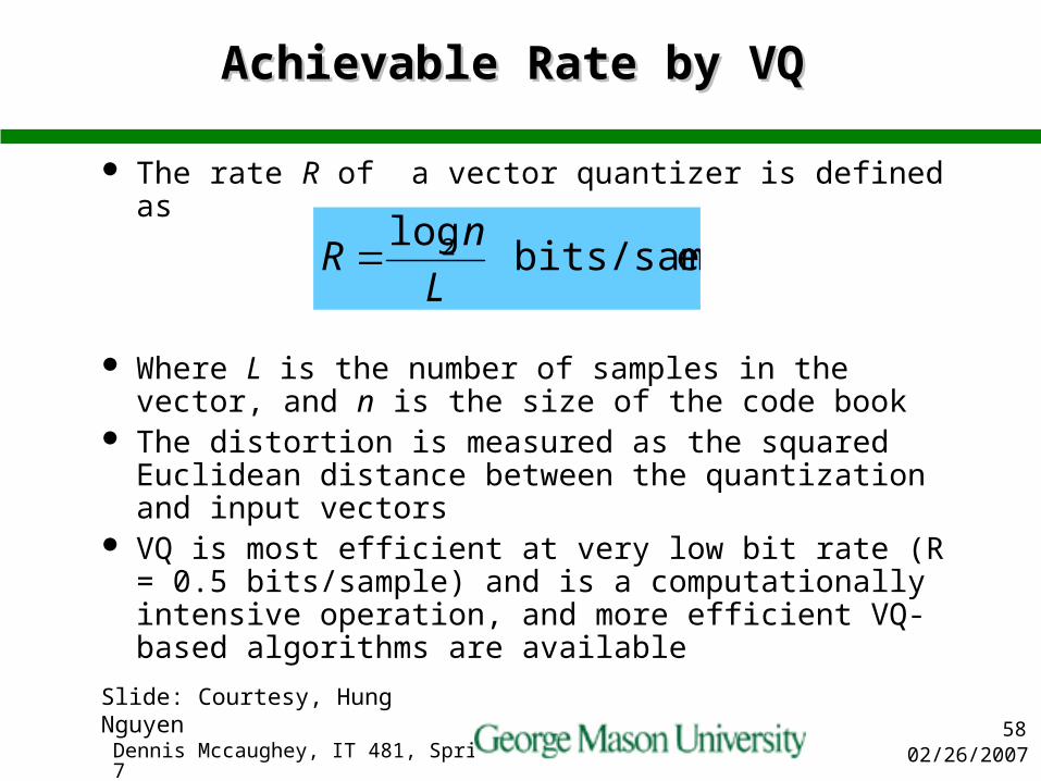
Achievable Rate by VQ Achievable Rate by VQ

The rate R of a vector quantizer is defined as

Where L is the number of samples in the vector, and n is the size of the code book

The distortion is measured as the squared Euclidean distance between the quantization and input vectors

VQ is most efficient at very low bit rate (R = 0.5 bits/sample) and is a computationally intensive operation, and more efficient VQ-based algorithms are available

ebits/sampl log2

L

nR



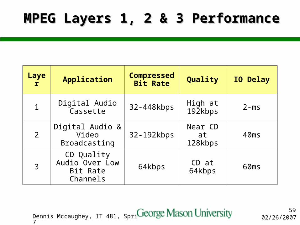
MPEG Layers 1, 2 & 3 PerformanceMPEG Layers 1, 2 & 3 Performance

Layer Application Compressed Bit Rate Quality IO Delay

1 Digital Audio Cassette 32-448kbps High at

192kbps 2-ms

2 Digital Audio & Video Broadcasting 32-192kbps Near CD at

128kbps 40ms

3CD Quality Audio Over Low Bit Rate

Channels64kbps CD at

64kbps 60ms


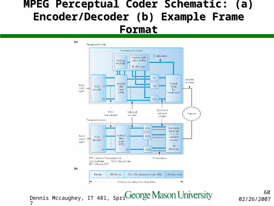
MPEG Perceptual Coder Schematic: (a) MPEG Perceptual Coder Schematic: (a) Encoder/Decoder (b) Example Frame FormatEncoder/Decoder (b) Example Frame Format


Perceptual Coder Schematics: (a) Forward Adaptive Bit Perceptual Coder Schematics: (a) Forward Adaptive Bit Allocation (MPEG); (b) Fixed Bit Allocation (Dolby AC-1)Allocation (MPEG); (b) Fixed Bit Allocation (Dolby AC-1)


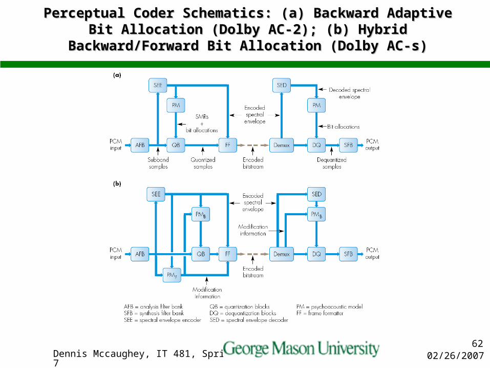
Perceptual Coder Schematics: (a) Backward Adaptive Bit Perceptual Coder Schematics: (a) Backward Adaptive Bit Allocation (Dolby AC-2); (b) Hybrid Backward/Forward Bit Allocation (Dolby AC-2); (b) Hybrid Backward/Forward Bit

Allocation (Dolby AC-s)Allocation (Dolby AC-s)


Mid Term TopicsMid Term Topics

Huffman Code Advantages of digital over analog audio Shannon’s Sampling Theorem IIR and FIR digital filters Quality of Service JPEG compression process What is multimedia Why are psychoacoustics important DPCM and how it works (fundamental

principle) User and network requirements

concepts of multimedia processing and transmission it 481, lecture 6 dennis mccaughey, ph.d. 26...

Documents

nguyendennis mccaughey

audio waveform

audio cassettes

audio signalin

cd error correction

optical code

cd data formatslide

error bursts