concentration inequalities
DESCRIPTION
SurveyTRANSCRIPT

Concentration Inequalities
Stephane Boucheron1, Gabor Lugosi2, and Olivier Bousquet3
1 Universite de Paris-Sud, Laboratoire d’InformatiqueBatiment 490, F-91405 Orsay Cedex, France
WWW home page: http://www.lri.fr/~bouchero2 Department of Economics, Pompeu Fabra University
Ramon Trias Fargas 25-27, 08005 Barcelona, [email protected]
WWW home page: http://www.econ.upf.es/~lugosi3 Max-Planck Institute for Biological Cybernetics
Spemannstr. 38, D-72076 Tubingen, [email protected]
WWW home page: http://www.kyb.mpg.de/~bousquet
Abstract. Concentration inequalities deal with deviations of functionsof independent random variables from their expectation. In the lastdecade new tools have been introduced making it possible to establishsimple and powerful inequalities. These inequalities are at the heart ofthe mathematical analysis of various problems in machine learning andmade it possible to derive new efficient algorithms. This text attemptsto summarize some of the basic tools.
1 Introduction
The laws of large numbers of classical probability theory state that sums ofindependent random variables are, under very mild conditions, close to theirexpectation with a large probability. Such sums are the most basic examplesof random variables concentrated around their mean. More recent results revealthat such a behavior is shared by a large class of general functions of independentrandom variables. The purpose of these notes is to give an introduction to someof these general concentration inequalities.
The inequalities discussed in these notes bound tail probabilities of generalfunctions of independent random variables. Several methods have been known toprove such inequalities, including martingale methods (see Milman and Schecht-man [1] and the surveys of McDiarmid [2, 3]), information-theoretic methods (seeAlhswede, Gacs, and Korner [4], Marton [5, 6, 7], Dembo [8], Massart [9] and Rio[10]), Talagrand’s induction method [11, 12, 13] (see also Luczak and McDiarmid[14], McDiarmid [15] and Panchenko [16, 17, 18]), the decoupling method sur-veyed by de la Pena and Gine [19], and the so-called “entropy method”, based onlogarithmic Sobolev inequalities, developed by Ledoux [20, 21], see also Bobkov
216 Stephane Boucheron, Gabor Lugosi, and Olivier Bousquet
and Ledoux [22], Massart [23], Rio [10], Klein [24], Boucheron, Lugosi, and Mas-sart [25, 26], Bousquet [27, 28], and Boucheron, Bousquet, Lugosi, and Massart[29]. Also, various problem-specific methods have been worked out in randomgraph theory, see Janson, Luczak, and Rucinski [30] for a survey.
First of all we recall some of the essential basic tools needed in the rest ofthese notes. For any nonnegative random variable X,
�X =
∫ ∞
0
� {X ≥ t}dt .
This implies Markov’s inequality: for any nonnegative random variable X, andt > 0,
� {X ≥ t} ≤�X
t.
If follows from Markov’s inequality that if φ is a strictly monotonically increasingnonnegative-valued function then for any random variable X and real number t,
� {X ≥ t} =� {φ(X) ≥ φ(t)} ≤
�φ(X)
φ(t).
An application of this with φ(x) = x2 is Chebyshev’s inequality: if X is anarbitrary random variable and t > 0, then
� {|X − �X| ≥ t} =
� {|X − �X|2 ≥ t2
}≤
� [|X − �X|2
]
t2=
Var{X}t2
.
More generally taking φ(x) = xq (x ≥ 0), for any q > 0 we have
� {|X − �X| ≥ t} ≤
�[|X − �
X|q]tq
.
In specific examples one may choose the value of q to optimize the obtainedupper bound. Such moment bounds often provide with very sharp estimatesof the tail probabilities. A related idea is at the basis of Chernoff’s bounding
method. Taking φ(x) = esx where s is an arbitrary positive number, for anyrandom variable X, and any t > 0, we have
� {X ≥ t} =� {esX ≥ est} ≤
�esX
est.
In Chernoff’s method, we find an s > 0 that minimizes the upper bound ormakes the upper bound small.
Next we recall some simple inequalities for sums of independent random vari-ables. Here we are primarily concerned with upper bounds for the probabilitiesof deviations from the mean, that is, to obtain inequalities for
� {Sn−�Sn ≥ t},
with Sn =∑ni=1Xi, where X1, . . . , Xn are independent real-valued random vari-
ables.Chebyshev’s inequality and independence immediately imply
� {|Sn −�Sn| ≥ t} ≤
Var{Sn}t2
=
∑ni=1 Var{Xi}
t2.

Concentration Inequalities 217
In other words, writing σ2 = 1n
∑ni=1 Var{Xi},
�
{∣∣∣∣∣1
n
n∑
i=1
Xi −�Xi
∣∣∣∣∣ ≥ ε}≤ σ2
nε2.
Chernoff’s bounding method is especially convenient for bounding tail prob-abilities of sums of independent random variables. The reason is that since theexpected value of a product of independent random variables equals the productof the expected values, Chernoff’s bound becomes
� {Sn −�Sn ≥ t} ≤ e−st
�
[exp
(s
n∑
i=1
(Xi −�Xi)
)]
= e−stn∏
i=1
�[es(Xi− � Xi)
](by independence). (1)
Now the problem of finding tight bounds comes down to finding a good upperbound for the moment generating function of the random variables Xi −
�Xi.
There are many ways of doing this. For bounded random variables perhaps themost elegant version is due to Hoeffding [31] which we state without proof.
Lemma 1. hoeffding’s inequality. Let X be a random variable with�X =
0, a ≤ X ≤ b. Then for s > 0,
� [esX
]≤ es2(b−a)2/8.
This lemma, combined with (1) immediately implies Hoeffding’s tail inequal-ity [31]:
Theorem 1. Let X1, . . . , Xn be independent bounded random variables suchthat Xi falls in the interval [ai, bi] with probability one. Then for any t > 0we have
� {Sn −�Sn ≥ t} ≤ e−2t2/
Pni=1(bi−ai)
2
and� {Sn −
�Sn ≤ −t} ≤ e−2t2/
Pni=1(bi−ai)
2
.
The theorem above is generally known as Hoeffding’s inequality. For binomialrandom variables it was proved by Chernoff [32] and Okamoto [33].
A disadvantage of Hoeffding’s inequality is that it ignores information aboutthe variance of the Xi’s. The inequalities discussed next provide an improvementin this respect.
Assume now without loss of generality that�Xi = 0 for all i = 1, . . . , n. Our
starting point is again (1), that is, we need bounds for� [
esXi]. Introduce the
notation σ2i =
�[X2
i ], and
Fi =�
[ψ(sXi)] =
∞∑
r=2
sr−2 �[Xr
i ]
r!σ2i
.
218 Stephane Boucheron, Gabor Lugosi, and Olivier Bousquet
Also, let ψ(x) = exp(x) − x − 1, and observe that ψ(x) ≤ x2/2 for x ≤ 0 andψ(sx) ≤ x2ψ(s) for s ≥ 0 and x ∈ [0, 1]. Since esx = 1 + sx + ψ(sx), we maywrite
� [esXi
]= 1 + s
�[Xi] +
�[ψ(sXi)]
= 1 +�
[ψ(sXi)] (since�
[Xi] = 0.)
≤ 1 +�
[ψ(s(Xi)+) + ψ(−s(Xi)−)]
(where x+ = max(0, x) and x− = max(0,−x))
≤ 1 +�
[ψ(s(Xi)+) +s2
2(Xi)
2−] (using ψ(x) ≤ x2/2 for x ≤ 0. ) .
Now assume that the Xi’s are bounded such that Xi ≤ 1. Thus, we have obtained
� [esXi
]≤ 1 +
�[ψ(s)(Xi)
2+ +
s2
2(Xi)
2−] ≤ 1 + ψ(s)
�[X2
i ] ≤ exp(ψ(s)
�[X2
i ])
Returning to (1) and using the notation σ2 = (1/n)∑σ2i , we get
�
{n∑
i=1
Xi > t
}≤ enσ2ψ(s)−st.
Now we are free to choose s. The upper bound is minimized for
s = log
(1 +
t
nσ2
).
Resubstituting this value, we obtain Bennett’s inequality [34]:
Theorem 2. bennett’s inequality. Let X1, . . ., Xn be independent real-valuedrandom variables with zero mean, and assume that Xi ≤ 1 with probability one.Let
σ2 =1
n
n∑
i=1
Var{Xi}.
Then for any t > 0,
�
{n∑
i=1
Xi > t
}≤ exp
(−nσ2h
(t
nσ2
)).
where h(u) = (1 + u) log(1 + u)− u for u ≥ 0.
The message of this inequality is perhaps best seen if we do some furtherbounding. Applying the elementary inequality h(u) ≥ u2/(2 + 2u/3), u ≥ 0(which may be seen by comparing the derivatives of both sides) we obtain aclassical inequality of Bernstein [35]:

Concentration Inequalities 219
Theorem 3. bernstein’s inequality. Under the conditions of the previoustheorem, for any ε > 0,
�
{1
n
n∑
i=1
Xi > ε
}≤ exp
(− nε2
2(σ2 + ε/3)
).
Bernstein’s inequality points out an interesting phenomenon: if σ2 < ε,then the upper bound behaves like e−nε instead of the e−nε
2
guaranteed byHoeffding’s inequality. This might be intuitively explained by recalling that aBinomial(n, λ/n) distribution can be approximated, for large n, by a Poisson(λ)distribution, whose tail decreases as e−λ.
2 The Efron-Stein Inequality
The main purpose of these notes is to show how many of the tail inequalities forsums of independent random variables can be extended to general functions ofindependent random variables. The simplest, yet surprisingly powerful inequalityof this kind is known as the Efron-Stein inequality. It bounds the variance ofa general function. To obtain tail inequalities, one may simply use Chebyshev’sinequality.
Let X be some set, and let g : X n → �be a measurable function of n
variables. We derive inequalities for the difference between the random variableZ = g(X1, . . . , Xn) and its expected value
�Z when X1, . . . , Xn are arbitrary
independent (not necessarily identically distributed!) random variables takingvalues in X .
The main inequalities of this section follow from the next simple result. Tosimplify notation, we write
�i for the expected value with respect to the variable
Xi, that is,�iZ =
�[Z|X1, . . . , Xi−1, Xi+1, . . . , Xn].
Theorem 4.
Var(Z) ≤n∑
i=1
�[(Z − �
iZ)2].
Proof. The proof is based on elementary properties of conditional expectation.Recall that if X and Y are arbitrary bounded random variables, then
�[XY ] =
�[
�[XY |Y ]] =
�[Y
�[X|Y ]].
Introduce the notation V = Z − �Z, and define
Vi =�
[Z|X1, . . . , Xi]−�
[Z|X1, . . . , Xi−1], i = 1, . . . , n.
220 Stephane Boucheron, Gabor Lugosi, and Olivier Bousquet
Clearly, V =∑ni=1 Vi. (Thus, V is written as a sum of martingale differences.)
Then
Var(Z) =�
(
n∑
i=1
Vi
)2
=�
n∑
i=1
V 2i + 2
� ∑
i>j
ViVj
=�
n∑
i=1
V 2i ,
since, for any i > j,
�ViVj =
� �[ViVj |X1, . . . , Xj ] =
�[Vj
�[Vi|X1, . . . , Xj ]] = 0 .
To bound�V 2i , note that, by Jensen’s inequality,
V 2i = (
�[Z|X1, . . . , Xi]−
�[Z|X1, . . . , Xi−1])
2
=(
�[
�[Z|X1, . . . , Xn]− �
[Z|X1, . . . , Xi−1, Xi+1, . . . , Xn]∣∣∣X1, . . . , Xi
])2
≤ �[(
�[Z|X1, . . . , Xn]− �
[Z|X1, . . . , Xi−1, Xi+1, . . . , Xn])2∣∣∣X1, . . . , Xi
]
=�[(Z − �
iZ)2∣∣∣X1, . . . , Xi
].
Taking expected values on both sides, we obtain the statement. �
Now the Efron-Stein inequality follows easily. To state the theorem, letX ′
1, . . . , X′n form an independent copy of X1, . . . , Xn and write
Z ′i = g(X1, . . . , X
′i, . . . , Xn) .
Theorem 5. efron-stein inequality (efron and stein [36], steele [37]).
Var(Z) ≤ 1
2
n∑
i=1
� [(Z − Z ′
i)2]
Proof. The statement follows by Theorem 4 simply by using (conditionally)the elementary fact that if X and Y are independent and identically distributedrandom variables, then Var(X) = (1/2)
�[(X − Y )2], and therefore
�i
[(Z − �
iZ)2]
=1
2
�i
[(Z − Z ′
i)2]. �
Remark. Observe that in the case when Z =∑ni=1Xi is a sum of independent
random variables (of finite variance) then the inequality in Theorem 5 becomes

Concentration Inequalities 221
an equality. Thus, the bound in the Efron-Stein inequality is, in a sense, notimprovable. This example also shows that, among all functions of independentrandom variables, sums, in some sense, are the least concentrated. Below we willsee other evidences for this extremal property of sums.
Another useful corollary of Theorem 4 is obtained by recalling that, for anyrandom variable X, Var(X) ≤ �
[(X − a)2] for any constant a ∈ �. Using this
fact conditionally, we have, for every i = 1, . . . , n,
�i
[(Z − �
iZ)2]≤ �
i
[(Z − Zi)2
]
where Zi = gi(X1, . . . , Xi−1, Xi+1, . . . , Xn) for arbitrary measurable functionsgi : Xn−1 → �
of n− 1 variables. Taking expected values and using Theorem 4we have the following.
Theorem 6.
Var(Z) ≤n∑
i=1
� [(Z − Zi)2
].
In the next two sections we specialize the Efron-Stein inequality and its vari-ant Theorem 6 to functions which satisfy some simple easy-to-verify properties.
2.1 Functions with Bounded Differences
We say that a function g : X n → �has the bounded differences property if for
some nonnegative constants c1, . . . , cn,
supx1,...,xn,x′
i∈X
|g(x1, . . . , xn)− g(x1, . . . , xi−1, x′i, xi+1, . . . , xn)| ≤ ci , 1 ≤ i ≤ n .
In other words, if we change the i-th variable of g while keeping all the othersfixed, the value of the function cannot change by more than ci. Then the Efron-Stein inequality implies the following:
Corollary 1. If g has the bounded differences property with constants c1, . . . , cn,then
Var(Z) ≤ 1
2
n∑
i=1
c2i .
Next we list some interesting applications of this corollary. In all cases thebound for the variance is obtained effortlessly, while a direct estimation of thevariance may be quite involved.
Example. uniform deviations. One of the central quantities of statisticallearning theory and empirical process theory is the following: let X1, . . . , Xn bei.i.d. random variables taking their values in some set X , and let A be a collection

222 Stephane Boucheron, Gabor Lugosi, and Olivier Bousquet
of subsets of X . Let µ denote the distribution of X1, that is, µ(A) =� {X1 ∈ A},
and let µn denote the empirical distribution:
µn(A) =1
n
n∑
i=1
�
{Xn∈A} .
The quantity of interest is
Z = supA∈A|µn(A)− µ(A)|.
If limn→∞�Z = 0 for every distribution of the Xi’s, then A is called a uni-
form Glivenko-Cantelli class, and Vapnik and Chervonenkis [38] gave a beautifulcombinatorial characterization of such classes. But regardless of what A is, bychanging one Xi, Z can change by at most 1/n, so regardless of the behavior of
�Z, we always have
Var(Z) ≤ 1
2n.
For more information on the behavior of Z and its role in learning theory see,for example, Devroye, Gyorfi, and Lugosi [39], Vapnik [40], van der Vaart andWellner [41], Dudley [42].
Next we show how a closer look at the the Efron-Stein inequality implies asignificantly better bound for the variance of Z. We do this in a slightly moregeneral framework of empirical processes. Let F be a class of real-valued func-tions and define Z = g(X1, . . . , Xn) = supf∈F
∑nj=1 f(Xj). Assume that the
functions f ∈ F are such that�
[f(Xi)] = 0 and take values in [−1, 1]. Let Zibe defined as
Zi = supf∈F
∑
j 6=if(Xj) .
Let f be the function achieving the supremum4 in the definition of Z, that isZ =
∑ni=1 f(Xi) and similarly fi be such that Zi =
∑j 6=i fi(Xj). We have
fi(Xi) ≤ Z − Zi ≤ f(Xi) ,
and thus∑ni=1 Z − Zi ≤ Z. As fi and Xi are independent,
�i[fi(Xi)] = 0. On
the other hand,
(Z − Zi)2 − f2i (Xi) = (Z − Zi + fi(Xi))(Z − Zi − fi(Xi))
≤ 2(Z − Zi + fi(Xi)) .
Summing over all i and taking expectations,
�
[n∑
i=1
(Z − Zi)2]≤ �
[n∑
i=1
f2i (Xi) + 2(Z − Zi) + 2fi(Xi)
]
≤ n supf∈F
�[f2(X1)] + 2
�[Z]
4 If the supremum is not attained the proof can be modified to yield the same result.We omit the details here.

Concentration Inequalities 223
where at the last step we used the facts that�
[fi(Xi)2] ≤ supf∈F
�[f2(X1)],∑n
i=1(Z − Zi) ≤ Z, and�fi(Xi) = 0. Thus, by the Efron-Stein inequality
Var(Z) ≤ n supf∈F
�[f2(X1)] + 2
�[Z]
¿From just the bounded differences property we derived Var(Z) ≤ 2n. Thenew bound may be a significant improvement whenever the maximum of
�f(Xi)
2
over f ∈ F is small. (Note that if the class F is not too large,�Z is typically of
the order of√n.) The exponential tail inequality due to Talagrand [12] extends
this variance inequality, and is one of the most important recent results of thetheory of empirical processes, see also Ledoux [20], Massart [23], Rio [10], Klein[24], and Bousquet [27, 28].
Example. minimum of the empirical loss. Concentration inequalities havebeen used as a key tool in recent developments of model selection methods instatistical learning theory. For the background we refer to the the recent work ofKoltchinskii and Panchenko [43], Massart [44], Bartlett, Boucheron, and Lugosi[45], Lugosi and Wegkamp [46], Bousquet [47].
Let F denote a class of {0, 1}-valued functions on some space X . For sim-plicity of the exposition we assume that F is finite. The results remain true forgeneral classes as long as the measurability issues are taken care of. Given ani.i.d. sample Dn = (〈Xi, Yi〉)i≤n of n pairs of random variables 〈Xi, Yi〉 takingvalues in X × {0, 1}, for each f ∈ F we define the empirical loss
Ln(f) =1
n
n∑
i=1
`(f(Xi), Yi)
where the loss function ` is defined on {0, 1}2 by
`(y, y′) =�y 6=y′ .
In nonparametric classification and learning theory it is common to select anelement of F by minimizing the empirical loss. The quantity of interest in thissection is the minimal empirical loss
L = inff∈F
Ln(f).
Corollary 1 immediately implies that Var(L) ≤ 1/(2n). However, a more care-
ful application of the Efron-Stein inequality reveals that L may be much moreconcentrated than predicted by this simple inequality. Getting tight results forthe fluctuations of L provides better insight into the calibration of penalties incertain model selection methods.
Let Z = nL and let Z ′i be defined as in Theorem 5, that is,
Z ′i = min
f∈F
∑
j 6=i`(f(Xj), Yj) + `(f(Xi
′), Yi′)
224 Stephane Boucheron, Gabor Lugosi, and Olivier Bousquet
where 〈Xi′, Yi
′〉 is independent of Dn and has the same distribution as 〈Xi, Yi〉.Now the convenient form of the Efron-Stein inequality is the following:
Var(Z) ≤ 1
2
n∑
i=1
� [(Z − Z ′
i)2]
=
n∑
i=1
� [(Z − Z ′
i)2 �
Z′i>Z
]
Let f∗ denote a (possibly non-unique) minimizer of the empirical risk so thatZ =
∑nj=1 `(f
∗(Xj), Yj). The key observation is that
(Z − Z ′i)
2 �
Z′i>Z≤ (`(f∗(Xi
′), Yi′)− `(f∗(Xi), Yi))
2 �
Z′i>Z
= `(f∗(X ′i), Y
′i )
�
`(f∗(Xi),Yi)=0 .
Thus,
n∑
i=1
� [(Z − Z ′
i)2 �
Z′i>Z
]≤ � ∑
i:`(f∗(Xi),Yi)=0
�
X′i,Y
′i[`(f∗(X ′
i), Y′i )] ≤ n �
L(f∗)
where�
X′i,Y
′i
denotes expectation with respect to the variables X ′i, Y
′i and for
each f ∈ F , L(f) =�`(f(X), Y ) is the true (expected) loss of f . Therefore, the
Efron-Stein inequality implies that
Var(L) ≤�L(f∗)
n.
This is a significant improvement over the bound 1/(2n) whenever�L(f ∗) is
much smaller than 1/2. This is very often the case. For example, we have
L(f∗) = L− (Ln(f∗)− L(f∗)) ≤ Z
n+ supf∈F
(L(f)− Ln(f))
so that we obtain
Var(L) ≤�L
n+
�supf∈F (L(f)− Ln(f))
n.
In most cases of interest,�
supf∈F (L(f)−Ln(f)) may be bounded by a constant
(depending on F) times n−1/2 (see, e.g., Lugosi [48]) and then the second termon the right-hand side is of the order of n−3/2. For exponential concentrationinequalities for L we refer to Boucheron, Lugosi, and Massart [26].
Example. kernel density estimation. Let X1, . . . , Xn be i.i.d. samplesdrawn according to some (unknown) density f on the real line. The density isestimated by the kernel estimate
fn(x) =1
nh
n∑
i=1
K
(x−Xi
h
),

Concentration Inequalities 225
where h > 0 is a smoothing parameter, and K is a nonnegative function with∫K = 1. The performance of the estimate is measured by the L1 error
Z = g(X1, . . . , Xn) =
∫|f(x)− fn(x)|dx.
It is easy to see that
|g(x1, . . . , xn)− g(x1, . . . , x′i, . . . , xn)| ≤ 1
nh
∫ ∣∣∣∣K(x− xih
)−K
(x− x′ih
)∣∣∣∣ dx
≤ 2
n,
so without further work we get
Var(Z) ≤ 2
n.
It is known that for every f ,√n
�g → ∞ (see Devroye and Gyorfi [49]) which
implies, by Chebyshev’s inequality, that for every ε > 0
�{∣∣∣∣
Z�Z− 1
∣∣∣∣ ≥ ε}
=� {|Z − �
Z| ≥ ε �Z} ≤ Var(Z)
ε2(�Z)2→ 0
as n→∞. That is, Z/�Z → 0 in probability, or in other words, Z is relatively
stable. This means that the random L1-error behaves like its expected value.This result is due to Devroye [50], [51]. For more on the behavior of the L1 errorof the kernel density estimate we refer to Devroye and Gyorfi [49], Devroye andLugosi [52].
2.2 Self-bounding Functions
Another simple property which is satisfied for many important examples is theso-called self-bounding property. We say that a nonnegative function g : X n → �
has the self-bounding property if there exist functions gi : Xn−1 → �such that
for all x1, . . . , xn ∈ X and all i = 1, . . . , n,
0 ≤ g(x1, . . . , xn)− gi(x1, . . . , xi−1, xi+1, . . . , xn) ≤ 1
and alson∑
i=1
(g(x1, . . . , xn)− gi(x1, . . . , xi−1, xi+1, . . . , xn)) ≤ g(x1, . . . , xn) .
Concentration properties for such functions have been studied by Boucheron,Lugosi, and Massart [25], Rio [10], and Bousquet [27, 28]. For self-boundingfunctions we clearly have
n∑
i=1
(g(x1, . . . , xn)− gi(x1, . . . , xi−1, xi+1, . . . , xn))2 ≤ g(x1, . . . , xn) .
and therefore Theorem 6 implies

226 Stephane Boucheron, Gabor Lugosi, and Olivier Bousquet
Corollary 2. If g has the self-bounding property, then
Var(Z) ≤ �Z .
Next we mention some applications of this simple corollary. It turns out thatin many cases the obtained bound is a significant improvement over what wewould obtain by using simply Corollary 1.
Remark. relative stability. Bounding the variance of Z by its expectedvalue implies, in many cases, the relative stability of Z. A sequence of non-negative random variables (Zn) is said to be relatively stable if Zn/
�Zn → 1
in probability. This property guarantees that the random fluctuations of Znaround its expectation are of negligible size when compared to the expectation,and therefore most information about the size of Zn is given by
�Zn. If Zn has
the self-bounding property, then, by Chebyshev’s inequality, for all ε > 0,
�{∣∣∣∣
Zn�Zn− 1
∣∣∣∣ > ε
}≤ Var(Zn)
ε2(�Zn)2
≤ 1
ε2�Zn
.
Thus, for relative stability, it suffices to have�Zn →∞.
Example. rademacher averages. A less trivial example for self-boundingfunctions is the one of Rademacher averages. Let F be a class of functionswith values in [−1, 1]. If σ1, . . . , σn denote independent symmetric {−1, 1}-valuedrandom variables, independent of the Xi’s (the so-called Rademacher randomvariables), then we define the conditional Rademacher average as
Z =�
supf∈F
n∑
j=1
σjf(Xj)|Xn1
,
where the notation Xn1 is a shorthand for X1, . . . , Xn. Thus, the expected value
is taken with respect to the Rademacher variables and Z is a function of the Xi’s.Quantities like Z have been known to measure effectively the complexity of modelclasses in statistical learning theory, see, for example, Koltchinskii [53], Bartlett,Boucheron, and Lugosi [45], Bartlett and Mendelson [54], Bartlett, Bousquet,and Mendelson [55]. It is immediate that Z has the bounded differences propertyand Corollary 1 implies Var(Z) ≤ n/2. However, this bound may be improvedby observing that Z also has the self-bounding property, and therefore Var(Z) ≤
�Z. Indeed, defining
Zi =�
supf∈F
n∑
j=1
j 6=i
σjf(Xj)|Xn1
it is easy to see that 0 ≤ Z − Zi ≤ 1 and∑ni=1(Z − Zi) ≤ Z (the details are
left as an exercise). The improvement provided by Lemma 2 is essential since itis well-known in empirical process theory and statistical learning theory that inmany cases when F is a relatively small class of functions,
�Z may be bounded
by something like Cn1/2 where the constant C depends on the class F , see, e.g.,Vapnik [40], van der Vaart and Wellner [41], Dudley [42].

Concentration Inequalities 227
Configuration functions. An important class of functions satisfying the self-bounding property consists of the so-called configuration functions defined byTalagrand [11, section 7]. Our definition, taken from [25] is a slight modificationof Talagrand’s.
Assume that we have a property P defined over the union of finite productsof a set X , that is, a sequence of sets P1 ∈ X , P2 ∈ X ×X , . . . , Pn ∈ Xn. We saythat (x1, . . . xm) ∈ Xm satisfies the property P if (x1, . . . xm) ∈ Pm. We assumethat P is hereditary in the sense that if (x1, . . . xm) satisfies P then so does anysubsequence (xi1 , . . . xik) of (x1, . . . xm). The function gn that maps any tuple(x1, . . . xn) to the size of the largest subsequence satisfying P is the configuration
function associated with property P .Corollary 2 implies the following result:
Corollary 3. Let gn be a configuration function, and let Z = gn(X1, . . . , Xn),where X1, . . . , Xn are independent random variables. Then for any t ≥ 0,
Var(Z) ≤ �Z .
Proof. By Corollary 2 it suffices to show that any configuration function isself bounding. Let Zi = gn−1(X1, . . . , Xi−1, Xi+1, . . . , Xn). The condition 0 ≤Z − Zi ≤ 1 is trivially satisfied. On the other hand, assume that Z = k andlet {Xi1 , . . . , Xik} ⊂ {X1, . . . , Xn} be a subsequence of cardinality k such thatfk(Xi1 , . . . , Xik) = k. (Note that by the definition of a configuration functionsuch a subsequence exists.) Clearly, if the index i is such that i /∈ {i1, . . . , ik}then Z = Zi, and therefore
n∑
i=1
(Z − Zi) ≤ Z
is also satisfied, which concludes the proof. �
To illustrate the fact that configuration functions appear rather naturally invarious applications, we describe a prototypical example:
Example. vc dimension. One of the central quantities in statistical learningtheory is the Vapnik-Chervonenkis dimension, see Vapnik and Chervonenkis [38,56], Blumer, Ehrenfeucht, Haussler, and Warmuth [57], Devroye, Gyorfi, andLugosi [39], Anthony and Bartlett [58], Vapnik [40], etc.
Let A be an arbitrary collection of subsets of X , and let xn1 = (x1, . . . , xn)be a vector of n points of X . Define the trace of A on xn1 by
tr(xn1 ) = {A ∩ {x1, . . . , xn} : A ∈ A} .
The shatter coefficient, (or Vapnik-Chervonenkis growth function) of A in xn1is T (xn1 ) = |tr(xn1 )|, the size of the trace. T (xn1 ) is the number of differentsubsets of the n-point set {x1, . . . , xn} generated by intersecting it with ele-ments of A. A subset {xi1 , . . . , xik} of {x1, . . . , xn} is said to be shattered if

228 Stephane Boucheron, Gabor Lugosi, and Olivier Bousquet
2k = T (xi1 , . . . , xik). The vc dimension D(xn1 ) of A (with respect to xn1 ) is thecardinality k of the largest shattered subset of xn1 . From the definition it is obvi-ous that gn(xn1 ) = D(xn1 ) is a configuration function (associated to the propertyof “shatteredness”, and therefore if X1, . . . , Xn are independent random vari-ables, then
Var(D(Xn1 )) ≤ �
D(Xn1 ) .
3 The Entropy Method
In the previous section we saw that the Efron-Stein inequality serves as a pow-erful tool for bounding the variance of general functions of independent randomvariables. Then, via Chebyshev’s inequality, one may easily bound the tail prob-abilities of such functions. However, just as in the case of sums of independentrandom variables, tail bounds based on inequalities for the variance are oftennot satisfactory, and essential improvements are possible. The purpose of thissection is to present a methodology which allows one to obtain exponential tailinequalities in many cases. The pursuit of such inequalities has been an impor-tant topics in probability theory in the last few decades. Originally, martingalemethods dominated the research (see, e.g., McDiarmid [2, 3], Rhee and Tala-grand [59], Shamir and Spencer [60]) but independently information-theoreticmethods were also used with success (see Alhswede, Gacs, and Korner [4], Mar-ton [5, 6, 7], Dembo [8], Massart [9], Rio [10], and Samson [61]). Talagrand’sinduction method [11, 12, 13] caused an important breakthrough both in thetheory and applications of exponential concentration inequalities. In this sectionwe focus on so-called “entropy method”, based on logarithmic Sobolev inequal-ities developed by Ledoux [20, 21], see also Bobkov and Ledoux [22], Massart[23], Rio [10], Boucheron, Lugosi, and Massart [25], [26], and Bousquet [27, 28].This method makes it possible to derive exponential analogues of the Efron-Steininequality perhaps the simplest way.
The method is based on an appropriate modification of the “tensorization”inequality Theorem 4. In order to prove this modification, we need to recall someof the basic notions of information theory. To keep the material at an elementarylevel, we prove the modified tensorization inequality for discrete random variablesonly. The extension to arbitrary distributions is straightforward.
3.1 Basic Information Theory
In this section we summarize some basic properties of the entropy of a discrete-valued random variable. For a good introductory book on information theory werefer to Cover and Thomas [62].
Let X be a random variable taking values in the countable set X with dis-tribution
� {X = x} = p(x), x ∈ X . The entropy of X is defined by
H(X) =�
[− log p(X)] = −∑
x∈Xp(x) log p(x)

Concentration Inequalities 229
(where log denotes natural logarithm and 0 log 0 = 0). If X,Y is a pair of discreterandom variables taking values in X × Y then the joint entropy H(X,Y ) of Xand Y is defined as the entropy of the pair (X,Y ). The conditional entropy
H(X|Y ) is defined as
H(X|Y ) = H(X,Y )−H(Y ) .
Observe that if we write p(x, y) =� {X = x, Y = y} and p(x|y) =
� {X =x|Y = y} then
H(X|Y ) = −∑
x∈X ,y∈Yp(x, y) log p(x|y)
from which we see that H(X|Y ) ≥ 0. It is also easy to see that the definingidentity of the conditional entropy remains true conditionally, that is, for anythree (discrete) random variables X,Y, Z,
H(X,Y |Z) = H(Y |Z) +H(X|Y,Z) .
(Just add H(Z) to both sides and use the definition of the conditional entropy.)A repeated application of this yields the chain rule for entropy: for arbitrarydiscrete random variables X1, . . . , Xn,
H(X1, . . . , Xn) = H(X1)+H(X2|X1)+H(X3|X1, X2)+· · ·+H(Xn|X1, . . . , Xn−1) .
Let P and Q be two probability distributions over a countable set X with prob-ability mass functions p and q. Then the Kullback-Leibler divergence or relative
entropy of P and Q is
D(P‖Q) =∑
x∈Xp(x) log
p(x)
q(x).
Since log x ≤ x− 1,
D(P‖Q) = −∑
x∈Xp(x) log
q(x)
p(x)≥ −
∑
x∈Xp(x)
(q(x)
p(x)− 1
)= 0 ,
so that the relative entropy is always nonnegative, and equals zero if and only ifP = Q. This simple fact has some interesting consequences. For example, if X isa finite set with N elements and X is a random variable with distribution P andwe take Q to be the uniform distribution over X then D(P‖Q) = logN −H(X)and therefore the entropy of X never exceeds the logarithm of the cardinality ofits range.
Consider a pair of random variables X,Y with joint distribution PX,Y andmarginal distributions PX and PY . Noting that D(PX,Y ‖PX × PY ) = H(X) −H(X|Y ), the nonnegativity of the relative entropy implies thatH(X) ≥ H(X|Y ),that is, conditioning reduces entropy. It is similarly easy to see that this fact re-mains true for conditional entropies as well, that is,
H(X|Y ) ≥ H(X|Y,Z) .
Now we may prove the following inequality of Han [63]

230 Stephane Boucheron, Gabor Lugosi, and Olivier Bousquet
Theorem 7. han’s inequality. Let X1, . . . , Xn be discrete random variables.Then
H(X1, . . . , Xn) ≤ 1
n− 1
n∑
i=1
H(X1, . . . , Xi−1, Xi+1, . . . , Xn)
Proof. For any i = 1, . . . , n, by the definition of the conditional entropy andthe fact that conditioning reduces entropy,
H(X1, . . . , Xn)
= H(X1, . . . , Xi−1, Xi+1, . . . , Xn) +H(Xi|X1, . . . , Xi−1, Xi+1, . . . , Xn)
≤ H(X1, . . . , Xi−1, Xi+1, . . . , Xn) +H(Xi|X1, . . . , Xi−1) i = 1, . . . , n .
Summing these n inequalities and using the chain rule for entropy, we get
nH(X1, . . . , Xn) ≤n∑
i=1
H(X1, . . . , Xi−1, Xi+1, . . . , Xn) +H(X1, . . . , Xn)
which is what we wanted to prove. �
We finish this section by an inequality which may be regarded as a versionof Han’s inequality for relative entropies. As it was pointed out by Massart [44],this inequality may be used to prove the key tensorization inequality of the nextsection.
To this end, let X be a countable set, and let P and Q be probability distri-butions on X n such that P = P1×· · ·×Pn is a product measure. We denote theelements of X n by xn1 = (x1, . . . , xn) and write x(i) = (x1, . . . , xi−1, xi+1, . . . , xn)for the (n− 1)-vector obtained by leaving out the i-th component of xn1 . Denoteby Q(i) and P (i) the marginal distributions of xn1 according to Q and P , that is,
Q(i)(x) =∑
x∈XQ(x1, . . . , xi−1, x, xi+1, . . . , xn)
and
P (i)(x) =∑
x∈XP (x1, . . . , xi−1, x, xi+1, . . . , xn)
=∑
x∈XP1(x1) · · ·Pi−1(xi−1)Pi(x)Pi+1(xi+1) · · ·Pn(xn) .
Then we have the following.
Theorem 8. han’s inequality for relative entropies.
D(Q‖P ) ≥ 1
n− 1
n∑
i=1
D(Q(i)‖P (i))
or equivalently,
D(Q‖P ) ≤n∑
i=1
(D(Q‖P )−D(Q(i)‖P (i))
).

Concentration Inequalities 231
Proof. The statement is a straightforward consequence of Han’s inequality.Indeed, Han’s inequality states that
∑
xn1 ∈Xn
Q(xn1 ) logQ(xn1 ) ≥ 1
n− 1
n∑
i=1
∑
x(i)∈Xn−1
Q(i)(x(i)) logQ(i)(x(i)) .
Since
D(Q‖P ) =∑
xn1 ∈Xn
Q(xn1 ) logQ(xn1 )−∑
xn1 ∈Xn
Q(xn1 ) logP (xn1 )
and
D(Q(i)‖P (i)) =∑
x(i)∈Xn−1
(Q(i)(x(i)) logQ(i)(x(i))−Q(i)(x(i)) logP (i)(x(i))
),
it suffices to show that
∑
xn1 ∈Xn
Q(xn1 ) logP (xn1 ) =1
n− 1
n∑
i=1
∑
x(i)∈Xn−1
Q(i)(x(i)) logP (i)(x(i)) .
This may be seen easily by noting that by the product property of P , we haveP (xn1 ) = P (i)(x(i))Pi(xi) for all i, and also P (xn1 ) =
∏ni=1 Pi(xi), and therefore
∑
xn1 ∈Xn
Q(xn1 ) logP (xn1 ) =1
n
n∑
i=1
∑
xn1 ∈Xn
Q(xn1 )(
logP (i)(x(i)) + logPi(xi))
=1
n
n∑
i=1
∑
xn1 ∈Xn
Q(xn1 ) logP (i)(x(i)) +1
nQ(xn1 ) logP (xni ) .
Rearranging, we obtain
∑
xn1 ∈Xn
Q(xn1 ) logP (xn1 ) =1
n− 1
n∑
i=1
∑
xn1 ∈Xn
Q(xn1 ) logP (i)(x(i))
=1
n− 1
n∑
i=1
∑
x(i)∈Xn−1
Q(i)(x(i)) logP (i)(x(i))
where we used the defining property of Q(i). �
3.2 Tensorization of the Entropy
We are now prepared to prove the main exponential concentration inequalitiesof these notes. Just as in Section 2, we let X1, . . . , Xn be independent randomvariables, and investigate concentration properties of Z = g(X1, . . . , Xn). The

232 Stephane Boucheron, Gabor Lugosi, and Olivier Bousquet
basis of Ledoux’s entropy method is a powerful extension of Theorem 4. Notethat Theorem 4 may be rewritten as
Var(Z) ≤n∑
i=1
� [ �i(Z
2)− (�i(Z))2
]
or, putting φ(x) = x2,
�φ(Z)− φ(
�Z) ≤
n∑
i=1
�[
�iφ(Z)− φ(
�i(Z))] .
As it turns out, this inequality remains true for a large class of convex functionsφ, see Beckner [64], Lata la and Oleszkiewicz [65], Ledoux [20], Boucheron, Bous-quet, Lugosi, and Massart [29], and Chafaı [66]. The case of interest in our caseis when φ(x) = x log x. In this case, as seen in the proof below, the left-hand sideof the inequality may be written as the relative entropy between the distributioninduced by Z on X n and the distribution of Xn
1 . Hence the name “tensorizationinequality of the entropy”, (see, e.g., Ledoux [20]).
Theorem 9. Let φ(x) = x log x for x > 0. Let X1 . . . , Xn be independent ran-dom variables taking values in X and let f be a positive-valued function on X n.Letting Y = f(X1, . . . , Xn), we have
�φ(Y )− φ(
�Y ) ≤
n∑
i=1
�[
�iφ(Y )− φ(
�i(Y ))] .
Proof. We only prove the statement for discrete random variables X1 . . . , Xn.The extension to the general case is technical but straightforward. The theoremis a direct consequence of Han’s inequality for relative entropies. First note thatif the inequality is true for a random variable Y then it is also true for cY wherec is a positive constant. Hence we may assume that
�Y = 1. Now define the
probability measure Q on X n by
Q(xn1 ) = f(xn1 )P (xn1 )
where P denotes the distribution of Xn1 = X1, . . . , Xn. Then clearly,
�φ(Y )− φ(
�Y ) =
�[Y log Y ] = D(Q‖P )
which, by Theorem 8, does not exceed∑ni=1
(D(Q‖P )−D(Q(i)‖P (i))
). How-
ever, straightforward calculation shows that
n∑
i=1
(D(Q‖P )−D(Q(i)‖P (i))
)=
n∑
i=1
�[
�iφ(Y )− φ(
�i(Y ))]
and the statement follows. �

Concentration Inequalities 233
The main idea in Ledoux’s entropy method for proving concentration in-equalities is to apply Theorem 9 to the positive random variable Y = esZ . Then,denoting the moment generating function of Z by F (s) =
�[esZ ], the left-hand
side of the inequality in Theorem 9 becomes
s� [
ZesZ]− � [
esZ]
log� [
esZ]
= sF ′(s)− F (s) logF (s) .
Our strategy, then is to derive upper bounds for the derivative of F (s) and derivetail bounds via Chernoff’s bounding. To do this in a convenient way, we needsome further bounds for the right-hand side of the inequality in Theorem 9. Thisis the purpose of the next section.
3.3 Logarithmic Sobolev Inequalities
Recall from Section 2 that we denote Zi = gi(X1, . . . , Xi−1, Xi+1, . . . , Xn) wheregi is some function over X n−1. Below we further develop the right-hand side ofTheorem 9 to obtain important inequalities which serve as the basis in derivingexponential concentration inequalities. These inequalities are closely related tothe so-called logarithmic Sobolev inequalities of analysis, see Ledoux [20, 67, 68],Massart [23].
First we need the following technical lemma:
Lemma 2. Let Y denote a positive random variable. Then for any u > 0,
�[Y log Y ]− (
�Y ) log(
�Y ) ≤ �
[Y log Y − Y log u− (Y − u)] .
Proof. As for any x > 0, log x ≤ x− 1, we have
logu
�Y≤ u
�Y− 1 ,
hence�Y log
u�Y≤ u− �
Y
which is equivalent to the statement. �
Theorem 10. a logarithmic sobolev inequality. Denote ψ(x) = ex−x−1. Then
s� [
ZesZ]− � [
esZ]
log� [
esZ]≤
n∑
i=1
� [esZψ (−s(Z − Zi))
].
Proof. We bound each term on the right-hand side of Theorem 9. Note thatLemma 2 implies that if Yi is a positive function of X1, . . . , Xi−1, Xi+1, . . . , Xn,then
�i(Y log Y )− �
i(Y ) log�i(Y ) ≤ �
i [Y (log Y − log Yi)− (Y − Yi)]
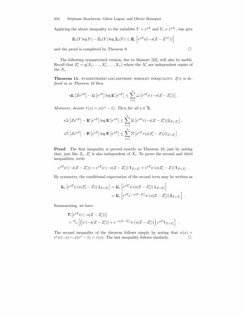
234 Stephane Boucheron, Gabor Lugosi, and Olivier Bousquet
Applying the above inequality to the variables Y = esZ and Yi = esZi , one gets
�i(Y log Y )− �
i(Y ) log�i(Y ) ≤ �
i
[esZψ(−s(Z − Z(i)))
]
and the proof is completed by Theorem 9. �
The following symmetrized version, due to Massart [23], will also be useful.Recall that Z ′
i = g(X1, . . . , X′i, . . . , Xn) where the X ′
i are independent copies ofthe Xi.
Theorem 11. symmetrized logarithmic sobolev inequality. If ψ is de-fined as in Theorem 10 then
s� [
ZesZ]− � [
esZ]
log� [
esZ]≤
n∑
i=1
� [esZψ (−s(Z − Z ′
i))].
Moreover, denote τ(x) = x(ex − 1). Then for all s ∈ �,
s� [
ZesZ]− � [
esZ]
log� [
esZ]≤
n∑
i=1
� [esZτ(−s(Z − Z ′
i))�
Z>Z′i
],
s� [
ZesZ]− � [
esZ]
log� [
esZ]≤
n∑
i=1
� [esZτ(s(Z ′
i − Z))�
Z<Z′i
].
Proof. The first inequality is proved exactly as Theorem 10, just by notingthat, just like Zi, Z
′i is also independent of Xi. To prove the second and third
inequalities, write
esZψ (−s(Z − Z ′i)) = esZψ (−s(Z − Z ′
i))�
Z>Z′i
+ esZψ (s(Z ′i − Z))
�
Z<Z′i.
By symmetry, the conditional expectation of the second term may be written as
�i
[esZψ (s(Z ′
i − Z))�
Z<Z′i
]=
�i
[esZ
′iψ (s(Z − Z ′
i))�
Z>Z′i
]
=�i
[esZe−s(Z−Z′
i)ψ (s(Z − Z ′i))
�
Z>Z′i
].
Summarizing, we have
� [esZψ (−s(Z − Z ′
i))]
=�i
[(ψ (−s(Z − Z ′
i)) + e−s(Z−Z′i)ψ (s(Z − Z ′
i)))esZ
�
Z>Z′i
].
The second inequality of the theorem follows simply by noting that ψ(x) +exψ(−x) = x(ex − 1) = τ(x). The last inequality follows similarly. �

Concentration Inequalities 235
3.4 First Example: Bounded Differences and More
The purpose of this section is to illustrate how the logarithmic Sobolev inequal-ities shown in the previous section may be used to obtain powerful exponentialconcentration inequalities. The first result is rather easy to obtain, yet it turnsout to be very useful. Also, its proof is prototypical, in the sense that it shows,in a transparent way, the main ideas.
Theorem 12. Assume that there exists a positive constant C such that, almostsurely,
n∑
i=1
(Z − Z ′i)
2 ≤ C .
Then for all t > 0,�
[|Z − �Z| > t] ≤ 2e−t
2/4C .
Proof. Observe that for x > 0, τ(−x) ≤ x2, and therefore, for any s > 0,Theorem 11 implies
s� [
ZesZ]− � [
esZ]
log� [
esZ]≤ �
[esZ
n∑
i=1
s2(Z − Z ′i)
2 �
Z>Z′i
]
≤ s2 �
[esZ
n∑
i=1
(Z − Z ′i)
2
]
≤ s2C � [esZ],
where at the last step we used the assumption of the theorem. Now denoting themoment generating function of Z by F (s) =
� [esZ], the above inequality may
be re-written assF ′(s)− F (s) logF (s) ≤ Cs2F (s) .
After dividing both sides by s2F (s), we observe that the left-hand side is justthe derivative of H(s) = s−1 logF (s), that is, we obtain the inequality
H ′(s) ≤ C .
By l’Hospital’s rule we note that lims→0H(s) = F ′(0)/F (0) =�Z, so by inte-
grating the above inequality, we get H(s) ≤ �Z + sC, or in other words,
F (s) ≤ es � Z+s2C .
Now by Markov’s inequality,
�[Z >
�Z + t] ≤ F (s)e−s � Z−st ≤ es2C−st .
Choosing s = t/2C, the upper bound becomes e−t2/4C . Replace Z by −Z to
obtain the same upper bound for�
[Z <�Z − t]. �

236 Stephane Boucheron, Gabor Lugosi, and Olivier Bousquet
Remark. It is easy to see that the condition of Theorem 12 may be relaxed inthe following way: if
�
[n∑
i=1
(Z − Z ′i)
2 �
Z>Z′i
∣∣∣X]≤ c
then for all t > 0,�
[Z >�Z + t] ≤ e−t2/4c
and if�
[n∑
i=1
(Z − Z ′i)
2 �
Z′i>Z
∣∣∣X]≤ c ,
then�
[Z <�Z − t] ≤ e−t2/4c .
An immediate corollary of Theorem 12 is a subgaussian tail inequality forfunctions of bounded differences.
Corollary 4. bounded differences inequality. Assume the function g sat-isfies the bounded differences assumption with constants c1, . . . , cn, then
�[|Z − �
Z| > t] ≤ 2e−t2/4C
where C =∑ni=1 c
2i .
We remark here that the constant appearing in this corollary may be im-proved. Indeed, using the martingale method, McDiarmid [2] showed that underthe conditions of Corollary 4,
�[|Z − �
Z| > t] ≤ 2e−2t2/C
(see the exercises). Thus, we have been able to extend Corollary 1 to an expo-nential concentration inequality. Note that by combining the variance bound ofCorollary 1 with Chebyshev’s inequality, we only obtained
�[|Z − �
Z| > t] ≤ C
2t2
and therefore the improvement is essential. Thus the applications of Corollary 1in all the examples shown in Section 2.1 are now improved in an essential waywithout further work.
However, Theorem 12 is much stronger than Corollary 4. To understand why,just observe that the conditions of Theorem 12 do not require that g has boundeddifferences. All that’s required is that
supx1,...,xn,x′1,...,x
′n∈X
n∑
i=1
|g(x1, . . . , xn)− g(x1, . . . , xi−1, x′i, xi+1, . . . , xn)|2 ≤
n∑
i=1
c2i ,
an obviously much milder requirement.

Concentration Inequalities 237
3.5 Exponential Inequalities for Self-bounding Functions
In this section we prove exponential concentration inequalities for self-boundingfunctions discussed in Section 2.2. Recall that a variant of the Efron-Stein in-equality (Theorem 2) implies that for self-bounding functions Var(Z) ≤ �
(Z) .Based on the logarithmic Sobolev inequality of Theorem 10 we may now obtainexponential concentration bounds. The theorem appears in Boucheron, Lugosi,and Massart [25] and builds on techniques developed by Massart [23].
Recall the definition of following two functions that we have already seen inBennett’s inequality and in the logarithmic Sobolev inequalities above:
h (u) = (1 + u) log (1 + u)− u (u ≥ −1),
and ψ(v) = supu≥−1
[uv − h(u)] = ev − v − 1 .
Theorem 13. Assume that g satisfies the self-bounding property. Then for everys ∈ �
,
log�[es(Z− � Z)
]≤ �
Zψ(s) .
Moreover, for every t > 0,
�[Z ≥ �
Z + t] ≤ exp
[− �
Zh
(t
�Z
)]
and for every 0 < t ≤ �Z,
�[Z ≤ �
Z − t] ≤ exp
[− �
Zh
(− t
�Z
)]
By recalling that h(u) ≥ u2/(2 + 2u/3) for u ≥ 0 (we have already used thisin the proof of Bernstein’s inequality) and observing that h(u) ≥ u2/2 for u ≤ 0,we obtain the following immediate corollaries: for every t > 0,
�[Z ≥ �
Z + t] ≤ exp
[− t2
2�Z + 2t/3
]
and for every 0 < t ≤ �Z,
�[Z ≤ �
Z − t] ≤ exp
[− t2
2�Z
].
Proof. We apply Lemma 10. Since the function ψ is convex with ψ (0) = 0, forany s and any u ∈ [0, 1] , ψ(−su) ≤ uψ(−s). Thus, since Z−Zi ∈ [0, 1], we havethat for every s, ψ(−s (Z − Zi)) ≤ (Z − Zi)ψ(−s) and therefore, Lemma 10 andthe condition
∑ni=1(Z − Zi) ≤ Z imply that
s� [
ZesZ]− � [
esZ]
log� [
esZ]≤ �
[ψ(−s)esZ
n∑
i=1
(Z − Zi)]
≤ ψ(−s) � [ZesZ
].
238 Stephane Boucheron, Gabor Lugosi, and Olivier Bousquet
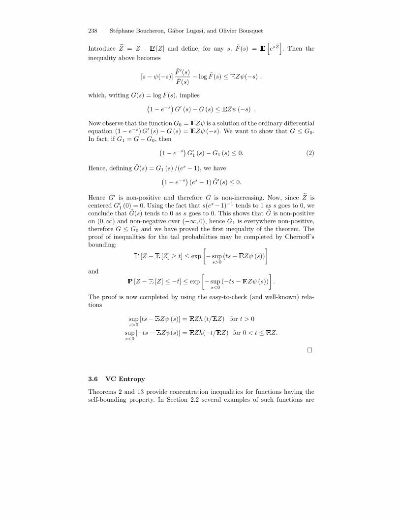
Introduce Z = Z − �[Z] and define, for any s, F (s) =
�[es
eZ]. Then the
inequality above becomes
[s− ψ(−s)] F′(s)
F (s)− log F (s) ≤ �
Zψ(−s) ,
which, writing G(s) = logF (s), implies
(1− e−s
)G′ (s)−G (s) ≤ �
Zψ (−s) .
Now observe that the functionG0 =�Zψ is a solution of the ordinary differential
equation (1− e−s)G′ (s) − G (s) =�Zψ (−s). We want to show that G ≤ G0.
In fact, if G1 = G−G0, then
(1− e−s
)G′
1 (s)−G1 (s) ≤ 0. (2)
Hence, defining G(s) = G1 (s) /(es − 1), we have
(1− e−s
)(es − 1) G′(s) ≤ 0.
Hence G′ is non-positive and therefore G is non-increasing. Now, since Z iscentered G′
1 (0) = 0. Using the fact that s(es−1)−1 tends to 1 as s goes to 0, weconclude that G(s) tends to 0 as s goes to 0. This shows that G is non-positiveon (0,∞) and non-negative over (−∞, 0), hence G1 is everywhere non-positive,therefore G ≤ G0 and we have proved the first inequality of the theorem. Theproof of inequalities for the tail probabilities may be completed by Chernoff’sbounding:
�[Z − �
[Z] ≥ t] ≤ exp
[− sups>0
(ts− �Zψ (s))
]
and�
[Z − �[Z] ≤ −t] ≤ exp
[− sups<0
(−ts− �Zψ (s))
].
The proof is now completed by using the easy-to-check (and well-known) rela-tions
sups>0
[ts− �Zψ (s)] =
�Zh (t/
�Z) for t > 0
sups<0
[−ts− �Zψ(s)] =
�Zh(−t/ �
Z) for 0 < t ≤ �Z.
�
3.6 VC Entropy
Theorems 2 and 13 provide concentration inequalities for functions having theself-bounding property. In Section 2.2 several examples of such functions are
Concentration Inequalities 239
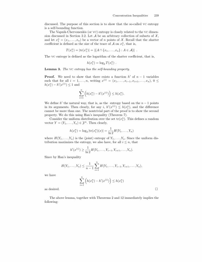
discussed. The purpose of this section is to show that the so-called vc entropyis a self-bounding function.
The Vapnik-Chervonenkis (or vc) entropy is closely related to the vc dimen-sion discussed in Section 2.2. Let A be an arbitrary collection of subsets of X ,and let xn1 = (x1, . . . , xn) be a vector of n points of X . Recall that the shatter
coefficient is defined as the size of the trace of A on xn1 , that is,
T (xn1 ) = |tr(xn1 )| = |{A ∩ {x1, . . . , xn} : A ∈ A}| .The vc entropy is defined as the logarithm of the shatter coefficient, that is,
h(xn1 ) = log2 T (xn1 ) .
Lemma 3. The vc entropy has the self-bounding property.
Proof. We need to show that there exists a function h′ of n − 1 variablessuch that for all i = 1, . . . , n, writing x(i) = (x1, . . . , xi−1, xi+1, . . . , xn), 0 ≤h(xn1 )− h′(x(i)) ≤ 1 and
n∑
i=1
(h(xn1 )− h′(x(i))
)≤ h(xn1 ).
We define h′ the natural way, that is, as the entropy based on the n− 1 pointsin its arguments. Then clearly, for any i, h′(x(i)) ≤ h(xn1 ), and the differencecannot be more than one. The nontrivial part of the proof is to show the secondproperty. We do this using Han’s inequality (Theorem 7).
Consider the uniform distribution over the set tr(xn1 ). This defines a randomvector Y = (Y1, . . . , Yn) ∈ Yn. Then clearly,
h(xn1 ) = log2 |tr(xn1 )(x)| = 1
ln 2H(Y1, . . . , Yn)
where H(Y1, . . . , Yn) is the (joint) entropy of Y1, . . . , Yn. Since the uniform dis-tribution maximizes the entropy, we also have, for all i ≤ n, that
h′(x(i)) ≥ 1
ln 2H(Y1, . . . , Yi−1, Yi+1, . . . , Yn).
Since by Han’s inequality
H(Y1, . . . , Yn) ≤ 1
n− 1
n∑
i=1
H(Y1, . . . , Yi−1, Yi+1, . . . , Yn),
we haven∑
i=1
(h(xn1 )− h′(x(i))
)≤ h(xn1 )
as desired. �
The above lemma, together with Theorems 2 and 12 immediately implies thefollowing:

240 Stephane Boucheron, Gabor Lugosi, and Olivier Bousquet
Corollary 5. Let X1, . . . , Xn be independent random variables taking their val-ues in X and let Z = h(Xn
1 ) denote the random vc entropy. Then Var(Z) ≤�
[Z], for t > 0
�[Z ≥ �
Z + t] ≤ exp
[− t2
2�Z + 2t/3
],
and for every 0 < t ≤ �Z,
�[Z ≤ �
Z − t] ≤ exp
[− t2
2�Z
].
Moreover, for the random shatter coefficient T (Xn1 ), we have
�log2 T (Xn
1 ) ≤ log2
�T (Xn
1 ) ≤ log2 e�
log2 T (Xn1 ) .
Note that the left-hand side of the last statement follows from Jensen’s in-equality, while the right-hand side by taking s = ln 2 in the first inequality of The-orem 13. This last statement shows that the expected vc entropy
�log2 T (Xn
1 )and the annealed vc entropy are tightly connected, regardless of the class of setsA and the distribution of the Xi’s. We note here that this fact answers, in apositive way, an open question raised by Vapnik [69, pages 53–54]: the empiricalrisk minimization procedure is non-trivially consistent and rapidly convergent ifand only if the annealed entropy rate (1/n) log2
�[T (X)] converges to zero. For
the definitions and discussion we refer to [69].
3.7 Variations on the Theme
In this section we show how the techniques of the entropy method for provingconcentration inequalities may be used in various situations not considered sofar. The versions differ in the assumptions on how
∑ni=1(Z − Z ′
i)2 is controlled
by different functions of Z. For various other versions with applications we referto Boucheron, Lugosi, and Massart [26]. In all cases the upper bound is roughly
of the form e−t2/σ2
where σ2 is the corresponding Efron-Stein upper bound onVar(Z). The first inequality may be regarded as a generalization of the uppertail inequality in Theorem 13.
Theorem 14. Assume that there exist positive constants a and b such that
n∑
i=1
(Z − Z ′i)
2 �
Z>Z′i≤ aZ + b .
Then for s ∈ (0, 1/a),
log�
[exp(s(Z − �[Z]))] ≤ s2
1− as (a�Z + b)
and for all t > 0,
� {Z >�Z + t} ≤ exp
( −t24a
�Z + 4b+ 2at
).

Concentration Inequalities 241
Proof. Let s > 0. Just like in the first steps of the proof of Theorem 12, we usethe fact that for x > 0, τ(−x) ≤ x2, and therefore, by Theorem 11 we have
s� [
ZesZ]− � [
esZ]
log� [
esZ]≤ �
[esZ
n∑
i=1
(Z − Z ′i)
2 �
Z>Z′i
]
≤ s2(a
� [ZesZ
]+ b
� [esZ])
,
where at the last step we used the assumption of theorem.Denoting, once again, F (s) =
� [esZ], the above inequality becomes
sF ′(s)− F (s) logF (s) ≤ as2F ′(s) + bs2F (s) .
After dividing both sides by s2F (s), once again we see that the left-hand side isjust the derivative of H(s) = s−1 logF (s), so we obtain
H ′(s) ≤ a(logF (s))′ + b .
Using the fact that lims→0H(s) = F ′(0)/F (0) =�Z and logF (0) = 0, and
integrating the inequality, we obtain
H(s) ≤ �Z + a logF (s) + bs ,
or, if s < 1/a,
log�
[s(Z − �[Z])] ≤ s2
1− as (a�Z + b) ,
proving the first inequality. The inequality for the upper tail now follows byMarkov’s inequality and the following technical lemma whose proof is left as anexercise. �
Lemma 4. Let C and a denote two positive real numbers and denote h1(x) =1 + x−
√1 + 2x. Then
supλ∈[0,1/a)
(λt− Cλ2
1− aλ
)=
2C
a2h1
(at
2C
)≥ t2
2(2C + at
)
and the supremum is attained at
λ =1
a
(1−
(1 +
at
C
)−1/2)
.
Also,
supλ∈[0,∞)
(λt− Cλ2
1 + aλ
)=
2C
a2h1
(−at2C
)≥ t2
4C
if t < C/a and the supremum is attained at
λ =1
a
((1− at
C
)−1/2
− 1
).

242 Stephane Boucheron, Gabor Lugosi, and Olivier Bousquet
There is a subtle difference between upper and lower tail bounds. Boundsfor the lower tail
� {Z <�Z − t} may be easily derived, due to Chebyshev’s
association inequality which states that if X is a real-valued random variableand f is a nonincreasing and g is a nondecreasing function, then
�[f(X)g(X)] ≤ �
[f(X)]�
[g(X)]| .
Theorem 15. Assume that for some nondecreasing function g,
n∑
i=1
(Z − Z ′i)
2 �
Z<Z′i≤ g(Z) .
Then for all t > 0,
�[Z <
�Z − t] ≤ exp
( −t24
�[g(Z)]
).
Proof. To prove lower-tail inequalities we obtain upper bounds for F (s) =�
[exp(sZ)] with s < 0. By the third inequality of Theorem 11,
s� [
ZesZ]− � [
esZ]
log� [
esZ]
≤n∑
i=1
� [esZτ(s(Z ′
i − Z))�
Z<Z′i
]
≤n∑
i=1
� [esZs2(Z ′
i − Z)2�
Z<Z′i
]
(using s < 0 and that τ(−x) ≤ x2 for x > 0)
= s2�
[esZ
n∑
i=1
(Z − Z ′i)
2 �
Z<Z′i
]
≤ s2 � [esZg(Z)
].
Since g(Z) is a nondecreasing and esZ is a decreasing function of Z, Chebyshev’sassociation inequality implies that
� [esZg(Z)
]≤ � [
esZ] �
[g(Z)] .
Thus, dividing both sides of the obtained inequality by s2F (s) and writingH(s) = (1/s) logF (s), we obtain
H ′(s) ≤ �[g(Z)] .
Integrating the inequality in the interval [s, 0) we obtain
F (s) ≤ exp(s2�
[g(Z)] + s�
[Z]) .
Markov’s inequality and optimizing in s now implies the theorem. �

Concentration Inequalities 243
The next result is useful when one is interested in lower-tail bounds but∑ni=1(Z − Z ′
i)2 �
Z<Z′i
is difficult to handle. In some cases∑ni=1(Z − Z ′
i)2 �
Z>Z′i
is easier to bound. In such a situation we need the additional guarantee that|Z−Z ′
i| remains bounded. Without loss of generality, we assume that the boundis 1.
Theorem 16. Assume that there exists a nondecreasing function g such that∑ni=1(Z − Z ′
i)2 �
Z>Z′i≤ g(Z) and for any value of Xn
1 and Xi′, |Z − Z ′
i| ≤ 1.Then for all K > 0, s ∈ [0, 1/K)
log� [
exp(−s(Z − �[Z]))
]≤ s2 τ(K)
K2
�[g(Z)] ,
and for all t > 0, with t ≤ (e− 1)�
[g(Z)] we have
�[Z <
�Z − t] ≤ exp
(− t2
4(e− 1)�
[g(Z)]
).
Proof. The key observation is that the function τ(x)/x2 = (ex − 1)/x is in-creasing if x > 0. Choose K > 0. Thus, for s ∈ (−1/K, 0), the second inequalityof Theorem 11 implies that
s� [
ZesZ]− � [
esZ]
log� [
esZ]≤
n∑
i=1
�[esZτ(−s(Z − Z(i)))
�
Z>Z′i
]
≤ s2 τ(K)
K2
�
[esZ
n∑
i=1
(Z − Z(i))2�
Z>Z′i
]
≤ s2 τ(K)
K2
� [g(Z)esZ
],
where at the last step we used the assumption of the theorem.Just like in the proof of Theorem 15, we bound
� [g(Z)esZ
]by
�[g(Z)]
� [esZ].
The rest of the proof is identical to that of Theorem 15. Here we took K = 1. �
Finally we give, without proof, an inequality (due to Bousquet [28]) forfunctions satisfying conditions similar but weaker than the self-bounding con-ditions. This is very useful for suprema of empirical processes for which thenon-negativity assumption does not hold.
Theorem 17. Assume Z satisfies∑ni=1 Z − Zi ≤ Z, and there exist random
variables Yi such that for all i = 1, . . . , n, Yi ≤ Z − Zi ≤ 1, Yi ≤ a for somea > 0 and
�iYi ≥ 0. Also, let σ2 be a real number such that
σ2 ≥ 1
n
n∑
i=1
�i[Y
2i ] .

244 Stephane Boucheron, Gabor Lugosi, and Olivier Bousquet
We obtain for all t > 0,
� {Z ≥ �Z + t} ≤ exp
(−vh
(t
v
)),
where v = (1 + a)�Z + nσ2.
An important application of the above theorem is the following version of Tala-grand’s concentration inequality for empirical processes. The constants appear-ing here were obtained by Bousquet [27].
Corollary 6. Let F be a set of functions that satisfy�f(Xi) = 0 and supf∈F
sup f ≤ 1. We denote
Z = supf∈F
n∑
i=1
f(Xi) .
Let σ be a positive real number such that nσ2 ≥ ∑ni=1 supf∈F
�[f2(Xi)], then
for all t ≥ 0, we have
� {Z ≥ �Z + t} ≤ exp
(−vh
(t
v
)),
with v = nσ2 + 2�Z.
References
1. Milman, V., Schechman, G.: Asymptotic theory of finite-dimensional normedspaces. Springer-Verlag, New York (1986)
2. McDiarmid, C.: On the method of bounded differences. In: Surveys in Combina-torics 1989, Cambridge University Press, Cambridge (1989) 148–188
3. McDiarmid, C.: Concentration. In Habib, M., McDiarmid, C., Ramirez-Alfonsin,J., Reed, B., eds.: Probabilistic Methods for Algorithmic Discrete Mathematics,Springer, New York (1998) 195–248
4. Ahlswede, R., Gacs, P., Korner, J.: Bounds on conditional probabilities with ap-plications in multi-user communication. Zeitschrift fur Wahrscheinlichkeitstheorieund verwandte Gebiete 34 (1976) 157–177 (correction in 39:353–354,1977).
5. Marton, K.: A simple proof of the blowing-up lemma. IEEE Transactions onInformation Theory 32 (1986) 445–446
6. Marton, K.: Bounding d-distance by informational divergence: a way to provemeasure concentration. Annals of Probability 24 (1996) 857–866
7. Marton, K.: A measure concentration inequality for contracting Markov chains.Geometric and Functional Analysis 6 (1996) 556–571 Erratum: 7:609–613, 1997.
8. Dembo, A.: Information inequalities and concentration of measure. Annals ofProbability 25 (1997) 927–939
9. Massart, P.: Optimal constants for Hoeffding type inequalities. Technical report,Mathematiques, Universite de Paris-Sud, Report 98.86 (1998)
10. Rio, E.: Inegalites de concentration pour les processus empiriques de classes departies. Probability Theory and Related Fields 119 (2001) 163–175

Concentration Inequalities 245
11. Talagrand, M.: Concentration of measure and isoperimetric inequalities in productspaces. Publications Mathematiques de l’I.H.E.S. 81 (1995) 73–205
12. Talagrand, M.: New concentration inequalities in product spaces. InventionesMathematicae 126 (1996) 505–563
13. Talagrand, M.: A new look at independence. Annals of Probability 24 (1996) 1–34(Special Invited Paper).
14. Luczak, M.J., McDiarmid, C.: Concentration for locally acting permutations. Dis-crete Mathematics (2003) to appear
15. McDiarmid, C.: Concentration for independent permutations. Combinatorics,Probability, and Computing 2 (2002) 163–178
16. Panchenko, D.: A note on Talagrand’s concentration inequality. Electronic Com-munications in Probability 6 (2001)
17. Panchenko, D.: Some extensions of an inequality of Vapnik and Chervonenkis.Electronic Communications in Probability 7 (2002)
18. Panchenko, D.: Symmetrization approach to concentration inequalities for empir-ical processes. Annals of Probability to appear (2003)
19. de la Pena, V., Gine, E.: Decoupling: from Dependence to Independence. Springer,New York (1999)
20. Ledoux, M.: On Talagrand’s deviation inequalities for product measures. ESAIM:Probability and Statistics 1 (1997) 63–87 http://www.emath.fr/ps/.
21. Ledoux, M.: Isoperimetry and Gaussian analysis. In Bernard, P., ed.: Lectures onProbability Theory and Statistics, Ecole d’Ete de Probabilites de St-Flour XXIV-1994 (1996) 165–294
22. Bobkov, S., Ledoux, M.: Poincare’s inequalities and Talagrands’s concentrationphenomenon for the exponential distribution. Probability Theory and RelatedFields 107 (1997) 383–400
23. Massart, P.: About the constants in Talagrand’s concentration inequalities forempirical processes. Annals of Probability 28 (2000) 863–884
24. Klein, T.: Une inegalite de concentration a gauche pour les processus empiriques.C. R. Math. Acad. Sci. Paris 334 (2002) 501–504
25. Boucheron, S., Lugosi, G., Massart, P.: A sharp concentration inequality withapplications. Random Structures and Algorithms 16 (2000) 277–292
26. Boucheron, S., Lugosi, G., Massart, P.: Concentration inequalities using the en-tropy method. The Annals of Probability 31 (2003) 1583–1614
27. Bousquet, O.: A Bennett concentration inequality and its application to supremaof empirical processes. C. R. Acad. Sci. Paris 334 (2002) 495–500
28. Bousquet, O.: Concentration inequalities for sub-additive functions using the en-tropy method. In Gine, E., C.H., Nualart, D., eds.: Stochastic Inequalities andApplications. Volume 56 of Progress in Probability. Birkhauser (2003) 213–247
29. Boucheron, S., Bousquet, O., Lugosi, G., Massart, P.: Moment inequalities forfunctions of independent random variables. The Annals of Probability (2004) toappear.
30. Janson, S., Luczak, T., Rucinski, A.: Random graphs. John Wiley, New York(2000)
31. Hoeffding, W.: Probability inequalities for sums of bounded random variables.Journal of the American Statistical Association 58 (1963) 13–30
32. Chernoff, H.: A measure of asymptotic efficiency of tests of a hypothesis based onthe sum of observations. Annals of Mathematical Statistics 23 (1952) 493–507
33. Okamoto, M.: Some inequalities relating to the partial sum of binomial probabili-ties. Annals of the Institute of Statistical Mathematics 10 (1958) 29–35

246 Stephane Boucheron, Gabor Lugosi, and Olivier Bousquet
34. Bennett, G.: Probability inequalities for the sum of independent random variables.Journal of the American Statistical Association 57 (1962) 33–45
35. Bernstein, S.: The Theory of Probabilities. Gastehizdat Publishing House, Moscow(1946)
36. Efron, B., Stein, C.: The jackknife estimate of variance. Annals of Statistics 9(1981) 586–596
37. Steele, J.: An Efron-Stein inequality for nonsymmetric statistics. Annals of Statis-tics 14 (1986) 753–758
38. Vapnik, V., Chervonenkis, A.: On the uniform convergence of relative frequenciesof events to their probabilities. Theory of Probability and its Applications 16(1971) 264–280
39. Devroye, L., Gyorfi, L., Lugosi, G.: A Probabilistic Theory of Pattern Recognition.Springer-Verlag, New York (1996)
40. Vapnik, V.: Statistical Learning Theory. John Wiley, New York (1998)41. van der Waart, A., Wellner, J.: Weak convergence and empirical processes.
Springer-Verlag, New York (1996)42. Dudley, R.: Uniform Central Limit Theorems. Cambridge University Press, Cam-
bridge (1999)43. Koltchinskii, V., Panchenko, D.: Empirical margin distributions and bounding the
generalization error of combined classifiers. Annals of Statistics 30 (2002)44. Massart, P.: Some applications of concentration inequalities to statistics. Annales
de la Faculte des Sciencies de Toulouse IX (2000) 245–30345. Bartlett, P., Boucheron, S., Lugosi, G.: Model selection and error estimation.
Machine Learning 48 (2001) 85–11346. Lugosi, G., Wegkamp, M.: Complexity regularization via localized random penal-
ties. submitted (2003)47. Bousquet, O.: New approaches to statistical learning theory. Annals of the Institute
of Statistical Mathematics 55 (2003) 371–38948. Lugosi, G.: Pattern classification and learning theory. In Gyorfi, L., ed.: Principles
of Nonparametric Learning, Springer, Viena (2002) 5–6249. Devroye, L., Gyorfi, L.: Nonparametric Density Estimation: The L1 View. John
Wiley, New York (1985)50. Devroye, L.: The kernel estimate is relatively stable. Probability Theory and
Related Fields 77 (1988) 521–53651. Devroye, L.: Exponential inequalities in nonparametric estimation. In Roussas, G.,
ed.: Nonparametric Functional Estimation and Related Topics, NATO ASI Series,Kluwer Academic Publishers, Dordrecht (1991) 31–44
52. Devroye, L., Lugosi, G.: Combinatorial Methods in Density Estimation. Springer-Verlag, New York (2000)
53. Koltchinskii, V.: Rademacher penalties and structural risk minimization. IEEETransactions on Information Theory 47 (2001) 1902–1914
54. Bartlett, P., Mendelson, S.: Rademacher and Gaussian complexities: risk boundsand structural results. Journal of Machine Learning Research 3 (2002) 463–482
55. Bartlett, P., Bousquet, O., Mendelson, S.: Localized Rademacher complexities.In: Proceedings of the 15th annual conference on Computational Learning Theory.(2002) 44–48
56. Vapnik, V., Chervonenkis, A.: Theory of Pattern Recognition. Nauka, Moscow(1974) (in Russian); German translation: Theorie der Zeichenerkennung, AkademieVerlag, Berlin, 1979.
57. Blumer, A., Ehrenfeucht, A., Haussler, D., Warmuth, M.: Learnability and theVapnik-Chervonenkis dimension. Journal of the ACM 36 (1989) 929–965

Concentration Inequalities 247
58. Anthony, M., Bartlett, P.L.: Neural Network Learning: Theoretical Foundations.Cambridge University Press, Cambridge (1999)
59. Rhee, W., Talagrand, M.: Martingales, inequalities, and NP-complete problems.Mathematics of Operations Research 12 (1987) 177–181
60. Shamir, E., Spencer, J.: Sharp concentration of the chromatic number on randomgraphs gn,p. Combinatorica 7 (1987) 374–384
61. Samson, P.M.: Concentration of measure inequalities for Markov chains and φ-mixing processes. Annals of Probability 28 (2000) 416–461
62. Cover, T., Thomas, J.: Elements of Information Theory. John Wiley, New York(1991)
63. Han, T.: Nonnegative entropy measures of multivariate symmetric correlations.Information and Control 36 (1978)
64. Beckner, W.: A generalized Poincare inequality for Gaussian measures. Proceed-ings of the American Mathematical Society 105 (1989) 397–400
65. Lata la, R., Oleszkiewicz, C.: Between Sobolev and Poincare. In: Geometric Aspectsof Functional Analysis, Israel Seminar (GAFA), 1996-2000, Springer (2000) 147–168 Lecture Notes in Mathematics, 1745.
66. Chafaı, D.: On φ-entropies and φ-Sobolev inequalities. Technical report,arXiv.math.PR/0211103 (2002)
67. Ledoux, M.: Concentration of measure and logarithmic sobolev inequalities. In:Seminaire de Probabilites XXXIII. Lecture Notes in Mathematics 1709, Springer(1999) 120–216
68. Ledoux, M.: The concentration of measure phenomenon. American MathematicalSociety, Providence, RI (2001)
69. Vapnik, V.: The Nature of Statistical Learning Theory. Springer-Verlag, New York(1995)