SYMMETRIC INDEFINITE MATRICES:LINEAR SYSTEM SOLVERSANDMODIFIED INERTIA PROBLEMSA thesis submitted to the University of Manchesterfor the degree of Doctor of Philosophyin the Faculty of Science and Engineering

January 1998BySheung Hun ChengDepartment of Mathematics

ContentsCopyright 7Abstract 8Declaration 10Acknowledgements 111 Introduction 121.1 Symmetric Inde�nite Matrices and Numerical Analysis . . . . . . 121.2 Floating Point Arithmetic . . . . . . . . . . . . . . . . . . . . . . 131.3 Model of Arithmetic . . . . . . . . . . . . . . . . . . . . . . . . . 141.4 IEEE Arithmetic . . . . . . . . . . . . . . . . . . . . . . . . . . . 151.5 Perturbation Theory . . . . . . . . . . . . . . . . . . . . . . . . . 171.6 Overview . . . . . . . . . . . . . . . . . . . . . . . . . . . . . . . . 202 Accuracy and Stability of the Diagonal Pivoting Method 232.1 Introduction . . . . . . . . . . . . . . . . . . . . . . . . . . . . . . 232.2 Pivoting Strategies . . . . . . . . . . . . . . . . . . . . . . . . . . 242.3 The Growth Factor . . . . . . . . . . . . . . . . . . . . . . . . . . 292.4 Error Analysis . . . . . . . . . . . . . . . . . . . . . . . . . . . . . 322.4.1 Normwise Backward Stability . . . . . . . . . . . . . . . . 322.4.2 Componentwise Backward Stability . . . . . . . . . . . . . 332.4.3 BK Beats BBK . . . . . . . . . . . . . . . . . . . . . . . . 342.4.4 BBK Beats BK . . . . . . . . . . . . . . . . . . . . . . . . 352.4.5 Normwise and Componentwise Forward Stability . . . . . 362.5 The Role of Ashcraft, Grimes and Lewis Example . . . . . . . . . 392

Contents2.6 Concluding Remarks . . . . . . . . . . . . . . . . . . . . . . . . . 433 Accuracy and Stability of Aasen's Method 453.1 Introduction . . . . . . . . . . . . . . . . . . . . . . . . . . . . . . 453.2 The Parlett and Reid Method . . . . . . . . . . . . . . . . . . . . 473.3 Aasen's Method . . . . . . . . . . . . . . . . . . . . . . . . . . . . 483.4 Numerical Stability . . . . . . . . . . . . . . . . . . . . . . . . . . 503.5 The Growth Factor . . . . . . . . . . . . . . . . . . . . . . . . . . 513.6 Concluding Remarks . . . . . . . . . . . . . . . . . . . . . . . . . 534 Modi�ed Cholesky Algorithms 544.1 Introduction . . . . . . . . . . . . . . . . . . . . . . . . . . . . . . 544.2 The Gill, Murray and Wright Algorithm . . . . . . . . . . . . . . 574.3 The Schnabel and Eskow Algorithm . . . . . . . . . . . . . . . . . 604.4 The New Modi�ed Cholesky Algorithm . . . . . . . . . . . . . . . 654.5 The Modi�ed Aasen Algorithm . . . . . . . . . . . . . . . . . . . 714.5.1 Solving Symmetric Tridiagonal Eigenproblem . . . . . . . 724.6 Comparison of Algorithms . . . . . . . . . . . . . . . . . . . . . . 764.7 Numerical Experiments . . . . . . . . . . . . . . . . . . . . . . . . 774.8 Concluding Remarks . . . . . . . . . . . . . . . . . . . . . . . . . 855 Modifying the Inertia of Matrices Arising in Optimization 875.1 Introduction . . . . . . . . . . . . . . . . . . . . . . . . . . . . . . 875.2 A Symmetric Block 2� 2 Matrix and its Applications . . . . . . . 885.3 Rectangular Congruence Transformations . . . . . . . . . . . . . . 925.4 Inertia Properties of C . . . . . . . . . . . . . . . . . . . . . . . . 955.5 Modifying the Inertia: A General Perturbation . . . . . . . . . . . 985.6 Modifying the Inertia: A Structured Perturbation . . . . . . . . . 995.7 A Projected Hessian Approach . . . . . . . . . . . . . . . . . . . . 1043

Contents5.8 Practical Algorithm . . . . . . . . . . . . . . . . . . . . . . . . . . 1075.9 Numerical Experiments . . . . . . . . . . . . . . . . . . . . . . . . 1095.10 Concluding Remarks . . . . . . . . . . . . . . . . . . . . . . . . . 1116 Generalized Hermitian Eigenvalue Problems 1136.1 Introduction . . . . . . . . . . . . . . . . . . . . . . . . . . . . . . 1136.2 Properties of Hermitian Matrix Product . . . . . . . . . . . . . . 1146.3 De�nite Pairs . . . . . . . . . . . . . . . . . . . . . . . . . . . . . 1196.4 Simultaneous Diagonalization . . . . . . . . . . . . . . . . . . . . 1236.4.1 When A and B are Banded . . . . . . . . . . . . . . . . . 1246.5 Nearest De�nite Pair . . . . . . . . . . . . . . . . . . . . . . . . . 1286.5.1 Optimal 2-norm Perturbations . . . . . . . . . . . . . . . . 1296.5.2 Normal Pairs . . . . . . . . . . . . . . . . . . . . . . . . . 1366.6 Concluding Remarks . . . . . . . . . . . . . . . . . . . . . . . . . 139Bibliography 141

4

List of Tables1.1 Floating point formats for single and double precision in IEEEarithmetic. . . . . . . . . . . . . . . . . . . . . . . . . . . . . . . . 151.2 IEEE arithmetic exceptions and default results. . . . . . . . . . . 162.1 Backward error for computed solution of symmetric inde�nite sys-tems of dimension 3. . . . . . . . . . . . . . . . . . . . . . . . . . 362.2 Parameterization of scaled test matrices. . . . . . . . . . . . . . . 404.1 The eigenvalues of matrix (4.19) and the block diagonal matrix eDwhen the BBK and BK pivoting strategies are used. . . . . . . . . 684.2 Method of choice for symmetric tridiagonal matrix T . . . . . . . . 754.3 Measures of E for the 4� 4 matrix (4.29). . . . . . . . . . . . . . 794.4 Number of comparisons for the BBK pivoting strategy. . . . . . . 796.1 Properties of matrix product M = B�1A. . . . . . . . . . . . . . . 119

5

List of Figures1.1 Backward and forward stability. . . . . . . . . . . . . . . . . . . . 192.1 Matrices for which the entire remaining submatrix must be searchedat each step of the BBK strategy. . . . . . . . . . . . . . . . . . . 292.2 Scaling parameter for each entry of test matrix. . . . . . . . . . . 402.3 Comparison of relative normwise forward error on scaled N(0; 1)matrices with m = 3, n = 50. . . . . . . . . . . . . . . . . . . . . 412.4 Comparison of relative componentwise forward error bound onscaled N(0; 1) matrices with m = 3, n = 50. . . . . . . . . . . . . 422.5 Comparison of relative componentwise forward error bound onscaled N(0; 1) matrices with m = 3, n = 50. . . . . . . . . . . . . 424.1 Measures of E for 30 random inde�nite matrices with n = 25. . . 804.2 Measures of E for 30 random inde�nite matrices with n = 50. . . 804.3 Measures of E for 30 random inde�nite matrices with n = 100. . . 814.4 Condition numbers �2(A + E) for 30 random inde�nite matriceswith n = 25. . . . . . . . . . . . . . . . . . . . . . . . . . . . . . . 814.5 Condition numbers �2(A + E) for 30 random inde�nite matriceswith n = 50. . . . . . . . . . . . . . . . . . . . . . . . . . . . . . . 824.6 Condition numbers �2(A + E) for 30 random inde�nite matriceswith n = 100. . . . . . . . . . . . . . . . . . . . . . . . . . . . . . 824.7 Measures for three nonrandom matrices. . . . . . . . . . . . . . . 836.1 Change of boundaries of the �eld of values under perturbation(6.16), (6.17). . . . . . . . . . . . . . . . . . . . . . . . . . . . . . 1356.2 A typical graph �max(A�) for an inde�nite pair (A;B). . . . . . . 1366.3 The �eld of values of normal pair (6:19) . . . . . . . . . . . . . . . 1396

CopyrightCopyright in text of this thesis rests with the Author. Copies (by any process)either in full, or of extracts, may be made only in accordance with instruc-tions given by the Author and lodged in the John Rylands University Library ofManchester. Details may be obtained from the Librarian. This page must formpart of any such copies made. Further copies (by any process) of copies made inaccordance with such instructions may not be made without the permission (inwriting) of the Author.The ownership of any intellectual property rights which may be describedin this thesis is vested in the University of Manchester, subject to any prioragreement to the contrary, and may not be made available for use by third partieswithout the written permission of the University, which will prescribe the termsand conditions of any such agreement.Further information on the conditions under which disclosures and exploita-tion may take place is available from the head of Department of Mathematics.

7

AbstractSymmetric inde�nite matrices are an important class of matrices arising in manyapplications. Some practically important computations associated with this classof matrices are investigated in this thesis.First our emphasis is on examining the accuracy and stability of the twomost popular methods for solving symmetric inde�nite linear systems, namelythe diagonal pivoting method and Aasen's method. Suitable pivoting strategiesare crucial to the stability of both methods. For the diagonal pivoting method,we assess the Bunch{Kaufman and the more recent bounded Bunch{Kaufmanpivoting strategies using various stability measures. We con�rm that the boundedBunch{Kaufman pivoting strategy achieves better accuracy for a set of examples.However, theoretical analyses and experimental results show that the \superior"accuracy that has been claimed is not fully justi�ed.For Aasen's method, a new normwise backward stability result of Highamis stated. We derive a growth factor bound which is attainable for matrices ofdimension 3. Direct search methods are employed to search for large growthfactors to gain insight into the behaviour of the growth factor of Aasen's method.Our focus is then on tackling three modi�ed inertia problems. We propose twoalternative modi�ed Cholesky algorithms based on the two previously mentionedlinear solvers, and compare their performance with the two existing algorithmsof Gill, Murray and Wright, and Schnabel and Eskow, both theoretically and nu-merically. The experimental results show that all four algorithms are competitive.Our algorithms have the advantages of ease of implementation and the existenceof a priori bounds for assessing how \good" the perturbation is.Motivated by an application in constrained optimization, we then concentrateon deriving structured perturbations for a block 2� 2 matrix A, which involves8

List of Figuresperturbing the (1; 1) block so that A has a particular inertia. We derive a per-turbation, valid for any unitarily invariant norm, that increases the number ofnonnegative eigenvalues by a given amount. An alternative approach based ona projection into the null space of the constraints is also considered. Theoreti-cal tools developed include an extension of Ostrowski's theorem on congruencetransformations and some lemmas on inertia properties of block 2� 2 matrices.Finally the generalized Hermitian eigenvalue problem is discussed. We clearsome confusion on the characteristics of the eigenvalues of Hermitian matrix prod-ucts. A new concept called the inner numerical radius is introduced, using whichwe derive an elegant solution to the nearness problem of �nding the distance froman inde�nite matrix pair to the nearest de�nite pair in the 2-norm. An alterna-tive approach for determining the inner numerical radius of a normal pair, whichexploits the characteristics of its eigenvalues, is proposed.

9

DeclarationNo portion of the work referred to in this thesis has been submitted in support ofan application for another degree or quali�cation of this or any other universityor other institution of learning.� Chapter 4 is based on the technical report \A modi�ed Cholesky algorithmbased on a symmetric inde�nite factorization" (with Nicholas J. Higham)[17], 1996. This work is to appear in SIAM J. Matrix Anal. Appl..� Chapter 5 is based on the technical report \Modifying the inertia of matricesarising in optimization" (with Nicholas J. Higham) [59], 1996. This work isto appear in Linear Algebra and Appl..� Section 6.5 is based on the technical report in preparation \De�nite pairsand the inner numerical radius" (with Nicholas J. Higham) [18], 1997.

10

AcknowledgementsIn writing this thesis I have been helped and in uenced by many people. Iam particularly indebted to Nick Higham for his unfailing patience, constantinspiration and fruitful perturbation on my thesis. I thank him.Special thanks to Phil Jacob for making my stay in Manchester such an enjoy-able experience, and Tony Cox for numerous lively and intriguing conversations.Thanks also goes to my Mum and Dad, Betty, Amy and Carmen for theirunconditional love and support.Amongst these wonderful people whose presence made this thesis possible,it is a pleasure to thank Gigi Chao, Frances and Shun Cheung, Clare Chiu,Phil Davies, Michaela Gruber, Wendy Hall, Kathrin Happe, Angela Henderson,Setsuko Matsumoto, Lorraine Seymour, Kath Smith, Elena Takeuchi, the Pete'sEat, the Cornerhouse cinema and the Greenhouse restaurant.I acknowledge the Committee of Vice-Chancellors and Principals of the Uni-versities of the United Kingdom for the support of an Overseas Research StudentAward, and Hulme Hall for a Postgraduate Exhibition.

11

Chapter 1Introduction1.1 Symmetric Inde�nite Matrices and Numer-ical AnalysisA matrix is symmetric inde�nite if it is symmetric and has both positive andnegative eigenvalues. Symmetric inde�nite matrices are an important class ofmatrices arising in many applications. To name a few applications, this class ofmatrices arises in Newton's method for the unconstrained and constrained op-timization problems [20], [31], [34], [37], [44], certain interior methods for thegeneral nonlinear programming problem [32], [33], penalty function methods fornonlinear programming [43], the augmented system of general least squares prob-lems [8], [16], [76], some interior methods for linear and quadratic programmingproblem [38], [89], and in discretized incompressible Navier{Stokes equations [79].Apart from arising intrinsically in applications, symmetric inde�nite matricesare also created from de�nite ones because of errors in measuring or computingthe matrix elements.We introduce the basic terminology of oating point arithmetic in Section1.2. In Section 1.3, the model of arithmetic on which our rounding error analy-sis is based is de�ned. We also describe the computational environment for allexperiments. Then a brief introduction to IEEE standard arithmetic is given inSection 1.4. We summarize a few classical perturbation theory results in Section1.5. Finally an overview of this thesis is presented in Section 1.6.We acknowledge that the material in Sections 1.2{1.5 has been adapted fromHigham [55, Chaps. 2 and 7]. Throughout this thesis, de�nitions and notations12

1. Introductionare introduced when needed.1.2 Floating Point ArithmeticA oating point number system F � R is a subset of the real numbers whoseelements have the form y = �m� �e�t: (1.1)The system F is characterized by four integer parameters:� the base � > 1 (sometimes called the radix ),� the precision t, and� the exponent range emin � e � emax.The mantissa m is an integer satisfying 0 � m � �t � 1. To ensure a uniquerepresentation for each y 2 F it is assumed that m � �t�1 if y 6= 0, so that thesystem is normalized. The range of the nonzero oating point numbers in F isgiven by �emin � jyj � �emax(1� ��t).The system F can be extended by including subnormal numbers (also knownas denormalized numbers), which in the notation of (1.1) are the numbersy = �m� �emin�t; 0 < m < �t�1:It is easily seen that the subnormal numbers have fewer digits of precision thanthe normalized numbers.Let G � R denote all real numbers of the form (1.1) with no restriction onthe exponent e. If x 2 R then fl(x) denotes an element of G nearest to x, andthe transformation x ! fl(x) is called rounding. The discrepancy jx � fl(x)jinduced by this transformation is termed rounding error.13

1. IntroductionAlthough we have de�ned fl as a mapping onto G, we are only interestedin the cases where it produces a result in F . We say that fl(x) over ows ifjfl(x)j > maxfjyj : y 2 Fg and under ows if 0 < jfl(x)j < minfjyj : 0 6= y 2 Fg.We can show that every real number x lying in the range of F can be approximatedby an element of F with a relative error no larger than u = 12�1�t. The quantityu is called the unit roundo�. It is the most useful quantity associated with F andis ubiquitous in the world of rounding error analysis.1.3 Model of ArithmeticTo carry out rounding error analysis of an algorithm we �rst need to make someassumptions about the accuracy of the basic arithmetic operation.Throughout this thesis, our model of oating point arithmetic is the usualmodel fl(x op y) = (x op y)(1 + �); j�j � u; op = +;�; �; =; (1.2)where u is the unit roundo�. We introduce the constant n = nu1� nu;which carries with it the implicit assumption that nu < 1.This model is valid for most modern computers, and, in particular, holds forthose implementing the IEEE standard arithmetic with guard digits. Cases inwhich the model is not valid can be found in [55]. Some machines do not satisfythe model because they do not use guard digits. Note that the model (1.2) ignoresthe possibility of under ow and over ow.All our algorithms and experiments were carried out in Matlab 4.2c [65]which uses IEEE standard double precision arithmetic on those machines that14

1. IntroductionType Size Mantissa Exponent Unit roundo� RangeSingle 32 bits 23+1 bits 8 bits 2�24 � 5:96� 10�8 10�38Double 64 bits 52+1 bits 11 bits 2�53 � 1:11� 10�16 10�308Table 1.1: Floating point formats for single and double precision in IEEE arithmetic.support it in hardware. All the results quoted were obtained on a Sun SPARC-station which uses IEEE standard oating point arithmetic. Therefore the unitroundo� u is 2�53 � 1:1� 10�16 throughout this thesis.The cost of algorithms is measured in ops. A op is an elementary oatingpoint operation: +, �, =, �. We normally state only the highest order terms of ops counts. Thus, when we say that an algorithm for n � n matrices requiresn3=3 ops, we really mean n3=3 +O(n2) ops as n!1.1.4 IEEE ArithmeticIEEE standard 754, published in 1985 [62], de�nes a binary oating point arith-metic system. It was developed by a working group of a subcommittee of theIEEE Computer Society Computer Standards Committee.The basic design principles of the standard are that it should encourage indi-viduals to develop robust, e�cient, and portable numerical programs, enable thehandling of arithmetic exceptions, and provide for the development of transcen-dental functions and very high precision arithmetic.The standard speci�es oating point number formats, the results of the basic oating point operations and comparisons, rounding modes, oating point excep-tions and their handling, and conversion between di�erent arithmetic formats.Square root is included as a basic operation. The standard is not concerned withexponentiation or transcendental functions such as exp and cos.Two main oating point formats, single and double precision, are de�ned; seeTable 1.1. In both formats one bit is reserved as a sign bit. Since the oating15

1. IntroductionException type Example Default resultInvalid operation 0=0, 0�1, p�1 NaN (Not a Number)Over ow | �1Divide by zero Finite nonzero/0 �1Under ow | Subnormal numbersInexact Whenever fl(x op y) 6= x op y Correctly rounded resultTable 1.2: IEEE arithmetic exceptions and default results.point numbers are normalized, the most signi�cant bit is always 1 and is notstored except for subnormal numbers. The hidden bit accounts for the +1 inTable 1.1.The standard speci�es that all arithmetic operations are to be performed as ifthey were �rst calculated to in�nite precision and then rounded according to oneof four modes. The default rounding mode is to round to the nearest representablenumber, with rounding to even (zero at the last bit of mantissa) in the case of atie. With this default mode, the model (1.2) is obviously satis�ed. Rounding toplus or minus in�nity is also supported by the standard. The fourth supportedmode is rounding to zero (truncation, or chopping).IEEE arithmetic is a closed system: every arithmetic operation produces aresult, whether it is mathematically expected or not, and exceptional operationsraise a signal. The default results are shown in Table 1.2. The default responseto an exception is to set a ag and continue, but it is also possible to take a trap(pass control to a trap handler).A NaN is a special bit pattern that cannot be generated in the course ofunexceptional operations because it has a reserved exponent �eld. The mantissais arbitrary subject to being nonzero. A NaN is generated by operations such as0=0, 0�1, 1=1, (+1) + (�1), and p�1.Another feature is that the IEEE standard provides distinct representationsfor +0 and �0, but comparison are de�ned so that +0 = �0.The in�nity symbol is represented by a zero mantissa and the same exponent16

1. Introduction�eld as a NaN; the sign bit distinguishes between �1. The in�nity symbol obeysthe usual mathematical conventions regarding in�nity, such as 1 +1 = 1,(�1)�1 = �1, and (�nite)=1 = 0.The standard also allows subnormal numbers to be represented, instead of ushing them to zero as in many systems, and this feature permits gradual un-der ow.The oating point operation op is monotonic if fl(a op b) � fl(c op d) when-ever a, b, c, and d are oating point numbers for which a op b � c op d andneither fl(a op b) nor fl(c op d) over ows. IEEE arithmetic is monotonic, asis any correctly rounded arithmetic. Monotonic arithmetic is important in thebisection algorithm for �nding the eigenvalues of a symmetric tridiagonal matrix[27].1.5 Perturbation TheoryThe e�ects of rounding errors in numerical algorithms are important and havebeen much studied. The purpose of rounding error analysis is to show the exis-tence of an a priori bound for some appropriate measure of the e�ects of roundingerror on an algorithm. Whether a bound exists is the most important question.We now present some classical perturbation results for linear systems withoutproof. The proofs of all the theorems can be found in Higham [55] and thereferences therein. Our �rst result makes precise the intuitive feeling that if theresidual is small then we have a \good" approximate solution. In all these results,A 2 Rn�n and b 2 Rn , and E 2 Rn�n and f 2 Rn are a matrix and vector ofnonnegative tolerances.Theorem 1.5.1 (Rigal and Gaches) The normwise backward error�E;f(y) := minf� : (A+�A)y = b +�b; k�Ak � �kEk; k�bk � �kfkg17

1. Introductionis given by �E;f(y) = krkkEkkyk+ kfk ;where r = b� Ay. 2For the particular choice E = A and f = b, �E;f(y) is called the normwiserelative backward error.The next result measures the sensitivity of the system.Theorem 1.5.2 Let Ax = b and (A+�A)y = b+�b, where k�Ak � �kEk andk�bk � �kfk, and assume that �kA�1kkEk < 1. Thenkx� ykkxk � �1� �kA�1kkEk �kA�1kkfkkxk + kA�1kkEk� ;and this bound is attainable to �rst order in �. 2For componentwise analysis, we have the following two results. Here jAj � jBjmeans jaijj � jbijj for all i; j, and �=0 is interpreted as zero if � = 0 and in�nityotherwise.Theorem 1.5.3 (Oettli and Prager) The componentwise backward error!E;f(y) := minf� : (A+�A)y = b+�b; j�Aj � �E; j�bj � �fg;is given by !E;f(y) = maxi jrij(Ejyj+ f)i ;where r = b� Ay. 2Here E and f are assumed to have nonnegative entries. One common choiceof tolerance is E = jAj and f = jbj, which yields the componentwise relativebackward error.The next result gives a forward error bound corresponding to the componen-twise backward error. First recall that a norm k � k on C n is said to be absoluteif kjxjk = kxk for all x 2 C n . 18

1. IntroductionComponentwise backward stability ) Componentwise forward stability!jAj;jbj(bx) = O(u) kx�bxkkxk = O(cond(A; x)u)+ +Normwise backward stability ) Normwise forward stability�A;b(bx) = O(u) kx�bxkkxk = O(�(A)u)Figure 1.1: Backward and forward stability.Theorem 1.5.4 Let Ax = b and (A + �A)y = b + �b, where j�Aj � �E andj�bj � �f , and assume that �kjA�1jEk < 1, where k�k is an absolute norm. Thenkx� ykkxk � �1� �kjA�1jEk kjA�1jEjxj+ jA�1jfkkxk ;and for the 1-norm this bound is attainable to �rst order in �. 2A numerical method for solving a square, nonsingular linear system Ax = b isnormwise backward stable if it produces a computed solution bx such that �A;b(bx)is of order the unit roundo�. Componentwise backward stability is de�ned in asimilar way: we now require the componentwise backward error !jAj;jbj(bx) to beof order u.If a method is normwise backward stable then, by Theorem 1.5.2, the forwarderror kx� bxk=kxk is bounded by a multiple of �(A)u, where �(A) = kA�1kkAk.However, a method can produce a solution whose forward error is bounded in thisway without the normwise backward error �A;b(bx) being of order u [55]. Henceit is useful to de�ne a method for which kx � bxk=kxk = O(�(A)u) as normwiseforward stable. By similar reasoning involving !jAj;jbj(bx), we say a method is com-ponentwise forward stable if kx� bxk=kxk = O(cond(A; x)u), where the conditionnumber cond(A; x) := kjA�1jjAjjxjk1kxk1was introduced by Skeel [80]. Figure 1.1 summarizes the de�nitions and therelations between them. 19

1. Introduction1.6 OverviewThe rest of the thesis consists of �ve almost self-contained chapters. We �rstexamine the stability and accuracy of the two most popular methods for solvingdense symmetric inde�nite linear system Ax = b, A 2 Rn�n , namely the diagonalpivoting method and Aasen's method.In Chapter 2, we describe the diagonal pivoting method in which a blockLDLT factorization PAP T = LDLTis computed, where P is a permutation matrix, L is unit lower triangular andD is block diagonal with diagonal blocks of dimension 1 or 2. The choice ofpermutation is crucial to its stability. Both state-of-the-art packages LAPACK[2] and LINPACK [29] employ the pivoting strategy of Bunch and Kaufman [12].The diagonal pivoting method with the Bunch{Kaufman pivoting strategy isnormwise backward stable [58], but the factor L is unbounded in norm. Ashcraft,Grimes and Lewis [6] comment that the solutions obtained without a bound onkLk can be less accurate than they should be, and propose a \bounded Bunch{Kaufman" pivoting strategy that produces a bounded L. This new pivotingstrategy is claimed to have \superior accuracy" to the original Bunch{Kaufmanpivoting strategy. A set of test matrices for which the bounded Bunch{Kaufmanpivoting strategy has achieved better accuracy is given in [6]. We assess these twoclosely related pivoting strategies using various stability measures and examinethe signi�cance of the Ashcraft, Grimes and Lewis examples.In Chapter 3, we look at the stability and accuracy of Aasen's method. Aasen'smethod with partial pivoting computes a LTLT factorizationPAP T = LTLT ;where L is unit lower triangular with �rst column e1, T is tridiagonal, and P is20

1. Introductiona permutation matrix chosen such that jlijj � 1, and it is the only stable directmethod with a guarantee of no more than n2=2 comparisons and a boundedfactor L. Despite these advantages, Aasen's method has received little attentionin the literature for the last decade. Neither LAPACK [2] nor LINPACK [29]has an implementation of Aasen's method. Since 1993, Aasen's method has beenincluded in the IMSL Fortran 90 MP Library [48], [90]. The algorithm is normwisebackward stable [57] provided the tridiagonal system is solved in a numericallystable way.Not much is known about the behaviour of the growth factor in Aasen'smethod. We derive a growth factor bound for Aasen's method and show thatthe bound is attainable for matrix of dimension 3. Direct search methods [28],[53], [86], [87] are employed to detect the large growth factor for Aasen's method.The results give useful insights into the stability of Aasen's method.Chapters 4{6 can be viewed as examining nearness problems associated withsymmetric inde�nite matrices with their applications.In Chapter 4, we look at the modi�ed Cholesky factorization. Given a sym-metric matrix A 2 Rn�n not necessarily positive de�nite, a modi�ed Choleskyfactorization combines a matrix factorization and a modi�cation scheme to com-pute a \not-too-large" perturbation E in some suitable norm so that P (A+E)P Tis positive de�nite, where P is a permutation matrix. We explain the two existingmodi�ed Cholesky factorizations of Gill, Murray and Wright [37] and Schnabeland Eskow [78]. Two new algorithms, based on the LDLT factorization withthe bounded Bunch{Kaufman pivoting strategy and the LTLT factorization withpartial pivoting, are proposed. Our algorithms have the advantages of ease ofimplementation and the existence of a priori bounds for assessing how \good"the perturbation is. Our experimental results show that all four algorithms arecompetitive from the linear algebra viewpoint.21

1. IntroductionIn Chapter 5 we focus on deriving structured perturbations to a matrixA 2 Rn�n with a natural block 2 � 2 structure arising in optimization prob-lems. In constrained optimization, a \second order su�ciency" condition leadsto the problem of perturbating the (1,1) block of A so that A has a particularinertia. We derive a perturbation, valid for any unitary invariant norm, that in-creases the number of nonnegative eigenvalues by a given amount and show howit can be computed e�ciently given a factorization of the original matrix. Wealso consider an alternative way to satisfy the optimality condition based on aprojected Hessian approach. Theoretical tools developed include an extension ofOstrowski's theorem on congruence transformations and some lemmas on inertiaproperties of block 2� 2 matrices.In Chapter 6, the generalized Hermitian eigenvalue problem is discussed. Thatis, Az = �Bz for A, B Hermitian. For B nonsingular, it is equivalent to thestandard eigenproblem B�1Az = �z. A summary of the characteristics of theeigenvalues of this matrix product is presented. Of particular interest is thecase where (A;B) is a de�nite pair. We show that the generalized Hermitianeigenvalue problem can be reduced to a standard Hermitian eigenvalue problemin this case, and how this approach can be e�ciently implemented when A andB are banded.When (A;B) is not a de�nite pair, one relevant nearness problem is to computethe nearest de�nite pair. We derive an elegant solution, in terms of what we callthe inner numerical radius, to this nearness problem in the 2-norm. We suggest analgorithm for estimating the inner numerical radius, and hence optimal 2-normperturbations. When (A;B) is a normal pair, an alternative approach whichexploits the characteristics of the eigenvalues is proposed.22

Chapter 2Accuracy and Stability of theDiagonal Pivoting Method2.1 IntroductionThe most popular method for solving a dense symmetric inde�nite linear systemAx = b, A 2 Rn�n is the diagonal pivoting method in which we compute a blockLDLT factorization PAP T = LDLT ; (2.1)where P is a permutation matrix, L is unit lower triangular and D is block diag-onal with diagonal blocks of dimension 1 or 2. There are various ways to choosethe permutations. Bunch and Parlett [14] proposed a complete pivoting strategy,which requires O(n3) comparisons. Bunch and Kaufman [12] subsequently pro-posed a partial pivoting strategy requiring only O(n2) comparisons, and it is thisstrategy that is used in LAPACK [2] and LINPACK [29].The diagonal pivoting method with the Bunch{Kaufman pivoting strategy isnormwise backward stable, but the factor L is unbounded in norm. Ashcraft,Grimes and Lewis [6] state that \the solutions obtained without a bound on kLkcan be less accurate than they should be", and they develop modi�cations ofthe Bunch{Kaufman pivoting strategy, for both dense and sparse matrices, thatproduce a bounded L. In particular, they propose a \bounded Bunch{Kaufman"pivoting strategy that they claim has \superior accuracy" to the original Bunch{Kaufman strategy. Both pivoting strategies passed the test certi�cation programsin LAPACK [6]. We shall limit our discussion to these two pivoting strategies.23

2. Accuracy and Stability of the Diagonal Pivoting MethodThe purpose of this chapter is to investigate the e�ect of the unbounded L inthe Bunch{Kaufman pivoting strategy, and to determine whether the boundedBunch{Kaufman strategy leads to more accurate computed solutions.The rest of the chapter is organized as follows. We describe the Bunch{Kaufman and the bounded Bunch{Kaufman pivoting strategy in Section 2.2. InSection 2.3, a growth factor bound is derived. We present the backward stabilityresult of Higham [58] in Section 2.4 and use the result to assess whether theclaimed superiority of the bounded Bunch{Kaufman pivoting strategy is justi�ed.Section 2.5 is devoted to an investigation of the role played by the Ashcraft,Grimes and Lewis examples [6]. Concluding remarks are given in Section 2.62.2 Pivoting StrategiesTo de�ne the Bunch{Kaufman (BK) and bounded Bunch{Kaufman (BBK) piv-oting strategies we �rst need to explain how the block LDLT factorization iscomputed. If the symmetric matrix A 2 Rn�n is nonzero, we can �nd a permu-tation � and an integer s = 1 or 2 so that�A�T = 24 s n�ss E CTn�s C B 35;with E nonsingular. Having chosen such a � we can factorize�A�T = 24 Is 0CE�1 In�s3524E 00 B � CE�1CT3524Is E�1CT0 In�s 35 :This process is repeated recursively on the (n� s)� (n� s) Schur complementS = B � CE�1CT ;yielding the factorization (2.1) on completion. This factorization costs n3=3 op-erations (the same cost as Cholesky factorization of a positive de�nite matrix)plus the cost of determining the permutations �.24

2. Accuracy and Stability of the Diagonal Pivoting MethodTo describe the BK pivoting strategy it su�ces to describe the pivot choicefor the �rst stage of the factorization. Here s denotes the size of the pivot block.Algorithm BK (Bunch{Kaufman Pivoting Strategy) This algorithm de-termines the pivot for the �rst stage of block LDLT factorization applied to asymmetric matrix A 2 Rn�n .� := (1 +p17)=8 (� 0:64) 1 := maximum magnitude of any subdiagonal entry in column 1.If 1 = 0 there is nothing to do on this stage of the factorization.if ja11j � � 1(1) use a11 as a 1� 1 pivot (s = 1, � = I).else r := row index of �rst (subdiagonal) entry of maximum magnitudein column 1. r := maximum magnitude of any o�-diagonal entry in column r.if ja11j r � � 21(2) use a11 as a 1� 1 pivot (s = 1, � = I).else if jarrj � � r(3) use arr as a 1� 1 pivot (s = 1, � swaps rows and columns1 and r).else(4) use 24a11 ar1ar1 arr35 as a 2� 2 pivot (s = 2, � swaps rows andcolumns 2 and r).endendThe BK pivoting strategy searches at most two columns of the Schur comple-ment at each stage, so requires only O(n2) comparisons in total. The given choice25

2. Accuracy and Stability of the Diagonal Pivoting Methodof � minimizes a bound on the element growth and is obtained by equating themaximal element growth over two 1 � 1 pivot steps to that for one 2 � 2 pivotstep; see Section 2.3. Note that it is cases (2) and (4) of Algorithm BK in whichunbounded elements in L arise, as we now explain.� Case (1) : a11 is a pivot, with ja11j � � 1. It follows thatli1 = ai1=a11; jli1j � 1�:� Case (2) : a11 is a pivot, with ja11j r � � 21 . We haveli1 = ai1=a11; jli1j � 1ja11j � r 1 � 1�;where r= 1 can be arbitrarily large.� Case (3) : arr is a pivot, with jarrj � � r. It follows that, for i 6= r,lir = air=arr; jlirj � 1�:� Case (4) : 24a11 ar1ar1 arr35 is a 2� 2 pivot. For i 6= 1; r, we haveli1 = ai1arr � ar1aira11arr � a2r1 ; lir = a11air � ar1ai1a11arr � a2r1 ;jli1j � 1(� r) + 1 r 21(1� �2) jlirj � ja11j r + 21 21(1� �2)� 1 r(1 + �) 21(1� �2) � 21(1 + �) 21(1� �2)= r 1 � 11� �; = 11� �:Here we have the same problem as in case (2); jli1j is not bounded.The BBK pivoting strategy is broadly similar to the BK strategy. The ideais to suppress case (2) and allow an iterative phase for cases (3) and (4) so that26

2. Accuracy and Stability of the Diagonal Pivoting Methodthe ratio r= 1 is equal to 1 [6]. One immediate consequence is that every entryof L is bounded by maxf1=(1� �); 1=�g � 2:78.Algorithm BBK (Bounded Bunch{Kaufman Pivoting Strategy) Thisalgorithm determines the pivot for the �rst stage of block LDLT factorizationapplied to a symmetric matrix A 2 Rn�n .� := (1 +p17)=8 (� 0:64) 1 := maximum magnitude of any subdiagonal entry in column 1.If 1 = 0 there is nothing to do on this stage of the factorization.if ja11j � � 1use a11 as a 1� 1 pivot (s = 1, � = I).elsei := 1; i = 1repeatr := row index of �rst (subdiagonal) entry of maximum magnitude.in column i. r := maximum magnitude of any o�-diagonal entry in column r.if jarrj � � ruse arr as a 1� 1 pivot (s = 1, � swaps rows and columns1 and r).else if i = ruse 24aii ariari arr35 as a 2� 2 pivot (s = 2, � swaps rows andcolumns 1 and i, and 2 and r).else i := r, i := r.enduntil a pivot is chosen. 27

2. Accuracy and Stability of the Diagonal Pivoting MethodendThe repeat loop in Algorithm BBK searches for an o�-diagonal element arithat is simultaneously the largest in magnitude in the rth and ith columns, andit uses this element to build a 2 � 2 pivot; the search terminates prematurely ifa suitable 1� 1 pivot is found.It is readily veri�ed [6] that any 2� 2 pivot Dii satis�es�������24aii ariari arr35�1������� � 1 r(1� �2) 24� 11 �35 :Thus the condition number for any 2� 2 pivot is bounded by�2(Dii) � 1 + �1� � < 4:57: (2.2)Since the value of i increases strictly from one pivot step to the next, thesearch in Algorithm BBK takes at most n steps. The cost of the searching isintermediate between the cost for the Bunch{Kaufman strategy and that for theBunch{Parlett [14] strategy in which the whole active submatrix is searched ateach step. Matrices are known [6] for which the entire remaining submatrix mustbe searched at each step, in which case the cost is the same as for the Bunch{Parlett strategy; see Figure 2.1 for a few examples.However, Ashcraft, Grimes and Lewis [6] found in their experiments that, onaverage, less that 2:5k comparisons were required to �nd a pivot from a k � ksubmatrix, and they give a probabilistic analysis which shows that the expectednumber of comparisons is less than ek � 2:718k for matrices with independentlydistributed random elements. Therefore we regard the block LDLT factorizationwith the BBK pivoting strategy as being of similar cost to the Cholesky factor-ization, while recognizing that in certain rare cases the searching overhead mayincrease the operation count by about 50%.28

2. Accuracy and Stability of the Diagonal Pivoting Method26640 24 44 0 32 3 03775 ;

266666640 26 66 0 55 0 44 0 32 3 037777775 ;

2666666666640 28 88 0 77 0 66 0 55 0 44 0 32 3 0

377777777775 :Figure 2.1: Matrices for which the entire remaining submatrix must be searched ateach step of the BBK strategy.2.3 The Growth FactorThe growth factor of the block LDLT factorization is de�ned in the same way asfor Gaussian elimination by �n = maxi;j;k ja(k)ij jmaxi;j jaijj ; (2.3)where the a(k)ij are the elements of the Schur complements arising in the course ofthe factorization. The normwise backward stability result in next section involvesthe growth factor which carries an implicit assumption that it is small. In otherwords, the growth factor governs the normwise backward stability of the blockLDLT factorization with various pivoting strategies.Explicit bounds for the growth factor with various pivoting strategies havebeen derived [6], [11], [12]. In particular, for both the BK and BBK pivotingstrategies, the best available growth factor bound is�n � (1 + 1=�)n�1 � (2:57)n�1; (2.4)where � = (1 +p17)=8.In this section, we show how the growth factor bound is derived and justify29

2. Accuracy and Stability of the Diagonal Pivoting Methodthe choice of �. Recall that Algorithm BK has four pivot choices. De�ne �(k) by�(k) = maxi;j�k ja(k)ij j:� Case (1) : a(k)11 is a pivot, with ja(k)11 j � � 1. It follows thata(k+1)ij = a(k)ij � a(k)i1 a(k)1ja(k)11 ;so that ja(k+1)ij j � ja(k)ij j+ 1 ja(k)i1 jja(k)11 j ;and hence �(k+1) � �(k) + 1 1ja(k)11 j � �(k)�1 + 1�� :� Case (2) : a11 is a pivot, with ja11j r � � 21 . We havea(k+1)ij = a(k)ij � a(k)i1 a(k)1ja(k)11 ;so that ja(k+1)ij j � ja(k)ij j+ 21ja(k)11 j ;and hence �(k+1) � �(k) + r� � �(k)�1 + 1�� :� Case (3) : arr is a pivot, with jarrj � � r. It follows that, for i 6= r,a(k+1)ij = a(k)ij � a(k)ir a(k)rja(k)rr ;so that ja(k+1)ij j � ja(k)ij j+ 2rja(k)rr j ;30

2. Accuracy and Stability of the Diagonal Pivoting Methodand hence �(k+1) � �(k) + r rja(k)rr j � �(k)�1 + 1�� :� Case (4) : 24a11 ar1ar1 arr35 is a 2 � 2 pivot. We will make use of the followinginequalities which arise from the conditions that the pivot satis�es:ja(k)11 rj < � 21 ; ja(k)rr j < � r; ja(k)11 a(k)rr j < �2 21 ;ja(k)11 a(k)rr � 21 j � 21 � ja(k)11 a(k)rr j > 21(1� �2):For i 6= 1; r and j 6= 1; r, we havea(k+1)ij = a(k)ij � a(k)11 a(k)ir a(k)rj � a(k)r1 (a(k)i1 a(k)rj + a(k)ir a(k)1j ) + a(k)rr a(k)i1 a(k)1ja(k)11 a(k)rr � a(k)r1 a(k)r1 ;so thatja(k+1)ij j < ja(k)ij j+ ja(k)11 j 2r + 1( 1 r + r 1) + ja(k)rr j 21 21(1� �2) ;and hence�(k+1) � �(k)�1 + 2(1 + �)1� �2 � = �(k)�1 + 21� �� :By equating the maximal element growth of two 1� 1 pivot steps with thatfor one 2� 2 pivot step, we obtain�1 + 1��2 = �1 + 21� �� ;and � = (1 + p17)=8 is the positive root of this quadratic equation. Hence weobtain (2.4). Whether two 1 � 1 pivot steps can achieve the maximal elementgrowth is an open question.It is easily seen that the same bounds hold for Algorithm BBK. For cases(1) and (3) no modi�cation is required. For case (4), we have 1 = r and thesame bound on element growth holds. The growth factor bound (2.4) is weakand rarely approached in general. Whether this bound is attainable remains anopen question. 31

2. Accuracy and Stability of the Diagonal Pivoting Method2.4 Error AnalysisOur model of oating point arithmetic is the usual model de�ned as in (1.2). Thefollowing backward stability result, valid for any pivoting strategy, is proved byHigham [58].Theorem 2.4.1 (Higham) Let A 2 Rn�n be symmetric and let bx be a computedsolution to the linear system Ax = b produced using the diagonal pivoting methodwith any pivoting strategy. If all linear systems involving 2� 2 pivots are solvedin a componentwise backward stable way then(A+�A)bx = b; j�Aj � p(n)u�jAj+ P T jbLjj bDjjbLT jP �+O(u2); (2.5)where p is a linear polynomial and PAP T � bL bDbLT is the computed block LDLTfactorization. 2The assumption in the theorem about the 2�2 pivots is satis�ed provided the2 � 2 systems are solved by Gaussian elimination with partial pivoting or evenby use of the explicit inverse [58], so this assumption is satis�ed in practice.We now examine the implications of Theorem 2.4.1 for four di�erent forms ofstability.2.4.1 Normwise Backward StabilityTo establish the normwise backward and forward stability results using Theorem2.4.1, the remaining task is to bound the quantity jLjjDjjLT j in some suitablenorm. Higham [58] shows that k jLjjDjjLT j kM � 36n�nkAkM for the BK pivotingstrategy, where �n is the growth factor de�ned as in (2.3) andkAkM : = maxi;j jaijj:32

2. Accuracy and Stability of the Diagonal Pivoting MethodBy inspecting the analysis it is easily seen that the same bound with a smallerconstant term holds for the BBK pivoting strategy. Hence both pivoting strategiesare normwise backward stable, provided there is no large element growth.Theorem 2.4.2 (Higham) Let A 2 Rn�n be symmetric and let bx be a computedsolution to the linear system Ax = b produced using the diagonal pivoting methodwith either the BK or the BBK pivoting strategies. If all linear systems involving2� 2 pivots are solved in a componentwise backward stable way then(A +�A)bx = b; k�AkM � p(n)�nukAkM +O(u2); (2.6)where p is a quadratic polynomial and PAP T � bL bDbLT is the computed blockLDLT factorization. 2An immediate consequence of Theorem 2.4.2 is that in the absence of largeelement growth both strategies produce a forward error bounded by a multipleof �(A) = kAkMkA�1kM , that is, both strategies produce a normwise forwardstable method.2.4.2 Componentwise Backward StabilityFor componentwise backward stability we require that(A+�A)bx = b +�b; j�Aj � �jAj; j�bj � �jbj;where � is a small multiple of the unit roundo�.The best a priori componentwise backward error bound obtainable from The-orem 2.4.1 involves the quantity� = min�� : P T jLjjDjjLT jP � �jAj : (2.7)Here, for simplicity, we use the exact factors instead of their computed counter-parts. The bleach of correctness is harmless to the overall analysis [55, p. 177],[58]. 33

2. Accuracy and Stability of the Diagonal Pivoting MethodWe now show by example that the a priori componentwise backward errorquantity � can be arbitrarily larger for the BK strategy than for the BBK strategy,and vice versa. In other words, neither method is better than the other from thepoint of view of an a priori componentwise backward error bound.2.4.3 BK Beats BBKConsider A = 266640 � 0� 0 10 1 137775 ; � > 0: (2.8)The BK pivoting strategy computesA = LDLT = 26664 10 1��1 0 137775266640 �� 0 137775266641 0 ��11 01 37775 :The nonnegativity of the factors tells us immediately that jLjjDjjLT j = A = jAj,so � = 1, that is, we have perfect componentwise backward stability.On the other hand, the BBK strategy computesPAP T = 266641 1 01 0 �0 � 037775and PAP T = LDLT = 2666411 10 �� 137775266641 �1 �237775266641 1 01 ��1 37775 :We have jLjjDjjLT j = 266641 1 01 2 �0 � 2�237775 ;34

2. Accuracy and Stability of the Diagonal Pivoting Methodso � =1 for the BBK pivoting strategy since we require 2�2 < 0.2.4.4 BBK Beats BKLet A = 26664�2 � �� 0 1� 1 037775 ; 0 < � < �: (2.9)The BK pivoting strategy computesA = LDLT = 26664 1��1 1��1 0 13777526664�2 �1 �137775266641 ��1 ��11 01 37775 :We have jLjjDjjLT j = 26664�2 � �� 2 1� 1 237775 ;thus � =1.The BBK strategy computesPAP T = 266640 1 �1 0 �� � �237775 = 2666410 1� � 137775266640 11 0 ��237775266641 0 �1 �137775 :So jLjjDjjLT j = 266640 1 �1 0 �� � 3�237775 ;from which we see that � = 3 for the BBK pivoting strategy.Numerical experiments with matrices (2.8), (2.9) con�rm that the actual com-ponentwise backward errors of the BK and BBK pivoting strategies can behave35

2. Accuracy and Stability of the Diagonal Pivoting MethodMatrix (2.8) Matrix (2.9)� BK BBK BK BBK10�1 0 6e{17 1e{16 6e{1710�2 0 1e{15 2e{15 9e{1710�3 0 6e{15 9e{16 010�4 0 2e{13 3e{14 010�5 8e{17 2e{12 3e{12 010�6 0 1e{11 6e{12 1e{1610�7 0 6e{11 4e{10 0Table 2.1: Backward error for computed solution of symmetric inde�nite systems ofdimension 3.as predicted by the bounds, that is, one componentwise backward error can beof order u and the other very large. We solved linear systems Ax = b, whereb = A[1 1 �]T , with A de�ned in (2.8) and (2.9). Table 2.1 shows the componen-twise relative backward error of the computed solution bx,!jAj;jbj(bx) := f� : (A+�A)bx = b+�b; j�Aj � �jAj; j�bj � �jbjg=maxi jAbx� bji(jAjjbxj+ jbj)i(see [68] or [55, Thm. 7.3] for a proof of the latter equality), which would beof order u for a componentwise backward stable method. Hence we concludethat neither pivoting strategy is better than the other from the point of view ofcomponentwise backward error.2.4.5 Normwise and Componentwise Forward StabilityBoth the Bunch{Kaufman and the bounded Bunch{Kaufman pivoting strategyhave a bound for kx�bxk=kxk of order �(A)u. Thus both strategies are normwiseforward stable in the absence of a large growth factor. From Theorem 2.4.1 we36

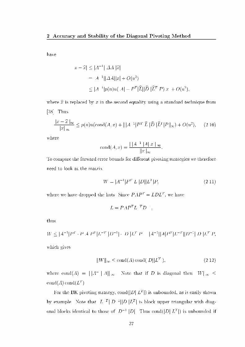
2. Accuracy and Stability of the Diagonal Pivoting Methodhave jx� bxj � jA�1jj�Ajjbxj= jA�1jj�Ajjxj+O(u2)� jA�1jp(n)u(jAj+ P T jbLjj bDjjbLT jP )jxj+O(u2);where bx is replaced by x in the second equality using a standard technique from[58]. Thuskx� bxk1kxk1 � p(n)u(cond(A; x) + kjA�1jP T jbLjj bDjjbLT jPk1) +O(u2); (2.10)where cond(A; x) = kjA�1jjAjjxjk1kxk1 :To compare the forward error bounds for di�erent pivoting strategies we thereforeneed to look at the matrixW = jA�1jP T jLjjDjjLT jP; (2.11)where we have dropped the hats. Since PAP T = LDLT , we haveL = PAP TL�TD�1;thusW � jA�1jP T � P jAjP T jL�T jjD�1j � jDjjLT jP = jA�1jjAjP T jL�T jjD�1jjDjjLT jP;which gives kWk1 � cond(A) cond(jDjjLT j); (2.12)where cond(A) = kjA�1jjAjk1. Note that if D is diagonal then kWk1 �cond(A) cond(LT ).For the BK pivoting strategy, cond(jDjjLT j) is unbounded, as is easily shownby example. Note that jL�T jjD�1jjDjjLT j is block upper triangular with diag-onal blocks identical to those of jD�1jjDj. Thus cond(jDjjLT j) is unbounded if37

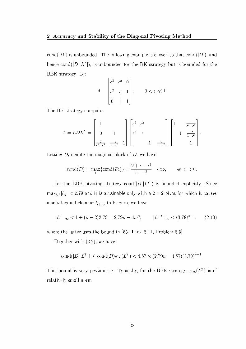
2. Accuracy and Stability of the Diagonal Pivoting Methodcond(jDj) is unbounded. The following example is chosen so that cond(jDj), andhence cond(jDjjLT j), is unbounded for the BK strategy but is bounded for theBBK strategy. Let A = 26664�5 �2 0�2 � 10 1 137775 ; 0 < �� 1:The BK strategy computesA = LDLT = 26664 10 11�2��4 ��1��2 13777526664�5 �2�2 � 1 + �1��237775266641 1�2��41 ��1��21 37775 :Letting Di denote the diagonal block of D, we havecond(D) = maxi fcond(Di)g = 2 + � + �3�� �3 !1; as �! 0:For the BBK pivoting strategy cond(jDjjLT j) is bounded explicitly. Sincemaxi;j jlijj < 2:79 and it is attainable only with a 2� 2 pivot for which it causesa subdiagonal element li+1;i to be zero, we havekLTk1 < 1 + (n� 2)2:79 = 2:79n� 4:57; kL�Tk1 < (3:79)n�1; (2.13)where the latter uses the bound in [55, Thm. 8.11, Problem 8.5].Together with (2.2), we havecond(jDjjLT j) � cond(D)�1(LT ) < 4:57� (2:79n� 4:57)(3:79)n�1:This bound is very pessimistic. Typically, for the BBK strategy, �1(LT ) is ofrelatively small norm.

38

2. Accuracy and Stability of the Diagonal Pivoting Method2.5 The Role of Ashcraft, Grimes and Lewis Ex-ampleAshcraft, Grimes and Lewis [6] have identi�ed a set of matrices for which theBBK strategy achieves better accuracy that the BK strategy. In this section, wegive some explanations for the better accuracy achieved by the BBK strategy,and assess the importance of the examples.We know that the accuracy of the BK algorithm goes hand in hand with illconditioned pivots and unbounded L. The examples of Ashcraft, Grimes andLewis ensure that pivots of cases (2) and (4) of the BK pivoting strategy arechosen and that a large-normed L is formed. However the complicated require-ments of pivot selection within the BK pivoting strategy guarantee cancellationbetween the large and small elements and hence yield the normwise backwardstability result.Experiments similar to those described in Ashcraft, Grimes and Lewis [6] wereperformed. Test matrices are scaled using the scheme described in Figure 2.2 andTable 2.2 in which large entries in L arise. Each set of parameters was given adi�erent random symmetric inde�nite matrix A 2 Rn�n with elements normallydistributed with mean 0 and variance 1. In total 62 test matrices were generated.We chose x as xi = (�1)i and b := Ax. Note that the computed b is not theexact right hand side corresponding to x due to rounding error in its formation.We measure the ratio �1 between the normwise forward errors of BK andBBK �1 = kbx� xk1;BKkbx� xk1;BBK ;and compare with cond(jDjjLT j)BK, the value of cond(jDjjLT j) for BK. Here thesubscripts BK and BBK denote the computed quantities using the BK and BBKstrategies respectively. Our results, which show an increasing trend of �1 and39

2. Accuracy and Stability of the Diagonal Pivoting Methodm n�m�1�2 �1�2 �2 �1... ... ... . . .�2 �2 �2 � � � �1�2 �2 �2 � � � �2 �3�2 �2 �2 � � � �2 1 �3�2 �2 �2 � � � �2 1 1 �3... ... ... ... ... ... ... ... . . .�2 �2 �2 � � � �2 1 1 1 � � � �3Figure 2.2: Scaling parameter for each entry of test matrix.initial pivot �1 �2 �3 t1 t21� 1 pivot 10�t1 10�t2 1=10 t2 + 1; : : : ; 2t2 1; : : : ; 6well-conditioned 2� 2 block 10�t1 10�t2 10�t2 2t2 + 1; : : : ; 3t2 2; : : : ; 6general 2� 2 block 10�t1 10�t2 1=10 2t2 + 1; : : : ; 3t2 1; : : : ; 6Table 2.2: Parameterization of scaled test matrices.cond(jDjjLT j)BK, agree with the test results of Ashcraft, Grimes and Lewis [6];see Figure 2.3. We note that �1 � 1 for several entries, which shows that thescaling scheme sometimes has no e�ect on the accuracy of the computed solution.Recall that if L and D are nonnegative, that is, jLj = L and jDj = D, thenW = jA�1jP T jLjjDjjLT jP = jA�1jjAj, and we have a perfect stability result.The a priori componentwise forward error bound (2.10) involves the quantitykWk1, which may be uninformative. The elements of the Ashcraft, Grimes andLewis examples vary over 18 orders of magnitude, so while kWBKk1=kWBBKk1is small (between orders 100 to 103 for these examples), we may be making largeperturbations in the small elements of jA�1jjAj. Thus a componentwise measure� = minf� : jA�1jP T jLjjDjjLT jP � �jA�1jjAjg (2.14)is employed. Figure 2.4 shows an increasing trend between the ratio �BBK=�BK40

2. Accuracy and Stability of the Diagonal Pivoting Method

102

104

106

108

1010

1012

10−1

100

101

102

103

104

105

106

cond(jDjjLT j)BK� 1

Figure 2.3: Comparison of relative normwise forward error on scaled N(0; 1) matriceswith m = 3, n = 50.and cond(jDjjLT j)BK. Here we use the convention that z=0 = 0 if z = 0 andin�nity otherwise. This brings us back to consider the componentwise backwardstability, where an important measure is � de�ned as in (2.7). If � is smallthen � is more likely to be small. Figure 2.5 shows an increasing trend betweenthe ratio �BK=�BBK and �BK=�BBK. Thus, we can view the Ashcraft, Grimes andLewis examples as a special case for which large a priori componentwise backwardbounds are attained for the BK strategy but not for the BBK strategy. This isbest explained by the following example.LetA = 2666666645:6454e{19 3:0242e{07 7:5198e{07 4:7523e{075:4618e{19 5:7984e{07 3:9042e{079:6075e{02 3:5680e{011:5935e{02

377777775 ; (2.15)which is scaled using the scheme described in Figure 2.2 with m = 2, n = 4,41

2. Accuracy and Stability of the Diagonal Pivoting Method

102

104

106

108

1010

1012

10−1

100

101

102

103

104

105

106

cond(jDjjLT j)BK� BK=� BBK

Figure 2.4: Comparison of relative componentwise forward error bound on scaledN(0; 1) matrices with m = 3, n = 50.

10−1

100

101

102

103

104

105

106

10−1

100

101

102

103

104

105

106

�BK=�BBK� BK=� BBK

Figure 2.5: Comparison of relative componentwise forward error bound on scaledN(0; 1) matrices with m = 3, n = 50. 42

2. Accuracy and Stability of the Diagonal Pivoting Method�1 = 10�18, �2 = 10�6 and �3 = 10�1. For the BK pivoting strategy,P T jLjjDjjLT jP = 2666666645:6454e{19 3:0242e{07 7:5198e{07 4:7523e{071 :3364 e{01 7 :7276 e{02 2 :8698 e{019:6075e{02 3:5680e{018 :0927 e{01

377777775 ;where the italic and underlined entries are those that have changed order com-pared with A. Similarly, for the BBK pivoting strategy, we haveP T jLjjDjjLT jP = 2666666643 :5668 e{12 3:0242e{07 7:5198e{07 4:7523e{072 :2508 e{12 5:7984e{07 3:9042e{079:6075e{02 3:5680e{011:5935e{02

377777775 :For matrix (2.15), �BK=�BBK = 3:0� 1010 and �BK=�BBK = 4:0� 1010. Thus amuch larger componentwise backward error bound is obtained by the BK strategy.In this case, the BBK strategy is superior to the BK strategy.However, from the discussion in Sections 2.4.4 and 2.4.5, we know that neitherthe BK strategy nor the BBK strategy is better than the other from the point ofview of componentwise backward stability in general, and a large kWk1 is onlya necessary condition for componentwise forward instability.2.6 Concluding RemarksWe have investigated the accuracy and stability of the diagonal pivoting methodwith two related pivoting strategies, namely the Bunch{Kaufman pivoting strat-egy and the Bounded Bunch{Kaufman pivoting strategy. Theoretical analysesand numerical examples demonstrate that the claim of superior accuracy of theBBK pivoting strategy is not fully justi�ed.43

2. Accuracy and Stability of the Diagonal Pivoting MethodFor solving linear systems Ax = b, the unbounded factor L arising from theBunch{Kaufman pivoting strategy has no e�ect on the backward stability or thenormwise forward stability. We have con�rmed that better accuracy is achievedby the BBK strategy when tested on the Ashcraft, Grimes and Lewis examples[6]. The signi�cance of these examples is not clear, however. It may be possiblethat a class of numerical examples can be found where BK is more accurate thanBBK. Further work is needed to produce clear statements about the relativeaccuracy of the BK and BBK strategies.

44

Chapter 3Accuracy and Stability ofAasen's Method3.1 IntroductionAnother important direct method for solving dense symmetric inde�nite linearsystems is Aasen's method with partial pivoting [1] which computes an LTLTfactorization of a symmetric matrix A 2 Rn�nPAP T = LTLT ; (3.1)where L is unit lower triangular with �rst column e1 andT = 266666666664

�1 �1�1 �2 �2. . . . . . . . .. . . . . . �n�1�n�1 �n377777777775is tridiagonal. P is a permutation matrix chosen such that jlijj � 1.To solve a linear system Ax = b using the factorization PAP T = LTLT wesolve in turn Lz = P T b; Ty = z; LTw = y; x = Pw: (3.2)The symmetric inde�nite tridiagonal system Ty = z is usually solved inO(n) opsusing Gaussian elimination with partial pivoting. The disregard of symmetry atthis level has little consequence since the overall process is O(n3) ops.45

3. Accuracy and Stability of Aasen's MethodAasen's method with partial pivoting is the only known stable direct methodfor solving symmetric inde�nite linear systems with a guarantee of no more thann2=2 comparisons and a bounded factor L. The operation count of Aasen'smethod with partial pivoting is the same, up to the highest order terms (n3=3 ops), as that of the diagonal pivoting method with the Bunch{Kaufman pivotingstrategy, described in Chapter 2. Despite the advantages, Aasen's method haslargely been neglected for the last decade. Neither LAPACK [2] nor LINPACK[29] has an implementation of Aasen's method. Since 1993, the Visual Numerics,Inc. has included Aasen's method in their IMSL Fortran 90 MP Library [48], [90].In the 1970s, Barwell and George [7] compared the performance of the diagonalpivoting method with the Bunch{Kaufman partial pivoting strategy with that ofAasen's method in unblocked form, on serial computers such as the IBM 360/75and Honeywell 6050. They concluded that the di�erence in performance of thealgorithms, in terms of execution time, is insigni�cant and is compiler dependent.A more recent LAPACK project report [3] compared unblocked and blocked ver-sions of these two algorithms. The authors reported that Aasen's method withpartial pivoting was faster asymptotically in the unblocked case and slower in theblocked case. However, some limitations of the report are explained in [6]:\Unfortunately, this report is somewhat incomplete in that no detailsof the blocked algorithms were given and only factorization timeswere considered. The test codes used are apparently lost. Further,the range of machines is limited and obsolete."In fact the testing was only done on a Cray 2 computer with 1 processor inwhich oating point arithmetic does not utilize a guard digit. It is an openquestion which method is more computationally e�cient in the context of parallelcomputation.To describe Aasen's method it is convenient �rst to describe the Parlett and46

3. Accuracy and Stability of Aasen's MethodReid method; see Section 3.2. The methods are mathematically identical. Aasen'smethod is computationally more e�cient because of its ingenious reordering ofthe tridiagonalization calculation which allows further exploitation of symmetryand structure. We present Aasen's method in Section 3.3.Often the stability of Aasen's method is taken for granted. No backwardstability result exists in the literature. In Section 3.4, we state a backward stabil-ity result of Higham [57] for which the tridiagonal system is solved by Gaussianelimination with partial pivoting.One important practical issue concerning the stability of algorithms is thegrowth factor. We know very little about the behaviour of the growth factor inAasen's method. Direct search methods [53] were employed to search for largegrowth factors and the results are reported in Section 3.5. In Section 3.6, wepresent our conclusions and identify some open problems.3.2 The Parlett and Reid MethodWe now explain how the Parlett and Reid method works. The �rst stage of thealgorithm can be expressed as follows. If the symmetric matrix A 2 Rn�n isnonzero, we can �nd a permutation � so that�A�T = 26664 1 1 n�21 �1 �1 yT1 �1 �2 vTn�2 y v B 37775;with �1 the largest subdiagonal element in absolute value in the �rst column. If�1 = 0 then no modi�cation is needed and we proceed to the next stage. For �1

47

3. Accuracy and Stability of Aasen's Methodnonzero, we can factorize�A�T = 2666410 10 w In�23777526664�1 �1 0�1 �2 vT � �2wT0 v � �2w C 37775266641 0 01 wTIn�2

37775 ;where w = y=�1 and C = B � wvT � vwT + �2wwT . The process is repeatedrecursively on the (n� 1)� (n� 1) submatrixS = 24 �2 vT � wTv � w C 35 ;yielding the factorization (3.1) on completion. This factorization costs 2n3=3 op-erations (twice the cost as block LDLT factorization with the Bunch{Kaufmanpivoting strategy) plus n2=2 comparisons. Hence Parlett and Reid's method isuncompetitive with the block LDLT factorization with the Bunch{Kaufman piv-oting strategy mentioned in Chapter 2. In next section, we explain how Aasen'smethod exploits symmetry and hence halves the cost of the factorization.3.3 Aasen's MethodFor convenience, we assume, without loss of generality, that no interchanges areneeded, which amounts to rede�ning A := PAP T in (3.1). To derive Aasen'smethod, assume that the �rst i� 1 columns of T and the �rst i columns of L areknown. We show how to compute the ith column of T and the (i + 1)st columnof L. A key role is played by the matrixH = TLT ; (3.3)48

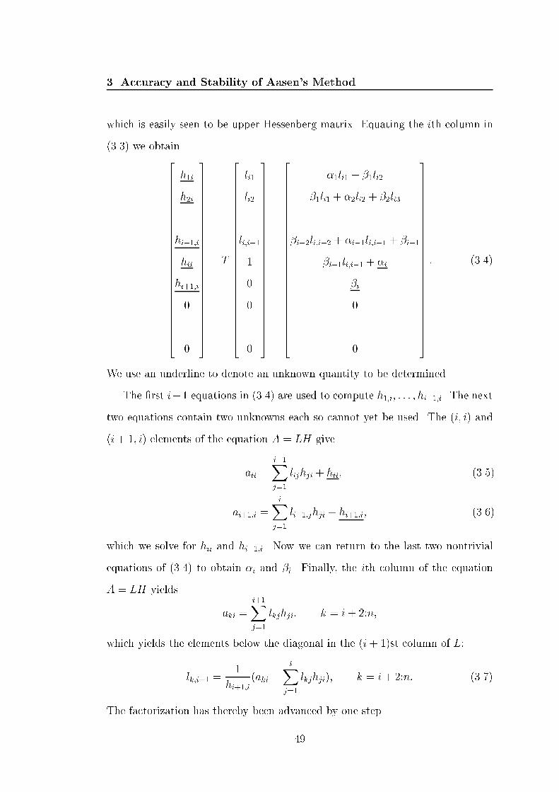
3. Accuracy and Stability of Aasen's Methodwhich is easily seen to be upper Hessenberg matrix. Equating the ith column in(3.3) we obtain2666666666666666666666664

h1ih2i...hi�1;ihiihi+1;i0...0

3777777777777777777777775= T

2666666666666666666666664

li1li2...li;i�1100...0

3777777777777777777777775=2666666666666666666666664

�1li1 + �1li2�1li1 + �2li2 + �2li3...�i�2li;i�2 + �i�1li;i�1 + �i�1�i�1li;i�1 + �i�i0...0

3777777777777777777777775: (3.4)

We use an underline to denote an unknown quantity to be determined.The �rst i�1 equations in (3.4) are used to compute h1;i; : : : ; hi�1;i. The nexttwo equations contain two unknowns each so cannot yet be used. The (i; i) and(i+ 1; i) elements of the equation A = LH giveaii = i�1Xj=1 lijhji + hii; (3.5)ai+1;i = iXj=1 li+1;jhji + hi+1;i; (3.6)which we solve for hii and hi+1;i. Now we can return to the last two nontrivialequations of (3.4) to obtain �i and �i. Finally, the ith column of the equationA = LH yields aki = i+1Xj=1 lkjhji; k = i + 2:n;which yields the elements below the diagonal in the (i + 1)st column of L:lk;i+1 = 1hi+1;i (aki � iXj=1 lkjhji); k = i+ 2:n: (3.7)The factorization has thereby been advanced by one step.49

3. Accuracy and Stability of Aasen's MethodClearly, equations (3.2), (3.4){(3.6) are allO(n2) ops processes. To derive theleading order of the operation cost, we need only to consider the most expensiveloop (3.7). For each lk;i+1, it costs 2i+ 1 ops. Hence the (i+ 1)st column costs(n� i� 2)(2i+ 1) ops in total. In completion of L we needn�2Xi=1 (n� i� 2)(2i+ 1) = 2 n�2Xi=1 (ni� i2) +O(n2) = n33 +O(n2) ops:3.4 Numerical StabilityOur model of oating point arithmetic is the usual model (1.2). The followingbackward stability result is proved by Higham [57].Theorem 3.4.1 (Higham) Let A 2 Rn�n be symmetric and let bx be a computedsolution to the linear system Ax = b produced by Aasen's method with partialpivoting. Then(A +�A)bx = b; j�Aj � 3n+1P T jbLjjbT jjbLT jP + 2n+4P T jbLj�T jcM jjbU jjbLT jP;where � bT � cM bU and PAP T � bLbT bLT are the computed factorizations producedby LU factorization with partial pivoting and LTLT factorization with partialpivoting respectively. Moreoverk�Ak1 � (n� 1)2 15n+25kbTk1: 2Theorem 3.4.1 shows that Aasen's method is a backward stable method forsolving Ax = b provided that the growth factor�n(A) = maxi;j jtijjmaxi;j jaijj (3.8)is not too large. Here, we are making the reasonable assumption that maxi;j jtijj �maxi;j jbtijj [55, p.177]. 50

3. Accuracy and Stability of Aasen's Method3.5 The Growth FactorIn this section, we bound the growth factor for Aasen's method with partialpivoting and investigate whether the bound is attainable using a combination ofdirect search methods described in [28], [53], [86], [87].First we bound the growth factor. Using the fact that the multipliers inAasen's method with partial pivoting are bounded by 1, it is straightforward toshow that if maxi;j jaijj = 1 then T has a bound illustrated for n = 5 byjT j � 266666666664

1 11 1 22 4 88 16 3232 64377777777775 :Hence �n(A) � 4n�2:This upper bound is attainable for n = 3, as is shown by the exampleA = 26664 1 �1 1�1 1 11 1 137775 = 2666410 10 �1 13777526664 1 �1�1 1 22 437775266641 0 01 �11 37775 = LTLT : (3.9)For n � 4, we were unable to construct such an example. It is an open questionwhether this upper bound is attainable.One useful approach to investigate the numerical instability of an algorithmis to rephrase the question as an optimization problem and apply a direct searchmethod.In our case, the growth factor is expressed as a function f : Rn ! R. Toobtain an optimization problem we let x = vec(A) 2 R(n2+n)=2, where vec(A)comprises the columns of the upper triangular part of A strung out into one long51

3. Accuracy and Stability of Aasen's Methodvector, and we de�ne f(x) = �n(A) where �n(A) is de�ned in (3.8). Then wewish to determine maxx2R(n2+n)=2 f(x) � maxA=AT2Rn�n �n(A): (3.10)Direct search methods are usually based on heuristics that do not involve as-sumptions about the function f . Only function values are used and no derivativeestimate of f is required. The main disadvantages are that the convergence is atbest linear and the nature of the point at which the methods terminate is notknown since derivatives are not calculated [53]. Nevertheless it provides a conve-nient starting point in tackling the problem when limited information is knownabout f .We have used three direct search methods implemented in the Matlab TestMatrix Toolbox [54]. They are the alternating directions method (adsmax.m)[53], the multidirectional search method (mdsmax.m) of Dennis and Torczon [86],[87], and the Nelder-Mead simplex method (nmsmax.m) [28].For our optimization problem (3.10) with n = 3, starting naively with initialmatrix A = I and default tolerance 10�3, mdsmax.m needed only 8 iterations and139 function evaluations to converge. It gave �n(A) = 3:9944, whereA = 26664�0:6370 �0:0835 �0:0835�0:0835 1:0000 �0:9972�0:0835 �0:9972 1:0000 37775is a di�erent form of matrix than our example (3.9).In our remaining experiments, we started the search with a random vectorwith default tolerance which is set to 10�3 for all three routines. When one ofthem converged, we restarted the search using a di�erent method until all threeof them converged to the given tolerance. Then the search was restarted with asmaller tolerance. The tolerance was reduced gradually to 10�15.52

3. Accuracy and Stability of Aasen's MethodFor n = 4 and 5, the largest growth factors found so far are 7:99 and 14:61respectively, compared with the bounds of 16 and 64. It is an open question todetermine a sharp bound for the growth factor. However, unsuccessful optimiza-tions can also provide useful information. As Miller and Spooner explain [66,p. 370],\Failure of the maximizer to �nd large values of ! (say) can be inter-preted as providing evidence for stability equivalent to a large amountof practical experience with low-order matrices."3.6 Concluding RemarksAasen's method is the only stable direct method with O(n2=2) comparisons and abounded factor L, for solving symmetric inde�nite linear system Ax = b. The di-agonal pivoting method with the Bunch{Kaufman pivoting strategy and Aasen'smethod are competitive in terms of speed for dense matrices. It is not clear whichmethod is more e�cient for sparse matrices and on parallel architectures. Moretesting on a wider range of machines is desirable.An open problem is to construct matrices for which the growth factor boundis attained for n � 4, or to derive a sharper growth factor bound for Aasen'smethod.

53

Chapter 4Modi�ed Cholesky Algorithms4.1 IntroductionA standard method for solving unconstrained optimization problems is Newton'smethod. Given a twice continuously di�erentiable function F (x) : Rn ! R, let�rst and second derivatives of F (x) be known at the iterate x(k). A local quadraticmodel of F (x) can be obtained using the �rst three terms of Taylor's series atx(k), that is, F (x(k) + p) � F (k) + g(k)Tp+ 12pTG(k)p;where F (k) = F (x(k)), g(k) = � @F@xi �x=x(k) = rF jx=x(k) is the gradient of F at x(k),G(k) = � @2F@xi@xj �x=x(k) is the Hessian matrix and p is the search direction. Theminimum of the quadratic model is attained when g(k)Tp+ 12pTG(k)p is minimized.For a stationary point, we have r(g(k)Tp+ 12pTG(k)p) = 0, which givesG(k)bp = �g(k): (4.1)The search direction bp satisfying (4.1) is called the Newton direction and theminimization algorithm that takes a unit step in this direction at each stage isNewton's method. In practice, a line search is incorporated, that is, x(k+1) =x(k)+�kbp is used instead, where �k is chosen so that F (x(k)+�kbp) is minimized.If G(k) is positive de�nite, a descent direction bp is guaranteed since g(k)T bp =�g(k)T (G(k))�1g(k) < 0. In practice, we want g(k)T bp < ��, for some positiveconstant �, so that F can be \su�ciently reduced" for small enough �k, whichis essential to achieve convergence [36]. In any case, if bp satis�es some modi�edversion of (4.1), we called the algorithm a modi�ed Newton method.54

4. Modi�ed Cholesky AlgorithmsGiven an inde�nite Hessian matrix, one popular approach is to compute a\nearby" positive de�nite matrix to the original inde�nite one. A natural ap-proach is to combine a matrix factorization like the Cholesky (LDLT) factor-ization with a modi�cation scheme. This widely used technique is the so-calledmodi�ed Cholesky factorization [37], [78]. In this chapter, we describe the two ex-isting modi�ed Cholesky factorizations and propose two alternative modi�cationschemes.Given a symmetric matrix and not necessarily positive de�nite matrix A,a modi�ed Cholesky algorithm produces a symmetric perturbation E such thatA+E is positive de�nite, along with a Cholesky (or LDLT) factorization of A+E.The objectives of a modi�ed Cholesky algorithm can be stated as follows [78].O1. If A is \su�ciently positive de�nite" then E should be zero.O2. If A is inde�nite, kEk should not be much larger thanminf k�Ak : A+�A is positive de�nite g ;for some appropriate norm.O3. The matrix A + E should be reasonably well conditioned.O4. The cost of the algorithm should be the same as the cost of standardCholesky factorization to highest order terms.Two existing modi�ed Cholesky algorithms are one of Gill, Murray and Wright(the GMW algorithm) [37, Section 4.4.2.2], which is a re�nement of an earlieralgorithm of Gill and Murray [36], and an algorithm of Schnabel and Eskow (theSE algorithm) [78].We explain the GMW and SE algorithms in Sections 4.2 and 4.3 respectively.The GMW and SE algorithms both increase the diagonal entries as necessary inorder to ensure that negative pivots are avoided. Hence both algorithms produce55

4. Modi�ed Cholesky AlgorithmsCholesky factors of P (A + E)P with a diagonal E, where P is a permutationmatrix.In Section 4.4, we show that the \optimal" perturbation in objective (O2) is,in general, full for the Frobenius norm and can be taken to be diagonal for the2-norm (but is generally not unique). There seems to be no particular advantageto making a diagonal perturbation to A. We propose an alternative modi�edCholesky algorithm based on the block LDLT factorization with the boundedBunch{Kaufman (BBK) pivoting strategy described in Chapter 2. Our algorithmperturbs the whole matrix, in general. However, it is suitable even for sparsematrices since our proposed modi�cation scheme keeps the sparsity of the factorsL and D.In outline, our approach is to compute a block LDLT factorizationPAP T = LDLT ; (4.2)where P is a permutation matrix, L is unit lower triangular and D is blockdiagonal with diagonal blocks of dimension 1 or 2, and to provide the factorizationP (A+ E)P T = L(D + F )LT ;where F is chosen so that D + F (and hence also A+ E) is positive de�nite.This approach is not new; it was suggested by Mor�e and Sorensen [67] foruse with the block LDLT factorization computed with the Bunch{Kaufman [12]and Bunch{Parlett [14] pivoting strategies. However, for neither of these pivotingstrategies are all the conditions (O1){(O4) satis�ed, as is recognized in [67]. TheBunch{Parlett pivoting strategy requires O(n3) comparisons for an n�n matrix,so condition (O4) does not hold. For the Bunch{Kaufman strategy, which requiresonly O(n2) comparisons, it is di�cult to satisfy conditions (O1){(O3), as weexplain in Section 4.4.There are two reasons why our algorithm might be preferred to those of Gill,Murray and Wright, and of Schnabel and Eskow. The �rst is a pragmatic one: we56

4. Modi�ed Cholesky Algorithmscan make use of any available implementation of the form (4.2), needing to addjust a small amount of post-processing code to form the modi�ed factorization.In particular, we can use the e�cient implementations for both dense and sparsematrices written by Ashcraft, Grimes and Lewis [6], which make extensive use oflevel 2 and 3 BLAS for e�ciency on high-performance machines. In contrast, incoding the GMW and SE algorithms one must either begin from scratch or makenon-trivial changes to an existing Cholesky factorization code.The second attraction of our approach is that we have a priori bounds thatexplain the extent to which conditions (O1){(O3) are satis�ed|essentially, if Lis well conditioned then an excellent modi�ed factorization is guaranteed. Forthe GMW and SE algorithms it is di�cult to describe under what circumstancesthe algorithms can be guaranteed to perform well.Note that the analysis in Section 4.4 works for all congruence transformations.In Section 4.5 we describe a modi�ed Aasen algorithm based on Aasen's method.Numerical results are presented in Section 4.7. We give conclusions and directionsfor future work in Section 4.8.4.2 The Gill, Murray and Wright AlgorithmIn this section, we summarize the algorithm of Gill, Murray and Wright (theGMW algorithm) [37], which is designed to satisfy the four objectives statedin Section 4.1. The GWM algorithm is based on the LDLT factorization (orthe Cholesky factorization) and modi�es only diagonal elements, that is, givenA 2 Rn�n , we compute PAP T + E = L bDLT ; (4.3)57

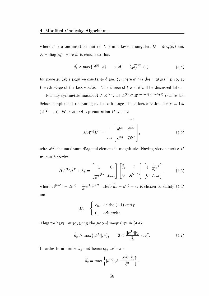
4. Modi�ed Cholesky Algorithmswhere P is a permutation matrix, L is unit lower triangular, bD = diag(bdi) andE = diag(ei). Here bdi is chosen so thatbdi � maxfjd(i)j; �g and lij bd 1=2j � �; (4.4)for some suitable positive constants � and �, where d(i) is the \natural" pivot atthe ith stage of the factorization. The choice of � and � will be discussed later.For any symmetric matrix A 2 Rn�n , let A(k) 2 R(n�k+1)�(n�k+1) denote theSchur complement remaining at the kth stage of the factorization, for k = 1:n(A(1) = A). We can �nd a permutation � so that�A(k)�T = 264 1 n�k1 d(k) c(k)Tn�k c(k) B(k) 375; (4.5)with d(k) the maximum diagonal element in magnitude. Having chosen such a �we can factorize�A(k)�T + Ek = 24 1 01bdk c(k) In�k3524bdk 00 A(k+1)35241 1bdk cT0 In�k35 ; (4.6)where A(k+1) = B(k) � 1bdk c(k)c(k)T . Here bdk = d(k) + ek is chosen to satisfy (4.4)and Ek = 8<: ek; at the (1,1) entry,0; otherwise.Thus we have, on squaring the second inequality in (4.4),bdk � maxfjd(k)j; �g; 0 � kc(k)k21bdk � �2: (4.7)In order to minimize bdk and hence ek, we havebdk = max�jd(k)j; �; kc(k)k21�2 � :58

4. Modi�ed Cholesky AlgorithmsHence jekj = jbdk � d(k)j � max�jd(k)j; �; kc(k)k21�2 �+ jd(k)j� kc(k)k21�2 + 2jd(k)j+ �: (4.8)This process is repeated recursively on the Schur complement A(k+1) yielding thefactorization (4.3) on completion.Gill and Murray [36] derive an upper bound for kE(�)k2, depending on �,using the following lemma.Lemma 4.2.1 (Gill and Murray) Let A 2 Rn�n and � be de�ned as in (4:4).Let A(k) denote the Schur complement at the kth stage of the GMW algorithm.We have ja(k)ii j � � + (k � 1)�2; ja(k)ij j � � + (k � 1)�2; i 6= j; (4.9)where � = maxi jaiij and � = maxi6=j jaijj.Proof: The proof is by induction. For k = 1, (4.9) is trivially true sinceA(1) = A. Assume (4.9) is true for k = m. For k = m + 1, using the secondinequality in (4.7), we haveja(m+1)ii j � jb(m)ii j+ jbd�1m (c(m)i )2j � � +m�2;ja(m+1)ij j � jb(m)ij j+ jbd�1m c(m)i c(m)j j � � +m�2;as required. 2Using Lemma 4.2.1 and (4.8), it is easily shown thatkE(�)k2 = maxi jeij � ��� + (n� 1)��2 + 2�� + (n� 1)�2�+ �: (4.10)It remains to describe the choice of � and �. For �, note that the bound ofkE(�)k2 is a convex function of � and is minimized when �2 = �=pn2 � 1 [36].59

4. Modi�ed Cholesky AlgorithmsIn addition, a lower bound for � is required so that objective (O1) is satis�ed,that is, kE(�)k2 = 0 when A is su�ciently positive de�nite. When no modi�ca-tion is added, the GMW algorithm is just the standard LDLT factorization withcomplete pivoting and aii =Pij=1 l2ijdj with dj > 0. This implies0 < l2ijdj � aii � maxk akk = �:If � � �2, (4.4) guarantees no modi�cation is made. So the �nal choice of � is�2 = maxf�; �=pn2 � 1; ug;where u is the unit roundo� and is introduced to allow for the case when A = 0.No detail of how � is chosen is given in [37]. The default value of � in MargaretWright's Matlab code for the GMW algorithm is � = 2umaxf� + �; 1g.At each stage, kc(k)k1 is computed to determine the amount of perturbation,hence the extra cost induced is n2=2 to the highest order. The cost of the pivotingis also n2=2 to the highest order. Thus objective (O4) is trivially satis�ed.4.3 The Schnabel and Eskow AlgorithmThe algorithm of Schnabel and Eskow (the SE algorithm) is broadly similar tothe GMW algorithm. The SE algorithm also carries out the LDLT factorizationusing the Gershgorin circle theorem to determine the size of the perturbationand the choice of pivot, and has a two-phase strategy. Given A 2 Rn�n , the SEalgorithm computes PAP T + E = L bDLT ;where P is a permutation matrix, L is unit lower triangular, bD = diag(bdi) andE = diag(ei).The two-phase strategy is used to avoid perturbing su�ciently positive-de�nitematrices. In the �rst phase, the LDLT factorization with complete pivoting (that60

4. Modi�ed Cholesky Algorithmsis, pivoting along the diagonal) is used. We switch to the second phase of thealgorithm if the minimum diagonal element in the Schur complement is smallerthan �, where � = �� and � = u1=3 is recommended in [78].No modi�cation is made in the �rst phase and the element growth is boundedusing the following lemma (cf. Schnabel and Eskow [78, Thm. 5.2.1]).Lemma 4.3.1 Let A 2 Rn�n and let � be a positive constant. Let the �rst phaseof the SE algorithm be completed at the end of the (k � 1)st stage and switch tothe second phase at the kth stage. Let A(k) 2 R(n�k+1)�(n�k+1) denote the Schurcomplement. If mink�i�n a(k)ii � �, thena(k)ii � �; ja(k)ij j � � + � � �; i 6= j; (4.11)where � = maxi jaiij and � = maxi6=j jaijj.Proof: At the end of the (k � 1)st stage, we have�A�T = 24 k�1 n�k+1k�1 H CTn�k+1 C B 35 = 24L 0M In�k+13524D 00 A(k)3524LT MT0 In�k+135 ;which gives B =MDMT + A(k):This implies, for i = k:n,� � bii = k�1Xj=1 m2ijdj + a(k)ii > �;thus a(k)ii � � and Pk�1j=1 m2ijdj � � � �. Moreover, using the Cauchy{Schwartzinequality, we haveja(k)ij j � jbijj+ ��� k�1Xr=1 mirdrmrj���� jbijj+ � k�1Xr=1 m2irdr�12� k�1Xr=1 m2jrdr� 12� � + �� �; 61

4. Modi�ed Cholesky Algorithmswhich completes the proof. 2If the �rst phase runs to completion, then the SE algorithm performs an LDLTfactorization with complete pivoting. The SE algorithm switches to the secondphase at the kth stage if mink+1�i�n a(k+1)ii < �.Once the algorithm switches to the second phase, the Gershgorin circle theo-rem is used to determine the amount of perturbation and the choice of pivot.Theorem 4.3.2 (Gershgorin Circle Theorem) Let A 2 C n�n . Then eacheigenvalue �i of A lies in one of the disks in the complex planeGi = (�i : j�i � aiij �Xj 6=i jaijj) ; i = 1:n:Proof: See [81]. 2For a real symmetric matrix, Theorem 4.3.2 says that all the eigenvalues liein a union of real intervals fG1 [ � � � [Gng, whereGi = [gi�; gi+] := "aii �Xi6=j jaijj; aii +Xi6=j jaijj# : (4.12)Let A(k) 2 R(n�k+1)�(n�k+1) denote the Schur complement of the kth stageof the factorization and have the Gershgorin intervals G(k)i , i = k:n, de�ned asin (4:12). Schnabel and Eskow [78] determine their choice of perturbation sothat the Gershgorin intervals contract at each step of the factorization, that is,G(k+1)i � G(k)i , i = k + 1:n. The following lemma is a modi�ed version of [78,Lem. 5.1.1] in which we have introduced a positive tolerance �. Recall that ifA(k) = 24 1 n�k1 d(k) c(k)Tn�k c(k) B(k) 35;then A(k+1) = B(k)� 1bdk c(k)c(k)T where bdk = d(k)+ ek is chosen to satisfy (4.13) inthe following lemma. 62

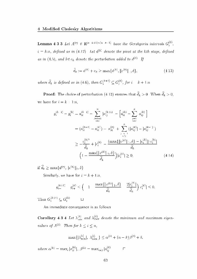
4. Modi�ed Cholesky AlgorithmsLemma 4.3.3 Let A(k) 2 R(n�k+1)�(n�k+1) have the Gershgorin intervals G(k)i ,i = k:n, de�ned as in (4:12). Let d(k) denote the pivot at the kth stage, de�nedas in (4:5), and let ek denote the perturbation added to d(k). Ifbdk := d(k) + ek � maxfd(k); kc(k)k1; �g; (4.13)where bdk is de�ned as in (4:6), then G(k+1)i � G(k)i , for i = k + 1:n.Proof: The choice of perturbation (4.13) ensures that bdk > 0. When bdk > 0,we have for i = k + 1:n,g(k+1)i� � g(k)i� = a(k+1)ii � nXj=k+1i6=j ja(k+1)ij j � ha(k)ii � nXj=ki6=j ja(k)ij ji= (a(k+1)ii � a(k)ii ) + ja(k)ik j+ nXj=k+1i6=j (ja(k)ij j � ja(k+1)ij j)� �c(k)2ibdk + jc(k)i j � (maxfkc(k)k1; �g � jc(k)i j)jc(k)i jbdk= �1� maxfkc(k)k1; �gbdk �jc(k)i j � 0; (4.14)if bdk � maxfd(k); kc(k)k1; �g.Similarly, we have for i = k + 1:n,g(k+1)i+ � g(k)i+ � �� 1 + maxfkc(k)k1; �gbdk � 2jc(k)i jbdk �jc(k)i j � 0:Thus G(k+1)i � G(k)i . 2An immediate consequence is as follows.Corollary 4.3.4 Let �(k)min and �(k)max denote the minimum and maximum eigen-values of A(k). Then for k � i � n,maxfj�(i)minj; j�(i)maxjg � �(k) + (n� k)�(k) + �;where �(k) = maxi ja(k)ii j, �(k) = maxi6=j ja(k)ij j. 263

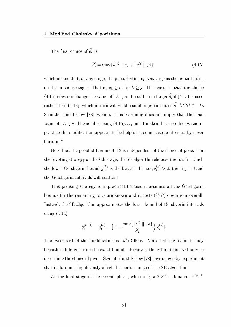
4. Modi�ed Cholesky AlgorithmsThe �nal choice of bdi isbdi = maxfd(i) + ei�1; kc(i)k1; �g; (4.15)which means that, at any stage, the perturbation ei is as large as the perturbationon the previous stages. That is, ek � ej for k � j. The reason is that the choice(4.15) does not change the value of kEk2 and results in a larger bdi if (4.15) is usedrather than (4.13), which in turn will yield a smaller perturbation bd�1i c(i)c(i)T . AsSchnabel and Eskow [78] explain, \this reasoning does not imply that the �nalvalue of kEk2 will be smaller using (4.15): : : , but it makes this seem likely, and inpractice the modi�cation appears to be helpful in some cases and virtually neverharmful."Note that the proof of Lemma 4.3.3 is independent of the choice of pivot. Forthe pivoting strategy at the kth stage, the SE algorithm chooses the row for whichthe lower Gershgorin bound g(k)i� is the largest. If maxi g(k)i� > 0, then ek = 0 andthe Gershgorin intervals will contract.This pivoting strategy is impractical because it assumes all the Gershgorinbounds for the remaining rows are known and it costs O(n3) operations overall.Instead, the SE algorithm approximates the lower bound of Gershgorin intervalsusing (4.14) g(k+1)i� = g(k)i� + �1� maxfkc(k)k1; �gbdk �jc(k)i j:The extra cost of the modi�cation is 5n2=2 ops. Note that the estimate maybe rather di�erent from the exact bounds. However, the estimate is used only todetermine the choice of pivot. Schnabel and Eskow [78] have shown by experimentthat it does not signi�cantly a�ect the performance of the SE algorithm.At the �nal stage of the second phase, when only a 2 � 2 submatrix A(n�1)64

4. Modi�ed Cholesky Algorithmsremains, we chooseen�1 = bdn�1 � d(n�1)= max(en�2;��(n�1)min +maxn�(�(n�1)max � �(n�1)min )1� � ; �o)� max(en�2; j�(n�1)min j+ �(j�(n�1)max j+ j�(n�1)min j)1� � + �) ;where �(n�1)max and �(n�1)min denote the maximum and minimum eigenvalues of A(n�1)respectively.Suppose the SE algorithm switches to the second phase at the bkth stage.Using Lemma 4.3.1 and Corollary 4.3.4, we havekEk2 � 1 + �1� � h�(bk) + (n� bk)�(bk) + �i+ �� 1 + �1� � h�+ (n� bk)(� + �� �)i+ 21� � �� 1 + �1� � [n(� + �)] + 21� � �; (4.16)which is a smaller bound than that of the Gill, Murray and Wright algorithmde�ned as in (4.10) by a factor n.4.4 The New Modi�ed Cholesky AlgorithmWe begin by de�ning the distance from a symmetric matrix A 2 Rn�n to thesymmetric matrices with minimum eigenvalue �min at least �, where � � 0:�(A; �) = minfk�Ak : �min(A+�A) � �g : (4.17)The distance in the 2- and Frobenius norms, and perturbations that achieve themare easily evaluated (see Halmos [47], Higham [51, Thms. 2.1, 3.1]).65

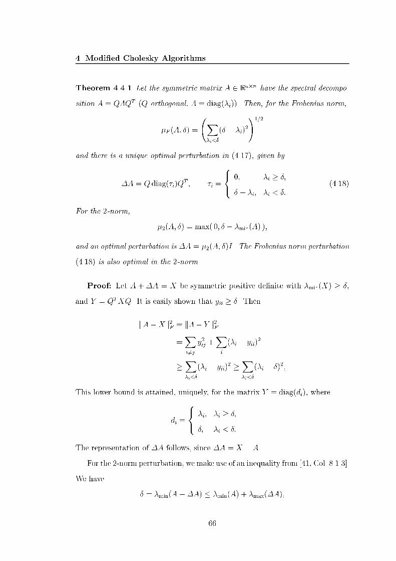
4. Modi�ed Cholesky AlgorithmsTheorem 4.4.1 Let the symmetric matrix A 2 Rn�n have the spectral decompo-sition A = Q�QT (Q orthogonal, � = diag(�i)). Then, for the Frobenius norm,�F (A; �) = X�i<�(� � �i)2!1=2and there is a unique optimal perturbation in (4.17), given by�A = Q diag(�i)QT ; �i = 8<: 0; �i � �;� � �i; �i < �: (4.18)For the 2-norm, �2(A; �) = max( 0; � � �min(A) );and an optimal perturbation is �A = �2(A; �)I. The Frobenius norm perturbation(4.18) is also optimal in the 2-norm.Proof: Let A +�A = X be symmetric positive de�nite with �min(X) � �,and Y = QTXQ. It is easily shown that yii � �. ThenkA�Xk2F = k�� Y k2F=Xi6=j y2ij +Xi (�i � yii)2�X�i<�(�i � yii)2 �X�i<�(�i � �)2;This lower bound is attained, uniquely, for the matrix Y = diag(di), wheredi = 8<: �i; �i � �;�; �i < �:The representation of �A follows, since �A = X � A.For the 2-norm perturbation, we make use of an inequality from [41, Col. 8.1.3].We have � = �min(A+�A) � �min(A) + �max(�A);66

4. Modi�ed Cholesky Algorithmswhere A, �A are symmetric. The equality is achieved when �max(�A) = � ��min(A), hence the result.By taking the 2-norm of the perturbation, it is trivial to show that the optimalFrobenius norm perturbation is also an optimal 2-norm perturbation. 2Our modi�ed Cholesky algorithm has a parameter � � 0 and it attempts toproduce the perturbation (4.18).AlgorithmMC (Modi�ed Cholesky Factorization) Given a symmetric ma-trix A 2 Rn�n and a parameter � � 0 this algorithm computes a permutationmatrix P , a unit lower triangular matrix L, and a block diagonal matrix D withdiagonal blocks of dimension 1 or 2, such thatP (A+ E)P T = LDLTand A + E is symmetric positive de�nite (or symmetric positive semide�nite if� = 0). The algorithm attempts to ensure that if �min < � then �min(A+E) � �.1. Compute the symmetric inde�nite factorization PAP T = L eDLT using theBBK pivoting strategy (Algorithm BBK).2. Let D = eD+� eD, where � eD is the minimum Frobenius norm perturbationthat achieves �min( eD+� eD) � � (thus � eD = diag(� eDii), where � eDii is theminimumFrobenius norm perturbation that achieves �min( eDii+� eDii) � �).To what extent does Algorithm MC achieve the objectives (O1){(O4) listedin Section 4.1? Objective (O4) is clearly satis�ed, provided that the pivotingstrategy does not require a large amount of searching, since the cost of step 2 isnegligible. For objectives (O1){(O3) to be satis�ed we need the eigenvalues ofA to be reasonably well approximated by those of eD. For the Bunch{Kaufmanpivoting strategy the elements of L are unbounded and the eigenvalues of eD candi�er greatly from those of A (subject to A and eD have the same inertia), as is67

4. Modi�ed Cholesky Algorithms�(A) �( eDBBK) �( eDBK)�6:1e�01 �1:0e+00 �1:0e�051.0e�10 1.0e�10 1.0e�051:6e+00 1.0e+00 1.0e+00Table 4.1: The eigenvalues of matrix (4.19) and the block diagonal matrix eD when theBBK and BK pivoting strategies are used.easily shown by example. Let A = 266640 � 0� 0 10 1 137775 ; (4.19)where � = 10�5. Table 4.1 displays the eigenvalues of A and of the block diago-nal eD computed using the LDLT factorization with the BK and BBK strategies(denoted by eDBK and eDBBK respectively). The eigenvalues of eDBK di�er as muchas an order of 5 from those of A. This is the essential reason why the Bunch{Kaufman pivoting strategy is unsuitable for use in a modi�ed Cholesky algorithm.To investigate objectives (O1){(O3) we will make use of a theorem of Os-trowski [60, p. 224], [69]. Here the eigenvalues of a symmetric n � n matrix areordered such that �1 � � � � � �n.Theorem 4.4.2 (Ostrowski) Let M 2 Rn�n be symmetric and S 2 Rn�n non-singular. Then for each k, k = 1:n,�k(SMST ) = �k�k(M)where �1(SST ) � �k � �n(SST ). 2Note that the Sylvester law of inertia [41, Thm. 8.1.12] is a corollary of Ostrowski'stheorem. 68

4. Modi�ed Cholesky AlgorithmsAssuming �rst �min(A) > 0, and applying the theorem with M = eD andS = L, we obtain �min(A) � �max(LLT )�min( eD):Now E will be zero if �min( eD) � �, which is certainly true if�min(A) � ��max(LLT ): (4.20)Next we assume that �min(A) is negative and apply Theorem 4.4.1 and The-orem 4.4.2 to obtain�max(� eD) = � � �min( eD) � � � �min(A)�min(LLT ) : (4.21)Using Theorem 4.4.2 again, with (4.21), yieldskEk2 = �max(E) = �max(L eDLT )� �max(LLT )�max( eD)� �max(LLT )�� � �min(A)�min(LLT )� ; (4.22)where �min(A) < 0. A �nal invocation of Theorem 4.4.2 gives�min(A+ E) � �min(LLT )�min( eD +� eD) � �min(LLT )�:and kA+ Ek2 = �max(A+ E) = �max(L( eD +� eD)LT )� �max(LLT )�max( eD +� eD)= �max(LLT )maxf�; �max( eD)g� �max(LLT )max��; �max(A)�min(LLT )� :Hence �2(A+ E) � �2(LLT )max�1; �max(A)�min(LLT )�� : (4.23)69

4. Modi�ed Cholesky AlgorithmsWe can now assess how well objectives (O1){(O3) are satis�ed. To satis�edobjective (O1) we would like E to be zero when �min � �, and to satisfy (O2)we would like kEk2 to be not much larger than � � �min when A is not positivede�nite. The su�cient condition (4.20) for E to be zero and inequality (4.22)show that these conditions do hold modulo factors �max;min(LLT ). Inequality(4.23) bounds �2(A + E) with the expected reciprocal dependence on �, againwith terms �max;min(LLT ). The conclusion is that Algorithm MC is guaranteedto perform well if �min(LLT ) and �max(LLT ) are not too far from 1.Note that, since L is unit lower triangular, eT1 (LLT )e1 = 1, which implies that�min(LLT ) � 1 and �max(LLT ) � 1. For the BBK pivoting strategy we havemaxi;j jlijj � 2:781, so1 � �max(LLT ) � trace(LLT ) = kLk2F � n+ 12n(n� 1)2:7812 � 4n2 � 3n:(4.24)Furthermore,1 � �min(LLT )�1 � k(LLT )�1k2 � kL�1k22 � (3:781)2n�2; (4.25)using a bound from [55, Thm. 8.13 and Problem 8.5]. These upper bounds areapproximately attainable, but in practice are rarely approached. In particular,the upper bound of (4.25) can be approached only in the unlikely event that mostof the subdiagonal elements of L are negative and of near maximal magnitude.Note that each 2� 2 pivot causes a subdiagonal element li+1;i to be zero and sofurther reduces the likelihood of kL�1k2 being large.The modi�ed Cholesky algorithm in this section and the corresponding anal-ysis are not tied exclusively to the BBK pivoting strategy. We could use insteadthe \fast Bunch{Parlett" pivoting strategy from [6], which appears to be moree�cient than the BBK pivoting strategy when both are implemented in blockform [6]. 70

4. Modi�ed Cholesky Algorithms4.5 The Modi�ed Aasen AlgorithmIn this section, we assess the feasibility of using LTLT factorization with partialpivoting for computing a modi�ed factorization. Our modi�ed Aasen algorithmhas a parameter � � 0 and it attempts to produce the perturbation (4.18).Algorithm MA (Modi�ed Aasen Factorization) Given a symmetric matrixA 2 Rn�n and a parameter � � 0 this algorithm computes a permutation matrixP , a unit lower triangular matrix L, and a full matrix T such thatP (A+ E)P T = LTLTand A + E is symmetric positive de�nite (or symmetric positive semide�nite if� = 0). The algorithm attempts to ensure that if �min < � then �min(A+E) � �.1. Compute the factorization PAP T = LeTLT using Aasen's method.2. Let T = eT +�eT , where �eT is the minimum Frobenius norm perturbationthat achieves �min(eT +�eT ) � �.Since equalities (4.20){(4.23) do not depend on the fact that eD is block di-agonal, it is obvious that the discussion in last section for the modi�ed Choleskyfactorization is also valid for the modi�ed Aasen factorization. Moreover sincejlijj � 1 and L(:; 1) is the �rst column of the identity matrix, we have1 � �max(LLT ) � trace(LLT ) = kLk2F � n+ 12(n� 1)(n� 2); (4.26)and 1 � �min(LLT )�1 � k(LLT )�1k2 � kL�1k22 � 22n�4; (4.27)using a bound from [55, Thm. 8.13 and Problem 8.5]. The bounds are smaller thanthose in (4.24), (4.25) for the BBK pivoting strategy. We found that the factorL computed by the modi�ed Aasen factorization was usually better conditionedthan those computed by Algorithm MC when testing over random matrices.71

4. Modi�ed Cholesky AlgorithmsObjectives (O1){(O3) are duly satis�ed. However objective (O4) is less trivial.The eigenproblem of a symmetric tridiagonal matrix is well studied. We give asurvey of three direct methods implemented in LAPACK [2].4.5.1 Solving Symmetric Tridiagonal EigenproblemBased on [26], [56], we summarize three direct methods implemented in LAPACK[2] for solving the symmetric tridiagonal eigenproblem, namely the divide andconquer algorithm, the symmetric QR algorithm and the bisection algorithmwith inverse iteration.The divide and conquer algorithm writes a symmetric tridiagonal T in theform T = 24T11 00 T2235+ �vvT ;where only the trailing diagonal element of T11 and the leading diagonal elementof T22 di�er from the corresponding elements of T . The eigensystems of T11 andT22 are found by applying the algorithm recursively, yielding T11 = Q1�1QT1 andT22 = Q2�2QT2 . Then we haveT = 24Q1�1QT1 00 Q2�2QT2 35 + �vvT= diag(Q1; Q2)(diag(�1; �2) + �evevT ) diag(Q1; Q2)T ;where ev = diag(Q1; Q2)Tv. The eigensystem of a rank-one perturbed diagonalmatrix D+�zzT can be found by solving the secular equation obtained by equat-ing the characteristic polynomial to zero:f(�) = 1 + � nXj=1 z2jdjj � � = 0:Hence by solving such an equation we can obtain the spectral decompositiondiag(�1; �2) + �evevT = eQ e� eQT :72

4. Modi�ed Cholesky AlgorithmsFinally, the spectral decomposition of T is given byT = U e�UT ; U = diag(Q1; Q2) eQ:The formation of U is a matrix multiplication and dominates the operation count.The divide and conquer algorithm was originally suggested by Cuppen [25],and how to solve the secular equation e�ciently was shown by Bunch, Nielson andSorensen [13], building on work of Golub [40]. Until recently, it was thought thatextended precision arithmetic was needed in the solution of the secular equationto guarantee that su�ciently orthogonal eigenvectors are produced when thereare close eigenvalues. However, Gu and Eisenstat [46] have found a new approachthat does not require extended precision.The divide and conquer algorithm has natural parallelism. Even on serial com-puters it can be many times faster than the symmetric QR algorithm, though itneeds more workspace. This is currently the fastest method to �nd all the eigen-values and eigenvectors for symmetric tridiagonal matrices of dimension largerthan 25 [26]. In the worst case, the divide and conquer algorithm requires O(n3) ops. However, Demmel [26] found in his experiments over a large set of randomtest cases that, on average, O(n2:3) ops were required.Now we look at the symmetric QR algorithm, which �nds all the eigenvaluesand optionally all the eigenvectors, of a symmetric tridiagonal matrix. Given asymmetric tridiagonalmatrix T , the symmetric QR algorithm compute a sequenceT (k) of symmetric tridiagonal matrices converging to diagonal form using the QRfactorization and a shift technique. At each stage, we choose a suitable real shiftparameter �k, perform a QR factorization on T (k) � �kI, and obtain T (k+1) bymultiplying the factors in reverse order. That is,T (k) � �kI =: Q(k)R(k);T (k+1) := R(k)Q(k) + �kI:73

4. Modi�ed Cholesky AlgorithmsIt is easily shown that T (k+1) = Q(k)TT (k)Q(k):This unitary congruence transformation preserves eigenvalues and symmetry ofT and, most importantly, the tridiagonal form.Let the diagonal entries of T (k) be a(k)1 ; : : : ; a(k)n and the o�-diagonal entriesbe b(k)1 ; : : : ; b(k)n�1. The shift �k is chosen to ensure that b(k)n�1 ! 0 as k ! 1.Wilkinson [91] proposed the so-called Wilkinson shift where �k is the eigenvalueof ha(k)n�1b(k)n�1 b(k)n�1a(k)n i that is closer to a(k)n , and is given by�k = a(k)n + d� sign(d)qd2 + b(k)2n�1; (4.28)where d = (a(k)n�1 � a(k)n )=2 andsign(d) = 8>>>>>>><>>>>>>>:

+1; if d > 0 ;�1; if d < 0 ;+1; if d = 0, and a(k)n � 0;�1; if d = 0, and a(k)n < 0:Note that when d = 0, both eigenvalues have the same distance from a(k)n . Inthis case, we should choose sign(d) so that j�kj is minimized. Wilkinson [91] hasshown that, for this choice of shift, the symmetric QR algorithm is globally, andat least quadratically, convergent, and is asymptotically cubically convergent foralmost all matrices.The symmetric QR algorithm is currently the fastest practical method to�nd all the eigenvalues of a symmetric tridiagonal matrix, taking O(n2) ops[26], [41]. However, for �nding all the eigenvectors as well, the symmetric QRalgorithm takes a little over 6n3 ops on average and is only the fastest algorithmfor small matrices, up to about n = 25. This is the algorithm underlying theMatlab command eig. 74

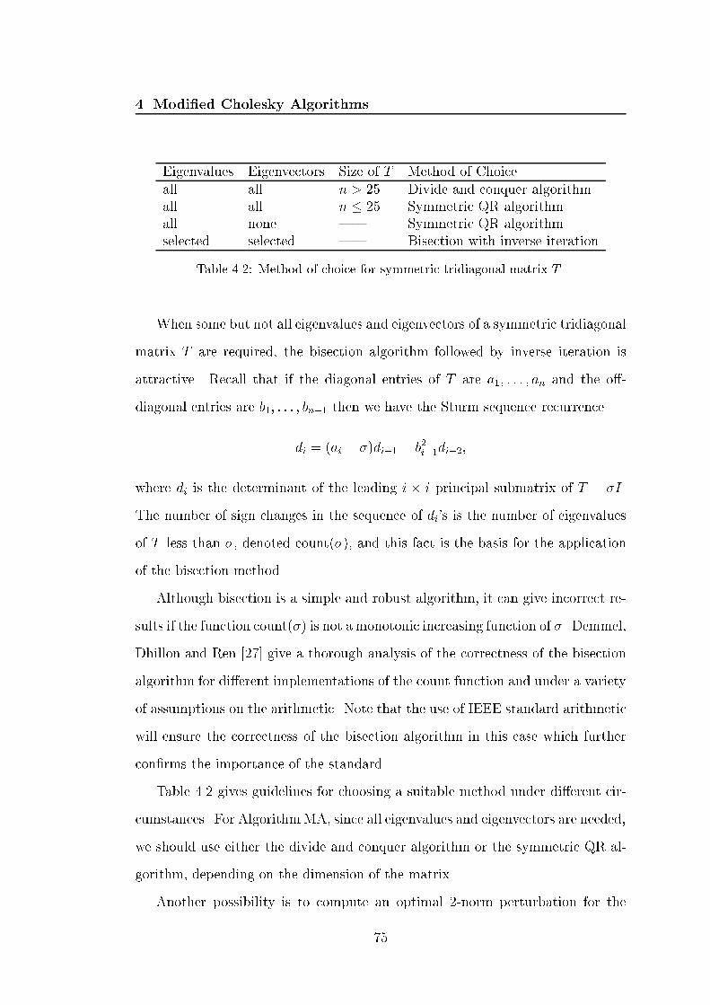
4. Modi�ed Cholesky AlgorithmsEigenvalues Eigenvectors Size of T Method of Choiceall all n > 25 Divide and conquer algorithmall all n � 25 Symmetric QR algorithmall none | Symmetric QR algorithmselected selected | Bisection with inverse iterationTable 4.2: Method of choice for symmetric tridiagonal matrix T .When some but not all eigenvalues and eigenvectors of a symmetric tridiagonalmatrix T are required, the bisection algorithm followed by inverse iteration isattractive. Recall that if the diagonal entries of T are a1; : : : ; an and the o�-diagonal entries are b1; : : : ; bn�1 then we have the Sturm sequence recurrencedi = (ai � �)di�1 � b2i�1di�2;where di is the determinant of the leading i � i principal submatrix of T � �I.The number of sign changes in the sequence of di's is the number of eigenvaluesof T less than �, denoted count(�), and this fact is the basis for the applicationof the bisection method.Although bisection is a simple and robust algorithm, it can give incorrect re-sults if the function count(�) is not a monotonic increasing function of �. Demmel,Dhillon and Ren [27] give a thorough analysis of the correctness of the bisectionalgorithm for di�erent implementations of the count function and under a varietyof assumptions on the arithmetic. Note that the use of IEEE standard arithmeticwill ensure the correctness of the bisection algorithm in this case which furthercon�rms the importance of the standard.Table 4.2 gives guidelines for choosing a suitable method under di�erent cir-cumstances. For AlgorithmMA, since all eigenvalues and eigenvectors are needed,we should use either the divide and conquer algorithm or the symmetric QR al-gorithm, depending on the dimension of the matrix.Another possibility is to compute an optimal 2-norm perturbation for the75

4. Modi�ed Cholesky Algorithmssymmetric tridiagonal matrix, for which only its minimum eigenvalue is required.That is, in the notation of Algorithm MA, T := eT + �min(eT )I. In this case, thebisection method is the method of choice.4.6 Comparison of AlgorithmsHere we compare the GMW and SE algorithms, Algorithm MC and AlgorithmMA according to their theoretical aspects.The bounds (4.10) and (4.16) can be compared with (4.22) for Algorithm MCand Algorithm MA. The bound (4.22) has the advantage of directly comparingthe perturbation made by Algorithm MC and Algorithm MA with the optimalone, de�ned as in (4.17) and evaluated in Theorem 4.4.1, and it is potentially amuch smaller bound than (4.10) and (4.16) if j�min(A)j � j�max(A)j and �2(LLT )is not too large.All four algorithms satisfy objective (O1) of not modifying a su�ciently pos-itive de�nite matrix, though for the GMW and SE algorithms no condition anal-ogous to (4.20) that quanti�es \su�ciently" in terms of �min(A) is available.Bounds for �2(A + E) that are exponential in n hold for the GMW and SEalgorithms [78]. The same is true for Algorithm MC and MA; see (4.23){(4.27).To summarize, in terms of the objectives of Section 4.1 for a modi�ed Choleskyalgorithm, Algorithm MC and Algorithm MA are theoretically competitive withthe GMW and SE algorithms, with the weakness that if �2(LLT ) is large thenthe bound on kEk2 is weak.When applied to an inde�nite matrix, the GMW and SE algorithms provideinformation that enables a direction of negative curvature of the matrix to beproduced; these directions are required in certain algorithms for unconstrainedoptimization in order to move away from non-minimizing stationary points. Foran inde�nite matrix, Algorithm MC provides immediate access to a direction of76

4. Modi�ed Cholesky Algorithmsnegative curvature from the LDLT factorization computed in step 1 of AlgorithmMC. Because �(L) is bounded, this direction satis�es conditions required for con-vergence theory [67]. For Algorithm MA, we can use the bisection with inverseiteration to compute the most negative eigenvalue and its corresponding eigen-vector of the symmetric tridiagonal matrix to gain information about a directionof negative curvature.Finally, we consider the behaviour of the algorithms in the presence of round-ing error. Algorithm MC is backward stable because the underlying factorizationis [58]: barring large element growth in block LDLT factorization with the BBKpivoting strategy, the algorithm produces LDLT factors not of P (A+E)P T , butof P (A + E + F )P T , where kFk2 � cnukA + Ek2 with cn a constant. We candeduce the stability of Algorithm MA using the same reasoning. Although nocomments on numerical stability are given in [37] and [78], a simple argumentshows that the GMW and SE algorithms are backward stable. Apply either algo-rithm to A, obtaining the Cholesky factorization P (A+E)P T = RTR. Now applythe same algorithm to P (A + E)P T : it will not need to modify P (A + E)P T ,so it will return the same computed R factor. But since no modi�cation wasrequired, the algorithm must have carried out a standard Cholesky factorization.Since Cholesky factorization is a backward stable process, the modi�ed Choleskyalgorithm must itself be backward stable.4.7 Numerical ExperimentsWe have experimented with Matlab implementations of Algorithm MC, Algo-rithm MA, and the GMW and SE algorithms. The M-�le for the GMW algorithmwas provided by Margaret Wright and sets the tolerance � = 2umaxf� + �; 1g,where 2u is the value of Matlab's variable eps. The M-�le for the SE algo-rithm was provided by Elizabeth Eskow and sets the tolerance � = (2u)1=3. In77

4. Modi�ed Cholesky AlgorithmsAlgorithm MC and Algorithm MA, we set � = pukAk1.The aims of the experiments are as follows: to see how well the Frobeniusnorm of the perturbation E produced by Algorithm MC and Algorithm MAapproximates the distance �F (A; �) de�ned in (4.17), and to compare the normsof the perturbations E and the condition numbers of A+E produced by the threealgorithms. We measure the perturbation E by the ratios F = kEkF�F (A; �) ; 2 = kEk2j�min(A)j ;which di�er only in their normalization and the choice of norm. Both AlgorithmMC and Algorithm MA attempt to make F close to 1. The quantity 2 is usedby Schnabel and Eskow [78] to compare the performance of the GMW and SEalgorithms; since E is diagonal for these algorithms, 2 compares the amountadded to the diagonal with the minimum diagonal perturbation that makes theperturbed matrix positive semide�nite.First, we note that the experiments of Schnabel and Eskow show that theSE algorithm can produce a substantially smaller value of 2 than the GMWalgorithm. Schnabel and Eskow also identi�ed a 4 � 4 matrix for which theGMW algorithm signi�cantly outperforms the SE algorithm:A = 2666666641890:3 �1705:6 �315:8 3000:31538:3 284:9 �2706:652:5 �501:24760:8

377777775 ; (4.29)with �(A) = f�0:39; �0:34; �0:25; 8:2� 103g. We give our results in Table4.3; they show that Algorithm MC and Algorithm MA can also signi�cantlyoutperform the SE algorithm.We ran a set of tests similar to those of Schnabel and Eskow [78]. The matricesA are of the formA = Q�QT , where � = diag(�i) with the eigenvalues �i from one78

4. Modi�ed Cholesky AlgorithmsMC MA GMW SE F 1:3 1:1 2:7 3:7� 103 2 1:7 1:1 2:7 2:8� 103Table 4.3: Measures of E for the 4� 4 matrix (4.29).n: 25 50 100max 523 2188 8811mean 343:9 1432:8 5998:4Table 4.4: Number of comparisons for the BBK pivoting strategy.of three random uniform distributions: [�1; 104], [�1; 1] and [�104;�1]. For the�rst range, one eigenvalue is generated for the range [�1; 0) to ensure that A hasat least one negative eigenvalue. The matrix Q is a random orthogonal matrixfrom the Haar distribution, generated using the routine qmult from the TestMatrix Toolbox [54], which implements an algorithm of Stewart [83]. For eacheigenvalue distribution we generated 30 di�erent matrices, each corresponding toa fresh example of � and of Q. We took n = 25; 50; 100. The ratios F and 2 areplotted in Figures 4.1{4.3. Figures 4.4{4.6 plot the condition numbers �2(A+E)for n = 25; 50; 100; Table 4.4 reports the number of comparisons used by theBBK pivoting strategy on these matrices for each n; the maximum number ofcomparisons is less than n2 in each case.In Figure 4.7 we report results for three nonrandom matrices from the TestMatrix Toolbox. Clement is a tridiagonal matrix with eigenvalues plus and minusthe numbers n� 1, n� 3, n� 5; : : : ; (1 or 0). Dingdong is the symmetric n� nHankel matrix with (i; j) element 0:5=(n� i� j +1:5), whose eigenvalues clusteraround �=2 and ��=2. Ipjfact is the Hankel matrix with (i; j) element 1=(i+j)!.Our conclusions from the experiments are as follows.79

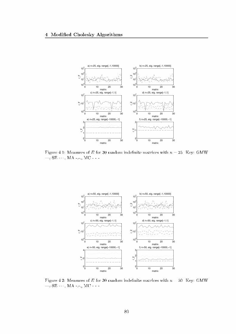
4. Modi�ed Cholesky Algorithms0 10 20 30

100

101

102

103

matrix

r_F

a) n=25, eig. range[−1,10000]

0 10 20 3010

0

101

102

matrix

r_F

c) n=25, eig. range[−1,1]

0 10 20 300

1

2

3

matrix

r_F

e) n=25, eig. range[−10000,−1]

0 10 20 3010

0

101

102

103

matrix

r_2

b) n=25, eig. range[−1,10000]

0 10 20 3010

0

101

102

matrix

r_2

d) n=25, eig. range[−1,1]

0 10 20 300

1

2

matrix

r_2

f) n=25, eig. range[−10000,−1]

Figure 4.1: Measures of E for 30 random inde�nite matrices with n = 25. Key: GMW|, SE � � � , MA -:-:, MC - - -.0 10 20 30

100

101

102

103

matrix

r_F

a) n=50, eig. range[−1,10000]

0 10 20 3010

0

101

102

matrix

r_F

c) n=50, eig. range[−1,1]

0 10 20 300

2

4

matrix

r_F

e) n=50, eig. range[−10000,−1]

0 10 20 3010

0

101

102

103

matrix

r_2

b) n=50, eig. range[−1,10000]

0 10 20 3010

0

101

102

matrix

r_2

d) n=50, eig. range[−1,1]

0 10 20 300

1

2

3

matrix

r_2

f) n=50, eig. range[−10000,−1]

Figure 4.2: Measures of E for 30 random inde�nite matrices with n = 50. Key: GMW|, SE � � � , MA -:-:, MC - - -.80

4. Modi�ed Cholesky Algorithms0 10 20 30

100

101

102

103

matrix

r_F

a) n=100, eig. range[−1,10000]

0 10 20 3010

0

101

102

103

matrix

r_F

c) n=100, eig. range[−1,1]

0 10 20 300

2

4

matrix

r_F

e) n=100, eig. range[−10000,−1]

0 10 20 3010

0

101

102

103

matrix

r_2

b) n=100, eig. range[−1,10000]

0 10 20 3010

0

101

102

103

matrix

r_2

d) n=100, eig. range[−1,1]

0 10 20 300

1

2

3

matrix

r_2

f) n=100, eig. range[−10000,−1]

Figure 4.3: Measures of E for 30 random inde�nite matrices with n = 100. Key: GMW|, SE � � � , MA -:-:, MC - - -.0 5 10 15 20 25 30

100

105

1010

matrix

kappa_2

a) n=25, eig. range[−1,10000]

0 5 10 15 20 25 3010

0

105

1010

matrix

kappa_2

b) n=25, eig. range[−1,1]

0 5 10 15 20 25 3010

0

101

102

103

matrix

kappa_2

c) n=25, eig. range[−10000,−1]

Figure 4.4: Condition numbers �2(A+E) for 30 random inde�nite matrices with n = 25.Key: GMW |, SE � � � , MA -:-:, MC - - -.81

4. Modi�ed Cholesky Algorithms0 5 10 15 20 25 30

100

105

1010

matrix

kappa_2

a) n=50, eig. range[−1,10000]

0 5 10 15 20 25 3010

0

105

1010

1015

matrix

kappa_2

b) n=50, eig. range[−1,1]

0 5 10 15 20 25 3010

0

102

104

matrix

kap

pa_2

c) n=50, eig. range[−10000,−1]

Figure 4.5: Condition numbers �2(A+E) for 30 random inde�nite matrices with n = 50.Key: GMW |, SE � � � , MA -:-:, MC - - -.0 5 10 15 20 25 30

100

105

1010

1015

matrix

kappa_2

a) n=100, eig. range[−1,10000]

0 5 10 15 20 25 3010

0

105

1010

1015

matrix

ka

ppa_2

b) n=100, eig. range[−1,1]

0 5 10 15 20 25 3010

0

105

matrix

kappa_2

c) n=100, eig. range[−10000,−1]

Figure 4.6: Condition numbers �2(A + E) for 30 random inde�nite matrices withn = 100. Key: GMW |, SE � � � , MA -:-:, MC - - -.82

4. Modi�ed Cholesky Algorithms20 40 60 80 100

100

101

n

r_F

a) clement(n,1)

20 40 60 80 100

100

101

n

r_2

b) clement(n,1)

20 40 60 80 10010

0

102

n

r_F

c) dingdong(n)

20 40 60 80 10010

0

102

n

r_2

d) dingdong(n)

20 40 60 80 10010

−1

100

101

n

r_F

e) ipjfact(n,1)

20 40 60 80 10010

−1

100

101

n

r_2

f) ipjfact(n,1)

Figure 4.7: Measures for three nonrandom matrices. Key: GMW |, SE � � � , MA -:-:,MC - - -.1. None of the four algorithms is uniformly better that the others in terms ofproducing a small perturbation E, whichever measure F or 2 is used. Allfour algorithms can produce values of F and 2 signi�cantly greater than1, depending on the problem.2. Algorithm MC produced F of order 103 for the eigenvalue distribution[�1; 104] for each n, and the values of �2(LLT ) were approximately 100 F ineach such case. However, often F was of order 1 when �2(LLT ) was of order102 or 103, so a large value of �2(LLT ) is only a necessary condition, not asu�cient one, for poor performance of Algorithm MC; in other words, thebounds of Section 4.4 can be weak. Similar observations hold for AlgorithmMA.3. The condition numbers �2(A+E) vary greatly among the algorithms. Ourexperience is that for � = pukAk1 Algorithm MC fairly consistently pro-duces conditions of order 100=pu; the condition number is, as predicted by83

4. Modi�ed Cholesky Algorithms(4.23), much smaller for the random matrices with eigenvalues on the range[�104;�1], because the algorithm attempts to perturb all the eigenvaluesto � and (4.23) is reduced to �2(A + E) � �2(LLT ). Again, similar con-clusions hold for Algorithm MA. The condition numbers produced by theGMW and SE algorithms vary greatly with the type of matrix.The fact that F is close to 1 for the random matrices with eigenvalues in therange [�104;�1] for Algorithm MC and Algorithm MA is easily explained. LetA be negative de�nite. Then Algorithm MC computes P (A+E)P T = L(�I)LT .Hence F = kEkF(P�i��(�i � �)2)1=2� kEkFkAkF = kA� � � P TLLTPkFkAkF� kAkF + �kLLTkFkAkF� 1 + (4n2 � 3n)�kAkF ;using (4.24). Meanwhile, Algorithm MA computes P (A+E)P T = LQ(�I)QTLT ,where QQT = I. We have F = kEkF(P�i��(�i � �)2)1=2� kEkFkAkF = kA� � � P TLQQTLTPkFkAkF� kAkF + �kLLTkFkAkF� 1 + (n2 � n+ 2)�2kAkF ;using (4.26). So F can exceed 1 only by a tiny amount for Algorithm MC andAlgorithm MA applied to a negative de�nite matrix, irrespective of �2(LLT ). Itis an open question to explain why F are approximately 2 and 4 for the GMWand SE algorithms respectively for this class of matrices.84

4. Modi�ed Cholesky Algorithms4.8 Concluding RemarksAlgorithm MC, based on a block LDLT factorization with the bounded Bunch{Kaufman pivoting strategy, and Algorithm MA, based on Aasen's LTLT factor-ization with partial pivoting, merit consideration as alternatives to the algorithmsof Gill, Murray and Wright, and Schnabel and Eskow. The results in Section 4.7suggest that the new algorithms are competitive with the GMW and SE algo-rithms in terms of the objectives (O1){(O4) listed in Section 4.1. Algorithms MCand MA have the advantages that the extent to which they satisfy the objectivesis neatly, although not sharply, described by the bounds of Sections 4.4 and 4.5.Algorithms MC and MA can be implemented by augmenting existing softwarewith just a small amount of additional code. In particular, for Algorithm MC, wecan use the e�cient implementations for both dense and sparse matrices writtenby Ashcraft, Grimes and Lewis [6], which make extensive use of level 2 and3 BLAS for e�ciency on high-performance machines. For Algorithm MA, theLTLT factorization is implemented in IMSL Fortran 90 MP Library [48], [90].Since all four algorithms can \fail", that is, they can produce unacceptablylarge perturbations, it is natural to ask how failure can be detected and whatshould be done about it. The GMW and SE algorithms produce their (diag-onal) perturbations explicitly, so it is trivial to evaluate their norms. For Al-gorithm MC and Algorithm MA, the perturbations to A have the form E =P TL(D + F )LTP � A, which would require O(n3) operations to form explicitly.However, we can estimate kEk1 using the norm estimator from [52] (which is im-plemented in LAPACK). The estimator require the formation of products Ex forcertain vectors x, and these can be computed in O(n2) operations; the estimateproduced is a lower bound that is nearly always within a factor of 3 of the truenorm. For all four algorithms, then, we can inexpensively test whether the per-turbation produced is acceptably small. Unfortunately, for none of the algorithms85

4. Modi�ed Cholesky Algorithmsis there an obvious way to improve a modi�ed factorization that makes too biga perturbation; whether improvement is possible, preferably cheaply, is an openquestion. Of course one can always resort to computing an optimal perturbationby computing the eigensystem of A and using the formulae in Theorem 4.4.1.We note that we have approached the problem of modi�ed Cholesky factor-ization from a purely linear algebra perspective. An important test of a modi�edCholesky algorithm is to evaluate it in an optimization code on representativeproblems, as was done by Schlick [77] for the GMW and SE algorithms. Suchtesting is beyond the scope of this thesis but would produce valuable informationabout the practical performance of the di�erent algorithms.

86

Chapter 5Modifying the Inertia of MatricesArising in Optimization5.1 IntroductionA block 2� 2 partitioning C = 24H AAT �M35of a symmetric matrix C arises in a number of applications, including constrainedoptimization, least squares problems and Navier{Stokes problems, as explainedin the next section. The matrix M is positive semide�nite, but H can be in-de�nite, depending on the application. In constrained optimization, a \secondorder su�ciency" condition leads to the problem of perturbing H so that C has aparticular inertia. It is this problem that motivated our work. We can view thischapter as an attempt to extend the notion of modi�ed Cholesky factorization toconstrained optimization.We present some background material on congruence transformations in Sec-tion 5.3, including an extension of Ostrowski's theorem (Theorem 4.4.2) to trans-formations with a rectangular matrix. In Section 5.4 we derive some useful inertiaproperties of the matrix C. How to make a minimal norm (full) perturbation toincrease the number of nonnegative eigenvalues of a symmetric matrix by a givenamount is shown in Section 5.5. The main result of this chapter is in Section5.6, in which we derive, for any unitarily invariant norm, a perturbation of H(only) of minimal norm that increases the number of nonnegative eigenvalues ofC by a given amount. For optimization applications, another way of writing the87

5. Modifying the Inertia of Matrices Arising in Optimizationsecond order su�ciency condition is based on projecting H into the null space ofA. We use this approach in Section 5.7 to derive another expression for a minimalnorm perturbation to H that achieves the su�ciency condition. In Section 5.8 weconsider how to implement our results in the optimization application and showthat directions of negative curvature are produced as a by-product of the compu-tation. Numerical experiment results are reported in Section 5.9 and concludingremarks are given in Section 5.10.5.2 A Symmetric Block 2�2 Matrix and its Ap-plicationsAny symmetric matrix C can be written in the formC = 24 n mn H ATm A �M 35;where H 2 Rn�n and M 2 Rm�m are symmetric and A 2 Rn�m . The reasonfor using a block 2 � 2 partitioning and for placing a minus sign in front of the(2; 2) block is that C then conveniently represents some particular cases arisingin applications, which we now describe in roughly decreasing order of generality.1. When M is diagonal and positive de�nite, C is the \primal-dual" matrixarising in certain interior methods for the general nonlinear programmingproblem [32], [33]. Here, H is the Hessian of the Lagrangian function andAT is the Jacobian of the constraint functions. The matrix C also arisesin penalty function methods for nonlinear programming, with M a positivemultiple of the identity matrix [43]. In these applications both m � n andm � n are possible. 88

5. Modifying the Inertia of Matrices Arising in Optimization2. When M = 0, C is the Karush{Kuhn{Tucker (KKT) matrix, which ariseswhen Newton's method or a quasi-Newton method is applied to the problemminx F (x) subject to ATx = b; (5.1)where F : Rn ! R and m � n, [20, p. 123], [34], [44]. To be precise,Newton's method leads to the equations24Hk AAT 03524pk�k35 = 24�gk0 35 ;where H is the Hessian of F or an approximation to it, g is the gradientof F , p is a search direction, and � is a Lagrange multiplier, and where asubscript k denotes evaluation at the kth iterate.3. For M = 0 and H = diag(Ip;�Iq) where p + q = n, C is the augmentedsystem matrix arising in the inde�nite least squares problemminx (b� Ax)TH(b� Ax);where m � n [16]. This problem reduces to the standard least squaresproblem when q = 0.4. If H and M are positive de�nite, then C matches precisely the de�nitionof a symmetric quaside�nite matrix [89]. Such matrices arise in interiormethods for linear and quadratic programming and much is known aboutthe existence and stability of their LDLT factorizations [38], [89].5. Matrices with H positive de�nite and M = 0 arise in discretized incom-pressible Navier{Stokes equations [79], and their spectral properties areimportant in the development of preconditioned iterative methods [30].6. The matrix with H = �I and M = �I (� > 0) appears in the augmentedsystem corresponding to the damped least squares problemminx kb� Axk22 + �2kxk22;89

5. Modifying the Inertia of Matrices Arising in Optimizationsee Saunders [76].7. For H positive de�nite and M = 0, C is the augmented system matrixarising in the generalized least squares problem minx(b�Ax)TH�1(b�Ax)(m � n) [8, Section 4.3.2]; H = I gives the standard least squares problem.In quasi-Newton methods for the linear-equality constrained problem (5.1) it isdesirable that the Hessian approximationH satisfy the \second order su�ciency"condition [44] pTHp > 0 for all nonzero p such that ATp = 0: (5.2)One equivalent condition is that the projected Hessian ZTHZ be positive de�nite,where the columns of Z form a basis for the null space null(AT ). Less obviously,the condition (5.2) is also equivalent to requiring the so-called KKT matrixK = 264 n mn H ATm A 0 375; (5.3)to have a certain inertia, as shown by Gould [42]. Recall that the inertia ofa symmetric matrix is an ordered triple (i+; i�; i0), where i+ is the number ofpositive eigenvalues, i� is the number of negative eigenvalues, and i0 is the numberof zero eigenvalues. We writeinertia(A) = (i+(A); i�(A); i0(A)):Theorem 5.2.1 (Gould) Let A be of full rank m. The condition (5:2) holds ifand only if K has the inertia (n;m; 0).Proof: Let A have the QR factorizationA = Q24R035 = hY Zi24R035 ;90

5. Modifying the Inertia of Matrices Arising in Optimizationwhere Y 2 Rn�m , Z 2 Rn�(n�m) and R 2 Rm�m . ThenK = 266664 H Q24R035hRT 0iQT 0377775 = 24Q 00 I35266664 QTHQ 24R035hRT 0i 0

37777524Q 00 I35T� 26664Y THY Y THZ RZTHY ZTHZ 0RT 0 037775 = : eK;where � denotes congruence (in fact, this �rst transformation is an orthogonalsimilarity which preserves the symmetry and the eigenvalues). Now de�ne thenonsingular matrix W = 26664Im 0 �12Y THYR�T0 In�m �ZTHYR�T0 0 R�T 37775 :It is straightforward to verify thatW eKW T = 26664 0 0 Im0 ZTHZ 0Im 0 0 37775 :By constructing eigenvectors [ei 0 ei]T and [ei 0 � ei]T where ei is the ith rowof the identity matrix Im, it is easily seen that the eigenvalues of W eKW T are 1and �1, each repeated m times, together with the n�m eigenvalues of ZTHZ.Since Z spans the null space of AT , ZTHZ is positive de�nite if and only if (5.2)holds, which completes the proof. 2The requirement (5.2) and Theorem 5.2.1 the problem give rise to the problemof perturbingH so thatK achieves the desired inertia (n;m; 0) [42]. The matrixAmust not be perturbed because this would correspond to changing the constraintsin (5.1). The same problem is relevant for the primal-dualmatrix withM diagonal91

5. Modifying the Inertia of Matrices Arising in Optimizationand positive semide�nite [32]. We �nd a minimal-norm solution to a more generalversion of this inertia perturbation problem in Section 5.6. In Section 5.7 weconsider an alternative approach to perturbing H to satisfy (5.2), based on theprojected Hessian. First, we develop some necessary background theory.5.3 Rectangular Congruence TransformationsSylvester's inertia theorem says that the inertia of a symmetric matrix is preservedunder a congruence transformation. Ostrowski's theorem (Theorem 4.4.2) [60,Thm. 4.5.9], [69], [92] goes further by explaining by how much the magnitudesof the eigenvalues can change. In the following statement of Ostrowski's theorem[60, Cor. 4.5.11] the transforming matrix X is permitted to be singular, in whichcase the transformation matrix XTAX is not a congruence transformation andcan change the inertia. Throughout this chapter the eigenvalues of a symmetricn � n matrix are ordered �1 � � � � � �n, and �i(A) denotes the ith smallesteigenvalue of A.Theorem 5.3.1 (Ostrowski) Let A 2 Rn�n be symmetric and X 2 Rn�n .Then for each k, k = 1:n, �k(XTAX) = �k�k(A)where �1(XTX) � �k � �n(XTX). 2We now generalize Ostrowski's theorem to \rectangular congruences", in whichthe transformating matrix X is nonsquare. Such transformations change the di-mension and hence the inertia, but for full rank X the amount by which inertiacan change depends on the di�erence of the dimensions of X, as shown in thecorollaries below. First, we consider matrices X with at least as many rows ascolumns. 92

5. Modifying the Inertia of Matrices Arising in OptimizationTheorem 5.3.2 Let A 2 Rn�n be symmetric and let X 2 Rn�m (n � m). Then�k(XTAX) = �k�k; k = 1:m;where �k(A) � �k � �k+n�m(A); k = 1:m;and �1(XTX) � �k � �m(XTX).Proof: Let X = U 24�035V Tbe a singular value decomposition, where U 2 Rn�n and V 2 Rm�m are orthogonaland � 2 Rm�m is diagonal. ThenXTAX = V [�T 0]UTAU 24�035V T = V (�T eA11�)V T ;where eA11 is the leading principal submatrix of order m of eA = UTAU . ByOstrowski's theorem,�k(XTAX) = �k(�T eA11�) = �k( eA11)�k;where �1(XTX) = �1(�T�) � �k � �m(�T�) = �m(XTX):Cauchy's interlace theorem [71, p. 186] shows that�k(A) = �k( eA) � �k( eA11) � �k+n�m( eA) = �k+n�m(A); k = 1:m;which yields the result. 2In the case where X has orthonormal columns (so that �k � 1), Theorem5.3.2 reduces to the Poincar�e separation theorem [60, Cor. 4.3.16], [84, Cor. 4.4,p. 198]. 93

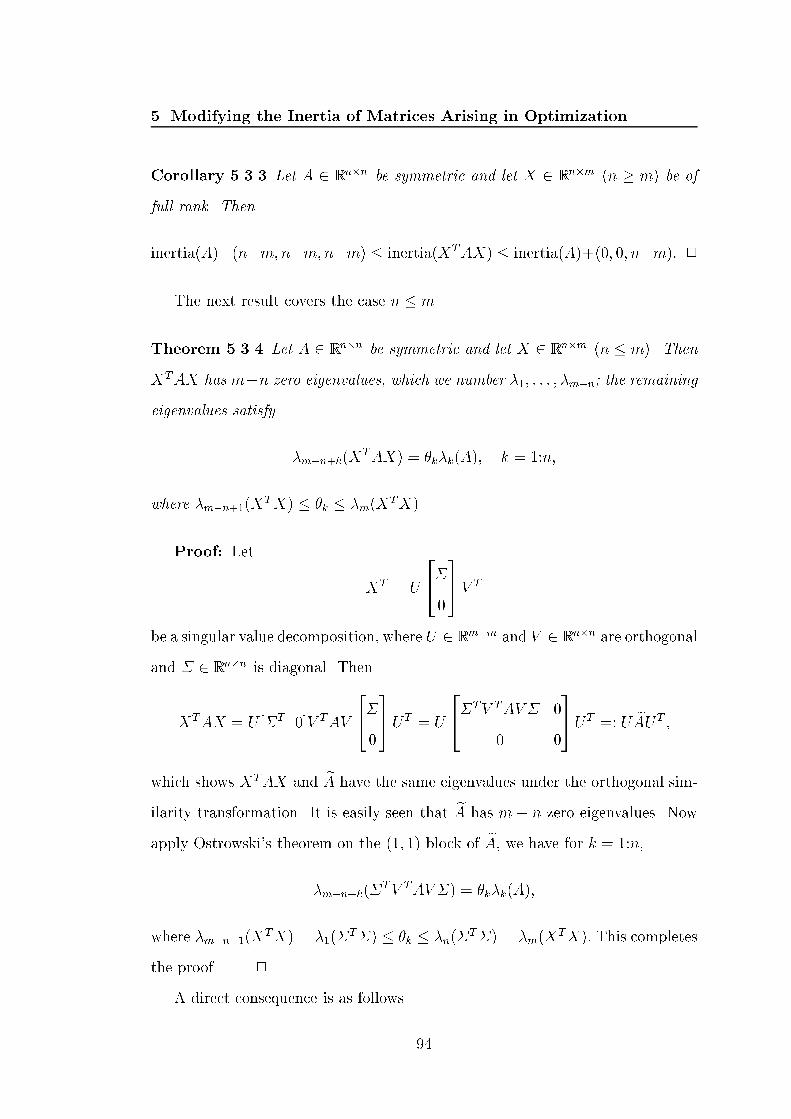
5. Modifying the Inertia of Matrices Arising in OptimizationCorollary 5.3.3 Let A 2 Rn�n be symmetric and let X 2 Rn�m (n � m) be offull rank. Theninertia(A)�(n�m;n�m;n�m) � inertia(XTAX) � inertia(A)+(0; 0; n�m): 2The next result covers the case n � m.Theorem 5.3.4 Let A 2 Rn�n be symmetric and let X 2 Rn�m (n � m). ThenXTAX has m�n zero eigenvalues, which we number �1; : : : ; �m�n; the remainingeigenvalues satisfy �m�n+k(XTAX) = �k�k(A); k = 1:n;where �m�n+1(XTX) � �k � �m(XTX).Proof: Let XT = U 24�035V Tbe a singular value decomposition, where U 2 Rm�m and V 2 Rn�n are orthogonaland � 2 Rn�n is diagonal. ThenXTAX = U [�T 0]V TAV 24�035UT = U 24�TV TAV� 00 035UT =: U eAUT ;which shows XTAX and eA have the same eigenvalues under the orthogonal sim-ilarity transformation. It is easily seen that eA has m � n zero eigenvalues. Nowapply Ostrowski's theorem on the (1; 1) block of eA, we have for k = 1:n,�m�n+k(�TV TAV�) = �k�k(A);where �m�n+1(XTX) = �1(�T�) � �k � �n(�T�) = �m(XTX): This completesthe proof. 2A direct consequence is as follows. 94

5. Modifying the Inertia of Matrices Arising in OptimizationCorollary 5.3.5 Let A 2 Rn�n be symmetric and let X 2 Rn�m (n � m) be offull rank. Then inertia(XTAX) = inertia(A) + (0; 0; m� n): 25.4 Inertia Properties of CIn this section we derive some inertia properties of the matrixC = 264 n mn H ATm A �M 375: (5.4)Assume that H is nonsingular. We have24 I 0�ATH�1 I3524H AAT �M35 = 24H A0 �M � ATH�1A35= 24H 00 �M � ATH�1A3524I H�1A0 I 35 ;which shows that C � 24H 00 �M � ATH�1A35 : (5.5)This congruence is the basis of the following lemmas, the �rst of which is containedin [49, Thm. 3].Lemma 5.4.1 If H is nonsingular,M = 0 and A has full rank then inertia(C) �(m;m; 0) if n � m and inertia(C) = (n; n;m� n) if n � m.Proof: Let inertia(H) = (a; b; 0) and inertia(�ATH�1A) = (p; q; r). Thenfrom (5.5) we have inertia(C) = (a+ p; b+ q; r):95

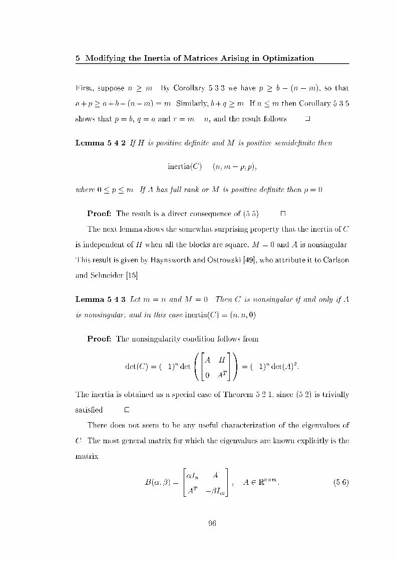
5. Modifying the Inertia of Matrices Arising in OptimizationFirst, suppose n � m. By Corollary 5.3.3 we have p � b � (n � m), so thata+ p � a+ b� (n�m) = m. Similarly, b+ q � m. If n � m then Corollary 5.3.5shows that p = b, q = a and r = m� n, and the result follows. 2Lemma 5.4.2 If H is positive de�nite and M is positive semide�nite theninertia(C) = (n;m� p; p);where 0 � p � m. If A has full rank or M is positive de�nite then p = 0.Proof: The result is a direct consequence of (5.5). 2The next lemma shows the somewhat surprising property that the inertia of Cis independent of H when all the blocks are square, M = 0 and A is nonsingular.This result is given by Haynsworth and Ostrowski [49], who attribute it to Carlsonand Schneider [15].Lemma 5.4.3 Let m = n and M = 0. Then C is nonsingular if and only if Ais nonsingular, and in this case inertia(C) = (n; n; 0).Proof: The nonsingularity condition follows fromdet(C) = (�1)n det0@24A H0 AT351A = (�1)n det(A)2:The inertia is obtained as a special case of Theorem 5.2.1, since (5.2) is triviallysatis�ed. 2There does not seem to be any useful characterization of the eigenvalues ofC. The most general matrix for which the eigenvalues are known explicitly is thematrix B(�; �) = 24�In AAT ��Im35 ; A 2 Rn�m : (5.6)96

5. Modifying the Inertia of Matrices Arising in OptimizationSaunders [76] shows that if A has rank p with nonzero singular values �i, i = 1:p,then �(B(�; �)) = 8>>><>>>: 12(�� �)� ��2i + 14(� + �)2�1=2 ; i = 1:p;�; n� p times;��; m� p times: (5.7)The conclusions of Lemmas 5.4.1{5.4.3 are readily veri�ed for this matrix.Finally, we give inequalities that bound the eigenvalues of C away from zero,which is of interest for investigating conditioning. This lemma is a restatementof the \separation theorem" of v. Kempen [88].Lemma 5.4.4 If H is positive de�nite and M is positive semide�nite or positivede�nite, then the eigenvalues �i of C satisfy�1 � � � � � �m � ��min(M) < �min(H) � �m+1 � � � � � �m+n; (5.8)Proof: Let � be an eigenvalue of C and x a corresponding eigenvector andwrite Cx = �x as 24H AAT �M3524yz35 = �24yz35 :Premultiplying the �rst equation of the pair by yT and the second by zT , andsubtracting, yields yTHy � �yTy = �zTMz � �zT z;or yT (H � �I)y + zT (M + �I)z = 0: (5.9)If ��min(M) < � < �min(H) then H � �I and M + �I are positive de�nite and(5.9) yields a contradiction since y and z are not both zero. The inequalities (5.8)now follow from Lemma 5.4.2. 2 97

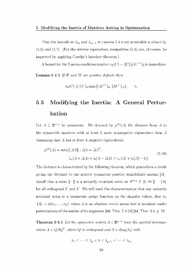
5. Modifying the Inertia of Matrices Arising in OptimizationThat the bounds on �m and �m+1 in Lemma 5.4.4 are attainable is shown by(5.6) and (5.7). (For the interior eigenvalues, inequalities (5.8) can, of course, beimproved by applying Cauchy's interlace theorem.)A bound for the 2-norm condition number �2(C) = kCk2kC�1k2 is immediate.Lemma 5.4.5 If H and M are positive de�nite then�2(C) � kCk2maxfkH�1k2; kM�1k2g: 25.5 Modifying the Inertia: A General Pertur-bationLet A 2 Rn�n be symmetric. We denoted by �(k)(A) the distance from A tothe symmetric matrices with at least k more nonnegative eigenvalues than A(assuming that A has at least k negative eigenvalues):�(k)(A) = minfk�Ak : �A = �AT ;i+(A+�A) + i0(A+�A) � i+(A) + i0(A) + kg: (5.10)The distance is characterized by the following theorem, which generalizes a resultgiving the distance to the nearest symmetric positive semide�nite matrix [51].Recall that a norm k � k is a unitarily invariant norm on Rn�n if kUAV k = kAkfor all orthogonal U and V . We will need the characterization that any unitarilyinvariant norm is a symmetric gauge function on the singular values, that is,kAk = �(�1; : : : ; �n), where � is an absolute vector norm that is invariant underpermutations of the entries of its argument [60, Thm. 7.4.24],[84, Thm. 3.6, p. 78].Theorem 5.5.1 Let the symmetric matrix A 2 Rn�n have the spectral decompo-sition A = Q�QT , where Q is orthogonal and � = diag(�i) with�1 � � � � � �p < 0 � �p+1 � � � � � �n;98

5. Modifying the Inertia of Matrices Arising in Optimizationand assume that p � k. Then for any unitarily invariant norm, an optimalperturbation in (5:10) is�A = Q diag(�i)QT ; �i = 8<: ��i; i = p� k + 1:p;0; otherwise: (5.11)and �(k)(A) = �(�1; : : : ; �n):Proof: A generalization of the Wielandt{Ho�man theorem [60, Thm. 7.4.51],[84, p. 205] says that if A and A+�A are symmetric thenk�Ak � k diag(�i(A+�A)� �i(A))kfor any unitarily invariant norm. If �A is a feasible perturbation in (5.10) thenk�Ak � k diag(0; : : : ; 0; �p�k+1(A+�A)� �p�k+1(A); : : : ;�p(A+�A)� �p(A); 0; : : : ; 0)k� k diag(0; : : : ; 0;��p�k+1(A); : : : ;��p(A); 0; : : : ; 0)k;where we have used �p(A + �A) � � � � � �p�k+1(A + �A) � 0 and the gaugefunction property of the norms. It is easily seen that equality is attained for theperturbation given in the statement of the theorem and that this perturbation isfeasible. 25.6 Modifying the Inertia: A Structured Per-turbationReturning to the partitioned matrix (5.4), we are interested in �nding a pertur-bation �H such that C +�C = 24H +�H AAT �M3599

5. Modifying the Inertia of Matrices Arising in Optimizationhas a given inertia. For the analysis in this section, C can be regarded as a generalblock 2�2 symmetric matrix|we will not need A to have full rank or the diagonalblocks to process any de�niteness properties, and m and n are arbitrary.For the KKT matrix, practical interest is in increasing the number of positiveeigenvalues (in view of Theorem 5.2.1 and Lemma 5.4.1), so we de�ne, analogouslyto (5.10), (k)(C) = minfk�Hk : �H = �HT ;i+(C +�C) + i0(C +�C) � i+(C) + i0(C) + kg: (5.12)Clearly, an optimal �H in (5.12) can be taken to be positive semide�nite and ofrank k, hence of the form �H = V V T with V 2 Rn�k (k � n). Our solution tothis problem is based on the following lemma. The lemma is not new; essentiallythe same result can be found in [4, Lem. 2.1] and [5, Cor. 2.2], for example.Lemma 5.6.1 Let A 2 Rn�n be symmetric and nonsingular and let W 2 Rn�k .Then i+(A +WW T ) + i0(A +WW T ) = i+(A) + i0(A) + k if and only if �Ik �W TA�1W is positive semide�nite.Proof: We have the congruencesB = 24 n kn A Wk W T �Ik 35 � 24A 00 �Ik �W TA�1W 35and, for a suitable permutation �,�TB� = 24�Ik W TW A 35 � 24�Ik 00 A +WW T35 :It follows thatinertia(A) + inertia(�Ik �W TA�1W ) = inertia(�Ik) + inertia(A+WW T );100

5. Modifying the Inertia of Matrices Arising in Optimizationthat is,inertia(A+WW T ) = inertia(A) + inertia(�Ik �W TA�1W )� inertia(�Ik):The result is immediate. 2We apply Lemma 5.6.1 with A the matrix C (assumed to be nonsingular) andW = 24 kn Vm 0 35:The lemma tells us that we need to minimize kV V Tk subject tohV T 0TiC�1 24V035 2 Rk�k (5.13)having all its eigenvalues less than or equal to �1. Writing G = C�1(1:n; 1:n),this constraint is �i(V TGV ) � �1; i = 1:k: (5.14)By Corollary 5.3.3, a matrix satisfying (5.14) exists only if G has at least knegative eigenvalues, which we assume to be the case. The following lemma andcorollary show how to minimize kV V Tk for any unitarily invariant norm subjectto (5.14).Lemma 5.6.2 Let A 2 Rn�n be symmetric with the spectral decomposition A =Q diag(�i)QT , where Q is orthogonal and�1 � � � � � �p�1 � 0 < �p � � � � � �n:Let X 2 Rn�k with k � n and assume that p � n � k + 1. All matrices X thatminimize all the singular values of X subject to satisfying the inequalities�i(XTAX) � 1; i = 1:k; (5.15)101

5. Modifying the Inertia of Matrices Arising in Optimizationare given by X = Q(1:n; n� k + 1:n) diag(�n�k+1; : : : ; �n)�1=2V; (5.16)where V 2 Rk�k is an arbitrary orthogonal matrix.Proof: LetX = U�V T ; � = 24S035 ; S = diag(�i) 2 Rk�kbe the singular value decomposition of X. ThenXTAX � I = V �TUTAU�V T � I = V (SBS � I)V T ;where B = (UTAU)(1:k; 1:k). The constraint (5.15) is therefore equivalent toSBS � I being positive semide�nite, which implies thatbii � 1�2i ; i = 1:k: (5.17)We wish to maximize the reciprocals ��2i . Now the diagonal of the symmetricmatrix B is largest in modulus when it contains the eigenvalues of B, that is,when B is diagonal, (5.17) is equivalent to (5.15). This fact is easily shown. LetM 2 Rn�n be symmetric. Then, for the Frobenius norm, we havekMk2F =Xi6=j m2ij +Xi m2ii �Xi m2ii:Equality holds in the inequality, and hence Pim2ii is maximized, when mij = 0for i 6= j. Therefore m11; : : : ; mnn must be the eigenvalues of M .Hence for optimality we need to choose U = Q(1:n; n � k + 1:n) and then,to attain the bounds in (5.17), �i = ��1=2n�k+i (note that the �i are arranged indecreasing order). The matrix V is arbitrary. 2Corollary 5.6.3 Under the condition of Lemma 5:6:2, the matrix (5:16) mini-mizes kXXTk subject to (5:15) for any unitarily invariant norm.102

5. Modifying the Inertia of Matrices Arising in OptimizationProof: The singular values of XXT are the squares of the singular values ofX, which are minimized by the matrix (5.16). The result follows from the gaugefunction property of unitarily invariant norms. 2We now summarize our �ndings in a theorem.Theorem 5.6.4 Let H 2 Rn�n and M 2 Rm�m be symmetric and A 2 Rn�m ,and let C = 24H AAT �M35 :Assume C is nonsingular and let G = C�1(1:n; 1:n). There exists a feasible per-turbation in the de�nition of (k)(C) if and only if G has at least k negativeeigenvalues. Let G = Q diag( i)QT be a spectral decomposition, where Q is or-thogonal and 1 � � � � � n. Then, for any unitarily invariant norm, an optimalperturbation in (5:12) is�H = �Q diag( �11 ; : : : ; �1k ; 0; : : : ; 0)QT (5.18)and, in terms of the underlying gauge function �, (k)(C) = �( �11 ; : : : ; �1k ; 0; : : : ; 0): 2 (5.19)The perturbation (5.18) is full, in general, so may not be a suitable pertur-bation when H is large and sparse. It is natural, therefore, to consider diagonalperturbations. The next result shows that a perturbation consisting of a suitablemultiple of the identity matrix is also optimal in the 2-norm. This result can bededuced from Theorem 5.6.4, but we give an independent proof for completeness.Theorem 5.6.5 Under the same condition as in Theorem 5:6:4, an optimal per-turbation in (5:12) in the 2-norm is�H = � �1k I: (5.20)103

5. Modifying the Inertia of Matrices Arising in OptimizationProof: Consider perturbations to C of the form �C = WW T withW = 264 nn �Im 0 375: (5.21)It is straightforward to prove an analogue of Lemma 5.6.1 which says that ifA 2 Rn�n is symmetric and nonsingular, W 2 Rn�k and p � k, then i+(A +WW T ) + i0(A+WW T ) = i+(A) + i0(A) + p if and only if �Ik �W TA�1W hasexactly p nonnegative eigenvalues. Applying this result to (5.21) we �nd that�H = WW T is a feasible perturbation in (5.12) if and only if �In � �2G has knonnegative eigenvalues, where G = C�1(1:n; 1:n). We are assuming that G hasat least k nonnegative eigenvalues, so the minimal value of �2 is �1= k. Thisgives k�Ck2 = �1= k, which, in view of (5.19), shows that (5.21) is an optimalperturbation in the 2-norm. 2Note that whereas the perturbation (5.18) increases i+ + i0 by exactly k, theperturbation (5.20) will increase it by more than k if k = k+1 = � � � = k+r withr � 1.5.7 A Projected Hessian ApproachFor the matrix C with n � m, there is an alternative way to �nd a perturbationto H of minimal norm such that the second order su�ciency condition (5.2)is satis�ed. As noted earlier, the condition (5.2) is equivalent to the projectedHessian ZTHZ being positive de�nite, where the columns of Z 2 Rn�(n�m) forma basis for null(AT ), which we will take to be orthonormal. Therefore we areinterested in solving the problemminfk�Hk : ZT (H +�H)Z is positive semide�niteg: (5.22)104

5. Modifying the Inertia of Matrices Arising in OptimizationFrom Theorem 5.5.1 we know that an optimal arbitrary perturbation E thatmakes ZTHZ + E positive semide�nite is, for any unitarily invariant norm,E = U diag(max(��i; 0))UT ; (5.23)where ZTHZ = U diag(�i)UT with �1 � � � � � �n�m is a spectral decomposition.Hence any feasible �H in (5.22) satis�eskEk � kZT�HZk � kZTk2k�HkkZk2 � k�Hk;using an inequality for unitarily invariant norms from [61, p. 211]. But theperturbation (5.23) is achieved in (5.22) by setting �H = ZEZT , and k�Hk �kZk2kEkkZTk2 � kEk. We conclude that�H = ZU diag(max(��i; 0))UTZT (5.24)is a solution to (5.22) for any unitarily invariant norm. For the 2-norm, anothersolution is �H = max(��1; 0)ZZT : (5.25)For the special case of the KKT matrix de�ned as in (5.3), for which (5.2) isequivalent to inertia(K) = (n;m; 0) by Theorem 5.2.1, the perturbation (5.24)is, necessarily, of the same norm as (5.18) for k = n � i+(K) in Theorem 5.6.4,although this equivalence is not obvious from the formulae.When M is positive de�nite, or M is positive semide�nite and A has fullrank, Lemma 5.4.2 shows that we can achieve the desired inertia (n;m; 0) bychoosing �H to make H+�H positive de�nite. Theorem 5.5.1 with k = p showsthat the smallest value of k�Hk2 for which H + �H is positive semide�nite ismax(��min(H); 0). By de�nition, this perturbation is at least as large as theoptimal ones (5.18) and (5.24), and from (5.24) we havek�Hk2 � max(��min(ZTHZ); 0);105

5. Modifying the Inertia of Matrices Arising in Optimizationwhich can be arbitrarily smaller than max(��min(H); 0). We note, in particular,that the perturbation (5.18), (5.20), (5.24) and (5.25) all have 2-norms uniformlybounded by kHk2, which is an important property for optimization application[44].We give a numerical example for illustration. Consider the KKT matrixK = 266664 �1 1 01 �100 10 1 0377775 ; �(K) = f�1:00� 102;�9:90� 10�1; 1:01� 10�2g;where the eigenvalues are given to three signi�cant �gures. Hence inertia(K) =(1; 2; 0), and we want to change the inertia to (2; 1; 0). SinceK�1 = 266664 �1 0 10 0 11 1 99

377775 ;we �nd immediately from Theorem 5.6.4 with k = 1 that�H = 241 00 035 (5.26)is a matrix of minimal norm, for any unitarily invariant norm, that changes theinertia of K to (1; 1; 1); indeedK +�K = 266640 1 01 �100 10 1 037775 ; �(K +�K) = f�1:00� 102; 0; 2:00� 10�2g:For the projected Hessian approach we have Z = [1 0]T , ZTHZ = �1 and (5.24)yields the perturbation (5.26). To achieve the inertia (2; 1; 0) that is required forthe condition (5.2) to hold, we can replace �H by (1 + �)�H for any � > 0.In order to perturb H to make it positive de�nite, which also produce thedesired inertia, which must make a perturbation of 2-norm at least ��min(H) =106

5. Modifying the Inertia of Matrices Arising in Optimization1:00� 102, which is two orders of magnitude larger than the minimal-norm per-turbation (5.26).5.8 Practical AlgorithmWe now turn to the optimization applications. We consider the situation wherea linear system Cx = b must be solved, but C needs to be perturbed in its (1; 1)block, if necessary, to ensure that it has the inertia (n;m; 0).We assume that a block LDLT factorization of C is computed,PCP T = LDLT ;where L is unit lower triangular and D is block diagonal with blocks of dimension1 or 2; P is a permutation matrix that can be chosen according to one of variouspivoting strategies mentioned in Chapter 2. Since C and D have the same inertiait is trivial to evaluate the inertia of C. If i+(C) is less than n then Theorem 5.6.4shows that to determine the optimal perturbation (5.18) we need to computethe k = n � i+(C) most negative eigenvalues of G = C�1(1:n; 1:n) and theircorresponding eigenvectors; for the optimal 2-norm perturbation (5.20) it su�cesto determine the kth most negative eigenvalue of G. To con�rm that there are knegative eigenvalue of G, we apply Cauchy's interlace theorem, which yields�i(G) � �i+m(C�1); i = 1:n:Hence if C has only i+(C) < n positive eigenvalues then G has at least n� i+(C)negative eigenvalues.Since C may be large and sparse it is undesirable to form G explicitly. There-fore we suggest that the k most negative eigenvalues of G and their correspondingeigenvectors be computed using the Lanczos algorithm, which requires only the107

5. Modifying the Inertia of Matrices Arising in Optimizationability to form matrix-vector products with G. To form y = Gx we note that24yz35 = C�1 24x035 ;where z 2 Rm is not of interest. Hence y is the �rst n components of the solutionto the linear system C 24yz35 = 24x035 ;which can be solved using the block LDLT factorization.Note that the perturbation (5.18) makes C +�C singular, since it perturbsk negative eigenvalues to the origin. Similarly, the perturbation (5.20) producesat least one zero eigenvalue. In practice a nonsingular C +�C is required, andthe natural approach is to modify the perturbations so that the eigenvalues aremoved to a positive tolerance � instead of 0.Having computed an optimal perturbation �H we have to refactorize C+�Cin order to solve (C +�C)x = b. It does not seem practical to apply updatingtechniques to the original factorization, since the update may not be of low rank.However, if M = 0, m � n and A 2 Rm�n has full column rank, we canupdate the KKT matrix K using a formula in Fletcher [31, ex. 12.12, p. 327], inwhich the pseudoinverse of A is required. GivenK +�K = 24H +�H AAT 035 ;we have (K +�K)�1 = K�1 � 240 00 S35 ; (5.27)where S = A+�H(A+)T and A+ = (ATA)�1AT is the pseudoinverse of A. Whensolving a linear system (K +�K)x = b using (5.27), the solution is given byx = K�1b� 240 00 S35 b:108

5. Modifying the Inertia of Matrices Arising in OptimizationNote that the block LDLT factorization ofK is readily available when determiningthe inertia of K. The constraint matrix AT , and hence the pseudoinverse A+,remains constant within an optimization application (at least for linear equalityconstrained optimizations), which means that A+ can be computed only oncevia a singular value decomposition or a QR factorization, so it may not be tooexpensive.In the case where M = 0, our algorithm provides, as a by product, a directionof negative curvature, which is de�ned as a vector p for which (cf. (5.2)) ATp = 0and pTHp < 0. Such directions are needed in nonlinear programming to achieveconvergence to points that satisfy second order necessary conditions for optimal-ity. Writing the perturbation (5.18) as �H = V V T , we know that the matrix(5.13), which we denote by S, is negative de�nite. NowS = hV T 0Ti24XY 35 ; where 24H AAT 03524XY 35 = 24V035 :Thus HX + AY = V and ATX = 0, which implies XTHX = ST = S. Thejth column xj of X satis�es xTj Hxj = sjj < 0, since S is negative de�nite, andATxj = 0. Thus, every column of X is a direction of negative curvature.An alternative approach is to work with the projected Hessian ZTHZ and tocompute an optimal perturbation �H from (5.24) or (5.25). Again, the Lanczosalgorithm can be used, this time to compute the negative eigenvalues of ZTHZ.5.9 Numerical ExperimentsNumerical experiments have been performed inMatlab where the unit roundo�u � 1:1� 10�16. We generated 50 random KKT matrices K with n = 20, m = 5and elements normally distributed with mean 0 and variance 1. The perturbationis taken to be (1+�)�H where the tolerance � = ukKk1, and the required inertiais (n;m; 0). 109

5. Modifying the Inertia of Matrices Arising in OptimizationFirst we focus on demonstrating that perturbations (5.18), (5.20), (5.24) and(5.25) can achieve the given inertia in practice. The inverse of K was formedexplicitly by Matlab function inv. Then the eigenvalues of G = K�1(1:n; 1:n)were computed using Matlab function eig. The null space Z was computed byMatlab function QR. In more than 90% of the test cases, all four perturbationsyielded the speci�c inertia. In a few cases that our perturbations gave the inertia(n+ 1; m� 1; 0), they were easily �xed by reducing the tolerance �.Then we implemented our practical algorithm in which G was not formedexplicitly and the eigenvalues were computed by the Lanczos method. An M-�lefor the Lanczos method was provided by Thierry Braconnier. Our conclusions ofthe experiments are as follows.1. When computing the optimal Frobenius norm perturbation (5.18), we needto compute the k most negative eigenvalues of G = K�1(1:n; 1:n), usingthe Lanczos method. This approach is of limited practical use because theLanczos method su�ers convergence di�culties when there are clusteredeigenvalues close to the origin. In our experiments, the Lanczos methodoften failed to converge, even if only two eigenvalues were needed. A shiftand invert technique was employed to overcome the problem. Essentially,it involves working with (G � b�I)�1 where b� is a good approximation tothe required eigenvalue �. Let x denote the eigenvector corresponding to�, and let � be an eigenvalue of (G� �I)�1. We haveGx = �x, (G� �I)x = (�� �)x, (G� �I)�1x = (�� �)�1x;which shows that G and (G� �I)�1 share the same set of eigenvectors, andtheir eigenvalues are related by � = (�� �)�1. Unfortunately, G then needsto be formed explicitly if the shift and invert technique is to be used.2. Finding the optimal 2-norm perturbation (5.20) gives the same problem as110

5. Modifying the Inertia of Matrices Arising in Optimizationabove. To determine the kth smallest eigenvalue, we have to compute allthe other k � 1 most negative eigenvalues. No existing eigenvalue solvercomputes a target eigenvalue which is not an extreme eigenvalue for a largeand possibly sparse matrix.3. When the projected Hessian approach is used, the Lanczos method canbe used to compute all the negative eigenvalues of ZTHZ to determine(5.24). We run into the same problem when clustered eigenvalues occur.For perturbation (5.25), we need the most negative eigenvalue of ZTHZ. Inthis case, the Lanczos method is shown to be robust and e�cient. Providedthe null space Z can be computed e�ciently, we recommend this approach.5.10 Concluding RemarksWe have derived a minimal-norm perturbation, valid for any unitarily invariantnorm, for perturbing only the (1,1) block of a block 2�2 matrix so that a speci�cinertia is achieved.In implementing our practical algorithm, we encountered convergence di�cul-ties of the Lanczos method in computing clustered eigenvalues, but how to dealwith such di�culties is beyond the scope of this thesis.In our experiments, the null space Z was computed by Matlab function QRand is the most expensive part of our practical algorithm. How to form the nullspace e�ciently for large and sparse matrices is again beyond the scope of thesis.We mention in passing two good references: [8], [73].An updating formula (5.27) is given for the KKT matrix K which does notinvolve a refactorization of K+�K. Unfortunately, the formula cannot be gener-alized for general block 2�2 matrices. To derive some e�cient updating schemes,specially for low rank perturbations, is desirable.111

5. Modifying the Inertia of Matrices Arising in OptimizationIt is an open problem to develop an e�cient algorithm for computing a targeteigenvalue, which is not an extreme eigenvalue, of a large and possibly sparsematrix.

112

Chapter 6Generalized HermitianEigenvalue Problems6.1 IntroductionA matrix pencil is a family of matrices A��B, parameterized by a complex num-ber �. The generalized eigenvalue problem is to compute the nontrivial solutionsof the equation Ax = �Bx: (6.1)The natural generalization of the standard Hermitian eigenvalue problem is topairs of Hermitian matrices, that is, A and B are Hermitian. A matrix X 2 C n�nis said to be Hermitian if X = X� where X� denotes the conjugate transposeof X. Throughout this chapter, we will assume A and B to be Hermitian. Thegeneralized Hermitian eigenproblem arises in many engineering application likestructual dynamics for computing damped natural modes [70], [72], and when aSturm{Liouville problem is discretized by high order implicit di�erence schemes[19], [74].For the standard Hermitian eigenvalue problem, we have a complete set of realeigenvalues and orthogonal eigenvectors. However symmetry alone is not enoughto guarantee such properties for the generalized case, as the following exampleshows. Let A = 240 11 035 ; B = 241 11 035 :Then the pair (A;B) is Hermitian, and the eigenvalues of the pair are 1 (twice)113

6. Generalized Hermitian Eigenvalue Problemswith only one eigenvector [0 1]T . We call such pair of matrices a defective pair.This phenomenon is best explained by theorems of Frobenius [35], dating backto 1910, which explain the properties of the matrix product B�1A. We describeFrobenius's theorems in Section 6.2. In short, the theorems say that a generalizedHermitian eigenvalue problem is equivalent to a standard eigenvalue problem thatis potentially any standard eigenvalue problem. Of particular interest is the casewhere (A;B) is a de�nite pair, for which all the eigenvalues are real and thematrices A and B can be simultaneously diagonalized; see Section 6.3. Theproof of the latter property is constructive. It suggests an algorithm to reduce ageneralized eigenvalue problem to a standard Hermitian eigenvalue problem. InSection 6.4, we look at the simultaneous diagonalization approach and summarizeCrawford's work which shows how to implement this reduction e�ciently whenA and B are banded.A relevant nearness problem is: \Given an inde�nite pair (A;B), what is thenearest de�nite pair?" We investigate this nearness problem in Section 6.5. Weintroduce the term inner numerical radius and show an elegant solution of thisnearness problem in the 2-norm. A simple algorithm is proposed for computingthe inner numerical radius and optimal perturbations. When (A;B) is a normalpair, we exploit the characteristics of the eigenvalues and suggest an alternativemethod for determining the inner numerical radius. Concluding remarks are givenin Section 6.6.6.2 Properties of Hermitian Matrix ProductIn this section, we survey the properties of products of two Hermitian matrices.A well known result of Frobenius [35] states that every n�n matrix is a productof two symmetric matrices. However, not every n� n matrix is a product of twoHermitian matrices. We note that there is some confusion in the literature over114

6. Generalized Hermitian Eigenvalue Problemsthe latter distinction, for example [84, p. 281].Based on [9], [60], [85], we state Frobenius's results in modern notation andgive a clear summary of the properties of the Hermitian matrix product. First weshow that every n � n real (complex) matrix is a product of two real (complex)symmetric matrices. We present the real and complex case in two theorems.This is natural in the sense that one would expect to end up with both A, B real(complex) when M is real (complex).Theorem 6.2.1 (Frobenius) Every M 2 Rn�n is a product of two real sym-metric matrices A and B�1.Proof: We give the proof for the case M = B�1A. The proof is similar forM = AB�1. For any matrix M 2 Rn�n , there exists a nonsingular X 2 Rn�nsuch thatX�1MX = diag(Ck1(a1; b1); : : : ; Ckp(ap; bp); Jkp+1(�p+1); : : : ; Jkq(�q)); (6.2)where Ck(a; b) 2 Rk�k is the real Jordan blockCk(a; b) � 266666664C(a; b) I. . . . . .C(a; b) IC(a; b)

377777775 ; C(a; b) = 24 a b�b a35 ; (6.3)and Jk(�) 2 Rk�k is the Jordan block

Jk(�) � 266666664� 1. . . . . .� 1�377777775 :

115

6. Generalized Hermitian Eigenvalue ProblemsHere ak; bk; �k are real; see [60, p. 151-153] for details of this real Jordan canonicalform. Now let Pk 2 Rk�k be the permutation matrixPk = 266640 1: : :1 037775 (6.4)which is symmetric itself and P 2k = I. It is easily shown that eCk(ak; bk) =PkCk(ak; bk) and eJk(�) = PkJk(�) are symmetric. Further leteB = diag(Pk1; : : : ; Pkq);eA = diag( eCk1(a1; b1); : : : ; eCkp(ap; bp); eJkp+1(�p+1); : : : ; eJkq(�q)):Note that eA, eB are symmetric with eB nonsingular. We can rewrite (6.2) asX�1MX = eB eA: By taking B�1 = X eBXT and A = X�T eAX�1, we complete theproof. 2Theorem 6.2.2 (Frobenius) Every M 2 C n�n is a product of two complexsymmetric matrices A and B�1.Proof: The proof is similar to Theorem 6.2.1, but uses only the complexJordan form. For any matrix M 2 C n�n , there exists a nonsingular X 2 C n�nsuch that X�1MX = diag(Jk1(�1); : : : ; Jkq(�q)); (6.5)where Jk(�) 2 C k�k is the Jordan blockJk(�) � 266666664� 1. . . . . .� 1�

377777775 : (6.6)116

6. Generalized Hermitian Eigenvalue ProblemsNow let Pk 2 Rk�k be the permutation matrix as de�ned in (6.4). It is easilyshown that eJk(�) = PkJk(�) is complex symmetric. Further leteB = diag(Pk1; : : : ; Pkq); eA = diag( eJk1(�1); : : : ; eJkq(�q)):Note that eA, eB are symmetric with eB nonsingular. We can rewrite (6.5) asX�1MX = eB eA: By taking B�1 = X eBXT and A = X�T eAX�1, we obtain theresult. 2Now we show by example that Theorem 6.2.1 cannot be generalized for theHermitian case, that is, for complexM we cannot always take A and B Hermitian.Assume B is Hermitian and nonsingular, and considerBM := 24a b�b c3524i 10 i35 = 24ia a + ibi�b �b+ ic35 =: A;where a, c are real since B is Hermitian. For A = A�, we haveia = ia) a = 0;i�b = a+ ib) b = 0;b + ic = �b + ic) c = 0;thus B = 0 and hence we have a contradiction.In fact, Theorem 6.2.1 holds for complex matrices if and only if M is similarto a real matrix, so that the nonreal eigenvalues come in conjugate pairs [85].Theorem 6.2.3 (Frobenius) A matrix M 2 C n�n is a product of two Hermi-tian matrices A and B�1 if and only if M is similar to a real matrix.Proof: If M is similar to a real matrix, there exists a nonsingular matrix Ysuch that M = Y SY �1. Using Theorem 6.2.1, we have S = eB eA where eA, eB aresymmetric. Taking B�1 = Y eBY � and A = Y �� eAY �1 gives the result.117

6. Generalized Hermitian Eigenvalue ProblemsConversely, let M = X diag(Jk1(�1); : : : ; Jkq(�q))X�1 = XJX�1 be the Jor-dan canonical form where k1 + � � �+ kq = n and Jk(�k) is de�ned in (6.6). Con-siderM = B�1A = B�1(AB�1)B = B�1M�B; which impliesM is similar toM�,hence J is similar to J�. This means, if � is an eigenvalue of J then �� is also aneigenvalue with the same multiplicity and the same Jordan structure. That is,the eigenvalues are real or in complex conjugate pairs. Thus M can be writtenin the real Jordan canonical form (6.2),M = bX diag(Ck1(a1; b1); : : : ; Ckp(ap; bp); Jkp+1(�p+1); : : : ; Jkq(�q)) bX�1 = bXG bX�1;where Ck is de�ned in (6.3) and G is real. We haveM = (B�1 bX��)GT ( bX�B) = ( bX�B)�1GT ( bX�B);as required. 2In addition, we can show that B can be positive de�nite if and only if M issimilar to a Hermitian matrix.Theorem 6.2.4 (Frobenius) A matrix M 2 C n�n is a product of two Hermi-tian matrices A and B�1 with B�1 positive de�nite if and only if M is similar toa Hermitian matrix.Proof: If B�1 is positive de�nite, it has a positive de�nite square root B�12 .Then M = B�1A = B�12 (B�12AB�12 )B 12 = B�12 eAB 12 ;where eA is Hermitian since eA = eA�. Conversely, writeM = Y fMY �1 = (Y Y �)Y ��fMY �1 = B�1A;where fM , A, B�1 are Hermitian with B�1 positive de�nite, as required. 2We summarize our results in Table 6.1.118

6. Generalized Hermitian Eigenvalue ProblemsM (A;B) Similarity of M Eigenvaluesreal real symmetric | real, complex conjugatecomplex complex symmetric | real, complexcomplex Hermitian real real, complex conjugatecomplex Hermitian (B > 0)a Hermitian realaB > 0 means B is positive de�nite.Table 6.1: Properties of matrix product M = B�1A.6.3 De�nite PairsIn this section, we introduce the concept of the �eld of values [61] and that of ade�nite Hermitian pair from Stewart [82].De�nition 6.3.1 The �eld of values of A 2 C n�n is the set of all Rayleighquotients: F (A) � �z�Azz�z : 0 6= z 2 C n� ;where z� denotes the conjugate transpose of z. 2The set F (A) is compact and convex [61, Thm. 1.4.2], and when A is normal(A�A = AA�) it is the convex hull of the eigenvalues. For a Hermitian matrixF (A) is a segment of the real axis and for a skew-Hermitian matrix it is a segmentof the imaginary axis. The following properties of F (A) are easily shown.1. F (�A+ �I) = �F (A) + �; �; � 2 C ;2. F (A+B) � F (A) + F (B).De�nition 6.3.2 (Stewart) The Hermitian pair (A;B) is a de�nite pair if (A;B) := min jF (A+ iB)j � minkzk2=1p(z�Az)2 + (z�Bz)2 > 0:where i is the imaginary unit. 2119

6. Generalized Hermitian Eigenvalue ProblemsThe scalar (A;B) is called the Crawford number of the matrix pencil A � �Band its association with de�nite pairs was �rst noted by Crawford [22]. It isworth noting that Crawford's original de�nition for real symmetric matrices isnot equivalent to the de�nite Hermitian pair de�ned in De�nition 6.3.2 when A,B are symmetric. His de�nition restricted z to be a real vector and is only validwhen n 6= 2. The following matrix pair shows the necessity of the restrictionn 6= 2 in Crawford's de�nition.A = 241 00 �135 ; B = 240 11 035 :Any x 2 R2 with kxk2 = 1 has the form x = [cos � sin �]T , and we havep(x�Ax)2 + (x�Bx)2 = cos2 2� + sin2 2� = 1 for all �;while (A;B) = min jF (A+ iB)j = 0 with the minimum attained for z = [1 i]T .Stewart [82] extends Crawford's de�nition for the complex case and removes therestriction n 6= 2.From De�nition 6.3.2 we state the following lemma which give an alternativecharacterization of a de�nite pair.Lemma 6.3.3 (A;B) is a de�nite Hermitian pair if and only if 0 =2 F (A+ iB).2 One direct consequence is the following result in which null(A) denotes thenullspace of A.Corollary 6.3.4 If (A;B) is a de�nite Hermitian pair then null(A)\ null(B) =f0g: 2Note that the converse of Corollary 6.3.4 is not true as the following exampleshows. Let A = B = 241 00 �135 :120

6. Generalized Hermitian Eigenvalue ProblemsWe have null(A) = null(B) = f0g. However (A;B) = 0 for z = [1 1]T .For de�nite pairs, we can always assume that B is positive de�nite, as thenext result from Stewart [82] shows; a de�nite Hermitian pair can be transformedby rotation into a pair in which B is positive de�nite.Theorem 6.3.5 (Stewart) Let (A;B) be a de�nite Hermitian pair, and for � 2R let A� = A cos � � B sin �;B� = A sin � +B cos �:Then there is a � 2 [0; 2�) such that B� is positive de�nite and (A;B) = �min(B�);where �min(B�) is the smallest eigenvalue of B�.Proof: Let the minimum of jF (A + iB)j be attained at the point h = rei�,that is, h = rei� = minz z�(A + iB)z = z�0(A+ iB)z0;where z 2 C n , kzk2 = 1 and r > 0. We know 0 =2 F (A+ iB) from Lemma 6.3.3.Together with the convexity of the �eld of values, this implies that F (A+ iB) iscontained in the half plane H whose boundary passes perpendicularly through h.Let h� and H� be the corresponding quantities for the pair (A�; B�). SinceA� + iB� = ei�(A + iB), these quantities are just the original quantities rotatedthrough the angle �. Choose � so that H� lies in the upper half plane and h� liesalong the imaginary axis, that is, choose � so that � + � = �2 . We haveh� = ir = rei(�+�) = ei�z�0(A + iB)z0 = z�0(A� + iB�)z0 = z�0A�z0 + iz�0B�z0:Since A�, B� are Hermitian and no point lies below H�, we havez�0A�z0 = 0; 0 < r = z�0B�z0 = minz jz�B�zj = �min(B�);121

6. Generalized Hermitian Eigenvalue Problemswhich proves that B� is positive de�nite. 2Crawford and Moon [23], [24] present a bisection-like algorithm for computing� such that B� is positive de�nite, for a de�nite pair (A;B). The main computa-tional cost of their algorithm is a Cholesky factorization in each step to test thede�niteness of B� for the current estimate of �. Their algorithm can take O(n)steps and therefore can require O(n4) ops.When B� is positive de�nite, it is easily shown that A� and B� can be si-multaneously diagonalized [82], [84]. Note that the following theorem can begeneralized to the case when B� is positive semide�nite; see [41, Thm. 8.7.1].Theorem 6.3.6 Given a Hermitian pair (A�; B�) with B� positive de�nite, thereexists a nonsingular matrix X such that X�A�X = �� and X�B�X = I, where�� is real and diagonal.Proof: Since B� is positive de�nite, it has a positive de�nite square rootsB1=2� . Then the pair (A�; B�) shares the same set of eigenvalues to the pair(B�1=2� A�B�1=2� ; I). Let B�1=2� A�B�1=2� = Q��Q� be the spectral decompositionof B�1=2� A�B�1=2� . Then X = B�1=2� Q is easily seen to be the required matrix.2 Using Theorems 6.3.5 and 6.3.6, it is easily shown from A + iB = e�i�(A� +iB�) that every de�nite pair (A;B) is simultaneously diagonalizable. Indeed, theeigenvalues � of (A;B) and �� of (A�; B�) are related by � = e�i���. In otherwords, every generalized Hermitian eigenvalue problem for a de�nite pair can bereduced to a standard Hermitian eigenvalue problem.The simultaneous diagonalization approach is well known [41], [71], [84]. Inpractice, instead of computing the positive square root B1=2� , we compute B� =LL� the Cholesky decomposition where L is lower triangular. Thus we haveCy = �y where C = L�1A�L��: (6.7)We now investigate the simultaneous diagonalization approach.122

6. Generalized Hermitian Eigenvalue Problems6.4 Simultaneous DiagonalizationThroughout this section, B is assumed to be positive de�nite.The simultaneous diagonalization approach (6.7) takes full advantage of theHermitian structure of A and B, and reduces a generalized eigenvalue problemto a standard Hermitian eigenvalue problem. However it has two disadvantages.First, C is generally full even when A and B are sparse. In the case when A andB are banded matrices, Crawford [21] shows how to implement the simultaneousdiagonalization e�ciently. We describe Crawford's algorithm in Section 6.4.1.The second disadvantage of this approach is that when B, and hence L, is illconditioned, the matrix C may have very large entries and the eigenvalues of Ccan be severely contaminated with roundo� error, as the following example from[41] shows. If A = 266641 2 32 4 53 5 637775 ; L = 26664:001 0 01 :001 02 1 :00137775and B = LLT , then the two smallest eigenvalues of A� �B are�1 = �0:619402940600584; �2 = 1:627440079051887;with the condition numbers �2(�1), �2(�2) equal to 30:64 and 89:00 respectively.Both eigenvalues �1, �2 are well conditioned. Here we use the condition number�2(�) := lim�!0 sup( j��j�j�j : (A+�A)(x +�x) = (�+ ��)(B +�B)(x+�x);k�Ak2 � �kAk2; k�Bk2 � �kBk2);which, for a de�nite pair is given by�2(�) = kxk22(kAk2 + j�jkBk2)j�jjx�Bxj ;123

6. Generalized Hermitian Eigenvalue Problemssee Higham and Higham [50].However, using eig(L\(A/L')) in Matlab where the unit roundo� u �1:1� 10�16, we haveb�1 = �0:619330319419197 ; b�2 = 1:627630594726815 ;where the incorrect digits are in italics and underlined. The reason for obtainingonly four signi�cant digits is that �2(B) = kB�1k2kBk2 � 1018.6.4.1 When A and B are BandedWhen A;B 2 Rn�n are banded with bandwidthm for somem� n, Crawford [21]shows how to form this reduced eigenvalue problem e�ciently. Recall a symmetricmatrix A is said to have bandwidth m if aij = 0 for ji� jj > m.With the assumption that B is positive de�nite, the Cholesky decompositionB = LLT exists and we have C = L�1AL�T . If q = n=m is an integer, then wecan writeA = 266666666664

H1 B1BT1 H2 B2BT2 . . . . . .. . . . . . Bq�1BTq�1 Hq377777777775 ; L = 266666666664

D1MT1 D2MT2 . . .. . . . . .MTq�1 Dq377777777775 ;where A is block tridiagonal and L is block bidiagonal with all the blocks m�m.Here Bi, Di, Mi are lower triangular and Hi is symmetric. Furthermore L can befactored as follows: L = L1L2 : : : Lq;where Lk = diag(I(k�1)m; eLk; I(q�k�1)m) andeLk = 24DkMTk Im35 for k = 1; : : : ; q � 1; eLq = Dq:124

6. Generalized Hermitian Eigenvalue ProblemsNote that eL�1k , and hence L�1k , is easily computed. Let A1 = A andAk+1 = L�1k AkL�Tk for k = 1; : : : ; q:We have C = Aq+1. Crawford's idea is to restore the bandwidth of Ak+1 at eachstage [21]. Let eA1 = A and for k = 1; : : : ; q,eAk+1 = QkL�1k eAkL�Tk QTk (6.8)where Qk = diag( eQk; I(q�k)m); (6.9)are orthogonal matrices chosen so that eAk+1 has bandwidth m. Assuming thateQk can be found, it is easily shown that for p > k,QkL�1p = L�1p Qk:Thus eC = eAq+1 = QqL�1q AqL�Tq QTq= QqL�1q Qq�1L�1q�1Aq�1L�Tq�1QTq�1L�Tq QTq= QqQq�1L�1q L�1q�1Aq�1L�Tq�1L�Tq QTq�1QTq= QqQq�1 : : : Q1CQT1 : : : QTq�1QTq :This shows that C and eC have the same eigenvalues. It remains to show that Qkexists. This is done by induction. For k = 1, considereA2 = L�11 AL�T1 = 26664 bH(1)1 bB(1)1bB(1)T1 H(2)2 . . .. . . . . .37775where the superscript denotes the stage in the reduction and the hats indicateblocks changed by the congruence transformation. Note that bB(1)1 may not be125

6. Generalized Hermitian Eigenvalue Problemslower triangular. We can restore the band structure by performing a QR factor-ization on bB(1)T1 , that is, choose Q1 = diag( eQ1; I(q�1)m) so that eQ1 bB(1)1 = bB(2)1where bB(2)1 is lower triangular. Hence eA2 = Q1L�11 AL�T1 QT1 has bandwidth m.Assuming that (6.8) is true for k, considereAk+1 = L�1k eAkL�Tk =

266666666666666664H(k)1 B(k)1B(k)T1 H(k)2 B(k)2B(k)T2 . . . . . .. . . . . . bB(k)k�1 bF (k)kbB(k)Tk�1 bH(k)k bB(k)kbF (k)Tk bB(k)Tk H(k+1)k . . .. . . . . .

377777777777777775 ;Now bB(k)k may not be lower triangular and bF (k)k is nonzero. These matrices arethe �ll-in outside the band structure. We can restore the band structure usinga block version of an algorithm of Rutishauser [75] that reduces a pentadiagonalmatrix to a tridiagonal one. Let R(k)k = diag(I(k�2)m; X(k)k ; I(q�k)m), where X(k)k ischosen so that X(k)k 24 bF (k)kbB(k)k 35 = 24 0B(k+1)k 35 ;and B(k+1)k is lower triangular. That is, perform a QR factorization on the matrixP2m 24 bF (k)kbB(k)k 35Pm;where Pm is de�ned as in (6.4).126

6. Generalized Hermitian Eigenvalue ProblemsNow we haveR(k)k L�1k eAkL�Tk R(k)Tk =

266666666666666664H(k)1 B(k)1B(k)T1 H(k)2 B(k)2B(k)T2 . . . . . . bF (k)k�1. . . bH(k)k�1 bB(k)k�1bF (k)Tk�1 bB(k)Tk�1 H(k+1)k B(k+1)kB(k+1)Tk H(k+1)k . . .. . . . . .

377777777777777775 :The nonzero block bF (k)k is shifted up one position along the diagonal. After ksuch transformations, we takeQk = R(k)1 R(k)2 : : : R(k)k ;and eAk+1 = QkL�1k eAkL�Tk QTkagain has bandwidth m. Moreover, since each R(p)k satis�es (6.9) for p � k, sodoes Qk.If initially n=m is not an integer, then A is augmented by zero rows andcolumns and B by rows and columns of the identity matrix so that their dimensionis a multiple of m. Since we assume m� n, the extra computational cost is notsigni�cant.However we note that the overall computational cost can be expensive. Apartfrom this banded case, as Golub and Van Loan [41] comment, \the simultaneousdiagonalization approach is impractical for the large, sparse symmetric de�niteproblem."127

6. Generalized Hermitian Eigenvalue Problems6.5 Nearest De�nite PairWe are interested in �nding the nearest de�nite Hermitian pair to a given Hermi-tian pair (A;B). Throughout this section, we assume (A;B) is not de�nite, thatis, F (A+ iB) contains the origin (see Lemma 6.3.3). We want to �ndd(A;B; �) = minfk[�A �B]k : (A+�A;B +�B) = �g;where � is a suitable positive constant and (� ; �) is de�ned in De�nition 6.3.2.Note that (� ; �) is invariant under rotation(A;B)! e�i�(A;B) =: (A�; B�);as the following lemma shows. The minus sign means that F (A+ iB) is rotatedwith an angle � about the origin in the clockwise direction.Lemma 6.5.1 Let (A;B) be a Hermitian pair and for � 2 R letA� = A cos � +B sin �; B� = �A sin � +B cos �: (6.10)Then (A;B) = (A�; B�).Proof: The proof is straightforward. By De�nition 6.3.2, we have (A�; B�) = minjF (A�+iB�)j = minje�i�F (A+iB)j = minjF (A+iB)j = (A;B);as required. 2It is natural to choose a norm that preserves this invariance. As the followingresult shows, all unitarily invariant norms have this property. Recall that for aunitarily invariant norm is one for which kQAUk = kAk for all orthogonal Q, U .Lemma 6.5.2 Let (A;B) be a Hermitian pair, and let A� and B� be de�ned asin (6:10). Then, for any unitarily invariant norm,k[A B]k = k[A� B�]k:128

6. Generalized Hermitian Eigenvalue ProblemsProof: We can write[A� B�] = [A B]0@24cos � � sin �sin � cos � 35 I1A =: [A B]Q;where denotes the Kronecker product and Q is orthogonal. Then, for anyunitarily invariant norm,k[A� B�]k = k[A B]Qk = k[A B]k: 2In particular, for the 2-norm and the Frobenius norm we havek[A B]k22 = kA2 +B2k2; k[A B]k2F = kAk2F + kBk2F ;respectively. We derive optimal 2-norm perturbations and show how to determinethe perturbations e�ciently in Section 6.5.1. For the case where A+iB is normal,we exploit the characteristics of the eigenvalues of the matrix pair and proposean alternative method to compute the perturbation in Section 6.5.2.6.5.1 Optimal 2-norm PerturbationsWe want to �ndd2(A;B; �) = minfk[�A �B]k2 : (A+�A;B +�B) = �g: (6.11)First we note that, in terms of the �eld of values, problem (6.11) is equivalent to�nding �A and �B such thatD�(0) \ F (A+�A+ i(B +�B)) at a single point; (6.12)where Dy(x) denotes a disc centred at x with radius y. In other words, wewant D�(0) and F (A+�A+ i(B +�B)) to intersect at their boundaries. Sinceboth sets are convex and compact with D�(0) strictly convex, the intersectionpoint is uniquely determined. Intuitively, one would like to associate the minimal129

6. Generalized Hermitian Eigenvalue Problemsperturbation with the nearest distance from the origin to the boundary of F (A+iB), which we call the inner numerical radius:�(A) = minfjwj : w is on the boundary of F (A)g:This quantity is not to be confused withrmin(A) = minfjwj : w 2 F (A)g;which is indeed the Crawford number (H;S) where H = (A + A�)=2 and S =(A� A�)=2i.When the origin is not contained in the �eld of values, �(A) = rmin(A). Whenthe �eld of values does contain the origin, rmin(A) = 0 while �(A) is the radius ofthe largest circle centred at the origin and contained within F (A).Write C = A + iB, we have, for any z 2 C n ,w = z�Cz = z�Az + iz�Bz;where z�Az and z�Bz are real. It follows that for w 2 F (A+ iB)�min(A) � Re(w) � �max(A);where �min and �max denote the minimum and maximum eigenvalues, respectively,of a Hermitian matrix. Thus the �eld of values lies within the vertical stripde�ned by the lines parallel to the imaginary axis that intersect the real axis at�min(A) and �max(A). The bounds are attained when w is the Rayleigh quotientz�Cz=(z�z) with z an eigenvector of A corresponding to �min(A) and �max(A);note that this point lies on the boundary of F (A). Now consider C� = e�i�C =A� + iB�. The �eld of values of C� is just that of C rotated clockwise through �radians about the origin, so �(C�) = �(C). Applying the above argument to therotated matrix C� we obtain�min(A�) � Re(e�i�w) � �max(A�); w 2 F (C); (6.13)where, again, both bounds are attained for a point on the boundary of F (C).130

6. Generalized Hermitian Eigenvalue ProblemsTheorem 6.5.3 The inner numerical radius for a Hermitian pair (A;B) satis�es�(C) = j min0���2� �max(A�) j; (6.14)where C = A + iB and C� = e�i�C = A� + iB�. Let the minimum be attained at� = ��. Then 0 2 F (C) if and only if �max(A��) � 0, and the point �(C)ei� is onthe boundary of F (C) where� = 8<: ��; if 0 2 F (C);�� + �; if 0 =2 F (C):Proof: Consider, �rst, the case where 0 2 F (C). Then 0 2 F (C�) for all �,so �max(A�) � 0 for all �, by (6.13). Since F (C) is convex, every point w on theboundary of F (C) having minimal modulus gives equality in the right-hand sideinequality of (6.13), for some �, and it follows that�(C) � j min0���2� �max(A�) j: (6.15)If �(C) is attained at the point rei� on the boundary of F (C), then equality isattained in (6.15) for � = �.If F (C) does not contain the origin then �max(A�) takes both positive andnegative values for � 2 [0; 2�]. It is easily seen that if �(C) is attained at thepoint rei� on the boundary of F (C) then (6.14) holds with the minimum beingattained when � = �� � and that �max(A�) is negative. 2The problem (6.11) has an elegant solution, in terms of the inner numericalradius, with a positive parameter �.Theorem 6.5.4 Let A;B 2 C n�n be Hermitian, and let C = A + iB and A� =A cos� + B sin�. Let min0���2� �max(A�) be attained at the angle � and let A�have the spectral decompositionA� = Q diag(�i)Q�; �n � �n�1 � � � � � �1:131

6. Generalized Hermitian Eigenvalue ProblemsIf 0 2 F (C) (or, equivalently, �1 � 0) thend2(A;B; �) = � + �1 = � + �(C):If 0 =2 F (C) (or, equivalently, �1 < 0) thend2(A;B; �) = max(� + �1; 0) = max(� � �(C); 0):In both cases, two sets of optimal perturbations in (6:11) are�A = cos � Q diag(min(�� � �i; 0))Q�;�B = sin � Q diag(min(�� � �i; 0))Q� (6.16)and �A = �d2(A;B; �) cos � I; �B = �d2(A;B; �) sin � I: (6.17)Proof: First, we consider the case 0 2 F (C). Write �C = �A + i�B.De�nition 6.3.2 shows that our task is to �nd perturbations �A and �B suchthat �(C+�C) = rmin(C+�C) = � and k[�A �B]k2 is minimized. If �C is anoptimal perturbation then every point in the convex set F (C+�C) has modulusat least �, with equality for at least one point, so there is a line p whose minimaldistance to the origin is � such that F (C + �C) lies entirely in the closed halfplane H de�ned by p that excludes the origin. Let the line perpendicular to ppassing through the origin intersect the boundary of F (C) in the complement ofH at w = z�Cz (z�z = 1); if there are two such points, take the one of furthestfrom p. Then when C is perturbed to C +�C this point must move distance atleast jwj+ �. Hencejz��Czj = jz�(C +�C)z � z�Czj � jwj+ � � �(C) + �:132

6. Generalized Hermitian Eigenvalue ProblemsNow using a trick from [64],jz��Czj = jz��Az + iz��Bzj= �(z��Az)2 + (z��Bz)2�1=2= max� [z��Az z��Bz]24cos �sin �35= max� z�[�A �B]24cos �sin �35 z� max� [�A �B]24cos �sin �35 2� k[�A �B]k2:Hence k[�A �B]k2 � �(C) + �: (6.18)With � as speci�ed in the statement of the theorem de�ne A�+B� = e�i�(A+iB),so that A� = A cos �+B sin � and �(A�+iB�) = �(A+iB). Note that F (A�+iB�)is F (A + iB) rotated � radians clockwise about the origin. Applying Theorem6.5.3 to C and recalling that 0 2 F (C), we �nd that �(A� + iB�) is attained atthe point in the complex plane(�1; 0) = (q�1A�q1; q�1B�q1);where �1 � 0 and q1 is the �rst column of Q. Let�A� = Q diag(min(�� � �i; 0))Q�; �B� = 0:Then all the eigenvalues of A� +�A� are less than or equal to �� and(q�1(A� +�A�)q1; q�1(B� +�B�)q1) = (��; 0);133

6. Generalized Hermitian Eigenvalue Problemsso it follows that (A� +�A�; B� +�B�) = �:Now de�ne �A and �B byA+�A+ i(B +�B) = ei�(A� +�A� + i(B� +�B�)):Then, by Lemma 6.5.1, we have (A+�A;B +�B) = (A� +�A�; B� +�B�) = �:Using Lemma 6.5.2, it follows thatk[�A �B]k2 = k[�A� �B�]k2 = � + �1 = � + �(C):Thus �A and�B are feasible perturbations that attain the lower bound in (6.18),and so are optimal. The perturbations (6.17) correspond to�A� = Q diag(�� � �1)Q� = �(� + �(C))I; �B� = 0;and are easily seen to provide another solution.Now suppose that 0 =2 F (C). Note that only in this case can (A;B) alreadybe a de�nite pair and hence d2(A;B; �) be zero. If �(C) � � then, trivially,d2(A;B; �) = 0 and the distance and perturbations in the statement of the the-orem are, correctly, all zero. Therefore we can assume that �(C) < �. De�neA�+ iB� as in the �rst part. Note that, by Theorem 6.5.3, F (A�+ iB�) lies in theopen left half plane and w = ��(A� + iB�) is on the boundary of F (A� + iB�).The perturbation �C must move w to the boundary or exterior of the circle cen-tre at the origin with radius �, therefore w must move a distance at least � + �1.As in the �rst part, this leads to the bound k[�A �B]k2 � � + �1, and the restof the proof is very similar to that of the �rst part. 2To illustrate Theorem 6.5.4, we compute the �elds of values of two 5� 5 ran-dom inde�nite Hermitian pairs (A;B) using fv.m from the Matlab Test Matrix134

6. Generalized Hermitian Eigenvalue Problems

−2 −1 0 1 2 3 4 5 6−4

−3

−2

−1

0

1

2

3

realimaginary

−4 −3 −2 −1 0 1 2 3−6

−5

−4

−3

−2

−1

0

1

2

realimaginary

Figure 6.1: Change of boundaries of the �eld of values under perturbation (6.16), (6.17).Key: Original � � � , (6.16) - - -, (6.17) |.Toolbox [54] in which the eigensystems are computed by the QR algorithm. Weset � = ukA+ iBk1 where u � 1:1�10�16 is the unit roundo�, and compute 200points on the boundary of F (A + iB). Figure 6.1 shows how the boundaries ofthe �elds of values are perturbed, and the origin is excluded, under perturbations(6.16) and (6.17).Theorem 6.5.3 parameterizes the problem of determining �(C) as a minimiza-tion problem of a function of �. Let �max(�) denote the maximum eigenvalue ofA cos �+B sin �, and let the minimum in (6.14) be attained at the angle � and b�denote its computed counterpart. Note that �max(�) is a continuous function of�. To determine b�, a set of �max(�i) is computed, where �i = 2k�=m for k = 1:m.Then b� = f�i yielding jmin�i �max(�i)jg, and b� ! � as m ! 1, using the conti-nuity of �max(�). That is, given a large enough set of �max(�i), a su�ciently goodapproximation to the optimal 2-norm perturbation is guaranteed.For obtaining each �max(�i), we can use a Lanczos-based algorithm describedin Braconnier and Higham [10], in which only matrix-vector products are com-puted. If A, B are large and sparse, so is A cos �+B sin �. Thus this algorithm iswell suited for the purpose in this case. However, computing the whole boundary135

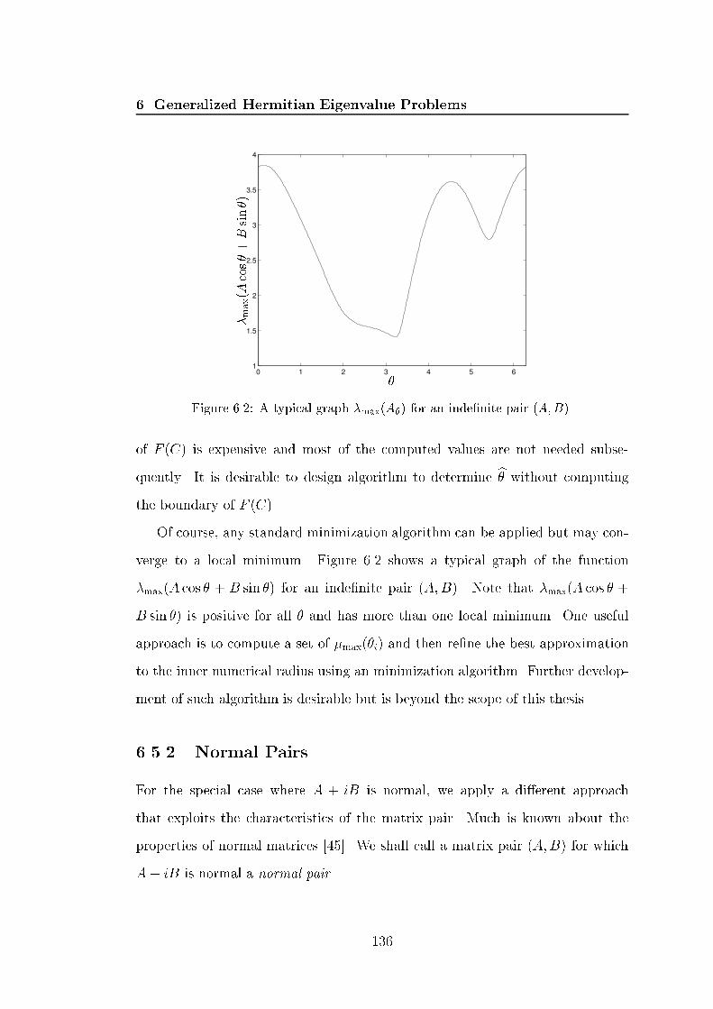
6. Generalized Hermitian Eigenvalue Problems

0 1 2 3 4 5 61

1.5

2

2.5

3

3.5

4

�� max(Acos�+Bsin�)

Figure 6.2: A typical graph �max(A�) for an inde�nite pair (A;B).of F (C) is expensive and most of the computed values are not needed subse-quently. It is desirable to design algorithm to determine b� without computingthe boundary of F (C).Of course, any standard minimization algorithm can be applied but may con-verge to a local minimum. Figure 6.2 shows a typical graph of the function�max(A cos � + B sin �) for an inde�nite pair (A;B). Note that �max(A cos � +B sin �) is positive for all � and has more than one local minimum. One usefulapproach is to compute a set of �max(�i) and then re�ne the best approximationto the inner numerical radius using an minimization algorithm. Further develop-ment of such algorithm is desirable but is beyond the scope of this thesis.6.5.2 Normal PairsFor the special case where A + iB is normal, we apply a di�erent approachthat exploits the characteristics of the matrix pair. Much is known about theproperties of normal matrices [45]. We shall call a matrix pair (A;B) for whichA+ iB is normal a normal pair. 136

6. Generalized Hermitian Eigenvalue ProblemsLemma 6.5.5 Let (A;B) be a normal pair. ThenA + iB is normal () A, B commute () AB is Hermitian:Proof: We have0 = (A + iB)�(A + iB)� (A+ iB)(A + iB)�= (A� iB)(A + iB)� (A+ iB)(A� iB)= (A2 + iAB � iBA +B2)� (A2 � iAB + iBA +B2)= 2i(AB �BA);which shows the �rst \()". Moreover, we have AB � BA = AB � B�A� =AB � (AB)�, which completes the proof. 2In addition, since normal matrices are always diagonalizable [45], we have thefollowing lemma.Lemma 6.5.6 If (A;B) is a normal pair then there exists a unitary Q such thatboth Q�AQ and Q�BQ are diagonal.Proof: Let C = A+iB have the spectral decomposition Q�Q� where QQ� =I and � is diagonal. We haveA = (C + C�)=2 =) Q�AQ = (�+ ��)=2;B = (C � C�)=2i =) Q�BQ = (�� ��)=2i;as required. 2One immediate consequence is as follows.Corollary 6.5.7 Let (A;B) be a normal pair. Then z is an eigenvector of A ifand only if z is an eigenvector of B. 2Lemma 6.5.6 provides the link between the eigenvalues of a normal pair (A;B)and those of A+ iB, as the following result shows.137

6. Generalized Hermitian Eigenvalue ProblemsLemma 6.5.8 Let (A;B) be a normal pair with eigenvalues �j for j = 1:n.Suppose A+ iB is nonsingular and has the spectral decompositionQ diag(r1ei�1 ; : : : ; rnei�n)Q�;where ri > 0. Then �j = 1= tan �j for j = 1:n.Proof: As in the proof of Lemma 6.5.6, we have Q�AQ = �A and Q�BQ =�B where �A = diag(�1; : : : ; �n) and �B = diag(�1; : : : ; �n). Thusdiag(r1ei�1 ; : : : ; rnei�n) = Q�(A+ iB)Q = �A + i�B:Then A� �B = Q(�A � ��B)Q� is singular, which implies� = �j�j = rj cos �jrj sin �j = 1tan �j :for some j, as required. 2When (A;B) is a normal pair, the �eld of values of A+ iB is the convex hullof the eigenvalues. Let A = B = ei�=4p2 diag(1;�1; i;�i): (6.19)From Figure 6.3, it is easily seen that d2(A;B; �) = �+ h = � +1=p2. Note thatthe �eld of values is an union of a set of triangles and h is easily computed usinga formula of Kahan [63], which is a numerically stable version of Heron's formulafor computing the area of a triangle. Kahan's formula also serves as an examplewhere computation with a guard digit is crucial to obtain a stable algorithm [39],[63].Let a, b, c be the lengths of the sides of the triangle and arrange a, b, c sothat a � b � c (which is the case in Figure 6.3). Then the area A of the triangleis given byA = 14q�a + (b+ c)��c� (a� b)��c+ (a� b)��a+ (b� c)�:138

6. Generalized Hermitian Eigenvalue Problems1

1

ImRe�1 0�1

c abhFigure 6.3: The �eld of values of normal pair (6:19).Since A also equals to 12ah, we haveh = 12aq�a + (b+ c)��c� (a� b)��c+ (a� b)��a+ (b� c)�:Note that the parentheses are essential [55]! Our algorithm for determiningd2(A;B; �) is simple. First compute the complete set of eigenvalues �k of A+iB 2C n�n , and arrange �k so that 0 � �p � �q < 2� for p < q, where �k denotes theangle between the positive real axis and the eigenvalue �k in the anti-clockwisedirection. Then there exists a subsequence f�kpg comprising the extreme pointsof F (A + iB). Calculate hkp for each triangle with vertices (0; �kp; �kp+1) with�kq+1 = �k1 . Then d2(A;B; �) = � +minkp hkp.Note that if �n � �1 < � and mini j�ij > 0 then (A;B) is a de�nite pair. If�n � �1 < � and mini j�ij = 0, or �n � �1 = �, then the origin is on the boundaryof the �eld of values F (A+ iB) and d2(A;B; �) = �6.6 Concluding RemarksWe have introduced the concept of the inner numerical radius. This importantquantity is related to the distance from an inde�nite matrix pair to the nearestde�nite pair, gives an alternative approach to determine whether a matrix is a139

6. Generalized Hermitian Eigenvalue Problemsde�nite pair, and can be used to determine the angle for rotating the matrixpair so that one of them is positive de�nite. It is desirable to derive e�cientalgorithms for �nding this quantity.For a normal pair, we presented an alternative approach for determining op-timal 2-norm perturbations using a formula of Kahan. This approach is numer-ically stable since the underlying formula is. An algorithm for determining thesubsequence of extreme points on the boundary of the �eld of values is underdevelopment.One open question is to generalize Theorem 6.5.4 for all unitarily invariantnorms.

140

Bibliography[1] Jan Ole Aasen. On the reduction of a symmetric matrix to tridiagonal form.BIT, 11:233{242, 1971.[2] E. Anderson, Z. Bai, C. H. Bischof, J. W. Demmel, J. J. Dongarra, J. J. DuCroz, A. Greenbaum, A. McKenney, S. Ostrouchov, and D. C. Sorensen.LAPACK Users' Guide, Release 2.0. Society for Industrial and AppliedMathematics, Philadelphia, PA, USA, 2nd edition, 1995.[3] E. Anderson and J. Dongarra. Evaluating block algorithm variants in LA-PACK. In J. Dongarra, P. Messina, D. Sorensen, and R. Voigt, editors, Pro-ceedings of the Fifth SIAM Conference on Parallel Processing for Scienti�cComputing, pages 1{8, Philadelphia, PA, USA, 1990. Society for Industrialand Applied Mathematics.[4] Peter Arbenz, Walter Gander, and Gene H. Golub. Restricted rank mod-i�cation of the symmetric eigenvalue problem: Theoretical considerations.Linear Algebra and Appl., 104:75{95, 1988.[5] Peter Arbenz and Gene H. Golub. On the spectral decomposition of Hermi-tian matrices modi�ed by low rank perturbations with applications. SIAMJ. Matrix Anal. Appl., 9(1):40{58, 1988.[6] Cleve Ashcraft, Roger G. Grimes, and John G. Lewis. Accurate symmetricinde�nite linear equation solvers. Manuscript, September 1995. To appearin SIAM J. Matrix Anal. Appl.[7] Victor Barwell and Alan George. A comparison of algorithms for solvingsymmetric inde�nite systems of linear equations. ACM Trans. Math. Soft-ware, 2(3):242{251, September 1976.141

Bibliography[8] �Ake Bj�orck. Numerical Methods for Least Squares Problems. Society forIndustrial and Applied Mathematics, Philadelphia, PA, USA, 1996.[9] A. J. Bosch. Note on the factorization of a square matrix into two Hermitianor symmetric matrices. SIAM Review, 29(3):463{468, September 1987.[10] Thierry Braconnier and Nicholas J. Higham. Computing the �eld of val-ues and pseudospectra using the Lanczos method with continuation. BIT,36(3):422{440, 1996.[11] James R. Bunch. Analysis of the diagonal pivoting method. SIAM J. Numer.Anal., 8(4):656{680, 1971.[12] James R. Bunch and Linda Kaufman. Some stable methods for calculatinginertia and solving symmetric linear systems. Math. Comput., 31:163{179,1977.[13] James R. Bunch, Christopher P. Nielsen, and Danny C. Sorensen. Rank-onemodi�cation of the symmetric eigenproblem. Numer. Math., 31:31{48, 1978.[14] James R. Bunch and Beresford N. Parlett. Direct methods for solving sym-metric inde�nite system of linear equations. SIAM J. Numer. Anal., 8:639{655, 1971.[15] David Carlson and Hans Schneider. Inertia theorems for matrices: Thesemide�nite case. J. Math. Anal. and Appl., 6(3):430{446, 1963.[16] S. Chandrasekaran, M. Gu, and A. H. Sayed. A stable and e�cient algorithmfor the inde�nite linear least-square problem. To appear in SIAM J. MatrixAnal. Appl., 1997.[17] Sheung Hun Cheng and Nicholas J. Higham. A modi�ed Cholesky algorithmbased on a symmetric inde�nite factorization. Numerical Analysis Report142

BibliographyNo. 289, Manchester Centre for Computational Mathematics, Manchester,England, April 1996. To appear in SIAM J. Matrix Anal. Appl.[18] Sheung Hun Cheng and Nicholas J. Higham. De�nite pairs and the innernumerical radius. Technical report in preparation, December 1997.[19] Moody T. Chu and Quanlin Guo. On the least squares approximation ofsymmetric-de�nite pencils subject to generalized spectral constraints. SIAMJ. Matrix Anal. Appl., 19(1):1{20, January 1998.[20] Andrew R. Conn, Nicholas I. M. Gould, and Philippe L. Toint. LANCELOT:A Fortran Package for Large-Scale Nonlinear Optimization (Release A).Springer Verlag, Berlin, Germany, 1992.[21] C. R. Crawford. Reduction of a band-symmetric generalized eigenvalue prob-lem. Comm. ACM, 16:41{44, 1973.[22] C. R. Crawford. A stable generalized eigenvalue problem. SIAM J. Numer.Anal., 13:854{860, 1976.[23] C. R. Crawford. Algorithm 646 PDFIND: A routine to �nd a positive de�-nite linear combination of two real symmetric matrices. ACM Trans. Math.Software, 12(3):278{282, September 1986.[24] C. R. Crawford and Yiu Sang Moon. Finding a positive de�nite linear com-bination of two Hermitian matrices. Linear Algebra and Appl., 51:37{48,1983.[25] J. J. M. Cuppen. A divide and conquer method for the symmetric tridiagonaleigenproblem. Numer. Math., 36:177{195, 1981.[26] James W. Demmel. Applied Numerical Linear Algebra. Society for Industrialand Applied Mathematics, Philadelphia, PA, USA, 1997.143

Bibliography[27] James W. Demmel, Inderjit Dhillon, and Huan Ren. On the correctnessof some bisection-like parallel eigenvalue algorithms in oating point arith-metic. Electronic Transactions on Numerical Analysis, 3:116{149, 1995.[28] J. E. Dennis, Jr. and D. J. Woods. Optimization on microcomputers:The Nelder-Mead simplex algorithm. In A. Wouk, editor, New ComputingEnvironments: Microcomputers in Large-Scale Computing, pages 116{122,Philadelphia, PA, USA, 1987. Society for Industrial and Applied Mathemat-ics.[29] J. J. Dongarra, J. R. Bunch, C. B. Moler, and G. W. Stewart. LINPACKUsers' Guide. Society for Industrial and Applied Mathematics, Philadelphia,PA, USA, 1979.[30] Bernd Fischer, Alison Ramage, David J. Silvester, and Andrew J. Wathen.Minimum residual methods for augmented systems. Mathematics ResearchReport 15, Department of Mathematics, University of Strathclyde, Glasgow,Scotland, June 1995.[31] R. Fletcher. Practical Methods of Optimization. John Wiley and Sons, Chich-ester, England, 2nd edition, 1987.[32] Anders Forsgren and Philip E. Gill. Primal-dual interior methods for non-convex nonlinear programming. Technical Report NA 96-3, Department ofMathematics, University of California, San Diego, USA, May 1996.[33] Anders Forsgren, Philip E. Gill, and Joseph R. Shinnerl. Stability of sym-metric ill-conditioned systems arising in interior methods for constrainedoptimization. SIAM J. Matrix Anal. Appl., 17(1):187{211, 1996.144

Bibliography[34] Anders Forsgren and Walter Murray. Newton methods for large-scale linearequality constrained minimization. SIAM J. Matrix Anal. Appl., 14(2):560{587, 1993.[35] F. G. Frobenius. Ueber die mit einer Matrix vertauschbaren Matrizen.Sitzungsberichte der K�oniglich Preusischen Akademie der Wissenschaften zuBerlin, pages 3{15, 1910.[36] Philip E. Gill and Walter Murray. Newton-type methods for unconstrainedand linearly constrained optimization. Math. Prog., 7:311{350, 1974.[37] Philip E. Gill, Walter Murray, and Margaret H. Wright. Practical Optimiza-tion. Academic Press, London, England, 1981.[38] Philip E. Gill, Michael A. Saunders, and Joseph R. Shinnerl. On the stabil-ity of cholesky factorization for symmetric quaside�nite systems. SIAM J.Matrix Anal. Appl., 17(1):35{46, 1996.[39] David Goldberg. What every computer scientist should know about oating-point arithmetic. ACM Computing Surveys, 23(1):5{48, 1991.[40] Gene H. Golub. Some modi�ed matrix eigenvalue problems. SIAM Review,15(2):318{334, 1973.[41] Gene H. Golub and Charles F. Van Loan. Matrix Computations. JohnsHopkins University Press, Baltimore, Maryland, USA, 2nd edition, 1989.[42] Nicholas I. M. Gould. On practical conditions for the existence and unique-ness of solutions to the general equality quadratic programming problem.Math. Prog., 32:90{99, 1985.145

Bibliography[43] Nicholas I. M. Gould. On the accurate determination of search directions forsimple di�erentiable penalty functions. IMA J. Numer. Anal., 6:357{372,1986.[44] Nicholas I. M. Gould. Constructing appropriate models for large-scale,linearly-constrained, nonconvex, nonlinear optimization algorithms. ReportRAL-95-037, Rutherford Appleton Labortory, Didcot, Oxon, UK, August1995.[45] Robert Grone, Charles R. Johnson, S�a, and Henry Wolkowicz. Normal ma-trices. Linear Algebra and Appl., 87:213{225, 1987.[46] Ming Gu and Stanley C. Eisenstat. A stable and e�cient algorithm for therank-one modi�cation of the symmetric eigenproblem. SIAM J. Matrix Anal.Appl., 15(4):1266{1276, 1994.[47] P. R. Halmos. Positive approximants of operators. Indiana Univ. Math. J.,21:951{960, 1972.[48] Richard J. Hanson. Aasen's method for linear systems with self-adjoint ma-trices. Visual Numerics, Inc., http://www.vni.com/books/whitepapers/Aasen.html, July 1997.[49] Emilie V. Haynsworth and Alexander M. Ostrowski. On the inertia of someclasses of partitioned matrices. Linear Algebra and Appl., 1:299{316, 1968.[50] Desmond J. Higham and Nicholas J. Higham. Structured backward error andcondition of generalized eigenvalue problems. Numerical Analysis ReportNo. 297, Manchester Centre for Computational Mathematics, Manchester,England, November 1996.[51] Nicholas J. Higham. Computing a nearest symmetric positive semide�nitematrix. Linear Algebra and Appl., 103:103{118, 1988.146

Bibliography[52] Nicholas J. Higham. FORTRAN codes for estimating the one-norm of a realor complex matrix, with applications to condition estimation (Algorithm674). ACM Trans. Math. Software, 14(4):381{396, December 1988.[53] Nicholas J. Higham. Optimization by direct search in matrix computations.SIAM J. Matrix Anal. Appl., 14(4):317{333, April 1993.[54] Nicholas J. Higham. The Test Matrix Toolbox for Matlab (version 3.0).Numerical Analysis Report No. 276, Manchester Centre for ComputationalMathematics, Manchester, England, September 1995.[55] Nicholas J. Higham. Accuracy and Stability of Numerical Algorithms. Societyfor Industrial and Applied Mathematics, Philadelphia, PA, USA, 1996.[56] Nicholas J. Higham. Recent developments in dense numerical linear algebra.In I. S. Du� and G. A. Watson, editors, The State of the Art in NumericalAnalysis, volume 22, pages 1{26, Oxford, England, 1997. Oxford UniversityPress.[57] Nicholas J. Higham. Stability of Aasen's method. Manuscript, 1997.[58] Nicholas J. Higham. Stability of the diagonal pivoting method with partialpivoting. SIAM J. Matrix Anal. Appl., 18(1):52{65, January 1997.[59] Nicholas J. Higham and Sheung Hun Cheng. Modifying the inertia of matri-ces arising in optimization. Numerical Analysis Report No. 295, ManchesterCentre for Computational Mathematics, Manchester, England, September1996. To appear in Linear Algebra and Appl.[60] Roger A. Horn and Charles R. Johnson. Matrix Analysis. Cambridge Uni-versity Press, Cambridge, England, 1985.147

Bibliography[61] Roger A. Horn and Charles R. Johnson. Topics in Matrix Analysis. Cam-bridge University Press, Cambridge, England, 1991.[62] Institute of Electrical and Electronics Engineers, New York. IEEE Standardfor Binary Floating-Point Arithmetic, ANSI/IEEE Standard 754-1985, 1985.Reprint in SIGPLAN Notices, 22(2):9{25, 1987.[63] W. Kahan. How Cray's arithmetic hurts scienti�c computation (and whatmight be done about it). Manuscript prepared for the Cray User Groupmeeting in Toronto, June 1990.[64] Ren-Cang Li. A perturbation bound for de�nite pencils. Linear Algebra andAppl., 179:191{202, 1993.[65] The MathWork, Inc., Natick, MA, USA. MATLAB User's Guide, 1992.[66] W. Miller and C. Spooner. Software for roundo� analysis, II. ACM Trans.Math. Software, 4:369{387, 1978.[67] Jorge J. Mor�e and Danny C. Sorensen. On the use of directions of negativecurvature in a modi�ed Newton's method. Math. Prog., 16:1{20, 1979.[68] W. Oettli and W. Prager. Compatibility of approximate solution of linearequations with given error bounds for coe�cients. Numer. Math., 6:405{409,1964.[69] A. M. Ostrowski. A quantitative formulation of Sylvester's law of inertia.Proc. Nat. Acad. Sci. U.S.A., 45:740{744, 1959.[70] B. N. Parlett and H. C. Chen. Use of inde�nite pencils for computing dampednatural modes. Linear Algebra and Appl., 140:53{88, 1990.[71] Beresford N. Parlett. The Symmetric Eigenvalue Problem. Prentice-Hall,Englewood Cli�s, NJ, USA, 1980.148

Bibliography[72] Beresford N. Parlett. Symmetric matrix pencils. J. Comp. and Appl. Math.,38:373{385, 1991.[73] Alex Pothen. Predicting the structure of sparse orthogonal factors. LinearAlgebra and Appl., 192:183{203, 1993.[74] J. D. Pryce. Numerical Solution of Strum{Liouville Problems. Oxford Uni-versity Press, Oxford, England, 1993.[75] H. Rutishauser. On Jacobi rotation patterns. In Proc. of Symposia in Appl.Math., volume 15, pages 219{239, Providence, R.I., 1963. American Mathe-matical Society.[76] Michael A. Saunders. Solution of sparse rectangular systems using LSQRand CRAIG. BIT, 35:588{604, 1995.[77] Tamar Schlick. Modi�ed Cholesky factorizations for sparse preconditioners.SIAM J. Sci. Comput., 14:424{445, 1993.[78] Robert B. Schnabel and Elizabeth Eskow. A new modi�ed Cholesky factor-ization. SIAM J. Sci. Stat. Comput., 11(6):1136{1158, 1990.[79] David J. Silvester and Andrew J. Wathen. Fast and robust solvers for time-discretised incompressible Navier{Stokes equations. In D.F. Gri�ths andG. A. Watson, editors, Numerical Analysis 1995, Proceedings of the 16thDundee Conference, volume 344 of Pitman Research Notes in Mathematics,pages 154{168, Essex, England, 1996. Longman Scienti�c and Technical.[80] Robert D. Skeel. Scaling for numerical stability in Gaussian elimination. J.Assoc. Comput. Mach., 26(3):494{526, 1979.[81] G. W. Stewart. Introduction to Matrix Computations. Academic Press, NewYork, 1973. 149

Bibliography[82] G. W. Stewart. Perturbation bounds for the de�nite generalized eigenvalueproblem. Linear Algebra and Appl., 23:69{85, 1979.[83] G. W. Stewart. The e�cient generation of random orthogonal matrices withan application to condition estimators. SIAM J. Numer. Anal., 17:403{409,1980.[84] G. W. Stewart and Ji-guang Sun. Matrix Perturbation Theory. AcademicPress, London, England, 1990.[85] Olga Taussky. The role of symmetric matrices in the study of general ma-trices. Linear Algebra and Appl., 5:147{154, 1972.[86] V. J. Torczon. Multi-directional search: A direct search algorithm for parallelmachines. PhD thesis, Rice University, Houston, Texas, USA, 1989.[87] V. J. Torczon. On the convergence of the multidirectional search algorithm.SIAM J. Optimization, 1:123{145, 1991.[88] H. P. M. v. Kempen. Variation of the eigenvalues of a special class of Her-mitian matrices upon variation of some of its elements. Linear Algebra andAppl., 3:263{273, 1970.[89] Robert J. Vanderbei. Symmetric quasi-de�nite matrices. SIAM J. Optimiza-tion, 5(1):100{113, 1995.[90] Visual Numerics, Inc., Houston, TX, USA. IMSL Fortran 90 MP Library,1996. Part Number 3743, p. 9.[91] J. H. Wilkinson. Global convergence of tridiagonal QR algorithm with originshifts. Linear Algebra and Appl., 1:409{420, 1968.[92] Harald K. Wimmer. On Ostrowski's generalization of Sylvester's law ofinertia. Linear Algebra and Appl., 52/53:739{741, 1983.150