computing upper and lower bounds on linear functional
TRANSCRIPT

Computing Upper and Lower Bounds on LinearFunctional Outputs from Linear Coercive Partial
Differential Equations
by
Alexander M. Sauer-Budge
S.M., Massachusetts Institute of Technology, 1998B.S., University of California, Davis, 1996
SUBMITTED TO THE DEPARTMENT OF AERONAUTICS AND ASTRONAUTICS
IN PARTIAL FULFILLMENT OF THE REQUIREMENTS FOR THE DEGREEOF
DOCTOR OF PHILOSOPHY IN AERONAUTICS AND ASTRONAUTICS
AT THE
MASSACHUSETTS INSTITUTE OF TECHNOLOGY
2003 SEPTEMBER
© Massachusetts Institute of Technology September. All rights reserved.
-. 4
A uthor .............................
C ertified by ........................
Certified by ...................
Certified by .........
Associa
Accepted by....... ...... . .
H.N. Slat
............................................Department of Aeronautics and Astronautics
j A August 1, 2003
.$.. ..9 ... . s . .... ... .. . . ........Jaime Peraire
Professor of Aeronautics and AstronauticsThesis Supervisor
. . .. .........................-- -.......Anthony T. Patera
Prpfqssor of Mechanic4 Engineering
+Dvid L. Darmofalte Professor of Aeronauti and Astronautics
.ard 1M. Greitzerer Professor of Aeronautics and Astronautics
Chair, Committee on Graduat SggwHyOF TE
NOV
LIB
3EUS INSTITUTESETTS INSTITUTECHNOLOGY
0 5 2003
RARIES
a A A --%

2

3
Computing Upper and Lower Bounds on Linear FunctionalOutputs from Linear Coercive Partial Differential
Equations
by
Alexander M. Sauer-Budge
Submitted to the Department of Aeronautics and Astronauticson August 1, 2003, in partial fulfillment of the
requirements for the degree ofDoctor of Philosophy in Aeronautics and Astronautics
Abstract
Uncertainty about the reliability of numerical approximations frequently undermines theutility of field simulations in the engineering design process: simulations are often nottrusted because they lack reliable feedback on accuracy, or are more costly than neededbecause they are performed with greater fidelity than necessary in an attempt to bolstertrust. In addition to devitalized confidence, numerical uncertainty often causes ambigu-ity about the source of any discrepancies when using simulation results in concert withexperimental measurements. Can the discretization error account for the discrepancies,or is the underlying continuum model inadequate?
This thesis presents a cost effective method for computing guaranteed upper andlower bounds on the values of linear functional outputs of the exact weak solutions tolinear coercive partial differential equations with piecewise polynomial forcing posed onpolygonal domains. The method results from exploiting the Lagrangian saddle pointproperty engendered by recasting the output problem as a constrained minimizationproblem. Localization is achieved by Lagrangian relaxation and the bounds are com-puted by appeal to a local dual problem. The proposed method computes approximateLagrange multipliers using traditional finite element discretizations to calculate a pri-mal and an adjoint solution along with well known hybridization techniques to calcu-late interelement continuity multipliers. At the heart of the method lies a local dualproblem by which we transform an infinite-dimensional minimization problem into afinite-dimensional feasibility problem.
The computed bounds hold uniformly for any level of refinement, and in the asymp-totic convergence regime of the finite element method, the bound gap decreases at twicethe rate of the 'H -norm measure of the error in the finite element solution. Given a finiteelement solution and its output adjoint solution, the method can be used to provide acertificate of precision for the output with an asymptotic complexity that is linear in the

4
number of elements in the finite element discretization. The complete procedure com-putes approximate outputs to a given precision in polynomial time. Local informationgenerated by the procedure can be used as an adaptive meshing indicator. We apply themethod to Poisson's equation and the steady-state advection-diffusion-reaction equation.
Thesis Supervisor: Jaime Peraire
Title: Professor of Aeronautics and Astronautics

5
Acknowledgments
First and foremost, I would like to thank my advisor, Professor Jaime Peraire,for his constant vision and continual supply of ideas, as well as for his encour-agement and patience during the course of this research. Second, I would like toheartily thank Professor Anthony Patera for taking me under his wing during myadvisor's sabbatical and for introducing me to functional analysis in the contextof the finite element method. I would like to thank everyone who participatedin the "bounds sessions" organized by Professor Patera. In particular, I wouldlike to thank Luc Machiels, Dimitrios Rovas, Ivan Oliveira, Karen Veroy, andChristophe Prud'homme for everything that they taught me as well as for theircamaraderie. I would like to thank Professor Gilbert Strang for opening my mindto the underlying beauty of mathematics, and then Professor Dimitris Bertsimasto the underlying mathematical beauty of decision making. I would like to thankmy committee as a whole, Professors Jaime Peraire, Anthony Patera, David Dar-mofal, and Dimitris Bertsimas for their helpful comments and insight. Further, Iwould like to thank Javier Bonet, Antonio Huerta, and Robert Freund for helpfuldiscussions of various aspects of the method proposed in this thesis. As this workcould not have been completed without financial support, I would also like tothank Thomas A. Zang for the support provided through NAG-1-1978 and theSingapore-MIT Alliance. I could not have overcome the many frustrations anddisappointments experienced during the course of my studies without the unwa-vering support of my family and friends. I would especially like to thank mywife, Alexis, and my parents, Roger and Leslee Budge, whose constant love andencouragement renewed my strength when I thought that I could not continue.Finally, I would like to thank my Lord and Savior, Jesus Christ, for setting mefree from a life of vanity and for teaching my heart, mind, body, and spirit notonly about the wonders of grace, peace, faith, and hope, but about the very thingfor which we were created- to love and be loved.

6

Contents
1 Introduction1.1 Techniques for Reliability Assessment . . . .
1.1.1 Recovery Based Error Estimators .1.1.2 Residual Based Error Estimators
1.1.2.1 Explicit Estimators . . . . .1.1.2.2 Implicit Estimators . . . . .1.1.2.3 Summary of Residual Based
1.1.3 Relation to Other Methods . . . . . .1.2 Overview . . . . . . . . . . . . . . . . . . . .
2 Energy Bounds for Poisson's Equation2.1 An Intrinsic Minimization Principle . . . . .2.2 Weak Continuity Reformulation . . . . . . .2.3 Localization by Continuity Relaxation . . .
2.3.1 Continuity Multiplier Approximation2.4 Local Dual Subproblem . . . . . . . . . . . .
2.4.1 Subproblem Computation . . . . . .2.5 Energy Bound Procedure . . . . . . . . . . .
2.5.1 Properties of the Energy Bound . . .2.6 Numerical Results . . . . . . . . . . . . . . .
3 Output Bounds For Poisson's Equation3.1 Weak Continuity Reformulation . . . . . . .3.2 Localization by Continuity Relaxation . . .
3.2.1 Lagrange Multiplier Approximation .3.3 Local Dual Subproblem . . . . . . . . . . . .
3.3.1 Subproblem Computation . . . . . .3.4 Output Bound Procedure . . . . . . . . . .
3.4.1 Properties of the Output Bounds . .3.4.2 Computational Complexity . . . . . .
13. . . . . . . . . . . . 16. . . . . . . . . . . . 17. . . . . . . . . . . . 18. . . . . . . . . . . . 19. . . . . . . . . . . . 23Error Estimators . . 26. . . . . . . . . . . . 26. . . . . . . . . . . . 28
30. . . . . . . . . . . . 3 1. . . . . . . . . . . . 32. . . . . . . . . . . . 34. . . . . . . . . . . . 34. . . . . . . . . . . . 36. . . . . . . . . . . . 39. . . . . . . . . . . . 4 1. . . . . . . . . . . . 4 2. . . . . . . . . . . . 4 6
48. . . . . . . . . . . . 4 9. . . . . . . . . . . . 50. . . . . . . . . . . . 5 1. . . . . . . . . . . . 53. . . . . . . . . . . . 55. . . . . . . . . . . . 5 7. . . . . . . . . . . . 59. . . . . . . . . . . . 60
7

CONTENTS
3.5 Adaptive Refinement ......................... 623.6 Numerical Results ........................... 63
3.6.1 Uniformly Forced Square Domain . . . . . . . . . . . . . . 643.6.2 Linearly Forced Square Domain . . . . . . . . . . . . . . . 653.6.3 Unforced Corner Domain . . . . . . . . . . . . . . . . . . . 68
4 Output Bounds for the ADR Equation 714.1 Constrained Minimization Reformulation . . . . . . . . . . . . . . 73
4.1.1 Weak Continuity . . . . . . . . . . . . . . . . . . . . . . . 734.1.2 Operator Decomposition . . . . . . . . . . . . . . . . . . . 744.1.3 Constrained Minimization Statement . . . . . . . . . . . . 754.1.4 Localization by Lagrangian Relaxation . . . . . . . . . . . 76
4.1.4.1 Lagrange Multiplier Approximation . . . . . . . . 774.2 Elemental Subproblems . . . . . . . . . . . . . . . . . . . . . . . . 79
4.2.1 Dualization of Local Minimization . . . . . . . . . . . . . . 814.2.2 Dual Subproblems . . . . . . . . . . . . . . . . . . . . . . 844.2.3 Subproblem Computation . . . . . . . . . . . . . . . . . . 87
4.3 Output Bound Procedure . . . . . . . . . . . . . . . . . . . . . . 894.4 Numerical Examples . . . . . . . . . . . . . . . . . . . . . . . . . 92
4.4.1 Quasi-2D Transport . . . . . . . . . . . . . . . . . . . . . 934.4.2 Rotating Transport . . . . . . . . . . . . . . . . . . . . . . 96
5 Conclusion 1015.1 Contribution . . . . . . . . . . . . . . . . . . . . . . . . . . . . . . 1015.2 Recommendations. . . . . . . . . . . . . . . . . . . . . . . . . . . 104
A Equilibration Procedure 107A.1 Problem Statement . . . . . . . . . . . . . . . . . . . . . . . . . . 107A .2 Prelim inaries . . . . . . . . . . . . . . . . . . . . . . . . . . . . . 108A .3 Subproblem s . . . . . . . . . . . . . . . . . . . . . . . . . . . . . . 110
Bibliography
8
115

List of Figures
2.6.1 Uniformly forced square domain convergence history. . . . . . . . 47
3.6.1 Uniformly forced square domain convergence history. . . . . . . . 653.6.2 The dependency of flow rate through a viscous duct on channel
h eight. . . . . . . . . . . . . . . . . . . . . . . . . . . . . . . . . . 663.6.3 Linearly forced square domain convergence history. . . . . . . . . 673.6.4 Unforced corner domain convergence history. . . . . . . . . . . . . 683.6.5 Unforced corner domain adaptive solutions, local indicators and
m eshes. . . . . . . . . . . . . . . . . . . . . . . . . . . . . . . . . 70
4.4.1 Quasi-2D uniform refinement results with q = 1, a = 10 and y = 10. 954.4.2 Quasi-2D transport adaptive solutions, local indicators and meshes. 984.4.3 Rotational transport forcing and output regions. . . . . . . . . . . 994.4.4 Rotating transport uniform refinement results. . . . . . . . . . . . 994.4.5 Rotating transport adaptive solutions, local indicators and meshes. 100
A.3.1Equilibration subproblem interior case. . . . . . . . . . . . . . . . 111A.3.2Equilibration subproblem boundary cases. . . . . . . . . . . . . . 113
9

10 LIST OF FIGURES
List of Tables
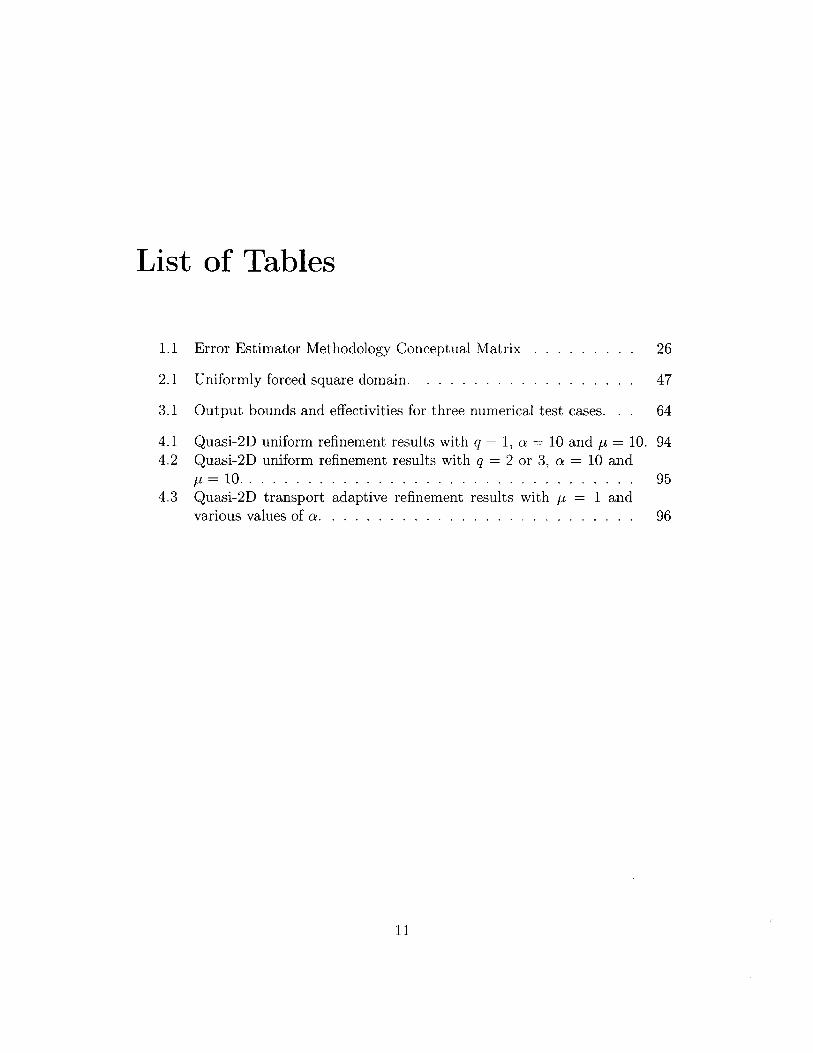
1.1 Error Estimator Methodology Conceptual Matrix . . . . . . . . . 26
2.1 Uniformly forced square domain. . . . . . . . . . . . . . . . . . . 47
3.1 Output bounds and effectivities for three numerical test cases. . . 64
4.1 Quasi-2D uniform refinement results with q = 1, a = 10 and t = 10. 944.2 Quasi-2D uniform refinement results with q = 2 or 3, a = 10 and
y = 10 . . . . . . . . . . . . . . . . . . . . . . . . . . . . . . . . . . 954.3 Quasi-2D transport adaptive refinement results with p = 1 and
various values of a. . . . . . . . . . . . . . . . . . . . . . . . . . . 96
11

12 LIST OF TABLES

Chapter 1
Introduction
Uncertainty about the reliability of numerical approximations frequently under-
mines the utility of field simulations in the engineering design process: simula-
tions are often not trusted because they lack reliable feedback on accuracy, or are
more costly than necessary because they are performed with greater fidelity than
necessary in an attempt to bolster trust. In addition to devitalized confidence,
numerical uncertainty often causes ambiguity about the source of any discrepan-
cies when using simulation results in concert with experimental measurements.
Can the discretization error account for the discrepancies, or is the underlying
continuum model inadequate?
To disambiguate, we define precision to be the conformity of a simulation re-
sult to the exact solution of the continuum model, and we define accuracy to be
the conformity of a simulation result to the physical fact. Three essential questions
must be answered before a simulation result can be trusted and effectively used in
the making important decisions. Do the mathematical equations model the rele-
vant phenomena? Does the software actually solve the discretized mathematical
13

CHAPTER 1. INTRODUCTION
model? Does the simulation result contain sufficient precision to be considered a
solution of the mathematical model?
The verification and validation process has emerged to help answer these ques-
tions [AIA98, OT02, SWCP01]. Verification ensures that the simulation repro-
duces known analytical results and trusted benchmarks, while validation ensures
that the simulation results agree with trusted experimental data. The former con-
firming that the simulation software solves the discretized mathematical model
with sufficient precision for the verification test cases, and the latter substantiat-
ing the capacity of the mathematical model to represent the relevant phenomena
for the validation test cases. Verification and validation are necessary steps in
assessing the reliability of simulation results, but these steps alone do not certify
the accuracy of results for cases outside the test suite.
The reliability of every simulation result used in decision making should be
taken into account, but it is often prohibitively expensive to do so. A priori error
estimates inform us of the asymptotic rates of convergence, but cannot answer the
ever present engineering question, "can I trust the current approximation?" Such
questions often revolve around concerns of mesh fidelity and feature resolution
- issues of numerical uncertainty which erode confidence in the simulation. As
confidence erodes, so does the utility of the simulation in the engineering design
process: either the simulation is not trusted, or it is more costly than necessary.
While confidence in the precision of a field simulation can be buoyed by per-
forming convergence studies, such studies are computationally very expensive and
in practice are often not performed at more than a few conditions, if at all, due to
cost and time constraints. For this reason, researchers and practitioners employ
14

15
adaptive methods to converge the solution in a manner that costs less in time and
resources than uniform refinement. Adaptive methods powered by current error es-
timation technology {Ver94, BKROO, BR78a, BSUG95b, BR96a, BBRW98, HR99,
RS97, RS99, SBD+00, VD03, VD02], however, provide only asymptotic guarantees
of precision, at best, and no guarantees of precision, at worse, since the conver-
gence of adaptive methods remains an open question [MNS02, BV84, Dor96].
Our observations of engineering practice inform us that integrated quantities
such as forces, total fluxes, average temperatures and displacements are frequently
queried quantitative outputs from field simulations and that design and analysis
does not always require the full precision available. In particular, we will restrict
our attention to integrated outputs defined by linear functionals, which depend
linearly on the solution field. The primary objective of our method, therefore, is
to certify the precision of integrated outputs for low fidelity simulations as well as
high fidelity simulations.
We call our bounds uniform to differentiate our goal of obtaining quantitative
bounds for all levels of refinement from the lesser goal of obtaining quantitative
bounds only asymptotically in the limit of refinement. In this regard, the com-
plete procedure can be viewed as a polynomial time algorithm in the number
of mesh elements that provides a certificate of precision for a predicted output.
The certificate guarantees a minimum level of precision in the output from a
particular finite-dimensional approximation with respect to the output from the
infinite-dimensional model that it is approximating. Furthermore, the procedure
provides local information that can be used in conjunction with adaptive meshing
to efficiently drive a solution to an arbitrary and guaranteed precision.

CHAPTER 1. INTRODUCTION
The method can answer the question "Does the simulation result contain suf-
ficient precision to be considered a solution of the mathematical model?" by
certifying the precision of integrated outputs from finite element simulations for
any level of mesh refinement. The method can help answer the question "Does the
software actually solve the discretized mathematical model?" because it has eas-
ily checkable preconditions to help verify correctness of the simulation software.
The quantification of numerical error removes uncertainty about the fidelity of
the discretization and aides the practitioner in distinguishing modeling error from
numerical error when validating the simulation and thus can aid in answering the
question "Do the mathematical equations model the relevant phenomena? ". In
particular, the method can invalidate mathematical models when the error bounds
returned by the method do not overlap with the experimental data. This can even
be done with relatively low fidelity simulations in cases of gross deviation of the
mathematical model from physical reality.
1.1 Techniques for Reliability Assessment
Verification and a posteriori error analysis have a long history in the development
of the finite element method with a plethora of different approaches forwarded
and investigated beginning with the pioneering work of Fraeijs de Veubeke in
the mid-1960s and early 1970s [Fra64, Fra65, FH72]. Although powerful, his
method was not practical because it required a global computation. In the late
1970s, Babuska and Rheinboldt initiated work on modern error estimation tech-
niques by proposing the first inexpensive method requiring only local computa-
'R78a, BR78b, BR81]. Ainsworth and Oden giv ummary account of
16

1.1. TECHNIQUES FOR RELIABILITY ASSESSMENT
the work on a posteriori error estimators in [A097], while Babuska, Strouboulis,
Updahyay and collaborators probe the quality and robustness of a number of con-
temporary error estimators in [BSUG97, BSUG94, BSUG95a, BSU+94, ZSB01]
with numerical experiments. Additional comparisons and descriptions of the more
popular methods can be found in [ODRW89, Zhu97, SH98, AC92, Ver94].
1.1.1 Recovery Based Error Estimators
Finite element a posteriori error estimators can be broadly classified as recovery
based methods or residual based methods, although evidence exists that some meth-
ods which appear distinct under this categorization are equivalent [Zhu97, ZZ99]
in special circumstances. Recovery based methods estimate the error in the energy
norm by comparing the native finite element solution with one enhanced through a
post-processing procedure. The post-processing procedure typically smoothes the
finite element solution or exploits special superconvergent properties of the dis-
cretization to obtain a recovered solution which is assumed to be more accurate
than the original. Zienkiewicz and Zhu first proposed recovery based methods in
the late 1980s [ZZ87] and have subsequently improved them [ZZ92a, ZZ92b] by ex-
ploiting superconvergence. Recovery based methods have experienced popularity
due to their simplicity as well as being very effective in practice [ZBS99, ZSBO1I].
Recovery based methods produce asymptotically exact error estimates when
the post-processing produces a superconvergent recovered solution [CB02]. Asymp-
totically exact error estimates converge to the exact error in the asymptotic limit
of mesh refinement, but do not provide any guarantees of one-sidedness required
for bounding the error. Asymptotic exactness is a very useful property for an error
17

CHAPTER 1. INTRODUCTION
estimator, but without uniform one-sidedness an error estimator cannot provide
confirmation of precision. Even if the error estimator produces reliable estimates
for a number of validation cases, there is little to assure the practitioner that the
estimate can be trusted for the case of interest. Such limitations relegate the error
estimator to serving as an oracle for balancing error contributions (of uncertain
magnitude) in mesh adaptivity, and undermine their effectiveness as methods for
confirmation and building adaptive meshes with guaranteed error tolerances.
1.1.2 Residual Based Error Estimators
Residual based methods, like the first locally computed error estimators which
were introduced by Babuska and Rheinboldt, estimate the error in the energy
norm either from an explicit evaluation of the local residual or by solving an
implicit relationship with the local residual as the data. The majority of the
work on error estimation has focused on residual based methods and the method
proposed by this thesis can be categorized as such a method. Consider the simple
model problem for an unknown real scalar field variable u and some nonnegative
scalar coefficient y and data f posed on a two-dimensional domain
-Au + pU = f in Q C R2
subject only to homogeneous Dirichlet boundary conditions. The variational-weak
statement follows as: find u in R'(Q)
a(u, v) = e(v), Vv E (1(1))
18
(1.1.1)

1.1. TECHNIQUES FOR RELIABILITY ASSESSMENT
where
a(u, v) = Vu -Vv + puv dQ,
and
f(v) = jfvdQ.
The operator a : V(Q) x X-(Q) is symmetric, bilinear, continuous and coercive.
We have introduced the usual Hilbert space
-H1() = { v v E £ 2 (Q), Vv E (E2(Q))d
where d is the number of physical dimensions and
2 (Q V IV12 dQ < +oo
is the space of square integrable functions on Q.
1.1.2.1 Explicit Estimators
Many of the first residual based a posteriori error estimators computed an error
indicator explicitly from the approximate solution, without solving any additional
problems [BR79, KGZB83, BM87]. Following Ainsworth and Oden [A097], we
can build an explicit error estimator for the above model problem by the so called
error equation or residual equation
a(e, v) = a(u, v) - a(uh, v) = f(v) - a uh, v), VV E (1.()),
19
(1.1.2)

20 CHAPTER 1. INTRODUCTION
in which the error is defined as e - u - uh, where Uh E Vh is a finite element
approximation to the solution on some triangulation of the domain, Th. The error
equation expands to
a(e, v) = j fV - VUhVV - IUhv dQ, Vv E H'(Q).T ETh T
Assuming Uh to be in H 2 (Q) and integrating by parts over the elements decom-
poses the error equation into local error contributions from each element
a(e, v) = E rvdQ - VUh - nv dF Vv (E H(Q),T En E T faT0
where r f + Auh - pUh and n is the unit outward normal vector to 9Th. The
trace of v is continuous along an edge, which allows the last term of the previous
equation to be written as the jump discontinuity in the approximation to the flux.
a(e, v) - rv dQ - > [Vuh - n] v dF, Vv E H1(Q),TGThJ -Y9h\9 f
where
[VUa - n] = VuhIT+ - n + VUhT - = -R
is the jump discontinuity in the flux. We can now write
a(e, v) =Z rvdQ + Rv dl.T E~ T 8 Q

1.1. TECHNIQUES FOR RELIABILITY ASSESSMENT
Galerkin orthogonality, a(e, vh) = 0, Von E Vh, implies that
0 = Zjrvv dQ + E fRvhv dr,TET -T E
where LVh -H 1(T) -* Vh(T) is the linear operator that projects the members
of the infinite-dimensional continuous space, 7-(T), onto the finite-dimensional
approximation subspace, Vh(T). We can subtract the previous two equations to
obtain
a(e, v) = r(v - vhv) dQ + R(v - Hvhv) df, Vv E H (Q).TET T Th J
Applying the Cauchy-Schwartz Inequality gives
a(e, v) ||r 1|2(T) I I Hv lVftI2(T)TETh
+ ||2 || - Hv oI L2(, Vv E XMG)yETh
Interpolation theory [Cia78, QV971 informs us that there exists a constant C which
is independent of v and h, the diameter of the element, such that
l|v - UvhvLe2 (T) < ChvI7- (T*),
||v - flvhVllL 2(,) ChiVl(T*),
where T* denotes the subdomain consisting of all elements sharing a common edge
with element T, and h is the diameter of T. Inserting these estimates into the
21

CHAPTER 1. INTRODUCTION
previous equation and absorbing the various constants, yields
a(e,v) < CjvfH1(Q) h2 |Ir|12 (T) + ( h||R||12h)}-TETh -YE a7h
Finally, recalling that IVol ( ) < a(v, v), an a posteriori error estimate can be
written
a(e,e) C { h2||r|12(T) + ( h||R|12) .T ETh -yE'Th
Both interior and edge residual quantities comprise the estimate, but in many
situations the edge contribution dominates the estimate [KVOO, CV99].
Although simple, explicit error estimators of this sort have two obvious draw-
backs. First and foremost, the estimate contains a generic unknown constant
which renders the estimate useless for certifying the absolute precision of a nu-
merical result. Second, the quantity on the right estimates the error in the energy
norm measure which may or may not be relevant to particular decision for which
the simulation was undertaken.
Linear Functional Output Error Measure An explicit estimator in a lin-
ear functional output can be bootstrapped from the above energy estimator and
an output adjoint. These estimators, of course, still contain unknown constants
which make them unsuitable for confirmation and validation, but by serving as in-
dicators for mesh adaptivity they can be used to improve the efficiency with which
engineering quantities of interest can be approximated with greater precision.
Defining a linear continuous output functional f' : V -+ R. First, find Oh E Vh
22

1.1. TECHNIQUES FOR RELIABILITY ASSESSMENT
such that
a(0h, vh) = (Vh), Vo E Ph. 113
Galerkin orthogonality and the Cauchy-Schwarz Inequality allow us to write
EG(e) = a(e, @) = a(e, 0 - 0h) e C y~evh h1' - IhJJvh, (1.1.4)
where the solution error lJeJVh was obtained above. A bound on the term ||$ -
Oh!IVh, where 4 E H'(Q) is the exact adjoint defined as
a(@, v) = 0 (v), Vv E (),
can be obtained in an analogous manner to the solution error. This equation
gives a lower bound, an upper bound can be found with the same process, but by
solving for -ED.
1.1.2.2 Implicit Estimators
The simplicity and low computational cost of explicit estimators makes them
attractive despite their lack of quantitative feedback, while the quantitative po-
tential of implicit estimators makes them attractive despite their additional cost.
That implicit estimators are typically formulated without explicit constants, how-
ever, belies the fact that the vast majority of such estimators tacitly depend on
uncomputable quantities which must be approximated in a vitiating manner. As
a result, existing implicit estimators cannot be used with confidence to validate
the precision of a simulation result, despite the additional cost of such estimators.
An implicit estimator for the error in a linear functional output can be con-
23

CHAPTER 1. INTRODUCTION
structed from the error equation (1.1.2) using the approximate working solution
Uh and the approximate adjoint Oh previously introduced. In order to reduce the
computational cost of the resulting estimator, we introduce a domain decomposi-
tion by partitioning the domain with the finite element triangulation, Th. On the
aggregate of elements, which we call the broken domain, we define a broken space
V = HTETh 7 (T) and a continuity bilinear form b : V x A constructed so that
V() = {E V(Q) b(, A) = 0, VA E A ,
where A is the space of bounded linear edge functions (the dual of the trace space
of 7-(T)). Introducing the domain decomposition allows us to localize the error
estimator computation to a single element.
After computing Uh and ih with standard methods, we can compute equili-
brating fluxes Au and A0 by solving the equations
b( , Au) = E(0) - a(Uh, 0), VWE 4
b(0,A') = - 0 (i) -a(,@bh), Vi E Vh,
using well established and inexpensive equilibration techniques. Equilibrating lo-
calization techniques like this are an important ingredient to formulating robust
and asymptotically exact implicit error estimators [AO93a, Ain96, ABF99, A097,
BW851.
By choosing a high fidelity finite-dimensional approximation space V, (T) which
we assume can safely be a surrogate for the infinite-dimensional space N 1 (T), we
24

1.1. TECHNIQUES FOR RELIABILITY ASSESSMENT
can solve a pair of high fidelity reconstructed error problems on each element
2a(eu, v) = f(v) - a(uh, v) - b(v, Au), Vv E V,(T),
2a(el, v) = -E2(v) - a(v,'h) - b(v, AO), Vv E V,(T).
Upper and lower bounds on the output s - f 0 (u) can then be computed from the
expression
s = 1i(u) - 2 1: a(e',e) ± 2 ( a(e,er) 1
TGTh T E T T ET ) T )
The quantities s* are quantitative bounds on the output from the hypothetical
global high fidelity solution u,: s;- < 20 (u) < s+.
The method we have outlined here follows that of Patera, Paraschivoiu, Peraire,
et al. [PPP97, PP98, MPP99, PPOO, BP02] in which the high fidelity approxima-
tion space V, (T) is an h-refinement of the local element subdomain. As the method
uses both a working mesh and "truth" mesh, it also falls under a category of two-
level finite element methods studied by Brezzi and Marini [BM02]. Methods by
other workers in the field have a similar character but use p-refinement for the
local enriched approximation. Numerous implicit error estimation methods fall
into this overarching scheme of computing high fidelity reconstructed errors from
a localized working approximation. They differentiate themselves by the methods
they choose for each step and how they measure the error. For instance, flux-free
local problems may be computed on a patch of elements resulting from a partition
of unity [MMPOO, BPP01], or the error might be measured with respect to the
constitutive law [LadOO, LR97, LL83].
25

CHAPTER 1. INTRODUCTION
What the methods all have in common is substitution of a computable finite-
dimensional problem where an uncomputable infinite-dimensional problem is re-
quired to guarantee bounds [AK01, A093b, BSG99, SBG00]. Error estimates that
do not have the guarantee of one-sidedness, or that approach exactness but only
in the asymptotic limit of either global or local problem resolution, cannot certify
the precision of simulations posed on arbitrary meshes and require additional work
to estimate the error in the error [SBG+99I.
1.1.2.3 Summary of Residual Based Error Estimators
Residual based error estimators like the ones introduced above can be viewed
broadly with the conceptual matrix of Table 1.1. Notice that the proposed method
targets the lower-right quadrant, which yields both greater utility (output metric)
and greater rigor (implicit methodology).
MethodologyMetric Explicit Implicit
Babuska, Miller Bank, Weiser, Ladeveze,
Energy RheinboldtVerfrth Leguillon, Babuska, Rhein-E el ,Verfrth boldt, Verffirth, Ainsworth,Kelly, Gago Oe
OdenOutput Becker, Rannacher Patera, Peraire, et al.
Table 1.1: Error Estimator Methodology Conceptual Matrix
1.1.3 Relation to Other Methods
As the method presented in this thesis appeals to the dual of a minimization
reformulation of the original problem, it can be conceptually viewed as an ex-
26

1.1. TECHNIQUES FOR RELIABILITY ASSESSMENT
tension of complementary energy techniques for error estimation, first proposed
by Fraeijs de Veubeke [Fra65] in the early 1970s and later pursued by Lade-
veze and Leguillon [LadOO, LL83, LR97, LRBM99], and others [Kel84, DM99],
to more relevant error measures and to problems without intrinsic minimiza-
tion principles such as the advection-diffusion-reaction equation. Similarly, as
the method solves equilibrated elemental residual subproblems, it can be concep-
tually viewed as an extension of the work of Bank and Weiser [BW85], Ainsworth
and Oden [A097, AO93b], and others [CKS99], which does not require exact min-
imums of infinite-dimensional subproblems to guarantee bounds. Like Becker and
Rannacher [BR96a, BR96b, BKROO, RS98, RS97, RS99] and others [VD03, VD02],
we are interested in the precision of integrated output quantities and focus the
adaptive refinement process on improving the precision of the desired output quan-
tity in particular and not the solution in isolation.
In contrast to the work of Ladeveze, we endeavor to compute uniformly guar-
anteed two-sided bounds on an output, not an estimate of the error in an abstract
norm. While the work of Ainsworth and Oden as well as the related work of Cao,
Kelly and Sloan [CKS991 require the exact solution of infinite-dimensional local
problems in order to guarantee bounds, our method guarantees bounds uniformly
with the solution of a finite-dimensional local problem. Our method differs from
that of Destuynder in that it is not burdened with the explicit construction of
globally conforming approximations to dual admissible vector fields and the local
nature of our method readily provides an adaptive refinement indicator. More-
over, the method introduced in this thesis extends to problems without intrinsic
minimization principles such as the advection-diffusion-reaction equation.
27

CHAPTER 1. INTRODUCTION
Bertsimas and Caramanis have recently proposed a novel global method for
computing bounds on functionals of partial differential equations using semidefi-
nite optimization [BC02, BC00]. Like the method presented in this thesis, their
method reformulates the output problem as an optimization problem. Initial nu-
merical trials which included the non-coercive Helmholtz equation were promising
but unfortunately the cost of performing the semidefinite optimization makes the
method impractical at present.
Tangibly, the work presented in this thesis extends earlier work done by Pa-
tera, Paraschivoiu, and Peraire [PPP97, PP98] on two-level residual based tech-
niques for computing output bounds. The method presented in this thesis fol-
lows the overarching scheme of this and other implicit methods, but transforms
the local uncomputable infinite-dimensional subproblem into a computable finite-
dimensional one and thereby retains the strong bounding property other methods
loose. While the method has the very strong properties mentioned above which
are not provided by other methods, it cannot yet be applied to curved domains
or mathematical models with non-polynomial forcing and the extension to non-
coercive equations is non-trivial.
1.2 Overview
In Chapters 2 and 3, we focus on the overarching structure of the method and do
not consider the details of its implementation, nor more general equations such
as non-symmetric dissipative operators, which will be presented in Chapter 4.
Chapter 2 presents the core concepts in the simpler setting of energy bounds for
Poisson's equation, where the method has a clear variational meaning and a direct
28

1.2. OVERVIEW
relationship to hybrid methods. Chapter 3 recasts the energy bound method as a
method for linear functional output bounds for Poisson's equation, simultaneously
extending the energy bound to more relevant error measures and preparing the
way for more general model problems. In Chapter 4 we generalize the method in
a variety of ways while extending it to the advection-diffusion-reaction equation.
Beginning with the description of the model problem and continued throughout
the chapter, we give a more general presentation of the method which explicitly
considers non-homogeneous boundary data. Numerical examples are given at the
end of each chapter which demonstrate the potential for the method to deliver
simulation results with certified precision.
29

Chapter 2
Energy Bounds for Poisson's
Equation
In the first two chapters we will consider Poisson's equation posed on polygonal
domains, , in d spatial dimensions and, only for the sake of simplicity of pre-
sentation, homogeneous Dirichlet boundaries, F = 8Q. The Poisson problem is
formulated weakly as: find u E V such that
jVu -VvdQ = jfvdQ, VvEV, (2.0.1)
where V(Q) = { u E H'(Q) I ur = 0 } and the domain Q is assumed when oth-
erwise unspecified, that is, V = V(Q). As a consequence of all the Dirichlet
boundaries being homogeneous, V serves as both the function set and test space
in our presentation. While we present the method for homogeneous Dirichlet
data, it can be easily extended to non-homogeneous data and Neumann boundary
conditions.
30

2.1. AN INTRINSIC MINIMIZATION PRINCIPLE
2.1 An Intrinsic Minimization Principle
We begin by developing a lower bound on the total energy of the system, j fo Vu-
Vu dQ - fn fu dQ, which in the context of heat conduction, combines the heat
dissipation energy, 1 fo Vu -Vu dQ, and the potential energy of the thermal loads,
- fn fu dQ. There is a well known physical principle at work in this problem,
related to the symmetric positive definite nature of the diffusion operator, which
states that the solution, u, is the function that minimizes the total energy with
respect to all other candidates in V
u = arg inf j Vw -VwdQ - fwd, (2.1.1)
as can easily be verified by comparing the Euler-Lagrange equation of this mini-
mization statement to Poisson's equation (2.0.1). This minimization formulation
makes it clear that if we look for a discrete approximation of (2.0.1) in a finite
set of conforming functions, Vh, for which Vh C V, then the resulting total energy
predicted by the approximation will approach the exact value from above.
While insightful, this upper bound on the total energy has limited usefulness
for two primary reasons. First, only rarely will the total energy be relevant to
the purpose of solving the original problem. Second, even when it is relevant, the
upper bound will most likely not be helpful for managing approximation uncer-
tainty. In an engineering design task, the upper bound usually corresponds to
the "best case scenario," as opposed to the "worst case scenario" which would be
required to ensure feasibility of the design.
Our strategy for obtaining lower bounds on the energy in a cost efficient man-
31

CHAPTER 2. ENERGY BOUNDS FOR POISSON'S EQUATION
ner is to first decompose the global problem into independent local elemental
subproblems by relaxing the continuity of the set V along edges of a triangular
partitioning of Q, using approximate Lagrange multipliers, then accumulate the
lower bound from the objective values of approximate local dual subproblems.
2.2 Weak Continuity Reformulation
We begin by partitioning the domain into a mesh, Th, of non-overlapping open sub
domains, T, called elements. The partition has the property UTEh T = Q, where
the over-bar indicates the closure of the domain. We denote by BT the edges, -y,
constituting the boundary of a single element T, and by 0Th the network of all
edges in the mesh. We have not yet evoked a discretization of V, but merely a
domain decomposition represented by a mesh. With the broken space
S= { v E L 2 (Q)|v ITE 'H(T), VT E Th , (2.2.1)
in which the continuity of V is broken across the mesh edges, 0Th, we can re-
formulate the energy minimization statement (2.1.1) by explicitly enforcing con-
tinuity
u = arg inf -fV . V& dQ - f b dQ
st IV(2.2.2)s.t. 1 ar TzA dI' = 0, VA E A,
T67 Th
32

2.2. WEAK CONTINUITY REFORMULATION
where, for TN C Th and an arbitrary ordering of the elements, T < TN,
-1 xETflTN,T<TN0-T(X) = (2.2-3)
+1 otherwise.
Integrals over the broken domain, such as fj V* -V dQ, are understood as sums
of integrals over the subdomains, such as EZT fT VI T - Vi)H dQ. As there is
no ambiguity, we have suppressed the trace operators from our notation for the
boundary integrals to simplify the appearance of the expressions.
To see how the constraint arises, consider a single edge, 7 E 0Th, with neigh-
boring elements T and TN, for which a strong continuity constraint can be written
roughly as ZbITO - I|TNy = 0 on -y. An integral weak representation is obtained
by multiplying by an arbitrary test function, A-, taken from an appropriate space,
A(7), integrating along the edge, and ensuring the resulting integrated quantity
is zero for all possible test functions: fY (ZbT,- - &I TN,) Ay dl = 0, VAy E A(7).
The constraint used above is obtained by re-writing the combination of all edge
constraints as a combination of elemental contributions, using oT to track the
sign of the contribution. Since GlT is a member of H1(T), the trace of &iI on an
edge -y is a member of H2 (OT). Therefore, A on -y is a member of the dual of the
trace space, H-21(7), and the continuity multiplier space A is the corresponding
product space taken over all the edges of the mesh.
Notice that we have relaxed the Dirichlet boundary conditions as well as the
interior continuity. The homogeneous Dirichlet conditions are weakly enforced
implicitly by the continuity constraint. We shall not prove it here, but it is impor-
tant to know that the minimizer of the constrained minimization problem (2.2.2)
33

CHAPTER 2. ENERGY BOUNDS FOR POISSON'S EQUATION
is indeed u, the exact solution of Poisson's equation (2.0.1) [A097, BF91].
2.3 Localization by Continuity Relaxation
Considering the Lagrangian of the constrained minimization (2.2.2),
L(j; A) Vz - Vzb dQ-f d- o T T d', (2.3.1)
we recall from the saddle point property of Lagrange multipliers and the strong
duality of convex minimizations that for all I E A
E- < inf L(ib; I) sup inf L(d; A) = inf sup L(b; A) = E,
where the value at optimality is the minimum total energy of the continuum
system, e = 2 fQ Vu -Vu dQ - fQ f v dQ. The lower bounding minimization for
a given I is separable, an important property allowing us to treat each element
independently as will be discussed further in Section 2.4. In order to obtain a
non-trivial (i.e. finite) lower bound, ~ cannot be chosen arbitrarily. We obtain A
by approximating the problem using finite elements in a manner that guarantees
the relaxed minimization is bounded from below.
2.3.1 Continuity Multiplier Approximation
We now introduce the finite element approximation of Poisson's equation (2.0.1)
as means of obtaining an approximate Lagrange multiplier. We first solve the
34

2.3. LOCALIZATION BY CONTINUITY RELAXATION
finite-dimensional Poisson problem: find uh E Vh such that
j Vuh .-VvdQ = f fvdQ, Vv E Vh, (2.3.2)
where Vh- { v E V I vIT E PP(T), VT E T } for PP(T) the space of polynomials
on element T (in d spatial dimensions) with degree less than or equal to p. Once
we have obtained Uh, we solve the gradient condition of (2.3.1) to obtain Ah: find
a Ah E Ah such that
-TOjAhd VUh -V dQ - jf dQ, V E 9h, (2.3.3)T ET
where Ah = { A E A | Alj E PP(y), V'y C &T } for PP(y) the space of polynomials
on element edge -y (in d - 1 spatial dimensions) with degree less than or equal to
p. We call this the equilibration problem, and we call any compatible Lagrange
multiplier "equilibrating," since the problem has a non-unique solution. In the
context of hybrid methods [BF91], this continuity multiplier is often referred to
as a hybrid flux. As mentioned previously, this particular choice for the Lagrange
multiplier ensures a finite lower bound.
Lemma 2.3.1. If a Lagrange multiplier Ah G Ah satisfies the equilibration condi-
tion (2.3.3), then infEp 1 L(ib; Ah) is bounded from below.
Proof. Recall that the null space for the Laplace operator is the one dimensional
space of constants, P0, and let P0 =HTCTh P(T) denote the null space of the
broken operator. Considering 6 E IP C Vh in the equilibration problem (2.3.3)
and that any zi C V can be represented as '6 for fv' E V \#W0, it is easily shown
that C(&' + a; Ah) = L('; Ah). For the Poisson equation, equilibration ensures
35

CHAPTER 2. ENERGY BOUNDS FOR POISSON'S EQUATION
that null space of the operator does not cause the minimization to be become
unbounded below. The existence of a minimum now follows from the coercivity
of the Poisson operator in 9 \ #P0.
While not part of the classical finite element problem set, the equilibration
problem has been addressed a number of times and in a number of contexts in
the finite element community, not the least of which is in the context of error
estimation [AO93a, LM96, MPOO]. The equilibration problem can solved with
asymptotically linear computational cost in the number of mesh vertices and in
some cases is already solved as a component of domain decomposition techniques
for parallel computations [Par0l]. For our implementation, we use a method due
to Ladevaze [LL83, A097].
2.4 Local Dual Subproblem
Now that we have successfully decomposed the global problem into local elemen-
tal subproblems, we can write the lower bounding minimization induced by the
Lagrange saddle point property as
inf L(tb; A) = inf J(w)7eV TG h wcV(T)
for
JT(w) - jVw -VwdQ - j fwdQ - j Twl dF, (2.4.1)
and consider a representative minimization subproblem. The minimization sub-
problem simply corresponds to a Poisson problem of the type represented in equa-
36

2.4. LOCAL DUAL SUBPROBLEM
tion (2.0.1) with Neumann boundary conditions posed on a single subdomain. We
have done nothing to change the nature of original problem, but have only acted
to decompose the global problem into a sequence of independent local problems.
We do not require, and in general cannot compute, the exact minimum of the
infinite-dimensional local subproblem, but we do require a lower bound for it and
we proceed now to introduce the primary ingredient for obtaining this local lower
bound.
Proposition 2.4.1. If we define the positive functional
JT(q) =j q -qdQ (2.4.2)
where q E 7H(div; T) and H(div; T) ={q I q c (L 2 (T))d, V -q E L2 (T)} for a
problem posed in d spatial dimensions, then we have
JT(w) -Jr(q), Vw C H-1(T), Vq E Q(T), (2.4.3)
for the set of functions
Q(T) {q E (div;T) jV-qvdQ- q-nvdF
=- fvdQ - jA vdf, Vv E'H1(T)}.
(2.4.4)
Proof. We begin by appealing to the following positive expression
f(q Vw)2 dQ > 0,
37

ENERGY BOUNDS FOR POISSON'S EQUATION
for any w E ' 1 (T) and any q E Q(T). This expression expands to
- q - qdQ + - Vw -VwdQ - j q -VwdQ > 0,
in which we apply the Green's identity
- q-Vwd= jV-qwdQ- q-nwdF
to obtain
Iq - q dQ +12J- TVw -VwdQ + f V -qw dQ - q . nwdP > 0.
The constraint included in the definition of Q(T) makes this expression equivalent
to
[q - q 1d + -T 2 IT
Vw -VwdQ - jfwdQ -
Identifying JT(w) and Jy(q) we arrive at the desired expression for the local lower
bound. 0
To obtain the best possible local lower bound, we might consider the following
maximization problem
sup -J (q) < inf JT(w),qEQ(T) WEV(T)
with equality being obtained as a result of the convexity of JT and Jj.
(2.4.5)
1
aT Tw~dF > 0. (2.4.6)
38 CH APT ER 2.
it is

2.4. LOCAL DUAL SUBPROBLEM
clear that we have derived a classic dual formulation1 for our local elemental
minimization problem and essentially transformed a primal minimization problem
into a dual feasibility problem. As we have alluded to earlier, the functional J (q)
is often called the complementary energy functional [QV97], when taken over the
whole domain, Q, with a globally admissible complementary field.
2.4.1 Subproblem Computation
Significantly, we can make these subproblems computable by choosing an appro-
priate finite-dimensional set in which to search for q. At the very least the set
must be chosen so that the divergence of its functions contain the forcing function,
f, in T and the normal traces of its functions contain the approximate continuity
multiplier, Ah, on &T. In multiple dimensions, however, the polynomial approx-
imation for the continuity multiplier will nullify any components of the set with
non-polynomial normal trace. Therefore, we choose the polynomial approximation
subset
Qh(T) -{ q E (pq(T))d V -qvdQ - q -nvdFJT J T
= - f vdQ j T AhvdF, Vv E I'(T) ,
(2.4.7)
with q > p. As a consequence, the method as we have presented it is limited to
forcing functions, f IT, that are perforce members of the polynomial space P(T)
for q > r on each elemental domain. While in one dimension we gain no advantage
'The classic derivation for the dual of the Poisson problem would begin by letting q = Vw
(a statement of Fourier's law in the context of heat conduction) and proceed by eliminating wfrom the problem.
39

CHAPTER 2. ENERGY BOUNDS FOR POISSON'S EQUATION
in taking q greater than r +1, in multiple dimensions we can do so in an attempt to
sharpen the bounds. The interior constraint data, f, and the boundary constraint
data, UTAh, cannot be chosen independently of each other, but must satisfy a
compatibility condition in order to ensure solvability as manifest by the following
lemma.
Lemma 2.4.2. Suppose the forcing function f T is a member of P(T) and that
Ah satisfies (2.3.3), then there exists at least one dual feasible function, q, that is
a member of Qh(T) for q p and q > r.
Proof. We begin by expressing q, a member of (Pq(T))d, as the combination
q = qD +q 0 , with qD a normal boundary condition satisfying component, qDn =
UTAh on 0T, and q0 a homogeneous normal boundary condition satisfying com-
ponent, q0 -n = 0 on 0T. With this lifting, we can write the feasibility constraint
as
-jV- q0 vdQ= jfvdQ+ V -qDvdQ.JT JT JT
Recognizing the divergence operator on the left hand side, which maps (Pq(T))d
into Pq-l(T), we note that we need only test against v E P-1 (T). Furthermore,
finite-dimensional linear equations are solvable if and only if the right hand side
data lies in the range of the operator, which is orthogonal to the null space of
the adjoint operator. The adjoint operator is easily found to be fT q0 Vv dQ
which has the null space v E PO(T), and thus the right hand side data must be in
Pq- I(T) \ P0 (T).-
To prove solvability, we need only to verify that the right hand side data is
orthogonal to the constants, since the requirements that q > p and q > r ensure
that the right hand side data is in pq1. Choosing v = const in the right hand
40

2.5. ENERGY BOUND PROCEDURE
side of the constraint, rewritten as
j f vdQ+ j V -qvdQ = f vdQ - jqD VvdQ+J UTAhv d,
reveals the compatibility condition
JT 0TAhdF = T f dQ, (2.4.8)
which is satisfied by our choice for Ah, as can be seen by choosing v const on T in
the equilibration condition (2.3.3). The equilibration condition thus ensures that
the constraint data is compatible and that there exists at least one q satisfying
the constraint.
2.5 Energy Bound Procedure
In discussing the global procedure and its properties, we denote the global ag-
gregate of independent elemental quantities by accenting them with a diacritical
hat as we did for the global broken quantities, and we denote the aggregate of
local functional forms by dropping the subscript T. In particular, Qh denotes the
aggregate approximate dual function space, 1TEh Qh(T), and Jc(ei) the aggre-
gate dual energy functional, ETTh J (qlT). The complete method for the energy
bounds consists of three steps:
1. Global Approximation: Find Uh E Vh such that
jVUh - VvdQ = j fvdQ, Vv E Vh, (2.5.1)
41

CHAPTER 2. ENERGY BOUNDS FOR POISSON'S EQUATION
and calculate the upper bound E+ = -} fa Vh V h dQ.
2. Global Equilibration: Find )h G Ah such that
SIT UTVAh dF = JVuh -V' dQ - jf d, W E 9h. (2.5.2)T ETh
3. Local Dual Approximations: Find e- such that
E = sup -J'(4h) (2.5.3)elhEdh
The last step requires the solution of a series of finite-dimensional quadratic
programming problems with convex objective functions and linear equality con-
straints. The per-element cost remains low due to the small size of the elemental
subproblems, while the total cost of computing the lower bound is asymptotically
linear in the number elements.
2.5.1 Properties of the Energy Bound
As previously discussed, the upper bound follows directly from the conforming
nature of the finite element approximation and the lower bound follows directly
from Proposition 2.4.1. We close our presentation of the energy bound method
by showing that the lower bound converges at the same rate as the upper bound,
and thus inherits the well known a priori finite element convergence property for
the energy norm of the error. We begin by proving an orthogonality result.
Lemma 2.5.1. Let Oh be any dual feasibility correction to Vuh such that 4h =
42

2.5. ENERGY BOUND PROCEDURE
Vuh ± Ph is a member of Qh, then Ph satisfies the orthogonality property
S Jp1 v -V dQ=0, VVEh. (2.5.4)TETh T
Proof. We begin by examining the condition that the feasibility correction Ph must
satisfy by substituting Vuh + Ph into the constraint contained in the definition of
Qh, summed over the elements, to obtain
V .Phib dQ - nJT -n dF= - f f dQ - V - Vhi) dQTEn oT fn n
-o-rAsd E+ VUh -n dr, V E 9. (2.5.5)T ETh TE h
Applying Green's formula to both the Ph and Uh terms yields the equivalent
constraint
jPh -VbdQ = fn dQ -jVuh -VbdQ+ I o-rA dP, V' E w .
(2.5.6)
Restricting i to Vh produces the sought orthogonality property as a consequence
of equilibration (2.5.2). L
Lemma 2.5.2. Let Pi be the dual feasibility correction to VUh that maximizes
Jc(Ph) such that Vuh + P* is a member of Qh, then P* is bounded from above
by
Jc(O*) < Clu - uhl, (2.5.7)
for the semi-norm Iv|= fn Vv - Vv dQ, if the approximate continuity multiplier
43

CHAPTER 2. ENERGY BOUNDS FOR POISSON'S EQUATION
Ah computed in (2.5.2) has the bound
h2I|A - AhIIT 5 ClU - UhI1, (2.5.8)TeTh
where A)Ior -T7 is the exact continuity multiplier and ||V||2 laT v 2 dT .
Everywhere, C is a generic constant independent of h = diam(T).
Proof. Using the constraint (2.5.6) and the definition Ph = HTCTh (pq(T))d, the
constrained maximization for Pn can be written as sup,,,5 -1 fa Ph - Ph dQ such
that
-Ph - VdQ j Vuh - V dQ - f dQ - Er Ah dr, (2.5.9)C C T E T
for all E pq+1. The gradient condition, fo ih-P* dQ =f f -V* dQ, Vfr E
informs us that * Vs*. Since q* is defined uniquely only up to a constant on
each element because of compatibility, we can choose q* to be of zero mean over
each element, f, * ITdQ = 0.
The approximate solution uh has an associated approximate continuity multi-
plier Ah satisfying (2.5.2), while the exact solution u also has an associated exact
continuity multiplier A satisfying
: I cTTOA dF = Vu -V0dQ - f dQ, W E , (2.5.10)T ET fT ro JI
as can be verified by integration by parts. Adding (2.5.10) to the constraint
44

2.5. ENERGY BOUND PROCEDURE
of (2.5.9) with Ph= P* and i = we find for |T 2 = VT TV2 dQ that
* d = - Ulh)I V * I+dQ -T(A - A) * dF
T Th
CIu - uhi1 V *||+ y Chl IA - AhI1TIIV II,TEh
in which we applied the inequality IwIl&T 1 ChIl1W1,T, valid for any w E '(T)
that has zero mean [MPOO]. Finally, after invoking the bound (2.5.8) we complete
the proof by substituting V * = *, dividing both sides by ||hn I|, and recognizing
that ||p* ||2 = 2Jc(n*).
Ainsworth and Oden prove in [AO93b] that under certain assumptions the
flux average of the finite element solution across the edges is bounded by (2.5.8)
so that, by way of the triangle inequality, the burden rests in showing that the
non-unique equilibrating corrections required to satisfy (2.5.2) decrease at the
requisite rate. Maday and Patera give in [MPOO] a basic method for computing
approximate continuity multipliers that has been proven a priori to satisfy (2.5.8).
Lemma 2.5.3. Suppose that Ah is the solution of the equilibration problem (2.5.2)
for uh the solution of the finite element approximation problem (2.5.1) then
E - E- < Cu-u . (2.51_)
45
(2.5.11)
CHAPTER 2. ENERGY BOUNDS FOR POISSON'S EQUATION
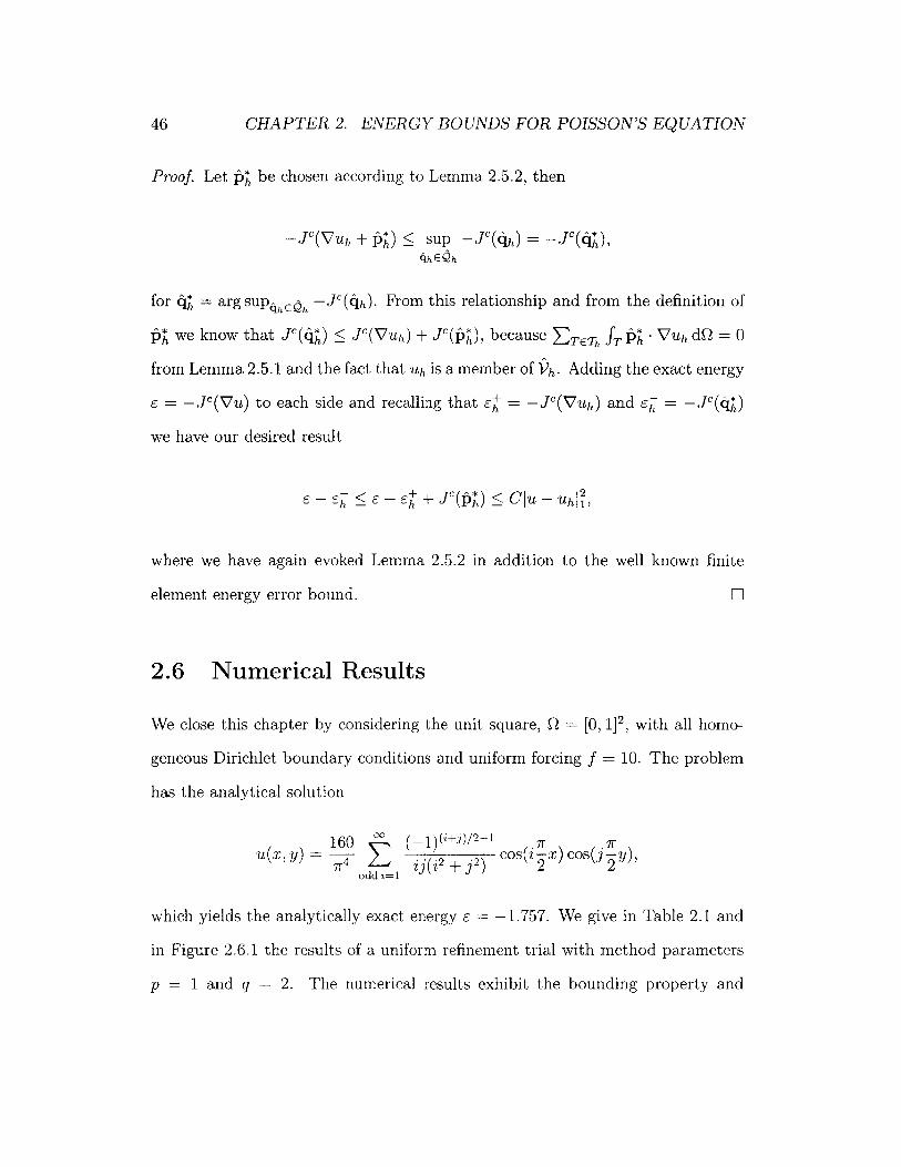
Proof. Let f* be chosen according to Lemma 2.5.2, then
- JC(Vuh + P*) sup - Jc(4h) = J'( )
$h6 Qh
for 4* = arg supghCgh Jc(4h). From this relationship and from the definition of
-we know that JC(*) Jc(Vuh) + Jc(p*), because ZTETh fT n*P VuhdQ = 0
from Lemma 2.5.1 and the fact that Uh is a member of 9h. Adding the exact energy
6 = -JC(Vu) to each side and recalling that e = -Jc(Vuh) and 6- = -Jc(4*)
we have our desired result
- - eh + Jc(f*) Clu - Uh1,
where we have again evoked Lemma 2.5.2 in addition to the well known finite
element energy error bound. E
2.6 Numerical Results
We close this chapter by considering the unit square, Q = [0,1]2, with all homo-
geneous Dirichlet boundary conditions and uniform forcing f = 10. The problem
has the analytical solution
160 (-1)(i+j)/2-1 co 7x
U(X, Y) = (i 2+ cos(2 ) cos(3 2 y),
odd i=1
which yields the analytically exact energy E = -1.757. We give in Table 2.1 and
in Figure 2.6.1 the results of a uniform refinement trial with method parameters
p = 1 and q = 2. The numerical results exhibit the bounding property and
46

2.6. NUMERICAL RESULTS
asymptotically approach the optimal convergence rate of 2, corroborating the
theoretical results developed in this chapter.
h (e - c)/e (E+ - _)/ _
1 0.7982 0.5554 1.7021 0.2678 0.1802 1.67
0.0738 0.0489 1.660.0190 0.0125 1.66
Table 2.1: Uniformly forced square domain.
-0.5 -
-1 -
-1.5 -
-2 -
-2.5 -
-3 -
I | | | |0 0.1 0.2 0.3 0.4 0.5
Mesh Diameter, h
Figure 2.6.1: Uniformly forced square domain convergence history.
o FE Approximation, Eh
V Lower Bound, ehA Upper Bound, -
El Bound Average, 6h
47

Chapter 3
Output Bounds For Poisson's
Equation
In this chapter, we will continue to keep the presentation simple by considering
only simple linear functional interior outputs of Poisson's equation. In particular,
we will develop upper and lower bounds, s*, on the output quantity
s - ffOu dQ, (3.0.1)
where u is the exact solution of Poisson's equation (2.0.1) and f 0 IT is a member of
Pr(T) for all elements T in Th. We stress, however, that more interesting outputs,
such as boundary fluxes, can also be treated using techniques previously employed
in the context of two-level methods (see, for example, the treatment of the normal
force output for linear elasticity in [PPP97] or the normal derivative output used
in the numerical examples of the next chapter).
48

3.1. WEAK CONTINUITY REFORMULATION
3.1 Weak Continuity Reformulation
To begin, we must formulate a generalized analogue to the minimization state-
ment (2.2.2). There are two parts to this task. First, we must replace the intrinsic
energy of the variational problem with an energy reformulation of the linear out-
put functional. Second, now that the minimization of the objective functional
no longer corresponds to the solution of our original equation, we must explic-
itly ensure that the minimizer is the solution to our problem by including it as
a constraint. Furthermore, to obtain both upper and lower bounds, we consider
two cases which vary by the sign of the original output. The resulting pair of
constrained minimization statements for the homogeneous' Dirichlet boundary
problem under consideration are
~Fs = inf - f Gi dQ + - VG+ . V(t* - i) dQ - f (Gi - U) dAT-*±Ev Jo 2 Qaj
s.t. VG - V d = Lfo dQ, V0 E V,
0-oTzbA dF = 0, VA E A,TCTh DT
(3.1.1)
where ii is any element of space V, and r, is a positive real scaling parameter which
serves both as a coefficient providing dimensional consistency in the engineering
context and as an additional degree of freedom which we will use to tighten the
bounds. The quadratic objective functional has been constructed so that all terms
but the desired output functional vanish when tb* is the exact solution, u, while
'The extension to non-homogeneous Dirichlet boundaries requires choosing u from the setof admissible functions and weakly enforcing the Dirichlet boundary data, UD, by replacing thecontinuity constraint with EZT faT oTd±A dF = E aI fy ~Tam A UD dF, VA 6 A.
49

CHAPTER 3. OUTPUT BOUNDS FOR POISSON'S EQUATION
the constraints enforce equilibrium and interelement continuity.
Paraschivoiu, Peraire and Patera [PPP97, PP98] originally proposed this re-
formulation in the context of two-level output bounding methods which appeal to
a second refined but localized finite element approximation and therefore provided
bounds only against a refined finite element approximation instead of the exact
infinite-dimensional solution. With this constrained minimization reformulation,
we can proceed more or less mechanically to apply the ideas from the energy
bound to this more general context. The development of the output bound is
very close to that for the energy bound, but with the extra burden of carrying
an additional Lagrange multiplier for the equilibrium constraint and of managing
the concurrent development of both upper and lower bounds on the output, as
neither arise implicitly from the finite element discretization.
3.2 Localization by Continuity Relaxation
Considering the Lagrangian of problem (3.1.1),
-F f i dQ + { V&+ . ( -ii) d - f ( - ii) dQ (3.2.1)
+ fo± dQ - V±. V ± dQ - at*J A* d',a n 7 T
50

3.2. LOCALIZATION BY CONTINUITY RELAXATION
we know, as we did for the energy bound, from the saddle point property of
Lagrange multipliers and from the strong duality of convex minimizations that
inf E(z;/AAI) < sup inf L*(&iA; @*, A*) = Ts.
AeA
for all (i/, A*) E V x A. The lower bounding minimization for a given I+ and
?/ is separable and, for an appropriate choice for li, provides non-trivial upper
and lower bounds on the exact output s.
3.2.1 Lagrange Multiplier Approximation
We proceed, as we did for the energy bound, to obtain approximate Lagrange
multipliers with a finite element discretization of the gradient condition of Equa-
tion (3.2.1). Let $1 = tVa, A± = 'A' t A0, and i = Uh, all of which we find by
solving the following discrete problems
1. Find nh E Vh such that
j VUh Vo dQ = fv dQ, Vv E Vh, (3.2.2)
2. Find <Oh E Vh such that
j Vv - V~h dQ = - f 0 v dQ, Vv E Vh, (3.2.3)
51
CHAPTER 3. OUTPUT BOUNDS FOR POISSON'S EQUATION
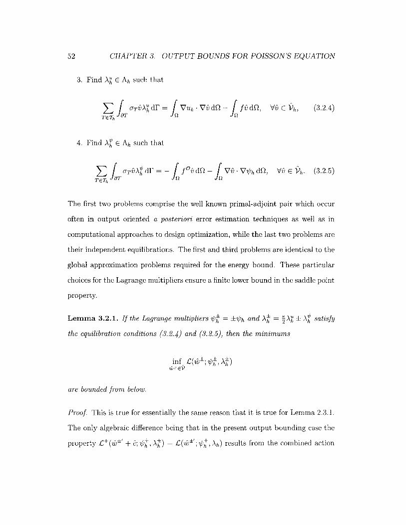
3. Find A' E Ah such that
-TJVdF = U -V dQ - f dQ, V E ), (3.2.4)
4. Find A E Ah such that
TJT d - f d-jVoW - VhdQ, Vi) E fh. (3.2.5)
The first two problems comprise the well known primal-adjoint pair which occur
often in output oriented a posteriori error estimation techniques as well as in
computational approaches to design optimization, while the last two problems are
their independent equilibrations. The first and third problems are identical to the
global approximation problems required for the energy bound. These particular
choices for the Lagrange multipliers ensure a finite lower bound in the saddle point
property.
Lemma 3.2.1. If the Lagrange multipliers $ = ±h and A' = ± A0 satisfy
the equilibration conditions (3.2.4) and (3.2.5), then the minimums
inf C(7b'; pg,- A-')
are bounded from below.
Proof. This is true for essentially the same reason that it is true for Lemma 2.3.1.
The only algebraic difference being that in the present output bounding case the
property E±(7i9' + ; 0±, A') = L(6bi'; 04, Ah) results from the combined action
52

3.3. LOCAL DUAL SUBPROBLEM
of both equilibration conditions.
3.3 Local Dual Subproblem
Restricting our attention to a single elemental subproblem, T E T , we first re-
write our local Lagrangian functional in a form suitable for applying the ideas
developed for the energy bound. Every term other than the dissipative energy
term, ! fr Vw - Vw dQ, must not involve derivatives of zib, which we can do
in the present case by application of the Green's identity - fT Vu - Vw dQ =
fT Au w dQ - far Vu - n w dF to obtain the equivalent local Lagrangian functional
L£(wl; te, " iI) = j Vw1 -Vwl dQ
(f - An) w± dQ + f -(UT-u + V n) w± dF + fa dQ2 T r
-F{j (fo - A ) widQ + (-A+V-n)w*dF±+ fedQ}. (3.3.1)
The functional we wish to minimize over w+ can now be defined as
JT (w±) , j Vwi -Vwl dQ - f w+ dQ - jg±w+ d', (3.3.2)
for f* = K{f - Aa} i± {f - AN} and g* {rT"uV -n}i{o-riA +
V' - n}. Thus, the local relaxed primal minimization once again corresponds
to a Poisson problem of the type represented in equation (2.0.1) with Neumann
boundary conditions posed on a single element.
As was the case for the energy bound, we do not require, and in general cannot
53

CHAPTER 3. OUTPUT BOUNDS FOR POISSON'S EQUATION
compute, the exact minimum of this local infinite-dimensional primal subproblem,
but we can apply the same technique of dualizing this minimization problem in
order to procure a computable lower bounding approximate to it.
Proposition 3.3.1. If we define the positive functional
J (q) ' q - q dQ, (3.3.3)
where q E H(div; T), then we have
J±(wi) ; -- J (q±), Vw± E 7-(T), Vq E Q±(T), (3.3.4)
for the set of functions
Q(T) -{q E -(div; T) V -qvdQ - j q -nvdF
=- f±v dQ - g v dr, Vv 'H'(T)}JT J'T
(3.3.5)
Proof. The local dual problem is derived as it was for the energy bound, but with
modified data and the addition of the scaling parameter, K. After expanding the
positive expression for q E Q'(T)
(q± - kVw) 2 dQ > 0, (3.3.6)
applying a Green's formula, and substituting the constraint from Q*(T), we ob-
54

3.3. LOCAL DUAL SUBPROBLEM
tain the expression
q -q d+ jVw' -Vw dQ -- f+'wd* dg - 0g w-' ;> 0. (3.3.7)
Identifying J#(wi) and J (q*) we arrive at the desired expression for the local
lower bound. l
As the functional J1(wi) only contains the terms from the Lagrangian that
depended on w*, we must reintroduce the constant terms to secure the complete
contributions from the local dual subproblems
S f (r ± @h) dQ + sup -- JS(q'). (3.3.8)T q±EQ±(T)
3.3.1 Subproblem Computation
Consider the splitting implied by the definition qh = rVu+ q±q0. Propagation
of this definition into the elemental subproblem reveals through the linearity of
the gradient condition that indeed qu and q1P can be computed independently.
The resulting subproblems are
qu =arg inf JC(qh),
qh =arg inf Jc(qh),qh E Q" (T)
55
CHAPTER 3. OUTPUT BOUNDS FOR POISSON'S EQUATION
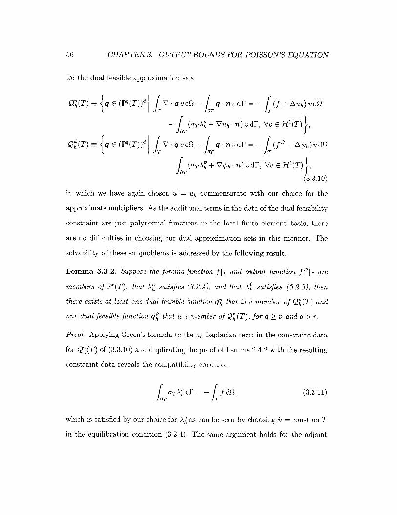
for the dual feasible approximation sets
Qh(T) q E (Pq(T))d jV.qvdQ- q-nvdd= - (f + Uh) v dQTT J T7J1T
- I(uT Au - VUh - n) o d1F, Vv E H (T),
Q(T) q E (pq(T))d V qvdQ - q - nvdF = (f O - Ah) v dQTT c1T }T
f(o-T A -+- V~bh - n) v dr, Vv Ez 'H(T),
(3.3.10)
in which we have again chosen ii u=, commensurate with our choice for the
approximate multipliers. As the additional terms in the data of the dual feasibility
constraint are just polynomial functions in the local finite element basis, there
are no difficulties in choosing our dual approximation sets in this manner. The
solvability of these subproblems is addressed by the following result.
Lemma 3.3.2. Suppose the forcing function f IT and output function f 0 IT are
members of Pr(T), that Au satisfies (3.2.4), and that A0 satisfies (3.2.5), then
there exists at least one dual feasible function qu that is a member of Qu(T) and
one dual feasible function qV that is a member of QO(T), for q > p and q > r.
Proof. Applying Green's formula to the uh Laplacian term in the constraint data
for Qu(T) of (3.3.10) and duplicating the proof of Lemma 2.4.2 with the resulting
constraint data reveals the compatibility condition
JT TAu dF = - f dQ, (3.3.11)aT h J T
which is satisfied by our choice for Au as can be seen by choosing () = const on T
in the equilibration condition (3.2.4). The same argument holds for the adjoint
56

3.4. OUTPUT BOUND PROCEDURE
dual subproblem, yielding the analogous compatibility condition
/ITUTA dF = -jfo dQ,h~ fT
(3.3.12)
for f0 and Ab.
With the subproblem splitting just defined, the aggregated contributions to
the upper and lower bounds become
f ('Ui h±) dQ ± Jc(KVUh + - efu± hK 2 h
f (nU i Oh) dQ Vuh. Vuh dQ +
+ 1 4u -4) dQ
=- fh dQ +j
K 1t ~JC(q%) ± J"(4f)
44
in which we have invoked (3.2.2) with V = Uh as well as used orthogonality rela-
tionships analogous to that proved in Lemma 2.5.1.
3.4 Output Bound Procedure
The introduction of the scaling parameter r allows us to optimize the sharpness of
the computed bounds in addition to providing dimensional consistency. From the
previous section we have the expression for the upper and lower output bounds
S± =-hIKU ZSh 8 hK h 7
s = ~
= J0 -VuhdQ
I jc(4(),K h
57
( 24u i 4 h)

58 CHAPTER 3. OUTPUT BOUNDS FOR POISSON'S EQUATION
where
h 4u A4dQ- f~h dQ, zu =Jc (4), zb =Jc(4"), (3.4.1)
Maximizing the lower bound and minimizing the upper bound with respect to K
yields the optimal value n2 = zO/z.
The complete method with optimal scaling for upper and lower bounds on
linear functional outputs can now be written as three steps:
1. Global Approximation:
Find UhE Vh such that
VUh - VvodQ = jfvdQ, Vv E Vh, (3.4.2)
and find 4h E Vh such that
jo VV- V~h dQ = - f 0 v dQ, Vv E Vh. (3.4.3)
2. Global Equilibration:
Find Au E Ah such that
T j uh -*VdQ - f dQ, V E Vh, (3.4.4)TTh7 J8T f9 d o
and find A' E Ah such that
o-TiAJ d = - f dQ - W - VPhdQ, V c 9h. (3.4.5)T ETh J T JQ I

3.4. OUTPUT BOUND PROCEDURE
3. Local Dual Subproblems:
Find 4u such that
4uh= arg inf JC(4), (3.4.6)4heQuh
find di such that
= arg inf J"(4h), (3.4.7)
and, from equation (3.4.1) and the optimal K, calculate
sh Sh± 2 ZuZh. (3.4.8)
The local dual subproblems for the output bounds can be solved in the same
manner as the local energy dual subproblems. The important point being that
once the finite element approximations Uh and 4 have been computed, the solu-
tions can be equilibrated and quantitative bounds computed on the exact output
to the infinite-dimensional continuum equation with asymptotically linear cost in
the size of the finite element discretization and in parallel.
3.4.1 Properties of the Output Bounds
The upper and lower bounding properties are direct consequences of the saddle
point property of the relaxed constrained minimization reformulation (3.1.1) and
the local dual property of Proposition 3.3.1. The following proposition addresses
the accuracy of the computed bounds by showing that the bounds will converge at
the optimal rate when both the primal and adjoint finite element approximations
are in the asymptotic convergence regime.
59

CHAPTER 3. OUTPUT BOUNDS FOR POISSON'S EQUATION
Proposition 3.4.1. Suppose that uh, Oh, A, and A' are solutions of the above
finite element approximation problems and equilibration problems, then
S - ClU -Uh|1|@ - $hI1,
(3.4.9)s+i - C u h|1|@ -@Ohl1-
Proof. Applying the definitions from the procedure, we know that the lower a
posteriori bound, for instance, itself has the bound
s- < s - s- 2VZhZh.
The arguments of Lemma 2.5.2 can be applied to the zu and z factors to show
that they are bounded by Clu - uhl1 and Cj#b - Ohl1, respectively. 1
3.4.2 Computational Complexity
The first step of the procedure solves two standard finite element problems. The
finite element solver has an asymptotic complexity of O(Nk), where N is the
number of unknowns in the discretization and 1 < k < 3 is a property of the
solver. A fully dense direct solver would provide the worst case complexity of
k = 3. Any solution method must visit each unknown at least once, in order to
assign the solution, thus the best case complexity is k = 1. Using Ladeveze's
method and assuming that the number of elements sharing a vertex is bounded
from above, the second step can be performed by solving V small local patch
subproblems, where V is the number of vertices in the triangulation. This yields
an asymptotic complexity of O(V) for the equilibration step. Finally, solving a
60

3.4. OUTPUT BOUND PROCEDURE
sequence of small local elemental subproblems results in an asymptotic complexity
of O(K). As we have assumed that the number of elements sharing a vertex is
bounded from above, the asymptotic complexity of the latter two steps of the
procedure can be stated as O(V). We deduce that the leading order asymptotic
complexity of the entire procedure is O(Nk) since V < N and k > 1. The
important point being that the output bound computation does not increase the
asymptotic cost of the approximation. Moreover, the output bound computation
delivers certainty, which cannot be obtained by merely increasing N.
More relevant than the number of unknowns an approximation requires, how-
ever, is the desired precision of the approximation. Assuming that the finite
element approximation achieves 0(hP) convergence in the 'Hl-norm measure of
the error for both the solution and the adjoint, Proposition 3.4.1 informs us that
the bound gap will have 0(h 2 P) asymptotic convergence. For a desired precision,
Atoi, we have Atoi - h2'P. Therefore the required element diameter, h, for a given
precision will be O(A$). Finally, uniform refinement yields N ~ and thus the
asymptotic computational complexity of the complete procedure to produce an
output approximation of a prescribed accuracy is 0 A( dk). The important con-
clusion from this analysis is that the method can compute approximate outputs of
prescribed precision in polynomial time. For example, a problem posed on a two-
dimensional domain and approximated with a linear finite element approximation
has an asymptotic computational complexity of O(A-j).
61

CHAPTER 3. OUTPUT BOUNDS FOR POISSON'S EQUATION
3.5 Adaptive Refinement
The elemental subproblems provide local error information which can be used as
an indicator for mesh adaptivity via the elemental contribution to the bound gap,
Ar = LJy(qu) + -!J4(q'). The elemental bound gaps can serve as informative
mesh adaptivity indicators for controlling the error in the output, as was done
in [PP97] for a two-level error bound method. Adaptive indicators have long been
the principle business of error estimators. For example, see [Ver94, ODRW89] for
energy-norm error measures, and more recently [BR96a, BKROO, RS97, SBD+00]
for more general measures. The principle business of the method we have pre-
sented, however, is to certify the precision of an approximate output. Nevertheless,
the local bound gap contribution can be used to improve both the precision of the
output and the sharpness of the certificate using adaptive refinement.
It is well known that the error in a finite element solution contains a local
contribution as well as a global contribution called the pollution error which both
need to be taken into account for effective adaptive refinement [BSUG95b, Ain99].
In addition, sophisticated adaptive algorithms attempt to predict the optimal
element diameter in order to both reduce the number of adaptive steps required
and the number of elements contained in the final mesh. We do not attempt to do
either of these things, but instead provide a simple demonstration of the potential
for the local bound gap contributions to act as refinement indicators.
At each level of refinement, only elements for which AT > Atoi/K are refined,
where At01 is a user specified tolerance for the precision of the output from the
global approximation and K is the number of elements in the triangulation at that
level. The meshes are generated and adaptively refined using the freely available
62

3.6. NUMERICAL RESULTS
Triangle mesh generator [She96]. By preferentially refining the mesh elements
contributing more than a target average error contribution, we obtain a simple
but effective adaptive strategy.
3.6 Numerical Results
We verify the method numerically for three cases: constant forcing on the unit
square, linear forcing on the unit square, and zero forcing on an L-shaped domain
with a corner singularity. Linear finite elements, p = 1, and quadratic subprob-
lems, q = 2, are employed with the domain average output
s= fOu dQ,
where f 0 = const, for all cases.
All three cases have analytically exact solutions with which we are able to
verify the method and calculate the effectivities of the bounds,
* = , (3.6.1)
which indicate the sharpness by comparing the error in the bounds to the error
in the finite element approximation. The results are summarized in Table 3.1.
63

CHAPTER 3. OUTPUT BOUNDS FOR POISSON'S EQUATION
Uniformly Forced Square Linearly Forced Square Corner Singularityh s- s+ 0-0 s- s+ 0- 0+ s- s+ 0- 0;1 0.156 0.632 1.0 1.4 0.860 1.276 5.1 2.9 0.702 0.897 5.1 6.0
0.288 0.446 1.0 1.5 1.050 1.171 5.7 3.5 0.761 0.829 4.3 5.10.334 0.377 1.0 1.5 1.106 1.137 5.9 3.8 0.781 0.805 3.6 4.4
- 0.347 0.358 1.0 1.5 1.120 1.128 6.0 3.8 0.788 0.797 3.1 3.9
Table 3.1: Output bounds and effectivities for three numerical test cases.
3.6.1 Uniformly Forced Square Domain
The first case is a uniformly forced unit square domain with f = 0 = v10. The
analytical solution is given by
16/E (-1) (i+.0/2-1U(z, y) = 4 cos(z z) Cos(j-)
odd i=1 I) 2
This case is special in that the forcing and output are identical and the boundary
data is homogeneous, leading to primal and adjoint problem data which differ
by only a sign. It is well known that for this special case, called compliance,
the finite element approximation for the output is a lower bound. The numerical
results demonstrate that our method, while more expensive, does no worse than
the inherent bound for this special case. The results for both the finite element
approximation and the output bounds asymptotically approach the optimal finite
element convergence rate of O(h 2 ). This example also evinces that the bound
average, Sh, can sometimes be a more accurate output approximation than the
that from the finite element approximation.
The uniformly forced Poisson equation posed on a two-dimensional domain
models the cross-sectional velocity distribution for viscous duct flow. Figure 3.6.2
illustrates how the method might be used to study the dependency of an output
64

3.6. NUMERICAL RESULTS
0.6-
0.5-
0.4-
0.3-
0.2 -
017A
O
0
FE Approximation, Sh
Lower Bound, sh
Upper Bound, shBound Average, sh
I I I I |0.1 0.2 0.3 0.4 0.5
Mesh Diameter, h
Figure 3.6.1: Uniformly forced square domain convergence history.
on a parameter. In the context of duct flow, the uniform output we have been
considering calculates the flow rate. The upper and lower bounds our indicated
by horizontal bars, the bound average by a black box, the finite element approxi-
mation by a hollow circle and the analytically exact solution by a grey line.
3.6.2 Linearly Forced Square Domain
The second case is a linearly forced square domain with f0 = 1, and the forcing
and non-homogeneous boundary conditions chosen to produce the exact solution
u(x, y) = 3 y2(1 - y) + 4xy.
65

CHAPTER 3. OUTPUT BOUNDS FOR POISSON'S EQUATION
4-
3-
C
1-
00.8 1 1.2
Figure 3.6.2: Theheight.
dependency of flow rate through a viscous duct on channel
As this test case is not a special case, the convergence histories of Figure 3.6.3
depict the more general situation in which none of the computed quantities coin-
cide. Whereas in the first example we saw that the bound average can possibly be
a more accurate output approximation than the finite element approximation, in
this example we see that this is definitely not always true since the finite element
approximation for the output is 0.5% better. As for the first example, the results
for both the finite element approximation and the output bounds asymptotically
approach the optimal finite element convergence rate of 0(h2).
T
I 1 10.2 0.4 0.6
Channel Height0
66

3.6. NUMERICAL RESULTS 67
o FE Approximation, shp Lower Bound, sh
1.3 _ A Upper Bound, stl Bound Average, sh
1.2-
-., 1.1-
1-
0.9-
I I |0 0.1 0.2 0.3 0.4 0.5
Mesh Diameter, h
Figure 3.6.3: Linearly forced square domain convergence history.
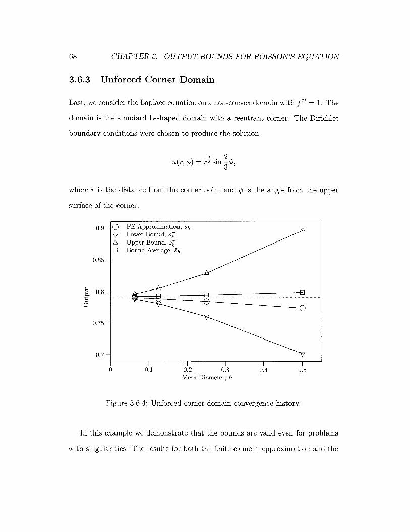
CHAPTER 3. OUTPUT BOUNDS FOR POISSON'S EQUATION
3.6.3 Unforced Corner Domain
Last, we consider the Laplace equation on a non-convex domain with f0 = 1. The
domain is the standard L-shaped domain with a reentrant corner. The Dirichlet
boundary conditions were chosen to produce the solution
22u(r,#) = rsin -'3,
where r is the distance from the corner point and # is the angle from the upper
surface of the corner.
0.9-
0.85 -
0.8-
0
0.75 -
0.7-
0I I I I I
0.1 0.2 0.3 0.4 0.5Mesh Diameter, h
Figure 3.6.4: Unforced corner domain convergence history.
In this example we demonstrate that the bounds are valid even for problems
with singularities. The results for both the finite element approximation and the
FE Approximation, shLower Bound, s-Upper Bound, shBound Average, sh
68
017Z\1:1

3.6. NUMERICAL RESULTS 69
output bounds asymptotically approach the optimal finite element convergence
rate of 0(h) for elliptic problems posed on a domain with right-angled reentrant
corner [SF73]. Once again we see that the bound average has the potential to be
a better output approximation than the finite element method.
Finally, Figure 3.6.5 displays the end results of the simple adaptive strategy
previously outlined applied to the unforced corner domain problem.

OUTPUT BOUNDS FOR POISSON'S EQUATION
u: -0.35 -0.05 0.25 0.55
(a) Adaptive solution field.
W: -3.5x10⁻² -2.Ox1O-2 -5.Oxl03
(b) Adaptive adjoint field.
Gap: 0.02 0.04 0.06 0.08 0.1 0.12 0.14 0.16 0.18
(c) Elemental bound gap contri-butions on intermediate mesh.
(d) Final adaptive mesh.
Figure 3.6.5: Unforced corner domain adaptive solutions, local indicators andmeshes.
CH APT ER 3.70

Chapter 4
Output Bounds for the
Advection-Diffusion-Reaction
Equation
We will consider the steady scalar diffusion-dominated advection-diffusion-reaction
equation posed on a polygonal domain Q in d spatial dimensions with boundary F
composed of complementary regions ID and FN. The problem is written in weak
form as: find u c U such that
a(u, v) = E(v), Vv E V,
with the coercive non-symmetric bilinear form defined as
a(w, v) = vVw -VV + pwv + (a -Vw) v dQ,
(4.0.1)
(4.0.2)
71

CHAPTER 4. OUTPUT BOUNDS FOR THE ADR EQUATION
for a strictly positive real coefficient v E Ec' (Q), a nonnegative real coefficient
t E L(Q), and a prescribed vector field a E H(div; Q) which is assumed for sim-
plicity to be incompressible, V-a = 0. The set of admissible functions is defined as
U (Q) = {v E VK(Q) | vlrD = UD }, with Dirichlet boundary data UD E 2(FD)
and the space of test functions is defined as V(Q) { {v E V((Q) I VjrD = 0 }.
Additionally, we require the prescription of the solution field on inflow bound-
aries, that is F- c FD C F for - = (x E F | a - n(x) < 0}. The linear forcing
functional
e(v) = fdQ + gv dF, (4.0.3)
includes both interior f E - 1 (Q) and Neumann boundary g E R- -(FN) contri-
butions.
We are not directly interested in the field solution u, however, but in bounded
linear functional outputs from it, s = e 0 (u). In particular, we will develop upper
and lower bounds on the outputs produced by linear functionals such as
E = -- f 0 w dQ + j g w dF, (4.0.4)
for f 0 E 7-'(Q 0 ) and go E - (F9).
In order to guarantee bounds for any level of refinement, the method presented
in this chapter requires that the coefficients v, y, and a, and forcing data f, f0 ,
g and go are all piecewise polynomial. In addition, we will consider only constant
coefficients v and t for simplicity.
72

4.1. CONSTRAINED MINIMIZATION REFORMULATION
4.1 Constrained Minimization Reformulation
In the context of the Poisson problem, we reformulated the model problem as a
constrained minimization with weakly enforced continuity in order to localize the
bounds computations and to obtain bounds on more informative output quantities
than the abstract energy. In the present context of a non-symmetric operator, the
reformulation also provides the means by which we can treat problems without
an intrinsic minimization principle.
4.1.1 Weak Continuity
As before, we begin by introducing a triangulation of the domain, 7h, into non-
overlapping open subdomains, T, called elements, for which UT h T = (. We
denote by DT the edges constituting the boundary of a single element T, and by
9Th the network of all edges in the mesh. On this triangulation, we introduce the
broken space
9=E {v E L2 IvITE '(T), VTE h}. (4.1.1)
in which the continuity of 9 is broken across the mesh edges, 89Th. Note that
the broken space relaxes the Dirichlet boundaries in addition to the interelement
continuity so that we have V C 9 and U C 9.
We enforce continuity between the elemental subdomains weakly through the
bilinear form b : V x A -+ R
b(zb, A) = O o-rA dl',T T
73

CHAPTER 4. OUTPUT BOUNDS FOR THE ADR EQUATION
where, for TN E Th and an arbitrary ordering of the elements, T < TN,
-T(X) { xETTN,T< TN (4.1.2)
+1 otherwise
is a constant on each edge, and the edge functions A are members of the dual trace
space A =H17T,'H-2 (BT).
In addition to weak enforcement of interelement continuity, the Dirichlet data
will also be enforced weakly in our reformulation through the forcing provided by
the linear functional D : A --+ R
ED(A)= J 0-TUDA dl?, (4.1.3)
so that b(b, A) = ED(A) for all 'i E U and A C A.
4.1.2 Operator Decomposition
A non-symmetric operator can be split into symmetric, as(w, v) = as(v, w), and
antisymmetric, ass(w, v) = -ass(v, w), contributions
1 1as(w, v) = [a(w, v) + a*(v, w)] , ass(w, v) =- [a(w, v) - a*(v, w)] , (4.1.4)
2 2
where a*(v, w) is the formal adjoint of a(w, v) for w E U and v E V. Integration
by parts yields a(u, w) = a*(w, u) + C*, from which we note that ass(w, w) = 1C*
and thus a(w, w) = as(w, w) + 1C*. Additionally, we note from the above that
a(v, w) = as(v, w) + ass(v, w) = as(w, v) - ass(w, v). It is easily shown for the
T4

754.1. CONSTRAINED MINIMIZATION REFORMULATION
advection-diffusion-reaction equation that
a*(v,w) = I
C* = fD
vVv -Vw + tvw - (a -Vv)w dQ +IFN
v (a - n) wdF,(4.1.5)
(a -n)U2 dF,
and therefore
vVw -Vv + pwvdQ +
Vw) v dQ - -12 rN
- w (a -n2 frN
w (a -n) o dH.
4.1.3 Constrained Minimization Statement
Using the above definitions we can write the following energy-like functional E
S--+ R
=a'(b, iv) + I C* - f(b) + f(ii) - a(z, ii),2(4.1.7)
where ii is a member of U. This functional has two essential properties. First, it is
coercive on the space 9 for y > 0 and for p = 0 is coercive on the quotient space
9 \ NO, where NPO is the space of constants over each element. Second, it reduces
to zero when & = u.
The weakly continuous constrained minimization problem for the non-symmetric
model problem can now be written as
:s = inf
s.t. a(*, ) = f W)
b(i, A) = ED(A),
(4.1.8)V' E V,
VA E A,
: to (Z+) + "E( )
a(w,v) =
ass(w, v) = j (a
)v dF,(4.1.6)

CHAPTER 4. OUTPUT BOUNDS FOR THE ADR EQUATION
where rK is a strictly positive real scaling parameter which provides dimensional
consistency as well as an additionally degree of freedom which we will later use
to tighten the bounds. This apparently trivial constrained minimization reformu-
lation, first introduced in [PP98, PPP97] and whose constraints also arise in the
context hybrid finite element methods [BF91], serves as the launching point for
developing our method.
4.1.4 Localization by Lagrangian Relaxation
The above constrained minimization (4.1.8) has the Lagrangian: L* : x V x A -
R
+ as wi ) + C* -f (zb) + f(u) - (G±, f) (4.1.9)
+ f(V$') -a(Th., ip) + fD(A)- b(7b' A:)
for given candidate Lagrange multipliers /* C V and A* E A. The Lagrangian
saddle point property for the constrained minimization reformulation engenders
the following relationships for all ( 1*, A*) E V x A
inf L'(tb±; 4 <, ) < sup inf. L*(ib*; 0±, A') = -s, (4.1.10)
A+ EA
which we will exploit for developing inexpensive local subproblems for computing
bounds. Equality on the right of (4.1.10) results from the strong duality of convex
minimizations, but the bound property would still hold with weak duality.
76

4.1. CONSTRAINED MINIMIZATION REFORMULATION
4.1.4.1 Lagrange Multiplier Approximation
We compute approximate Lagrange multipliers using the finite element method
by first choosing ,I =4th, ~* = ± A", and i = Uh, where Uh and 4h are
members of the usual piecewise polynomial finite element approximation set
Uh-= {w E I Tf|r E PP(T), VT E Th },
and space
Vh { v E V I VIT E PP(T), VT E T },
and both Au and A0 are members of the piecewise polynomial space
Ah = { A E A | Al, E PP(7), V7y E OT}
. We have used the notation PP(T) for the space of polynomials on element T (in
d spatial dimensions) with degree less than or equal to p, and PP(-) for the space
of polynomials on edges 7 (in d - 1 spatial dimensions) with degree less than or
equal to p.
By approximating u, the optimizer of the constrained minimization (4.1.8),
with Uh and noting from (4.1.4) that a(v, Uh) = as(Uh, v) - ass(uh, v), we can write
an approximate gradient condition
- {-f(0) + a(i, Uh) + b(b, A')}2 {
77

CHAPTER 4. OUTPUT BOUNDS FOR THE ADR EQUATION
with 9h - { E E 2 | VIT c PP(T), VT E T }. We can compute approximate La-
grange multipliers from (4.1.11) by solving the discrete problems:
Find Uh E Uh such that
a(uh, v) = e(v), VV E Vh, (4.1.12)
Find $h E Vh such that
a(v, #h) = -i(v), VV E Vh, (4.1.13)
Find Au E Ah such that
b(i, Au) = E(i) - a(Uh, W), Vi E h, (4.1.14)
Find A0 E Ah such that
b(i, AO) = -E'() - a(i, $h), V'b E Vh. (4.1.15)
The first two problems are standard finite element approximation problems and
the second two problems are equilibration problems which can be solved with an
asymptotic complexity that is linear in the number of vertices in the triangulation
using Ladeveze's procedure [LL83].
Lemma 4.1.1. If the Lagrange multipliers Au and A) satisfy the equilibration
78

4.2. ELEMENTAL SUBPROBLEMS
conditions (4.1.14) and (4.1.15), then the minimizations
inf L*(z; -, ± \u t A)) (4.1.16)
are bounded from below.
Proof. A strictly positive reaction term in as(tb*, &:+) ensures that the lower
bounding minimization (4.1.10) is bounded below without the aid of equilibra-
tion. For p = 0, the constant function is not controlled by as(zb*, 1i+) and with-
out equilibration it would become possible for the subproblems, which only have
Neumann boundary conditions, to be driven to arbitrarily large negative values of
the Lagrangian functional. Equilibration ensures the nullification of the constant
function, as can be checked by setting ' = const in (4.1.14) and (4.1.15). El
4.2 Elemental Subproblems
The continuity relaxation of §4.1.4 decomposes the triangulation so that after
computing the approximate Lagrange multipliers we may consider each element
independently when computing the bounds. We perform the global lower bounding
minimization (4.1.10) by minimizing the local contribution of the Lagrangian on
each elemental subdomain and accumulating the results to produce upper and
lower bounds on the exact output
s- < s < s+ (4.2.1)T ETh TETh
We can write the local contribution of the Lagrangian on an arbitrary element
79

OUTPUT BOUNDS FOR THE ADR EQUATION
T of the triangulation T as
s= inf -as(w+, *) + l(w+) + C, (4.2.2)w±E7-H2(T) 2 ( ±(± T
where we have collected the constant and linear contributions to the local La-
grangian with the definitions
if (v) = { - E(V) - aT(v, Uh) ± bT(v, A) (4.2.3)
-±E (v) - aT(v,, V) -- bT(v,
{rT(h) - fD(Au) + C}
± {T(?I)
Ah,
(4.2.4)
+ D
The subscript T denotes restrictions to a single element of the triangulation. For
example, we have
aT(w, v) = T
T(V) = fvdQ+jJT JfrN
vVw - Vv + pwv + (a -Vw)v dQ,
gvdf,
in which rI denotes the local Neumann edges, BT n pN as well as
bT(w, A') = UTwA d1F,
S(A) = TUDA dFJr Dg
in which IF' denotes the local Dirichlet edges, B9T n IPD
CH APT ER 4.80
Ce =

4.2. ELEMENTAL SUBPROBLEMS
Recall from §4.1.2 that for the advection-diffusion-reaction equation we have
asr(w, w) = vIVw|2+ w2 d + - (a .n) w 2 dF, (4.2.5)T JT2 rN
which is coercive on V(T) for y > 0 (and on V(T) \ PO(T) for p = 0) for all T in
Th because c -n is perforce positive on FT.
4.2.1 Dualization of Local Minimization
The localized unconstrained minimization (4.2.2) remains uncomputable in gen-
eral, since the minimization must be performed over an infinite-dimensional space
in order to guarantee the bounding property. Nevertheless, by once again apply-
ing the powerful ideas of Lagrangian saddle point theory, we can compute a lower
bound to this lower bound and thus procure guaranteed computable bounds on
the exact output of interest.
Proposition 4.2.1. The optimal value of the local unconstrained minimization
problem (4.2.2) can be found by solving the local constrained maximization problem
-s= sup - a u * * * ,*)) + C±
,1(,C2 (T) (4.2.6)q±E(l22(T))
s.t. rc "((q+,r±),v) = -E(v), Vv E 7-(T),
where the form a" d: (L2(T))d x W'(T) x (L2(T))d x 7-(T) -+ R is defined as
a u((q, r), (p, v)) = vq -p + prv dQ + - j(a - n)rv dE. (4.2.7)T ~ 2 rN
81

OUTPUT BOUNDS FOR THE ADR EQUATION
and the form cT": (L2(T))d x H7(T) x H1(T) - R is defined as
cu((q, r), v) = vq - Vv + prv d + (a - n)rvd. (4
Proof. We begin formulating the dual problem by introducing the auxiliary vari-
able i- E (L2(T))d which satisfies the constraint
IT v(Vwl - Tri) -p d = 0, Vp E (L 2(T))d (4.2.9)
and the auxiliary variable p* E C2 (T) which satisfies the constraint
Vv E L2(T). (4.2.10)
Defining B to be the set of all triples (wi,7ripi) in 'H0(T) x (1 2(T)) x2
which satisfy the constraints (4.2.9) and (4.2.10), we can write the local uncon-
strained minimization (4.2.2) as an equivalent constrained minimization
inf(w±,r±,p*)E
'- { j v(irI)2 + p(pI)2 dQ +2 Jr
This equivalent constrained minimization can be formulated as the Lagrangian
saddle point problem
sup infk W 2'(T)
qrE(,C2 (T) )
P ±EZ 2 (T)
J± (w', 7r±, p±; q±, r±) + CT,
ITp (w+- p)v dQ + -J
2 frN(a - n)(wi - P*)v dF = 0,
-s± =2 I(a
frT
(4.2.11)
-FsT (4.2.12)
CH APTER 4.82
(4.2.8)
- n) (p±)2 dFA

4.2. ELEMENTAL SUBPROBLEMS
where the Lagrangian functional is defined as
J(w, 7r, p; q, r) = rfv( I7r+ - q)7r± + ( p )p± dQ
+ K j(a - n)( pi - r)p± dF
+ { j vVw- q' + puw r+ dQ (4.2.13)
+ - (a - n)wlr*dF2 rN
+ f(w).
Equality on the left of (4.2.12) results from the quadratic Lagrangian functional,
but the bound method can also be derived when only weak duality holds.
A necessary condition for optimality of the inner minimization of (4.2.12) with
respect to the principle primal variable w+ is
r, vVv - q±'* + pvr±'* dQ + (a - n)vrC* dF =-T(v), Vv E 'H'(T),
(4.2.14)
where the superscript * indicates optimality of the variable. Necessary conditions
for optimality with respect to the two auxiliary primal variables -r* and p* are
J v(7ri'* - q±'*)p dQ = 0, Vp C (L2(T))d, (4.2.15a)
p(p'* - r+'*)v dQ + r (a -n)(p+,* - r±'*)v dF = 0, Vv E E 2 (T).Jo 2 JrN
(4.2.15b)
After substituting the auxiliary variable optimality conditions (4.2.15) into the
83

CHAPTER 4. OUTPUT BOUNDS FOR THE ADR EQUATION
Lagrangian (4.2.13) and retaining the principle primal variable condition (4.2.14)
as a constraint in the outer maximization of the saddle problem (4.2.12), we arrive
at the local dual constrained maximization (4.2.6) formulation of the original
unconstrained local minimization (4.2.2). El
Significantly, we may inexpensively compute a quantitative lower bound on
T-s, and thereby upper and lower bounds on the exact output s, by performing
the local dual constrained maximization (4.2.6) over a finite-dimensional set so
long as the set is rich enough to allow the dual constraint to be satisfied exactly.
Indeed, while maximization will improve the sharpness of the bounds, we only
require dual feasibility to obtain bounds.
4.2.2 Dual Subproblems
The local dual maximization problem (4.2.6) has the optimality conditions: find
(qi, ) E (L2(T))d x 70(T) x 71(T) such that
-saiu ((q*,r), (p, v)) - ,cp"((pv), 7I) =0, V(p,v) E (L42(T) x 'H'(T
(4.2.16a)
- KcT"((q', r'), v) =tf'(v), Vv E H'(T), (4.2.16b)
which, as a result of the linear equality constraint and convex objective functional,
are both necessary and sufficient. For the purpose of computing bounds, the
Lagrange multiplier (* is an artifact of solving the constrained maximization
problem and we will not make direct use of it.
As formulated, the optimality conditions depend explicitly upon the scaling
84

4.2. ELEMENTAL SUBPROBLEMS
parameter K, but the substitutions
-q, -Uh-K
1 1 12 K 2
will transform the above -dependent problems into the following two K-independent
problems: find (qu, ru,(u) E (L2(T))d x 7H((T) x 7H1(T) such that
aT ((q", ru), (p, v)) + cT"((p, v), ) =0,
cTj"((qu, ru), v) =N'(v),
V(p,v) E (C 22(T))d x -1(T),
(4.2.17a)
Vv E H'(T) (4.2.17b)
and find (qv),,ro , ) E (L2(T))d x X11 (T) x 71(T) such that
dua ( , v), () =0,aT ((q r'), (p, V)) + 4U ((p , 0 V(p,v) E (12 (T)) d
v), Vv E 'H(T),&
x -H'(T),
(4.2.18a)
(4.2.18b)
where we have defined the the localized residual forms
(4.2.19)
(4.2.20)
Equilibration ensures that all dual feasible functions (qu, ru) and (q), r )) are
orthogonal to the local finite element basis.
Lemma 4.2.2. Any pair (qu,ru) in (L 2 (T))d x H1(T) that satisfies the con-
85
(qi, r*,' )= (VUh - q"2 K
R+(v) =T(V) - aT(Uh, v) - bT(v, Au),
N4(v) - Ef(v) - aT(v, Oh) - bT(v, A").
cp"((ql, r'), v) =Nf4(

OUTPUT BOUNDS FOR THE ADR EQUATION
straint (4.2.17b) has the orthogonality property
adu((qu, ru), (Vv, v)) = cu((qu, ru), v) = 0, Vv E Vh(T),
and any pair (q, r") in (L2(T ))d x H'(T) that satisfies the constraint (4.2.18b)
has the orthogonality property
aT"((q*,r*), (Vv,v)) = c"((q', r'), v) = 0, Vv E Vh(T).
Proof. This is a direct consequence of equilibration provided by (4.1.14) and (4.1.15),
and the definitions (4.2.19) and (4.2.20). E
With the above orthogonality property we can calculate the objective from
dual feasible functions (qu, ru) and (q*10, rO) using
- s = - {a "((q", ru), (qu, ru)) - CI
2 rI a {((q i, r ) , (q , r )))
t la "u((q" , r") , (qo , r11))
with the definitions
1C" =T (Uh) - asT(Uh, Uh) C(A) ± ,
C = ) ( )
CT)=eT(Vh) + f A)
(4.2.21)
(4.2.22)
+ CT} (4.2.23)
(4.2.24)
(4.2.25)
86 CHAPTER 4.

4.2. ELEMENTAL SUBPROBLEMS
4.2.3 Subproblem Computation
Recall from §4.2.1 that, by virtue of the dualization of the local minimization
problem, we can choose a finite-dimensional set within which to search for the
dual functions (qU, ru) and (q, rp), so long as the set is rich enough to admit at
least one pair (qU, ru) satisfying (4.2.17b) and at least one pair (qo, r*) satisfy-
ing (4.2.18b).
Lemma 4.2.3. If the interior data f IT, (a -Vuh)IT, f 0 IT, and (a V'Oh)IT are
all members of P"'(T), the boundary data g|,, g0 ,, and ((a - n)h)I-, are all
members of P"(y) for all -y E &T, and the continuity multipliers Au and A0 are
equilibrated according to (4.1.14) and (4.1.15), then there exists at least one pair
(q ,ru) e (pq(T ))d x IPq(T) satisfying (4.2.17b) and at least one pair (qV,rv) E
(p(T ))d x IPq(T) satisfying (4.2.18b) for q > p and q > m.
Proof. Let qu = q"D + q, with qu -n = -orTA- v(Vuh n) on BT \ F', q"Dn=
-o-TAu on F , qu -n = 0 on 0T, and let ru = 0 on F>. With this lifting and a
Green's formula we can write the constraint (4.2.17b) as
j(-vV -qu + pr")v dQ = j(f + vAuh - puh + a Vuh +vV ' qD)v dQ,
for all v in Pq(T). The requirements of the lemma ensure that the data on the
right is in the range of the operator on the left for the case y > 0 and ru, and
therefore at least one solution exists. Existence for the case p = 0 is guaranteed
by equilibration, as we previously addressed in [SBBHP03]. Analogous reasoning
applies for the pair (q", ri) with the exception that a Green's formula must also
be applied to the advection term, which results in the additional requirement of
87

CHAPTER 4. OUTPUT BOUNDS FOR THE ADR EQUATION
(a -n)@h)|, being in P"'(). D
Note that the requirement q > p suffices in the above lemma when a -n = 0
on ]p or F]= 0, as well as when yt = 0 and both ru and ro have been set to zero.
Further note that the Dirichlet data does not need to be piecewise polynomial
in order to guarantee bounds since it does not appear as data for the local dual
problem.
The above proof suggests one way to solve the subproblem, but other ap-
proaches are possible. For instance, we could set ru and ro to zero from the out-
set in order to produce a method which treats Poisson's equation, the advection-
diffusion equation and the advection-diffusion-reaction equation uniformly. Ex-
istence would be ensured by equilibration, but doing so reduces the number of
available degrees of freedom in the maximization and thus would most likely re-
duce the sharpness of the resulting bounds.
A particularly favorable circumstance for solving the subproblem arises for
both Poisson's equation and the advection-diffusion equation (p = 0) when the
problem data consists only of constants (m = 0) and linear finite elements (p = 1)
are employed with q = 1, and both ru = 0 and ro = 0. Under these circumstances,
the dual functions qu and qV can be explicitly constructed from the subproblem
boundary data.
More generally, we can formulate the pair of computable subproblems as: find
(qg, rU,(g) E Qu(T) x Pq(T) x P] (T) such that
au((qurg), (p,v)) + ci"((p,v), ) =0, V(p, v) E (pq (T))d x Pq(T), (4.2.26a)
u"((qu , rg) )=/() VV E Pq (T), (4.2.26b)
88

4.3. OUTPUT BOUND PROCEDURE
and find (q1, rf,() E Q")pq (x x Pq(T) such that
adu((q , r ), (p, v)) + cdu((p, v), () =0, V(p, v) E (pq(T))d x P4(T), (4.2.27a)
cw ((qhr) w) = )(T), (4.2.27b)
where we have defined the sets
q E (Pc(T)
q E (Pq(T)
q-n= {
qn= {
O-TAh on BT \ IF'
-oUTA + g on FN
-OUTAh
-UTAh
-o h t
on DT \ FN
-g on TI.
(4.2.28)
(4.2.29)
4.3 Output Bound Procedure
The elemental subproblems explicated in the previous section can be computed
independently and in parallel, accumulating the local contributions (4.2.23) to the
output bounds in the process. If we define the aggregated values
zu = au(qr), (qu, r')), z = 1 du"((qo, r"), (qb , rlb)) ,
T CzTh TETh
Zh = Z ah((q, r'), (q', ra)),TETh
(4.3.1)
then we can write the total output bound expression as
s = -Zh - C Z rU± + z , (4.3.2)
89
Qg (T) =
QO (T) =

90 CHAPTER 4. OUTPUT BOUNDS FOR THE ADR EQUATION
in which the constant Cu defined in (4.2.24) is eliminated by the fact that f(U) --
as(uh, Uh)- f(Au) + DC* = 0 which results from equilibration.
We introduced the scaling parameter K at the outset to allow us to optimize
the sharpness of the computed bounds as well as provide dimensional consistency.
Maximizing the lower bound and minimizing the upper bound with respect to K
yields the optimal value r2 = z4*/zu with which we can write the upper and lower
bounds succinctly as
Sh = s 2 Zhh, (4.3.3)
where we have defined the bound average 8 h = -zh - CO.
The complete method for computing output bounds can now be written as a
four steps procedure.
Step 1: Finite Element Approximation Find Uh E Uh such that
a(Uh, v) - £(v), VV E Vh, (4.3.4)
Find Oh E Vh such that
a(v, Oh) =- 0 (v), VV E Vh, (4.3.5)
Step 2: Finite Element Equilibration Find Au E Ah such that
b(i, Au) = E(i) - a(Uh, W), VE E h, ((4.3.6)

4.3. OUTPUT BOUND PROCEDURE
Find A0 E Ah such that
b(, A" ) =o -2(i) - a (b0h),
Step 3: Elemental Subproblems Find (q', r', () e Q'(T) x Pq(T) x Pq(T)
such that
adu ((q , ru), (p, v)) + c4"((p, v), (,) =0, V(p, v) E (P( x P(T),
CT ((q ,r),v) =R+(v), Vv E P4(T).
Find (qo, r,(f) C Q$'(T) x Pq(T) x P4(T) such that
adu((q , r), (p, v)) + cu((p, v),) =0, V(p, v) E (p(T))d X P
C "((q', r ), v) =N (v), Vv EE P(T).
Calculate ZT, zT, and zV
zuu ((q u),(uju) adu ((qkr"), q ")
zy, = T hi h h h Z T h 2 Tqhh
ZT,h adu U
= zTCTh
zh - T , hTETh
,§= - I:T Th
ZT,h - C-
Sh = sh 2 Z
The upper and lower bounding property of st and s- follows directly from
91
V' E Vh - (4-3.7)
(4.3.8)
(4.3.9)
(4.3.10)
Step 4: Bounds
(4.3.11)
(4.3.12)

CHAPTER 4. OUTPUT BOUNDS FOR THE ADR EQUATION
the Lagrangian saddle point property of the constrained minimization reformu-
lation of the model problem. Either a strictly positive reaction coefficient, y, or
equilibration ensure that the independent local subproblems resulting from the
Lagrangian relaxation can provide non-trivial bounds. Forming the dual of the
unconstrained local minimization enables the computation of a lower bound on
the infinite-dimensional minimization problem with a finite-dimensional feasibility
problem. That the resulting dual subproblems are indeed computable is a conse-
quence of the subproblem constraint data being being polynomial and choosing a
polynomial subset for the local dual problem. The resulting bounds converge to
the exact linear functional output at twice the rate of the 7 1 -norm measure of
the error in the finite element solution, as proven in Chapter 2 and verified by the
numerical examples.
To a large extent the subproblems are independent of the finite element approx-
imation. We need only check that the localized data uhIT, /hIT, Au BT and A0lT
passed to the subproblem equilibrates the element according to (4.3.6) and (4.3.7).
As alluded to in the introduction, this precondition is entirely local and can easily
be checked. Moreover, it has very practical implications for building correct sim-
ulation software as it acts as a verifiable contract between the relatively simple
bounds subproblem and the much more complicated global approximation.
4.4 Numerical Examples
In this last section, we demonstrate the method with two numerical examples. In
both examples we employ a very simple adaptive strategy of Chapter 3 that uses
the local information produced during the calculation of the bounds to drive the
92

4.4. NUMERICAL EXAMPLES
output to a prescribed precision. At each level of refinement, only elements for
which AT = ±,h + z14, > Atoi/K are refined, where Atoi is a user specified
tolerance for the bound gap and K is the number of elements in the triangulation
at that level.
4.4.1 Quasi-2D Transport
In our first example we consider the unit square (x, y) E [0, 1]2 with the parameters
v = 1, a = (a, 0), the Dirichlet boundary conditions u(O, y) = 1 on the left side
and u(1, y) = 0 on the right side, and homogeneous Neumann boundary conditions
on the top and bottom sides. These conditions result in the well known one-
dimensional solution
e.e(a-~3)x - e!iCa+O)x
u(x, y) = _ , (4.4.1)o-1
where # = 4 + a2.
For the output, we examine the average normal gradient on the right side
of the square, f0 Vu(1, y) - n dl, which we write with the interior test function,
x = X, as
fi (v) = vVV -VX + vX + (a -Vv) xdQ (4.4.2)
using the technique discussed in [PPP97].
Since we know the exact output for this example, we can calculate the effec-
tiveness of the bounds as an indicator of the error in the finite element solution
using
s+ - SSh h (4..3
7 21Sh - sj(143
93

CHAPTER 4. OUTPUT BOUNDS FOR THE ADR EQUATION
Our primary goal, however, is not estimating the error in the finite element so-
lution but providing an upper and lower bound on the exact output. The finite
element solution is mostly just a means to this end.
Table 4.1 and Figure 4.4.1 summarizes the results of uniformly refining an
initial mesh of 16 elements with method parameters p = 1 and q = 1. Both the
output and the bound gap asymptotically converge at the optimal rate of 2. The
last level of uniform refinement contains 16284 elements and produces a bound
gap of 0.000747, while the simple adaptive method described above can be used
to produce a bound gap of 0.000646 with a mesh containing only 4114 elements.
K (sh- s)/s (s-s-)/s (s - s)/s (s+ -s)/s
16 0.029963 0.296452 0.160602 0.457054 7.63256 0.001178 0.023548 0.021966 0.045514 19.321024 0.000295 0.006097 0.005713 0.011810 20.01
16384 0.000018 0.000385 0.000362 0.000747 20.25
Table 4.1: Quasi-2D uniform refinement results with q = 1, a = 10 and yu = 10.
In the presentation of the method we left the door open for the parameter q
to be chosen larger than required for guaranteeing bounds in order to take advan-
tage of the possibility that doing so would improve the sharpness of the resulting
bounds. On the one hand one might expect a few extra degrees of freedom to go
to some utility, while on the other hand one will expect that eventually the low
dimensional finite element data driving the subproblem would cause the problem
to saturate. The evidence of Table 4.2 comparing the effect of using q = 2 and
q = 3 reveals that there is no tangible benefit in solving higher order subproblems
than required.
Table 4.3 summarizes the influence of the Peclet number, ca, on the effectivity
94

4.4. NUMERICAL EXAMPLES
0
1.08-
1.06 -
1.04-
1.02-
1 -
0.98 -
0.96-
0.94-
0.92 -
I I I | | |0 0.05 0.1 0.15 0.2 0.25
Mesh Diameter, h
Figure 4.4.1: Quasi-2D uniform refinement results with q = 1, a = 10 and yi = 10.
q=2 q=3K (s - s-)/s (s+ - s)/s r (s-sK)/s (s-s)/s r
16 0.2701 0.1496 7.00 0.2637 0.1471 6.85256 0.0223 0.0217 18.66 0.0223 0.0216 18.641024 0.0058 0.0056 19.39 0.0058 0.0056 19.38
16384 0.0004 0.0004 19.63 0.0004 0.0004 19.63
Table 4.2: Quasi-2D uniform refinement results with qI = 10.
= 2 or 3, a = 10 and
of the bounds in the context of the simple adaptive method with a tolerance of
Atoi = 0.001s. Although the method is valid for nonnegative a, the sharpness of
the bound degrades significantly with increasing Peclet number, but the bounding
property is retained.
We strive to produce guaranteed, if conservative, bounds on quantities typi-
o FE Approximation, sh
p Lower Bound, s-
A Upper Bound, sh
E Bound Average, Sh
95

CHAPTER 4. OUTPUT BOUNDS FOR THE ADR EQUATION
a K (sh - s)/s (s -- )/S s)/s (sh - Sh)/S I
0 384 -0.000045 0.000342 0.000068 0.000410 4.521 256 -0.000051 0.000535 0.000186 0.000721 7.125 2883 -0.000056 0.000412 0.000404 0.000816 7.23
10 6108 -0.000005 0.000458 0.000456 0.000913 98.21
Table 4.3: Quasi-2D transport adaptive refinement results with p = 1 and variousvalues of a.
cally queried from simulations and not estimates of the error. Consequentially, we
trade better estimates of the error for the confidence provided by one-sidedness.
Nevertheless, various enhancements to the basic method presented here, such as
the incorporation of gradient recovery heuristics, could be considered in order to
improve the effectiveness of the error estimate.
4.4.2 Rotating Transport
Our second example provides a qualitative demonstration of the method on a
more complicated example problem. We consider the unit square (x, y) E [0, 1]2
with the equation parameters v = 1, a = 500(y - 1, 1 - x), t = 10, and all
homogeneous Dirichlet boundary conditions. The problem is forced in the square
region [0.7, 0.8]2 with f = 1000 and the output is the average, f = 1, over
the square region Q0 = [0.2, 0.3]2 as indicated in Figure 4.4.3. The initial mesh
contains 100 elements and the method parameters are p = 1 and q = 2.
We examine the result of adaptively solving the output problem with At01 =
0.0005. Figure 4.4.5 displays a and b for the final solution, which has a guar-
anteed precision of 0.000488 and contains 2917 elements. The figure also shows
the distribution of elemental bound gap contributions, AT, for the initial solution,
96

4.4. NUMERICAL EXAMPLES
and it shows the final mesh obtained at the end of the adaptive process.
97

CHAPTER 4. OUTPUT BOUNDS FOR THE ADR EQUATION
u: 0.075 0.3 0.525 0.75
(a) Adaptive solution field.
xV: -0.045 -0.033 -0.021 -0.009
(b) Adaptive adjoint field.
Gap: 0.002 0.0065 0.011 0.0155 0.02
(c) Elemental bound gap contri-butions on intermediate mesh.
(d) Final adaptive mesh.
Figure 4.4.2: Quasi-2D transport adaptive solutions, local indicators and meshes.
98

4.4. NUMERICAL EXAMPLES
0.2 0.3 0.7 0.8
Figure 4.4.3: Rotational transport forcing and output regions.
40
0.04 -
0.02 -
0-
-0.02 -
-0.04-
-0.06-
-0.080 0.1 0.2
Mesh Diameter, h0.3
Figure 4.4.4: Rotating transport uniform refinement results.
C) FE Approximation, sh
V Lower Bound, s-
A Upper Bound, sh
E] Bound Average, gh
99

CHAPTER 4. OUTPUT BOUNDS FOR THE ADR EQUATION
u: 0.1 0.2 0.3 0.4 0.5 0.6 0.7
(a) Adaptive solution field. (b) Adaptive adjoint field.
4.0x10-0 3 2.2x10-02 4.0x10-02
(c) Elemental bound gap contribu-tions on initial mesh.
(d) Final adaptive mesh.
Figure 4.4.5: Rotating transport adaptive solutions, local indicators and meshes.
__ 1711W: -7.2xl 0-04 -4.1 x1 0-04 _1.oXl 0-04
100

Chapter 5
Conclusion
Numerous barriers exist to safely and effectively exploiting partial differential
equation based computational models in the decision making process. The bar-
riers range from the expense required to develop the software and compute each
individual result to uncertainty over the reliability of the computed results. Un-
certainty about the reliability of the results undermines their utility by causing
them to not be trusted in the decision making process. Assessing the reliability of
computational results poses a key challenge to their safe and effective exploitation.
5.1 Contribution
This thesis contributes a cost-effective method for rigorously assessing the reliabil-
ity of results from partial differential equation based computational models. The
proposed method computes upper and lower bounds on linear functional outputs
from exact weak solutions to linear coercive partial differential equations. There
are five practical consequences of this statement.
101

CHAPTER 5. CONCLUSION
First, the method assesses the reliability of a simulation with respect to the
quantity of interest. Typically queried quantities of interest, such as average re-
gional concentrations, forces acting on bodies, and mass flow rates, can be repre-
sented as linear functionals of the field solution. Although attention has started
to turn to estimating errors in outputs, the vast majority of proposed estima-
tors measure the numerical error in an abstract norm, such as the energy norm.
While abstract measures can readily be integrated into the simulation process as
adaptive indicators, they are usually uninformative for the practitioner. Assess-
ing the reliability of a simulation with respect to the quantity of interest makes
the assessment immediately and unambiguously accessible to the human decision
makers.
Second, the method assesses the reliability of a simulation by producing upper
and lower bounds on the quantity of interest. Error estimates which do not have
the guarantee of one-sidedness forfeit the ability to quantitatively assess the error
because there remains uncertainty about the accuracy of the estimate. Upper and
lower bounds inform the practitioner of the range of possible values for the exact
answer. The important and practical corollary being that the method guarantees
the exact answer to not have a value outside this interval.
Third, the method bounds linear functionals of exact weak solutions to the
continuum mathematical model. Other proposed methods either evoke an ap-
proximate computation where an exact one would be required to guarantee the
error bound, or resort to solving an expensive global problem. Whether a method
solves a high order local problem as a surrogate for an infinite-dimension one or
appeals to quadrature in lieu of exact integration, the reference solution is tac-
102

5.1. CONTRIBUTION
itly exchanged for the solution of a modified equation. The method proposed in
this thesis transforms an infinite-dimensional minimization problem into a finite-
dimensional feasibility problem without breaking guaranteed bounds property.
By maintaining the original mathematical model as the reference, the proposed
method removes ambiguity over how well the modified equation represents the
original.
Fourth, the method can be applied to mathematical models with non-symmetric
operators, and thus no intrinsic minimization principle. Intrinsic minimization
principles are powerful allies in constructing error bounds measured by the energy
norm, but many interesting mathematical models contain advective contributions
which preclude such natural minimization principles.
Fifth, the method guarantees the validity of the bounds for all simulation
fidelities. Nearly all error estimation techniques only provide accurate estimates in
the asymptotic limit as the simulation fidelity is increased. By providing uniform
bounds, the proposed method removes ambiguity over whether the simulation
fidelity is high enough for the error assessment to be reliable. Furthermore, since
the validity of the bounds are mesh independent, the method can be applied
to adaptive meshes without concern about the mesh being sufficiently refined
everywhere to be considered asymptotic.
In addition to these five powerful properties, the method proposed by this
thesis has three attributes which make it a cost-effective approach to reliability
assessment. First, in the asymptotic regime the bound gap computed by the
method converges at the optimal rate of twice the H'-norm of the error in the
finite element solution. This rate is optimal in the sense that it is the same
103

CHAPTER 5. CONCLUSION
rate with which the finite element output itself asymptotically converges. Thus,
the reliability assessment experiences the same gains in precision with increasing
fidelity as the simulation result itself.
Second, the method is inexpensive. Another benefit of not solving finite-
dimensional problems as surrogates for infinite-dimensional ones is that the sub-
problems are low dimensional.
Finally, the method naturally generates local refinement indicators for mesh
adaptivity as a byproduct of calculating the bounds with contributions from inde-
pendent local subproblems. Even though the contribution from a single subprob-
lem may contain pollution error from other regions of the domain, the quantitative
character of the bounds ensures that the bound gap will be lowered by successive
adaptive refinement steps.
5.2 Recommendations
The method proposed by this thesis offers a rich context for future research. In
particular, we mention four broad directions of future pursuit. First, future re-
search should investigate extending the method to non-polynomial forcing and
non-polygonal domains. As formulated, the method is limited to polygonal do-
mains and piecewise polynomial interior and boundary forcing data, while many
applications contain non-polynomial forcing and curved boundaries. Extending
to non-polynomial forcing will either require including non-polynomial functions
in the local finite-dimensional dual basis, or deriving an inexpensively computable
bound on the influence of the non-polynomial forcing contribution on the local
minimization problem. Adding non-polynomial functions to the dual basis may
104

5.2. RECOMMENDATIONS
require the concomitant enrichment of the continuity multipliers. Alternatively,
the "flux-free" partition of unity domain decomposition can be investigated as an
approach to eliminating the continuity multipliers altogether. A flux-free method
has the advantage of not requiring the Lagrange multipliers to be equilibrating.
Extending to curved boundaries requires formulating the method for parametric
elements in a manner which maintains solvability despite of the possibly non-
polynomial character of the subproblem data.
Second, future research should investigate extending the method to different
classes of problems. Constrained problems such as the Stokes equations require
either the introduction of a consistent penalty term on the Lagrange multiplier
for the constraint of the mathematical model (i.e. pressure) into the constrained
minimization reformulation of the output bound method, or modifying the local
subproblem in a manner which allows the Lagrange multipliers of the constrained
minimization reformulation to be locally projected onto a constraint-satisfying
subspace. Extension to non-coercive equations requires the formulation of an ap-
propriate energy-like augmented Lagrangian functional for the constrained min-
imization reformulation in a manner which produces computable subproblems.
Extending to nonlinear problems requires careful attention to ensuring that the
global extremizations used in the derivation and implementation of the method
can be found.
Third, future research should investigate improving the effectiveness of the
method through more sophisticated adaptive strategies and enhanced Lagrange
multipliers. The sharpness of the bounds depend upon the quality of the Lagrange
multipliers. In general, solution error consists of both local and pollution error,
105

CHAPTER 5. CONCLUSION
so that the local bound gap contribution may not be the best indicator of the
relative benefit to refining a particular element. Adaptive refinement strategies
can gain advantage by attempting to predict which elements will be most bene-
ficially refined using additional information available in the Lagrange multipliers.
The Lagrange multipliers can be enhanced as they need not be finite element ap-
proximations per se, but they do need to equilibrate. Significant potential exists
for increasing the computational efficiency of computing certifiable high precision
approximations by constructing equilibrating recovered solutions as is done for
recovery based error estimators.
Finally, future research should investigate integration of the method with re-
duced basis approximations [MMP01]. Reduced basis approximations can greatly
reduce the cost of repeatedly appealing to a mathematical model with different
problem parameters, but such approximations add an additional layer of numeri-
cal uncertainty to computational models. By building equilibrating reduced basis
models for the Lagrange multipliers, the output bound method proposed by this
thesis can be used to compute low order approximations with certified precision.
106

Appendix A
Equilibration Procedure
This appendix gives a brief overview of the equilibration procedure we employ in
our numerical examples. We will restrict the presentation to linear finite element
approximations in two dimensions. The presentation draws on that of Ainsworth
and Oden contained in[AOOO, A097], to which we refer the reader for a more
detailed discussion of Ladeveze's method and related methods. Additionally, we
refer the reader to the original presentation of the method in [LL83] and to the
work of Bank and Weiser [BW85].
A.1 Problem Statement
Recall that we have a mesh, T , of non-overlapping open subdomains, T, called
elements. We denote by DT the set of edges, -y, constituting the boundary of a
single element T, and by 9Th the network of all edges in the mesh. We denote
by I4 the set of vertices in the mesh and by I," the set of vertices in a patch of
elements sharing vertex m. Further recall that the goal of equilibration is to find
107

APPENDIX A. EQUILIBRATION PROCEDURE
a A E Ah, which are polynomial functions defined independently over each edge
of the triangulation, such that
b(i, A') = - a(Uhi), V E Vh. (A.1.1)
Equivalently, this "p-th order equilibration" problem can be posed as: find for
each element, T, a AIT E 1,aT PP(y) such that
So-TvAu dF= fT(v)- aT(uh, v), Vv E PP(T). (A.1.2)
Note that these problems are not independent, as adjacent elements are coupled
by the unknown edge function supported by their common edge. The solvability
of the bounds subproblems requires only zeroth-order equilibration, but optimal
convergence of the bound gap requires the full p-th order equilibration. In general
this problem has many solutions, but any zeroth-order equilibrating solution will
ensure solvability and and p-th order equilibrating solution satisfying the condi-
tions of Lemma 2.3.1 will yield optimal convergence of the bound gap.
A.2 Preliminaries
Ladeveze's method decomposes the continuity multiplier function on an edge, Ag|,,
often referred to as an "equilibrated flux," into a flux average, (Vuh - n) |, and
a correction, oTg. The flux average, taking into account the known Neumann
108

A.2. PRELIMINARIES
data, is defined as
(Vuh n)h T Uh T') ' n T, on OT\ , (A.2.1)
g, on T ,
where T' is the neighboring element sharing edge y with element T. Commensu-
rately, the correction oTg' is set to zero on Ty.
The globally coupled problem we must solve for the first-order equilibrating
correction can be decoupled into local vertex patch subproblems by choosing the
two function basis for the edge correction, g', required for first-order equilibration
so that the "left" correction basis function is orthogonal to the "right" finite element
edge function and visa versa. More precisely, for an edge y with endpoints xm
and xn, where m E 1h and n E Ih, we require that
/Om,n/m,n dF = om,n (A.2.2)
where /m,n is the correction basis function associated with point xm and edge -Y,
and 0m,n is the linear Lagrange finite element edge function that is unity at xm
and zero at xn. The resulting basis functions are found to be
2#m,n = (20n,m - Om,n), (A.2.3)
where lyH is the length of edge -y. The representation for g' can now be written
in terms of basis functions #m,n and coefficients pm,n as
(A.2.4)g' = pm,n/m,n + pn,m3n,m,
109

APPENDIX A. EQUILIBRATION PROCEDURE
with which we can construct local problems for the equilibrating fluxes.
A.3 Subproblems
A particular subproblem is identified by its center vertex, m C h. In addition
to the center vertex, there are N halo vertices, n E Ih, participating in the local
subproblem. The equilibration algorithm computes the coefficients Pm,n by solving
a local problem involving all of the edges containing the center vertex m as an
endpoint. There are as many edges as there are halo vertices. We introduce a local
index, i = 1 ... N, which orders the halo vertices clockwise with increasing index
number. For boundary patches, the index is chosen to begin with the counter-
clockwise-most halo vertex.
There is a one-to-one correspondence between the local index i and the global
index pairs (n, n) formalized by the mapping i = t(m, n). Each halo vertex
is connected to the center vertex by an edge which contributes one unknown
coefficient to the local problem. We label the local unknown coefficients with
the corresponding local index associated to the halo vertex serving as the outer
endpoint of the edge. That is, the edges are indexed from 1 to N in counter-
clockwise order. Furthermore, each edge has an edge residual associated with it
defined as
Ri = R(m,n) = E(0m,n) - a(Uh, Om,n), (A.3.1)
where we have again used the linear Lagrange finite element edge basis functions
Om,n-
Figure A.3.1 depicts the typical case for an interior subproblem. An interior
110

A.3. SUBPROBLEMS 111
subproblem consists of N linear equations in N unknowns. Although the equa-
tions are linearly dependent with a rank deficiency of one, the equilibrium of the
patches produced by the finite element method ensures that the data is in the
range of the operator. We solve the resulting subproblem using the singular value
decomposition to compute a pseudo-inverse which provides us with a solution that
minimizes the discrete &-norm of the correction coefficients.
7N
T5
T4 TN , -744
T3 [ Y-1 ] N-1 RN-1T, 71 1 N RN
T2--
737
Figure A.3.1: Equilibration subproblem interior case.
Figure A.3.2 enumerates the boundary cases. From the planar geometry
of the subproblem, there arises three distinct boundary cases possible for local
boundary vertex patch subproblems. Case selection arises from the Neumann
boundary conditions inherited by the patch. The form of the boundary problems
comes about from our requirement that Neumann edges, for which we know the
exact flux, do not require a correction. In the special case of both boundary
edges being Neumann that Case 2 subsumes, it turns out that the Nth equation
is satisfied automatically as a result of finite element equilibrium.
Finally, the flux averages of (A.2.1) are updated using the edge basis defini-

112 APPENDIX A. EQUILIBRATION PROCEDURE
tion (A.2.3) as well as the flux correction definition (A.2.4).

A.3. SUBPROBLEMS
'74'7N-1
-1 *1
'72 -
'7N
71
Case 1: No edges are Neumann.
74
173'7N-1
-1
'72-
'71
'74
|'73
1
~1 1] pN-1
-- N'7N I4R1
RN-10 I
Case 2: First edge is Neumann.
'7N-1
[~.1i pi R1
-1 1pN-1 RN-11 pIN0
'71
Case 3: Last edge is Neumann.
Figure A.3.2: Equilibration subproblem boundary cases.
11[ Ip-N
R1
LRN -
113

114 APPENDIX A. EQUILIBRATION PROCEDURE

Bibliography
[ABF99] S. Adjerid, B. Belguendouz, and J. E. Flaherty. A posteriori finiteelement error estimation for diffusion problems. SIAM Journal ofScientific Computing, 21(2):728-746, 1999.
[AC92] M. Ainsworth and A. Craig. A posteriori error estimators in the finiteelement method. Numerische Mathematik, 60:429-463, 1992.
[AIA981 AIAA. Guide for the verification and validation of computationalfluid dynamics simulations, 1998.
[Ain96] M. Ainsworth. The influence and selection of subspaces for a poste-riori error estimators. Numerische Mathematik, 73(4):399-418, June1996.
[Ain99] M. Ainsworth. Identification and a posteriori estimation of trans-ported errors in finite element analysis. Computer Methods in AppliedMechanics and Engineering, 176:3-18, 1999.
[AK01] M. Ainsworth and D. W. Kelly. A posteriori error estimators andadaptivity for finite element approximation of the non-homogeneousdirichlet problem. Advances in Computational Mathematics, 15:3-23,2001.
[AO93a] M. Ainsworth and J. T. Oden. A posteriori error estimators for 2nd-order elliptic-systems: 2. an optimal order process for calculating self-equilibrating fluxes. Computers & Mathematics with Applications,26(9):75-87, November 1993.
[AO93b] M. Ainsworth and J. T. Oden. A unified apporach to a posteriori errorestimation using element residual methods. Numerische Mathematik,65:23-50, 1993.
115

BIBLIOGRAPHY
[A097] M. Ainsworth and J. T. Oden. A posteriori error estimation in fi-nite element analysis. Computer Methods in Applied Mechanics andEngineering, 142:1-88, March 1997.
[A000] M. Ainsworth and T. J. Oden. A posteriori error estimation in finiteelement analysis. Wiley-Interscience, New York, 2000.
[BBRW98] M. Braack, R. Becker, R. Rannacher, and J. Warnatz. An adaptivefinite element method for combustion problems. Preprint 98-10 (SFB359), 1998.
[BC00] D. Bertsimas and C. Caramanis. Solving linear partial differentialequations via semidefinite optimization. In International Symposiumon Mathematical Programming, 2000.
[BC02] D. Bertsimas and C. Caramanis. Bounds on linear pdes via semidef-inite optimization. In SMA-HPCES Symposium, 2002.
[BF91] F. Brezzi and M. Fortin. Mixed and Hybrid Finite Element Meth-ods. Springer Series in Computational Mathematics. Springer-Verlag,1991.
[BKROO] R. Becker, H. Kapp, and R. Rannacher. Adaptive finite elementmethods for optimal control of partial differential equations: Basicconcept. SIAM Journal of Control and Optimization, 39(1):113-132,2000.
[BM87] I. Babuska and A. Miller. A feedback finite element method with aposteriori error estimations: Part i. the finite element method andsome basic properties of the a posteriori error estimator. ComputerMethods in Applied Mechanics and Engineering, 61:1-40, 1987.
[BM02] F. Brezzi and D. Marini. Augmented spaces, two-level methods, andstabilizing subgrids. International Journal for Numerical Methods inFluids, 40(1-2):31-46, September 10 2002.
[BP02] A. M. Budge and J. Peraire. Finite element output bounds for a sta-bilized discretization incompressible stokes flow. SMA-HPCES Sym-posium, Singapore, January 2002.
[BPP01] A. M. Budge, A. T. Patera, and J. Peraire. Output bounds forisoparamteric finite element discretizations of the heat conductionand incompressible stokes flow problems. SMA-HPCES Symposium,Singapore, January 2001.
116

BIBLIOGRAPHY
[BR78a] I. Babuska and W. C. Rheinboldt. Error estimates for adaptive fi-nite element computations. SIAM Journal of Numerical Analysis,15(4):736-754, August 1978.
[BR78b] I. Babuska and W. C. Rheinboldt. A posteriori error estimates for thefinite element method. International Journal for Numerical Methodsin Engineering, 123(10):1597-1615, 1978.
[BR79] I. Babuska and W. C. Rheinboldt. Analsysis of optimal finite-elementmeshes in R'. Mathematics of Computation, 33(146):435-463, 1979.
[BR81] I. Babuska and W. C. Rheinboldt. A posteriori error analysis offinite-element solutions for one-dimensional problems. SIAM Journalof Numerical Analysis, 18(3):565-589, 1981.
[BR96a] R. Becker and R. Rannacher. A feed-back approach to error controlin finite element methods: Basic analysis and examples. East - WestJournal of Numerical Mathematics, 4:237-264, 1996.
[BR96b] R. Becker and R. Rannacher. Weighted a posteriori error control infe methods. Preprint 96-1 (SFB 359), 1996.
[BSG99] I. Babuska, T. Strouboulis, and S. K. Gangaraj. Guaranteed com-putable bounds for the exact error in the finite element solution, parti: One-dimensional model problem. Computer Methods in AppliedMechanics and Engineering, 176:51-79, 1999.
[BSU+94] I. Babuska, T. Strouboulis, C. S. Upadhyay, S. K. Gangaraj, andK. Copps. Validation of a-posteriori error estimators by numericalapproach. International Journal for Numerical Methods in Engineer-ing, 37(7):1073-1123, April 1994.
[BSUG94] I. Babuska, T. Strouboulis, C. S. Upadhyay, and S. K. Gangaraj. Amodel study of the quality of a posteriori error estimators for linearelliptic problems- error estimation in the interior of patchwise uni-form grids of triangles. Computer Methods in Applied Mechanics andEngineering, 1148(3-4):307-378, April 1994.
[BSUG95a] I. Babuska, T. Strouboulis, C. S. Upadhyay, and S. K. Gangaraj. Amodel study of element residual estimators for linear elliptic problems- the quality of the estimators in the interior of meshes of trianglesand quadrilaterals. Computers and Structures, 57(6):1009-1028, De-cember 1995.
1 17

BIBLIOGRAPHY
[BSUG95b] I. Babuska, T. Strouboulis, C. S. Upadhyay, and S. K. Gangaraj. Aposteriori estimation and adaptive control of the pollution error inthe h-version of the finited element method. International Journalfor Numerical Methods in Engineering, 38:4207-4235, 1995.
[BSUG97] I. Babuska, T. Strouboulis, C. S. Upadhyay, and S. K. Gangaraj. Amodel study of the quality of a posteriori error estimators for finiteelement solutions of linear elliptic problems, with particular refer-ence to the behavior near the boundary. International Journal forNumerical Methods in Engineering, 40(142):2521-2577, July 1997.
[BV84] I. Babuska and M. Vogelius. Feedback and adaptive finite elementsolution of one-dimensional boundary value problems. NumerischeMathematik, 44:75-102, 1984.
[BW85] R. E. Bank and A. Weiser. Some a posteriori error estimators forelliptic partial differential equations. Mathematics of Computation,44(170):283-301, 1985.
[CB02] C. Carsten and S. Bartels. Each averaging technique yields reliablea posteriori error control in fem on unstructured grids. part i: Loworder conforming, nonconforming, and mixed fem. Mathematics ofComputation, 71(239):945-969, 2002.
[Cia78] P. G. Ciarlet. The finite element method for elliptic problems. North-Holland, 1978.
[CKS99] T. Cao, D. W. Kelly, and I. H. Sloan. Local error bounds for post-processed finite element calculations. International Journal for Nu-merical Methods in Engineering, 45(8):1085-1098, jul 20 1999.
[CV99] C. Carsten and R. Verfirth. Edge residuals dominate a posteriorierror estimates for low order finite element methods. SIAM Journalon Numerical Analysis, 36(5):1571-1587, September 1999.
[DM991 P. Destuynder and B. Mtivet. Explicit error bounds in a conformingfinite element method. Mathematics of Computation, 68(228):1379-1396, 1999.
[Dor96] W. Dorfler. A convergent adaptive algorithm for poisson's equation.SIAM Journal of Numerical Analysis, 330:1106-1124, 1996.
118

BIBLIOGRAPHY
[FH72] B. M. Fraeijs de Veubeke and M. A. Hogge. Dual analysis for heatconduction problems by finite elements. International Journal forNumerical Methods in Engineering, 50:65-82, 1972.
[Fra64] B. M. Fraeijs de Veubeke. Upper and lower bounds in matrix struc-tural analysis. Technical report, Advisory Group for Aerospace Re-search and Development, North Atlantic Treaty Organization, 1964.
[Fra65] B.M. Fraeijs de Veubeke. Stress Analysis, chapter Displacement andEquilibrium Models in the Finite Element Method, pages 145-197.John Wiley & Sons, 1965.
[HR99] F. K. Hebeker and R. Rannacher. An adaptive finite element methodfor unsteady convection-dominated flows with stiff source terms.SIAM Journal on Scientific Computing, 21(3):799-818, December 61999.
[Kel84] D. W. Kelly. The self-equilibration of residuals and complementary aposteriori error estimates in the finite element method. InternationalJournal for Numerical Methods in Engineering, 20:1491-1506, 1984.
[KGZB83] D. W. Kelly, J. P. D. R. Gago, 0. C. Zienkiewicz, and I. Babuska. A-posteriori error analysis and adaptive processes in the finite-elementmethod: 1. error analysis. International Journal for Numerical Meth-ods in Engineering, 19(11):1593-1619, 1983.
[KV00] G. Kunert and R. Verfirth. Edge residuals dominate a posteriori errorestimates for linear finite element methods on anisotropic triangularand tetrahedral meshes. Numerische Mathematik, 86:283-303, 2000.
[Lad00] P. Ladeveze. Constitutive relation error estimators for time-dependent non-linear fe analysis. Computer Methods in Applied Me-chanics and Engineering, 188(5):775-788, August 2000.
[LL83] P. Ladeveze and D. Leguillon. Error estimate procedure in the fi-nite element method and applications. SIAM Journal of NumericalAnalysis, 20(3):485-509, June 1983.
[LM96] P. Ladeveze and E. A. W. Maunder. A general method for recov-ering equilibrating element tractions. Computer Methods in AppliedMechanics and Engineering, 137(2):111-151, October 1996.
119

BIBLIOGRAPHY
[LR97] P. Ladevze and Ph. Rougeot. New advances on a posteriori error onconstitutive relation in f.e. analysis. Computer Methods in AppliedMechanics and Engineering, 150(1-4):239-249, December 1997.
[LRBM99] P. Ladeveze, Ph. Rougeot, P. Blanchard, and J.P. Moreau. Localerror estimators for finite element linear analysis. Computer Methodsin Applied Mechanics and Engineering, 176:231-246, 1999.
[MMP00] L. Machiels, Y. Maday, and A. T. Patera. A "flux-free" nodal neu-mann subproblem approach to output bounds for partial differentialequations. Comptes Rendus de L'Academie des Sciences Serie I-Mathematique, 330(3):249-254, Feburary 2000.
[MMP01] L. Machiels, Y. Maday, and A. T. Patera. Output bounds forreduced-order approximations of elliptic partial differential equations.Computer Methods in Applied Mechanics and Engineering, 190(26-27):3413-3426, 2001.
[MNS02] P. Morin, R. H. Nochetto, and K. G. Siebert. Convergence of adaptivefinite element methods. SIAM Review, 44(4):631-658, 2002.
[MP00] Y. Maday and A. T. Patera. Numerical analysis of a posteriori finiteelement bounds for linear functional outputs. Mathematical Modelsand Methods in Applied Sciences, 10(5):785-799, 2000.
[MPP99] Y. Maday, A. T. Patera, and J. Peraire. A general formulationfor a posteriori bounds for output functionals of partial differentialequations; application to the eigenvalue problem. Comptes Rendusde L'Academie des Sciences Serie I- Mathematique, 328(9):823-828,May 1999.
[ODRW89] J. T. Oden, L. Demkowicz, W. Rachowicz, and T. A. Westermann.Toward a universal h-p adaptive finite element strategy, part 2. aposteriori error estimation. Computer Methods in Applied Mechanicsand Engineering, 77(1-2):113 180, December 1989.
[OT02] W. L. Oberkampf and T. G. Trucano. Verification and validationin computational fluid dynamics. Progress in Aerospace Sciences,38(3):209-272, April 2602.
[Par0l] M. Paraschivoiu. A posteriori finite element output bounds in threespace dimensions using the feti method. Computer Methods in Ap-plied Mechanics and Engineering, 190:6629-6640, 2001.
120

BIBLIOGRAPHY
[PP97] J. Peraire and A. T. Patera. Bounds for linear-functional outputs ofcoercive partial differential equations: Local indicators and adaptiverefinement. In P. Ladeveze and J. T. Oden, editors, Proceedings ofthe Workshop On New Advances in Adaptive Computational Methodsin Mechanics, Cachan, September 17-19 1997. Elsevier.
[PP98] M. Paraschivoiu and A. T. Patera. A hierarchical duality approachto bounds for the outputs of partial differential equations. ComputerMethods in Applied Mechanics and Engineering, 158(3-4):389-407,June 1998.
[PP00] M. Paraschivoiu and A. T. Patera. A posteriori bounds for linearfunctional outputs of crouzeix-raviart finite element discretizationsof the incompressible stokes. International Journal for NumericalMethods in Fluids, 32(7):823-849, April 15 2000.
[PPP97] M. Paraschivoiu, J. Peraire, and A. T. Patera. A posteriori finiteelement bounds for linear-functional outputs of elliptic partial dif-ferential equations. Computer Methods in Applied Mechanics andEngineering, 150(1-4):289-312, December 1997.
[QV971 A. Quarteroni and A. Valli. Numerical Approximation of Partial Dif-ferential Equations. Springer Series in Computational Mathematics.Springer, 1997.
[RS97] R. Rannacher and F.-T. Surrmeier. A feed-back approach to errorcontrol in finite element methods: application to linear elasticity.Computational Mechanics, 19:434-446, 1997.
[RS98] R. Rannacher and F.-T. Surrmeier. A posteriori error control in fi-nite element methods via duality techniques: Application to perfectplasticity. Computational Mechanics, 21:123-133, 1998.
[RS99] R. Rannacher and F.-T. Suttmeier. A posteriori error estimation andmesh adaptation for finite element models in elasto-plasticity. Com-puter Methods in Applied Mechanics and Engineering, 176(1-4):333-361, July 6 1999.
[SBBHPO3] A. M. Sauer-Budge, J. Bonet, A. Huerta, and J. Peraire. Comput-ing bounds for linear functional outputs of exact weak solutions topoisson's equation. Submitted to SINUM, March 2003.
121

BIBLIOGRAPHY
[SBD+00] T. Strouboulis, I. Babuska, D. K. Datta, K. Copps, and S. K. Gan-garaj. A posteriori estimation and adaptive control of the error in thequantity of interest. part i: A posteriori estimation of the error in thevon mises stres and the stress intensity factor. Computer Methods inApplied Mechanics and Engineering, 181:261-294, 2000.
[SBG+99] T. Strouboulis, I. Babuska, S. K. Gangaraj, K. Copps, and D. K.Datta. A posteriori estimation of the error in the error estimate.Computer Methods in Applied Mechanics and Engineering, 176:387-418, 1999.
[SBG00j T. Strouboulis, I. Babuska, and S. K. Gangaraj. Guaranteed com-putable bounds for the exact error in the finite element solution, partii: bounds for the energy norm of the error in two dimensions. Inter-national Journal for Numerical Methods in Engineering, 47:427-475,2000.
[SF73] G. Strang and G. J. Fix. An Analysis of the Finite Element Method.Prentice-Hall, 1973.
[SH98] J. R. Stewart and T. J. R. Hughes. A tutorial in elementary finiteelement error analysis: A systematic presentation of a priori and aposteriori error estimates. Computer Methods in Applied Mechanicsand Engineering, 158:1-22, 1998.
[She96] J. R. Shewchuk. Triangle: Engineering a 2D quality mesh generatorand delaunay triangulator. In Ming C. Lin and Dinesh Manocha,editors, Applied Computational Geometry: Towards Geometric En-gineering, volume 1148 of Lecture Notes in Computer Science, pages203-222. Springer-Verlag, 1996. From the First ACM Workshop onApplied Computational Geometry.
[SWCP01] F. Stern, R. V. Wilson, H. W. Coleman, and E. G. Paterson. Com-prehensive approach to verfication and validation of cfd simulations-part1: Methodology and procedures. ASME Journal of Fluids Engi-neering, 123:793-802, 2001.
[VD02] D. A. Venditti and D. L. Darmofal. Grid adaptation for functionaloutputs: Application to two-dimensional inviscid flows. Journal ofComputational Physics, 176(1):40-69, Feburary 2002.
122

BIBLIOGRAPHY
[VD03] D. A. Venditti and D. L. Darmofal. Anisotropic grid adaptationfor functional outputs: application to two-dimensional viscous flows.Journal of Computational Physics, 187(1):22-46, May 2003.
[Ver94] R. Verfiirth. A posteriori error estimation and adaptive mesh refine-ment techniques. Journal of Computational and Applied Mathemat-ics, 50(1-3):67-83, May 1994.
[ZBS99] 0. C. Zienkiewicz, B. Boroomand, and J. Z. Shu. Recovery proce-dures in error estimation and adaptivity - part i: Adaptivity in linearproblems. Computer Methods in Applied Mechanics and Engineering,176(1-4):111-125, July 1999.
[Zhu97] J. Z. Zhu. A posteriori error estimation- the relationship betweendifferent procedures. Computer Methods in Applied Mechanics andEngineering, 150:411-422, 1997.
[ZSB01] L. Zhang, T. Strouboulis, and I. Babuska. A posteriori estimators forthe fem: Analysis of the robustness of the estimators for the poissonequation. Advances in Computational Mathematics, 15(1-4):375-392,2001.
[ZZ87] 0. C. Zienkiewicz and J. Z. Zhu. A simple error estimator and adap-tive procedure for practical engineering analysis. International Jour-nal for Numerical Methods in Engineering, 24(2):337-357, Feburary1987.
[ZZ92a] 0. C. Zienkiewicz and J. Z. Zhu. The superconvergent patch recoveryand a-posteriori error-estimates: 1. the recovery technique. Interna-tional Journal for Numerical Methods in Engineering, 33(7):1331-1364, May 1992.
[ZZ92b] 0. C. Zienkiewicz and J. Z. Zhu. The superconvergent patch re-covery and a-posteriori error-estimates: 2. error-estimates and adap-tivity. International Journal for Numerical Methods in Engineering,33(7):1365-1382, May 1992.
[ZZ99] J. Z. Zhu and Z. Zhang. The relationship of some a posteriori esti-mators. Computer Methods in Applied Mechanics and Engineering,176:463-475, 1999.
123