Computing Source-to-Target Shortest Paths forComplex Networks in RDBMS

Aly Ahmed, Alex ThomoUniversity of Victoria, BC, Canada{alyahmed,thomo}@uvic.ca

ABSTRACTHow do we deal with the exponential growth of complexnetworks? Are existing algorithms introduced decades agoable to work on big network graphs? In this work, we focuson computing shortest paths (SP) from a source to a targetin large network graphs. Main memory algorithms requirethe graph to fit in memory and they falter when this re-quirement is not met. We explore SQL-based solutions us-ing a Relational Database Management System (RDBMS).Our approach leverages the intelligent scheduling that aRDBMS performs when executing set-at-a-time expansionsof graph vertices, which is in contrast to vertex-at-a-timeexpansions in classical SP algorithms. Our algorithms per-form orders of magnitude faster than baselines and evenfaster than main memory algorithms for large graphs. Also,we show that our algorithms on RDBMS outperform coun-terparts running on modern native graph databases, suchas Neo4j.

1. INTRODUCTIONLarge graphs are everywhere nowadays. They model so-

cial and web networks, knowledge networks, and productco-purchase networks, to name a few. We label these net-works “complex” to distinguish them from “spatial” net-works, such as road networks that have been studied ex-tensively.Our focus in this paper is on complex networks.

Many classical graph algorithms face challenges whenthe graph is large. This is because they need random ac-cess to the vertices of the graph and their adjacency lists,and random access is expensive. While this is significantlymore pronounced for data residing in external storage, itis also true for data that can fit in main memory (see [22]for discussions and experiments). For complex networksthe situation is even more challenging because many op-timization ideas for spatial networks are not applicable tocomplex networks (see [37] for a survey on shortest pathapproaches for different kinds of networks).

One family of graph algorithms that we identify as par-ticularly demanding for random-access is graph search.Graph search algorithms seek subgraphs that satisfy someproperty, such as the shortest paths between a source anddestination [7], the minimum spanning tree rooted at avertex [30], the connected component containing a vertex[19], and so on. Most algorithms of this family have anexpand-and-explore nature that exhibits an intensive ran-

dom access pattern. Therefore, they are good candidatesfor re-engineering so that random access is reduced.

In this paper, we focus on source-to-target (s-t) shortestpath queries (or simply s-t queries), also known as point-to-point queries in literature. These queries are centralin social network analysis. For instance, graph distance(often referred to as social distance) can play an impor-tant role in deriving insights on user search in Linkedin,Facebook, and other social networks (see [20, 21, 38] forexamples of using social distance). S-t queries have alsobeen used to leverage trust in social links in online mar-ketplaces [41] and shown to be an integral part of locationand social aware search [36, 44].

S-t queries have a “local search” nature that is in con-trast to the source-to-all queries which have a “global search”nature. As such, s-t queries are not a good fit for Pregel-like systems (such as Graphchi in [26]) which access thewhole graph in each pass.

The approach we follow for computing s-t queries is touse relational databases as pioneered by [9]. Relationaldatabases are a mature technology representing more than40 years of active development. What relational databasesoffer is a set-at-a-time mode of operation, which allowsdata-access scheduling for grouping requests to disk blocksand thus reducing random access.

However, the main algorithm for finding shortest paths,the Dijkstra’s algorithm, follows a vertex-at-a-time approach;it seeks to expand only the best vertex (path) discovered sofar. On the other hand, other search algorithms, such asbreadth first search (BFS), expand a set of vertices (paths)in each iteration, thus making possible to use the set-at-a-time mode of operation that a relational database offers.One can use BFS for s-t queries, however, the discoveredpaths might not be the best (shortest), and we need tore-expand vertices many times until we find the shortestpaths.

The authors of [9] propose Bidirectional Restrictive BFS(B-R-BFS) which is an adaptation of BFS to reduce thenumber of vertex re-expansions. This is achieved by parti-tioning the table of graph edges into multiple tables basedon the weights of edges. The algorithm is also bidirec-tional, meaning that it runs both from the source and thetarget until the two searches meet. The performance im-provements over the Dijkstra’s algorithm and pure BFS areimpressive. However, deciding termination in B-R-BFS ischallenging, and the condition proposed in [9] for checking

1

termination is unfortunately not complete.Our contributions in this paper are as follows.First, we show the problem with termination in B-R-BFS

and then propose a new termination algorithm. In general,in any bidirectional s-t algorithm that starts two searchprocesses, one forward from s and the other backwardfrom t, we need to determine whether both processes havefinalized the distance of a vertex v from s and t, respec-tively. In such a case, we can successfully terminate thealgorithm. In B-R-BFS, deciding whether a vertex v has itsdistance finalized is not easy as v can be expanded mul-tiple times using different edge tables. The solution wepropose is based on determining lower bounds for vertexdistances and inferring a termination condition based onthese bounds.

Second, we propose another algorithm, BidirectionalLevel-based Frontier BFS (B-LF-BFS), for computing s-tqueries in a set-at-a-time fashion. Differently from B-R-BFS, we achieve restrictive BFS not by splitting the edgetable, but by selecting only a part of the visited vertices asa frontier to be expanded. The frontier contains only thosevertices that have a distance estimate less than a “level”value. We show that, if the frontier is iteratively expandeduntil no more expansion is possible, then the distances ofthe vertices expanded during the current level are final.We, then, increase the current level to the next one (byadding a step value) and repeat the process. Since wehave an explicit way to determine when vertices are final-ized, we obtain a much simplified termination procedure.

Third, we enhance B-LF-BFS to use a graph representa-tion where the neighbors of each vertex and their respec-tive edge costs are compressed in an inverted-index style.We call this enhanced algorithm B-LF-BFS-C. We borrowideas from Information Retrieval practice to perform com-pression by encoding the differences in neighbor ids usingvariable-byte encoding. The compression achieved is suchthat B-LF-BFS-C is able to handle graphs of an order ofmagnitude bigger than what B-R-BFS and B-LF-BFS can.

Finally, we present a detailed experimental study on realand synthetic datasets. We observe that all the above threealgorithms outperform the vertex-at-a-time Dijkstra’s algo-rithm in RDBMS by orders of magnitude. This strongly af-firms the benefit of the set-at-a-time mode of operation of-fered by RDBMSs. Furthermore, we show that B-LF-BFS-Coutperforms even a memory implementation of the Dijk-stra’s algorithm for a relatively large graph (Live Journal).We also show that B-LF-BFS-C can easily handle very largegraphs, such as UK 2005, with close to one billion edges.

The rest of the paper is organized as follows. In Sec-tion 2, we discuss other systems for graph managementand processing. In Section 3, we present preliminaries andexplain the challenges of computing shortest path querieson RDBMS. In Section 4, we describe the problem with ter-mination detection in B-R-BFS and the proposed solutionto fix it. In sections 5 and 6, we present the B-LF-BFS andB-LF-BFS-C, respectively. In Section 7, we present our ex-perimental results. In Section 8, we describe the relatedworks. Finally, Section 9 concludes the paper.

2. OTHER SYSTEMS FOR GRAPH MAN-AGEMENT AND PROCESSING

Systems that allow for the storage and random access ofbig graphs are (native) graph databases. One of the maingraph databases is Neo4j1. To make random access feasi-ble, Neo4j builds indexes to quickly zoom in to a vertex andits neighborhood. A good index makes random access fast.However, if there are massive requests for random accessduring the execution of an algorithm, the performance willstill suffer. As we show in our experiments, Neo4j is con-siderably slower than the proposed algorithms on RDBMS;it even fails to return results for our larger graphs.

A very different approach is followed by the systemsgeared towards graph analytics. As representatives of suchsystems, we mention Pregel [27] for a distributed settingand GraphChi [26] for a single machine. They do not offerrandom access to a graph. Instead, they present a vertex-centric (VC) computation paradigm [27] where each vertexindependently runs the same algorithm and sends and re-ceives messages to and from its neighbors. VC systems fora single machine, such as GraphChi, significantly reducerandom access to only a negligible amount. The tradeoffis multiple sequential passes over the graph. VC computa-tion is quite good for some problems. Global graph searchcan be nicely implemented as a VC computation (see [26]for a discussion). For instance, finding the shortest pathsfrom a source vertex to all the other vertices of a graphor finding all the connected components of a graph can beefficiently done as VC computations [26]. However, a VCcomputation is not a good fit for more local graph search,such as finding s-t shortest paths. The latency is too highas the whole graph will be accessed.

Our goal in this paper is to provide algorithms for s-tshortest paths with a latency in the order of a few seconds(on a consumer-grade machine).

3. PRELIMINARIESWe denote a directed, edge-weighted graph by G = (V,

E, C), where V is the set of vertices, E ⊆ V × V is the setof edges, and C : E → {x ∈ R : x > 0} is the edge-weight(or cost) function.

Let p = [(u0, u1), . . . , (uk−1, uk)], where (ui−1, ui) ∈ Efor i ∈ [1, k], be a path from u0 ∈ V to uk ∈ V . We denoteby cp =

∑ki=1 C(ui−1, ui) the length (or cost) of p.

Given two vertices s and t, we denote by d(s, t) the lengthof the shortest path from s to t.

In this paper, we are interested in source-to-target (s-t) queries which specify a vertex pair s, t and ask for theshortest path from s to t.

3.1 Graphs and Shortest Paths in RDBMSWe store the edges of a graph in a RDBMS in a table

TE with three columns, fid, tid, and cost, for the sourcevertex id, target vertex id, and weight (cost) of an edge,respectively. We also construct indexes on fid and tid. Forthe ease of exposition, we will blur the distinction betweena vertex and its id.

1http://neo4j.com

2

SP algorithms start out from the source vertex s andexpand it by reaching its neighbors. One or more of theneighbors are expanded in turn, and we continue like thisuntil we reach the target vertex t.

To accommodate expansions, we need a table, called TA,which stores the set of vertices that have been visited sofar. Table TA has four columns: (1) nid for the id of avertex we have visited, (2) d2s for the length of the bestpath we have discovered so far from s to nid, (3) p2s forthe id of of the vertex coming before nid in this path, and(4) f for flagging nid as finalized (the best path from s tonid has been discovered) or not. When a node u is final-ized it means that the shortest path from source node s tou has been determined and the discovered distance esti-mate will not change to a lower value in a later iteration.The main goal of the shortest path problem is to finalizetarget node t. The computational challenge is to finalize tas quickly as possible.

Table TA is typically much smaller than TE , usually byone or two orders of magnitude. We do not create an indexfor TA as it is frequently updated.

In each iteration, we select from TA a set F of verticesfor expansion. Vertex expansion is computed by joiningF with TE . The newly visited vertices are merged intoTA. Depending on the algorithm, a vertex can be visitedmultiple times. Each visit can (possibly) cause an updateor insert into TA. We handle both cases using the MERGEoperator in SQL.

Initially, (s, 0, s, 0) is inserted into TA. At the end of anSP algorithm, we should have (t, d(s, t), uk, 1) in TA. Upontermination of the algorithm, we output the shortest pathby following backwards the chain of tuples (t, d(s, t), uk, 1),. . . , (u1, d(s, u1), s, 1) in TA, where s, u1, . . ., uk, t are thevertices along this path.

In order to speed up the computation, we can do bidi-rectional search and expansions. We start simultaneouslyfrom s in the forward direction and from t in the backwarddirection and discover paths that eventually meet at someintermediate vertex. We need two TA tables for bidirec-tional search, TAf and TAb. Also we refer to the F setsin the forward and backward directions as F f and F b, re-spectively.

Dijkstra’s Algorithm on RDBMS Dijkstra’s algorithm onlyexpands one vertex at a time; the one with the smallest d2svalue. The expansion joins are fast individually as each oneonly involves one tuple from TAf (or TAb) that needs to bejoined with TE . Unfortunately, these joins are too manyand the overall latency is high.

Termination. For the bidirectional Dijkstra’s algorithm,the termination condition is when the forward search final-izes a vertex that has also been finalized by the backwardsearch (or vice-versa). A vertex is finalized in the forward(backward) direction when it is selected to be in F f (F b).

3.2 Set-at-a-time EvaluationOne of the strengths of an RDBMS is its set-at-a-time

evaluation mode. In graph search, set-at-a-time is more ef-ficient than vertex-at-a-time because it allows the databaseto perform intelligent scheduling of buffer content and disk

blocks; access requests to the same block can be bundledand scheduled at the same time, thus allowing for a betterquery evaluation plan.

Consider the join of F with TE . In the Dijkstra’s algo-rithm, F has only one vertex. As such, the database needsto retrieve the edges of only one vertex for each join. Inthe worst case there can be n such join queries. Clearly,a vertex-at-a-time mode of operation is quite inefficient inthis case; there will be unnecessary I/Os for retrieving theedges of different vertices when they can happen to bein the same block. In contrast, in a set-at-a-time mode, ablock can be read once and serve many vertex expansions.

On the other hand, there is significant overhead if theset-at-a-time strategy is taken to the limit, which, in ourcase, translates to pure breadth-first-search (BFS). In BFS,all newly visited vertices are selected to be in F , and theexpansion of all these vertices is achieved with a single joinoperation. However, BFS may expand the same verticesmultiple times, thus incurring significant overhead in thenumber of expansions compared to Dijkstra’s algorithm.Therefore, we need to strike a balance between pure BFSand Dijkstra’s algorithm.

In [9], the strategy proposed is a restrictive BFS. Simi-lar to BFS, multiple vertices are selected to be in F . How-ever, in each iteration, only a subset of edges is allowedto be used for expansion. More specifically, vertices areexpanded first using the lightest edges, then using moreheavier edges, and so on.

However, when performing bidirectional search under aBFS-like strategy, deciding termination becomes compli-cated. This is because when the two searches meet atsome vertex v, we do not know whether v is finalized ornot. Therefore, there is no guarantee that the path dis-covered is the shortest. In contrast, in the Dijkstra’s algo-rithm, we have an easy way to finalize a vertex; this hap-pens when the vertex is selected to be in F f (F b). This isnot true for a BFS-like strategy.

3.3 Bidirectional Restrictive BFS(B-R-BFS)

Bidirectional Restrictive BFS (B-R-BFS) operates in set-at-a-time mode and performs much better than the Dijk-stra’s algorithm, however, its termination decision is notcomplete. In this section, we give an overview of B-R-BFS.In the next section, we show the problem with its termina-tion and then present a correct termination procedure.

Partitioning the edge table. B-R-BFS starts by partition-ing the TE table based on the edge weights. Formally it isdone as follows.

Let pts be the desired number of partitioned tables and[wmin, wmax] be the range of edge weights. We denote by[w0, . . . , wpts] the edge-weight partitioning vector, wherew0 = wmin, wpts = wmax + ε,2 and wi < wi+1 for 0 ≤ i <pts− 1. We create pts partition tables, TE0, . . . , TEpts−1.3

For each edge e in the graph, if wi ≤ C(e) < wi+1, then eis put into partition table TEi.2ε represents a very small number.3In [9], the partition tables are numbered from 1 to pts.We choose to number them from 0 to pts − 1 in order tosimplify the exposition of results later.

3

High-level overview of the algorithm. Recall the TAf

and TAb tables we use for the forward and backward search,respectively. These tables, instead of the f column, willnow have a different last column, fwd for TAf and bwd forTAb. fwd and bwd store the number of iteration duringwhich the tuple was inserted or updated in TAf or TAb,respectively.

During an iteration, a vertex will only be expanded us-ing one partition table. Once a vertex is selected to be inF f (or F b), it remains there for pts iterations until it is ex-panded using each of the partition tables. Initially, in theforward expansion, table TAf will have the source node s.In the first iteration, s is selected to be in F f and subse-quently expanded using TE0. The neighbors of s reachableusing TE0 are added in TAf . Let the set of these neighborsbe N0

s . In the second iteration, we have F f = {s} ∪ N0s ,

and try to expand s using TE1 while the vertices in N0s us-

ing TE0. In general, consider a vertex v that enters F f initeration i (a vertex enters F f in the next iteration after itis inserted or updated in TAf ). In iterations i, i + 1, . . . ,i + (pts − 1), vertex v will be expanded using tables TE0,TE1, TEpts−1, respectively. An analogous logic is followedfor the backward direction as well. In other words, a ver-tex can have delayed expansions during the pts iterationsit remains in F f (F b).

4. TERMINATION PROCEDURE FORB-R-BFS

In this section we present a correct termination proce-dure for B-R-BFS.

Consider table TAf (or table TAb). We call a d2s (d2t)value in table TAf (TAb) a distance estimation (DE). Thisis because it can (possibly) be lowered and become a realdistance later on during the execution of the algorithm.

Definition 1. Let v be a visited vertex in the forwarddirection and (v, d2sv, p2sv, fwdv) be its tuple in TAf at theend of iteration i in the execution of B-R-BFS. DE d2sv iscalled distance if and only if it cannot change in some lateriteration i′ > i.

An analogous definition can be stated for d2tu of a visitedvertex u in the backward direction.

Given a tuple (v, d2sv, p2sv, fwdv) in TAf or (u, d2tu,p2tu, bwdu) in TAb, it is not easy to determine whetherd2sv or d2tu are distances.

We define bymfi andmb

j the minimum DE’s discovered initerations i and j in the forward and backward directions,respectively. Formally,

mfi = min{d2sv : (v, d2sv, p2sv, i) ∈ TAf}

mbj = min{d2tu : (u, d2tu, p2tu, j) ∈ TAb}.

These values can be easily obtained by simple MIN querieson the TAf and TAb tables. We have mf

i = d2sv andmb

j = d2tu for some vertices v and u. We might be tempted

to declare mfi and mb

j to be distances. This is not alwaystrue however because d2sv and d2tu can be lowered inlater iterations as result of delayed expansions.

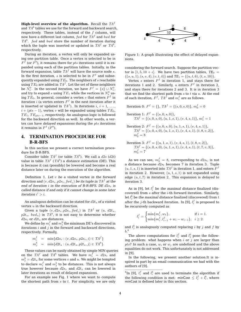
For an example see Fig. 1 where we want to computethe shortest path from s to t. For simplicity, we are only

Figure 1: A graph illustrating the effect of delayed expan-sions.

considering the forward search. Suppose the partition vec-tor is [1, 5, 10 + ε]. We have two partition tables, TE0 ={(s, u, 1), (s, v, 4), (v, t, 4)} and TE1 = {(u, t, 6), (t, s, 10)}.

Vertex s enters F f in iteration 1, and stays there foriterations 1 and 2. Similarly, u enters F f in iteration 2,and stays there for iterations 2 and 3. It is in iteration 3that we find the shortest path from s to t via u. At the endof each iteration, F f , TAf and mf

i are as follows.

Iteration 0: F f = {}, TAf = {(s, 0, s, 0)}, mf0 = 0

Iteration 1: F f = {(s, 0, s, 0)},TAf = {(s, 0, s, 0), (u, 1, s, 1), (v, 4, s, 1)}, mf

1 = 1

Iteration 2: F f = {(s, 0, s, 0), (u, 1, s, 1), (v, 4, s, 1)},TAf = {(s, 0, s, 0), (u, 1, s, 1), (v, 4, s, 1), (t, 8, v, 2)},mf

2 = 8

Iteration 3: F f = {(u, 1, s, 1), (v, 4, s, 1), (t, 8, v, 2)},TAf = {(s, 0, s, 0), (u, 1, s, 1), (v, 4, s, 1), (t, 7, v, 3)},mf

3 = 7

As we can see, mf2 = 8, corresponding to d2st, is not

a distance because d2st becomes 7 in iteration 3. Tuple(u, 1, s, 1) is inserted into TAf in iteration 1, and enters F f

in iteration 2. However, (u, 1, s, 1) is not expanded usingedge (u, t, 7) in iteration 2. This expansion is delayed toiteration 3.

As in [9], let lfi be the maximal distance finalized (dis-covered) from s after the i-th forward iteration. Similarly,let lbj be the maximal distance finalized (discovered) from t

after the j-th backward iteration. In [9], lfi is proposed tobe recursively computed as

lfi =

{min{mf

i , w1}, if i = 1.

min{mfi , l

fi−1 + wi − wi−1}, i ≥ 2.

and lbj is analogously computed replacing i by j and f byb.4

The above computations for lfi and lbj pose the follow-ing problem: what happens when i or j are larger thanpts? In such a case, wi or wj are undefined and the aboveequalities do not work. This unfortunately is not addressedin [9].

In the following, we present another solution.It is in-spired in part by an email communication we had with theauthors of [9].

4In [9], lfi and lbi are used to terminate the algorithm if

the following condition is met: minCost ≤ lfi + lbi , whereminCost is defined later in this section.

4

In fact, what we propose is computing lower bounds tolfi and lbj . We use llfi and llbj to denote the lower bounds for

lfi and lbj and set them to be as follows.

First, llf0 = lf0 = mf0 (= 0), llb0 = lb0 = mb

0(= 0), andllf1 = lf1 = mf

1 , llb1 = lb1 = mb1.

Now, let k = min{i− 1, pts} and h = min{j − 1, pts}. Fori, j ≥ 2, we set

llfi = min{mfi ,m

fi−1 + w1, . . . ,m

fi−k + wf

k} (1)

llbj = min{mbj ,m

bj−1 + w1, . . . ,m

bj−h + wb

h}. (2)

Suppose, for instance that i = 2, 3, 4, 5 and pts = 3.Then, k = 1, 2, 3, 3, and for the forward direction, we have

llf2 = min(mf2 ,m

f1 + w1)

llf3 = min(mf3 ,m

f2 + w1,m

f1 + w2)

llf4 = min(mf4 ,m

f3 + w1,m

f2 + w2,m

f1 + w3)

llf5 = min(mf5 ,m

f4 + w1,m

f3 + w2,m

f2 + w3).

We show the following theorem.

Theorem 1. llfi ≤ lfi and llbj ≤ lbj .

Proof. Consider llf2 . We have that mf2 is a distance of a

vertex v (from s) unless there exists a vertex u that hasremained with fwd = 1 after the 2nd iteration. Vertex udid not have any luck to be expanded by edges in [w0, w1),however, it may be expanded by edges in the next intervaland possibly cause the DE of v to get lower. In this case,the distance of v should be at least mf

1 + w1(< mf2 ).

Now consider llfi . We have that mfi is a distance of a

vertex v (from s) unless there exists a vertex u that hasremained with fwd ≤ i− 1 after the i-th iteration. Supposeu has fwd = i− 1. As such, u did not have any luck to joinwith edges in [w0, w1), however again, it may be expandedby edges in the next interval and possibly cause the DE ofv to get lower. In this case, the distance of v should be atleastmf

i−1+w1(< mfi ). Similarly, suppose u has fwd = i−r,

for r ∈ [1, k]. As such, u did not have any luck to joinwith edges in [w0, w1),. . . , [wr−1, wr), however, it may beexpanded by edges in the next interval and possibly causethe DE of v to get lower. In this case, the distance of vshould be at least mf

i−r + wr(< mfi ). From all the above,

llfi ≤ lfi .

An analogous argument can be made for the backwarddirection as well.

Remark. We would like to emphasize here thatmfi ’s (mb

j ’s)

are each time recomputed. For example, mf2 is recom-

puted when computing llf3 . This is because the vertexachieving the old mf

2 might have been updated in the cur-rent iteration and can now have fwd > 2. Therefore an-other vertex with fwd = 2 will provide the new mf

2 . Thenew mf

2 is greater than the old one.

For the termination decision we define

minCost =

{min{d2sv + d2tv}, if TAf 1nid TA

b 6= ∅∞, otherwise.

(3)

Now, we give the following condition that we use in thetermination procedure.

minCost ≤ llfi + llbj . (4)

If the above condition 4 is true, then by Theorem 1, thefollowing condition is true as well.

minCost ≤ lfi + lbj . (5)

If the last condition is true, then we can safely terminateB-R-BFS (see [9]). Upon such termination, minCost willbe the length of the shortest path from the source to thetarget vertex. In other words, even though we might nothave computed yet lfi and lbj , we can infer that Condition 5is satisfied based on Condition 4 using the lower boundsllfi and llbj .

With the modified termination condition provided in thissection, each vertex in the shortest path p takes pts itera-tions to finalize, hence the algorithm is estimated to takelength(p) ∗ pts iterations.

5. BIDIRECTIONAL LEVEL-BASED- FRON-TIER BFS (B-LF-BFS)

Here we propose another set-at-a-time algorithm for com-puting shortest paths in RDBMS. Similarly to B-R-BFS, itworks in a set-at-a-time fashion by expanding a set of ver-tices in each iteration. Differently from B-R-BFS, it achievesrestrictive expansions not by splitting the edge table, butby selecting only a part of the visited vertices as a frontierto be expanded. The algorithm performs better in practicethan B-R-BFS and it does not require partitioning the TEtable into several tables as in B-R-BFS. This can be desir-able as it does not need extra space for partition tables andcode complexity is reduced.

The Bidirectional Level-based-Frontier BFS (B-LF-BFS)we propose uses the TE , TAf and TAb tables as definedbefore. We do not need to record the iteration number asin B-R-BFS, and we bring back the finalization flag f inTAf and TAb.

We define F f = F fi , where F f

i is the set of all the ver-tices in TAf that are not finalized and their d2s value isless or equal to Li, where Li is a distance level. We defineF b in an analogous way.

For the sake of explanation, let us assume we are work-ing in the forward direction and that initially we set L1 =step, where step is a small constant. Now the algorithmwill (a) expand all the vertices in F f (i.e. unfinalized ver-tices in TAf that have d2s ≤ L1), (b) merge all the newvertices into TAf , then (c) iterate and do the same, untilno more unfinalized vertices with d2s ≤ L1 exist in TAf . Atthis point we say that level L1 is cleared, set L2 = L1+step,and repeat the above operations for L2.

In general, once level Li is cleared, we set Li+1 = Li +step, and repeat the above operations for Li+1. This con-tinues until termination is achieved. The algorithm termi-nates when a vertex v is finalized by both the forward andbackward directions, or if there are no more unfinalizedvertices in TAf or TAb.

Now, we illustrate the algorithm with an example. Forthe sake of simplicity we will explain the forward expan-sion; the backward expansion is similar. Consider the graph

5

in Figure 1 and assume step = 3. In order to calculatethe shortest distance between s and t, we initialize L1 =step = 3, minCost = ∞, and the TAf table with the tu-ple (s, s, 0, false). In the first iteration, the algorithm willexpand the initial tuple in TAf with d2s = 0 ≤ L1 andf f = false. So, node s will be expanded and nodes u withd2s=1 and v with d2s=4 will be merged into TAf and nodes will be flagged as processed (its flag f f becomes true).The algorithm will iterate to check if there are any tuplesin TAf with d2s ≤ L1 and f f = false. Node u with d2s = 1will be expanded and as a result node t with d2s = 6 willbe merged into TAf . At this point, no more nodes withd2s ≤ L1 are left to be processed, hence the algorithm de-clares that L1 is cleared and sets L2 = L1 + step = 6. Asnode t is merged, the algorithm sets minCost = 6. Next,the algorithm will expand the nodes that have not beenprocessed yet and have d2s ≤ L2. As a result, node v withd2s = 4 will be expanded resulting in rediscovering nodet with higher cost d2s = 8, hence no tuple will be mergedin TAf . As no more nodes are left to process, level L2 iscleared. At this point, node t will be flagged as finalized.

MERGE INTO TAf

USING (

WITH

--Compute frontier

F(nid,p2s,d2s) AS (

SELECT nid, p2s, d2s

FROM TAf

WHERE f_f='0' AND d2s <= Li

),

--Join frontier with the edge table

F_TE(nid,p2s,d2s) AS (

SELECT TE.tid AS nid, TE. d AS p2s, F.d2s+TE.cost AS d2s

FROM F JOIN TE ON F.nid=TE. d

),

--For each nid, select the tuple with the smallest d2s value

SELECT nid, p2s, d2s

FROM (SELECT nid, p2s, d2s,

row_number() OVER

(PARTITION BY nid ORDER BY d2s) AS rn

FROM F_TE)

WHERE rn = 1

) source

ON (TAf.nid=source.nid)

WHEN MATCHED THEN

UPDATE SET d2s=source.d2s, p2s=source.p2s, f_f='0'

WHERE source.d2s<TAf.d2s

WHEN NOT MATCHED THEN

INSERT (nid,d2s,p2s,f_f)

VALUES (source.nid, source.d2s, source.p2s, '0');

--Node �nalization

UPDATE TAf SET f_f='1' WHERE f_f='0' AND d2s <= Li;

Figure 2: SQL statements for the B-LF-BFS algorithm.

More formally, we give the following definitions for B-LF-BFS.

Definition 2. The F f and F b sets in levels Li and Lj are

F fi = {(nid, d2s, p2s, f f ) ∈ TAf : f f = 0 and d2s ≤ Li}

F bj = {(nid, d2t, p2t, f b) ∈ TAb : f b = 0 and d2t ≤ Lj}.

Consider F fi , for some i ≥ 1. The algorithm expands the

vertices in F fi , then recomputes F f

i . We give the followingdefinition.

Definition 3. We say that level Li, for i ≥ 1, is clearedin the forward direction, if F f

i is empty. Likewise, levelLj , for j ≥ 1, is cleared in the backward direction, if F b

j isempty.

Theorem 2. If level Li is cleared in the forward direc-tion, then the d2s values in TAf , such that d2s ≤ Li, arefinal and represent distances to the source vertex s.

Proof.Suppose not, i.e. let us assume there exists a vertex

v ∈ V processed in level Li and assigned a d2s value d, butin a later level, Li′ > Li, v is assigned a lower d2s valued′ < d. Vertex v will be discovered in level Li′ through avertex, say u, not processed in iteration Li, which impliesthat vertex u has a d2s value greater than Li, therefored′ > Li > d, which is a contradiction.

Similarly, we can show that

Theorem 3. If level Lj is cleared in the backward di-rection, then the d2t values in TAb, such that d2t ≤ Lj , arefinal and represent distances to the target vertex t.

Once we clear a level Li (Lj), we finalize all the verticesin TAf (TAb) with d2s ≤ Li (d2t ≤ Lj). We finalize thosevertices by setting their f f or f b flag to 1 (true). Observethat as we go to the next level, Li+1 (Lj+1), the set F f

i+1

(F fi+1) will contain those vertices of TAf (TAb) that are un-

finalized and have a d2s value less than Li+1 (Lj+1). Since,all the vertices of TAf (TAb) with d2s ≤ Li (d2t ≤ Lj)have been finalized, we have that in level Li+1 (Lj+1), weonly process vertices of TAf (TAb) with Li < d2s ≤ Li+1

(Lj < d2t ≤ Lj+1).In the B-LF-BFS algorithm, we have a clear way to fi-

nalize vertices, hence the termination decision becomeseasier; it happens when we find a vertex that is finalizedby both the forward and backward directions, or if thereare no more unfinalized vertices in TAf or TAb. The va-lidity of this condition for any bidirectional shortest-pathalgorithm (that finalizes vertices) is shown in [18]. In con-trast, we did not have the ability to easily decide how tofinalize vertices in B-R-BFS, hence, we had to resort to amuch more complex termination procedure.

The computed F f and F b sets in B-LF-BFS are only apart of the TAf or TAb tables. Therefore the joins withthe TE table are restricted in size compared to a full BFSapproach.

Whereas B-R-BFS achieves the join reduction by parti-tioning the TE table, B-LF-BFS achieves a similar effectby performing first a selection on the TAf and TAb tablesto generate a smaller set to join with TE .

The pseudo-code for clearing a level in B-LF-BFS in theforward direction is given in Algorithm 1. Please refer toFig. 2 for the SQL statements. Once a level is cleared, wego to the next level until no more expansions are possible.The backward direction is analogous. B-LF-BFS alternatesbetween the forward and backward direction depending

6

Algorithm 1 B-LF-BFS expand and merge

1: function ExpandAndMerge(TAf , TE , Li)2: do3: Compute F f

i (view F)4: Join F f

i with TE (view F_TE)5: For each nid in F_TE,6: compute the tuple with the smallest d2s7: Merge all the tuples thus produced into TAf

8: n← number of merged tuples9: while n 6= 010: Finalize all vertices in TAf with f f = 0 and d2s ≤ Li

11: end function

on the number of tuples merged in TAf and TAb choosingeach time the direction with the fewer merges.

The computations in lines 3–7 of Algorithm 1 are imple-mented by the SQL MERGE statement in Fig. 2. There, wefirst create two views, F and F_TE.5 View F contains setF f . View F_TE contains the join of F f with TE .

Next, for each vertex id, nid, we compute the tuple withthe smallest d2s in F_TE. For this we use the row_number()SQL window function6. Then comes the merge of thus ob-tained tuples into table TAf . If we obtained a tuple thatis better (with respect to d2s) than a tuple with the samenid in TAf , then the latter will be replaced by the former.Also, the tuples that do not have counterparts in TAf (withrespect to nid) will be simply inserted into TAf .

Finally, we finalize all the vertices in TAf with f f = 0 (f_f= ‘0’) and d2s ≤ Li. The finalization of vertices (tuples) inTAf is done by setting the value of their f f flag (f_f) in TAf

to 1. This is done with the last SQL statement in Fig. 2.Now we analyze the number of iterations the algorithm

would take. Suppose first we only do forward search. Letmc > 0 be the cost of the lightest edge in the graph. Letmp be the cost of the shortest path from s to t. In orderto clear a level, we need dmp/stepe iterations in the worstcase. In order to discover the shortest path from s to t,we need dmp/stepe levels in the worst case. Therefore,we need d(mp/step)e ∗ (step/mc) iterations in the worstcase. When we do bidirectional search, we will need abouthalf this number of iterations. This analysis shows thatthe algorithm terminates in a finite number of iterations.Based on the above reasoning and Theorem 2, we concludethe correctness of the algorithm.

6. B-LF-BFS WITH COMPRESSED ADJA-CENCY LISTS (B-LF-BFS-C)

In this section, we present B-LF-BFS-C, which enhancesB-LF-BFS using a compressed representation of the inputgraph.

A RDBMS often uses more space than necessary for stor-ing numeric datatypes (cf. [22]). Also, an edge table,such as TE , has unnecessary redundancy. For example,if a highly connected vertex v has, say 1000 neighbors,

5We are calling F and F_TE “views”, however, they aremore precisely called “factored subqueries” (created withthe SQL keyword WITH).6See https://en.wikipedia.org/wiki/Select_(SQL)

u1, . . . , u1000, then v’s id will repeat 1000 times to repre-sent the 1000 edges that connect v to its neighbors, i.e. wewill have the triples (v, u1, c1), (v, u2, c2), . . . , (v, u1000, c1000).

A better alternative is to use an adjacency list of neigh-bors and costs, e.g. for v, we would have a list such as[u1, c1, u2, c2, . . . , u1000, c1000]. While this is an improve-ment, we can do better than just storing the numbers intheir original form. In fact, we can compress an adjacencylist quite efficiently.

We borrow the idea of variable-byte-encoding of postingslists from Information Retrieval practice (cf. [28, 3, 46]).A posting list for a term is a list of documents that containthe term. For example, for a term, say dog, we can havea posting list like [334, 345, 350], where the numbers aredocument ids containing dog. Observe that document idsare sorted in ascending order.

There is a similarity between a posting list and an adja-cency list; instead of document ids we have neighbor ids.

For representing a posting list, we do not store the origi-nal document ids; rather, we store the gaps (or differences)between document ids. So, in the previous example, theposting list becomes [334, 11, 5], where 11 is 345− 334, and5 is 350 − 345. Now, variable-byte encoding is used forthe modified posting list. Specifically, we need 2 bytes for334, and only one byte for each of the other two numbers,for a total of 4 bytes. In contrast, the original posting list,with fixed-byte-encoded integers of, say 4 bytes, needs 12bytes.

We applied this idea for encoding the graph adjacencylists. We stored the obtained byte-encodings as BLOB’s(Binary Large Objects) in the TE table. More specifically,the TE table has now only two attributes, fid (as before)and ncb (which stands for neighbor-cost bytestream).

The pseudo-code for encoding/decoding sorted adjacencylists is given in algorithms 2, 3, and 4.

A number is encoded by a list of bytes. The rightmost 7bits in a byte are content and represent a part of the num-ber. The leftmost bit is an indicator flag. If it is 1, it meansthat the byte is the last one in the number encoding. If itis 0, it means there are more bytes following up in the en-coding. In Algorithm 3, we encode a list of neighbor/costnumbers. We iterate over the elements of this list in pairsof neighbor and cost. We encode the difference of the cur-rent neighbor from the previous one, then encode the costof the edge reaching the neighbor. When decoding a list ofbytes (see Algorithm 4), we check for the leftmost bit of thebytes we read in order to detect the end of a number en-coding. To decode a number, we extract and put togetherthe 7 rightmost bits of the bytes in its encoding. We alsocheck to see if the number we decoded is a neighbor (gap)or a cost, and proceed accordingly.

Expansion. In the following we describe the forward ex-pansion. The backward version is analogous. The set F f

is computed using a similar query as before (see view F inFig. 3). The join of F f with TE returns now a result setof (nid, ncb, d2s) tuples. The ncb value is a list of bytes en-coding the neighbors of nid and the costs to reach theseneighbors. The d2s value represents the distance estima-tion of nid from the source vertex.

7

Algorithm 2 Encoding of a number a

1: function encode(a)2: bytelist ← ∅3: do4: bytelist ← bytelist .prepend(a & 0x7F)5: a← a >> 76: while a > 07: bytelist [bytelist .size] = bytelist [bytelist .size] | 0x808: return bytelist9: end function

Algorithm 3 Encoding of a list of neighbor/cost numbers

1: function encode(list)2: bytelist ← ∅3: prev_neighbor ← 04: for each neighbor , cost in list do5: δ ← neighbor − prev_neighbor6: bytelist1 ← encode(δ)7: bytelist2 ← encode(cost)8: bytelist .concatenate(bytelist1)9: bytelist .concatenate(bytelist2)10: prev_neighbor ← neighbor11: end for12: return bytelist13: end function

Algorithm 4 Decoding of a list of bytes bytelist

1: function decode(bytelist)2: list ← ∅, a← 03: prev_neighbor ← 0, is_neighbor ← true4: for each byte in bytelist do5: if byte < 0x80 then6: a← a << 7 | byte7: else8: byte ← byte & 0x7F9: a← (a << 7) | byte10: if is_neighbor = true then11: a← prev_neighbor + a12: prev_neighbor ← a13: is_neighbor ← false14: else15: is_neighbor ← true16: end if17: list .append(a)18: a← 019: end if20: end for21: return list22: end function

The neighbor-cost byte lists in the join result need to bedecoded first in order to obtain tuples that can be mergedinto TAf . This is done by a procedure described in Al-gorithm 5. In this procedure, we populate a new table,EX f (nid, d2s, p2s), which will contain the tuples that willbe merged into TAf . We truncate (clean-up) this table ateach expansion round.

After performing the clean-up of EX f (first statement

in Fig. 3), then the computation of F f , and the join withTE , the procedure proceeds with the creation of the tuplesfor EX f . Specifically, for each tuple in the join result, itdecodes the ncb byte list and iterates over the producednumbers. The iteration is done in pairs a, b to account forneighbor id and cost (a is neighbor id, b is cost). Let t bethe current tuple being processed from the join result. Thed2s and p2s values of the new tuple we create are set to bet.d2s+ b and t.fid, respectively.

Finally, once we populate the EX f table, we merge itwith TAf using the SQL MERGE statement in Fig. 3. Dif-ferently from Fig. 2, the view creations in Fig. 3 are notpart of the MERGE statement. Within the MERGE state-ment, for each nid, we first compute the tuple with thesmallest d2s in EX f . Then, we proceed with the merge ofthese tuples into TAf . The vertex finalization query is thesame as in Fig. 2. The main algorithm for clearing a givenlevel is shown in Algorithm 6.

--Prepare the EXf table for a fresh expansion

TRUNCATE TABLE EXf;

WITH

--Compute frontier

F(nid,p2s,d2s) AS (

SELECT nid, p2s, d2s

FROM TAf

WHERE f_f='0' AND d2s <= Li

),

--Join frontier with the edge table

F_TE(nid,ncb,d2s) AS (

SELECT TE. d, TE.ncb, TA.d2s

FROM F JOIN TE ON F.nid=TE. d

),

SELECT * FROM F_TE;

--Merge into TAf

MERGE INTO TAf

USING (

--For each nid, select the tuple with the smallest d2s value

SELECT nid, p2s, d2s

FROM (SELECT nid, p2s, d2s,

row_number() OVER

(PARTITION BY nid ORDER BY d2s) AS rn

FROM EXf)

WHERE rn = 1

) source

ON (TAf.nid=source.nid)

WHEN MATCHED THEN

UPDATE SET d2s=source.d2s, p2s=source.p2s, f_f='0'

WHERE source.d2s<TAf.d2s

WHEN NOT MATCHED THEN

INSERT (nid,d2s,p2s,f_f)

VALUES(source.nid, source.d2s, source.p2s, '0')

Figure 3: SQL statements for B-LF-BFS-C.

7. EXPERIMENTAL RESULTSSetup. All our experiments are conducted on a consumer-grade machine with Intel i7, 3.4Ghz CPU, and 12Gb RAM,running Windows 7 Professional. The hard disk is Sea-gate Barracuda ST31000524AS 1TB 7200 RPM. We usedthe latest versions of two commercial databases (which weanonymously call D1 and D2) as well as PostgreSQL 9.4.4(PG).

We performed our analysis on six real and ten syntheticgraph datasets. We show the results for the real datasetsin Fig. 4 and for synthetic datasets in Fig. 5.

8

Algorithm 5 Populating expansion table EX f

1: procedure populate(EX f , TAf , TE , Li)2: EX f ← ∅ (truncate statement in Fig. 3)3: Compute F f

i (view F in Fig. 3)4: Join F f

i with TE (view F_TE in Fig. 3)5: for each t in F_TE do6: list ← decode(t.ncb)7: for each a, b in list do8: nid← a, d2s← t.d2s+ b, p2s← t.fid9: Insert (nid, d2s, p2s) into EX f

10: end for11: end for12: end procedure

Algorithm 6 B-LF-BFS-C expand and merge

1: function ExpandAndMerge(TAf , TE , Li)2: do3: populate(EX f ,TAf ,TE , Li)4: Merge EX f into TAf (MERGE in Fig.3)5: n← number of merged tuples6: while n 6= 07: Finalize all vertices in TAf with f f = 0 and d2s ≤ Li

8: end function

The real datasets are Web-Google, Pokec, Live-Journal(all three from http://snap.stanford.edu), and UK 2002,Arabic 2005, UK 2005 (all three from http://law.di.unimi.it/webdata).

The characteristics of the real datasets are as follows.

Name # of vertices # edges DiameterWeb-Google 875,713 5,105,039 21Pokec 1,632,803 30,622,564 11Live Journal 4,847,571 68,993,773 16UK 2002 18,520,486 298,113,762 21Arabic 2005 22,744,080 639,999,458 22UK 2005 39,459,925 936,364,282 23

The last three datasets, UK 2002, Arabic 2005, and UK2002 are significantly bigger than the first three as well asthe datasets considered in [9]. UK 2005, for instance, hasclose to one billion edges. We give a bar chart of the edgenumbers in Fig. 4d.

The synthetic datasets vary in size from 1 million edgesto 15 million edges. We generated five random graphs withsizes of 1, 2, 5, 10, and 15 million edges (denoted by 1M,2M, 5M, and 15M), and five graphs of the same sizes usingthe preferential attachment model.

In figures 5b, 5c, and 5d, we compare the performanceof B-R-BFS, B-LF-BFS, and B-LF-BFS-C on random vs. pref-erential attachment graphs. We see that their performanceon the two types of graphs is more or less the same. There-fore, we show results using random graphs in the rest ofthe charts of Fig. 5.

For edge weights, we generated random numbers from1 to 100 using uniform distributions for both real and syn-thetic datasets.

Regarding indexes we experimented with clustered andnon- clustered indexes on the edge table. The results using

clustered indexes are better (see figures 5k and 5l). Forthe TA tables, we did not create indexes as this sloweddown the MERGE operations and the performance of allthe algorithms suffered.

Each running time is given in seconds and obtained asan average over 100 random s-t queries.

In the following, we give the questions we aim to addresswith our experiments.

Questions.

Q1 How scalable are the algorithms we consider? How dothey compare to each other? In particular, can theyhandle large and very large graphs, e.g. Live Journal(large) and UK 2005 (very large)?

Q2 How well do the algorithms perform against baselines,such as the following variants of the bidirectional Di-jkstra’s algorithm: (a) in memory (when the graphfits there), (b) in RDBMS, and (c) in a modern nativegraph database (Neo4j)?

Q3 What are the best parameters for B-R-BFS, B-LF-BFS,and B-LF-BFS-C (number of partitions, p, for the first,and step size, s, for the second and third)?

Q4 What is the processing time trend as the size of thedataset grows?

Q5 What is the relative cost of database operations?

Q6 Is there a notable difference in the particular RDBMSchosen for this problem?

Answers.

Q1. In figures 4a and 5a, we show the running times ofthe algorithms under their best parameter setup. For B-R-BFS, the datasets are partitioned into 5, 10, and 15 ta-bles (p=5, p=10, p=15), respectively, and for B-LF-BFSand B-LF-BFS-C, step is set to 1,2 and 3 (s=1,s=2,s=3),respectively. Fig. 4a shows the running times for the realdatasets, whereas Fig. 5a for the synthetic ones (all ob-tained using D2).

We see that B-LF-BFS outperforms B-R-BFS on all thedatasets, with the difference being more pronounced forthe random graphs. Recall though that our main contribu-tion in B-LF-BFS is simplicity over B-R-BFS both in termsof algorithmic design as well as termination detection. Thefact that B-LF-BFS performs better than B-R-BFS showsthat we achieved simplicity without sacrificing performance.

B-LF-BFS-C outperforms both B-LF-BFS and B-R-BFS,and the difference becomes quite significant for Live Jour-nal. This behavior of B-LF-BFS-C is due to the fact thatmany fewer disk blocks are needed to store the TE tableusing the compression presented in Section 6. Therefore,there are less disk blocks to read to perform the main join.To see the compression achieved, please refer to Fig. 4lthat shows the sizes of original and compressed TE ta-bles for various datasets (using D2, the best performingRDBMS). The compression is quite significant for all thedatasets, and for some, such as Arabic 2005 and UK 2005,it is by a factor of more than 20. This compression ra-tio shows that our compression is quite efficient; it also

9

(a) Algorithms under theirbest parameter settings.

(b) B-LF-BFS-C, differentstep sizes, big graphs

(c) B-LF-BFS-C vs. base-lines.

(d) Graph sizes in millionsof edges (for reference).

(e) B-R-BFS, different parti-tion numbers.

(f) B-LF-BFS, different stepsizes.

(g) B-LF-BFS-C, differentstep sizes.

(h) B-LF-BFS-C {s=1}, dif-ferent RDBMSs.

(i) B-LF-BFS-C, differentstep sizes, big graphs, D1.

(j) B-LF-BFS-C, differentstep sizes, big graphs, PG.

(k) Buffer size influence onrun. time (B-LF-BFS-C).

(l) Original vs. CompressedTE (megabytes).

Figure 4: Experimental results for real datasets. All values on the vertical axes are times in seconds, except for 4d and 4l.

shows that there is a blowup factor when storing data un-compressed in a database. For example the CSV edge fileof UK 2005 is 38 GB, which is less than half the size of theTE table (78 GB) for the same dataset. A similar blowuphas also been observed in other works, e.g. [22].

Regarding UK 2002, Arabic 2005, and UK 2005, B-LF-BFS-C is the only one to be able to handle them (see Fig. 4b).In fact, B-LF-BFS-C does on UK 2005 significantly better(by more than 27%) than what the other two algorithmscan do for Live Journal, which is an order of magnitudesmaller than UK 2005. B-R-BFS and B-LF-BFS were notable to handle the three largest datasets in our machinein a reasonable time; for instance, it took B-LF-BFS abouttwo hours to compute a single s-t query on UK 2002.

We observe that the average time for B-LF-BFS-C is only3.7 seconds on Live Journal, and 12.4 seconds on UK 2005.Fig. 4k shows the running time of B-LF-BFS-C on UK 2005for different buffer allocations. We see there is only mildimprovement as the buffer size grows. This applies to allthree RDBMSs we used (D1, D2, PG). We discuss perfor-mance comparisons among RDBMSs later in this section.

Q2. Regarding the baselines, we show the results in Fig. 4c.We compare there the baselines against each other andB-LF-BFS-C. As expected, the in-memory implementationof bidirectional Dijkstra’s algorithm (B-D-InMem) is fasterthan its counterparts in RDBMS (B-D) and Neo4j. Also ex-

pected is the fact that B-LF-BFS-C does quite better thanB-D and Neo4j; this is because B-LF-BFS-C benefits from aset-at-a-time approach (see Section 3.2 for a discussion).What is quite revealing though is that B-LF-BFS-C is aclose contender to B-D-InMem and even outperforms it onLive Journal. This affirms the virtue of set-at-a-time eval-uation, intelligent scheduling by the RDBMS, and graphcompression in B-LF-BFS-C.

Q3. Now we focus on what the best parameters for theconsidered algorithms are. We see in Fig 4e that p = 5is the best number of partitions for B-R-BFS in the realdatasets. This is also confirmed by Fig. 5e for syntheticdatasets. For the latter, we only show lines for p = 5 andp = 10 as the numbers for p = 15 were too large to beinteresting. We explain this behavior of B-R-BFS as fol-lows. While having more partitions (edge tables) helps topotentially achieve termination faster using the early joins(those using low-numbered edge tables), there is neverthe-less an added penalty in terms of page scheduling by theRDBMS, if we are to join the same part of the F set with toomany edge tables (which happens when the finalization isdelayed). In other words, joins become too-small-too-many,and the performance suffers.

In Fig. 4f and 5f we see the B-LF-BFS performance fordifferent step values on the real and synthetic datasets, re-spectively. We see that s = 1 is the best value for B-LF-BFS.

10

(a) Algorithms under theirbest parameter settings.

(b) B-R-BFS, pref. attach-ment and random graphs.

(c) B-LF-BFS, pref. attach-ment and random graphs.

(d) B-LF-BFS-C, pref. at-tach. and rand. graphs.

(e) B-R-BFS, different par-tition numbers.

(f) B-LF-BFS, differentstep sizes.

(g) B-LF-BFS-C, differentstep sizes.

(h) B-LF-BFS-C, windowfunctions vs. classicalSQL.

(i) B-LF-BFS, differentRDBMSs.

(j) B-LF-BFS-C, differentRDBMSs.

(k) B-LF-BFS, non-cluster.and cluster. ind.

(l) B-LF-BFS-C with non-cluster. and cluster. ind.

Figure 5: Experimental results for synthetic datasets. All values on the vertical axes are times in seconds.

Whereas the differences in running time for s = 1, 2, 3 arenot big for the real datasets, they become quite noticeablefor the synthetic datasets. For the latter, the performancefor s = 1 is significantly better than for s = 2, 3. Recall thatthe greater the step size, the bigger the F sets become,and the more the B-LF-BFS gets closer to BFS. For B-LF-BFS-C, on the other hand, we find that s = 3 is the bestvalue for the three big real datasets (Fig. 4b), whereas s =1 is the best value for the medium real datasets (Fig. 4g)and synthetic datasets (Fig. 5g). This suggests that someparameter tuneup is needed depending on the graph.

The tuneup of the step size can be performed by ran-domly selecting a set of source-target pairs as we are doingin our experiments. Then, we test different values for stepstarting from a value equal to the cost of the lightest edgeand incrementing it by this amount each time. What welook for is some value for the step size such that the set-at-the-time evaluation has an opportunity to better scheduledisk accesses while not doing too much non-optimal work.As our experiments show, moderate values for the step sizegive a good balanced evaluation.

Q4. In Fig. 5a, we see that the curve for B-R-BFS, even forp = 5, grows faster compared to B-LF-BFS and B-LF-BFS-C. This trend for B-R-BFS is more pronounced in Fig. 5e for

p = 10. The curve for B-LF-BFS grows in general mildly,unless its step value is not tuned properly (see Fig. 5f).Finally, B-LF-BFS-C has the mildest growing curve of thethree algorithms and is somewhat “forgiving” even when sis not tuned to the best value (see Fig. 5g).

Q5. The experiments in Fig. 6 were conducted using syn-thetic data sets (random graphs of 1-15 million edges) withstep = 3. Fig. 6a shows the relative time for finding fron-tier nodes versus and the time taken for executing thejoin queries in B-LF-BFS. The Merge time was not consid-ered in the figure as it was insignificant. We can see thatthe processing time is mainly consumed by join queries.Fig. 6b shows the relative time for B-LF-BFS-C to decodecompressed tuples in table TE, find frontier nodes, andexecute join queries. We can see that decoding did notconsume the significant portion of the whole processingtime. It is still the join time that dominates.

Q6. Figures 4h and 5j show the performance of differ-ent RDBMSs when running B-LF-BFS-C (best algorithm).We allocated the same amount of buffer space, 6G, andcreated the same index setup for all three of RDBMSs weused. We see that D1 and Postgres performed similarly,however, D2 significantly outperformed both of them. A

11

(a) (b)

Figure 6: Relative cost of different database operations.

similar behavior can also be observed when running B-LF-BFS (see Fig. 5i).

To better see the performance of B-LF-BFS-C on differ-ent RDBMSs, we also give figures 4i (for D1) and 4j (forPostgres), which should be compared with Fig 4b (for D2).

These results suggest that even though well-developedRDBMSs (such as those we consider) are close competitorsin well-known benchmarks, when it comes to handling spe-cialized workloads (such as graph operations), they shownoticeable differences.

8. RELATED WORKComputing s-t queries on large complex networks has

received considerable attention from the research com-munity (cf. [1, 2, 23] and [6, 15, 29, 31, 42]). The firstand second group of works compute exact and approxi-mate answers, respectively. As we provide exact answersto s-t queries, our work is more related to the first group.The works in the first group achieve very good scalabil-ity, but focus on unweighted graphs, which is an easierproblem to tackle. In unweighted graphs, the length ofa path amounts to the number of its edges. Since so-cial and web graphs have typically a small diameter, com-puting s-t shortest paths on unweighted graphs does notneed to travel more than few hops. On the other hand,if edge weights are taken into consideration, the smalldiameter of the graphs is not that important anymore asshortest paths can contain an arbitrary number of edges,hence, many more expansions are needed. In this paper,in contrast with the aforementioned works, we focus onweighted graphs, which are more general and challengingto handle. While we do not show experimental resultsfor unweighted graphs, we mention that we tested exten-sively with such graphs in RDBMS and our performancewas considerably better than for weighted graphs.

Bidirectional computation for finding shortest paths froma source to a target has been suggested in several works(cf. [11, 18]. In [18], it is shown that proper terminationis when both the forward and backward search finalize agraph vertex in common. Recall, this was possible for thebidirectional Dijkstra’s algorithm and B-LF-BFS, but notfor B-R-BFS (for which we need to resort to a more com-plex termination procedure). In [11], the benefits of bidi-rectional search are shown by experiments for graphs thatfit in memory. Another part of [11] is about A* heuristicsfor speeding up the s-t shortest path computation. Suchheuristics, however, were in practice observed in [11] to

be mainly useful for spatial networks (and not much forcomplex networks). In this paper, we focus on complexnetworks (social and web networks). As such, we have notemployed A* heuristics.

Relational Databases have been often used to store com-plex data, such as XML and RDF graphs (cf. [5, 32] and [4,17], respectively). They have also been shown to be a goodchoice to support advanced applications, such as data min-ing [34, 45] and machine learning [10, 25].

For graph queries, as [16, 43] argue, relational technol-ogy can sometimes outperform more specialized solutions.An interesting work that uses relational technology for an-swering subgraph and supergraph queries is [33]. Thesequeries are different from our source-to-target shortestpath queries. Other works, such as [8, 24] use rela-tional databases to build vertex-centric (VC) systems in thePregel model. As we explained in Section 2, a VC compu-tation is not a good fit for computing s-t shortest paths.In terms of table structure, the edge tables used in B-R-BFS and B-LF-BFS are similar to the edge table in [8]. Allthese works (including ours) suggest that using relationaldatabases for graph management can be for some prob-lems better than using specialized graph engines.

9. CONCLUSIONSWe showed that designing algorithms for RDBMS is a

good avenue to pursue for graphs that do not fit in mem-ory, and sometimes, even for graphs that can (e.g. LiveJournal). Also, RDBMS technology is quite mature and canaccommodate complex data and algorithms, sometimes,even better than special purpose systems.

We presented a correct procedure for deciding termina-tion in B-R-BFS. We argued that it is challenging to de-termine whether a vertex has its distance finalized in B-R-BFS. Then we showed that we can decide termination bycarefully deriving lower bounds on the forward and back-ward distances of vertices from the source and target.

We gave next a new algorithm, B-LF-BFS, which per-forms restrictive BFS by selecting only a part of the visitedvertices as a set to be expanded. This was achieved by set-ting distance levels that need to be cleared (in terms of ex-pansions) before going to the next level. We showed that,once a level is cleared, the vertices that were expanded inthat level have their distance finalized. This allowed us touse a much simplified termination procedure.

Then, we presented B-LF-BFS-C, an algorithm that en-hances B-LF-BFS by using a compressed representation ofneighbor-cost lists. The compression achieved was suchthat B-LF-BFS-C was able to handle graphs of an order ofmagnitude bigger than what B-R-BFS and B-LF-BFS could.

Using detailed experiments, we showed that all three al-gorithms scale well (for their best parameter setup), andB-LF-BFS-C in particular can produce results in a reason-able time even on the largest dataset we experimentedwith, UK 2005, with close to one billion edges, using onlya consumer-grade machine.

As future work, we would like to extend our results usingRDBMS to shortest paths in graphs that are both weightedand labeled with symbols from a finite alphabet [12, 35,40]. In this case, the paths allowed to follow are specified

12

by regular expressions and the goal is to compute shortestpaths that spell words in the query language [13, 14, 39].

10. REFERENCES[1] R. Agarwal, M. Caesar, P. B. Godfrey, and B. Y. Zhao.

Shortest paths in less than a millisecond. In ACMWorkshop on Online Social Networks. ACM, 2012.

[2] T. Akiba, Y. Iwata, and Y. Yoshida. Fast exactshortest-path distance queries on large networks bypruned landmark labeling. In SIGMOD. ACM, 2013.

[3] V. N. Anh and A. Moffat. Inverted index compressionusing word-aligned binary codes. InformationRetrieval, 8(1):151–166, 2005.

[4] H. Chen, Z. Wu, H. Wang, and Y. Mao. Rdf/rdfs-basedrelational database integration. In ICDE, pages94–94. IEEE, 2006.

[5] L. J. Chen, P. Bernstein, P. Carlin, D. Filipovic,M. Rys, N. Shamgunov, J. F. Terwilliger, M. Todic,S. Tomasevic, D. Tomic, et al. Mapping xml to a widesparse table. Knowledge and Data Engineering,IEEE Transactions on, 26(6):1400–1414, 2014.

[6] A. Das Sarma, S. Gollapudi, M. Najork, andR. Panigrahy. A sketch-based distance oracle forweb-scale graphs. In WSDM. ACM, 2010.

[7] E. W. Dijkstra. A note on two problems in connexionwith graphs. NUMERISCHE MATHEMATIK,1(1):269–271, 1959.

[8] J. Fan, A. G. S. Raj, and J. M. Patel. The case againstspecialized graph analytics engines. In CIDR, 2015.

[9] J. Gao, J. Zhou, J. X. Yu, and T. Wang. Shortest pathcomputing in relational dbmss. IEEE Trans. Knowl.Data Eng., 26(4):997–1011, 2014.

[10] W. Gatterbauer, S. Günnemann, D. Koutra, andC. Faloutsos. Linearized and single-pass beliefpropagation. PVLDB, 8(5):581–592, 2015.

[11] A. V. Goldberg and C. Harrelson. Computing theshortest path: A search meets graph theory. InSODA, pages 156–165, 2005.

[12] G. Grahne and A. Thomo. Query answering andcontainment for regular path queries underdistortions. In International Symposium onFoundations of Information and Knowledge Systems,pages 98–115. Springer, 2004.

[13] G. Grahne and A. Thomo. Regular path queries underapproximate semantics. Annals of Mathematics andArtificial Intelligence, 46(1-2):165–190, 2006.

[14] G. Grahne, A. Thomo, and W. Wadge. Preferentiallyannotated regular path queries. In InternationalConference on Database Theory, pages 314–328.Springer, 2007.

[15] A. Gubichev, S. Bedathur, S. Seufert, and G. Weikum.Fast and accurate estimation of shortest paths inlarge graphs. In CIKM, pages 499–508. ACM, 2010.

[16] A. Gubichev and M. Then. Graph pattern matching:Do we have to reinvent the wheel? In Proceedings ofWorkshop on GRAph Data management Experiencesand Systems, pages 1–7. ACM, 2014.

[17] S. Harris and N. Shadbolt. Sparql query processingwith conventional relational database systems. In

Web Information Systems Engineering–WISE 2005Workshops, pages 235–244. Springer, 2005.

[18] M. Holzer, F. Schulz, D. Wagner, and T. Willhalm.Combining speed-up techniques for shortest-pathcomputations. ACM Journal of ExperimentalAlgorithmics, 10, 2005.

[19] J. E. Hopcroft and R. E. Tarjan. Efficient algorithmsfor graph manipulation. 1971.

[20] H.-P. Hsieh, C.-T. Li, and R. Yan. I see you:Person-of-interest search in social networks. InSIGIR, pages 839–842. ACM, 2015.

[21] S.-W. Huang, D. Tunkelang, and K. Karahalios. Therole of network distance in linkedin people search.In SIGIR, pages 867–870. ACM, 2014.

[22] A. Jacobs. The pathologies of big data.Communications of the ACM, 52(8):36–44, 2009.

[23] R. Jin, N. Ruan, Y. Xiang, and V. Lee. Ahighway-centric labeling approach for answeringdistance queries on large sparse graphs. InSIGMOD, pages 445–456. ACM, 2012.

[24] A. Jindal, P. Rawlani, E. Wu, S. Madden,A. Deshpande, and M. Stonebraker. Vertexica: yourrelational friend for graph analytics! PVLDB, 2014.

[25] M. L. Koc and C. Ré. Incrementally maintainingclassification using an rdbms. PVLDB, 4(5):302–313,2011.

[26] A. Kyrola, G. E. Blelloch, and C. Guestrin. Graphchi:Large-scale graph computation on just a pc. In OSDI,volume 12, pages 31–46, 2012.

[27] G. Malewicz, M. H. Austern, A. J. Bik, J. C. Dehnert,I. Horn, N. Leiser, and G. Czajkowski. Pregel: asystem for large-scale graph processing. InSIGMOD, pages 135–146. ACM, 2010.

[28] C. D. Manning, P. Raghavan, and H. Schütze.Introduction to information retrieval. Cambridgeuniversity press, 2008.

[29] M. Potamias, F. Bonchi, C. Castillo, and A. Gionis.Fast shortest path distance estimation in largenetworks. In CIKM, pages 867–876. ACM, 2009.

[30] R. C. Prim. Shortest connection networks and somegeneralizations. Bell system technical journal,36(6):1389–1401, 1957.

[31] M. Qiao, H. Cheng, L. Chang, and J. X. Yu.Approximate shortest distance computing: Aquery-dependent local landmark scheme. IEEETrans. Knowl. Data Eng., 26(1):55–68, 2014.

[32] M. Rys, D. Chamberlin, and D. Florescu. Xml andrelational database management systems: the insidestory. In SIGMOD, pages 945–947. ACM, 2005.

[33] S. Sakr and G. Al-Naymat. Efficient relationaltechniques for processing graph queries. Journal ofComputer Science and Technology,25(6):1237–1255, 2010.

[34] X. Shang, K. U. Sattler, and I. Geist. Sql basedfrequent pattern mining without candidategeneration. In SAC, pages 618–619. ACM, 2004.

[35] M. Shoaran and A. Thomo. Fault-tolerantcomputation of distributed regular path queries.

13

Theoretical Computer Science, 410(1):62–77, 2009.

[36] P. Singla and M. Richardson. Yes, there is acorrelation:-from social networks to personalbehavior on the web. In WWW. ACM, 2008.

[37] C. Sommer. Shortest-path queries in static networks.ACM Computing Surveys (CSUR), 46(4):45, 2014.

[38] N. V. Spirin, J. He, M. Develin, K. G. Karahalios, andM. Boucher. People search within an online socialnetwork: Large scale analysis of facebook graphsearch query logs. In CIKM. ACM, 2014.

[39] D. Stefanescu and A. Thomo. Enhanced regular pathqueries on semistructured databases. InInternational Conference on Extending DatabaseTechnology, pages 700–711. Springer, 2006.

[40] D. C. Stefanescu, A. Thomo, and L. Thomo.Distributed evaluation of generalized path queries.In Proceedings of the 2005 ACM symposium onApplied computing, pages 610–616. ACM, 2005.

[41] G. Swamynathan, C. Wilson, B. Boe, K. Almeroth,and B. Y. Zhao. Do social networks improvee-commerce? a study on social marketplaces. InFirst Workshop on Online Social Net. ACM, 2008.

[42] K. Tretyakov, A. Armas-Cervantes,L. García-Bañuelos, J. Vilo, and M. Dumas. Fast fullydynamic landmark-based estimation of shortest pathdistances in very large graphs. In CIKM, pages1785–1794. ACM, 2011.

[43] A. Welc, R. Raman, Z. Wu, S. Hong, H. Chafi, andJ. Banerjee. Graph analysis: do we have to reinventthe wheel? In First International Workshop on GraphData Manag. Experiences and Systems. ACM, 2013.

[44] S. A. Yahia, M. Benedikt, L. V. Lakshmanan, andJ. Stoyanovich. Efficient network aware search incollaborative tagging sites. PVLDB, 1(1), 2008.

[45] B. Zou, X. Ma, B. Kemme, G. Newton, and D. Precup.Data mining using relational database managementsystems. In Advances in Knowledge Discovery andData Mining, pages 657–667. Springer, 2006.

[46] M. Zukowski, S. Heman, N. Nes, and P. Boncz.Super-scalar ram-cpu cache compression. In ICDE,pages 59–59. IEEE, 2006.

14