computing geodesics in numerical space times · computing geodesics in numerical space times de...
TRANSCRIPT

Leopold-Franzens University InnsbruckInstitute of Computer Science
Computing Geodesics in NumericalSpace Times
De computatione distantiarum brevissimarumin spatiis quattuor dimensionum numeris
descriptis
Master Thesis
Marcel Ritter
Supervisor: O. Univ. Prof. Dr. Sabine Schindler
March 30, 2010

*
In memoriam:
O. Univ. Prof. i.R. Dr. sub ausp. Manfred Ritter
Who never lost his curiosity, fascination and deep passion for science andteaching even during difficult circumstances.
Although he was unable to support my work in this world I know hisguiding spirit was always by my side.

2
Figure 1: Geodesics in a Kerr metric.
Abstract:
Traditionally, tools to visualize geodesics in curved spacetimes of general rel-ativity have been specialized solutions, either tailored to a certain spacetimeor limited to certain kinds of numerical data. Utilizing a Fiber Bundle datamodel and the Vish visualization environment, this thesis aims to solve thisproblem by developing an approach that is independent of the underlyingnumerical data. My approach allows the combination of several visualizationmodules, and opens the possibility of applying the computation and visu-alization of integral lines more readily to other scientific domains. Thesedomains include computational fluid dynamics and medical imaging.

Contents
1 Introduction 6
2 Theoretical Background 102.1 Differential Geometry . . . . . . . . . . . . . . . . . . . . . . . 10
2.1.1 Manifolds and Charts . . . . . . . . . . . . . . . . . . . 102.1.2 Curve . . . . . . . . . . . . . . . . . . . . . . . . . . . 122.1.3 Tangential Vector . . . . . . . . . . . . . . . . . . . . . 12
Transformation . . . . . . . . . . . . . . . . . . . . . . 132.1.4 Covector . . . . . . . . . . . . . . . . . . . . . . . . . . 132.1.5 Tensor Field . . . . . . . . . . . . . . . . . . . . . . . . 142.1.6 Metric . . . . . . . . . . . . . . . . . . . . . . . . . . . 152.1.7 Geodesic Equation and Christoffel Symbols . . . . . . . 16
Geodesic Equation . . . . . . . . . . . . . . . . . . . . 16Christoffel Symbols . . . . . . . . . . . . . . . . . . . . 19
2.1.8 Geodesic Deviation and Riemann Tensor . . . . . . . . 202.1.9 Ricci Tensor and Scalar . . . . . . . . . . . . . . . . . 21
2.2 General Relativity . . . . . . . . . . . . . . . . . . . . . . . . 222.2.1 Einstein Field Equation . . . . . . . . . . . . . . . . . 222.2.2 Schwarzschild Metric . . . . . . . . . . . . . . . . . . . 232.2.3 Kerr Metric . . . . . . . . . . . . . . . . . . . . . . . . 24
2.3 Fluid Dynamics . . . . . . . . . . . . . . . . . . . . . . . . . . 262.4 Medical Imaging . . . . . . . . . . . . . . . . . . . . . . . . . 28
3 Implementation Concepts 293.1 Type Traits . . . . . . . . . . . . . . . . . . . . . . . . . . . . 293.2 STL Encapsulation . . . . . . . . . . . . . . . . . . . . . . . . 333.3 Reference Pointers . . . . . . . . . . . . . . . . . . . . . . . . 33
4 Modeling of Scientific Data 364.1 Fiber Bundle Data Model . . . . . . . . . . . . . . . . . . . . 374.2 The Hierarchy Levels . . . . . . . . . . . . . . . . . . . . . . . 38
3

CONTENTS 4
4.2.1 Fiber Bundle . . . . . . . . . . . . . . . . . . . . . . . 384.2.2 Fiber Slice . . . . . . . . . . . . . . . . . . . . . . . . . 394.2.3 Fiber Grid . . . . . . . . . . . . . . . . . . . . . . . . . 404.2.4 Fiber Topology . . . . . . . . . . . . . . . . . . . . . . 414.2.5 Fiber Representation . . . . . . . . . . . . . . . . . . . 424.2.6 Fiber Field . . . . . . . . . . . . . . . . . . . . . . . . 43
4.3 Simplified Access via Selectors . . . . . . . . . . . . . . . . . . 464.4 Data Examples . . . . . . . . . . . . . . . . . . . . . . . . . . 47
4.4.1 Uniform, procedural . . . . . . . . . . . . . . . . . . . 484.4.2 Multiblock, Curvilinear . . . . . . . . . . . . . . . . . . 494.4.3 Lines . . . . . . . . . . . . . . . . . . . . . . . . . . . . 50
5 Vish - The Vis(h)ualization Environment 525.1 Development Quick Start . . . . . . . . . . . . . . . . . . . . . 53
5.1.1 Availability and Installation . . . . . . . . . . . . . . . 535.1.2 Source Code Organization and Naming Conventions . . 545.1.3 Make Files and Compilation . . . . . . . . . . . . . . . 56
5.2 Scene Network . . . . . . . . . . . . . . . . . . . . . . . . . . . 575.2.1 Modules . . . . . . . . . . . . . . . . . . . . . . . . . . 585.2.2 Data Transport and Access . . . . . . . . . . . . . . . 62
Creating new Parameter Types . . . . . . . . . . . . . 62Fiber Bundle Data Access . . . . . . . . . . . . . . . . 63
5.2.3 Rendering Modules . . . . . . . . . . . . . . . . . . . . 65Geometric Algebra . . . . . . . . . . . . . . . . . . . . 66OpenGL . . . . . . . . . . . . . . . . . . . . . . . . . . 67Using OpenGL in a Rendering Module . . . . . . . . . 67
5.2.4 Vish Scripts . . . . . . . . . . . . . . . . . . . . . . . . 725.3 Caching . . . . . . . . . . . . . . . . . . . . . . . . . . . . . . 755.4 Data Field Interpolation and Finding Local Coordinates . . . 77
5.4.1 UniGrid . . . . . . . . . . . . . . . . . . . . . . . . . . 795.4.2 Multiblock . . . . . . . . . . . . . . . . . . . . . . . . . 805.4.3 Curvilinear . . . . . . . . . . . . . . . . . . . . . . . . 85
Local Coordinates in one Hexahedral Cell . . . . . . . 86Finding Candidates in the Grid . . . . . . . . . . . . . 89Summarizing the Steps . . . . . . . . . . . . . . . . . . 91
5.5 Basic Visualization Modules . . . . . . . . . . . . . . . . . . . 935.5.1 Coordinate Grid . . . . . . . . . . . . . . . . . . . . . 935.5.2 Coordinate Grid Box . . . . . . . . . . . . . . . . . . . 945.5.3 Uniform Grid Lines . . . . . . . . . . . . . . . . . . . . 955.5.4 Color Map Legend . . . . . . . . . . . . . . . . . . . . 955.5.5 Multiblock Outlines . . . . . . . . . . . . . . . . . . . . 97

CONTENTS 5
6 Computation and Visualization 996.1 Defining Initial Conditions for Integral Lines . . . . . . . . . . 100
6.1.1 Initial Positions, Seed Points . . . . . . . . . . . . . . . 100Geometric Point Distributions . . . . . . . . . . . . . . 101Random Point Distribution . . . . . . . . . . . . . . . 105Grid Union, Convolution and Transformation . . . . . 107
6.1.2 Defining Initial Directions . . . . . . . . . . . . . . . . 111Grid Subtraction . . . . . . . . . . . . . . . . . . . . . 111
6.2 Computation . . . . . . . . . . . . . . . . . . . . . . . . . . . 1126.2.1 Computing First Order Integration Lines . . . . . . . . 1216.2.2 Computing Second Order Integration Lines . . . . . . . 126
6.3 Rendering Lines . . . . . . . . . . . . . . . . . . . . . . . . . . 134
7 Applications 1417.1 Visualizing Flow of CouetteFlow . . . . . . . . . . . . . . . . . 1427.2 Visualizing Flow and Pressure in a Stirred Fluid Tank . . . . . 1497.3 Visualizing Geodesics in a sampled Schwarzschild Metric . . . 1607.4 Visualizing Geodesics in a sampled Kerr Metric . . . . . . . . 1797.5 Fiber Tracking in MRI Data . . . . . . . . . . . . . . . . . . . 205
8 Future Work 209
9 Conclusion 211
10 Fazit 213
A Acknowledgements 221
B Definition of Fiber Bundles 222
C Related Publications 223

Chapter 1
Introduction
The objective of this thesis is to provide a visualization framework suitablefor exploring numerical spacetimes originating from astrophysical numericalrelativity.
Numerical relativity is a very active research area. Having immense com-puting power available, numerical methods allow to solve the Einstein fieldequations, chapter 2.2.1, as is was not possible before. One specific applica-tion is the detection of gravitational waves. Gravitational waves have not yetbeen directly measured, but a Nobel Prize was given to Hulse and Taylor,[44], for finding a convincing indirect evidence. They measured timings ina binary pulsar. The observed frequency increase can only be explained byenergy loss due to the emission of gravitational waves. Thus, the waves them-selves have not yet been measured, but their effect on the emitting systemshas been observed. Gravitational waves are ripples in spacetime curvaturepropagating with the speed of light. “Any mass in nonspherical, nonrecti-linear motion produces gravitational waves (...), but gravitational waves areproduced most copiously in events such as the coalescence of two compactstars, the merger of massive black holes, or the big bang.” [36]
Detectors for gravitational waves have been built in the United States inLivingston, Louisiana, in Hanford, Washington [39], in Europe in Hannover,Germany [29], and near Pisa, Italy [24]. In order to detect a gravitationalwave, relative distance changes in the order of 10−22 have to be measured.
Numerical analysis of situations involving strong gravity, such as themerging of black holes is of great importance. These simulations can beused to match the actually measured data of the gravitational wave detec-tors. Interactive 3D visualization techniques based purely on numerical datahelps to analyze these simulations. This thesis focuses on the visualization ofgeodesics, the shortest (or longest) path between points in space (or space-time). They are important indicators of the structure of spacetime.
6

CHAPTER 1. INTRODUCTION 7
Geodesics in curved spacetimes have been studied before, but most workis related to the visualization of analytic spacetimes, 1992 [2], 1997 [26], 1999[22], 2001 [15] and 2004 [28]. Computing geodesics is required for ray-tracingblack holes. In 1991 Corvin Zahn at the University of Tubingen implementedfour dimensional ray-tracing in an analytic Schwarzschild space time, [63].The most similar work was done already in 1992 by Steve Bryson, who im-plemented geodesic visualizations for exploration using a “boom mounted sixdegree of freedom head position sensitive stereo CRT system”, [17]. For hissetup the curved spacetimes could be given by closed formulas or also onsimple uniform grids.
Geodesics were also analyzed in numerical spacetimes in the 2D (axisym-metric) era. The famous “pair of pants” picture contains the event horizonin a head-on collision, along with some geodesics. The corresponding movieswere made in 1995 with great effort in TV resolution, see e.g. [43]. WernerBenger at the University of Innsbruck simulated a black hole by raytracingin 1996 [4]. Andrew Hamilton implemented a real time flight simulator for acharged black hole. He uses a projective technique to compute the paths ofgeodesics, [35].
Spacetimes visualized in this thesis are sampled on uniform grids. How-ever, the developed infrastructure used in this work easily extends to adaptivemesh refinement (AMR) grids, which are currently used for numerical simu-lations of merging and colliding black holes, without changing the computa-tion and visualization algorithms. Moreover, the rudimentary visualizationof geodesics can be enhanced with other visualization modules, for instanceto show the coordinate-acceleration, equation (2.53), on the geodesics.
Inspired by Bryson’s seeding methods for geodesics I developed a flexibletechnique for the creation of seeding geometries using basic operating blocksbased on the theory of fiber bundles, that can be combined to a huge varietyof seeding geometries.
In addition to the visualization and computation, other aspects have beenaddressed in this work:
the data model
high code re-usability
high modularity
provide an introduction to utilized software environments and libraries
The modern scientific world uses many computational methods in differentscientific domains. The requirement of collaborations increases and thus

CHAPTER 1. INTRODUCTION 8
exchanging data becomes important. During my research visit at LouisianaState University I was taught that in 2005 hurricane Katrina forced scientificgroups to exchange their data sets and couple different kinds of numericsimulations to predict the path of Katrina to provide warning and rescue tothe public. For example, actual satellite data was coupled with simulation ofthe motion of air of the hurricane, which was then coupled with a simulationfor wave propagation on the ocean. Such coupling is only possible if datacan be exchanged without time-consuming data conversion processes betweenthe different scientific groups. The simulation results were later gatheredin a visualization combining several layers stemming from all the differentdomains, [14].
The thesis starts with a short theoretical part providing the necessarymathematical and physical background of general relativity, computationalfluid dynamics and magnetic resonance imaging needed for the visualizationand interpretation of the resulting illustrations, chapter 2.
Thereafter, some C++ programming techniques used for implementationare presented in chapter 3. Template meta programming is covered for en-hancing overall source code re-usability.
Chapter 4 introduces and describes the concepts of the data model usedthroughout this thesis. Utilizing this data model made it possible to easilyapply the developed algorithms to other applications such as medical imag-ing. It also enhanced source code re-usability because algorithms could bereused in situations that had not been possible without such a strong conceptat the software foundation level.
Chapter 5 introduces the visualization environment that was used to im-plement the algorithms. It consists of a very flexible and modular system ofsoftware components that can be easily extended. During the implementa-tion several parts of the software environments were refined and additionalfeatures where added to the software kernel.
The core work of the thesis is described in chapter 6. Concepts and al-gorithms for computing geodesics and streamlines are presented there andfinally verified and utilized in chapter 7. The initial objective of comput-ing geodesics was widened to the computation of integral lines. A simplerapplication scenario was chosen to develop the basic software infrastructure,which was later extended to the final application. Especially during the workon the foundations, it was possible to apply some of the new techniques incollaborative work that led to publications, appendix C.
A clarifying review of the available infrastructure was essential for thesuccess of this work. While creating a tutorial and complementing program-ming and user documentation of the research I got the necessary insights todevelop the key concepts of the visualization framework. Still there is no good

CHAPTER 1. INTRODUCTION 9
overall getting-started-documentation for someone who also might want toutilize the visualization and data environments as yet, because it is researchsoftware and no commercial environment. I decided to give quite detaileddescriptions and source code excerpts throughout the thesis. Thus, manyparts of the thesis can also be read as an introductory to the visualizationenvironment Vish and the Fiber Bundle data library.

Chapter 2
Theoretical Background
This chapter briefly captures the mathematical and physical background ofthe thesis. It follows the descriptions of [55], [36], [6], [5], [38],[54], [47] and[40], which were adapted to the requirements of the thesis.
Following notations were used:
Einstein summing convention is used. Same indices occurring at upperand lower position are summed up: ανβ
ν = α1β1 + α2β
2 + . . .
Partial derivation is written as index: ∂f∂x
:= f,x
2.1 Differential Geometry
2.1.1 Manifolds and Charts
Let S be a set. Then P(S) is the set of all subsets of S, called the powerset of S. [49]
Let X be a set ∧ P be the power set. A subset τ ⊆ P(X) is a topologyif:
arbitrary unions of elements of τ are contained in τ , i.e. if I is anarbitrary (also infinite) set of indices and ∀i ∈ I : Ui ∈ τ then
⋃i∈I Ui ∈
τ ,
finite intersections of elements of τ are contained in τ , i.e. if U0, U1,..., Un ∈ τ then
⋂ni=0 Ui ∈ τ with n = N,
the empty set and the set X itself are contained in τ , i.e. ∅, X ∈ τ
The pair (X, τ) of a set X together with a topology τ on this set is a topo-logical space. The elements of a topological space are called points. [6]
10
CHAPTER 2. THEORETICAL BACKGROUND 11
Two topological spaces X, Y are homeomorphic, if there exists a bijec-tive map H : X → Y such that open sets of X are mapped to open sets inY and vice versa, i.e. the neighborhood relations must be sustained underthis mapping.H is called homeomorphism or topological map.
A topological space X is a Hausdorff space iff for any two distinct pointsx, y ∈ X there exist two distinct neighborhoods Ux, Uy such that Ux ∩ Uy =.
A manifold is a Hausdorff space that is locally homeomorphic to Eu-clidean space Rn.
A manifold is a topological space which locally looks like the Rn with theusual topology [54].
A chart is a xµ bijective and differentiable mapping (a diffeomorphism)from a point P of a manifold M to a n-tuple of scalar numbers.
q : M → Rn
P 7→ (xµ(P ) (2.1)
The numbers xµ(p) are called the coordinates of the point p in the chartxµ and xi is the ith coordinate function. [6] A chart that does not coverthe complete manifold M is called a local chart.
Later, spherical and Cartesian charts are used to represent the metric ofcurved space times. The spherical chart xµ, with x1 ≡ x, x2 ≡ y andx3 ≡ z, is transformed to Cartesian chart xµ, with x1 ≡ r, x2 ≡ θ andx3 ≡ φ:
x(r, θ, φ) = r · sinθ · cosφy(r, θ, φ) = r · sinθ · sinφz(r, θ, φ) = r · cosθ
(2.2)
And the transformation from xµ to xµ is:
r(x, y, z) =√x2 + y2 + z2
θ(x, y, z) = arctan
(√x2+y2
z
)
φ(x, y, z) =
π/2 : x = 0, y > 0
3π/2 : x = 0, y < 0
arctan yx
: x > 0
arctan yx
+ π : x < 0
(2.3)
CHAPTER 2. THEORETICAL BACKGROUND 12
2.1.2 Curve
A curve is a mapping from a scalar s ∈ R, the so called curve parameter, toa point on a manifold.
q : R → Ms 7→ q(s)
(2.4)
To describe a curve in a certain chart xµ the chart-function is used toextract a function for each coordinate of the chart:
qµ : R → Rs → qµ(s) = xµ(q(s)) ≡ xµ q(s) (2.5)
2.1.3 Tangential Vector
The tangential vector of a curve q(s) is defined by the operation dds
:
d
dsf(q(s)) := lim
h→0
f(q(s+ h))− f(q(s))
h(2.6)
In a certain chart xµ:d
dsf(q(s)) =
d
dsf(x0(q(s)), x1(q(s)), . . . ) =
∂f
∂xµdxµ(q(s))
ds(2.7)
=dxµ(q(s))
ds
∂
∂xµf
=dqµ(s)
ds
∂
∂xµf =: qµ(s)
∂
∂xµf
= f,µqµ
d
ds= qµ(s)
∂
∂xµ=: q (2.8)
The functions qµ are the components of the tangential vector in the chartxµ. If f is a chart-function xν , then d
dsis the νth component qν :
d
dsxν(q(s)) = qµ(s)
∂xν
∂xµ= q(s)δνµ = qν(s) (2.9)
The partial derivatives ∂∂xµ
span a vector space at a point P of a manifold M :the tangential vector space TP (M). Thus, the chart-functions xµ induce abasis ∂
xµ in TP (M).
∂µ :=∂
∂xµ(2.10)

CHAPTER 2. THEORETICAL BACKGROUND 13
Transformation
A tangential vector can be represented in different charts. For the basis ofthe tangential space ∂µ and the charts xµ and xµ
~∂ ≡ ∂
∂xµ=∂xµ
∂xµ· ∂
∂xµ=: αµµ · ~∂ (2.11)
with αµµ being the inner derivatives of the coordinate transformation:
αµµ = ∂xµ(xµ)∂xµ
and αµµ = ∂xµ(xµ)∂xµ
. (2.12)
Now, the tangential vector can be written as:
v = vµ∂µ = vµ∂µ = vµ(αµµ∂µ) (2.13)
It follows:
vµ = αµµvµ ∂µ = αµµ∂µ (2.14)
To fully describe the chart transformation αµµ(xµ), αµµ(xµ), αµµ(xµ) andαµµ(xµ) are needed, which can be written as transformation matrices.
One such transformation matrix is used in section 7.3 and section 7.4 totransform a metric given in spherical Coordinates to Cartesian coordinates.The according transformation matrix is:
αµµ(xµ) =
∂r∂x
= x√x2+y2+z2
∂r∂y
= y√x2+y2+z2
∂r∂z
= z√x2+y2+z2
∂θ∂x
= xz√x2+y2(x2+y2+z2)
∂θ∂y
= yz√x2+y2(x2+y2+z2)
∂θ∂z
= −√x2+y2
x2+y2+z2
∂φ∂x
= −yx2+y2
∂φ∂y
= xx2+y2
∂φ∂z
= 0
(2.15)
2.1.4 Covector
Let v ∈ TP (M) be a vector and f : M → R a real valued function on themanifold. Then applying the tangential vector vof f yields a number:
v(f) ∈ R (2.16)
Above we examined this expression for a fixed vector v and arbitrary functionf . Alternatively, we can study it for arbitrary v and fixed function f . Thisway it defines the function df which maps a tangential vector v to a numberdf(v) ∈ R:
df : TP (M) → Rv → df(v) := v(f)
(2.17)

CHAPTER 2. THEORETICAL BACKGROUND 14
The function df is called 1-form. 1-forms fulfill the vector space axioms:
(a·df+b·dg)(v) = v(a·f+b·g) = a·v(f)+b·v(g) = a·df(v)+b·dg(v) (2.18)
and thus span a vector space, called the cotangential space T ∗P (M). Itselements, calles covectors, are linear maps TP (M)→ R.
2.1.5 Tensor Field
Physical quantities are independent of an underlying coordinate system. Thisis known as the “principle of covariance”. Mathematically, tensors are usedto describe such quantities. A tensor can be written in any coordinate basis.The name tensor originates from its usage in continuum mechanics, where atensor of rank two is used to describe stresses, [40] or [41].
An m×n tensor F is a multilinear mapping from Cartesian products ofn tangential spaces TP (M) and m cotangential spaces T ∗P (M) into R at somepoint P of a manifold:
F : (TP (M))n × (T ∗P (M))mmultilinear
→ R (2.19)
m×n is the rank of the tensor. The vector space spanned by tensors is calledthe tensor product space
(T ∗P (M))⊗n⊗ (TP (M))⊗m := (TP (M))n× (T ∗P (M))mmultilinear
→ R, (2.20)
whereby X⊗n denotes the nth tensor product of the space X with itself. Dueto the duality relations T ∗P (M) ↔ TP (M), the tensor product space can beseen as the space of linear functions that map elements from the dual tensorproduct space to a number:
(T ∗P (M))⊗n⊗ (TP (M))⊗m = (TP (M))⊗n⊗ (T ∗P (M))⊗mlinear
→ R , (2.21)
With V, U two tensor product spaces, we see
V ⊗ U = V ∗ × U∗multilinear
→ R = V ∗ ⊗ U∗linear
→ R (2.22)
CHAPTER 2. THEORETICAL BACKGROUND 15
and
V ∗ ⊗ U∗ = V × Umultilinear
→ R = V ⊗ Ulinear
→ R (2.23)
It follows from equation (2.21) that V ∗ ⊗ U∗ ≡ (V ⊗ U)∗. [6]The tensor field t is a mapping from a point P of a manifold M to a
tensor in the tangential space TP (M).
t :M → (T ∗P (M))⊗n ⊗ (TP (M))⊗m (2.24)
Tensor fields are used in many physical and technical applications, for exam-ple, to describe distributions of temperature, velocity, stress or curvature inspace and time.
A tensor field of rank 0 × 0 is a scalar field M → R. A tensor field ofrank 0× 1 is a vector field v : M → TP (M). [6]A metric field is of rank 2× 0.
2.1.6 Metric
A metric G is a symmetric bilinear form on tangential vectors of a manifold.G is a bilinear mapping TP (M)×TP (M)→ R. With u, v, w being tangentialvectors, λ a scalar:
G(u+ λ · w, v) = G(u, v) + λ ·G(w, v)G(u, v + λ · w) = G(u, v) + λ ·G(u,w)
G(u, v) = G(v, u)(2.25)
In general relativity a metric tensor field is used to describe the curvature ofspacetime. The metric at one point of a manifold is represented as a 4 × 4matrix gµν . Because of its symmetry it has 10 independent components. Inthis work the signature (+,−,−,−) is used. Thus, the spatial componentshave a negative sign in contrast to the time components which are positive.
There exist three types of tangential vectors:
G(v, v) > 0↔ v is called time-like
G(w,w) = 0↔ w is called light-like
G(u, u) < 0↔ u is called space-like
CHAPTER 2. THEORETICAL BACKGROUND 16
The metric defines lengths of and angles between vectors. The length of atime-like tangential vector is
|v| :=√G(v, v) (2.26)
and of a space-like tangential vector it is
|u| :=√−G(u, u). (2.27)
The angle between two space-like tangential vectors is
cosα(u, v) :=G(u, v)
|u| · |v|=
G(u, v)√G(u, u) ·G(v, v)
(2.28)
A metric is written in a certain chart xµ as follows:
G(u, v) = G(uµ∂µ, vν∂ν) = uµ · vν ·G(∂µ, ∂ν) =: uµvνgµν (2.29)
For example, the metric tensor for flat space times in Cartesian and sphericalcoordinates are:
gµν =
1 0 0 00 −1 0 00 0 −1 00 0 0 −1
gµν =
1 0 0 00 −1 0 00 0 −r2 00 0 0 −r2sin2θ
(2.30)
If a metric is invertible the co-metric is defined via the Kronecker delta andis the inverse of the metric:
gµνgνλ = δλµ (2.31)
2.1.7 Geodesic Equation and Christoffel Symbols
Geodesic Equation
A geodesic is a curve with extremal length on a manifold. The length of acurve along a parameter interval s can be computed by integration using themetric tensor of equation (2.29):∫ s
0gq(σ)(q(σ), q(σ))︸ ︷︷ ︸ dσ
:= L(2.32)
To compute the extremum of the length we choose this expression as theLagrange function and compute the total differential:
dL =∂L∂sds+
∂L∂qk(s)
dqk(s) +∂L
∂qk(s)dqk(s) (2.33)

CHAPTER 2. THEORETICAL BACKGROUND 17
with:
dqk(s) = ∂qk(s)∂s
ds, ∂qk(s)∂s
= ˙qk(s) and qk(s) = xk(q(s)) (2.34)
dL =
(∂L∂s
+∂L∂xk
qk(s) +∂L
∂qk(s)qk(s)
)ds (2.35)
The partial derivative ∂L∂s
is 0, since L is not dependent on s. For minimizationwe claim:∫
dL =
∫ (∂L∂xk
qk(s) +∂L
∂qk(s)qk(s)
)ds = 0 (2.36)
Now we use partial integration on the second term in the integral of equation(2.36) to further simplify the equation:∫
f ′ g = f g −∫g f ′∫
qk(s) ∂L∂qk(s)
= qk(s) ∂L∂qk(s)
−∫
dds
∂L∂qk(s)
qk(s)(2.37)
Insertion of equation (2.37) in equation (2.36) yields:
= 0 = const∫ ︷ ︸︸ ︷∂L∂xk− d
ds
∂L∂qk(s)
qk(s)ds+
︷ ︸︸ ︷qk(s)
∂L∂qk(s)
= 0(2.38)
the last term in equation (2.38) is a constant term and thus must be 0. Also,the term in brackets () must be 0 because ∂L must be an extremum for anycurve q(s). This, simplifies the equation to:
∂L∂xk− d
ds
∂L∂qk(s)
= 0 (2.39)
We introduce coordinates and compute the terms of equation (2.39) usingthe Einstein notation :
L = gq(s)(q(s), q(s)) = gµν · qµ(s) · qν(s) (2.40)
First term of equation (2.39):
∂L∂xα
= L,α = gµν,αqµqν + gµν q
µ,αq
ν + gµν qµqν,α = gµν,αq
µqν + 2gµν qµ,α (2.41)
CHAPTER 2. THEORETICAL BACKGROUND 18
The metric tensor is symmetric. Thus coordinate indices may be flipped andthe two terms containing gµν be added. The term finally vanishes because:
qν,α = ∂qν
dxα= 0 → L
∂xα= gµν,αq
µqν (2.42)
Second term of equation (2.39):
= 0 = δµα = δνα
∂L∂qα(s)
=
︷ ︸︸ ︷∂gµνqα(s)
qµ(s)qµ(s) + gµν
︷ ︸︸ ︷∂qµ
qα(s)qν(s) + gµν q
µ(s)
︷ ︸︸ ︷∂qν
qα(s)
(2.43)
Again, using the symmetry of gµν :
∂L∂qα(s)
= gαν qν + gµαq
µ = 2gµαqµ (2.44)
d
ds
∂L∂qα(s)
= 2(d
dsgµαq
µ + gµαd
dsqµ) (2.45)
d
dsgµα =
∂gµα∂xν
d
dsqν = gµα,ν q
ν (2.46)
d
dsqµ = qµ (2.47)
d
ds
∂L∂qα(s)
= 2(gµα,ν qν qµ + qµqµ) (2.48)
All necessary terms are derived now. Insertion of equation (2.46) in equation(2.45) and further in equation (2.39) and equation (2.42) in equation (2.39):
gµν,αqµqν − 2(gµα,ν q
µqν + gµαqµ) = 0 (2.49)
−2gµαqµ − 2(gµα,ν −
1
2gµν,α)qµqν = 0| · (−1
2gαλ) (2.50)
qµ+1
2gαλ(2gµα,ν − gµν,α)︸ ︷︷ ︸ qµqν = 0
=: Aλµν
(2.51)
CHAPTER 2. THEORETICAL BACKGROUND 19
Introducing the abbreviationAλµν , where only the symmetric part contributes:
−q = Aλµν qµqν = Aλνµq
µqν = Aλνµqν qµ =
1
2(Aλµν + Aλνµ)︸ ︷︷ ︸ qν qµ
=: Γλµν
(2.52)
With Γλµν called the Christoffel Symbols, the final geodesic equation is:
qλ = Γλµν qµqν (2.53)
and Christoffel symbols:
Γλµν :=1
2gλα(
1
2(2gµα,ν − gµν,α) +
1
2(2gνα,µ − gνµ,α)
)(2.54)
Γλµν :=1
2gλα(gµα,ν + gνα,µ − gµν,α) (2.55)
The geodesic q(s) is an integral line because solving the equation (2.53)involves integration for computation. It is of second order since it is definedvia a second order derivative. To solve for q(s) the boundary conditions forq(0) and q(0) are required. The second derivative q can be interpreted as anacceleration. Since a geodesic represents an unaccelerated motion in curvedspacetime this term is more precisely called coordinate-acceleration.
Christoffel Symbols
To study the structure of Christoffel symbols four specific symbols are ex-panded. Here, it is assumed a 3D space. Consider a metric tensor g in xyzcoordinates. The dimension of g is 3×3 and we have to compute 3×3×3 = 27Christoffel symbols. Expanding Γλµν for λ = x, µ = x and ν = x for Γxxx yields:
Γxxx = 12[ gxx(gxx,x + gxx,x − gxx,x)+gxy(gxy,x + gxy,x − gxx,y)+gxz(gxz,x + gxz,x − gxx,z)]
(2.56)
Γxxx =1
2(gxx(gxx,x) + gxy(2gxy,x − gxx,y) + gxz(2gxz,x − gxx,z)) (2.57)
CHAPTER 2. THEORETICAL BACKGROUND 20
Next, three more Chirstoffel symbols are expanded varying just one index,e.g. λ = y, Γyxx yields:
Γyxx = 12[ gyx(gxx,x + gxx,x − gxx,x)+gyy(gxy,x + gxy,x − gxx,y)+gyz(gxz,x + gxz,x − gxx,z)]
(2.58)
Γyxx =1
2(gyx(gxx,x) + gyy(2gxy,x − gxx,y) + gyz(2gxz,x − gxx,z)) (2.59)
The Christoffel symbol with ν = y, Γxxy yields:
Γxxy = 12[ gxx(gxx,y + gyx,x − gxy,x)+gxy(gxy,y + gyy,x − gxy,y)+gxz(gxz,y + gyz,x − gxy,z)]
(2.60)
The Christoffel symbol with µ = y, Γxxy yields:
Γxyx = 12[ gxx(gyx,x + gxx,y − gyx,x)+gxy(gyy,x + gxy,y − gyx,y)+gxz(gyz,x + gxz,y − gyx,z)]
(2.61)
When comparing the terms of equation (2.56) and equation (2.58) it canbe seen that the terms in between the round brackets () remain unchanged,since they depend on indices µ and ν only. The same holds when comparingthe terms of equation (2.60) and equation (2.61). Because of the symmetryof the metric tensor gµν ( e.g. gxy,x == gyx,x ) the terms in round brackets() are equal.
Because of the symmetry property of the metric tensor also the Christof-fel Symbols are symmetrical. In the 3D case the number of independentcomponents is reduced from 27 to 18, in 4D from 64 to 40.
2.1.8 Geodesic Deviation and Riemann Tensor
The geodesic deviation describes the change in separation of neighboringgeodesics. The Riemann Tensor connects the deviation of the parallelism ofneighbored geodesics to the curvature of the spacetime:
Kγµδβ = Γγβµ,δ − Γγδµ,β + ΓκβµΓγδκ − ΓκδµΓγβκ (2.62)
The Riemann tensor is of rank four1 and has 44 components in R4. However,the number of independent components reduces to 20 when its symmetryproperties are analyzed, [38].
1or (1,3)

CHAPTER 2. THEORETICAL BACKGROUND 21
2.1.9 Ricci Tensor and Scalar
The Ricci tensor is the only not vanishing contraction of the Riemanntensor:
Rµν = Kκµκν (2.63)
The Ricci tensor is symmetric and has 10 independent components in R4.Geometrically interpreted it sums up curvatures of orthogonal geodesics sur-faces at an tangential vector v ∈ TP (M).
Further contraction of the Ricci tensor yields the so called Ricci scalar,which is an invariant of the Ricci tensor.
R = Rµµ (2.64)

CHAPTER 2. THEORETICAL BACKGROUND 22
2.2 General Relativity
In 1916 Albert Einstein introduced his relativistic theory of gravitation, see[25]. The general relativity describes gravity, which is the geometry of a fourdimensional spacetime. Due to the curved spacetime an object that experi-enced acceleration of a gravitational force in classical mechanics is unaccel-erated in general relativity. In fact it is just moving uniformly on a straightline, on a geodesic, but in a curved spacetime. Trajectories of photons andfree falling objects are represented by geodesics.
Using differential geometry, spacetime is described by an infinitesimalsmall line element specifying a distance between any two neighboring points.A four dimensional metric, section 2.1.6, is used for that purpose:
ds2 = gµνdxµdxν (2.65)
A metric tensor field describes the curvature at every point of the spacetimemanifold, section 2.1.6.
2.2.1 Einstein Field Equation
The heart of the general relativity theory is the equation that correlates mat-ter and energy with the spacetime curvature. It is known as the Einstein fieldequation. When a distribution of matter is given, the spacetime curvaturecan be computed by this equation.
Rµν −1
2gµνR = 8πGTµν (2.66)
The left hand side of equation (2.66) describes the curvature of spacetimeusing the Ricci tensor and the Ricci scalar, section 2.1.9. The right handside describes the distribution of matter by a tensor of rank two.
Tµν is called the energy-momentum-stress tensor and at it full complexitycaptures a scalar field for energy density, a vector field for the motion ofmatter, a scalar field for pressure, a space-like tensor field for stress and avector field for energy flux.
The equation (2.66) is a coupled system of differential equations of secondorder, which to the full extend can only be solved numerically. However, someanalytic solutions exist that make use of strong simplifications.
For example, for solutions in pure vacuum the equation simplifies toRµν = 0. The Schwarzschild metric and the Kerr metric are such analyticvacuum solutions of the Einstein field equation.

CHAPTER 2. THEORETICAL BACKGROUND 23
2.2.2 Schwarzschild Metric
“The solution of the field equations, which describe the field outside of aspherical symmetric mass distribution, was found by Karl Schwarzschild onlytwo months after Einstein published his field equations. ... From this solutionhe derived the precession of the perihelion of Mercury and the bending oflight rays at the surface of the sun.” [54]
The metric is expressed in spherical coordinates, with m being the massexpressed as a length:
m(in cm) := Gc2M(in g) (2.67)
g =
(1− 2m
r
)dt2 − dr2
1− 2m/r− r2(dθ2 + sin2θdφ2) (2.68)
To write g in matrix form the equation is expanded and the terms that aremultiplied by the squared derivatives are extracted:
g =
1− 2m
r0 0 0
0 −(1− 2m
r
)−10 0
0 0 −r2 00 0 0 −r2sin2θ
(2.69)
The according Christoffel symbols in polar coordinates are, [36]:
Γttr = (m/r2)(1− 2m/r)−1 Γθrθ = 1/rΓrtt = (m/r2)(1− 2m/r) Γθφφ = −cosθsinθΓrrr = −(m/r2)(1− 2m/r)−1 Γφrφ = 1/r
Γrθθ = −(r − 2m) Γφθφ = cotθ
Γrφφ = −(r − 2m)sin2θ
(2.70)
Important properties of the Schwarzschild Metric:
It is time independent and, thus, a stationary and static metric field.
It is spherically symmetric.
It has a singularity at r = 0 and r = 2m (Schwarzschild radius).
The radius of a static star is always outside the Schwarzschild radius. “TheSchwarzschild radius of the sun, for instance, is 2GM/c2 = 2.95 km - muchsmaller than the radius of the solar surface 6.96× 10⁵ km.” [36].
CHAPTER 2. THEORETICAL BACKGROUND 24
The singularity at r = 0 is a physical singularity at the center point.Here, curvature and mass becomes infinite.
The Schwarzschild radius is a singularity induced by the coordinate sys-tem. Other coordinates, such as Eddington-Finkelstein coordinates can beused to eliminate this singularity. However, it still has a physical meaning.Light rays or particles passing this radius towards the center cannot escapethe heavy mass. The surface at the Schwarzschild radius is called the eventhorizon of a black hole.
Properties of the Schwarzschild metric are explored by visualizinggeodesics in section 7.3.
2.2.3 Kerr Metric
The Kerr metric was discovered by Roy Kerr in 1963. They are a general-ization of the Schwarzschild metric by rotation. It can describe the actualendstate of collapsed astrophysical objects quite well. Besides the mass nowan additional parameter, the angular momentum, controls the spacetime ge-ometry. The so called “no hair theorem” states that at the endstate of acollapse only three quantities are conserved: the mass, the angular momen-tum and the electric charge, see [20].
“Yet the evidence of both theoretical investigation and numerical simula-tions is that the endstate of any realistic gravitational collapse that proceedsfar enough is remarkably simple, analogous in many ways to the special caseof spherical collapse. ...From the perspective of a distant observer, the endstate is indistinguishablefrom a time-independent Kerr black hole characterized by just mass M andangular momentum J, with a horizon that conceals the singularity in it. ...Kerr black holes thus provide the cleanest connection between fundamentalgravitational physics and realistic astrophysics.”[36]
The Kerr metric is formulated in Boyer-Lindquist coordinates, with:
a = J/M
∆ = r2 − 2Mr + a2 (2.71)
ρ2 = r2 + a2cosθ
The parameter a is called the Kerr parameter. If a = 0 then the Boyer-Lindquist coordinates are equivalent to the Schwarzschild coordinates. Themetric is:
g =∆
ρ2[dt−asin2θdφ]2− sin
2θ
ρ2[(r2 +a2)dφ−adt]2− ρ
2
∆dr2−ρ2dθ2 (2.72)
CHAPTER 2. THEORETICAL BACKGROUND 25
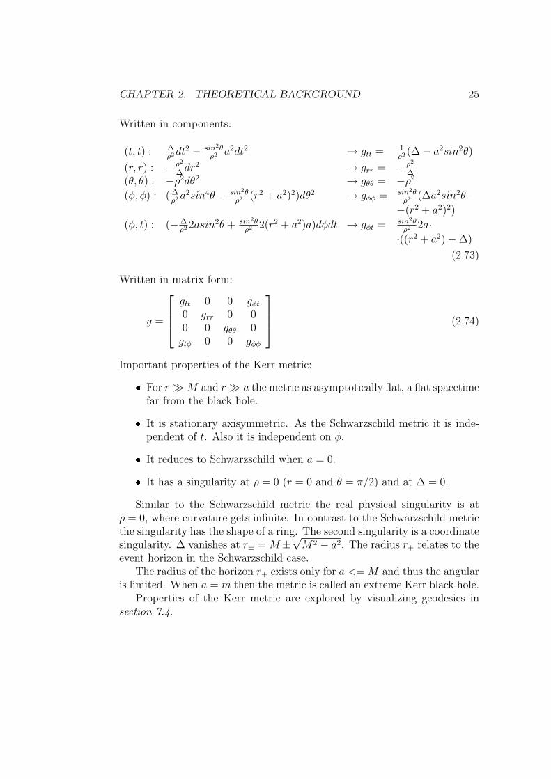
Written in components:
(t, t) : ∆ρ2dt
2 − sin2θρ2 a2dt2 → gtt = 1
ρ2 (∆− a2sin2θ)
(r, r) : −ρ2
∆dr2 → grr = −ρ2
∆
(θ, θ) : −ρ2dθ2 → gθθ = −ρ2
(φ, φ) : ( ∆ρ2a
2sin4θ − sin2θρ2 (r2 + a2)2)dθ2 → gφφ = sin2θ
ρ2 (∆a2sin2θ−−(r2 + a2)2)
(φ, t) : (−∆ρ2 2asin2θ + sin2θ
ρ2 2(r2 + a2)a)dφdt → gφt = sin2θρ2 2a··((r2 + a2)−∆)
(2.73)
Written in matrix form:
g =
gtt 0 0 gφt0 grr 0 00 0 gθθ 0gtφ 0 0 gφφ
(2.74)
Important properties of the Kerr metric:
For r M and r a the metric as asymptotically flat, a flat spacetimefar from the black hole.
It is stationary axisymmetric. As the Schwarzschild metric it is inde-pendent of t. Also it is independent on φ.
It reduces to Schwarzschild when a = 0.
It has a singularity at ρ = 0 (r = 0 and θ = π/2) and at ∆ = 0.
Similar to the Schwarzschild metric the real physical singularity is atρ = 0, where curvature gets infinite. In contrast to the Schwarzschild metricthe singularity has the shape of a ring. The second singularity is a coordinatesingularity. ∆ vanishes at r± = M ±
√M2 − a2. The radius r+ relates to the
event horizon in the Schwarzschild case.The radius of the horizon r+ exists only for a <= M and thus the angular
is limited. When a = m then the metric is called an extreme Kerr black hole.Properties of the Kerr metric are explored by visualizing geodesics in
section 7.4.
CHAPTER 2. THEORETICAL BACKGROUND 26
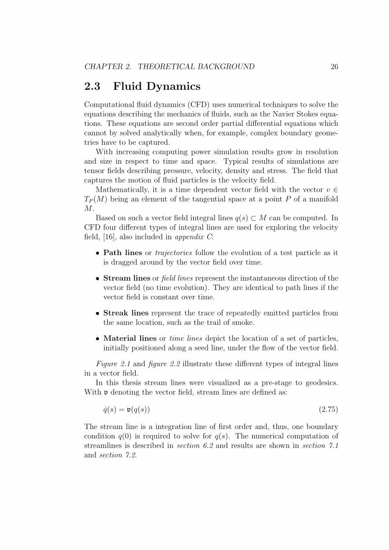
2.3 Fluid Dynamics
Computational fluid dynamics (CFD) uses numerical techniques to solve theequations describing the mechanics of fluids, such as the Navier Stokes equa-tions. These equations are second order partial differential equations whichcannot by solved analytically when, for example, complex boundary geome-tries have to be captured.
With increasing computing power simulation results grow in resolutionand size in respect to time and space. Typical results of simulations aretensor fields describing pressure, velocity, density and stress. The field thatcaptures the motion of fluid particles is the velocity field.
Mathematically, it is a time dependent vector field with the vector v ∈TP (M) being an element of the tangential space at a point P of a manifoldM .
Based on such a vector field integral lines q(s) ⊂M can be computed. InCFD four different types of integral lines are used for exploring the velocityfield, [16], also included in appendix C:
Path lines or trajectories follow the evolution of a test particle as itis dragged around by the vector field over time.
Stream lines or field lines represent the instantaneous direction of thevector field (no time evolution). They are identical to path lines if thevector field is constant over time.
Streak lines represent the trace of repeatedly emitted particles fromthe same location, such as the trail of smoke.
Material lines or time lines depict the location of a set of particles,initially positioned along a seed line, under the flow of the vector field.
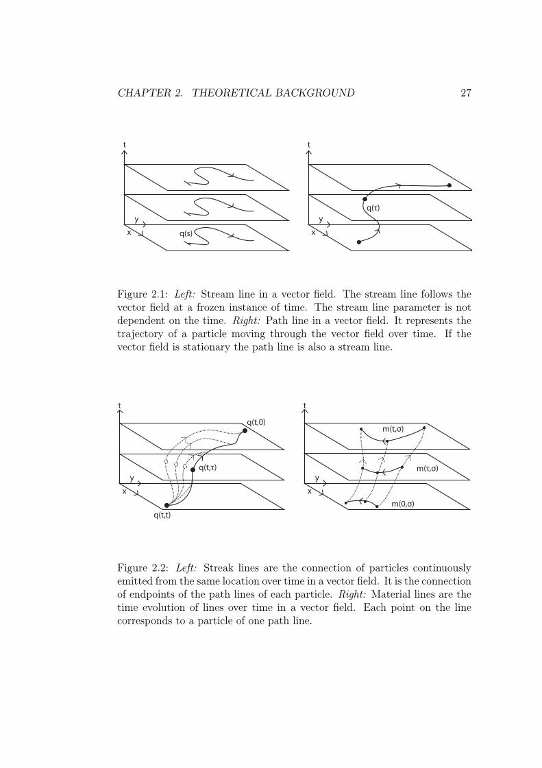
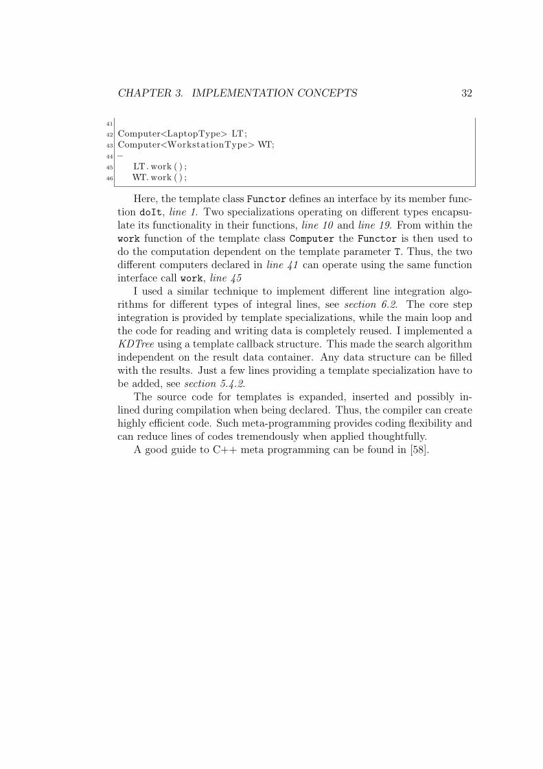
Figure 2.1 and figure 2.2 illustrate these different types of integral linesin a vector field.
In this thesis stream lines were visualized as a pre-stage to geodesics.With v denoting the vector field, stream lines are defined as:
q(s) = v(q(s)) (2.75)
The stream line is a integration line of first order and, thus, one boundarycondition q(0) is required to solve for q(s). The numerical computation ofstreamlines is described in section 6.2 and results are shown in section 7.1and section 7.2.
CHAPTER 2. THEORETICAL BACKGROUND 27
q(τ)
q(s)
t
y
x
t
y
x
Figure 2.1: Left: Stream line in a vector field. The stream line follows thevector field at a frozen instance of time. The stream line parameter is notdependent on the time. Right: Path line in a vector field. It represents thetrajectory of a particle moving through the vector field over time. If thevector field is stationary the path line is also a stream line.
q(t,0)
q(t,τ)
q(t,t)m(0,σ)
m(t,σ)
m(τ,σ)
t t
y
x
y
x
Figure 2.2: Left: Streak lines are the connection of particles continuouslyemitted from the same location over time in a vector field. It is the connectionof endpoints of the path lines of each particle. Right: Material lines are thetime evolution of lines over time in a vector field. Each point on the linecorresponds to a particle of one path line.

CHAPTER 2. THEORETICAL BACKGROUND 28
2.4 Medical Imaging
An application where tensor fields are used stems from medicine. The tech-nology developed in magnetic resonance imaging (MRI) allows to capture thediffusion of hydrogen in human tissue. The resulting tensor fields describethe speed of diffusion in all spatial directions.
The aim of analyzing the anisotropic diffusion is to identify different kindsof brain matters, such as white matter (elongated neurons) which has a highdirectionality in contrast to grey matter (glial cells) which has very littledirectionality.
As stated in [9], tumor regions are dominated by grey matter and thusare regions with low directionality. Tensor field visualization can be used toreveal such regions.
Finding accurate and robust visualization techniques could play an im-portant role in diagnostics of brain tumor diseases using MRI scans. Earlyand precise diagnostic and correct treatment is of great importance to pos-sibly increase the survival rate which, at the moment, is of about 30% only,see [9].
Mathematically the anisotropic diffusion is described by a scalar densityfunction Φ(x, t), e.g. the time-dependent concentration of water molecules:
∂Φ(x, t)
∂t= ∇ ·D[∇Φ(x, t)] (2.76)
Here, D is called the flux and is a function of the concentration gradient∇Φ(x, t). The flux D(v) can be expanded into a Taylor series in the Euclideanchart xµ with chart-functions xi = ei:
D(v) = Di(v)ei =
(Di(0) +Di,j(0)vj +
1
2Dij,k(0)vjvk + ...
)ei (2.77)
The constant flux Di(0) vanishes in equation (2.76) and the second term,the Di,j(0) is a tensor of rank two. The tensor is symmetric and positivedefinite, since particles move forward only (Di,j(0)vj > 0). Di,j(0) is calledthe diffusion tensor.
The diffusion tensor is comparable to the metric tensor in general rel-ativity, see equation (2.29), which is also symmetric and positive definite.The geodesic equation (2.53) can be utilized, exchanging the metric with thediffusion tensor, to compute geodesics in the diffusion field.
The geodesics then represent lines that follow the extremal diffusionspeed. In section 7.5 such spatial geodesics where computed in a numeri-cal diffusion tensor field stemming from a MRI scan of a human brain.

Chapter 3
Implementation Concepts
Software can be implemented in a many different ways. Especially C++provides a lot of flexibility on how problems can be solved and algorithmscan be implemented.
This chapter shortly describes how C++ template meta programmingcan enhance code re-usability, what problems were encountered utilizing thestandard template library and it introduces a mechanism to equip classeswith interfaces at runtime.
3.1 Type Traits
The introduction of templates to C++ opened a wide range of new pro-gramming concepts. Todd Veldhuizen described how to implement programsevaluated at compile time using template meta programming1, see [59]. Tem-plate meta programming theoretically2 provides a programming language in-side C++ that is Touring complete (see [60]) and executes at compile time.Functional programming techniques can be fully utilized to build templateprograms.
Geoffrey Furnish discusses the pros and cons of using C++ for develop-ment of numerical algorithms, see [31]. According to him, C++ code oftenfails the programming paradigm of high re-usability because of its flexibilityto define data structures and classes. He recognized that exchanging andreusing code is easier, for example, in FORTRAN when only limited datastructures, like predefined arrays, were used. However, one can use the power,flexibility and speed of C++ while still developing highly reusable code. He
1The first meta program was written by Erwin Unruh and presented at a C++ standardcommittee meeting in 1994: http://www.erwin-unruh.de
2Theoretically because of limited compilers, such as limited recursion depths.
29

CHAPTER 3. IMPLEMENTATION CONCEPTS 30
discusses and demonstrates the utilization of template meta programming tocreate numerical algorithms independent on data container types.
Meta programming is based on template specializations. Listing 3.1shows a simple example how a template function and specialization can beused to return different strings dependent on a type.
Listing 3.1: Simple example of using template specialization to createstrings dependent on the template class type T.
1 template<class T> string getTypeStr ing ( )2 3 return ”Unknown” ;4 5
6 class MyType /* . . . */ ;7
8 template<> string getTypeString<MyType>()9
10 return ”MyType” ;11 12
13 /* . . . in the main program . . . */14
15 string a = getTypeString<Foo >() ;16 string b = getTypeString<MyType>() ;17
18 /* . . . */
Line 1 defines the general template function that will be called with anytype not specialized. A specialization of the custom type MyType is shownin line 8. In this example string a will contain "Unknown" and string b
"MyType".The general template definition can be interpreted as a definition of an
interface. It ensures a valid call of the function with any type. When usingtemplate classes or functions in such an interface defining way they are calledType Traits in terms of C++ meta programming.
Type Traits can be used to add functionality to certain class types withoutmodifying the classes’ own definitions. Thus, defined classes implemented inan external library can be equipped with functions in the own code, like de-scribed in section 5.2.2, where functions for converting from and to a string
can be provided for any types by a Type Trait.Functions can be gathered in template classed as well. Member functions
defined in the general template class are then similar to pure virtual functionsin classical object oriented programming.
This mechanism can be applied similar to polymorphism in classical ob-

CHAPTER 3. IMPLEMENTATION CONCEPTS 31
ject oriented programming. The next source code listing,listing 3.2, showsan example. The ”virtual” function is called from within another templateclass dependent on the template class type parameter.
Listing 3.2: Example of gathering encapsulated functionality of differenttypes in a unified interface template class enhancing code re-usability. Anew Computer doing some work can be add by introducing the accordingFunctor template specialization.
1 template <class T>2 struct Functor3 4 void doIt ( )5 6 cout << ”Do what?” << endl ;7 ;8 ;9
10 template <>11 struct Functor<LaptopType>12 13 void doIt ( )14 15 doSomethingLaptopTypeSpeci f ic ( ) ;16 ;17 ;18
19 template <>20 struct Functor<WorkstationType>21 22 void doIt ( )23 24 doSomethingWorkstat ionTypeSpeci f ic ( ) ;25 ;26 ;27
28 template<class T>29 struct Computer30 31 /* . . . */32 void work ( )33 34 /* . . . */35 Functor<T> Operator ;36 Operator . doIt ( ) ;37 38 ;39
40 /* . . . */
CHAPTER 3. IMPLEMENTATION CONCEPTS 32
41
42 Computer<LaptopType> LT;43 Computer<WorkstationType> WT;44 −45 LT. work ( ) ;46 WT. work ( ) ;
Here, the template class Functor defines an interface by its member func-tion doIt, line 1. Two specializations operating on different types encapsu-late its functionality in their functions, line 10 and line 19. From within thework function of the template class Computer the Functor is then used todo the computation dependent on the template parameter T. Thus, the twodifferent computers declared in line 41 can operate using the same functioninterface call work, line 45
I used a similar technique to implement different line integration algo-rithms for different types of integral lines, see section 6.2. The core stepintegration is provided by template specializations, while the main loop andthe code for reading and writing data is completely reused. I implemented aKDTree using a template callback structure. This made the search algorithmindependent on the result data container. Any data structure can be filledwith the results. Just a few lines providing a template specialization have tobe added, see section 5.4.2.
The source code for templates is expanded, inserted and possibly in-lined during compilation when being declared. Thus, the compiler can createhighly efficient code. Such meta-programming provides coding flexibility andcan reduce lines of codes tremendously when applied thoughtfully.
A good guide to C++ meta programming can be found in [58].

CHAPTER 3. IMPLEMENTATION CONCEPTS 33
3.2 STL Encapsulation
Container classes of the standard template library (STL) [52] are utilizedespecially in the Fiber Bundle library, chapter 4. Though, the STL providesa beautiful concept to iterate over its template container classes, these iter-ators fail when classes are implemented over different dynamically linkableobjects, such as dlls. Microsoft operating systems do not allow STL objectsto be passed across library boundaries due to memory allocation issues. Thisprevents their use in programming interfaces, [48].
To overcome this problem the Fiber Bundle library uses its own iteratorclasses based on callbacks and wrapping the STL iteration. Such iteratorsare, for example, used to iterate over Fiber Slices, Fiber Grids or field frag-ments. In all that cases an iterator base class declaring a virtual apply
function is provided. The iterator base class has to be derived and imple-mented and can then be utilized by calling the according iterate function.A simple example on how to iterate over field fragments is given in listing4.3.
3.3 Reference Pointers
Smart pointers are a basic design element in modern C++ software develop-ment. They take care about their memory deallocation themselves. Nativepointers in C++ are not exception save. Smart pointers solve this issue. Ref-erence counting pointers are smart pointers that keep track of the number ofreferences, pointers or handles to a resource. They are a typical approach.
Utilizing reference counting pointers reduces misuses and errors in mem-ory management of the software. They can be implemented using templateprogramming. Operator overloading enables a syntax similar to program-ming with native pointers.
The software libraries described in chapter 4 and chapter 5 are based on amemory core library, MemCore, providing strong and weak reference countingpointers with the following features, see [6]:
1. reference counting: keep objects alive exactly as long as at least onepointer refers to it
2. weak and strong pointers:allow back links and circular references
3. support of the up casting operation, conversion from child class to baseclass (going “up” in the class hierarchy), like it is always possible withnative C++ pointers

CHAPTER 3. IMPLEMENTATION CONCEPTS 34
4. support of the downcasting operation: conversion from base class tochild class (going “down” in the class hierarchy), possibly revealinga NULL pointer, similar to the dynamic cast<> pointer conversion inC++
5. constant objects
6. multiple inheritance
7. thread-safety
A strong pointer will keep an object alive, whereas a weak pointer onlyrecognizes the death of an object. Strong and weak pointers are complement-ing concepts and allow circular references. In this implementation, a strongpointer is a weak pointer via inheritance relationships.
Any class can be enabled for reference counting by deriving from theReferenceBase class:
1 template<class T>2 class MyClass : public MemCore : : ReferenceBase<MyClass<T> >3 4 RefPtr<HerClass<T> > element ;5
6 public :7 MyClass ( RefPtr<HerClass<T> >& elementP )8 : e lement ( elementP ) 9
10 /* . . . */11
12 ;13
14 /* . . . */15 RefPtr< HerClass<int> > herFoo = new HerClass<int >() ;16
17 RefPtr< MyClass<int> > myFoo = new MyClass<int>( herFoo ) ;
A reference pointer object can now be created by using the templateRefPtr<> and the standard new, line 15 and line 17. Objects are efficientlypassed by a reference of a reference pointer, line 7 and line 17.
A RefPtr<> can be checked to be valid similar to a native C++ pointer.This concept is used throughout the implemented software for error checking:
1 RefPtr< MyClass<int> > f oo = someContainer−>getData ( ) ;2
3 i f ( ! f oo )4 5 puts ( ” e r r o r ” ) ;

CHAPTER 3. IMPLEMENTATION CONCEPTS 35
6 return ;7

Chapter 4
Modeling of Scientific Data
Computational methods are used more and more in the scientific world. Hugeamounts of data are produced every day. But as the number of applicationsincreases also the diversity of data handling increases and often not muchcare is taken about data exchange-ability.
Modern research often forces to split huge tasks over several researchers orresearch groups that have to collaborate. Data diversity can be a big burdento overcome and many hours are spent on data conversion and handlinginstead of concentrating on real research problems.
However, there exist concepts that can be used to model any kind ofscientific data transparently, efficiently and sustainable. Using and applyingsuch a data model is of great advantage especially in collaborative researchprojects.
Already in 1989 David M. Butler introduced and suggested the conceptfiber bundles to describe data in a unified way, see[19] and [18].
Inspired by this idea Werner Benger developed the Fiber Bundle libraryfor his needs in visualizations stemming from numerical relativity [6]. Data innumerical relativity tend to be quite complex since they often are formulatedin different coordinate systems on non trivial manifolds such as adaptively re-fining meshes. Data sets tend to be huge, with several hundreds of Terabytesof data produced. Numerical relativity is located on the edge of possibilitiesin super-computing technologies.
With this main application in mind he included information such astopology and coordinate representation in a strong and flexible systematicapproach applicable to likely all data occurring in computational scientificdomains.
36

CHAPTER 4. MODELING OF SCIENTIFIC DATA 37
4.1 Fiber Bundle Data Model
The Fiber Bundle is based on Butler’s fiber bundle concept. Here, data isseparated in base space and in fiber spaces where the base space describesthe topological and geometrical data and the fibers the data on the geometry.The data model captures all the semantics of the data. A vector field is notjust a collection of floating point numbers. Rather, it is an array of tangentialvectors in a coordinate system representation on a certain topology of ageometrical object at a certain time. All this information is systematicallyorganized to handle and also store data. The meta information is capturedin a hierarchical layer approach. The actual data sets are hosted in so calleddata fields, that represent the fibers of the bundle.
The two main goals of the Fiber Bundle approach are [6]:
abstract the geometrical description of spatial objects from their nu-merical representation in a specific coordinate
abstract the physical computation domain from its underlying dis-cretization scheme
This allows to formulate algorithms independent of the underlying gridobjects. The line integration algorithms I developed in this thesis are basi-cally formulated grid independently by utilizing the LocalFromWorldPoint
class, see chapter 5.4. Still some algorithms cannot be formulated in such away.
Also a mapping to the file format F5 exists that is utilized by the FiberBundle library for reading and writing. An isolated C-library provides thisfunctionality. The file format is based on HDF51 which is developed andsupported by the NCSA2 HDF5 group for over a decade now. It is stemmingfrom high performance scientific computing applications and addresses manyneeds regarding fast and parallel data access or sustainable archiving, see[33]. For more in depth information about the Fiber Bundle data model, thelibrary and the F5 file format, see [6], [49] and [8].
I omitted the mathematical definitions of fiber bundles here because theymight discourage and confuse. The concept itself is simple and straightfor-ward. For the sake of completeness, I added the mathematical definitions tothe appendix, see appendix B.
1Hierarchical Data Format Version 52National Center for Supercomputing Applications
CHAPTER 4. MODELING OF SCIENTIFIC DATA 38
Fiber Bundle CFD Simulation Data
Time Slice T=0.0
Grid Computational Grid
Topology Vertices
Coordinates Cartesian3D
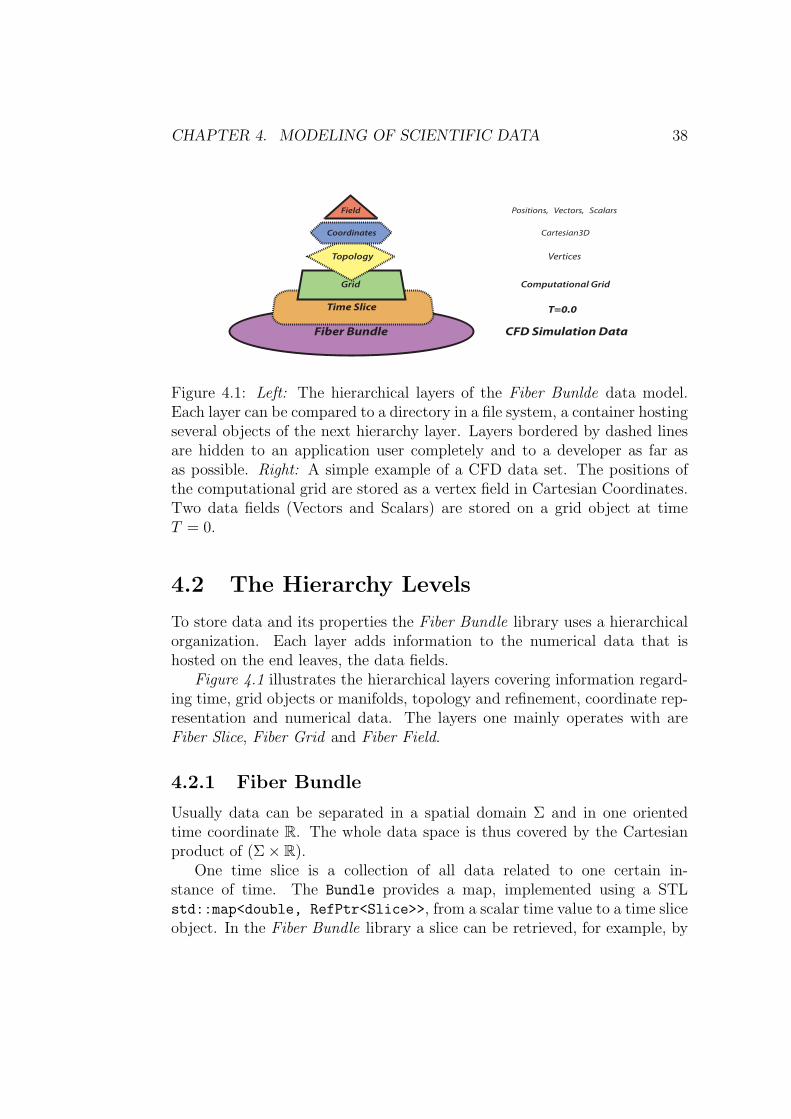
Field Positions, Vectors, Scalars
Figure 4.1: Left: The hierarchical layers of the Fiber Bunlde data model.Each layer can be compared to a directory in a file system, a container hostingseveral objects of the next hierarchy layer. Layers bordered by dashed linesare hidden to an application user completely and to a developer as far asas possible. Right: A simple example of a CFD data set. The positions ofthe computational grid are stored as a vertex field in Cartesian Coordinates.Two data fields (Vectors and Scalars) are stored on a grid object at timeT = 0.
4.2 The Hierarchy Levels
To store data and its properties the Fiber Bundle library uses a hierarchicalorganization. Each layer adds information to the numerical data that ishosted on the end leaves, the data fields.
Figure 4.1 illustrates the hierarchical layers covering information regard-ing time, grid objects or manifolds, topology and refinement, coordinate rep-resentation and numerical data. The layers one mainly operates with areFiber Slice, Fiber Grid and Fiber Field.
4.2.1 Fiber Bundle
Usually data can be separated in a spatial domain Σ and in one orientedtime coordinate R. The whole data space is thus covered by the Cartesianproduct of (Σ× R).
One time slice is a collection of all data related to one certain in-stance of time. The Bundle provides a map, implemented using a STLstd::map<double, RefPtr<Slice>>, from a scalar time value to a time sliceobject. In the Fiber Bundle library a slice can be retrieved, for example, by

CHAPTER 4. MODELING OF SCIENTIFIC DATA 39
Σ
T
Figure 4.2: The collection of all time slices form a Fiber Bundle.
using the () operator of the Bundle class:
RefPtr<Slice> mySlice = myBundle( 0.553 );
Also, the [] operator can be used for access. In that case a new time slicewill be created automatically when no slice at the given time is found.
The Bundle class provides a number of functions and convenient func-tions, for example, to retrieve the next and previous Fiber Slice or to extracta Fiber Grid object of the next or previous time slice.
In contrast to common praxis in many simulations floating point valuesare used to identify time slices instead of integer time steps. Float valuescapture time in a more natural way and allow to store, for example, datasetsstemming from different time discretization in one bundle. This would bedifficult if datasets are accessed by integer time steps but having differentabsolute time resolutions.
Generally, a slice does not need be time but could be a different float-ing point parameter describing something else. Even slicing using multipleparameters could be of interest, but is not yet supported by the library.
Figure 4.2 illustrates a physical space parameterized by a oriented timevalue. All time slices are collected in one bundle.
4.2.2 Fiber Slice
A Slice is a collection of geometrical objects called Fiber Grid objects. Theyare identified by a name. Thus, a slice provides a map of a string to a gridobject.
Again, the () or [] operator is utilized to extract or create a grid object:
RefPtr<Grid> myGrid = mySlice("myName");
The slice provides an GridIterator that can be used to iterate over all ora subset of grid objects of a time slice. To utilize an iterator a GridIterator
CHAPTER 4. MODELING OF SCIENTIFIC DATA 40
T=0.0
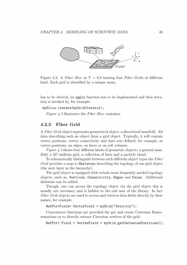
Figure 4.3: A Fiber Slice at T = 0.0 hosting four Fiber Grids of differentkind. Each grid is identified by a unique name.
has to be derived, its apply function has to be implemented and then itera-tion is invoked by, for example:
mySlice.iterate(myGridIterator);
Figure 4.3 illustrates the Fiber Slice container.
4.2.3 Fiber Grid
A Fiber Grid object represents geometrical object, a discretized manifold. Alldata describing such an object form a grid object. Typically, it will containvertex positions, vertex connectivity and data sets defined, for example, atvertex positions, on edges, on faces or on cell volumes.
Figure 4.3 shows four different kinds of geometric objects: a general man-ifold, a 3D uniform grid, a collection of lines and a particle cloud.
To schematically distinguish between such different object types the FiberGrid provides a map to Skeletons describing the topology of one grid object(the next layer in the hierarchy).
The grid object is equipped with certain most frequently needed topologyobjects, such as, Vertices, Connectivity, Edges and Faces. Additionalskeletons can be added.
Though, one can access the topology object via the grid object this isusually not necessary and is hidden to the end user of the library. In factFiber Grid objects are used to access and retrieve data fields directly by theirnames, for example:
RefPtr<Field> VectorField = myGrid("Velocity");
Convenience functions are provided the get and create Cartesian Repre-sentations or to directly extract Cartesian vertices of the grid:
RefPtr< Field > VertexField = myGrid.getCartesianPositions();

CHAPTER 4. MODELING OF SCIENTIFIC DATA 41
Figure 4.4: Dimensionality of some example topological objects. From leftto right: Vertex: 0, Edge: 1, Quad-Face: 2, Cubic-Cell: 3.
4.2.4 Fiber Topology
The object describing the topology of the data is called a Skeleton in theFiber Bundle library. It holds the neighborhood information and it is char-acterized by three integer numbers: the dimensionality, the index depthand the refinement level.
The neighborhood information is in the most general case stored as a listof neighbors of one spatial elements to the others as a list of indices. In manycases the neighborhood can be expressed procedurally and no explicit datahas to be stored, as, for example, neighbors of vertices of a uniform grid.
The dimensionality describes the dimensions that the data, stored in thedata fields, is associated with. A dimensionality of 0 represents a vertex, 1represents a line or an egde, 2 a surface or polygon, 3 a volume or cell and4 a hyper-volume, and so forth. Figure 4.4 illustrates the dimensionality upto 3.
If, for example, scalar values are stored on 3D cell volumes the scalardata field would be nested in a Skeleton of dimensionality 3. The data fielddescribing the vertices of the cell corners would be stored in a Skeleton ofdimensionality 0.
Index depth describes how many “dereferencing” or “lookup” operationsare necessary to get “down” to a vertex of the geometrical object. An edge,for example, can be defined as a pair of two vertices (or pair of indices ofvertices), resulting in an index depth on 1. A path can be defined based onthese edges. Now, to get “down” to the vertex level one has to first lookupthe edge and then lookup the vertex. Thus, a path, defined via edges has anindex depth of 2. The following table illustrates several possible values forskeleton characteristics by example (taken from [6]):
CHAPTER 4. MODELING OF SCIENTIFIC DATA 42
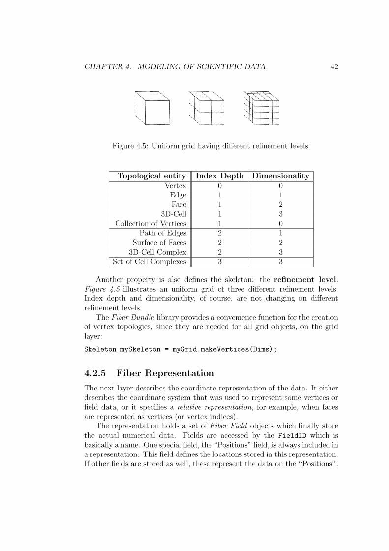
Figure 4.5: Uniform grid having different refinement levels.
Topological entity Index Depth DimensionalityVertex 0 0
Edge 1 1Face 1 2
3D-Cell 1 3Collection of Vertices 1 0
Path of Edges 2 1Surface of Faces 2 2
3D-Cell Complex 2 3Set of Cell Complexes 3 3
Another property is also defines the skeleton: the refinement level.Figure 4.5 illustrates an uniform grid of three different refinement levels.Index depth and dimensionality, of course, are not changing on differentrefinement levels.
The Fiber Bundle library provides a convenience function for the creationof vertex topologies, since they are needed for all grid objects, on the gridlayer:
Skeleton mySkeleton = myGrid.makeVertices(Dims);
4.2.5 Fiber Representation
The next layer describes the coordinate representation of the data. It eitherdescribes the coordinate system that was used to represent some vertices orfield data, or it specifies a relative representation, for example, when facesare represented as vertices (or vertex indices).
The representation holds a set of Fiber Field objects which finally storethe actual numerical data. Fields are accessed by the FieldID which isbasically a name. One special field, the “Positions” field, is always included ina representation. This field defines the locations stored in this representation.If other fields are stored as well, these represent the data on the “Positions”.
CHAPTER 4. MODELING OF SCIENTIFIC DATA 43
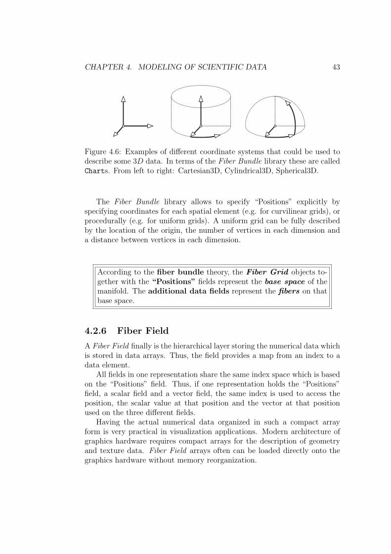
Figure 4.6: Examples of different coordinate systems that could be used todescribe some 3D data. In terms of the Fiber Bundle library these are calledCharts. From left to right: Cartesian3D, Cylindrical3D, Spherical3D.
The Fiber Bundle library allows to specify “Positions” explicitly byspecifying coordinates for each spatial element (e.g. for curvilinear grids), orprocedurally (e.g. for uniform grids). A uniform grid can be fully describedby the location of the origin, the number of vertices in each dimension anda distance between vertices in each dimension.
According to the fiber bundle theory, the Fiber Grid objects to-gether with the “Positions” fields represent the base space of themanifold. The additional data fields represent the fibers on thatbase space.
4.2.6 Fiber Field
A Fiber Field finally is the hierarchical layer storing the numerical data whichis stored in data arrays. Thus, the field provides a map from an index to adata element.
All fields in one representation share the same index space which is basedon the “Positions” field. Thus, if one representation holds the “Positions”field, a scalar field and a vector field, the same index is used to access theposition, the scalar value at that position and the vector at that positionused on the three different fields.
Having the actual numerical data organized in such a compact arrayform is very practical in visualization applications. Modern architecture ofgraphics hardware requires compact arrays for the description of geometryand texture data. Fiber Field arrays often can be loaded directly onto thegraphics hardware without memory reorganization.
CHAPTER 4. MODELING OF SCIENTIFIC DATA 44
0 1 2
0
0
1
1
2
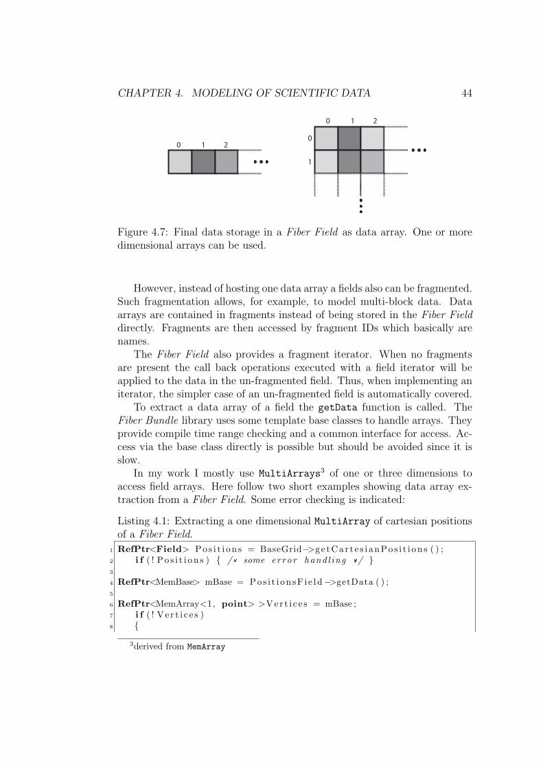
Figure 4.7: Final data storage in a Fiber Field as data array. One or moredimensional arrays can be used.
However, instead of hosting one data array a fields also can be fragmented.Such fragmentation allows, for example, to model multi-block data. Dataarrays are contained in fragments instead of being stored in the Fiber Fielddirectly. Fragments are then accessed by fragment IDs which basically arenames.
The Fiber Field also provides a fragment iterator. When no fragmentsare present the call back operations executed with a field iterator will beapplied to the data in the un-fragmented field. Thus, when implementing aniterator, the simpler case of an un-fragmented field is automatically covered.
To extract a data array of a field the getData function is called. TheFiber Bundle library uses some template base classes to handle arrays. Theyprovide compile time range checking and a common interface for access. Ac-cess via the base class directly is possible but should be avoided since it isslow.
In my work I mostly use MultiArrays3 of one or three dimensions toaccess field arrays. Here follow two short examples showing data array ex-traction from a Fiber Field. Some error checking is indicated:
Listing 4.1: Extracting a one dimensional MultiArray of cartesian positionsof a Fiber Field.
1 RefPtr<Field> P o s i t i o n s = BaseGrid−>g e t C a r t e s i a n P o s i t i o n s ( ) ;2 i f ( ! P o s i t i o n s ) /* some error hand l ing */ 3
4 RefPtr<MemBase> mBase = P o s i t i o n s F i e l d−>getData ( ) ;5
6 RefPtr<MemArray<1, point> >V e r t i c e s = mBase ;7 i f ( ! V e r t i c e s )8
3derived from MemArray
CHAPTER 4. MODELING OF SCIENTIFIC DATA 45
9 puts ( ” Error : MemArray<1, point> i s incompat ib le ! Type i s : ” ) ;10 mBase . speak ( ”some text ” ) ;11 return ;12 13
14 MultiArray<1, point>&BaseCrds = *BaseVert i ce s ;15
16 MultiIndex<1> mi ;17 mi=0;18
19 point myPoint = BaseCrds [ mi ] ;
First the field is extracted from the underlying grid object by using a conve-nience function, line 1. Then data is retrieved into a array class MemArray
of dimension 1 and type of points. When no field or no data can be re-trieved the according reference pointer is null and can be used for errorchecking. When the MemBase is retrieved first it can be used to get infor-mation about the data object in case of an error, lne10. Finally, a referenceof MultiArray is instantiated downcasting the dereferenced MemArray, line14. The MultiArray can be accessed using a one dimensional MultiIndexefficiently.
Here follows an example that shows the extraction of a three dimensionalvector array from a fragmented field by fragment name. Error checking isomitted:
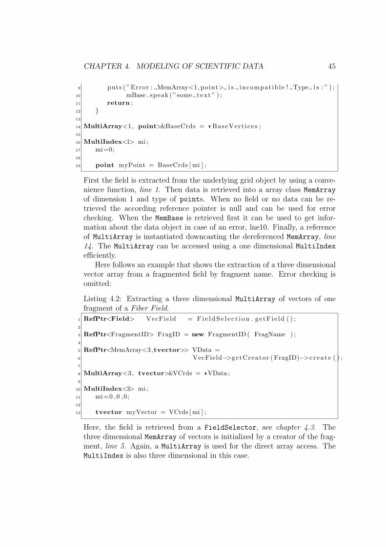
Listing 4.2: Extracting a three dimensional MultiArray of vectors of onefragment of a Fiber Field.
1 RefPtr<Field> VecField = F i e l d S e l e c t i o n . g e t F i e l d ( ) ;2
3 RefPtr<FragmentID> FragID = new FragmentID ( FragName ) ;4
5 RefPtr<MemArray<3,tvector>> VData =6 VecField−>getCreator ( FragID)−>c r e a t e ( ) ;7
8 MultiArray<3, tvector>&VCrds = *VData ;9
10 MultiIndex<3> mi ;11 mi=0 ,0 ,0 ;12
13 tvector myVector = VCrds [ mi ] ;
Here, the field is retrieved from a FieldSelector, see chapter 4.3. Thethree dimensional MemArray of vectors is initialized by a creator of the frag-ment, line 5. Again, a MultiArray is used for the direct array access. TheMultiIndex is also three dimensional in this case.
CHAPTER 4. MODELING OF SCIENTIFIC DATA 46
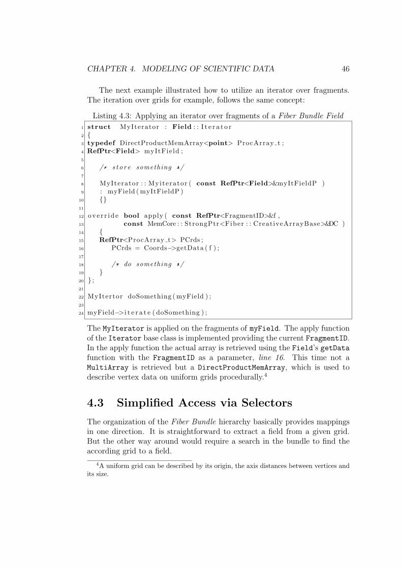
The next example illustrated how to utilize an iterator over fragments.The iteration over grids for example, follows the same concept:
Listing 4.3: Applying an iterator over fragments of a Fiber Bundle Field
1 struct MyIterator : Field : : I t e r a t o r2 3 typedef DirectProductMemArray<point> ProcArray t ;4 RefPtr<Field> myItFie ld ;5
6 /* s t o r e something */7
8 MyIterator : : Myiterator ( const RefPtr<Field>&myItFieldP )9 : myField ( myItFieldP )
10 11
12 o v e r r i d e bool apply ( const RefPtr<FragmentID>&f ,13 const MemCore : : StrongPtr<Fiber : : CreativeArrayBase>&DC )14 15 RefPtr<ProcArray t> PCrds ;16 PCrds = Coords−>getData ( f ) ;17
18 /* do something */19 20 ;21
22 MyItertor doSomething ( myField ) ;23
24 myField−>i t e r a t e ( doSomething ) ;
The MyIterator is applied on the fragments of myField. The apply functionof the Iterator base class is implemented providing the current FragmentID.In the apply function the actual array is retrieved using the Field’s getDatafunction with the FragmentID as a parameter, line 16. This time not aMultiArray is retrieved but a DirectProductMemArray, which is used todescribe vertex data on uniform grids procedurally.4
4.3 Simplified Access via Selectors
The organization of the Fiber Bundle hierarchy basically provides mappingsin one direction. It is straightforward to extract a field from a given grid.But the other way around would require a search in the bundle to find theaccording grid to a field.
4A uniform grid can be described by its origin, the axis distances between vertices andits size.

CHAPTER 4. MODELING OF SCIENTIFIC DATA 47
In the Vish visualization environment, see chapter 5, that heavily uti-lized the Fiber Bundle library sometimes fiber accesses were difficult. Se-lector classes were introduced for convenience that would store much morerelated information. Two selector classes are available: a GridSelector anda FieldSelector, which is derived from the former.
The GridSelector class holds the name of the selected grid and a handleto the bundle it is hosted in. It provides functions to extract grid objectsthat are closest to a given time and functions that extract grid objects nextor previous to a given time. Having a GridSelector available the grid at acurrent time t can be extracted via:
RefPtr<Grid> myGrid = myGridSelector->findMostRecentGrid( t );
The next or previous grid can be extracted by:
RefPtr<Grid> myGrid= myGridSelector->findNext( t );
RefPtr<Grid> myGrid= myGridSelector->findPrev( t );
Since the FieldSelector is derived from GridSelector it pro-vides the functionality described above and additionally allows to ex-tract the selected field, the grid and the time slice carrying the field:
RefPtr<Field> myField = myFieldSelector->getField()
RefPtr<Grid> myGrid = myFieldSelector->getGrid()
RefPtr<Slice> mySlice = myFieldSelector->getSlice()
Another convenience function returns the “Positions” field accordingto the selected data field, if they are given in Cartesian representation:
RefPtr<Field> myPositions = getCartesianPositions();
More convenience functions are available and can be found in the docu-mentation, see chapter 5.1.2.
The selector classes are now used as data handles (for example as mod-ule parameters) in the Vish environment and simplify the fiber data accesstremendously.
4.4 Data Examples
Three examples of how data is laid out in the Fiber Bundle model are shownin this section. The examples describe most of the data I used in the thesis:
a uniform grid hosting vector, scalar or tensor field data

CHAPTER 4. MODELING OF SCIENTIFIC DATA 48
Fib
er B
un
dle
T=0.0 UniformGrid Vertices Cartesian3D Positions
Velocity
T=0.3 UniformGrid Vertices Cartesian3D Positions
Velocity
T=... UniformGrid Vertices Cartesian3D Positions
Velocity
Figure 4.8: Structure of Fiber Bundle layers of the uniform grid hosting avector field for velocity, as it is used to describe the Couette flow field inchapter 7.1. Here, the light red color of the “Velocity” data field indicatesthe fiber on the manifold. The two data fields (red) are contained in theCartesion3D representation.
a curvilinear multi-block grid hosting vector and scalar data
a grid that describes lines with additional data stored on them
4.4.1 Uniform, procedural
Many data are provided on a uniform hexahedral procedural grid formulatedin Cartesian coordinates. The 3D vector field of the Couette flow applicationand the metric tensor fields are created by Analytic Creators that samplean uniform grid based on some formula. Data is sampled on demand bythe creator when it is requested. The diffusion tensor field used in the MRIapplication is read from numerical data, but is also hosted by a uniformprocedural grid, see chapter 7.
Figure 4.8 shows the hierarchical layout of the vector field used in theCouette flow application, see chapter 7.1. It provides a vector field on auniform grid. The original stationary flow is scaled over time, thus, severaltime slices are stored in the bundle. In this application all field data iscomputed on demand, stored and kept in the bundle, just before data isaccessed the first time.
The uniform grid (the base space) itself does not change over time. TheFiber Bundle library will just reuse the same grid object for all time steps in

CHAPTER 4. MODELING OF SCIENTIFIC DATA 49
Fib
er B
un
dle T=0.0 Curvilinear
MultiblockVertices Cartesian3D Positions
Velocity
Pressure
Figure 4.9: Structure of Fiber Bundle layers of the curvilinear multi-blockgrid hosting a vector field for velocity and a scalar field for pressure, as itis used to describe data for the stirtank in chapter 7.2. Again, the light redcolors illustrate the fibers on the manifold sharing the index space of the“Position”.
that case, though this is not visible in the data layout. The only componentthat is changing over time is the vector field describing velocity (the fiber).
The data layout itself does not differ between grids given procedurally orexplicitly. The difference is located in the array data structure used to vertex“Positions” data. As described above a DirectProductMemArray is used tostore procedural coordinates. The coordinate array of a procedural uniformgrid can be extracted using the getData() function of a field, for example:
1 typedef DirectProductMemArray<point> ProcArray t ;2 RefPtr<ProcArray t> ProcCrds = myPosit ionFie ld−>getData ( ) ;
4.4.2 Multiblock, Curvilinear
The data from the stir tank application, see chapter 7.2, is given in curvilinearmulti-block data. Coordinates of the grid object are given explicitly and areseparated over multiple blocks of coordinates. The coordinates are given ona hexahedral grid.
The Fiber Bundle data model captures the multi-block organization bystoring its field as fragmented fields. Each fragment refers to one multi-block.
Figure 4.9 illustrated the hierarchical layout. The differences to the uni-form grid example are, that data fields are stored using MultiArrays, forexplicit coordinates, and that data fields are fragmented. The data set holdsa vector field for velocity and a scalar field for pressure, stored as fibers onthe grid object. Besides the index space now also the space of fragment IDsis shared among the fibers hosted on the vertex “Positions”.
Fields must be accessed using fragment IDs or via fragment iterators asdescribed above.

CHAPTER 4. MODELING OF SCIENTIFIC DATA 50
Fib
er B
un
dle
T=0.0 Streamlines Vertices Cartesian3D Positions
Directions
TangentialVectorFieldName
Magnitude
FieldData
LocalCoords
LineEdges EdgesAsVertices Positions
SourceFragments VerticesAsFragment Positions
Figure 4.10: Structure of Fiber Bundle layers of the grid describing computedintegral lines as they are used throughout all applications chapters. The lightred colors illustrate the fibers on the manifold sharing the index space of the”Position”. Here, data fields are stored on the vertices of the lines. The edgesof the lines are stored in its own topology using a relative representation onthe Vertices, thus, using vertex indices to describe edges. An additionaltopology SourceFragments stores multi-block IDs relatively to the vertices.The fiber field TangentialVectorFieldName is an alias to Directions usedas convention for rendering modules in Vish.
4.4.3 Lines
The lines stemming from the integration, see chapter 6, are also stored usingthe Fiber Bundle data model.
This example shows the application of relative representations. First,the lines store information “what make them lines”. Vertex positions arestored in the topology Vertices. Now, the LineEdge topology (indexdepth 1, dimensionality 1) defines edges by using the relative representationEdgesAsVertices. Thus, vertex indices are used to define edges. Tangen-tial direction vectors are computed during integration and are stored in thedata field Directions. To provide compatibility to line grids in the Vishenvironment an alias TangentialVectorFieldName is provided, as well.
Next, data related to the data field that is being integrated is stored.The data field value at the vertex position is stored in the fiber FieldData.In case of streamlines this is the velocity vector and in case of geodesicsthis is the metric tensor. A norm of this object is stored in the scalar field

CHAPTER 4. MODELING OF SCIENTIFIC DATA 51
Magnitude.Finally, data that will speed up sampling of any other field on the line
grid is stored, i.e. interpolation weights. This information includes the localindex coordinates of a vertex, see chapter 5.4, and the IDs of the multi-block, a vertex is contained in. Local coordinates are stored as a fiber inthe vertex topology and fragments (or better fragment IDs) are stored ona different topology (index depth 1 and dimensionality 3) using a relativerepresentation on the vertices.
Example code illustrating data storage using the Fiber Bundle library isgiven in chapter 6.2.
Chapter 5
Vish - The Vis(h)ualizationEnvironment
Vish is the visualization application of choice for this thesis. It it a very mod-ular, flexible and fast framework especially build for scientific visualizationcreated mainly by Werner Benger. It provides the programmer with a lotof functionality addressing problems especially faced when doing scientificvisualization, such as, handling large data sets and memory management.It provides an automatically generated GUI, 3D rendering with camera andtime navigation, hierarchical caching, mathematical functionality and a num-ber of standard modules for analyzing datasets.
It is meant to enable the developer to focus on visualization algorithmsand not spending his and her time on basic tasks like GUI programming orreading and writing data files. This comes, of course, with the cost of learningand understanding some concepts of the visualization environment. It followsa systematic approach using strong theoretical concepts in the background.This helps to create overall more reusable code. These concepts are:
Topology
Differential Geometry
Geometric Algebra
This chapter should help to overcome this hurdle and will give a quickstart. Since most of this information is available already on some web docu-mentation or tutorial examples it is kept short and will give some referencesto further reading. While basics are described here shortly, more in-depthexamples will be explained by describing parts of the source code written forcomputing the geodesics in the following in chapter 6. Also, see [11] for moredescriptions of concepts behind Vish.
52
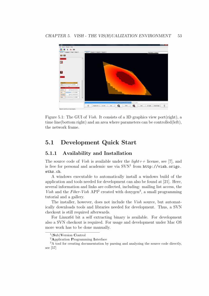
CHAPTER 5. VISH - THE VIS(H)UALIZATION ENVIRONMENT 53
Figure 5.1: The GUI of Vish. It consists of a 3D graphics view port(right), atime line(bottom right) and an area where parameters can be controlled(left),the network frame.
5.1 Development Quick Start
5.1.1 Availability and Installation
The source code of Vish is available under the light++ license, see [7], andis free for personal and academic use via SVN1 from http://vish.origo.
ethz.ch.A windows executable to automatically install a windows build of the
application and tools needed for development can also be found at [21]. Here,several information and links are collected, including: mailing list access, theVish and the Fiber-Vish API2 created with doxygen3, a small programmingtutorial and a gallery.
The installer, however, does not include the Vish source, but automat-ically downloads tools and libraries needed for development. Thus, a SVNcheckout is still required afterwards.
For Linux64 bit a self extracting binary is available. For developmentalso a SVN checkout is required. For usage and development under Mac OSmore work has to be done manually.
1(Sub)Version Control2Application Programming Interface3A tool for creating documentation by parsing and analyzing the source code directly,
see [57]

CHAPTER 5. VISH - THE VIS(H)UALIZATION ENVIRONMENT 54
Dependencies on external libraries are kept as minimal as possible. As ofnow, the following external libraries are required:
QT, a cross platform GUI library, see [45]
GNU Bison and Flex, a GNU parser generator and lexer, from [30]
GNU FreeType, a GNU font library
HDF5, a hierarchical file format, see [33]
Earlier the HDF5 file format library had to be downloaded manually but itwas added to the Vish SVN repository, lately.
To get access to the SVN one must join the vish group and, thus, mustbe added to the group to get full permissions.
Installation instructions can be found at origao, see [64], underdevelopment. When using windows it is best to install using the installerprovided at [21] and to install all libraries or programs into the standard di-rectory that is suggested by each installer. Otherwise it might get necessaryto modify some Makefiles during compilation.
5.1.2 Source Code Organization and Naming Conven-tions
Vish follows an own naming convention through directory, file and classnames. The Vish kernel is called the ocean which represents the environmentinhabiting classified beings.
The ocean has interfaces to four big code areas which are connected tothe kernel only:
GUI
Script
Graphics
Data I/O
The preferred components are the Qt library for the GUI, a simple scriptinterpreter, OpenGL for Graphics and HDF5 for Data I/O. They can beexchanged by using the provided interfaces.
The more high level the code in the kernel gets the higher levelis the classification of the being living in the ocean. Starting fromthe $VISH/ocean/plankton library and becoming more complex via e.g.
CHAPTER 5. VISH - THE VIS(H)UALIZATION ENVIRONMENT 55
$VISH/ocean/shrimp to $VISH/ocean/eagle, which for example providesmathematical, algebraic classes. Typically a being consists of several APIsource files. If there are concrete Vish modules, section 5.2, implementedbased on the contained source files the directory will contain a directorycalled egg hosting these implementations.
A complex being is the $VISH/fish/fiber library. This is the Fiber Bun-dle library as described in chapter 4, which is independent. All source codedependent on the $VISH/ocean and the $VISH/fish/fiber library are gath-ered in the $VISH/fish/lakeview directory. Here, almost all Vish Modulescan be found.
When developing a new Vish Module without extending the Vish kernelthis most likely the directory where the source code will be placed.
Both, the $VISH/ocean and the $VISH/fish library use the$VISH/memcore library which provides basis classes for memory manage-ment, such as, template classes for reference pointers. Native pointers areavoided in source code and strong and weak reference pointers are preferred,section 3.3. This reduces programming errors due to allocation and freeingof memory.
The Vish coding style usually intends that code is separated in header(*.hpp) and implementation(*.cpp) files. Usually every class is placed inan own file which has the same name as the class. For example, an classimplementation called RandomPointDistribution is placed in the file or filesRandomPointsDistribution.cpp and/or RandomPointDistribution.hpp.
Classes or source files are kept short. In the best case, files will have lessthan 300 lines of code. Up to 800 is considered as acceptable but having morelines of code should give the programmer a hint for refactoring and clearerorganization the code. Maybe some functionality can be gathered and madebetter reusable in another header file.
Experimental test or source code should be placed in$VISH/modules/examples where some examples of implementations ofdifferent kinds can be found.
While working into the software environments I created a quick starttutorial which starts from very a simple example. More complex source codeexamples demonstrate how to use OpenGL and the Fiber Bundle library.The tutorial can be found in the $VISH/tutorial directory.
All documentation is located in $VISH/doc but has to be created manu-ally. There are different parts of the documentation that have to be createdeach. For creation of the Vish documentation invoke make doc in the $VISH/parent directory. For creation of the Fiber Vish (Fish) documentation invokemake doc in the $VISH/fish directory. Make doc in the $VISH/tutorial di-rectory creates the documentation for the tutorial. These documentation can

CHAPTER 5. VISH - THE VIS(H)UALIZATION ENVIRONMENT 56
also be found online at [21].The directory $VISH/data is used to place f5 data files, see [49], or vis
script files, section 5.2.4
5.1.3 Make Files and Compilation
The Vish project uses a make file system. The basis make file configurationsfor different platforms, like Linux 64, Windows 32, etc. are located in the$VISH/make directory. Internally the uname command is used to differentiatebetween platforms and the returned string of the command is concatenatedto the arch- prefix.
Each directory containing source files contains a file Makefile specifyingthe following:The name of the dynamically linkable object is defined by, for exam-ple, VISH=fishcephalus. During compilation a file fishcephalus.dll orfishcephalus.so is created and placed in the $VISH/bin/$arch directorycontaining the compiled code of the source of this directory.Script files can be copied to the $VISH/data directory by specifying VIS=
followed by a list of *.vis files separated by a whitespace.All libraries that are necessary for linking have to be specified by LIBS= fol-lowed by strings ’-l’ concatenated with the name of the library separated bya whitespace.If OBJS= is specified the following list of .cpp files are used for compilation.If not specified all .cpp files in the directory are compiled.The Makefile ends with include $(VPATH)../GNUmakefile.rules. For amore detailed description of the make file system, see the documentationlocated at $VISH/make/doc. A typical Makefile is shown in listing 5.1.
Listing 5.1: Typical Vish Makefile. The example shows a simplified versionof the Makefile found in the $VISH/fish/lakeview/cephalus directory
1 VISH=f i s h c e p h a l u s2
3 VIS=GridSubtractor . v i s GridAdder . v i s GridConvolver . v i s . . .4
5 LIBS=−lbundle − l f i b e r b a s e o p − l f i b e r o p −l shr imp −l p lankton6 $ (FIBERLIBS) −lmemcore −lm − l f i s h b o n e $ (OCEAN)7
8 i n c lude $ (VPATH) . . / GNUmakefile . r u l e s
Compilation of the source is done using a gcc4 compiler in the accordingsystem by invoking make in the parent Vish directory $VISH/. Parts of the
4Version 3.4.2 or newer.
CHAPTER 5. VISH - THE VIS(H)UALIZATION ENVIRONMENT 57
Vish environment can be compiled by invoking make in the appropriate sub-directory or by providing the directory name after make -C.To compile in debug mode use make Make CFG=Debug and to compile opti-mized use make MAKE CFG=Optimize.Make libclean deletes all precompiled object files located in the $VISH/lib
directory and make clean does a complete cleanup in the current directory.
5.2 Scene Network
To solve an entire visualization task Vish breaks this task into small pieces ofwork. An entity processing a small piece of task is called a module. Modulesare connected by a directed graph or network. The graph can also allowscycles. Information is passed in two steps through the graph. A controls flowdecides what has to be updated and the data flow transports the information.
It is a common approach to break tasks into such building blocks ingraphic applications. Atomic tasks can be combined in many different waysto solve complex tasks making this a very flexible approach.
Famous examples of graphics applications that successfully use a networkscheme are Autodesk Maya (a professional 3D application used in movie pro-ductions, see [3]), Eyon Fusion (a nonlinear compositing application used inmovie productions, see [27]), Avizo, the former Amira (a scientific visual-ization toolkit, see [62]) and OpenDX (a scientific visualization toolkit, see[46]).
However, there are different schemes of how data is flowing through thenetwork or how recomputing of modules is controlled. Vish uses a data pullscheme. Thus, the end or sink nodes of the network, which typically aremodules responsible for rendering, notify the connected upstream modulesthat they need to provide up to date data. This request is forwarded tothe next upstream connected modules and finally all involved modules areupdated or recomputed from source to sink.
So, sink modules pull from the sources and updates are only done wherethey are really needed. Maya, for example, uses a similar technique, byfirst flagging necessary updates starting from the sink modules, see [55]. Incontrast, Avizo uses a push scheme where data sources push the data throughto the sink nodes.
The following section explains how the existing Vish network capabilitiescan be extended by introducing new modules and new data types for thedata transport. It also introduces data access using the Fiber Bundle libraryand describes how rendering is done. Finally, the script language to storenetworks in text files is presented.

CHAPTER 5. VISH - THE VIS(H)UALIZATION ENVIRONMENT 58
Figure 5.2: Example of a module network shown in the network frame ofVish’s GUI. Modules can be created by the user via a context menu showinga hierarchical list of all modules which appears when clicking on an emptyspace in the network frame, see figure 5.1. When doing a right click onan existing module a context menu appears containing modules that havecompatible input parameters to the output parameter of the right clickedmodule. A created module then is automatically connected.
5.2.1 Modules
Modules are the building block of the Vish network. They are derivedfrom the base class VObject and have to overload the function bool
update(VRequest&R, double precision). The module usually is equippedwith input and output parameters. When a module is requested to update5
it executes the update function and typically recomputes the output param-eters dependent on the input parameters.
An input parameter can be added by declaring the template classTypedSlot< ParameterType > in the derived VObject. In the constructorof the class the parameter is initialized and also properties for a parametercan be set.
In the same way, an output can be added by declaring the template classVOutput< ParameterType >. Initialization and configuration also is done inthe constructor.
Examples of supported parameter types are int, double, Enum,Eagle::PhysicalSpace::point, Eagle::PhysicalSpace::tvector, Eagle::PhysicalSpace::metric33, Eagle::rgba float t. Custom types can beadded, as described in section 5.2.2.
5An internal age parameter is used for that purpose.

CHAPTER 5. VISH - THE VIS(H)UALIZATION ENVIRONMENT 59
To ensure thread save behavior it is forbidden to store data in the moduleby using a typical data type in the module class. Data is always dependenton a context. So, also when accessing input and output parameters this isalways done via the context. The context is provided in the update functionvia the VRequest&R object.
Listing 5.2 shows how to implement a simple Vish module. It has twoinput and one output parameter of type int. In the update function theoutput is computed dependent on the input doing a multiplication. So, themodule just multiplies two integer numbers and outputs its result.
Listing 5.2: Source code example of a simple Vish module. TheMultiPlyInt example class can also be found in the tutorial section at/tutorial/basic/MultiplyInt.cpp
1 #include <ocean / plankton /VCreator . hpp>2 #define o v e r r i d e3
4 using namespace Wizt ;5
6 class Mult ip ly Int : public VObject7 8 TypedSlot<int> IntInParam ;9 TypedSlot<int> M u l t i p l i e r ;
10 VOutput<int> IntOutParam ;11
12 public :13 Mult ip ly Int ( const string & name , int p ,14 const RefPtr< VCreat ionPre ferences > & VP)15 : VObject( name , p , VP )16 , IntInParam ( this , ” i n t i n pu t ” , 0 )17 , M u l t i p l i e r ( this , ” m u l t i p l i e r ” , 2 )18 , IntOutParam ( s e l f ( ) , ” intoutput ” , 1 )19 20 M u l t i p l i e r . s e tProper ty ( ”max” , 8 ) ;21 22
23 o v e r r i d e bool update ( VRequest & R, double p r e c i s i o n )24 25 int x = 0 ;26 int m = 0 ;27
28 IntInParam << R >> x ;29 M u l t i p l i e r << R >> m;30
31 x *= m;32
33 IntOutParam << R << x ;34

CHAPTER 5. VISH - THE VIS(H)UALIZATION ENVIRONMENT 60
Figure 5.3: Example of a module shown on different expert levels. When themodule is displayed in the GUI parameters with a high parameter value arehidden. The expert level that should be shown can be increased by clickingthe + button in the header of the module. This is used to hide parametersfrom the user that are not needed frequently. The expert level increases fromleft to right.
35 return true ;36 37 ;38
39 stat ic Ref< VCreator<Mult ip lyInt , AcceptList<int> > >40 VMult ip lyIntCreator ( ” Tutor i a l / Mul t ip ly Int ” ,41 ObjectQual i ty : :EXPERIMENTAL) ;42
43 VISH DEFAULT INIT
The macro in line 2 is used to label function if they are overloading a purevirtual function. This makes code better readable and understandable andis used throughout the most parts of source code in the Vish environment.Thus, the update function in line 23 is flagged since it is an overridingfunction of VObject.
The module MultiplyInt is derived from VObject making it a Vish net-work module. The module is equipped with one output and two input integerparameters, line 8 to line 10.
The parameters of the constructor, line 13, are just handled to the superclass, see line 15. The TypedSlot< > parameters are initialized by usingthe constructor syntax with the following parameters: this, a string speci-fying the name of the parameter in the GUI and script, the initial value andoptionally a so called expert level.
The body of the constructor is used to set properties of parameters. Here,a maximum value for the Multiplier parameter is set to 8, see line 21.
CHAPTER 5. VISH - THE VIS(H)UALIZATION ENVIRONMENT 61
Finally, the update function is overridden. To get the values of the inputinto local types the context R has to be used. Line 29 and line 30 shows howthis is done using the << operator to read from the context in combinationwith the >> operator to write to the local type. Now, the local types can beused in computations, as in line 32.
The value of a local type is written to the output parameter in a similarfashion by using the >> operator via the context R.
The module itself is ready for use now but a static VCreator object hasto be provided for Vish. It defines what types can be connected to the moduleand specifies a name and place in the GUI context menu for the modulecreation. The first template parameter defines the class that is created, thesecond the a list of compatible input parameter types. The AcceptList< >
template can be nested when more than one type is required. The name ofthe VCreator class is arbitrary but the parameter string is important andspecifies the name of the module in the creation context menu. It is also thestring used to create a module instance in the *.vis script language, section5.2.4. The second parameter sets a category used to filter modules in theGUI menu. Possible values are ObjectQuality: :RECOMMENDED, :MATURE,:DEMO, :BETA, :EXPERIMENTAL, :TEMPORARY and :OUTDATED.
If necessary, data can be stored or cached in the module from one update
call to another by using a provided state object. To add such a state class anested state class has to be defined in the module class and a creator functionhas to be overridden, see listing 5.3.
Listing 5.3: Adding a state class to remember data from previous update
calls.
1 class Mult ip ly Int : public VObject2 , public StatusIndicator3 4 /* . . . */5 struct MyState : State6 7 int remember value ;8 ;9
10 o v e r r i d e RefPtr<State> newState ( ) const11 12 return new MyState ( ) ;13 14 /* . . . */15 o v e r r i d e bool update ( VRequest & R, double p r e c i s i o n )16 17 /* . . . */18 RefPtr<MyState> s t a t e = myState (R) ;

CHAPTER 5. VISH - THE VIS(H)UALIZATION ENVIRONMENT 62
19
20 s ta te−>remember value = x ;21
22 s e t S t a t u s I n f o (R, ”Computation done ! ” ) ;23 /* . . . */24 25 ;
Now, MyState can be used to store data. The simplified example makesno real sense here. It just shows the correct procedure to add and access datavia a state object. Also, other possibilities for caching data are provided,section 5.3.
A number of super classes for multiple derivation are provided forVObjects. Features such as printing text messages in the GUI can be addedby deriving from the StatusIndicator class, see listing 5.3. Now, the func-tions setStatusError and setStatusInfo can be used in the update func-tion for printing strings, see line 22.
5.2.2 Data Transport and Access
Creating new Parameter Types
New valid parameter types for the TypedSlot< > template can be defined.Firstly, the new class type has to be defined and secondly new specializationof the template class VValueTrait< > has to be provided of the new customtype. The VValuetrait< > contains two functions that are used to convertthe custom type to and from string representations. Listing 5.4 shows asimple example of enabling a type called myNewType.
The VValuetrait< > is a Type Trait and allows to equip any foreigntypes with the required functions, section 3.1.
Listing 5.4: Example of adding a custom parameter type.
1 struct myNewType2 3 myDataClass data ;4 ;5
6 namespace Wizt7 8 template <>9 class VValueTrait< myNewType >
10 11 public :12 stat ic bool setValueFromText ( myNewType & i ,13 const string & s )

CHAPTER 5. VISH - THE VIS(H)UALIZATION ENVIRONMENT 63
14 15 return fa l se ;16 17
18 stat ic string Text ( const myNewType & e )19 20 std : : string s ( ”” ) ;21 std : : stringstream tmp ;22
23 tmp << e . data ;24 s = tmp . s t r ( ) ;25 26 return s ;27 28 ;29 //namespace Wizt
It is important to implement the Text function because this string rep-resentation is used in the Vish network to decide whether parameter valueshave changed or not. So this is important for achieving the correct update be-havior of connected modules. Also, the string functions are used for loadingand saving *.vis scripts, section 5.2.4.
Fiber Bundle Data Access
Vish also provides ready to use parameter types and classes for accessing andconnecting data represented in the Fiber Bundle data model.
The module can be equipped with functionality to operate on a FiberGrid and/or Fiber Field by deriving from Fish<Grid> and/or FishField.In that case, TypedSlot<Grid> and/or TypedSlot<Field> are inherited andneither must be added to the class nor must be initialized in the constructorof the module.
When equipping a module with such a Fiber Field or Fiber Grid it hasto be derived also from Fish<Slice> first.
Listing 5.5: Example of equipping a module with input slots for one FiberGrid and one Fiber Field. Note that all classes derived from the Fish<>
interface are initialized by one line of code.
1 class DataCrunch : virtual public VObject2 , virtual public Fish< Slice >3 , virtual public Fish< Grid >4 , virtual public Fish< Field >5 , public StatusIndicator6 7 /* . . . */

CHAPTER 5. VISH - THE VIS(H)UALIZATION ENVIRONMENT 64
8 public :9 DataCrunch ( const string & name , int p ,
10 const RefPtr< VCreat ionPre ferences > & VP)11 : VObject( name , p , VP )12 , Fish<VObject>(this )13 /* . . . */14
15 o v e r r i d e bool update ( VRequest&R, double p r e c i s i o n )16 17 /* Example to ge t a Grid i n h e r i t e d from Fish<Grid> */18 GridSelector GS1 ;19 MyGrid << R >> GS1 ;20
21 Fiber : : Bundle : : Gr id In f o t Grid1=findMostRecentGrid (GS1 ,R) ;22
23 RefPtr<Grid> BaseGrid = Grid1 ;24 i f ( ! BaseGrid )25 26 puts ( ”DataCrunch : : update ( ) ERR, No parent g r id found” ) ;27 return s e tS ta tu sEr ro r (R, ”No parent g r id found” ) ;28 ;29
30 /* Example to ge t a F i e l d i n h e r i t e d from Fish<Fie ld> */31 FieldSelector FS ;32 MyField << R >> FS ;33
34 std : : string FieldName = FS . getFieldName ( ) ;35 RefPtr<Representation> vrep ;36 RefPtr<Field> WorkField ;37
38 vrep = SomeGrid−>ge tCar te s i anRepre senta t i on ( ) ;39 WorkField = (* vrep ) ( FieldName ) ;40 i f ( ! WorkField )41 42 puts ( ”DataCrunch : : update ( ) : ERROR, No f i e l d found” ) ;43 return s e tS ta tu sEr ro r (R, ”No f i e l d found” ) ;44 45 /* . . . */46 47 ;
Additional Fiber Field or Fiber Grid input parameters can be added byusing TypedSlot<Field> or TypedSlot<Grid>. Similarly, output parameterscan be added by VOutput<Field> or VOutput<Grid>. The initialization inthe constructor then has to be done explicitly, for example:, mySecondInputGrid(this, "another grid", GridSelector())
, mySecondInputField(this, "another field", FieldSelector())
, myOutputGrid(self(), "outgrid", GridSelector())

CHAPTER 5. VISH - THE VIS(H)UALIZATION ENVIRONMENT 65
, myOutputField(self(), "outfield", FieldSelector())
Inside the update function Fiber Grids and Fieber Fields can be accessedvia the Selector classes, section 4.3.
Line 18 to line 28 in listing 5.5 shows how the get a reference pointer ofa Fiber Grid object. First, a GridSelector is created and fed by the inputTypedSlot<Grid> MyGrid. The selector is used to get the grid of the mostrecent Fiber Slice by using the findMostRecentGrid function providingthe actual context. After assigning to the reference pointer of the Fiber Gridit is checked if it is a valid pointer and the update function returns in caseof an error.
Line 31 to line 44 in listing 5.5 shows the extraction of a Fiber Fieldreference pointer. Similar to the grid process it uses a FieldSelector class.Note, that FieldSelector is derived from GridSelector and can also beused to extract a handle to the Fiber Grid which is hosting the data field,section 4.3(line 39 ). Here, a field using a Cartesian representation with thename extracted from the field input parameter is extracted and again testedfor validity.
To output a Fiber Grid or Fiber Field an according selector class has tobe created and fed into the VOutput<> slot. Here is a short example thatshows how to output a grid:
1 GridSelector myGS( g r id \ name , BPtr ) ;2 myGrid << R << myGS;
How Fiber Grids and Fiber Fields are prepared and stored to the FiberBundle is demonstrated in the code excerpts of chapter 6.
5.2.3 Rendering Modules
Rendering modules are similar to basic modules. Additionally they providea function for rendering an object. The rendering function is called by therenderer each time an update of the view is requested.
The class VRenderObject is derived from VObject and thus inherits allfunctionality as described in section 5.2.1. It provides a pure virtual functionto be overridden for rendering. An OpenGL context and state is provided aswell.
The render function of a VRenderObject is called from within theenvironment render(inherited from VEnvironmentRenderObject) functionwhich restores the OpenGL state afterwards.
It is important for the 3D scene and camera navigation to have an bound-ing information of the object to be rendered available.
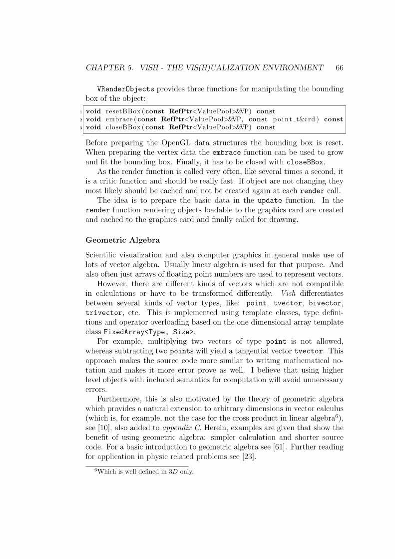
CHAPTER 5. VISH - THE VIS(H)UALIZATION ENVIRONMENT 66
VRenderObjects provides three functions for manipulating the boundingbox of the object:
1 void resetBBox ( const RefPtr<ValuePool>&VP) const2 void embrace ( const RefPtr<ValuePool>&VP, const p o i n t t&crd ) const3 void closeBBox ( const RefPtr<ValuePool>&VP) const
Before preparing the OpenGL data structures the bounding box is reset.When preparing the vertex data the embrace function can be used to growand fit the bounding box. Finally, it has to be closed with closeBBox.
As the render function is called very often, like several times a second, itis a critic function and should be really fast. If object are not changing theymost likely should be cached and not be created again at each render call.
The idea is to prepare the basic data in the update function. In therender function rendering objects loadable to the graphics card are createdand cached to the graphics card and finally called for drawing.
Geometric Algebra
Scientific visualization and also computer graphics in general make use oflots of vector algebra. Usually linear algebra is used for that purpose. Andalso often just arrays of floating point numbers are used to represent vectors.
However, there are different kinds of vectors which are not compatiblein calculations or have to be transformed differently. Vish differentiatesbetween several kinds of vector types, like: point, tvector, bivector,trivector, etc. This is implemented using template classes, type defini-tions and operator overloading based on the one dimensional array templateclass FixedArray<Type, Size>.
For example, multiplying two vectors of type point is not allowed,whereas subtracting two points will yield a tangential vector tvector. Thisapproach makes the source code more similar to writing mathematical no-tation and makes it more error prove as well. I believe that using higherlevel objects with included semantics for computation will avoid unnecessaryerrors.
Furthermore, this is also motivated by the theory of geometric algebrawhich provides a natural extension to arbitrary dimensions in vector calculus(which is, for example, not the case for the cross product in linear algebra6),see [10], also added to appendix C. Herein, examples are given that show thebenefit of using geometric algebra: simpler calculation and shorter sourcecode. For a basic introduction to geometric algebra see [61]. Further readingfor application in physic related problems see [23].
6Which is well defined in 3D only.
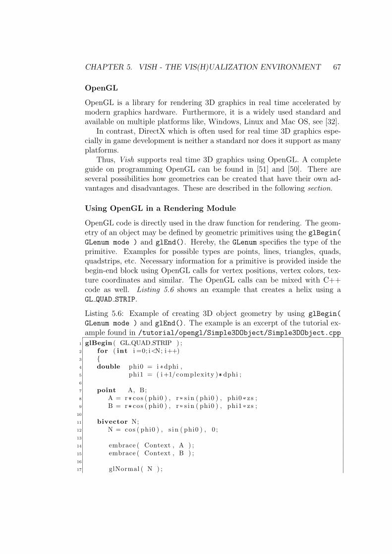
CHAPTER 5. VISH - THE VIS(H)UALIZATION ENVIRONMENT 67
OpenGL
OpenGL is a library for rendering 3D graphics in real time accelerated bymodern graphics hardware. Furthermore, it is a widely used standard andavailable on multiple platforms like, Windows, Linux and Mac OS, see [32].
In contrast, DirectX which is often used for real time 3D graphics espe-cially in game development is neither a standard nor does it support as manyplatforms.
Thus, Vish supports real time 3D graphics using OpenGL. A completeguide on programming OpenGL can be found in [51] and [50]. There areseveral possibilities how geometries can be created that have their own ad-vantages and disadvantages. These are described in the following section.
Using OpenGL in a Rendering Module
OpenGL code is directly used in the draw function for rendering. The geom-etry of an object may be defined by geometric primitives using the glBegin(
GLenum mode ) and glEnd(). Hereby, the GLenum specifies the type of theprimitive. Examples for possible types are points, lines, triangles, quads,quadstrips, etc. Necessary information for a primitive is provided inside thebegin-end block using OpenGL calls for vertex positions, vertex colors, tex-ture coordinates and similar. The OpenGL calls can be mixed with C++code as well. Listing 5.6 shows an example that creates a helix using aGL QUAD STRIP.
Listing 5.6: Example of creating 3D object geometry by using glBegin(
GLenum mode ) and glEnd(). The example is an excerpt of the tutorial ex-ample found in /tutorial/opengl/Simple3DObject/Simple3DObject.cpp
1 glBegin ( GL QUAD STRIP ) ;2 for ( int i =0; i<N; i++)3 4 double phi0 = i *dphi ,5 phi1 = ( i +1/complexity )* dphi ;6
7 point A, B;8 A = r * cos ( phi0 ) , r * s i n ( phi0 ) , phi0 * zs ;9 B = r * cos ( phi0 ) , r * s i n ( phi0 ) , phi1 * zs ;
10
11 bivector N;12 N = cos ( phi0 ) , s i n ( phi0 ) , 0 ;13
14 embrace ( Context , A ) ;15 embrace ( Context , B ) ;16
17 glNormal ( N ) ;

CHAPTER 5. VISH - THE VIS(H)UALIZATION ENVIRONMENT 68
Figure 5.4: Helix rendered by the OpenGL code shown in listing 5.6.
18 g lVertex ( A ) ;19 g lVertex ( B ) ;20 21 glEnd ( ) ;
Here, a strip of quad primitives is created by stepping forward in theloop and adding two vertices with the same surface normal. The glNormal
function encapsulates the OpenGL function glNormal3f for convenience andthe glVertex accordingly. Note, the usage of the VRenderModule memberfunction embrace to enlarge the objects bounding box on the fly, see listing5.6 line 14 and line 15.
This method can be very convenient for certain types of geometry butusually is very slow. While still using the same OpenGL calls this methodcan be accelerated drastically by compiling the calls into a so called displaylist. A pre compiled list of subsequent OpenGL commands will be executedmuch faster. To compile a display list in Vish use the macro glCompile( )
which basically encapsulates the OpenGL command glNewList(), as shownin listing 5.7.
Listing 5.7: Compiling a display list in Vish
1 RefPtr<Disp layLi s t > DL;2 glCompile ( *DL )3 4 glBegin ( /* . . . */ ) ;5 /* . . . */6 glEnd ( ) ;7
Of course, performance will only be gained when not recompiled withevery call of the VRenderObject’s code render function. Thus, the display
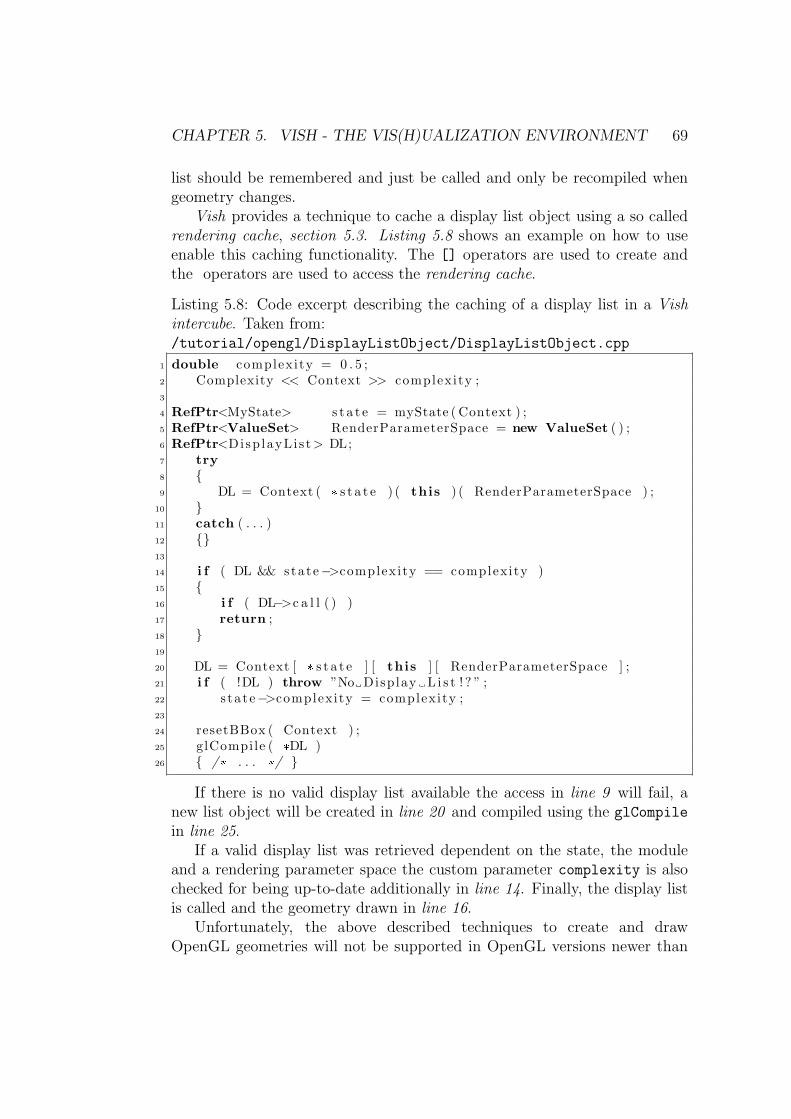
CHAPTER 5. VISH - THE VIS(H)UALIZATION ENVIRONMENT 69
list should be remembered and just be called and only be recompiled whengeometry changes.
Vish provides a technique to cache a display list object using a so calledrendering cache, section 5.3. Listing 5.8 shows an example on how to useenable this caching functionality. The [] operators are used to create andthe operators are used to access the rendering cache.
Listing 5.8: Code excerpt describing the caching of a display list in a Vishintercube. Taken from:/tutorial/opengl/DisplayListObject/DisplayListObject.cpp
1 double complexity = 0 . 5 ;2 Complexity << Context >> complexity ;3
4 RefPtr<MyState> s t a t e = myState ( Context ) ;5 RefPtr<ValueSet> RenderParameterSpace = new ValueSet ( ) ;6 RefPtr<Disp layLi s t > DL;7 try8 9 DL = Context ( * s t a t e ) ( this ) ( RenderParameterSpace ) ;
10 11 catch ( . . . )12 13
14 i f ( DL && state−>complexity == complexity )15 16 i f ( DL−>c a l l ( ) )17 return ;18 19
20 DL = Context [ * s t a t e ] [ this ] [ RenderParameterSpace ] ;21 i f ( !DL ) throw ”No Display L i s t ! ? ” ;22 s ta te−>complexity = complexity ;23
24 resetBBox ( Context ) ;25 glCompile ( *DL )26 /* . . . */
If there is no valid display list available the access in line 9 will fail, anew list object will be created in line 20 and compiled using the glCompile
in line 25.If a valid display list was retrieved dependent on the state, the module
and a rendering parameter space the custom parameter complexity is alsochecked for being up-to-date additionally in line 14. Finally, the display listis called and the geometry drawn in line 16.
Unfortunately, the above described techniques to create and drawOpenGL geometries will not be supported in OpenGL versions newer than
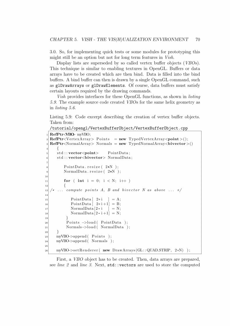
CHAPTER 5. VISH - THE VIS(H)UALIZATION ENVIRONMENT 70
3.0. So, for implementing quick tests or some modules for prototyping thismight still be an option but not for long term features in Vish.
Display lists are superseded by so called vertex buffer objects (VBOs).This technique is similar to enabling textures in OpenGL. Buffers or dataarrays have to be created which are then bind. Data is filled into the bindbuffers. A bind buffer can then is drawn by a single OpenGL command, suchas glDrawArrays or glDrawElements. Of course, data buffers must satisfycertain layouts required by the drawing commands.
Vish provides interfaces for these OpenGL functions, as shown in listing5.9. The example source code created VBOs for the same helix geometry asin listing 5.6.
Listing 5.9: Code excerpt describing the creation of vertex buffer objects.Taken from:/tutorial/opengl/VertexBufferObject/VertexBufferObject.cpp
1 RefPtr<VBO> myVBO;2 RefPtr<VertexArray> Points = new TypedVertexArray<point >() ;3 RefPtr<NormalArray> Normals = new TypedNormalArray<bivector >()4 5 std : : vector<point> PointData ;6 std : : vector<bivector> NormalData ;7
8 PointData . r e s i z e ( 2*N ) ;9 NormalData . r e s i z e ( 2*N ) ;
10
11 for ( int i = 0 ; i < N; i++ )12 13 /* . . . compute po in t s A, B and b i v e c t o r N as above . . . */14
15 PointData [ 2* i ] = A;16 PointData [ 2* i +1] = B;17 NormalData [2* i ] = N;18 NormalData [2* i +1] = N;19 20 Points −>load ( PointData ) ;21 Normals−>load ( NormalData ) ;22 23 myVBO−>append ( Points ) ;24 myVBO−>append ( Normals ) ;25
26 myVBO−>setRenderer ( new DrawArrays (GL : : QUAD STRIP, 2*N) ) ;
First, a VBO object has to be created. Then, data arrays are prepared,see line 2 and line 3. Next, std::vectors are used to store the computed

CHAPTER 5. VISH - THE VIS(H)UALIZATION ENVIRONMENT 71
geometry data in RAM7. When the data in RAM is complete it is loadedinto the data arrays and, thus, loaded in the memory of the graphics hard-ware, line 21 and line 22. The data arrays have to be appended to Vish’sVBO object and finally the renderer has to be configured with the correctinformation about the type and size of data, line 26.
Prepared VBO objects can be cached in the same way as a display list.Listing 5.10 shows the details.
Listing 5.10: Code excerpt describing the caching of vertex buffer objects.Taken from:/tutorial/opengl/VertexBufferObject/VertexBufferObject.cpp
1 RefPtr<MyState> s t a t e = myState ( Context ) ;2 RefPtr<ValueSet> RenderParamSpace = new ValueSet ( ) ;3 RefPtr<VBO> myVBO;4 try5 6 myVBO = Context (* s t a t e ) ( this )7 ( RenderParamSpace ) ( VERTEXBUFFER( ) ) ;8 9 catch ( . . . )
10 i f (myVBO && !myVBO−>empty ( ) && state−>complexity==complexity )11 12 i f (myVBO−>c a l l ( ) )13 return ;14 15
16 myVBO = Context [* s t a t e ] [ this ]17 [ RenderParamSpace ] ( VERTEXBUFFER( ) ) ;18
19 myVBO−>c l e a r ( ) ;20
21 s ta te−>complexity = complexity ;22
23 /* . . . f i l l VBO as de s c r i b ed above . . . */24
25 myVBO−>c a l l ( )
The only difference is the additional test if the VBO is empty in line 10.Otherwise it is totally equivalent to listing 5.8.
Shaders can also be used for rendering. Vish provides a class calledProgram for that purpose. The fragment, geometry or vertex shader code isthen stored in a static const char string.
Listing 5.11 shows how a shader program is created, line 4, how it isvalidated for correct syntax, line 7, and how it is activated for use, line 12.
7Random Access Memory

CHAPTER 5. VISH - THE VIS(H)UALIZATION ENVIRONMENT 72
Unexpected exceptions are caught in line 14. Uniform variables of the shadercode can be accessed using the setUniFormValue* member function of theProgram class.
Listing 5.11: Code excerpt describing how to use Program with a OpenGLshader.
1 RefPtr<Program>&MyProgram = FR. MyProgram ;2 try3 4 MyProgram = new Program( co lormap vertex shader ,5 co lormap fragment shader ) ;6
7 i f ( ! MyProgram−>i s V a l i d ( ) )8 9 puts ( ”MyRenderModule : i n v a l i d program ! ” ) ;
10 return ;11 12 MyProgram−>use ( ) ;13 14 catch ( const Program : : Error&E)15 16 E. p r in t ( ”Compiled program not usab le ” ) ;17 a s s e r t ( 0 ) ;18 19
20 MyProgram−>setUni formValue i ( ”volumedata” , 0 ) ;21 MyProgram−>setUni formValue i ( ” colormap” , 1 ) ;22
23 24 double va l = 1 . 0 ;25 Sharpness << Context >> va l ;26 MyProgram−>setUni formValuef ( ” Sharpness ” , s td : : exp (5* va l ) ) ;27 28 29 int N = 1 ;30 NumberOfPeaks << Context >> N;31 MyProgram−>setUni formValue i ( ”NumberOfPeaks” , N) ;32
For more information of shader programming in general, see [50] and formore examples in Vish see the tutorial section of Vish.
5.2.4 Vish Scripts
A simple script language is used to define networks in Vish. At the currentstate the script languages enables to create modules, to set parameter values,

CHAPTER 5. VISH - THE VIS(H)UALIZATION ENVIRONMENT 73
to connect parameters and to open *.f5 data files. It is a keyword freelanguage and supports UTF8.
A script file can be loaded by using the File->Open of the Vish GUIor by giving the script as the first parameter when starting Vish from thecommand shell, for example from the /data directory:
../bin/vish Analytic.vis
A new module can be created by using the name string of its VCreator.This string also is used to create the context menu for module creation inthe GUI, section 5.2. A module found in Utility/Point3D can be createdusing the same string followed by a name for the instance the module. Forexample:
Utility/Point3D myPoint
Parameter values can be set by using the name of the module instancefollowed by the name of the parameter to be set separated by a dot. Anequality followed by the value will set the parameter value. If the value is ofwrong type or if the value is out of range of the min and max properties ofthe parameter the script line will be ignored. For example:
myPoint.x=1.5
Setting a parameter can be done within the context of a certain view portwindow. A parameter can have different values in different view ports. Tospecify the view port use after the parameter name. For example:
myPoint.xViewer2=1.5A parameter can be connected to the an other parameter. Most fre-
quently it is connected to an output of another module. In that case it issufficient to specify the name of the module instance and the appropriateoutput parameter is found automatically. The => operator is used for pa-rameter connection. A connection can also be done to an explicit parameter.For example:
vertices.grid=>geodesics
To load an F5 file via script the @ symbol is used followed by the stringof the directory and filename enclosed by "". For example:
@"../data/mydata.f5"
The # symbol is used for comments. All characters after will be ignoreduntil the next newline.
Enclosing the name of a module instance by <> forces an update of themodule:

CHAPTER 5. VISH - THE VIS(H)UALIZATION ENVIRONMENT 74
<myPointViewer1>
Prefixing a ! in front of a name of a module instance will touch themodule and flags it for a required update:
!myPoint
The GUI frame showing the module can by minimized hiding all pa-rameter GUI controls. Then only the name of the module is shown in thenetwork, see left most figure of figure 5.3:
Network.iconify(myPoint)
Listing 5.12 shows a typical *.vis script using most of the script featuresdescribed above.
Listing 5.12: Typical vis script defining a Vish network. The example showsthe content of /fish/lakeview/cephalus/UnigridIsosurface.vis
1 CreateFiber / A n a l y t i c S c a l a r f i e l d A n a l y t i c S c a l a r F i e l d2 #A n a l y t i c S c a l a r F i e l d . spacet ime=>MyGrid . spacet ime3 #! A n a l y t i c S c a l a r F i e l d . a4 <A n a l y t i c S c a l a r F i e l d Viewer1>5
6 Colormaps/Colorramp Fie ldCo lo r s7 Display / OrthoS l i c e MyFie ldS l i ce8 MyFie ldS l i ce . colormap=>Fie ldCo lo r s9
10 MyFie ldS l i ce . s c a l a r f i e l d=>A n a l y t i c S c a l a r F i e l d11 MyGridBox . spacet ime=>A n a l y t i c S c a l a r F i e l d12
13 Network . i c o n i f y ( A n a l y t i c S c a l a r F i e l d )14 Network . i c o n i f y ( MyFie ldS l i ce )15 Network . i c o n i f y (MyGridBox)16
17 Display /BoundingVolume BVol18 BVol . source=>MyFie ldS l i ce19
20 Compute/ I s o S u r f a c e I s o S u r f a c e21 I s o S u r f a c e . s c a l a r f i e l d=>A n a l y t i c S c a l a r F i e l d22 I s o S u r f a c e . i s o l e v e l =0.523 #<I soSur face >24
25 Display / SurfaceView IsoView26 IsoView . g r id=>I s o S u r f a c e27 #<IsoViewViewer1>
CHAPTER 5. VISH - THE VIS(H)UALIZATION ENVIRONMENT 75
5.3 Caching
A good caching approach in the visualization network8 is identified as keyrequirement for interactive exploration of huge datasets. Caching avoidsunnecessary re-computations, speeds up computation and rendering, leadingto interactive frame rates that would not be possible otherwise.
Vish allows caching on three levels. Firstly, caching in a network mod-ule. Secondly, data can be cached at the any data sources, especially onFiber Bundle data sources and on data flow nodes itself. Finally, OpenGLdisplay lists and VBOs can be cached directly on the graphics hardware,section 5.2.3. All these caching techniques are used during the implementa-tion of the modules needed for visualizing geodesics.
Data can be cached or stored in the network module by using a State
object, section 5.2.1. This procedure is suitable for small sets of data, likeremembering a certain attribute value from a last call of update, to check ifit had been changed or similar. Data storage is kept outside the module.
The description below is following the content of [12], also included inappendix C.
Data can be cached in data sources. The data source itself has to be a socalled InterCube object, as described in [11]. A template class, the so calledOperatorCache is used to cache some computational results associated to theInterCube. Any class can inherit the InterCube properties be being derivedfrom the MemCore class InterCube. A data set like, for example, a vector ofdoubles can then be stored by initiating the template OperatorCache:
typedef OperatorCache<std::vector<double> > OC t;
”Now given an InterCube object provided to a computational routine,one may retrieve an OperatorCache object that may be stored there. If not,we would need to create one anyway:” [12]
1 void VizNode : : compute ( InterCube &MyData)2 3 OC t*OC = OC t : : r e t r i e v e ( MyData , this ) ;4 i f ( !OC ) OC = new OC t ( ) ;5
Data is retrieved from the InterCube dependent on the data type and thevisualization module. Data again is stored outside the local memory.
Needed re-computation, for example when certain parameters getchanged, can be decided by utilizing the unchanged() member function ofthe OperatorCache template. The function takes a ValueSet that is testedfor changes.
8or visualization cascade, in contrary to visualization pipeline
CHAPTER 5. VISH - THE VIS(H)UALIZATION ENVIRONMENT 76
Listing 5.13: Code fragment showing how to use a ValueSet of TypedSlotswith a OperatorCache.
1 RefPtr< ValueSet > Changeables = new ValueSet ( ) ;2
3 *Changeables <<= IsoValue ( Context ) ;4
5 i f ( OC−>unchanged ( Changeables ) )6 7 /* . . . do something wi th the data e x i s t i n g in OC . . . */8 return ;9
10 /* . . . compute new data and put them in to the OC . . . */
After a new ValueSet is created in line 1 the TypedSlot<double>
IsoValue is added to the set using the <<= operator in line 3. The Op-eratorCache is then queried with the ValueSet wheter something has to bedone or not.
Data can be cached in Fiber Bundle data sources inside a Fiber Bun-dle if it is stored as a Fiber Grid object, chapter 4. In that case the FiberGrid is identified by a double time and a string name for identification inthe Fiber Bundle. When additional values should influence the identificationthey just can be concatenated to the name string.
Listing 5.14: Example of caching a Fiber Grid in a Fiber Bundle. Based onthe example described in [12].
1 Grid VizNode : : compute (Bundle&B, double time ,2 string Gridname , string Fieldname ,3 double I s o l e v e l )4 5 string IsosurfaceName = Gridname + Fieldname + I s o l e v e l ;6
7 RefPtr<Grid> I s o S u r f a c e = B[ time ] [ IsosurfaceName ] ;8
9 i f ( ! I s o S u r f a c e )10 11 RefPtr<Grid> DataVolume = B[ time ] [ Gridname ] ;12 I s o S u r f a c e = Compute ( DataVolume , Fieldname , I s o l e v e l ) ;13
14 B[ time ] [ IsosurfaceName ] = I s o S u r f a c e ;15 16 return I s o S u r f a c e ;17
Listing 5.14 shows a source code example where a Fiber Grid object iscached in the Fiber Bundle. The caching is dependent on the actual time,the Fiber Grid and the Fiber Field names of the underlying data source
CHAPTER 5. VISH - THE VIS(H)UALIZATION ENVIRONMENT 77
and a parameter IsoLevel. The Fiber Grid object IsoSurface is computedand stored in the Fiber Bundle, line 11 to line 14. This is an expensiveoperation since the underlying data sets may have to be loaded from diskand the computation of the IsoSurface has to be done. In a second call ofthe VizNode::compute function this operations are skipped because it cansuccessfully retrieve the IsoSurface from the Fiber Bundle B in line 7.
5.4 Data Field Interpolation and Finding Lo-
cal Coordinates
While the Fiber Bundle library provides a clear and unified structure to storeall kinds of scientific data, working with the library itself still needs specialsome handling for different types, such as, checking for fragmented grids,checking for refinements levels and similar.
When developing visualization modules some of the required source codeis needed frequently in a similar fashion. There is still room for implement-ing convenience functions and classes that ease accessing Fiber Bundle datastructures.
In context of this work, for instance, the local index coordinates of a gridobject by a given world coordinate point had to be computed. The localindex coordinate is then used for data field interpolation. This is a commonapproach, see, for example, [18].
Figure 5.5 shows two 2 dimensional grids and a point described in localand in world coordinates. Computing local coordinates in an uniform regulargrid is straightforward by doing a linear interpolation of the local coordinatesof the cell that contains the point. But, when computing a local point in acurvilinear multi-block grid things become more difficult, especially whentrying algorithms must be fast.
The modules that needed local index computation should work with allpossible grid data structures. The calculation needs different handling de-pendent on the underlying data. Possible grids are uniform, multi-block,curvilinear or AMR grids.
I introduced a class called LocalPointFinder. It takes a Fiber Slice, aFiber Grid and the Fiber Field holding the coordinate values as parameterand provides a get function that returns a local coordinate and the fragmentID of the fragment that contains the point in case of multi-block data by agiven world coordinate value:
bool get( const point position, pair<point, string>&data );
Now, a developer of a module can conveniently get the local coordinates
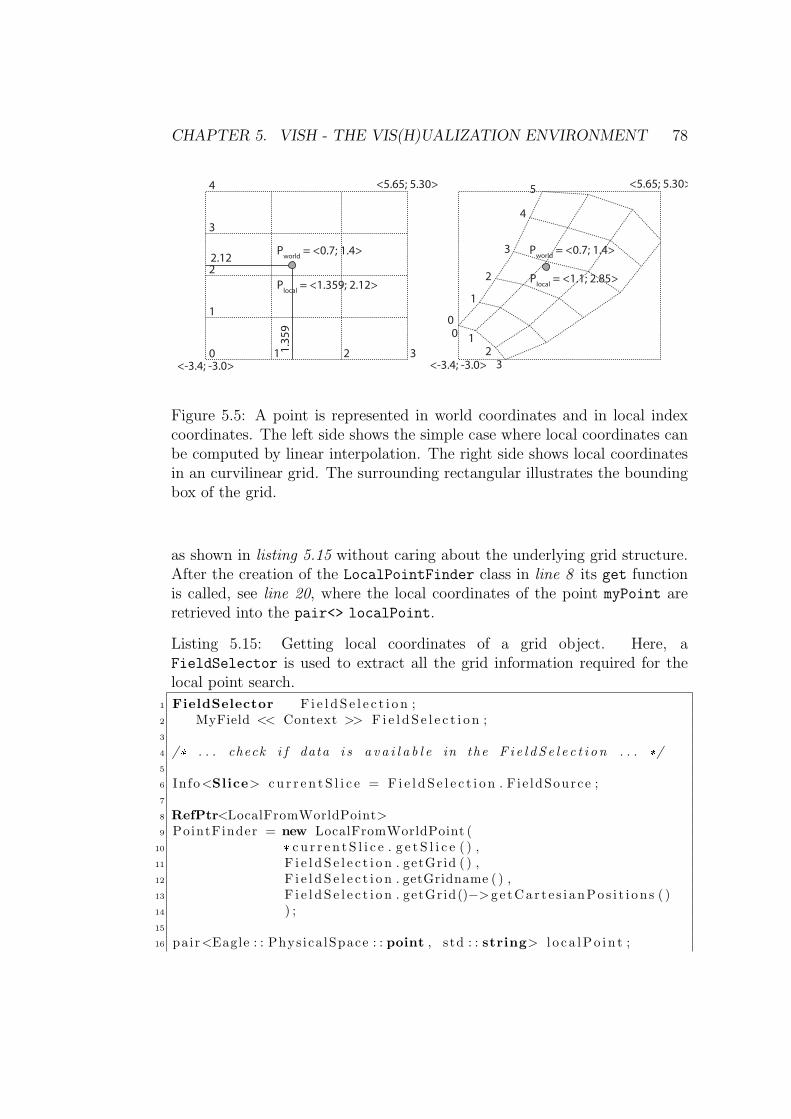
CHAPTER 5. VISH - THE VIS(H)UALIZATION ENVIRONMENT 78
21 30
1
2
3
4 <5.65; 5.30>
<-3.4; -3.0>
Pworld = <0.7; 1.4>
1.35
9
2.12
<-3.4; -3.0>
<5.65; 5.30>
0 12
3
0
1
2
3
4
5
Plocal = <1.359; 2.12>
Pworld = <0.7; 1.4>
Plocal = <1.1; 2.85>
Figure 5.5: A point is represented in world coordinates and in local indexcoordinates. The left side shows the simple case where local coordinates canbe computed by linear interpolation. The right side shows local coordinatesin an curvilinear grid. The surrounding rectangular illustrates the boundingbox of the grid.
as shown in listing 5.15 without caring about the underlying grid structure.After the creation of the LocalPointFinder class in line 8 its get functionis called, see line 20, where the local coordinates of the point myPoint areretrieved into the pair<> localPoint.
Listing 5.15: Getting local coordinates of a grid object. Here, aFieldSelector is used to extract all the grid information required for thelocal point search.
1 FieldSelector F i e l d S e l e c t i o n ;2 MyField << Context >> F i e l d S e l e c t i o n ;3
4 /* . . . check i f data i s a v a i l a b l e in the F i e l d S e l e c t i o n . . . */5
6 Info<Slice> c u r r e n t S l i c e = F i e l d S e l e c t i o n . F ie ldSource ;7
8 RefPtr<LocalFromWorldPoint>9 PointFinder = new LocalFromWorldPoint (
10 * c u r r e n t S l i c e . g e t S l i c e ( ) ,11 F i e l d S e l e c t i o n . getGrid ( ) ,12 F i e l d S e l e c t i o n . getGridname ( ) ,13 F i e l d S e l e c t i o n . getGrid()−> g e t C a r t e s i a n P o s i t i o n s ( )14 ) ;15
16 pair<Eagle : : Phys ica lSpace : : point , s td : : string> l o c a l P o i n t ;

CHAPTER 5. VISH - THE VIS(H)UALIZATION ENVIRONMENT 79
17
18 Eagle : : Phys ica lSpace : : point myPoint ( 0 . 2 , 0 . 1 , 4 . 4 ) ;19
20 bool t e s t = PointFinder . get ( myPoint , l o c a l P o i n t ) ;
The following sections describes more details of theLocalFromWorldPoint class in depth. The class itself was the resultof several rewritings and optimizations and finally became a part of the coreof the Fiber Bundle library, found in /fish/fiber/baseop.
5.4.1 UniGrid
The simplest case for computing a local coordinate applies to single-blockuniform regular grids. Utilizing a fragment iterator as described in chapter4 will automatically capture support for single and multi-block grids. Insidethe iterator it has to be checked if the vertex data is given procedurally.
To completely describe a uniform regular grid it is sufficient to know itsworld position bounds and the number of cells in each direction, chapter 4.
Getting this data is shown in listing 5.16. Line 8 checks if a proceduralProcArray t could be retrieved. If successful this describes a uniform regulargrid.
Listing 5.16: Example of checking for a simple uniform field and doing asimple linear interpolation to compute local index coordinates of a givenspace point.
1 RefPtr<Field> myField2 point p o s i t i o n ;3
4 /* . . . */5
6 RefPtr<ProcArray t> PCrd = coords−>getData ( ) ;7
8 i f ( PCrds )9
10 point DomainStart = PCrd−> f i r s t ( ) ;11 point DomainEnd = PCrd−>l a s t ( ) ;12 tvector DomainDiagonal = DomainEnd − DomainStart ;13
14 MultiIndex<3> FSize = PCrd−>S i z e ( ) ;15 point max f l oa t index ;16 max f l oa t index = FSize [0 ]−1 , FSize [1 ]−1 , FSize [2 ] −1 ;17
18 f l o a t i n d e x = point ( tvector ( component wise ( component wise (19 p o s i t i o n − DomainStart , DomainDiagonal ,20 Eagle : : Operator< ’ / ’ >() ) ,
CHAPTER 5. VISH - THE VIS(H)UALIZATION ENVIRONMENT 80
21 max f loat index , Eagle : : Operator< ’ * ’ >()) ) ) ;
The following code shows how to do the interpolation to compute lo-cal coordinates. The dimensions in all axis directions are stored in theDomainDiagonal. The maximal index length of the 3D data array is com-puted by (sizeX−1, sizeY −1, sizeZ−1), see line 18. Now, the interpolationis done by computing xlocal = xpos−xstart
xinterval(maxindexx) in all dimensions simul-
taneously using the component wise template. This allows to do mathemat-ical operations component wise on a FixedArray<> and furthermore enablesthe use of SIMD instructions on the processor, if possible.
5.4.2 Multiblock
When dealing with a multi-block dataset at first the block that containsthe world point has to be found. The fragments itself may be uniform orcurvilinear.
A simple and quick to implement solution would be to do an iterationover all fragments and test if a fragment’s bounding box contains the worldpoint. However, when having thousands of block more sophisticated methodscan speed up the search drastically.
In case of fragmented uniform data just one fragment would be found asa result of a testing bounding boxes. When dealing with curvilinear gridsmore than one fragment can be found that contains the world point, becauseboundinx boxes overlap, see figure 5.7.
I chose a binary tree search for finding candidate multi-block. A KDTreeis utilizzed. Distances to the center of candidate fragments are computedand returned into a STL container.
I implemented an N dimensional KDTree based on John TsiombikasC implementation (http://code.google.com/p/kdtree/). It was almostcompletely rewritten using C++ template programming.
The tree stores any data elements at a N dimensional position. When alldata was inserted into the tree a range query can be done by specifying a Ndimensional position and a distance. All data elements inside this distanceare then returned.
Figure 5.6 shows the geometrical structure of a KDTree. Data positionsare inserted into the tree. A new data position is stored left of right of theparent position. Thus, the inserted data position splits the space in two“child” regions. On each level of the tree nodes the direction of the splittingis switched. In 2D the space is split by alternating lines in x and y direction.In 3D space is split by alternating planes or bivectors with normals in x, yand z direction.

CHAPTER 5. VISH - THE VIS(H)UALIZATION ENVIRONMENT 81
1
2
3
4
5
6
78
1
4
5
2
3
6
78
1
6 2
58
7 4
3
Figure 5.6: Left: Geometrical illustration of a KDTree. Points are added intothe tree in order of their numeration. Each insertion splits the space in tworegions: left and right or bottom and top. If a point is added it is insertedas left or right child node dependent on the position of the parent. On eachtree level the direction of the splitting axis is alternated and the remainingsubspace is split. Right: Tree structure of objects. Each node can have a leftand a right child. The tree corresponds to the positions on the left. Bottomnodes are inserted left and top nodes right.

CHAPTER 5. VISH - THE VIS(H)UALIZATION ENVIRONMENT 82
Listing 5.17 shows the structure of the KDTree class. The template pa-rameters are int N for the dimension of the used space or the dimension ofthe locations where data is stored and class T for an arbitrary data type.It is derived from MemCore::ReferenceBase to enable reference counting forKDTree pointers.
The tree itself is build from tree nodes. Every node has a left and aright child and stores the data T data at the N dimensional position pos.Additionally the direction of the splitting has to be remembered for eachnode. The tree node is implemented as an inner struct Node of KDTree, seeline 4.
When new data is inserted into the tree, only one coordinate of the N -dimensional position is checked whether it is located left or right of thecurrent node. The current splitting coordinate is stored in the dir memberof the node. If a leaf node is reached the position and its associated data isadded as a left or right child.
The Node’s insert function is defined recursively, line 22. The KDTree’sinsert function just handles the right start case and starting insertion at itsroot Node, line 39.
Listing 5.17: Class header of the KDTree class.
1 template<int N, class T>2 class KDTree : public MemCore : : ReferenceBase<KDTree<N,T> >3 4 struct Node5 6 FixedArray<double , N> pos ;7 int d i r ;8 T data ;9 Node* l e f t ;
10 Node* r i g h t ;11
12 Node ( const FixedArray<double , N>&posP ,13 const int dirP , const T dataP )14 : pos ( posP ) , d i r ( dirP ) , data ( dataP ) , l e f t ( 0 ) , r i g h t (0 ) 15
16 ˜Node ( ) ;17
18 template<class Functor>19 void cal lFromFar ( const FixedArray<double , N>&queryPos ,20 Functor&func ) ;21
22 void i n s e r t r e c ( const FixedArray<double , N>&posP ,23 const T&data ) ;24
25 template <class Container>

CHAPTER 5. VISH - THE VIS(H)UALIZATION ENVIRONMENT 83
26 void f i n d n e a r e s t ( const FixedArray<double ,N>&posP ,27 double range , Container&l i s t ) ;28
29 ;30 Node* root ;31
32 public :33 KDTree ( )34 : MemCore : : ReferenceBase<KDTree<N,T> >(this )35 , root (0 ) , min range ( 0 . 0 ) 36
37 ˜KDTree ( ) ;38
39 void i n s e r t ( const FixedArray<double , N>&pos ,40 const T&data ) ;41
42 template<class Container>43 bool nea r e s t r ange ( const FixedArray<double , N>&pos ,44 const double range ,45 Container&r e s ) ;46
47 template<class Functor>48 void cal lFromFar ( const FixedArray<double , N>&queryPos ,49 Functor&func ) ;
The nearest range function utilizes the split space information to speedup the recursive range check. Many unlikely candidates can be excluded fromthe range test. A N -dimension position, a range value and a container haveto be specified as parameters.
The function uses a template call-back to fill an container defined as atype trait, section 3.1. Support for any container can be added by templatespecialization of KDTreeResult as shown in listing 5.18. Data insertion isencapsulated by the insert function of the type trait, see line 13.
The container itself is passed as a reference to the nearest range func-tion. This example shows how a STL multimap can now be used to returnresults of a tree query. The data elements of the tree and the squared dis-tance are returned as a multimap. Data insertion automatically sorts theelements by its distances.
Any other data container can be utilized by adding the according trait.The KDTree is thus independent of the container type and highly reusable,as suggested in [31].
Listing 5.18: Adding a container type that can be filled with results from aKDTreff range query.
1 template<class Container>2 struct KDTreeResult ;
CHAPTER 5. VISH - THE VIS(H)UALIZATION ENVIRONMENT 84
3
4 template<class T>5 struct KDTreeResult<std : : multimap<double ,T> >6 7 std : : multimap<double ,T> & r e s u l t ;8
9 KDTreeResult ( std : : multimap<double ,T>&r )10 : r e s u l t ( r )11 12
13 void i n s e r t ( const double d i s t s q , const T&data )14 15 r e s u l t . i n s e r t ( std : : pa ir<double ,T>( d i s t s q , data ) ) ;16 17 ;
Listing 5.19 shows the usage of the KDtree. A four dimensional tree iscreated. Data is filled into the tree. Then a multi-map container is preparedin line 12 and used for the range query at querypos with range 0.5 in line16.
Listing 5.19: Using the KDTree.
1 RefPtr<KDTree<4, int> >t r e e = new KDTree<4, int >() ;2
3 FixedArray<double , 4> querypos , pos1 , pos2 ;4 pos1 = 0 . 0 , 0 . 0 , 0 . 0 , 0 . 0 ;5 pos2 = 0 . 5 , 0 . 0 , 0 . 0 , 0 . 1 ;6
7 t ree−>i n s e r t ( pos1 , 1 ) ;8 t ree−>i n s e r t ( pos2 , 2 ) ;9
10 /* . . . i n s e r t much more i n t data . . . */11
12 s t l : : multimap<double , int>res map ;13
14 querypos = 0 . 1 , 0 . 1 , 0 . 1 , 0 . 1 ;15
16 t ree−>nea r e s t r ange ( querypos , 0 . 5 , res map )
Such a KDTree is used in the LocalFromWorldPoint class to chose can-didate fragments. In case of a fragmented vertex field a KDTree is createdin the constructor of LocalFromWorldPoint by iterating over all fragments,computing the center of each fragment and storing the fragment index at itscenter positions into a 3D KDTree.
Since the KDTree only has to be computed once for a fragmented gridobject it is cached using an InterCube object to the coordinate field. Toenable this feature an additional wrapper template class has to be provided
CHAPTER 5. VISH - THE VIS(H)UALIZATION ENVIRONMENT 85
that extends the KDTree by an additional interface, see listing 5.20.
Listing 5.20: Allow a KDTree to be stored in an Vish InterCube by derivingfrom Memcore::Interface<>
1 template<int N, class T>2 struct KDInterface : public MemCore : : I n t e r f a c e <KDTree<N, T> >3 4 MemCore : : RefPtr<KDTree<N, T> > Tree ;5
6 KDInterface ( const MemCore : : RefPtr<KDTree<N, T> > TreeP )7 : Tree ( TreeP )8 9 ;
In the constructor of LocalFromWorldPoint the KDTree is cached to thevertex field RefPtr<Field> coords:
1 RefPtr<KDTree<3, int> > MyTree ;2
3 RefPtr<KDInterface <3, int> >4 TreeInt = coords−>f i n d I n t e r f a c e ( typeid (KDTree<3, int>) ) ;5
6 i f ( ! TreeInt )7 8 MyTree = new KDTree<3, int >() ;9 TreeInt = new KDInterface <3, int >( MyTree ) ;
10 coords−>addIn t e r f a c e ( TreeInt ) ;11 12 else13 14 MyTree = TreeInt−>Tree ;15
Besides storing the centers and the fragment numbers, also the size orbounding radius of the largest fragment is stored. This maximal boundingradius is used for the tree range queries. This ensures that no fragmentcandidates are missed. Figure 5.7 illustrates an example in 2D showingfragments, midpoints, the query point and the query range.
Having found these candidates a more accurate test has to be done tofind the correct fragment and fragment cell, that contains the world point.
5.4.3 Curvilinear
Finding a the containing cell in a arbitrary curvilinear hexahedral cell in acurvilinear grid turned out to be a non trivial problem.

CHAPTER 5. VISH - THE VIS(H)UALIZATION ENVIRONMENT 86
BoundingBox Curvilinear Grid
Mid Point
max
Range Query
Figure 5.7: KDtree used for a range query on mid points of bounding boxes ofcurvilinear multi-blocks. Left: Bounding boxes of curvilinear blocks. Right:Mid points of bounding boxes. The maximum diagonal of all bounding boxesis used as the diameter of the range check at an arbitrary position (black dot).
Local Coordinates in one Hexahedral Cell
First I tried to find a map to transform a point from world coordinates tolocal coordinates when it is already known that the point is located insidea cell. I reduced to a two dimensional case for investigation. In that case ageneral four sided polygon have to be mapped to a normalized square of size1.0, see figure 5.9.
Though, on the first glance, it looked similar to barycentric coordinatesin a triangle, the additional geometry constrains turned out to lead to a nonconform mapping, in contrast to the linear mapping in case of a triangle.Besides just mapping the corner points also all four boundary lines must becontinuously constrained to the borders.
I finally found a suitable transformation method applicable to general 3Dhexahedral cells in [54]:
A world point p(u, v, w), with u, v and w being local coordinates in thecurvilinear cell can be computed using the following trilinear interpolationof the world coordinates of the eight corner points p0, p1 ... p7:
p(u, v, w) = (1− u)(1− v)(1− w) · p0 + u(1− v)(1− w) · p1+(1− u)v(1− w) · p2 + (1− u)(1− v)w · p3+
uv(1− w) · p4 + u(1− v)w · p5+(1− u)vw · p6 + uvw · p7
(5.1)
Given a point p∗(x, y, z) in world coordinates the local coordinates u, v, ware found by using an iteration method. First, a point p(u, v, w) is guessed
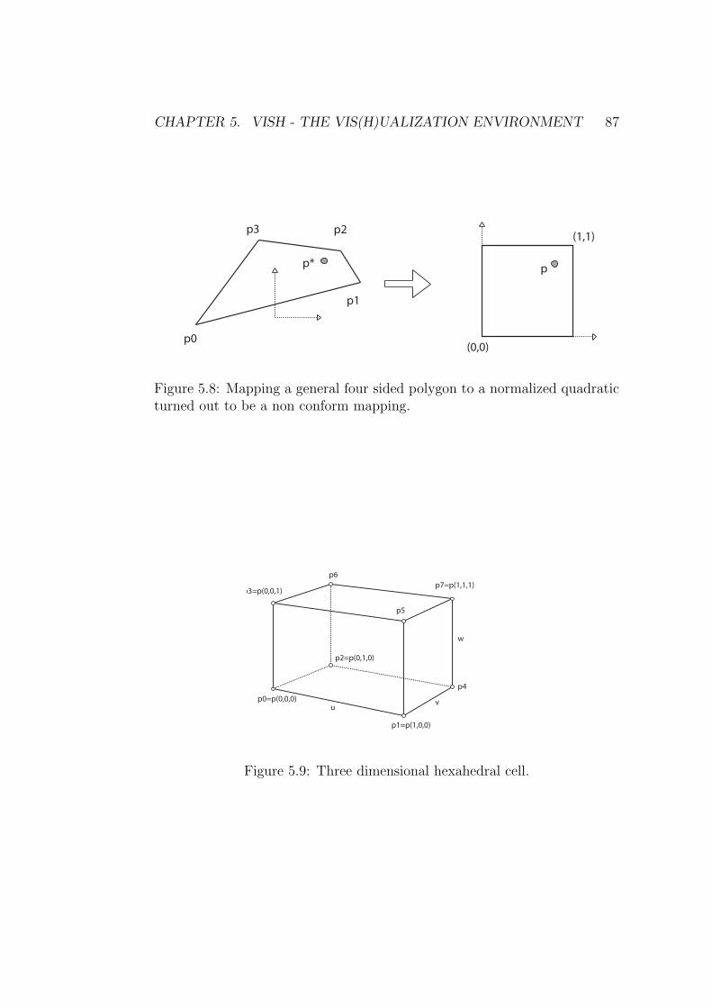
CHAPTER 5. VISH - THE VIS(H)UALIZATION ENVIRONMENT 87
p0
p1
p2p3
(0,0)
(1,1)
p* p
Figure 5.8: Mapping a general four sided polygon to a normalized quadraticturned out to be a non conform mapping.
uv
w
p0=p(0,0,0)
p7=p(1,1,1)
p1=p(1,0,0)
p2=p(0,1,0)
p3=p(0,0,1)
p4
p5
p6
Figure 5.9: Three dimensional hexahedral cell.

CHAPTER 5. VISH - THE VIS(H)UALIZATION ENVIRONMENT 88
inside the cell assuming certain local coordinates. I choose u = v = w = 0.5the point in the center of the cell. The Taylor series expansion of equation(5.1) yields:
p(u+ δu, v + δv, w + δw) = (5.2)
= p(u, v, w) +∂p
∂uδu+
∂p
∂vδv +
∂p
∂wδw +
+ O(δu2) +O(δv2) +O(δw2)
with:
∂p
∂u= (1− v)(1− w)(p1 − p0) + v(1− w)(p4 − p2)+ (5.3)
+ (1− v)w(p5 − p3) + vw(p7 − p6)
∂p
∂v= (1− u)(1− w)(p2 − p0) + u(1− w)(p4 − p1)+ (5.4)
+ (1− u)w(p6 − p3) + uw(p7 − p5)
∂p
∂w= (1− u)(1− v)(p3 − p0) + u(1− v)(p5 − p1)+ (5.5)
+ (1− u)v(p6 − p2) + uv(p7 − p4)
(5.6)
The desired increments δu, δv and δw can be computed by solving thefollowing linear 3× 3 equation system:
∂p
∂uδu+
∂p
∂vδv +
∂p
∂wδw = p∗ − p (5.7)
Using the computed increments of the equation system a new point pis computed using equation (5.1). Using the new point new derivatives arecomputed and the linear system is solved, again. This is repeated until||p∗ − p|| falls under a certain threshold.
In the implemented algorithm a threshold of approximately 1/100th
of the cells size is used which is computed once in the constructor ofUniGridMapper, see below.
Typically finding the local point requires one to two iteration steps to dropunder the threshold. If the cell is distorted heavily the number of iterationsincreases.
This algorithm is also used to test if a point is contained in a certain cell.In that case the result must be inside (0, 0, 0) and (1, 1, 1).
The algorithm is used for two purposes. Firstly, to check if a point islocated inside a cell, and secondly for the computation of the local hexahedralgrid coordinates, which is already computed during the first test.

CHAPTER 5. VISH - THE VIS(H)UALIZATION ENVIRONMENT 89
P
UniGridMapper
Curvilinear GridCurvilinear Cell Candidates
Figure 5.10: A curvilinear grid assigned to an uniform grid. The Uni-GridMapper provides a mapping from one uniform grid cell to curvilinearcells that touch it.
Finding Candidates in the Grid
When applying the test to a grid of curvilinear cells this would have to bedone for all cells until the containing cells is found.
To speed up the search within a curvilinear grid I introduced a new datastructure that reduces the number of cells to a few candidate cells for thetesting, analogously to the KDTree for multi-blocks.
The idea was to create a uniform grid that matches the size of the bound-ing box of the curvilinear grid and then provide a map from uniform cells tocurvilinear cells. Curvilinear cells touching a uniform grid cell are assigned tothe uniform cell. Figure 5.10 illustrates the method. The example illustratesthe mapping of one uniform grid cell (fat dashed line) to four curvilinear cells(fat line). All other uniform grid cells provide a similar mapping.
I called the introduced class UniGridMapper. It provides the mappingsfor one curvilinear block. The UniGridMapper stores a list of indices ofcurvilinear cells that is accessed by the index of the uniform grid cell.
These lists are generated in the constructor of the class, providing thefull mapping afterwards. While doing the iteration over all curvilinear cellsalso the bounding box of the UniGridMapper is computed and the averageedge length of all curvilinear cells. The average edge length, or better, its1/100th, is used for stopping the newton iteration as described earlier. Thesignature of the constructor is showed in listing 5.21.
Listing 5.21: Some interface details of class UniGridMapper

CHAPTER 5. VISH - THE VIS(H)UALIZATION ENVIRONMENT 90
1 typedef MemArray<3, point> CoordsArray t ;2
3 UniGridMapper ( const RefPtr<CoordsArray t>& CurviCoords ,4 const double r e s s c a l e = 1 . 0 ,5 const double p r e c s c a l e = 1 .0 ) ;6
7 /* . . . */8
9 unsigned10 l oca lCe l lCoordinatesFromCurviGr id ( const point & p , point & uvw ,11 double g r i d e p s i l o n = 0 . 0 ) ;12 /* . . . */
A MemArray holding the coordinates of the curvilinear block must beprovided. Optional parameters control the resolution of the uniform grid,line 4, and the precision of the reached newton iteration, line 5. Figure 5.11shows different resolutions of the uniform grid.
The UnigridMapper class also implements the iteration methodfor the local coordinate computation, by providing the functionlocalCellCoordinatesFromCurviGrid, see line 10.
When calling the function the list of curvilinear cells mapped to theaccording uniform grid cell are tested with the iteration method. Here, aproblem arose at the borders of the curvilinear cells. Due to numerical in-accuracies it could happen, that a point was located slightly outside of, forexample, four neighbored curvilinear cells.
To avoid to introduce epsilon tests I introduced a distance measure fromthe computed point to the closest borders of the cell. If none of the candidatecell contains a local point directly the “best” point, closest to a cell boundaryis returned.
Listing 5.22 shows the neighbor test in line 17. The DistPoint t struct
is used to store possible points with distance and curvilinear cell index ina container, line 11 and line 32. The city block (Manhattan) distance iscomputed in the for loop in line 22.
Listing 5.22: Handling local coordinates that are not found correctly at theborders of curvilinear cells
1 struct Dis tPo in t t2 3 double d i s t ;4 point uvw ;5 MultiIndex<3> s e l f ;6 ;7
8 /* . . . */9
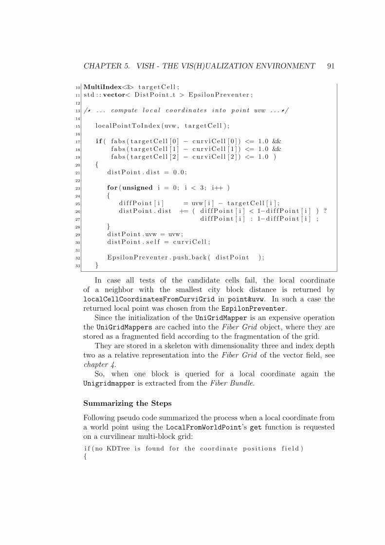
CHAPTER 5. VISH - THE VIS(H)UALIZATION ENVIRONMENT 91
10 MultiIndex<3> t a r g e t C e l l ;11 std : : vector< Dis tPo in t t > Eps i lonPreventer ;12
13 /* . . . compute l o c a l coord ina t e s in t o po in t uvw . . . */14
15 l oca lPo intToIndex (uvw , t a r g e t C e l l ) ;16
17 i f ( f abs ( t a r g e t C e l l [ 0 ] − c u r v i C e l l [ 0 ] ) <= 1.0 &&18 f abs ( t a r g e t C e l l [ 1 ] − c u r v i C e l l [ 1 ] ) <= 1.0 &&19 f abs ( t a r g e t C e l l [ 2 ] − c u r v i C e l l [ 2 ] ) <= 1.0 )20 21 d i s tPo in t . d i s t = 0 . 0 ;22
23 for (unsigned i = 0 ; i < 3 ; i++ )24 25 d i f f P o i n t [ i ] = uvw [ i ] − t a r g e t C e l l [ i ] ;26 d i s tPo in t . d i s t += ( d i f f P o i n t [ i ] < 1−d i f f P o i n t [ i ] ) ?27 d i f f P o i n t [ i ] : 1−d i f f P o i n t [ i ] ;28 29 d i s tPo in t . uvw = uvw ;30 d i s tPo in t . s e l f = c u r v i C e l l ;31
32 Eps i lonPreventer . push back ( d i s tPo in t ) ;33
In case all tests of the candidate cells fail, the local coordinateof a neighbor with the smallest city block distance is returned bylocalCellCoordinatesFromCurviGrid in point&uvw. In such a case thereturned local point was chosen from the EspilonPreventer.
Since the initialization of the UniGridMapper is an expensive operationthe UniGridMappers are cached into the Fiber Grid object, where they arestored as a fragmented field according to the fragmentation of the grid.
They are stored in a skeleton with dimensionality three and index depthtwo as a relative representation into the Fiber Grid of the vector field, seechapter 4.
So, when one block is queried for a local coordinate again theUnigridmapper is extracted from the Fiber Bundle.
Summarizing the Steps
Following pseudo code summarized the process when a local coordinate froma world point using the LocalFromWorldPoint’s get function is requestedon a curvilinear multi-block grid:
i f ( no KDTree i s found f o r the coord inate p o s i t i o n s f i e l d )

CHAPTER 5. VISH - THE VIS(H)UALIZATION ENVIRONMENT 92
Figure 5.11: Graphical output of a rendering module for visually debuggingthe method used to find a local coordinate. A curvilinear grid (dark grey) issurrounded by a UniGridMapper (light grey). The world point used for thesearch is shown colored red. If a local point is found, within the threshold, it isrecomputed to world coordinates by linear interpolation and drawn in green.The containing uniform cell is marked in red and the curvilinear cell is markedin yellow. The pictures show different resolutions chosen in the uniform grid:very low resolution on the left and higher resolution on the right. The modulecan be found in /fish/lakeview/eye/retina/FindLocalCoordinates.cpp
and the illustrated scene can be started with the according .vis script locatedin the same directory

CHAPTER 5. VISH - THE VIS(H)UALIZATION ENVIRONMENT 93
*Compute KDTree by i n s e r t i n g fragment IDs at cente r p o s i t i o n so f multi−b locks .
* cache KDTree as Inte rcube to the coord inate p o s i t i o n s .e l s e
*Get KDTree from cache .
*Do a range t r e e query at the world p o s i t i o n and r e t r i e v ecandidate fragments .
f o r ( each fragment candidate )
i f ( no UniGrimapper i s found in the bundle f o r the fragment )*Create UniGridmapper and s t o r e i t in the bundle .
e l s e*Get Unigridmapper from bundle .
*Get candidate c u r v i l i n e a r c e l l s from the UniGridmapper .
f o r ( each candidate c e l l )
*Use i t e r a t i o n to f i n d l o c a l coo rd inate .*Return a v a l i d l o c a l coo rd inate .
5.5 Basic Visualization Modules
During the development of the visualization modules and infrastructureneeded for geodesics I implemented some useful basic features along the way.Here, five tools are presented that enhance any data visualization in Vish.Two tools display coordinates, one shows the resolution of a uniform grid,one labels colors of a color map with data values and one draws outlines ofa multi-block grid.
5.5.1 Coordinate Grid
Displaying a coordinate plane is a very basic and helpful tool when analyzing3D data. The implemented module is a simple rendering module with norequired input connections. Coordinates are displayed as lines on a plane.A line is drawn at every multiple of 10 and every 10th line is labeled by itscoordinate value. The main parameters of the module control the alignment,the size, the refinement, the offset, the font size and font position.

CHAPTER 5. VISH - THE VIS(H)UALIZATION ENVIRONMENT 94
Figure 5.12: Coordinate Grid. A simple rendering module displaying basiscoordinate planes and coordinate values.
The coordinate plane can be aligned in the xy, xz, and yz plane. The sizecan be fixed or be adjusted dynamically dependent on the camera distance.If the size is controlled dynamically the size on screen will be constant whenzooming the camera. The refinement of the coordinate plane is always ad-justed dynamically. But, one can choose between three levels of refinement:normal, coarse and fine (finercoarser).
The coordinate plane can be shifted in direction of its normal by a theoffset parameter. Finally, the font size and the position can be controlled.The distance between the border of the grid object and the font can beset and a roll parameter defines the rotation around the coordinate planenormal. The coordinate values are displayed in engineering convention usingthe exponential notation.
5.5.2 Coordinate Grid Box
Another tool for analyzing 3D data and viewing its dimensions is the coordi-nate grid box. It is a rendering module that visualizes a connected boundingbox. It also draws “rulers” on three main axis at multiples of 10 of thecoordinates and labels the rulers with coordinate values.
The important attributes are used to control the ruler refinement, rulersize and the size, position and rotation of the coordinate labels.

CHAPTER 5. VISH - THE VIS(H)UALIZATION ENVIRONMENT 95
Figure 5.13: Coordinate Grid Box. A rendering module that displays thebounds of a bounding box and labels coordinate axes with numbers.
5.5.3 Uniform Grid Lines
The GridLines visualizes the grid resolution of a 3D uniform grid. Eitherthe xy, xz or yz plane is shown. Therefore, a Fiber Grid must be connectedto the module. Some basic parameters such as color, colorscale and an offsetvalue are provided. The offset changes the position of the coordinate planealong its normal direction.
Figure 5.14 illustrates the resolution of a uniform grid by showing abounding box and three coordinate planes drawn by three GridLine ren-dering modules. Here, the xy plane has no offset, whereas the two otherplanes have an offset of 0.5 moving the planes to the center of the grid.
5.5.4 Color Map Legend
When color maps are used to display some scalar fields then it is importantto know and see the mapping between colors and scalar values. Vish had nosuch tool. It is common practice to show a color map using a colored bar andlabeling numbers in the screen space9, for example at the lower right cornerof the 3D view.
First, I planned to create one single module to display color bar andnumber values. But then I recognized that it would be much more flexiblewhen separating into two distinct modules, one for the bar and one for thelabels. The labeling module would then be ’docked’ to the color bar module.
9camera image plane

CHAPTER 5. VISH - THE VIS(H)UALIZATION ENVIRONMENT 96
Figure 5.14: Uniform Grid Lines. A rendering module that displays the gridresolution of a uniform grid. Here, three modules are used for drawing threeaxis oriented planes illustrating the resolution.
Figure 5.15: Color Legend rendered by two distinct modules. One for thecolor bar and one for the labels.

CHAPTER 5. VISH - THE VIS(H)UALIZATION ENVIRONMENT 97
That way the labeling module would be easily replaceable be other modules,like a module that could display a histogram.
The basic idea was to build atomic components for HUD10 nodes thatcan be connected and combined in different ways.
To specify a position in screen space a new attribute type was introduced:Point2D. Coordinates in screen space are normalized and run from 0.0 to 1.0in x and y direction. A HUD component takes a 2D position as input andoutputs a 2D position as output, that another docking components then cantake as an input.
The attributes to control the color bar module ColorLegend are the po-sition, the height, the width and some attributes that control its appearance.The most important input attribute is the TypedSlot<VColormap> wherethe color map to be visualized is connected.
The module for number labeling is called RangeHUD. It has an input at-tribute for position and some attributes for configuration, like subdivision,which controls the number of displayed values and an attribute for font size.The main input attribute is a TypedSlot<Range> that defines the numberinterval. To synchronize the height of the labeling ruler with the height ofthe ColorLegend an additional input slot height is connected.
Figure 5.15 shows the graphical result of a ColorLegend connected byposition and height to a RangeHUD. Figure 5.16 shows the necessary Vishnetwork. Here, the connections described above are illustrated. A color mapmodule is connected to the ColorLegend and a range module is connectedto the RangeHUD. A Point2D module is connected to the ColorLegend mod-ule controling the overall position of the two HUD modules. RangeHUD isconnected to ColorLegend by position and height, as stated above.
5.5.5 Multiblock Outlines
During development of algorithms dealing with curvilinear multi-blockdatasets it became necessary, especially for visual debugging, to display theboundaries of all or some selected multi-blocks.
Thus, I added a rendering module that iterates over the Fiber Grid frag-ments of a dataset and extracts and renders the outlines of a multi-blockdataset. Attributes are provided to control the transparency and color ofthe outlines. Later, a filter was added, such that only those multi-blocks aredrawn that had a UniGridMapper object associated, section 5.4. Figure 5.17shows an example of 2088 curvilinear multi-blocks.
10head up display
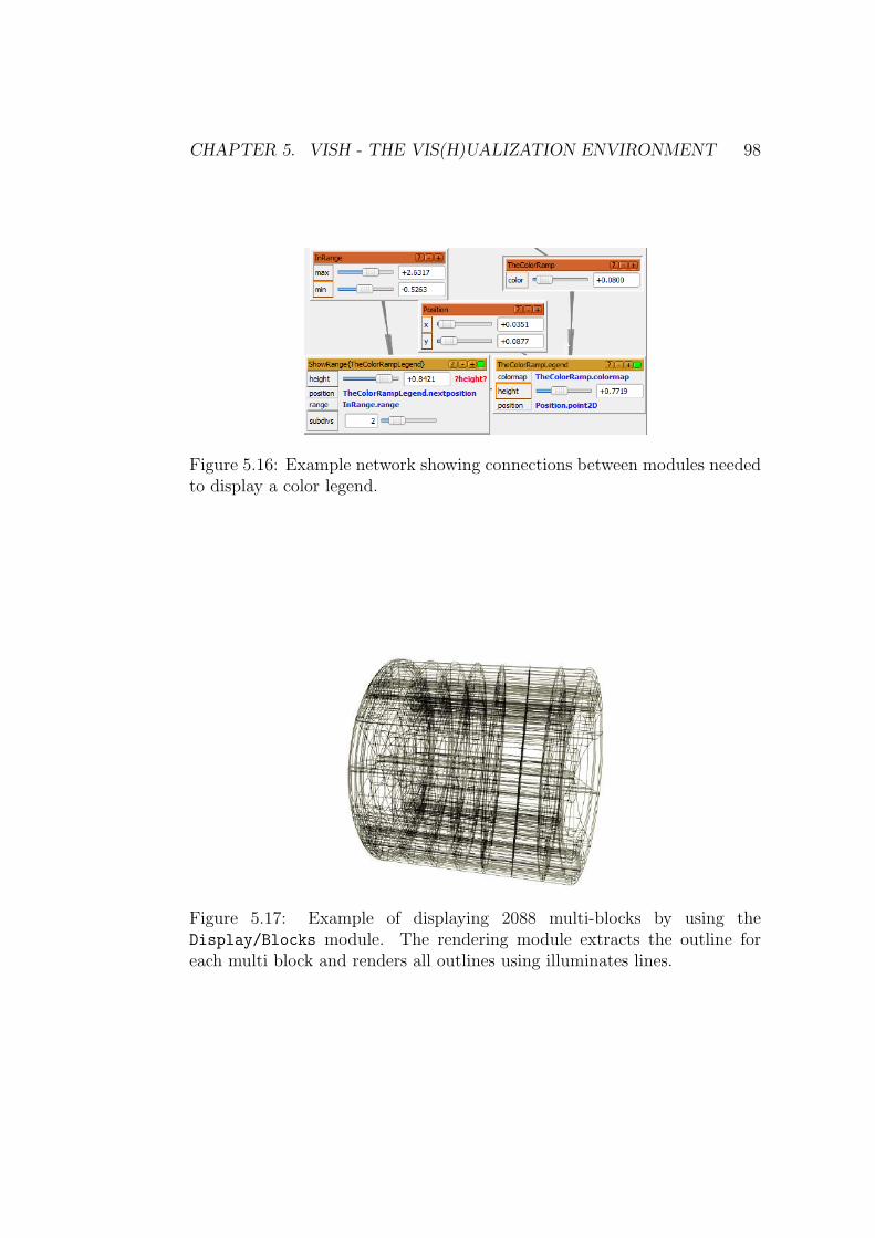
CHAPTER 5. VISH - THE VIS(H)UALIZATION ENVIRONMENT 98
Figure 5.16: Example network showing connections between modules neededto display a color legend.
Figure 5.17: Example of displaying 2088 multi-blocks by using theDisplay/Blocks module. The rendering module extracts the outline foreach multi block and renders all outlines using illuminates lines.

Chapter 6
Computation and Visualization
The first approach for computing and visualizing integral lines that was im-plemented was a short all-in-one Vish module. It received a procedural vectorfield as input. Streamlines were computed using a simple Euler integration,as described in section 6.2. Initial seed points were located on a fax in thexy-plane and could be moved around. Also the line rendering was done inthe same module.
It took me just four days to implement this 400 lines of code Vish moduleand I learned a lot about the software environments and the requirementsfor integral line visualization. Now it can be found in the tutorial section ofVish: SimpleStreamline.cpp.
I recognized that the flexibility of the basic approach can be increasedby separating the whole process into small tasks. The visualization processshould be split into three basic modules:
Define seeding geometry, or initial conditions.
Do the integration.
Render integration lines.
Thus, for all of these module types different modules could be implementedand assembled like building blocks according to the requirements of the vi-sualization.
This chapter first describes modules that were developed for defining theseeding geometry, then introduces the implemented computation modulesand finally presents a rendering module for integration lines.
99

CHAPTER 6. COMPUTATION AND VISUALIZATION 100
6.1 Defining Initial Conditions for Integral
Lines
6.1.1 Initial Positions, Seed Points
The first point distribution module I implemented created some simple ge-ometric point distributions like points on a line or points on a circle and itused pure Vish attribute connections to transport a std::vector<point> tothe now separated computation module.
For data transport, a new attribute type was introduced to be used in thenetwork by providing VValueTraits as described in section 5.2 accordingly.Listing 6.1 shows the source code for the attribute introduction.
Listing 6.1: Emitter Points Attribute
1 namespace I n t e g r a l L i n e s2 3 struct EmitterPoints4 5 std : : vector<point> V e r t i c e s ;6 ;7 //namespace In t e g r a lL i n e s8
9 namespace Wizt10 11 template <>12 class VValueTrait< : : I n t e g r a l L i n e s : : EmitterPoints >13 14 public :15
16 stat ic bool setValueFromText ( : : I n t e g r a l L i n e s : : EmitterPoints&i ,17 const string & s )18 19 return fa l se ;20 21
22 stat ic string Text ( const : : I n t e g r a l L i n e s : : EmitterPoints&e )23 24 std : : string s ( ”” ) ;25 std : : stringstream tmp ;26
27 i f ( e . V e r t i c e s . s i z e ( ) > 0 )28 29 tmp << e . V e r t i c e s . s i z e ( ) << e . V e r t i c e s [ 0 ]30 << e . V e r t i c e s [ 1 ] << e . V e r t i c e s [ 2 ] ;31 s = tmp . s t r ( ) ;32

CHAPTER 6. COMPUTATION AND VISUALIZATION 101
33 return s ;34 35 ;36 //namespace Wizt
First, the new type used for an attribute connection is encapsulated in anew class: struct EmitterPoints. It contains a standard std::vector of3D space points. Now, a new specialization of the VValueTraits for the newtype is required. It contains two important functions to convert the data intotext and vice versa. The setValueFromText function of the VValueTrait<
::IntegralLines::EmitterPoints > class is not needed here.What is important is the Text function. Here, data is converted to text.
The text string is used in the Vish network to trigger updates from connectedmodules. The created string of EmitterPoints contains the number of pointsand just the coordinates of the first point. Whenever the number of thepoints or the coordinates of the first point change, the module connected toan output of type EmitterPoints will execute its update function.
The next step was to use the Fiber data model to store the created pointssince they have all characteristics of a Fiber Grid object. So, such an objectwas stored into a Fiber Bundle. For data access to further modules a handleto the Fiber Grid was provided.
Later a second module was added that creates randomly distributed 3Dspace points inside a defined 3D volume.
Geometric Point Distributions
The geometric point distribution module creates a Fiber Grid of simple ge-ometric shape. Namely: point, line, rectangle, circle, ellipsoid, uniform rect-angular grid, circular grid, sphere and cube.
The shape can by controlled by two scaling parameters that stretch theshape in one of two axes and by two parameters controlling the subdivision ineach axis direction. Figure 6.1 shows all possible shape types with a certainset of parameters.
The position and the rotation of the shapes are controlled by input pa-rameters into the module and are connected to a Vish Point3D and VishRotor module.
An example network of the Vish network that just draws some pointsfrom figure 6.1 is shown in figure 6.2.
To transform the created points two handles were added. One for trans-lation, a 3D space point defining the origin of the shape and one for rotation,a rotor.

CHAPTER 6. COMPUTATION AND VISUALIZATION 102
Figure 6.1: Simple geometric shapes created with the point distributionmodule. Paramters: height = 0.5, length = 1.0, height subdivs = 5,length subdivs = 10. Types from left to right and top to bottom: point, line,rectangle, circle, ellipsis, rectangular grid, circular grid, sphere and cube.
Listing 6.2 shows some simplified source code of the module. The class
pointsShapes is derived from VObject making it a Vish module. It gets theinput control parameters via TypedSlots and provides a GridSelector of aFiber Grid as output via VOutput.
Listing 6.2: Geometric Point Distribution
1 class PointsShapes : public virtual VObject2 3 public :4 TypedSlot<double> Length ,5 Height ;6 TypedSlot<int> LengthSubDivs ,7 HeightSubDivs ;8 TypedSlot<point> Pos ;9 TypedSlot<rotor> Rotation ;
10 TypedSlot<Enum> EnumType ;11
12 VOutput<Grid> myGrid ;13
14 PointsShapes ( const string & name , int p ,15 const RefPtr< VCreat ionPre ferences > & vp )16 : VObject( name , p , vp )17 , Length ( this , ” l ength ” , 1 . 0 )18 /* . . . some more TypedSlot i n i t i a l i s a t i o n s . . . */
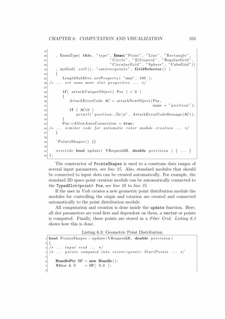
CHAPTER 6. COMPUTATION AND VISUALIZATION 103
19
20 , EnumType( this , ” type ” , Enum( ” Point ” , ” Line ” , ” Rectangle ” ,21 ” C i r c l e ” , ” E l l i s p o i d ” , ” RegularGrid ” ,22 ” Circu la rGr id ” , ” Sphere ” , ”CubeGrid” ) )23 , myGrid ( s e l f ( ) , ” e m i t t e r p o i n t s ” , GridSelector ( ) )24 25 LengthSubDivs . s e tProper ty ( ”max” , 100 ) ;26 /* . . . s e t some more s l o t p r o p e r t i e s . . . */27
28 i f ( attachUniqueObject ( Pos ) < 0 )29 30 AttachErrorCode AC = attachNewObject ( Pos ,31 name + ” p o s i t i o n ” ) ;32 i f ( AC<0 )33 p r i n t f ( ” p o s i t i o n : %s \n” , AttachErrorCodeMessage (AC) ) ;34 35 Pos−>AllowAutoConnection = true ;36 /* . . . s im i l a r code f o r automatic ro to r module c r ea t i on . . . */37 38
39 ˜ PointsShapes ( ) 40
41 o v e r r i d e bool update ( VRequest&R, double p r e c i s i o n ) . . . 42 ;
The constructor of PointsShapes is used to a constrain data ranges ofseveral input parameters, see line 25. Also, standard modules that shouldbe connected to input slots can be created automatically. For example, thestandard 3D space point creation module can be automatically connected tothe TypedSlot<point> Pos, see line 28 to line 35.
If the user in Vish creates a new geometric point distribution module themodules for controlling the origin and rotation are created and connectedautomatically to the point distribution module.
All computation and creation is done inside the update function. Here,all slot parameters are read first and dependent on them, a vector or pointsis computed. Finally, these points are stored in a Fiber Grid. Listing 6.3shows how this is done.
Listing 6.3: Geometric Point Distribution
1 bool PointsShapes : : update ( VRequest&R, double p r e c i s i o n )2 3 /* . . . input read . . . */4 /* . . . po in t s computed in t o vec tor<point> S ta r tPo in t s . . . */5
6 BundlePtr BP = new Bundle ( ) ;7 Slice & S = BP[ 0 .0 ] ;8

CHAPTER 6. COMPUTATION AND VISUALIZATION 104
9 string grid name = Name( ) + ” P o i n t D i s t r i b ” ;10 Grid & PointGrid = S . newGrid ( grid name ) ;11
12 Skeleton & PointVer t i c e s = PointGrid . makeVertices ( 3 ) ;13 RefPtr<Chart> myCartesian = PointGrid . makeChart (14 typeid ( CartesianChart3D ) ) ;15
16 Representation&C ar t e s i a nVe r t i c e s = Po in tVer t i c e s [ myCartesian ] ;17 RefPtr<Field> Coords = Ca r t e s i an Ver t i c e s [ FIBER POSITIONS ] ;18
19 typedef MemArray<1, point> CrdsA t ;20 RefPtr<CrdsA t> CoordsData = new CoordsArray t (21 Star tPo in t s . s i z e ( ) ) ;22
23 MultiArray<1,point > & Crds1 = *CoordsData ;24 25 for ( i ndex t i =0; i < Star tPo in t s . s i z e ( ) ; i++ )26 27 MultiIndex<1> n( i ) ;28 Crds1 [ n ] = Star tPo in t s [ i ] ;29 30 31 Coords−>s e tPe r s i s t en tData ( CoordsData ) ;32
33 GridSelector GS( grid name , BP ) ;34 myGrid << R << GS;35
During the development the idea arose to use a Fiber Grid object handleinstead of the Point3D attribute for defining the translation. A minor changein the point distribution module made it possible to create the shapes at allthe 3D points of the input grid. So every point of the Fiber Grid was anorigin to the created shape. Thus, complicated point distributions could becreated in a recursive fashion by combining more point distribution modulesone after the other.
For example, the first point distribution module would create a line ofpoints and output the Fiber Grid. A second point distribution module wouldtake this as an input grid and around each point of the line would create asmall circle of points.
Later this recursive creation functionality was identified to be a pureFiber Grid operation and was thus extracted into an own module onlyoperating on Fiber Grid objects. The operation was called Grid Convolu-tion and is described in detail in section 6.1.1.

CHAPTER 6. COMPUTATION AND VISUALIZATION 105
Figure 6.2: Vish network for drawing points of a geometric point distribu-tion. The modules PointDistributionrotation and Point3 create a point anda rotor which are input into the distribution module PointDistribution. Thedistribution module creates a Fiber Grid which is output into the module fordrawing the vertices.
Random Point Distribution
The random point distribution creates seed points in a certain volume whichare randomly placed in space. One parameter controls the number of pointsgenerated and one a random seed. There are two ways how the dimensionsof the volume can be controlled.
Firstly, a radius parameter can be used that specifies the length of a cubicvolume, see figure 6.3.
Secondly, a Fiber Grid object can be connected instead. The boundingbox of this objects then defines the size of the volume. If the Fiber Gridnests a Fiber Scalar Field it is possible to filter the created random pointsby a certain scalar value range. In that case, the scalar value is evaluatedat each random point and is checked against the given range. If the value isoutside the range, the point is clipped.
Figure 6.4 shows some clipped random points by clipping against thepressure value, revealing some structure of a mixing ventilator in the centerof the data set.
During the use of the clipping functionality it was recognized that thisfeature could be taken further and used in other aspects as well. Making itpossible to sample any given Fiber Field on an arbitrary other Fiber Grid

CHAPTER 6. COMPUTATION AND VISUALIZATION 106
Figure 6.3: Random point distribution in a volume controlled by the radiusparameter.
would open a range of new visualization possibilities in a very flexible way.For example, one could compute an isosurface, which is handled as a
Fiber Grid object, of a scalar field and sample a second scalar field onto theisosurface. Then, the values of the second scalar field could be visualizedvia a color map on the isosurface. So one could, for example, analyze atemperature on a zero pressure isosurface. First Steps implementing thea general field on grid evaluator module were started but still have to becompleted.
Listing 6.4 shows the class header of the random point distribution.It is a Vish Module by deriving from VObject. The class gets a FiberGrid handle and inherits functionality to extract all Fiber Grid informationby being derived from Fish<Fiber::Slice>, Fish<Fiber::Skeleton> andFish<Fiber::Grid>. To equip the module with an additional Fiber Fieldhandle (for the clipping scalar field) a TypedSlot<Fiber::Field> is addedas an attribute. Additionally the class is derived from StatusIndicator
which enables some string output inside the GUI of the module. The outputis a new Fiber Grid object which is stored in the Fiber Bundle of the inputgrid.
Listing 6.4: Random Point Distribution
1
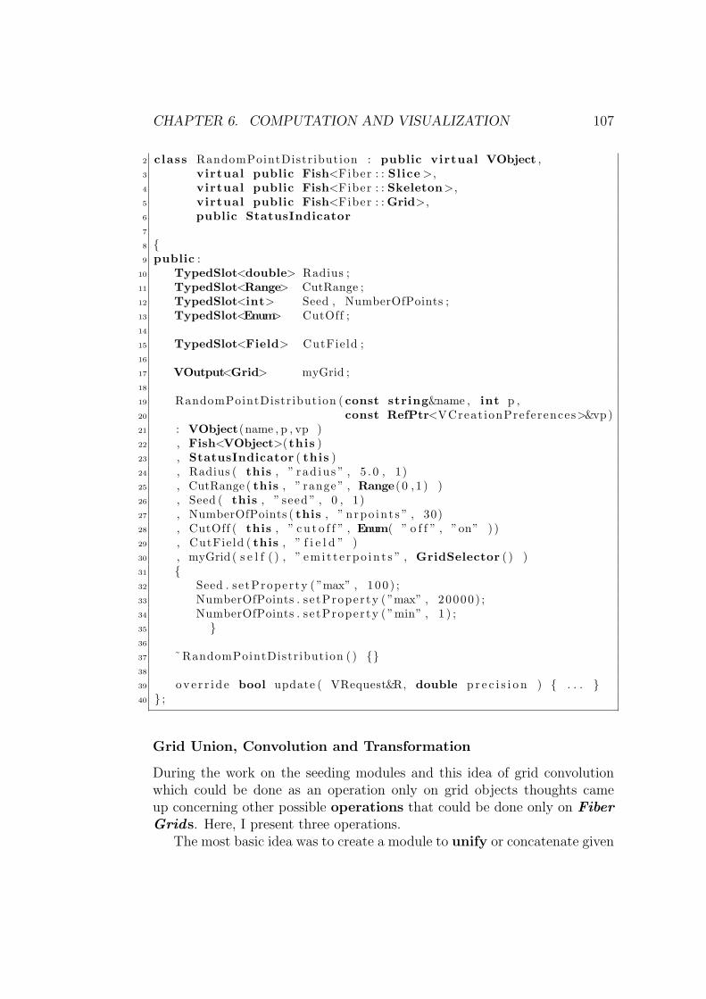
CHAPTER 6. COMPUTATION AND VISUALIZATION 107
2 class RandomPointDistribution : public virtual VObject ,3 virtual public Fish<Fiber : : Slice >,4 virtual public Fish<Fiber : : Skeleton>,5 virtual public Fish<Fiber : : Grid>,6 public StatusIndicator7
8 9 public :
10 TypedSlot<double> Radius ;11 TypedSlot<Range> CutRange ;12 TypedSlot<int> Seed , NumberOfPoints ;13 TypedSlot<Enum> CutOff ;14
15 TypedSlot<Field> CutField ;16
17 VOutput<Grid> myGrid ;18
19 RandomPointDistribution ( const string&name , int p ,20 const RefPtr<VCreat ionPreferences>&vp )21 : VObject(name , p , vp )22 , Fish<VObject>(this )23 , StatusIndicator ( this )24 , Radius ( this , ” rad iu s ” , 5 . 0 , 1)25 , CutRange ( this , ” range ” , Range( 0 , 1 ) )26 , Seed ( this , ” seed ” , 0 , 1)27 , NumberOfPoints ( this , ” n rpo in t s ” , 30)28 , CutOff ( this , ” c u t o f f ” , Enum( ” o f f ” , ”on” ) )29 , CutField ( this , ” f i e l d ” )30 , myGrid ( s e l f ( ) , ” e m i t t e r p o i n t s ” , GridSelector ( ) )31 32 Seed . se tProper ty ( ”max” , 1 0 0 ) ;33 NumberOfPoints . s e tProper ty ( ”max” , 20000) ;34 NumberOfPoints . s e tProper ty ( ”min” , 1 ) ;35 36
37 ˜ RandomPointDistribution ( ) 38
39 o v e r r i d e bool update ( VRequest&R, double p r e c i s i o n ) . . . 40 ;
Grid Union, Convolution and Transformation
During the work on the seeding modules and this idea of grid convolutionwhich could be done as an operation only on grid objects thoughts cameup concerning other possible operations that could be done only on FiberGrids. Here, I present three operations.
The most basic idea was to create a module to unify or concatenate given
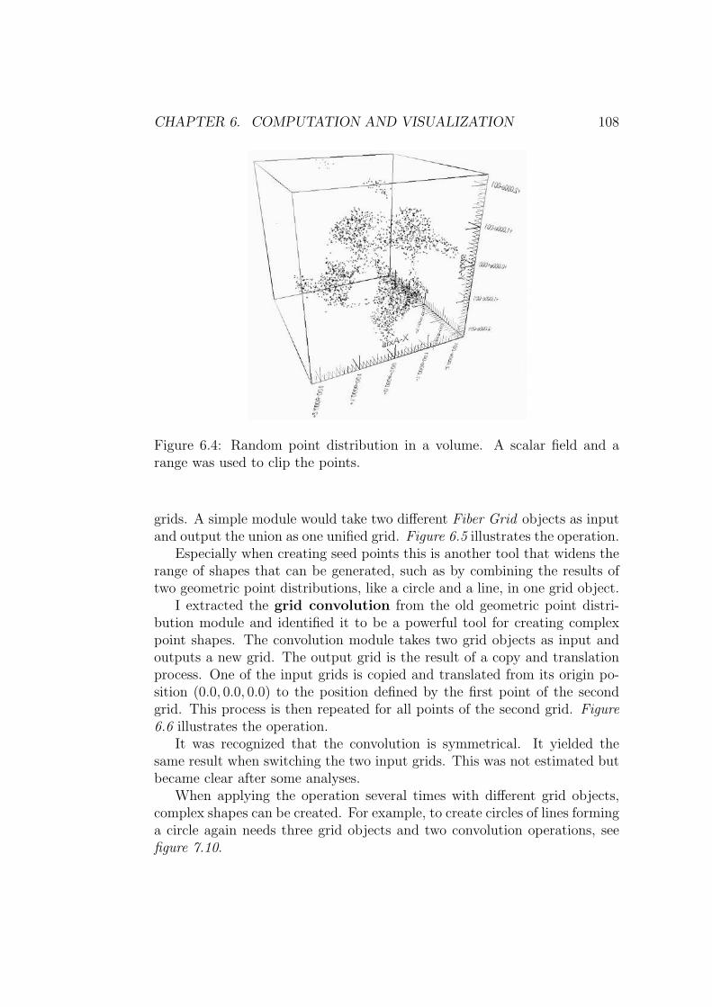
CHAPTER 6. COMPUTATION AND VISUALIZATION 108
Figure 6.4: Random point distribution in a volume. A scalar field and arange was used to clip the points.
grids. A simple module would take two different Fiber Grid objects as inputand output the union as one unified grid. Figure 6.5 illustrates the operation.
Especially when creating seed points this is another tool that widens therange of shapes that can be generated, such as by combining the results oftwo geometric point distributions, like a circle and a line, in one grid object.
I extracted the grid convolution from the old geometric point distri-bution module and identified it to be a powerful tool for creating complexpoint shapes. The convolution module takes two grid objects as input andoutputs a new grid. The output grid is the result of a copy and translationprocess. One of the input grids is copied and translated from its origin po-sition (0.0, 0.0, 0.0) to the position defined by the first point of the secondgrid. This process is then repeated for all points of the second grid. Figure6.6 illustrates the operation.
It was recognized that the convolution is symmetrical. It yielded thesame result when switching the two input grids. This was not estimated butbecame clear after some analyses.
When applying the operation several times with different grid objects,complex shapes can be created. For example, to create circles of lines forminga circle again needs three grid objects and two convolution operations, seefigure 7.10.
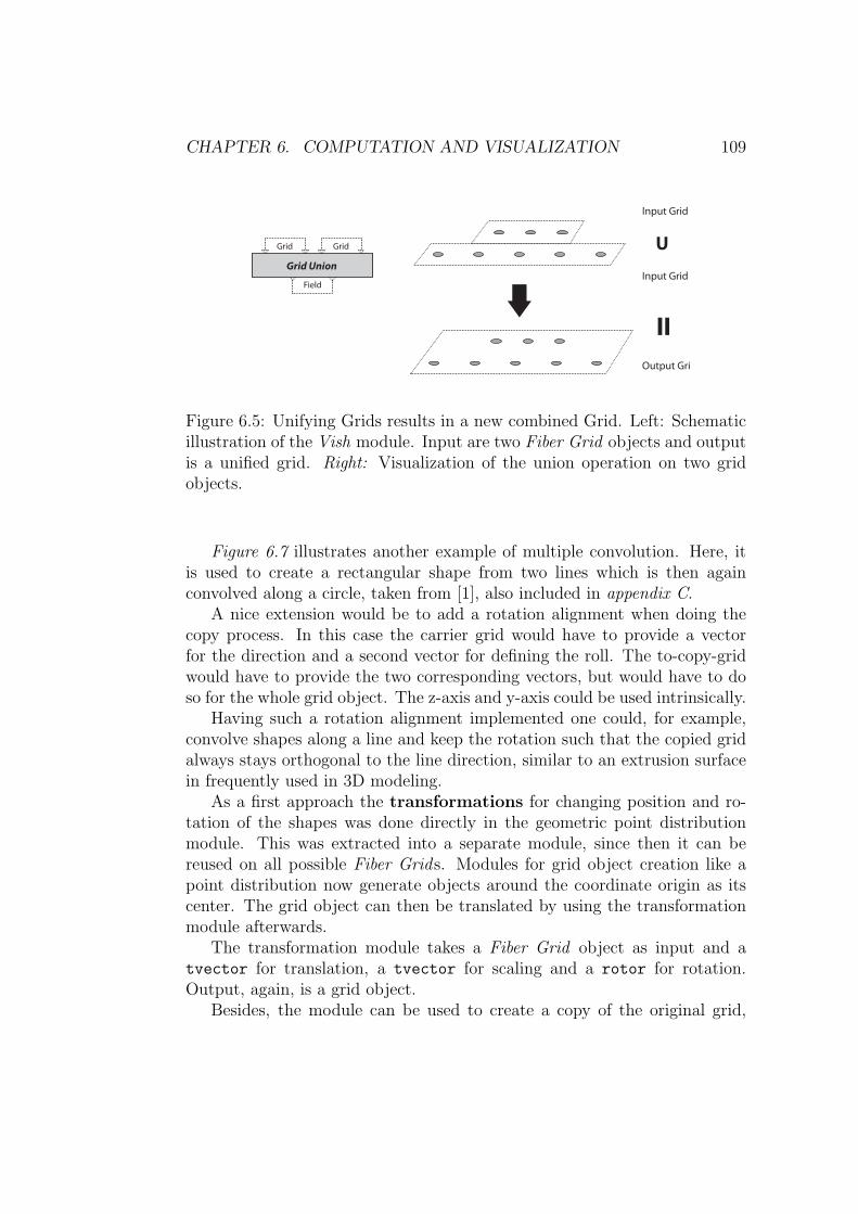
CHAPTER 6. COMPUTATION AND VISUALIZATION 109
Input Grid 1
Input Grid 2
Output Grid
Grid
Field
Grid Union
Grid U
Figure 6.5: Unifying Grids results in a new combined Grid. Left: Schematicillustration of the Vish module. Input are two Fiber Grid objects and outputis a unified grid. Right: Visualization of the union operation on two gridobjects.
Figure 6.7 illustrates another example of multiple convolution. Here, itis used to create a rectangular shape from two lines which is then againconvolved along a circle, taken from [1], also included in appendix C.
A nice extension would be to add a rotation alignment when doing thecopy process. In this case the carrier grid would have to provide a vectorfor the direction and a second vector for defining the roll. The to-copy-gridwould have to provide the two corresponding vectors, but would have to doso for the whole grid object. The z-axis and y-axis could be used intrinsically.
Having such a rotation alignment implemented one could, for example,convolve shapes along a line and keep the rotation such that the copied gridalways stays orthogonal to the line direction, similar to an extrusion surfacein frequently used in 3D modeling.
As a first approach the transformations for changing position and ro-tation of the shapes was done directly in the geometric point distributionmodule. This was extracted into a separate module, since then it can bereused on all possible Fiber Grids. Modules for grid object creation like apoint distribution now generate objects around the coordinate origin as itscenter. The grid object can then be translated by using the transformationmodule afterwards.
The transformation module takes a Fiber Grid object as input and atvector for translation, a tvector for scaling and a rotor for rotation.Output, again, is a grid object.
Besides, the module can be used to create a copy of the original grid,
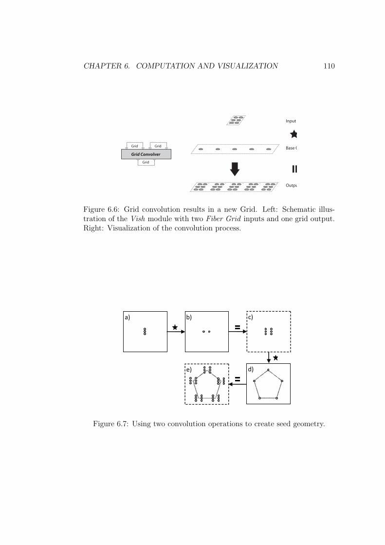
CHAPTER 6. COMPUTATION AND VISUALIZATION 110
Input Grid
Base Grid
Output Grid
Grid
Grid
Grid Convolver
Grid
Figure 6.6: Grid convolution results in a new Grid. Left: Schematic illus-tration of the Vish module with two Fiber Grid inputs and one grid output.Right: Visualization of the convolution process.
a) b) c)
d) e)
Figure 6.7: Using two convolution operations to create seed geometry.

CHAPTER 6. COMPUTATION AND VISUALIZATION 111
Figure 6.8: Seeding points created on a rectangular shape by a geometricpoint distribution module are transformed and copied several times by onegrid transformation module. Re-applied scaling and positing creates a pyra-mid grid.
and furthermore it allows multiple copies with re-applied transformations.For example, when the grid object is scaled by 1.2 in x-direction and threemultiple copies are generated, the copies have the scalings 1.2, 1.4 and 1.6.Similar rules apply to the other transformations, translation and rotation.
Thus, the module provides another basic tool to generate complex pointdistributions. Figure 6.8 shows multiple copies of a rectangle with the re-peated translation and scaling, forming now a whole pyramid.
6.1.2 Defining Initial Directions
To solve second-order differential equations, like the geodesic equation, itis necessary on top of this to specify an initial direction besides the initialposition. Using the Vish environment it develops naturally to define initialdirections as a Fiber Field of vectors on the Fiber Grid object used fordefining the initial positions.
Grid Subtraction
A direction vector is simply computed by a vector subtraction. This led tothe idea of defining the same operation on grid objects by subtracting allvertices of one grid from the vertices of the other grid. The computed FiberField is stored to the base grid, where the vectors are pointing from.
The following restriction applies to the module: The numbering of thevertices of the two grid objects must be compatible as well as the number ofvertices must be the same. Figure 6.9 illustrates the operation.

CHAPTER 6. COMPUTATION AND VISUALIZATION 112
Input Grid 1
Input Grid 2
Output Vector
Field
0 1 2 3 4
0 1 2 3 4 Grid
Field
Grid Subtractor
Grid
Figure 6.9: Subtracting grid objects results in a vector field. Left: Schematicillustration of the Vish module. Two Fiber Grid objects are input and oneFiber Field object is output. Right: Illustration of the subtraction. Con-sistent numbering of vertices in both grids is assumed as indicated by thenumber labels.
The module provides two parameters. One to enable the normalizationof the vectors and one for scaling the vectors by a scalar factor. Scaling isdone after normalization. So when normalize is yes and scale is 2.5, allvectors have a length of 2.5.
All of the presented modules were utilized to create the different kinds ofseeding geometries and vector fields for the visualizations shown in chapter7. For some seeding geometries up to five of the basic seeding modules werecombined.
For example, the tube-like seeding of figure 7.40 was created using twogeometric point distributions (a line and a circle) that were combined by agrid convolution, then copied and offset by a grid transformation and finallythese two grid were subtracted to yield the vector field for seeding the geodesiccomputation module.
6.2 Computation
The following section describes the computation and my implementation ofstreamlines and geodesics. The code structure was re-factored several times,finally yielding the geodesic module. Here, I describe the evolution processas it illustrates important key features of the current solution.
As mentioned in section 6.1.2, the whole task of the visualization is splitinto modules. Seeding points and directions are defined using Fiber Grid

CHAPTER 6. COMPUTATION AND VISUALIZATION 113
and Fiber Field objects. The first computation module I implemented was astreamline module. The input was a vector field describing the velocity of afluid and the seeding point.
The update function first did the data access on the Fiber Bundleinput objects. Then, a main loop solved the differential equation step-ping along each streamline after another. It used the get function ofLocalFromWorldPoint, see chp:interpol. Finally, a Fiber Grid objectof lines was output.
I recognized the advantage when adding more data to the line grid as FiberFields. This information was used for rendering and coloring the streamlinesin the rendering module. The interpolated vectors and the magnitude1 wereadded as fields to the line grid object. Later, all necessary information thatwould be needed to interpolate any other data field on the lines was addedas well. Local coordinates and fragment IDs were now also stored as fieldson the stream line grid.
Before implementing the module for geodesic computation the stream-line module was analyzed and several code parts were identified that werealso applicable to the geodesic module. Also other types of integral linescould reuse this code. Thus, I implemented a template base class for generalintegration lines. The parameters to control the computation are:
Input field
Input emitter grid (and field)
Line length
Step size
Type of solving the differential equation
Flags for adding additional Data
I implemented the template class IntegralLines over the two template pa-rameters FieldType and LineType. The FieldType specifies the type of thedata field that is used to compute the integral lines. In case of a stream-line it is a tvector for a vector field and in case of a stationary geodesicit is metric33 for the tensor field. The LineType is necessary since differ-ent integral lines may be computed on the same FieldType. For example,a path-line would have the same FieldType as a streamline but a differentLineType. The LineType is a Type Trait as described in section 3.1.
1Eukildean norm
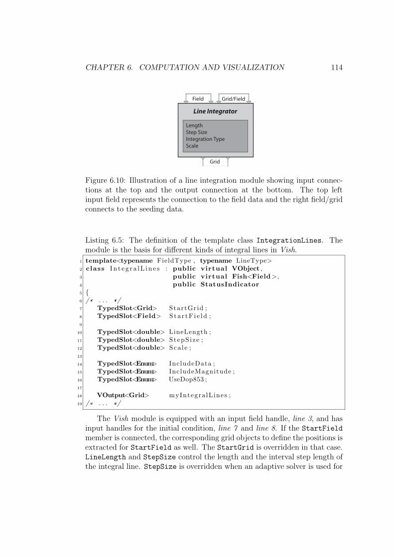
CHAPTER 6. COMPUTATION AND VISUALIZATION 114
Field Grid/Field
Grid
Line Integrator
LengthStep SizeIntegration TypeScale
Figure 6.10: Illustration of a line integration module showing input connec-tions at the top and the output connection at the bottom. The top leftinput field represents the connection to the field data and the right field/gridconnects to the seeding data.
Listing 6.5: The definition of the template class IntegrationLines. Themodule is the basis for different kinds of integral lines in Vish.
1 template<typename FieldType , typename LineType>2 class I n t e g r a l L i n e s : public virtual VObject ,3 public virtual Fish<Field>,4 public StatusIndicator5 6 /* . . . */7 TypedSlot<Grid> StartGr id ;8 TypedSlot<Field> S t a r t F i e l d ;9
10 TypedSlot<double> LineLength ;11 TypedSlot<double> StepS ize ;12 TypedSlot<double> Sca l e ;13
14 TypedSlot<Enum> IncludeData ;15 TypedSlot<Enum> IncludeMagnitude ;16 TypedSlot<Enum> UseDop853 ;17
18 VOutput<Grid> myIntegra lL ines ;19 /* . . . */
The Vish module is equipped with an input field handle, line 3, and hasinput handles for the initial condition, line 7 and line 8. If the StartField
member is connected, the corresponding grid objects to define the positions isextracted for StartField as well. The StartGrid is overridden in that case.LineLength and StepSize control the length and the interval step length ofthe integral line. StepSize is overridden when an adaptive solver is used for

CHAPTER 6. COMPUTATION AND VISUALIZATION 115
integration. The enumerations in line 13 and line 14 flag if additional datashould be stored as fields on the output grid. UseDop853 switches betweenfirst order Euler and adaptive 8th order Runge Kutta integration.
It follows an overview of the tasks done in the update function:
1. Get input field information
2. Get emitter grid or emitter field information
3. Create grid output name and check if re-computation is necessary
4. Create automatic seed points if no emitter grid is available
5. Do the integration
6. Bake a new Grid object that carries the actual lines
All these tasks are the same for streamlines and geodesics. Besides operatingon different types of data, the only task that has to be specialized for eachLineType is task 6, the actual integration.Task 1 and 2:The handles to the Fiber Grid and Fiber Field objects are extracted by usingGridSelector and FieldSelector as described in section 5.2.2Task 3:Here it is checked if an output grid is already existent from an earlier compu-tation. Since the line grid object is stored in the Fiber Bundle it can be triedto get such a grid from the bundle, see line 4 in listing 6.6. If no valid gridis returned a new one has to be computed. Otherwise it is checked whetherthe input field, the line length, the step size, the connection to the input fieldand the emitter grid are older than the coordinate field of the output grid.If they all are older a return exits the update function of the module. Ifone of these objects is younger than the found grid at the output it has tobe recomputed.
Listing 6.6: Source code that checks if the integration line grid at the outputhas to be recomputed because of changes of the input field, the seed pointgrid or module parameters.
1 string grid name = F i e l d S e l e c t i o n . Gridname ( ) + ” ” + Name ( ) ;2
3 Info< Fiber : : Slice > A c t u a l S l i c e = F i e l d S e l e c t i o n . F ie ldSource ;4 RefPtr<Grid> OutGrid = (* A c t u a l S l i c e . second ) ( grid name ) ;5
6 i f ( OutGrid )7

CHAPTER 6. COMPUTATION AND VISUALIZATION 116
8 i f (RefPtr<Field> OutCrds = OutGrid−>g e t C a r t e s i a n P o s i t i o n s ( ) )9
10 i f ( InputToIntegrateF ie ld −>isOlderThan ( *OutCrds ) &&11 LineLength−>age ( Context ) . isOlderThan ( *OutCrds ) &&12 StepS ize −>age ( Context ) . isOlderThan ( *OutCrds ) &&13 ConnectionAge ( ) . isOlderThan ( *OutCrds ) )14 15 i f ( EmitterCoordinates )16 17 i f ( EmitterCoordinates−>isOlderThan ( *OutCrds ) )18 return s e t S t a t u s I n f o ( Context ,19 ” Reusing prev ious computation ” ) ;20 21 else22 return s e t S t a t u s I n f o ( Context ,23 ” Reusing prev ious computation ( no emit t e r ) ” ) ;24
To equip a class with the aging functionality one derives it from theMemcore::Ageable base class of the Vish environment. Field and Grid arederived from Agable and can be compared to other ageable objects, see line10 and line 17. The TypedSlot has an age as a member. Here, the Context
on which parameters depend is important, see line 11 and line 12.Task 4:If no emitter grid or emitter field is found a new emitter grid is created. Thepositions of the seed points are then created along a diagonal of the boundingbox of the connected input data field.Task 5:The main loop uses a Type Trait2 class for integration, see listing 6.7 line 1.The integrator has to be initialized by a handle to a container storing thecomputed lines, a handle to a data field, a LocalPointFinder, the step sizefor one integration step, a flag for the integration type, the number of stepsand the time when the integration is started.
Listing 6.7: Main loop
1 Line Integra to r <FieldType , LineType> I n t e g r a t o r (2 Lines , F i e l d S e l e c t i o n ,3 LocalPointFinder ,4 s t e p s i z e , Dop ( ) ,5 l i n e l e n g t h , time ) ;6 int s t ep count e r = 0 ;7
8 while ( h a s f i n i s h e d == fa l se && step counte r < l i n e l e n g t h )9
2section 3.1

CHAPTER 6. COMPUTATION AND VISUALIZATION 117
10 /* . . . */11 h a s f i n i s h e d = MyLineIntegrator . advanceBreadthFirst ( ) ;12 s t ep count e r++;13
The LineIntegrator template can be specialized if necessary. Forstreamlines and geodesics this was not required and the general templatedefinition was sufficient. Calling the integrateBreadthFirst function, line1, advances all integral lines by one integration step. This is repeated untilthe LineLength is reached or all lines cannot be computed further, line 8.
1 template<class FieldType , typename LineType>2 class L i ne I n t e g ra to r3 4 /* . . . */5 AtomicIntegrator<FieldType , LineType> AI ;6 /* . . . */7
8 bool advanceBreadthFirst ( )9
10 unsigned end counter = 0 ;11
12 i f ( dop )13 AI . initDop853 ( Lines . s i z e ( ) ) ;14
15 for (unsigned p = 0 ; p < Lines . s i z e ( ) ; p++)16 17 /* . . . */18 i f ( ! dop )19 t e s t = AI . doEuler ( * In t eg ra t i onL ine , time ) ;20 else21 t e s t = AI . doDop853 ( * In t eg ra t i onL ine , time , p ) ;22 /* . . . */23 24 return ( end counter == Lines . s i z e ( ) ) ? true : fa l se ;25 26 ;
The LineIntegrator uses an instance of the AtomIntegrator to computethe integration steps, see line 5. The AtomIntegrator is a Type Trait asdescribed in section 3.1 and has to be specialized and implemented for eachkind of integration line. The loop in line 10 iterates over all integration linesof the Line container and advances each line by one step. If all lines cannotbe computed further, for example because they have stepped outside the datafield domain, advanceBreadthFirst returns true, otherwise false.Task 6:Now the computed lines have to be stored as a Fiber Grid object into the

CHAPTER 6. COMPUTATION AND VISUALIZATION 118
<class FieldType, class LineType>LineIntegrator
bool advanceBreadFirst()
<class FieldType, class LineType>AtomicIntegrator
bool doEuler( ... )void initDop853(...)bool doDop853(...)
AtomicDataBase
GeodesicIntegrator
bool doEuler( ... )void initDop853(...)bool doDop853(...)
<class FieldType, class LineType>IntegralLine
override bool update( ... )
VObject
StatusIndicator
<class FiberType>Fish
<Field>
<class FieldType, class LineType>IntegralLine
bool update( ... )
Type Trait
Figure 6.11: UML diagram of class relationships for integral lines. The Vishmodule IntegralLines uses a reference of LineIntegrator in the updatefunction. The LineIntegrator, finally, uses a reference of the Type TraitAtomicIntegrator doing the integration. An AtomicDataBase is providedto equip the AtomicIntegrator with data structures needed for computationwhich are initialized by the LineIntegrator.
Fiber Bundle. Here, it is illustrated how the vertices, the connectivity andthe interpolated field data of the lines are stored. For a more detaileddescription like storing other fields on the grid, chapter 4. First, a new FiberGrid object is prepared to be added to the Fiber Bundle of the input datafield for storing the lines:
1 RefPtr<Grid> In t eg ra lL ineGr id =2 F i e l d S e l e c t i o n . theSourceBundle−>newGrid ( ) ;3 Grid&LineGrid = * In t eg ra lL ineGr id ;
Creating the IntegralLineGrid using the newGrid function does not addthe grid to the Fiber Bundle. The grid is added later, when the data hasbeen baked completely. The pointer to the bundle is extracted from theFieldSelector of the input data field. Thus, the grid will be added into thebundle hosting the input data field.
Next, a new Fiber Field is created to store the vertex data of the integrallines:
1 RefPtr<Field> L inePos i t i on s = new Field ( ) ;2
3 RefPtr<MemArray<1, point> > Pts = new MemArray<1,point>(4 MIndex ( nPoints ) ) ;

CHAPTER 6. COMPUTATION AND VISUALIZATION 119
5
6 RefPtr<Chunk<point> > data = Pts−>myChunk ( ) ;7 std : : vector<point>&LineCoordinates = data−>s t d v e c t o r ( ) ;8
9 i ndex t Pt = 0 ;10
11 /* loop , s t o r e po in t s in 1D Array LineCoordinates */12 LineCoordinates [ Pt ] = ( PointsPerLine [ ver ] ) . l o c a t i o n ;13 Pt++;14 /* . . . */15 LinePos i t i ons−>s e tPe r s i s t en tData ( Pts ) ;
After creating a 1D MemArray of the correct size, line 1, its data access us-ing a std::vector is prepared (line 6 and line 7 ). All vertices are then storedsequentially in the MemArray, line 12. The Fiber Field ’s setPersistantDatafunction stores the data into the Field, line 15. Using this function ensuresthat data is always kept in memory for caching. Here, room for improvementremains. A more sophisticated mechanism might be appropriate.
The created data field of the vertex is now added to the grid objectLineGrid:
1 Skeleton&LineVer t i c e s = LineGrid . makeVertices ( 3 ) ;2 RefPtr<Chart> myCartesian = LineGrid . makeChart (3 typeid ( Fiber : : CartesianChart3D ) ) ;4 Representation&Vert i c e sAsCarte s ian = LineVer t i c e s [ myCartesian ] ;5 Vert i c e sAsCarte s ian . s e t P o s i t i o n s ( L inePos i t i on s ) ;
Since the field describes the vertices of the grid a skeleton of vertices is cre-ated, line 1, the vertices being represented in Cartesian coordinates. Thus, acorresponding Chart object is generated and used to create a Coordinaterepresentation. Finally, the Fiber Field LinePositions is added to thegrid by calling setPosition on the representation passing the field. ThemakeVertices function is used for convenience substituting the creation ofa skeleton of 0 dimensionality and 0 index depth, chapter 4.
Next, the connectivity of the vertices is stored:
1 typedef MemArray<1, std : : vector<index t > > EdgesArray t ;2 Ref<EdgesArray t> EdgesArray ( NumberOfLines ) ;3 MultiArray<1, std : : vector<index t > >&Edges = *EdgesArray ;4 i ndex t ve r t count ;5
6 /* l oop over number o f l i n e s */7 ver t count = 08 /* l oop over v e r t i c e s in one l i n e */9 Edges [ l i n e ] [ ver ] = ver t count ;
10 ver t count++;11

CHAPTER 6. COMPUTATION AND VISUALIZATION 120
12 Skeleton&LineEdges = LineGrid [ SkeletonID (1 , 1 ) ] ;13 Representation&EdgesAsVert ices = LineEdges [ L ineVer t i c e s ] ;14 EdgesAsVert ices . s e t P o s i t i o n s ( new Field ( EdgesArray ) ) ;
The connectivity is stored as a sequence of indices for each line running from0 to the length of the line minus 1. The skeleton to describe an edge has adimensionality of 1, since an edge is a one dimensional object, and an indexdepth of 1 since it requires one lookup to get to a vertex position, line 12.The representation is on the line’s vertices, line 13. Finally a new data fieldholding the edge data is created and added to the grid in line 14.
This is an example of storing data on the vertices where data is of templatetype Fieldtype:
1 typedef MemArray<1, FieldType> LinesDataArr t ;2 Ref<LinesDataArr t> LinesData ( nPoints ) ;3 MultiArray<1,FieldType>&LineData = *LinesData ;4 i ndex t ve r t count = 0 ;5
6 /* l oop over v e r t i c e s */7 LineData [ MIndex ( ve r t count ) ] = Line [ ver ] . data ;8 ver t count++;9
10 Vert i c e sAsCarte s ian [ Fieldname ( Context ) ]−>11 s e tPe r s i s t en tData ( LinesData ) ;12 Vert i c e sAsCarte s ian [ TangentialVectorFieldName ]−>13 s e tPe r s i s t en tData ( LinesData ) ;
Data is stored in the same layout as the vertices. The same representationVerticesAsCartesian is used specifying a name to identify the data field.More than one name used. The data field is not created twice in the bundle,just an alternative name ist stored.
Finally the baked Fiber Grid is inserted into the bundle at a certain FiberSlice:
1 c u r r e n t S l i c e . g e t S l i c e ()−> i n s e r t ( grid name , In t eg ra lL ineGr id ) ;2 GridSelector GS( grid name , F i e l d S e l e c t i o n . BundleSource ( ) ) ;3 myIntegra lL ines << Context << GS
Also, the a handle to the line grid is output at the VOutput of the integrationline module.
Next is the description of computation and implementation of stream-lines and geodesics. Other integral lines can also be based on the providedIntegralLines template classes: Implementing pathlines in vector fields orgradient lines in gradient or scalar fields is straightforward with a minimaleffort in producing lines of code.

CHAPTER 6. COMPUTATION AND VISUALIZATION 121
0 12
3
4
Figure 6.12: Computing a streamline in a vector field describing the velocityof a fluid. Starting at an initial position and following the direction of thevector field by a certain step size solves the differential equation defining thestreamline curve.
6.2.1 Computing First Order Integration Lines
As described in section 2.3 streamlines are a common tool to visualize flowin fluid dynamics. Streamlines are integral lines of first order, see equation(2.75).
To solve the equation I first implemented a simple explicit Euler integra-tion scheme. At the initial position the local coordinates of the vector fieldare computed. These are then used to compute the vector at that positionby linear interpolation of the vector field.
According to equation (2.75), the vector at that position is equal to thederivative of the streamline. A new point of the streamline can now becomputed by stepping into the direction of the vector. The step size iscontrolled by the user. Figure 6.12 illustrates the process. Computationstarts at point 0 and continues following the vector field.
Implementation is done by specializing the AtomicIntegrator class pro-vided by the integral architecture. A new type trait, the streamline, has tobe introduced as well:
Listing 6.8: Layout of the streamline specialization of AtomicIntegrator.
1 struct Streaml ine ;2
3 template<>4 class AtomicIntegrator<tvector , Streamline >:public AtomicDataBase5 6 std : : vector<dop853<Tangent i a lD i f f e r en t i a lEquat i onL inea r >>Line In t s ;7 /* . . . */8

CHAPTER 6. COMPUTATION AND VISUALIZATION 122
9 bool doEuler ( std : : vector<In teg ra t i onPo int <tvector> >&IntLine ,10 const double&time ) ;11
12 bool in itDop853 ( const int number o f l i n e s ) ;13
14 bool doDop853 ( std : : vector<In teg ra t i onPo int <tvector> >&IntLine ,15 const double&time , const unsigned l i n e n r ) ;16 ;
The doEuler function finally implements the integration in a few lines ofsource code. Here follows the main part:
Listing 6.9: Excerpt of doEuler for streamlines.
1 bool t e s t=LocalPointFinder−>get ( IntL ine [ l a s t i n d e x ] . l o ca t i on ,2 l o c a l P o i n t ) ;3 /* . . . */4 IntL ine [ l a s t i n d e x ] . setData ( InterpolData , f l o a t i n d e x ,5 FragName ) ;6
7 Interpolate <3, tvector , L inear Ipo l <tvector> >8 myField ( *ToIntArr , l o c a l P o i n t . f i r s t ) ;9
10 tvector d i r = myField . eva l ( ) ;11
12 NewPoint = IntL ine [ l a s t i n d e x ] . l o c a t i o n + s t e p s i z e * d i r ;13 /* . . . */
First the local point coordinates are computed using the get function asdescribed in section 5.4. Then the vector is computed using interpolationtemplate classes provided by Vish. Finally the Euler step is done in line 12.The new point is then stored on the integration line, which is the basis forthe computation of the next step. One line is represented by a vector ofIntegrationPoints, which is a simple template container class to collect allinformation computed at one point of the integration line, here: point worldcoordinates, the interpolated data (vector), the local coordinates, the id ofthe multi-block.
The Euler method is fast if high accuracy of the solution is not important.To achieve high accuracy one has to use a very small step size for integration.
“We have studied its convergence extensively in Section 1.7 and have seenthat the global error behaves like Ch, where C is a constant depending onthe problem and h is the maximal step size. If one wants a precision of, say,6 decimals, one would thus need about a million steps, which is not verysatisfactory. ...” [34]
Runge-Kutta (RK) methods are based on Euler steps. More than oneEuler step is done and then combined into one RK step by several coefficients
CHAPTER 6. COMPUTATION AND VISUALIZATION 123
[34]:Let s be an integer (the ”number of stages”) and a21, a31, a32, ..., as1, as2,
..., as,s−1, b1, ..., bs, c2, ..., cs be real coefficients. Then the method
k1 = f(x0, y0) (6.1)
k2 = f(x0 + c2h, y0 + ha21k1)
k3 = f(x0 + c3h, y0 + h(a31k1 + a32k2)
...
ks = f(x0 + csh, y0 + h(as1k1 + ...+ as,s−1ks − 1)
y1 = y0 + h · (b1k1 + ...+ bsks)
is called an s-stage explicit Runge-Kutta method (ERK) for (1.1).Usually, the ci satisfy the conditions ...
ci =i−1∑j=1
aij. (6.2)
Such a method converges much faster to the correct solution. Whenchoosing the coefficient thoughtfully the error decreases exponentially:
||y(x0 + h)− y1||︸ ︷︷ ︸ <= Khp+1,
localerror(6.3)
with p denoting the order of the RK scheme. A famous example for coeffi-cients is “the” Runge-Kutta method of order 4. The coefficients are usuallygiven in tabular form:
0c2 a21
c3 a31 a32...
......
cs as1 as2 ... as,s−1
b1 b2 ... bs−1 bs
01/2 1/21/2 0 1/21 0 0 1
1/6 2/6 2/6 1/6
This is a 4 stage RK method and thus needs 4 evaluations of the function todo one integration step which, in case of the streamlines, requires computinglocal coordinates and doing the interpolation 4 times. Since the local errorbound decreases exponentially with the order, the step size can be increasedand, thus, much fewer total steps are needed for integration compared tosimple Euler integration.
Usually the analytically correct solution of a function is not known andlocal errors cannot be computed correctly. Nonetheless, a local error can be
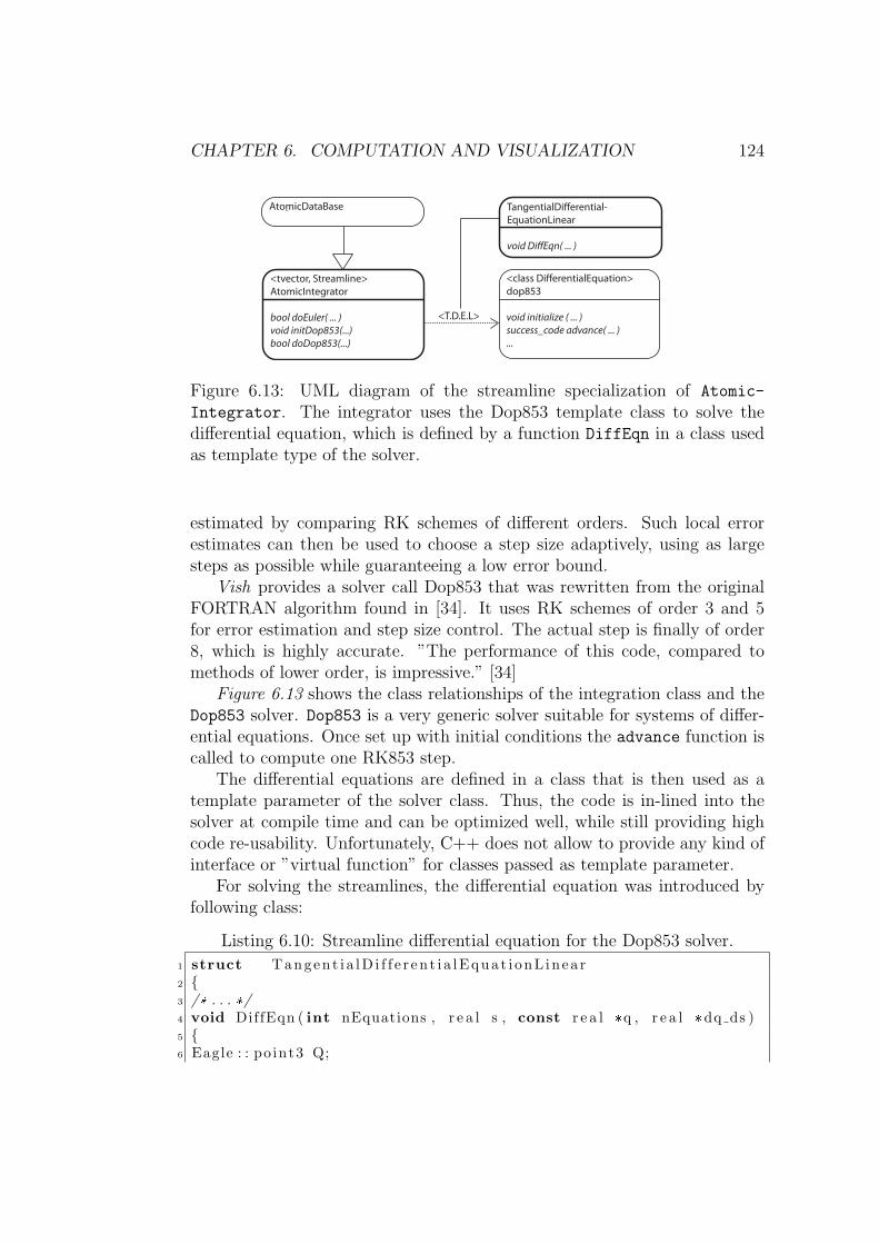
CHAPTER 6. COMPUTATION AND VISUALIZATION 124
<tvector, Streamline>AtomicIntegrator
bool doEuler( ... )void initDop853(...)bool doDop853(...)
AtomicDataBase TangentialDierential-EquationLinear
void DiEqn( ... )
<class DierentialEquation>dop853
void initialize ( ... ) success_code advance( ... )...
<T.D.E.L>
Figure 6.13: UML diagram of the streamline specialization of Atomic-
Integrator. The integrator uses the Dop853 template class to solve thedifferential equation, which is defined by a function DiffEqn in a class usedas template type of the solver.
estimated by comparing RK schemes of different orders. Such local errorestimates can then be used to choose a step size adaptively, using as largesteps as possible while guaranteeing a low error bound.
Vish provides a solver call Dop853 that was rewritten from the originalFORTRAN algorithm found in [34]. It uses RK schemes of order 3 and 5for error estimation and step size control. The actual step is finally of order8, which is highly accurate. ”The performance of this code, compared tomethods of lower order, is impressive.” [34]
Figure 6.13 shows the class relationships of the integration class and theDop853 solver. Dop853 is a very generic solver suitable for systems of differ-ential equations. Once set up with initial conditions the advance function iscalled to compute one RK853 step.
The differential equations are defined in a class that is then used as atemplate parameter of the solver class. Thus, the code is in-lined into thesolver at compile time and can be optimized well, while still providing highcode re-usability. Unfortunately, C++ does not allow to provide any kind ofinterface or ”virtual function” for classes passed as template parameter.
For solving the streamlines, the differential equation was introduced byfollowing class:
Listing 6.10: Streamline differential equation for the Dop853 solver.
1 struct T a n g e n t i a l D i f f e r e n t i a l E q u a t i o n L i n e a r2 3 /* . . . */4 void DiffEqn ( int nEquations , r e a l s , const r e a l *q , r e a l *dq ds )5 6 Eagle : : po int3 Q;
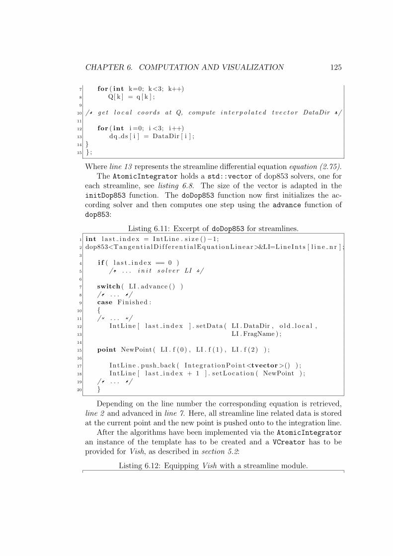
CHAPTER 6. COMPUTATION AND VISUALIZATION 125
7 for ( int k=0; k<3; k++)8 Q[ k ] = q [ k ] ;9
10 /* ge t l o c a l coords at Q, compute i n t e r p o l a t e d t v e c t o r DataDir */11
12 for ( int i =0; i <3; i++)13 dq ds [ i ] = DataDir [ i ] ;14 15 ;
Where line 13 represents the streamline differential equation equation (2.75).The AtomicIntegrator holds a std::vector of dop853 solvers, one for
each streamline, see listing 6.8. The size of the vector is adapted in theinitDop853 function. The doDop853 function now first initializes the ac-cording solver and then computes one step using the advance function ofdop853:
Listing 6.11: Excerpt of doDop853 for streamlines.
1 int l a s t i n d e x = IntL ine . s i z e ()−1;2 dop853<Tangent i a lD i f f e r en t i a lEquat i onL inea r >&LI=Line In t s [ l i n e n r ] ;3
4 i f ( l a s t i n d e x == 0 )5 /* . . . i n i t s o l v e r LI */6
7 switch ( LI . advance ( ) )8 /* . . . */9 case Fin i shed :
10 11 /* . . . */12 IntL ine [ l a s t i n d e x ] . setData ( LI . DataDir , o l d l o c a l ,13 LI . FragName ) ;14
15 point NewPoint ( LI . f ( 0 ) , LI . f ( 1 ) , LI . f ( 2 ) ) ;16
17 IntL ine . push back ( Integra t i onPo int <tvector >() ) ;18 IntL ine [ l a s t i n d e x + 1 ] . s e tLocat i on ( NewPoint ) ;19 /* . . . */20
Depending on the line number the corresponding equation is retrieved,line 2 and advanced in line 7. Here, all streamline line related data is storedat the current point and the new point is pushed onto to the integration line.
After the algorithms have been implemented via the AtomicIntegrator
an instance of the template has to be created and a VCreator has to beprovided for Vish, as described in section 5.2:
Listing 6.12: Equipping Vish with a streamline module.
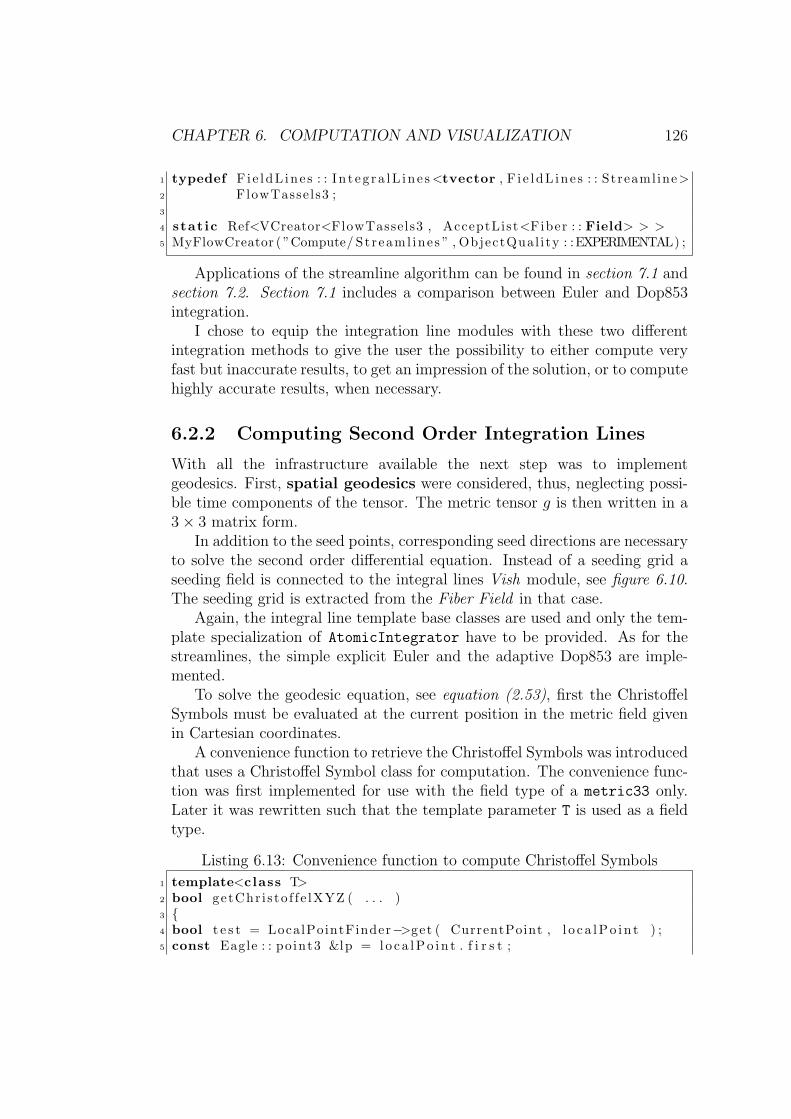
CHAPTER 6. COMPUTATION AND VISUALIZATION 126
1 typedef Fie ldL ine s : : I n t eg r a l L i n e s <tvector , F i e l dL ine s : : Streamline>2 FlowTasse ls3 ;3
4 stat ic Ref<VCreator<FlowTassels3 , AcceptList<Fiber : : Field> > >5 MyFlowCreator ( ”Compute/ St reaml ine s ” , ObjectQual i ty : :EXPERIMENTAL) ;
Applications of the streamline algorithm can be found in section 7.1 andsection 7.2. Section 7.1 includes a comparison between Euler and Dop853integration.
I chose to equip the integration line modules with these two differentintegration methods to give the user the possibility to either compute veryfast but inaccurate results, to get an impression of the solution, or to computehighly accurate results, when necessary.
6.2.2 Computing Second Order Integration Lines
With all the infrastructure available the next step was to implementgeodesics. First, spatial geodesics were considered, thus, neglecting possi-ble time components of the tensor. The metric tensor g is then written in a3× 3 matrix form.
In addition to the seed points, corresponding seed directions are necessaryto solve the second order differential equation. Instead of a seeding grid aseeding field is connected to the integral lines Vish module, see figure 6.10.The seeding grid is extracted from the Fiber Field in that case.
Again, the integral line template base classes are used and only the tem-plate specialization of AtomicIntegrator have to be provided. As for thestreamlines, the simple explicit Euler and the adaptive Dop853 are imple-mented.
To solve the geodesic equation, see equation (2.53), first the ChristoffelSymbols must be evaluated at the current position in the metric field givenin Cartesian coordinates.
A convenience function to retrieve the Christoffel Symbols was introducedthat uses a Christoffel Symbol class for computation. The convenience func-tion was first implemented for use with the field type of a metric33 only.Later it was rewritten such that the template parameter T is used as a fieldtype.
Listing 6.13: Convenience function to compute Christoffel Symbols
1 template<class T>2 bool getChr i s to f f e lXYZ ( . . . )3 4 bool t e s t = LocalPointFinder−>get ( CurrentPoint , l o c a l P o i n t ) ;5 const Eagle : : po int3 &lp = l o c a l P o i n t . f i r s t ;

CHAPTER 6. COMPUTATION AND VISUALIZATION 127
6 /* . . . */7
8 T g , g x , g y , g z ;9
10 Interpolate <3, T, CubicIpol<T> > myField ( *ToIntArr0 , lp ) ;11 g = myField . eva l ( ) ;12
13 RefPtr<Fiber : : Field> f i e l d=F i e l d S e l e c t i o n . g e t C a r t e s i a n P o s i t i o n s ( ) ;14 RefPtr<Fiber : : DirectProductMemArray<Eagle : : point3 ,3> >15 FData = f i e l d −>getData ( ) ;16
17 Eagle : : po int3 d e l t a = FData−>Delta ( ) ;18
19 Interpolate <3, T, CubicIpol<T>, double ,20 NoDelimiter<T>, 0 > myField x ( *ToIntArr0 , lp ) ;21 g x = myField x . eva l ( ) ;22
23 g x /= d e l t a [ 0 ] ;24
25 /* . . . s im i l a r f o r y and z . . . */26
27 C h r i s t o f f e l s = new Christo f fe lXYZ ( g , g x , g y , g z ) ;28
29 /* . . . */30
The getChristoffel function computes the local point using theLocalPointFinder, see section 5.4, which is then used to do a cubic in-terpolation of the metric tensor field, line 10. Vish’s interpolation classesalso can deliver derivatives. Line 19 illustrates how this is done. The lasttemplate parameter of interpolate specifies the axis direction of the deriva-tion (x direction is index 0). The derivative is computed in index coordinatesand thus has to be normalized by the interval length. Therefore, the intervaldistance is retrieved in line 17. A direct product array is utilized. By now,this technique is limited to uniform grids. For supporting other grid typesthe code between line 13 and line 26 has to be extended.
The ChristoffelXYZ class stores the metric tensor and its x, y and zderivatives and provides an operator to compute a component on demand:
Listing 6.14: Operator of ChristoffelXYZ to compute Christoffel Symbolson demand.
1 const double operator ( ) ( const unsigned mu,2 const unsigned nu ,3 const unsigned lambda ) const4 5 double gamma = 0 . 0 ;
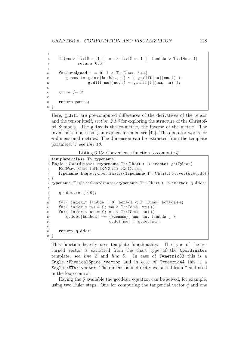
CHAPTER 6. COMPUTATION AND VISUALIZATION 128
6
7 i f (mu > T : : Dims−1 | | nu > T : : Dims−1 | | lambda > T : : Dims−1)8 return 0 . 0 ;9
10 for (unsigned i = 0 ; i < T : : Dims ; i++)11 gamma += g inv ( lambda , i ) * ( g d i f f [ nu ] (mu, i ) +12 g d i f f [mu] ( nu , i ) − g d i f f [ i ] (mu, nu) ) ;13
14 gamma /= 2 ;15
16 return gamma;17
Here, g diff are pre-computed differences of the derivatives of the tensorand the tensor itself, section 2.1.7 for exploring the structure of the Christof-fel Symbols. The g inv is the co-metric, the inverse of the metric. Theinversion is done using an explicit formula, see [42]. The operator works forn-dimensional metrics. The dimension can be extracted from the templateparameter T, see line 10.
Listing 6.15: Convenience function to compute q.
1 template<class T> typename2 Eagle : : Coordinates <typename T : : Chart t > : :vector getQddot (3 RefPtr< Christof fe lXYZ<T> >& Gamma,4 typename Eagle : : Coordinates<typename T : : Chart t > : : vector&q dot )5 6 typename Eagle : : Coordinates<typename T : : Chart t > : :vector q ddot ;7
8 q ddot . s e t ( 0 . 0 ) ;9
10 for ( i ndex t lambda = 0 ; lambda < T : : Dims ; lambda++)11 for ( i ndex t mu = 0 ; mu < T : : Dims ; mu++)12 for ( i ndex t nu = 0 ; nu < T : : Dims ; nu++)13 q ddot [ lambda ] −= (*Gamma) ( mu, nu , lambda ) *
14 q dot [mu] * q dot [ nu ] ;15
16 return q ddot ;17
This function heavily uses template functionality. The type of the re-turned vector is extracted from the chart type of the Coordinates
template, see line 2 and line 5. In case of T=metric33 this is aEagle::PhysicalSpace::vector and in case of T=metric44 this is aEagle::STA::vector. The dimension is directly extracted from T and usedin the loop control.
Having the q available the geodesic equation can be solved, for example,using two Euler steps. One for computing the tangential vector q and one

CHAPTER 6. COMPUTATION AND VISUALIZATION 129
for computing the next point x of the line. x0 and q0 must be given as initialconditions:
qi+1 = qi + hqixi+1 = xi + hqi+1
(6.4)
The Euler is implemented in the doEuler function of theAtomicIntegrator which is only partially template-specialized:
Listing 6.16: Layout of the partial geodesic specialization ofAtomicIntegrator, compare listing 6.8.
1 struct Geodesic ;2
3 template<>4 class AtomicIntegrator<T, Geodesic >:public AtomicDataBase5 6 typedef Traum : : dop853<Geode s i cD i f f e r en t i a lEquat i on <T>>D i f f S o l v e r ;7 typedef typename T : : Chart t Chart t ;8 typedef typename Coordinates<Chart t > : : point point ;9 typedef typename Coordinates<Chart t > : : vector tvector ;
10
11 std : : vector< D i f f S o l v e r > L i n e I n t e g r a t o r s ;12 /* . . . */13
14 bool doEuler ( std : : vector<In teg ra t i onPo int <T> >&IntLine ,15 const double&time ) ;16
17 bool in itDop853 ( const int number o f l i n e s ) ;18
19 bool doDop853 ( std : : vector<In teg ra t i onPo int <T> >&IntLine ,20 const double&time , const unsigned l i n e n r ) ;21 ;
The data field type is still a template parameter. Via the chart of the tem-plate type local typedefs define a point and tvector.
The doEuler function utilizes the convenience functions for the compu-tation of the Christoffel symbols and q.
Listing 6.17: Excerpt of doEuler for geodesics.
1 /* . . . */2 RefPtr<Christof fe lXYZ<T> > Gamma;3 T g cur r ;4 pair<Eagle : : Phys ica lSpace : : point , string>l o c a l P o i n t ;5
6 bool t e s t = F i e ldL ine s : : getChr i sto f fe lXYZ<T>( P curr ,7 LocalPointFinder , F i e l d S e l e c t i o n , s t e p s i z e ,8 Gamma, g curr , l o c a l P o i n t ) ;

CHAPTER 6. COMPUTATION AND VISUALIZATION 130
9 /* . . . */10 tvector Qdot ;11 i f ( l a s t i n d e x == 0 )12 Qdot = getQdot<T>( I n t e g r a t i o n L i n e [ l a s t i n d e x ] . d i r e c t i o n ,13 g cu r r ) ;14 else15 Qdot = I n t e g r a t i o n L i n e [ l a s t i n d e x ] . d i r e c t i o n ;16
17 tvector Qddot = getQddot<T>(Gamma, Qdot ) ;18
19 /* f i r s t Euler */20 tvector Qdot next = Qdot + s t e p s i z e * Qddot * s c a l e ;21
22 I n t e g r a t i o n L i n e [ l a s t i n d e x ] . setData ( g curr , l o c a l P o i n t . f i r s t ,23 l o c a l P o i n t . second ) ;24
25 point P new = I n t e g r a t i o n L i n e [ l a s t i n d e x ] . l o c a t i o n ;26 tvector tmp = s t e p s i z e * Qdot next ;27
28 /* second Euler */29 P new += tmp ;30
31 /* check i f i t i s a v a l i d s t ep and a v a l i d po in t */32
33 I n t e g r a t i o n L i n e . push back ( Integra t i onPo int <T>() ) ;34 I n t e g r a t i o n L i n e [ l a s t i n d e x + 1 ] . s e tLocat i on ( P new ) ;35 I n t e g r a t i o n L i n e [ l a s t i n d e x + 1 ] . s e t D i r e c t i o n ( Qdot next ) ;
First, the Christoffel Symbols are retrieved in line 6 and used to compute qin line 17. Two Euler steps are necessary to get the tangential direction andfinally the new point on the integration line, according to equation (6.4).
When doing the first Euler step an additional scale factor was introduced.Applying a scale here is equivalent to scaling the metric tensor field by a scalarfactor, which was necessary for the MRI dataset presented in section 7.5.
Before storing the computed data in the IntegrationLine container itis checked if the integration step is a valid one. If the new point is locatedoutside of the bounding box of the data field the line is stopped. Also, whencertain criteria regarding the change in length and angle to the previous Eulerstep are contravened it is stopped, section 7.3.
For implementing the Dop853, again, a class describing the differentialequation has to be made available. Vish provides a base class for differentialequations of second order:
1 template<class T>2 struct G e o d e s i c D i f f e r e n t i a l E q u a t i o n :3 public Virtua lSecondOrderDi f fEquat ion <double>4 void Accel ( r e a l s , const r e a l *x , const r e a l *v , r e a l *d2x ds2 )

CHAPTER 6. COMPUTATION AND VISUALIZATION 131
5 6 point Q;7 tvector q dot ;8
9 for ( int k=0; k < point : : Dims ; k++)10 11 Q[ k ] = x [ k ] ;12 q dot [ k ] = v [ k ] ;13 DataDir [ k ] = v [ k ] ;14 15 bool t e s t = F i e ldL ine s : : getChr i sto f fe lXYZ<T>( Q, LocalPointFinder ,16 F i e l d S e l e c t i o n , s t e p s i z e , Gamma,17 CurrentMetric , l o c a l P o i n t ) ;18
19 i f ( ! t e s t ) return ;20
21 tvector qdd = getQddot<T>( Gamma, q dot ) ;22
23 for ( int k=0; k < point : : Dims ; k++)24 d2x ds2 [ k ] = qdd [ k ] ;25 26 ;
This is similar to listing 6.10, but here the second derivative is computed,see line 24. Again, the convenience functions are utilized.
The implementation of the doDop853 function is almost identical to theone of the streamlines. The only difference appears in the initialization ofthe doDop853 solver, since, also the tangential directions have to be set.
A typedef is used to initialize the AtomicIntegrator with T=metric33
and the VCreator is used to register the integration line module to Vish.
1 typedef Fie ldL ine s : : I n t eg r a l L i n e s <metric33 , F i e l dL ine s : : Geodesic>2 GeodStationary3 ;3
4 stat ic Ref<VCreator<GeodStationary3 , AcceptList<Fiber : : Field>>>5 MyG33Creator ( ”Compute/ Geodes ics33 ” , ObjectQual i ty : :EXPERIMENTAL) ;
Figure 6.14 illustrates the class relationships of the classes regarding thegeodesic computation, similiar to figure 6.13.
Spatial geodesics can be used to visualize 3D metric tensor field data. Anapplication is stemming from medical imaging. Here, a diffusion tensor fieldcan be visualized using spatial geodesics, section 2.4 and section 7.5.
The implementation of 4D geodesics is identical to the spatial geodesicimplementation because the partial template specialization was utilized. Onedifference arises in the initialization. The initial points and directions aregiven in three space dimensions to the integration line module. The time
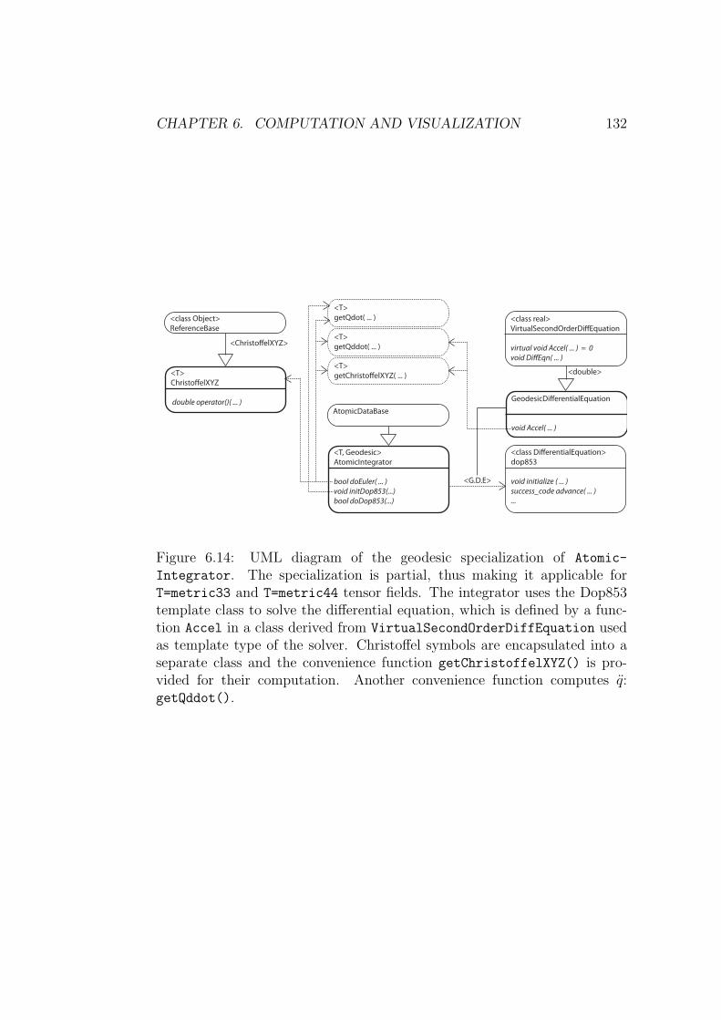
CHAPTER 6. COMPUTATION AND VISUALIZATION 132
<T, Geodesic>AtomicIntegrator
bool doEuler( ... )void initDop853(...)bool doDop853(...)
AtomicDataBase
<T>getChristoelXYZ( ... )
GeodesicDierentialEquation
void Accel( ... )
<class DierentialEquation>dop853
void initialize ( ... ) success_code advance( ... )...
<class real>VirtualSecondOrderDiEquation
virtual void Accel( ... ) = 0void DiEqn( ... )
<G.D.E>
<double><T>ChristoelXYZ
double operator()( ... )
<class Object>ReferenceBase
<ChristoelXYZ>
<T>getQdot( ... )
<T>getQddot( ... )
Figure 6.14: UML diagram of the geodesic specialization of Atomic-
Integrator. The specialization is partial, thus making it applicable forT=metric33 and T=metric44 tensor fields. The integrator uses the Dop853template class to solve the differential equation, which is defined by a func-tion Accel in a class derived from VirtualSecondOrderDiffEquation usedas template type of the solver. Christoffel symbols are encapsulated into aseparate class and the convenience function getChristoffelXYZ() is pro-vided for their computation. Another convenience function computes q:getQddot().

CHAPTER 6. COMPUTATION AND VISUALIZATION 133
component of the point is just set to zero but the time component of theinitial direction needs proper treatment.
The 4th parameter of the initial direction has to be computed dependenton the metric tensor at its position to satisfy the geodesic requirement, seeequation (2.32) in section 2.1.7.
g(q, q) = 0 (6.5)
Written in txyz coordinates and using v := q:
gµνvµvν = 0 (6.6)
After expansion:
gttvtvt +gtxv
tvx +gtyvtvy +gtzv
tvz +gxtv
xvt +gxxvxvx +gxyv
xvy +gxzvxvz +
gytvyvt +gyxv
yvx +gyyvyvy +gyzv
xvz +gztv
zvt +gzxvzvx +gzyv
zvy +gzzvzvz = 0
(6.7)
Collecting terms for vt and using the symmetry of g (gµν = gνµ) yields thequadratic equation
(vt)2 + vtB
A+C
A= 0 (6.8)
with
A = gttB = 2(gtx + gty + gtz)C = (gxxv
xvx + gyyvyvy + gzzv
zvz) + 2(gxyvxvy + gxzv
xvz + gyzvxvz).
(6.9)
Finally, leading to the two possible solutions for vt
vt1,2 = − B
2A+−
√(B
2A
)2
− C
A(6.10)
with vt1 < vt2.The implementation in the AtomicIntegrator of the geodesics always
chooses the vt2 as valid initial condition.This computation is encapsulated in the getQdot() function, see listing
6.17, line 12. It is only called for initialization. An additional feature wasadded to the function. If the initial direction is set to (0, 0, 0) then the timecoordinate will be set to 1.0 and the geodesics will represent the motion ofparticles initially being at rest instead of photons moving at the speed oflight.
Finally, the 4D geodesic module has to be registered to Vish:

CHAPTER 6. COMPUTATION AND VISUALIZATION 134
Grid
GlossyColorMapLines
linewidthpointsizeghostylinesghostypointscolorlength...
ColorMap
Range
Field
Figure 6.15: Schematic illustration of the Vish line rendering moduleGlossyColorMapLines. Primary input is the Fiber Grid connection. Ascalar field and colormap can be connected to texture the line.
1 typedef Fie ldL ine s : : I n t eg r a l L i n e s <metric44 , F i e l dL ine s : : Geodesic>2 GeodStationary4 ;3
4 stat ic Ref<VCreator<GeodStationary4 , AcceptList<Fiber : : Field>>>5 MyG44Creator ( ”Compute/ Geodes ics44 ” , ObjectQual i ty : :EXPERIMENTAL) ;
The 4D stationary geodesics are verified in section 7.3 by visualizing aSchwarzschild metric, see section 2.2, and used to explore the Kerr metric insection 7.4.
6.3 Rendering Lines
For the rendering of lines a Vish rendering module was developed. The mod-ule is based on the VBO technique and makes use of the caching mechanism,as described in section 5.2.3.
A basic module for line rendering was already included in the Vish envi-ronment. I introduced an enhanced module that allows to texture the lineswith any color-map driven by an arbitrary scalar Fiber Field stored on theline Fiber Grid.
The module primarily takes a grid object as input to get the geometrydata, the vertices and connectivity, of the lines. Thickness of the renderedlines and size of vertex points can be controlled by the parameters linewidthand pointsize. Lines and points can be transparent (normal or additive).
If no scalar field is connected to secondaryfield, 1D texture coordinatesare computed based on the length of the line needed for texturing by a color-map. If no color-map is connected a linear ramp between two user definedcolors is created, starting from green and going to red.

CHAPTER 6. COMPUTATION AND VISUALIZATION 135
GlossyColoMapLines
override <State> newState( ... )override bool update( ... )override void render(...)
VRenderObject
TimeDependent
GLTexture1DRampTexture
State
FieldState
DrawArraysMyRenderer
Figure 6.16: Uml diagram of the line rendering module. An inner state classis used that make data, extracted and computed in the update function,available in the render function. Rendering is done using a class for ren-dering data arrays (MyRenderer) utilizing VBOs, see section 5.2.3. A onedimensional color ramp is created if no color-map is providing a texture. Vishprovies a GLTexture1D class for convenience. Textures and VBOs are cachedas described in section 5.3.
To color the line by a scalar field and color-ramp, a scalar field and acolor-ramp is connected to secondaryfield and colormap. An additionalrange object can be connected as well (range) to scale and clamp the scalarfield range. A toggle between length based and scalar field coloring can beadjusted, too (colorlength). Figure 6.15 illustrates the module connectionsand parameters.
To enhance the perception of 3D curvature, highlighting or shading ofthe lines was added based on OpenGL multi texturing. The highlightingtexture is blended over the color texture additively (glBlendFunc(GL ONE,
GL ONE)). The tangential vector of the line is used as a 3D texture coordinatewhich is then transformed into a 1D coordinate by using a texture transfor-mation matrix. The matrix basically does a transformation dependent onthe view direction, thus simulating a cos(φ) between the camera axis andthe tangential line direction. The look-up in the pre-sampled 1D highlight-ing texture is added to the color of the line resulting in a shaded line. Linesbecome highlighted when the tangential vector becomes perpendicular to thecamera view axis and diffuse when oriented parallel.
Figure 6.17 illustrates six different configurations of the line renderingmodule, drawing the same line geometry.
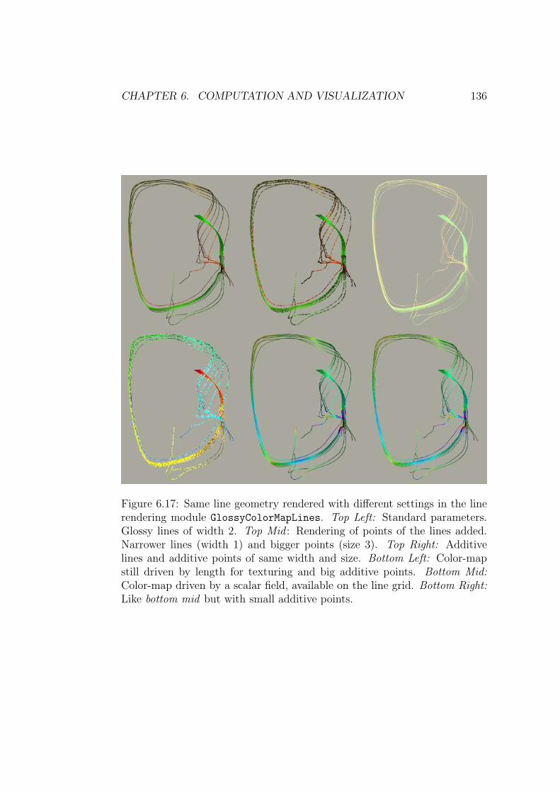
CHAPTER 6. COMPUTATION AND VISUALIZATION 136
Figure 6.17: Same line geometry rendered with different settings in the linerendering module GlossyColorMapLines. Top Left: Standard parameters.Glossy lines of width 2. Top Mid : Rendering of points of the lines added.Narrower lines (width 1) and bigger points (size 3). Top Right: Additivelines and additive points of same width and size. Bottom Left: Color-mapstill driven by length for texturing and big additive points. Bottom Mid:Color-map driven by a scalar field, available on the line grid. Bottom Right:Like bottom mid but with small additive points.

CHAPTER 6. COMPUTATION AND VISUALIZATION 137
Figure 6.16 shows the class dependencies of the rendering modules. Theupdate function extracts the line geometry and computes curvature and thelength parameter of the lines per vertex. Also, the scalar data field is ex-tracted and normalized, so that it can be used as 1D texture coordinatesfor the color map. All this data is stored in the inner state object and onlyrecomputed when the line geometry changes or other user input forces arecompute.
The render function gets all data it needs for instant rendering from thestate object. The OpenGL calls for rendering the VBOs are encapsulated ina renderer class, which in this case was extended in MyRenderer. Texturesand the VBO are cached in Vishs GLCache. Listing 6.3 shows some excerptson how this is done:
1 void GlossColorMapLines : : render ( VRenderContext&Context ) const2 3 RefPtr<Fie ldState > S = getSta t e ( Context ) ;4 i f ( ! S ) return ;5
6 /* . . . */7
8 RefPtr<ValueSet> RampValues = new ValueSet ( ) ;9 RefPtr<RampTexture> LineTexture2 ;
10
11 try12 LineTexture2 = Context (*S ) ( this ) ( RampValues ) (TEXTURE( ) ) ;13 14 catch ( const GLError&)15
16 i f ( ! LineTexture2 )17 18 r g b a f l o a t t c1 , c2 ;19 ColStart << Context >> c1 ;20 ColEnd << Context >> c2 ;21
22 LineTexture2 = new RampTexture (1 , c1 , c2 ) ;23 LineTexture2−>e n l i g h t e n ( ) ;24
25 Context [*S ] [ this ] [ RampValues ] (TEXTURE( ) ) = LineTexture2 ;26 27
28 /* . . . and s im i l a r f o r g l o s s y h i g h l i g h t t e x t u r e . . */29
30 /* . . . g e t module render parameters and s e t OpenGL s t a t e s . . . */31
32 GlossyTexture : : Render LINERENDER(* LineTexture ,33 Context . CameraSettings ) ;34

CHAPTER 6. COMPUTATION AND VISUALIZATION 138
35 /* . . . */36
37 RefPtr<ValueSet> myCacheableValues = new ValueSet ( ) ;38 string VBOKey = ”” ;39 RefPtr<VBO> myVBO;40
41 try42 43 myVBO=Context (*S−>V e r t i c e s ) ( typeid (* this ) )44 ( myCacheableValues ) (VERTEXBUFFER( ) ,VBOKey) ;45 46 catch ( . . . ) 47
48 i f ( !myVBO | | S−>reVBO)49 50 RefPtr<MemBase> Pts = S−>Vert i ce s−>c r e a t e ( ) ;51 RefPtr<VertexArray>52 VA = GL : : F i e ldBuf f e r <VertexArray > : : c r e a t e ( Pts , true ) ;53
54 myVBO=Context [*S−>V e r t i c e s ] [ typeid (* this ) ]55 [ myCacheableValues ] (VERTEXBUFFER( ) , VBOKey) ;56 myVBO−>c l e a r ( ) ;57 myVBO−>append ( VA ) ;58
59 i f ( S−>TexLength && ! ColorLen ( ) ) // use l e n g t h f o r c o l o r i n g60 61 const int TextureUnit = 1 ;62 RefPtr<TexCoordArray>63 TCA = GL : : F i e ldBuf f e r <TypedTexCoordArray<double> > : :64 c r e a t e ( TextureUnit , S−>TexLengthScaled , fa l se ) ;65
66 myVBO−>append ( TCA ) ;67 68
69 /* . . . s im i l a r f o r co lor−map and g l o s s y t e x t u r e . . . */70
71 RefPtr<MyRenderer : : EdgesArray t> EA = S−>Edges−>c r e a t e ( ) ;72
73 myVBO−>setRenderer ( new MyRenderer (74 ConvertVectorArray<unsigned int , index t > : : convert (EA) ,75 GhostL ( ) , GhostP ( ) , p o i n t s i z e , width ) ) ;76 77
78 myVBO−>c a l l ( ) ;79
First, the state object is retrieved. Then textures are prepared and storedin an GLCache associated to the Context. If the extraction of the texture fromthe cache fails, line 12, the ramp texture is created based on two color input

CHAPTER 6. COMPUTATION AND VISUALIZATION 139
attributes of the module, line 22, and stored in the cache. It is identified bythe state, the rendering module, a value set and a texture identifier, line 25.The additive texture used for highlighting (GlossyTexture), is stored in thecache similarly but using a different value set.
The texture matrix for the highlighting texture is computed by using theinner class Render of GlossTexture, providing the texture and the actualcamera settings.
Next, the a vertex buffer object containing the vertex data is tried to beextracted from the cache identified by the vertex data pointer, the renderingmodule, a value set, a vertex buffer identifier and a vertex buffer key, line 43.If this fails a new VBO has to be created, what is done in line 54. The VBOis loaded with an VertexArray in a OpenGL compatible memory layout, inline 57. The VertexArray is directly created from the Fiber Field data arrayin line 51. This is a very efficient operation because of the array layout inthe Fiber Bundle library.
Next, texture coordinate arrays are created and loaded into the VBOobject, line 59 to line 67. The connectivity of the lines is retrieved from thestate, line 71, and the custom line renderer MyRenderer is set as a rendererfor the VBO object passing the connectivity and some rendering parameters.Finally the VBO is drawn using the call function in line 78. Either it wasretrieved from the cache or created newly.
Using this caching technique most rendering calls retrieve the data out ofthe cache. Parameter changes like point size or line width do not trigger acreation of a VBO object because it is not necessary. Also, VBOs are reusedwhen a certain time step is revisited. When playing an animation in Vishonly the first run will require the creation of VBO objects. In the secondrun of the same time interval these are all retrieved from the GLCache, withall data cached in the graphics card memory.
Instead of using the texture matrix and texture blending the shading ofthe lines could also be achieved using modern shading technology. In factthere are lots of other possibilities to further enhance the rendering of linesusing OpenGL shaders.
Enhancements would include rendering transparent lines. Mapping acertain scalar data field to transparency could be a good tool to visualizecertain characteristics of data. Rendering transparent lines would involvesorting the lines when drawing, which is a non trivial problem since it has tobe done accurately enough and must be very efficient.
A nice extension would be to thicken the lines using a cylindric shape,like extruding a circle along the curve. It would be interesting to connectthe thickness to some data. Scaling and squeezing could enhance visualperception of data. When applying shape extrusion one could also blend

CHAPTER 6. COMPUTATION AND VISUALIZATION 140
between different shapes, like between a rectangular or star shape and acircle dependent on input data.
Chapter 7
Applications
This chapter demonstrates the use of the implemented Vish modules de-scribed above in different application domains.
The first application shows the computation of streamlines in an analyticvector field sampled on an uniform grid. Here, accuracy and time measure-ments verify the implemented differential equation solvers of streamlines.
The second application stems from an engineering application. It demon-strates the that the streamline algorithm was formulated independent on theunderlying discretization grid structure and shows visualization features astexturing the lines and seeding using different kinds of Fiber Grid objects.A dataset containing vector and scalar field data describing the flow of a twofluids in a stir tank are visualized.
The third application shows the computation of geodesics in the analyt-ical Schwarzschild metric sampled on a uniform grid. It is used to verifythe computation algorithms and introduces visualization techniques for thecoordinate-acceleration. The Schwarzschild metric then is explored in thexy-plane (2D).
The fourth application is an extension of the third and demonstratingcomputation geodesics in the analytic Kerr metric sampled on a uniform grid.It is explored in all three spatial dimensions and illustrates four dimensionalcoordinate-acceleration.
The fifth application utilizes spatial geodesics in a medical context. Dif-fusion tensor data is visualized stemming from a MRI scan of a brain. Itdemonstrates the high re-usability of the implemented algorithms.
Besides the illustrations showing the visualizations of the different appli-cations a schematic Vish network is shown for each application illustratingthe main modules in action, demonstrating flexibility and modularity of theVish approach.
141

CHAPTER 7. APPLICATIONS 142
7.1 Visualizing Flow of CouetteFlow
The first application is the visualization of a vector field by streamlines of aan analytically described field.
Since the integral line modules only apply to numerically provided datathe analytic vector field is sampled on a uniform grid in before. A threedimensional uniform grid is used with a resolution of 32× 32× 32.
The vector field is given by the following equation, with r2 = x2 + y2 andv = 0 if r2 < 1 or r2 > 4. The factors s and t are scaling factors. The fieldis sampled around the coordinate origin in the interval (−2.1;−2.1;−2.1) to(2.1; 2.1; 2.1).
v =
− r2−2r2 s yr2−2r2 s x
5t z
(7.1)
The vector field is a modified Couette flow. In fluid dynamics the Couetteflow describes the velocity of a viscous fluid between the gap of two opposedrotating cylinders. The vector field of the two dimensional Couette flow wasextended by a linear variation in the z-axis. This also is scaled by a parameterdependent on time.
The analytic vector field is defined in a tube like shape, with z being theaxis of the tube. The characteristics of the vector field in the z = 0 plane areillustrated on the left hand side of figure 7.1. The area where some velocityis defined can be clearly seen, with the radius r having a value between 1.0and 2.0. The vector magnitude is changing with the radius, having a highvalue at the outer radius decreasing to zero and growing again by moving tothe inner radius. The direction of the vector changes from counter clockwiseorientation to clockwise orientation referring to the z-axis.
When looking at the y = 0 slice in figure 7.1, on the right hand side, thevector dependency on the z-coordinate is illustrated. Vectors are oriented inz = 0 plane when z = 0. If z > 0 the vectors are increasingly uplifted and ifz < 0 they are pushed down, according to equation (7.1).
The following figure tries to visualize these properties of the vector fieldby using just one seeding geometry.Figure 7.2 is seeded by a point forming a uniform grid and slicing by an angleof 45 degree through the vector field volume. (Recognizing the properties ismuch easier when realtime 3D camera navigation is possible.) The figureshows the streamlines from the side and from the top. Magnitudes andorientations can be seen.
Figure 7.1 and figure 7.2 are created using the same Vish module network,which is illustrated in figure 7.3. It consists of four main parts. Modules to

CHAPTER 7. APPLICATIONS 143
Figure 7.1: Couette flow visualized using streamlines. Top Left: Seed pointson the z = 0 plane form a starry shape. The magnitude and direction of thevector field dependent of the radius can clearly be seen. Bottom Right: Seedpoint on the z = 0 plane forming a rectangular grid. The area where thevelocity is defined and the magnitude of the vectors are illustrated. Smallmagnitudes occur where streamlines get very short, see the center ring of thedisc. Right: Seed points on the y = 0 plane forming a uniform grid. Thegreater the distance to z = 0 the more the vectors become lifted up or pusheddown.

CHAPTER 7. APPLICATIONS 144
Figure 7.2: Couette flow visualized using streamlines seeded a regular gridrotated by 45 degree.
extract the vector field of the data bundle (cyan), a module to create a seedinggrid (grey), the streamline integration module (green) and the line renderingmodule (yellow). To visualize a different data set the top node that deliversthe Fiber Bundle, the CouetteFlowDataCreator, has to be exchanged.
The GeomPointDistribution may be replaced by another seeding mod-ule or even a whole subnetwork of nodes to create the seeding geometry.Figure 7.12 shows a more complex network.
Figure 7.4 illustrates the contrary orientations and uplifted and pusheddown vectors very clearly. But it does not show the definition space of thevector field. Here, four grid objects created by point distribution moduleswhere combined into one seeding grid. The circular shapes are shifted a bitalong the z-axis as that the streamlines escape the z = 0 plane.
The Couette flow vector field is a good test scenario to verify the im-plemented streamline algorithms. Especially, a test comparing accuracy andperformance of the explicit Euler and the adaptive Runge Kutta of 8th orderyielded expected results.
To compare the integration methods I seeded one streamline at the po-sition (1.0; 0.0; 0.0). Since the point is located in the z = 0 plane it shouldnot escape this plane. Also the vector field flows perfectly circular aroundthe center, the streamline should have the shape of a circle. First, I didan integration using the Dop853 and adjusted the line length, or numberof integration steps, such that the streamline forms a circle. The endpoint

CHAPTER 7. APPLICATIONS 145
Grid
GlossyColorMapLinesColorMap
Field
Grid
GeomPointDistributionBundle
CouetteFlowDataCreator
Field
Grid
StreamlineIntegrator
Grid
Bundle
Grid
GridSelector
Grid
Field
VectorFieldSelector
Range
Figure 7.3: Schematic Vish network used to create the visualizationsshown in figure 7.1 and figure 7.2. The vector field data is extractedfrom the module that creates the bundle, by first selecting a grid objectand then a vector field (cyan). The seeding geometry is created using aGeometricPointDistribution module (grey). The StreamlineIntegratordoes the computation and stores a grid of lines back into the bundle host-ing the vector field and provides a grid handle for the rendering moduleGlossyColorMapLines.
almost coincides with the start point, see top left of figure 7.5. There is nonoticeable gab between the starting line (green) and the ending line (red).
Then, I switched to Euler integration and choose a step size such thatthe same number of steps would result in a similar circle as created by theDop853 integration, see mid top of figure 7.5. Then I decreased the stepsize by half and then quarters until a visually similar circle was created.All information regarding step number step sizes and integration times aregathered in the following table1:
1Measurements were done in SVN Revision 1724 of Vish on a dell M1330 XPS latopwith 4GB RAM, Intel Core2 Duo T8300 @ 2.4Ghz and NVidia Geforce 8400M GS graphicscard. Compiled in Windows Vista 32 using gcc 3.4.2 (mingw special) in debug mode.

CHAPTER 7. APPLICATIONS 146
Figure 7.4: Couette flow visualized using streamlines seeded by four pointdistribution modules combined by three grid adder modules. The streamlinesof the inner circle flow in different circular direction compare to the outerstreamlines.

CHAPTER 7. APPLICATIONS 147
Integration Steps Stepsize Overall Time Time per Step[sec] [sec]
Dop853 1 154 - 0.406 0.0026Euler 1 154 1.5 0.031 0.0002Euler 2 92 0.75 0.015 0.0002Euler 3 164 0.1875 0.031 0.0002Euler 4 708 0.0469 0.14 0.0002Euler 5 3090 0.01172 0.639 0.0002Euler 6 12770 0.00293 2.278 0.0002
Dop853 2 474 - 1.139 0.0024Euler 7 11350 0.01172 1.997 0.0002
When comparing the speed of Euler 1 and Dop853 1 the Euler 1 out-performs the Dop853 1 by a factor of 13 but with an awful accuracy, asillustrated. When decreasing the step size of Euler to get one good circle,see bottom right of figure 7.5, now, the Dop853 1 outperforms the Euler 6by a factor of 5.6.
Another comparison was based on Euler 5 and Dop853 1. They have asimilar integration time. Based on the step size the length was now adjustedsuch that the streamline would flow around the axis for 4 times: Dop853 2and Euler 7 in the table. The streamlines illustrated in figure 7.6. The bot-tom left figure demonstrates how the Dop853 streamline still stays accuratelyon the circle, while the Euler starts to spin outwards.
Thus, the Euler integration can be fast if accuracy is not important. TheDop853 still provides good speed at high accuracy, as expected, section 6.2.1.

CHAPTER 7. APPLICATIONS 148
Figure 7.5: Comparison of the integration methods Euler and Dop853. Acorrect integration should yield a circle, like, when using Dop853 (top left).An Euler integration with the same number of steps results in a spiral shape(top mid). Decreasing the step size of the Euler integration finally yields acircle but with a higher computation time than Dop853 (top right via bottomleft to bottom right). Data according to the illustration is gather in the table.
E

CHAPTER 7. APPLICATIONS 149
Figure 7.6: Comparison of Euler 6, left, and Dop853 2, right, which have asimilar computation time. The streamline circles 4 times around the center.However, accuracy is very different. A zoom to the start point, bottomfigures, illustrate how the Euler 6 spins outwards whereas the Dop853 2stays accurately on the circle.
7.2 Visualizing Flow and Pressure in a
Stirred Fluid Tank
An application stemming from the Mechanical Engineering Department ofthe Louisiana State University is the visualization of streamlines in a stirredtank. The dataset was provided by Sumanta Acharya and Somnath Roy.
They computed the mixing of two distinct fluids in a stirred tank, which isfrequently used in chemical industries. The aim is the analysis of the mixingbehavior. If the mixing properties of the tank could be improved this wouldbe very interesting for chemical industries.
To capture the geometry of the stirred tank sophisticated methods wereused, making visualization of the results difficult or impossible with availablestandard software, such as Tecplot [56] or EnSight [37]. 2088 curvilinear multiblocks were used to discretize the computational domain by over 3 millioncells. Over 5000 time steps were produced during the simulation.
A rotating four bladed propeller induces the mixing in the cylindricaltank that has vertical baffles mounted along its walls. Figure 7.7 illustratesthe geometry of the tank.
As a result of the large eddy simulation with “Immersed Boundary Meth-

CHAPTER 7. APPLICATIONS 150
Figure 7.7: Stirred tank discretized by 2088 curvilinear blocks. The geometryof the four vertical baffles as well as the rotating axis and the curvature ofthe hemispherical bottom of the tank are modeled.
ods” the finite volume computation yielded a vector field describing the flowof the fluids and a scalar field for pressure. Data was converted to F52 formatand could then be loaded via the Fiber Bundle library into Vish.
I used the data set to apply, test and develop my integration line con-cepts for streamline seeding, computation and visualization and, especially,to make the integration independent of the underlying grid data structure,see FindLocalFromWorldPoint in section 5.4. The same algorithm can beused for uniform and curvilinear grids. Other grid types are supported byextending the FindLocalFromWorldPoint class. As soon as, for exampleAMR support is added to the local point finder, the streamline module willalso work in AMR data.
The results of the collaborative work were shown at the CCT booth onthe Supercomputing conference in 2008, Austin USA, and finally yielded acommunication paper, that I presented at WSCG 2009 [53], in Plzen CzechRepublic, see [1] also included in appendix C. This formed a basis for furtherwork mainly done by Bidur Bohara and led to a second publication (journal)at WSCG 2010, see [16], also included in appendix C.
The figures shown in this chapter illustrate different seeding strategies,compare the integration methods and demonstrate the benefit of using theFiber Bundle model as a systematic data model. In combination with themodule separation approach, utilized in the Vish network, visualization fea-tures were created that were not planned on purpose, but rather happened
2File mapping of the Fiber Bundle data model utilizing the HDF5 format, chapter 4.
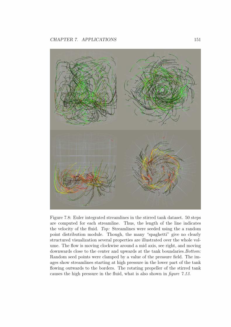
CHAPTER 7. APPLICATIONS 151
Figure 7.8: Euler integrated streamlines in the stirred tank dataset. 50 stepsare computed for each streamline. Thus, the length of the line indicatesthe velocity of the fluid. Top: Streamlines were seeded using the a randompoint distribution module. Though, the many “spaghetti” give no clearlystructured visualization several properties are illustrated over the whole vol-ume. The flow is moving clockwise around a mid axis, see right, and movingdownwards close to the center and upwards at the tank boundaries.Bottom:Random seed points were clamped by a value of the pressure field. The im-ages show streamlines starting at high pressure in the lower part of the tankflowing outwards to the borders. The rotating propeller of the stirred tankcauses the high pressure in the fluid, what is also shown in figure 7.13.

CHAPTER 7. APPLICATIONS 152
“accidentally” during implementation.Figure 7.8 gives an overall impression of the motion of the fluid by seeding
randomly in the stirred tank volume. The scalar pressure field is used toextract regions of high pressure, see section 6.1.1.
Some time measurements were done to analyze performance behaviors ofthe implemented algorithms. Figure 7.9 shows the setup that was used inthe stirred tank. Here, streamlines are seeded along a horizontal line on 12seed points close to the center of the tank.
Time was measured during the first integration process, where all Uni-GridMappers, used to speed up computation of local grid coordinates, haveto be created for each visited block, section 5.4.3. In a repeated computationpreviously computed UniGridMappers are reused, leading to a speed up inthe repeated computation of the streamline.
Figure 7.9 shows only those curvilinear multi-block outlines a Uni-GridMapper object has been created for.
Timings of Euler and Dop853 streamlines with a length of 50 and 500steps were stopped and gathered in the following table3:
Integration Steps Steps Overall Time per Speedupper Line Time [sec] Step [sec]
E50f 50 612 10.84 0.0177E50c 50 612 0.80 0.0013 13.55
E500f 500 5343 39.78 0.0074E500c 500 5343 6.506 0.0012 6.11D50f 50 612 19.02 0.0307D50c 50 612 10.70 0.0170 1.78
D500f 500 5147 131.10 0.025D500c 500 5147 93.86 0.018 1.4
Following naming convention is used for the measurements: E stands forEuler and D for Dop853. This is followed by the number of integration steps,which is followed by f, denoting a first computation or c, denoting computa-tion with all Unigridmappers of the visited blocks having been cached. Thespeed up always refers to the first and cached computation times.
When comparing the timings of the Euler integration with respect to theUniGridMapper initialization the speed up is about a factor of 10 (E50f/cand E500f/c in the table). The difference (half) of the speed up comparingthe 50 and 500 steps lines could be the consequence of the increasing distance
3Measurements were done in SVN Revision 1724 of Vish on a dell M1330 XPS latopwith 4GB RAM, Intel Core2 Duo T8300 @ 2.4Ghz and NVidia Geforce 8400M GS graphicscard. Compiled in Windows Vista 32 using gcc 3.4.2 (mingw special) in debug mode.

CHAPTER 7. APPLICATIONS 153
between integration lines. All lines start closely together. Thus, a point ofa streamline will probably be located in the same multi-block as a point ofa different streamline that was computed before. The UniGridMapper canbe reused in that case. However, with increasing integration the streamlinesmove apart and such a reuse becomes more and more unlikely, resulting in alower speedup for long integration lines.
Comparing the same timings of the Dop853 integration the speed ups aremuch smaller (D50f/c and D500f/c in the table). During the computationmany more local coordinates are computed densely on a streamline. Thus,inside a multi-block is the UniGridMapper is already reused several times.The creation process itself has a much smaller influence on the overall time.Also when computing long lines a decrease of the speed up occurs as perceivedwith the Euler integration.
When comparing Euler and Dop853 timings a similar factor of more than10 can be observed when looking at E50c/D50c and E500c/D500c. This is asimilar factor as observed in the Couetteflow table, section 7.1.
The initialization process has a much deeper impact on Euler. Thus, theDop853 requires just about double time in that case, compare E50f/D50f andE500f/D500f.
Irritating is the difference in the total number of steps in the 500 stepslines: 5343 in case of Euler and 5147 in case of Dop853. If a point of astreamline gets out of the spatial domain line computation will stop beforethe final step number is reached. This can happen in case of Euler integrationsince the step size might be too long. However, it is unlikely to happen usingthe highly accurate Dop853 solver.
This could be related to a problem of finding the local coordinates atblock boundaries. When a world point is located closely at a quite deformedboundary of a block a point can probably neither be found in one block orthe other.
Similar can occur between cells inside the multi-block. But being in-side the cell neighbors are known and used to overcome this numerical un-accuracy without using epsilons, see listing 5.22 in section 5.4.
Similar can be done when neighborhood information of the blocks is avail-able. Neighborhood information can easily be stored in the Fiber Bundlemodel as an additional Fiber Representation. Best, a file converter wouldalready copy or compute this information into the F5 format.
Further investigation should be done here, since after revisiting theLocalPointFinder during the work on pathlines with Bidur Bohara andNathan Brener (Computer Science Departments of LSU) this issue wasthought to be tackled down completely, see [16] also included in appendixC.

CHAPTER 7. APPLICATIONS 154
Figure 7.9: Streamlines seeded by a line of 10 seed points. Differentparameters were used to compare the performance gain by caching theUnigridmapper objects. Multi-blocks touched by the streamlines are shownby their outlines. Top Left: 10 Euler integrated streamlines, 50 steps. TopRight: 10 Dop853 integrated streamlines, 50 steps. Due to the short lengththey are very similar to the Euler integrated lines. Bottom Left: 10 Eu-ler integrated streamlines, 500 steps. Bottom Right: 10 Dop853 integratedstreamlines, 500 steps. The streamlines differ a lot from the Euler integratedlines. Because of the long length the difference in the integration is bigger.Still the Euler integrated lines give a very good approximation. Data ofmeasurements is collected in the table.

CHAPTER 7. APPLICATIONS 155
Figure 7.10: Streamlines seeded by a grid created by two convolution pro-cesses. A line is convolved with a smaller circle. The resulting grid is againconvoled with a bigger circle. The stirred tank is shown from top viewing innegative z-direction. Streamlines flow downwards while spinning around theaxis. The streamline ribbons remain ribbons in a quite steady circular flowuntil they reach a turbulent region where they are torn apart (region of thepropeller).

CHAPTER 7. APPLICATIONS 156
Figure 7.10 illustrates how a multiple convolution of seeding grids helps toanalyze the fluid flow. Ribbons of streamlines are created by seeding denselyalong short lines. These lines are grouped in small circles and finally copiedaround the axis of the tank to cover a bigger region.
The streamlines seeded by this geometry visualize the flow locally by theribbons as well as in wider regions. Also, the many lines do not producehardly readable “spaghetti” as seen in figure 7.8. The strong geometricalsymmetry is a result of the convolution of circles and lines. The symmetryenhances the visual result.
As described in the figure the ribbons get torn apart in the lower regionof the stirred tank. This is also illustrated in figure 7.11. Here, tube-likestreamline are seeded at a similar location as in figure 7.10. Additionally, thestreamlines are colored by the value of the magnitude of the velocity field.The labeled color-map, section 5.5, illustrates the magnitude values. Theblue to magenta colors represent a high magnitude value on the streamline.
Using the Fiber Bundle and Vish module approach any valid grid objectcan be used to seed streamlines. First, only the seed point grids describedin section 6.1.2 were used. During Werner Benger’s work on an iso-surfacemodule suitable for curvilinear grids, we realized that the iso-surface is a welldefined Fiber Grid object and, thus, valid for seeding streamlines.
One can extract features of the fluid simulation by an iso-surface, forexample, of the pressure or Laplacian field, and can seed a streamline fromthe surface. Figure 7.13 illustrates how a pressure iso-surface revealing thepropeller was used to seed the streamlines computation. More examples anddetails can be found in [1] also included in appendix C.
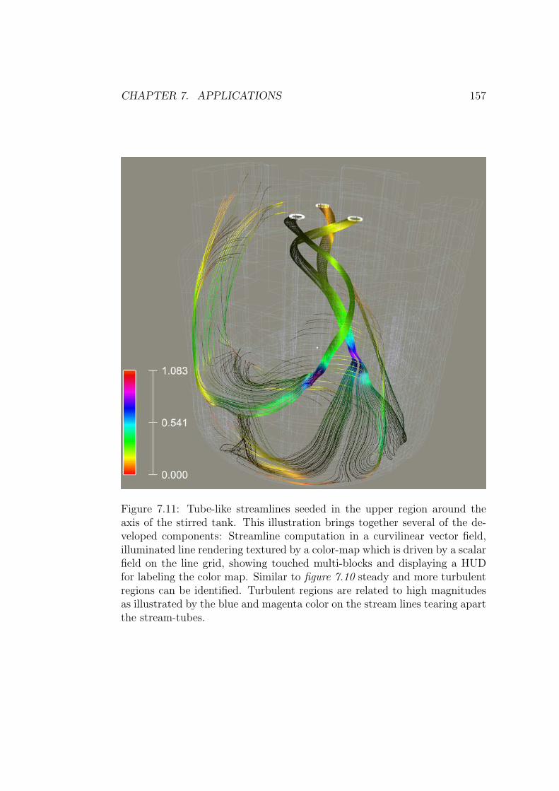
CHAPTER 7. APPLICATIONS 157
Figure 7.11: Tube-like streamlines seeded in the upper region around theaxis of the stirred tank. This illustration brings together several of the de-veloped components: Streamline computation in a curvilinear vector field,illuminated line rendering textured by a color-map which is driven by a scalarfield on the line grid, showing touched multi-blocks and displaying a HUDfor labeling the color map. Similar to figure 7.10 steady and more turbulentregions can be identified. Turbulent regions are related to high magnitudesas illustrated by the blue and magenta color on the stream lines tearing apartthe stream-tubes.
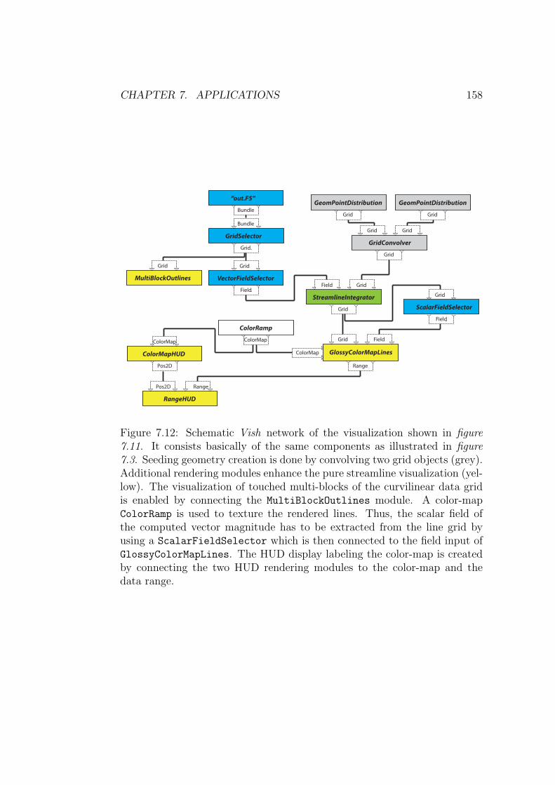
CHAPTER 7. APPLICATIONS 158
Grid
GlossyColorMapLinesColorMap
Field
Grid
Grid
GridConvolver
Grid
Grid
GeomPointDistributionBundle
“out.F5”
ColorMap
ColorRamp
Grid
GeomPointDistribution
Field
Grid
StreamlineIntegrator
Grid
Bundle
Grid
GridSelector
Grid
Field
VectorFieldSelector
Grid
Field
ScalarFieldSelector
Grid
MultiBlockOutlines
ColorMap
ColorMapHUD
RangePos2D
Pos2D
RangeHUD
Range
Figure 7.12: Schematic Vish network of the visualization shown in figure7.11. It consists basically of the same components as illustrated in figure7.3. Seeding geometry creation is done by convolving two grid objects (grey).Additional rendering modules enhance the pure streamline visualization (yel-low). The visualization of touched multi-blocks of the curvilinear data gridis enabled by connecting the MultiBlockOutlines module. A color-mapColorRamp is used to texture the rendered lines. Thus, the scalar field ofthe computed vector magnitude has to be extracted from the line grid byusing a ScalarFieldSelector which is then connected to the field input ofGlossyColorMapLines. The HUD display labeling the color-map is createdby connecting the two HUD rendering modules to the color-map and thedata range.

CHAPTER 7. APPLICATIONS 159
Figure 7.13: Streamlines seeded by an iso-surface created from a scalar pres-sure field. The iso-surface is stored as a Fiber Grid object in the Fiber Bundleand is used as the seeding grid for the streamline computation module. Thiswas not a planned feature for streamline visualization. It is, finally, thereward of using highly reusable data models and algorithms.
CHAPTER 7. APPLICATIONS 160
7.3 Visualizing Geodesics in a sampled
Schwarzschild Metric
The aim of the visualization of the Schwarzschild metric was to look at awell known simple metric and to reduce the computational complexity forthe purpose of error checking and development.
First, the metric itself had to be computed. So I implemented an an-alytic creator module that samples the Schwarzschild metric on a uniformgrid, which could be used as an numerical input data field for the geodesiccomputation module. First I tried to keep things simple and computed themetric in the xy-plane only, reducing it to 2D spatial coordinates. I thoughtI could cut off the time coordinate as well and do a purely spatial geodesiccomputation using the geodesic module in a metric33 field, section 6.2.
So I reduced the metric tensor to
g =
(
1−2mr
)−10 0
0 r2 00 0 r2sin2θ
=
(
1−2mr
)−10 0
0 r2 00 0 r2
(7.2)
with θ = π2.
This metric was transformed into Cartesian coordinates by applying equation(2.15) and stored on each point on a uniform grid object.
However, in some regions these pure spatial geodesics looked pretty well,whereas in other areas they were distracted strongly from the gravitationalcenter and some geodesics even got bent out of the xy-plane. Also, the resultchanged with different sample resolutions of the grid. While searching forthe error in the algorithm I found two errors regarding some indexing and amissing normalization of the derivatives of the metric tensor used to computethe Christoffel symbols. Since derivatives were computed in array index spacethey had to be divided by the according cell’s size.
The computed geodesics now resided on the xy-plane and did not, orjust barely, change with different grid resolutions. But the distraction stilloccurred.
I introduced a module (ComputeQddot44) that computes the coordinateacceleration vector q on any given input vector field to visually explore thedistraction of the geodesics. It takes the metric field and a 3D vector field asinput for initial directions q. It computes the Christffel symbols and q usingthe same template functions as the geodesics and outputs q as a 4D vectorfield, see figure 7.14.
I then created a new module that extracts the 3D spatial coordinates ofa 4D vector field: Vector4ToVector3AndScalar. Now, all Vish modules forrendering 3D vectors can be used to illustrate the spatial part of q.
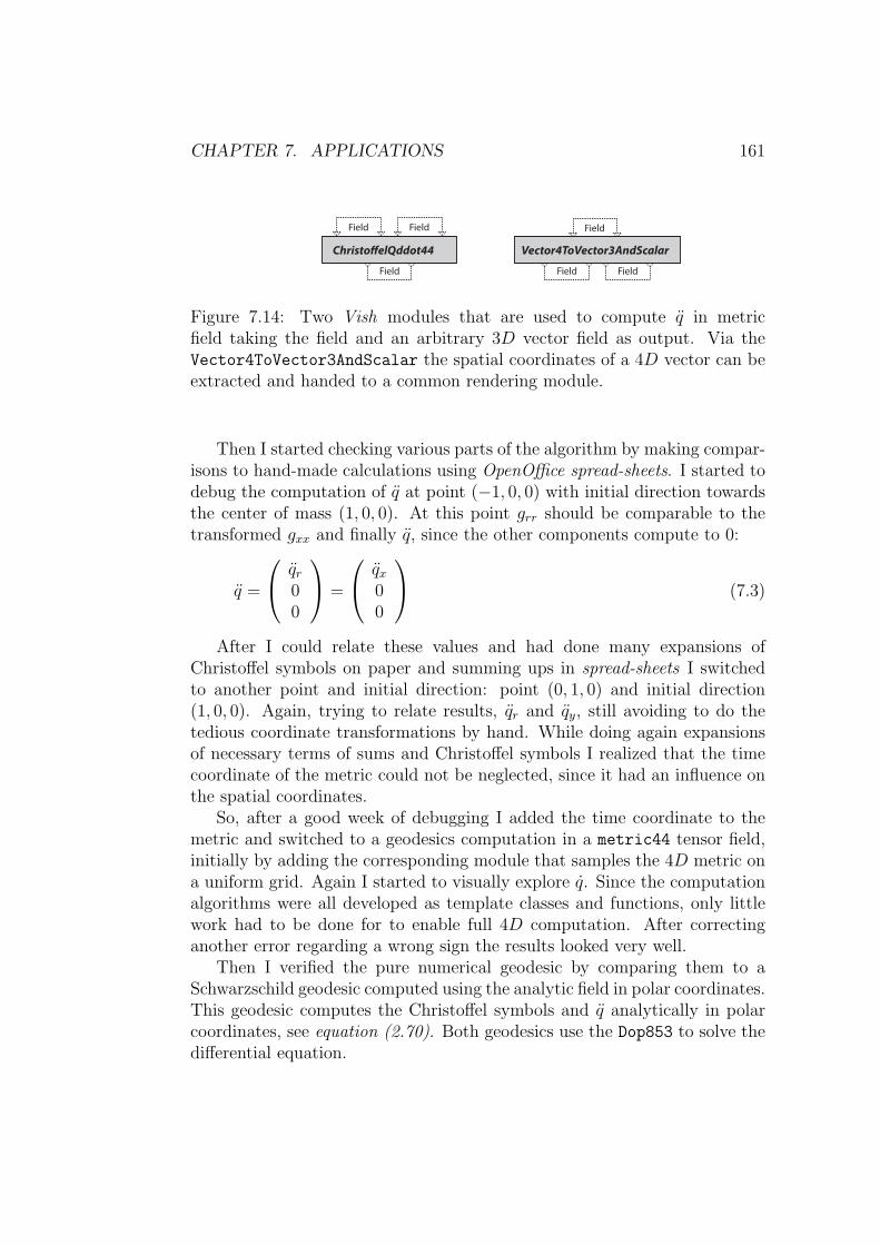
CHAPTER 7. APPLICATIONS 161
ChristoelQddot44
Field Field
Field Field Field
Vector4ToVector3AndScalar
Field
Figure 7.14: Two Vish modules that are used to compute q in metricfield taking the field and an arbitrary 3D vector field as output. Via theVector4ToVector3AndScalar the spatial coordinates of a 4D vector can beextracted and handed to a common rendering module.
Then I started checking various parts of the algorithm by making compar-isons to hand-made calculations using OpenOffice spread-sheets. I started todebug the computation of q at point (−1, 0, 0) with initial direction towardsthe center of mass (1, 0, 0). At this point grr should be comparable to thetransformed gxx and finally q, since the other components compute to 0:
q =
qr00
=
qx00
(7.3)
After I could relate these values and had done many expansions ofChristoffel symbols on paper and summing ups in spread-sheets I switchedto another point and initial direction: point (0, 1, 0) and initial direction(1, 0, 0). Again, trying to relate results, qr and qy, still avoiding to do thetedious coordinate transformations by hand. While doing again expansionsof necessary terms of sums and Christoffel symbols I realized that the timecoordinate of the metric could not be neglected, since it had an influence onthe spatial coordinates.
So, after a good week of debugging I added the time coordinate to themetric and switched to a geodesics computation in a metric44 tensor field,initially by adding the corresponding module that samples the 4D metric ona uniform grid. Again I started to visually explore q. Since the computationalgorithms were all developed as template classes and functions, only littlework had to be done for to enable full 4D computation. After correctinganother error regarding a wrong sign the results looked very well.
Then I verified the pure numerical geodesic by comparing them to aSchwarzschild geodesic computed using the analytic field in polar coordinates.This geodesic computes the Christoffel symbols and q analytically in polarcoordinates, see equation (2.70). Both geodesics use the Dop853 to solve thedifferential equation.

CHAPTER 7. APPLICATIONS 162
Figure 7.15 illustrates this verification of the numerical Cartesiangeodesics. Four different parameter settings are shown. The geodesics areseeded at point (1, 0, 0) in direction (0, 1, 0). The numerical geodesic is shownin green to red (thick line) and the analytic Schwarzschild geodesic in lightblue (thin line). Two different grid resolutions and two different values forthe mass of the black hole are shown.
With m = 0.31 (upper figures) the numerical geodesic matches the an-alytic perfectly even in the lower grid resolution. When slightly increasingthe mass to m = 0.3334 the numerical geodesic diverges from the analyticgeodesic after about a quarter of the circular motion. Increasing the gridresolution helps to converge back to the analytic solution and it matchesalmost the full circle, as shown in the lower right figure of figure 7.15.
The numerical geodesic breaks close to the event horizon of the Schwarz-schild metric, which is illustrated as a light blue thick circle. This is perfectlyexpected behavior. Here, the coordinates chosen for the numerical represen-tation of the metric have a singularity and time and space coordinates startto switch. The analytic geodesic is computed in polar coordinates, which hasno singularity at the event horizon and, thus, spirals towards the center ofgravity plunging through the event horizon.
The geodesics almost form the so-called the photon orbit of the blackhole. This orbit is found at a distance where geodesics are caught in aperfect circular trajectory around the heavy mass.
When debugging for the errors, I found looking at the q vector to be agood method to analyze the metric itself and also properties of the mappingChristoffel symbols. I used two different approaches to visualize a vectorfield of q vectors, which are illustrated in figure 7.16. The vector q vectorfield was created using two geometric point distribution modules and a gridsubtraction. The upper left figure illustrates two vector fields: q as bluearrows and q as yellow arrows. Each starting point of a vector illustratesa photon moving in the direction of the blue arrow, coordinate-acceleratedbeing in the direction of the yellow arrow. The same q field is shown in thelower left figure using vector speckles.
Vector speckles are elliptic Gaussian transparent volumes that show di-rections of vectors, as introduced in [13]. In contrast to the arrow techniquethey do not visualize the magnitude of the vector as clearly. Arrows becomevery hard to read especially when there are drawn many of them, especially in3D. Vector speckles give a better visual impression. Perception of the direc-tion is enhanced by coloring which is inspired from the physical red and blueshift. If a vector is pointing away from the observer the according speckle iscolored in red. It is colored in blue when moving towards the observer andwhite when getting parallel to the camera image plane. It also fades to white

CHAPTER 7. APPLICATIONS 163
Figure 7.15: Verification of the numerical geodesic computed in a sampledSchwarzschild metric (green and red line) by comparison to the geodesic ofthe analytic metric (thin light blue line). The thick light blue circle illustratesthe event horizon (r = 2·m) of the black hole. The brown lines show the cellsof the uniform grid. Geodesics are computed in xy-plane, indicated by theaccordingly colored lines at the border of the bounding boxes. Top: Massm = 0.31. The geodesics match perfectly, also using the coarse (16×16) grid.Bottom: Mass m = 0.3334. An increase of the grid resolution (128 × 128)leads to a better match of the numerical geodesic, which breaks at the eventhorizon because the coordinate representation of the metric has a singularityhere. The analytic geodesics is computed in polar coordinates that has nosingularity at the event horizon and, thus, spirals towards the center.

CHAPTER 7. APPLICATIONS 164
when the vector magnitude becomes small. Several parameters control thesharpness of this transition.
Thus, the color of a speckle depends on the vector direction, their magni-tude and the camera position. Coloring changes when the camera is rotated.To enable the coloring feature of the speckles the camera was slightly rotatedaround the x-axis in positive rotation direction. Otherwise all vectors wouldhave been parallel to the camera plane.
The speckles in the upper half of the lower left figure of figure 7.16 are col-ored in blue because they point towards the center and the camera. Whereas,the speckles in the lower half also point towards the center but away fromthe camera and are, thus, colored in red.
The singularity around the event horizon (black circle) is much bettervisualized than in the according image using the arrows. However, subtlechanges in the vector magnitude are better shown by the arrows.
When looking at the upper left figure the magnitude of the coordinateacceleration is greater the closer a photon is located to the mass. However, itdecreases towards the axis in direction of movement going through the centerof the black hole. Here, the magnitude decreases towards an the axis parallelto the x-axis.
The right figures of figure 7.16 illustrate the coordinate acceleration ofparticles with no initial speed. They all become attracted to the center ofgravity symmetrically. The change in the vector directions inside the eventhorizon is clearly visible also in the bottom figure by the colors of the vectorspeckles.
The next figure 7.17 illustrates the coordinate acceleration q (yellow ar-rows) dependent on different directions of velocities q (blue arrows) of pho-tons. The photons are located on a quadratic shape around the center ofgravity. They all are coordinate-accelerated towards the center with a mag-nitude dependent on the moving direction. The maximum is located to theside of the center and the minimum in the direction of the center, with ref-erence to the direction of movement.
This property holds when the velocity is rotated. The figures illustratefour rotations of the velocity. Starting in positive x direction (top left) androtating to positive y direction (bottom right).
The velocity vector is transformed to the coordinate acceleration vector bythe Christoffel symbols. The figures illustrate that a more complex structurethan, for example, a linear transformation matrix is necessary. In case of thelatter the angle between the velocity and the coordinate acceleration wouldremain constant over rotation. Here, the transformation by the Christoffelsymbols control the magnitude of the coordinate acceleration.
Figure 7.18 relates to figure 7.17. The initial directions are equal for

CHAPTER 7. APPLICATIONS 165
Figure 7.16: Schwarzschild metric is explored by the coordinate accelera-tion of moving photons (left) and the coordinate acceleration of particlesat rest(right).Top: The initial velocity is shown by blue and the coordinateacceleration by yellow arrows. The vector magnitudes are clearly visible.20×20 arrows are drawn. Bottom: Coordinate Acceleration is illustrated byvector speckles. Directions are clearly visible. The singularity at the eventhorizon is better recognized. 40 × 40 speckles are drawn. Increasing thenumber of speckles often increases the visual appearance, while the imagebecomes unreadable if the number of arrows is too high.

CHAPTER 7. APPLICATIONS 166
Figure 7.17: Illustration of the coordinate acceleration q on photons movingin different directions caused by the Schwarzschild metric. The transfor-mation by the Christoffel symbols is visualized. Velocity is illustrated asblue and coordinate acceleration as yellow arrows. Photons travel in positivex-direction (top left) and are rotated to positive y-direction (bottom rigth).

CHAPTER 7. APPLICATIONS 167
each sub-figure. Instead of the square of arrows, vector speckles are drawnin a regular grid. Initial direction become visible by the white color of thespeckles, where vector magnitude becomes small.
The two-dimensional Schwarzschild metric finally is explored by a fan ofgeodesics. Figure 7.19 shows 26 geodesics seeded at x = −1 in positive xdirection. The metric field has a resolution of 128× 128. The upper figuresshow geodesics the field with mass m = 0.01. The mass was increased tom = 0.1407 for the two lower figures. The step sizes of the integration aredirectly visualized by the yellow dots on the lines.
Comparing the upper figures, a coarse Euler and accurate Dop853 inte-gration, it turns out that the resulting geodesics are very similar. The Eulerintegration yields very good results.
I had to introduce a breaking criterion for the Euler integration, such thatgeodesics will not overshoot through the singularity. A combination of threecriteria turned out to work very well. The Euler integration stops when:
The new step size becomes greater than a constant s.
The angle of the new line segment to the old line segment exceeds aconstant angle ξ.
The computation of the norm of the new direction vector gets infinite.
When either criterion is reached the integration stops. Practical values forthe constants are: S = 4 and ξ = π/3. These values are used throughoutthe figures. These criteria could easily be made configurable by the user inthe GUI. Similar criteria could be used to improve the Euler integration bya adaptive step size control.
The Dop853 integration was not equipped with any new breaking cri-terion. It automatically refines the step size at the singularity and stopsbecause the integration gets too small some when.
Comparing the lower figures in figure 7.19 shows that geodesics far fromthe event horizon are very similar. However, if a geodesic gets close to theeven horizon the integration methods yield different results. For example, thefifth geodesic (counted from top) is orbiting halfway around the mass usingEuler (bottom left), but orbiting fully around the center using Dop853.
The geodesics are perfectly symmetrical as expected for the symmetricalmetric field. Geodesics getting too close to the center fall into the black holeand their bending decreases with distance from the center.
There is quite a difference in the computation speed of the integrationmethods here. Some time measurements of the computations shown in figure

CHAPTER 7. APPLICATIONS 168
Figure 7.18: Viusalization of q computed from different velocities. Thisfigure relates to figure 7.17. Directions of the velocity are (1, 0, 0) at top left,(1, 1, 0) at top right, (0.5, 1, 0) at bottom left and (0, 1, 0) at bottom right.These directions are shown by the speckles in white color because here themagnitude of q becomes small.
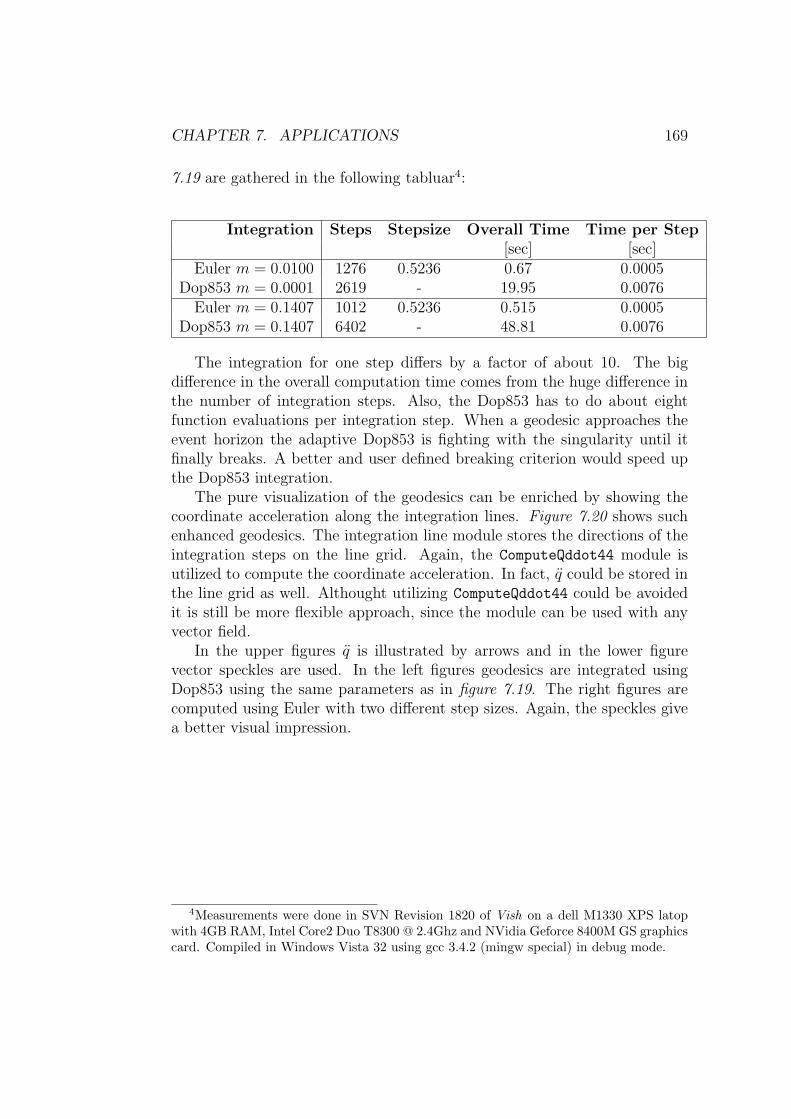
CHAPTER 7. APPLICATIONS 169
7.19 are gathered in the following tabluar4:
Integration Steps Stepsize Overall Time Time per Step[sec] [sec]
Euler m = 0.0100 1276 0.5236 0.67 0.0005Dop853 m = 0.0001 2619 - 19.95 0.0076
Euler m = 0.1407 1012 0.5236 0.515 0.0005Dop853 m = 0.1407 6402 - 48.81 0.0076
The integration for one step differs by a factor of about 10. The bigdifference in the overall computation time comes from the huge difference inthe number of integration steps. Also, the Dop853 has to do about eightfunction evaluations per integration step. When a geodesic approaches theevent horizon the adaptive Dop853 is fighting with the singularity until itfinally breaks. A better and user defined breaking criterion would speed upthe Dop853 integration.
The pure visualization of the geodesics can be enriched by showing thecoordinate acceleration along the integration lines. Figure 7.20 shows suchenhanced geodesics. The integration line module stores the directions of theintegration steps on the line grid. Again, the ComputeQddot44 module isutilized to compute the coordinate acceleration. In fact, q could be stored inthe line grid as well. Althought utilizing ComputeQddot44 could be avoidedit is still be more flexible approach, since the module can be used with anyvector field.
In the upper figures q is illustrated by arrows and in the lower figurevector speckles are used. In the left figures geodesics are integrated usingDop853 using the same parameters as in figure 7.19. The right figures arecomputed using Euler with two different step sizes. Again, the speckles givea better visual impression.
4Measurements were done in SVN Revision 1820 of Vish on a dell M1330 XPS latopwith 4GB RAM, Intel Core2 Duo T8300 @ 2.4Ghz and NVidia Geforce 8400M GS graphicscard. Compiled in Windows Vista 32 using gcc 3.4.2 (mingw special) in debug mode.

CHAPTER 7. APPLICATIONS 170
Figure 7.19: A fan of 26 geodesics is seeded at x = −1 in positive x direction.The left figures are computed using Euler and a step size of 0.5326 and theright figures are computed using Dop853. The mass for the upper figures hasa value of m = 0.01 and in the lower figures m = 0.2. Geodesic are symmetricin y direction. Euler and Dop863 integration match very well with small massand big distance from the center. When getting close results differ, comparelower images: the fifth geodesic counting from top.

CHAPTER 7. APPLICATIONS 171
Figure 7.20: Geodesics enhanced by showing the coordinate accelerationalong the lines. Left: Dop853 integration. Right: Euler integration withdifferent step sizes. Arrows are used in the upper figures, which become hardto read when too many arrows are drawn, see center of left upper figure. Vec-tor speckles illustrate the coordinate acceleration in the lower figures. Theyremain readable even when many speckles are drawn.

CHAPTER 7. APPLICATIONS 172
The next step was to move to the full 4D Schwarzschild metric withvariable θ, see eq(). I extended the metric sampling module and started toanalyze the space-time first by looking at q. Figure 7.21 shows different pa-rameters for the mass using, again, the speckle technique. Also q is pointingin positive x-direction. The singularity at the event horizon is illustratedclearly by the three axis aligned speckle planes.
Then I verified the spherical symmetry of the metric by seeding geodesicson a circular shape in the yz-plane. Figure 7.22 illustrates the geodesics thatget bent symmetrically around the black hole. Mass was increased startingfrom m = 0.1 to m = 0.3. The symmetry is best shown in the left lowerfigure where all geodesics intersect in one point after having orbited aroundthe center of mass.
Another figure illustrating was created by seeding geodesics on a verticaland horizontal line in the yz-plane. Figure 7.23 shows the result. I noticedsome geodesics that are reflected at the event horizon, see left figure. Sixgeodesics starting close to the center of the seeding cross get reflected. In-creasing the sampling of the metric field from 64× 64× 64 to 128× 128× 64yielded a better result, see right figure. Thus, I used the increased samplingfor the following analysis.

CHAPTER 7. APPLICATIONS 173
Figure 7.21: Vector speckles illustrating q sampled on three axis alignedplanes of a 3D Schwarzschild based on a q going in positive x direction. Thecoordinate acceleration is pointing to the center showed by the direction andcolor of the speckles. The spherical singularity at the event horizon(blackcircles) is clearly illustrated. Also, the small magnitude of the vectors at thex-aligned axis going through the center of the black hole is indicated by thewhite color.
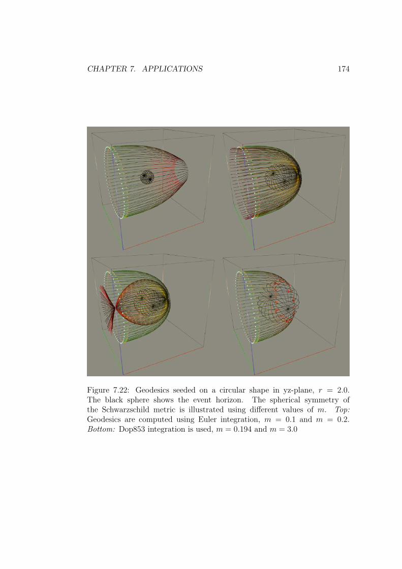
CHAPTER 7. APPLICATIONS 174
Figure 7.22: Geodesics seeded on a circular shape in yz-plane, r = 2.0.The black sphere shows the event horizon. The spherical symmetry ofthe Schwarzschild metric is illustrated using different values of m. Top:Geodesics are computed using Euler integration, m = 0.1 and m = 0.2.Bottom: Dop853 integration is used, m = 0.194 and m = 3.0
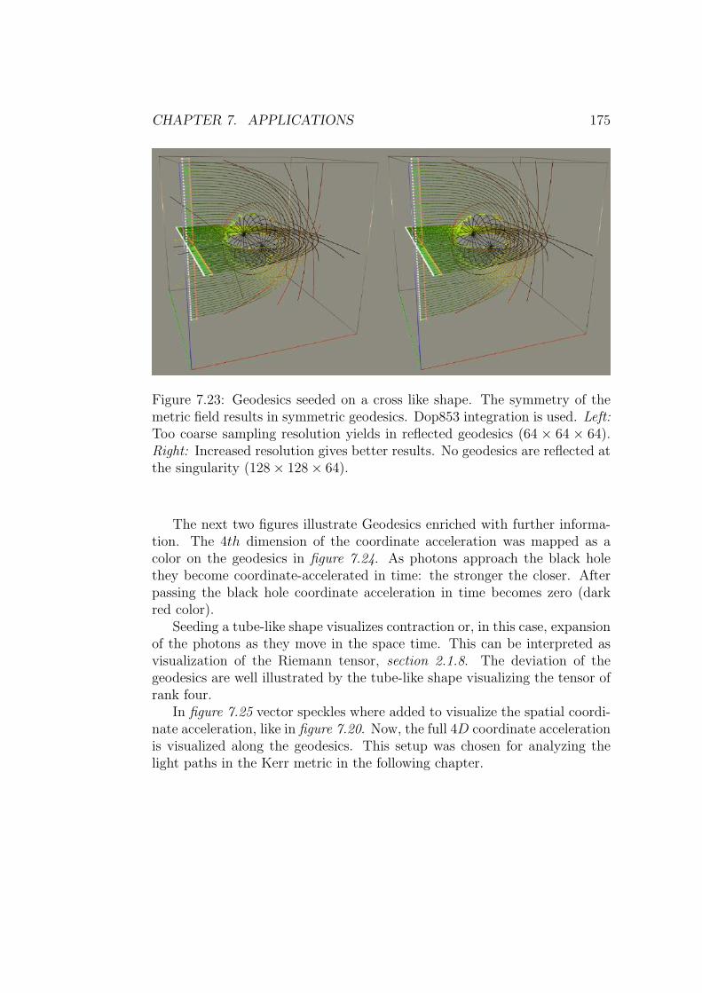
CHAPTER 7. APPLICATIONS 175
Figure 7.23: Geodesics seeded on a cross like shape. The symmetry of themetric field results in symmetric geodesics. Dop853 integration is used. Left:Too coarse sampling resolution yields in reflected geodesics (64 × 64 × 64).Right: Increased resolution gives better results. No geodesics are reflected atthe singularity (128× 128× 64).
The next two figures illustrate Geodesics enriched with further informa-tion. The 4th dimension of the coordinate acceleration was mapped as acolor on the geodesics in figure 7.24. As photons approach the black holethey become coordinate-accelerated in time: the stronger the closer. Afterpassing the black hole coordinate acceleration in time becomes zero (darkred color).
Seeding a tube-like shape visualizes contraction or, in this case, expansionof the photons as they move in the space time. This can be interpreted asvisualization of the Riemann tensor, section 2.1.8. The deviation of thegeodesics are well illustrated by the tube-like shape visualizing the tensor ofrank four.
In figure 7.25 vector speckles where added to visualize the spatial coordi-nate acceleration, like in figure 7.20. Now, the full 4D coordinate accelerationis visualized along the geodesics. This setup was chosen for analyzing thelight paths in the Kerr metric in the following chapter.

CHAPTER 7. APPLICATIONS 176
Figure 7.24: Geodesics forming a tube-like shape. Expansion is illustrated.The color on the lines represent the time component of q. It becomes zeroafter passing the black hole. To visualize the geometry of the 3D lines threeaxis aligned camera setups and one free camera position were chosen. Thetube-like shape reveals the deviation of the geodesics and thus visualizes theRiemann tensor, which is a tensor of rank four.

CHAPTER 7. APPLICATIONS 177
Figure 7.25: Like figure 7.24. Vector speckles were added to illustrate thespatial components of q.
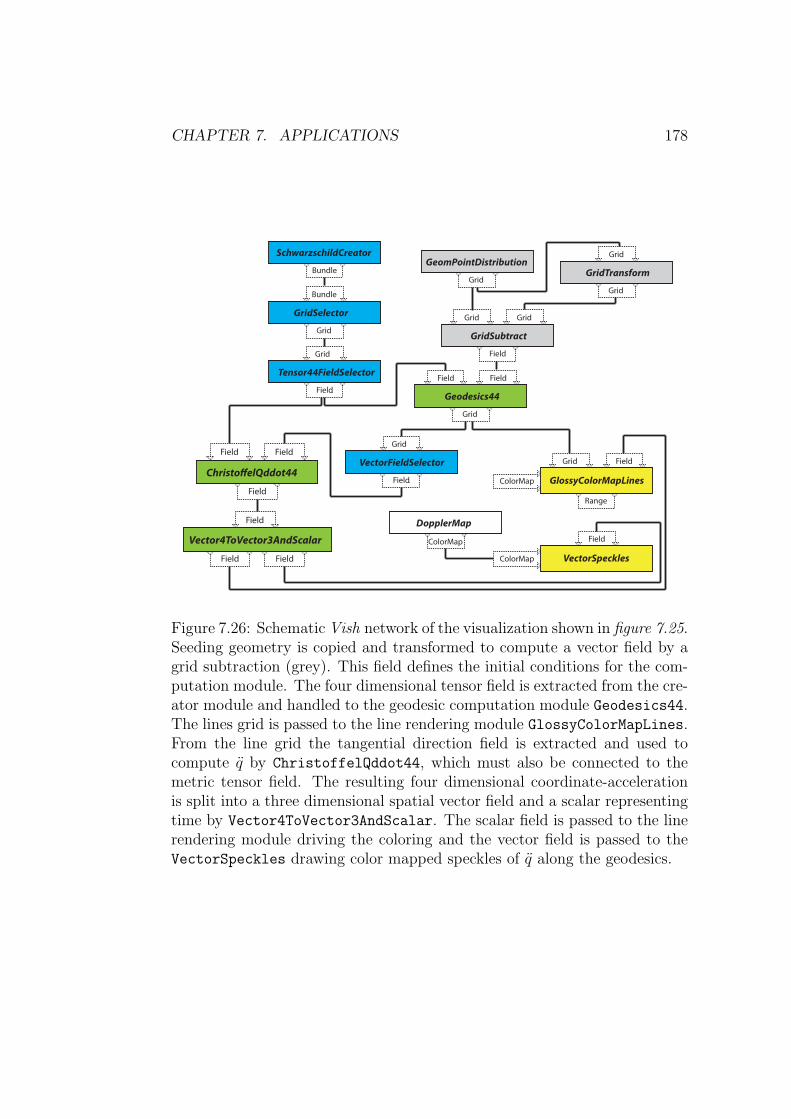
CHAPTER 7. APPLICATIONS 178
Grid
GlossyColorMapLinesColorMap
Field
Grid
Grid
GridTransformGrid
GeomPointDistributionBundle
SchwarzschildCreator
Field
Grid
Geodesics44
Field
Bundle
Grid
GridSelector
Grid
Field
Tensor44FieldSelector
Grid
Field
VectorFieldSelector
Range
Grid
Field
GridSubtract
Grid
ColorMap
DopplerMap
ChristoelQddot44
Field Field
Field
Field Field
Vector4ToVector3AndScalar
Field
VectorSpecklesColorMap
Field
Figure 7.26: Schematic Vish network of the visualization shown in figure 7.25.Seeding geometry is copied and transformed to compute a vector field by agrid subtraction (grey). This field defines the initial conditions for the com-putation module. The four dimensional tensor field is extracted from the cre-ator module and handled to the geodesic computation module Geodesics44.The lines grid is passed to the line rendering module GlossyColorMapLines.From the line grid the tangential direction field is extracted and used tocompute q by ChristoffelQddot44, which must also be connected to themetric tensor field. The resulting four dimensional coordinate-accelerationis split into a three dimensional spatial vector field and a scalar representingtime by Vector4ToVector3AndScalar. The scalar field is passed to the linerendering module driving the coloring and the vector field is passed to theVectorSpeckles drawing color mapped speckles of q along the geodesics.

CHAPTER 7. APPLICATIONS 179
7.4 Visualizing Geodesics in a sampled Kerr
Metric
After verifying the geodesic computation and exploring the symmetricalSchwarzschild field, a more complex spacetime is analyzed using the pre-viously described techniques. This chapter focuses on the visualization ofthe Kerr metric, section 2.2.3. Thus, emphasis is on the figures. Textualexplanations are kept short. “A picture is worth a thousand words”. Theprevious chapter should have been read to be able the read and interpret thefigures correctly.
Again, the a Vish module was created to sample the metric field on auniform grid. Therefore, equation (2.74) and equation (2.15) were utilized.An additional parameter now controls the angular momentum of the blackhole around the z-axis. The Kerr metric is still a stationary field withoutevolution over time. Thus, the geodesics computed here are an analogue tostreamlines in CFD.
To explore the Kerr metric I use series of figures with varying angular mo-mentums. Often more than one camera perspective is necessary to illustratethe 3D geometry unambiguously.
First some figures show the coordinate-acceleration vector by given initialspeed, again, always along the positive x-direction. I tried several seedinggeometries. First, the 3D cross similar to figure 7.21, see figure 7.27. Theangular momentum is increased by constant mass. Comparing the xy-planesof the two upper figures shows that the coordinate acceleration is starting tospin clockwise around the center of gravity. What is shown clearly is thatthe field loses its spherical symmetry around the center.
Next, geodesics were seeded in the xy-plane of the metric in x-direction.Again, starting the exploration in a reduced two/dimensional case. Figure7.28 and figure 7.29 show a series of eight figures with increasing angularmomentum. The angular momentum is from left to right and from top tobottom:
a = 0.0,a = 0.01,a = 0.05,a = m = 0.15;a = 0.25,a = 0.5,a = 0.75,a = 1.0.
The illustrations with a > m maybe have no physical meaning. Here, the
CHAPTER 7. APPLICATIONS 180
event horizon at r+ becomes undefined, section 2.2.3. However, the param-eter analysis was also done with some out-of-range values since they showcharacteristics in an over-exaggerated way.
The white or black sphere in the following figures represents the eventhorizon of a Schwarzschild black hole with the corresponding mass. Whenlooking at the locations where the geodesics break, it is observed that theevent horizon r+ of the Kerr black hole shrinks as the angular momentumincreases.
The first figure in figure 7.28 illustrates how the geodesics on the upperhalf are bent toward the center and collide earlier with the black hole, whilethe geodesics on the lower half are bent away from the black hole. The sin-gularity moves inwards with increasing angular momentum. Geodesics thatare bent away from the black hole coordinate-accelerate in time componentagain after having passed the black hole.
When increasing the angular momentum over the value of mass, geodesicson the lower half are straightened out by the rotation, see right top figure offigure 7.29 (a = 0.5) and finally become reflected.

CHAPTER 7. APPLICATIONS 181
Figure 7.27: Vector speckles on axis aligned planes in a Kerr metric illustrat-ing q with q = (1, 0, 0). The angular momentum a is increased, but holdingthe mass m = 0.2. From left to right and top to bottom: a = 0.0, a = 0.1,a = m = 0.2, a = 1.0. The Kerr event horizon at r+ shrinks when the angu-lar momentum is increased. The corresponding Schwarzschild event horizonis illustrated by the circles (black). The coordinate acceleration is spinningaround the center, what is illustrated on the xy-plane.

CHAPTER 7. APPLICATIONS 182
Figure 7.28: Geodesics seeded in the xy-plane on the line x = −1.0 in positivex-direction. With constant mass m = 0.15 the clockwise angular momentuma is increased. Geodesics in the upper half get more attracted to the blackhole, whereas the geodesics in the lower half are less attracted. The r+ eventhorizon shrinks with increasing angular momentum. When geodesics passthe black hole they are not further coordinate-accelerated in time.

CHAPTER 7. APPLICATIONS 183
Figure 7.29: Continuation of figure 7.28. Here a > m and hence the illustra-tions have no physical meaning.
CHAPTER 7. APPLICATIONS 184
Before seeding geodesics in the 3D volume I tried to look at the co-ordinate acceleration of the whole volume. First I tried to do some cu-bic slices as shown in figure 7.30. Seeding was done by using threeGeometricPointDistribution modules for the cubics together with twoGridAdder operations and one GridTransform with one GridSubtractor
to create the q vector field.The field is symmetric in the beginning (top left). Here, also the spher-
ical singularity is observable. When increasing the angular momentum onecan see that the directions are influenced by the momentum. With smallmomentum the influence applies at the nearer regions. As it grows also re-gions further away from the center are changing directions. The sphericalsingularity vanishes as it shrinks into the smallest cube.
The vector-speckle module allows to animate the speckles in a repeatedcycle motion to indicate the direction. The animated speckles give a verygood visual impression of q.
I tried a different seeding strategy over the whole volume. TheRandPointDistribution was used to create randomly distributed speck-les. Figure 7.31 again shows different values for the angular momentum,which is zero in the top left figure. Surprisingly, the randomly distributedspeckles give a quite good illustration over the volume and certain regionsof the coordinate-acceleration flow become visible. Interactive camera rota-tion helps a lot for exploration. Illustrating axis-aligned views reveals someproperties of the randomly speckled flow field.
Figure 7.32 illustrates some properties of the coordinate acceleration flowfield based on a movement in positive z-direction. The flow field is symmet-rical to one plane in the upper and lower images. It is even symmetric totwo planes in the mid figures. The left figures show an angular momentumof a = 0.2 and the right figures a = 1.0. Mass is set to m = 0.2 for all figures.
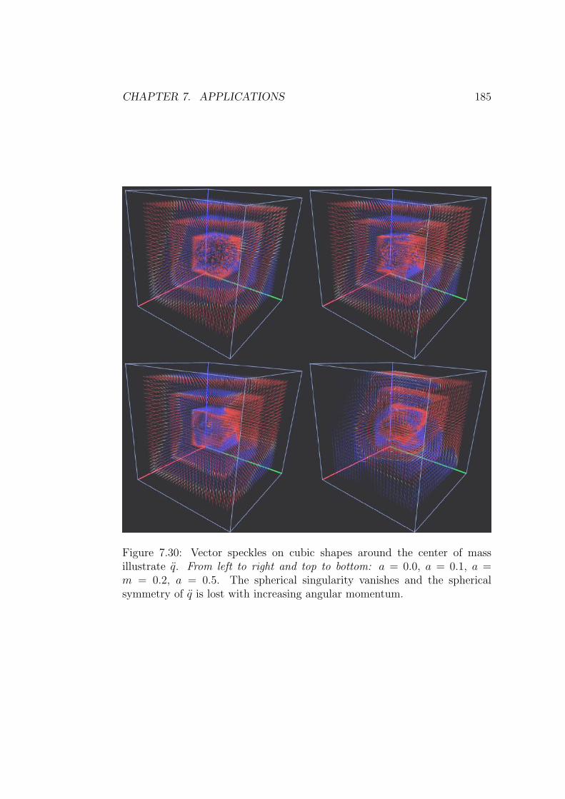
CHAPTER 7. APPLICATIONS 185
Figure 7.30: Vector speckles on cubic shapes around the center of massillustrate q. From left to right and top to bottom: a = 0.0, a = 0.1, a =m = 0.2, a = 0.5. The spherical singularity vanishes and the sphericalsymmetry of q is lost with increasing angular momentum.

CHAPTER 7. APPLICATIONS 186
Figure 7.31: Randomly distributed vector speckles illustrate q over the wholegrid volume. From left to right and top to bottom: a = 0.0, a = 0.1,a = m = 0.2, a = 0.5. This method gives a good impression over the wholevolume showing vortices and flow concentrations, not visible in figure 7.30.Especially when enabling the repeated animation of the speckles the flow isvisualized very well. On paper this is not possible. But some axis-alignedillustration of the same kind reveal some properties as well, see figure 7.32.
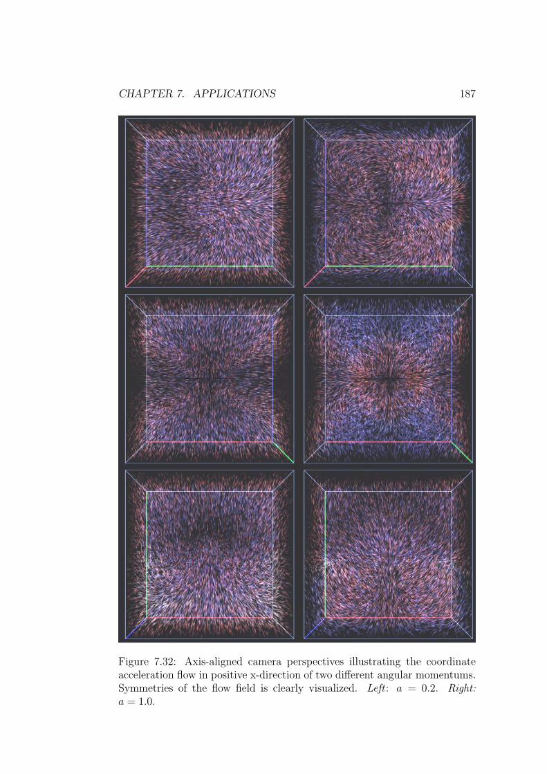
CHAPTER 7. APPLICATIONS 187
Figure 7.32: Axis-aligned camera perspectives illustrating the coordinateacceleration flow in positive x-direction of two different angular momentums.Symmetries of the flow field is clearly visualized. Left : a = 0.2. Right:a = 1.0.

CHAPTER 7. APPLICATIONS 188
Next, geodesics on a centered vertical line are illustrated in figure 7.33 andfigure 7.34, once again showing a series with increasing angular momentum.The upper left figure is similar to figure 7.23. By increasing the momentumthe geodesics below and above the event horizon are bent in direction of thepositive y axis and are less attracted to the center of gravity. The geodesicsare symmetrical to the xy-plane.

CHAPTER 7. APPLICATIONS 189
Figure 7.33: Geodesics seeded in positive x direction with m = 0.2 anda = 0.0, a = 0.01, a = 0.1 and a = 0.15. With introducing the angularmomentum the geodesics above and below the event horizon are bent inpositive y-direction.
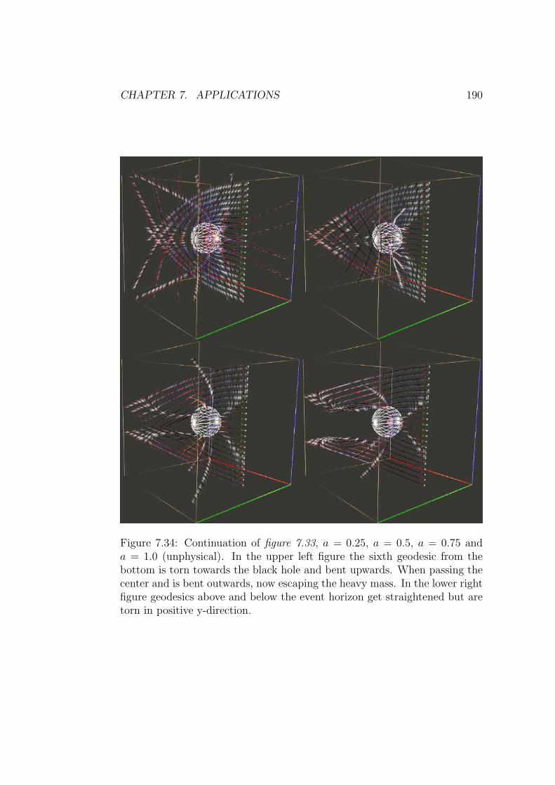
CHAPTER 7. APPLICATIONS 190
Figure 7.34: Continuation of figure 7.33, a = 0.25, a = 0.5, a = 0.75 anda = 1.0 (unphysical). In the upper left figure the sixth geodesic from thebottom is torn towards the black hole and bent upwards. When passing thecenter and is bent outwards, now escaping the heavy mass. In the lower rightfigure geodesics above and below the event horizon get straightened but aretorn in positive y-direction.

CHAPTER 7. APPLICATIONS 191
A similar setup as in the left lower figure of figure 7.22 is used to furtherexplore the metric. Again, geodesics are seeded on a circle in the yz-plane,such that they all intersect in one point, if no angular momentum is presentand the angular moment is increased. The following five figures show theseries from three different axis aligned camera perspectives.
When looking at the spacetime from top, see figure 7.35 and upper fig-ures of figure 7.36, a similar behavior to the 2D analysis can be observed.Geodesics with a greater distance to the xy-plane through the center of grav-ity are less influenced by the angular momentum. Reflections only occurclose to that plane with very strong momentum. Geodesics are symmetricto the xy-plane, which is illustrated in the lower figures of figure 7.36 and infigure 7.37, figure 7.38 and figure 7.39.

CHAPTER 7. APPLICATIONS 192
Figure 7.35: Geodesics seeded in positive x-direction on a circle in the yz-plane: m = 0.2, a = 0.0 (top left), a = 0.01 (top right), a = 0.05 (bottomleft), a = 0.2 (bottom right). View in negative z-direction. With a = 0geodesics are almost located on the photon orbit of the Schwarzschild blackhole. A slight increase in the angular momentum breaks the symmetry (topright). Geodesics seeded in the upper part of the figure are curved strongertowards the event horizon. Some of them already fall through it. In contrast,the geodesics on the lower part are less attracted towards the center. Furtherincrease of the momentum intensifies this effect. Again, the shrinking ofthe coordinate singularity can be seen, as geodesics break inside the formerSchwarzschild radius (white). Bottom right: The geodesic in the mid of thefigure is first bent in y-direction and then, when getting closer to the xy-planestrongly coordinate-accelerated toward the center in negative y-direction.
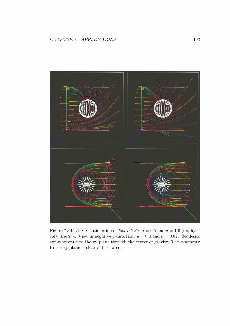
CHAPTER 7. APPLICATIONS 193
Figure 7.36: Top: Continuation of figure 7.35: a = 0.5 and a = 1.0 (unphysi-cal). Bottom: View in negative y-direction: a = 0.0 and a = 0.01. Geodesicsare symmetric to the xy-plane through the center of gravity. The symmetryto the xy-plane is clearly illustrated.
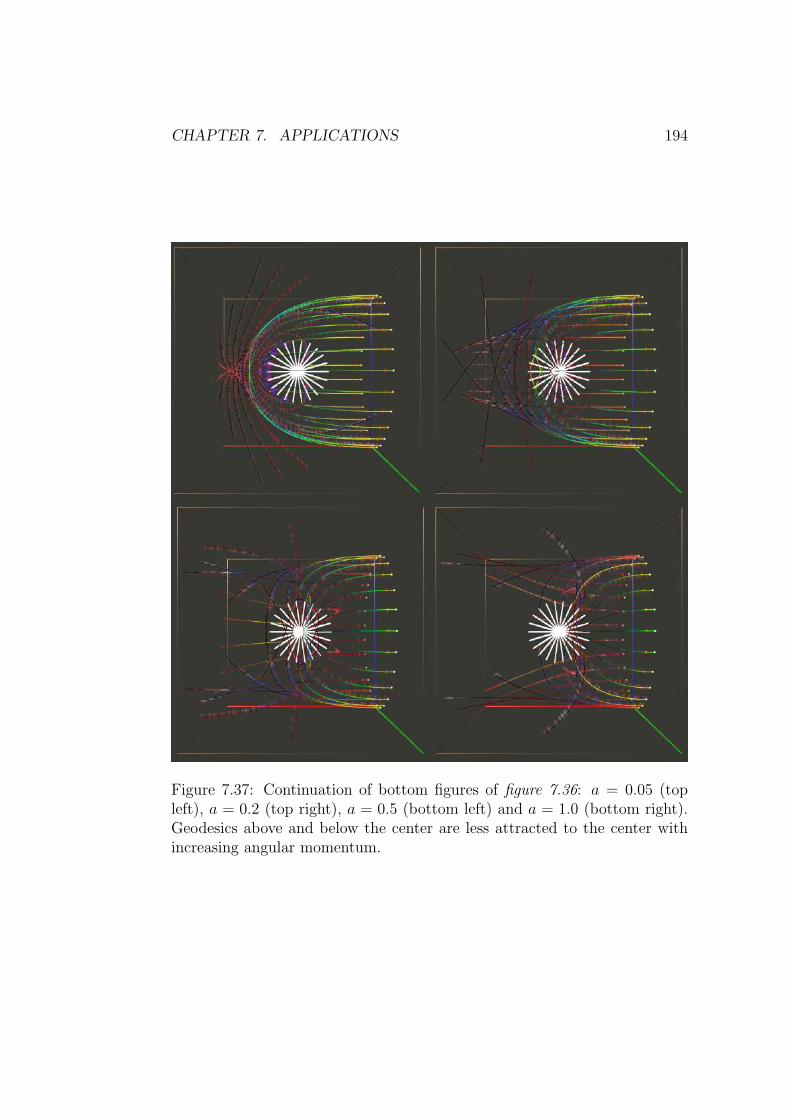
CHAPTER 7. APPLICATIONS 194
Figure 7.37: Continuation of bottom figures of figure 7.36: a = 0.05 (topleft), a = 0.2 (top right), a = 0.5 (bottom left) and a = 1.0 (bottom right).Geodesics above and below the center are less attracted to the center withincreasing angular momentum.

CHAPTER 7. APPLICATIONS 195
Figure 7.38: View in negative x-direction: a = 0.0 (top left), a = 0.01(top right), a = 0.05 (bottom left), a = 0.2 (bottom right). Geodesics aresymmetric to the xy-plane through the center of gravity.
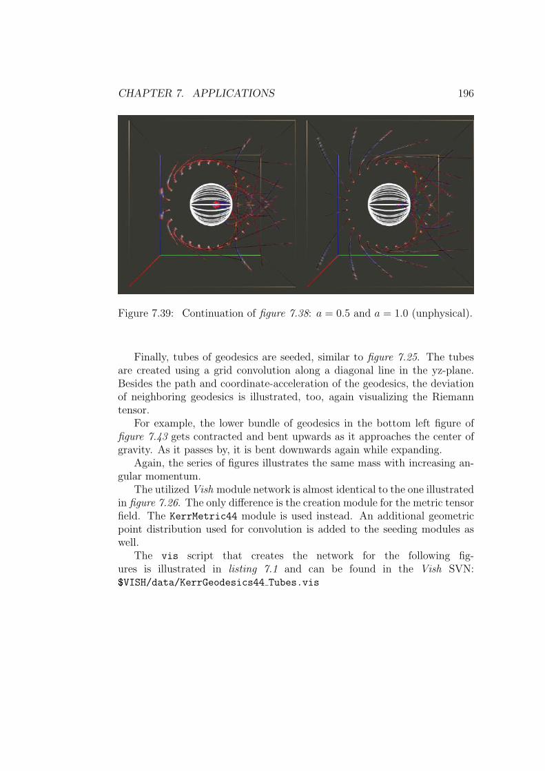
CHAPTER 7. APPLICATIONS 196
Figure 7.39: Continuation of figure 7.38: a = 0.5 and a = 1.0 (unphysical).
Finally, tubes of geodesics are seeded, similar to figure 7.25. The tubesare created using a grid convolution along a diagonal line in the yz-plane.Besides the path and coordinate-acceleration of the geodesics, the deviationof neighboring geodesics is illustrated, too, again visualizing the Riemanntensor.
For example, the lower bundle of geodesics in the bottom left figure offigure 7.43 gets contracted and bent upwards as it approaches the center ofgravity. As it passes by, it is bent downwards again while expanding.
Again, the series of figures illustrates the same mass with increasing an-gular momentum.
The utilized Vish module network is almost identical to the one illustratedin figure 7.26. The only difference is the creation module for the metric tensorfield. The KerrMetric44 module is used instead. An additional geometricpoint distribution used for convolution is added to the seeding modules aswell.
The vis script that creates the network for the following fig-ures is illustrated in listing 7.1 and can be found in the Vish SVN:$VISH/data/KerrGeodesics44 Tubes.vis
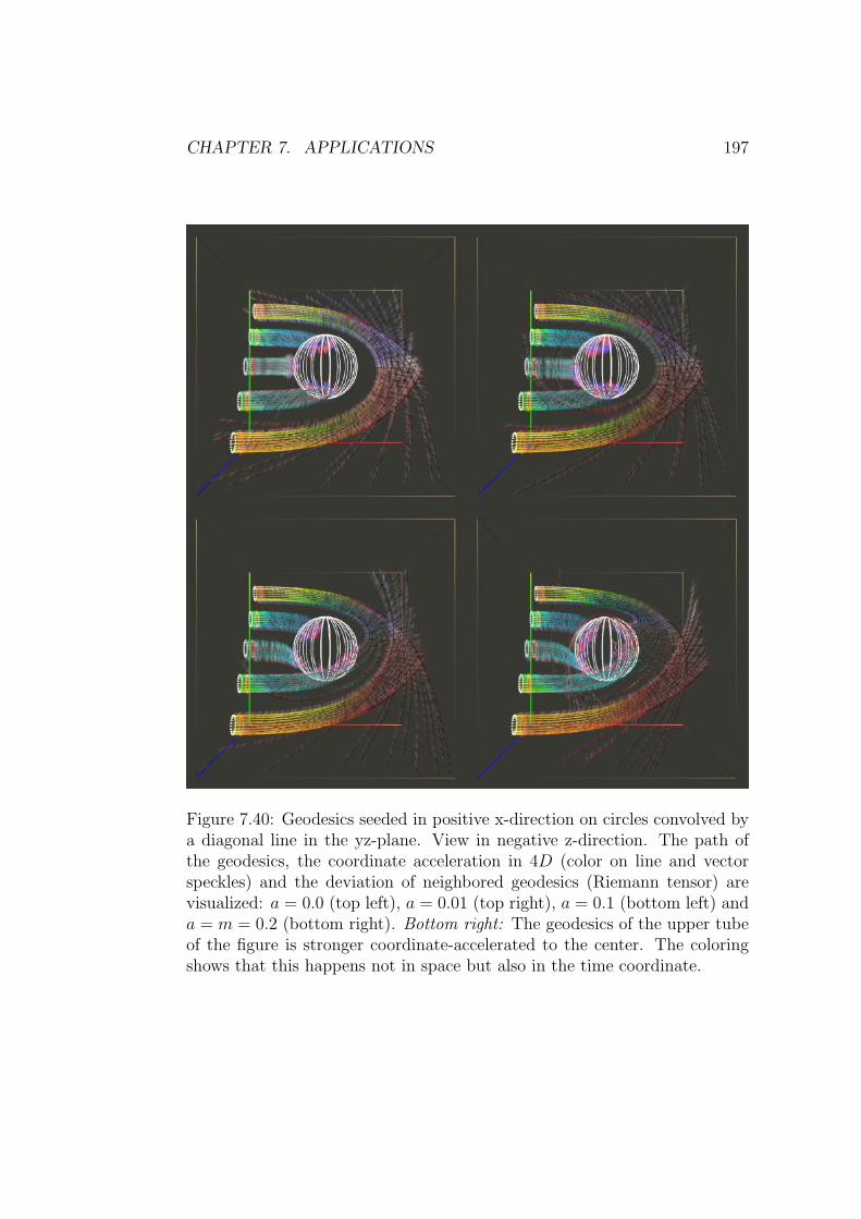
CHAPTER 7. APPLICATIONS 197
Figure 7.40: Geodesics seeded in positive x-direction on circles convolved bya diagonal line in the yz-plane. View in negative z-direction. The path ofthe geodesics, the coordinate acceleration in 4D (color on line and vectorspeckles) and the deviation of neighbored geodesics (Riemann tensor) arevisualized: a = 0.0 (top left), a = 0.01 (top right), a = 0.1 (bottom left) anda = m = 0.2 (bottom right). Bottom right: The geodesics of the upper tubeof the figure is stronger coordinate-accelerated to the center. The coloringshows that this happens not in space but also in the time coordinate.

CHAPTER 7. APPLICATIONS 198
Figure 7.41: Over exaggerated and unphysical continuation of figure 7.40:a = 0.25 (top left), a = 0.5 (top right), a = 0.75 (bottom left) and a = 1.0(bottom right).

CHAPTER 7. APPLICATIONS 199
Figure 7.42: Like figure 7.40 but view in negative y-direction: a = 0.0 (topleft), a = 0.01 (top right), a = 0.1 (bottom left) and a = m = 0.2 (bottomright). The tubes close to the center axis are contracted, whereas the outertubes are expanding. Time acceleration is increasing towards the center.Symmetry is lost with increase of the angular momentum.

CHAPTER 7. APPLICATIONS 200
Figure 7.43: Unphysical continuation of figure 7.42: a = 0.25 (top left),a = 0.5 (top right), a = 0.75 (bottom left) and a = 1.0 (bottom right).

CHAPTER 7. APPLICATIONS 201
Listing 7.1: The vis script defines the Vish module network forthe illustrations in figure 7.40. The script is located in the SVN:$VISH/data/KerrGeodesics44 Tubes.vis
1 CreateBundle / KerrMetric44 b lackho l e2 b lackho l e . t imes teps=103 b lackho l e .m=0.24 b lackho l e . a=0.25 b lackho l e . gr ids izeXY=1286 b lackho l e . g r i d s i z e Z =647
8 Fiber /Grid bh gr id9 bh gr id . spacet ime=>b lackho l e
10 <bh gr id>11
12 Fiber / Tensor f i e ld4D b h f i e l d13 b h f i e l d . g r id=>bh gr id14 <b h f i e l d >15
16 U t i l i t y /Point3D Point17 Point . range Viewer1=118 Point . xViewer1 =0.019 Point . yViewer1 =0.020 Point . zViewer1 =0.021 <PointViewer1>22
23 U t i l i t y /Point3D Point224 Point2 . range Viewer1=125 Point2 . xViewer1=−1.026 Point2 . yViewer1 =0.027 Point2 . zViewer1 =0.028 <PointViewer1>29
30 U t i l i t y /Point3D PointDir31 PointDir . range Viewer1=132 PointDir . xViewer1=133 PointDir . y=>Point . y34 PointDir . z=>Point . z35 <PointDir Viewer1>36
37 Converters / FloatsToRotor Rotate38 Rotate . yang=9039
40 Converters / FloatsToRotor Rotate241 Rotate2 . zang=9042
43 CreateFiber / Po in tD i s t r i bu t i on GridPoints44 GridPoints . p o s i t i o n=>Point45 GridPoints . r o t a t i o n=>Rotate

CHAPTER 7. APPLICATIONS 202
46 GridPoints . l ength =0.247 GridPoints . l eng th subd iv s =1048 GridPoints . he ight =0.149 GridPoints . h e i gh t subd iv s =1050 GridPoints . type=C i r c l e51
52 CreateFiber / Po in tD i s t r i bu t i on GridPoints253 GridPoints2 . p o s i t i o n=>Point254 GridPoints2 . r o t a t i o n=>Rotate255 GridPoints2 . l ength =2.056 GridPoints2 . l eng th subd iv s=557 GridPoints2 . he ight =1.858 GridPoints2 . h e i gh t subd iv s =2059 GridPoints2 . type=Line60
61 GridOperat ions / GridConvolver conv62 conv . c h i l d g r i d=>GridPoints63 conv . g r id=>GridPoints264 conv . p o s i t i o n=>Point65 Network . i c o n i f y ( conv )66
67 Converters / FloatsToRotor rot368 Network . i c o n i f y ( rot3 )69
70 U t i l i t y /Point3D s c a l71 s c a l . range =2.072 s c a l . x=1.073 s c a l . y=1.074 s c a l . z =1.075 Network . i c o n i f y ( s c a l )76
77 GridOperat ions /Transform trans78 t rans . g r id=>conv79 t rans . p o s i t i o n=>PointDir80 t rans . r o t a t i o n=>rot381 t rans . s c a l e=>s c a l82 Network . i c o n i f y ( t rans )83
84 GridOperat ions/− Sub85 Sub . g r id=>conv86 Sub . d i r e c t i o n=>t rans87 <SubViewer1>88 Network . i c o n i f y (Sub )89
90 Display /BoundingBox BB91 BB. g r id=>bh gr id92 Network . i c o n i f y (BB)93
94 Display /VectorArrows Arrs

CHAPTER 7. APPLICATIONS 203
95 Arrs . d a t a f i e l d=>Sub96 Arrs . s c a l e =−1.097 Network . i c o n i f y ( Arrs )98
99 Display / V e r t i c e s Verts100 Verts . g r i d=>conv101 Verts . b r i g h t n e s s =1.0102 Verts . s c a l e =−1.0103 Network . i c o n i f y ( Verts )104
105 Display / Dre ibe in d r e i106 d r e i . g r i d=>bh gr id107 d r e i . t h i c k n e s s =28108 Network . i c o n i f y ( d r e i )109
110 Compute/ Geodes ics44 g e o d e s i c s111 g e o d e s i c s . i n p u t f i e l d=>b h f i e l d112 g e o d e s i c s . s t a r t f i e l d=>Sub113 g e o d e s i c s . l i n e l e n g t h =100114 g e o d e s i c s . s t e p s i z e =0.5115
116 Colormaps/Colorramp ramp117 ramp . c o l o r =0.2118
119 Display / GlossyColorMapLines l i n e s120 l i n e s . g r i d=>g e o d e s i c s121 l i n e s . ghos typo int s=on122 l i n e s . p o i n t s i z e =0.5123 l i n e s . l i n ew id th =2.0124 l i n e s . f i e l d co l o rm ap=>ramp125 l i n e s . c o l o r l e n g t h=o f f126
127 Fiber / V e c t o r f i e l d v f128 vf=>g e o d e s i c s129
130 Compute/ Chr i s to f f e lQddot44 c h r i s t i131 c h r i s t i . t e n s o r f i e l d=>b h f i e l d132 c h r i s t i . q d o t f i e l d=>vf133
134 Operat ions /DoubleBinary mult135 mult . operat i on=mult136 mult . in=>b lackho l e .m137 mult . operator=4.0138 Network . i c o n i f y ( mult )139
140 CreateFiber / Po in tD i s t r i bu t i on HorizonGrid141 HorizonGrid . l ength=>mult . out142 HorizonGrid . type=Sphere143 HorizonGrid . l eng th subd iv s =500

CHAPTER 7. APPLICATIONS 204
144 HorizonGrid . h e i gh t subd iv s =10145 Network . i c o n i f y ( HorizonGrid )146
147 Display / V e r t i c e s HVerts148 HVerts . g r i d=>HorizonGrid149 HVerts . s c a l e =−2.2150 HVerts . b r i g h t n e s s =1.0151 Network . i c o n i f y ( Verts )152 Network . i c o n i f y ( HVerts )153
154 Convert/ Vector4ToVector3AndScalar vec4Tovec3155 vec4Tovec3 . f i e l d=>c h r i s t i156 <vec4Tovec3>157 Network . i c o n i f y ( vec4Tovec3 )158
159 l i n e s . s e c o n d a r y f i e l d=>vec4Tovec3160
161 <blackho le>162
163 Fiber / V e c t o r f i e l d vf2164 vf2=>vec4Tovec3165 <vf2>166
167 Colormaps/DopplerMap dpmap168
169 Display / VectorSpeck le s speck170 speck . colormap=>dpmap171 speck . v e c t o r f i e l d=>vf2172 speck . i n t e n s i t y =0.2173 speck . s i z e =5.0174 speck . v e l o c i t y s c a l e =3.0175
176 Backgrounds/Background back177 back . b lue =0.2178 back . green =0.22179 back . red =0.22180
181
182 Display /GridLegend g l183 g l . boundingbox=>BB184 g l . l i n ew id th=0185 g l . l i n e s c a l e =0186 Network . i c o n i f y ( g l )

CHAPTER 7. APPLICATIONS 205
Figure 7.44: One geodesic is passing through a 3D diffusion tensor field ofa MRI scan of a brain. Properties of the diffusion tensor field are directlyvisualized using Vishs tensor splats. Here, the tensor splats reveal the spatialdomain of the brain. When the geodesics approaches the brain tissue it startsto deform and curve depending on the diffusion tensors. Leaving the tissueit becomes a straight line again. Left: View in y direction. Tensor splats inxz plane. Right: View in z direction. Tensor splats in xy plane.
7.5 Fiber Tracking in MRI Data
Although computing and visualizing geodesics stemmed from general relativ-ity and the analysis of curved space times, there are other scientific domainswhere such geodesics can be applied.
As described in section 2.4 data generated from MRI scans can be charac-terized by tensor fields, see equation (2.77). Thus, Geodesics can be appliedto such tensor fields for analysis, as well. Geodesics are then torn towardhigh diffusion speed directions of the tensor field.
The dataset shown here was provided by Hagen Kitzler (Department ofNeuroradiology at Dresden University of Technology) and is a real MRI scanof a human brain infected with a brain tumor. It is hard to differentiatebetween healthy and tumor brain regions. A direct tensor field visualizationmethod, using so called tensor splates, see [9], can revealed tumor regions.There is a huge interest in good visualization methods.
This section is a proof of concept of developing and implementing visual-ization algorithms in a flexible and reusable way using the Fiber Bundle datamodel and the Vish environment. Developed tools can be used in differentcontexts and different scientific domains as well.

CHAPTER 7. APPLICATIONS 206
Figure 7.45: Geodesics seeded inside the brain tissue region. They start ona small sphere and are sent outwards. Left: View from in z-axis direction.Right: View in x-axis direction.
With the tensor field loaded into the Fiber Bundle model, the developedspatial geodesics module, section 6.2.2, was directly applicable to the diffu-sion tensor field.
First, the integration yielded just straight lines. An investigation uncov-ered that the diffusion tensor field is described by very small numbers. Incontrast to the metric tensor field in general relativity the tensor field is notnormalized in any kind. The diffusion tensor field can be scaled by any value.
Thus, I added a scaling factor to the integral line module, which allowsto scale q during integration. This is equivalent to multiplying the tensorsof the diffusion field by a scalar factor. For the illustrations shown here ascaling factor of about 200000 was used to reveal some curvature.
Figure 7.44 illustrates one geodesic traveling through the brain tissue.Where diffusion occurs, it deforms and curves along its way attracted intodirections of high diffusion speed. When sending a bundle of geodesics seededclosely together, they end up traveling in many different directions, as illus-trated in figure 7.46. Figure 7.45 shows two different views of geodesicsseeded in the brain tissue and flowing outwards.
However, the question of whether geodesics can be an appropriate toolfor brain analysis or even tumor localization goes beyond the scope of thisthesis and could be the topic of further investigation. Coloring or driving thetransparency of visualized geodesics might highlight regions of low curvature

CHAPTER 7. APPLICATIONS 207
Figure 7.46: A bundle of geodesics passing through the MRI brain scan.Geodesics are seeded on the magenta circle in direction of the yellow circle.Left: Geodesics integrated using Euler. Right: Geodesics integrated usingDop853. Top: 22 seeding points on the circle. Bottom: 52 seeding points onthe circle.
that could be an indication for tumor regions. Different seeding strategiescan be interesting to investigate as well. Seeding in the direction of themaximal eigenvector could be explored.

CHAPTER 7. APPLICATIONS 208
Grid
GlossyColorMapLinesColorMap
Field
Grid
Grid
GridTransformGrid
GeomPointDistributionBundle
“mri.F5”
Field
Grid
Geodesics33
Field
Bundle
Grid
GridSelector
Grid
Field
Tensor33FieldSelector
Grid
TensorPatterns
Range
Grid
Field
GridSubtract
Grid
Figure 7.47: Schematic Vish network used to create the visualizationsshown in figure 7.44 and figure 7.46. The tensor field data is extractedfrom the module that load the F5 file, by first selecting a grid objectand then a tensor field (cyan). The seeding geometry is created using aGeometricPointDistribution which is copied and transformed to computea direction vector field (grey). The StreamlineIntegrator does the compu-tation and stores a grid of lines back into the bundle hosting the tensor fieldand provides a grid handle for the rendering module GlossyColorMapLines.The tensor splats are rendered using the TensorPatterns rendering moduleconnected to the diffusion tensor field.

Chapter 8
Future Work
The thesis opened possibilities for future work and extensions in several di-rections. For example:
Add AMR support to the FindLocalFromWorldPoint class.
Introduce a geodesic module that takes time evolution of the underlyinggrid into account.
Implement other types of integration lines, such as gradient lines inscalar fields or other types of CFD integration lines.
Enhance the grid convolution by aligning the copied grid by a givendirection. Then, for example, circles could be copied along a line andused for seeding again. Contraction and Expansion along a line couldthen be visualized by computing short integral lines of the copied ge-ometry.
Introduce the GridEvaluator to re-sample any grid based data on adifferent grid, such as sampling a pressure field on a stream line gridor on a density iso-surface.
Provide a convenient data export functionality of Fiber Bundles toVish. Then any Fiber data, such as a pressure field sampled streamline can be exported to F5. Other independent programs could then beused to perform CFD calculations or visualizations on the streamlines.
The rendering module can be enhanced. For example, adding trans-parency could help to visually extract information. Curvature measuresmapped to visual parameters could enhance illustrations. Extrusion ofgeometric shapes along lines could help to add even more informationto the displayed lines.
209

CHAPTER 8. FUTURE WORK 210
More work can be spent of the frameworks to enhance usability andreduce source code in the application modules. More convenience func-tions could be added to operate with the Fiber Bundle data library.
More data exploration of MRI data and combination of visualizationtechniques could possibly reveal techniques for better brain tumor de-tection.

Chapter 9
Conclusion
The framework I implemented allow to visualize streamlines in vector fieldsand geodesics in 3D spatial or 4D spacetime metrics. Underlying data may begiven on uniform or multi-block grids. Coarse and highly accurate integrationschemes are provided, and interactive 3D line visualizations cached on theGPU can be used for exploration. Functionality can easily be extended.
The developed techniques have been verified on simple test case scenarios(Couette Flow and Schwarzschild metric). They were used to explore the flowof fluids in a stirred tank and the curvature of spacetime of the rotating blackhole (kerr metric). The rudimentary geodesic visualization was enhancedby colors and vector speckles [section 7.3] to depict the four-dimensionalcoordinate-acceleration along the integration lines. Any metric data, suchas data stemming from numerical relativity, can be loaded when provided inthe correct F5 format [8].
The generally greater amount of work spent on re-usable and flexibledesigns and data models was rewarded by opening unexpected possibilities.The major achievements of this thesis are:
The 3D visualization framework I implemented as part of this thesismakes investigation of data stemming from numerical relativity or com-putational fluid dynamics more accessible to both application scientistsand scientific visualization programmers.
My advances in techniques for operations on Fiber Grids make defini-tions of several seeding geometry possible. In particular, the inventionof the grid convolution has yield a powerful generic tool for geometrycreation, as described in [1].
The highly modular implementation approach allow enabled seed-ing streamlines originating from an iso-surface and visualizing the
211
CHAPTER 9. CONCLUSION 212
coordinate-acceleration along geodesics.
Finding a common template interface for general line integral compu-tation has reduced the actual code for geodesic computation tremen-dously. Other types of integral lines can be added with a minimum ofsource code development (with probably less than 200 lines of sourcecode).
Separating the handling of the underlying numerical discretization gridsfrom the computational algorithms via the LocalFromWorldPoint classallows to formulate algorithms independent of the grid structure. Mywork provided the essential basis for Bidur Bohara and Nathan Brenerat the computer science department of the Louisiana State University,[16]. Moreover, this method allows to easily re-sample on any grid,given data on another grid.
I reviewed and clarified the utilized research software environment bycreating a tutorial and complementing documentation. This was im-portant for developing the concepts of the framework. Together withthe detailed descriptions throughout the thesis. This provides a goodgetting-started-documentation for other researchers.
The utilization of the framework is demonstrated. Several applicationsillustrate visualization possibilities on test and research scenarios.
Images and videos of the scientific visualizations can be created in veryhigh image quality. Thus they are applicable not only for research butalso for to public outreach.
Chapter 10
Fazit
Mit dem von mir entwickelten Softwareframework konnen Stromlinien inVektorfeldern und Geodaten in drei- oder vier dimensionalen Raumzeiten vi-sualisiert werden. Die numerischen Daten konnen auf uniformen oder kurvi-linearen Multi-Block-Gittern gegeben sein. Ein grobes und ein hochprazisesIntegrationsverfahren wird fur die Integration bereitgestellt. Die interaktive3D Darstellung wird auf der Graphikhardware gecached.
Die Verfahren wurden an zwei einfachen Szenarien getestet und veri-fiziert (Couette-Stromung und Schwarzschildmetrik). Es wurden dann dieStromung in einem Mischtank und die Raumzeitkrummung eines rotierendenschwarzen Loches (Kerr-Metrik) visualisiert. Die Darstellung der Geodatenwurde durch Einfarben und Beifugen von Vektor-Sprenkeln erweitert unddamit die zugehorige vier-dimensionale Koordinatenbeschleunigung visual-isiert. Jedes metrische Tensorfeld, das im korrekten Datenformat (F5) bere-itgestellt wird, siehe [8], kann so visualisiert werden, also im besonderennumerisch relativistische Simulationsdaten.
Der Mehraufwand, investiert in Konzepte, wiederverwendbare Designsund Datenmodelle, wurde mit unvorhergesehener Funktionalitat belohnt.Die Haupterrungenschaften der Arbeit sind:
Die in dieser Arbeit entwickelten Visualisierungs-Tools ermoglichendie Untersuchung von Daten und damit verbundenen Fragestellun-gen aus Simulationen der numerischen Relativitatstheorie und derStromungsmechanik. Die entwickelten Softwarekomponenten konneneinfach erweitert werden. Davon profitieren Wissenschaftler sowohl alsAnwender als auch als Visualisierungs-Programmierer.
Mit den hervorgegangenen Operationen auf Fiber Grids kann eineVielfalt an Startpunktgeometrien erzeugt werden. Besonders mit
213

CHAPTER 10. FAZIT 214
meiner Erfindung der “Gridfaltung” konnen komplexe Gebilde einfacherzeugt werden, siehe [1] oder Anhang C.
Visualisierungstechniken, wie zum Beispiel eine Isoflache als Startge-ometrie fur Stromlinien vorzusehen oder Geodaten mit Vektor-Sprenkelzu auszurusten, sind durch Verwendung sehr modularer Implemen-tierungsansatze entstanden.
Die Entwicklung eines gemeinsamen C++ Template Interfaces fur dieBerechnung von Integrallinien ermoglichte eine sehr kompakte Imple-mentierung der Geodatenberechnung. Weitere Integrallinien konnennun ebenfalls mit minimaler Quellcodelange implementiert werden.(Mit wohl weniger als 200 Zeilen Quellcode.)
Die Abstraktion der Berechnungsalgorithmen von den notwendigen Op-erationen zur Handhabung der diskreten Gitter wurde durch die KlasseLocalFromWorldPoint1 erreicht. Damit konnen Algorithmen nun un-abhangig vom Diskretisierungsschema implementiert werden. MeineArbeit ermoglichte jene von Bidur Bohara und Nathan Brener am In-stitut fur Informatik an der Louisiana State University, siehe [16] oderAnhang C. Es ermoglicht eine einfache Umrechnung von Daten, die aufeinem Gittertyp gegeben sind, auf einen anderen Gittertyp.
Die kritische Begutachtung und Analyse der Softwareumgebungen, diein der Forschung entstanden sind, brachte Erkenntnisse, die fur die En-twicklung meiner Framework Konzepte wichtig waren. Ich erstellteein Tutorial und erganzte die Dokumenation. Zusammen mit denausfuhrlichen Beschreibungen in dieser Arbeit bietet dies einen guteStartbasis fur jeden Wissenschaftler, der die Softwareumgebungen ver-wenden mochte.
Die Anwendung des Frameworks wurde demonstriert. DieVisualisierungsmoglichkeiten wurden in Testszenarien und einemForschungsszenario, [Kapitel 7.2], vorgestellt.
Bilder der wissenschaftlichen Visualisierungen wurden in sehr guterQualitat erstellt und konnen somit auch fur Offentlichkeitsarbeit ver-wendet werden.
1“LokalerVonWeltPunkt”

Bibliography
[1] Werner Benger; Marcel Ritter; Somnath Roy; Sumanta Acharya andFeng Jijao. Fiberbundle-Based Visualization of a Stirred-Tank Flow. InWSCG’ 2009 Communication Papers Proceedings, 2009.
[2] Keith Andrew and Charles G. Fleming. Space-time geometries charac-terized by solutions to the geodesic equations. Computers in Physics,6(5):498–505, Sep/Oct 1992.
[3] Autodesk. Maya. http://usa.autodesk.com, 2010.
[4] Werner Benger. Simulation of a black hole by raytracing. InR.A. Puntigam F.W. Hehl and H. Ruder, editors, Relativity and Sci-entific Computing - Computer Algebra, Numerics, Visualization, pages2–3, Berlin Heidelberg New York, 1996. Springer Verlag. http://www.
photon.at/~werner/bh/.
[5] Werner Benger. Voids: Der Einfluss der kosmologischen Konstantenauf die Vakuumblasen im expandierenden Universum. Master’s thesis,Leopold Franzens Universitat Innsbruck, 1997.
[6] Werner Benger. Visualization of General Relativistic Tensor Fields viaa Fiber Bundle Data Model. PhD thesis, FU Berlin, 2004.
[7] Werner Benger. Light++ license.http://svn.origo.ethz.ch/wsvn/f5/doc/copyright.html, 2010.
[8] Werner Benger. The Fiber Bundle HDF5 Library.http://www.fiberbundle.net, 2010.
[9] Werner Benger, Hauke Bartsch, H.-C. Hege, H. Kitzler, A. Shumilina,and A. Werner. Visualizing Neuronal Structures in the Human Brain viaDiffusion Tensor MRI. International Journal of Neuroscience, 116(4):pp.461–514, 2006.
215

BIBLIOGRAPHY 216
[10] Werner Benger, Andrew Hamilton, Mike Folk, Quincey Koziol, Simon SuPrinceton, Erik Schnetter, Marcel Ritter, and Georg Ritter. Using ge-ometric algebra for navigation in riemannian and hard disc space. InVaclav Scala and Dietmar Hildenbrand, editors, GraVisMa 2009 - Com-puter Graphics, Vision and Mathematics for Scientific Computing, 2009.submitted.
[11] Werner Benger, Georg Ritter, and Rene Heinzl. The Concepts of VISH.In 4th High-End Visualization Workshop, Obergurgl, Tyrol, Austria,June 18-21, 2007, pages 26–39. Berlin, Lehmanns Media-LOB.de, 2007.
[12] Werner Benger, Georg Ritter, Marcel Ritter, and Wolfram Schoor.Beyond the visualization pipeline. In 5th High-End VisualizationWorkshop, Baton Rouge, Louisiana, March 18th - 21st, 2009. Berlin,Lehmanns Media-LOB.de, 2009.
[13] Werner Benger, Georg Ritter, Simon Su, Dimitris E. Nikitopoulos, Ea-monn Walker, Sumanta Acharya, Somnath Roy, Farid Harhad, andWolfgang Kapferer. Doppler speckles - a multi-purpose vectorfield vi-sualization technique for arbitrary meshes. In CGVR’09 - The 2009International Conference on Computer Graphics and Virtual Reality,2009.
[14] Werner Benger, Shalini Venkataraman, Amanda Long, Gabrielle Allen,Stephen David Beck, Maciej Brodowicz, Jon MacLaren, and EdwardSeidel. Visualizing katrina - merging computer simulations with ob-servations. In Workshop on state-of-the-art in scientific and parallelcomputing, Umea, Sweden, June 18-21, 2006, pages 340–350. LectureNotes in Computer Science (LNCS), Springer Verlag, 2006.
[15] Paul A Blaga and Cristina Blaga. Bounded radial geodesics around akerr-sen black hole. Classical and Quantum Gravity, 18(18):3893, 2001.
[16] Bidur Bohara, Farid Harhad, Werner Benger, Nathan Brener, SitharamaIyengar, Marcel Ritter, Kexi Liu, Brygg Ullmer, Nikhil Shetty, VigneshNatesan, Carolina Cruz-Neira, Sumanta Acharya, Somnath Roy, andBijaya Karki. Evolving time surfaces in a virtual stirred tank. In VaclavSkala, editor, 18th International Conference on Computer Graphics, Vi-sualization and Computer Vision’2010, 2010.
[17] Steve Bryson. Virtual Spacetime: An Environment for the Visualizationof Curved Spacetimes via Geodesics Flows. Technical Report RNR-92-009, NASA, Mar 1992.
BIBLIOGRAPHY 217
[18] David M. Butler and Steve Bryson. Vector-Bundle Classes Form Power-ful Tool for Scientific Visualization. Computers in Physics, 6(6):576–584,Nov/Dec 1992.
[19] David M. Butler and M. H. Pendley. A visualization model based onthe mathematics of fiber bundles. Computers in Physics, 3(5):45–51,sep/oct 1989.
[20] B. Carter. Axisymmetric black hole has only two degrees of freedom.Phys. Rev. Lett., 26(6):331–333, Feb 1971.
[21] CCT. Sciviz. http://sciviz.cct.lsu.edu/projects/vish, 2010.
[22] Chad Clark, William A. Hiscock, and Shane L. Larson. Null geodesics inthe Alcubierre warp drive spacetime: the view from the bridge. GerneralRelativity and Quantum Cosmology, (gr-qc/9907019), July 1999.
[23] Chris Doran and Anthony Lasenby. Geometric Algebra for Physicists.Springer-Verlag London, 2009.
[24] EGO. European gravitational observatory. http://www.ego-gw.it, 2010.
[25] Albert Einstein. Die Grundlage der allgemeinen Relativittstheorie . An-nalen der Physik, 354:762–822, 1916.
[26] George F R Ellis and Henk Van Elst. Deviation of geodesics in flrwspacetime geometries, 1997.
[27] Eyeon. Fusion6. http://www.eyeonline.com/Web/EyeonWeb, 2010.
[28] Oliver Fechtig. Physikalische Aspekte und Visualisierung von sta-tionaren Wurmlochern. Master’s thesis, Institut fur Theoretische PhysikI, Universitat Stuttgart, 2004.
[29] Max Plank Institute for Gravitational Physics. Geo600. the german-british gravitational wave detector. http://www.geo600.org, 2010.
[30] Inc. Free Software Foundation. The gnu operating system.http://www.gnu.org, 2010.
[31] Geofrey Furnish. Container-Free Numerical Algorithms in C++. Com-puters in Physics, 12(3), May/June 1998.
[32] Khronos Group. Opengl. http://www.opengl.org, 2010.
[33] The HDF Group. Hdf. http://www.hdfgroup.org/HDF5, 2010.
BIBLIOGRAPHY 218
[34] Ernst Hairer, Syvert Paul Norsett, and Gerhard Wanner. Solving Dif-ferential Equations I. Springer-Verlag Berlin Heidelberg, 2000.
[35] Andrew Hamilton. Black Hole Flight Simulator.http://casa.colorado.edu/ ajsh/bhfs/screenshots, 2010.
[36] James B. Hartle. Gravity: An Introduction to Einstein’s General Rela-tivity. Addison Wesley, 2003.
[37] Computational Engineering International. Ensight.http://www.ensight.com, 2010.
[38] Harald J W Mller Kirsten. Classical Mechanics and Relativity. WorldScientific, 2008.
[39] LIGO. The laser interferometer gravitational-wave observatory (ligo).http://www.ligo.caltech.edu, 2010.
[40] Horst Lippmann. Angewandte Tensorrechnung. Springer Verlag, 1993.
[41] Herbert Mang and Gnther Hofstetter. Festigkeitslehre. Springer Verlag,second edition, 2004.
[42] Daisuke Miyazaki. Inverse matrix of 2-by-2 matrix, 3-by-3 matrix, 4-by-4matrix. http://www.cvl.iis.u-tokyo.ac.jp/ miyazaki/tech/teche23.html,2010.
[43] NCSA. Movies from the edge of spacetime.http://archive.ncsa.illinois.edu/Cyberia/NumRel/MoviesEdge.html,2010.
[44] Nobelprize.org. The nobel prize in physics 1993.http://nobelprize.org/nobel prizes/physics/laureates/1993/press.html,2010.
[45] Nokia. Qt. http://qt.nokia.com, 2010.
[46] OpenDX.org. Opendx. http://www.opendx.org, 2010.
[47] Peter J. Pahl and Rudolf Damrath. Ingeniuerinformatik. Springer Ver-lag, 2000.
[48] Dave Partyka. [vtk-developers] stl in vtk header files.http://www.vtk.org/pipermail/vtk-developers/2009-June/006082.html,2010.

BIBLIOGRAPHY 219
[49] Marcel Ritter. Introduction to HDF5 and F5. Technical Report CCT-TR-2009-13, Center for Computation and Technology, Louisiana StateUniversity, 2009.
[50] Randi Rost, Bill Licea-Kane, Dan Ginsburg, John Kessenich, BartholdLichtenbelt, Hugh Mala, and Mike Weiblen. OpenGL Shading Language.Addison-Wesley Longman, Amsterdam, 3rd edition, 2009.
[51] Dave Schreiner. OpenGL Programming Guide: The Official Guide toLearning OpenGL, Versions 3.0 and 3.1. Addison-Wesley Longman,Amsterdam, 7th edition, 2009.
[52] SGI. Standard template library programmer’s guide.http://www.sgi.com/tech/stl, 2010.
[53] Vaclav Skala. International conferences in central europe on computergraphics, visualization and computer vision. http://wscg.zcu.cz, 2010.
[54] Detlev Stalling. Fast Texture-Based Algorithms for Vector Field Vi-sualization. PhD thesis, Konrad-Zuse-Zentrum fur Informationstech-nik(ZIB), und Freie Universitat Berlin, Fachbereich Mathematik undInformatik, 1998.
[55] Norbert Straumann. Complete Maya Programming. An Extensive Guideto Mel and C++ Api. Morgan Kaufmann, 2003.
[56] Inc. Tecplot. Tecplot. http://www.tecplot.com, 2010.
[57] Dimitri van Heesch. Doxygen. http://www.doxygen.org, 2010.
[58] David Vandevoorde and Nicolai M. Josuttis. C++ Templates - TheComplete Guide. Addison Wesley, 2003.
[59] Todd L. Veldhuizen. Using C++ template metaprograms. 7(4):36–43,May 1995. Reprinted in C++ Gems, ed. Stanley Lippman.
[60] Todd L. Veldhuizen. C++ templates are turing complete. Technicalreport, Indiana University, 2003.
[61] John Vince. Geometric Algebra: An Algebraic System for ComputerGames and Animation. Cambridge University Press, 2007.
[62] VSG. Avizo. http://www.vsg3d.com/vsg prod avizo overview.php,2010.

BIBLIOGRAPHY 220
[63] Corvin Zahn. Vierdimensionales Raytracing in einer gekrmmtenRaumzeit. Master’s thesis, Universitat Stuttgart, 1991.
[64] ETH Zurich. Origo. http://vish.origo.ethz, 2010.

Appendix A
Acknowledgements
221
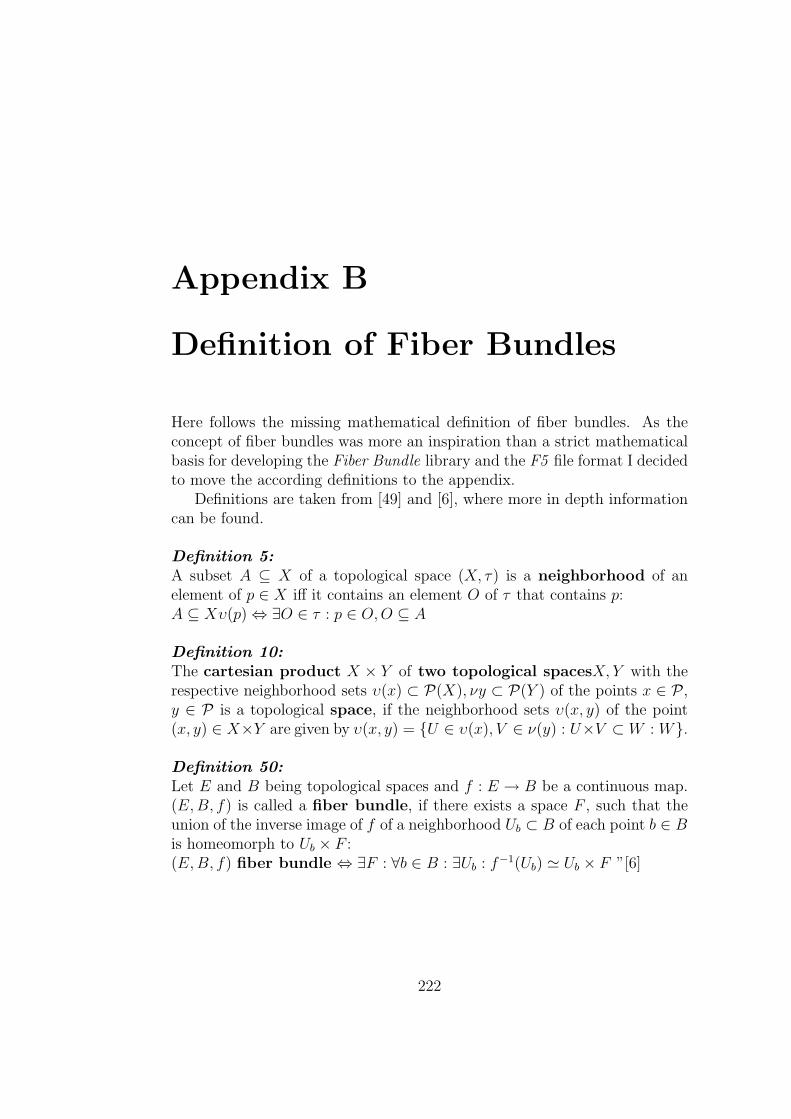
Appendix B
Definition of Fiber Bundles
Here follows the missing mathematical definition of fiber bundles. As theconcept of fiber bundles was more an inspiration than a strict mathematicalbasis for developing the Fiber Bundle library and the F5 file format I decidedto move the according definitions to the appendix.
Definitions are taken from [49] and [6], where more in depth informationcan be found.
Definition 5:A subset A ⊆ X of a topological space (X, τ) is a neighborhood of anelement of p ∈ X iff it contains an element O of τ that contains p:A ⊆ Xυ(p)⇔ ∃O ∈ τ : p ∈ O,O ⊆ A
Definition 10:The cartesian product X × Y of two topological spacesX, Y with therespective neighborhood sets υ(x) ⊂ P(X), νy ⊂ P(Y ) of the points x ∈ P ,y ∈ P is a topological space, if the neighborhood sets υ(x, y) of the point(x, y) ∈ X×Y are given by υ(x, y) = U ∈ υ(x), V ∈ ν(y) : U×V ⊂ W : W.
Definition 50:Let E and B being topological spaces and f : E → B be a continuous map.(E,B, f) is called a fiber bundle, if there exists a space F , such that theunion of the inverse image of f of a neighborhood Ub ⊂ B of each point b ∈ Bis homeomorph to Ub × F :(E,B, f) fiber bundle ⇔ ∃F : ∀b ∈ B : ∃Ub : f−1(Ub) ' Ub × F ”[6]
222

Appendix C
Related Publications
During the work on the thesis I was involved in four related publications: [1],[12], [10] and [16]. I participated at the WSCG (Winter School of ComputerGraphics, [53]) in Plzen, Czech Republic in 2009 and 2010 and presented thecommunication paper [1] during the conference.The publications are included here in the appendix.
223

Fiberbundle-Based Visualization of a Stirred-Tank Flow
Werner Benger
Feng Jijao Center for Computation &
Technology at Louisiana State University
239 Johnston Hall USA, LA 70803, Baton Rouge
[email protected] [email protected]
Marcel Ritter Center for Computation &
Technology at LSU and
Department of Computer Science University of Innsbruck Technikerstrasse 21a
Austria, A-6020 Innsbruck [email protected]
Sumanta Acharya Somnath Roy
Louisiana State University Department of Mechanical
Engineering USA, LA 70803, Baton Rouge
ABSTRACT We describe a novel approach to treat data from a complex numerical simulation in a unified environment using a generic data model for scientific visualization. The model is constructed out of building blocks in a hierarchical scheme of seven levels, out of which only three are exposed to the end-user. This generic scheme allows for a wide variety of input formats, and results in powerful capabilities to connect data. We review the theory of this data model, implementation aspects in our visualization environment, and its application to computational fluid dynamic simulation of flow in an impeller-stirred tank. The computational data are given as a velocity vector field and a scalar pressure field on a mesh consisting of 2088 blocks in curvilinear coordinates.
Keywords Computational fluid dynamics, data model, stream lines, scientific visualization.
1 INTRODUCTION Computational fluid dynamics (CFD) has advanced significantly in the last few years and can now provide high fidelity temporally and spatially resolved numerical data. This data is based on meshes that range from a few million cells to tens of million cells, and for several hundred thousand time steps, with data files that are of the order of terabytes. A key challenge therefore is the ability to easily and cost-effectively mine this data for key features of the flow field and to display these spatially evolving features in the space-time domain of interest. In this work, we present an integrated interdisciplinary effort that takes utilizes of a generic approach to handle scientific data sets leading to new visualization capabilities in a natural way. The CFD dataset is obtained from a large eddy simulation (LES) of flow inside a stirred tank reactor (STR), such as depicted in Figure 1. The STRs are widely used as mixing devices in chemical industry. The STR that we investigated here is a cylindrical
tank with a hemispherical bottom, vertical baffles mounted along the cylindrical walls, and rotating impellers consisting rectangular blades with 45° pitch angle mounted on a shaft passing through its center, see Figure 2. As the impeller rotates, its blades pump the fluid axially downward towards the bottom of the tank. The fluid-jet then
hits the hemispherical bottom wall and sets in a circulating motion of fluid within the tank promoting mixing between the top and the bottom of the tank.
Figure 1: Stir Tank (Courtesy Dow Chemicals)
The calculations are done on a multi-block curvilinear mesh as shown in Figure 3. Calculations are done on nearly three million cells using a multi-block body fitted finite volume flow solver. Since the tank contains a set of impeller blades that are rotating and also contains stationary
Permission to make digital or hard copies of all or part of this work for personal or classroom use is granted without fee provided that copies are not made or distributed for profit or commercial advantage and that copies bear this notice and the full citation on the first page. To copy otherwise, or republish, to post on servers or to redistribute to lists, requires prior specific permission and/or a fee.
Figure 2: Impeller geometry

features such as baffles on the outer walls, special algorithms (Immersed Boundary Methods) are used to accommodate moving interfaces. The method intrinsically uses a fixed curvilinear mesh fixed to the stationary features of the geometry and tracks or flags the location of the nodes adjacent to the moving surfaces or boundaries. At these flagged nodes, forcing terms/interpolations are performed to satisfy the boundary conditions at the moving surfaces. This approach has been extensively tested in an earlier communication [TRHA07] where computational solution for a similar stirred tank flow has been validated with experimental observations. The visualizations presented here show the axial pumping as well as the circulation zones suggesting the mechanisms of fluid mixing inside the tank. As the impeller blade moves, the fluid jet stream coming out of the top and side wall of the impeller blade interact with each other to form a vortical motion following which fluid elements move in azimuthal direction [RA07]. These vortex structures are identified from the existences of pressure minima. While traditional commercial visualization packages such as Tecplot (www.tecplot.com) and Ensight (www.ensight.com) are commonly used for visualization, they have inherent limitations. It is therefore important to be able to develop sophisticated visualization capabilities that allow a variety of features and controls not commonly available with the commercial software. The VISH visualization environment [BRH07] employed here has been designed to allow a step in this direction.
2 DATA MODEL CONCEPT “A common denominator for scientific data already exists, we just have to use them.” was the paradigm under which Butler & Pendley [BP89] proposed the mathematics of fiber bundle as a foundation for a data model that is able to describe all cases needed for scientific visualization in a common way, since the mathematics behind all the different implementation is an universal language of science
already. Yet a common data model has hardly been used, with the IBM Data Explore one of the few exceptions. The idea of using a fiber bundle as inspiration for a common data model has been revived by Benger [Ben04] to handle the complexity of data stemming from general relativity. These concepts have been built upon and further refined by Heinzl [HEI07] to develop generic software components. In these approaches, concepts have been based on the mathematics of topology and differential geometry to describe data sets.
2.1 Mathematics of Fiber Bundles A fiber bundle is in the mathematical sense is set of a total space E and a base space B with a projection map f such that the union of fibers of a neighborhood U of each point of B is homeomorphic to U×F with F the so called fiber space and the projection of U×F is U again. It is also said that the space F “fibers” over the base space B. If the total space E can be written globally as E=B×F, then E is called a “trivial bundle”. The paradigm is that numerical data sets that are usually needed for scientific visualization can be formulated as trivial bundles. In practice it means that we may distinguish data sets by their properties in the base space and the fiber space. At each point of the – discretized – base space we have some data in the fiber space attached.
Figure 3: Boundaries of the 2088 curvilinear blocks of the computational mesh
The structure of the base space is described as a CW-complex, which categorizes the topological structure of an n-dimensional base space by a sequence of k-dimensional skeletons, with the dimensionality of the skeletons ranging from zero to n. These skeletons carry certain properties of the data set: the 0-skeleton describing vertices, the 1-skeleton the edges, 2-skeleton the faces, etc., of a triangulation of some mesh. For structured grids the topological properties are given implicitly. The structure of the fiber space is (usually) not discrete and given by the properties of the geometrical object residing there, such as a scalar, vector, co-vector, tensor. Same as the base space, the fiber space has a specific dimensionality, though the dimensionality of the base space and fiber space is independent. If the fiber space has vector space properties, then the fiber bundle is called a vector bundle. The most simple vector bundle is the tangential bundle of a manifold, which consists of the manifold as base space and the space of tangential vectors at each point. With n the dimensionality of the manifold, the dimension of the tangential bundle is 2n. Basically a fiber bundle is a set of points with neighborhood information attached to each of them. An n-dimensional array is a very simple case of a fiber bundle (with neighborhood information given implicitly).

2.2 Benefits of Fiber Bundles The concept of a fiber bundle leads to a natural distinction of data describing the base space and data describing the fiber space. This distinction is not common use in computer graphics, where topological properties (base space) are frequently intermixed with geometrical properties (coordinate representations). Operations in the fiber space can however be formulated independently from the base space, which leads to a more reusable design of software components. Coordinate information, formally part of the base space, can as well be considered as fiber, leading to further generalization. The data sets describing a fiber are ideally stored as contiguous arrays in memory or disk, which allows for optimized array and vector operations. Such a storage layout turns out to be particularly useful for communicating data with the GPU using vertex buffer objects: fibers are basically vertex arrays in the notation of computer graphics.
2.3 The 7-Level Hierarchy In the data model implementation of [Ben04] data are formulated in a graph of maximally seven levels, each level representing a certain property of the entire data set. These levels, constituting a “Bundle”, are:
1. Slice 2. Grid 3. Skeleton 4. Representation 5. Field 6. (Fragment) 7. (Compound Elements)
Actual data arrays are stored only below the “Field” level. An actual data set is described by which data sets exist in which level. The actual meaning of each level is described elsewhere [Ben04], [BRH07], [Ben08]. Only two of these hierarchy levels are exposed to the end-user, these are the “Grid” and “Field” levels.
2.4 Bundles, Grids and Fields An entire dataset, including all time steps or any information given on a parameter space in general, is denoted as a Bundle, following the mathematical term of a fiber bundle. The objective is to formulate all data that is used for scientific visualization within this Bundle. A Grid is subset of data within the Bundle that refers to a specific geometrical entity, for instance a mesh carrying data such as a triangular surface, a data cube, a set of data blocks from a parallel computation, etc. A Field is the collection of data sets given as numbers on a specific topological
component of a Grid, for instance floating point values describing pressure or temperature. The names of Grids and Fields are arbitrary and specified by the user. All other levels of the data model have pre-defined meanings and values which are used internally to describe the properties of the Bundle as construction blocks. The usage of these construction blocks constitutes a certain language to describe a wide range of data sets. For instance, a Slice is identified by a single floating point number representing time (generalization to arbitrary-dimensional parameter spaces is possible); a Skeleton is identified by its dimensionality, index depth (relationship to the vertices of a Grid) and refinement level; a Representation is identified via some reference object, which may be some coordinate system or another Skeleton. The meaning of such identifiers is only used internally, but transparent to the user. The lowest levels of Fragments and Compound describe the internal memory layout of a Field data set and are optional. They are described in detail in [Ben08].
2.5 Formulating Data The existence of data sets in the hierarchy of a Bundle defines a data set. We will give some examples here on the data sets that have been involved in our work with the stir tank computational fluid dynamics data.
2.5.1 Isosurface An isosurface is the explicit polygonal representation of the points where a possibly time-dependent scalar field given on a volumetric manifold has constant value. It consists of the following properties:
1. A sequence of Grids, one for each time step 2. Coordinates for each vertex, which is a field
on the Skeleton of index depth 0 (“Vertices”) on each grid, as represented in Cartesian coordinates.
3. Connectivity information for each triangle, which is a field on the Skeleton of dimension 2 and index depth 1 (faces) on each Grid, as represented in the Vertices.
4. Normal vectors define a vector field (precisely: a bi-vector or co-vector field) given on the Vertices Skeleton of the Grid.
5. Optional data fields on the vertices, such as another 3D field mapped on the surface.
An Isosurface is a sequence of Grid objects with two Skeletons defined on it, with the Skeleton for the Vertices carrying two or more fields.

2.5.2 Line Set A set of lines, such as the result of the computation of stream lines of a vector field, is given by
1. A sequence of Grids, one for each time step, for the set of lines valid at each time step
2. Coordinates for each point along the lines, a field on the Skeleton of index depth 0
3. Connectivity information for the points building up a line, which is a field on the Skeleton of dimension 1 and index depth 1 (edges).
4. Tangential vectors define a vector field given on the Vertices Skeleton of the Grid
5. Optional data fields on the vertices may exist, as retrieved from a 3D field mapped on the surface.
A set of lines is very similar to an isosurface in this data model, though a different Skeleton on the Grid objects is employed.
2.5.3 Multiblock Data The numerical data as provided by the computational fluid simulation are given as a collection of 2088 three-dimensional arrays describing coordinate location, pressure and fluid velocity for each grid point. These fields are all fibers on the vertices in the fiber bundle data model, where we also treat the coordinates as a field over the vertices. As the topological structure is regular the edges and faces are given implicitly. The decomposition of the data into blocks is represented as the internal memory layout structure of the fields, thus as field fragments visible in the 6th level of the data hierarchy. The topological structure of the blocks is thereby transparent to the user, but algorithms operate on collections of arrays instead of contiguous arrays, which is relatively straightforward extension to existing algorithms such as the computation of isosurfaces. To store information that is specific to each block, we consider each block as a collection of volume cells. Volume cells are topologically 3-Skeletons in a triangulation, and of index depth 1 in the fiber bundle data model. Collections of such elements are thus of index depth 2. Fibers on this Skeleton are thus a natural place to store e.g. the geometrical bounding box information for a block, or the min/max data range of a scalar field (which speeds up repeated isosurface computations) The layout of a multiblock data set thus consists of:
1. A sequence of Grid objects, one for each time step
2. A coordinate field on the Vertices Skeleton, which is shared among all time steps if the geometry remains constant over time
3. A scalar field on the Vertices Skeleton
4. A vector field on the Vertices Skeleton 5. A Skeleton of dimension 3 and index depth
2 describing a collection of volume elements, which are the respective blocks.
6. Optional scalar fields on the (3,2) Skeleton with min/max information of a scalar field per block, or coordinate fields for bounding box.
2.6 Data Operations Given the certain components constituting the data model, we may formulate abstract operations among such components. These operate on abstract high-level objects without requirement to know the internal structure of the objects, though their concrete implementation will have to deal with them.
2.6.1 Isosurface Computation The computation of an isosurface is an operation that takes a Field as input and yields a Grid object, and will be called for each instance of a time sequence. The operation is parameterized by some isolevel value. Certain conditions must be fulfilled by the input field for this operation to succeed, such as being a scalar-valued field residing on a regular grid. However, more advanced implementations rather than the standard marching cubes may well be formulated through the same interface, such as direct computation of magnitude isolevels of vector fields, or isosurface computation on tetrahedral grid. The high-level operation
Grid = ComputeIsosurface(Field, float);
remains the same, and no changes in the user interface are required. For instance, more advanced operations could be invoked via some runtime plugin mechanism, transparent to the user, as it is supported by VISH.
2.6.2 Grid Evaluation Given Field data on one Grid instance, like a 3D volume, they may be evaluated on another Grid, like a surface or a line set. Such is formulated as an EvalGrid operation which requires specification of a destination grid and a source field (implicitly given on another Grid object):
Field = EvalGrid(Grid Dest, Field Source);
Certain constraints may apply to the input Grid, since the evaluation of a field is not possible on an arbitrary Grid. For instance, data given on a surface cannot be uniquely extrapolated into an entire 3D volume. However, a wide range of operations can be specified through this common API.

3 STREAMLINE STRATEGIES Visualizing vector fields is a common need in CFD for investigating velocity fields. [LaH05] describes several tools for investigating CFD data. [PWS06] shows the combination of different geometry based and texture based techniques in a CFD application. More applications of texture based vector field visualization can be found in [LEG]. With more complicated and large data sets it is increasingly important to have a variety of tools for feature extraction and data exploration at hand. Thus, developing a flexible framework seems the right way to meet the increasing requirements effectively. We use streamlines in our approach because it is a well known standard technique and they can be described well within the context of fiber bundles. The challenge here was to deal with the multi-block curvilinear data structure (as shown in Figure 3) and to verify the applicability of the Fiber Bundle data model. Using this model, our streamline visualization implementation modules separate into four groups: Vector Field Data, Seed Point Data, Streamline Computation and Line Rendering. The software modules are connected in a directed graph communicating data using Grids and Fields. This allows to exchange modules by other modules (high reusability) and to combine modules in different ways (high flexibility).The Streamline Computation Module takes a vector Field and an arbitrary Grid defining the seed points as inputs and outputs a Line Set as Grid.
This allows to exchange modules by other modules (high reusability) and to combine modules in different ways (high flexibility).The Streamline Computation Module takes a vector Field and an arbitrary Grid defining the seed points as inputs and outputs a Line Set as Grid.
The computation of the streamline involves finding the location of a given world position in the dataset by identifying its block, cell and local curvilinear cell coordinates. These local coordinates are then used for linear interpolation of the vector field. The interpolated vector is used to advance to the next streamline point of the streamline, another world position.
The computation of the streamline involves finding the location of a given world position in the dataset by identifying its block, cell and local curvilinear cell coordinates. These local coordinates are then used for linear interpolation of the vector field. The interpolated vector is used to advance to the next streamline point of the streamline, another world position. Firstly, a kD-Tree is employed to find blocks, which might contain the world position, secondly a look up data structure called UniGridMapper that maps a uniform grid cell to curvilinear cells that might contain the world position is used and finally a Taylor approximation and Newton iteration, as described in [STA98], retrieves the local curvilinear cell coordinates.
Firstly, a kD-Tree is employed to find blocks, which might contain the world position, secondly a look up data structure called UniGridMapper that maps a uniform grid cell to curvilinear cells that might contain the world position is used and finally a Taylor approximation and Newton iteration, as described in [STA98], retrieves the local curvilinear cell coordinates. Besides storing the calculated stream lines as Line Sets in the output Grid additional Fields are stored that carry the information necessary for interpolation. Block IDs and local cell coordinates are stored. This information can then be used by other independent modules to evaluate other data Fields on the streamline Grid, e.g. to evaluate a pressure Field. The final Line Rendering module employs illuminated stream lines, similar to those described in [SZH97]
Besides storing the calculated stream lines as Line Sets in the output Grid additional Fields are stored that carry the information necessary for interpolation. Block IDs and local cell coordinates are stored. This information can then be used by other independent modules to evaluate other data Fields on the streamline Grid, e.g. to evaluate a pressure Field. The final Line Rendering module employs illuminated stream lines, similar to those described in [SZH97]
3.1 Defining Seed Point for Streamlines 3.1 Defining Seed Point for Streamlines To visualize the characteristics of a certain vector field by streamlines it is important to find good starting points (seed points) for the streamline integration.
To visualize the characteristics of a certain vector field by streamlines it is important to find good starting points (seed points) for the streamline integration.
3.1.1 Grid Convolver 3.1.1 Grid Convolver An operation called Grid Convolver allows the user to create sophisticated seed point geometries by ‘convoluting’ vertices of an input Grid with a set of parameters into an output Grid, similar to the mathematical convolution operation. Possible Grid convolution operations are Point, Line, Rectangle, Circle, Ellipsoid and Uniform Grid.
An operation called Grid Convolver allows the user to create sophisticated seed point geometries by ‘convoluting’ vertices of an input Grid with a set of parameters into an output Grid, similar to the mathematical convolution operation. Possible Grid convolution operations are Point, Line, Rectangle, Circle, Ellipsoid and Uniform Grid. Figure 5 demonstrates a setup for creating seed points involving three Grid Convolvers. The first Grid Convolver(a) gets one point as input Grid. It ‘convolutes’ this input on a vertical Line with a subdivision of three points. This is then outputted into the second Grid Convolver(b) which ‘convolutes’ the three-point-Line on its horizontal two-point-Line. This results in the output Grid seen in (c). A final Grid Convolver(d) now ‘convolutes’ on its Circle geometry resulting in the final seed points in the output Grid of (d), shown in (e).
Figure 5 demonstrates a setup for creating seed points involving three Grid Convolvers. The first Grid Convolver(a) gets one point as input Grid. It ‘convolutes’ this input on a vertical Line with a subdivision of three points. This is then outputted into the second Grid Convolver(b) which ‘convolutes’ the three-point-Line on its horizontal two-point-Line. This results in the output Grid seen in (c). A final Grid Convolver(d) now ‘convolutes’ on its Circle geometry resulting in the final seed points in the output Grid of (d), shown in (e). Since the module can be connected to any other modules that output Grid objects it is possible to create many different seed geometries. The module thus is highly reusable and flexible. Figure 4 illustrates a typical dataflow involving Field and
Since the module can be connected to any other modules that output Grid objects it is possible to create many different seed geometries. The module thus is highly reusable and flexible. Figure 4 illustrates a typical dataflow involving Field and
In: Grid
Out: Grid
In: Bundle
Out: Grid
In: Grid
Out: Field In: Field
Out: Grid
In: Grid
Out: Grid
In: Grid
F5 Data Bundle
Grid Selector
Vector Field
Grid Convolver
Streamlines Computation
Input - Grid
In: Grid
Line Renderer
… Out: Grid
Grid Convolver
Figure 4: Streamline modules and dataflow

Grid objects. Figure 6, 7, and 8 demonstrate how this module was used to investigate the stir tank velocity field with different settings of position and rotation and different number of connected Grid Convolvers.
Figure 6: Streamlines with seed points on a circle.
Figure 7: Streamlines emitted from seed points on a circle of circles of lines by using three Grid Convolvers.
Figure 8: Streamlines emitted on an array of lines.
Figure 9: Space-filling streamlines in the STR
Besides interactively specifying seed points it is also possible to utilize other seeding methods such as those found in AMIRA [SWH05], where a threshold on a scalar field can specify seed points for a vector field, or similar to Weinkauf’s method of computing the curvature measures of a vector field to find critical regions as indicators where streamlines were most interesting [WTH02]. Even a full coverage of the entire volume may provide worthwhile information (Figure 9).
3.1.2 Seed Points by Iso Surfaces The usage of a Grid input at the Streamline Computer allows usage of arbitrary compatible Grid objects for defining seed points. For example, the Grid of an iso surface (the vertices of the triangular surface) computed on the pressure scalar field can be used as input, as shown in Figure 9 and Figure 10. With such streamline seeding the vector field close to the surface can be explored, similar to a texture based technique applied to the surface such as [LSH04]. This is a unique feature of VISH that can potentially be exploited to better understand the flow physics.
a) b)
c) d)
e) Figure 5: Example of
constructing seed points by connecting three
Grid Convolver modules a), b) and d).

4 PERFORMANCE RESULTS Computation of 100 streamlines in the given multiblock dataset of 2088 curvilinear blocks required about 7 seconds using an Euler integration scheme for 100 steps on a Intel Xeon CPU, 2.5GHz. Tecplot required 35 seconds using a comparable setup. We could not compare with Amira, since this data type is not supported there. The computation time of the isosurface crucially depends on the chosen level, and is below 1/30th second for most values, but may require up to 2 seconds in particular cases. Computing streamlines from the isosurface vertex requires about 5-10 seconds for the setup as shown in Figure 11, but will linearly depend on the chosen length. Future improvements will utilize higher order integration schemes and parallelization, for which we expect to be able to reduce computation times under one second. The frame rates for rendering itself once the streamlines are computed are under 1/30th of a second in all cases except Figure 9, where we got about 10 frames per second on an NVidia Quadro FX 5600 graphics board.
5 DISCUSSION
Figure 10: Detail of the emission of streamlines from the pressure isosurface. Figure 10 shows velocity vectors adjacent to the impeller blades. It can be clearly seen that as the impeller rotates in the clockwise direction, the pitched blade surfaces force the fluid in its surface-normal direction imposing both radially outward and downward velocities on the flow along with an azimuthal velocity component due to its rotation. The pressure isosurface depicts the boundary layer formed over the impeller blade surface and its evolution downstream. Circular depressions (marked as P in Figure 11) can be observed in the pressure isosurface. These depressions point to local pressure minima suggesting formations of vortical structures in the direction opposite to the impeller rotation. These vortices (commonly termed as trailing-edge
vortices) convect fluid in the azimuthal direction and play a key role in mixing within the tank.
Figure 11: Velocity micro-streamlines and
pressure isosurfaces over the impeller blade Figure 12 shows the streamlines coming out of an impeller blade. The downward pumping from the impeller is clearly observable. Also, the streamlines are observed to bend near the hemispherical bottom of the tank and establish a circulating motion. The colors along the streamlines indicate the residence time of the fluid particles. The suction of the upper fluid is identified by the green color, the yellow colored impeller jet stream has both radial and axial component as the streamlines show almost a 45° bend. Later (orange color) these lines hit the bottom of the tank and bend upwards (red coloration) and the fluid is again convected to the upper part of the tank. This circulation is how the fluid mixing operation takes place in the stirred tank.
Figure 12: Streamlines over the tank volume

6 SUMMARY We have described and applied the concept of “Grid objects” as elementary tools within a highly modular visualization environment to provide powerful seeding mechanisms for streamline computation to visualize flow in a stirred tank. Operations such as “Grid convolution” and seeding by pressure isosurfaces are natural consequences of utilizing the described data model. It is argued here that this approach offers specific capabilities that several other visualization platforms are unable to provide.
7 ACKNOWLEDGMENTS This research employed resources of the Center for Computation & Technology at LSU, which is supported by funding from the Louisiana legislature's Information Technology Initiative. Portions of this work were supported by NSF/EPSCoR Award No. EPS-0701491 (CyberTools). We thank Georg Ritter for his industrious work on the VISH infrastructure.
8 REFERENCES [Ben04] Benger, W. Visualization of General
Relativistic Tensor Fields via a Fiber , PhD - thesis FU Berlin, 2004
[BRH07] W. Benger, G. Ritter and R. Heinzl, The Concepts of VISH, Proc. 4th High End Visualization Workshop Obergurgl, p. 26-39, 2007, Lehmann’s Media
[Ben08] Benger, W. Colliding galaxies, rotating neutron stars and merging black holes - visualizing high dimensional data sets on arbitrary meshes, New J. Phys. 10 (2008) 125004, http://stacks.iop.org/1367-2630/10/125004.
[BP89] O. Butler, D. M. & Pendley, M. H. (1989). A visualization model based on the mathematics of fiber bundles. Comp. in Physics, 3(5), 45-51.
[HEI07] R. Heinzl: "Concepts for Scientific Computing"; PhD Thesis; Institut für Mikroelektronik, TU Wien, 2007;
[LaH05] Robert S. Laramee & Helwig Hauser, Interactive 3D Flow Visualization Based on Textures and Geometric Primitives, in NAFEMS World Congress Conference Proceedings, The International Association for the Engineering Analysis Community, May 17-20, 2005, St. Juliens Bay, Malta
[LEG] R. S. Laramee, G. Erlebacher, C. Garth, T. Schafhitzel, H. Theisel, X. Tricoche, T. Weinkauf, D. Weiskopf, Applications of Texture-Based Flow Visualization, Engineering Applications of Computational Fluid Mechanics, in publication
[LSH04] R. S. Laramee, J. Schneider & H. Hauser: Texture-Based Flow Visualization on Isosurfaces from Computational Fluid Dynamics, Proceedings of the 6th Joint IEEE TCVG - EUROGRAPHICS Symposium on Visualization (VisSym 2004), May 19-21, 2004, Konstanz, Germany
[MPS05] O. Mallo, R. Peikert, C. Sigg, F. Sadlo, Illuminated Lines Revisited, Proceedings of IEEE Vis 2005, pp. 19-26 (Minneapolis, MN, USA, October 23-28, 2005)
[PWS06] C. Petz, T. Weinkauf, H. Streckwall, F. Salvatore, B.R. Noack, H.-C. Hege, Vortex Structures at a Rotating Ship Propeller, Presented at the 24th Annual Gallery of Fluid Motion exhibit, held at the 59th Annual Meeting of the American Physical Society, Division of Fluid Dynamics, Tampa Bay, November 2006
[RA07] S. Roy, and S. Acharya, “Study on Flow and Turbulence Inside a Stirred Tank and Investigation on the Effects of Macroinstability on Trailing Vortex Structures”, ASME International Mechanical Engineering Congress and Exposition, Seattle, November 2007
[STA98] D. Stalling. “Fast texture-based algorithms for vector field visualization.” Dissertation, FU Berlin, Preprint SC-98-58, Konrad-Zuse-Zentrum Berlin (ZIB), December 1998.
[SWH05] D. Stalling and M. Westerhoff and H.-C. Hege, “Amira - an object oriented system for visual data analysis”, Visualization Handbook, Christopher R. Johnson and Charles D. Hansen, Academic Press, 2005
[SZH97] D.Stalling, M.Zockler, and H.-C. Hege. Fast display of illuminated field lines. In IEEE Transactions on Visualization and Computer Graphics, vol.3, pages 118-128, 1997.
[SZH97] D.Stalling, M.Zockler, and H.-C. Hege. Fast display of illuminated field lines. In IEEE Transactions on Visualization and Computer Graphics, vol. 3, pages 118-128, 1997.
[TRHA07] M. Tyagi, S. Roy, S. Acharya, and A-D Harvey III, “Simulation of laminar and turbulent impeller stirred tanks using immersed boundary method and large eddy simulation technique in multi-block curvilinear geometries”, Chemical Engineering Sciences, volume 63, issue 5, pages 1351-1363, 2007
[WTH02] T. Weinkauf, H. Theisel, Curvature Measures of 3D Vector Fields and their Applications, Journal of WSCG 10(2), WSCG 2002, Plzen, Czech Republic, February 4 - 8, 2002

Beyond the Visualization Pipeline:
The Visualization Cascade
Werner Benger1 and Georg Ritter2 andMarcel Ritter1,3 and Wolfram Schoor3
1Center for Computation and Technology, Louisiana State University, USA2Institute for Astro- and Particle Physics, University of Innsbruck3Institute of Computer Science, University of Innsbruck, Austria
4Fraunhofer Institute for Factory Operation and Automation
[email protected], [email protected],[email protected], [email protected]
Abstract
The concept of a pipeline has become a quite common way of thinkingabout the process of visualizing data. In this article we discuss the inher-ent limits of this concept and argue for the need to expand this conceptfor achieving higher performance and convenience to the end user. Whilethe traditional model of a visualization pipeline describes the executionof some data flow, it is most suitable for a static data-set. However fortime-dependent data (e.g.) we intend visualizations to be as fast in timeas they are in space. The pipeline model does not recognize similarity andrepetition of operations which is essential to achieve the desired perfor-mance. The pipeline model thus needs to be extended to efficiently covermultiple traversals and caching of intermediate results, which we call theVisualization Cascade. It will be demonstrated in practice within its im-plementation in the VISH visualization environment.
1 Introduction
The process of visualizing data begins with the source data containing the in-formation to be visualized and ends, finally, with a derived image representingthe data. To arrive at the image the data needs processing, like being searchedor filtered, depending on the nature of the data and the analysis requirements.It then must be mapped to graphical entities that are subsequently renderedinto an image. In [Haber & McNabb, 1990] the authors identify and refinethe general operations data undergoes in the process of creating visualization.The data flows in a pipeline through a chain of stages, as depicted in Fig-ure 1, and finally, results in a representing image. The pipelined model theypresent, is known as the Haber-McNabb model of the visualization pipeline and

has been a widely successful concept for the design of visualization software.Several well known software packages have been built upon this idea, exam-ples include AVS [Upson et al., 1989], VTK [Schroeder et al., 1997], IRIS Ex-plorer [Foulser, 1995], OpenDX [Treinish, 1997] (for a more complete list see[A.A. Ahmed, 2007]).
Data Source
Dataflow
Enrichment/Enhancement
DerivedData
AbstractViz Object Image
Viz Mapping Rendering
Figure 1: Visualization Pipeline: Data flows through the pipeline while opera-tors modify the stream. They extract, filter, map and render data. Finally thepipeline outputs is an image or image stream.
While trying to understand the data through exploratory visualization, asoutlined in [Upson et al., 1989, Card et al., 1999], a flexible and easy to usemechanism to enter the operation on the data into the software is needed. Ex-ploring and trying to understand as much as possible from the data by inspect-ing them, includes making frequent changes to parameters of the visualization,sometimes even to the parameters or models used to create the data. Being ableto easily change and adapt the parameters and, in addition, derive the visualiza-tion results fast, is of great importance as it helps to decrease the time neededfor one investigative cycle. For some data, features might only become visible ifit is possible to navigate interactively inside the parameter space.
The pipeline concept has been found to be well suited and intuitive to under-stand when used to represent the flow of data in a user interface. The user cangraphically construct a visualization pipeline by interconnecting different stagesthrough attaching a pipeline to nodes. An early example of such a graphicallyprogramming interface has been implemented in ConMan [Haeberli, 1988], moremodern examples include the Spiegel framework [Bischof et al., 2006], or thegraphical user interface of LabVIEW [Johnson & Jennings, 2001] in which adata stream, mainly originating from measurements, can be connected to pro-cessing nodes or the gstreamer framework [Black et al., 2002] in which multi-

media data is handled this way.Once the structure of the pipeline has been set up, it needs to be executed.
Different schemes have been implemented to derive the final image. When us-ing implicit execution, as applied in VTK [Schroeder et al., 1997], data is timestamped and only “upstream” nodes are executed, if demanded. Explicit execu-tion, as used in the IRIS Explorer [Foulser, 1995], relies on external managementof the data processing nodes to decide which needs re-computation.
The flow of data is initiated in two principal ways. In the “pull” case, adownstream receiver requests the data from an “upstream” node. In a “push”case, the “upstream” node would forward the data to the next stage in thepipeline as soon as it is available. Also a mixed version can be implemented, asthey are independent.
If we want achieve full interactivity in the visualization of large data-setswe find that the current design of pipelines and their execution models are notwell suited to meet the requirements. Response times to changes of parametersare not fast enough, as data travels too slowly through the whole pipeline toreach an interactive frame rate, as described in [Shen, 2006] for the case of timedependent data.
Not only for a change in the time parameter, but for any change madeto a parameter of the visualization, the whole visualization pipeline has to beexecuted for every single frame. As this often exceeds the time required foran interactive frame rate, a common solution is to apply off-line rendering.Frames of an animation sequence are rendered for later viewing, but interactivelyexploring the data would be more desirable and would also possibly increase thechance of gaining further understanding of for example spatial-temporal featuresof the data.
Working toward the visualization challenges one (“Make the spatial and tem-poral resolution of visual displays indistinguishable from physical reality.”) andfour (“Optimize physical resources used to perform visual interactions.”), as de-scribed in [Hibbard, 1999] and incorporating the user wishes for interactivity,here we present an extended pipeline model that utilizes the structure of mod-ern graphics hardware to minimize the time needed to derive the final image.We propose that, by introducing a flexible caching mechanism, it is possibleto increase re-usage of already processed data, especially in between differentpipelines constructed for different parameter sets. In combination with a datastorage model and utilizing GPU memory, full interactivity on a data-set of thesize of 17 GB, containing 1.6 million points in 200 time steps [Benger, 2008],has been achieved.
2 The Visualization Cascade
The major drawback of the concept of the visualization pipeline is that it doesnot talk about caching of results. If an operation similar to an earlier is to berepeated, we would not want to have the entire pipeline to be traversed again.Only those sections that have changed shall be re-computed. A typical usage
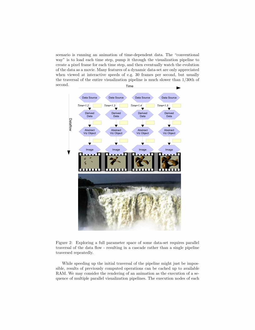
scenario is running an animation of time-dependent data. The “conventionalway” is to load each time step, pump it through the visualization pipeline tocreate a pixel frame for each time step, and then eventually watch the evolutionof the data as a movie. Many features of a dynamic data-set are only appreciatedwhen viewed at interactive speeds of e.g. 30 frames per second, but usuallythe traversal of the entire visualization pipeline is much slower than 1/30th ofsecond.
Data Source
Time
DerivedData
AbstractViz Object
Image
Dataflow
Time=1.2
Data Source
DerivedData
AbstractViz Object
Image
Time=1.3
Data Source
DerivedData
AbstractViz Object
Image
Data Source
DerivedData
AbstractViz Object
Image
Time=1.4 Time=1.5
Figure 2: Exploring a full parameter space of some data-set requires paralleltraversal of the data flow - resulting in a cascade rather than a single pipelinetraversed repeatedly.
While speeding up the initial traversal of the pipeline might just be impos-sible, results of previously computed operations can be cached up to availableRAM. We may consider the rendering of an animation as the execution of a se-quence of multiple parallel visualization pipelines. The execution nodes of each
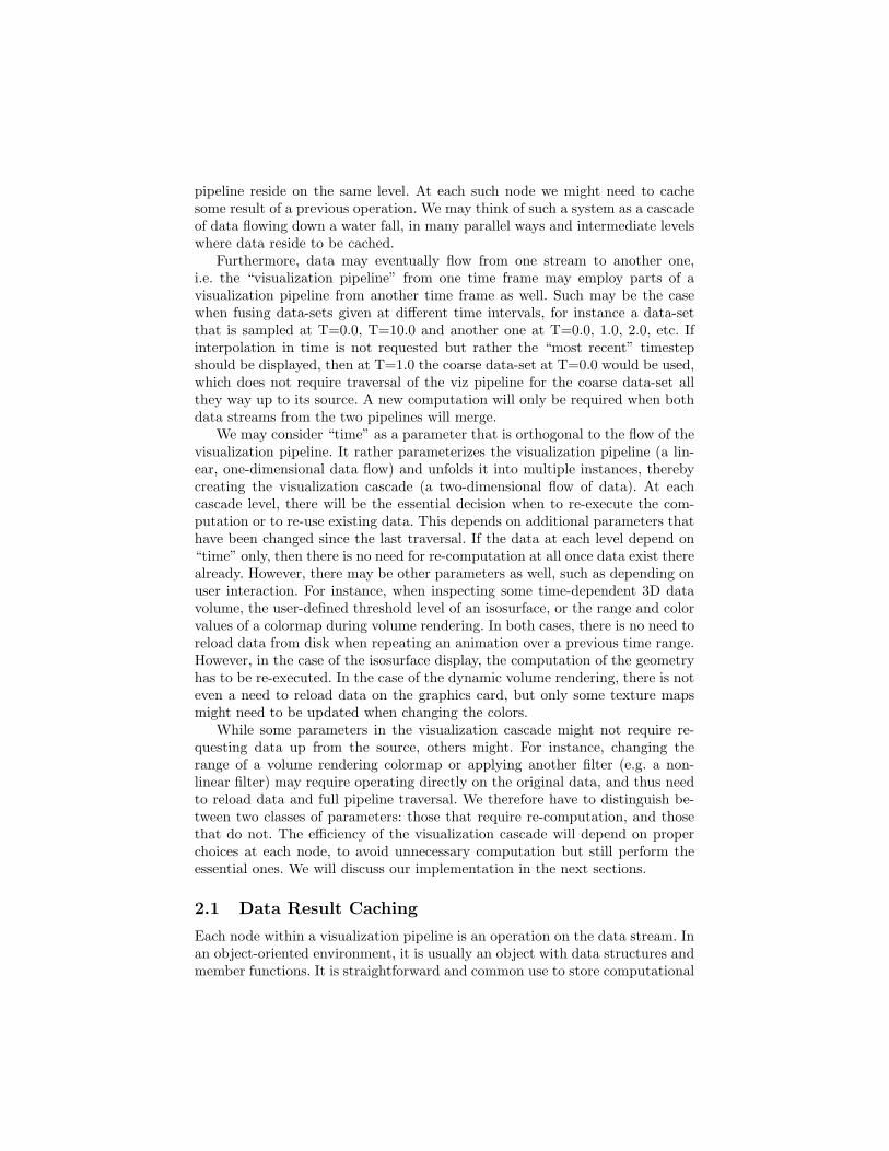
pipeline reside on the same level. At each such node we might need to cachesome result of a previous operation. We may think of such a system as a cascadeof data flowing down a water fall, in many parallel ways and intermediate levelswhere data reside to be cached.
Furthermore, data may eventually flow from one stream to another one,i.e. the “visualization pipeline” from one time frame may employ parts of avisualization pipeline from another time frame as well. Such may be the casewhen fusing data-sets given at different time intervals, for instance a data-setthat is sampled at T=0.0, T=10.0 and another one at T=0.0, 1.0, 2.0, etc. Ifinterpolation in time is not requested but rather the “most recent” timestepshould be displayed, then at T=1.0 the coarse data-set at T=0.0 would be used,which does not require traversal of the viz pipeline for the coarse data-set allthey way up to its source. A new computation will only be required when bothdata streams from the two pipelines will merge.
We may consider “time” as a parameter that is orthogonal to the flow of thevisualization pipeline. It rather parameterizes the visualization pipeline (a lin-ear, one-dimensional data flow) and unfolds it into multiple instances, therebycreating the visualization cascade (a two-dimensional flow of data). At eachcascade level, there will be the essential decision when to re-execute the com-putation or to re-use existing data. This depends on additional parameters thathave been changed since the last traversal. If the data at each level depend on“time” only, then there is no need for re-computation at all once data exist therealready. However, there may be other parameters as well, such as depending onuser interaction. For instance, when inspecting some time-dependent 3D datavolume, the user-defined threshold level of an isosurface, or the range and colorvalues of a colormap during volume rendering. In both cases, there is no need toreload data from disk when repeating an animation over a previous time range.However, in the case of the isosurface display, the computation of the geometryhas to be re-executed. In the case of the dynamic volume rendering, there is noteven a need to reload data on the graphics card, but only some texture mapsmight need to be updated when changing the colors.
While some parameters in the visualization cascade might not require re-questing data up from the source, others might. For instance, changing therange of a volume rendering colormap or applying another filter (e.g. a non-linear filter) may require operating directly on the original data, and thus needto reload data and full pipeline traversal. We therefore have to distinguish be-tween two classes of parameters: those that require re-computation, and thosethat do not. The efficiency of the visualization cascade will depend on properchoices at each node, to avoid unnecessary computation but still perform theessential ones. We will discuss our implementation in the next sections.
2.1 Data Result Caching
Each node within a visualization pipeline is an operation on the data stream. Inan object-oriented environment, it is usually an object with data structures andmember functions. It is straightforward and common use to store computational
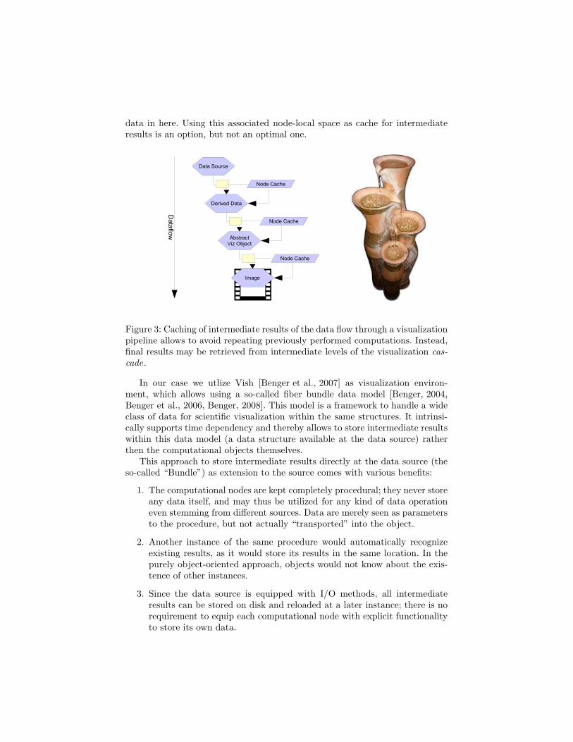
data in here. Using this associated node-local space as cache for intermediateresults is an option, but not an optimal one.
Data Source
Dataflow
Derived Data
AbstractViz Object
Image
Node Cache
Node Cache
Node Cache
Figure 3: Caching of intermediate results of the data flow through a visualizationpipeline allows to avoid repeating previously performed computations. Instead,final results may be retrieved from intermediate levels of the visualization cas-cade.
In our case we utlize Vish [Benger et al., 2007] as visualization environ-ment, which allows using a so-called fiber bundle data model [Benger, 2004,Benger et al., 2006, Benger, 2008]. This model is a framework to handle a wideclass of data for scientific visualization within the same structures. It intrinsi-cally supports time dependency and thereby allows to store intermediate resultswithin this data model (a data structure available at the data source) ratherthen the computational objects themselves.
This approach to store intermediate results directly at the data source (theso-called “Bundle”) as extension to the source comes with various benefits:
1. The computational nodes are kept completely procedural; they never storeany data itself, and may thus be utilized for any kind of data operationeven stemming from different sources. Data are merely seen as parametersto the procedure, but not actually “transported” into the object.
2. Another instance of the same procedure would automatically recognizeexisting results, as it would store its results in the same location. In thepurely object-oriented approach, objects would not know about the exis-tence of other instances.
3. Since the data source is equipped with I/O methods, all intermediateresults can be stored on disk and reloaded at a later instance; there is norequirement to equip each computational node with explicit functionalityto store its own data.
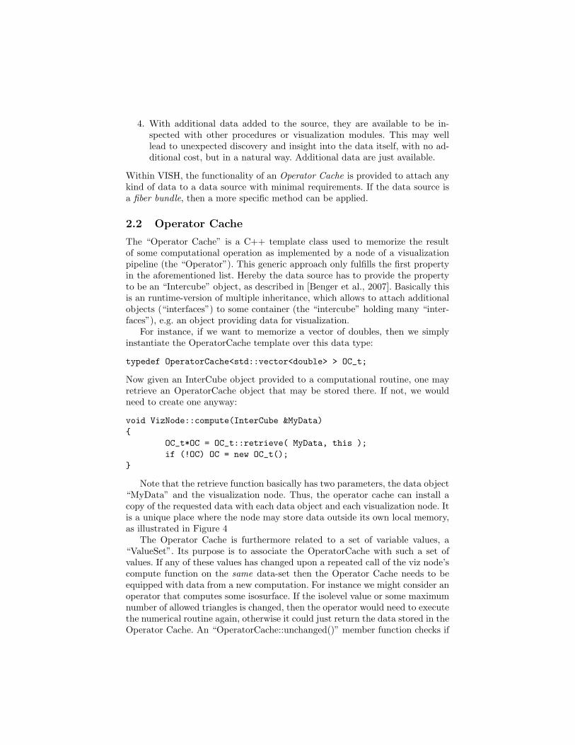
4. With additional data added to the source, they are available to be in-spected with other procedures or visualization modules. This may welllead to unexpected discovery and insight into the data itself, with no ad-ditional cost, but in a natural way. Additional data are just available.
Within VISH, the functionality of an Operator Cache is provided to attach anykind of data to a data source with minimal requirements. If the data source isa fiber bundle, then a more specific method can be applied.
2.2 Operator Cache
The “Operator Cache” is a C++ template class used to memorize the resultof some computational operation as implemented by a node of a visualizationpipeline (the “Operator”). This generic approach only fulfills the first propertyin the aforementioned list. Hereby the data source has to provide the propertyto be an “Intercube” object, as described in [Benger et al., 2007]. Basically thisis an runtime-version of multiple inheritance, which allows to attach additionalobjects (“interfaces”) to some container (the “intercube” holding many “inter-faces”), e.g. an object providing data for visualization.
For instance, if we want to memorize a vector of doubles, then we simplyinstantiate the OperatorCache template over this data type:
typedef OperatorCache<std::vector<double> > OC_t;
Now given an InterCube object provided to a computational routine, one mayretrieve an OperatorCache object that may be stored there. If not, we wouldneed to create one anyway:
void VizNode::compute(InterCube &MyData)
OC_t*OC = OC_t::retrieve( MyData, this );if (!OC) OC = new OC_t();
Note that the retrieve function basically has two parameters, the data object“MyData” and the visualization node. Thus, the operator cache can install acopy of the requested data with each data object and each visualization node. Itis a unique place where the node may store data outside its own local memory,as illustrated in Figure 4
The Operator Cache is furthermore related to a set of variable values, a“ValueSet”. Its purpose is to associate the OperatorCache with such a set ofvalues. If any of these values has changed upon a repeated call of the viz node’scompute function on the same data-set then the Operator Cache needs to beequipped with data from a new computation. For instance we might consider anoperator that computes some isosurface. If the isolevel value or some maximumnumber of allowed triangles is changed, then the operator would need to executethe numerical routine again, otherwise it could just return the data stored in theOperator Cache. An “OperatorCache::unchanged()” member function checks if

InterCube
InterCube
InterCubeData
Operator
Operator
Data
Data
Figure 4: Data Storage in Intercubes
there are any such differences among the values stored with the OperatorCacheand the current values had occured (it will automatically return “false“ if theOperatorCache was newly created):
ValueSet*Changeables = new ValueSet();Changeables->addValue(IsoValue);Changeables->addValue(NumberOfAllowedTriangles);
if (OC->unchanged( Changeables ) )
// do something with the data existing in OCreturn;
// compute new data and put them into the OC
If there had been changes, then following code is supposed to compute newdata. There may be other parameters that do not require re-computation, suchas another coloring of the resulting isosurface, see Figures 5, 6 and 7. These willbe part of the visualization node, but not be added to the ValueSet that is usedto inspect the Operator Cache. (The actual source code uses a slightly differentsyntax as it employs operator overloading to provide a more compact coding.)
2.3 Caching in the Fiber Bundle
When data are available in the fiber bundle, and results are storable in the fiberbundle, one would not employ the OperatorCache. Rather, any results will bestored directly in the incoming data structures. To depict how it works, we donot need to know the entire complexity of the full model. It suffices to know thatthere are objects called Bundle and Grid. A Bundle may be accessed with afloating point value and a string to yield a Grid object. Such a Grid object mayrepresent a 3D data volume with scalar fields (which is to be identified via somestring), or a triangular surface such as the result of an isosurface computation.The actual numerical routine “Isosurface” will require a Grid object, a fieldname, and a floating point value specifying the isolevel. The schematic code willlook similar to this:

Surface RendererColor=Red
...
Rendered Surface
Image
Uniform Scalarfield
IsoSurface ExtractorIsoLevel=0.2
disk
IsoSurfaceScene Compositing
GUI XScene Paramters:
IsoLevel=0.2Color=Red
Figure 5: The execution flow: The first time, the complete cascade has to beexecuted. The operators read the data-set from disk, compute the isosurface,render the surface and composite it to the final image. The separation intooperators is hidden and is not all seen by the user.
Grid VizNode::compute(Bundle&B, double time,string Gridname, string Fieldname,double Isolevel)
// Construct a unique name for the computational result
string IsosurfaceName = Gridname + Fieldname + Isolevel;// Check whether result already exists for the given time
Grid IsoSurface = B[ time ][ IsosurfaceName ];if (!IsoSurface)
// No, thus need to retrieve the data volumeGrid DataVolume = B[ time ][ Gridname ];
// and perform the actual computationIsoSurface = Compute( DataVolume, Fieldname, Isolevel);
// finally store the resulting data in the bundle objectB[ time ][ IsosurfaceName ] = IsoSurface;
return IsoSurface;
Note that in case an IsoSurface Grid already exists, there is no need torequest a DataVolume object. The operation of requesting such might be effort-some, including slow disk access (on-demand loading), numerical computationof the source field, network access, etc. Never are any data actually stored inthe VizNode object itself. In this version, a new geometry is stored for eachtime step and each isolevel value. Since these are floating point values, this maywell need to an immense number of surfaces that are stored when exploringthe parameter space of time and isolevel. Therefore, some appropriate memory

Surface RendererColor=Red
...
Rendered Surface
Image
Uniform Scalarfield
IsoSurface ExtractorIsoLevel=0.4
disk
IsoSurfaceScene Compositing
Figure 6: The execution flow: Resulting data flow when changing the isosurfacelevel parameter. The data-set need not be read from disk again.
Surface RendererColor=Green
...
Rendered Surface
Image
Uniform Scalarfield
IsoSurface ExtractorIsoLevel=0.2
disk
IsoSurfaceScene Compositing
Figure 7: The execution flow: Resulting data flow when changing the color ofthe iso surface. The isosurface need not be recomputed again.
management that discards old objects that have not been accessed for a longtime will be mandatory.
2.4 OpenGL Caching
The final stage of producing pixels using modern graphics hardware is loadingdata onto the memory of the graphics card (GPU). Once all data that arerequired for rendering are transferred to the GPU, pixel generation will be asfast as possible. Via means of OpenGL, large data at the GPU are modeled asDisplay Lists, Textures and VertexBuffer Objects. Framebuffer objects might fallinto this category as well, but we did not consider them yet. While the graphicsmemory is limited, it may still provide enough space to also store objects thatare not visible in the currently viewed frame but a previous one. Re-utilizing
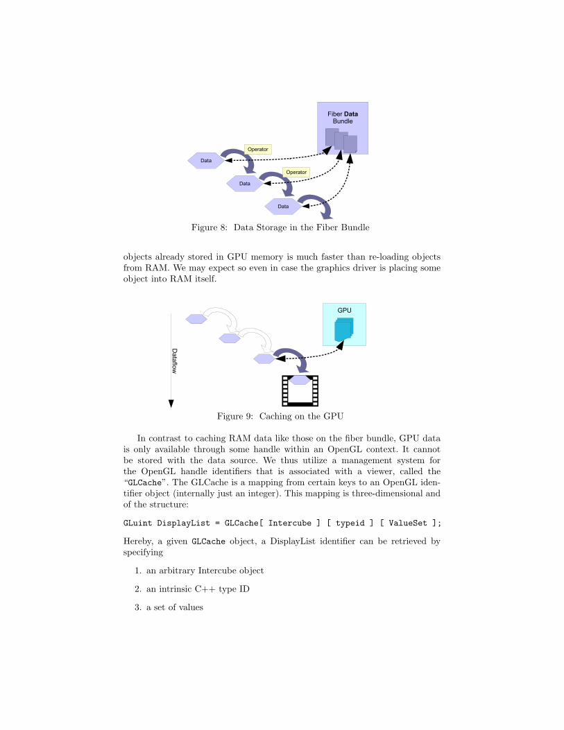
Data
Data
Operator
Data
Operator
Fiber DataBundle
Figure 8: Data Storage in the Fiber Bundle
objects already stored in GPU memory is much faster than re-loading objectsfrom RAM. We may expect so even in case the graphics driver is placing someobject into RAM itself.
Dataflow
GPU
Figure 9: Caching on the GPU
In contrast to caching RAM data like those on the fiber bundle, GPU datais only available through some handle within an OpenGL context. It cannotbe stored with the data source. We thus utilize a management system forthe OpenGL handle identifiers that is associated with a viewer, called the“GLCache”. The GLCache is a mapping from certain keys to an OpenGL iden-tifier object (internally just an integer). This mapping is three-dimensional andof the structure:
GLuint DisplayList = GLCache[ Intercube ] [ typeid ] [ ValueSet ];
Hereby, a given GLCache object, a DisplayList identifier can be retrieved byspecifying
1. an arbitrary Intercube object
2. an intrinsic C++ type ID
3. a set of values
The functionality is similar to the OperatorCache, where an InterCube and avisualization node is utilized to specify a location of the OperatorCache, plusa set of values used to determine whether re-creation of the data is required.Here, the storage location of the cached objects is provided by the GLCache,a parameter that is provided to a visualization object’s render routine. TheInterCube object (which, for instance, is available with each Grid or Field objectwithin a fiber bundle data-set) is used to find a unique storage location withinthe GLCache. The typeid will be the type of the rendering object, such thatmultiple instances of the same rendering functionality will automatically be ableto share their OpenGL objects. The set of values will contain all those renderingparameters which require re-creation of the OpenGL object. A typical renderingcode will (schematically) look like this:
void VizNode::render(GLCache Context, Grid G)ValueSet VS;
// assign cacheable variables into the value setInterCube&C = G;GLuint DisplayList = GLCache[ Intercube ] [ typeid(this) ] [ VS ];if (!DisplayList)
DisplayList = glGenLists(1);glNewList(DisplayList, COMPILE_AND_EXEC);// do actual rendering of grid data GglEndList();GLCache[ Intercube ] [ typeid(this) ] [ VS ] = DisplayList;
else
glCallList(DisplayList);
A similar synopsis will be applied for OpenGL object types others than dis-play lists. Some automatic discarding mechanism to ditch unused objects willbe required here as well. Note that in case an OpenGL object already exists fora given input data-set (here a “Grid” object), then there is no need to actu-ally request the internal data of such an object and to traverse the associatedvisualization pipeline up to its source, such as shown in Figure 10.
3 Conclusion
An universal caching mechanism has been presented. It can be used to extendthe visualization pipeline model (as defined by [Haber & McNabb, 1990]) tomaximize the reuse of computed data and thereby minimizing the responsetime of an interactive visualization to parameter changes. The mechanism canrelate computed data for all parameters of the visualization, which make fastand easy navigation in the whole parameter space possible. Special emphasis
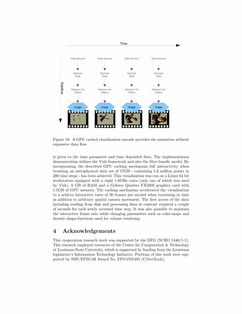
Data Source
Dataflow
DerivedData
Abstract VizObject
Image
Time
Data Source
DerivedData
Abstract VizObject
Image
Data Source
DerivedData
Abstract VizObject
Image
Data Source
DerivedData
Abstract VizObject
Image
Figure 10: A GPU cached visualization cascade provides the animation withoutexpensive data flow.
is given to the time parameter and time depended data. The implementationdemonstration utilizes the Vish framework and also the fiber-bundle model. Byincorporating the described GPU caching mechanism full interactivity whenbrowsing an astrophysical data set of 17GB - containing 1.6 million points in200 time steps - has been achieved. This visualization was run on a Linux 64 bitworkstation equipped with a eight 1.6GHz cores (only one of which was usedby Vish), 8 GB of RAM and a Geforce Quattro FX5600 graphics card with1.5GB of GPU memory. The caching mechanism accelerated the visualizationto a achieve interactive rates of 30 frames per second when traversing in timein addition to arbitrary spatial camera movement. The first access of the dataincluding reading from disk and processing data in contrast required a coupleof seconds for each newly accessed time step. It was also possible to maintainthe interactive frame rate while changing parameters such as color-maps anddensity shape-functions used for volume rendering.
4 Acknowledgements
This cooperation research work was supported by the DFG (SCHO 1346/1-1).This research employed resources of the Center for Computation & Technologyat Louisiana State University, which is supported by funding from the Louisianalegislature’s Information Technology Initiative. Portions of this work were sup-ported by NSF/EPSCoR Award No. EPS-0701491 (CyberTools).

References
[A.A. Ahmed, 2007] A.A. Ahmed, e. a. (2007). Automatic visualization pipelineformation for medical datasets on grid computing environment.
[Benger, 2004] Benger, W. (2004). Visualization of General Relativistic TensorFields via a Fiber Bundle Data Model. PhD thesis, FU Berlin.
[Benger, 2008] Benger, W. (2008). Colliding galaxies, rotating neutron starsand merging black holes - visualising high dimensional data sets on arbi-trary meshes. New Journal of Physics, 10. URL: http://stacks.iop.org/1367-2630/10/125004.
[Benger et al., 2007] Benger, W., Ritter, G., & Heinzl, R. (2007). The conceptsof vish. In 4th High-End Visualization Workshop, Obergurgl, Tyrol, Austria,June 18-21, 2007 (pp. 26–39).: Berlin, Lehmanns Media-LOB.de.
[Benger et al., 2006] Benger, W., Venkataraman, S., Long, A., Allen, G., Beck,S. D., Brodowicz, M., MacLaren, J., & Seidel, E. (2006). Visualizing katrina- merging computer simulations with observations. In Workshop on state-of-the-art in scientific and parallel computing, Umea, Sweden, June 18-21, 2006(pp. 340–350).: Lecture Notes in Computer Science (LNCS), Springer Verlag.
[Bischof et al., 2006] Bischof, H.-P., Dale, E., & Peterson, T. (2006). Spiegel- a visualization framework for large and small scale systems. In MSV (pp.199–205).
[Black et al., 2002] Black, A. P., Huang, J., Koster, R., Walpole, J., & Pu, C.(2002). Infopipes: an abstraction for multimedia streaming. Multimedia Syst.,8(5), 406–419.
[Card et al., 1999] Card, S. K., Mackinlay, J. D., & Shneiderman, B. (1999).Using vision to think. (pp. 579–581).
[Foulser, 1995] Foulser, D. (1995). Iris explorer: a framework for investigation.SIGGRAPH Comput. Graph., 29(2), 13–16.
[Haber & McNabb, 1990] Haber, R. & McNabb, D. A. (1990). Visualization id-ioms: A conceptual model for scientific visualization systems. In Visualizationin Scientific Computing.
[Haeberli, 1988] Haeberli, P. E. (1988). Conman: a visual programming lan-guage for interactive graphics. SIGGRAPH Comput. Graph., 22(4), 103–111.
[Hibbard, 1999] Hibbard, B. (1999). Top ten visualization problems. SIG-GRAPH Comput. Graph., 33(2), 21–22.
[Johnson & Jennings, 2001] Johnson, G. W. & Jennings, R. (2001). LabVIEWGraphical Programming. McGraw-Hill Professional.

[Schroeder et al., 1997] Schroeder, W., Martin, K., & Lorensen, B. (1997). TheVisualization Toolkit: An Object-Oriented Approach to 3D Graphics. PrenticeHall.
[Shen, 2006] Shen, H. (2006). Visualization of large scale time-varying scientificdata. J. of Physics: Conf. Series, 46, 535–544.
[Treinish, 1997] Treinish, L. A. (1997). Data explorer data model. http://www.research.ibm.com/people/l/lloydt/dm/dx/dx_dm.htm.
[Upson et al., 1989] Upson, C., Thomas Faulhaber, J., Kamins, D., Laidlaw, D.,Schlegel, D., Vroom, J., Gurwitz, R., & van Dam, A. (1989). The applicationvisualization system: A computational environment for scientific visualiza-tion. IEEE Computer Graphics and Applications, 9(4), 30–42.

Using Geometric Algebra for Navigation in Riemannianand Hard Disc Space
Werner BengerCenter for Computation &
TechnologyLouisiana State University
239 Johnston HallBaton Rouge, LA 70803, USA
Andrew HamiltonCenter for Astrophysics and
Space AstronomyJILA, University of Colorado
Boulder, CO 80309, [email protected]
Mike Folk/Quincey KoziolThe HDF Group
1901 So. First St. Suite C-2Champaign, IL 61820. USA
Simon SuPrinceton Institute for
Computational Science andEngineering
345 Peter B. Lewis LibraryPrinceton, NJ 08544, USA
Erik SchnetterCenter for Computation &
TechnologyDept. of Physics & Astronomy
Louisiana State UniversityBaton Rouge, LA 70803, USA
Marcel Ritter/Georg RitterDepartment of Computer
ScienceUniversity of InnsbruckTechnikerstrasse 21a
A-6020 Innsbruck, [email protected]
ABSTRACTA “vector” in 3D computer graphics is commonly under-stood as a triplet of three floating point numbers, eventuallyequipped with a set of functions operating on them. Thishides the fact that there are actually different kinds of vec-tors, each of them with different algebraic properties andconsequently different sets of functions. Differential Geome-try (DG) and Geometric Algebra (GA) are the appropriatemathematical theories to describe these different types of“vectors”. They consistently define the proper set of opera-tions attached to each class of “floating point triplet” and al-low to derive what meta-information is required to uniquelyidentify a specific type of vector in addition to its purelynumerical values. We shortly review the various types of“vectors” in 3D computer graphics, their relations to rota-tions and quaternions, and connect these to the terminologyof co-vectors and bi-vectors in DG and GA. Not only in3D, but also in 4D, the elegant formulations of GA yieldto more clarity, which will be demonstrated on behalf ofthe use of bi-quaternions in relativity, allowing for instancea more insightful formulation to determine the Newman-Penrose pseudo scalars from the Weyl tensor.
1. INTRODUCTIONGeometric Algebra and the sometimes mystified conceptof spinors eases implementation and intuition significantly,both in computer graphics and in physics. We demonstratethe concrete application of these concepts in two indepen-dently developed computer graphic software packages, where
Geometric Algebra is used for navigating the camera posi-tion in space and time. Another application example is givenby a simulation code solving Einstein’s equation in gen-eral relativity numerically on supercomputers, outputtingthe Newman-Penrose pseudo scalars as primary quantitiesof interest to study gravitational waves, both for visualiza-tion and observational verification.
Geometric Algebra moreover provides means to describehow the metadata information required per “vector” can beprovided in persistent storage. Given large datasets that areexpensively collected or generated by simulations requiringmillions of CPU hours, it is increasingly important and diffi-cult to be able to share and correctly interpret such datasetsyears after their generation, across different research groupsfrom different fields of science. A unique, standardized,extensible identification of the geometric properties of thedataset elements is a necessary pre-requisite for this. simi-lar to the way in which the IEEE standard for floating pointvalues enables sharing floating point values. We utilize themechanisms as provided by the HDF5 library here, a genericself-describing file format developed for large datasets asused in high performance computing. It allows specifyingmetadata in addition to the purely numerical data, providingan abstraction layer for specifying the mathematical prop-erties on top of the lower-level binary layout. It is thereforedesirable to us the functionality of this powerful I/O libraryto express the semantics of vector quantities as they arise inGeometric Algebra. This will be discussed in section 5.
2. VECTOR SPACESA vector space over a field F (such as R) is a set V togetherwith two binary operations vector addition + : V × V → Vand scalar multiplication : F × V → V . The elementsof V are called vectors. A vector space is closed under theoperations + and , i.e., for all elements u, v ∈ V and all el-ements λ ∈ F there is u+v ∈ V and λu ∈ V (vector spaceaxioms). The vector space axioms allow computing the dif-

ferences of vectors and therefore defining the derivative of avector-valued function v(s) : R→ V as
d
dsv(s) := lim
ds→0
v(s+ ds)− v(s)
ds. (1)
2.1 Tangential VectorsIn differential geometry, a tangential vector on a manifoldM is the operator d
dsthat computes the derivative along a
curve q(s) : R → M for an arbitrary scalar-valued functionf : M → R:
d
dsf
∣∣∣∣q(s)
:=df (q(s))
ds. (2)
Tangential vectors fulfill the vector space axioms and cantherefore be expressed as linear combinations of deriva-tives along the n coordinate functions xµ : M → R withµ = 0 . . . n− 1, which define a basis of the tangential spaceTq(s)(M) on the n-dimensional manifold M at each pointq(s) ∈M :
d
dsf =
n−1∑µ=1
dxµ (q(s))
ds
∂
∂xµf =:
n−1∑µ=1
qµ∂µf (3)
where qµ are the components of the tangential vector dds
inthe chart xµ and ∂µ are the basis vectors of the tangen-tial space in this chart. We will use the Einstein sum conven-tion in the following text, which assumes implicit summationover indices occurring on the same side of an equation. Of-ten tangential vectors are used synonymous with the term“vectors” in computer graphics when a direction vector frompoint A to point B is meant. A tangential vector on ann-dimensional manifold is represented by n numbers in achart.
2.2 Co-VectorsThe set of operations df : T (M) → R that map tangentialvectors v ∈ T (M) to a scalar value v(f) for any functionf : M → R defines another vector space which is dual to thetangential vectors. Its elements are called co-vectors.
< df, v >= df(v) := v(f) = vµ∂µf = vµ∂f
∂xµ(4)
Co-vectors fulfill the vector space axioms and can be writtenas linear combination of co-vector basis functions dxµ:
df =:∂f
∂xµdxµ (5)
with the dual basis vectors fulfilling the duality relation
< dxν , ∂µ >=
µ = ν : 1
µ 6= ν : 0(6)
The space of co-vectors is called the co-tangential spaceT ∗p (M). A co-vector on an n-dimensional manifold is repre-sented by n numbers in a chart, same as a tangential vector.However, co-vector transforms inverse to tangential vectorswhen changing coordinate systems, as is directly obviousfrom eq. (6) in the one-dimensional case: As < dx0, ∂0 >= 1must be sustained under coordinate transformation, dx0
must shrink by the same amount as ∂0 grows when an-other coordinate scale is used to represent these vectors.In higher dimensions this is expressed by an inverse trans-formation matrix, as demonstrated in Fig. 1. In Euclidean
Figure 1: Vector transformation under shrinking theheight coordinate by a factor of two: tangential vec-tors (differences between two points) shrink in theirheight component by a factor two as well, whereassurface normal vectors (co-vectors) grow by a fac-tor two in height, see the vertical components of thevector and co-vector shown on the right hand sidein the figure.
three-dimensional space, a plane is equivalently described bya “normal vector”, which is orthogonal to the plane. While“normal vectors” are frequently symbolized via a vector ar-row, like tangential vectors, they are not the same, ratherthey are dual to tangential vectors. It is more appropri-ate to visually symbolize them as a plane. This visual isalso supported by (5), which can be interpreted as the to-tal differential of a function f : a co-vector describes how ascalar function advances in space, which can be visualizedas surfaces of constant function value (“isosurface”). On ann-dimensional manifold a co-vector is correspondingly sym-bolized by an (n− 1)-dimensional subspace.
2.3 TensorsA tensor Tnm of rank n×m is a multi-linear map of n vectorsand m co-vectors to a scalar
Tnm : T (M)× ...T (M)︸ ︷︷ ︸n
×T ∗(M)× ...T ∗(M)︸ ︷︷ ︸m
→ R . (7)
Tensors are elements of a vector space themselves and formthe tensor algebra. They are represented relative to a coor-dinate system by a set of kn+m numbers for a k-dimensionalmanifold. The construction of an tensor of higher rank fromlower rank is called the outer product (or tensor product),denoted by ⊗:
T ≡ T ab∂a ⊗ ∂b = vaub∂a ⊗ ∂b = va∂a ⊗ ub∂b = v ⊗ u (8)
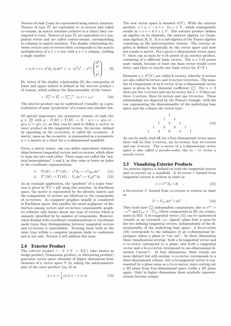
Tensors of rank 2 may be represented using matrix notation.Tensors of type T 0
1 are equivalent to co-vectors and calledco-variant, in matrix notation (relative to a chart) they cor-respond to rows. Tensors of type T 1
0 are equivalent to a tan-gential vector and are called contra-variant, correspondingto columns in matrix notation. The duality relationship be-tween vectors and co-vectors then corresponds to the matrixmultiplication of a 1× n row with a n× 1 column, yieldinga single number
< a, b >=< aµ∂µ, bµdxµ > ≡ (a0a1 . . . an)
b0
b1
. . .bn
. (9)
By virtue of the duality relationship (6) the contraction oflower and upper indices is defined as the interior product ιof tensors, which reduces the dimensionality of the tensor:
ι : Tmn × T lk → Tm−kn−l : u, v 7→ ιuv (10)
The interior product can be understood (visually) as a gen-eralization of some“projection”of a tensor onto another one.
Of special importance are symmetric tensors of rank twog ∈ T 0
2 with g : T (M) × T (M) → R : u, v 7→ g(u, v) ,g(u, v) = g(v, u), as they can be used to define a metric orinner product on the tangential vectors. Its inverse, definedby operating on the co-vectors, is called the co-metric. Ametric, same as the co-metric, is represented as a symmetricn× n matrix in a chart for a n-dimensional manifold.
Given a metric tensor, one can define equivalence relation-ships between tangential vectors and co-vectors, which allowto map one into each other. These maps are called the “mu-sical isomorphisms”, [ and ], as they raise or lower an indexin the coordinate representation:
[ : T (M)→ T ∗(M) : vµ∂µ 7→ vµgµνdxν (11)
] : T ∗(M)→ T (M) : Vµdxµ 7→ Vµg
µν∂ν (12)
As an example application, the “gradient” of a scalar func-tion is given by ∇f = ]df using this notation. In Euclideanspace, the metric is represented by the identity matrix andthe components of vectors are identical to the componentsof co-vectors. As computer graphics usually is consideredin Euclidean space, this justifies the usual negligence of dis-tinction among vectors and co-vectors; consequently graph-ics software only knows about one type of vectors which isuniquely identified by its number of components. However,when dealing with coordinate transformations or curvilinearmesh types then distinguishing between tangential vectorsand co-vectors is unavoidable. Treating them both as thesame type within a computer program leads to confusionsand is not safe. Section 4 will address this issue.
2.4 Exterior ProductThe exterior product ∧ : V × V → Λ(V ) (also known aswedge product, Grassmann product, or alternating product)generates vector space elements of higher dimensions fromelements of a vector space V by taking the antisymmetricpart of the outer product (eq. 8) as
u ∧ v =1
2(u⊗ v − v ⊗ u) (13)
The new vector space is denoted Λ(V ). With the exteriorproduct, v ∧ u = −u ∧ v ∀u, v ∈ V , which consequentlyresults in v ∧ v = 0 ∀ v ∈ V . The exterior product definesan algebra on its elements, the exterior algebra (or Grass-man algebra) [9, 5]. It is a sub-algebra of the Tensor algebraconsisting on the anti-symmetric tensors. The exterior al-gebra is defined intrinsically by the vector space and doesnot require a metric. For a given n-dimensional vector spaceV , there can at most be n-th power of an exterior product,consisting of n different basis vectors. The n + 1-th powermust vanish, because at least one basis vector would occurtwice, and there is exactly one basis vector for Λn(V ).
Elements v ∈ Λk(V ) are called k-vectors, whereby 2-vectorsare also called bi-vectors and 3-vectors trivectors. The num-ber of components of an k-vector of an n-dimensional vectorspace is given by the binomial coefficient
(nk
). For n = 2
there are two 1-vectors and one bi-vector, for n = 3 there arethree 1-vectors, three bi-vectors and one tri-vector. Theserelationships are depicted by the Pascal’s triangle, with therow representing the dimensionality of the underlying basespace and the column the vector type:
11 1
1 2 11 3 3 1
1 4 6 4 1
(14)
As can be easily read off, for a four-dimensional vector spacethere will be four 1-vectors, six bi-vectors, four tri-vectorsand one 4-vector. The n-vector of a n-dimensional vectorspace is also called a pseudo-scalar, the (n − 1) vector apseudo-vector.
2.5 Visualizing Exterior ProductsAn exterior algebra is defined on both the tangential vectorsand co-vectors on a manifold. A bi-vector v formed fromtangential vectors is written in chart as
v = vµν∂µ ∧ ∂ν , (15)
a bi-covector U formed from co-vectors is written in chartas
U = Uµνdxµ ∧ dxν . (16)
They both have(n2
)independent components, due to vµν =
−vνµ and Uµν = −Uνµ (three components in 3D, six compo-nents in 4D). A bi-tangential vector (15) can be understoodvisually as an (oriented, i.e., signed) plane that is spun bythe two defining tangential vectors, independently of the di-mensionality of the underlying base space. A bi-co-vector(16) corresponds to the subspace of an n-dimensional hy-perspace where a plane is “cut out”. In three dimensionsthese visualizations overlap: both a bi-tangential vector anda co-vector correspond to a plane, and both a tangentialvector and a bi-co-vector correspond to one-dimensional di-rection (“arrow”). In four dimensions, these visuals aremore distinct but still overlap: a co-vector corresponds to athree-dimensional volume, but a bi-tangential vector is rep-resented by a plane same as a bi-co-vector, since cutting outa 2D plane from four-dimensional space yields a 2D planeagain. Only in higher dimensions these symbolic represen-tations become unique.

1
1 1
1 2 1
1 3 3 1
1 4 6 4 1
1 5 10 10 5 1
Tangential Vectors∂x
Co-Vectors /Pseudo-Vectors
dxBi-Co-Vectors dx^dy Bi-Vectors
∂x ^ ∂y
0D
1D
2D
3D
4D
5D
Figure 2: Pascal’s triangle showing the locationof tangential vectors, bi-vectors, co-vectors and bi-covectors in the various subspaces in different di-mensions. Especially in three dimensions there aremany overlaps, indicating ambiguities where differ-ent quantities are all represented by “just threenumbers”. Similar situations occur in 4D, only in5D all vector types become unambiguous.
However, in any case a co-vector and a pseudo-vector willhave the same appearance as an n − 1 dimensional hyper-space, same as a tangential vector corresponds to an pseudo-co-vector:
Vµdxµ ⇔ vα0α1...αn−1 ∂α0 ∧ ∂α1 ∧ . . . ∂αn−1 (17)
vµ∂µ ⇔ Vα0α1...αn−1 dxα0 ∧ dxα1 ∧ . . . dxαn−1 (18)
A tangential vector – lhs of (18) – can be understood asone specific direction, but equivalently as well as “cuttingoff” all but one n − 1-dimensional hyperspaces from an n-dimensional hyperspace – rhs of (18). This equivalence isexpressed via the interior product of a tangential vector vwith an pseudo-co-scalar Ω yielding a pseudo-co-vector V(19), similarly the interior product of a pseudo-vector withan pseudo-co-scalar yielding a tangential vector (19):
ιΩ : T (M) → (T ∗)(n−1)(M) : V 7→ ιΩv (19)
ιΩ : T (n−1)(M) → T ∗(M) : V 7→ ιΩv (20)
Pseudo-scalars and pseudo-co-scalars will always be scalarmultiples of the basis vectors ∂α0 ∧ ∂α1 ∧ . . . ∂αn anddxα0 ∧ dxα1 ∧ . . . dxαn . However, under when inversing acoordinate xµ → −xµ they flip sign, whereas a “true” scalardoes not. An example known from Euclidean vector algebrais the allegedly scalar value constructed from the dot andcross product of three vectors V (u, v, w) = u· (v×w) whichis the negative of when its arguments are flipped:
V (u, v, w) = −V (−u,−v,−w) = −u· (−v ×−w) . (21)
which is actually more obvious when (21) is written as ex-terior product:
V (u, v, w) = u ∧ v ∧ w = V ∂0 ∧ ∂1 ∧ ∂2 (22)
The result (22) actually describes a multiple of a volumeelement span by the basis tangential vectors ∂µ - any vol-ume must be a scalar multiple of this basis volume element,
but can flip sign if another convention on the basis vec-tors is used. This convention depends on the choice of aright-handed versus left-handed coordinate system, and isexpressed by the orientation tensor Ω = ±∂0 ∧ ∂1 ∧ ∂2. Incomputer graphics, both left-handed and right-handed co-ordinate systems occur, which often causes confusion.
By combining (20) and (12) – requiring a metric – we get amap from pseudo-vectors to vectors and reverse. This mapis known as the Hodge star operator “∗”:
∗ : T (n−1)(M)→ T (M) : V 7−→ ]ιΩV (23)
The same operation can be applied to the co-vectors accord-ingly, and generalized to all vector elements of the exterioralgebra on a vector space, establishing a correspondence be-tween k−vectors and n−k-vectors. The Hodge star operatorallows to identify vectors and pseudo-vectors, similarly tohow a metric allows to identify vectors and co-vectors. TheHodge star operator requires a metric and an orientation Ω.
A prominent application in physics using the hodge star op-erator are the Maxwell equations, which, when written basedon the four-dimensional potential A = V0dx
0 + Akdxk (V0
the electrostatic, Ak the magnetic vector potential) take theform
d ∗ dA = J (24)
with J the electric current and magnetic flow, which is zeroin vacuum. The combination d ∗ d is equivalent to theLaplace operator “2”, which indicates that (24) describeselectromagnetic waves in vacuum.
2.6 Geometric AlgebraGeometric Algebra is motivated by the intention to find aclosed algebra on a vector space with respect to multiplica-tion, which includes existence of an inverse operation. Thereis no concept of dividing vectors in “standard” vector alge-bra. Because the result of the inner and exterior product isof different dimensionality than their operands, they are notsuited to define a closed GA on the vector space.
Geometric algebra postulates a product on elements of avector space u, v, w ∈ V that is associative, (uv)w = u(vw),left-distributive u(v+w) = uv+ uw, right-distributive (u+v)w = uw+vw, and reduces to the inner product as definedby the metric v2 = g(v, v). It can be shown that sum ofthe exterior product (which, within Geometric Algebra, isalso called outer product, but should not be confused withthe outer product ⊗ on tensors from eq. 8) and the innerproduct fulfill these requirements; this defines the geometricproduct as the sum of both:
uv := u ∧ v + u · v . (25)
Since u ∧ v and u · v are of different dimensionality ((n2
)and
(n0
), respectively), the result must be in a higher dimen-
sional vector space of dimensionality(n2
)+(n0
). This space is
formed by the linear combination of k-vectors, its elementsare called multivectors. Its dimensionality is
∑n−1k=0
(nk
)≡ 2n.
For instance, in two dimensions the dimension of the spaceof multivectors is 22 = 4. A multivector V , constructed fromtangential-vectors on a two-dimensional manifold, is written

Figure 3: Graphical representation of the 1+3+3+1structure of components that build a 3D multivec-tor: three tangential vectors, three oriented planes,one scalar and one (oriented) volume element.
as
V = V 0 + V 1∂0 + V 2∂1 + V 3∂0 ∧ ∂1 (26)
with V µ the four components of the multivector in a chart.For a three-dimensional manifold a multivector on its tan-gential space has 23 = 8 components and is written as
V =V 0+
V 1∂0 + V 2∂1 + V 2∂2+
V 4∂0 ∧ ∂1 + V 5∂1 ∧ ∂2 + V 6∂2 ∧ ∂0+
V 7∂0 ∧ ∂1 ∧ ∂2
(27)
with V µ the eight components of the multivector in a chart.The components of a multivector have a direct visual in-terpretation, which is one of the key features of geometricalgebra. In 3D, a multivector is the sum of a scalar value,three directions, three planes and one volume. These basiselements span the entire space of multivectors.
2.7 Spinors and QuaternionsGiven a bi-vector U = u∧v built from two orthonormal unitvectors u, v (which fulfill |u| = 1, |v| = 1, u · v = 0 under agiven metric such that U = uv), we find that it provides thesame algebraic properties as the imaginary unit
√−1:
U2 = UU = (uv)(uv) = (uv)(−vu) = −u(vv)u = −1 (28)
This is a well known aspect of Geometric Algebra, whichleads to n distinct imaginary units on an n-dimensional vec-tor space. For n = 3 we have three imaginary units (usu-ally denoted as i, j, k), which relate to the three bi-vectorsalong the three coordinate axis. These three basis vectorsi = ∂x∧∂y, j = ∂y ∧∂z, k = ∂z ∧∂x (equivalently to the co-vectors) fulfill ijk = −1, which is identical to the definitionsused in Quaternion algebra [7]. A quaternion consists of fourcomponents, a scalar and “vectorial” part. They represent
the even parts of a multivector in 3D (27):
Q = Q0 +Q2∂0 ∧ ∂1 +Q0∂1 ∧ ∂2 +Q1∂2 ∧ ∂0 (29)
It can be shown that the even multivectors form a closed sub-algebra itself. GA provides a direct geometric insight forquaternions via (29), with the hard-to-memorable quater-nion product being immersed within the easily remember-able geometric product. Given an even multivector (29), itsdual as provided by the Hodge star operator (23) yields anodd multivector, consisting out of a tangential vector and apseudo-scalar (i.e., a volume element).
Quaternions are known in computer graphics for implement-ing rotations (for instance, the SbRotation class in OpenIn-ventor), alternatively to rotation matrices (such as used inOpenGL). Same functionality is provided by rotors in GA.In 2D the right-multiplication of a vector v = vx∂x + vy∂ywith the bi-vector ∂x ∧ ∂y = ∂x∂y corresponds to a counter-clockwise rotation:
v(∂x ∧ ∂y) = vx∂x(∂x∂y) + vy∂y(∂x∂y) = vx∂y − vy∂x (30)
Therefore a rotation around an arbitrary angle ϕ is writtenas a linear combination of a scalar component and a bi-vector, which is called a rotor (or spinor):
R = cosϕ+ i sinϕ =: ei (31)
where i is an arbitrary unit bi-vector fulfilling i2 = −1.e is the Euler number used here for defining the exponen-tial function of a bi-vector, in style of the Euler equation.The inverse rotor (implementing clockwise rotation on right-multiplication, or counter-clockwise when applied from theleft) is given by inversing the rotation angle
R−1 = e−i = cosϕ− i sinϕ . (32)
In two dimensions it is equivalent if some vector v is left-multiplied or right-multiplied with a rotor
vR−2 ≡ R2v ≡ RvR−1 , (33)
however in more than two dimensions the symmetric variantRvR−1 with multiplying from the left and from the righthas to be used to cancel out a tri-vector component thatwould otherwise occur (from multiplying the vector with athe bi-vector part of the rotor). While Quaternion Algebrais specific to three dimensions, the concept of a rotor in GAis independent from the dimensions and directly applicableto the 4D case, as will be reviewed in the next section.
2.8 Multilinear Multivector MapsSame as a tensor is a multilinear map of vectors and co-vectors, we may represent multilinear maps of multivectorsas a set of numbers given a specific chart. The Riemanntensor R, as described in 3.3, is such a case, is it can be seenas a map from bivectors to bivectors:
R : Tp(M) ∧ Tp(M)→ Tp(M) ∧ Tp(M) (34)
The Riemann tensor can then be interpreted as argument ofthe Lorentz boost eR(U) resulting from a tiny circuit withina plane defined by the bivector U .
3. NEWMAN-PENROSE FORMALISMGeneral relativity predicts the existence of gravitationalwaves. There is a huge effort to detect gravitational waves

Figure 4: The two linear polarizations of gravita-tional waves. The + polarization (top) has a cos 2χshape about the direction of propagation (into thepaper), while the × polarization (bottom) has asin 2χ shape. A gravitational wave causes a systemof freely falling test masses to oscillate relative to agrid of points a fixed proper distance apart.
expected for example from merging pairs of black holes [1].To date no gravitational waves have been detected directly.There is however indirect evidence for their existence fromthe gradual decrease in orbital period of the binary pulsar,which is quantitatively consistent with the general relativis-tic prediction of energy loss by quadrupole emission of grav-itational waves [4, 6].
It is conventional to characterize gravitational waves interms of their Newman-Penrose (1962) (NP) components[14, 2, 16]. The purpose of this section is to give an ideaof how this works, and how the geometric algebra offers in-sight into the NP formalism. The traditional derivation ofthe NP components of gravitational waves is magical, andshrouded in unnecessary and misleading notation. As Held(1974) [13] politely puts it, the NP formalism presents “aformidable notational barrier to the uninitiate”.
The notion of a gravitational wave can be perplexing. Apassing gravitational wave causes the distance between twofreeling-falling masses to oscillate. But if gravity affects thevery measurement of length itself, how can the distance be-tween the masses be measured? The answer is that, despitethe fact that in general relativity spacetime has no absoluteexistence, in the sense that the choice of coordinate system
is arbitrary, nevertheless the metric asserts that there is aunique proper distance along a given path (or affine distance,along a null path) between any two points in spacetime (suchas the path followed by a beam of laser light). The presenceof gravity, or curvature, is expressed by the presence of agravitational force between two points a fixed proper dis-tance apart. A gravitational wave causes an oscillation inthe differential gravitational force, or tidal force, betweentwo points a fixed distance apart.
Figure 4 illustrates gravitational waves, in their two possi-ble linear polarizations, + and ×. The grid represents a lo-cally inertial system of points a fixed proper distance apart.The superposed ellipses represent a system of freely-fallingtest masses whose positions, initially on a circle, are be-ing perturbed by a gravitational wave moving in a directionperpendicular to the paper. The proper distance betweenfreely-falling test masses oscillates. That oscillation can bemeasured for example by the change in the number of wave-lengths along a laser beam between the masses.
Sometimes one sees depictions of gravitational waves simi-lar to Figure 4, but with the grid oscillating along with theellipses. Such depictions are intended to convey the ideathat gravitational waves are waves of spacetime (of the met-ric), but they are misleading, since they suggest that rulersoscillate along with the test masses, which is false.
3.1 Newman-Penrose tetradThe Newman-Penrose (NP) formalism is particularly welladapted to treating waves that travel at the speed of light,which includes electromagnetic and gravitational waves.The NP formalism starts with the rest frame of an observer,and applies two tricks to it. The axes, or tetrad, of the ob-server’s locally inertial frame form an orthonormal basis ofvectors in the geometric algebra
γt,γx,γy,γz , (35)
with the metric in Minkowski signature of the form
γm · γn =
−1 0 0 00 1 0 00 0 1 00 0 0 1
(36)
with indices m, n running over t, x, y, z. The NP formalismchooses one axis, typically the z-axis, to be the direction ofpropagation of the wave.
The first NP trick is to replace the transverse axes γx andγy by spinor axes γ+ and γ− defined by
γ+ ≡1√2
(γx + Iγy) , γ− ≡1√2
(γx − Iγy) . (37)
This is the same trick used to define the spinor componentsL± of the angular momentum operator L in quantum me-chanics.
The second NP trick is to replace the time t and propaga-tion z axes with outgoing and ingoing null axes γv and γu,defined by
γv ≡1√2
(γt + γz) , γu ≡1√2
(γt − γz) . (38)

The resulting outgoing, ingoing, and spinor axes form a NPnull tetrad
γv,γu,γ+,γ− , (39)
with NP metric
γm · γn =
0 −1 0 0−1 0 0 00 0 0 10 0 1 0
(40)
with indices m, n running over v, u,+,−. The NP met-ric (40) has zeros down the diagonal. This means that eachof the four NP axes γm is null: the scalar product of eachaxis with itself is zero. In a profound sense, the null, or light-like, character of each the four NP axes explains why the NPformalism is well adapted to treating fields that propagateat the speed of light.
Three kinds of transformation, considered further below,take a particularly simple form in the NP tetrad:
I Reflections through the transverse axis y;II Rotations about the propagation axis z;
III Boosts along the propagation axis z.
3.1.1 ReflectionsUnder transformation I, a reflection through the y-axis, thespinor axes swap:
γ+ ↔ γ− , (41)
which may also be accomplished by complex conjugation.Reflection through the y-axis, or equivalently complex con-jugation, changes the sign of all spinor indices of a tensorcomponent
+↔ − . (42)
In short, complex conjugation flips spin, a pretty feature ofthe NP formalism.
3.1.2 RotationsUnder transformation II, a right-handed rotation by angleχ about the direction z of propagation, the transverse axesγx and γy transform as
γx → cosχ γx − sinχ γy ,
γy → sinχ γx + cosχ γy . (43)
It follows that the spinor axes γ+ and γ− transform undera right-handed rotation by angle χ as
γ± → e±Iχ γ± . (44)
The transformation (44) identifies the spinor axes γ+ andγ− as having spin +1 and −1 respectively. More generally,an object can be defined as having spin s if it varies by
esIχ (45)
under a rotation by angle χ about the direction of propaga-tion. The NP components of a tensor inherit spin propertiesfrom that of the spinor basis. The general rule is that thespin s of any tensor component is equal to the number of +covariant indices minus the number of − covariant indices:
spin s = number of + minus − covariant indices . (46)
3.1.3 BoostsThe final transformation III, a boost along the z-axis, multi-plies the outgoing and ingoing axes γv and γu by a blueshiftfactor ε and its reciprocal
γv → εγv ,
γu → (1/ε)γu . (47)
If the observer boosts by velocity v in the z-direction awayfrom the source, then the blueshift factor is the special rel-ativistic Doppler shift factor
ε =
(1− v1 + v
)1/2
. (48)
The exponent n of the power εn by which an object changesunder a boost along the z-axis is called its boost weight.Thus γv has boost weight +1, and γu has boost weight −1.The NP components of a tensor inherit their boost weightproperties from those of the NP basis. The general rule isthat the boost weight n of any tensor component is equalto the number of v covariant indices minus the number of ucovariant indices:
boost weight n = number of v minus u covariant indices .(49)
3.2 Electromagnetic wavesThe properties of gravitational waves are in many ways sim-ilar to those of electromagnetic waves. Both kinds of wavesare massless, traveling at the speed of light. A crucial dif-ference is that gravitational waves are spin-2 (tensor) waves,whereas electromagnetic waves are spin-1 (vector) waves.
Recall the nature of electromagnetic waves. Electromag-netic waves are characterized by the electromagnetic fieldFij , which is an antisymmetric tensor, or bivector, with 6distinct components. The 6 components are commonly col-lected into two 3-dimensional vectors, the electric and mag-netic fields E and B. The geometric algebra gives the insightthat the electromagnetic field tensor, being a bivector, hasa natural complex structure, in which the electric and mag-netic fields together form a complex 3-vector E + IB.
With respect to a NP null tetrad (39), the electromagneticbivector has 3 complex components, of spin respectively −1,0, and +1, in accordance with the rule (46):
− 1 : Fu−
0 :1
2(Fuv + F+−)
+1 : Fv+ . (50)
The complex conjugates of the 3 components are:
− 1∗ : Fu+
0∗ :1
2(Fuv − F+−)
+1∗ : Fv− , (51)
whose spins have the opposite sign. Conventionally (Chan-drasekhar 1983), the 3 complex spin components of the elec-

tromagnetic field bivector in the NP formalism are denoted
− 1 : φ2 ,
0 : φ1 ,
+1 : φ0 . (52)
The notation, like much of the rest of conventional NP no-tation, is truly awful.
For outgoing electromagnetic waves, only the spin −1component propagates, carrying electromagnetic energy faraway from a source:
− 1 : propagating, outgoing . (53)
This propagating, outgoing −1 component has spin −1, butits complex conjugate has spin +1, so effectively both spincomponents, or helicities, of an outgoing wave are embodiedin the single complex component. The remaining 2 complexNP components (spins 0 and 1) of an outgoing wave areshort range, describing the electromagnetic field near thesource.
Similarly, for ingoing waves, only the spin +1 componentpropagates.
The isolation of each propagating mode into a single com-plex NP mode, incorporating both helicities, is simpler thanthe standard picture of oscillating orthogonal electric andmagnetic fields.
3.3 Gravitational wavesIn electromagnetism, the electromagnetic field tensor is de-fined by the commutator of the gauge-covariant derivative.In general relativity, the analogous commutator of the co-variant derivative is the Riemann curvature tensor Rklmn.The Riemann curvature tensor has symmetries which can bedesignated shorthandly
R([kl][mn]) . (54)
Here [] denotes antisymmetry, and () symmetry. The desig-nation (54) thus signifies that the Riemann curvature tensorRklmn is antisymmetric in its first two indices kl, antisym-metric in its last two indices mn, and symmetric under ex-change of the first and last pairs of indices, kl ↔ mn. Inaddition to the symmetries (54), the Riemann curvature ten-sor has the totally antisymmetric symmetry
Rklmn +Rkmnl +Rknlm = 0 . (55)
The symmetries (54) imply that that the Riemann curva-ture tensor is a symmetric matrix of antisymmetric tensors,which is to say, a 6 × 6 symmetric matrix of bivectors. A6×6 symmetric matrix has 21 independent components. Theadditional condition (55) eliminates one degree of freedom,leaving the Riemann curvature tensor with 20 independentcomponents.
In spacetime algebra any bivector U (6 component) can bewritten as complex sum U = (E + IB)γt of two spatial 3-vectors E = Exγx +Eyγy +Bzγz and B = Bxγx +Byγy +Bzγz, due to the identity Iγxγt ≡ γyγz etc. In analogy toelectromagnetism, Eγt is called the electric bivector, Bγtthe magnetic bivector. The Riemann tensor, a multilinear
multimap on bivectors eq. (34), can then be organized intoa 2× 2 matrix of 3× 3 blocks with bivector indices, yieldingthe structure (
REE REBRBE RBB
). (56)
The condition of being symmetric implies that REE andRBB are symmetric, while RBE = (REB)>. The condi-tion (55) states that the 3×3 block REB (and likewise RBE)is traceless.
The natural complex structure of bivectors in the geomet-ric algebra suggests recasting the 6 × 6 Riemann curvaturematrix (56) into a 3× 3 complex matrix, which would havethe structure (RE + IRB)(RE + IRB), or equivalently
REE −RBB + I(REB +RBE) , (57)
which is a complex linear combination of the four 3×3 blocksof the Riemann matrix (56). However, it turns out that thecomplex symmetric 3×3 matrix (57) encodes only part of theRiemann curvature tensor, namely the Weyl tensor. Morespecifically, the Riemann curvature tensor decomposes intoa trace part, the Ricci tensor Rkm, and a totally tracelesspart, the Weyl tensor Cklmn. The Ricci tensor, which is sym-metric, has 10 independent components. The Weyl tensor,which inherits the symmetries (54) and (55) of the Riemantensor, and in addition vanishes on contraction of any pairof indices, also has 10 independent components. Together,the Ricci and Weyl tensors account for the 20 componentsof the Riemann tensor. The components of the Ricci andWeyl tensors, though algebraically independent, are relatedby the differential Bianchi identities.
The end result is that the Weyl tensor, the traceless partof the Riemann curvature tensor, can be written as a 3× 3complex traceless symmetric matrix (57). Such a matrix has5 distinct complex components.
In empty space (vanishing energy-momentum tensor), theRicci tensor vanishes identically. Thus the properties of thegravitational field in empty space are specified entirely bythe Weyl tensor. In particular, gravitational waves are spec-ified entirely by the Weyl tensor.
When the 5 complex components of the Weyl tensor areexpressed in a NP null tetrad (39), the result is 5 complexcomponents, of spins respectively −2, −1, 0, +1, and +2:
− 2 : Cu−u−
−1 : Cuvu−
0 :1
2(Cvuvu + Cvu−+)
+1 : Cvuv+ (58)
+2 : Cv+v+ . (59)
It can be shown that these 5 complex components exhaustthe degrees of freedom of the Weyl tensor.
For outgoing gravitational waves, only the spin −2 com-ponent propagates, carrying gravitational waves to far dis-tances:
− 2 : propagating, outgoing . (60)
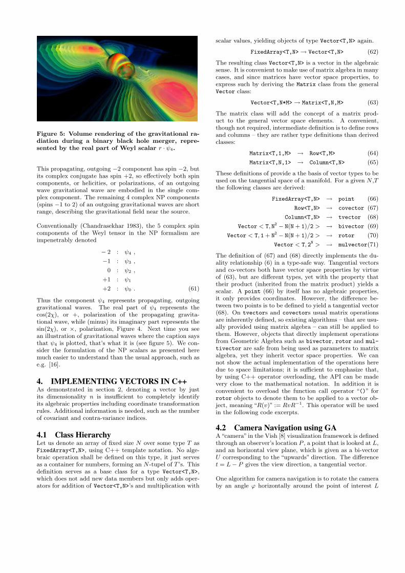
Figure 5: Volume rendering of the gravitational ra-diation during a binary black hole merger, repre-sented by the real part of Weyl scalar r · ψ4.
This propagating, outgoing −2 component has spin −2, butits complex conjugate has spin +2, so effectively both spincomponents, or helicities, or polarizations, of an outgoingwave gravitational wave are embodied in the single com-plex component. The remaining 4 complex NP components(spins −1 to 2) of an outgoing gravitational waves are shortrange, describing the gravitational field near the source.
Conventionally (Chandrasekhar 1983), the 5 complex spincomponents of the Weyl tensor in the NP formalism areimpenetrably denoted
− 2 : ψ4 ,
−1 : ψ3 ,
0 : ψ2 ,
+1 : ψ1
+2 : ψ0 . (61)
Thus the component ψ4 represents propagating, outgoinggravitational waves. The real part of ψ4 represents thecos(2χ), or +, polarization of the propagating gravita-tional wave, while (minus) its imaginary part represents thesin(2χ), or ×, polarization, Figure 4. Next time you seean illustration of gravitational waves where the caption saysthat ψ4 is plotted, that’s what it is (see figure 5). We con-sider the formulation of the NP scalars as presented heremuch easier to understand than the usual approach, such ase.g. [16].
4. IMPLEMENTING VECTORS IN C++As demonstrated in section 2, denoting a vector by justits dimensionality n is insufficient to completely identifyits algebraic properties including coordinate transformationrules. Additional information is needed, such as the numberof covariant and contra-variance indices.
4.1 Class HierarchyLet us denote an array of fixed size N over some type T asFixedArray<T,N>, using C++ template notation. No alge-braic operation shall be defined on this type, it just servesas a container for numbers, forming an N -tupel of T ’s. Thisdefinition serves as a base class for a type Vector<T,N>,which does not add new data members but only adds oper-ators for addition of Vector<T,N>’s and multiplication with
scalar values, yielding objects of type Vector<T,N> again.
FixedArray<T,N>→ Vector<T,N> (62)
The resulting class Vector<T,N> is a vector in the algebraicsense. It is convenient to make use of matrix algebra in manycases, and since matrices have vector space properties, toexpress such by deriving the Matrix class from the generalVector class:
Vector<T,N*M>→ Matrix<T,N,M> (63)
The matrix class will add the concept of a matrix prod-uct to the general vector space elements. A convenient,though not required, intermediate definition is to define rowsand columns – they are rather type definitions than derivedclasses:
Matrix<T,1,M> → Row<T,M> (64)
Matrix<T,N,1> → Column<T,N> (65)
These definitions of provide a the basis of vector types to beused on the tangential space of a manifold. For a given N ,Tthe following classes are derived:
FixedArray<T,N> → point (66)
Row<T,N> → covector (67)
Column<T,N> → tvector (68)
Vector < T, N2 − N(N + 1)/2 > → bivector (69)
Vector < T, 1 + N2 − N(N + 1)/2 > → rotor (70)
Vector < T, 2N > → mulvector(71)
The definition of (67) and (68) directly implements the du-ality relationship (6) in a type-safe way. Tangential vectorsand co-vectors both have vector space properties by virtueof (63), but are different types, yet with the property thattheir product (inherited from the matrix product) yields ascalar. A point (66) by itself has no algebraic properties,it only provides coordinates. However, the difference be-tween two points is to be defined to yield a tangential vector(68). On tvectors and covectors usual matrix operationsare inherently defined, so existing algorithms – that are usu-ally provided using matrix algebra – can still be applied tothem. However, objects that directly implement operationsfrom Geometric Algebra such as bivector, rotor and mul-
tivector are safe from being used as parameters to matrixalgebra, yet they inherit vector space properties. We cannot show the actual implementation of the operations heredue to space limitations; it is sufficient to emphasize that,by using C++ operator overloading, the API can be madevery close to the mathematical notation. In addition it isconvenient to overload the function call operator “()” forrotor objects to denote them to be applied to a vector ob-ject, meaning “R(v)” := RvR−1. This operator will be usedin the following code excerpts.
4.2 Camera Navigation using GAA“camera” in the Vish [8] visualization framework is definedthrough an observer’s location P , a point that is looked at L,and an horizontal view plane, which is given as a bi-vectorU corresponding to the “upwards” direction. The differencet = L− P gives the view direction, a tangential vector.
One algorithm for camera navigation is to rotate the cameraby an angle ϕ horizontally around the point of interest L

and by an angle ϑ “upwards” along the line of sight. Thisalgorithm is easily expressed in terms of geometric algebra.First we define the view plane V as
V := t ∧ ∗U (72)
and then construct two rotors, a horizontal one and a verticalone
RH := eU/|U| ϕ (73)
RV := e V/|V | ϑ (74)
Now the camera motion is achieved by computing the newobserver location by adding the rotated view direction tothe point of interest:
Pnew = L+ (RHRV ) (t) (75)
Finally, the horizontal view plane needs to be adjusted aswell by the vertical rotation
Unew = RV U (76)
This algorithm can directly be implemented in six C++source code statements:
void Rotate(Camera&TheCamera,double phi, double theta)
tvector t = TheCamera.Observer - TheCamera.LookAt;
bivector VerticalPlane = (t ^ *TheCamera.Up).unit();
rotor HorizontalRotation = exp(TheCamera.Up , phi),VerticalRotation = exp(VerticalPlane, theta);
TheCamera.Up *= VerticalRotation;
TheCamera.Observer = TheCamera.LookAt +(VerticalRotation*HorizontalRotation)( t );
Another algorithm will rotate the camera around the viewdirection. This is trivial to implement, since we just needthe rotor Rt that corresponds to the view direction, which isgiven by the exponential of from the dual of the sight vector(a bi-vector),
Rt = eϕ∗(P−L)/|P−L| , (77)
and apply this to the camera’s Up-bivector to rotate it. Thecorresponding C++ source code is accordingly simple:
double RotateAroundViewdir(Camera&theCamera, double phi)tvector t = (Camera.Observer - Camera.LookAt).unit();rotor ViewRotor = exp(*t, phi);
Camera.Up = ViewRotor( Camera.Up );
This formulation is considered to be much simpler than anequivalent formulation using matrices and objects like “axialvectors”. Using the operations and involved objects is veryintuitive once their meaning in the Geometric Algebra hasbecome clear.
4.3 Relativistic observers in the BHFS4.3.1 The BHFS
The Black Hole Flight Simulator (BHFS) is general rela-tivistic software that can be used to visualize black holes.The BHFS remains work in progress, but has already beenused in a number of productions, including the large-formathigh-resolution dome show “Black Holes: The Other Sideof Infinity” (2006, Denver Museum of Nature and Science),and the TV documentaries “Monster of the Milky Way”(2006, NOVA-PBS), and“Monster Black Hole”(2008, NakedScience series, National Geographic). Figure 6 illustratesthree frames from a sequence rendered for the National Ge-ographic documentary.
The BHFS provides a complete implementation of theReissner-Nordstrom geometry of a charged black hole, in-cluding its analytic connections inside the horizon to worm-holes, white holes, and other universes. Real astronomicalblack holes probably have little charge, but they probablydo rotate rapidly. A charged black hole is often taken as asurrogate for a rotating black hole, since the interior struc-ture of a spherical charged black hole resembles that of arotating black hole, but is much easier to model.
The Reissner-Nordstrom geometry, like its rotating coun-terpart the Kerr-Newman geometry, is subject to the rel-ativistic counter-streaming instability at the inner horizonfirst pointed out by Poisson & Israel (1990) [15], and calledby them “mass inflation” (see Hamilton & Avelino 2009 [12]for a review). The inflationary instability is expected toeliminate the wormhole and white hole connections insiderealistic (astronomical) black holes.
4.3.2 Lorentz rotors in the BHFSIn addition to volume-rendering, the BHFS implementsquasi-rigid objects, called “Ships”, which by default movealong geodesics in the black hole geometry. The camera(observer) is attached to one of the Ships. The orientationand motion of the camera are defined by a Lorentz transfor-mation (which includes both a spatial rotation and a Lorentzboost), or equivalently, by a Lorentz rotor.
A Lorentz rotor R is a unimodular member of the even el-ements of the spacetime algebra. A Lorentz rotor can bewritten
R = eθ (78)
where θ is a bivector in the spacetime algebra. The corre-sponding inverse Lorentz rotor is the reverse R
R = e−θ . (79)
The condition of being unimodular means RR = 1.
The even spacetime algebra is isomorphic to the algebra ofcomplex quaternions, also called biquaternions. A complexquaternion can be written
q = qR + IqI (80)
where qR and qI are two real quaternions comprising thereal and imaginary parts of the complex quaternion q
qR = ixR+jyR+kzR+wR , qI = ixI+jyI+kzI+wI . (81)

Figure 6: Three frames from a 3000-frame general relativistic volume-rendering with the BHFS of a generalrelativistic magnetohydrodynamic supercomputer simulation of a disk and jet around a black hole (JohnHawley, 2007, private communication). The three frames show, from left to right, (a) outside the blackhole, (b) passing through the black hole’s outer horizon, (c) hitting the black hole’s inner horizon, wherethe infinite blueshift and energy density triggers the mass inflation instability (Poisson & Israel 1990). Thebackground texture was created from a 3D model of the Milky Way by Donna Cox’s team at NCSA. Thesequence was prepared for “Monster Black Hole”, an episode of National Geographic’s Naked Science series.
The imaginary I is the pseudoscalar of the spacetime alge-bra. It commutes with the quaternionic imaginaries i, j, k.The quaternionic imaginaries themselves satisfy
i2 = j2 = k2 = −1 , ijk = 1 , (82)
from which it follows that the quaternionic imaginaries an-ticommute between each other, for example ij = −k = ji.The convention ijk = 1, equation (82), agrees with theconvention for quaternions in OpenGL, but is oppositeto William Rowan Hamilton’s carved-in-stone conventionijk = −1. In OpenGL, rotations accumulate to the right: arotation R = R1R2 means rotation R1 followed by rotationR2.
The BHFS stores a complex quaternion q as an 8-componentobject
q =
(xR yR zR wRxI yI zI wI
). (83)
The reverse q of the complex quaternion q is its quaternionicconjugate
q =
(−xR −yR −zR wR−xI −yI −zI wI
). (84)
The group of Lorentz transformations, or Lorentz rotors,corresponds to complex quaternions of unit modulus. Theunimodular condition RR = 1, a complex condition, re-moves 2 degrees of freedom from the 8 degrees of freedomof complex quaternions, leaving the Lorentz group with 6degrees of freedom, which is as it should be.
Spatial rotations correspond to real unimodular quater-nions, and account for 3 of the 6 degrees of freedom ofLorentz transformations. A spatial rotation by angle θ right-handedly about the x-axis is the real Lorentz rotor
R = cos(θ/2) + i sin(θ/2) , (85)
or, stored as a complex quaternion,
R =
(sin(θ/2) 0 0 cos(θ/2)
0 0 0 0
). (86)
Lorentz boosts account for the remaining 3 of the 6 degreesof freedom of Lorentz transformations. A Lorentz boost byvelocity v, or equivalently by boost angle θ = atanh(v),along the x-axis is the complex Lorentz rotor
R = cosh(θ/2) + Ii sinh(θ/2) , (87)
or, stored as a complex quaternion,
R =
(0 0 0 cosh(θ/2)
sinh(θ/2) 0 0 0
). (88)
4.3.3 Simplicity of Lorentz rotorsThe advantages of quaternions for implementing spatial ro-tations are well-known to 3D game programmers. Comparedto standard rotation matrices, quaternions offer increasedspeed and require less storage, and their algebraic proper-ties simplify interpolation and splining.
Complex quaternions retain similar advantages for imple-menting Lorentz transformations. They are fast, compact,and straightforward to interpolate or spline.
Under a spacetime rotation by Lorentz rotor R, a generalmultivector a in the spacetime algebra transforms as
a→ RaR . (89)
A general such multivector in the spacetime algebra is a16-component object, with 8 even components, and 8 oddcomponents.
As remarked earlier, the 8-component even spacetime subal-gebra is isormorphic to the algebra of complex quaternions.As an example, the electromagnetic field constitutes a 6-component bivector, an even element of the spacetime al-gebra. The electric and magnetic fields E and B can be

encoded as the complex quaternion
F =
(Ex Ey Ez 0Bx By Bz 0
). (90)
The transformation (89) then becomes
F → RFR , (91)
which is a powerful and elegant way to Lorentz transformthe electromagnetic field. The electromagnetic field F in thetransformation (91) is the complex quaternion (90), and therotor R is another complex quaternion, so the Lorentz trans-formation (91) amounts to multiplying 3 complex quater-nions, a one-line expression in a c++ program.
The most common need in the BHFS is to Lorentz transformodd multivectors, not even multivectors. For example, everypoint on a scene that an observer sees is represented bythe energy-momentum 4-vector of a photon emitted by thepoint and observed by the observer. Each such 4-vectora = amγm is an odd multivector in the spacetime algebra.A general odd multivector is a sum of a vector part a and apseudovector part Ib. The odd multivector can be writtenas a product of γt (the time basis element of the spacetimealgebra) and an even multivector q
a+ Ib = γtq (92)
where q is the even multivector, or complex quaternion,
q =
(−bx −by −bz at
ax ay az bt
). (93)
The Lorentz transformation (89) implies γtq → RγtqR =γtR
∗qR, where ∗ denotes complex conjugation with respectto the peudoscalar imaginary I. It follows that the complexquaternion q, equation (93), transforms as
q → R∗qR . (94)
The transformation (94) of the complex quaternion (93) pro-vides a simple and elegant way to Lorentz transform a 4-vector am and 4-pseudovector Ibm. Since bm (without theI factor) is just another 4-vector, the transformation (94)effectively transforms two 4-vectors, am and bm, simultane-ously. The transformation (94) amounts to multiplying 3complex quaternions, a one-line expression in a c++ pro-gram.
5. VECTORS ON THE HARD DISK5.1 Meta-Data on Vector TypesStoring a specific vector on hard disk, entails storing its nu-merical representation in a chosen coordinate system. How-ever, when reading an unkown object from disk, solely theinformation on its numerical representation is insufficient toknow what kind of vector it might be. We need some meta-data, additional information about the data itself, that tellswhat properties the object on disk has.
Within a C++ program, this meta-information is availablevia the typeid function of a type. For instance, it allows todistinguish between a FixedArray<3,double> and a Vec-
tor<3,double>, because typeid(FixedArray<3,double>)
!= Vector<3,double>, even though the memory layout ofboth types is exactly the same. However, the function valueof typeid cannot be stored to disk – it is a compiler-internal
property that makes only sense at runtime for this specificcompiler.
We therefore need to assign certain properties to a type thatare associated with its algebraic properties. These proper-ties must not be stored with the vector type itself for per-formance reasons. They could be stored within a class asenums, typedefs or static member functions, thereby not re-quiring memory for the actual numerical type. An alterna-tive technique is to associate information to a type via C++type trait templates. This technique, common in C++ tem-plate meta-programming [19], allows to specify informationabout a type independently from this type, thereby achiev-ing some encapsulation between the original type and themeta-information about it. Type traits are templates thatare specialized for known types and provide information onthese types without the need to modify the type itself. Theycan be applied to native types as well as user-defined types,and including to types that are defined externally, for ex-ample by a library. They can be added independently to anexisting type. An example of a type trait definition is givenin the following code excerpt:
template <class Type> struct MetaInfo;
template <>struct MetaInfo<double> enum SIZE = 1 ;
template <int N>struct MetaInfo<FixedArray<N, double> > enum SIZE = N ;
The type trait MetaInfo associates an integer value SIZE
with an arbitrary type Type. This information is availableat compile-time, and can be reduced to an usual integer ina template class at any time, such as in:
template <class Type>int NumberOfElements(const Type&T)
return MetaInfo<T>::SIZE;
Note that a type trait class may also specify default values(by specifying a non-specialized definition) and can be func-tions on template types itself (as demonstrated in the sec-ond specialization). This mechanism allows to equip exist-ing types, e.g. as provided by external libraries, with meta-information as required for our framework.
The objective is to specify complete meta-information abouta “vector space element” as required to uniquely identify it.As introduced in section 2, such information includes a refer-ence to the metric (or metric field) and the orientation formι, to know perform the correct algebraic operations. This in-formation can be provided via a “coordinate system”, whichcan be a global type definition – not more than providingthe implicit knowledge on how to perform these operations,such as in Euclidean space. In such a case, no memory orcomputational resources are implied, but another type def-inition could require explicit formulae for expressions that

are implicit in Euclidean space. Such a chart object may beexpressed via a convention on how the coordinate functionsare named, for instance x, y, z for Cartesian coordinatesversus r, ϑ, ϕ for polar coordinates. While this is yet workin progress, the following quantities have been found to berequired for at least basic distinction and identification ofvector types:
I multiplicity : an integer value expressing the number ofcomponents of this type.
II rank : the power k = a+ b of the vector space in termsof the tangential space T a(M)× (T ∗)b(M); it is the di-mensionality of the index space when considering thevector type as an array: zero indicates a scalar type,one is a one-dimensional vectorial type (tangential vec-tor, co-vector, pseudo-vector, pseudo-covector), two areobjects representable as matrix, etc.
III grade: for quantities from geometric algebra, specifiesthe grade k of the k-vector; the default is zero, for in-stance for symmetric tensor fields. For example, a bi-vector in 3D will have a grade of 2 whereas its rank is1.
IV dimensions: the dimensionality n of the n-dimensionalmanifold on which this vector type is attached.
V coordinatename(i): textual functions specifying thenaming convention for each of the n coordinate func-tions.
VI covariance(i): for each index, a flag specifying whetherthe index is an upper index or lower index. It can beimplemented via some function that returns true or falsefor each index; this function may be evaluated fully atcompile-time (a template function that is known) or vialookup into some static array.
VII symmetries(n): often, tensors have symmetric or anti-symmetric index pairs. For efficiency reasons it is thenimportant to calculate and store only a minimum subsetof the components. This can be implemented via twolookup tables: one table lists those components whichare actually stored, the other table contains the pre-scription for obtaining each tensor component. In asimple scheme, each tensor component is either stored,or is the negative of a stored component, or is zero. (Seetables 1 and 2 for examples.) More complex schemesalso allow cyclic symmetries, where tensor componentscan be linear combinations of stored components.
VIII coordinate systems(i): tensor components are only de-fined with respect to a particular coordinate system. Itis necessary to store (for each index) the name of theassociated coordinate system. There are objects, suchas basis systems or operators that transform betweendifferent coordinate systems, where different tensor in-dices correspond to different coordinate systems.
These properties have been chosen such that some opera-tions on the given types can also succeed with partial knowl-edge, since certain algorithms do not require full knowledgeof the entire algebraic operations of all types.
List of stored components mapping the component name toeach storage index:
[0] [1] [2] [3] [4] [5]gxx gxy gxz gyy gyz gzz
Obtaining tensor components from stored components viaprescription for each entry:
gxx gxy gxz gyx gyy gyz gzx gzy gzz+[0] +[1] +[2] +[1] +[3] +[4] +[2] +[4] +[5]
Table 1: Storing a symmetric 3×3 tensor: The com-ponent table works like a pointer to the stored com-ponents.
List of stored components, mapping the component name toeach storage index:
[0] [1] [2]Bxy Bxz Byz
Obtaining tensor components from stored components viaprescription for each entry:
Bxx Bxy Bxz Byx Byy Byz Bzx Bzy Bzz0 +[0] +[1] −[0] 0 +[2] −[1] −[2] 0
Table 2: Storing an antisymmetric 3× 3 tensor: Thecomponent table defines also signs during derefer-encing, or in general, a polynomial expression ofcomponents.
This list of “vector properties” is not claimed to be complete;it is an early attempt to find a comprehensive scheme tocover all geometric and algebraic quantities that occur whenperforming numerical computations on manifolds. Specialattention must also be given to the case of non-tensorialquantities such as Christoffel symbols, which do not yet fitinto this ontology.
The Cactus framework [11, 3] currently uses a scheme thatis simpler than the above; it is based on tensor algebra onlyand does not support grades. However, it does offer sup-port for tensor densities (by associating a weight with eachquantity), and it handles also certain special non-tensorialobjects, such as logarithms of scalar densities and Christof-fel symbols. These special cases are handled as exceptions;there is no generic scheme for them. This scheme is mostlyused for symmetry conditions, which require either reflect-ing (mirroring) or rotating tensors. These operations requireonly the symmetry information above.
What is left is a sufficiently powerful I/O layer that allowsto store and retrieve this meta-information persistently ondisk, such that a set of pure numbers can be identified fortheir algebraic properties.
5.2 Storing Vector Types in HDF5HDF5[17] is a generic scientific data format with support-ing software, primarily an API provided in C. An HDF5

file can be viewed as a container, in which data objects areorganized in ways that are meaningful and convenient toan application. HDF5 can be seen as a framework, ratherthan a specific format itself, allowing adaption to the vari-ous needs of diverse scientific domains [10]. The basic HDF5object model is relatively simple, yet extremely versatile interms of the types of data that it can store. The model con-tains two primary objects: groups, and datasets. Groupsprovide the organizing structures, and datasets are the ba-sic storage structures. HDF5 groups and datasets may alsohave associated attributes, which are small data objects forstoring metadata defined by applications.
HDF5 allows the specification of user-defined types thatshall be stored in a file via its H5T API [18]. For instance,a struct in C/C++ of the form
struct CartesianVector
double x,y,z;;
can be expressed in the H5T API as compound type:
hid_t id = H5Tcreate(H5T_COMPOUND,sizeof(CartesianVector) );
H5Tinsert( id, "x", 0, H5T_DOUBLE);H5Tinsert( id, "y", sizeof(double), H5T_DOUBLE);H5Tinsert( id, "z", 2*sizeof(double), H5T_DOUBLE);
This code fragment creates an HDF5 identifier id that repre-sents a type of the memory layout as in the aforementionedstructure definition. This functionality provides an imple-mentation of the component storage indices as used in table1 and 2. More details can be found in the HDF5 referencemanual.
When writing or reading a dataset to disk, the HDF5 APIrequires a type identifier to be specified with a void*. Thistells the HDF5 library how to interpret some chunk of mem-ory. Various generic tools exist to investigate the contentsof an HDF5 file, which has a structure of a file system it-self. “Datasets” play the role of a file, “Groups” the roleof a directory. The tool h5ls – part of the HDF5 dis-tribution – lists the contents of an HDF5 file in the fash-ion of the Unix tool ls, enhanced with additional informa-tion about the type of a dataset. The following exampleshows how a three-dimensional dataset CartesianVector
data[5][13][9]; appears in this file listing (shortened ascompared with actual output):
/Block00001 Dataset 5/5, 13/13, 9/9Location: 1:15768Links: 1Storage: 7020 allocated bytesType: struct
"x" +0 native float"y" +4 native float"z" +8 native float
12 bytesData:(0,0,0) 0.210951, -0.0406732, 0.0611351,
0.210204, -0.0443333, 0.0611199,0.209324, -0.0483009, 0.0611070,0.208286, -0.0525892, 0.0610958,
(0,0,4) 0.207065, -0.0571980, 0.0610863,0.205640, -0.0621138, 0.0610815,
By virtue of HDF5, we can easily attach names to the purelynumerical values in the data field. Hereby the HDF5 libraryoffers various features that are very useful in practice, suchas not only taking care of conversions between big-endianand little-endian platforms, but also conversions from doubleto float component types as well as transformations betweendifferent layouts such as x, y, z ⇔ z, x, y.
The availability of a naming scheme attached to numericalvalues is already sufficient to identify a coordinate systemthat is supposed to be “attached” to these numbers, in spiritof 5.1, V. Knowing the coordinate system relative to whichthe numbers are stored, in addition we need to specify thevarious attributes defining the algebraic properties of thisvector type HDF5 allows to attach attributes with a dataset,group or “named data type”. A named data type is a type idthat was created by the H5Tcreate() call but saved to disk.It needs to be associated with a group in the file. Attributesattached to such a named data type are shared among alldata sets of this type – the data type acts like a pointer toa common location of a set of attributes. We now need todefine an HDF5 type for each of the vector types as definedfrom the meta-information about a specific data type. Thefollowing HDF5 listing shows the created named type, storedin a group /Charts/Cartesian3D, as it is named“Point”andequipped with an integer telling this data type refers to amanifold of dimension three. This data type “Point” is thenlater used to declare a dataset of points (shown with twoattributes denoting the name of the associated chart andthe dimension of the related manifold):
/Charts/Cartesian3D/Point TypeAttribute: ChartDomain scalar
Type: null-terminated ASCII stringData: "Cartesian3D"
Attribute: Dimensions scalarType: native intData: 3
Type: shared-1:13328 struct "x" +0 native float"y" +4 native float"z" +8 native float
12 bytes
/Block00001 Dataset 5/5, 13/13, 9/9Location: 1:15768Links: 1Storage: 7020 allocated bytesType: shared-1:13328 struct
"x" +0 native float"y" +4 native float"z" +8 native float
12 bytesData:
This scheme allows to identify the dataset named “Blocks”as representing Cartesian coordinates of point locations. Ac-cessing the dataset “Blocks” during reading, the software
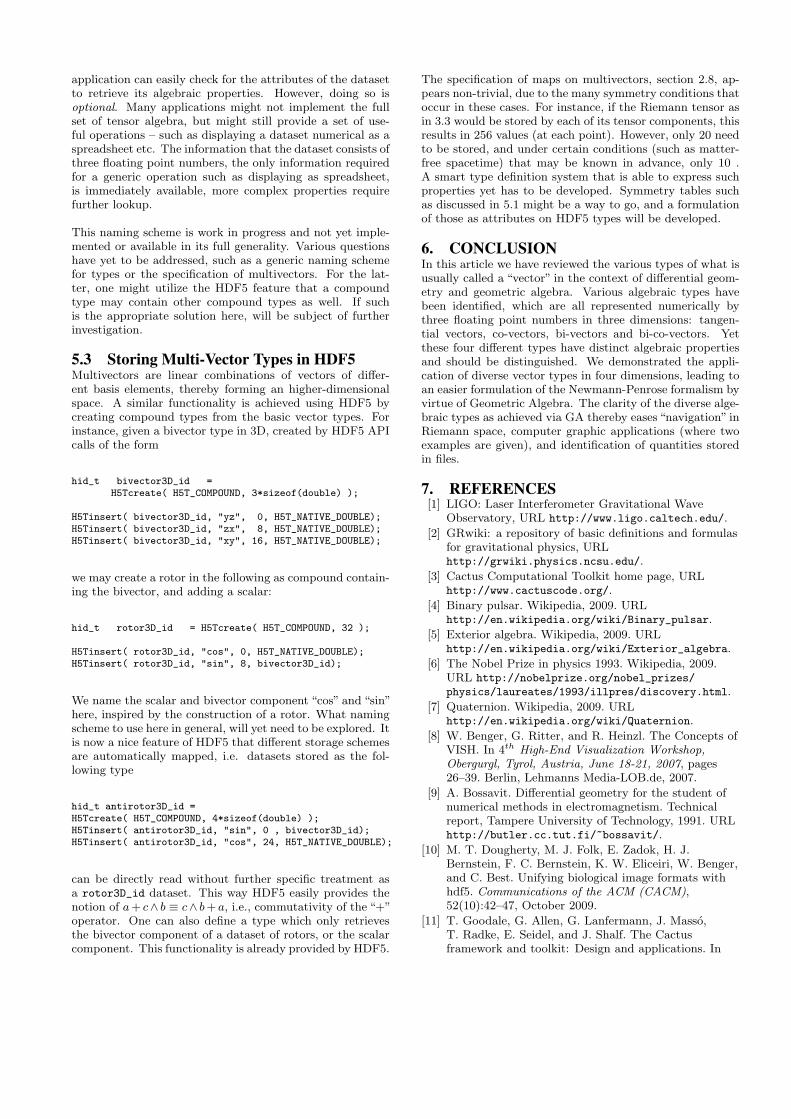
application can easily check for the attributes of the datasetto retrieve its algebraic properties. However, doing so isoptional. Many applications might not implement the fullset of tensor algebra, but might still provide a set of use-ful operations – such as displaying a dataset numerical as aspreadsheet etc. The information that the dataset consists ofthree floating point numbers, the only information requiredfor a generic operation such as displaying as spreadsheet,is immediately available, more complex properties requirefurther lookup.
This naming scheme is work in progress and not yet imple-mented or available in its full generality. Various questionshave yet to be addressed, such as a generic naming schemefor types or the specification of multivectors. For the lat-ter, one might utilize the HDF5 feature that a compoundtype may contain other compound types as well. If suchis the appropriate solution here, will be subject of furtherinvestigation.
5.3 Storing Multi-Vector Types in HDF5Multivectors are linear combinations of vectors of differ-ent basis elements, thereby forming an higher-dimensionalspace. A similar functionality is achieved using HDF5 bycreating compound types from the basic vector types. Forinstance, given a bivector type in 3D, created by HDF5 APIcalls of the form
hid_t bivector3D_id =H5Tcreate( H5T_COMPOUND, 3*sizeof(double) );
H5Tinsert( bivector3D_id, "yz", 0, H5T_NATIVE_DOUBLE);H5Tinsert( bivector3D_id, "zx", 8, H5T_NATIVE_DOUBLE);H5Tinsert( bivector3D_id, "xy", 16, H5T_NATIVE_DOUBLE);
we may create a rotor in the following as compound contain-ing the bivector, and adding a scalar:
hid_t rotor3D_id = H5Tcreate( H5T_COMPOUND, 32 );
H5Tinsert( rotor3D_id, "cos", 0, H5T_NATIVE_DOUBLE);H5Tinsert( rotor3D_id, "sin", 8, bivector3D_id);
We name the scalar and bivector component “cos” and “sin”here, inspired by the construction of a rotor. What namingscheme to use here in general, will yet need to be explored. Itis now a nice feature of HDF5 that different storage schemesare automatically mapped, i.e. datasets stored as the fol-lowing type
hid_t antirotor3D_id =H5Tcreate( H5T_COMPOUND, 4*sizeof(double) );H5Tinsert( antirotor3D_id, "sin", 0 , bivector3D_id);H5Tinsert( antirotor3D_id, "cos", 24, H5T_NATIVE_DOUBLE);
can be directly read without further specific treatment asa rotor3D_id dataset. This way HDF5 easily provides thenotion of a+ c∧ b ≡ c∧ b+ a, i.e., commutativity of the “+”operator. One can also define a type which only retrievesthe bivector component of a dataset of rotors, or the scalarcomponent. This functionality is already provided by HDF5.
The specification of maps on multivectors, section 2.8, ap-pears non-trivial, due to the many symmetry conditions thatoccur in these cases. For instance, if the Riemann tensor asin 3.3 would be stored by each of its tensor components, thisresults in 256 values (at each point). However, only 20 needto be stored, and under certain conditions (such as matter-free spacetime) that may be known in advance, only 10 .A smart type definition system that is able to express suchproperties yet has to be developed. Symmetry tables suchas discussed in 5.1 might be a way to go, and a formulationof those as attributes on HDF5 types will be developed.
6. CONCLUSIONIn this article we have reviewed the various types of what isusually called a “vector” in the context of differential geom-etry and geometric algebra. Various algebraic types havebeen identified, which are all represented numerically bythree floating point numbers in three dimensions: tangen-tial vectors, co-vectors, bi-vectors and bi-co-vectors. Yetthese four different types have distinct algebraic propertiesand should be distinguished. We demonstrated the appli-cation of diverse vector types in four dimensions, leading toan easier formulation of the Newmann-Penrose formalism byvirtue of Geometric Algebra. The clarity of the diverse alge-braic types as achieved via GA thereby eases “navigation” inRiemann space, computer graphic applications (where twoexamples are given), and identification of quantities storedin files.
7. REFERENCES[1] LIGO: Laser Interferometer Gravitational Wave
Observatory, URL http://www.ligo.caltech.edu/.
[2] GRwiki: a repository of basic definitions and formulasfor gravitational physics, URLhttp://grwiki.physics.ncsu.edu/.
[3] Cactus Computational Toolkit home page, URLhttp://www.cactuscode.org/.
[4] Binary pulsar. Wikipedia, 2009. URLhttp://en.wikipedia.org/wiki/Binary_pulsar.
[5] Exterior algebra. Wikipedia, 2009. URLhttp://en.wikipedia.org/wiki/Exterior_algebra.
[6] The Nobel Prize in physics 1993. Wikipedia, 2009.URL http://nobelprize.org/nobel_prizes/
physics/laureates/1993/illpres/discovery.html.
[7] Quaternion. Wikipedia, 2009. URLhttp://en.wikipedia.org/wiki/Quaternion.
[8] W. Benger, G. Ritter, and R. Heinzl. The Concepts ofVISH. In 4th High-End Visualization Workshop,Obergurgl, Tyrol, Austria, June 18-21, 2007, pages26–39. Berlin, Lehmanns Media-LOB.de, 2007.
[9] A. Bossavit. Differential geometry for the student ofnumerical methods in electromagnetism. Technicalreport, Tampere University of Technology, 1991. URLhttp://butler.cc.tut.fi/~bossavit/.
[10] M. T. Dougherty, M. J. Folk, E. Zadok, H. J.Bernstein, F. C. Bernstein, K. W. Eliceiri, W. Benger,and C. Best. Unifying biological image formats withhdf5. Communications of the ACM (CACM),52(10):42–47, October 2009.
[11] T. Goodale, G. Allen, G. Lanfermann, J. Masso,T. Radke, E. Seidel, and J. Shalf. The Cactusframework and toolkit: Design and applications. In

Vector and Parallel Processing – VECPAR’2002, 5thInternational Conference, Lecture Notes in ComputerScience, Berlin, 2003. Springer.
[12] A. J. S. Hamilton and P. P. Avelino. The physics ofthe relativistic counter-streaming instability thatdrives mass inflation inside black holes. PhysicsReports, accepted, 2009. gr-qc/0811.1926.
[13] A. Held. A formalism for the investigation ofalgebraically special metrics. i. Commun. Math. Phys.,37:311–26, 1974.
[14] E. T. Newman and R. Penrose. An approach togravitational radiation by a method of spincoefficients. J. Math. Phys., 3:566–79, 1962.
[15] E. Poisson and W. Israel. Inner-horizon instability andmass inflation in black holes. Phys. Rev.,D41:1796–1809, 1990.
[16] E. (Ted) Newman and R. Penrose. Spin-coefficientformalism. Scholarpedia, 4(6):7445, 2009. URLhttp://www.scholarpedia.org/article/
Newman-Penrose_formalism.
[17] The HDF Group. Hierarchical data format version 5.http://www.hdfgroup.org/HDF5, 2000-2009.
[18] The HDF Group. HDF5 H5T API, 2009. URL http:
//www.hdfgroup.org/HDF5/doc/RM/RM_H5T.html.
[19] T. Veldhuizen. Using C++ template metaprograms.C++ Report, 7(4):36–43, May 1995. Reprinted inC++ Gems, ed. Stanley Lippman.

Evolving Time Surfaces in a Virtual Stirred Tank
Bidur BoharaFarid Harhad
Department of Computer ScienceLouisiana State UniversityBaton Rouge, [email protected],
Werner BengerCenter for Computation &
TechnologyLouisiana State UniversityBaton Rouge, LA-70803
Nathan BrenerS. Sitharama Iyengar
Bijaya B. KarkiDepartment of Computer Science
Louisiana State UniversityBaton Rouge, LA-70803
[email protected]@csc.lsu.edu,[email protected]
Marcel RitterDepartment of Computer Science
University of InnsbruckTechnikerstrasse 21a
A-6020 Innsbruck, [email protected]
Kexi Liu, Brygg UllmerCenter for Computation &
TechnologyDepartment of Computer Science
Louisiana State UniversityBaton Rouge, LA-70803
[email protected], [email protected]
Nikhil Shetty, Vignesh Natesan,Carolina Cruz-Neira
Center for Adv. Comp. StudiesUniversity of Louisiana at
LafayetteLafayette, LA 70504
ABSTRACTThe complexity of large scale computational fluid dynamicsimulations demand powerful tools to investigate the numer-ical results. Time surfaces are the natural higher-dimensionalextension of time lines, the evolution of a seed line of par-ticles in the flow of a vector field. Adaptive refinement ofthe evolving surface is mandatory for high quality underreasonable computation times. In contrast to the lower-dimensional time line, there is a new set of refinement cri-teria that may trigger the refinement of a triangular initialsurface, such as based on triangle degeneracy, triangle area,surface curvature etc. In this article we describe the compu-tation of time surfaces for initially spherical surfaces. Theevolution of such virtual “bubbles” supports analysis of themixing quality in a stirred tank CFD simulation. We discussthe performance of various possible refinement algorithms,how to interface alternative software solutions and how toeffectively deliver the research to the end-users, involvingspecially designed hardware representing the algorithmic pa-rameters.
Keywordsvisualization, CFD, large data, pathlines, timelines, surfacerefinement
1. INTRODUCTION1.1 MotivationComputational Fluid Dynamics (CFD) is a computationally-based design and analysis technique for the study of fluidflow. CFD can provide high fidelity temporally and spatially
resolved numerical data, which can be based on meshes thatrange from a few million cells to tens of millions of cells.The data from CFD can range to several hundred thousandtime steps and be of sizes in order of terabytes.
Therefore, a key challenge here is the ability to easily minethe time dependent CFD data; extract key features of theflow field; display these spatially evolving features in thespace-time domain of interest. In this work, we present aninterdisciplinary effort to generate and visualize time sur-faces of the fluid flow from the time dependent CFD data.The implementation of time surfaces, such as an evolvingsurface of a sphere, for analyzing the flow field is more rele-vant in context of a stirred tank system. The integration ofsurfaces over time generates an evolving surface that can il-lustrate key flow characteristics such as how matter injectedin a stirred tank disperses, and in what regions of the tank isthe turbulence high. Such observations are crucial to iden-tifying the best conditions for optimal mixing.
Figure 1: Two evolving spheres visualized just be-fore their mixing in the Stirred Tank simulation sys-tem.
The CFD dataset was obtained from a large eddy simula-tion (LES) of flow inside a stirred tank reactor (STR). The
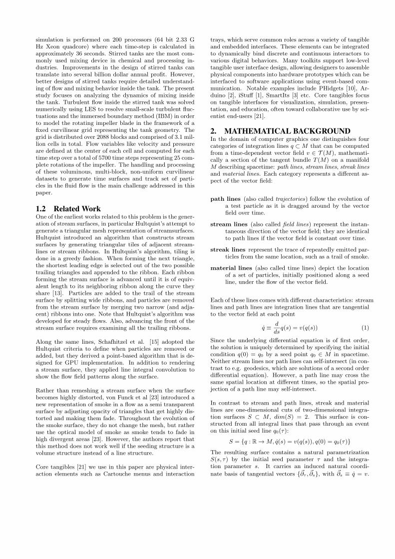
simulation is performed on 200 processors (64 bit 2.33 GHz Xeon quadcore) where each time-step is calculated inapproximately 36 seconds. Stirred tanks are the most com-monly used mixing device in chemical and processing in-dustries. Improvements in the design of stirred tanks cantranslate into several billion dollar annual profit. However,better designs of stirred tanks require detailed understand-ing of flow and mixing behavior inside the tank. The presentstudy focuses on analyzing the dynamics of mixing insidethe tank. Turbulent flow inside the stirred tank was solvednumerically using LES to resolve small-scale turbulent fluc-tuations and the immersed boundary method (IBM) in orderto model the rotating impeller blade in the framework of afixed curvilinear grid representing the tank geometry. Thegrid is distributed over 2088 blocks and comprised of 3.1 mil-lion cells in total. Flow variables like velocity and pressureare defined at the center of each cell and computed for eachtime step over a total of 5700 time steps representing 25 com-plete rotations of the impeller. The handling and processingof these voluminous, multi-block, non-uniform curvilineardatasets to generate time surfaces and track set of parti-cles in the fluid flow is the main challenge addressed in thispaper.
1.2 Related WorkOne of the earliest works related to this problem is the gener-ation of stream surfaces, in particular Hultquist’s attempt togenerate a triangular mesh representation of streamsurfaces.Hultquist introduced an algorithm that constructs streamsurfaces by generating triangular tiles of adjacent stream-lines or stream ribbons. In Hultquist’s algorithm, tiling isdone in a greedy fashion. When forming the next triangle,the shortest leading edge is selected out of the two possibletrailing triangles and appended to the ribbon. Each ribbonforming the stream surface is advanced until it is of equiv-alent length to its neighboring ribbon along the curve theyshare [13]. Particles are added to the trail of the streamsurface by splitting wide ribbons, and particles are removedfrom the stream surface by merging two narrow (and adja-cent) ribbons into one. Note that Hultquist’s algorithm wasdeveloped for steady flows. Also, advancing the front of thestream surface requires examining all the trailing ribbons.
Along the same lines, Schafhitzel et al. [15] adopted theHultquist criteria to define when particles are removed oradded, but they derived a point-based algorithm that is de-signed for GPU implementation. In addition to renderinga stream surface, they applied line integral convolution toshow the flow field patterns along the surface.
Rather than remeshing a stream surface when the surfacebecomes highly distorted, von Funck et al [23] introduced anew representation of smoke in a flow as a semi transparentsurface by adjusting opacity of triangles that get highly dis-torted and making them fade. Throughout the evolution ofthe smoke surface, they do not change the mesh, but ratheruse the optical model of smoke as smoke tends to fade inhigh divergent areas [23]. However, the authors report thatthis method does not work well if the seeding structure is avolume structure instead of a line structure.
Core tangibles [21] we use in this paper are physical inter-action elements such as Cartouche menus and interaction
trays, which serve common roles across a variety of tangibleand embedded interfaces. These elements can be integratedto dynamically bind discrete and continuous interactors tovarious digital behaviors. Many toolkits support low-leveltangible user interface design, allowing designers to assemblephysical components into hardware prototypes which can beinterfaced to software applications using event-based com-munication. Notable examples include PHidgets [10], Ar-duino [2], iStuff [1], SmartIts [3] etc. Core tangibles focuson tangible interfaces for visualization, simulation, presen-tation, and education, often toward collaborative use by sci-entist end-users [21].
2. MATHEMATICAL BACKGROUNDIn the domain of computer graphics one distinguishes fourcategories of integration lines q ⊂M that can be computedfrom a time-dependent vector field v ∈ T (M), mathemati-cally a section of the tangent bundle T (M) on a manifoldM describing spacetime: path lines, stream lines, streak linesand material lines. Each category represents a different as-pect of the vector field:
path lines (also called trajectories) follow the evolution ofa test particle as it is dragged around by the vectorfield over time.
stream lines (also called field lines) represent the instan-taneous direction of the vector field; they are identicalto path lines if the vector field is constant over time.
streak lines represent the trace of repeatedly emitted par-ticles from the same location, such as a trail of smoke.
material lines (also called time lines) depict the locationof a set of particles, initially positioned along a seedline, under the flow of the vector field.
Each of these lines comes with different characteristics: streamlines and path lines are integration lines that are tangentialto the vector field at each point
q ≡ d
dsq(s) = v(q(s)) (1)
Since the underlying differential equation is of first order,the solution is uniquely determined by specifying the initialcondition q(0) = q0 by a seed point q0 ∈ M in spacetime.Neither stream lines nor path lines can self-intersect (in con-trast to e.g. geodesics, which are solutions of a second orderdifferential equation). However, a path line may cross thesame spatial location at different times, so the spatial pro-jection of a path line may self-intersect.
In contrast to stream and path lines, streak and materiallines are one-dimensional cuts of two-dimensional integra-tion surfaces S ⊂ M , dim(S) = 2. This surface is con-structed from all integral lines that pass through an eventon this initial seed line q0(τ):
S = q : R→M, q(s) = v(q(s)), q(0) = q0(τ)
The resulting surface contains a natural parametrizationS(s, τ) by the initial seed parameter τ and the integra-tion parameter s. It carries an induced natural coordi-
nate basis of tangential vectors ~∂τ , ~∂s, with ~∂s ≡ q = v.

For a streak line, the initial seed line q0(τ) is timelike asnew particles are emitted from the same location over time,dq0(τ)/dt 6= 0, for a material line the seed line is spacelikedq0(τ)/dt = 0, a set of points at the same instant of time.The respective streak/time line is the set of points of the sur-face q(t) = St=const. for a constant time. If the integrationparameter is chosen to be proportional to the time s ∝ t,which e.g. is the case when performing Euler steps, then theoriginal seed line parameter τ provides a natural parameterfor the resulting lines, i.e. each point along a time line isadvanced by the same time difference dt at each integrationstep.
Refinement of lines by introducing new integration points ismandatory to sustain numerical accuracy of the results. Theideas of the Hultquist algorithm [12] and its improvementsby Stalling [17] could be applied also to the spatio-temporalcase, however such would result in the requirement to per-form timelike interpolation of the vector field. For data setsthat are non-equidistant in time such as adaptive mesh re-finement data generated from Berger-Oliger schemes [6] find-ing the right time interval for a given spatial location this be-comes non-trivial. For now we refrain from non-equidistantrefinement in the temporal direction (such as done in [14]),though this is an option – if not requirement – for futurework.
A time surface is the two-dimensional generalization of atime line, a volumetric object in spacetime. The Hultquistalgorithm, if applied to a spatio-temporal surface, discussescriteria on refining one edge, whereas here we have a muchricher set of possible surface characteristics that may triggercreation or deletion of integration points. Some options areto refine a surface at locations where
• a triangle’s edge
• a triangle’s area
• a triangle’s curvature
• a triangle degeneration (“stretching”)
becomes larger than a certain threshold. Section 5.1 reviewsour results experimenting with different such criteria.
3. SOLUTION3.1 Data ModelWe use the VISH [4] visualization shell as our implementa-tion platform. It supports the concept of fiber bundles [8]for the data model. The data model consists of seven levels,each of which is comprised of compatible arrays that repre-sent a certain property of the dataset [5]. These levels, whichconstitute a Bundle, are Slice, Grid, Skeleton, Representa-tion, Field, Fragment and Compound. The Field representsarrays of primitive data types, such as int, double, bool, etc.,and the collection of Fields describes the entire Grid. TheGrid objects for different time slices are bundled togetherand are represented as a Bundle. As an example of our im-plementation, each Field contains values of a property suchas coordinates, connectivity information, velocity, etc. Thecollection of these Fields is a Grid object, and the collection
of Grid objects for all time slices is the Bundle of the entiredataset.
The dataset used for visualizing the features of fluid flowcontains numerical data for 2088 curvilinear blocks consti-tuting the virtual stirred tank. The input vector field isfragmented and these fragments are the blocks of the Grid.The input dataset for each time slice consists of coordinatelocation, pressure and fluid velocity for each grid point inthe entire 2088 blocks. These properties are stored as Fieldsin the Grid object for each time slice, and these Grid objectsare then combined into a Bundle.
When a multi-block is accessed for the first time, a Uniform-Grid-Mapper is created which is a uniform grid having thesame size as a world coordinate aligned bounding box of themulti-block. For each cell of the Uniform-Grid-Mapper alist of curvi linear block cells (indices) is stored which inter-sect the Uni-Grid-Mapper cell by doing one iteration over allcurvilinear grid cells and a fast min/max test. When com-puting the local multi-block coordinates the correspondingUni-Grid-Mapper cell is identified first which then selects asmall number of curvilinear cells for the Newton iteration.Uni-Grid-Mapper objects are stored in the Grid object ofthe vector field and can be reused when accessing the samemulti-block again later.
3.2 Out of Core Memory ManagementThe original approach taken while visualizing the featuresof fluid flow is to keep the entire vector field data in themain memory and integrate over the vector field to extractthe features. However, with the necessity of visualizing thetime-dependent 3D vector field, the original approach hasrestrictions, such as the size of the time-dependent data caneasily exceed the capacity of main memory of even state ofthe art workstations. In [24], the authors present the conceptof an out-of-core data handling strategy to process the largetime dependent dataset by only loading parts of the data ata time and processing it. Two major strategies presentedfor out-of-core data handling are Block-wise random accessand Slice-wise sequential access. The authors emphasize theSlice-wise sequential access strategy for handling the datagiven in time slices, however, we have implemented bothBlock-wise access and Slice-wise access of time-dependentdata while generating the time surfaces for visualizing thefluid flow.
Figure 2: Time surface computed from a vector fieldgiven in 2088 fragments (curvilinear blocks) coveringthe Stirred Tank Grid (left). Only those fragmentsthat affect the evolution of the time surface (right)are actually loaded into memory.

Figure 3: Particle advection of a 2-dimensional ele-ment vs. a 1-dimensional element. In our case, oursurface element is in 3-dimensional space spannedover time.
The virtual stirred tank system has 2088 blocks, and eachblock has vector field data for every time slice. The data foreach time slice is accessed only once as a Grid object fromthe input Bundle and processed to generate the time surfaceat that particular time. The integration of the time surfacedoes not process all the blocks, instead only the blocks thatare touched at the given time slice are loaded and processed.
At every time slice two Grid Objects are handled, one con-taining the input data of the vector field and the other con-sisting of seed points and connectivity information amongthe seed points. The connectivity information is used togenerate the triangle mesh for surface generation. In thecase of no surface refinement, the connectivity informationis constant throughout the time slices and is stored once andused multiple times. This conserves the memory and alsoreduces the memory access. However, with surface refine-ment the number of points and their connectivity changesover time resulting in an increase in memory usage.
3.3 Particle Seeding and AdvectionOur set of particle seeds qi,t0 for i = 0, ..., n − 1, lie on asphere. At any given time t > t0, the time surface is repre-sented as a triangular mesh formed by the particles qi,tthathave been advected using equation 1. Figure 3 illustrates thedifference between our seeding approach versus Hultquist’swhere we are evolving a surface element (a triangle) overtime as opposed to spanning a surface out of a line segmentelement.
3.4 Triangular Mesh RefinementsAs time elapses, the triangular mesh of particles enlarges andtwists according to the flow field. To preserve the quality ofthe mesh, we refine it by adding new particles and advectingthem while updating the mesh connectivity. Of the possiblerefinements criteria mentioned above, we have implementedthe following:
Edge length: If the distance between pairwise particles ofa triangle is larger than a threshold edge length, weinsert a new midpoint and subdivide the triangle ac-cordingly.
Triangle area: If the area of the triangle formed by thenew positions of the particle triplet is larger than athreshold area, we insert three midpoints and subdi-vide the triangle to a new set of four adjacent triangles.
4. ALTERNATIVE APPROACHESIn order to verify and compare our results with other imple-mentations, we also investigate alternative implementations.Paraview [11] is one of the well known and widely used vi-sualization tools in the scientific community. It addressesissues pertaining to the visualization of large scale data-setsusing high-performance computing environments. It can beperceived as a framework around the well known Visualiza-tion Toolkit (VTK) [16] library. It not only provides a GUIto VTK, but also provides a convenient environment for in-tuitive visual programming of the visualization pipeline.
Paraview has implicit mechanisms for handling scale, both interms of data and computation [7]. It achieves this by pro-viding generalized abstractions for parallelization and dis-tribution. Therefore a scientist using Paraview can switchfrom visualizing smaller data-sets on a desktop computer toa much larger data-set utilizing a large HPC infrastructure,with minimum effort.
We describe ongoing work and approaches to porting andvisualizing the given F5 (fiber-bundle) data-set, as describedin 3.1, in Paraview.
4.1 Porting the fiber-bundle (F5) to ParaviewThe 500GB fiber-bundle data-set is provided in the F5 for-mat. This format has no native support in Paraview andsome form of conversion would be required to utilize thedata.
One approach to solve this problem is to use a format con-verter and separately convert the entire file to a nativelysupported format. However, this approach causes redun-dant data and can waste considerable amount of space onthe storage disk. An alternative solution is to write a cus-tom reader into Paraview such that the data is read andmapped into internal VTK data-structures. This approachadds an additional computation time into the visualizationpipeline and can cause unnecessary slowdown of the visual-ization process.
An ideal solution would be a combination of the above men-tioned approaches such that both space and time optimiza-tion can be achieved. Such a solution is possible in our casedue to a certain characteristic of the F5 format (explainedshortly) and the use of XDMF (eXtensible Data Model andFormat) [9] which is supported in Paraview.
An F5 format is characteristically a specific description ororganization of the HDF5 data format. All H5 readers andcommands which typically work on HDF5 formats also workon F5.
The XDMF data format is an XML format for data generallyknown as a ”light data”. It provides light weight descriptionsof the ”heavy data” which is typically a HDF5 file containingthe actual data. A XDMF file can thus be seen as an indexinto the HDF5 file and is usually much smaller in size, takingvery less time to get generated.
Paraview is supplied with the generated XDMF file throughwhich it can access the data in the corresponding HDF5(or F5) file. No other reader or converter is necessary. An

added advantage of this approach is that parallel file readers(if supported) and other parallel algorithms can be used toquickly access and process very large data-sets. We thusleverage on the parallel and distributed framework alreadyprovided in Paraview.
4.2 Details of XDMF for F5 fiber-bundleAn XDMF description of the F5 fiber-bundle is shown below.
<?xml version="1.0" ?>
<!DOCTYPE Xdmf SYSTEM "Xdmf.dtd" [
<!ENTITY HeavyData "50New.f5">
]>
<Xdmf Version="2.0">
<Domain>
<Grid Name="TimeSeries" Type="Temporal">
<Grid Name="Multiblock" Type="Spatial">
<Time Value="000000000.0000000000"/>
<Grid Name="Block00001">
<Topology TopologyType="3DSMesh"/>
<Geometry>
<DataItem Format="HDF">
&HeavyData;:/f5/path/to/Points/Block00001
</DataItem>
</Geometry>
<Attribute Name="Pressure">
<DataItem Format="HDF">
&HeavyData;:/f5/path/to/Pressure/Block00001
</DataItem>
</Attribute>
<Attribute Name="Velocity">
<DataItem Format="HDF">
&HeavyData;:/f5/path/to/Velocity/Block00001
</DataItem>
</Attribute>
</Grid>
<Grid Name="Block00002">
...
</Grid>
</Grid>
<Grid Name="TimeSeries" Type="Temporal">
<Grid Name="Multiblock" Type="Spatial">
<Time Value="000000001.0000000000"/>
....
....
</Grid>
</Grid>
</Domain>
</Xdmf>
As seen in the description above, the XDMF consists of acollection o f Temporal-Grids which represents each timestep. Each Temporal-Grid contains a collection of Spatial-Grids which is a representation of multiblock data. Eachmultiblock data consists of curvilinear blocks. The data forthese blocks are in the HDF5 file specified within DataItems.
As of now, results from the Paraview approach are still pend-ing and subject of further investigation.
5. RESULTS5.1 Surface RefinementFor the different refinement criteria test cases, we bench-marked our implementation with a 30-timestep subset (85MB per timestep) of the stirred tank data and on a 64-bitdual core (2GHz each) pentium laptop machine with 4GBof RAM. We advected one sphere for the first 30 timestepsof the simulation. Due to the small size of our test data,we could not notice a difference in time surface meshingquality from the visualization itself, but from the data intables 1 and 2, we notice a slight performance improvementof the area criteria over the edge length criteria. Thoughthe number of particles is slightly higher in the second case,this suggests that the quality of the surface with the areacriterion is better.
threshold tot points avg time/slice(sec) tot time(sec)0.005 4269 6.480 200.8680.01 822 1.519 47.10.02 258 1.165 36.101
Table 1: Timing Analysis for Edge Length Criteria
threshold tot points avg time/slice(sec) tot time(sec)0.005 4269 6.864 212.7850.01 837 1.454 45.080.02 258 1.150 35.646
Table 2: Timing Analysis for Triangle Area Criteria
From either tables 1 or 2, picking a threshold too small com-pared to the characteristic of the triangle being examined,results in maximum refinement, while a large enough thresh-old leads to no refinement at all.
5.2 Timing AnalysisFor the overall integration and refinement of the time sur-face, we used a larger dataset of size 12GB with 150 timesteps.We ran the implementation on a 64bit quadcore workstationwith 64 GB of RAM. We used the edge length criterion witha threshold of 0.01.
time no. of points time for slice(sec) time/point(ms)0 516 0.4 7.050 3468 2.0 5.9100 15822 7.4 4.8125 41574 18.8 4.7150 129939 49.7 4.0
Table 3: Timing Analysis for Threshold=0.01
The listing in the above table is for 12 GB of input datafrom an initial time of 0 to a final time of 150. Initially thenumber of points is 516, which increases over time as morepoints are generated for surface refinement. As the numberof points increases, the computation time for the next timeslice increases. However, the time per point seems to beslowly decreasing. This may be because more and morepoints tend to locate in the same block and the data of oneblock is shared by many points, resulting in less memoryaccess per point.

Figure 4: Images showing evolution of two spheresat time slices 0, 50, 100, 125 and 150, respectivelyfrom left-top to bottom, as seen top-view of thestirred tank. First image shows the seed spheres,and the last image shows two sphere just before thesurfaces are about to mix.
6. DEPLOYMENT TO END USERSResults of the algorithm can be investigated better if we ex-plore the entire time evolution of the surface interactively,by navigating through space and time. In most visualizationenvironments, the graphical user interface is tightly coupledwith the underlying visualization functionality. One featureof VISH is that it decouples the interface from the under-lying visualization application. At least in principle, thismakes it as easy to couple VISH to a CAVE immersive en-vironment, a web based distributed interface, or physicalinteraction devices as to the provided traditional 2D graph-ical user interface. As an example of this, we have based asignificant portion of our interaction with the present largedataset from stirred tank with “viz tangible” interaction de-vices. An example of this is pictured in Figure 5. Earlierstages of this work have been described in [22, 20, 19, 18].
An application programming interface (API) is under de-velopment which supports coupling tangibles to VISH andother visualization environments. In this API, when interac-tion control messages are sent (triggered by physical events,such as RFID entrance/exit or the turning of a knob), theytrigger corresponding methods in VISH. We use cartouches –
Figure 5: User physically manipulating VISH appli-cation through “viz tangibles” interaction devices
RFID-tagged interaction cards [19, 20] – as physical interac-tors which describe data and operations within the VISH en-vironment. Users can access, explore and manipulate datasetsby placing appropriate cartouches on an interaction tray(Figures 5, 6), and making appropriate button presses, wheelrotations, etc.
Figure 6: Cartouche cards for viewpoint control andparameter adjustment operations
In our present implementation, we have used two classes ofcartouche objects. These are summarized below:
1. Viewpoint operations: Specific supported view pointcontrols include rotation, zooming, and translation. Inthe case of rotation and translation, individual wheelsare bounds to the (e.g.) x, y, z axis. In the contextof zooming or time step navigation, wheels representdifferent scales of space and time navigation.
2. Parameter Adjustment operations: Our current imple-mentation includes time surface seedings and surfacetransparency adjustment. For time surface seedings,we steer center of seeds, number of subdivisions, etc.

to parameter wheels. Within surface transparency ad-justment, wheels are bounded to different scales of sur-face transparency.
In future, we hope quantities in high dimensional parameterspace such as curvature and torsion of the surface can alsobe explored effectively with the integration of “viz tangibles”and the API.
7. CONCLUSIONWhile most of the previous visualization techniques for fluidflow have concentrated on flow streamlines and pathlines,our approach has been directed towards generating the timesurfaces of the flow. The interdependencies of integrationover a vector field require random access to amounts ofdata beyond a single workstation’s capabilities, while atthe same time requiring shared memory for required refine-ments. This limits available hardware and impacts paral-lelization efforts. The evolution of a seed surface requiredrefinement of its corresponding triangular mesh to preservethe quality of the time surface over time. From the resultswe noticed a slight superior quality of the area refinementcriterion over the edge length criterion.
8. ACKNOWLEDGMENTSWe thank the VISH development team, among them GeorgRitter, University of Innsbruck, and Hans-Peter Bischof,Rochester Institute of Technology, for their support; Ami-tava Jana and Sanjay Kodiyalam from Southern University,Baton Rouge for their continued vision for interactive us-age in the CAVE VR environment by providing resources todrive further development and optimization of the softwareenvironment. This research employed resources of the Cen-ter for Computation & Technology at Louisiana State Uni-versity, which is supported by funding from the Louisianalegislature’s Information Technology Initiative. Portions ofthis work were supported by NSF/EPSCoR Award No. EPS-0701491 (CyberTools), NSF MRI-0521559 (Viz Tangibles)and IGERT (NSF Grant DGE-0504507).
9. ADDITIONAL AUTHORSAdditional authors: Sumanta Acharya and Somnath Roy,Department of Mechanical Engineering, at Louisiana StateUniversity; [email protected],[email protected].
10. REFERENCES[1] R. Ballagas, M. Ringel, M. Stone, and J. Borchers.
iStuff: a physical user interface toolkit for ubiquitouscomputing environments.
[2] M. Banzi. Getting Started with Arduino. Make Books -Imprint of: O’Reilly Media, Sebastopol, CA, 2008.
[3] M. Beigl and H. Gellersen. Smart-its: An embeddedplatform for smart objects. In Smart ObjectsConference (sOc), volume 2003. Citeseer, 2003.
[4] W. Benger, G. Ritter, and R. Heinzl. The Concepts ofVISH. In 4th High-End Visualization Workshop,Obergurgl, Tyrol, Austria, June 18-21, 2007, pages26–39. Berlin, Lehmanns Media-LOB.de, 2007.
[5] W. Benger, M. Ritter, S. Acharya, S. Roy, andF. Jijao. Fiberbundle-based visualization of a stir tankfluid. In WSCG 2009, Plzen, 2009.
[6] M. J. Berger and J. Oliger. Adaptive mesh refinementfor hyperbolic partial differential equations. J.Comput. Phys., 53:484–512, 1984.
[7] J. Biddiscombe, B. Geveci, K. Martin, K. Morel, andD. Thompson. Time dependent processing in aparallel pipeline architecture. IEEE Transactions onVisualization and Computer Graphics, 13:2007.
[8] D. M. Butler and M. H. Pendley. A visualizationmodel based on the mathematics of fiber bundles.Computers in Physics, 3(5):45–51, sep/oct 1989.
[9] J. A. Clarke and R. R. Namburu. A distributedcomputing environment for interdisciplinaryapplicationsaAI, concurrency and computation:Practice and experience vol. 14, grid computingenvironments special issue. Currency andComputation: Practice and Experience, (14):13–15,2002.
[10] S. Greenberg and C. Fitchett. Phidgets: easydevelopment of physical interfaces through physicalwidgets. In Proceedings of the 14th annual ACMsymposium on User interface software and technology,pages 209–218. ACM New York, NY, USA, 2001.
[11] A. Henderson. Paraview guide, a parallel visualizationapplication, 2005.
[12] J. P. Hultquist. Constructing stream surfaces insteady 3d vector fields. In Visualization ’92, pages171–178. IEEE Computer Society, 1992.
[13] J. P. M. Hultquist. Constructing stream surfaces insteady 3d vector fields. In VIS ’92: Proceedings of the3rd conference on Visualization ’92, pages 171–178,Los Alamitos, CA, USA, 1992. IEEE ComputerSociety Press.
[14] H. Krishnan, C. Garth, and K. I. Joy. Time and streaksurfaces for flow visualization in large time-varyingdata sets. Proceedings of IEEE Visualization ’09, Oct.2009.
[15] T. Schafhitzel, E. Tejada, D. Weiskopf, and T. Ertl.Point-based stream surfaces and path surfaces. In GI’07: Proceedings of Graphics Interface 2007, pages289–296, New York, NY, USA, 2007. ACM.
[16] W. Schroeder, K. Martin, and W. Lorensen. Thevisualization toolkit: An object oriented approach to3d graphics, 1996.
[17] D. Stalling. Fast Texture-Based Algorithms for VectorField Visualization. PhD thesis, Free UniversityBerlin, 1998.
[18] C. Toole, B. Ullmer, R. Sankaran, K. Liu,S. Jandhyala, C. W. Branton, and A. Hutanu.Tangible interfaces for manipulating distributedscientific visualization applications. Submitted to Proc.of TEI’10, 2010.
[19] B. Ullmer, Z. Dever, R. Sankaran, C. Toole,C. Freeman, B. Casady, C. Wiley, M. Diabi, A. J.Wallace, M. Delatin, B. Tregre, K. Liu, S. Jandhyala,R. Kooima, C. W. Branton, and R. Parker. Cartouche:conventions for tangibles bridging diverse interactivesystems. Submitted to Proc. of TEI’10, 2010.
[20] B. Ullmer, A. Hutanu, W. Benger, and H.-C. Hege.Emerging tangible interfaces for facilitatingcollaborative immersive visualizations. NSF LakeTahoe Workshop on Collaborative Virtual Reality andVisualization, 2003.
[21] B. Ullmer, R. Sankaran, S. Jandhyala, B. Tregre,C. Toole, K. Kallakuri, C. Laan, M. Hess, F. Harhad,U. Wiggins, et al. Tangible menus and interactiontrays: core tangibles for common physical/digitalactivities. In Proceedings of the 2nd internationalconference on Tangible and embedded interaction,pages 209–212. ACM New York, NY, USA, 2008.
[22] B. Ullmer, R. Sankaran, S. Jandhyala, B. Tregre,C. Toole, K. Kallakuri, C. Laan, M. Hess, F. Harhad,U. Wiggins, and S. Sun. Tangible menus andinteraction trays: core tangibles for commonphysical/digital activities. In Proc. of TEI ’08, pages209–212, 2008.
[23] W. von Funck, T. Weinkauf, H. Theisel, and H.-P.Seidel. Smoke surfaces: An interactive flowvisualization technique inspired by real-world flowexperiments. IEEE Transactions on Visualization andComputer Graphics (Proceedings Visualization 2008),14(6):1396–1403, November - December 2008.
[24] T. Weinkauf, H. Theisel, H.-C. Hege, and H.-P. Seidel.Feature flow fields in out-of-core settings. InH. Hauser, H. Hagen, and H. Theisel, editors,Topology-based Methods in Visualization, Mathematicsand Visualization, pages 51–64. Springer, 2007.Topo-In-Vis 2005, Budmerice, Slovakia, September 29- 30.