Computing discrete logarithms

with special linear systems

Claus Diem and Sebastian Kochinke

October 11, 2013

Abstract

The idea to compute discrete logarithms in degree 0 class groups ofnon-singular proper non-hyperelliptic curves of a fixed genus over finitefields with the help of special linear systems is studied. On the basisof this general idea new algorithms for the discrete logarithm problemfor curves of a fixed genus g at least 5 over finite fields Fq are given. Itis argued heuristically that for most curves, the problem can be solved

in an expected time of O(q2− 2

d g+12

e). It is also shown with experiments

that with a suitable algorithm one can compute discrete logarithms forcurves of genus 5 with known order of the degree 0 class group just asefficiently as one can compute discrete logarithms for curves of genus4 with the previously most efficient practical algorithm.

1 Introduction

This work is a study on the use of special linear systems to compute discrete

logarithms in class groups (or Picard groups) of non-singular, proper non-

hyperelliptic curves of a fixed genus over finite fields.

Given an instance of the discrete logarithm problem with a curve Cover a finite field Fq, we want to use the usual index calculus or relation

generation and linear algebra method to compute the discrete logarithm;

see e.g. [EG02].

Our starting point is the following observation: Essentially by definition,

all divisors in a linear system of the curve are linearly equivalent. One might

therefore try to compute relations by considering linear systems on the curve.

A further observation is that it is advantageous for the algorithm to consider

systems whose dimension is particularly large with respect to their degree.

One is therefore lead to the idea to consider complete linear systems with

particularly large degree of speciality.

We are both interested in theoretical, complexity theoretic aspects of

the mentioned computational problem as well as in practical computations.

1

So, we discuss both these aspects and give various algorithms based on the

general idea to use complete special linear systems.

Before we present the main new contributions, we briefly mention the

most important previous results.

First, in [Die11] it is shown that one can solve the discrete logarithm

problem for curves of a fixed genus g ≥ 2 in an expected time of

O(q2− 2

g ) . (1)

Moreover, in [Die06] it is argued heuristically that one can solve the discrete

logarithm problem for nearly all curves of a fixed genus g ≥ 3 in an expected

time of

O(q2− 2

g−1 ) . (2)

Here by “nearly all curves” we mean that the fraction of isomorphism classes

of curves for which the result does not apply converges to 0 for q −→ ∞.

The algorithm does however not apply to hyperelliptic curves.

From a theoretical point of view, our main contribution is the following

asymptotic result which is based on some heuristic assumptions.

Heuristic Result Let a natural number g ≥ 3 be fixed. Then the discrete

logarithm problem for nearly all curves of genus g can be solved in an expected

time of

O(q2− 2

d g+12 e). (3)

This improves upon (2) for g ≥ 5.

From a practical point of view the first bottleneck in all algorithms for

the results mentioned is the computation of the group order. But even if

the group order is known our algorithm for the above “Heuristic Result” is

not practical at all. However, we give a further algorithm which is indeed

practical provided that the group order or at least the order of the subgroup

in which the computation takes place is known and provided that the genus

is not too large with respect to the size of the ground field. For this algorithm

we argue heuristically that the expected running time is

O(q2− 2

g−2 ) (4)

for nearly all curves of a fixed genus g ≥ 5. Note here that (4) is equal to

(3) for g = 5 and for g = 6.

We demonstrate experimentally that the explicit running times for curves

of genus g = 5 or 6 the running times are comparable to the running time of

the previous algorithm in [Die06] for a curve of genus g−1 (that is, g−1 = 4

resp. 5).

2

We now give some information how the results mentioned above can be

obtained.

For (1) the method of double large prime variation is used, a method

which also comes into play in this work. The relation generation takes

place by considering random elements in the degree 0 divisor class group of

the curve. This means that the generation of relations relies on factoring

effective divisors which are of degree g most of the time.

In [Die06] an algorithm is given which is based on the following idea:

Let us assume that the curve is given by a possibly singular curve in the

projective plane. (We call such a curve a (birational) plane model of the

original curve.) Then we can compute relations by intersecting the non-

singular part of the plane model by lines. It is argued heuristically that for

curves given by plane models of a fixed degree d one can solve the discrete

logarithm problem in an expected time of

O(q2−2

d−2 ) . (5)

Denoting by ω the canonical sheaf on the curve, for any effective divisor

D of degree g − 3 on the curve, the complete linear system |ω(−D)| has

degree g + 1 and dimension at least 2. Geometric arguments suggest that

for nearly all effective divisors on nearly all curves, the system is base-point

free of dimension 2 and defines a morphism to P2Fq

which is birational onto

its image. Applying the algorithm to this morphism and the plane model

defined by it, we obtain the heuristic expected running time given in (2).

For any non-hyperelliptic curve of genus 3 the canonical linear system

itself defines an embedding into the projective plane, giving a non-singular

plane curve of degree 4. Heuristically, one can then obtain an expected

running time of O(q). In [Die12a] it is proven that one can indeed obtain

this expected running time. In the same work, it is also proven that one

can obtain an expected running time like in (5) if some other conditions are

satisfied.

We come to the use of special linear systems to compute relations. We

note that the number d−2 in formula (5) is the difference between the degree

and the dimension of the linear system “cut out by lines”. Provided that the

linear system defining the morphism to P2Fq

is complete, by Riemann-Roch,

we have d− 2 = g − i, where i is the index of speciality. The expected time

given in (5) can then also be stated as

O(q2− 2

g−i ) . (6)

We see here that the idea to consider special invertible sheaves and the

associated complete linear systems is already present in the works [Die06]

and [Die12a].

3

A further insight is that for any invertible sheaf L and any effective

divisor D, the index of speciality of L(−D) is at least the index of speciality

of L. This observation suggests to follow the general idea that “the smaller

the dimension the better” and more concretely to consider complete linear

systems of dimension 1. A further confirmation of this general idea is given

by Brill-Noether theory for special linear systems. The algorithm for the

“Heuristic Result” is based on the consideration of such systems which are

in turn computed by solving multivariate polynomial equations.

The practical algorithm mentioned above which heuristically leads to the

expected running time given in (4) for g ≥ 5 can be seen as a variant of the

algorithm in [Die06]. As the algorithm for the “Heuristic Result” above, it

is based on complete linear systems of dimension 1. A brief outline is as

follows: As above, we consider effective divisors D of degree g − 3 and the

associated complete linear systems |ω(−D)|. As mentioned, one can expect

that such a linear system defines a plane model of degree g+ 1 of the curve.

For g ≥ 4 these models are singular. Let us assume that we have a plane

model with a rational singularity. Then we consider the pencil defined by

the lines through such a singularity. The degree of this pencil is now at most

g − 1 instead of g for the pencils through non-singular points. In contrast

to the algorithm in [Die06], now one plane model is not enough to solve

the discrete logarithm problem. We therefore vary the effective divisor D.

Using Brill-Noether theory, we argue that for g ≥ 5 the algorithm operates

as desired for nearly all curves.

Overview

In the next section we discuss the representation of the objects we consider

in this work as well as basic computations. In the third section we present

ideas for the computation of discrete logarithms in degree 0 class groups

of curves of a fixed genus via the index calculus method and special linear

systems. Building on geometric considerations of the third section, in the

forth and the last section we show how one can use results and methods from

Brill-Noether theory for our applications. Here we start with an overview

over the results of the theory. Then we give four methods to compute

special linear systems and discuss their application to the computation of

discrete logarithms. The first, “basic”, method is elementary. The second,

“general”, method is based directly on the methods of Brill-Noether theory

and leads to the “Heuristic Result” stated above. The third method leads

to the practical algorithm mentioned above which has been already briefly

outlined. The last method is a particular method from the literature to

compute birational plane models of degree 6 of curves of genus 6. We end

4

the work with experimental results on the second method for curves of genus

5 and 6 and a comparison with the algorithm in [Die06].

2 Geometric background and representation of ob-jects

2.1 Some basic definitions and notations

We use the notation that N = {1, 2, . . .} and N0 = {0, 1, 2 . . .}.We use the following notation from [Die06] and [Die12a]: Let X be an

infinite countable set and (ax)x∈X , (bx)x∈X ∈ RX with bx > 0 for all x ∈ X.

Then we write ax & bx if lim infx∈X

axbx≥ 1.

For a field k, we set P2k := Proj(k[X,Y, Z]), and we set x := X

Z , y := YZ .

A curve over a field k is always assumed to be geometrically integral

but not necessarily proper or regular. Additionally, we fix the following

terminology: For any non-negative integer g, a curve of genus g is a proper

and regular curve of genus g. Recall that over a perfect field k, a curve

is regular if and only if it is smooth. We then also say that the curve is

non-singular.

In the following we will consider algorithms for curves over finite fields.

The input will always consist of a non-singular proper curve over a finite

field and some additional data. In the corresponding complexity-theoretic

statements, we will denote the genus of the curve by g and the cardinality

of the ground field by q.

2.2 Basic representations and computations

By [Heß05, Theorem 56] a curve of genus g over a finite field has a birational

plane model of degree O(g). We represent the curves by such models. In turn

such a model over a finite field k is represented by a homogeneous defining

polynomial F (X,Y, Z) ∈ k[X,Y, Z]. Explicitly this means that to give a

curve of genus g over a finite field k means to give a homogeneous polynomial

F ∈ k[X,Y, Z]. This polynomial defines a plane curve Cpm, and we have the

normalization π : C −→ Cpm, where C is a (non-singular) curve of genus g and

π is birational. As the curve C is proper, it is projective. However, at least a

priori we do not need a representation of C by homogeneous equations, and

we do not need defining equations of affine parts either.

We identify the non-singular locus of Cpm with its preimage in C, and

in particular we identify the function fields of C and Cpm. We denote the

functions induced by x and y on C by x|C and y|C .

5

If not stated otherwise, to represent divisors on such a curve C, we follow

the ideal theoretic approach described in [Heß01]. We give some brief infor-

mation on this approach which we need in the following; besides in [Heß01]

further information on this approach can be found in [Die11]. We assume

that the extension k(C)|k(x|C) is separable; if this is not the case, one can

interchange x and y to achieve this. Now, with f(x, y) := F (X,Y,Z)

Zdeg(F ) , one has

k(C) = k(x|C)[y]/(f(x|C , y)). Let m := deg(f). A rational function on C,that is, an element of the function field k(C) is given in a unique way in the

form∑m−1

i=0 ai(x|C)yi|C with ai(x) ∈ k(x) for i = 0, . . . ,m− 1. We represent

such a function by what we call its coefficient vector (ai(x))m−1i=0 ∈ k(x)m.

To study the complexity of algorithms, we define the height of the coeffi-

cient vector of a function as the maximum of the degrees of the entries of

its coefficient vector, considered as rational functions.

One now considers the closures of k[x|C ] and k[ 1x|C

]( 1x|C

) in k(C). Ev-

ery divisor is represented by two broken ideals with respect to these two

orders. Based on appropriate representations following this idea, negation

and addition of divisors, computation of infima and suprema of two divi-

sors, computation of Riemann-Roch spaces (L-spaces) of divisors and the

computation of a canonical divisor can be performed in polynomial time in

log(q), g and the height of the divisors.

Here the algorithm to compute the L-space of a divisor D outputs a

basis consisting of functions such that the heights of the coefficient vectors

are polynomially bounded in the height of D and g. If one applies this to

principal divisors of functions, one sees that the height of the coefficient

vector of a function is polynomially bounded in the degree of the function

and g. From this it follows that the computation of a principal divisor of a

function can be performed in a time which is polynomially bounded in the

degree of the function, g and log(q).

In our index calculus algorithms, we will always consider curves of a fixed

genus. Therefore, for q large enough, every curve has a k-rational point. To

represent divisor classes on a non-singular proper curve, we fix a rational

point P0 on the curve. We call an effective divisor D P0-reduced if the linear

system |D−P0| is empty. (In [Heß01] and [Die11] the divisor D is then called

reduced along P0.) Now, a divisor class a is represented by its degree and the

unique P0-reduced divisor D with a = [D]− (deg(D)− deg(a)) · [P0]. With

this representation, the computation in the degree 0 divisor class group can

be performed in polynomial time in log(q) and g with the basic operations

on divisors mentioned above.

For the index calculus algorithms, we also have to consider divisors in

factorized representation. Again following [Heß01], we speak of divisors in

free representation. One possibility for a free representation is to represent

6

the prime divisors also in ideal representation. If not stated otherwise we

consider this representation if we talk about the free representation of a

divisor. This free representation of a divisor can be computed in expected

polynomial time in log(q) and the height of the divisor with a randomized

algorithm.

We are particularly interested in effective divisors which split completely

into rational points. One can identify all non-singular points of Cpm with

their preimages in C. Like this, all rational points of C not lying over sin-

gular points can be represented by the corresponding coordinates. This

representation is particularly interesting for some applications.

2.3 Linear systems and their representations

All new algorithms in this work are related to linear systems on non-singular

proper curves over finite fields. We therefore now recall some basic facts

concerning linear systems on proper regular curves, fix some terminology

and notation and describe ways to represent linear systems and to compute

divisors in linear systems. For the computational aspects, we always con-

sider linear systems on curves over finite fields. The geometric aspects hold

however for arbitrary proper regular curves.

Let C be a proper regular curve over some field k. Let K be the sheaf

of meromorphic functions on C (which is a constant sheaf). For an invert-

ible sheaf L on C and a meromorphic section s of L (that is, an element

of Γ(C,K ⊗OL)), we have the associated divisor of zeroes divL(s). The

homomorphism K −→ K ⊗O L given by 1 7→ s induces an isomorphism

O(divL(s)) −→ L. In particular, all divisors of zeroes of meromorphic sec-

tions of L define the same element in the Picard group of C, namely L.

For a vector subspace V of Γ(C,L) we have the associated linear system

d consisting of the divisors of zero of sections in V . Via the canonical

map V −→ d the system is a projective space (in the sense of elementary

geometry), in particular we can talk about the dimension of the system.

Here, the dimension of the empty space is −1. For V = Γ(C,L) we obtain the

complete linear system |L| of L. For a divisor D we have |O(D)| = |D|, the

set of divisors linear equivalent to D. We define the dimension of a divisor as

the dimension of the associated complete linear system. We remark that we

never talk about the dimension of an invertible sheaf. We also remark that

if a linear system d is non-empty, the tuple (L, V ) is uniquely determined

by d up to isomorphism.

Let now L be an invertible sheaf on C and let D be a divisor. As usual, we

set L(D) := L⊗OO(D). The injection O(D) ↪→ K induces an isomorphism

K ⊗OO(D) −→ K. It follows that K ⊗OL(D) is canonically isomorphic

to K ⊗OL. We can therefore regard every meromorphic section of L as a

7

meromorphic section of L(D). We have here divL(D)(s) = divL(s) + D. In

particular, for f ∈ k(C) = Γ(C,K), divO(D)(f) = (f) +D.

Let now D be an effective divisor. Then L(−D) is a subsheaf of L and

|L(−D)| = {E ≥ 0 | E +D ∈ |L|}. In analogy to this, we set for any linear

system d

d(−D) := {E ≥ 0 | E +D ∈ d} .

Let d be defined by (L, V ). Then d(−D) is defined by (L(−D), V ∩Γ(C,L(−D))),

where we again identify meromorphic sections of L with meromorphic sec-

tions of L(−D). Thus d(−D) is again a linear system.

For any effective divisor D, the set d + D is also a linear system: It is

given by (L(D), V ). The base locus B of a linear system d is the scheme-

theoretic intersection of all divisors in d — one can also say that it is the

infimum of the set d in the set of all divisors. We have d(−B) +B = d.

Finally we recall that for every morphism π : C −→ Prk whose image is

not contained in a hyperplane, the pull-back of hyperplanes via π defines

a base point free linear system of dimension r on C, and conversely, every

base point free linear system on C of dimension r arises in this way and

determines the morphism up to an automorphism of Prk.

The following ways to represent a non-empty linear system on a curve Cover a finite field k come to mind.

a) One represents the system by an effective divisor D in the system and a

basis of the vector subspace V of L(D) = Γ(C,O(D)) defining the system.

b) In case the system is complete: One represents the system by an effective

divisor in the system. (That is, in contrast to a), one can drop the basis

of V .)

c) If the system is base point free: One represents the system as in a) but one

can now drop the divisor D. Note that any basis of V defines a morphism

to Prk, and the system is now given by pull-back of the hyperplanes in

Prk.

We also note that we have the following special case for base point free

systems: Let C itself be represented by a plane model Cpm. We recall that

this means that C is the normalization of Cpm and by definition we have a

canonical birational morphism π : C −→ Cpm. Then the lines in P2k define a

base point free system on C. If we follow the representation in c), the system

can be represented by the system of functions x, y, 1.

These representations lead to the computation of divisors in linear sys-

tems: With representation a), to compute a random divisor in the system or

to enumerate the divisors, one can consider linear combinations of the basis

8

elements. If f is such a function, one considers (f) + D. The computation

can be performed in polynomial time. Starting with representations b) and

c), one can first compute a representation as in a) in polynomial time in

log(q), g and the degree of D and then proceed as indicated.

Furthermore, in all three representations, given a linear system d on a

curve and an effective divisor D, the system d(−D) can also be computed

in polynomial time in log(q), g and the degree of d.

For the index calculus algorithms we consider, we want to check quickly

if a divisor in a linear system splits completely into rational points and if

so, we want to compute the divisor in free representation.

One possibility for this is the ideal theoretic approach mentioned above.

We call this the implicit approach.

If one is given a base point free system which defines a morphism ϕ to

Prk which is birational onto its image, one can also consider the following

approach: One first computes the image of the curve under ϕ. (For this

see subsection 2.4.4 below.) One now represents the rational points on the

curve lying over non-singular points by corresponding points in Prk, that is,

by their coordinates. The elements of the linear system are then given by

hyperplanes. For the hyperplanes which intersect the image in non-singular

points, the corresponding divisors are then given by intersection with ϕ(C).We call this the explicit approach.

The explicit approach is particularly important for r = 2, which means

exactly that ϕ(C) is a plane model of C. As already mentioned, the algo-

rithms in [Die06], [Die12a] are based on the intersection of the plane model

with lines. For this approach it is advisable to first try to compute a plane

model of small degree and transfer the discrete logarithm problem to the

new plane model. As mentioned, the practical algorithm which heuristically

leads to the expected running time in (4) involves several different plane

models. We will give, in subsection 4.2.3, two variants of the algorithm, one

based on the implicit and one based on the explicit approach.

2.4 Computations with morphisms

We now discuss the computation with morphisms from a non-singular proper

curve over a finite field to a projective space.

2.4.1 Linear relations between functions

A problem which is basic for the following computations is as follows:

Given a non-singular proper curve C over a finite field k and a system

of functions f1, . . . , fn on C, compute all linear relations between f1, . . . , fn,

that is, compute a basis of the space of tuples a ∈ kn with a1f1 + · · · +

9

anfn = 0. There is a straightforward solution to this based on the coefficient

vectors of the functions: After multiplication with a common denominator

one obtains a system of linear equations over k[x] with indeterminates over

k, and this in turn leads to a linear system of equations over k.

As we stated above, the height of the coefficient vector of a function is

polynomially bounded in the degree of the function and g. Because of this,

the number of equations of the linear system to be solved is polynomially

bounded in the degrees of the functions, n and g. It follows that the com-

putation can be performed in a time which is polynomially bounded in the

degrees of the functions, n, g and log(q).

We also mention that in practice, one might also use the following al-

ternative method: One specializes the equation a1f1 + · · · + anfn = 0 at

more than n randomly chosen rational points of the plane model – provided

of course that such points exist. Note here that the points might even be

singular points of the plane model. The points are represented by their co-

ordinates. At each point one tries to evaluate the elements of the coefficient

vector. This process fails if one of the denominator vanishes, otherwise,

one obtains the value of the function at the point. This procedure might

of course output a space which is larger than the space of relations to be

computed, but in practice it works very well.

2.4.2 Images of points

Above, we already considered the task to compute the image of a rational

point under a function. However, the solution was not completely general.

A general solution to the computation of the image of such a point has been

given in Section 5 of [Die12b]. We recall this solution:

Let a non-singular proper curve C over a finite field k, a non-trivial

function f on C and a rational point P of C be given. Here the point shall

be represented by the associated prime divisor, which means explicitly that

it is given by an ideal in an order.

We first test whether P is a pole at f by computing inf{(f)∞, P}. Let

us assume that this is not the case.

Now f(P ) is the unique element a ∈ k such that f − a vanishes at P .

All functions f − a lie in L((f)∞), and they lie in L((f)∞ − P ) if and only

if a = f(P ).

The computation is now as follows: We compute a basis b1, . . . , b` of

L((f)∞ − P ). Then 1, b1, . . . , b` is a basis of L((f)∞). We express f as

f = a + a1b1 + · · · + a`b`. Then f(P ) = a. This computation can be

performed in polynomial time in log(q), g and the degree of f .

10

2.4.3 Morphisms

We now consider the task to compute the image of a rational point of a

non-singular proper curve under a morphism to Pnk .

Let a system of functions f0, . . . , fn, not all vanishing, on a non-singular,

proper curve C over a finite field k and a rational point P on C be given. The

system f0, . . . , fn defines a morphism ϕ : C −→ Pnk . The goal is to compute

this morphism.

We remark that with D := − inf{(f0), . . . , (fn)}, the system f0, . . . , fngenerates the sheaf O(−D). If the system is linearly independent over k

then the morphism ϕ is a morphism associated to the linear system defined

by O(−D) and the space of global sections 〈f0, . . . , fn〉 of this sheaf.

The first step of the algorithm is to compute a function fi with minimal

valuation at P among the functions f0, . . . , fn. For this, one can for example

consider principal divisors of quotients of the functions. If fi is such a func-

tion, then ϕ(P ) = (f0fi (P ), . . . , fnfi (P )), and these evaluations have already

been discussed.

The computation can be performed in polynomial time in log(q), g, n

and the maximum of the degrees of f0, . . . , fn.

2.4.4 Images of morphisms

Given a morphism from a curve as above to some projective space Pnk , we

want to compute a (homogeneous) generating system of the ideal defining

the image.

Let I be the ideal defining the image and let Id be the homogeneous

part of degree d of I. Then Id is exactly the space of relations between

fd00 · fd11 · · · fdnn with |d| := d0 + d1 + · · · + dn = d. These relations can

be computed as discussed above in subsection 2.4.1. The time needed is

polynomially bounded in dimk(Id) =(d+nd

), the degrees of the functions, g

and log(q).

Another important case concerns morphisms associated to canonical lin-

ear systems on non-hyperelliptic curves. By Petri’s Theorem (see [ACGH85,

III, §3]), every canonical curve is (scheme-theoretically) defined by quadrics

and cubics. So to compute the image of a morphism associated to a canon-

ical linear system on a non-hyperelliptic curve, one just needs to consider

relations between fd00 , . . . , fdnn with |d| = 2 or 3. This can be done in a time

which is polynomially bounded in g and log(q).

In the general case, it arises the question at which degree one can stop

the computation. For this, we make the following observation: For some d,

the ideal generated by Ii with i ≤ d is equal to the defining ideal of the image

11

if and only if its Hilbert polynomial is linear and the ideal is indecomposable.

This in turn can be checked with a Grobner base computation.

For any fixed d, n ∈ N, for morphisms to Pnk whose image is defined by

equations of degree at most d, the whole computation can be performed in

polynomial time.

2.5 Spaces of divisors and linear systems

We need families of effective divisors and complete linear systems on a given

smooth, proper curve and the corresponding moduli spaces. We recall here

some basic definitions and facts and fix some notation. For the notation we

follow the book [ACGH85], another basic reference is the article [Mil98]. We

note however that in [ACGH85] all objects are over the complex numbers,

and at least partly, analytic techniques are used in the proofs. In contrast,

we use a purely algebro-geometric approach.

Let k be any field and C a smooth proper curve over k with a divisor of

degree 1. Note here that the latter assumption holds in particular for curves

over finite and over algebraically closed fields. For some natural number d

let Divd(C) be the space of effective divisors of degree d on C and Cld(C)the space of divisor classes of degree d on C. Moreover, let Cd be the d-fold

symmetric power of C and Jacd(C) the “degree d Jacobian” of C, that is,

the degree d part of the Picard scheme of C. Now we have a natural iso-

morphism Divd(C) ←→ Cd(k), which is induced by the canonical surjection

Cd(k) −→ Divd(C) in case k is algebraically closed; cf. [Mil98, Theorem 3.13].

Moreover, we have a natural isomorphism Cld(C) ←→ Jacd(C)(k) given by

[D] 7→ [O(D)]. There is a natural morphism Cd −→ Jacd(C) whose ap-

plication to k-rational points corresponds to the canonical homomorphism

Divd(C) −→ Cld(C). We denote the image of this morphism by W 0d . We note

that for an effective divisor D of degree d and dimension r on C, the fiber of

the point of Jacd(C) corresponding to D is a projective space P of dimension

r over k, and the isomorphism Divd(C) ' Cd(k) induces a bijection between

P(k) and the complete linear system |D|.These considerations also hold after base change to arbitrary field exten-

sions λ|k. Because of this, we call Cd the space of effective divisors of degree

d on C and W 0d the space of complete linear systems of degree d on C. Note

again that it is the rational points of these spaces which correspond to effec-

tive divisors respectively complete linear systems on C, so this terminology

is slightly inaccurate. We also note that the spaces Cd and W 0d represent

functors assigning a k-scheme S the set of isomorphism classes of (suitably

defined) families of divisors or the set of isomorphism classes of (suitably

defined) families of non-empty complete linear systems on CS/S.

12

For any d, r ∈ N, we have the space of effective divisors of degree d

and dimension at least r, which is a closed subscheme of Cd, denoted by

Crd. Similarly we have the space of complete linear systems of degree d and

dimension at least r, which is denoted by W rd . As the names indicate, under

the above bijections, the k-rational points of the space Crd correspond to the

effective divisors of degree d and dimension at least r on C and the k-rational

points of the space W rd correspond to the complete linear systems of degree d

and dimension at least r on C. These spaces again represent suitably defined

functors, and the morphism Cd −→ W 0d restricts to a surjective morphism

Crd −→W rd .

There is also a k-scheme Grd whose λ-rational points correspond to arbi-

trary linear systems of degree d and dimension exactly r which again repre-

sents a suitable functor. Moreover, there is a natural surjective morphism

Grd −→ W rd which on k-rational points is given by d 7→ |D|, where D is a

divisor in the system d.

3 First ideas

We now discuss the use of special linear systems for index calculus.

As already mentioned, an important ingredient for index calculus algo-

rithms for curves of a fixed genus is the method of double large prime vari-

ation. However, in order to keep the presentation simple and to highlight

the new ideas, we first consider the use of special linear systems in a “plain”

index calculus algorithm. The method of double large prime variation will

then be introduced afterwards.

In order to argue that the use of special linear systems is reasonable,

we often make heuristic assumptions, for example when estimating proba-

bilities. Our approach is here that we first give estimates one might expect

without further geometric considerations. Later we then try to justify these

estimates. However, the analyses of all new algorithms will be based on

some heuristic assumptions.

3.1 A “basic” index calculus algorithm

We recall in this subsection a “basic” index calculus algorithm scheme for

curves of a fixed genus. We essentially follows the algorithm scheme in

[EG02] here. The algorithm scheme in [EG02] relies on the use of sparse

linear algebra, and it is assumed that the group order is known or at least a

multiple of the order of the subgroup under consideration which divides the

group order is known. In our application, the group order can be computed

in polynomial time with Pila’s extension of Schoof’s algorithm; see [Pil90],

[Pil91]. In practice however this computation does not work for curves of

13

the genera we have in mind. If the characteristic is small, one can use p-adic

methods instead. Also, in many applications, for example in cryptanalytic

ones, the order of the subgroup under consideration is known. In any case,

the problems concerning the group order are independent of the new ideas,

and so we do not discuss them in the following.

In [EG02] it is assumed that the factor base is defined by a degree bound,

and the only reasonable degree bound for curves of a fixed genus is 1. The

factor base then consists of all rational points of the curve. However, as

has been pointed out in [Gau00] and [The03] one can reduce the asymptotic

expected running time if one uses an appropriate subset of the set of rational

points.

For simplicity in the following, we assume that the order of the subgroup

one wants to compute the discrete logarithm in is prime. This is however

not a serious restriction due to the well-known reduction, due to Pohlig and

Hellman ([PH78]), of the discrete logarithm problem we consider to the cor-

responding problem in subgroups of prime order: Via Chinese remaindering

one can reduce the indicated discrete logarithm problem to the correspond-

ing problem in subgroups whose order is a prime power. If one is given an

instance of the problem in a cyclic subgroup of order `a, ` prime and a ∈ N,

then via `-adic expansion one can reduce the instance to instances in the

corresponding subgroup of order `.

Aside from the curve and the two elements of the degree 0 divisor class

group defining the instance of the discrete logarithm problem, the input

consists of a system of elements c1, . . . , cu of the group, a natural number

N which is a multiple of ord(a), ord(c1), . . . , ord(cu) and possibly some ad-

ditional data. The system c1, . . . , cu is used for the relation generation. An

important special case is that it is a generating system, it might however

also be empty. The number N might of course be the group order. The

additional data depend on the specification of the scheme. In particular, it

might be a special linear system. The algorithm depends on a parameter (a

constant) s ∈ (0, 1) which will be optimized later.

Input. A curve C/Fq of the fixed genus g, two elements a, b ∈ Cl0(C) with

b ∈ 〈a〉, #〈a〉 prime, c1, . . . , cu ∈ Cl0(C), a natural number N with ord(a),

ord(c1), . . . , ord(cu)|N and maybe some additional data. To represent divi-

sor classes, a point P0 ∈ C(Fq) is fixed.

1. Fix a so-called factor base F ⊆ C(Fq) of size ∼ qs and enumerate it:

F = {P1, P2, . . . , Pk}.

2. Find k + u+ 1 so-called relations

αia+ βib+ si,1c1 + · · ·+ si,ucu =∑j

ri,j [Pj ]− ri[P0]

14

and compute in this way matrices R = ((ri,j))i,j , S = ((si,j))i,j and vec-

tors α = (αi)i, β = (βi)i over Z/NZ.

3. Compute a non-trivial vector γ ∈ (Z/NZ)k+u+1 with γ(S|R) = 0.

[Note that we now have

(∑i

γiαi)a+ (∑i

γiβi)b = 0 ,

that is, if∑

i γiβi 6= 0, then −∑

i γiαi∑i γiβi

is the sought-after discrete loga-

rithm.]

4. If∑

i γiβi 6= 0, output e := −∑

i γiαi∑i γiβi

, otherwise repeat the whole algo-

rithm.

The algorithm scheme relies on three essential subroutines: A routine

for computation of the factor base, a routine for relation generation and a

routine for sparse linear algebra.

To define the factor base, we first have to compute the appropriate size

k from the input data. Then there are two variants: Either one just fixes

any subset of C(Fq) of the appropriate size; this is sufficient for practical

purposes. Or one fixes a uniformly randomly distributed subset of C(Fq) of

the appropriate size. This approach was suggested in [Die06] for theoretical

purposes. In any case, the expected running time to define the factor base

is in O(qs), which is not time critical in our applications.

Just as in the previous applications of the method, the matrix is very

sparse in our applications. (The number of entries per row is bounded by a

small constant.) So we do not modify the linear algebra computation and

again use an algorithm from sparse linear algebra. Under the assumption

that u is polynomially bounded in log(q), one obtains in this way an expected

running time of O(q2s).

The essential aspect is now the relation generation. We first describe

the “classical” way of relation generation and then introduce the idea to use

special linear systems.

3.2 The classical relation generation

As a first instantiation of the algorithm scheme presented above, we con-

sider the following algorithm for relation generation. This approach already

appears in [Gau00] for hyperelliptic curves in imaginary quadratic represen-

tation and is the starting point for the considerations in [The03].

15

Elements αi, βi, s1, . . . , su ∈ Z/NZ are chosen and αia + βib + s1c1 +

· · · + sucu is computed. This means by definition that the unique effective

divisor D with

αia+ βib+ s1c1 + · · ·+ sucu = [D]− deg(D) · [P0]

and D reduced along P0 is computed. The divisor is then factored, and if

it splits completely over Fq, it is checked if its support is contained in the

factor base. If this is the case, one has a relation as desired.

We analyze this approach now from a heuristic point of view. For this

analysis, we assume that u is polynomially bounded in log(q).

For a uniformly randomly chosen divisor class of degree 0, the corre-

sponding P0-reduced effective divisor has degree g with a probability which

is asymptotically equal to 1 for q −→∞. Heuristically, we can assume that

the divisor D has degree g with a probability which is asymptotically equal

to 1.

Recall that the factor base has a size ∼ qs. Therefore the probability

that one try leads to a desired relation can heuristically be estimated to be

∼ 1

g!· qg·(s−1) . (7)

The total expected running time can then heuristically be estimated as

O(qg·(1−s)+s + q2s) .

For an optimal asymptotic result one should have

g · (1− s) + s = 2s ,

that is,

s =g

g + 1= 1− 1

g + 1. (8)

On the basis of these estimates the total expected running time is then

O(q2− 2

g+1 ) . (9)

There are now differences between a theoretical and a practical approach.

For a theoretical result, let us for the moment assume that a, c1, . . . , cugenerate the degree 0 divisor class group. One then chooses αi and βi in

Z/NZ uniformly at random. With this choice, one can prove that one can

obtain an expected running time of O(q2− 2

g+1 ). (For details one can consult

[Die11]. In this article a better asymptotic expected running time is proven

with the method of double large prime variation, but with the algorithm as

16

discussed here the methods in [Die11] establish the desired expected running

time.)

In [Die11] it is shown how one can efficiently obtain a system of ele-

ments of Cl0(C) of a size which is polynomially bounded in log(q) which is

a generating system with a probability of at least 12 . One can then proceed

as follows: One chooses such a system and applies the algorithm. If after

a predefined time bound the algorithm has not terminated, one stops and

chooses another system. Like this one obtains the desired expected running

time of O(q2− 2

g+1 ) for all input instances.

For practical purposes, one does not need the auxiliary elements c1, . . . , cu,

and can compute a+ i ·b for i = 0, 1, . . .. This means that one usually has to

reduce a divisor of degree 2g to a divisor of degree g. One can even improve

upon this: One considers divisor classes a+ i · [P` − P0] and b+ i · [P` − P0]

for i = 0, 1, . . .. Like this one usually reduces an effective divisor of degree

g + 1 to an effective divisor of degree g. Also, for practical purposes, the

factor g! in the estimate for the time for relation generation should be kept

in mind. Depending on g and q, it might be preferable to choose a larger

factor base than one of size about qs.

3.3 The use of linear systems

Concerning the previous approach relying on the “classical” relation gener-

ation, one notices the following: The algorithm relies on the factorization

of effective divisors which usually have degree g. The requirement for re-

lation generation is that the divisor splits completely and all its points lie

in the factor base. This leads to the following idea: If one could modify

the algorithm in such a way that instead of effective divisors of degree g

one would use effective divisors of a smaller degree a, one might be able

to obtain an asymptotically lower expected running time. Concretely, with

appropriate subroutines, one might then be able to obtain an asymptotic

expected running time of

O(q2−2

a+1 ) (10)

with a factor base of size ∼ q1−1

a+1 . This idea leads to the use of special

linear systems.

We first assume that we have an algorithm A which under the given input

or some data which can be computed from the input (in a precomputation)

generates one or several base point free linear systems of dimension at least

1 or fails. The algorithm might be randomized and therefore the output

might be randomized as well. We assume that the algorithm A and also the

possible precomputation operate in expected polynomial time. In fact, a

linear system might even be given with the input. For example, if the curve

17

is given by a birational plane model, we immediately have the linear system

“cut out by lines”.

We might then use such divisors in such a linear system for relation

generation. More precisely, we might compute divisors until we have found

one divisor which splits over the factor base. Any other divisor which also

splits completely over the factor base then leads to a relation over the factor

base.

Let a system of degree d and dimension r ≥ 1 be given. Heuristically, we

can then estimate the probability that a divisor splits over the factor base

as

∼ 1

d!· qd·(s−1) .

We note this estimate would be unreasonable if we did not require the linear

system to be base point free. In particular, if we have a non-base point free

linear system with a base point which does not lie in the factor base, then

there are no divisors in the system which split over the factor base at all.

Additionally, we stress that the estimate is not correct for all base point free

systems on all curves; the goal is here however to fix some first ideas.

In order to expect an improvement of this method over (7) one should

therefore have d < g. However, this approach is not optimal for the following

reason: For any effective divisor D0 we have the linear subsystem d(−D0) +

D0 of d of divisors containing D0. The system d(−D0) has dimension ≥r− deg(D0), thus if deg(D0) ≤ r, the system is non-empty. Inspired by this

observation, we modify the relation generation as follows: We repeatedly

fix r points Q1, . . . , Qr of the factor base and consider a divisor in d which

contains the divisor Q1 + · · · + Qd as a subdivisor. We then only have to

factor effective divisors of degree d− r, and heuristically the probability of

success can be estimated by

∼ 1

(d− r)!· q(d−r)·(s−1) .

Inspired by the general idea presented at the beginning of this section,

we use a factor base of size ∼ κ · q1−1

d−r+1 for a constant κ > 0. With the

method to generate relations via linear systems, we do not relate the input

elements to the factor base elements. There is however a very easy solution

to this: We compute multiples of the input elements a and b until these are

represented by an effective divisor which is completely split. Then we insert

all the points in these divisors into the factor base.

We now make the crucial assumption that either with one linear system

or by varying linear systems, which however all have the same degree d and

dimension r, we can generate more than #F relations in this way, where the

numbers k and u are defined as in the algorithm in subsection 3.1. Let us

18

furthermore assume that these relations are “sufficiently linearly indepen-

dent” (a non-trivial requirement). Under this assumption we estimate the

expected running time and the number of linear systems required.

The number of divisors split over the factor base per system d is heuris-

tically

∼ κd · 1

d!· q−

dd−r+1

+s =κd

d!· qr−1−

r−1d−r+1 .

Let us first consider the case that r = 1, that is, the linear systems we

consider are pencils. In this case, the above asymptotic estimate is ∼ κd

d! .

Recall that the relations we consider are differences of divisors. It is now

reasonable to demand that for most systems we consider we have at least two

divisors which split over the factor base. For this, one should have κd

d! > 2,

that is, κ > (2d!)1d . One can expect to need Θ(q1−

1d−r+1 ) pencils in total.

In case r = 2, heuristically we can expect to generate ∼ κd

d! · q1− 1

d−1

relations. This in turn suggests that for any fixed κ > (d!)1

d−1 , one just

needs one linear system for q large enough. For r > 2, the analysis suggests

that for q large enough, we just need one linear system independently of κ.

In all these cases, the heuristic estimates presented suggest that one can

obtain an expected running time of

O(q2−2

d−r+1 ) . (11)

3.4 Some geometric considerations

We discuss some geometric background on the relation generation. In par-

ticular, we show that the use of special linear systems fails for hyperelliptic

curves.

We have already mentioned that one should only use base point free

linear systems. If one has generates a linear system d with a non-trivial

base locus B, one can “subtract the base locus”, i.e., consider the system

d(−B) of the same dimension and smaller degree. One sees that considering

systems of a given dimension and degree, it is actually advantageous to

generate systems with a non-trivial base locus.

Let us first assume that C is hyperelliptic, let ι be the hyperelliptic in-

volution and let p : C −→ P1Fq

be a canonical covering of P1Fq

of degree 2.

Then any base-point free special linear system on C corresponds to mor-

phisms to some projective space which factor through p. We thus see that

with any special linear system one always obtain the well-known relations

P+ι(P ) ∼ Q+ι(Q). As has already pointed out in the classic work [Gau00],

these relations might be used to speed up the computation in practice, but

they only lower the expected running time by a constant.

19

Let now C be non-hyperelliptic, and let ϕ : C −→ PrFqbe a morphism

associated to some base point free linear system d. We now distinguish

between the cases r = 1 and r ≥ 2.

3.4.1 r ≥ 2

We first discuss the case r ≥ 2, and we assume that we only want to use one

linear system d.

There are now two cases to consider. The first case is that ϕ is birational

onto its image. Under the identification of the non-singular locus of the

image of ϕ with its preimage on the curve, all divisors in the linear system

which do not contain a point over a singular point are given by intersection

of the image curve with a hyperplane. This geometric description can be

seen as an argument that the relation generation does work as mentioned

above. We remark that for r = 2, we are exactly in the situation considered

in [Die06] and [Die12a].

If however ϕ is not birational onto its image the method fails, as can

be seen as follows: Let D be the normalization (desingularization) of the

image of ϕ. Now ϕ factors through a non-trivial covering of non-singular

proper curves c : C −→ D. Every divisor in the system d has the form

c−1(D) for an effective divisor D on D. Therefore every such divisor is a

linear combinations of divisors of the form c−1(P ) for closed points P on

D. Moreover, the completely split divisors on d are linear combination of

divisors of the form c−1(P ) for Fq-rational points P on D. But there are only

∼ q such points. Moreover, the preimages of the points are distinct, and all

completely split preimages of non-ramification points contain deg(c) points.

If b is the number of ramified Fq-rational points of D under the covering, it

is not possible to generate more than 1deg(c) · (#F − b) + b relations. This

indicates that the computation cannot be performed with the given linear

system.

3.4.2 r = 1

We now consider the case r = 1. We first study in greater detail the expected

number of divisors in one pencil which split over the factor base. We have

the following proposition.

Proposition 1 For base-point free pencils of a fixed degree d on curves of

a fixed genus over finite fields Fq the following holds: If the pencil contains

at least one divisor which splits completely into distinct rational points, then

the number of such divisors is & 1d! · q.

Proof. The pencil defines a morphism C −→ P1k which in turn corresponds

to an extension k(C)|k(P1). The divisor which splits completely into distinct

20

rational points is the preimage of an unramified point P on P1k. Thus the

extension of function fields is separable. Let M be its Galois closure. Now,

P also splits completely in M , thus M has a place of degree 1. In particular,

k is the exact constant field of M . By the effective Chebotarev theorem in

[MS94], the number of places of degree 1 of k(P1) which are unramified and

completely split completely in M (and – what is the same –, in k(C)) is

∼ 1[M :k(P1)]

· q. 2

If now the factor base is chosen uniformly at random from the set of

subsets of C(k) of size dκ ·q1−1

d−r+1 e, then the number of divisors which split

completely over the factor base is indeed & κd

d! · qr−1− r−1

d−r+1 .

We recall that we estimated that we need Θ(q1−1

d−r+1 ) different pencils

in total. Now, as we will show in the next section, for curves of a fixed

genus over arbitrary fields, the number of connected components of each of

the spaces Grd is bounded by an absolute constant (see Proposition 6). In

particular, if G1d is zero-dimensional, then the number of pencils of degree

d on the curve is bounded by an absolute constant. Therefore, in order to

be able to obtain a number of pencils that grows with q, we need that G1d

is at least 1-dimensional. This can be expressed intuitively by saying that

we need a non-trivial geometric family of pencils on the curve. Algorithm

A generates pencils which correspond to rational points of the space G1d.

Depending on the algorithm, the points might all be contained in a particular

closed subspace of G1d which is properly contained in G1

d.

Different possibilities for this generation will be discussed in subsection

4.2. We just note here that one can generate base-point free pencils from

a higher-dimensional base-point free linear system by considering central

projections. As we do not want that the difference between the degree and

the dimension increases, we should consider central projections with centers

on the curve.

Let a base-point free linear system d of dimension r at least 2 be given.

For the reasons already discussed we assume that d defines a morphism to

Prk which is birational onto its image. The pencils we consider then have

the form d(−D) for effective divisors D. If we do not consider a specific

construction for D, we should expect that we have to consider effective divi-

sors D with deg(D) = r − 1. In the important case that r = 2, we consider

pencils defined by central projection through a point on the birational plane

model.

It is of interest to compare the method to generate relations by inter-

secting one plane model with lines (running through the non-singular part

of the plane model) with the method of using central projections through

points on the plane model: If we intersect the plane model with lines, we

only consider lines running through two elements of the factor base, and

21

every line which defines a divisor which splits over the factor base defines a

relation. If we consider central projections through rational points on the

plane model and then divisors in the corresponding pencils, we can first

choose an arbitrary rational point on the curve as a center and then a point

of the factor base to define the divisor in the pencil. Now, differences of

two divisors in a pencil lead to a relation. We see that the two methods are

closely related. If moreover in the second method one only considers centers

lying in the factor base, the relationship is even stronger.

3.4.3 Complete linear systems

Finally we remark that as we want to difference between the degree and

the dimension, d − r to be large, it seems to be unreasonable to consider

incomplete linear systems. Indeed, if doing so, we would for no reason

“loose on the dimension”. On the other hand, we see nothing one can gain

from considering such systems. For this reason, later on, we only consider

complete special linear systems, or – what amounts to the same – special

invertible sheaves. For such a system |D|, we have d − r = g − i, where

i = h0(O(K − D)) is the index of speciality of D. Estimate (11) then

becomes

O(q2− 2

g−i+1 ) .

Clearly, the goal is to apply these general ideas to complete linear systems

which are “as special as possible”.

3.5 Double large prime variation

As has first been pointed out in [GTTD07] in the context of traditional rela-

tion generation, heuristic arguments suggest that via the method of double

large prime variation one can obtain a drop of the asymptotic expected

running time which corresponds to a drop of the genus by 1. This has

been proven in [GTTD07] for an important class of hyperelliptic curves and

in [Die11] in general. Even in greater generality one can say that via the

method of double large prime variation, one can expect to obtain a drop of

the asymptotic expected running time which corresponds to a drop of the

degrees of the to be factored divisors by 1. This is also confirmed by the

results in [Die06] and [Die12a].

Our goal is therefore to argue that with the method of double large

prime variation, with the same setting as in the previous two sections, one

can obtain an expected running time of

O(q2−2

d−r ) , (12)

which is

O(q2− 2

g−i ) (13)

22

if the linear systems considered are complete.

We first describe the basic idea of double large prime variation, which

we will however vary a bit in the following:

Just as before, one fixes a factor base F ⊆ C(k). Then L := C(k)−F is

the so-called set of large primes. We use the terminology from [GTTD07],

[Die11], [Die06] and [Die12a] and other works: A relation between the input

elements and the factor base elements is called a full relation, whereas a

relation which besides these elements contains also one or two large prime

is called an FP-relation or a PP-relation respectively.

Now during the relation generation, one computes a labeled graph on the

set of vertices L ∪ {∗}, the so-called graph of large prime relations. Here

an FP-relation involving a large prime P leads to an edge between ∗ and P ,

and a PP-relation involving large primes P and Q leads to an edge between

P and Q.

Besides this general idea there are several different variants of the use of

the method of double large prime variation: One possibility is to immedi-

ately search for cycles in the graph (see for example [GTTD07]). Another

possibility is to first compute a graph, then a tree in the graph and to use this

tree to speed up the relation generation (see for example [Die06]). Also, one

might immediately compute a tree (see for example [Die12a] and [Nag07]).

We follow the second approach here. For practical purposes, one might con-

sider several variants. One practical variant, using cycles, is described in

[DT08, Section 7]. Alternatively, to save storage, one might immediately

compute a tree and not first a full graph.

The following proposition is Proposition 11 in [Die12a]. The algorithm

to obtain this result is based on the traditional relation generation; it is very

similar to the algorithm for the theoretical result in subsection 3.2 above,

only that now the factor base has a different size and the tree is used to speed

up the relation generation. We note that by a tree of large prime relations,

we mean a rooted labeled tree whose vertices are contained in L ∪ {∗} with

root ∗, where the labels are the relations. For details we refer to [Die12a].

Proposition 2 Let g and c ∈ N with g, c ≥ 2 be fixed. Then there is an

algorithm such that the following holds:

The input consists of

• a curve C of genus g over a finite field Fq,

• the group order of Cl0(C)

• two elements a, b ∈ Cl0(C) with b ∈ 〈a〉,

• elements c1, . . . , cu ∈ Cl(C) whose degrees are bounded, where u is

polynomially bounded in log(q)

23

• a factor base F ⊆ C(Fq) of size O(q1−1c )

• a tree of large prime relations T for the factor base F , the set of large

primes C(Fq)−F , and classes c1, . . . , cu

– of a depth which is polynomially bounded in log(q)

– with #(F ∪ V (T )) ≥ q1−1g+ 1

cg

– such that the number of non-trivial residue classes involved in

each label is polynomially bounded in log(q).

Upon this input the algorithm computes the discrete logarithm of b with

respect to a in an expected time of O(q2−2c ). The algorithm has storage

requirements of O(#(F ∪ V (T )) · log(q)).

We apply this proposition with c = d−r. To obtain the desired expected

running time of O(q2−2

d−r ), it therefore suffices to give an algorithm which

outputs a factor base and a tree as desired in an expected time of O(q2−2

d−r ).

For this, we proceed as follows:

We first construct a factor base of size O(q1−1

d−r ) and a graph of large

prime relations on L ∪ {∗} of size q. Then with a breadth-first search we

construct a shortest path tree on the graph, limiting the depth of the tree to

log(q)2. If this tree has less than q1− 1

g+ 1

(d−r)g elements, we repeat the whole

construction.

The following proposition from the theory of random graphs shows that

this approach is indeed reasonable; see [DT08, Proposition 10].

Proposition 3 With a probability of Θ(1), a uniformly randomly distributed

graph with q edges and q vertices has a large connected component of size

Θ(q) and diameter O(log(q)).

We now give the algorithm for the construction of the graph and analyze

it:

For a given constant κ > 0, we fix a factor base F ⊆ C(k) with

∼ κ · q1−1

d−r elements uniformly at random.

As above, for a particular linear system d as described, relations are

defined by differences between elements of d. Now, each relation should

contain up to two large primes. To generate such relations, again we want

to proceed as follows: First we fix a divisor which splits over the factor base.

Then we use divisors which split into rational points all except one or two

of which lie in the factor base to generate relations.

24

As before, we only consider divisors which contain r points of the factor

base. We can estimate the probability that one try leads to a divisor which

splits over the factor base and two large primes as

Θ((q1− 1

d−r

q

)d−r−2 )= Θ(q−

d−r−2d−r ) .

Let us assume for the moment that in each linear system we consider we

know a divisor which splits over the factor base. Heuristically, we can then

estimate the total expected time for the construction of the graph as

O(qd−r−2d−r

+1) = O(q2−2

d−r ) ,

which is the desired expected time.

We estimate how many linear systems we need. The number of divisors

in one system which split into elements of the factor base and two large

primes can be estimated heuristically as

∼ 1

d!·(d

2

)· κd−2 · q−

d−2d−r

+r =1

d!·(d

2

)· κd−2 · qr−1−

r−2d−r .

For r = 1, this is in Θ(q1

d−r ), which means that we should expect to use

Θ(q1−1

d−1 ) systems.

For r = 2, the exponent of q is 1, and as above we want to use just one

system (which again must define a morphism to P2Fq

which is birational onto

its image). For this we require that 1d! ·(d2

)· κd−2 · q ≥ q, that is,

κ ≥ (2(d− 2)!)1

d−2 .

Up to now we have assumed that each system considered contains a

divisor which splits completely over the factor base.

Given a linear system, this assumption needs however not be satisfied.

Indeed, if we fix the factor base a priori and then consider some linear

system, this linear system might not contain any completely split divisor.

Indeed, heuristically, the expected number of divisors with this property in

a system is in

Θ(q−d

d−r+r) = Θ(qr−1−

rd−r ) .

For r = 1 this is Θ(q−1d−1 ). In this case we can thus only expect that a

negligible amount of systems we consider contains any divisor which splits

over the factor base. Fortunately, one can easily modify the algorithm in

the following way to cope with this problem:

Given any linear system which contains a divisor which splits completely

into rational points, one considers any such divisor and inserts all points in

25

its support into the factor base. In fact, more generally, one might use an

arbitrary divisor in the system for this.

One can even proceed as follows: Say that di is the ith system considered.

Let ci be the class defined by the system. Then each divisor D =∑

P npP

in the system leads to a relation∑P

nP [P ] = ci .

We now save for each i the class ci; like this each divisor in the ith system

leads to a relation. We note that rather than representing the class ci as

described in the introduction, we can in fact represent the class by the

number i, which is even easier.

As mentioned, for r = 1, one can expect to use Θ(q1−1

d−r ) systems. This

means that at the end of the construction of the tree, the factor base still

has Θ(q1−1

d−r ) elements.

If one just uses one system (that is for r ≥ 2 and an appropriate factor

base), there is no problem at all: If c is the class of the system and D =∑P npP is a divisor in the system, we have the relation∑

P

nP [P ] = c ,

and we only have to store the left-hand sides and compute with these. This

approach has been used in [Die06] and [Die12a].

3.6 Using the canonical linear system

3.6.1 A first application

As a first but important application of the idea to use special linear systems,

we apply the ideas presented above to the canonical linear system of a non-

hyperelliptic curve of genus g. Note that we automatically have g ≥ 3.

This system has degree 2g−2, dimension g−1 and index of speciality 1.

Furthermore, it induces an embedding of the curve into Pg−1Fq. To access

the divisors in the system quickly, we suggest to use the implicit approach

described in subsection 2.3, except for g = 3, where we obtain a non-singular

plain model.

Using the approach with double large prime variation, we obtain heuris-

tically an expected running time of

O(q2− 2

g−1 ) .

An important special case is g = 3; here the estimate for the expected

running time is O(q). In [Die12a] the first author has proven that with

an appropriate variant of the double large prime variation approach, the

expected running time does indeed hold.

26

3.6.2 Using plane models

A variant of the approach via the canonical linear system first uses a central

projection to obtain a plane model of the curve. This approach is based on

the following consideration: Let D be an effective divisor of degree g − 3.

Then the sheaf ω(−D) has degree g+1 and defines a complete linear system

of dimension at least 2. For generic divisors on generic curves, the dimension

is 2 and the morphism is birational onto its image (see Proposition 7 in the

next section). This suggests that for almost all curves over finite fields, the

dimension is 2 and the morphism is birational onto its image. (As explained

above, a larger dimension is algorithmically an advantage.) If one uses this

plane model, heuristically the expected running time is again

O(q2− 2

g−1 ) .

The approach just described has been introduced and analyzed heuris-

tically in [Die06]. As mentioned, the approach is based on a plane model

of degree g + 1. In [Die12a], the problem to compute discrete logarithms

on non-singular proper curves represented by plane models of a fixed degree

d ≥ 4 is studied in detail. It is proven that under some conditions, in par-

ticular if d is larger than the characteristic, the problem can be solved in an

expected running time of

O(q2−2

d−2 ) .

4 Applications of Brill-Noether theory

The goal is now to use complete special linear systems with an index of

speciality greater than 1. More precisely, based on the considerations of the

previous section, in particular subsection 3.4, we are interested in the use of

• either a base-point free complete linear system of index of speciality

greater than 1 which defines a morphism to projective space which is

birational onto its image

• or alternatively the use of a non-trivial geometric family of pencils

which are complete as linear systems and which have an index of spe-

ciality greater than 1.

For this we make use of results and techniques of Brill-Noether theory,

whose content is the study of special divisors on curves or with other words,

the study of the spaces Crd,W rd and Grd. The study of these spaces for generic

curves is a central aspect of this theory, but there are also results for arbi-

trary curves.

27

4.1 Basic results from Brill-Noether theory

Let us first fix some terminology: A generic curve of a given genus g and

characteristic p is a curve corresponding to the generic point of the mod-

uli space of curves of genus g in characteristic p, possibly considered after

base extension. So in particular, we can talk about generic curves over al-

gebraically closed fields. For a given curve C over some field k, a generic

divisor of degree d on C is the divisor of Ck(Cd) corresponding to the generic

point of Cd.We now recall the basic results from Brill-Noether theory.

For integers g, r, d with g, r ≥ 0 and r ≥ 1 we have the Brill-Noether

number

ρ := g − (r + 1)(g − d+ r) .

With i := g − d+ r, which might be called the predicted index of speciality

associated to g, d, r, this reads as

ρ = g − (r + 1)i .

We have the following rather elementary result which follows immedi-

ately from a determinantal description of the spaces Crd which we will recall

briefly below. For a reference we refer to [ACGH85] and note that the

determinantal description can be established purely algebraically.

Proposition 4 Let r ≥ d− g, i.e. i ≥ 0. Then every irreducibility compo-

nent of Crd has dimension at least ρ + r and every irreducibility component

of W rd and of Grd has dimension at least ρ.

This theorem does however not rule out that the spaces under consid-

eration are empty. A more difficult theorem is the existence theorem (see

introduction to Chapter V in [ACGH85]). It says:

Theorem 1 If ρ ≥ 0 then W rd is non-empty.

This theorem was proven by Kleiman and Laksov ([KL72], [KL74]) and

by Kempf.

The study of Crd and W rd relies on the following fact (see [ACGH85]: IV,

Lemma 1.6 and Proposition 4.2):

Proposition 5 Let r ≥ d − g and let D be a divisor on C of degree d and

dimension r. Then the following conditions are equivalent:

a) Crd is smooth of dimension ρ+ r at D

b) W dr is smooth of dimension ρ at |D|.

28

c) the linear map

H0(C,O(D))⊗H0(C, ω(−D)) −→ H0(C, ω)

is injective.

Furthermore, let d be a linear subsystem of |D| of dimension r′. If now the

above conditions are satisfied, Gdr′ is smooth of dimension g−(r′+1)(g−d+r′)

at d.

Now, Gieseker ([Gie82]), building on work by Griffiths and Harris ([GH80]),

has shown that the map in c) is indeed always injective for generic curves.

It follows that for ρ ≥ 0 and r ≥ d− g Grd is smooth of dimension ρ. As W rd

is an image of Grd and dim(W rd ) ≥ ρ, we obtain the following theorem:

Theorem 2 Let ρ ≥ 0 and r ≥ d − g. Then for a generic curve, Grd is

smooth of dimension ρ and the canonical morphism Grd −→W rd is birational

restricted to every component of Grd.

Furthermore, as shown by Fulton and Lazarsfeld ([FL81]), for a generic

curves and ρ ≥ 1, the spaces Crd and W rd are connected. Combined with the

previous theorem one obtains that the space Grd is irreducible. As W rd is an

image of Grd it is also irreducible. Thus:

Theorem 3 For a generic curve and ρ ≥ 1, the spaces Crd and W rd are

irreducible.

For ρ ≥ 1 we define a generic divisor of degree d and dimension r or a generic

complete) linear systems of degree d and dimension ≥ r on a generic curve Cas a divisor or a complete linear system corresponding to the generic point of

the space Crd and W rd on Ck(Crd) respectively Ck(W r

d ). By 2 a generic complete

linear system of degree d and dimension ≥ r on a generic has dimension

exactly r.

The theorem is of interest for us because it indicates that given natural

numbers g, r, d, if ρ as defined above is at least 1, for almost all curves of

genus g over finite fields, the spaces Crd and W rd are irreducible, and this

in turn indicates that for almost all such curves, the number of divisors of

degree d and dimension at least r (or exactly r) is ∼ qρ+r and the number

of complete linear systems of degree d and dimension at least r (or exactly

r) is ∼ qρ. We intend to prove this result in a future version of this work.

In the same way we have generic divisors of a given degree and lower

bound on the dimension, generic complete linear systems of a given degree

29

and lower bound on the dimension and generic linear systems of a given

degree and dimension. (Provided that the corresponding spaces are non-

empty.)

We also mention the following results.

Proposition 6 For fixed r, g ∈ N0 and d ∈ N, the number of connected

components of the spaces Crd, W rd and Grd for curves of genus g is bounded

by an absolute constant.

Sketch of a proof. Let T be any noetherian scheme and let C by a relative

smooth proper curve of genus g over T . Just as for a smooth proper curve

over a field, we now have spaces Crd,W rd and Grd for C/T . These spaces are

proper over T . Now, for a proper morphism p : Z −→ T , we can consider

the Stein factorization Z −→ Spec(p∗OZ) −→ T , where the first morphism

has geometrically connected fibers (see [Gro, III (4.3.1), (4.3.4)]) and the

second one is finite. Therefore, the number of connected components of the

geometric fibers of p is bounded. It follows in particular that the number of

connected components of the geometric fibers of the spaces Crd,W rd and Grd

is bounded.

If we apply these considerations to a universal curve over the moduli

space Mg (over Z) the claim follows. 2

Proposition 7 A generic complete linear system of degree r ≥ 2 on a

generic smooth proper curve is base-point free and defines a morphism to

Prk which is birational onto its image.

This result can be found in the introduction to [GH80].

We now come back to our original problem of computing discrete loga-

rithms via linear systems of index of speciality at least 2. Because we can

always consider central projections, we concentrate on non-trivial families

of complete linear systems of dimension 1 and on systems of dimension 2.

For generic curves, we have the following results:

• The spaces G2d as well as W 2

d are non-empty if and only if d ≥ 2g3 + 2.

• The spaces G1d as well as W 1

d have dimension at least 1 if and only if

d ≥ g2 + 3

2 .

Furthermore, by Proposition 4 if the indicated numerical conditions are

satisfied, then for all curves of genus g the spaces G2d and W 2

d , respectively

G1d and W 1

d satisfy the conditions given in the respective items.

We note that the condition that G2d is non-empty is equivalent to the

existence of a linear system of dimension 2 and degree d over algebraically

closed fields. However, over arbitrary fields, it might of course be that the

30

space is non-empty but does not have any rational points, and then there

also is no such system.

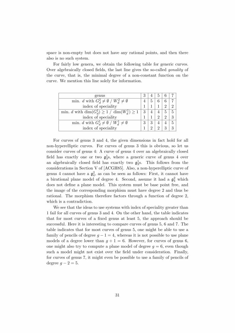
For fairly low genera, we obtain the following table for generic curves.

Over algebraically closed fields, the last line gives the so-called gonality of

the curve, that is, the minimal degree of a non-constant function on the

curve. We mention this line solely for information.

genus 3 4 5 6 7

min. d with G2d 6= ∅ / W 2

d 6= ∅ 4 5 6 6 7index of speciality 1 1 1 2 2

min. d with dim(G1d) ≥ 1 / dim(W 1

d ) ≥ 1 3 4 4 5 5index of speciality 1 1 2 2 3

min. d with G1d 6= ∅ / W 1

d 6= ∅ 3 3 4 4 5index of speciality 1 2 2 3 3

For curves of genus 3 and 4, the given dimensions in fact hold for all

non-hyperelliptic curves. For curves of genus 3 this is obvious, so let us

consider curves of genus 4: A curve of genus 4 over an algebraically closed

field has exactly one or two g13s, where a generic curve of genus 4 over

an algebraically closed field has exactly two g13s. This follows from the

considerations in Section V of [ACGH85]. Also, a non-hyperelliptic curve of

genus 4 cannot have a g24, as can be seen as follows: First, it cannot have

a birational plane model of degree 4. Second, assume it had a g24 which

does not define a plane model. This system must be base point free, and

the image of the corresponding morphism must have degree 2 and thus be

rational. The morphism therefore factors through a function of degree 2,

which is a contradiction.

We see that the ideas to use systems with index of speciality greater than

1 fail for all curves of genus 3 and 4. On the other hand, the table indicates

that for most curves of a fixed genus at least 5, the approach should be

successful. Here it is interesting to compare curves of genus 5, 6 and 7. The

table indicates that for most curves of genus 5, one might be able to use a

family of pencils of degree g − 1 = 4, whereas it is not possible to use plane

models of a degree lower than g + 1 = 6. However, for curves of genus 6,

one might also try to compute a plane model of degree g = 6, even though

such a model might not exist over the field under consideration. Finally,

for curves of genus 7, it might even be possible to use a family of pencils of

degree g − 2 = 5.

31

4.2 Computation of linear systems

We now give algorithms to compute special divisors (and thus special linear

systems) and discuss their application to the algorithm schemes given in the

previous section. Because of general interest into the subject, we discuss the

task to compute special linear systems a bit more generally than is necessary

for our applications.

As in Section 2 for the following geometric considerations, the ground

field is arbitrary. For algorithmic applications, we always restrict ourselves

to curves of a fixed genus over finite fields and to systems of a fixed degree.

4.2.1 A basic method

For reference, we discuss here what might be called the “basic method” to

compute complete special linear systems.

Let first C be a curve of genus g over any field k, and let ω be the canonical

sheaf on C. We start with the trivial observation that if D is a special divisor

then the system |ω(−D)| is by definition non-empty. Conversely, if D is any

effective divisor on C of degree d at most g − 1, the complete linear system

|ω(−D)| has degree 2g − 2− d and dimension g − 1− d+ dim(|D|) ≥ 0. Its

index of speciality is 1 + dim(|D|) ≥ 1. Moreover, the system |ω(−D)| only

depends on the complete linear system defined by D.

One can interpret this from a geometric point of view: For any natural

number d at most g−1 have an isomorphism between Cd and C12g−2−d which

is given by |D| 7→ |ω(−D)| on rational points (and likewise after any base

change to a field extension).

This gives a straightforward method to compute complete special linear

systems of a given degree d at least g − 1: One chooses an effective divisor

D of degree 2g − 2 − d and considers the system |ω(−D)|. We note here

that as shown in [Die11] one can compute a uniformly randomly computed

divisor of a given degree in polynomial time. However, this computation

relies on the computation of the L-polynomial of the curve which is possible

in polynomial time because we consider curves of a fixed genus but is not

practical at all for curves of genus 4 or higher, say.

The variant of the method to compute plane models mentioned in sub-

section 3.6.2 is based on systems of degree g + 1 computed like discussed

here. This idea was already discussed in [Die06].

4.2.2 A general method

We now go into the opposite direction and give a general method to compute

special divisors of a given degree and a given lower bound on the dimension.

More precisely, we give a method to compute such divisors which split com-

32

pletely into distinct rational points. The method is based on the techniques

introduced by Brill and Noether to study special linear systems.

We first give the essential theoretical observations we need. Let for this

any smooth proper curve C of genus g ≥ 3 over a field k be given, and let D

be an effective divisor of degree d on C. Then the Riemann-Roch Theorem

states that

dim(|D|) = dim(Γ(C, ω(−D))) + d− g .

We have the short exact sequence

0 −→ ω(−D) −→ ω −→ ω/ω(−D) −→ 0

We have the exact sequence

0 −→ Γ(C, ω(−D)) −→ Γ(C, ω) −→ Γ(C, ω/ω(−D)) .

Let n be the dimension of the image of Γ(C, ω) in Γ(C, ω/ω(−D)). Then by

Riemann-Roch

dim(|D|) = d− n .

We make this more explicit now. Let ω1, . . . , ωg be a basis of Γ(C, ω) and

letD = P1+· · ·+Pd with distinct k-rational points Pi. Then Γ(C, ω/ω(−D)) =⊕di=1 κ(Pi) and κ(Pi) = ωPi/(mPiωPi), which is a 1-dimensional k-vector

space. Now n is the rank of the matrix ((ωi(Pj)))i,j , whose entries in the

jth column lie in κ(Pj). Explicitly, we can fix one non-trivial differential ω,

express every ωj in the form ωj = fj · ω for a function fj and consider the

rank of the matrix ((fi(Pj)))i,j . This matrix is called Brill-Noether matrix

by Griffiths and Harris in [GH80]. Note that with K := div(ω), we have an

isomorphism L(K) −→ Γ(C, ω) , f 7→ f · ω.

Let now d and r be given. Then |D| has dimension at least r if and only

if the rank of the matrix is ≤ d − r. This means that the determinants of

all minors of size d− r + 1 of the matrix vanish.

So very briefly, we have the following method to compute such linear

systems: We first compute an effective canonical divisor K and a basis

f1, . . . , fg of L(K). Then we regard the Pi as unknown points on the curve

and express the condition that the determinants of all minors of size d−r+1

vanish by a non-linear system of equations in the coordinates of the Pi.

Note also that if D = P1 + · · ·+ Pd is one solution, then so is any effec-

tive divisor which is linearly equivalent to D and which splits into distinct

rational points. Because of this it is reasonable to fix ρ + r of the points,

where ρ is the Brill-Noether number defined above.

Concerning the systems of equations, there are in fact two obvious vari-

ants here: The first variant is that one starts off with a plane model. In this

case, obviously one only has one curve equation for each point Pi but the

33

determinants of the matrices are rather complicated. A second variant is to

consider the canonical embedding of the curve. In this case, each point has g

coordinates, and one has various equations for each point, but the functions

f1, . . . , fg are now just the coordinates x1, . . . , xg and the determinants are

as easy as possible.

In any case, for a fixed genus, degree and dimension, the number of vari-

ables and the number of equations is fixed and the degrees of the equations

are bounded. It is therefore reasonable to expect that the computation can

be performed in expected polynomial time. With a suitable variant of the

algorithm it should be possible to prove this.

Note that as discussed in the previous subsection, for any curve of genus

g and for d = dg2 + 32e the space W 1

d has dimension at least 1. One can now

apply the general algorithm given in subsection 3.5 to this family and access

the family as described. We note again that we have the two obvious ways

to represent the curve here: via a plane model or via a canonical curve.

On the basis of the heuristic assumptions discussed in subsection 3.5, one

obtains an algorithm to compute discrete logarithms for nearly all curves of

a fixed genus g with an expected running time of

O(q2− 2

d g+12 e).

This is the “Heuristic Result” given in the introduction.

The indicated index calculus algorithm seems however to be of little

practical value. Indeed, it seems to be very difficult to perform any practi-

cal and non-trivial computation with the indicated method to find special

divisors.

4.2.3 Pencils of degree g − 1

We have already seen that for a generic curve of genus g ≥ 3 the spaces

W 1g−1 and G1

g−1 have dimension g − 4, and for any curve the dimensions

are at least g − 4. By Marten’s theorem ([ACGH85, IV, §5]), for any non-

hyperelliptic curve the space W 1g−1 is g − 4-dimensional. We now discuss

a very efficient and easy method to compute pencils of degree g − 1 on

curves of genus at least 4. This leads to the practical algorithm to compute

discrete logarithms for curves of a fixed genus at least 5 mentioned in the

introduction. The following considerations are similar to the ones in Chapter

VI, §4 of [ACGH85].

a) Geometric considerations The basic idea of the method is as follows:

For every effective divisor A of degree g − 3 on C we consider all divisors

E of degree 2 with dim(|A + E|) ≥ 1. Clearly, in this way we obtain all

34

effective divisors of degree g − 1 on C of dimension at least 1 which split

into an effective divisor of degree g − 3 and an effective divisor of degree 2.

For our index calculus method the splitting of the divisor is no restriction

as we anyway only want to consider linear systems which contain at least

one completely split divisor.

Another observation is that for any divisor D of degree g − 1 on C one

has dim(|D|) = dim(|ω(−D)|).Let now A be an effective divisor on C of degree g−3. We show how one

can obtain all divisors E as indicated. For this we consider the complete

linear system |ω(−A)| of degree g + 1. The goal is to obtain all effective

divisors of degree 2 with dim(|ω(−A − E)|) = dim(|ω(−A)|(−E)) ≥ 1. We

make a case distinction.

1. Let us first assume that |ω(−A)| is base-point free of dimension 2. It thus

defines a morphism ϕ to P2k. (For the moment, the morphism need not

be birational onto its image, but as stated in Proposition 7 for a generic

divisor on a generic curve, this is the case.) For an effective divisor E

of degree 2, the divisors in |ω(−A)|(−E) are the divisors of the form

ϕ−1(L), where L is a line in P2k and E is a subdivisor of ϕ−1(L). We

discuss this now in detail: First, if the (set-theoretic) image of E does

not consist of exactly one rational point, there is only one such line: the

line through the image of E. Secondly, if the (set-theoretic) image of E is

a rational point P and if |ω(−A)|(−E) is a pencil then it is given by the

composition of ϕ with the central projection at P . With other words, we

have a pencil if and only if for every line L through P , E is a subdivisor

of ϕ−1(L). This is equivalent to E ≤ ϕ−1(P ).

We now study the important case that ϕ is birational onto its image.

In this case all E which define a pencil are subdivisors of a divisor of

the form ϕ−1(P ) for a singular point P . In the important special case

that all singular rational points of ϕ(C) are double points, the divisors E

which define a pencil are exactly the divisors defining the singularities.

In general, the divisor ϕ−1(P ) − E is then the base locus of the linear

system |ω(−A− E)|.

2. Let us now assume that |ω(−A)| is of dimension larger than 2. Then for

any effective divisor E of degree 2, |ω(−A−E)| is of dimension at least 1.

3. Finally let us now assume that |ω(−A)| is not base-point free and of di-

mension 2. Let B be the base locus, such that |ω(−A)| =

|ω(−A − B)| + B and |ω(−A − B)| is base point free of dimension 2.

Let again ϕ be an associated morphism to P2k, and let E be an effective

divisor of degree 2. Let us first assume that E and B are disjoint. Then

just as in the first case, |ω(−A−E)| is a pencil if and only if E is mapped

35

to a singular point of P2k and E ≤ ϕ−1(P ). On the other hand, if B and

E are not disjoint, there are the following cases: If B and E share exactly

one rational point, |ω(−A−E)| is a pencil and if E is a subdivisor of B

then |ω(−A− E)| has dimension 2.

b) The method The above points immediately lead to a method to com-

pute linear systems of degree g−1 and dimension at least 1 (usually pencils):

Let a curve C over a finite field k be given. One fixes an arbitrary effective

divisor A of degree g−3 and computes the linear system |ω(−A)|, that is one

computes K −A, where K is a canonical divisor, and a basis of L(K −D).

Let us assume that we are in the “generic case”, that is, the system is base-

point free and of dimension 2, and let f0, f1, f2 be the computed basis. (In

the other cases, following the outline above, the computation is even easier

than the following one.) Let ϕ be the morphism given by f0, f1, f2. One

computes a defining homogeneous equation of ϕ(C). Again we assume that

we are in the “generic case”, that is, ϕ(C) is a plane model, which then

has degree g + 1. As by assumption g ≥ 4, the arithmetic genus is g(g−1)2

which is always larger than g. So, it has singularities. One computes the

singular locus S with a Grobner base computation. If the locus does not

contain a rational point, one restarts the computation. Otherwise one fixes

one singular point, say S.

The task is now to compute ϕ−1(S). For this, one can proceed as follows:

One fixes two linear forms G1, G2 in k[X,Y, Z] defining lines through S

and considers the pencil given by the sheaf ω(−A) and the linear subspace

〈G1(f0, f1, f2), G2(f0, f1, f2)〉 of Γ(C, ω(−A)) = L(K − A). The base locus

of this pencil is exactly ϕ−1(S).

After ϕ−1(S) can been computed, one searches for a subdivisor E of

degree 2 of ϕ−1(S). Finally, one computes A+ E.

c) A Question It arises the following question. What is the probability

that the method succeeds provided that the effective divisor A is chosen

uniformly at random?

For a heuristic analysis it is reasonable to compare the singular locus

with a random polynomial of the same degree. Now, for polynomials of a

fixed degree n over finite fields Fq, the probability that such a polynomial

has a rational root is asymptotically equal to∑n

i=1(−1)i+1

i! . This can be

seen with the inclusion-exclusion principle. Explicitly, for n ≥ 4, this is in

between 0.625 and 0.634.

We studied the question experimentally: For each of the genera 5,6,7 we

performed the following experiments: We considered 10 prime fields with

cardinality between 219 to 230. Over each of the fields, we generated 10

36

curves with the Magma command RandomCurveByGenus. (The algorithm

for this command is also based on Brill-Noether theory; see [ST02].) On

each of the 10 curves per genus we generated 100 random prime divisors A

of degree g − 3. We observed the following:

The complete linear system |K−A| always defined a plane model (which

is then of degree g + 1).

In the following table, we give the range of the percentages of divisors

A on any of the curves which lead to a plane model with a rational singular

point. Additionally, we give the overall percentage of divisors A which lead

to a plane model with a rational singular point.

genus 5 6 7

percentage (range; average) 53 – 75; 64 52 – 74; 63 54 – 75; 62

The average values are close to the heuristically predicted value of about

63% for all genera.

On all the plane models, all singularities were double points. As to be

expected, all pencils contained at least one divisor which split into distinct

rational points. By Proposition 1 the number of divisors in a pencil d which

split completely into rational points is then & 1(g−1)!q.

d) Index calculus Concerning index calculus, there are two different ap-

proaches based on this method to compute pencils:

The first method is immediately given by the description to compute

elements of W 1g+1 described above: After a pencil has been computed, the

corresponding base point free linear system is used for relation generation

as indicated in the previous section. Following subsection 2.3 we call this

approach the implicit approach because the original plane model is always

kept. Or to put it differently, one does use different plane models to deter-

mine pencils, but after that one continues with the original plane model.

We note that the efficiency depends of course on the complexity of the

plane model one represents C with. So it is advisable to choose a plane

model of degree g + 1.

The second method is based on the explicit approach mentioned in sub-

section 2.3. Here, instead of the pencils |A + E| considered in the first

method, one uses the pencils |ω(−A−ϕ−1(S))|, where S is a singular point

of one of the plane models of degree g+1. Let us note here that the residual

system to |A + E|, |ω(−A − E)|, is also a pencil of degree g − 1, and the

pencil |ω(−A− ϕ−1(S))| is the corresponding base point free pencil.

Here one changes the plane model with each new divisor A. After one

has changed the model, one also maps the factor base to the new model.

37

The original model is also kept, because one needs it for the large primes

(rational points which do not lie in the factor base). The relation generation

in the new model is now very easy because it is based on the intersection of

a lines with the plane model, which is a very easy and fast computation. For

simplicity, one might only consider relations obtained from lines which do not

go through any other than the given singularity. However, if one has found

a relation containing large primes (that is, rational points not contained in

the factor base), one has to find the corresponding large primes. For this,

one has to map the points back to the original model.

Now, the task to map from the original plane model to the one given

by |ω(−D)| and the task to map back to the original plane model are very

similar. One just has to find the functions which define the original plane

model in terms of the new one.

The curve C is itself given by a plane model. As specified in the introduc-

tion, let π : C −→ P2k = Proj(k[X,Y, Z]) be the corresponding morphism.

We are really interested in the morphism π ◦ ϕ−1. The morphism π ◦ ϕ−1is given by (x|C ◦ ϕ−1, y|C ◦ ϕ−1, 1). We thus need to compute the functions

x|C ◦ ϕ−1 and y|C ◦ ϕ−1. Let us focus on the first of these functions. It is

determined by its value at one k-rational point and its principal divisor on

the normalization of ϕ(C). Provided that the image of the principal divisor

(x|C) is contained in the non-singular part of ϕ(C), this divisor is the image

of the principal divisor (x|C)) under ϕ.

So, we need to determine the image of the divisor (x|C) under ϕ. For

this, we first compute the divisor in free representation, that is, we factor

the divisor completely. For each closed point (prime divisor) in the divisor

we pass to a field extension λ|k such that the point splits completely into

rational points. We map such a point to ϕ(C)(λ). Let us assume that all

these points lie in the non-singular part of ϕ(C). Then we compute the

corresponding divisor in ideal representation and its Riemann-Roch space.

There is a certain possibility of failure here due to the fact that we

require that the image of the points lie in the non-singular part of ϕ(C). If

the procedure fails, we can apply a linear coordinate transformation. Like

this, one can compute the birational inverse of ϕ in polynomial expected

time.

4.2.4 Plane models of curves of genus 6

By Brill-Noether theory a generic curve of genus 6 over an algebraically

closed field has a birational plane model of degree 6. Indeed, for generic

curve, the spacesG26 andW 2

6 are equal, zero-dimensional and reduced. More-

over, by [ACGH85, V, Theorem 1.3] they have exactly 5 geometric points.

38

A curve over a finite field might not have such a model, even if such a

model exists over an extension field. Heuristically, for q −→ ∞ the prob-

ability that an isomorphism class of a curve over Fq has such a model is

asymptotically equal to the probability that a polynomial of degree 5 has a

root over Fq, and as already mentioned this probability is about 63%.

In principle, to compute a complete linear system of degree 6 and di-

mension 2 one might use the general approach via Brill-Noether matrices.

However, as already indicated, this computation is not practical at all. We

note that by Riemann-Roch one might also compute a complete linear sys-

tem of degree 4 and dimension 1. But this is by itself of no help either.

However, there is a method which is efficient from a practical point of

view due to F.-O. Schreyer ([Sch86]). This method was revisited by M.

Harrison and has been implemented by him in the computer algebra system

Magma ([Har13], [BCFS11]). We performed experiments with the method

which confirmed the heuristic estimate that about 63% of all curves of genus

6 over finite fields have a plane model of degree 6.

Sometimes there also exists a birational plane model of degree 5 for a

curve of genus 6, namely when the curve C is isomorphic to a smooth plane

quintic. If this is the case the corresponding g25 is unique, therefore fixed

under the action of Gal(k/k) and hence a k-rational point of G25. The plane

quintic can be found by an algorithm described in [Har13]. However, Harri-

son’s algorithm has some trouble dealing with a base field of characteristic 3.

The g25 on C leads to a 1-dimensional family of pencils of degree 4 by

central projection. Interestingly, in this case one can also use the method

presented in subsection 4.2.3 b) to compute such pencils::

By the discussion in [ACGH85, V] following Theorem 1.1 therein every

complete g15 on Ck is given as |N − P1 + P2| for N in the unique g25 on Ck,P1, P2 ∈ C(k), P1 6= P2, and hence possesses a base point P2. Furthermore,

there are no pencils of degree 2 or 3 on a non-singular plane quintic because

the curve is neither hyperelliptic nor possesses pencils of degree 3 by [GH78,

p. 535].

Thus if the result of the computation is a complete g15, one can subtract

the base point (which is then k-rational) to obtain a g14. In case the result

of the computation is an incomplete g15, the corresponding complete system

is the unique g25, which one now has computed. Furthermore, as every g15which contains a completely split divisor can be generated as described in

subsection 4.2.3 a), b), so can now every g14.

These considerations also have an interesting interpretation for birational

plane models of degree g + 1 = 7: The fact that every g15 has a base point

implies now that every singularity of a plane model of degree 7 is of degree 3.

39

4.3 Experiments

In the previous subsection 4.2 we presented four methods to compute special

linear systems. The “general method” given in subsection 4.2.2 relies on the

use of the Brill-Noether matrix and leads to the “Heuristic Result” stated

in the introduction; as mentioned before it is of little practical value. This

is because the resulting systems of polynomial equations cannot be solved

in an appropriate time. So for the following experiments we will focus on

the methods using pencils of degree g − 1 presented in subsection 4.2.3.

4.3.1 Setup

We intend to show that an algorithm based on pencils of small degree is in-

deed practical. Hence we implemented the algorithm relying on the explicit

approach described in subsection 4.2.3. This method was referred to the im-

plicit approach because the intersection of different plane models with lines

can be calculated very fast. We will refer to the corresponding algorithm as

the new algorithm.

We are especially interested in a comparison to the algorithm which is

introduced in [Die06] and which we will call the old algorithm. We recall

that in [Die06] it is argued that one can solve the discrete logarithm problem

for curves of a fixed genus g ≥ 2 in an expected time of

O(q2− 2

g−1 ) .

The corresponding algorithm, which is recalled in subsection 3.6.2, works

with one plane model of degree g + 1 and intersecting randomly chosen

lines with this plane model. A function based on this approach is already

available in Magma under the name IndexCalculus. Nevertheless, we also

implemented a new version of this algorithm in order to be able to vary

different parameters like the size of the matrix of relations and the number

of vertices in the graph of large prime relations.

On the other hand above we argued that the new algorithm solves the

discrete logarithm problem for nearly all curves of a fixed genus g ≥ 5 in an

expected time of

O(q2− 2

g−2 ) .

We now briefly describe the specifications made for both algorithms.

The old algorithm proceeds in three steps. Given a plane model of C and

two divisor classes in Cl0(C), in a first step we apply the method described

in [Die06] to generate q FP- or PP-relations. From this we build the graph

G of large prime relations using a factor base F of size k := dκ · q1−1

g−1 ewhere κ := (4 · (g − 1)!)

1g−1 is chosen as indicated in [Die06]. So for g = 4, 5

40

κ is approximately 2.8 and 3.1, respectively. We note that, as argued in

subsection 3.5, asymptotically any κ larger than (2 · (g − 1)!)1

g−1 should be

sufficient. In a second step we use a breadth-first search to construct a short-

est path tree T on the graph. We then create further relations factoring over

F∪V, where V is the vertex set of T . In contrast to the description following

Proposition 2, these relations are generated in the same way as before, that

is, also by intersecting the plane model with lines. Whenever an appropri-

ate relation is created, we check if it has already been constructed before.

This can easily be done using the aggregate ”set” in Magma. Substituting

elements of V with the help of T we generate a matrix of relations R with

slightly more rows than columns. Then we apply the Lanczos algorithm to

find a non-trivial row vector γ in the left kernel of R.

The new algorithm on the other hand starts with the same input and a

factor base F of size dκ·q1−1

g−2 e. We want the running times for the relation

generation and the linear algebra step to be similar so experimentally we

decided to set κ := 1. As argued in subsection 3.5 one cannot guarantee

that there are lines in P2Fq

factoring over F for any plane model of C. So we

increase F by up to g − 3 new elements for each of the plane models used.

Again, we always check if a relation has already been constructed. Fur-

thermore, in order to decrease the number of duplicates during the relation

generation process, for each pencil |ω(−A−ϕ−1(P ))| given by a singularity

P of a plane model defined by |ω(−A)|, we only consider lines through P and

ϕ(Q) where Q ∈ {P1, . . . , Pd k2e} with F = {P1, . . . , Pk}. As before we create

a graph G with q vertices in this way and consider the tree T constructed

from G by breadth-first search.

Just as in the case of the old algorithm we use the identical relation

generation method as in the construction of G to generate a matrix of re-

lations R′ from T . Again we stop the construction of R′ if it has slightly

more columns than rows. As before we solve the corresponding system of

equations by applying the Lanczos algorithm.

We intend to compare the old algorithm for genus 4 or 5 to the new algo-

rithm for genus 5 or 6, respectively. For this we generated curves of the de-

sired genera over F3, F5 and F7 by the Magma function RandomCurveByGenus

and made a base change to the fields used in the tables below. We had to

proceed this way so we could calculate the order N of the degree-zero class

groups using the L-polynomial. We then picked the biggest prime ` in the

factorization of N and generated a random divisor class a of degree 0 on the

corresponding curve which had order `. We set b := n · a where the integer

n was chosen from {1, . . . , ` − 1} uniformly at random and computed the

discrete logarithm of b with respect to a using the new or the old algorithm.

41

4.3.2 Results

The results for varying fields can be found in the tables below where Trel and

Tla stand for the time (in seconds) needed to create R and solving γR = 0,

respectively.

F57 = F78125 genus size of F Trel Tla

old algorithm 4 5271 1039 691

new algorithm 5 5133 2018 1473

old algorithm 5 14627 7333 11683

new algorithm 6 14424 18782 21959

F311 = F177147 genus size of F Trel Tla

old algorithm 4 9098 3532 4395

new algorithm 5 8795 7233 7419

old algorithm 5 27028 27799 45041

new algorithm 6 26394 75352 83735

F77 = F823543 genus size of F Trel Tla

old algorithm 4 25343 29519 38227

new algorithm 5 24445 41676 63201

F313 = F1594323 genus size of F Trel Tla

old algorithm 4 39366 183060 152127

new algorithm 5 37830 258485 283730

The arguments in subsection 4.2.2 as well as the heuristic result in [Die06]

indicate that, at least for q → ∞, applying the new algorithms instead of

the old one means dropping the genus by one. The experiments show that

this also holds from a practical point of view: the running times of the new

algorithm for genus g = 5, 6 differ from those of the old algorithm for genus

g−1 only by a factor between 1.5 and 2.0 for g = 5 and between 1.7 and 1.9

for g = 6. This difference comes from the way relations are generated. The

old algorithm only uses one plane model whereas the new algorithm varies

the plane model and maps the factor base and large primes back and forth

between these models.

Changing the plane model various times also has an effect on F . During

the new algorithm the original factor base of size dq1−1

g−2 e is increased by

a factor of about 2.8 for g = 5 and 3.1 for g = 6. This also indicates

42

why we did not choose κ considerably smaller than 1, because this meant

a bigger increase of F in each step. So the advantage of a smaller factor

base at the beginning would be almost canceled during the process of relation

generation. A bigger constant on the other hand would mean bigger matrices

and hence the Lanczos algorithm would take considerably longer. It is also

worth noting that the factor by which F is increased is the same that we

chose for κ in the old algorithm if the genus is dropped by one. So the

sizes of the sparse matrices R′ generated by the new algorithm are similar

to those of the corresponding matrices R created by the old algorithm.

On the other hand, we observed that matrices of type R′ had 3.1 to

3.5 times the density of matrices of type R for which the genus is dropped

by one. This can be explained by the more complicated way relations are

generated in the new algorithm.

4.3.3 Further Observations

We note that the testing we did was primarily designed to check the behavior

of the new algorithm in comparison to the old one. In particular we intended

to show that the relation generation via different plane models and lines

through singular points is practical. So far this could only be tested in full

for curves which are generated by base change. Nevertheless we also did

some testing of the relation generation step for fields of bigger characteristic

as well and the corresponding results did not differ significantly from the

ones above.

As expected for q sufficiently large and g = 5, 6 in the considered cases

the new algorithm never failed. So first of all there always existed enough

linear systems |ω(−A − ϕ−1(P ))| ∈ W rd to create the graph of large prime

relations as indicated by Brill-Noether theory. Secondly, the relations gen-

erated by different plane models in the way described above are sufficiently

independent. However, in order to get matrices of appropriate rank we had

to create them from slightly more relations than factor base elements. In

fact, the Lanczos algorithm almost always succeeded with matrices of size

(#F + 10)×#F . There is the rare possibility that a curve C of genus 5

possesses a g13. Following the discussion in [ACGH85, V] after Theorem 1.1

we see that in this case the g13 is unique. Experimentally we rediscovered

this g13 in every plane model of C by finding a singularity of multiplicity 3.

In this case we got linearly dependent relations more often and hence had

to generate more relations than usual. The old algorithm did not succeed

with matrices of this size in some more cases. Twice we had to consider

considerably more relations. The reason for this necessary adjustment is

unclear to us.

43

The main difficulties while implementing the new algorithm were caused

by the linear algebra step. The function ModularSolution specified for in-

dex calculus and relying on either structured Gaussian elimination or the

Lanczos algorithm is available in Magma but failed to work reliably for large

finite fields. The Gaussian elimination got extremely slow whenever the

group order was prime, and often ModularSolution did not succeed indepen-

dently from the chosen option. So we implemented the Lanczos algorithm

based on [LO91] ourselves in Magma and in the C++ library LinBox. It

turned out that Magma was about twice as fast multiplying dense vectors

by sparse matrices and hence our implementation in Magma is considerably

faster than our implementation in LinBox. So in order to get the results

above we chose to use our Magma version of the Lanczos algorithm.

We also encountered failures in Magma in some other cases. Whenever

there is a considerably large set of tuples initiated, ”for” loops are executed

more slowly depending on the set’s size. However, when the set only consists

of field elements or elements in an affine or projective space this was not the

case. Hence we adjusted the implementation so that only sets of the above

form are used to save the generated relations. Furthermore we got an error

whenever we tried to check if a given divisor on a plane curve is principal. On

the other hand a similar function worked fine for divisors of function fields.

So in contrast to the Magma function IndexCalculus we decided to represent

the input curve by the function field of a corresponding plane model and

not by the plane model itself. Finally, in certain cases, we had to delete the

vertex set of a given graph before ending the function as otherwise we got

an internal error.

References

[ACGH85] E. Arbarello, M. Cornalba, P. Griffiths, and J. Harris. Geometry

of Algebraic Curves. Springer-Verlag, 1985.

[BCFS11] W. Bosma, J. Cannon, C. Fieker, and A. Steel, editors. Handbook

of Magma functions, Edition 2.17. 2011.

[Die06] C. Diem. An Index Calculus Algorithm for Plane Curves of Small

Degree. In F. Hess, S. Pauli, and M. Pohst, editors, Algorithmic

Number Theory — ANTS VII, LNCS 4076, pages 543 – 557,

Berlin, 2006. Springer.

[Die11] C. Diem. On the discrete logarithm problem in class groups of

curves. Math.Comp., 80:443 – 475, 2011.

[Die12a] C. Diem. On the discrete logarithm problem for plane curves.

Journal de Theorie des Nombres de Bordeaux, 24:639–667, 2012.

44

[Die12b] C. Diem. On the use of expansion series for stream ciphers. LMS

J. Comput. Math., 15:326–340, 2012.

[DT08] C. Diem and E. Thome. Index calculus in class groups of non-

hyperelliptic curves of genus three. J. Cryptology, 21:593–611,

2008.

[EG02] A. Enge and P. Gaudry. A general framework for subexponential

discrete logarithm algorithms. Acta. Arith., 102:83–103, 2002.

[FL81] W. Fulton and R. Lazarsfeld. On the connectedness of degener-

acy loci and special divisors. Acta Math., 146:271–283, 1981.

[Gau00] P. Gaudry. An algorithm for solving the discrete log problem

on hyperelliptic curves. In Advances in Cryptology — EURO-

CRYPT 2000, LNCS 1807, pages 19–34. Springer-Verlag, 2000.

[GH78] P. Griffiths and J. Harris. Principals of algebraic geometry. Wiley

International, 1978.

[GH80] P. Griffiths and J. Harris. On the variety of special linear systems

on a general algebraic curve. Duke Math. J., 47(1):233–272, 1980.

[Gie82] D. Gieseker. Stable curves and special divisors: Petri’s conjec-

ture. Invent. Math., 66:251–275, 1982.

[Gro] A. Grothendieck with J. Dieudonne. Elements de Geometrie

Algebrique (I-IV). ch. I: Springer-Verlag, Berlin, 1971; ch. II-

IV: Publ. Math. Inst. Hautes Etud. Sci. 8,11, 17, 20,24, 28, 32,

1961-68.

[GTTD07] P. Gaudry, E. Thome, N. Theriault, and C. Diem. A double

large prime variation for small genus hyperelliptic index calculus.

Math. Comp., 76:475–492, 2007.

[Har13] M. Harrison. Explicit solution by radicals, gonal maps and plane

models of algebraic curves of genus 5 or 6. J. Symb. Comput.,

pages 3–21, 2013.

[Heß01] F. Heß. Computing Riemann-Roch spaces in algebraic function

fields and related topics. J. Symb. Comput., 11, 2001.

[Heß05] F. Heß. Computing relations in divisor class groups of algebraic

curves over finite fields. preprint, ca. 2005.

[KL72] S. Kleiman and D. Laksov. On the existence of special divisors.

Amer. J. Math., 94:431–436, 1972.

45

[KL74] S. Kleiman and D. Laksov. Another proof of the existence of

special divisors. Acta Math., 132:163–176, 1974.

[LO91] B. A. LaMacchia and A. M. Odlyzko. Solving large sparse linear

systems over finite fields. In Proceedings of the 10th Annual

International Cryptology Conference on Advances in Cryptol-

ogy, CRYPTO ’90, pages 109–133, London, UK, 1991. Springer-

Verlag.

[Mil98] J. Milne. Jacobian Varieties. In G. Cornell and J. Silverman,

editors, Arithemtic Geometry, pages 167–212. Springer-Verlag,

1998.

[MS94] V.K. Murty and J. Scherk. Effective versions of the Chebotarev

density theorem for funciton fields. C. R. Acad. Sci., 319:523–

528, 1994.

[Nag07] K. Nagao. Index calculus attack for Jacobian of hyperelliptic

curves of small genus using two large primes. Japan J. Indust.

Appl. Math., 24, 2007.

[PH78] S. Pohlig and M. Hellnan. An Improved Algorithm for Comput-

ing Logarithms over GF(p) and its Cryptographic Significance.

IEEE Transactions on Information Theory, 1978.

[Pil90] J. Pila. Frobenius maps of abelian varieties and fining roots of

unity in finite fields. Math. Comp., 55:745–763, 1990.

[Pil91] J. Pila. Counting points on curves over families in polynomial

time. Available on the arXiv under math.NT/0504570, 1991.

[Sch86] F.-O. Schreyer. Syzygies of canonical curves and special linear

series. Math. Ann., 275, 1986.

[ST02] F.-O. Schreyer and F. Tonoli. Needles in a Haystack: Special

Varieties via Small Fields. In Eisenbud et al, editor, Computa-

tions in Algebraic Geometry with Macaulay 2, pages 215 – 277.

Springer Verlag, 2002.

[The03] N. Theriault. Index calculus attack for hyperelliptic curves of

small genus. In Advances in Cryptology — ASIACRYPT 2003,

volume 2894 of LNCS, pages 75–92. Springer-Verlag, 2003.

46