Computer Aided Geometric Design 30 (2013) 827–843

Contents lists available at ScienceDirect

Computer Aided Geometric Design

www.elsevier.com/locate/cagd

Modified T-splines ✩

Hongmei Kang, Falai Chen ∗, Jiansong Deng

School of Mathematical Sciences, University of Science and Technology of China, Hefei 230026, PR China

a r t i c l e i n f o a b s t r a c t

Article history:Received 6 January 2013Received in revised form 13 June 2013Accepted 30 September 2013Available online 17 October 2013

Keywords:T-meshT-splineKnot deletionSurface fittingSurface simplification

T-splines are a generalization of NURBS surfaces, the control meshes of which allow T-junctions. T-splines can significantly reduce the number of superfluous control points inNURBS surfaces, and provide valuable operations such as local refinement and mergingof several B-splines surfaces in a consistent framework. In this paper, we propose avariant of T-splines called Modified T-splines. The basic idea is to construct a set of basisfunctions for a given T-mesh that have the following nice properties: non-negativity, linearindependence, partition of unity and compact support. Due to the good properties of thebasis functions, the Modified T-splines are favorable both in adaptive geometric modelingand isogeometric analysis.

© 2013 Elsevier B.V. All rights reserved.

1. Introduction

T-splines were introduced by Sederberg et al. (2003, 2004) and have been studied extensively in the last ten years.T-splines are a generalization of NURBS surfaces, the control meshes of which permit T-junctions. Unlike NURBS, T-junctionsallow T-splines to be locally refinable without propagating entire columns or rows. This property makes T-splines an idealtechnology for removing superfluous control points in NURBS surfaces and for adaptive isogeometric analysis (Hughes etal., 2005; Cottrell et al., 2009). Initial investigations using T-splines as a basis for isogeometric analysis demonstrate thatT-splines possess similar convergence properties as NURBS with far fewer degrees of freedom (Dörfel et al., 2009; Bazilevset al., 2010). However, the blending functions of T-splines are not always linearly independent. Buffa et al. (2010) gavean example of a T-spline with linearly dependent blending functions. This causes concerns about the linear independenceof T-splines. A solution to this problem is the so-called analysis-suitable T-splines (AST-splines for short) (Li et al., 2012;Scott et al., 2012). AST-splines are a subset of T-splines defined over a restricted T-mesh whose T-junction extensions donot intersect, and the blending functions are always linearly independent and thus are suitable for isogeometric analysis.However, the topology of the meshes of AST-splines is relatively restrict. For example, the mesh for common local refinementin isogeometric analysis as shown in Fig. 1 is not an AST-mesh. Algorithm exists for modifying a non-AST-mesh into anAST-mesh (Scott et al., 2012).

In Deng et al. (2008), the authors introduced the concept of splines over T-meshes, and specifically PHT-splines wereproposed. PHT-splines are polynomial splines defined over a hierarchical T-mesh, and the basis functions of PHT-splines arelinearly independent, form a partition of unity and have compact supports. The local refinement algorithm of PHT-splinesis local and very simple. Furthermore, since a PHT-spline is a polynomial (instead of a piecewise polynomial) over each cellof the T-mesh, it holds a good approximation property. These properties make PHT-splines an ideal tool for isogeometric

✩ This paper has been recommended for acceptance by B. Juettler.

* Corresponding author.E-mail address: chenfl@ustc.edu.cn (F. Chen).

0167-8396/$ – see front matter © 2013 Elsevier B.V. All rights reserved.http://dx.doi.org/10.1016/j.cagd.2013.09.001

828 H. Kang et al. / Computer Aided Geometric Design 30 (2013) 827–843

Fig. 1. A non-AST-mesh.

analysis (Nguyen-Thanh et al., 2011a, 2011b). However, PHT-splines are only C1 continuous, which is a disadvantage forgeometric modeling.

Another type of local refinement splines is LR-splines introduced by Dokken et al. (2013). LR-splines are defined on aμ-extended LR-mesh which is constructed by inserting line segments starting from a tensor product mesh according tocertain rules. LR-spline also forms a non-negative partition of unity and spans the complete piecewise polynomial space onthe mesh when the mesh construction follows certain rules. Different strategies can be employed to construct linearly inde-pendent LR B-splines by mesh modification. However, unlike T-splines and tensor product B-splines, there is no one-to-onecorrespondence between the 3D control mesh and the LR B-spline functions.

Hierarchical B-splines were introduced by Forsey and Bartels (1988), which have been recently further elaborated byGiannelli et al. (2012). The idea is to suitably truncate hierarchical B-spline functions according to finer levels in the hier-archy, which are called THB-splines. A THB-spline is a linear combination of B-splines, and THB-splines form a partition ofunity and are linearly independent.

In this paper, we introduce a new type of local refinement splines called Modified T-splines, which inherit some goodproperties of the above splines while preventing some undesirable properties. The intuitive idea is to construct a set of basisfunctions which have good properties, such as non-negativity, partition of unity, linear independence and compact support.With the help of an auxiliary T-mesh T ′ (defined in Lemma 3.2), the basis functions are constructed as a linear combinationof T-splines defined over T ′ . In this sense, Modified T-splines have some similarity with THB-splines.

The remainder of the current paper is organized as follows. In Section 2, we recall some preliminary knowledge aboutknot deletion of B-splines and T-splines. In Section 3, the construction details of Modified T-splines are described, and someproperties, especially approximation property of Modified T-splines are discussed. Section 4 demonstrates some applicationsof Modified T-splines in surface fitting. Section 5 concludes the paper with a summary and future work.

2. Preliminaries

In this section, we recall some preliminary knowledge about knot deletion of B-splines in one dimension which is usefulin the construction of Modified T-splines. Then the basic concepts about T-meshes and T-splines are reviewed.

2.1. Knot deletion of univariate B-splines

For simplicity, we only consider degree one and degree three B-splines for illustration.Given a knot vector t = [t0, t1, . . . , tn] with t0 � t1 � · · · � tn , the associated B-spline basis functions are defined recur-

sively as follows

N0i (t) =

{1, t ∈ [ti, ti+1),

0, otherwise,(1)

Nki (t) = t − ti

ti+k − tiNk−1

i (t) + ti+k+1 − t

ti+k+1 − ti+1Nk−1

i+1 (t), k � 1. (2)

We use N1[ti−1, ti, ti+1](t) to denote the degree one B-spline basis function N1i−1(t) and call it the linear B-spline basis

function at knot ti . Similarly, for cubic B-spline functions, N3[ti−2, ti−1, ti, ti+1, ti+2](t) = N3i−2(t) is called the cubic B-spline

basis function at knot ti .Now insert a knot t into the knot vector t to get a new knot vector t. Without loss of generality, we assume t ∈ [t3, t4).

Then the B-spline basis functions associated with t either can be written as a linear combination of the B-spline basisfunctions associated with t or remain unchanged. The relationship between these basis functions can be written as

H. Kang et al. / Computer Aided Geometric Design 30 (2013) 827–843 829

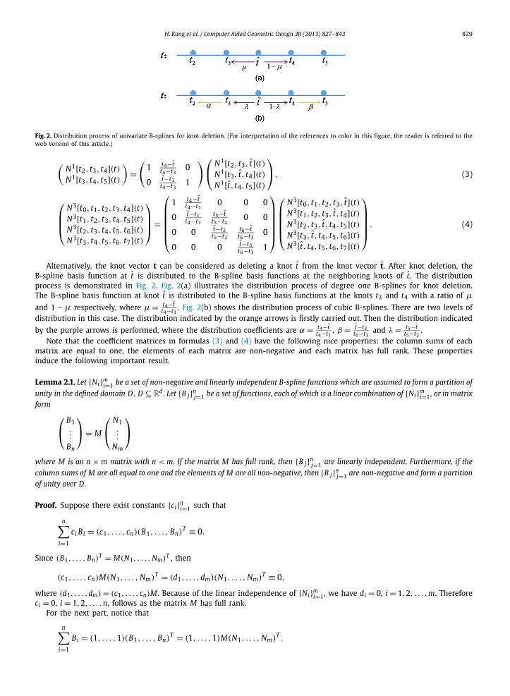
Fig. 2. Distribution process of univariate B-splines for knot deletion. (For interpretation of the references to color in this figure, the reader is referred to theweb version of this article.)

(N1[t2, t3, t4](t)N1[t3, t4, t5](t)

)=

(1 t4−t

t4−t30

0 t−t3t4−t3

1

)⎛⎝ N1[t2, t3, t](t)

N1[t3, t, t4](t)N1[t, t4, t5](t)

⎞⎠ , (3)

⎛⎜⎜⎝

N3[t0, t1, t2, t3, t4](t)N3[t1, t2, t3, t4, t5](t)N3[t2, t3, t4, t5, t6](t)N3[t3, t4, t5, t6, t7](t)

⎞⎟⎟⎠ =

⎛⎜⎜⎜⎜⎜⎝

1 t4−tt4−t1

0 0 0

0 t−t1t4−t1

t5−tt5−t2

0 0

0 0 t−t2t5−t2

t6−tt6−t3

0

0 0 0 t−t3t6−t3

1

⎞⎟⎟⎟⎟⎟⎠

⎛⎜⎜⎜⎜⎝

N3[t0, t1, t2, t3, t](t)N3[t1, t2, t3, t, t4](t)N3[t2, t3, t, t4, t5](t)N3[t3, t, t4, t5, t6](t)N3[t, t4, t5, t6, t7](t)

⎞⎟⎟⎟⎟⎠ . (4)

Alternatively, the knot vector t can be considered as deleting a knot t from the knot vector t. After knot deletion, theB-spline basis function at t is distributed to the B-spline basis functions at the neighboring knots of t . The distributionprocess is demonstrated in Fig. 2. Fig. 2(a) illustrates the distribution process of degree one B-splines for knot deletion.The B-spline basis function at knot t is distributed to the B-spline basis functions at the knots t3 and t4 with a ratio of μ

and 1 − μ respectively, where μ = t4−tt4−t3

. Fig. 2(b) shows the distribution process of cubic B-splines. There are two levels ofdistribution in this case. The distribution indicated by the orange arrows is firstly carried out. Then the distribution indicated

by the purple arrows is performed, where the distribution coefficients are α = t4−tt4−t1

, β = t−t3t6−t3

and λ = t5−tt5−t2

.Note that the coefficient matrices in formulas (3) and (4) have the following nice properties: the column sums of each

matrix are equal to one, the elements of each matrix are non-negative and each matrix has full rank. These propertiesinduce the following important result.

Lemma 2.1. Let {Ni}mi=1 be a set of non-negative and linearly independent B-spline functions which are assumed to form a partition of

unity in the defined domain D, D ⊆Rd. Let {B j}n

j=1 be a set of functions, each of which is a linear combination of {Ni}mi=1 , or in matrix

form ⎛⎝ B1

...

Bn

⎞⎠ = M

⎛⎝ N1

...

Nm

⎞⎠

where M is an n × m matrix with n < m. If the matrix M has full rank, then {B j}nj=1 are linearly independent. Furthermore, if the

column sums of M are all equal to one and the elements of M are all non-negative, then {B j}nj=1 are non-negative and form a partition

of unity over D.

Proof. Suppose there exist constants {ci}ni=1 such that

n∑i=1

ci Bi = (c1, . . . , cn)(B1, . . . , Bn)T ≡ 0.

Since (B1, . . . , Bn)T = M(N1, . . . , Nm)T , then

(c1, . . . , cn)M(N1, . . . , Nm)T = (d1, . . . ,dm)(N1, . . . , Nm)T ≡ 0,

where (d1, . . . ,dm) = (c1, . . . , cn)M . Because of the linear independence of {Ni}mi=1, we have di = 0, i = 1,2, . . . ,m. Therefore

ci = 0, i = 1,2, . . . ,n, follows as the matrix M has full rank.For the next part, notice that

n∑Bi = (1, . . . ,1)(B1, . . . , Bn)

T = (1, . . . ,1)M(N1, . . . , Nm)T .

i=1

830 H. Kang et al. / Computer Aided Geometric Design 30 (2013) 827–843

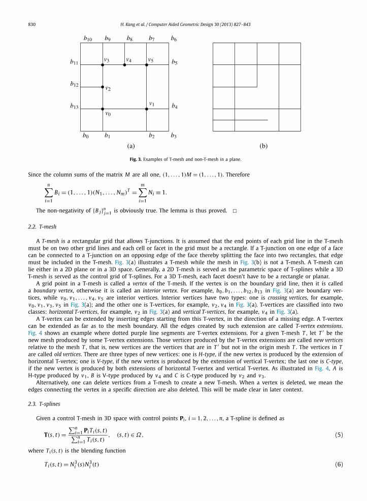
Fig. 3. Examples of T-mesh and non-T-mesh in a plane.

Since the column sums of the matrix M are all one, (1, . . . ,1)M = (1, . . . ,1). Therefore

n∑i=1

Bi = (1, . . . ,1)(N1, . . . , Nm)T =m∑

i=1

Ni ≡ 1.

The non-negativity of {B j}nj=1 is obviously true. The lemma is thus proved. �

2.2. T-mesh

A T-mesh is a rectangular grid that allows T-junctions. It is assumed that the end points of each grid line in the T-meshmust be on two other grid lines and each cell or facet in the grid must be a rectangle. If a T-junction on one edge of a facecan be connected to a T-junction on an opposing edge of the face thereby splitting the face into two rectangles, that edgemust be included in the T-mesh. Fig. 3(a) illustrates a T-mesh while the mesh in Fig. 3(b) is not a T-mesh. A T-mesh canlie either in a 2D plane or in a 3D space. Generally, a 2D T-mesh is served as the parametric space of T-splines while a 3DT-mesh is served as the control grid of T-splines. For a 3D T-mesh, each facet doesn’t have to be a rectangle or planar.

A grid point in a T-mesh is called a vertex of the T-mesh. If the vertex is on the boundary grid line, then it is calleda boundary vertex, otherwise it is called an interior vertex. For example, b0,b1, . . . ,b12,b13 in Fig. 3(a) are boundary ver-tices, while v0, v1, . . . , v4, v5 are interior vertices. Interior vertices have two types: one is crossing vertices, for example,v0, v1, v3, v5 in Fig. 3(a); and the other one is T-vertices, for example, v2, v4 in Fig. 3(a). T-vertices are classified into twoclasses: horizontal T-vertices, for example, v2 in Fig. 3(a) and vertical T-vertices, for example, v4 in Fig. 3(a).

A T-vertex can be extended by inserting edges starting from this T-vertex, in the direction of a missing edge. A T-vertexcan be extended as far as to the mesh boundary. All the edges created by such extension are called T-vertex extensions.Fig. 4 shows an example where dotted purple line segments are T-vertex extensions. For a given T-mesh T , let T ′ be thenew mesh produced by some T-vertex extensions. Those vertices produced by the T-vertex extensions are called new verticesrelative to the mesh T , that is, new vertices are the vertices that are in T ′ but not in the origin mesh T . The vertices in Tare called old vertices. There are three types of new vertices: one is H-type, if the new vertex is produced by the extension ofhorizontal T-vertex; one is V-type, if the new vertex is produced by the extension of vertical T-vertex; the last one is C-type,if the new vertex is produced by both extensions of horizontal T-vertex and vertical T-vertex. As illustrated in Fig. 4, A isH-type produced by v1, B is V-type produced by v4 and C is C-type produced by v2 and v3.

Alternatively, one can delete vertices from a T-mesh to create a new T-mesh. When a vertex is deleted, we mean theedges connecting the vertex in a specific direction are also deleted. This will be made clear in later context.

2.3. T-splines

Given a control T-mesh in 3D space with control points Pi , i = 1,2, . . . ,n, a T-spline is defined as

T(s, t) =∑n

i=1 Pi T i(s, t)∑ni=1 Ti(s, t)

, (s, t) ∈ Ω, (5)

where Ti(s, t) is the blending function

Ti(s, t) = N3(s)N3(t) (6)

i i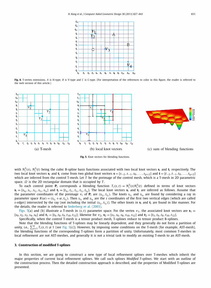

H. Kang et al. / Computer Aided Geometric Design 30 (2013) 827–843 831

Fig. 4. T-vertex extensions, A is H-type, B is V-type and C is C-type. (For interpretation of the references to color in this figure, the reader is referred tothe web version of this article.)

Fig. 5. Knot vectors for blending functions.

with N3i (s), N3

i (t) being the cubic B-spline basis functions associated with two local knot vectors si and ti respectively. Thetwo local knot vectors si and ti come from two global knot vectors s = [s−2, s−1, s0, . . . , sp+2] and t = [t−2, t−1, t0, . . . , tq+2]which are inferred from the control T-mesh. Let T be the preimage of the control mesh, which is a T-mesh in 2D parametricspace. Ω is the 2D rectangular domain that is occupied by T .

To each control point Pi corresponds a blending function Ti(s, t) = N3i (s)N3

i (t) defined in terms of knot vectorssi = [si0 , si1 , si2 , si3 , si4 ] and ti = [ti0 , ti1 , ti2 , ti3 , ti4 ]. The local knot vectors si and ti are inferred as follows. Assume thatthe parameter coordinates of the preimage vi of Pi are (si2 , ti2 ). The knots si3 and si4 are found by considering a ray inparameter space R(α) = (si2 + α, ti2 ). Then si3 and si4 are the s coordinates of the first two vertical edges (which are calleds-edges) intersected by the ray (not including the initial (si2 , ti2 )). The other knots in si and ti are found in like manner. Forthe details, the reader is referred to Sederberg et al. (2003).

Figs. 5(a) and (b) illustrate a T-mesh in (s, t) parameter space. For the vertex v1, the associated knot vectors are s1 =[s0, s2, s3, s4, s6] and t1 = [t6, t8, t9, t10, t12]; likewise for v2, s2 = [s5, s6, s8, s10, s12] and t2 = [t5, t6, t8, t10, t12].

Specifically, when the control T-mesh is a tensor product mesh, T-splines reduce to tensor product B-splines.Note that the blending functions of T-splines may be linearly dependent, and they generally do not form a partition of

unity, i.e.,∑n

i=1 Ti(s, t) �≡ 1 (see Fig. 5(c)). However, by imposing some conditions on the T-mesh (for example, AST-mesh),the blending functions of the corresponding T-splines form a partition of unity. Unfortunately, most common T-meshes inlocal refinement are not AST-meshes, and generally it is not a trivial task to modify an existing T-mesh to an AST-mesh.

3. Construction of modified T-splines

In this section, we are going to construct a new type of local refinement splines over T-meshes which inherit themajor properties of current local refinement splines. We call such splines Modified T-splines. We start with an outline ofthe construction process. Then the detailed construction approach is described, and the properties of Modified T-splines arepresented.

832 H. Kang et al. / Computer Aided Geometric Design 30 (2013) 827–843

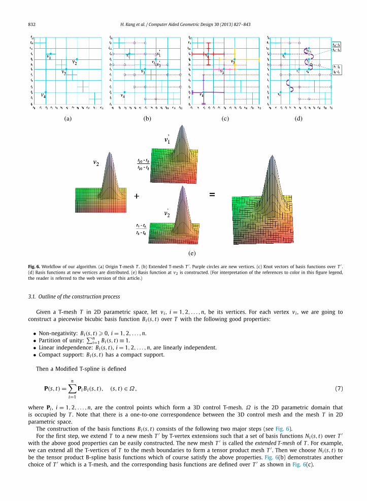
Fig. 6. Workflow of our algorithm. (a) Origin T-mesh T . (b) Extended T-mesh T ′ . Purple circles are new vertices. (c) Knot vectors of basis functions over T ′ .(d) Basis functions at new vertices are distributed. (e) Basis function at v2 is constructed. (For interpretation of the references to color in this figure legend,the reader is referred to the web version of this article.)

3.1. Outline of the construction process

Given a T-mesh T in 2D parametric space, let vi , i = 1,2, . . . ,n, be its vertices. For each vertex vi , we are going toconstruct a piecewise bicubic basis function Bi(s, t) over T with the following good properties:

• Non-negativity: Bi(s, t)� 0, i = 1,2, . . . ,n.• Partition of unity:

∑ni=1 Bi(s, t) ≡ 1.

• Linear independence: Bi(s, t), i = 1,2, . . . ,n, are linearly independent.• Compact support: Bi(s, t) has a compact support.

Then a Modified T-spline is defined

P(s, t) =n∑

i=1

Pi Bi(s, t), (s, t) ∈ Ω, (7)

where Pi , i = 1,2, . . . ,n, are the control points which form a 3D control T-mesh. Ω is the 2D parametric domain thatis occupied by T . Note that there is a one-to-one correspondence between the 3D control mesh and the mesh T in 2Dparametric space.

The construction of the basis functions Bi(s, t) consists of the following two major steps (see Fig. 6).For the first step, we extend T to a new mesh T ′ by T-vertex extensions such that a set of basis functions Ni(s, t) over T ′

with the above good properties can be easily constructed. The new mesh T ′ is called the extended T-mesh of T . For example,we can extend all the T-vertices of T to the mesh boundaries to form a tensor product mesh T ′ . Then we choose Ni(s, t) tobe the tensor product B-spline basis functions which of course satisfy the above properties. Fig. 6(b) demonstrates anotherchoice of T ′ which is a T-mesh, and the corresponding basis functions are defined over T ′ as shown in Fig. 6(c).

H. Kang et al. / Computer Aided Geometric Design 30 (2013) 827–843 833

Fig. 7. Basis function at v ′1 is distributed to basis functions at its two receiving vertices v2 and v5.

For the second step, let {v ′i}l

i=1 be the new vertices generated by the T-vertex extensions. We distribute the basis functionNi(s, t) at v ′

i to the basis functions at the neighboring old vertices of T ′ . In Fig. 6(d), the basis function at v ′1 is distributed

to the basis functions at v2 and v5, and the basis function at v ′2 is distributed to the basis functions at v2 and v6. Finally,

the basis function Bi(s, t) over T is constructed as a linear combination of the basis functions Ni(s, t) at the neighboringvertices of vi . Fig. 6(e) illustrates the basis function at v2.

The distribution of a basis function at a new vertex is composed of two steps: finding receiving vertices in T andcomputing distribution coefficients. Each new vertex is one of the three types: H-type, V-type and C-type. For H-type andV-type new vertices, the rule of distribution is simple: we distribute the basis function along one direction and performthe distribution as knot deletion in one dimension. However, for C-type new vertices, the situation is much harder. In ourconstruction, we will avoid such situation.

For example, as illustrated in Fig. 6(d), v ′1 is a H-type vertex, the basis function at v ′

1 is distributed along t (vertical)direction, and the distribution coefficients are computed by knot deletion in t direction as shown in formula (3). That isv2 and v5 are the receiving vertices of v ′

1. The distribution coefficient of v ′1 to v2 is the ratio of distance v ′

1 v5 over v2 v5

(= t10−t9t10−t8

), and the one of v ′1 to v5 is the ratio of distance v ′

1 v2 over v5 v2 (= t9−t8t10−t8

). Fig. 7 illustrates the distributionprocess of v ′

1 by formula (3).

3.2. Construction method

In this section, we present details to construct bicubic Modified T-splines.Given an original T-mesh T , we extend all the horizontal (or vertical) T-vertices to the boundary of T to obtain a

new T-mesh. Now the new T-mesh has only vertical (or horizontal) T-vertices. For such T-meshes, we have the followingimportant observation.

Lemma 3.1. If there are only vertical (horizontal) T-vertices in a mesh T , then the blending functions of the T-splines defined over Tare linearly independent and form a partition of unity.

Proof. Without loss of generality, we assume T has only vertical T-vertices. Let T ′ be the tensor product mesh by extendingall the T-vertices in T to the boundary of T . Because there are only vertical T-vertices in T , all the new vertices in T ′ areV-type. Let Bi(s, t) = N3

i (s)N3i (t) be the tensor product B-spline basis function at each vertex vi of T ′ , i = 1,2, . . . ,m. Let

Ti(s, t) be the T-spline blending function at the vertex of T , i = 1,2, . . . ,n. We are going to show that: (1) Ti(s, t) is a linearcombination of Bi(s, t), that is, there exists a matrix Mn×m such that⎛

⎝ T1...

Tn

⎞⎠ = M

⎛⎝ B1

...

Bm

⎞⎠ . (8)

(2) the matrix M has full rank and the column sums of the matrix M are all one. Then by Lemma 2.1, the assertion of thelemma follows.

Assume there are p horizontal grid lines and q vertical grid lines in T ′ . For each horizontal grid line t = ti , there are qvertices on the grid line, among which we assume ri vertices (ri � q) are old vertices. Since the T-splines at all the verticeson the grid line have the same local knot vector ti = [ti−2, ti−1, ti, ti+1, ti+2] in t direction, by the knot insertion algorithm ofunivariate cubic B-splines, the T-spline blending function Tij(s, t) at each old vertex on the grid line is a linear combinationof the blending functions Bij(s, t) at all the vertices on the grid line, that is,⎛

⎝ Ti1...

Tiri

⎞⎠ = Mi

⎛⎝ Bi1

...

Biq

⎞⎠

where the matrix Mi has full rank and the column sums of Mi are all one by the property of knot insertion. Now (8) followswith M = diag(M1, M2, . . . , Mp). Obviously, M has full rank and the column sums of M are all one. �

834 H. Kang et al. / Computer Aided Geometric Design 30 (2013) 827–843

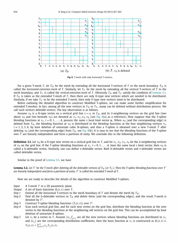
Fig. 8. T-mesh with only horizontal T-vertices.

For a given T-mesh T , let T H be the mesh by extending all the horizontal T-vertices of T to the mesh boundary. T H iscalled the horizontal extension mesh of T . Similarly, let T V be the mesh by extending all the vertical T-vertices of T to themesh boundary, and T V is called the vertical extension mesh of T . Obviously T H and T V satisfy the condition of Lemma 3.1.If T H is taken as the extended T-mesh of T , then there are only H-type new vertices which are needed to be distributed.Similarly, if we take T V to be the extended T-mesh, then only V-type new vertices need to be distributed.

Before outlining the detailed algorithm to construct Modified T-splines, we can make some further simplification forextended T-meshes. In fact, among all the new vertices in T H or T V , many can be deleted without distribution process. Wecall such vertices deletable vertices. The key observation is as follows.

Assume v0 is a H-type vertex on a vertical grid line s = si in T H , and its 2-neighboring vertices on the grid line (twoabove v0 and two beneath v0) are denoted as v1, v2, v3, v4 (see Fig. 8(a) as a reference). Now suppose that the T-splineblending functions at vi , i = 0,1, . . . ,4, possess the same s local knot vector si . When v0 (and the corresponding edge) isdeleted from T H , the blending function at v0 is distributed to the blending functions at the four neighboring vertices vi ,i = 1,2,3,4, by knot deletion of univariate cubic B-splines, and thus a T-spline is obtained over a new T-mesh T afterdeleting v0 (and the corresponding edge) from T H , see Fig. 8(b). It is easy to see that the blending functions of the T-splineover T are linearly independent and form a partition of unity. We conclude this in the following definition.

Definition 3.1. Let v0 be a H-type new vertex on a vertical grid line in T , and let v1, v2, v3, v4 be the 2-neighboring verticesof v0 on the grid line. If the T-spline blending functions at vi , i = 0,1, . . . ,4, have the same local s knot vector, then v0 iscalled a h-deletable vertex. Similarly, one can define v-deletable vertex. Both h-deletable vertex and v-deletable vertex arecalled deletable vertex.

Similar to the proof of Lemma 3.1, we have

Lemma 3.2. Let T ′ be the T-mesh after deleting all the deletable vertices of T H (or T V ). Then the T-spline blending functions over T ′are linearly independent and form a partition of unity. T ′ is called the extended T-mesh of T .

Now we are ready to describe the details of the algorithm to construct Modified T-splines.

Input A T-mesh T in a 2D parametric plane.Output A set of basis functions Bi(s, t) over T .Step 1 Extend all the horizontal T-vertices to the mesh boundary of T and denote the mesh by T H .Step 2 Find all the h-deletable vertices in T H and delete them (and the corresponding edges), and the result T-mesh is

denoted by T ′ .Step 3 Construct T-spline blending functions {Ti(s, t)} over T ′ .Step 4 Scan each vertical grid line, and for each new vertex on the grid line, distribute the blending function at the new

vertex to the blending functions at the neighboring old vertices on the grid line. This can be accomplished by knotdeletion of univariate B-splines.

Step 5 Let vi be a vertex in T . Assume {vi j }lj=1 are all the new vertices whose blending functions are distributed to vi ,

and {ci j } are the corresponding distribution coefficients, then the basis function at vi is constructed as Bi(s, t) =Ti(s, t) + ∑l

j=1 ci Ti (s, t).

j j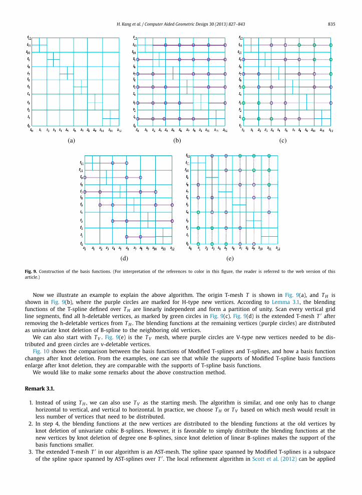

H. Kang et al. / Computer Aided Geometric Design 30 (2013) 827–843 835

Fig. 9. Construction of the basis functions. (For interpretation of the references to color in this figure, the reader is referred to the web version of thisarticle.)

Now we illustrate an example to explain the above algorithm. The origin T-mesh T is shown in Fig. 9(a), and T H isshown in Fig. 9(b), where the purple circles are marked for H-type new vertices. According to Lemma 3.1, the blendingfunctions of the T-spline defined over T H are linearly independent and form a partition of unity. Scan every vertical gridline segments, find all h-deletable vertices, as marked by green circles in Fig. 9(c). Fig. 9(d) is the extended T-mesh T ′ afterremoving the h-deletable vertices from T H . The blending functions at the remaining vertices (purple circles) are distributedas univariate knot deletion of B-spline to the neighboring old vertices.

We can also start with T V . Fig. 9(e) is the T V mesh, where purple circles are V-type new vertices needed to be dis-tributed and green circles are v-deletable vertices.

Fig. 10 shows the comparison between the basis functions of Modified T-splines and T-splines, and how a basis functionchanges after knot deletion. From the examples, one can see that while the supports of Modified T-spline basis functionsenlarge after knot deletion, they are comparable with the supports of T-spline basis functions.

We would like to make some remarks about the above construction method.

Remark 3.1.

1. Instead of using T H , we can also use T V as the starting mesh. The algorithm is similar, and one only has to changehorizontal to vertical, and vertical to horizontal. In practice, we choose T H or T V based on which mesh would result inless number of vertices that need to be distributed.

2. In step 4, the blending functions at the new vertices are distributed to the blending functions at the old vertices byknot deletion of univariate cubic B-splines. However, it is favorable to simply distribute the blending functions at thenew vertices by knot deletion of degree one B-splines, since knot deletion of linear B-splines makes the support of thebasis functions smaller.

3. The extended T-mesh T ′ in our algorithm is an AST-mesh. The spline space spanned by Modified T-splines is a subspaceof the spline space spanned by AST-splines over T ′ . The local refinement algorithm in Scott et al. (2012) can be applied

836 H. Kang et al. / Computer Aided Geometric Design 30 (2013) 827–843

Fig. 10. (a) Left to right: the extended T-mesh T ′ , the original T-mesh T and the original T-mesh T . For (b), (c) and (d), left to right: basis functions ofT-splines over T ′ , Modified T-splines and T-splines over T at three vertices v1, v2 and v3.

to obtain an AST-mesh from a given T-mesh, so AST-mesh can be used as a starting point instead of T H or T V . But asstated previously, it may introduce C-type new vertices which is hard to handle.

4. The construction algorithm involves three T-meshes: the origin T-mesh T and two auxiliary T-meshes: T H and theextended T-mesh T ′ . T H is served for constructing T ′ and T ′ is served for defining the T-splines, from which ModifiedT-splines are defined on T . At every vertex in T , a Modified T-spline basis function is defined as a linear combinationof T-spline basis functions on T ′ , and thus the knot vectors and the distribution coefficients at the new vertices in T ′are enough for further use. So it is not necessary to store the whole information of T ′ along with the original T-mesh.Both T H and T ′ are discarded after the algorithm.

3.3. Algorithm analysis

While it is generally very hard to give a complete analysis of the algorithm complexity for constructing Modified T-splines, we present several typical examples of meshes to get a hint about the algorithm complexity.

The construction algorithm in Section 3.2 mainly includes two parts: extended T-mesh T ′ construction and non-deletablevertices distribution. Let R = N

M , where N is the total number of new vertices in T ′ , and M is the total number of old verticesin T ′ (i.e., M is the total number of vertices in T ). The ratio R gives a rough idea about the computational complexity ofthe algorithm.

Fig. 11 shows four typical hierarchical T-meshes. Denote the maximum level of hierarchy by k and the refinement domainat level i by Ωi . The refinement domain Ωi in Fig. 11(a) is a rectangle with Ωi ⊂ Ωi−1 (assume that the boundaries of Ωi

and Ωi−1 do not overlap). There are 4k non-deletable vertices in T H and at least 25 + 16k old vertices in T H . So the ratioR � 4k

25+16k < 1/4. The T-mesh in Fig. 11(b) is similar to the one in Fig. 11(a), where the refinement domains are polygons.

In this case, there are 7k − 1 non-deletable vertices in T H and 30k + 36 old vertices in T H . So the ratio R = 7k−130k+36 < 7

30 .

For the mesh in Fig. 11(c), suppose that there are 2(n + 2) vertical T-vertices at level 1. Then there are nl = 2ln + 4vertical T-vertices and

∑0.5nlj=1 6 j + 3 old vertices at level l, l = 1,2, . . . ,k. We assume that k � 3. A vertical T-vertex at level l

(1 � l � k − 2) produces 13 non-deletable vertices at most, and produces 11 non-deletable vertices at most at level k − 1.At level k there are about half of vertical T-vertices, each of which produces one non-deletable vertex. So the total numberof new vertices in T ′ is less than

∑k−2l=1 13(2ln + 4) + 11(2k−1n + 4) + 0.5(2kn + 4) ≈ 12.5n · 2k + 52k. Since there are about∑k

l=1 6nl + 3n2l ≈ n2 · 4k + 18n · 2k + 24k old vertices, we get an estimate for the ratio R ≈ 12.5n·2k+52k

n2·4k+18n·2k+24k. It is easy to see

that R decreases as k increases, and R tends to zero when k is large enough.The final example illustrates the worst case – a T-mesh which refines along a diagonal as shown in Fig. 11(d), where

the band width of the refinement domain Ωi is 3. Suppose the starting mesh is an n × n TP-mesh and k � 3. Then thereare 2ln − 4 vertical T-vertices and 11(2l−1n − 2) + 16 old vertices at level l, l = 1,2, . . . ,k. A vertical T-vertex at level l(1 � l � k − 2) produces 11 non-deletable vertices at most, and produces 8 non-deletable vertices at most at level k − 1.There are about half of vertical T-vertices at level k, each of which produces one non-deletable vertex. So the new vertices inT ′ is about

∑k−2 11(2ln − 4)+ 8(2k−1n − 4)+ 0.5(2kn − 4) = 20n · 2k−1 − 22n − 44k + 54. On the other hand, there are about

l=1

H. Kang et al. / Computer Aided Geometric Design 30 (2013) 827–843 837

Fig. 11. Mesh T and the extended mesh T ′ with the ratio R, R ′ . (a) R ≈ 0.02, R ′ ≈ 0.008 with k = 2. (b) R ≈ 0.17, R ′ ≈ 0.08 with k = 4. (c) R ≈ 0.2, R ′ ≈ 0.1with n = 2 and k = 3. (d) R ≈ 0.33, R ′ ≈ 0.1 with n = 4 and k = 3.

Fig. 12. Supports of Modified T-spline basis functions.

∑kl=1 11(2l−ln − 2) + 16 = 22n · 2k−1 − 11n − 6k old vertices. So we have R ≈ 20n·2k−1−44k

22n·2k−1−6k. One can see that R approaches

1011 when k is large enough.

The number of additional control points can be quite large and may lead the refined mesh be a tensor product mesh us-ing the local refinement of T-splines (Sederberg et al., 2003). So here we will give another ratio R ′ = N

TN to give an intuitionalexpression of how big the refinement region in T ′ , where N is the total number of new vertices in T ′ , and TN is the totalnumber of vertices in the corresponding tensor product mesh. For the case in Fig. 11(a), the ratio is R ′ = 4k

(5+2k)2 � 15+k . For

the case in Fig. 11(b), we have R ′ = 7k−1(6+3k)2 � 7

36+9k . For the case in Fig. 11(c), there are (2k+1n+4k+5)(2kn+2k+4) vertices

in the corresponding tensor product mesh, so the ratio R ′ � 12.5n2k+52k22k+1n2+2k(8k+13)n

� 12.5n2k+1n2+(8k+13)n

. For the case in Fig. 11(d),

there are (2kn + 1)2 vertices in the corresponding tensor product mesh, so the ratio R ′ � 20n2k−1−44k(2kn+1)2 � 20n

(2k+1n2+4n).

The above results provide upper bounds for the ratio R and R ′ . In practice, the ratio is much smaller as shown in Fig. 11.Next we briefly discuss the supports of Modified T-spline basis functions. Suppose that T is a hierarchical T-mesh and

the level differences between adjacent cells are at most one. Denote the corresponding tensor product mesh of T at levell by Tl . Let v be a vertex at level l, then the support of Modified T-spline basis function at v is contained in an m × nrectangular mesh grid G at Tl−1, where m,n � 3. Fig. 12 shows the supports of the Modified T-spline basis functions at fourvertices v1, v2, v3, v4, where v1 is in level 3, v2 and v3 are in level 2, and v4 is in level 1.

838 H. Kang et al. / Computer Aided Geometric Design 30 (2013) 827–843

Fig. 13. Modified T-spline and T-spline. (For interpretation of the references to color in this figure, the reader is referred to the web version of this article.)

3.4. Properties of modified T-splines

For a given T-mesh T , we have constructed a set of blending functions {Bi(s, t)}ni=1, where n is the number of vertices

in T . The constructed blending functions have the following nice properties.

Theorem 3.3. The blending functions {Bi(s, t)}ni=1 constructed in Section 3.2 have the following properties:

• C2 continuity: Bi(s, t) is C2 continuous over T , i = 1,2, . . . ,n.• Non-negativity: Bi(s, t)� 0, i = 1,2, . . . ,n.• Partition of unity:

∑ni=1 Bi(s, t) ≡ 1.

• Linear independence: Bi(s, t), i = 1,2, . . . ,n, are linearly independent.• Compact support: Bi(s, t) has compact support.

Proof. We only prove that {Bi(s, t)}ni=1 are linearly independent and form a partition of unity. We adopt the notations as in

Section 3.2.Assume the extended T-mesh T ′ has m (m > n) vertices. By Lemma 3.2, the T-spline blending functions {Ti(s, t)}m

i=1 overT ′ are linearly independent and form a partition of unity.

Without loss of generality, let v1, v2, . . . , vn be the vertices in T and vn+1, . . . , vm be the new vertices. By the construc-tion process of the blending functions {Bi(s, t)}n

i=1,

⎛⎜⎜⎜⎝

B1(s, t)B2(s, t)

...

Bn(s, t)

⎞⎟⎟⎟⎠ =

⎛⎜⎜⎜⎜⎝

1 0 0 0 c1,n+1 · · · c1m

0 1 0... c2,n+1 · · · c2m

0 0. . . 0 · · · · · · · · ·

0 0 0 1 cn,n+1 · · · cnm

⎞⎟⎟⎟⎟⎠

⎛⎜⎜⎜⎝

T1(s, t)T2(s, t)

...

Tm(s, t)

⎞⎟⎟⎟⎠ = M(T1, T2, . . . , Tm)T (9)

where∑n

i=1 ci j = 1, j = n + 1, . . . ,m.Obviously, the matrix M in (9) has full rank, and the column sums of M are all one. By Lemma 2.1, {Bi(s, t)}n

i=1 arelinearly independent and form a partition of unity. The lemma is thus proved. �Remark 3.2. In the following, we call the blending functions {Bi(s, t)}n

i=1 basis functions over a T-mesh.

Fig. 13 compares a Modified T-spline function and a T-spline function over a T-mesh. In both figures (a) and (b), thecontrol coefficients corresponding to the vertices marked by orange circles are taken as one while others are taken aszero. So the functions are actually the sum of the blending functions defined over the vertices labeled with orange circles.Figs. 13(a) and (b) depict the shapes of the Modified T-spline function and T-spline function respectively. It can be seen thatthe Modified T-spline looks more fair than the T-spline.

3.5. Approximation property

Let S = span{Bi(s, t)}ni=1 be the Modified T-spline space defined over T-mesh T , where Bi(s, t) are the basis functions

defined over T . For a given continuous function f (s, t), we would like to know the approximation error of f from S .In this section, we assume that T is a hierarchical T-mesh such that for any two neighboring cells in T , the level

difference is at most one. Ω is the rectangular parameter domain that is occupied by T . Ωl is the parametric domain thatconsists of all the cells in level l. hl is the maximum length of the cells in level l.

H. Kang et al. / Computer Aided Geometric Design 30 (2013) 827–843 839

Fig. 14. Conversion of Modified T-spline surfaces to TP-spline surfaces.

Theorem 3.4. For any continuous function f ∈ C(Ω), there exists a Modified T-spline function g(s, t) ∈ S such that∣∣ f (s, t) − g(s, t)∣∣ � C w( f ,hl), (s, t) ∈ Ωl. (10)

Here w( f ,h) is the modulus of continuity of f , that is, w( f ,h) = max‖x−y‖2�h | f (x) − f (y)|. C is a constant which is independentof the mesh T .

Proof. For any function f , define

A f (s, t) =n∑

i=1

f (ξi, ηi)Bi(s, t),

where (ξi, ηi) are the coordinates of the vertex in T corresponding to the basis function Bi(s, t).Let θ ⊂ Ωl be a cell in level l. For any (s, t) ∈ θ , we have

f (s, t) − A f (s, t) = f (s, t) −∑i∈K

f (ξi, ηi)Bi(s, t)

=∑i∈K

[f (s, t) − f (ξi, ηi)

]Bi(s, t)

� maxi∈K

∣∣ f (s, t) − f (ξi, ηi)∣∣

by the partition of unity of basis functions. Here K = {i | Bi(s, t) �= 0, 1 � i � n}.Now suppose θ is contained in a cell θ ′ at level l −1. Denote the corresponding tensor product mesh of T at level l −1 as

Tl−1. Then there is a 3 × 3 rectangular mesh grid G in Tl−1 whose central cell is θ ′ , and the B-spline basis functions at thevertices of G do not vanish in θ . If G doesn’t contain new vertices of T ′ (extended T-mesh of T ), then {(ξi, ηi) | i ∈ K } ⊂ G ,so

maxi∈K

∣∣ f (s, t) − f (ξi, ηi)∣∣ � w( f ,3

√2hl−1) � (3

√2 + 1)w( f ,hl−1).

For a hierarchical T-mesh, we generally have hl � hl−1/2. Therefore∣∣ f (s, t) − A f (s, t)∣∣ � (3

√2 + 1)w( f ,hl−1)� 2(3

√2 + 1)w( f ,hl). (11)

840 H. Kang et al. / Computer Aided Geometric Design 30 (2013) 827–843

Fig. 15. Fitting open mesh models with Modified T-splines.

Table 1Statistic data for fitting mesh models.

Mesh model #Points #Faces #CP #Levels

Horse 4750 9369 898 7Man 9104 18 092 1585 6Female 6301 12 487 1067 8

When G contains new vertices of T ′ , then there exist Modified T-spline basis functions outside of G whose supports con-tain θ . So we have to enlarge G . Such changes only influence the const C in (10). Fortunately, according to the distributionprocess, if the level difference between adjacent cells is at most one, G does not need to be enlarged. �4. Applications

4.1. Conversion of Modified T-splines to TP-splines

Since Modified T-spline basis functions {Bi(s, t)}ni=1 are linear combinations of the T-spline functions {Ti(s, t)}m

i=1, and byknot insertion, the T-spline functions {Ti(s, t)}m

i=1 are linear combinations of the TP B-spline basis functions {Ni(s, t)}li=1, so

{Bi(s, t)}n are linear combinations of {Ni(s, t)}l . In matrix form,

i=1 i=1

H. Kang et al. / Computer Aided Geometric Design 30 (2013) 827–843 841

Fig. 16. NURBS approximation. (a) The original NURBS surface with 504 control points. (b) and (c) A Modified T-spline approximation with 184 controlpoints and ε = 2.9%. (d) and (e) A Modified T-spline approximation with 343 control points and ε = 1.8%. (For interpretation of the references to color inthis figure, the reader is referred to the web version of this article.)

Fig. 17. NURBS approximation. (a) The original NURBS surface with 2096 control points. (b) and (c) A Modified T-spline approximation with 714 controlpoints and ε = 1.61%. (For interpretation of the references to color in this figure, the reader is referred to the web version of this article.)

(B1, . . . , Bn)T = M(T1, . . . , Tm)T ,

(T1, . . . , Tm)T = L(N1, . . . , Nl)T .

Thus

(B1, . . . , Bn)T = ML(N1, . . . , Nl)

T .

Suppose we have a Modified T-spline surface

S(s, t) =n∑

i=1

Pi Bi(s, t) = (P1, . . . ,Pn)(B1, . . . , Bn)T ,

then it can be converted into a TP B-spline surface:

S(s, t) =l∑

i=1

Qi Ni(s, t) = (Q1, . . . ,Ql)(N1, . . . , Nl)T ,

where (Q1, . . . ,Ql) = (P1, . . . ,Pm)ML.

842 H. Kang et al. / Computer Aided Geometric Design 30 (2013) 827–843

This conversion makes it easy for Modified T-splines to be conveniently imported into the current surface modelingsystem. Fig. 14 shows the conversion results of the Modified T-spline surface. Here the curves on the surfaces in column (b)are the images of the T-mesh, and the curves on the surface in column (c) are the images of tensor product mesh.

4.2. Fitting open meshes

Suppose we are given an open mesh model with vertices Pi , i = 1,2, . . . , N , in 3D space, and their corresponding param-eter values (si, ti), i = 1,2, . . . , N , obtained from some parameterization of the mesh (we use the method in Floater, 1997,in the current paper). The parameter domain is assumed to be [0,1] × [0,1].

The surface fitting scheme repeats the following steps 2 and 3 until the fitting error in each cell is less than sometolerance ε.

1. Construct a uniform tensor product mesh T0 as the initial mesh. Set k = 0.2. Solve a least square fitting problems on the kth level mesh Tk to find a Modified T-spline surface Sk(s, t) to fit the given

mesh model.3. Search for the cells of the T-mesh Tk whose fitting errors are greater than ε, then split these cells into four sub-cells to

obtain a new mesh Tk+1. The fitting error over a cell s is defined to be max(si ,ti)∈s ‖Pi − Sk(si, ti)‖. Set k := k + 1.

Fig. 15 illustrates three examples for fitting open meshes with Modified T-splines, and Table 1 shows the statistic dataincluding the number points/faces of the mesh models, the number of control points of the fitting spline surfaces and thefitting level.

4.3. NURBS approximation

The surface fitting scheme provided in the previous subsections can be easily adapted to approximate a NURBS modelwith a Modified T-spline surface. We illustrate two examples as shown in Figs. 16 and 17. In each example, the approxima-tion error ε and the number of control points in the approximating Modified T-spline are provided. Here the control nets ofNURBS surface are displayed in bright green, and the one of the Modified T-splines are in pink. From the examples, it canbe seen that there is a considerable reduction of control points of Modified T-splines compared with NURBS representations.

5. Conclusions and future work

This paper proposes a new local refinement splines called Modified T-splines. The basic idea is to construct a set of basisfunctions over a T-mesh which have good properties such as non-negativity, partition of unity and compact support. Due tothe properties of the basis functions, Modified T-splines inherit many good properties of current local refinement splines,and thus should be useful both in geometric modeling and isogeometric analysis.

There are a few problems worthy of further investigation. First, the local refinement algorithm is crucial in adaptivemodeling and analysis of splines. We will discuss the local refinement algorithm for Modified T-splines. Second, in thecurrent construction, the Modified T-splines are C2 continuous globally. We will investigate the possibility to insert multipleknots such that C0 or C1 continuity could be achieved at the knot lines, i.e., we will consider Modified T-splines overμ-extended box partitions (Dokken et al., 2013). Finally, we will investigate further applications of Modified T-splines ingeometric modeling and isogeometric analysis.

Acknowledgements

The authors thank the reviewers for providing useful comments and suggestion. The work is supported by 973 Program2011CB302400, the NSF of China No. 11031007.

References

Bazilevs, Y., Calo, V.M., Cottrell, J.A., Evans, J.A., Hughes, T.J.R., Lipton, S., Scott, M.A., Sederberg, T.W., 2010. Isogeometric analysis using T-splines. Comput.Methods Appl. Mech. Eng. 199 (5–8), 229–263.

Buffa, A., Cho, D., Sangalli, G., 2010. Linear independence of the T-spline blending functions associated with some particular T-meshes. Comput. MethodsAppl. Mech. Eng. 199, 1437–1445.

Cottrell, J.A., Hughes, T.J.R., Bazilevs, Y., 2009. Isogeometric Analysis: Toward Integration of CAD and FEA. Wiley, Chichester.Deng, Jiansong, Chen, Falai, Li, Xin, Hu, Changqi, Tong, Weihua, Yang, Zhouwang, Feng, Yuyu, 2008. Polynomial splines over hierarchical T-meshes. Graph.

Models 70, 76–86.Dokken, T., Lyche, Tom, Pettersen, Kjell Fredrik, 2013. Polynomial splines over locally refined box-partitions. Comput. Aided Geom. Des. 30, 331–356.Dörfel, M., Jüttler, B., Simeon, B., 2009. Adaptive isogeometric analysis by local h-refinement with T-splines. Comput. Methods Appl. Mech. Eng. 199 (5–8),

264–275.Floater, Michael S., 1997. Parametrization and smooth approximation of surface triangulations. Comput. Aided Geom. Des. 14, 231–250.Forsey, D.R., Bartels, R.H., 1988. Hierarchical B-spline refinement. Comput. Graph. 22 (4), 205–212.Giannelli, Carlotta, Jüttler, Bert, Speleers, Hendrik, 2012. THB-splines: The truncated basis for hierarchical splines. Comput. Aided Geom. Des. 29 (7),

485–498.

H. Kang et al. / Computer Aided Geometric Design 30 (2013) 827–843 843

Hughes, T.J.R., Cottrell, J.A., Bazilevs, Y., 2005. Isogeometric analysis: CAD, finite elements, NURBS, exact geometry, and mesh refinement. Comput. MethodsAppl. Mech. Eng. 194, 4135–4195.

Li, Xin, Zheng, Jianming, Sederberg, T.W., Hughes, T.J.R., Scott, M.A., 2012. On the linear independence of T-spline blending functions. Comput. Aided Geom.Des. 29 (1), 63–76.

Nguyen-Thanh, N., Nguyen-Xuan, H., Bordasd, S.P.A., Rabczuk, T., 2011a. Isogeometric analysis using polynomial splines over hierarchical T-meshes fortwo-dimensional elastic solids. Comput. Methods Appl. Mech. Eng. 200 (21–22), 1892–1908.

Nguyen-Thanh, N., Kiendl, J., Nguyen-Xuan, H., Wüchner, R., Bletzinger, K.U., Bazilevs, Y., Rabczuk, T., 2011b. Rotation free isogeometric thin shell analysisusing PHT-splines. Comput. Methods Appl. Mech. Eng. 200 (47–48), 3410–3424.

Scott, M.A., Li, X., Sederberg, T.W., Hughes, T.J.R., 2012. Local refinement of analysis-suitable T-splines. Comput. Methods Appl. Mech. Eng. 213–216, 206–222.Sederberg, T., Zheng, J., Bakenov, A., Nasri, A., 2003. T-splines and T-NURCCSs. ACM Trans. Graph. 22 (3), 477–484.Sederberg, T., Cardon, D., Finnigan, G., North, N., Zheng, J., Lyche, T., 2004. T-spline simplification and local refinement. ACM Trans. Graph. 23 (3), 276–283.