computer vision object and people...
TRANSCRIPT

Feature Descriptors
Prof. Didier Stricker
Dr. Alain Pagani
Kaiserlautern University
http://ags.cs.uni-kl.de/
DFKI – Deutsches Forschungszentrum für Künstliche Intelligenz
http://av.dfki.de
Computer Vision
Object and People Tracking
1

Previous lectures: Feature extraction
Gradient/edge
Points (Kanade-Tomasi + Harris)
Blob (incl. scale)
Today: Feature Descriptors
Why? Point matching
Region and image matching
Overview
2

Problem: For each point correctly recognize the
corresponding one
Matching with Features
?
We need a reliable and distinctive descriptor!
3

We know how to detect good points
Next question: How to match them?
Answer: Come up with a descriptor for each point, find
similar descriptors between the two images
Feature descriptors
?
4

We know how to detect good points
Next question: How to match them?
Lots of possibilities (this is a popular research area) Simple option: match square windows around the point
State of the art approach: SIFT David Lowe, UBC http://www.cs.ubc.ca/~lowe/keypoints/
Feature descriptors
?
5

Invariance: Descriptor shouldn’t change even if image is
transformed
Discriminability: Descriptor should be highly unique for each
point
Invariance vs. discriminability
6
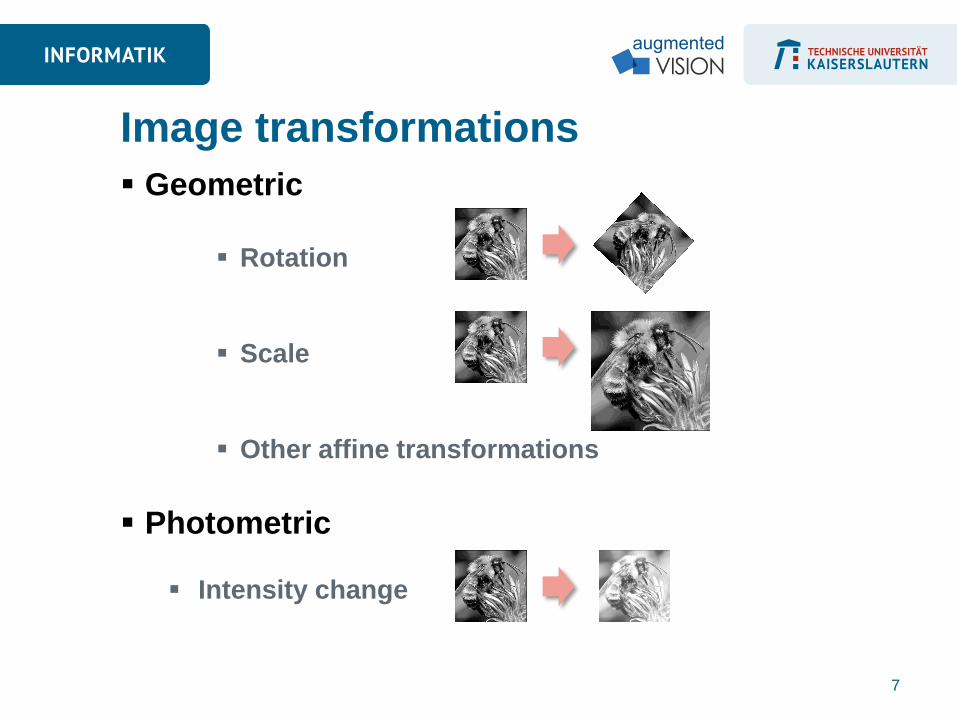
Geometric
Rotation
Scale
Other affine transformations
Photometric
Intensity change
Image transformations
7

Most feature descriptors are designed to be
invariant to Translation
2D rotation
Scale
They can usually also handle Limited 3D rotations (SIFT works up to
about 60 degrees)
Limited affine transformations (some are
fully affine invariant)
Limited illumination/contrast changes
Invariance
8

Need both of the following:
1. Make sure your detector is invariant
2. Design an invariant feature descriptor
Simplest descriptor: a single pixel value What’s this invariant to?
Is this unique?
Next simplest descriptor: a square
window of pixels Is this unique?
What’s this invariant to?
Let’s look at some better approaches…
How to achieve invariance
9

L1 – Sum of Absolute Differences (SAD)
L2 – Sum of Squared Differences (SSD)
Cross-Correlation
Comparing two patches
10

Sum of Absolute Differences (SAD) – L1 norm
Sum of Squared Differences (SSD) – L2 norm
Common window-based approaches
𝐼1 𝑖, 𝑗 − 𝐼2(𝑥 + 𝑖, 𝑦 + 𝑗)
(𝑖,𝑗)∈𝑊
𝐼1 𝑖, 𝑗 − 𝐼2(𝑥 + 𝑖, 𝑦 + 𝑗)2
(𝑖,𝑗)∈𝑊
11
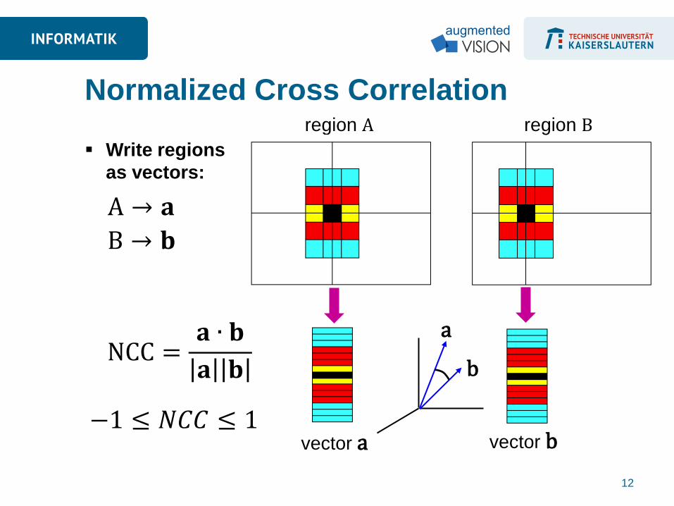
Normalized Cross Correlation region A region B
vector a vector b
a
b
12
NCC =𝐚 ∙ 𝐛
𝐚 𝐛
A → 𝐚
B → 𝐛
−1 ≤ 𝑁𝐶𝐶 ≤ 1
Write regions
as vectors:
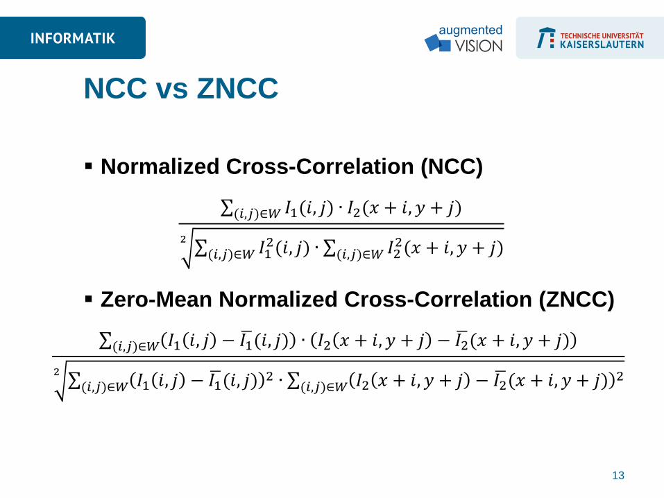
Normalized Cross-Correlation (NCC)
Zero-Mean Normalized Cross-Correlation (ZNCC)
NCC vs ZNCC
𝐼1(𝑖, 𝑗)(𝑖,𝑗)∈𝑊 ∙ 𝐼2(𝑥 + 𝑖, 𝑦 + 𝑗)
𝐼12(𝑖, 𝑗)(𝑖,𝑗)∈𝑊 ∙ 𝐼2
2(𝑥 + 𝑖, 𝑦 + 𝑗)(𝑖,𝑗)∈𝑊2
𝐼1 𝑖, 𝑗 − 𝐼1 (𝑖, 𝑗) ∙ 𝐼2 𝑥 + 𝑖, 𝑦 + 𝑗 − 𝐼2 (𝑥 + 𝑖, 𝑦 + 𝑗)(𝑖,𝑗)∈𝑊
𝐼1 𝑖, 𝑗 − 𝐼1 (𝑖, 𝑗)2 ∙ 𝐼2 𝑥 + 𝑖, 𝑦 + 𝑗 − 𝐼2 (𝑥 + 𝑖, 𝑦 + 𝑗)
2(𝑖,𝑗)∈𝑊(𝑖,𝑗)∈𝑊
2
13
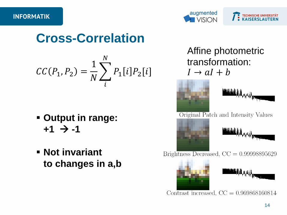
Output in range:
+1 -1
Not invariant
to changes in a,b
Cross-Correlation Affine photometric transformation:
14
𝐶𝐶 𝑃1, 𝑃2 =1
𝑁 𝑃1 𝑖 𝑃2[𝑖]
𝑁
𝑖
𝐼 → 𝑎𝐼 + 𝑏

Make each patch zero mean:
Then make unit variance:
(Zero Mean) Normalized Cross-
Correlation
15
𝐼 → 𝑎𝐼 + 𝑏
Affine photometric transformation:
𝜇 =1
𝑁 𝐼(𝑥, 𝑦)
𝑥,𝑦
𝑍 𝑥, 𝑦 = 𝐼 𝑥, 𝑦 − 𝜇
𝜎2 =1
𝑁 𝑍(𝑥, 𝑦)2
𝑥,𝑦
𝑍𝑁 𝑥, 𝑦 =𝑍(𝑥, 𝑦)
𝜎

Example with NCC
epipolar line
16

Example with NCC
left image band
right image band
cross correlation
1
0
0.5
x 17

Example with NCC
Why is it not as good
as before?
18
left image band
right image band
cross correlation
1
0
x
0.5
target region

SIFT – Scale Invariant Feature Transform
19
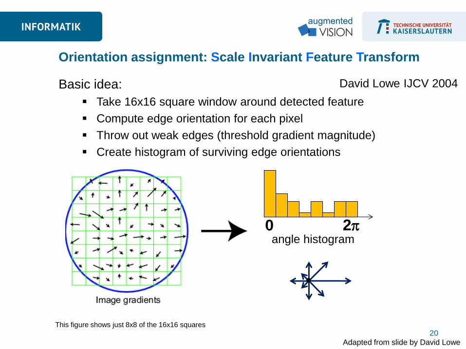
Basic idea:
Take 16x16 square window around detected feature
Compute edge orientation for each pixel
Throw out weak edges (threshold gradient magnitude)
Create histogram of surviving edge orientations
Orientation assignment: Scale Invariant Feature Transform
Adapted from slide by David Lowe
0 2 angle histogram
David Lowe IJCV 2004
This figure shows just 8x8 of the 16x16 squares
20

Create histogram of gradient directions, within a region
around the keypoint, at selected scale:
Orientation assignment
36 bins (i.e., 10º per bin)
Histogram entries are weighted by (i) gradient magnitude and (ii) a
Gaussian function with σ equal to 1.5 times the scale of the keypoint.
0 2
21
𝐿 𝑥, 𝑦, 𝜎 = 𝐺 𝑥, 𝑦, 𝜎 ∗ 𝐼(𝑥, 𝑦)
𝑚 𝑥, 𝑦 = 𝐿 𝑥 + 1, 𝑦 − 𝐿(𝑥 − 1, 𝑦) 2 + 𝐿 𝑥, 𝑦 + 1 − 𝐿(𝑥, 𝑦 − 1) 2
𝜃 𝑥, 𝑦 = atan2 𝐿 𝑥, 𝑦 + 1 − 𝐿 𝑥, 𝑦 − 1 , 𝐿 𝑥 + 1, 𝑦 − 𝐿(𝑥 − 1, 𝑦)

Orientation assignment
22

Orientation assignment
23
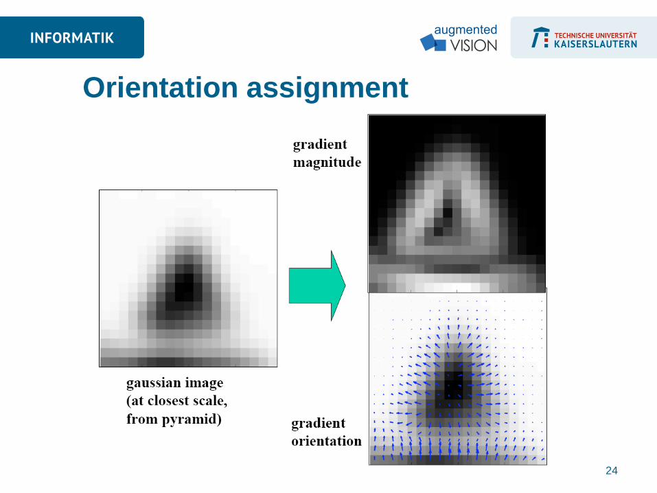
Orientation assignment
24

Orientation assignment
σ=1.5*scale of
the keypoint
25

Orientation assignment
26
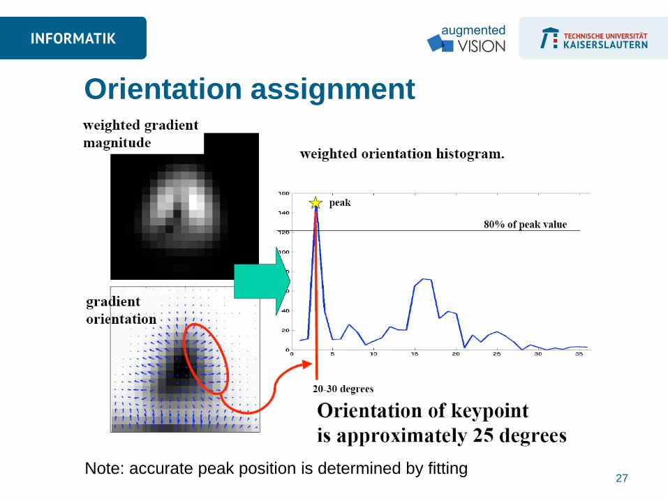
Orientation assignment
Note: accurate peak position is determined by fitting 27
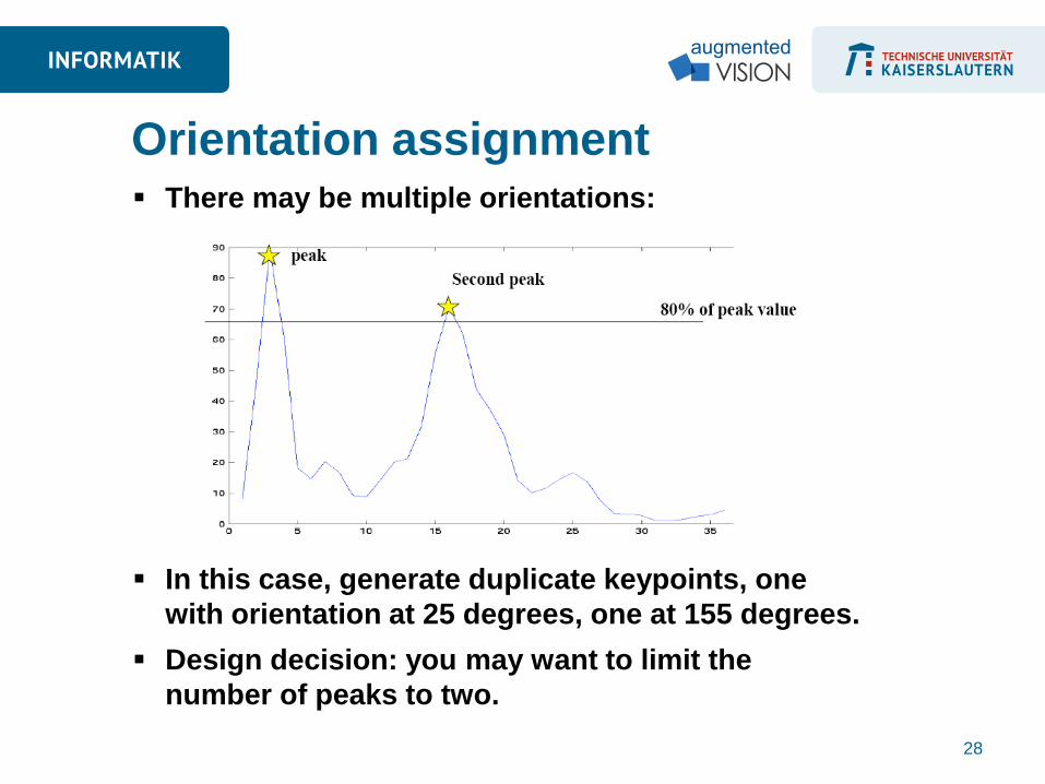
Orientation assignment There may be multiple orientations:
In this case, generate duplicate keypoints, one
with orientation at 25 degrees, one at 155 degrees.
Design decision: you may want to limit the
number of peaks to two.
28

Keypoint Descriptor
8 bins
29

Keypoint Descriptor (cont’d)
16 histograms x 8 orientations
= 128 features
1. Take a 16x16
window around
detected
interest point.
2. Divide into a
4x4 grid of
cells.
3. Compute
histogram in
each cell.
(8 bins)
30
0 2 angle histogram

Each histogram entry is weighted by
(i) gradient magnitude and
(ii) a Gaussian function with σ equal to 0.5
times the width of the descriptor window.
Keypoint Descriptor (cont’d)
31
0 2 angle histogram

Partial Voting: distribute histogram entries into
adjacent bins (i.e., additional robustness to
shifts)
Each entry is added to all bins, multiplied by a
weight of 1-d, where d is the distance from the bin
it belongs to.
Keypoint Descriptor (cont’d)
32

Keypoint Descriptor (cont’d)
128 features
Descriptor depends on two main parameters: (1) number of orientations r
(2) n x n array of orientation histograms
SIFT: r=8, n=4
rn2 features
33

Invariance to linear illumination changes: Normalization to unit length is sufficient.
Keypoint Descriptor (cont’d)
128 features
34

Non-linear illumination changes: Saturation affects gradient magnitudes more
than orientations
Threshold entries to be no larger than 0.2 and
renormalize to unit length
Keypoint Descriptor (cont’d)
128 features
35

Robustness to viewpoint changes
Additional
robustness can
be achieved using
affine invariant
region detectors.
Match features after random change in
image scale and orientation, with 2%
image noise, and affine distortion.
Find nearest neighbor in database of
30,000 features.
36

Vary size of database of features, with 30
degree affine change, 2% image noise.
Measure % correct for single nearest
neighbor match.
Distinctiveness
37
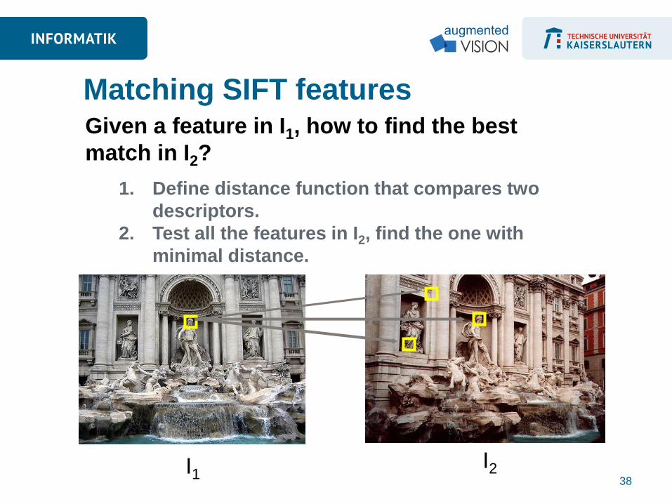
Given a feature in I1, how to find the best
match in I2?
1. Define distance function that compares two
descriptors.
2. Test all the features in I2, find the one with
minimal distance.
I1 I2
Matching SIFT features
38
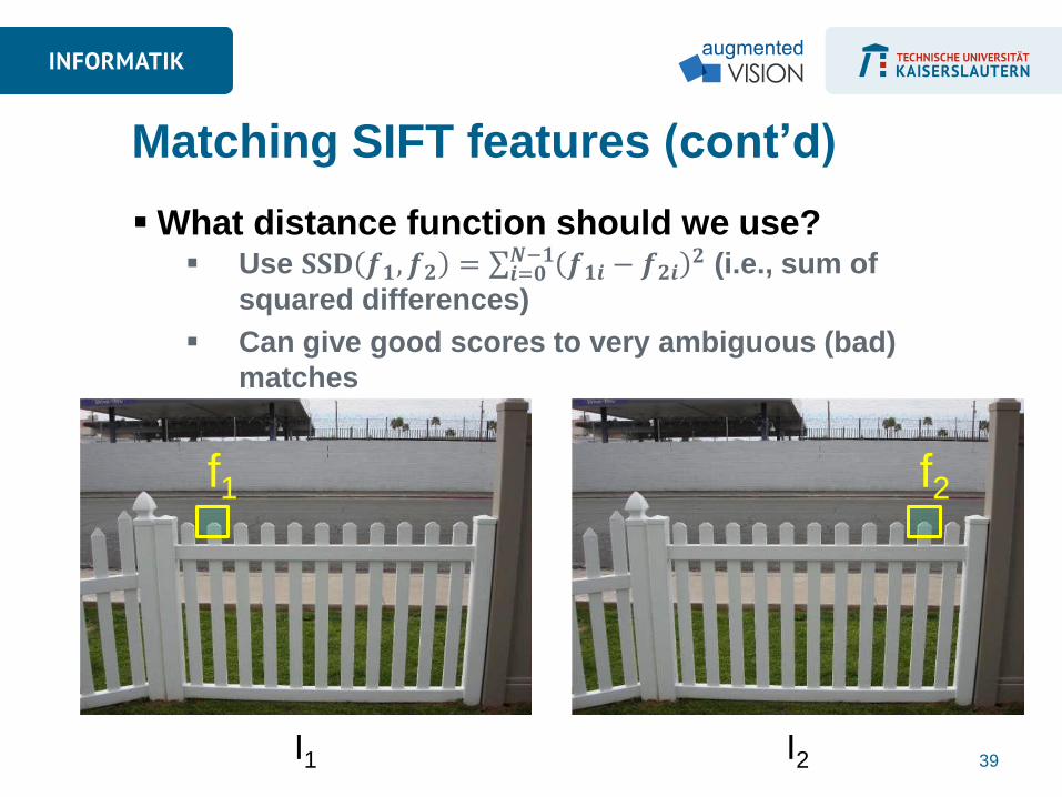
Matching SIFT features (cont’d)
I1 I2
f1 f2
What distance function should we use? Use 𝐒𝐒𝐃 𝒇𝟏, 𝒇𝟐 = 𝒇𝟏𝒊 − 𝒇𝟐𝒊
𝟐𝑵−𝟏𝒊=𝟎 (i.e., sum of
squared differences)
Can give good scores to very ambiguous (bad)
matches
39

A better distance measure is the following: 𝐒𝐒𝐃(𝒇𝟏, 𝒇𝟐) 𝐒𝐒𝐃(𝒇𝟏, 𝒇𝟐
′ )
𝒇𝟐 is best SSD match to 𝒇𝟏 in I2
𝒇𝟐′ is 2nd best SSD match to 𝒇𝟏 in I2
Matching SIFT features (cont’d)
I1 I2
f1 f2
40

Accept a match if 𝐒𝐒𝐃(𝒇𝟏, 𝒇𝟐) 𝐒𝐒𝐃(𝒇𝟏, 𝒇𝟐′ ) < 𝒕
𝒕 = 0.8 has given good results in object recognition
90% of false matches were eliminated
Less than 5% of correct matches were discarded
Matching SIFT features (cont’d)
41

(1) Scale-space extrema detection Extract scale and rotation invariant interest points (i.e.,
keypoints).
(2) Keypoint localization Determine location and scale for each interest point.
Eliminate “weak” keypoints
(3) Orientation assignment Assign one or more orientations to each keypoint.
(4) Keypoint descriptor Use local image gradients at the selected scale.
SIFT Steps – Review
D. Lowe, “Distinctive Image Features from Scale-Invariant Keypoints”,
International Journal of Computer Vision, 60(2):91-110, 2004.
Cited > 10.000 times
42
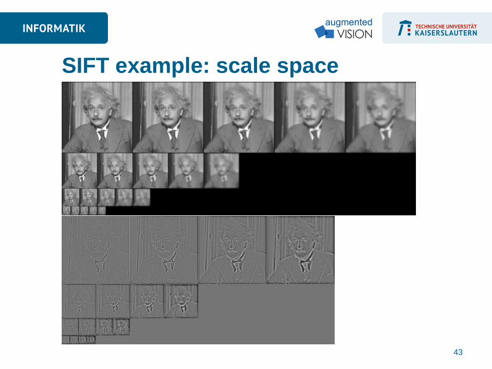
SIFT example: scale space
43

Maxima in D
44

Remove low contrast
45

Remove edges
46
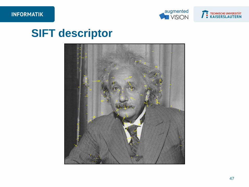
SIFT descriptor
47

48

Empirically found2 to show very good
performance, invariant to image rotation,
scale, intensity change, and robust to
moderate affine transformations
SIFT – Scale Invariant Feature Transform1
1 D.Lowe. “Distinctive Image Features from Scale-Invariant Keypoints”. Accepted to IJCV 2004 2 K.Mikolajczyk, C.Schmid. “A Performance Evaluation of Local Descriptors”. CVPR 2003
Scale = 2.5
Rotation = 45°
49
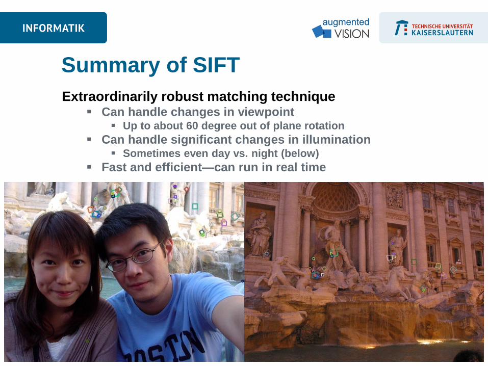
Extraordinarily robust matching technique Can handle changes in viewpoint
Up to about 60 degree out of plane rotation
Can handle significant changes in illumination Sometimes even day vs. night (below)
Fast and efficient—can run in real time
Summary of SIFT
HOG – Histogram of Oriented Gradients
51

Slide from Sminchisescu 52
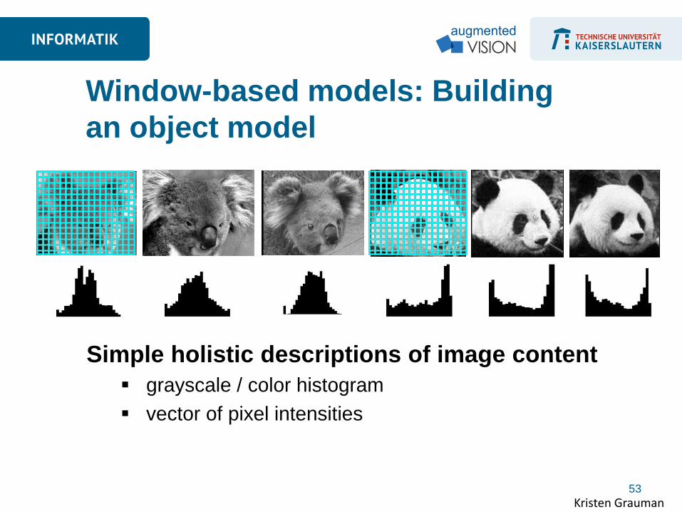
Simple holistic descriptions of image content
grayscale / color histogram
vector of pixel intensities
Kristen Grauman
Window-based models: Building
an object model
53
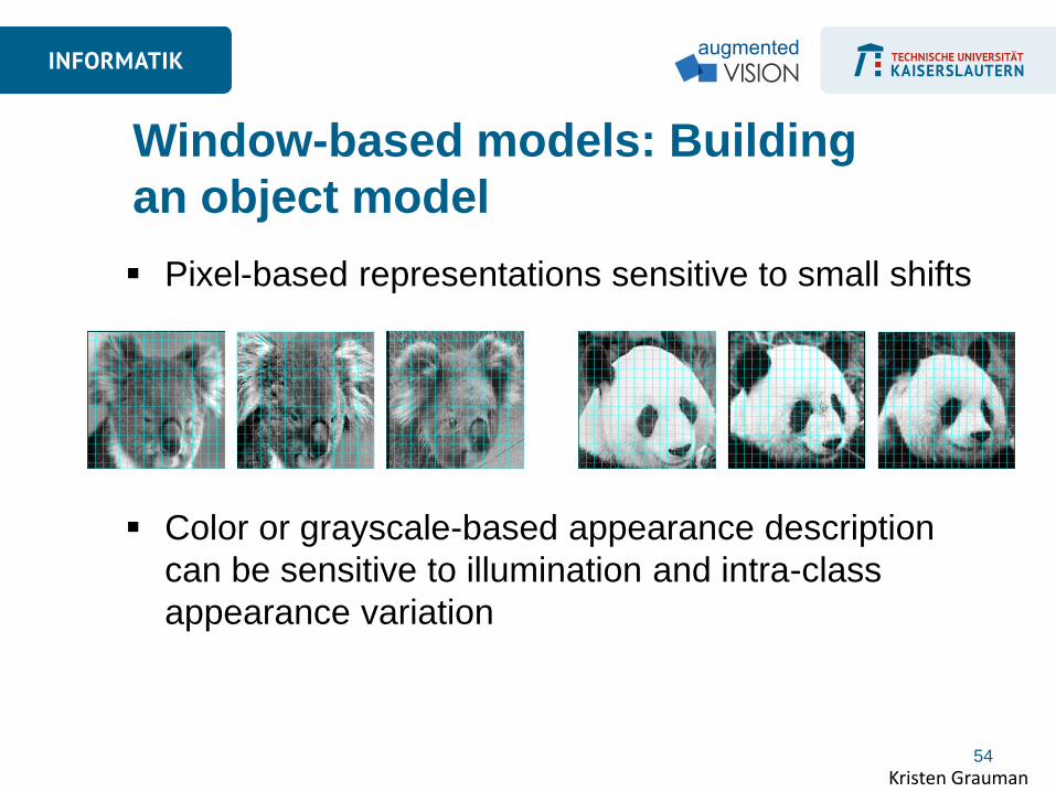
Pixel-based representations sensitive to small shifts
Color or grayscale-based appearance description
can be sensitive to illumination and intra-class
appearance variation
Kristen Grauman
Window-based models: Building
an object model
54

Consider edges, contours, and (oriented) intensity
gradients
Kristen Grauman
Window-based models: Building
an object model
55
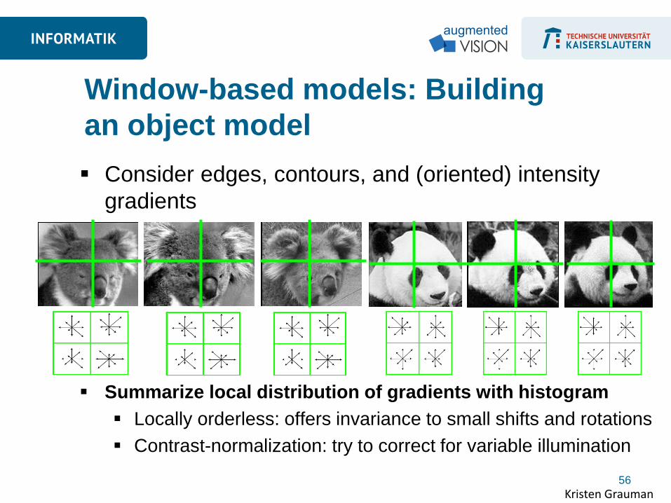
Consider edges, contours, and (oriented) intensity
gradients
Summarize local distribution of gradients with histogram
Locally orderless: offers invariance to small shifts and rotations
Contrast-normalization: try to correct for variable illumination
Kristen Grauman
Window-based models: Building
an object model
56

Gradient histograms measure the orientations and
strengths of image gradients within an image region
Global descriptor for the complete body
Very high-dimensional Typically ~4000 dimensions
Histograms
57
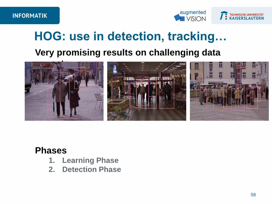
Very promising results on challenging data
sets
Phases 1. Learning Phase
2. Detection Phase
HOG: use in detection, tracking…
58

1. Compute gradients on an
image region of 64x128 pixels
2. Compute histograms on ‘cells’
of typically 8x8 pixels (i.e. 8x16
cells)
3. Normalize histograms within
overlapping blocks of cells
(typically 2x2 cells, i.e. 7x15
blocks)
4. Concatenate histograms
Descriptor
59

Convolution with [-1 0 1] filters
No smoothing
Compute gradient magnitude + direction
Per pixel: color channel with greatest magnitude
final gradient
Gradients
60

Cell histograms
9 bins for gradient orientations
(0-180 degrees)
Filled with magnitudes
Interpolated trilinearly: Bilinearly into spatial cells
Linearly into orientation bins
61
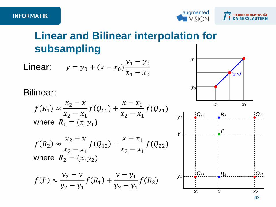
Linear and Bilinear interpolation for
subsampling
Linear:
Bilinear:
62
𝑦 = 𝑦0 + (𝑥 − 𝑥0)𝑦1 − 𝑦0𝑥1 − 𝑥0
𝑓 𝑅1 ≈𝑥2 − 𝑥
𝑥2 − 𝑥1𝑓 𝑄11 +
𝑥 − 𝑥1𝑥2 − 𝑥1
𝑓(𝑄21)
𝑅1 = (𝑥, 𝑦1) where
𝑓 𝑅2 ≈𝑥2 − 𝑥
𝑥2 − 𝑥1𝑓 𝑄12 +
𝑥 − 𝑥1𝑥2 − 𝑥1
𝑓(𝑄22)
𝑅2 = (𝑥, 𝑦2) where
𝑓 𝑃 ≈𝑦2 − 𝑦
𝑦2 − 𝑦1𝑓 𝑅1 +
𝑦 − 𝑦1𝑦2 − 𝑦1
𝑓(𝑅2)

θ=85 degrees Distance to bin centers
Bin 70 15 degrees Bin 90 5 degrees
Ratios: 5/20=1/4, 15/20=3/4
Distance to cell centers Left: 2, Right: 6 Top: 2, Bottom: 6
Ratio Left-Right: 6/8, 2/8 Ratio Top-Bottom: 6/8, 2/8 Ratios:
6/8*6/8 = 36/64 = 9/16 6/8*2/8 = 12/64 = 3/16 2/8*6/8 = 12/64 = 3/16 2/8*2/8 = 4/64 = 1/16
Histogram interpolation example
63

Overlapping blocks of 2x2 cells Cell histograms are concatenated
and then normalized Note that each cell has several occurrences with
different normalization in final descriptor
Normalization Different norms possible We add a normalization
epsilon to avoid division by zero
Blocks
64

Gradient magnitudes are
weighted according to a
Gaussian spatial window
Distant gradients contribute
less to the histogram
Blocks
65
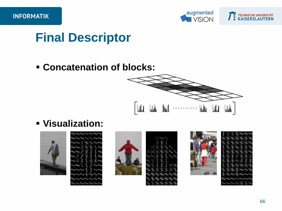
Concatenation of blocks:
Visualization:
Final Descriptor
66

Linear SVM for pedestrian detection
using the HOG descriptor
67

Slides by Pete Barnum Navneet Dalal and Bill Triggs, Histograms of Oriented Gradients for Human Detection, CVPR05 68
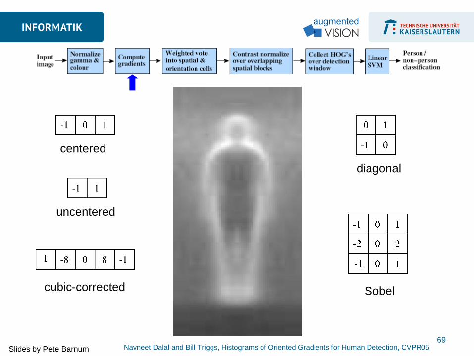
uncentered
centered
cubic-corrected
diagonal
Sobel
Slides by Pete Barnum Navneet Dalal and Bill Triggs, Histograms of Oriented Gradients for Human Detection, CVPR05 69

Histogram of gradient orientations
Orientation
Slides by Pete Barnum Navneet Dalal and Bill Triggs, Histograms of Oriented Gradients for Human Detection, CVPR05 70

15x7 cells
8 orientations
Slides by Pete Barnum Navneet Dalal and Bill Triggs, Histograms of Oriented Gradients for Human Detection, CVPR05 71
∈ ℝ840 𝑥 =

person
Slides by Pete Barnum Navneet Dalal and Bill Triggs, Histograms of Oriented Gradients for Human Detection, CVPR05 72
0.16 = 𝑤𝑇𝑥 − 𝑏
sign 0.16 = 1

Developing a feature descriptor requires a lot of
engineering Testing of parameters (e.g. size of cells, blocks, number of
cells in a block, size of overlap)
Normalization schemes (e.g. L1, L2-Norms etc., gamma
correction, pixel intensity normalization)
An extensive evaluation of different choices was
performed, when the descriptor was proposed
It’s not only the idea, but also the engineering
effort
Engineering
73

Thank you!
74