computer programming - curly-brace.com · computer programming an introduction for the...

Computer ProgrammingAn Introduction for the Scientifically Inclined

Sander Stoks

PDF version, registered to Sample Excerpt

Many of the designations used by manufacturers and sellers to distinguish their productsare claimed as trademarks. Where those designations appear in this book, and CurlyBrace Publishing was aware of a trademark claim, the designations have been printedwith initial capital letters or in all capitals.

The author and publisher have taken care in the preparation in this book, but make noexpressed or implied warranty of any kind and assume no responsibility for errors oromissions. No liability is assumed for incidental or consequential damages in connectionwith or arising out of the use of the information or programs contained herein.

The publisher offers discounts on this book when ordered in quantity for bulk purchasesand special sales. For more information, please contact [email protected]. Thisversion of the book is prepared for optimal reading on an electronic reading device withan 8" screen (such as the iLiad reader by iRex Technologies). There is also a paperbackedition of this book available, with ISBN 978- 90- 812788- 1- 2.

Visit Curly Brace Publishing on the web: http://www.curly-brace.com

Stoks, Sander.Computer Programming: An Introduction for the Scientifically Inclined / Sander StoksIncludes bibliographical references and index.ISBN 978- 90- 812788- 1- 2 (paperback edition)NUR code 989 Rev 1

Copyright c© 2008 by Curly Brace Publishing.

All rights reserved. No part of this publication may be reproduced, stored in a re-trieval system, or transmitted, in any form, or by any means, electronic, mechanical,photocopying, recording, or otherwise, without the prior consent of the publisher.

For information on obtaining permission for use of material from this work, pleasecontact [email protected].

ISBN 978- 90- 812788- 1- 2 (paperback edition)

http://www.curly-brace.com

Chapter 1

Computers

Where a calculator on the ENIAC is equipped with 18,000vacuum tubes and weighs 30 tons, computers in the future may

have only 1,000 vacuum tubes and perhaps weigh 1 12 tons.

Popular Mechanics, March 1949

1.1 Do You Need To Know?

Many programming teachers deliberately refrain from going into details aboutcomputer hardware. Their reasoning is that intimate knowledge of the waycomputers work actually hinders the development of a proper programmingstyle. In fact, many prefer working with pencil and paper instead of even usinga computer. A quote by Edsger W. Dijkstra, a famous Dutch computer scientist,is that “Computer Science is no more about computers than astronomy is abouttelescopes.” This is why the term ‘computer science’ is rather misleading. Somepeople have therefore adopted the slightly different term ‘computing science’.

But this book is not about computer science. Instead, it treats computers inthe same way an astronomer might treat telescopes. It certainly makes sensefor an astronomer to know how telescopes work, and understand the basics ofoptics. Computers to us are tools, and any craftsman will explain to you that athorough understanding of your tools can be vitally important.

Another famous quote is that it shouldn’t matter whether your programs areperformed by computers or by Tibetan monks. While this is certainly true,‘we scientists’ are not necessarily in the business of creating the most elegant

1.2 Hardware Overview 3

programs that would thrill Tibetan monks reading them. Our job is to get somekind of calculation finished—preferably before our computation time on thefaculty’s super computer reaches our quota. When our methods to achieve thatgoal resemble fastening a screw with a hammer, so be it.

On the other hand, it is worthwhile to keep the Tibetan monk quote in mind.Because surprisingly often, the program that a monk would be happiest toperform, is also the best solution.

1.2 Hardware Overview

1.2.1 Processor

The ‘brain’ of a computer is formed by the Central Processing Unit, or CPU, alsosimply called ‘the processor’. The CPU can actually only do surprisingly simplethings, but it can do it very fast. What a CPU does is execute a list of instructionswhich it fetches from memory. These instructions form the so- called ‘machinelanguage’. They are the smallest ‘building blocks’ of a program. The atoms, ifyou will1.

Examples of the kind of instructions a CPU can perform are ‘retrieve the contentsof memory location p’, ‘compare this value to zero’, ‘add these two values’, ‘storethis value in memory location p’, ‘continue running the program from memorylocation p’, etc. Everything more ‘high- level’ that a computer does, is expressedin lists of instructions of this very simple kind. Things like ‘print this file’, ‘storethese data on disk’, ‘check whether the user has pressed a key’, or ‘plot these datain a graph on screen’ are totally alien to the CPU and need to be expressed inmachine language programs that can be hundreds or thousands of instructionslong. Don’t worry though, you won’t need to write those. We can use higher-level programming languages and libraries that provide an abstraction layerabove the machine language level.1Since you are an (aspiring) scientist, you may be wondering whether the equivalents of nuclearparticles also exist, and yes they do. Internally, most modern processors actually have instructionson an even lower level, and the machine language is implemented on top of this.


Machine language is usually referred to as second generation programming lan-guage, the first generation being the actual (binary) codes. The translationof more- or- less human- readable instructions to the actual machine codes isdone using an assembler. The human- readable machine language instructionsare called mnemonics, because they are easier to remember than the actualcodes. So, the assembler might translate an instruction like ADD A,(HL) into100001102.

A third generation programming language, which is the type we will be focus-ing on here, offers an even higher level of abstraction with named variables,English- like syntax, etc., which would let you write instructions like ‘print y’or ‘result = (1 + epsilon)*sin(x)’. Translation of your third- generationprogram into something the machine can handle is done by either a compileror an interpreter—we’ll get back to this later.

Research on fourth generation programming languages is in full swing; thesewould let you write ‘meta- programs’ like ‘Write me a program to calculate theenergy levels in a single quantum well with variable parameters.’ Unfortunately,we’re not quite there yet.

Typically, a CPU has in the order of a few dozen to about one hundred differ-ent instructions. The first processors did not even have instructions to, say,‘multiply these two values’; instead, this needed to be explicitly implementedin lower level instructions (using repeated addition, for example). Althoughmodern processors can have quite elaborate instructions that multiply vectorsor compare two values and exchange them, the real power of processors isthat they are fast. Typically, they can process millions of these instructions persecond, with billions being no exception.

The speed of processors is often measured in Hertz. The value you often seequoted for a certain computer system is their clock frequency. One ‘clock tick’ isthe smallest time slice a system can operate with. This is actually not a very goodmeasure to compare different types of processors. The problem is that different2Although the following trivia is totally irrelevant for the present text, the instruction in fact means“Add the contents of the memory location at the address given by the register HL to the accumulatorregister A” in the machine code of the Zilog Z80 processor, as found in the Sinclair ZX80 and latercomputers (most notably the ZX Spectrum and the Tandy TRS80).


types of instructions can take a different number of clock ticks to perform, sothe clock speed is not trivially related to the number of instructions per secondthe processor can perform. There is a measure of processor performance calledMIPS (million instructions per second) which for this reason is also known as‘meaningless indication of processor speed’.

1.2.2 Memory

Computers store, retrieve, and operate on data. These data are stored in someform of memory. To write efficient programs, it is important to understandthat a computer has a form of memory hierarchy. There are different kinds ofmemory in a system, each with different properties.

The fastest kind of memory available to a computer are its registers. These arelocated in the processor itself, and can often be accessed in a single clock tick.Usually, the processor has relatively few of them available, in the order of onlyfour to 128 or even 256 in more advanced processor architectures. Usuallyit is in the order of 32. The ‘size’ of these registers (determining the rangeof numbers they can store) is dependent on the architecture of the processor.For example, when a processor is said to be 32 bit, the main registers of thatprocessor are 32 bits in size, and it can usually address 232 bytes of memory(hence 4 gigabytes is the upper limit of the memory size of a 32- bit machine).

The ‘normal’, or ‘working’ memory of a computer is called RAM, for ‘RandomAccess Memory’. One can view memory as a (large) array of locations that caneach store a value. The locations are numbered, and this number is called theaddress of the memory location. The smallest ‘addressable’ memory unit is thebyte. Each byte consists of eight bits (binary digits).3 These bits can have onlytwo values: 1 or 0 (or ‘on’ or ‘off’, if you wish). Since a byte has 8 bits, it canstore any integer value between 0 (all bits are 0) through 28 − 1 = 255 (all

3Actually, this number needn’t be 8. There have been computer systems with a ‘native’ word sizeof 7 bits, or even 6. You can quite safely assume that a byte is 8 bits, however, and if some wiseguy wants to make you look stupid for making that assumption, ask him to show you a machinewith a different number. A working one.


bits are 1). See section 1.3 about binary arithmetic if this doesn’t make senseto you.

To handle larger numbers, bytes can be grouped together to form a 16- bitword (storing up to 216 − 1 = 65 535) or a 32 bit long word (storing up to232 − 1 = 4 294 967 295). On 64- bit systems, there also is a long long word,combining 8 bytes.

It is dangerous to mention typical memory sizes since that will make this booklook hopelessly outdated in only a few years’ time, but at the time of writ-ing, memory capacities of a few gigabytes4 were becoming commonplace forpersonal computers. Multi- user systems in use at computer centers at univer-sities can have (much) more, and capacities in the many gigabyte range arenot unusual. 64- bit systems have been available for quite a while in ‘scientificmachines’, and at the time of writing this book they were being adopted indesktop systems (and even laptops) as well. These systems can address morethan 4 gigabytes of memory.

It is important to realize that RAM is relatively slow. Although memory tech-nology progresses and memory is getting faster, processors have accelerated farquicker. Typically, retrieving the contents of a memory location in RAM takesin the order of 10 ns. Compare this to a clock tick cycle of 1 ns in a 1 GHzsystem. The processor would spend most of its time waiting for data to becomeavailable from memory.

To remedy this problem, cache memory was introduced. This is memory thatacts as an ‘intermediate’. It is fast (in the order of, say, 3 ns) but also far moreexpensive than ‘normal’ memory, and therefore a typical system has far less ofit. The way it works is that it stores data as a buffer between the CPU andmain memory. If the CPU asks for the contents of a certain memory location,the memory subsystem first checks to see whether it happens to be in the cachememory, and only retrieves it from main memory if not (and stores it in the4In line with the base- 2 ‘nature’ of computers, the SI prefixes are used in a (slightly) differentmeaning. A ‘kilobyte’ is not 1000 bytes but actually 1024 (210) bytes; similarly, a ‘megabyte’ is1 048 576 (220) bytes, etc. The only exception is the size of your hard disk, which vendors usuallyexpress using the SI prefixes (because that yields larger numbers which look better on their specsheet).


cache too, overwriting ‘older’ data there). Since many computer programslook at the same data more than once, next time that data is requested a lotof time can be saved because it is still in the cache memory. Most computersystems have several levels of cache memory, usually ‘level 1 cache’ directly onthe CPU, running at the same speed as the CPU itself (or, say, half of that), or‘level 2 cache’ which is slightly slower (and cheaper, and thus larger). Typicalvalues are to the order of 32 kilobytes of level 1 cache and a megabyte forlevel 2 cache. There is actually even more cleverness involved in the way cachememories work (for example, RAM often is more efficient if it is asked for thecontents of several adjacent memory locations in one ‘burst’, so the memorysubsystem could gather more data than it is asked for at the time and storeit in the cache, based on the prediction that the CPU might need that data inthe near future anyway). For more information, you can take a look at morespecialized literature like [5].

Whereas cache operation is completely transparent to the programmer (i.e. youdon’t need to know it’s there), programs can run much faster (up to an orderof magnitude) if the program and the data it operates on ‘fit’ in the cache.

It is also quite important to recognize that the types of memory mentioned sofar are volatile. That is to say, this memory only ‘remembers’ its contents whilethe system is switched on. Often, you would like to store data for a longerperiod of time. There are different types of memory which are persistent, suchas a Indexhard disk, CD- ROM, or flash storage.

Typically, capacities of the persistent storage available to a computer systemare far larger than the RAM size. Consumer- level hard disks have capacities inthe terabyte- order. It also needs to be noted that this kind of storage is severalorders of magnitude slower still than RAM. When you are operating on datasets that are really large (so they won’t fit in RAM), this is something to takeinto account. For several areas of science (such as astronomy or experimentalhigh- energy physics), huge data sets are the rule.

Hard disks come in two major flavors, IDE and SCSI. The former stands for‘Integrated Drive Electronics’ and is traditionally common on personal comput-ers, while the latter stands for ‘Small Computer Systems Interface’ and is thesystem of choice for multi- user or high- performance computers. Traditionally,


IDE drives have been cheaper but slower, and SCSI has offered some nice ad-vantages like being able to chain more devices together, and offer ‘redundantstorage systems’ (i.e. store the same data multiple times, so that when onedrive breaks down, the data is not lost). IDE has caught up quite nicely, andalthough the fastest and meanest disk drives are still SCSI, IDE suffices formost applications; especially with the advent of high- speed ‘Serial ATA’ (ATA isthe ‘official name’ for what everyone calls IDE). Again, this difference probablydoes not need to concern you unless you are deciding on a hardware systemfor your specific experiment or calculations. If your application involves hugeamounts of measurement data that need to be stored in real time, you shouldconsider equipping your system with SCSI. For completeness, it should alsobe mentioned that SCSI is not limited to hard disks only, as there are otherperipherals (like scanners) which connect to the system via SCSI, although thisis superseded with USB and FireWire (see below).

1.2.3 Peripherals and Interfaces

Of course, there need to be ways to get information into a computer and waysto view results. Typically, a computer has several input devices like a keyboardor a mouse, and output devices like a monitor or a printer.

In experimental science, computers are often also used for controlling an ex-perimental setup, or for data- acquisition. For this, there are a variety of waysto interface (‘talk’) to the computer. For relatively slow connections, with datarates in the order of up to 10 kilobytes/second, it is often easy to use the serialport. ‘Serial’ means that the data bits are transferred one after another, asopposed to ‘parallel’, when multiple bits (mostly 8, or some multiple of 8) aretransferred simultaneously. Obviously, a parallel port requires more physicalwires. Traditionally, printers have been connected to computers using a parallelinterface.

Most computers have several serial ports available which operate followingthe RS- 232 standard. This is quite a popular interface because it is both welldocumented and relatively easy to implement with cheap off- the- shelf electron-


ics, and runs at speeds up to 115 kilobits/second (230 or even 460 on somesystems). As an example, most external modems work via this interface.

Incidentally, ‘legacy’ parallel and serial interfaces are slowly being replacedby more modern interfaces such as USB (see below). This has the benefitof not having lots of different interfaces which can each take at most oneor two devices, having special interfaces for your keyboard, mouse, modem,etc. The drawback is that the modern interfaces are more complex and needintegrated circuitry to connect, whereas the ‘old’ interfaces can easily be usedin an experimental setup using an old- fashioned soldering iron and a simplewiring diagram.

On the other end of the spectrum are high- data- rate interfaces such as GPIBwhich require installing separate extension cards in the computer, driven byspecial software, but enabling far higher throughput. This is needed to doreal- time readouts of oscilloscopes, for example, with sampling rates up to theorder of 100 MHz or more.

In between of these extremes, there are interfaces such as USB (Universal SerialBus) and FireWire (officially called IEEE 1394), which several more recentperipherals and/or measurement systems are supporting. These interfacessupport ‘hot- plugging’, i.e. the peripherals can be connected and disconnectedwhile the system is switched on, and are detected and configured ‘on the fly’.There is a trend towards using ethernet as an interface to peripherals (especiallymore ‘elaborate’ devices); they often include a small embedded computer whichis configurable via a ‘web interface’.

It is important to note that often, measurement equipment produces data inanalog form, which needs to be converted to the digital form which a computercan work with. Many data acquisition cards have analog- digital converters thatcan convert hundreds of millions of samples per second.

In a pinch, it is worth noting that a very cheap and easy- to- use digital- to-analog and analog- to- digital converter is present in almost any consumer- levelpersonal computer in the form of its sound card. Whereas this is probably notsuited for serious lab work due to the limited amount of sample frequencies itcan work with and its resolution, it has been used successfully in a wide rangeof high- school or first- year science lab type experiments.


1.2.4 Networks and Clustering

To get more computing power, you could get a bigger computer, but you couldalso try to somehow connect multiple computers together in a network, forminga cluster. This approach doesn’t always work; only when the specific calcula-tions you need to do lend themselves to be split up in multiple, independentparts, which can then be calculated on separate computers. This is of no usewhen each of your calculations depends on the outcome of a previous one,since the computers in your cluster would spend their precious time waitingfor another computer to finish its calculation, then do their part of the job, andfinally hand off the result to the next. Also, there is considerable ‘overhead’associated with splitting up the calculations. Network connections are slowerthan intra- computer connections, so sending lots of data back and forth is goingto take a relatively long time. Only for large and time- consuming calculationsinvolving relatively little data, it is worthwhile to use multiple computers.

Excellent examples of this ‘distributed computing’ on a very large scale are the‘SETI at home’ project and the RC5 project. Both harness the ‘spare computercycles’ of computers all over the Internet, using computers which their ownershave registered with the project maintainers. The former project searches forextra- terrestrial intelligence by handing out packets of radio frequency readingsto (home) computers, which then run a data analysis program on it whenthey would otherwise be sitting idle, and send the results back to the projectmaintainers (and then receive a new set, etc.). The latter project was moreof a ‘proof of concept’, and was successfully used to crack a certain encryptionscheme by brute force which would have taken tens of years in a conventionalapproach.

On a smaller scale, computer animation as used in films is often performed onclusters of computers called ‘render farms’, comprising hundreds of relativelylow- cost computers and dramatically speeding up the rendering process.

Also, it is quite customary for computers to have more than one CPU, or haveCPUs which internally have multiple complete processing units (so- called multi-core processors). This is an especially cost- effective way of increasing computerpower, as prices increase exponentially with CPU speed (and CPU designers

1.3 Binary Arithmetic 11

are running into physical limits regarding their clock speed) whereas perfor-mance increases only linearly. Performance does not scale exactly linearly withthe number of CPUs though, since there is an overhead as well. Dependingon the nature of the calculation and on how well the hardware and the op-erating system can cope with multiple CPUs, adding a second identical CPUwill yield anywhere between 1.5 – 1.9 times the performance. Also, this extraperformance does not come ‘free’: The programmer will have to make specificadjustments to the program to make it use the available CPUs.

1.3 Binary Arithmetic

Whereas most people use the decimal system, computers use a binary system.In this system, there are only two digits: 0 and 1. In our day- to- day decimalsystem, we are used to the fact that the position of a digit within a numberdetermines its ‘weight’ when determining the value. The rightmost digit desig-nates the ‘ones’, the one immediately to its left the ‘tens’, then the ‘hundreds’,etcetera. Formally, the value of a decimal number of n digits, numbered fromright to left (!) as dn · · · d2d1d0 is

n∑i=0

di10i.

So, the interpretation of the number 3207 in the decimal system is (going fromright to left): 7 times 100 (7), plus 0 times 101 (0), plus 2 times 102 (200),plus 3 times 103 (3000), equals three thousand two hundred and seven. Thisis so trivial you don’t usually stop to think about it.

Quite similarly, in the binary system, the rightmost digit designates the ‘ones’,the one immediately to its left the ‘twos’, then the ‘fours’, etc. So, for a binarynumber the formal interpretation would be

n∑i=0

di2i.


As an example, the interpretation of the binary number 1101 is (again, goingfrom right to left): 1 time 20 (1), plus 0 times 21 (0), plus 1 time 22 (4), plus1 time 23 (8), equals thirteen.

In the same way that powers of ten form ‘natural orders of magnitude’ for(most) humans, so are powers of two the ‘natural orders of magnitude’ forbinary systems.

There is another system in regular use in computing, which is the hexadecimalsystem (often simply called ‘hex’). This is a base- 16 system, so it has a few extradigits besides our usual 0 – 9. In the hexadecimal system, these are designatedusing letters:

Hex DecimalA 10B 11C 12D 13E 14F 15

Hence, the hexadecimal number 3E8B is interpreted as ‘B’ times 160 (i.e. 11times 1), plus 8 times 161, plus ‘E’ times 162 (i.e. 14 times 256), plus 3 times163, equals sixteen thousand and eleven (16011 in decimal). To differentiatehexadecimal from decimal numbers, they are often prefixed with ‘0x’ (that’szero- x) or postfixed with ‘H’. The above number would then be written aseither 0x3E8B or 3E8BH. The hexadecimal system is not actually used by thecomputer itself, but rather in computer programming because the relation tobinary values is clearer than when decimal numbers are used.

1.3.1 Negative Values

In our decimal system, we have a ‘special digit’ which can only occur at theleftmost position in a number, and which designates negative numbers. The


previous sentence is, of course, just a convoluted description of the minus sign.In the binary system, there is no such special digit, and so far we have only seenhow to represent positive integers (or zero) in binary. Clearly, there is a usefor negative numbers, and there are several ways to represent them. The mostoften used system is called two’s complement. It uses one bit (the leftmost) as asign bit, using 0 for positive and 1 for negative. Also, to negate a number, each1 in the binary representation is replaced with a 0 and vice versa, and finally1 is added to the result. The main advantage of this ‘agreement’ is that youcan subsequently perform arithmetic on these numbers without having to treatnegative values in a ‘special’ way.

So, to negate the 8- bit binary value 0010 1101, we would first get 1101 0010,and then add 1 to the result, getting 1101 0011. Using this system, the largestnegative value representable in 8 bits is −127 in decimal: ‘minus’ 0111 1111becomes 1000 0001. The largest positive value is then 128 decimal; anythinglarger would have the 7th bit and another bit set, which would make it beinterpreted as negative.

Therefore, it is important to realize that seeing only the digits of a certain binarynumber, say 1101 0011, doesn’t tell you whether this number represents 211or - 45.

Incidentally, there is another system called one’s complement in which a negativevalue is simply formed by inverting all the bits (i.e., without adding one). Thissystem has the drawback that there are two ways of representing ‘zero’, namely‘all bits cleared’ but also ‘all bits set’. The latter would correspond to ‘minuszero’. This ambiguity has led to the adoption of two’s complement instead inthe majority of systems.

1.3.2 Floating Point Numbers

Apart from integer numbers of various sizes, computers can also work withfloating point numbers, often simply called floats, or, in some computer lan-guages, reals. It is quite important for scientific programming to realize thatcomputer reals are not ‘real’ reals, in that they have a finite precision. More onthat, and why it is important, in the next subsection.


The way a computer stores floating point values is rather clever because itallows a wide range of values to be stored in the same number of bits. Ofcourse, to us scientists it is actually nothing new, as we often use a similar trickwhen dealing with either very large or very small numbers: We note a certainfactor (with a certain precision) and add ‘times ten to the power of n’. Forfloating point values, the computer simply divides the available space in twoparts, and stores the factor (called the mantissa) in one part, and the exponentin the other. Both are signed with a single bit. Most systems offer two or eventhree varieties of floating point number types, with increasing numbers of bitsavailable for increased accuracy, in a tradeoff for memory requirements and/orexecution speed.

1.3.3 Range and Accuracy

For the integer types (bytes, words, and long words) it is quite obvious thatthere is a limit to the actual value they can store. Trying to store 70 000 in a16- bit word simply won’t fit. Nor will 40 000 in a 16- bit signed word. Tryingto do so anyway will result in the computer signaling an error condition calledoverflow. What specific type of variable you will need to use in your programsto prevent this phenomenon looks to be simple enough at first sight. However,you must realize that this limit also has an effect on intermediate results.

As an example, consider you are writing a program to calculate the averagedistance to the sun for all the planets of our solar system. You decide to useinteger variables (just for the sake of the argument), and since a quick glanceat the distances table learns that the average probably comes out at about2 × 109 km, you decide that it is safe to use 32- bit, unsigned integers (sincethese can hold over 4× 109).

Now, depending on how you write your computer program, you might stillrun into trouble. If you would do it the ‘naive’ way, by simply adding up thevarious distances from the sun for each of the planets, and finally dividing bynine to get the average value, an overflow will occur during the calculation.This is because the sum of all these distances is close to 1.6×1010 km, and that


intermediate result doesn’t fit, no matter whether you are going to be dividingit into something more manageable later on.Of course, the correct thing to do in this rather contrived example would be touse floating point values. They are called ‘floating point’ for a reason: when thevalue grows ‘too big’, the exponent changes to keep the mantissa within range.You can view it as if a float value ‘resizes to fit’. For most systems, even thesmallest type of floats can vary between 10−37 and 10+38, and the mantissa has24 digits of precision. If that is not enough, there is usually a ‘double precisionfloat’ (or simply ‘double’) available, that often goes from 10−308 to 10+308 with53 digits of precision.However, it is important to realize that floats have a finite precision. For ahuman, the question ‘how much is 10100 + 1?’ is just as easy to answer as ‘howmuch is 1010 +1?’ or ‘how much is 10200 +1?’. For the computer, though, thesepathological numbers pose a problem. Because they are big, the exponent shiftsto make room (or ‘the point floats’, if you will), but adding that 1 will thenbe problematic because there is not enough precision left. This results in thesomewhat disturbing conclusion that to a computer, N + 1 = N for sufficientlylarge N.It is quite important to keep these anomalies in mind when designing scientificcomputer programs.

1.3.4 Rational and Complex Numbers

Although some computer languages also have a special type of variable forstoring complex numbers, many do not. This was added to the C standardrelatively late (and not all compilers support it yet). This is one of the rea-sons scientists usually scoffed at computer scientists trying to sell them C overFORTRAN (which has had complex numbers for ages, as well as high- precisionfloats). We will see that it doesn’t really matter as you can add your own typesto most serious programming languages (including, in a limited and somewhatconcocted way, C).A more fundamental issue is that computers tend not to know about rationalnumbers. To a computer, 1

2 = 0.5, no matter how much the difference has been

1.4 Operating Systems 16

beaten into our heads at school (saying that 12 is ‘infinitely precise’ and that

0.5 represents anything between 0.4500 · · · and 0.5499 · · · ). The computercannot accurately represent 1

3 , for example. That means that there are funda-mental rounding errors that could possibly cause trouble. This phenomenon isinvestigated later in this book.

Now, it needs to be said that with clever programming, one can make computerswork with rational numbers (in fact, they can do algebra just fine). Thishas even appeared in the realm of handheld calculators. But at the lowest(hardware) level, the most advanced type of numbers a computer ‘knows’about are floats (or possibly vectors of them, in more modern machines).

1.4 Operating Systems

The operating system your scientific program runs on is usually even less of anissue than the particular computer hardware. There is one notable exceptionwhich is in experiment control, which is why we will briefly dwell on the subject.

The first (big) programmable computers were quite literally ‘re- wired’ for eachnew program. The operator would plug in cables, like an old- style telephoneoperator. Later, computers were re- programmable more easily by reading theprograms from punch cards. These computers were operated in batch mode.That is to say, the programmer would write a program (usually in a low- levellanguage at that time), get it punched in a stack of punch cards, and hand thisto the computer operator. When it was this program’s turn to run, the operatorwould load the program into the computer, run it, and when it was done, collectthe output and run the next one.

This method of running computers turned out not to be the most efficient one,since when a program was loading a large data set off a (relatively slow) storagemedium, the CPU would just sit there, twiddling its expensive thumbs waitingfor that operation to finish.

With the advent of faster and larger memory, computers could hold several pro-grams in memory at once, and ‘switch’ between them. I.e., when one program


would issue a ‘slow’ operation, the computer would pay attention to anotherprogram while, for example, the disk was loading the requested informationinto memory for the first program. Once that was done, the computer wouldswitch back to the first one. This ensured that the CPU was always running atfull throttle.

Running several programs ‘at once’ (note that it wasn’t really ‘at once’, butrather ‘small parts of them in rapid succession’) introduced all kinds of otherproblems—for example, when one of the programs would have an error init, say, overwriting the contents of random memory locations, other programsrunning along with it could be influenced by that, producing erroneous results,even though they were themselves fully correct.

Another problem is that of limited resources; suppose two programs request achunk of memory for intermediate results 3/4 the size of the total memory.Were each of these running on the machine alone, this would not be a problem.But when running on the same machine simultaneously, the second programtrying to get the requested chunk of memory would somehow have to be eithertold this failed, or suspended until the first program finished with it. Thesame goes for multiple processes requesting access to, say, a plotter or printerconnected to the computer.

So, gradually the operating system expanded from a simple scheduler for variousjobs, into a complex system taking care of memory management, resourceallocation, etc. It also provides a variety of services to programs, such as‘abstracting’ various types of computer hardware (so that your program doesnot need to know exactly what kind of sound card the computer system has, orwhat video card, etc.), and provides support for showing your program’s outputin a window on screen, which the user can move, resize, etc. It also takes careof file management on the computer’s hard disks, provides network connections(to other machines on your local network or to the Internet), and much more.It is safe to say that for the vast majority of computers nowadays, the operatingsystem itself is probably the most complex piece of software running on it.

Usually, an operating system tries to be as transparent as possible, i.e. programswould spend most of their time running as if they were the only program on thesystem, apart from some ‘agreements’ that a program never accesses hardware


directly, but always ‘asks’ the operating system for it (to prevent the limitedresources problem mentioned above), etc.

However, there are some situations in which it is important to realize thatrunning on a system together with other programs imposes subtle differenceswith having the system all to yourself. Suppose the computer is being used todrive some kind of experimental setup in which some apparatus is controlled,and some measurement data needs to be collected a certain amount of timeafter an event occurs. There are plenty of examples for such a setup, such asfiring a laser into a cell containing a gas mixture, and reading an image from aCCD camera exactly x milliseconds later.

Now, your computer program might in broad lines be structured like this:

1. Fire laser

2. Wait x milliseconds

3. Read data from camera

which looks easy enough. However, if the operating system decides to interruptyour program after it has just fired the laser, then turn its attention to severalother jobs running on the same computer (for example, because you havemoved the mouse, or because some network activity was detected and thecomputer needs to store incoming data somewhere, or whatever else mightbe going on on your computer), and only returns to your experiment- drivingprogram a couple of milliseconds later, the data read in from the camera wouldbe ‘stale’.

Because of this problem, there exists a special class of operating systems calledreal time operating systems, which make certain guarantees about how longcertain operations will take at most. In such an operating system, you couldask to wait exactly x milliseconds, and while the system would be free to doother stuff in that time span, it guarantees it will return to your program withinthat limit.

While this all may seem rather trivial, it is surprising how many experimentsare driven using a computer running an operating system that is thoroughlyunsuited for that task.

1.5 Specialized Machines 19

For an excellent text on operating systems, see [6].

1.5 Specialized Machines

It is worth mentioning that there are specialized computers that can do a certaintype of operations very efficiently. For example, some computers have specialarithmetic units that can perform calculations on whole vectors at a time. Inmany areas of science, vector (and matrix) calculations form an important partof daily life, and thus a machine which can speed up these calculations can savea lot of time. Another example is parallelism, i.e. having multiple CPUs runningsimultaneously.

Some of these ‘extras’ are handled transparently to the programmer by theoperating system (for example, by scheduling different concurrent processesto various processors) or by the specific programming language used or thecompiler used to translate it to machine code (for example, the compiler mightrecognize that you are doing vector arithmetic and could insert built- in machinecode instructions for these). However, sometimes the programmer needs tospecifically use these advanced features.

Although it is outside the scope of this book to dwell on these specializedsubjects too long, it is worth noting that several of these features, which usedto be strictly the domain of high- end computers, are finding their way to theuser desktop as well. Machines with two or more processors in them areavailable off- the- shelf (although it is not unusual for high- end computers tohave 64 processors or even more), and many processors have used ideas fromvector- processing systems in their instruction set, usually under the name of‘multimedia extensions’ or some- such.

1.6 Synopsis

Whereas designing your programs as machine- independent as possible willgenerally result in more elegant programs, blatantly ignoring the features and

1.7 Questions and Exercises 20

limitations of computers could result in inefficient programs, or even incorrectand unexpected results.

This chapter gave a brief overview of computer hardware and operating sys-tems, and pointed out some pitfalls to avoid when designing scientific programs.

Also, computer arithmetic and native data types were explained, along withsome caveats as to precision and range of them.

1.7 Questions and Exercises

1.1 Write your birth year in binary and hexadecimal notations.

1.2 Most processors have specialized circuitry for performing multiplications,and the specific values of the operands of a multiplication do not make muchdifference in the speed at which the operation is performed. However, ‘older’computers could multiply by a factor of 2n significantly faster than by a factorof, say, 3n or 7n. Can you explain why? Hint: can you multiply by a factor of10n faster than by a factor of 3n or 7n?

1.3 To get a feeling for data acquisition and the data rates involved, calcu-late how many bytes per second are transferred when capturing audio at CDquality (which is sampled at 44.1 kHz, 16 bits per sample, stereo). Could thisbe transferred over a serial connection as mentioned in §1.2.3, without anycompression techniques?

Chapter 2

Programs

The process of preparing programs for a digital computer isespecially attractive, not only because it can be economically and

scientifically rewarding, but also because it can be an estheticexperience much like composing poetry or music.

Donald E. Knuth

2.1 Computer Recipes

To explain what a computer program is, invariably the metaphor of a recipecomes up. This metaphor is quite bearded, but since it also makes good sense,we’ll add a few hairs to the beard.

At a low level, when a computer ‘runs a program’, it basically just executes alist of instructions, just like a cook might follow the instructions on a recipe.This metaphor describes only a certain kind of programs, since there are other,more modern ‘paradigms’ of programming. However, programs written usingthese other styles are ultimately converted to lists of instructions for the com-puter to execute, and a large part of scientific programming challenges can beadequately tackled using this paradigm.

So, let us take a look at a typical student recipe.

2.1 Computer Recipes 22

NoodlesIngredients

• 1 plastic cup of dried noodles

• optional: 1 sachet of sauce (probably inside the plastic cup)

• water

Preparation

• Open plastic cup of dried noodles

• Remove sachet of sauce from the cup, if it’s there

• Boil a sufficient amount of water

• Pour boiling water into the cup up to the designated fill line

• Close the plastic cup

• Wait 3 minutes

• Add the sauce

• Stir

• Wait another 2 minutes

• Stir again

• Add some more hot water if desired

• Enjoy! (Wine suggestion: Chateau Lafitte)

Now, although this recipe might appear very simple, there are quite a fewthings that can be remarked about this example. First and foremost, notethat this recipe is a procedure to produce a desired output (a delicious andwholesome meal) from a specific set of ingredients, neatly listed at the top, viaa well- defined set of steps.

Secondly, the recipe involves making decisions based on tests—even if they arenot spelled out. One test, for example, would have been ‘Prod in the noodles

2.1 Computer Recipes 23

after the designated amount of time, and see whether they have the desiredstructure. If they don’t feel right, add some more water’ instead of just ‘Addsome more hot water if desired’.

Thirdly, and perhaps most importantly at this stage, notice how the recipe doesnot explain everything. For example, it just says ‘Boil a sufficient amount ofwater’, and not ‘Place a sufficient amount of water in a kettle, put the kettle onthe stove, take a matchbox, strike the match against the box until it lights, turnthe gas knob, light the gas under the kettle, wait until the temperature of thewater reaches 100

◦C.’ It is assumed here that the chef knows how to boil water.

This might seem a trivial observation, but it is a most important concept. Arecipe explaining everything (imagine having to explain how to operate the tapto put water in the kettle—all the way down to describing the motor musclecontrol in the chef’s hand when turning the knob on the tap) would quickly befar too long to be usable. This would be equivalent to the ‘machine language’mentioned in the previous chapter.

Similarly, a recipe not explaining enough is of little use either. For example,while an experienced chef might find an instruction like ‘serve with hollandaisesauce’ totally adequate, a student cooking all by himself (or herself) for thevery first time might be at a loss when the recipe says ‘fry an egg’. If the studentruns into something like ‘serve with hollandaise sauce’, there had better beena separate recipe for hollandaise sauce somewhere in the cookbook.

So, an important lesson here is that a recipe (and a computer program) iswritten with a certain ‘assumed knowledge’. You don’t explain everything everytime; you explain it once, and then refer to it. Given recipes for noodles andfor hollandaise sauce, you could easily combine these into a recipe for noodleswith hollandaise sauce—preferably not by copying the respective recipes, butby saying something like

Noodles with Hollandaise Sauce

• Prepare noodles

• Prepare hollandaise sauce

2.2 A Real Program 24

• Put noodles in a bowl

• Add hollandaise sauce

• Mix thoroughly

• Enjoy!

The ‘Prepare noodles’ and ‘Prepare hollandaise sauce’ are instructions of ahigher level than the others, because they refer to other recipes. A similar thingis very common in computer programs. Even if specific ‘sub- tasks’ are onlyused in one place in a program, it can be quite useful to ‘break them out’ intoseparate parts of the program, because this makes the core of your programmuch more readable and gives a nice overview of what the program is supposedto do.

2.2 A Real Program

Enough with the metaphors; without further ado, let’s proceed with a ‘real’program. The following program lets you type two numbers and prints out thesum. It is written in BASIC, which stands for Beginners’ All- purpose SymbolicInstruction Code. BASIC is one of the earlier programming languages, and isnot considered suitable for any ‘real work’. However, its syntax is closer to‘plain English’ than that of C, and we’ll compare the equivalent program in Cin a while.

PRINT "Please enter two numbers"INPUT aINPUT bLET c = a + bPRINT "Their sum is "; cEND

It is almost possible to read this as a recipe written in plain English. Even ifthis is the very first time you’ve seen a program, you can probably guess what

2.2 A Real Program 25

it does. We’ll walk through the program explaining what everything does indetail below.

What you see here is a list of ‘statements’ (or ‘commands’), one per line. Inolder BASIC dialects, every line had a line number. In more modern ones, thisis not necessary. The line number also functioned as a ‘label’ and you couldchange the ‘flow’ of your program by using a GOTO line number command, afterwhich the program execution would continue at the specified line. The use ofGOTO is religiously frowned upon by computer scientists, because it facilitates aprogramming style which is affectionately known as ‘spaghetti code’.

The PRINT command simply prints what comes after it to the screen. In thiscase, the text after it is surrounded by double quotes to denote that it is a textstring, i.e. a piece of text that should be printed verbatim to the screen withoutfurther interpretation by the computer.

Next come two lines with INPUT. As you have probably guessed, these ask youto enter something into the computer. The little a and b are variables – justwhat you’d expect them to be. So, the numbers you type to the computer(closed with Enter or Return, or whatever your computer keyboard calls it), arestored in the variables named a and b. Variables are of the floating point typeby default in BASIC. How the computer denotes that you are expected to entersomething is implementation- specific; on some systems and dialects of BASIC,it might print out a question mark; on others, it might just flash a blinkingcursor at you.

Next comes a line containing the LET command. What it does is assign thevalue of the expression a + b to the new variable named c. In most dialectsof BASIC, you can actually leave out the LET command, so the line would justread c = a + b.

Then, the value of c is printed to the screen. You see that the text string‘Their sum is’ is followed by a semicolon, which in most BASIC dialects means‘more data follows, and you should print the rest on the screen immediatelyfollowing what you just printed’. Had it been a comma, there would have beena ‘tab’ spacing on screen. Forget about these details though. What’s importantis that, since c is not surrounded by quotes, it is interpreted to be a variable,not a text string, and its value is printed to the screen.

2.3 The Same Program in C 26

Finally, the last line says that the program ends here. This particular statementis also not always needed – most BASIC dialects understand that the end of theprogram is denoted by the end of the text.

To actually execute this program, you’d have to find a computer with a BASICinterpreter, key it in, and type RUN. Yesteryear’s computers of the ‘home com-puter’ crop, like the Sinclair ZX Spectrum or the Commodore 64, had a BASICinterpreter built in, so immediately after switching on the system, you wouldbe able to key in our little program (each line prefixed with a line number,though), and run it.

2.3 The Same Program in C

At first glance our little program, now written in the computer language C(which we will use for the remainder of our book), will perhaps look ratherintimidating compared to the friendly BASIC. Don’t worry; although we won’tdo a similar walk- through as we did in the previous section, you will shortly beable to understand the details. For now, if you can vaguely recognize the maincharacteristics, you’ll be fine.

#include <stdio.h>

int main(void){

float a, b, c;printf("Please enter two numbers: ");scanf("%f %f", &a, &b);c = a + b;printf("Their sum is %f\n", c);return 0;

}

The first thing you have probably noticed is that the C program looks more‘complicated’ than the equivalent BASIC one. There are more strange charac-ters (percent signs, number signs, curly braces, and ampersands), and every

2.4 Running Your Programs 27

statement ends in a semicolon (this means you are free to put multiple state-ments on the same line, each terminated with a semicolon, but that is consideredbad programming style because it makes your programs harder to read).

This ‘syntactical complexity’ is one of the main complaints many people haveagainst C as a first language, but ‘power comes at a price’ and once you havea firm grasp of the language, you can write compact and powerful code. Also,many languages developed after C have ‘borrowed’ this syntax style, includingthe curly braces to delimit ‘scopes’ (more on that later), the semicolon, thefunction call syntax with a comma- separated list of arguments between brack-ets, etc. Knowing C, you can read programs in a variety of other programminglanguages as well.

2.4 Running Your Programs

By now, you are probably interested in actually running a program on a com-puter. Unfortunately, the precise steps required to do this vary quite a bit fromone system to another. You will need a computer system with a C compilerinstalled (if you don’t know what a compiler is, don’t worry: you will twoparagraphs from now). It falls outside of the scope of this book to expandon various compiler flavors, and we will limit our treatment of C as much aspossible to ANSI C, which should run on any system.

Since you are probably interested in what goes on exactly when you make yourcomputer run one of your programs, we will briefly go over the various stepshere. This is necessary to get your first experimental C program running onyour system, and some of the details will become more important later. Oncethese steps are defined, we will finally type up our first little C program, compileit, and run it. That’s a promise.

Since the term program is used to mean both the code you typed and thefinal, runnable program, we will introduce some precise terminology here toeliminate confusion. By source code, we mean the program ‘text’ as you typeit. This doesn’t mean much to the computer. It’s just a text file, and it cannotbe executed. Instead, you use a special program called a compiler, which


translates your source code to object code. Finally, a second program called alinker massages your object code, along with some ‘glue’, into an executablewhich can run on your computer system. The final product is also calleda binary. The entire process is sometimes called building a program. It isworth noting that your source code is (strictly speaking) machine- independent,whereas your object code is tied to the specific machine you compiled it for.

In general, the process to build a program can be visualized with the followingfigure:

�

foo.c

source code

-��compile

-

�

foo.obj

object code

-��glue

?

link

-

�

foo.exe

executable

The file extensions in this figure have been chosen from the Windows system.On UNIX systems, the default extension for object files is .o, and executablesusually have no extension at all.

Basically, getting a running program requires the following steps:

1. Type in your source code

2. Compile it to object code

3. Repeat the above steps until the compiler can’t find any more errors

4. Link the object code to form an executable program

5. Execute the program.

For now, you can view the compile and link steps as one. For programs con-sisting of a single file (the majority of our programs, and in fact quite a largenumber of programs as used for scientific calculations), the compile and linksteps are actually done with a single command.


Let us now finally type in our first program. The precise steps needed to compileand run it will be specified below for both a Microsoft Windows system and ageneric UNIX system. So, open up your favorite text editor, and type the codebelow. Be wary of typos, because most will cause your compiler to ‘emit scarywarnings’. Also, note that I said ‘text editor’ and not ‘word processor’. It isimportant to understand that a C program is just a regular text file, and there’snothing ‘magical’ about it. On the other hand, if you use a word processor(such as Microsoft Word), usually there are ‘hidden’ control codes embedded inyour document (for instance, to specify the layout of the text, whether a certainphrase is in italics, etc.) and these would confuse the compiler. On Windows,you could use Notepad, for instance (crude though it is); if you’re using aUNIX system you probably have a favorite plain- text editor already. There aremany programming- oriented editors on either platform, and many good onesare even free. A quick Google for ‘programming editor’ or something like thatshould give quite a few hits.

#include <stdio.h>

int main(void){

printf("Hello, world!\n");return 0;

}

After you’ve made sure you typed in your program exactly as shown above,including the weird # character and the semicolons, save this file under thename hello.c. It is a general convention to designate C programs by appendinga .c extension to the file name, and there are operating systems which gethopelessly confused if you do not comply, so it is best to stick to it.

Don’t worry if you don’t understand all the details of the program. The occur-rence of a \n character at the end of your greeting, and the curly braces, andthe int, void, and return stuff – it is all explained in the next chapter. This isonly to get something happening on your computer, and to get the pesky detailsabout building programs on your particular systems out of the way.

Now, you have entered your program into your computer, but you cannot run it.


You can email it to some Tibetan monks to admire, or compile it for execution onyour own computer. We will assume you will want to do the latter. Dependingon whether you are working on a UNIX system or on a personal computer withWindows, you can find below how to compile (and link) this program.

2.4.1 Building on Windows

If you have a computer with Microsoft Windows and have Developer Studio(MS Visual C++) installed, there is a compiler available under the name cl(‘cee ell’, not ‘cee one’). This is a C++ compiler, but it also compiles ‘plain’C. To be able to run this compiler from the command line (i.e. from a DOSprompt), you need to set some paths correctly. This is easily done by run-ning the VCVARS32.BAT batch file, which comes with MSVC. It can proba-bly be found at a location like \Program Files\Microsoft Visual Studio8\VC\bin\VCVARS32.BAT, but the actual location may vary. If you have in-stalled MSVC yourself, you are probably more than smart enough to find it. Ifyou are working on a system that is remotely administered, there are probablysome people in your organization who get paid to help you find it. Dependingon how Developer Studio was installed, there may even be a handy shortcut inthe Start menu to launch a command prompt window with the paths alreadyset up correctly.

Once you’ve run this batch file in a command prompt window, you can thenrun cl hello.c (assuming you are in the directory containing your hello.csource code), which will invoke the compiler on your little program. It willperform compiling and linking in one go, and generate hello.exe in the samedirectory, which is the executable program. In the process, the compiler willgenerate a hello.obj file, which is the object file. You can safely throw thisaway; it is re- built every time you compile your program again.

If you are using MSVC, you can switch on the maximum warning level usingthe /W4 switch:

cl /W4 hello.c


This is a good habit, and you should always compile at the maximum warninglevel. In §2.6 we will talk about these warnings.

By the way, if you indeed have Developer Studio installed, there are easierways to edit, build, and run your program. Developer Studio is actually what iscalled an ‘Integrated Development Environment’ (IDE), and you can invoke thecompiler with a keyboard shortcut. The editor does ‘syntax highlighting’ (it willgive keywords it recognizes a certain color, which is a nice aid to catch typingerrors while editing, since if a keyword in your program is spelled wrong, it willnot get the color you expect). Also, it helps you find errors by jumping directlyto the line in which the error occurred.

If you’re using Developer Studio, you can use the ‘project wizard’ to set up anew project. For all the examples in this book, you should pick ‘empty consoleproject’, which will set up a new project without filling in any code. You canalso select ‘Hello World project’, but that would be cheating. If you select ‘Run’from the appropriate menu, it will automatically re- build the executable if youhave edited the code since the last time it was built. We’ll get back to featureslike this in chapter 10.

Note that there are several other C compilers available for Windows, whichvary wildly in price, performance, and quality. Some have different licensingoptions for non- commercial use, or offer special academic discounts. Examplesare the Digital Mars compiler, the Intel compiler, and the Borland compiler.A quick Google for ‘free Windows C compiler’ may turn up some interestingresults.

2.4.2 Building on UNIX Systems

Most vendors of UNIX systems ship a compiler with their system. Usually, youcan invoke it with the cc command. On some systems, typing cc hello.c willactually only compile, but on most, it will also link the executable for you asa convenience. If not, you will have to link it yourself. In this case, you willfind that the compiler generated a hello.o file, which is the object code foryour program. To link this into an executable, you will need to invoke the


linker. On some systems, this is also done with the cc command; often you canspecify the name of the resulting executable with a -o switch, so you wouldtype cc -o hello hello.o. On other systems, the linker has to be invokedwith ld. You will need to do some experimenting to find out what the exactincantation for your particular system is. Sometimes, the name of the resultingexecutable will be a.out (for historical reasons) if you do not specify a nameyourself.

Incidentally, there are actually some freely available UNIX- like operating sys-tems out there such as Linux or FreeBSD. These often come with GCC, for ‘GnuCompiler Collection’. This includes an excellent C compiler. GCC is also avail-able for many other operating systems, such as BeOS, and can even be installedon a Windows machine (with some extra effort – Google for ‘MinGW’).

With Mac OS X, you have access to a free- of- cost development environment aswell (called Xcode), which is based on GCC.

If you are using GCC, it is a good habit to specify the -Wall flag, which turnson all warnings (we’ll get to these warnings in §2.6). So the example abovewould be

cc -Wall -o hello hello.c

In chapter 10, we will take a look at some more advanced software buildingtools, in case your computer programs span several files. For the most part ofthis book, programs will usually be small enough to fit in one single .c file.

2.4.3 Running Your Hello World

To execute your first masterpiece of programming, simply type its name atyour command prompt (you may have to prefix it with ./ if you’re on a UNIXsystem). Your computer will run your program, and the text ‘Hello, world!’should appear in all its glory.

While you are still all proud and warm and fuzzy, let us take a short detour andlook at programming languages in a bit more detail. After that, we will take alook at what would have happened if you were unfortunate enough to make a

2.5 Programming Languages 33

typing error in your program. This would most likely have caused the compilerto complain with an error, which we will examine in the section after the next.

2.5 Programming Languages

We have now seen a similar program in two programming languages, BASICand C. There are lots of programming languages, each with their own prosand cons. In general, you can divide programming languages in two broadcategories; languages which are compiled and languages which are interpreted.

During the above paragraphs on how to build and run your program, you mayhave observed that there are quite a number of steps to take before you canactually run your program. Especially when you are making small changesto your code to see what effect they have on the program, it is a nuisanceto continually have this cycle of ‘edit, save, compile, link, run’, and it wouldbe nice to have a more ‘interactive’ way. When working like this, interpretedlanguages are nice. They don’t need to be compiled and linked; instead, thereis a ‘runtime’ which reads the program source and executes it line- by- line as itgoes along. Examples of programming languages that work this way are BASICand most scripting languages (most notably javascript). The latter is often usedin small web- based applications since it can be embedded in a web page. Inthis case, the ‘runtime’ is part of your Internet browser.

There are two major drawbacks to interpreted languages. One is speed; youalways have the overhead of the interpreter itself. For this reason alone, nobodyuses interpreted languages for any significant scientific work. The other is thata compiler actually provides a first ‘sanity check’ on your code. If you make atyping error, for example typing prinft where you mean printf, the compilerwill catch that (see next section). In an interpreted language, it will only befound at run time. In a program with considerable complexity, the typo may bein a line which gets executed rarely – meaning your program can be runningfine for days, and suddenly stop. Also, for the same reason, it is hard forinterpreted languages to implement type- safety (more on that later).


The most common languages compiled to machine code are Pascal, C, C++, andFORTRAN. Traditionally, the former is used in programming courses because itis clean, strict, and verbose, leading to structured and well- behaved programs.FORTRAN is the language of choice for many scientific programmers becauseit handles complex numbers natively and treats matrices and vectors as ‘firstclass citizens’, has millions of lines of code available in scientific libraries formany applications, and because the raw performance of its compiled code hasalways been the mark to beat for other languages. Unfortunately, it is alsodiagonally opposed to Pascal in imposing ‘arbitrary’ constraints on the way youwrite your code (actually, because of some of these constraints it can optimize soaggressively), leading to code which is hard to understand and maintain. Withnewer FORTRAN ‘dialects’ like FORTRAN90, many of these drawbacks are nolonger there. Unfortunately, FORTRAN compilers are not nearly as ubiquitousas, say, C compilers.

There are also languages which are a bit of both. Most notably Java (which,despite the name, has nothing in common with javascript) and C# (pronounced‘C- sharp’) are compiled, yet not to native machine language but to an ‘inter-mediate’ code which runs on a ‘virtual machine’. Apart from only having tocompile your programs once and being able to run this ‘pseudo’ machine codeon multiple platforms (as long as there is a virtual machine available for thatparticular platform), it has the added advantage of only allowing a subset ofwhat one would allow a ‘real’ program. For instance, one can deny such virtualmachines any write- access to your hard disk. These kind of programs are oftenused as ‘applets’ you can download via the web.

C was traditionally intended for ‘systems programming’; for writing, say, anoperating system. It originally lacked scientific niceties such as the built- incomplex type of FORTRAN, and it allows far more ‘direct to the metal’ pro-gramming than Pascal. This sounds like C is ‘worst of both worlds’. The nicething about C though is that you can write programs which are (nearly) asperformant as FORTRAN programs, you can see ‘what’s going on’ in terms ofhow the computer will actually do things (which would be considered a draw-back to most ‘purists’ but without which a typical science student would be leftwith nagging questions), and that C compilers are everywhere. Every serious


computing platform has a C compiler available, and C has become the ‘linguafranca’ of computers. Some would say this places it in the same category asLatin or Ancient Greek: Interesting for historical reasons, but not used any-more ‘in the real world’. On the other hand, mastering these languages canbe a great help when learning modern languages. The same goes for C: manymore recently designed computer languages borrow heavily from C. Also, Ccontinues to be used for many current projects, among which are some of themost high- profile computer programs in the world (such as the Linux kerneland many applications running on it).

Lastly, C++ is an ‘extended version’ of C which allows for object oriented pro-gramming and generic programming, both of which are outside the scope of thisbook. For most scientific type of programs, neither way of programming addsmany benefits. A nice thing to note is that any valid C program is also a validC++ program.

At certain points in this book, we will compare how other languages handlethe concepts just introduced. If you are not interested in other programminglanguages or you are afraid you will become confused, you can skip thesesections without missing anything important.

2.5.1 Variations in C

C is not the youngest of languages, and since its inception has undergone a fewchanges. The first major version of C was marked by the publishing of a book(in 1978) by its inventors, Brian Kernighan and Dennis Ritchie. After theirnames, this version of C is called ‘K&R C’. There was no formal standardizationof the language, and various implementations interpreted the book in slightlydifferent ways. When the popularity of C grew (borrowing back features fromC++ in the process), it became clear that a proper standard was needed, andthe resulting version is usually referred to as ‘ANSI C’ or ‘C89’. Kernighan andRitchie updated their book to reflect this new standard ([2]). This book ishighly recommended and can usually be obtained rather cheap, since bookstores figure that a computer book this old can’t be worth much anymore.

2.6 Errors and Warnings 36

In the late 1990s, the C standard was revised again by an ISO committee, andthe resulting standard is usually called ‘C99’ (the official document is ISO/IEC9899:1999) because the standard was ratified by ISO in 1999.

Most compilers support C99, but not all compilers support it entirely. Therefore,the examples in this book will be based on C89 as much as possible, with a noteexplaining if anything changed in C99.

2.6 Errors and Warnings

Computer programs need to conform to a rather strict syntax for the compilerto understand them. It is important to note that the compiler can not catchany semantic errors. There are even compilers who will say ‘None of the errorsfound’ when successfully compiling a program. To understand the differencemore closely, take a look at the following programs.

#include <stdio.h>

int main(void){

float a, b, c;a = 10;b = 3.1415;c = a + b;printf("The sum of a and b is %f\n", b);return 0;

}

Even if you can’t follow all the details (which is understandable, especially forthe printf statement), you should see that it prints out ‘The sum of a and b is’followed by the value of b, instead of c. This program, however, is perfectlylegal C and no compiler will complain. The compiler cannot know that this pro-gram prints out something silly. Semantic errors like this are also sometimescalled bugs: the program is ‘correct’ according to the compiler, but doesn’tproduce the intended result.

2.6 Errors and Warnings 37

Now, if you have made a syntax error, the compiler will be able to produce anerror message, usually telling you what it was expecting, and where in yoursource code the error occurred. The format of these error messages is notstandardized, and they vary wildly between compilers.

For example, take the following program:

int main(void){

float a, b, ca = 10;b = 20;c = a + b;return 0;

}

Apart from the fact that this program doesn’t really do anything useful (since itdoesn’t print out the result of the calculation), note that there is no semicolonat the end of the first line. In C, all statements must end with one, so this is asyntactical error. Let’s try to compile it anyway (forgetting semicolons is one ofthe things beginning C programmers do all the time, so it’s better to get usedto it).

Trying to compile it might give an error message like the following:

error.c: In function ‘main’:error.c:4: parse error before ‘a’

Note that it mentions the file it was working on (in this case, we assumed thatthe source code was in a file named error.c), what function it was workingon (we’ll get to this in the next chapter), and even what line it was on (line4) when it encountered a ‘parse error’. Your actual compiler output may vary,but it is typical that it didn’t say something like ‘missing semicolon on line3’. In C, statements may span multiple lines, so for all the compiler knew,everything was fine and dandy at line 3, and only when it suddenly found that‘a’ at the beginning of line 4, it suspected something was wrong. So a first tip

2.7 Synopsis 38

when getting rid of syntax errors is to check out the preceding line(s) of yourprogram.Also, it is worth noting that a single mistyped line can mess up the compiler’sunderstanding of all the code below it, in a sort of ‘domino effect’. So, don’tget scared if you get an enormous list of errors the first time you compile yourprogram. It may well be that they all disappear once you fix the first one.Apart from errors, the compiler can also emit warnings. In case of a warning,the compiler can continue compiling your program, but found some code whichit found ‘suspicious’. Most compilers let you specify a warning level (where ahigher level means that it will be more verbose in venting its opinion aboutyour code). Always compile at the highest warning level, and never ignore thecompiler’s warnings. After all, it knows quite a bit more about C than you do,and if it detects something fishy, you’d better take a second look.Different compilers generate different warnings. Some people even use severaldifferent compilers on their code, each at maximum warning level, and onlyrest once none of these compilers finds anything to warn about.Now that we have basic knowledge about building and running programs, letus cover the fundamentals of the C programming language in more detail. Thiswill be the subject of the following chapter.

2.7 Synopsis

This chapter gave an introduction to computer programs, and how to compileand build them into executable binaries on different computer systems. Youhave met the ‘hello world’ program, saw an overview of various programminglanguages, and had a brief introduction to compiler errors and the differencebetween syntactic and semantic errors.As many other languages, C is what is called a compiled language. A programwritten in C cannot be directly executed by the computer. It must be compiled(translated from source code into object code) and linked (combined with some‘glue’ and made into a proper executable for this particular computer system)before it can be run.



2.1 Insert some deliberate syntax errors in a program and try to compile it.Examine the error messages your C compiler gives you. Can you easily find thelocation of the error in your source file?

2.2 Would it be feasible to try and build a compiler which could detect seman-tical errors?

Chapter 9

Simulations

What happens if a big asteroid hits earth? Judging from realisticsimulations involving a sledge hammer and a common laboratory

frog, we can assume it will be pretty bad.

Dave Barry

9.1 Virtual Experiments

In science, theory and experiment are two equally important facets in trying tounderstand the world around us. On the one hand, experiments are devisedto test certain hypotheses. On the other hand, sometimes experiments yieldresults which call for a new theory.

In many cases, experiments can be performed ‘in real life’. Ideally, one canperform a series of trials varying only a single parameter, and establish a corre-lation between this parameter and the observed behavior. An example wouldbe dropping a series of balls from a certain height, all with the same dimensionsbut having a different mass, to see whether its mass has any influence on thetime it takes for a ball to hit the ground. Another example would be determin-ing the solubility of some solid in a liquid as a function of the temperature, orletting a series of seedlings grow in varying lighting conditions to observe theeffect of light on plant growth.

In many other cases, experiments are not so easy to do. Imagine an astro-physicist wanting to test a theory on the behavior of colliding galaxies. Onecan’t simply ‘set up’ such an experiment, and if there doesn’t happen to be any

9.2 A Pendulum 41

astronomical data available for such an event, the scientist is more or less ‘outof luck’.

When this astrophysicist is willing to make some assumptions though, suchas ‘galaxies are so enormous and so sparse that their individual stars can bethought of as having their mass concentrated in a single point’, and ‘stars adhereto Newtonian gravitation mechanics’, he could sit down with a stack of paperand calculate what would happen. For ‘simple’ systems of interacting particles,this is quite feasible. However, even when there are only a few particlesinvolved, this rapidly becomes undoable. Let alone when we are dealing withhundreds of thousands of particles, each interacting with all the others.

Here, computer simulations can help. In this chapter, we’ll look at a few‘computer- simulated experiments’. First, a word of caution. When performingexperiments ‘in the real world’, if you forget a certain important aspect inyour hypothesis, your experiments will most likely prove it wrong (unless youforget two important aspects which happen to cancel each other out). In acomputer simulation however, if your program is wrong, your results will bewrong. Sometimes this can be on purpose: ‘Suppose we eliminate the effects offriction, what would happen?’ But sometimes this is simply an error, renderingthe entire experiment meaningless. It is therefore often advisable to startout with a setup for which the outcome is known, so you can at least checkwhether your simulation is in accordance with reality for that particular casebefore heading off in unexplored territory.

There won’t be many new language features treated in this chapter, but withthe material covered so far you can already write quite a few useful scientificprograms.

9.2 A Pendulum

In this section, we will examine a pendulum: a mass suspended on a wire, swing-ing back and forth. This is a nice first example, because it is straightforwardto derive an analytical solution to this problem in the case of ‘relatively small’amplitudes. This makes it possible to compare the simulation results with the

9.2 A Pendulum 42

‘known’ solution before extending the simulation to areas where the analyticalsolution is considerably more difficult.

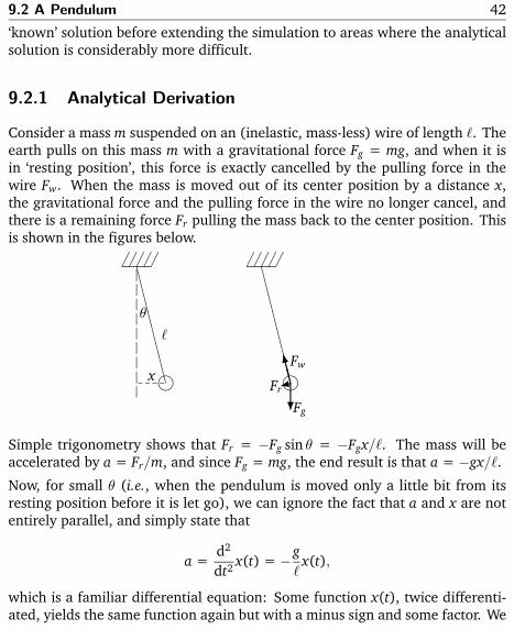
9.2.1 Analytical Derivation

Consider a mass m suspended on an (inelastic, mass- less) wire of length `. Theearth pulls on this mass m with a gravitational force Fg = mg, and when it isin ‘resting position’, this force is exactly cancelled by the pulling force in thewire Fw. When the mass is moved out of its center position by a distance x,the gravitational force and the pulling force in the wire no longer cancel, andthere is a remaining force Fr pulling the mass back to the center position. Thisis shown in the figures below.

iCCCCCCCC

��

x

θ

`

iCCCCCCCC

��

?

CCO9.

Fg

Fw

Fr

Simple trigonometry shows that Fr = −Fg sin θ = −Fgx/`. The mass will beaccelerated by a = Fr/m, and since Fg = mg, the end result is that a = −gx/`.

Now, for small θ (i.e., when the pendulum is moved only a little bit from itsresting position before it is let go), we can ignore the fact that a and x are notentirely parallel, and simply state that

a =d2

dt2 x(t) = −g`

x(t),

which is a familiar differential equation: Some function x(t), twice differenti-ated, yields the same function again but with a minus sign and some factor. We

9.2 A Pendulum 43

know the solution to such a differential equation: the sine (or cosine) function.It is more natural in this case to take the cosine, since at t = 0 we are releasingthe pendulum from a nonzero starting position x0:

x(t) = x0 cos(√

g`

t).

It is usually surprising to physics students when they first find out that the massof the pendulum has no influence on its frequency (which is 1

2π

√g/`), nor does

its initial position x0.

9.2.2 Numerical Simulation

We will characterize the pendulum by its position x and its velocity v (stillpretending that the problem is essential one- dimensional). To visualize theposition of the pendulum, we will use some crude graphics:void print_pos(double x){

int i;

if (x > 39 || x < -39)return; /* position doesn’t fit on screen */

for (i = 0; i < 40 + x; ++i)printf(" ");

printf("*");}

Assuming a screen width of 80 columns, this routine prints an asterisk at theposition of the pendulum (so we are limited to positions ranging from −39 to39, putting the ‘resting position’ in the middle of a line). Note that the functiondoes not print a ‘newline’ character (\n) after the asterisk, which you mighthave expected – we’ll see why below.The ‘body’ of the simulation consists of an endless loop which uses the functionabove to print out the current position of the pendulum and then updates itsposition and velocity:

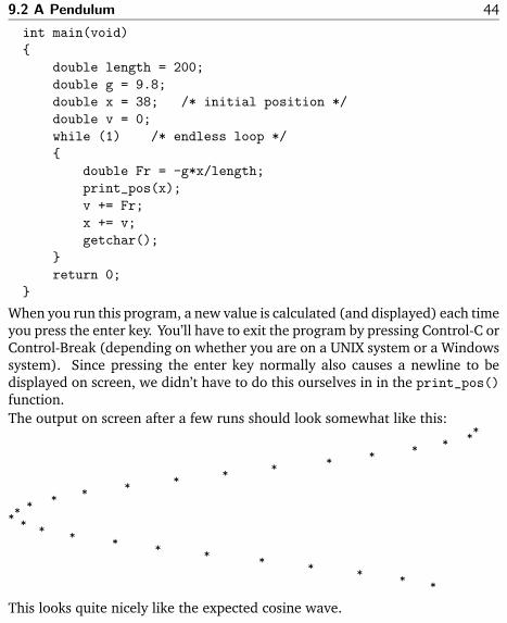
9.2 A Pendulum 44

int main(void){

double length = 200;double g = 9.8;double x = 38; /* initial position */double v = 0;while (1) /* endless loop */{

double Fr = -g*x/length;print_pos(x);v += Fr;x += v;getchar();

}return 0;

}

When you run this program, a new value is calculated (and displayed) each timeyou press the enter key. You’ll have to exit the program by pressing Control- C orControl- Break (depending on whether you are on a UNIX system or a Windowssystem). Since pressing the enter key normally also causes a newline to bedisplayed on screen, we didn’t have to do this ourselves in in the print_pos()function.The output on screen after a few runs should look somewhat like this:

**

**

**

**

**

**

**

**

**

**

**

**

**

This looks quite nicely like the expected cosine wave.

9.2 A Pendulum 45

9.2.3 Extending the Simulation

In the current model, the pendulum will keep swinging forever. In reality, thisis not so, and that is mainly due to friction of the mass as it passes throughthe air surrounding it.1 Therefore, let’s extend our model of the pendulum toinclude friction.

The mass at the end of the pendulum experiences a frictional force which isproportional to its velocity squared:

Ff =12

Cf Aρv2

where Cf is a constant depending on the shape of the object (the factor cardesigners try to get as low as possible), A is its area perpendicular to its directionof movement, and ρ the density of the medium the element is passing through.For our purposes, we can simplify this by combining all the constants:

Ff = Cv2

where C becomes another parameter of our model.

Now, we modify the expression calculating the acceleration by subtracting thefrictional force from the force exerted by the neighboring elements, and usingthis new resulting force instead:

double Fr = -g*x/length;double Ff = C*fabs(v)*v;double Ft = Fr - Ff;v += Ft;

The function fabs() returns the absolute value of its double argument. It ispart of the standard C library and can be used by including math.h. We’ve seenhow such a function could be implemented in §4.1.1This is not the only reason; a pendulum in vacuum still doesn’t keep swinging forever as it losesenergy due to internal friction as well. We will ignore this effect because it is much smaller thanthe air friction.

9.3 Random Values 46

We use this function because otherwise the resulting friction force would alwaysbe positive, in which case negative velocities (i.e., the pendulum moving ‘to theleft’ in our case) would experience an extra acceleration due to friction, insteadof a deceleration.

Setting C to about 0.02 gives a nice ‘dampening’ effect.

Before moving on to the next section, it is probably a good idea to take a lookat the first few exercises at the end of this chapter. Especially question 9.4 isimportant, since it deals with an important limitation of numerical simulations.

9.3 Random Values

In §3.6, an example was given of a function with a return value but without anyparameters. The example there was a random() function, and such a functionexists indeed. The function rand() returns a (pseudo) random integer valuebetween 0 and RAND_MAX (the definition of RAND_MAX is in stdlib.h). Of course,it is impossible to ‘calculate’ a random value, so this is pseudo random: makingclever use of the characteristics of the way numbers are handled in computers,including their overflow behavior, the result of successive calls to rand() are aseries of numbers which are in principle deterministic, but which appear to berandom. For real random values, there should be a hardware device connectedto the computer which delivers the values. You can even order CD- ROMscontaining millions of random values, which were taken from physical randomgenerators. For many purposes, however, pseudo- random values suffice.

Often, it is easier to deal with floating- point random values in the interval[0,1); for this, you can use the macro2

#define frand() (rand()/((double)RAND_MAX + 1))

We will use this function to simulate a ‘marble board’: Take a wooden boardand hammer in nails in the shape of a triangle, with one nail at the top, two on2In the original K&R book, this macro is defined slightly different, but the version presented hereworks also on systems where RAND MAX is equal to INT MAX.


the second row, three on the third, etc. (see the figure on the next page). Then,drop a series of marbles from above onto the topmost nail. Each marble willbounce on the topmost nail, either fall to the left or the right of it, then bounceon one of the nails on the second row, bounce to its left or its right again, etc.When it finally reaches the bottom of the board, each marble has made left orright bounces as many times as there are rows in the board.Given enough marbles and a big enough board, the resulting positions at whichthe marbles drop off the board at the bottom form a Gaussian distribution: If thenails are placed at the exact right positions, the chances of bouncing either leftor right are equal, and the chances of ending up near the middle of the board,after an approximately equal number of ‘left bounces’ and ‘right bounces’, aremuch greater than the chances of making only left bounces and ending up atthe far left of the board, or only right bounces and ending up at the far right.This is used in several games of chance, of which the ‘pachinko’ variety is verypopular in Japan.The figure below page shows a ‘marble board’ with 36 nails, and one possibletrajectory of a marble exiting the board in the middle.

rr rr r rr r r rr r r r rr r r r r rr r r r r r rr r r r r r r r

?

?The way we will simulate this is by virtually dropping marbles, making a seriesof ‘left- right’ decisions using the frand() macro we have just seen, and noting


the current position as we go. We will use a similar trick to draw the resultingdistribution on the screen as we used in the pendulum simulation of the previoussection. We will place a virtual row of ‘bins’ below the virtual marble boardin which each dropped marble ends up, by increasing the value in in an intarray corresponding to the ‘bin’ the marble ends up in, and we will use a (largeenough) number of experiments to build up the probability distribution.

First, let’s set up the distribution to be all- zero using a fixed number of ‘bins’.This number is a measure of the size of the marble board, and it is a parameterof our simulation. Since we will use a similar trick to display the resultingdistribution as we did in the pendulum example in the previous section, we’llpick a number which nicely fills one screen- full.

#include <stdio.h>#include <stdlib.h>

#define BINS 24#define N_EXPERIMENTS 400


void draw_distribution(int distribution[], int size){

int i, j;for (i = 0; i < size; i++){

for (j = 0; j < distribution[i]; j++)printf("*");

printf("\n");}

}

int main(void){

int distribution[BINS];int i;


/* clear the initial distribution */for (i = 0; i < BINS; i++)

distribution[i] = 0;

/* perform the simulation a number of times */for (i = 0; i < N_EXPERIMENTS; i++){

int j = BINS; /* j tracks the current position */int k;

/* "walk" the marble board */for (k = 0; k < BINS; k++){

if (frand() < 0.5) /* flip a virtual coin */j++; /* take a right */

elsej--; /* take a left */

}

/* note where the marble exited */distribution[j/2]++;

}

draw_distribution(distribution, BINS);

return 0;}

The chances of frand() returning less than 0.5 are 50%, so we are givingequal probabilities to either a left- bounce or a right- bounce. Note that we startout with j = BINS and we increase the distribution at j/2 at the end of eachsimulation, instead of starting out at BINS/2, the ‘real’ center position, andincreasing the distribution at bin j. This is because j is either increased ordecreased at each bounce and never stays unchanged, meaning that dependingon the number of bins we use, either only the even bins or only the odd binsget filled, resulting in a distribution with ‘holes’ in it.


If you run this program, something like the following distribution should appearon your screen:

****************************************************************************************************************************************************************************************************************************************************************************************************************************************************************************************************************

This approaches the familiar bell- shaped Gaussian distribution (tipped on itsside). However, if you run the program again and again, you may noticesomething interesting: You get the same curve each time! How is this possible,given that the decisions are supposed to be random?

The reason is that the rand() function returns pseudo- random numbers, aswas mentioned at the start of this section. The algorithm behind rand()works by ‘remembering’ the previous value returned, and in each successivecall performing a calculation using this number which causes an overflow, sothat the resulting new number appears to be unrelated to the previous one.However, the calculations are the same each time, so if a series starts out witha certain value, called the seed of the random generator, the resulting series ofpseudo- random numbers will be identical. At each program start, the seed isreset to the same value, hence you’ll get the same random series each time yourun the program.

Sometimes this is desirable, because this way you can ‘replay’ an experiment;but in this case, we’d rather have new results each time we try the simulation.We can arrange this by setting the seed ourselves (using the srand() function).The problem is that we need to figure out a different seed each time we runthe program, so we are facing a ‘chicken- and- egg’ problem! There is no use


calculating a random value for this seed, because that random value will be thesame every time we run the program. . .

One thing which does change from run to run is the current time. Most com-puter systems have an internal clock, and C offers functions to read out itsvalue, often in the form of a single integer number representing the numberof seconds passed since the ‘beginning of time’, for example January 1st, 1970– an arbitrary choice, and not even the same one on every system, but thatdoesn’t matter as long as it is a different value each time we run the program.If we #include <time.h>, we have the function

time_t time(time_t *tp);

It returns the current time3. If tp is non- NULL, the current time is also assignedto *tp. By using this value as the seed of our random generator, we can get adifferent series each time we run the program. Simply adding

srand(time(NULL));

to the beginning of our simulation makes sure we see different distributions ateach program run, unless we run the program quicker than the granularity oftime_t. On most systems this is one second.

Incidentally, the time.h header file also makes available a whole range of othertime- related functions, including functionality to convert a time_t value to ahuman- readable ‘calendar’ string, and for dealing with time zones and daylightsaving. More information will be given in §12.3.4.

Finally, it is worth noting that many systems offer a random generator withsignificantly better statistical properties than the simple frand() macro wewere using here. For some situations, this can be important. For example, forthe simulation of this section it wouldn’t be too much of a problem if the randomgenerator had the property that every, say, tenth ‘coin flip’ would always be theopposite result of the one immediately preceding it, as long as the chances for‘heads’ or ‘tails’ would be approximately equal for the rest of the coin flips.3Officially, it may return - 1 if there is no system clock available on this particular system, but unlessyou are on a really exotic or ancient system, this is not an issue.

9.4 Percolation 52

However, you wouldn’t use such a random generator to run an online casino,because such a ‘pattern’ would soon be found out and taken advantage of.

9.4 Percolation

In this section, we will use simulations to examine a class of phenomena knownas percolation. In the most elementary sense, the problem consists of finding aset of connected locations (i.e., a pathway) through a medium. Let us start witha 2D example in which we have an equal- spaced grid. On each grid location,there can be a ‘pass- through’ or a ‘block’. The distribution of these is determinedby a single parameter: the chance of there being a ‘pass- through’ at any givenlocation. In the figure below, a small 8 × 8 grid is shown, where open circlesdenote the ‘pass- through’ locations, and closed ones denote the ‘blocks’:

yyiiyiyiiyyiiyyyiyiyyiyiyiiiyyiiiiyiyiiyyyiiyiyiyiiyyiyiyyiiiiyy

This particular grid has 31 blocks and 33 pass- throughs, so apparently the pass-throughs were distributed with approximately 50% probability. Below is thesame grid, but with a pathway shown which connects the left side of the gridto the right side:

yyiiyiyiiyyiiyyyiyiyyiyiyiiiyyiiiiyiyiiyyyiiyiyiyiiyyiyiyyiiiiyy

9.4 Percolation 53

The goal of our simulation is to find pathways like these automatically, andfigure out what the chances are of such pathways existing as a function of thedistribution of ‘pass- throughs’ in the grid. We know by common sense that apass- through distribution probability of 0 yields a zero chance of finding anypathways, and a probability of 1 gives a ‘completely open field’. What the curvein between looks like is interesting, and this is the subject of this section.

This may seem like frivolous ‘maze- solving’, but there are interesting real-world applications in which similar situations apply. For example, if the ‘pass-throughs’ represent conducting particles and the ‘blocks’ represent insulatingparticles, then simulations like these help figure out what the chances are thata certain mixture of conducting and non- conducting particles is electricallyconducting as a whole. Another example is to estimate the probability of acertain thickness of a porous, foam- like material with a certain density beingairtight.

To do the maze- solving part, we will use the recursion concept treated in §4.9along with a new ‘trick’ called backtracking.

First, we will set up the grid. We like to print out the resulting solution tothe screen, so we take a grid size which nicely matches the screen. We fill atwo- dimensional int array (see §5.4). At each grid position, a zero means ablock (or a non- conducting cell, or a piece of solid material in a foam), and a1 represents a ‘pass- through’ (or a conducting particle, or an air bubble). Wewill first look at a program generating and displaying a single grid:

#include <stdio.h>#include <stdlib.h>#include <time.h>

#define WIDTH 79#define HEIGHT 24


void draw_grid(int grid[][WIDTH]){

int i, j;

9.4 Percolation 54

for (i = 0; i < HEIGHT; i++){

for (j = 0; j < WIDTH; j++){

if (grid[i][j] == 0)printf(" ");

elseprintf(".");

}printf("\n");

}}

int main(int argc, char *argv[]){

int grid[HEIGHT][WIDTH];int i, j;double chance = 0.5;if (argc == 2)

chance = atof(argv[1]);srand(time(NULL));for (i = 0; i < HEIGHT; i++){

for (j = 0; j < WIDTH; j++){

if (frand() < chance)grid[i][j] = 1;

elsegrid[i][j] = 0;

}}draw_grid(grid);return 0;

}

9.4 Percolation 55

If you run this program a few times with different probability values, you willget a feeling for the ‘density’ of such grids.

Incidentally, the loop filling the grid could have been written a lot more compact(and cryptic) as

for (i = 0; i < HEIGHT; i++)for (j = 0; j < WIDTH; j++)

grid[i][j] = (frand() < chance);

See §4.3 about boolean expressions if this doesn’t make sense straight away.

Now for the ‘meat’ of our simulation: automatically finding out whether thereis any pathway from the left side of the grid to the right side.

Looking at this problem with recursion in mind, the notion of a ‘pathway to theright side’ can be formulated a little differently: A certain grid point is part of apathway to the right side if at least one of its neighboring grid points is part of apathway. In other words: You can reach the other side of the grid from a certainpoint if you can reach the other side of the grid from one of its neighbors.

Therefore, we will simply walk along all points on the left side of the grid, anddetermine whether any of these fulfills the descriptions above. If so, we canstop: we needn’t find all pathways nor the shortest.

Let us construct the recursive function to do this ‘pathway check’. First, let’sdefine its return value: It should be zero if it’s not part of a pathway, and oneif it is:

int percolate(int grid[][WIDTH], int i, int j){

if (i < 0 || j < 0 || i >= HEIGHT)return 0; /* invalid position: fell off the grid */

if (i >= WIDTH)return 1; /* we have reached the right side! */

if (grid[i][j] == 0)return 0; /* we ran into a block */

/* check whether our neighbors are part of a pathway */

9.4 Percolation 56

if (percolate(grid, i, j + 1) /* right neighbor? */|| percolate(grid, i, j - 1) /* or the left one? */|| percolate(grid, i + 1, j) /* or below us? */|| percolate(grid, i - 1, j)) /* or above? */

return 1; /* If so, we’re part of the pathway too *//* otherwise, this is a dead end */return 0;

}

It may be strange to see four recursive calls of the same function, but you arefree to make as many as you like. It can be mind- boggling if you try to performthis ‘in your head’, but the compiler does a good job of it so you don’t have to.

The bottom part of the function performs the test we described above: If wearen’t on a block, and one of our neighboring grid points is part of a pathway,then we are part of a pathway too. The top part of the function makes surewe don’t run off the grid, and takes care of stopping the recursion when wereach the other side of the grid. Be sure to let this function ‘sink in’ for awhile, perhaps using the example grid presented earlier in this section, and seewhether you can develop a good feeling for how this algorithm works.

It may be helpful to keep the following analogy in mind. Suppose you aredropped at the entrance of a maze, and your task is to say whether this mazehas an exit. Further suppose that you have the capability of splitting off identicalclones of yourself. One way to solve your task is to split off a clone of yourselfand send him into the maze, with simple instructions:

1. At each junction in the maze, pick one corridor for yourself and sendclones of yourself into the others, giving each of these clones this exactlist of instructions

2. report back at the previous junction when you either run into a dead endor find the exit

3. when you arrive back at the previous junction, wait for all your clonesto arrive there too and ‘re- join’ with them into a single entity again,remembering whether you or any of your clones has found the exit, andfinally

4. report back at the previous junction.

9.4 Percolation 57

When a clone returns to his spawning point, he can either report that “one ofthe paths I just came from reaches an exit” or “none of the paths I just camefrom reaches an exit”. Finally, the first clone you split off comes walking out ofthe maze and reports to you whether any of his clones has found an exit.

With the help of the analogy, perhaps you can also find the fatal flaw in thisalgorithm before reading the next paragraph.

This algorithm will quickly end up in infinite recursion. Why? Because a clonecannot determine whether a certain maze junction has been visited before. Oneof the clones is bound to reach a junction already visited, split off new clones,and send them off following ‘older clones’. In fact, one of them will run into thevery corridor his ‘parent’ just came from! Clearly, recursion alone isn’t enoughto solve this task.

Enter backtracking. This is the computational equivalent of the fairy tale ofLittle Thumbkin, leaving a trail of bread crumbs on his way through the forest.What we have to do is mark the grid points we’ve already visited. Below is amodified version of the percolate() function which does just that.

int percolate(int grid[][WIDTH], int i, int j){

if (i < 0 || j < 0 || i >= HEIGHT)return 0;

if (j >= WIDTH)return 1;

if (grid[i][j] == 0)return 0;

/* have we visited this point before? */if (grid[i][j] > 1)

return 0; /* in that case, don’t bother continuing */

/* Mark this grid as visited */grid[i][j] = 2;

if (percolate(grid, i, j + 1)

9.4 Percolation 58

|| percolate(grid, i, j - 1)|| percolate(grid, i + 1, j)|| percolate(grid, i - 1, j)){

/* mark as visited AND part of a pathway */grid[i][j] = 3;return 1;

}

return 0;}

We need to modify the draw_grid() function a bit to deal with these ‘marked’grid points:

void draw_grid(int grid[][WIDTH]){

int i, j;for (i = 0; i < HEIGHT; i++){

for (j = 0; j < WIDTH; j++){

if (grid[i][j] == 1 || grid[i][j] == 2)printf(".");

else if (grid[i][j] == 3)printf("*");

elseprintf(" ");

}printf("\n");

}}

Below is a typical output of the program with a pass- through density of 0.7:

9.4 Percolation 59

. .... .......... .... .... ... . ... ...... . .... ....... .. . ..... . ......... ... .. ....... . ... ......... .... . ..... .. . .... .. ... .......... . .... .... . . ..... .. ............. .. ........... . ... . ... ..

. . . ......... ... .... .. . .......... ....... ..... . ..... . . .. ..... .. . . ... .. .. . ... .. . . . .. . . . .. ... .......... .

********* . ... ..... . .. ... .... ............ . .. .. .. ... .. ... .... ... ..**. . . ...... ...... .... ........... .. . . .. ..... . . ... .......... * ..... . .. . .... .. ...... . ******* ... ........... .....

......** . . . . .. .. ...... ... ... .. ..*** . **** ......... .. . .... . ..****** ... ... ............. ... .. ***. .. ************* . ....

.. ... .. . ..** .. ... . ... . .... ... .... **** .. .. ... . ** .*****

..... .**** ****. .... .. ....... ......... ... *** .... *********** * .

. . .. ** *** .. . ..... . ............. .... . .** . .. .** ........*.. .

.. .... *. .. . .... .. ....... ... . . . ...*** . .. . .** .. . ..*** .

........ * . .. . .. . . .. . ...... .........*** ...... *. .. .. . *** . .. . ....****** .. ........ .. . . .... ****** .. . ... ** .... *******.. .

... ........ * .. . . ....********** . ** ... .. .. . . .****. * .. .. ..

... ...... ...***. .... .. . **** ....***** ... . ......... ** . **. . ......... .. ... * ... .....***** ...... ... . .. ... . ****. ..* . ........... . ...** ........** **** ............. ... . ... .*** .. ***.. .......... ...... ...** ...... **** **. .. ... . .. ... .. ...** ... ** .. .. .

. .. .... .... .*********** ** .......... ...... . . . ..*********. . . .

............. ........ ...**** .... . ... . .... ........ ... . .. .......... . ....... .. .... ..... . ...... .. ....... .. .... . ... . ............. .. ... .. ... ......... .... . . ... ... . . . . .. .. .. ..... ..

Note that the code above simply finds the first pathway, not necessarily theshortest. For our current experiments, we aren’t particularly interested in thelength of the pathway; just in whether there is one.

There are several questions and exercises at the end of this chapter, startingwith exercise 9.7, in which the simulation of this section is used to examinesome interesting properties of these grids.

As a final note: we are using an int array for the grid, and this is a bit ‘overkill’since we only use four different values for each grid position (out of the fourbillion values available for an int). For the grid size we’ve been considering, thisis not an issue. However, on many systems the amount of memory availableon the stack is limited to a much smaller size than heap memory (memoryavailable through malloc(), see page 147). If you are running the simulationwith larger grids, or extend it to examine three- dimensional grids, you may geta compiler error that the grid array is getting too big for the stack. In thatcase, you could modify it to use chars instead of ints, which will buy you afactor of four. Ultimately, you will need to modify the program to work with

9.5 Synopsis 60

dynamically allocated memory (see §5.7).

9.5 Synopsis

This chapter presented several ‘real- world’ examples of simulations and com-puter experiments. In all cases, it is important to find a mapping of a real- worldsituation to a model which is suitable for computer simulations, i.e., a discretemodel. It is important to realize that this discretization step has some implica-tions to the reliability of the simulation, and there is often a tradeoff betweenspeed and accuracy. For an accurate simulation, you’d rather take very smalldiscretization steps, requiring many iterations of the algorithm, and which mayget ‘stuck’ due to ‘underflow’: The differences in each step are so small thatthey get lost in the limited precision of the computer. For fast results you woulduse large discretization steps, with the risk of ‘overshoot’ where the simulationmay ‘explode’.

In many simulations, random behavior is required. Since ‘generating randomnumbers on a computer’ is a contradiction in terms, you normally have to settlefor pseudo- random behavior. The computer can generate a series of numberswhich appear to be random; the quality of the random generator is measuredby how easy it is to spot certain ‘patterns’ in the sequence of numbers.

A certain class of problems can be tackled by using ‘maze- solving’ algorithms.Here, an important extension to recursion is backtracking, in which the recursivesearch for solutions is augmented by marking which solutions have already beenexamined, and ‘reversing the steps’ once it turns out that a certain path doesn’tlead to a solution.

A simulation using only ‘first principles’, is called an ab initio experiment. Itcan be dangerous to interpret the results of such simulations because you mustbe sure you haven’t left out any important effects. In a ‘real’ experiment, youusually assume that the measurements are right – if they don’t stroke with yourhypothesis, it is quite likely that the hypothesis is incomplete. In a computersimulation, there may be other effects to deal with, like limited precision,overflow or underflow, or even simple miscalculations.

9.6 Other Languages 61

9.6 Other Languages

C was not designed with scientific simulations in mind, but the language doeslend itself quite nicely to such experiments. For some experiments, an object-oriented language (see §6.5) might be more suitable, because you can directlymap concepts of the real- world situation to classes of objects in the language.

Most languages offer sufficient mathematics support for most experiments, andmost support recursion (and thus backtracking).

Traditionally, most ‘scientific’ programs are written in FORTRAN (which is olderthan C). In fact, its name comes from FORmula TRANslator, and it was specif-ically designed so that scientists could write programs which looked more‘mathematical’ instead of using the machine language of a particular machine(see §1).

Because FORTRAN has been the ‘language of choice’ for scientists for severaldecades, there exists an enormous amount of ‘mature’ (i.e., highly optimizedand reliable) code in so- called libraries (see chapters 10 and 12), but it is oftenpossible to call functions from these libraries from your C programs.


9.1 In the pendulum simulation of §9.2, determine the period of the pendulum,either by simply counting the number of times you need to press the enter keybefore the pendulum reaches its original position again, or by modifying theprogram to keep track of the maximum position. How does it compare to thetheoretical value? Also modify the length of the wire and see whether theresulting frequencies correspond to the theory.

9.2 Determine the effect of the ‘friction term’ on the frequency of the pendulum.

9.3 Varying the friction constant C in the pendulum simulation determines howquickly the pendulum is at rest again. When C is very low, the pendulum will


not experience much friction and keep swinging for a long time; When C isabove a certain value, the pendulum will not even swing at all (i.e., it slowlyapproaches its resting position and never swings to the other side). This wouldcorrespond to a pendulum placed in a container full of syrup or some otherviscous liquid. When C has the smallest value for which the pendulum justdoesn’t swing anymore, the system is said to be critically dampened. Determinethis value of C.

9.4 The constant g used in the pendulum simulation is only valid here on Earth.On different planets, there would be a different g. Change the value of g tobe ten times as big and see what influence that has on the frequency of thependulum. Then, change it to be a hundred times as big (to simulate, say, apendulum near a heavy star). What happens? Can you explain? How couldyou modify the code to handle extreme gravity like this?

9.5 ? Making the length of the pendulum comparable to the initial position x0

will render the derivation invalid, but the code of the simulation does not takethis into account. Modify the simulation so that it takes vertical accelerationinto account as well (i.e., distinguish between vx and vy) and keep track of thevertical position of the mass. You will need to take centripetal acceleration intoaccount (ac = v2/r), or the pendulum will keep ‘falling down’. You may noticethat it is very hard to get good results with your simulation, because the errorsmade in each step keep adding up, rendering the simulation useless.

9.6 In the marble board simulation of §9.3, modify the left- right decision cri-terion to give different chances for left and right (i.e., use a ‘loaded die’) andobserve how this changes the resulting distribution.

9.7 The first thing to examine with the ‘percolation grids’ of §9.4 is the prob-ability to find a pathway as a function of the probability used to distribute‘pass- throughs’ and ‘blocks’. Examine all such distribution probabilities from 0to 1 in increments of 0.05, perform several simulations at each probability, andplot the probability of finding a pathway. You will quickly find out that there isa ‘critical density’ around which the pathway probability rises steeply. What isthis ‘critical density’ for the grid size used in the examples?


9.8 Obviously, the grid size is an important factor too. Examine the effect ofgrid dimensions on the ‘critical density’.

9.9 In the clone analogy, one could argue that it would be much easier to simplyleave one clone at each junction, who ‘remembers’ where he came from, andonly send off his clones in the other directions. Modify the program to be morelike this. Can you get it simpler this way?

9.10 ? Modify the pathway- finding algorithm to find the shortest pathwaythrough a given grid. Given this modified algorithm, plot the average pathwaylength against the pass- through probability, not counting simulations whichcouldn’t find a pathway at all. Hint: the percolate() function as it is nowonly returns whether there was a pathway in this direction. Can you modify itto return the number of steps needed to reach it? At each grid point, comparethe return values of percolate() and let the shortest nonzero value win. Oneis added (for the current grid point) and the result returned again.

computer programming - curly-brace.com · computer programming an introduction for the...

Documents