1

Computer Networking

Lent Term M/W/F 11-middayLT1 in Gates Building

Slide Set 3

Andrew W. Mooreandrew.moore@cl.cam.ac.uk

January 2013

2

Topic 3: The Data Link LayerOur goals: • understand principles behind data link layer services:

(these are methods & mechanisms in your networking toolbox)– error detection, correction– sharing a broadcast channel: multiple access– link layer addressing– reliable data transfer, flow control: \

– instantiation and implementation of various link layer technologies

– Wired Ethernet (aka 802.3)– Wireless Ethernet (aka 802.11 WiFi)

3

Link Layer: IntroductionSome terminology:• hosts and routers are nodes• communication channels that

connect adjacent nodes along communication path are links– wired links– wireless links– LANs

• layer-2 packet is a frame, encapsulates datagram

data-link layer has responsibility of transferring datagram from one node to adjacent node over a link

4

Link Layer (Channel) Services• framing, link access:

– encapsulate datagram into frame, adding header, trailer– channel access if shared medium– “MAC” addresses used in frame headers to identify source, dest

• different from IP address!• reliable delivery between adjacent nodes

– we learned how to do this already (chapter 3)!– seldom used on low bit-error link (fiber, some twisted pair)– wireless links: high error rates

• Q: why both link-level and end-end reliability?

5

Link Layer (Channel) Services - 2

• flow control: – pacing between adjacent sending and receiving nodes

• error detection: – errors caused by signal attenuation, noise. – receiver detects presence of errors:

• signals sender for retransmission or drops frame

• error correction: – receiver identifies and corrects bit error(s) without resorting to

retransmission

• half-duplex and full-duplex– with half duplex, nodes at both ends of link can transmit, but not at same

time

6

Where is the link layer implemented?

• in each and every host• link layer implemented in

“adaptor” (aka network interface card NIC)– Ethernet card, PCMCI card,

802.11 card– implements link, physical layer

• attaches into host’s system buses

• combination of hardware, software, firmware

controller

physicaltransmission

cpu memory

host bus (e.g., PCI)

network adaptercard

host schematic

applicationtransportnetwork

link

linkphysical

7

Adaptors Communicating

• sending side:– encapsulates datagram in frame– encodes data for the physical

layer– adds error checking bits, provide

reliability, flow control, etc.

• receiving side– decodes data from the physical

layer– looks for errors, provide

reliability, flow control, etc– extracts datagram, passes to

upper layer at receiving side

controller controller

sending host receiving host

datagram datagram

datagram

frame

8

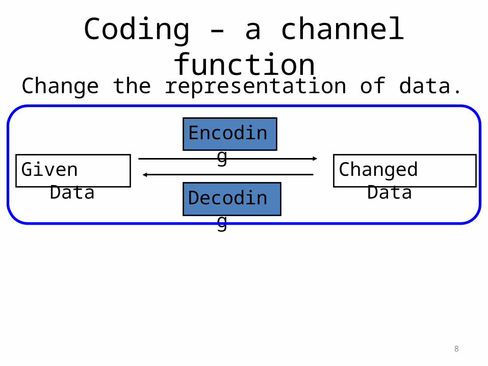
Coding – a channel functionChange the representation of data.

Given Data Changed Data

Encoding

Decoding

9

MyPasswd

AA$$$$ff

MyPasswd

AA$$$$ff

AA$$$$ffff AA$$$$ffff

10

CodingChange the representation of data.

Given Data Changed Data

Encoding

Decoding

1. Encryption: MyPasswd <-> AA$$$$ff2. Error Detection: AA$$$$ff <-> AA$$$$ffff3. Compression: AA$$$$ffff <-> A2$4f44. Analog: A2$4f4 <->

11

0 1 1 1 1 10000

0 1 1 1 1 10000

0 1 1 1 1 10000

Non-Return-to-Zero (NRZ)

Non-Return-to-Zero-Mark (NRZM) 1 = transition 0 = no transition

Non-Return-to-Zero Inverted (NRZI) (note transitions on the 1)

Line Coding Exampleswhere Baud=bit-rate

12

0 1 0 1 1 11000

Non-Return-to-Zero (NRZ) (Baud = bit-rate)

Manchester example (Baud = 2 x bit-rate)

Clock

Line Coding Examples - II

0 1 0 1 1 11000

0 1 0 1 1 11000

Quad-level code (2 x Baud = bit-rate)

Clock

13

0 1 0 1 1 11000

Line Coding Examples - III

Name 4b 5b Description

0 0000 11110 hex data 0

1 0001 01001 hex data 1

2 0010 10100 hex data 2

3 0011 10101 hex data 3

4 0100 01010 hex data 4

5 0101 01011 hex data 5

6 0110 01110 hex data 6

7 0111 01111 hex data 7

8 1000 10010 hex data 8

9 1001 10011 hex data 9

A 1010 10110 hex data A

B 1011 10111 hex data B

C 1100 11010 hex data C

D 1101 11011 hex data D

E 1110 11100 hex data E

F 1111 11101 hex data F

Name 4b 5b Description

Q -NONE- 00000 Quiet

I -NONE- 11111 Idle

J -NONE- 11000 SSD #1

K -NONE- 10001 SSD #2

T -NONE- 01101 ESD #1

R -NONE- 00111 ESD #2

H -NONE- 00100 Halt

0 1 1 0 0 11010

Block coding transfers data with a fixedoverhead: 20% less information per Baud in the case of 4B/5B

So to send data at 100Mbps; the line rate(the Baud rate) must be 125Mbps.

1Gbps uses an 8b/10b codec; encoding entire bytes at a time but with 25% overhead

Data to send

Line-(Wire) representation

14

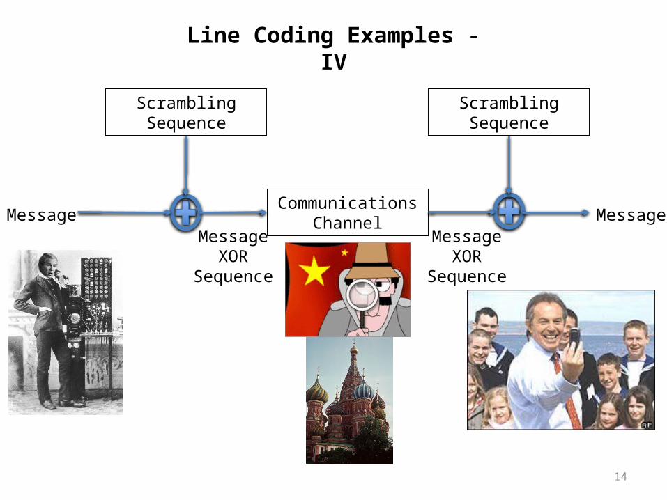
Line Coding Examples - IV

ScramblingSequence

ScramblingSequence

CommunicationsChannelMessage Message

MessageXOR

Sequence

MessageXOR

Sequence

15

Line Coding Examples - V

ScramblingSequence

ScramblingSequence

CommunicationsChannelMessage Message

MessageXOR

Sequence

MessageXOR

Sequence

δ δ δ δ δ

e.g. (Self-synchronizing) scrambler

16

Line Coding Examples – VI(Hybrid)

δ δ δ δ δδ δ δ δ δ

…100111101101010001000101100111010001010010110101001001110101110100…

Inserted bits marking “start of frame/block/sequence”

…10011110110101000101000101100111010001010010110101001001110101110100…

Scramble / Transmit / Unscramble

…0100010110011101000101001011010100100111010111010010010111011101111000…

Identify (and remove) “start of frame/block/sequence”This gives you the Byte-delineations for free

64b/66b combines a scrambler and a framer. The start of frame is a pair of bits 01 or 10: 01 means “this frame is data” 10 means “this frame contains data and control” – control could be configuration information, length of encoded data or simply “this line is idle” (no data at all)

17

?CLASSIFIED:

TOP SECRET

NO FORNAT

18

Multiple Access Mechanisms

Each dimension is orthogonal (so may be trivially combined)There are other dimensions too; can you think of them?

19

20

21

22

Code Division Multiple Access (CDMA)

• used in several wireless broadcast channels (cellular, satellite, etc) standards

• unique “code” assigned to each user; i.e., code set partitioning

• all users share same frequency, but each user has own “chipping” sequence (i.e., code) to encode data

• encoded signal = (original data) X (chipping sequence)

• decoding: inner-product of encoded signal and chipping sequence

• allows multiple users to “coexist” and transmit simultaneously with minimal interference (if codes are “orthogonal”)

23

CDMA Encode/Decode

slot 1 slot 0

d1 = -1

1 1 1 1

1- 1- 1- 1-

Zi,m= di.cmd0 = 1

1 1 1 1

1- 1- 1- 1-

1 1 1 1

1- 1- 1- 1-

1 1 11

1-1- 1- 1-

slot 0channeloutput

slot 1channeloutput

channel output Zi,m

senderadds code code

databits

slot 1 slot 0

d1 = -1d0 = 1

1 1 1 1

1- 1- 1- 1-

1 1 1 1

1- 1- 1- 1-

1 1 1 1

1- 1- 1- 1-

1 1 11

1-1- 1- 1-

slot 0channeloutput

slot 1channeloutputreceiver

removes code

code

receivedinput

Di = S Zi,m.cmm=1

M

M

24

CDMA: two-sender interference

Each sender adds a uniquecode

senderremovesits uniquecode

25

Coding Examples summary

• Common Wired coding– Block codecs: table-lookups

• fixed overhead, inline control signals

– Scramblers: shift registers• overhead free

Like earlier coding schemes and error correction/detection; you can combine these

– e.g, 10Gb/s Ethernet may use a hybrid

CDMA (Code Division Multiple Access)– coping intelligently with competing sources– Mobile phones

26

How to use coding to deal with errors in data communication?

Noise

0000 0001

Basic Idea : 1. Add additional information to a message. 2. Detect an error and re-send a message. Or, fix an error in the received message.

0000 0000

Error Detection and Correction

27

How to use coding to deal with errors in data communication?

Noise

0000 0000

Basic Idea : 1. Add additional information to a message. 2. Detect an error and re-send a message. Or, fix an error in the received message.

0000 0000

Error Detection and Correction

28

Error DetectionEDC= Error Detection and Correction bits (redundancy = overhead)D = Data protected by error checking, may include header fields

• Error detection not 100% reliable!• protocol may miss some errors, but rarely• larger EDC field yields better detection and correction

otherwise

29

Error Detection CodeSender: Y = generateCheckBit(X);send(XY);

Receiver:

receive(X1Y1);Y2=generateCheckBit(X1);if (Y1 != Y2) ERROR;else NOERROR

Noise

==

30

Error Detection Code: ParityAdd one bit, such that the number of 1’s is even.

Noise

0000 0

0001 1

1001 0

0001 0

0001 1

1111 0

Problem: This simple parity cannot detect two-bit errors.

31

Parity CheckingSingle Bit Parity:Detect single bit errors

Two Dimensional Bit Parity:Detect and correct single bit errors

0 0

32

Internet checksum

Sender:• treat segment contents as

sequence of 1bit integers• checksum: addition (1’s

complement sum) of segment contents

• sender puts checksum value into UDP checksum field

Receiver:• compute checksum of received

segment• check if computed checksum

equals checksum field value:– NO - error detected– YES - no error detected. But

maybe errors nonetheless?

Goal: detect “errors” (e.g., flipped bits) in transmitted packet (note: used at transport layer only)

33

Error Detection Code: CRC

• CRC means “Cyclic Redundancy Check”.• More powerful than parity.

• It can detect various kinds of errors, including 2-bit errors.

• More complex: multiplication, binary division.• Parameterized by n-bit divisor P.

• Example: 3-bit divisor 101.• Choosing good P is crucial.

34

CRC with 3-bit Divisor 101

Multiplication by 23

D2 = D * 23

Binary Division by 101CheckBit = (D2) rem (101)

1001

1001000

11

Add three 0’s at the end Kurose p478 §5.2.3Peterson p97 §2.4.3

00

1111000

1111

0

0

CRC Paritysame check bits from Parity,but different ones from CRC

35

The divisor (G) – Secret sauce of CRC

• If the divisor were 100, instead of 101, data 1111 and 1001 would give the same check bit 00.

• Mathematical analysis about the divisor:– Last bit should be 1.– Should contain at least two 1’s.– Should be divisible by 11.

• ATM, HDLC, Ethernet each use a CRC with well-chosen fixed divisors

Divisor analysis keeps mathematicians in jobs(a branch of pure math: combinatorial mathematics)

36

Checksumming: Cyclic Redundancy Checkrecap

• view data bits, D, as a binary number• choose r+1 bit pattern (generator), G • goal: choose r CRC bits, R, such that

– <D,R> exactly divisible by G (modulo 2) – receiver knows G, divides <D,R> by G. If non-zero remainder: error

detected!– can detect all burst errors less than r+1 bits

• widely used in practice (Ethernet, 802.11 WiFi, ATM)

37

CRC Another Example – this time with long division

Want:

D.2r XOR R = nPequivalently:

D.2r = nP XOR R equivalently: if we divide D.2r by P,

want remainder R

R = remainder[ ]D.2r

P

P

FYI: in K&R P is called the Generator: G

38

Error Detection Code becomes….Sender: Y = generateCheckBit(X);send(XY);

Receiver:

receive(X1Y1);Y2=generateCheckBit(X1);if (Y1 != Y2) ERROR;else NOERROR

Noise

==

39

Forward Error Correction (FEC)

Sender: Y = generateCheckBit(X);send(XY);

Noise

Receiver:

receive(X1Y1);Y2=generateCheckBit(X1);if (Y1 != Y2) FIXERROR(X1Y1);else NOERROR

!=

40

Forward Error Correction (FEC)

Sender: Y = generateCheckBit(X);send(XY);

Noise

==

Receiver:

receive(X1Y1);Y2=generateCheckBit(X1);if (Y1 != Y2) FIXERROR(X1Y1);else NOERROR

41

Basic Idea of Forward Error Correction

Replace erroneous data by its “closest” error-free data.

00 000

01 011

10 101

11 110

01 00011 101

10 110

Good

GoodGood

Good

BadBad Bad

3

4

2

1

42

Error Detection vs Correction

Error Correction:• Cons: More check bits. False recovery.• Pros: No need to re-send.Error Detection:• Cons: Need to re-send. • Pros: Less check bits. Usage:• Correction: A lot of noise. Expensive to re-send.• Detection: Less noise. Easy to re-send.• Can be used together.

43

Multiple Access Links and Protocols

Two types of “links”:• point-to-point

– point-to-point link between Ethernet switch and host

• broadcast (shared wire or medium)– old-fashioned wired Ethernet (here be dinosaurs – extinct)– upstream HFC (Hybrid Fiber-Coax – the Coax may be broadcast)– 802.11 wireless LAN

shared wire (e.g., cabled Ethernet)

shared RF (e.g., 802.11 WiFi)

shared RF(satellite)

humans at acocktail party

(shared air, acoustical)

44

Multiple Access protocols• single shared broadcast channel • two or more simultaneous transmissions by nodes:

interference – collision if node receives two or more signals at the same time

multiple access protocol• distributed algorithm that determines how nodes share

channel, i.e., determine when node can transmit• communication about channel sharing must use channel itself!

– no out-of-band channel for coordination

45

Ideal Multiple Access Protocol

Broadcast channel of rate R bps1. when one node wants to transmit, it can send at rate R2. when M nodes want to transmit, each can send at average

rate R/M3. fully decentralized:

– no special node to coordinate transmissions– no synchronization of clocks, slots

4. simple

46

MAC Protocols: a taxonomy

Three broad classes:• Channel Partitioning

– divide channel into smaller “pieces” (time slots, frequency, code)– allocate piece to node for exclusive use

• Random Access– channel not divided, allow collisions– “recover” from collisions

• “Taking turns”– nodes take turns, but nodes with more to send can take longer

turns

47

Channel Partitioning MAC protocols: TDMA(time travel warning – we mentioned this earlier)

TDMA: time division multiple access • access to channel in "rounds" • each station gets fixed length slot (length = pkt trans time)

in each round • unused slots go idle • example: station LAN, 1,3,4 have pkt, slots 2,5,6 idle

1 3 4 1 3 4

slotframe

48

Channel Partitioning MAC protocols: FDMA(time travel warning – we mentioned this earlier)

FDMA: frequency division multiple access • channel spectrum divided into frequency bands• each station assigned fixed frequency band• unused transmission time in frequency bands go idle • example: station LAN, 1,3,4 have pkt, frequency bands 2,5,6

idle

freq

uenc

y ba

nds

time

FDM cable

49

“Taking Turns” MAC protocols

channel partitioning MAC protocols:

– share channel efficiently and fairly at high load– inefficient at low load: delay in channel access, 1/N

bandwidth allocated even if only 1 active node! Random access MAC protocols

– efficient at low load: single node can fully utilize channel

– high load: collision overhead“taking turns” protocols

look for best of both worlds!

50

“Taking Turns” MAC protocolsPolling: • master node “invites”

slave nodes to transmit in turn

• typically used with “dumb” slave devices

• concerns:– polling overhead – latency– single point of failure

(master)

master

slaves

poll

data

data

51

“Taking Turns” MAC protocolsToken passing: control token passed from

one node to next sequentially.

token message concerns:

token overhead latency single point of failure (token)

concerns fixed in part by a slotted ring (many simultaneous tokens)

T

data

(nothingto send)

T

Cambridge students – this is YOUR heritageCambridge RING, Cambridge Fast RING,Cambridge Backbone RING, these things gave us ATDM (and ATM)

52

ATM

1 3 4 1 3 4

slotframe

1 3 4 11 4

ATM = Asynchronous Transfer Mode – an ugly expressionthink of it as ATDM – Asynchronous Time Division Multiplexing

That’s PACKET SWITCHING to the rest of us – just like Ethernetbut using

fixed length slots/packets/cells

Use the media when you need it, butATM had virtual circuits and these needed setup….

Worse ATM had an utterly irrational size

In TDM a sender may only use a pre-allocated slot

In ATM a sender transmits labeled cells whenever necessary

3

53

ATM Layer: ATM cell (size = best known stupid feature)

• 48-byte payload

– Why?: small payload -> short cell-creation delay for digitized voice

– halfway between 32 and 64 (compromise!)• 5-byte ATM cell header (10% of payload)

Cell header

Cell format

54

Size issues once plagued ATM- too little time to do useful work

now plague the common Internet MTU

Even jumbo grams (9kB) are argued as not big enough

Consider issues• default Ethernet CRC not robust for 9k

packets• IPv6 checksum implications

• MTU discovery ugliness• (discovering MTU is hard anyway)

• Is time-per-packet a sensible justification?

ATM – redux, the irony(a 60 second sidetrack)

None of these are the “Internet way”…(Bezerkely, 60’s, free stuff, no G-man)

• Seriously; why not?

• What’s wrong with– TDMA– FDMA– Polling– Token passing– ATM

• Turn to random access– Optimize for the common case (no collision)– Don’t avoid collisions, just recover from them….

• Sound familiar?

What could possibly go wrong….55

Management. Suites. Rules. Schedules.

Signs, signs, everywhere a sign….

56

Random Access Protocols

• When node has packet to send– transmit at full channel data rate R.– no a priori coordination among nodes

• two or more transmitting nodes ➜ “collision”,• random access MAC protocol specifies:

– how to detect collisions– how to recover from collisions (e.g., via delayed retransmissions)

• Examples of random access MAC protocols:– ALOHA and slotted ALOHA– CSMA, CSMA/CD, CSMA/CA

57

Random Access MAC Protocols

• When node has packet to send– Transmit at full channel data rate– No a priori coordination among nodes

• Two or more transmitting nodes collision– Data lost

• Random access MAC protocol specifies: – How to detect collisions– How to recover from collisions

• Examples – ALOHA and Slotted ALOHA– CSMA, CSMA/CD, CSMA/CA (wireless)

58

Key Ideas of Random Access

• Carrier sense– Listen before speaking, and don’t interrupt– Checking if someone else is already sending data– … and waiting till the other node is done

• Collision detection– If someone else starts talking at the same time, stop– Realizing when two nodes are transmitting at once– …by detecting that the data on the wire is garbled

• Randomness– Don’t start talking again right away– Waiting for a random time before trying again

59

Where it all Started: AlohaNet• Norm Abramson left

Stanford to surf• Set up first data

communication system for Hawaiian islands

• Hub at U. Hawaii, Oahu• Had two radio

channels:– Random access:

• Sites sending data– Broadcast:

• Hub rebroadcasting data

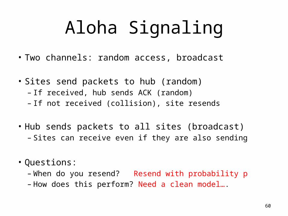
Aloha Signaling

• Two channels: random access, broadcast

• Sites send packets to hub (random)– If received, hub sends ACK (random)– If not received (collision), site resends

• Hub sends packets to all sites (broadcast)– Sites can receive even if they are also sending

• Questions:– When do you resend? Resend with probability p– How does this perform? Need a clean model….

60

61

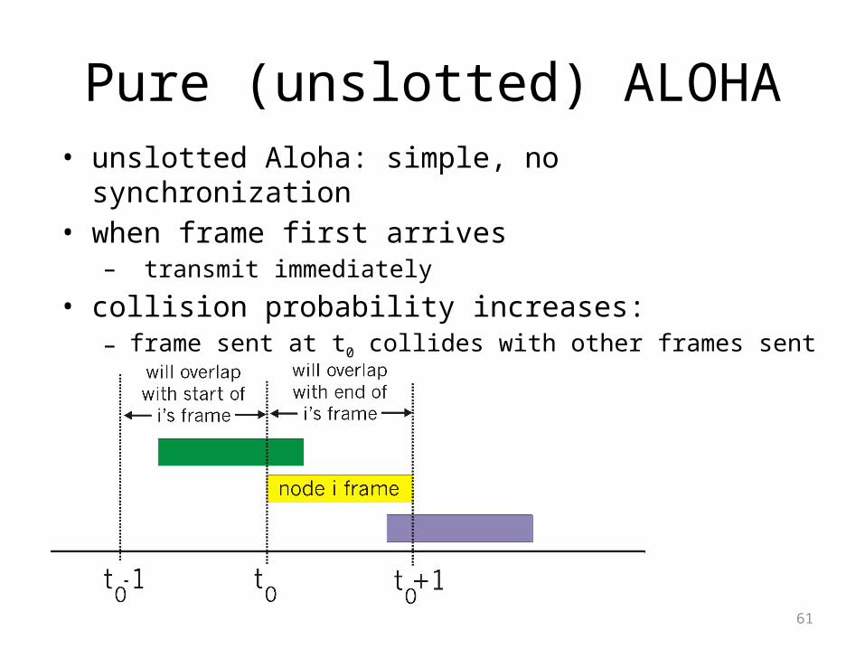
Pure (unslotted) ALOHA• unslotted Aloha: simple, no synchronization• when frame first arrives

– transmit immediately

• collision probability increases:– frame sent at t0 collides with other frames sent in [t0-1,t0+1]

62

Pure Aloha efficiency

P(success by given node) = P(node transmits) .

P(no other node transmits in [p0-1,p0] .

P(no other node transmits in [p0-1,p0]

= p . (1-p)N-1 . (1-p)N-1

= p . (1-p)2(N-1)

… choosing optimum p and then letting n -> ∞ ...

= 1/(2e) = .18

Best described as unspectacular; but better than what went before.

63

Slotted ALOHA

Assumptions• All frames same size• Time divided into equal slots (time to transmit a frame)• Nodes are synchronized• Nodes begin to transmit frames only at start of slots• If multiple nodes transmit, nodes detect collision

Operation• When node gets fresh data,

transmits in next slot• No collision: success!• Collision: node retransmits

with probability p until success

64

Slot-by-Slot Example

65

Efficiency of Slotted Aloha• Suppose N stations have packets to send

– Each transmits in slot with probability p

• Probability of successful transmission:by a particular node i: Si = p (1-p)(N-1)

by any of N nodes: S= N p (1-p)(N-1)

• What value of p maximizes prob. of success:– For fixed p, S 0 as N increases– But if p = 1/N, then S 1/e = 0.37 as N increases

• Max efficiency is only slightly greater than 1/3!

66

Pros and Cons of Slotted Aloha

Pros• Single active node can

continuously transmit at full rate of channel

• Highly decentralized: only need slot synchronization

• Simple

Cons• Wasted slots:

– Idle– Collisions

• Collisions consume entire slot

• Clock synchronization

67

Improving on Slotted Aloha

• Fewer wasted slots– Need to decrease collisions and empty slots

• Don’t waste full slots on collisions– Need to decrease time to detect collisions

• Avoid need for synchronization– Synchronization is hard to achieve

68

CSMA (Carrier Sense Multiple Access)

• CSMA: listen before transmit– If channel sensed idle: transmit entire frame– If channel sensed busy, defer transmission

• Human analogy: don’t interrupt others!

• Does this eliminate all collisions?– No, because of nonzero propagation delay

69

CSMA CollisionsPropagation delay: two nodes may not hear each other’s before sending.

Would slots hurt or help?

CSMA reduces but does not eliminate collisions

Biggest remaining problem?

Collisions still take full slot!How do you fix that?

70

CSMA/CD (Collision Detection)

• CSMA/CD: carrier sensing, deferral as in CSMA– Collisions detected within short time– Colliding transmissions aborted, reducing wastage

• Collision detection easy in wired LANs:– Compare transmitted, received signals

• Collision detection difficult in wireless LANs:– Reception shut off while transmitting (well, perhaps not)– Not perfect broadcast (limited range) so collisions local– Leads to use of collision avoidance instead (later)

71

CSMA/CD Collision DetectionB and D can tell that collision occurred.

Note: for this to work, need restrictions on minimum frame size and maximum distance. Why?

72

Limits on CSMA/CD Network Length

• Latency depends on physical length of link– Time to propagate a packet from one end to the other

• Suppose A sends a packet at time t– And B sees an idle line at a time just before t+d– … so B happily starts transmitting a packet

• B detects a collision, and sends jamming signal– But A can’t see collision until t+2d

latency dA B

73

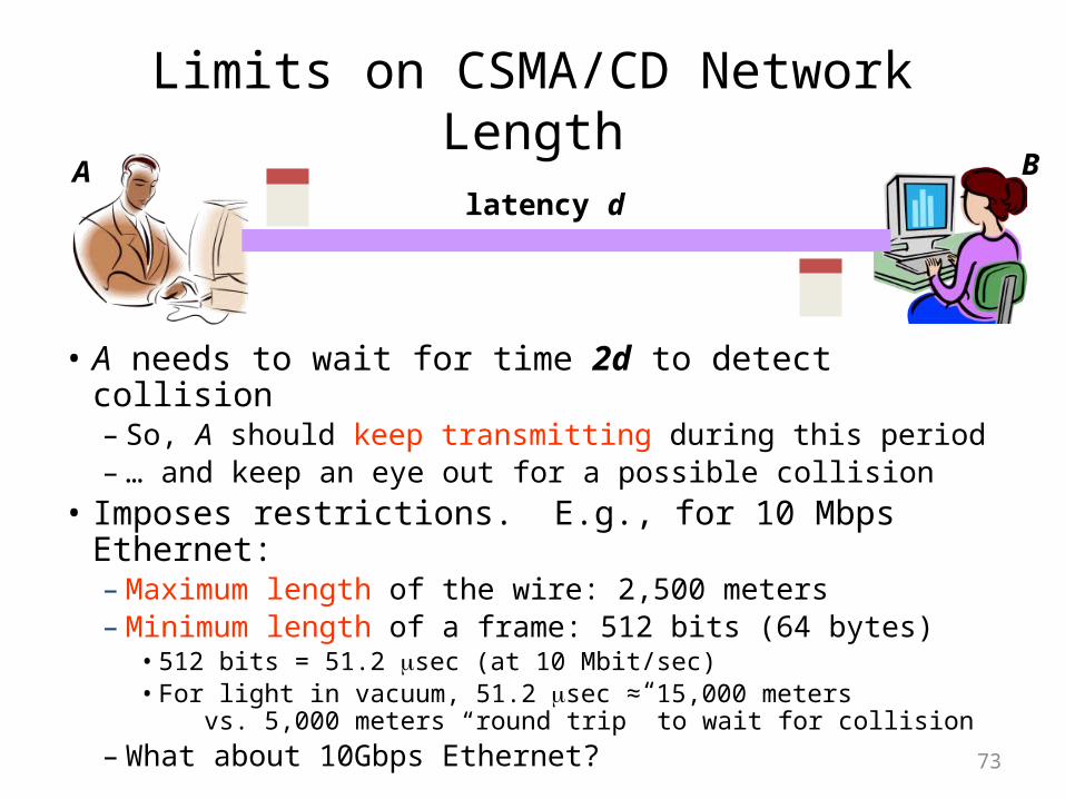
Limits on CSMA/CD Network Length

• A needs to wait for time 2d to detect collision– So, A should keep transmitting during this period– … and keep an eye out for a possible collision

• Imposes restrictions. E.g., for 10 Mbps Ethernet:– Maximum length of the wire: 2,500 meters– Minimum length of a frame: 512 bits (64 bytes)

• 512 bits = 51.2 sec (at 10 Mbit/sec)• For light in vacuum, 51.2 sec ≈ 15,000 meters

vs. 5,000 meters “round trip” to wait for collision– What about 10Gbps Ethernet?

latency dA B

74

Performance of CSMA/CD• Time wasted in collisions

– Proportional to distance d• Time spend transmitting a packet

– Packet length p divided by bandwidth b• Rough estimate for efficiency (K some constant)

• Note:– For large packets, small distances, E ~ 1– As bandwidth increases, E decreases– That is why high-speed LANs are all switched

75

Benefits of Ethernet

• Easy to administer and maintain• Inexpensive• Increasingly higher speed• Evolvable!

Evolution of Ethernet

• Changed everything except the frame format– From single coaxial cable to hub-based star– From shared media to switches– From electrical signaling to optical

• Lesson #1– The right interface can accommodate many changes – Implementation is hidden behind interface

• Lesson #2– Really hard to displace the dominant technology– Slight performance improvements are not enough

76

77

Ethernet: CSMA/CD Protocol

• Carrier sense: wait for link to be idle• Collision detection: listen while transmitting

– No collision: transmission is complete– Collision: abort transmission & send jam signal

• Random access: binary exponential back-off– After collision, wait a random time before trying again– After mth collision, choose K randomly from {0, …, 2m-1}– … and wait for K*512 bit times before trying again

• Using min packet size as “slot”• If transmission occurring when ready to send, wait until end of

transmission (CSMA)

Binary Exponential Backoff (BEB)

• Think of time as divided in slots• After each collision, pick a slot randomly within next 2m

slots– Where m is the number of collisions since last successful

transmission

• Questions:– Why backoff? – Why random? – Why 2m?– Why not listen while waiting?

78

Behavior of BEB Under Light Load

Look at collisions between two nodes• First collision: pick one of the next two slots

– Chance of success after first collision: 50%– Average delay 1.5 slots

• Second collision: pick one of the next four slots– Chance of success after second collision: 75%– Average delay 2.5 slots

• In general: after mth collision– Chance of success: 1-2-m

– Average delay (in slots): ½ + 2(m-1)

79

BEB: Theory vs Reality

In theory, there is no difference between theory and practice. But, in practice, there is.

80

BEB Reality

• Performs well (far from optimal, but no one cares)– Large packets are ~23 times as large as minimal

slot

• Is now mostly irrelevant– Almost all current ethernets are switched

81

BEB Theory

• A very interesting algorithm

• Stability for finite N only proved in 1985– Ethernet can handle nonzero traffic load without collapse

• All backoff algorithms unstable for infinite N (1985)– Poisson model: infinite user pool, total demand is finite

• Not of practical interest, but gives important insight– Multiple access should be in your “bag of tricks”

82

Question

• Two hosts, each with infinite packets to send

• What happens under BEB?

• Throughput high or low?

• Bandwidth shared equally or not?

83

MAC “Channel Capture” in BEB

• Finite chance that first one to have a successful transmission will never relinquish the channel– The other host will never send a packet

• Therefore, asymptotically channel is fully utilized and completely allocated to one host

84

Example

• Two hosts, each with infinite packets to send– Slot 1: collision– Slot 2: each resends with prob ½

• Assume host A sends, host B does not

– Slot 3: A and B both send (collision)– Slot 4: A sends with probability ½, B with prob. ¼

• Assume A sends, B does not

– Slot 5: A definitely sends, B sends with prob. ¼• Assume collision

– Slot 6: A sends with probability ½, B with prob. 1/8

• Conclusion: if A gets through first, the prob. of B sending successfully halves with each collision

85

Another Question

• Hosts now have large but finite # packets to send

• What happens under BEB?

• Throughput high or low?

86

Answer

• Efficiency less than one, no matter how many packets

• Time you wait for loser to start is proportion to time winner was sending….

87

Different Backoff Functions

• Exponential: backoff ~ ai

– Channel capture?– Efficiency?

• Superlinear polynomial: backoff ~ ip p>1– Channel capture?– Efficiency?

• Sublinear polynomial: backoff ~ ip p≤1– Channel capture?– Efficiency?

88

Different Backoff Functions

• Exponential: backoff ~ ai

– Channel capture (loser might not send until winner idle)

– Efficiency less than 1 (time wasted waiting for loser to start)

• Superlinear polynomial: backoff ~ ip p>1– Channel capture– Efficiency is 1 (for any finite # of hosts N)

• Sublinear polynomial: backoff ~ ip p≤1– No channel capture (loser not shut out)

– Efficiency is less than 1 (and goes to zero for large N)• Time wasted resolving collisions

89

90

Summary of MAC protocols

• channel partitioning, by time, frequency or code– Time Division, Frequency Division

• random access (dynamic), – ALOHA, S-ALOHA, CSMA, CSMA/CD– carrier sensing: easy in some technologies (wire), hard in others

(wireless)– CSMA/CD used in Ethernet– CSMA/CA used in 802.11

• taking turns– polling from central site, token passing– Bluetooth, FDDI, IBM Token Ring

91

MAC Addresses (and ARP)or How do I glue my network to my data-link?

• 32-bit IP address: – network-layer address– used to get datagram to destination IP subnet

• MAC (or LAN or physical or Ethernet) address: – function: get frame from one interface to another

physically-connected interface (same network)– 48 bit MAC address (for most LANs)

• burned in NIC ROM, also sometimes software settable

92

LAN Address (more)

• MAC address allocation administered by IEEE• manufacturer buys portion of MAC address space (to assure

uniqueness)• analogy: (a) MAC address: like Social Security Number (b) IP address: like postal address• MAC flat address ➜ portability

– can move LAN card from one LAN to another

• IP hierarchical address NOT portable– address depends on IP subnet to which node is attached

93

LAN Addresses and ARPEach adapter on LAN has unique LAN address

EthernetBroadcast address =FF-FF-FF-FF-FF-FF

= adapter

1A-2F-BB-709-AD

58-23-D7-FA-20-B0

0C-C4-11-6F-E3-98

71-6F7-2B-08-53

LAN(wired orwireless)

94

Address Resolution Protocol• Every node maintains an ARP table

– <IP address, MAC address> pair

• Consult the table when sending a packet– Map destination IP address to destination MAC address– Encapsulate and transmit the data packet

• But: what if IP address not in the table?– Sender broadcasts: “Who has IP address 1.2.3.156?”– Receiver responds: “MAC address 58-23-D7-FA-20-B0”– Sender caches result in its ARP table

95

Example: A Sending a Packet to BHow does host A send an IP packet to host B?

A

RB

96

Example: A Sending a Packet to BHow does host A send an IP packet to host B?

A

RB

1. A sends packet to R.2. R sends packet to B.

97

Host A Decides to Send Through R

A

RB

• Host A constructs an IP packet to send to B– Source 111.111.111.111, destination 222.222.222.222

• Host A has a gateway router R– Used to reach destinations outside of 111.111.111.0/24– Address 111.111.111.110 for R learned via DHCP/config

98

Host A Sends Packet Through R• Host A learns the MAC address of R’s interface

– ARP request: broadcast request for 111.111.111.110– ARP response: R responds with EE9-00-17-BB-4B

• Host A encapsulates the packet and sends to R

A

RB

99

R Decides how to Forward Packet• Router R’s adaptor receives the packet

– R extracts the IP packet from the Ethernet frame– R sees the IP packet is destined to 222.222.222.222

• Router R consults its forwarding table– Packet matches 222.222.222.0/24 via other adaptor

A

RB

100

R Sends Packet to B• Router R’s learns the MAC address of host B

– ARP request: broadcast request for 222.222.222.222– ARP response: B responds with 49-BD-D2-C7-52A

• Router R encapsulates the packet and sends to B

A

RB

101

Security Analysis of ARP• Impersonation

– Any node that hears request can answer …– … and can say whatever they want

• Actual legit receiver never sees a problem– Because even though later packets carry its IP

address, its NIC doesn’t capture them since not its MAC address

102

Key Ideas in Both ARP and DHCP

• Broadcasting: Can use broadcast to make contact– Scalable because of limited size

• Caching: remember the past for a while– Store the information you learn to reduce overhead– Remember your own address & other host’s addresses

• Soft state: eventually forget the past– Associate a time-to-live field with the information– … and either refresh or discard the information– Key for robustness in the face of unpredictable change

Why Not Use DNS-Like Tables?

• When host arrives:– Assign it an IP address that will last as long it is present– Add an entry into a table in DNS-server that maps MAC

to IP addresses

• Answer: – Names: explicit creation, and are plentiful– Hosts: come and go without informing network

• Must do mapping on demand

– Addresses: not plentiful, need to reuse and remap• Soft-state enables dynamic reuse

103

104

Hubs… physical-layer (“dumb”) repeaters:

– bits coming in one link go out all other links at same rate– all nodes connected to hub can collide with one another– no frame buffering– no CSMA/CD at hub: host NICs detect collisions

Co-ax or twisted pair

hub

105

CSMA/CD Lives….

Home Plug and similar Powerline Networking….

106

Switch(like a Hub but smarter)

• link-layer device: smarter than hubs, take active role– store, forward Ethernet frames– examine incoming frame’s MAC address, selectively forward

frame to one-or-more outgoing links when frame is to be forwarded on segment, uses CSMA/CD to access segment

• transparent– hosts are unaware of presence of switches

• plug-and-play, self-learning– switches do not need to be configured

107

Switch: allows multiple simultaneous transmissions

• hosts have dedicated, direct connection to switch

• switches buffer packets• Ethernet protocol used on each

incoming link, but no collisions; full duplex– each link is its own collision

domain• switching: A-to-A’ and B-to-B’

simultaneously, without collisions – not possible with dumb hub

A

A’

B

B’

C

C’

switch with six interfaces(1,2,3,4,5,6)

1 23

45

6

108

Switch Table

• Q: how does switch know that A’ reachable via interface 4, B’ reachable via interface 5?

• A: each switch has a switch table, each entry:– (MAC address of host, interface to

reach host, time stamp)

• looks like a routing table!• Q: how are entries created,

maintained in switch table? – something like a routing protocol?

A

A’

B

B’

C

C’

switch with six interfaces(1,2,3,4,5,6)

1 23

45

6

109

Switch: self-learning (recap)• switch learns which hosts can

be reached through which interfaces– when frame received, switch

“learns” location of sender: incoming LAN segment

– records sender/location pair in switch table

A

A’

B

B’

C

C’

1 23

45

6

A A’

Source: ADest: A’

MAC addr interface TTL

Switch table (initially empty)

A 1 60

110

Switch: frame filtering/forwarding

When frame received:

1. record link associated with sending host2. index switch table using MAC dest address3. if entry found for destination

then { if dest on segment from which frame arrived

then drop the frame else forward the frame on interface indicated } else flood

forward on all but the interface on which the frame arrived

111

Self-learning, forwarding: example A

A’

B

B’

C

C’

1 23

45

6

A A’

Source: ADest: A’

MAC addr interface TTL

Switch table (initially empty)

A 1 60

A A’A A’A A’A A’A A’

• frame destination unknown: flood

A’ A

destination A location known:

A’ 4 60

selective send

112

Interconnecting switches

• switches can be connected together

A

B

Q: sending from A to G - how does S1 know to forward frame destined to F via S4 and S3?

A: self learning! (works exactly the same as in single-switch case – flood/forward/drop)

S1

C D

E

FS2

S4

S3

H

I

G

113

Flooding Can Lead to Loops• Flooding can lead to forwarding loops

– E.g., if the network contains a cycle of switches– “Broadcast storm”

114

Solution: Spanning Trees• Ensure the forwarding topology has no loops

– Avoid using some of the links when flooding– … to prevent loop from forming

• Spanning tree – Sub-graph that covers all vertices but contains no

cycles– Links not in the spanning tree do not forward frames

Graph Has Cycles!

Graph Has No Cycles!

What Do We Know?

• Shortest paths to (or from) a node form a tree

• So, algorithm has two aspects :– Pick a root– Compute shortest paths to it

• Only keep the links on shortest-path

115

116

Constructing a Spanning Tree

• Switches need to elect a root– The switch w/ smallest identifier (MAC addr)

• Each switch determines if each interface is on the shortest path from the root– Excludes it from the tree if not

• Messages (Y, d, X)– From node X– Proposing Y as the root– And the distance is d

root

One hop

Three hops

117

Steps in Spanning Tree Algorithm

• Initially, each switch proposes itself as the root– Switch sends a message out every interface– … proposing itself as the root with distance 0– Example: switch X announces (X, 0, X)

• Switches update their view of the root– Upon receiving message (Y, d, Z) from Z, check Y’s id– If new id smaller, start viewing that switch as root

• Switches compute their distance from the root– Add 1 to the distance received from a neighbor– Identify interfaces not on shortest path to the root– … and exclude them from the spanning tree

• If root or shortest distance to it changed, “flood” updated message (Y, d+1, X)

118

Example From Switch #4’s Viewpoint

• Switch #4 thinks it is the root– Sends (4, 0, 4) message to 2 and

7

• Then, switch #4 hears from #2– Receives (2, 0, 2) message from 2– … and thinks that #2 is the root– And realizes it is just one hop

away

• Then, switch #4 hears from #7– Receives (2, 1, 7) from 7– And realizes this is a longer path– So, prefers its own one-hop path– And removes 4-7 link from the tree

1

2

3

4

5

67

119

Example From Switch #4’s Viewpoint

• Switch #2 hears about switch #1– Switch 2 hears (1, 1, 3) from 3– Switch 2 starts treating 1 as root– And sends (1, 2, 2) to neighbors

• Switch #4 hears from switch #2– Switch 4 starts treating 1 as root– And sends (1, 3, 4) to neighbors

• Switch #4 hears from switch #7– Switch 4 receives (1, 3, 7) from 7– And realizes this is a longer path– So, prefers its own three-hop path– And removes 4-7 Iink from the

tree

1

2

3

4

5

67

120

Robust Spanning Tree Algorithm

• Algorithm must react to failures– Failure of the root node

• Need to elect a new root, with the next lowest identifier

– Failure of other switches and links• Need to recompute the spanning tree

• Root switch continues sending messages– Periodically reannouncing itself as the root (1, 0, 1)– Other switches continue forwarding messages

• Detecting failures through timeout (soft state)– If no word from root, times out and claims to be the root– Delay in reestablishing spanning tree is major problem– Work on rapid spanning tree algorithms…

121

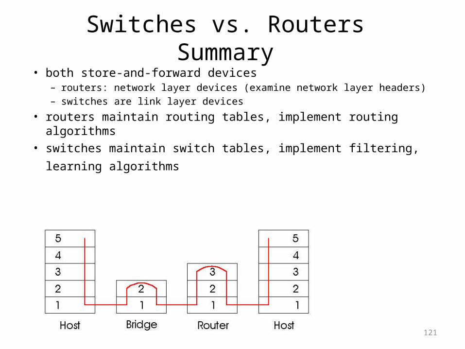
Switches vs. Routers Summary• both store-and-forward devices

– routers: network layer devices (examine network layer headers)– switches are link layer devices

• routers maintain routing tables, implement routing algorithms• switches maintain switch tables, implement filtering, learning

algorithms

122

Wireless

123

124

Metrics for evaluation / comparison of wireless technologies• Bitrate or Bandwidth• Range - PAN, LAN, MAN, WAN • Two-way / One-way • Multi-Access / Point-to-Point• Digital / Analog• Applications and industries• Frequency – Affects most physical properties:

Distance (free-space loss)Penetration, Reflection, AbsorptionEnergy proportionality Policy: Licensed / Deregulated

Line of Sight (Fresnel zone)Size of antenna

Determined by wavelength – )

125

Modern art?

126

The Wireless Spectrum

127

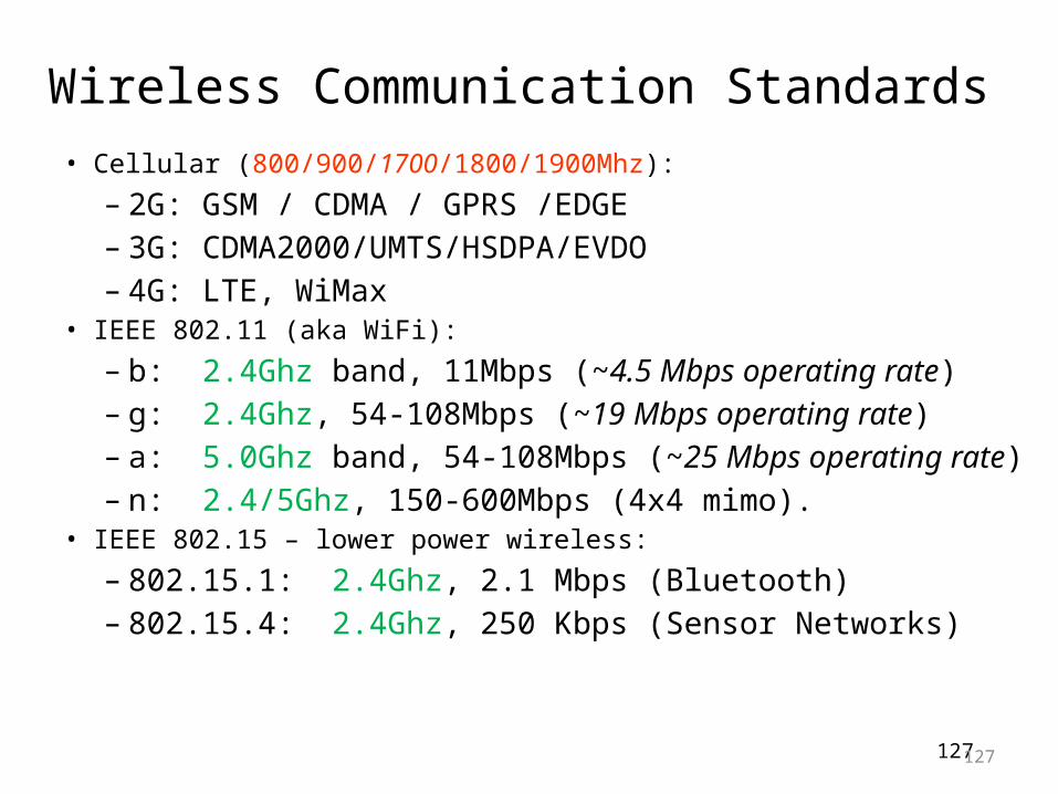
Wireless Communication Standards • Cellular (800/900/1700/1800/1900Mhz):

– 2G: GSM / CDMA / GPRS /EDGE– 3G: CDMA2000/UMTS/HSDPA/EVDO – 4G: LTE, WiMax

• IEEE 802.11 (aka WiFi):

– b: 2.4Ghz band, 11Mbps (~4.5 Mbps operating rate)– g: 2.4Ghz, 54-108Mbps (~19 Mbps operating rate)– a: 5.0Ghz band, 54-108Mbps (~25 Mbps operating rate)– n: 2.4/5Ghz, 150-600Mbps (4x4 mimo).

• IEEE 802.15 – lower power wireless:

– 802.15.1: 2.4Ghz, 2.1 Mbps (Bluetooth)– 802.15.4: 2.4Ghz, 250 Kbps (Sensor Networks)

127

128

Wireless Link Characteristics

128

(Figure Courtesy of Kurose and Ross)

Antennas / Aerials• An electrical device which converts electric

currents into radio waves, and vice versa.

129

Q: What does “higher-gain antenna” mean?A: Antennas are passive devices –

more gain means focused and more directional.Directionality means more energy gets to where it needs to go and less interference everywhere.

What are omni-directional antennas?

2-3dB 8-12dB 15-18dB 28-34dB

What has changed?

130

How many radios/antennas ?• WiFi 802.11n (maybe MiMo?)• 2G - GSM• 3G – HSDPA+• 4G – LTE• Bluetooth (4.0)• NFC• GPS Receiver• FM-Radio receiver

(antenna is the headphones cable)

131

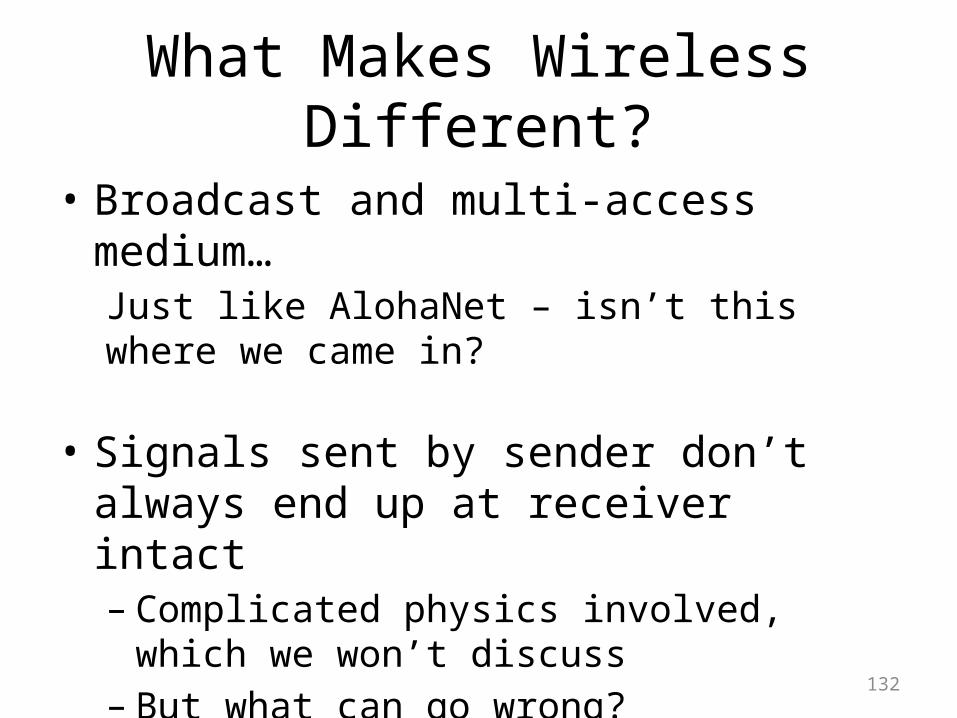
What Makes Wireless Different?

• Broadcast and multi-access medium…Just like AlohaNet – isn’t this where we came in?

• Signals sent by sender don’t always end up at receiver intact– Complicated physics involved, which we won’t

discuss– But what can go wrong?

132

Path Loss / Path Attenuation

• Free Space Path Loss:d = distanceλ = wave lengthf = frequencyc = speed of light

• Reflection, Diffraction, Absorption• Terrain contours (Urban, Rural, Vegetation).• Humidity

133

134

Multipath Effects

• Signals bounce off surface and interfere with one another

• Self-interference

134

S R

Ceiling

Floor

135

Ideal Radios(courtesy of Gilman Tolle and Jonathan Hui, ArchRock)

136

Real Radios(courtesy of Gilman Tolle and Jonathan Hui, ArchRock)

137137

The Amoeboed “cell”(courtesy of David Culler, UCB)

Signal

Noise

Distance

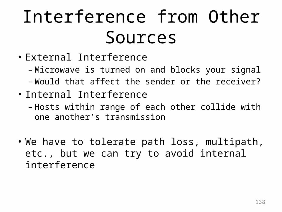
Interference from Other Sources

• External Interference– Microwave is turned on and blocks your signal– Would that affect the sender or the receiver?

• Internal Interference– Hosts within range of each other collide with one

another’s transmission

• We have to tolerate path loss, multipath, etc., but we can try to avoid internal interference

138

SNR – the key to communication:

139

Bitrate (aka data-rate) The higher the SNR –

the higher the (theoretical) bitrate.

Modern radios use adaptive /dynamic bitrates.

Q: In face of loss, should we decrease or increase the bitrate?

A: If caused by free-space loss or multi-path fading -lower the bitrate. If external interference - often higher bitrates (shorter bursts) are probabilistically better.

Signal to Noise Ratio

140

Wireless Bit Errors• The lower the SNR (Signal/Noise) the higher the Bit Error

Rate (BER)• We could make the signal stronger…• Why is this not always a good idea?

– Increased signal strength requires more power– Increases the interference range of the sender, so you

interfere with more nodes around you• And then they increase their power…….

• How would TCP behave in face of losses?– TCP conflates loss (congestion) with loss local errors

• Local link-layer Error Correction schemes can correct some problems (should be TCP aware). 140

141141

802.11aka - WiFi … What makes it special?

Deregulation > Innovation > Adoption > Lower cost = Ubiquitous technology

142

802.11 Architecture

• Designed for limited area• AP’s (Access Points) set to specific channel• Broadcast beacon messages with SSID (Service Set Identifier) and MAC Address

periodically• Hosts scan all the channels to discover the AP’s

– Host associates with AP142

802.11 frames exchanges

802.3 (Ethernet) frames exchanged

Wireless Multiple Access Technique?

• Carrier Sense?– Sender can listen before sending– What does that tell the sender?

• Collision Detection?– Where do collisions occur?– How can you detect them?

143

144144

• A and C can both send to B but can’t hear each other

– A is a hidden terminal for C and vice versa• Carrier Sense will be ineffective

Hidden Terminals

A B C

transmit range

145145

Exposed Terminals

• Exposed node: B sends a packet to A; C hears this and decides not to send a packet to D (despite the fact that this will not cause interference)!

• Carrier sense would prevent a successful transmission.

A B C D

Key Points

• No concept of a global collision– Different receivers hear different signals– Different senders reach different receivers

• Collisions are at receiver, not sender– Only care if receiver can hear the sender clearly– It does not matter if sender can hear someone else– As long as that signal does not interfere with receiver

• Goal of protocol:– Detect if receiver can hear sender– Tell senders who might interfere with receiver to shut up

146

Basic Collision Avoidance

• Since can’t detect collisions, we try to avoid them• Carrier sense:

– When medium busy, choose random interval– Wait that many idle timeslots to pass before sending

• When a collision is inferred, retransmit with binary exponential backoff (like Ethernet) – Use ACK from receiver to infer “no collision”– Use exponential backoff to adapt contention window

147

148148

CSMA/CA -MA with Collision Avoidance

• Before every data transmission – Sender sends a Request to Send (RTS) frame containing the length of the

transmission– Receiver respond with a Clear to Send (CTS) frame– Sender sends data– Receiver sends an ACK; now another sender can send data

• When sender doesn’t get a CTS back, it assumes collision

sender receiverother node in sender’s range

RTS

ACK

dataCTS

149149

CSMA/CA, con’t

• If other nodes hear RTS, but not CTS: send–Presumably, destination for first sender is out of

node’s range …

senderreceiver other node in

sender’s rangeRTS

dataCTS

data

150150

CSMA/CA, con’t

• If other nodes hear RTS, but not CTS: send– Presumably, destination for first sender is out of node’s range

…– … Can cause problems when a CTS is lost

• When you hear a CTS, you keep quiet until scheduled transmission is over (hear ACK)

sender receiverother node in sender’s range

RTS

ACK

dataCTS

151151

Overcome hidden terminal problems with contention-free protocol1. B sends to C Request To Send (RTS)2. A hears RTS and defers (to allow C to answer)3. C replies to B with Clear To Send (CTS)4. D hears CTS and defers to allow the data5. B sends to C

RTS / CTS Protocols (CSMA/CA)

B C DRTS

CTSA

B sends to C

152

Preventing Collisions Altogether• Frequency Spectrum partitioned into several channels

– Nodes within interference range can use separate channels

– Now A and C can send without any interference!• Most cards have only 1 transceiver

– Not Full Duplex: Cannot send and receive at the same time

– Aggregate Network throughput doubles 152

AB

CD

153

802.11: advanced capabilities

Rate Adaptation• base station, mobile

dynamically change transmission rate (physical layer modulation technique) as mobile moves, SNR varies

QAM256 (8 Mbps)QAM16 (4 Mbps)

BPSK (1 Mbps)

10 20 30 40SNR(dB)

BE

R

10-1

10-2

10-3

10-5

10-6

10-7

10-4

operating point

1. SNR decreases, BER increase as node moves away from base station

2. When BER becomes too high, switch to lower transmission rate but with lower BER

154

802.11: advanced capabilities

Power Management node-to-AP: “I am going to sleep until next beacon

frame”AP knows not to transmit frames to this nodenode wakes up before next beacon frame

beacon frame: contains list of mobiles with AP-to-mobile frames waiting to be sentnode will stay awake if AP-to-mobile frames to be

sent; otherwise sleep again until next beacon frame