computer animation algorithms and...
TRANSCRIPT
1
Computer AnimationRick Parent
Computer AnimationAlgorithms and Techniques
Kinematic Linkages
Computer AnimationRick Parent
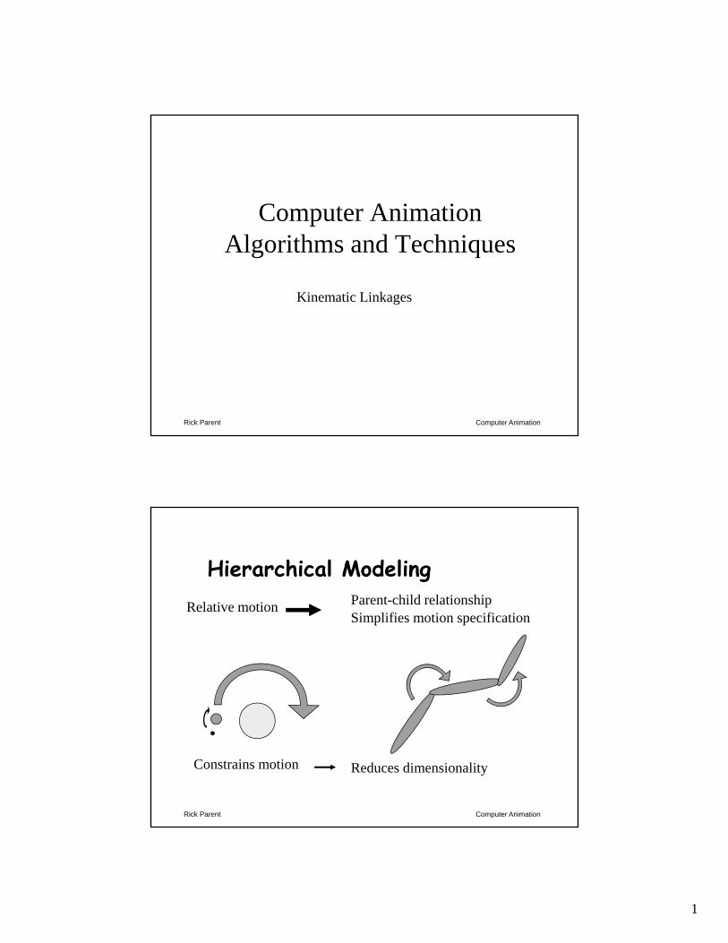
Hierarchical ModelingRelative motion Parent-child relationship
Constrains motion Reduces dimensionality
Simplifies motion specification
2
Computer AnimationRick Parent
Modeling & animating hierarchies
3 aspects1. Linkages & Joints – the relationships2. Data structure – how to represent such a hierarchy3. Converting local coordinate frames into global space
Computer AnimationRick Parent
Some termsJoint – allowed relative motion & parametersJoint Limits – limit on valid joint angle valuesLink – object involved in relative motionLinkage – entire joint-link hierarchyArmature – same as linkageEnd effector – most distant link in linkageArticulation variable – parameter of motion associated with jointPose – configuration of linkage using given set of joint anglesPose vector – complete set of joint angles for linkage
Arc – of a tree data structure – corresponds to a jointNode – of a tree data structure – corresponds to a link
3
Computer AnimationRick Parent
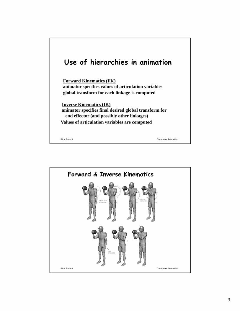
Use of hierarchies in animation
Forward Kinematics (FK)animator specifies values of articulation variables
Inverse Kinematics (IK)animator specifies final desired global transform for
end effector (and possibly other linkages)
global transform for each linkage is computed
Values of articulation variables are computed
Computer AnimationRick Parent
Forward & Inverse Kinematics
4
Computer AnimationRick Parent
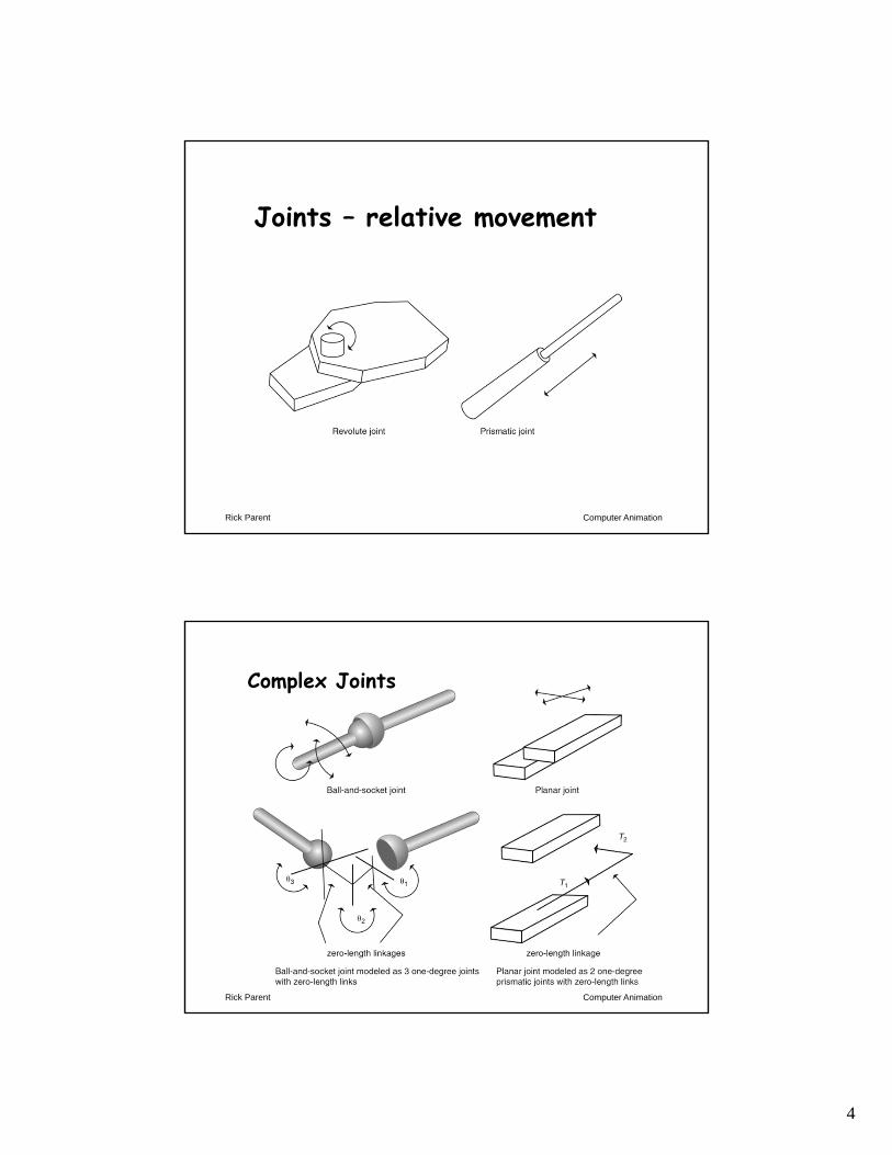
Joints – relative movement
Computer AnimationRick Parent
Complex Joints
5
Computer AnimationRick Parent
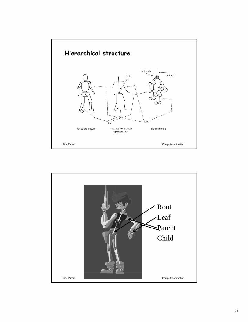
Hierarchical structure
Computer AnimationRick Parent
RootLeafParentChild

6
Computer AnimationRick Parent
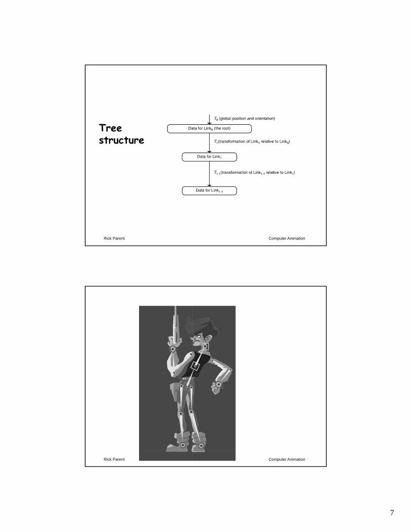
Tree structure
Computer AnimationRick Parent
Tree structure
7
Computer AnimationRick Parent
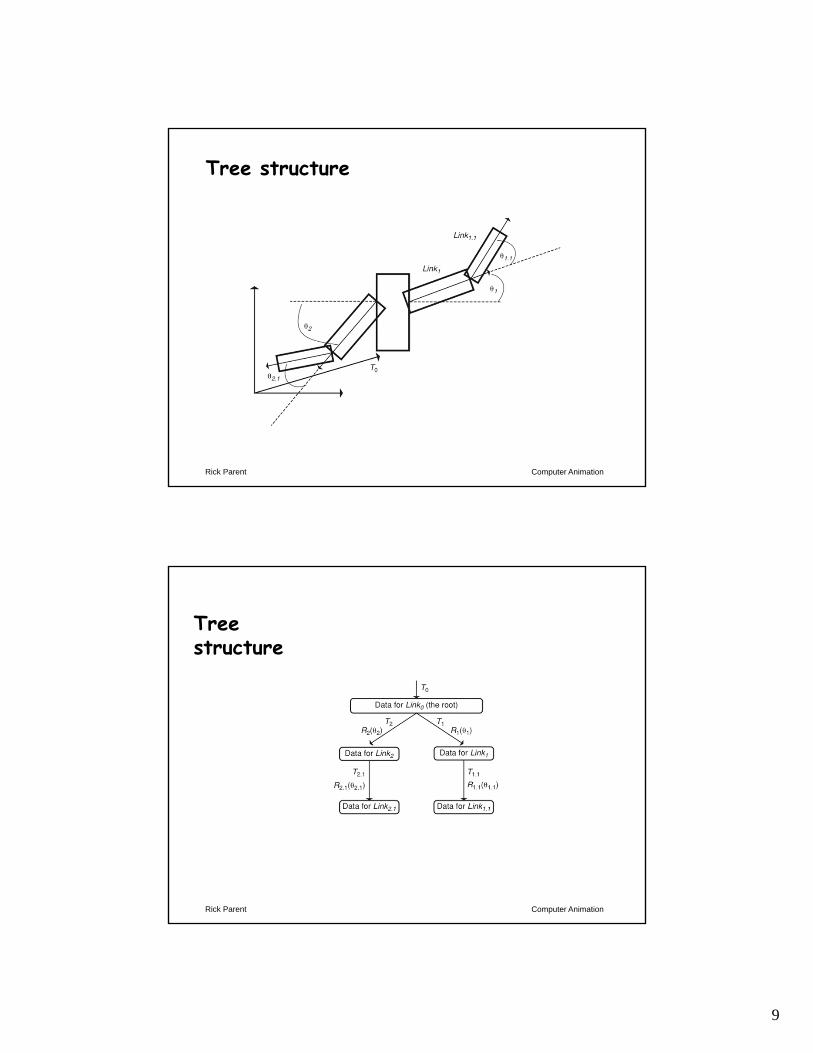
Tree structure
Computer AnimationRick Parent
8
Computer AnimationRick Parent
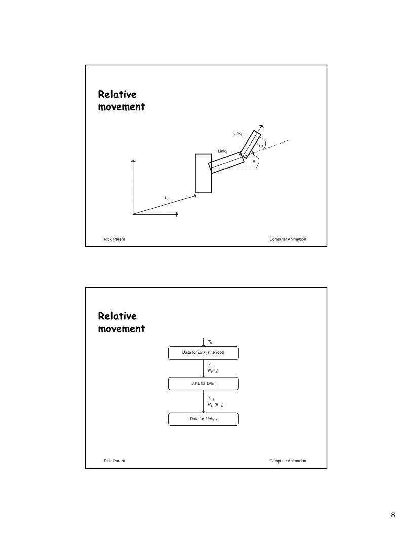
Relative movement
Computer AnimationRick Parent
Relative movement
9
Computer AnimationRick Parent
Tree structure
Computer AnimationRick Parent
Treestructure
10
Computer AnimationRick Parent
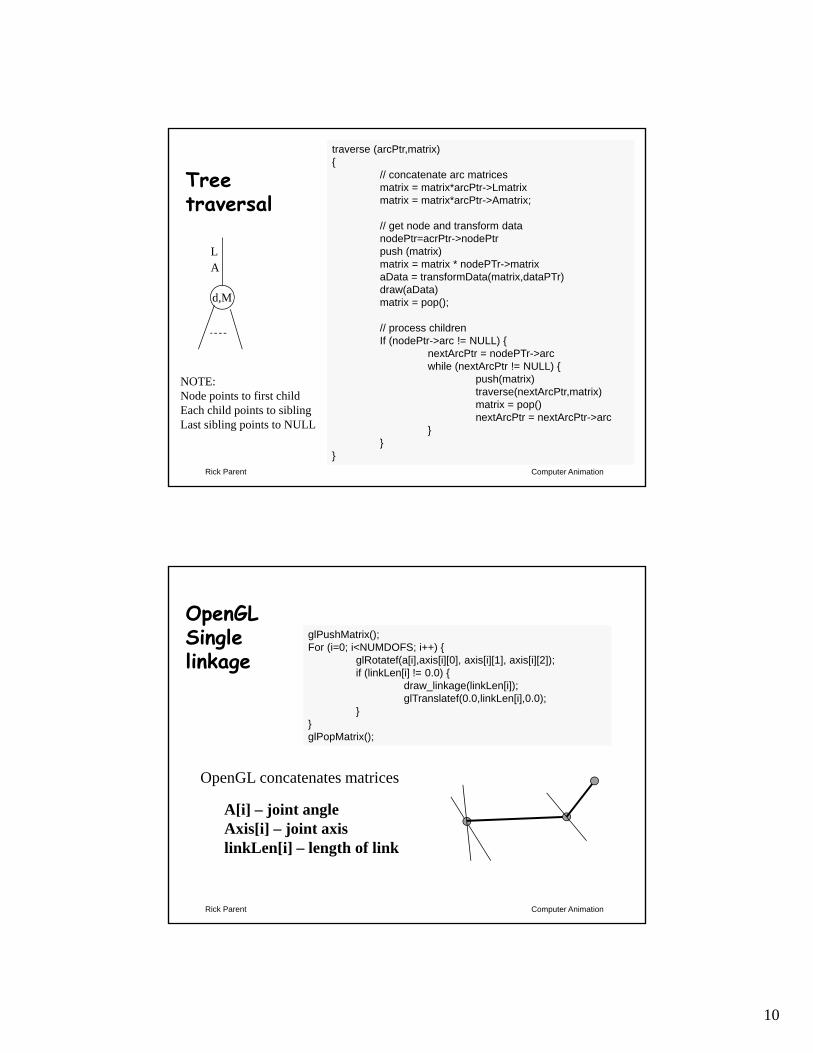
Tree traversal
traverse (arcPtr,matrix){
// concatenate arc matricesmatrix = matrix*arcPtr->Lmatrixmatrix = matrix*arcPtr->Amatrix;
// get node and transform datanodePtr=acrPtr->nodePtrpush (matrix)matrix = matrix * nodePTr->matrixaData = transformData(matrix,dataPTr)draw(aData)matrix = pop();
// process childrenIf (nodePtr->arc != NULL) {
nextArcPtr = nodePTr->arcwhile (nextArcPtr != NULL) {
push(matrix)traverse(nextArcPtr,matrix)matrix = pop()nextArcPtr = nextArcPtr->arc
}}
}
L A
d,M
NOTE: Node points to first childEach child points to siblingLast sibling points to NULL
Computer AnimationRick Parent
OpenGLSingle linkage
glPushMatrix();For (i=0; i<NUMDOFS; i++) {
glRotatef(a[i],axis[i][0], axis[i][1], axis[i][2]);if (linkLen[i] != 0.0) {
draw_linkage(linkLen[i]);glTranslatef(0.0,linkLen[i],0.0);
}}glPopMatrix();
A[i] – joint angleAxis[i] – joint axislinkLen[i] – length of link
OpenGL concatenates matrices
11
Computer AnimationRick Parent
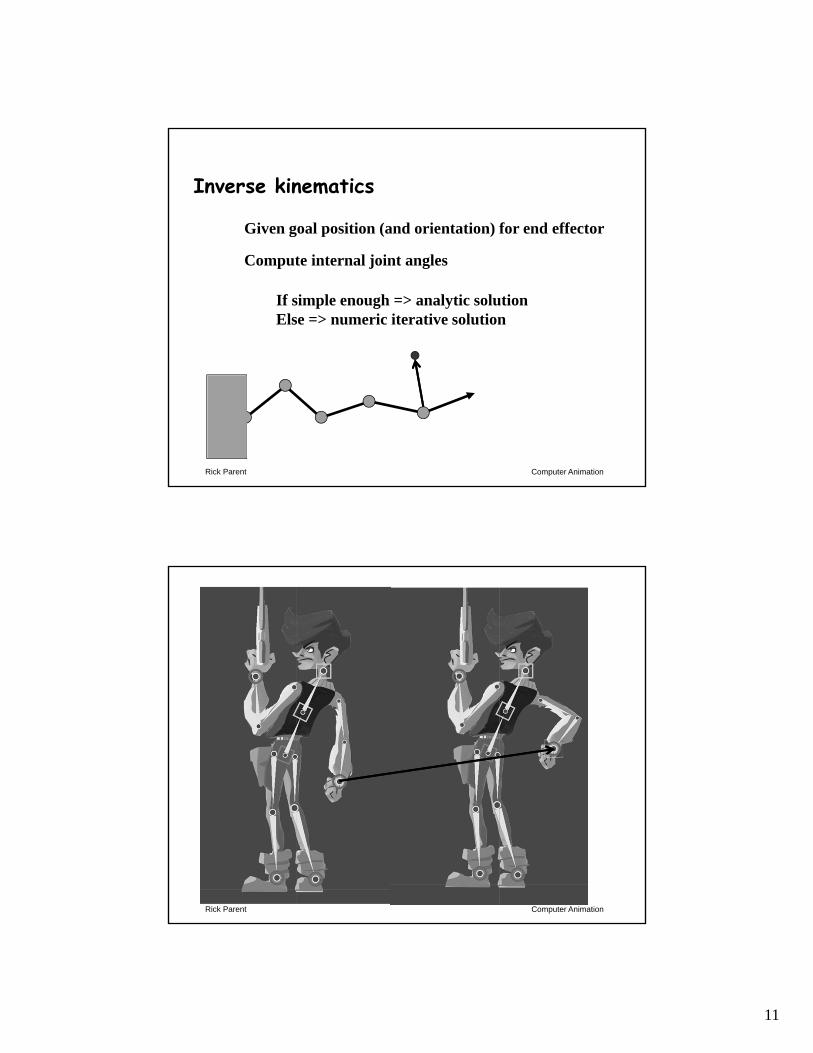
Inverse kinematics
Given goal position (and orientation) for end effector
Compute internal joint angles
If simple enough => analytic solutionElse => numeric iterative solution
Computer AnimationRick Parent
12
Computer AnimationRick Parent
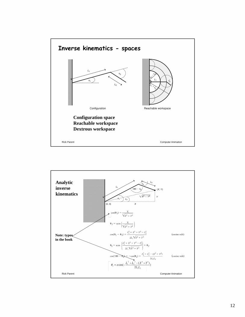
Inverse kinematics - spaces
Configuration spaceReachable workspaceDextrous workspace
Computer AnimationRick Parent
Analyticinverse kinematics
Note: typos in the book

13
Computer AnimationRick Parent
•XY
(x,y)L1L2
(0,0)
•
•
Computer AnimationRick Parent
X=4, y=1
Sqrt(16+1) = sqrt(17) = 4.12, 13.8 = acos(4/4.12)
L1 = 3L2 = 2Theta1 = 9+16+1-4= 22/(6*4.12)=22/24.7, acos(.89) = 27.1+ 34.5 = 61.6
•
14
Computer AnimationRick Parent
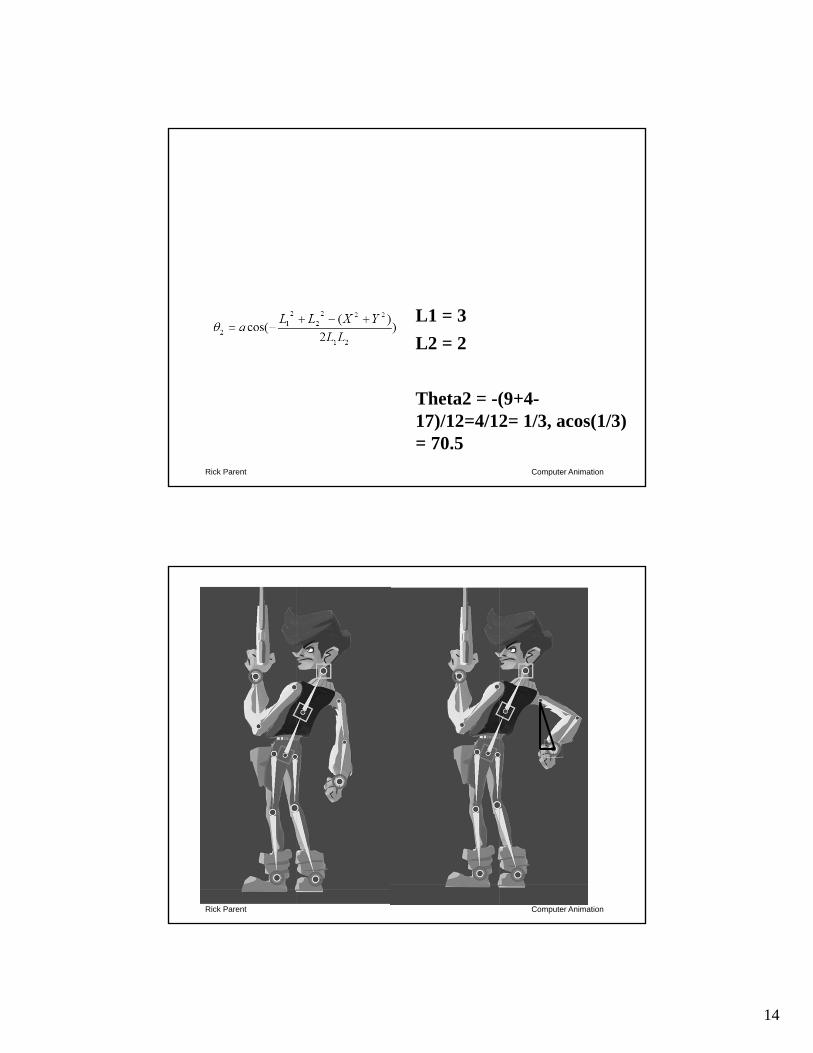
L1 = 3L2 = 2
Theta2 = -(9+4-17)/12=4/12= 1/3, acos(1/3) = 70.5
Computer AnimationRick Parent
15
Computer AnimationRick Parent
Computer AnimationRick Parent
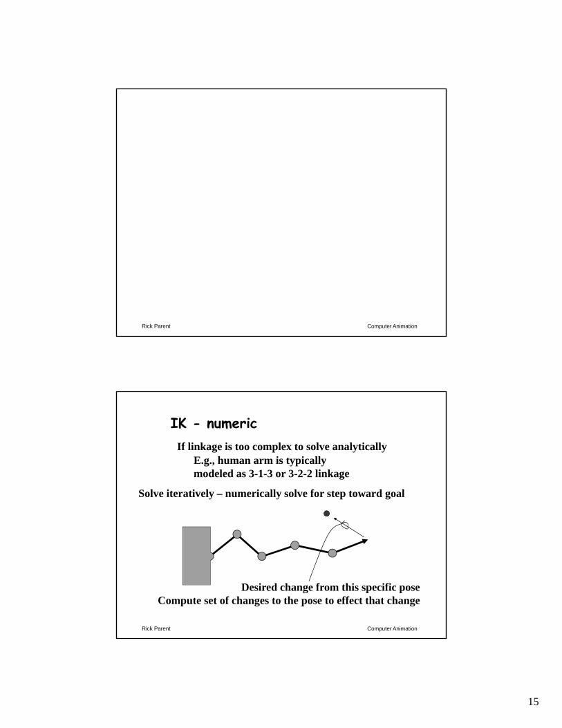
IK - numericIf linkage is too complex to solve analytically
Desired change from this specific poseCompute set of changes to the pose to effect that change
Solve iteratively – numerically solve for step toward goal
E.g., human arm is typically modeled as 3-1-3 or 3-2-2 linkage
16
Computer AnimationRick Parent
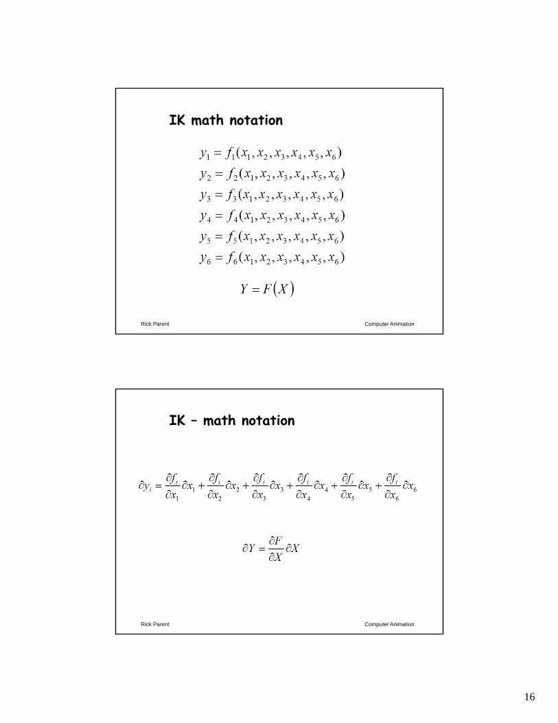
IK math notation
Computer AnimationRick Parent
IK – math notation
17
Computer AnimationRick Parent
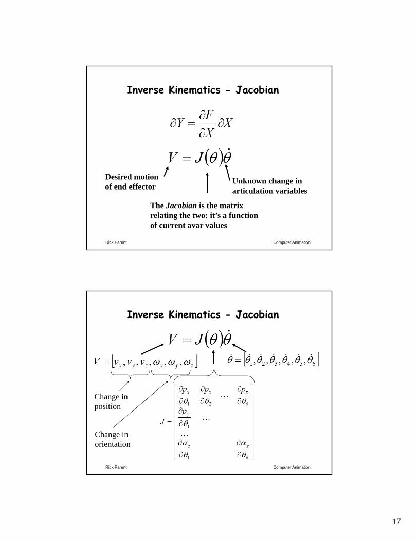
Inverse Kinematics - Jacobian
Desired motion of end effector
Unknown change in articulation variables
The Jacobian is the matrix relating the two: it’s a function of current avar values
Computer AnimationRick Parent
Inverse Kinematics - Jacobian
Change in position
Change in orientation
18
Computer AnimationRick Parent
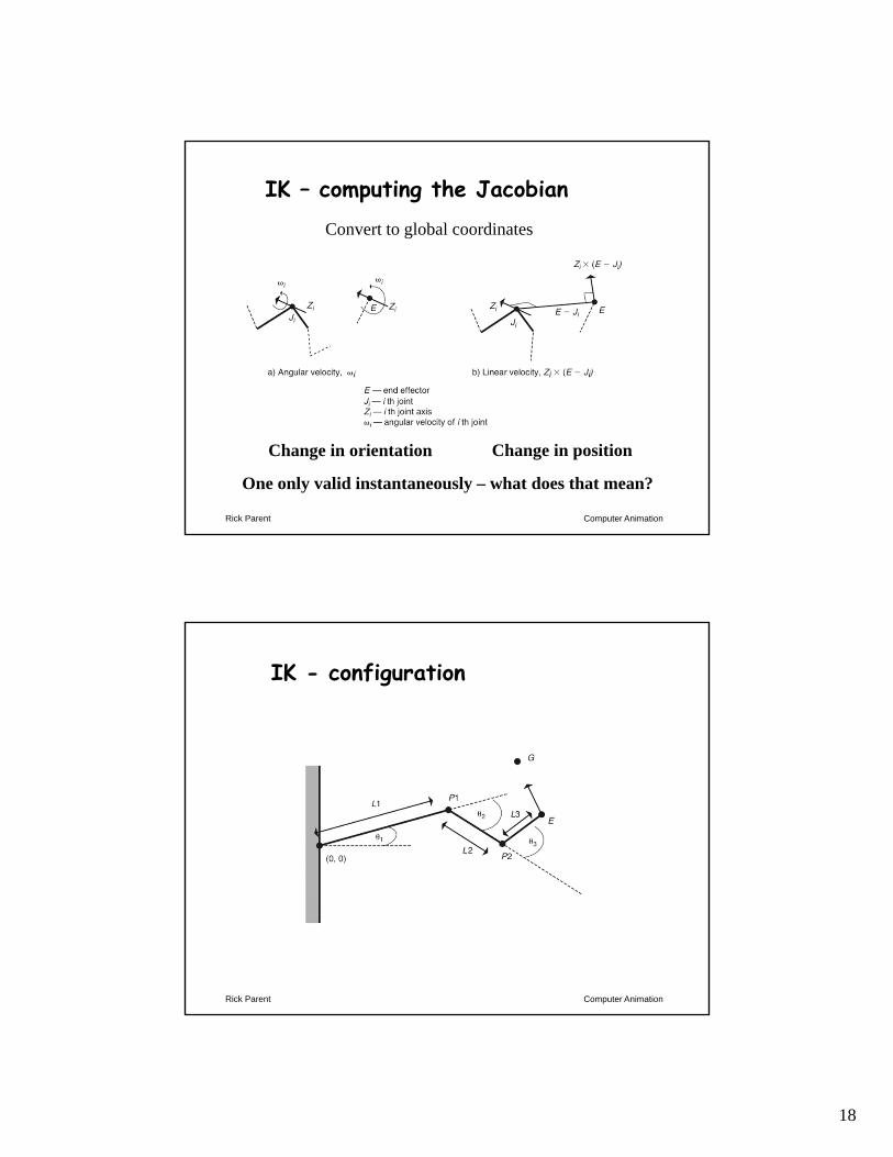
IK – computing the Jacobian
One only valid instantaneously – what does that mean?
Convert to global coordinates
Change in positionChange in orientation
Computer AnimationRick Parent
IK - configuration
19
Computer AnimationRick Parent
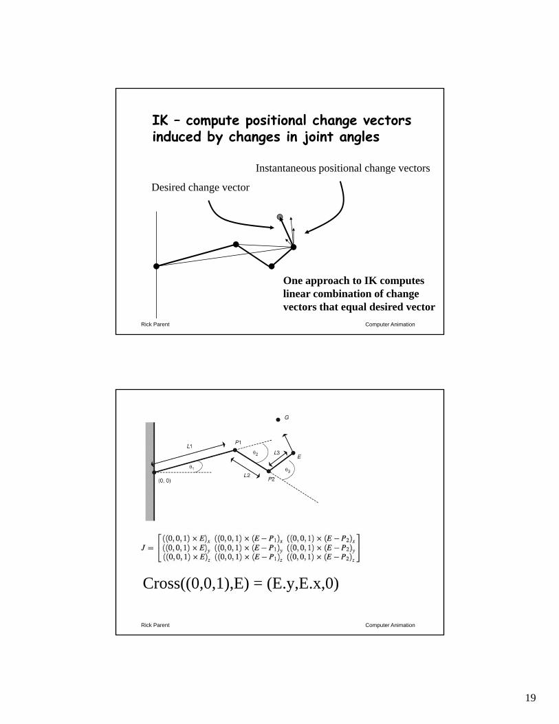
IK – compute positional change vectors induced by changes in joint angles
Instantaneous positional change vectors
Desired change vector
One approach to IK computes linear combination of change vectors that equal desired vector
Computer AnimationRick Parent
Cross((0,0,1),E) = (E.y,E.x,0)
20
Computer AnimationRick Parent
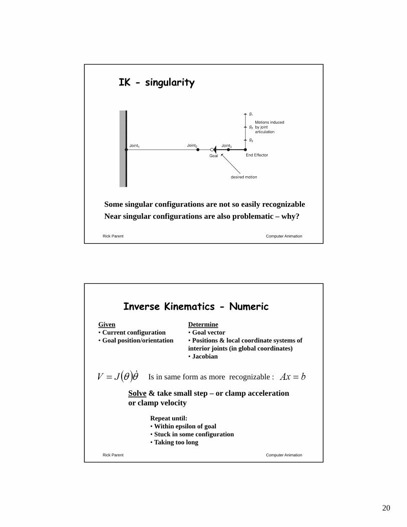
IK - singularity
Some singular configurations are not so easily recognizableNear singular configurations are also problematic – why?
Computer AnimationRick Parent
Inverse Kinematics - NumericGiven• Current configuration• Goal position/orientation
Determine• Goal vector• Positions & local coordinate systems of interior joints (in global coordinates)• Jacobian
Solve & take small step – or clamp acceleration or clamp velocity
Repeat until:• Within epsilon of goal• Stuck in some configuration• Taking too long
Is in same form as more recognizable :
21
Computer AnimationRick Parent
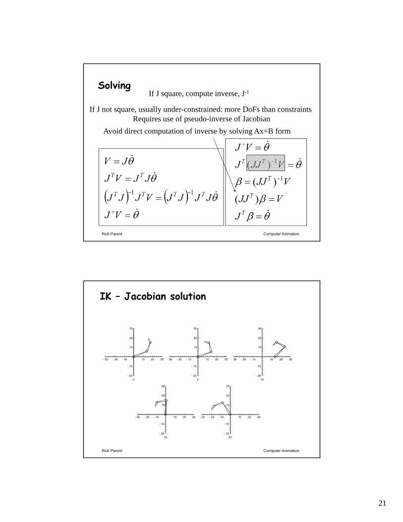
Solving
If J not square, usually under-constrained: more DoFs than constraints Requires use of pseudo-inverse of Jacobian
If J square, compute inverse, J-1
Avoid direct computation of inverse by solving Ax=B form
Computer AnimationRick Parent
IK – Jacobian solution
22
Computer AnimationRick Parent
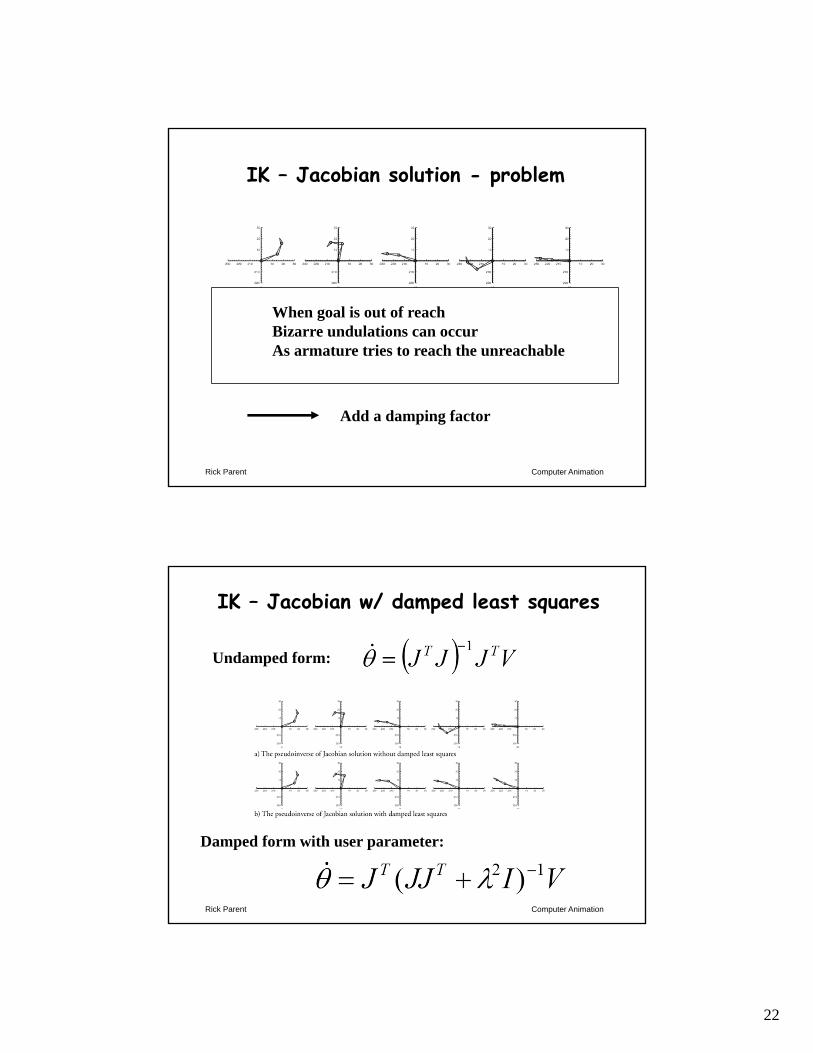
IK – Jacobian solution - problem
When goal is out of reachBizarre undulations can occurAs armature tries to reach the unreachable
Add a damping factor
Computer AnimationRick Parent
IK – Jacobian w/ damped least squares
Undamped form:
Damped form with user parameter:
23
Computer AnimationRick Parent
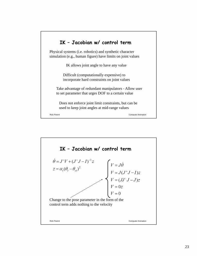
IK – Jacobian w/ control term
Take advantage of redundant manipulators - Allow user to set parameter that urges DOF to a certain value
Does not enforce joint limit constraints, but can be used to keep joint angles at mid-range values
Physical systems (i.e. robotics) and synthetic character simulation (e.g., human figure) have limits on joint values
IK allows joint angle to have any value
Difficult (computationally expensive) to incorporate hard constraints on joint values
Computer AnimationRick Parent
IK – Jacobian w/ control term
Change to the pose parameter in the form of the control term adds nothing to the velocity
24
Computer AnimationRick Parent
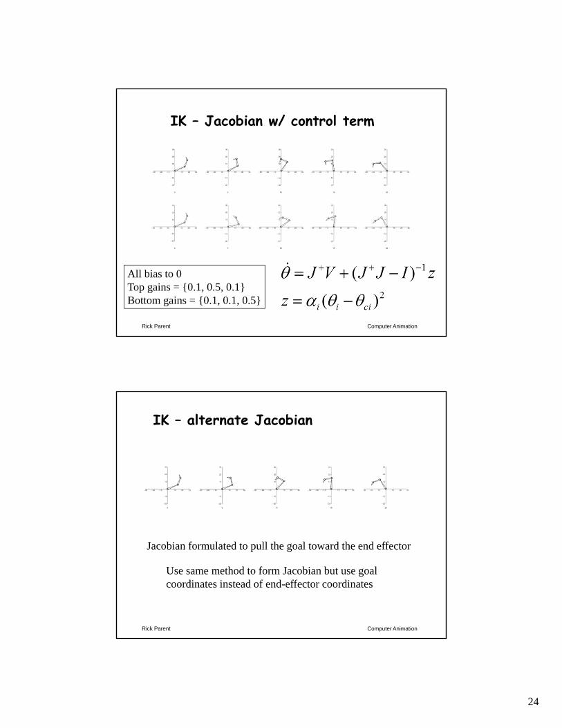
IK – Jacobian w/ control term
All bias to 0Top gains = {0.1, 0.5, 0.1}Bottom gains = {0.1, 0.1, 0.5}
Computer AnimationRick Parent
IK – alternate Jacobian
Jacobian formulated to pull the goal toward the end effector
Use same method to form Jacobian but use goal coordinates instead of end-effector coordinates
25
Computer AnimationRick Parent
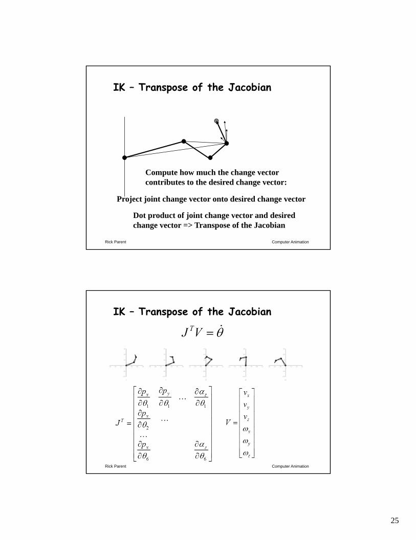
IK – Transpose of the Jacobian
Compute how much the change vector contributes to the desired change vector:
Project joint change vector onto desired change vector
Dot product of joint change vector and desired change vector => Transpose of the Jacobian
Computer AnimationRick Parent
IK – Transpose of the Jacobian

26
Computer AnimationRick Parent
IK – cyclic coordinate descent
Consider one joint at a time, from outside inAt each joint, choose update that best gets end effector to goal position
In 2D – pretty simple
EFGoal
Ji
axisi
Heuristic solution
Computer AnimationRick Parent
IK – cyclic coordinate descent
In 3D, a bit more computation is needed
27
Computer AnimationRick Parent
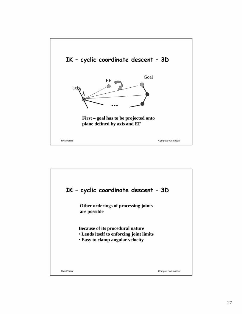
IK – cyclic coordinate descent – 3D
EFGoal
Ji
axisi
First – goal has to be projected onto plane defined by axis and EF
Computer AnimationRick Parent
IK – cyclic coordinate descent – 3D
Other orderings of processing joints are possible
Because of its procedural nature• Lends itself to enforcing joint limits• Easy to clamp angular velocity
28
Computer AnimationRick Parent
Inverse kinematics - review
Analytic methodForming the JacobianNumeric solutions
Pseudo-inverse of the JacobianJ+ with dampingJ+ with control termAlternative JacobianTranspose of the JacobianCyclic Coordinate Descent (CCD)
Computer AnimationRick Parent
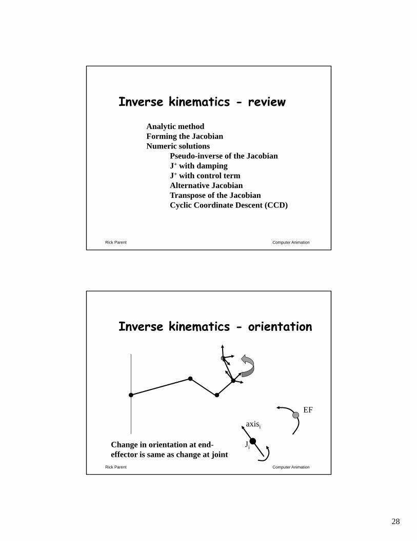
Inverse kinematics - orientation
Change in orientation at end-effector is same as change at joint
Ji
axisi
EF
29
Computer AnimationRick Parent
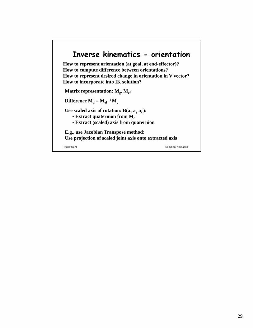
Inverse kinematics - orientationHow to represent orientation (at goal, at end-effector)?How to compute difference between orientations?How to represent desired change in orientation in V vector?How to incorporate into IK solution?
Matrix representation: Mg, Mef
Difference Md = Mef-1 Mg
Use scaled axis of rotation: B(ax ay az ):• Extract quaternion from Md• Extract (scaled) axis from quaternion
E.g., use Jacobian Transpose method: Use projection of scaled joint axis onto extracted axis