computations with oracles that measure vanishing...
TRANSCRIPT
Under consideration for publication in Math. Struct. in Comp. Science
Computations with oracles that measurevanishing quantities
Edwin Beggs1, Jose Felix Costa2, Diogo Pocas3 & John V. Tucker1
1 College of Science, Swansea University, Swansea, SA2 8PP, Wales, United Kingdom2 Instituto Superior Tecnico, Universidade de Lisboa, Portugal3 Centro de Matematica e Aplicacoes Fundamentais da Universidade de Lisboa, Portugal
Received May 23, 2015
We consider computation with real numbers that arise through a process of physical
measurement. We have developed a theory in which physical experiments that measure
quantities can be used as oracles to algorithms and we have begun to classify the
computational power of various forms of experiment using non-uniform complexity
classes. Earlier, in (Beggs, Costa & Tucker 2014), we observed that measurement can be
viewed as a process of comparing a rational number z – a test quantity – with a real
number y – an unknown quantity; each oracle call performs such a comparison.
Experiments can then be classified into three categories, that correspond with being able
to return test results
z < y or z > y or timeout,
z < y or timeout,
z 6= y or timeout.
These categories are called two-sided, threshold and vanishing experiments, respectively.
The iterative process of comparing generates a real number y. The computational power
of two-sided and threshold experiments were analysed in several papers, including
(Beggs, Costa, Loff & Tucker 2008; Beggs, Costa, Loff & Tucker 2009; Beggs, Costa,
Pocas & Tucker 2013a; Beggs, Costa & Tucker 2010b; Beggs, Costa & Tucker 2014). In
this paper we attack the subtle problem of measuring physical quantities that vanish in
some experimental conditions (e.g., Brewster’s angle in optics). We analyse in detail a
simple generic vanishing experiment for measuring mass and develop general techniques
based on parallel experiments, statistical analysis and timing notions that enable us to
prove lower and upper bounds for its computational power in different variants. We end
with a comparison of various results for all three forms of experiments and suitable
postulate for computation involving analogue inputs that breaks the Church-Turing
barrier.
1. Introduction
Computation theory is about data, algorithms, programs and machines. When the data
are real numbers, our computations operate with approximations: typically, a real number
y that is given as a sequence
Edwin Beggs, Jose Felix Costa, Diogo Pocas & John V Tucker 2
z0, z1, z2, . . . , zk, . . .
of rational numbers that are approximations to y. Indeed, the real number y is defined
as an idealisation of a process of rational approximation in the form of an equivalence
class of rational Cauchy sequences. Finite computations with the infinite representations
of y operate with the finite representations of rational numbers z0, z1, z2, . . . , zk, . . . to-
gether with a modulus of convergence.† Our computability theories are not concerned
with where the real numbers come from: the intuitions and abstractions of real number
computation form a world of their own. This is entirely satisfactory if the real number
comes from another computation. However, let us expand this world somewhat by asking
the question:
Suppose a real number y that enters a computation comes from a process of physical
measurement. How can we model this process? What effect does measurement have on
our theory of real number computation?
Whilst logical aspects of measurement have been theorised – see the magnum opus
(Krantz, Suppes, Luce & Tversky 1990) – computable aspects of measurement have been
rather neglected. An early analysis on the computability of physical constants is (Geroch
& Hartle 1986), where an informal attempt at defining measurement can be found. We
are developing a new theory that combines measurement and computation, in a series of
papers that examines a range of experiments and their effects on computation: (Beggs,
Costa, Loff & Tucker 2008; Beggs, Costa, Loff & Tucker 2009; Beggs, Costa & Tucker
2010a; Beggs, Costa & Tucker 2010c; Beggs, Costa & Tucker 2010b; Beggs, Costa &
Tucker 2012b; Beggs, Costa & Tucker 2012a; Beggs, Costa & Tucker 2014). Like Geroche
and Hartle, our study is rooted in physics but it uses a methodology that combines
physical theories with the rich concepts and results of computability and complexity
theory. An abstract study of measurement, tailored to computable analysis, is (Pauly
2005); Pauly uses the representation methods characteristic of the type 2 computability
models – e.g., after (Weihrauch 2000) – to model an interface to the data extracted from
physical behaviour.
In this paper we will be able to reach some preliminary conclusions by solving a
remaining subtle problem, that of measuring physical quantities that vanish in some
experimental conditions.
What is measurement? The essence of any measurement is a comparison: see (Hempel
1952) where comparisons are based on events in the experimental setup. Let the real
number y be the value of the unknown quantity we wish to measure. Then a comparison
is made with a known quantity z; this quantity is a rational number because it describes
the quantity using units of measurement (e.g., 3.75 means 3 whole units and 34 of a unit).
In running an experiment one expects there to be a schedule that allocates reasonable
waiting times. The actual experimental time is likely to be a function f of the difference
between our known quantity and the unknown value, f(|y−z|). This is evidenced by our
study of many experiments and it has become a fundamental assumption in the theory.
† The combination makes the approximation process computable.
Computations with oracles that measure vanishing quantities 3
In many experiments we expect one of the following values, where timeout indicates that
the experimental time has exceeded the allocated schedule:
z < y or z > y or timeout.
The process can be repeated with a new known quantity z′, which is easily determined by
the previous result. Thus, a sequence of measurements can be generated that approximate
y. We have studied many such experiments and call them two-sided experiments because
approximations can be found above or below y.
However, not all experiments are two-sided. In (Beggs, Costa, Pocas & Tucker 2013a;
Beggs, Costa, Pocas & Tucker 2013b), we studied experiments in which the unknown
quantities were thresholds. In this case, the process produces one of these test results:
z < y or timeout.
We showed how the process can be repeated with a new known quantity z′ determined
by the previous result and a sequence of approximate measurements generated – but the
case is complicated. We call these threshold experiments.
In this paper, we study a third form of experiment in which the unknown quantity
vanishes. In this case the process produces one of these test results:
z 6= y or timeout.
Thus, we know the unknown and known quantities are not equal but we do not know
which is larger. It is harder to see how to repeat the process with a new known quantity
z′, using the result, in order to generate a sequence that measures y. Here we give new
techniques based upon running parallel experiments, statistical analysis and exploiting
timing notions that enable us to generate a sequence and enable us to prove lower and
upper bounds for its computational power in different variants. This done we are able to
compare the various results for all three forms of experiment and draw some conclusions.
Our theory combines measurement and computation by integrating models of experi-
ments with models of computation for the data obtained. At the heart of our theory is
the idea that an experimenter measures a physical quantity by applying an experimental
procedure to equipment and that an experimental procedure is an algorithm of some
kind. We model this idea as follows:
The experimental procedure is modelled as a Turing machine. The equipment is mod-
elled as a physical device whose behaviour is governed by a physical theory. The equipment
is connected to the Turing machine as a physical oracle with a protocol to manage the
interface.
The Turing machine abstracts the experimental procedure, encoding the experimental
actions and data by a program; it also is able to process the data obtained by measure-
ment. Thus, this mathematical approach captures
(i) the measurement process;
(ii) the use the data from measurement in subsequent computations; and, indeed,
(iii) arbitrary sequences of interactions with equipment.
The protocols that manage the interface between algorithm and experiment are sophisti-
cated, controlling the precision and timings of queries to the oracle. The precision in the
data can be (a) infinite, (b) finite and unbounded, or (c) finite and fixed. The timings
Edwin Beggs, Jose Felix Costa, Diogo Pocas & John V Tucker 4
are limited, bounded by a function of the query. Finally, the computational power is
analysed under the complexity constraint of polynomial time and expressed in terms of
nonuniform complexity theory. Since non-uniform complexity seems to be little known,
for convenience, we give a quick summary in Section 3.
The models of a physical systems are based upon some fragment of a physical theory;
these fragments are parameters in all our applications for, in principle, changing the as-
sumptions about a physical model can change the computational properties. This method
of formalising the theory was seen as basic to any theoretical methodology seeking to
explore the relationship between physical systems and computation was described in our
(Beggs and Tucker 2006; Beggs and Tucker 2007a). Martin Zeigler used the idea with
great effect on the longstanding problem of defining a physical Church-Turing Thesis in
(Ziegler 2009).
In this paper, centre stage is taken by the new methods based on analysing experimen-
tal times. We use the measurement of the time to determine the computational power of
a Turing machine using a typical vanishing experiment as an oracle. In the first method,
we perform two experiments in parallel differing in only one parameter, and determine
which experiment finishes first. In the second method we time experiments by means of a
clock. These techniques introduce the problem of precision into our thinking about time.
We can ask: What is the smallest temporal resolution with which we can distinguish the
order of two events? What is the spacing between the ticks of the clock, i.e., the temporal
resolution which will be recorded as a different time on the clock output. The precision
ε in time is not asymptotic – as the precision in the quantity (i.e., ε → 0) – but rather
a tolerance that can be quantified as a function of the query. Thus, here we consider
two types of precision: precision in the time of oracle consultation and precision in the
concept to be measured.‡
In a Type I vanishing experiment two instances E and E′ of an experiment are run
with different values of a parameter (typically with one unknown value and one known
value set by the experimenter). In our main example, this parameter is a mass. The
result returned by the experiment is simply whether experiment E terminates before E′,
whether E′ terminates before E, or otherwise (i.e. neither terminate in the allowed time,
or they are judged to have terminated simultaneously). Time is compared rather than
quantified. The precision of the experiment determines how accurately the actual value
of the parameter used in the experiment corresponds to the data in the query sent by
the Turing machine. The fact that this is a vanishing experiment, rather than two-sided
or threshold, dictates the algorithm.
Theorem 1. The following are lower and upper bound results for Type I parallel methods
for the three kinds of precision:
1 If a set A is decided in polynomial time by a deterministic oracle Turing machine
coupled with a Type I vanishing quantity experiment of infinite or unbounded finite
‡ We have discussed the case of precision of the quantity in several of our earlier papers. Here we notethat the problem of errors in experiments that cannot be made arbitrarily small just by putting more
care and resources into the experiment is tackled by repeating experiments to obtain statistical data,
from which we obtain probabilistic complexity classes.

Computations with oracles that measure vanishing quantities 5
precisions, then A ∈ P/poly. If a set A is in P/poly, then A is decided by a deter-
ministic oracle Turing machine coupled with a Type I vanishing quantity experiment
of infinite or unbounded finite precisions.
2 If a set A is decided in polynomial time by an oracle Turing machine coupled with
a vanishing quantity experiment of fixed finite precision, then A ∈ BPP//log?. If a
set A is in BPP//log?, then A is decided in polynomial time by an oracle Turing
machine coupled with a vanishing quantity experiment of fixed finite precision.
In a Type II vanishing experiment an instance of an experiment is run with a parameter
determined by data in a query from the Turing machine, up to a certain precision. The
query is timed by the system clock, and an answer to the query is returned. The system
clock is taken to be incremented by integers, so the time returned actually states that the
experiment terminated between two ‘ticks’ of the system clock, thus introducing a time
resolution. A priori, we are not concerned with any ‘physical time’ for the experiment,
just the timing of termination measured by the system clock.
Theorem 2. The following are lower and upper bound results for Type II clock methods
for the three kinds of precision:
1 If a set A is decided in polynomial time by a deterministic oracle Turing machine
coupled with a Type II vanishing quantity experiment of infinite precision, then A ∈P/poly. If a set A is in P/log?, then A is decided by a oracle Turing machine coupled
with a vanishing quantity experiment of infinite precision.
2 If a set A is decided in polynomial time by a deterministic oracle Turing machine
coupled with a Type II vanishing quantity experiment of unbounded finite precision,
then A ∈ P/poly. If a set A is decided in polynomial time by a deterministic or-
acle Turing machine coupled with a Type II vanishing quantity experiment of un-
bounded finite precision and exponential protocol, then A ∈ BPP//log?. If a set A is
in BPP//log?, then A is decided by a oracle Turing machine coupled with a vanishing
quantity experiment of unbounded finite precision.
3 If a set A is decided by a deterministic oracle Turing machine coupled with a Type
II vanishing quantity experiment of fixed finite precision, then A ∈ BPP//log?. If
a set A is in BPP//log?, then A is decided in polynomial time by a oracle Turing
machine coupled with a vanishing quantity experiment of fixed precision.
Vanishing oracles are new and the methods for two-sided and threshold oracles do not
apply to them – this has led us to discover the use of timing, which raises subtle points
for the theory. The upper bound known so far for the two-sided oracles with non-infinite
precision is P/poly (except for particular types of two-sided oracles considered in (Beggs,
Costa, Loff & Tucker 2009) and (Beggs, Costa & Tucker 2012a) for which the upper
bounds are P/poly and BPP//log?, respectively). The upper bound known so far for
the threshold oracles with non-infinite precision is BPP//log2? (Beggs, Costa, Pocas &
Tucker 2013a).
In Section 2 we introduce two vanishing experiments: the measurement of Brewster’s
angle in optics and a special beam balance for mass designed for our theoretical analysis,
which we call the vanishing balance experiment (VBE for short). In Sections 4 and 8,
we discuss the operating protocols between Turing machines and stochastic oracles. In
Edwin Beggs, Jose Felix Costa, Diogo Pocas & John V Tucker 6
Sections 5, 6 and 7, we will introduce the VBE machines together with measurement
algorithms for the three types of precision. Finally, for each type of precision, we will
characterize the complexity classes decided by such machines in polynomial time. Lower
bounds are proved in Section 10 and upper bounds in the following Section 11.
2. Examples of vanishing quantity experiments
We now present two vanishing quantity experiments and adopt the second for our anal-
ysis. The first optical experiment shows that there are physical scenarios in which an
experiment yields z 6= y without yielding z < y or z > y. The second beam balance
experiment is artificial to some extent, but is a convenient to use in developing the the-
ory: measuring mass by means of a beam balance is the simplest form of experimental
comparison that is not trivial. Furthermore, each of our three types of experiment can
be demonstrated by an adaptation of the beam balance, showing that the beam balance
is a reassuringly primitive experiment, ideal for theory making.
Our methodology for any experiment begins with settling on a fragment of physical
theory sufficient to specify a model of the equipment and its behaviour (Beggs and Tucker
2006; Beggs and Tucker 2007a). However, in our examples there are some simple choices
for the assumptions.
2.1. The Brewster Angle Experiment
The Brewster Angle Experiment is an experiment based on the principles of classical
optics. It was first described as an example of vanishing value experiment in (?). The
book (Born & Wolf 1964) provides an useful reference for the experiment that we will
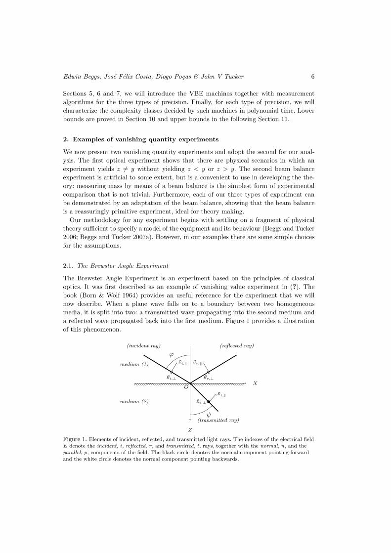
now describe. When a plane wave falls on to a boundary between two homogeneous
media, it is split into two: a transmitted wave propagating into the second medium and
a reflected wave propagated back into the first medium. Figure 1 provides a illustration
of this phenomenon.
(incident ray) (reflected ray)
(transmitted ray)
medium (1)
medium (2)
OX
Z
~Ei,⊥ ~Er,⊥
~Et,⊥
ϕ
ψ
~Ei,‖ ~Er,‖
~Et,‖
Figure 1. Elements of incident, reflected, and transmitted light rays. The indexes of the electrical fieldE denote the incident, i , reflected, r , and transmitted, t , rays, together with the normal, n, and theparallel, p, components of the field. The black circle denotes the normal component pointing forward
and the white circle denotes the normal component pointing backwards.
Computations with oracles that measure vanishing quantities 7
The experimental apparatus consists of a surface dividing two media, a projector and
a light detector. We can send a light beam into the surface with a certain incidence
angle ϕ. The electric field is perpendicular to the direction of propagation and can be
decomposed into components parallel (subscript ‖) and perpendicular (subscript ⊥) to
the plane of incidence. Let Ei,‖ and Ei,⊥ denote the components of the incident ray, Er,‖and Er,⊥ the components of the reflected ray, and Et,‖ and Et,⊥ the components of the
transmitted ray. Let ϕ be the angle of incidence and ψ be the angle of transmission.
From optics we can deduce several relations between the components of the electric field,
called Fresnel formulas:
Et,‖ =2 sinψ cosϕ
sin(ϕ+ ψ) cos(ϕ− ψ)Ei,‖, Et,⊥ =
2 sinϕ cosψ
sin(ϕ+ ψ)Ei,⊥ ,
Er,‖ =tan(ϕ− ψ)
tan(ϕ+ ψ)Ei,‖, Er,⊥ = − sin(ϕ− ψ)
sin(ϕ+ ψ)Ei,⊥ .
Brewster’s law states that for some value of the angle of incidence, the reflected light
is totally polarized in the direction normal to the plane of incidence. From the Fresnel
formulae we see that it occurs when ϕ + ψ = π2 , so that Er,‖ = 0. Our objective is to
measure the Brewster angle ϕB . For the sake of simplicity we assume some scale such
that 0 < ϕB < 1. In this type of experiment, we cannot infer any information about the
Brewster angle simply by sending a ray with desired angle ψ. The reason is that, as ϕ
approaches ϕB , the intensity of the electric field decreases to 0, either if ϕ < ϕB or if
ϕ > ϕB .
Consider that an instance of the experiment begins by sending a light beam, polarized
in the horizontal direction, with angle incidence ϕ so that Ei,⊥ = 0, so that the re-
flected ray is also polarized. Furthermore, as ϕ approaches ϕB , the reflected ray vanishes
completely. Denote by Hr the magnetic field produced by the reflected ray. We know
that Hr is perpendicular to Er and to the direction of propagation of the reflected ray;
this implies that Hr = Hr,⊥. Furthermore we have the following relation between the
amplitudes of the magnetic field and of the electric field: Hr = ncε0Er, where n is the
index of refraction of the first medium, c is the speed of light in the vacuum and ε0 is the
vacuum permitivity. We assume the existence of a light detector on the reflection side
that absorbs the energy of the reflected ray. This detector can be a photovoltaic detec-
tor that reacts when it has absorbed energy above a threshold limit Ω. The directional
energy flux of the reflected ray is then given by the Poynting vector, Sr = Er ×Hr with
the average magnitude of 〈S〉 = ncε0E2r/2. Finally, let α be the cross-section area of the
light beam. The time Texp taken for the light detector to absorb the threshold energy is
given by
Texp =Ω
α〈S〉=
2Ω
nαcε0Er2 .
Even though the above expression seems very detailed, the important point is that the
experimental time is proportional to the inverse of the square of the electric field of the
reflected ray. Thus we get the following experimental time, Texp, given in some abstract
Edwin Beggs, Jose Felix Costa, Diogo Pocas & John V Tucker 8
units,
Texp(z, ψ) =tan(ϕ+ ψ)2
tan(ϕ− ψ)2.
Reviewing the assumptions we have made, we have made an easy application of the
classical rules of optics. If we were to replace classical by quantum optics, we would have
the more subtle matter of having the expected time to detecting a certain number of
photons of a given frequency.
2.2. The Vanishing Balance Experiment (VBE)
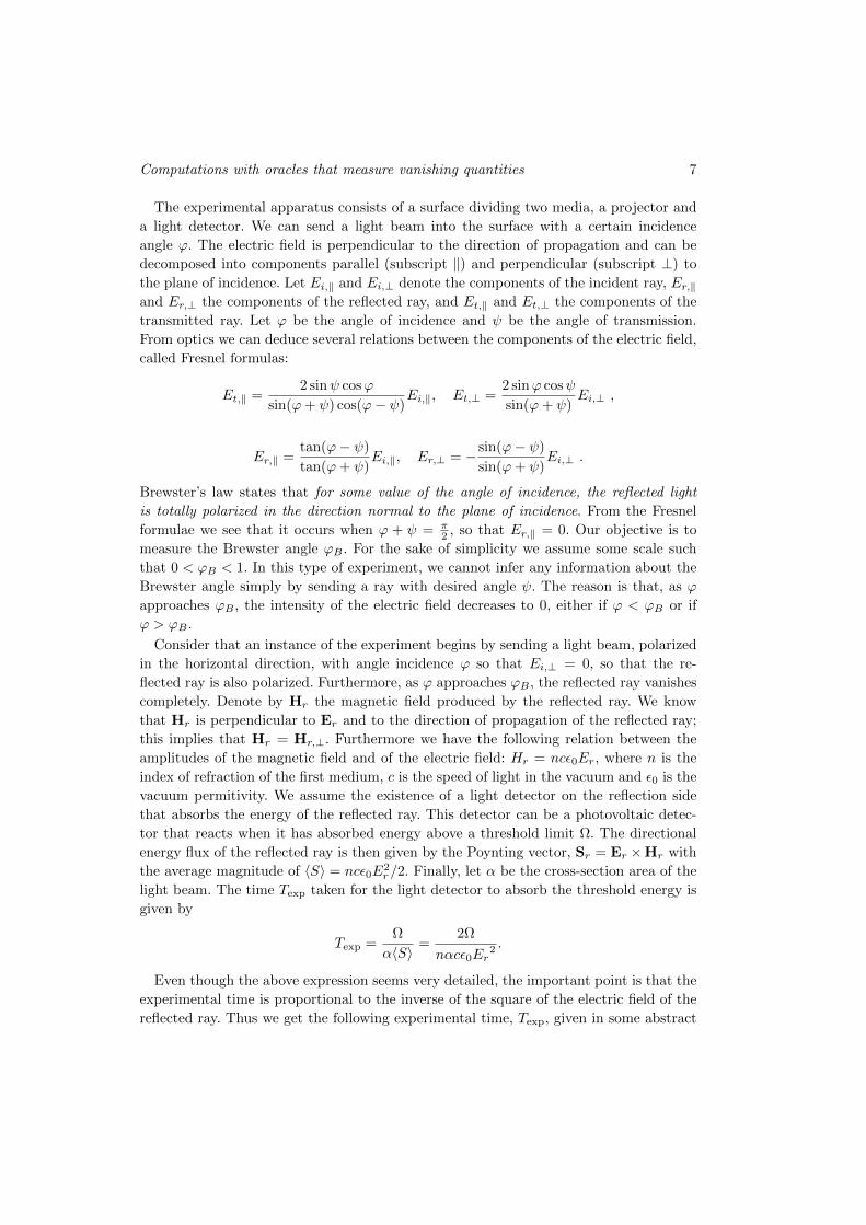
The following experiment (depicted in Figure 2) is a variation of the balance scale for
mass. The balance has two pans with a pressure stick below each pan. On the right pan
there is a body with the unknown mass of size y. To measure y we place a test mass z
on the left pan. If z = y, then the scale will not move since the lever is in equilibrium.
But, if z 6= y, then one of the pans will move down and sooner or later it will press one
of the pressure sticks. However, when z 6= y, there is no information about which of the
pans sank, only that one of them did.
z yO
Figure 2. Schematic depiction of the vanishing balance experiment.
There are also other assumptions that can be made explicit about the experiment:
(a) y is a real number in [0, 1]; (b) the mass z can be set to any dyadic rational in the
interval [0, 1]; (c) a pressure-sensitive stick is placed below each side of the balance, such
that, when one of the pans touches the pressure-sensitive stick, it reacts producing a
signal; (d) the mass z can be set so that the procedure starts from absolute rest; (e) the
friction between the masses and the pans is large enough so that these will not slide
away from their original position once the scale is in motion; and (f) the bar on which
the masses are placed is made of an homogeneous material, so that the two pans have
exactly the same weight. Assuming that the test mass weighs z and the unknown mass
weighs y, the cost of the experiment, Texp(z, y), which is the time taken for one of the
pans to touch the pressure stick, in some abstract units of time, is given by:
Texp(z, y) =
√z + y
|z − y|. (1)
This expression for the time, which exhibits an exponential growth on the precision of z
with respect to the unknown y, is typical in physical experiments, regardless the concept
being measured.
Reviewing our assumptions again, we have used the standard theory of mechanics
of rigid bodies. This means that we have neglected molecular effects, such as Coulomb
adhesion-friction, which would alter the behaviour of the system. However the purpose
Computations with oracles that measure vanishing quantities 9
of using this balance experiment is to have a generic example of a vanishing experiment,
just as in other places we had generic examples of threshold and two-sided experiments.
Note as y → z we are taking a limit of a theory of physics, and in practice another
theory may intervene, e.g., quantum mechanics. However, the case for introducing quan-
tum theory might be regarded as similar to that of imposing a general relativistic limit
on the size of a Turing machine!
3. Physical oracles and their computational power
3.1. Turing machines and physical oracles
In computability theory, after Turing and Post, an oracle for a Turing machine is accessed
by the Turing machine, which answers queries from a query tape about the membership
of elements of a set; the responses take one time step, and have no error.
A physical oracle answers queries from a query tape about the behaviour of a physical
process. In contrast to a set-theoretic oracle, it may take a variable amount of time
to answer a query – if indeed it does – and may give error prone results. The Turing
machine is connected to physical reality via a protocol. To prevent problems like the
Turing machine waiting an arbitrarily long time for a response to a query, the protocol’s
will impose a limit on waiting times.
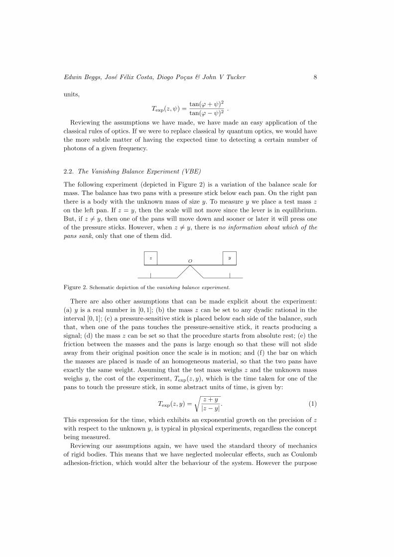
The combination of the Turing machine and physical oracle may be thought of as
having two possible functions. First, as in computability theory, information from the
physical oracle – physical observations – may be used to boost the computational power
of the Turing machine. Secondly, an innovation, the Turing machine may be used to
control some aspect of reality, such as directing a sequence of steps in an experiment or
controlling a hybrid system. In this paper we will be concerned with the first function.
The architecture is illustrated in the following diagram:
Physicalexperiment
TuringMachine
Protocolor
Interface
-
Controls experiment
Boosts computation
Consider a Turing machine running a program that queries a physical oracle via a
protocol or interface. What does the Turing machine (or its programmer) actually know?
The physical experiment itself is beyond its knowledge, it only sees queries and replies. To
study what such an augmented Turing machine can compute, we can give an axiomatic
Edwin Beggs, Jose Felix Costa, Diogo Pocas & John V Tucker 10
specification of the physical oracle, which involves a segment of physical theory and a
specification of the particular physical system that serves as the oracle.
The mathematical details of construction and operation of a Turing machine with a
physical oracle, and the key notions of precision, waiting times, timeouts etc., can be
found in the early papers of our series such as (Beggs, Costa, Loff & Tucker 2008; Beggs,
Costa, Loff & Tucker 2009; Beggs, Costa & Tucker 2012b).
One way of studying what a Turing machine with physical oracle can compute in a
given time is to use non-uniform complexity theory.
3.2. Physical oracles and non-uniform complexity classes
We consider the classical word acceptance problem for a Turing machine, but incorpo-
rating advice functions: we refer to (Balcazar, Dıas & Gabarro 1995) for advice and
non-uniform complexity, only saying what is required for understanding the this paper.
By an advice function we mean any total map f : N → Σ∗, the finite words in an
alphabet Σ; in our case, Σ is just the binary alphabet 0, 1. The pairing function is
the well known map 〈−,−〉 : Σ∗ × Σ∗ → Σ∗, computable in linear time, that allows us
to encode two words in a single word over the same alphabet by duplicating bits and
inserting a separation symbol “01”.
The definition of non-uniform complexity class follows:
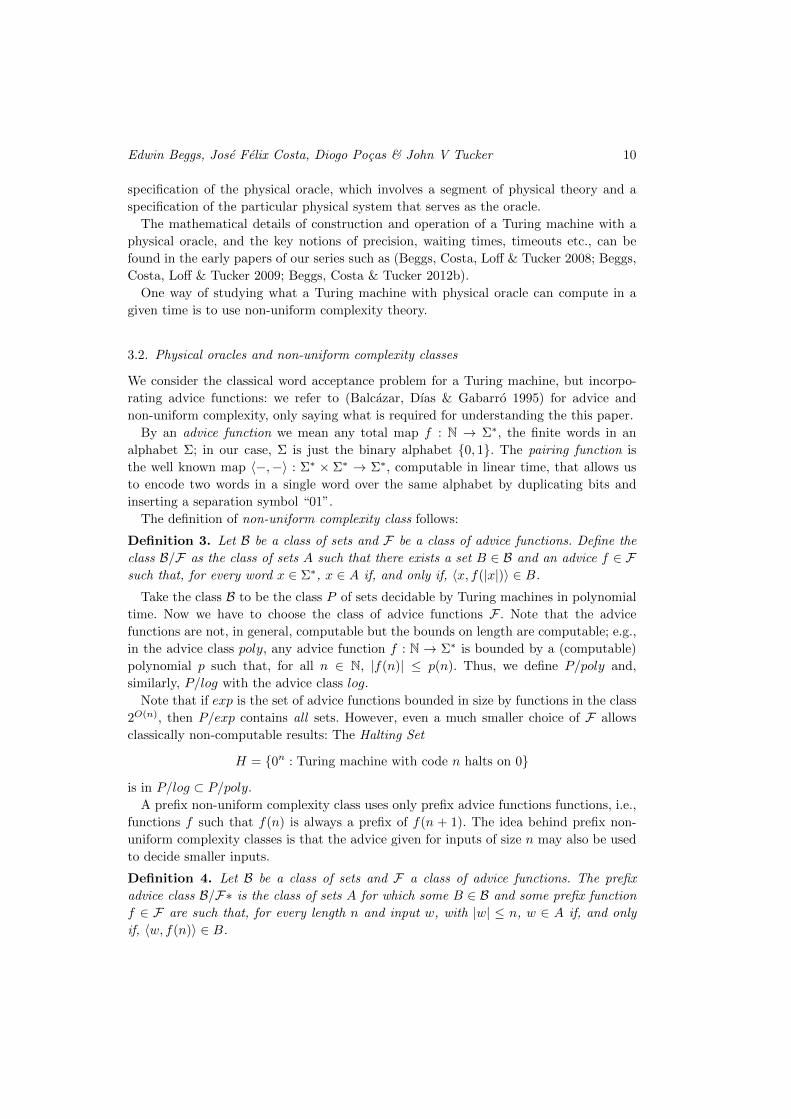
Definition 3. Let B be a class of sets and F be a class of advice functions. Define the
class B/F as the class of sets A such that there exists a set B ∈ B and an advice f ∈ Fsuch that, for every word x ∈ Σ∗, x ∈ A if, and only if, 〈x, f(|x|)〉 ∈ B.
Take the class B to be the class P of sets decidable by Turing machines in polynomial
time. Now we have to choose the class of advice functions F . Note that the advice
functions are not, in general, computable but the bounds on length are computable; e.g.,
in the advice class poly, any advice function f : N → Σ∗ is bounded by a (computable)
polynomial p such that, for all n ∈ N, |f(n)| ≤ p(n). Thus, we define P/poly and,
similarly, P/log with the advice class log.
Note that if exp is the set of advice functions bounded in size by functions in the class
2O(n), then P/exp contains all sets. However, even a much smaller choice of F allows
classically non-computable results: The Halting Set
H = 0n : Turing machine with code n halts on 0
is in P/log ⊂ P/poly.
A prefix non-uniform complexity class uses only prefix advice functions functions, i.e.,
functions f such that f(n) is always a prefix of f(n + 1). The idea behind prefix non-
uniform complexity classes is that the advice given for inputs of size n may also be used
to decide smaller inputs.
Definition 4. Let B be a class of sets and F a class of advice functions. The prefix
advice class B/F∗ is the class of sets A for which some B ∈ B and some prefix function
f ∈ F are such that, for every length n and input w, with |w| ≤ n, w ∈ A if, and only
if, 〈w, f(n)〉 ∈ B.
Computations with oracles that measure vanishing quantities 11
For probabilistic complexity classes we use the basic class BPP , which is word accep-
tance problems solvable with bounded error probability in polynomial time by a Turing
machine with access to a fair independent coin toss oracle (this might itself be consid-
ered as a form of physical oracle). Here bounded error probability means that there is a
number γ < 12 , such that the error probability of a Turing machine for any input w is
smaller than γ.
For the probabilistic complexity classes there is a complication in the definition of
BPP/F . Notice that by requiring a set B ∈ BPP and a function f ∈ F such that w ∈ Aif, and only if, 〈w, f(|w|)〉 ∈ B, we are demanding a fixed probability 1
2 + ε, 0 < ε < 12
(fixed by the Turing machine chosen to witness that B ∈ BPP ) for any possible correct
advice, instead of the more intuitive idea that the error γ = 12 −ε only has to be bounded
after choosing the correct advice. This leads to the following definitions for the specific
complexity class BPP that we will be using throughout this paper:
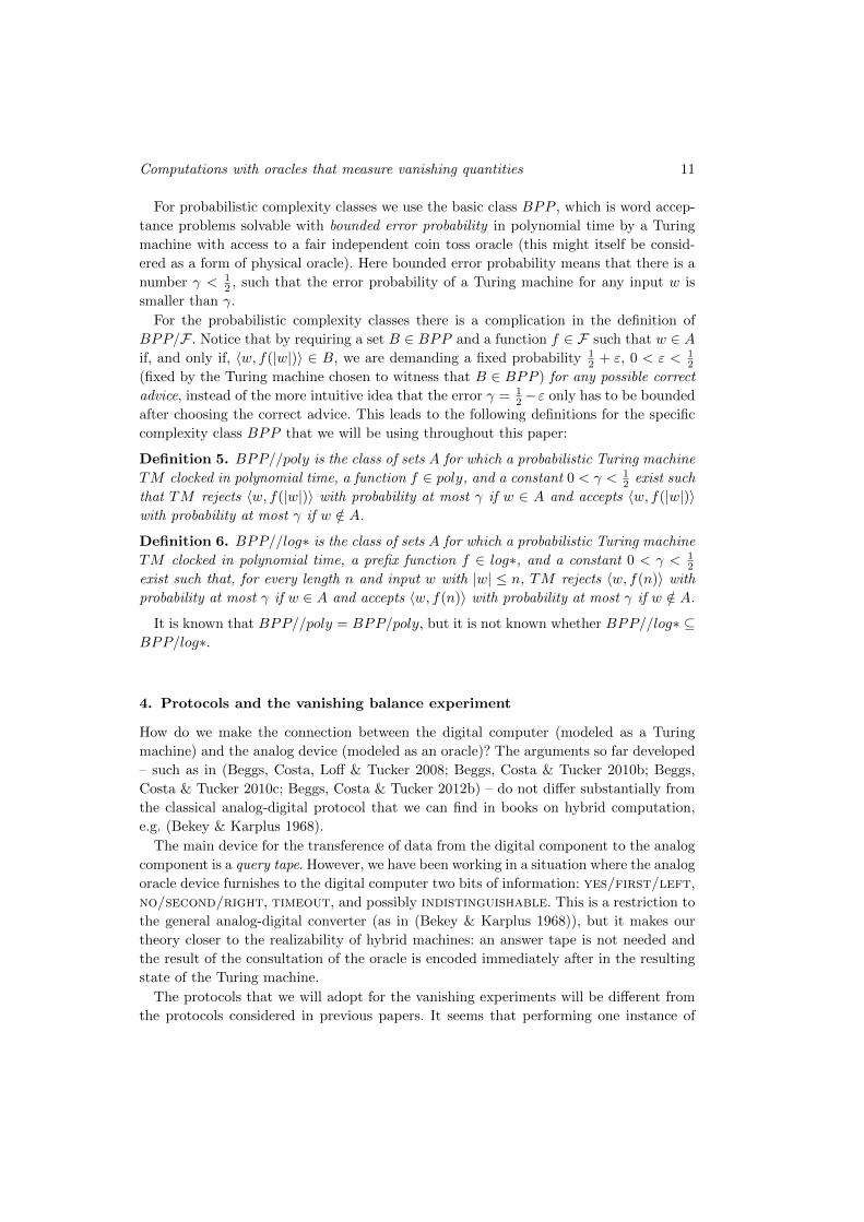
Definition 5. BPP//poly is the class of sets A for which a probabilistic Turing machine
TM clocked in polynomial time, a function f ∈ poly, and a constant 0 < γ < 12 exist such
that TM rejects 〈w, f(|w|)〉 with probability at most γ if w ∈ A and accepts 〈w, f(|w|)〉with probability at most γ if w /∈ A.
Definition 6. BPP//log∗ is the class of sets A for which a probabilistic Turing machine
TM clocked in polynomial time, a prefix function f ∈ log∗, and a constant 0 < γ < 12
exist such that, for every length n and input w with |w| ≤ n, TM rejects 〈w, f(n)〉 with
probability at most γ if w ∈ A and accepts 〈w, f(n)〉 with probability at most γ if w /∈ A.
It is known that BPP//poly = BPP/poly, but it is not known whether BPP//log∗ ⊆BPP/log∗.
4. Protocols and the vanishing balance experiment
How do we make the connection between the digital computer (modeled as a Turing
machine) and the analog device (modeled as an oracle)? The arguments so far developed
– such as in (Beggs, Costa, Loff & Tucker 2008; Beggs, Costa & Tucker 2010b; Beggs,
Costa & Tucker 2010c; Beggs, Costa & Tucker 2012b) – do not differ substantially from
the classical analog-digital protocol that we can find in books on hybrid computation,
e.g. (Bekey & Karplus 1968).
The main device for the transference of data from the digital component to the analog
component is a query tape. However, we have been working in a situation where the analog
oracle device furnishes to the digital computer two bits of information: yes/first/left,
no/second/right, timeout, and possibly indistinguishable. This is a restriction to
the general analog-digital converter (as in (Bekey & Karplus 1968)), but it makes our
theory closer to the realizability of hybrid machines: an answer tape is not needed and
the result of the consultation of the oracle is encoded immediately after in the resulting
state of the Turing machine.
The protocols that we will adopt for the vanishing experiments will be different from
the protocols considered in previous papers. It seems that performing one instance of
Edwin Beggs, Jose Felix Costa, Diogo Pocas & John V Tucker 12
the experiment does not give much information about the relationship between the test
mass z and the unknown mass y. §
We have to consider two instances of the experiment instead of one, with two differ-
ent dyadic rationals, z1 and z2 and their respective experimental times Texp(z1, y) and
Texp(z2, y). Now suppose that we can determine which of the instances of the experiment
ends first. That is, suppose that, for any two dyadic rationals, we can determine whether
Texp(z1, y) < Texp(z2, y), Texp(z1, y) = Texp(z2, y), or Texp(z1, y) > Texp(z2, y). Then we
could also determine, for a finite increasing sequence z1 < z2 < . . . < zn, which of the zicorresponds to the instance that ends last. This would then imply something about y,
thanks to the simple fact that y should be closer to dyadic rationals that consume more
experimental time. This conclusion is a consequence of the fact that Texp is increasing in
the interval [0, y) and decreasing in the interval (y, 1]. Now we ponder on the assumption
we made: given two dyadic rationals z1 and z2, corresponding to different instances of
the experiment, how can we determine which of the instances ends last? There are two
possible implementations of the experiment that can answer the question:
— To perform two experiments simultaneously, that is, to use two copies of the balance
with the same unknown mass y in the right pan. We can place masses z1 and z2at the left pans of the balances and start both experiments at the same time. If
Texp(z1, y) < Texp(z2, y), then the experiment with test mass z1 sends a first signal
and if Texp(z1, y) > Texp(z2, y), then the experiment with test mass z1 calls back first.
— Suppose we only have one balance, but now we can count the machine steps during
an experiment until the end. In this way we can begin by performing an instance of
the experiment for test mass z1, and counting the number T1 of machine transitions
that the experiment takes. Then repeat the experiment for test mass z2, obtaining a
number T2 of machine transitions. Finally, compare T1 and T2. If T1 < T2, then we
conclude that Texp(z1) < Texp(z2); if T1 > T2, then Texp(z1) > Texp(z2).
The first solution overlooks a simple practical aspect. We are basically attempting to
decide which of two events occurs first, but can we actually do it if the difference in
times becomes very small? We could answer this question in the negative, and argue
that there is a minimum time gap below which two events may appear simultaneous, so
that we cannot tell which of them happens first. The second solution also introduces a
problem. First recall that we should set a bound on the time that we consider acceptable
to wait for a response, the time schedule concept. If the experimental time exceeds the
time schedule, then the count of steps and the experiment should be interrupted. This
means that, when performing two instances of the experiment, any of them may result
in a timeout. If one experiment times out and the other does not, we can still decide
which of them ends first; nothing can be said when both experiments time out. However
§ When we were studying two-sided experiments in, say, (Beggs, Costa & Tucker 2012a) we saw that
result “left” would imply that z < y and result “right” would imply that z > y. Also, when we
were studying threshold experiments in (Beggs, Costa, Pocas & Tucker 2013a; Beggs, Costa, Pocas &Tucker 2013b) we saw that result “yes” would imply that z > y. But now, with vanishing experiments,
we only have result “yes” and this only implies that z 6= y. Of course, “timeout” should occur very
rarely, and may even not occur at all for some choices of unknown mass and time schedule.
Computations with oracles that measure vanishing quantities 13
it is not a great deal to solve this problem, since we can in principle increase the time
schedule (padding the query z with 0s) until one of the experiments ends. There is another
subtler situation in which we cannot decide which of the instances takes more time, if
the number of machine transitions is the same, that is, when T1 = T2. In this situation
the two instances are indistinguishable. Increasing the time schedule will not help, nor
will do padding 0s.
We shall use these assumptions:
— In the first implementation, we assume that we can in fact distinguish the two events
from one another. (This is, as we said, not feasible, but we are willing to consider it
because it will provide us with some interesting results later on.) In this way, when
we perform two instances of the experiment, there are three possible results: the first
instance ends first; the second instance ends first; or both instances time out;
— In the second implementation, we assume that it is possible for two experiments
to consume the same number of machine steps. In this way, when we perform two
instances of the experiment, there are four possible results: the first instance ends
first; the second instance ends first; both instances time out; or we could not decide
which instance ends first (although none of them times out).
We must also take into account the imprecision associated with placing a test mass in
the left pan. We do this in the same way as we have done in the previous papers (e.g.
(Beggs, Costa, Loff & Tucker 2008; Beggs, Costa & Tucker 2012a)), by considering three
types of precision:
(a) infinite precision (see Figures 3 and 4): when the dyadic z is read in the query
tape, a test mass z is simultaneously placed in the left pan,
(b) unbounded precision (see Figures 3 and 4): when the dyadic z is read in the query tape,
a test mass z′ is simultaneously placed in the left pan such that z−2−|z| ≤ z′ ≤ z+2−|z|
and
(c) fixed precision ε > 0 (to be discussed later on): when the dyadic z is read in the query
tape, a test mass z′ is simultaneously placed in the left pan such that z− ε ≤ z′ ≤ z+ ε.
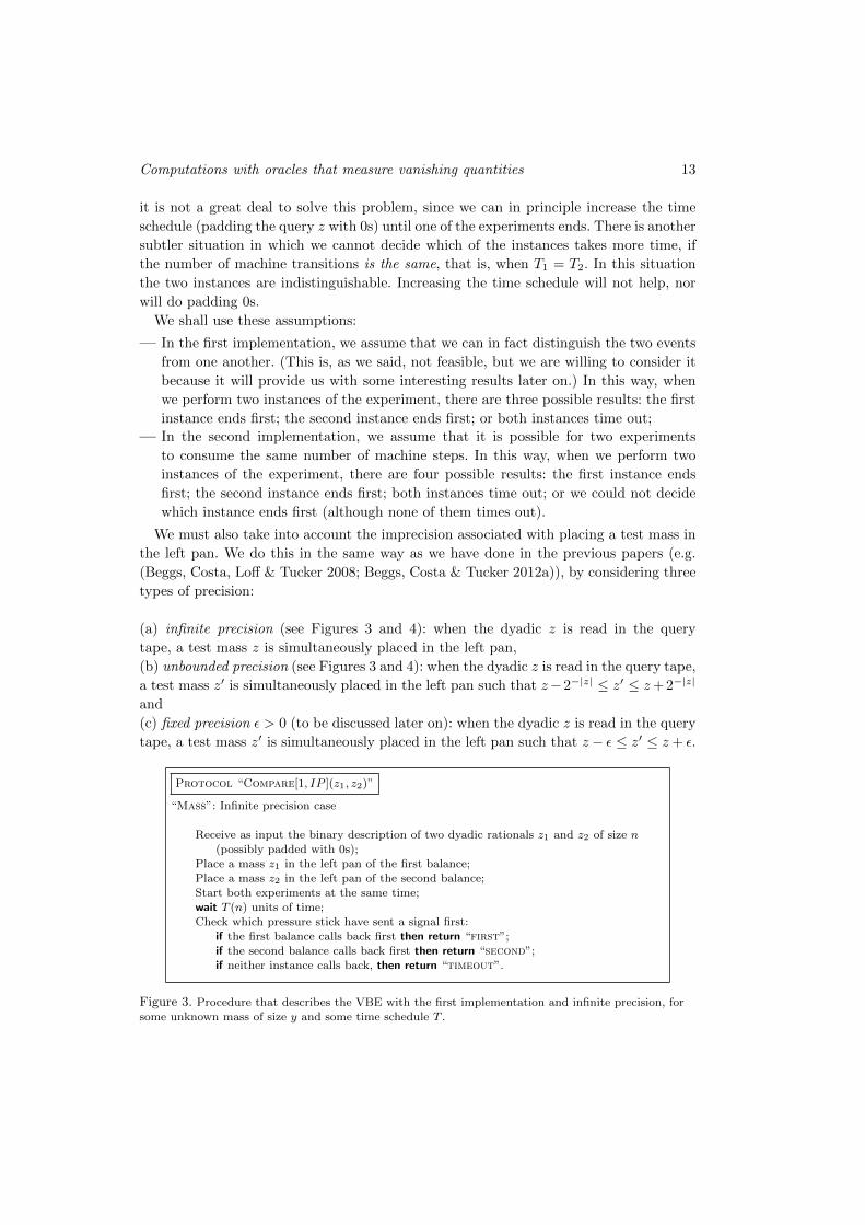
Protocol “Compare[1, IP ](z1, z2)”
“Mass”: Infinite precision case
Receive as input the binary description of two dyadic rationals z1 and z2 of size n(possibly padded with 0s);
Place a mass z1 in the left pan of the first balance;Place a mass z2 in the left pan of the second balance;Start both experiments at the same time;
wait T (n) units of time;
Check which pressure stick have sent a signal first:if the first balance calls back first then return “first”;
if the second balance calls back first then return “second”;if neither instance calls back, then return “timeout”.
Figure 3. Procedure that describes the VBE with the first implementation and infinite precision, for
some unknown mass of size y and some time schedule T .
Edwin Beggs, Jose Felix Costa, Diogo Pocas & John V Tucker 14
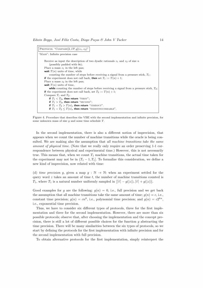
Protocol “Compare[2, IP, g](z1, z2)”
“Mass”: Infinite precision case
Receive as input the description of two dyadic rationals z1 and z2 of size n
(possibly padded with 0s);
Place a mass z1 in the left pan;wait T (n) units of time, while
counting the number of steps before receiving a signal from a pressure stick, T1;
if the experiment does not call back, then set T1 := T (n) + 1;Place a mass z2 in the left pan;
wait T (n) units of time,
while counting the number of steps before receiving a signal from a pressure stick, T2;if the experiment does not call back, set T2 := T (n) + 1;
Compare T1 and T2:if T1 < T2, then return “first”;
if T1 > T2, then return “second”;
if T1 = T2 > T (n), then return “timeout”.if T1 = T2 ≤ T (n), then return “indistinguishable”.
Figure 4. Procedure that describes the VBE with the second implementation and infinite precision, for
some unknown mass of size y and some time schedule T .
In the second implementation, there is also a different notion of imprecision, that
appears when we count the number of machine transitions while the oracle is being con-
sulted. We are making also the assumption that all machine transitions take the same
amount of physical time. (Note that we really only require an order preserving 1-1 cor-
respondence between physical and experimental time.) However, this is not necessarily
true. This means that, when we count T1 machine transitions, the actual time taken for
the experiment may not be in (T1 − 1, T1]. To formalize this consideration, we define a
new kind of imprecision, now related with time:
(d) time precision g, given a map g : N → N: when an experiment settled for the
query word z takes an amount of time t, the number of machine transitions counted is
T1, where T1 is a natural number uniformly sampled in [dte − g(|z|), dte+ g(|z|)].
Good examples for g are the following: g(n) = 0, i.e., full precision and we get back
the assumption that all machine transitions take the same amount of time; g(n) = c, i.e.,
constant time precision; g(n) = cnk, i.e., polynomial time precision; and g(n) = c2kn,
i.e., exponential time precision.
Thus, we have to consider six different types of protocols, three for the first imple-
mentation and three for the second implementation. However, there are more than six
possible protocols; observe that, after choosing the implementation and the concept pre-
cision, there is still a lot of different possible choices for the function g abstracting the
time precision. There will be many similarities between the six types of protocols, so we
start by defining the protocols for the first implementation with infinite precision and for
the second implementation with full precision.
To obtain alternative protocols for the first implementation, simply reinterpret the
Computations with oracles that measure vanishing quantities 15
instructions in Figure 3, depending on whether you are considering unbounded precision
or fixed precision ε. In the first case, we place the masses z′1 and z′2 in the left pans where
z′1 ∈ (z1− 2|z1|, z1 + 2|z1|) and z′2 ∈ (z2− 2|z2|, z2 + 2|z2|); in the second case, we consider
z′1 ∈ (z1−ε, z1+ε) and z′2 ∈ (z2−ε, z2+ε). In this way we obtain protocols Compare[1, UP ]
and Compare[1, FP (ε)]. To obtain alternate protocols for the second implementation,
simply reinterpret the instructions of the second protocol in Figure 4, depending on
whether you are considering unbounded precision or fixed precision ε. In the first case, we
place the masses z′1 and z′2 in the left pans, where z′1 ∈ (z1−2|z1|, z1+2|z1|) and z′2 ∈ (z2−2|z2|, z2+2|z2|); in the second case, we considerz′1 ∈ (z1−ε, z1+ε) and z′2 ∈ (z2−ε, z2+ε).
In this way we obtain protocols Compare[2, UP, g] and Compare[2, FP (ε), g]. Finally, the
protocols for the second implementation and different choices of time precision do not
differ, since the precision is implicitly present in counting machine transitions.
Reviewing the assumption of uniform probability densities above, we could generalise
them to some other computable probability distribution, most obviously the Gaussian
distribution. However, the uniform distribution produces simpler arguments, making the
exposition clearer, and avoids the problem of estimating the time taken to compute with
another distribution.
5. Measuring with the VBE machine with infinite precision
In what follows the suffix operation n on a word w, wn, denotes the prefix sized n of
the ω-word w0ω, no matter the size of w.
Comparing the experimental times relative to two different query words provides infor-
mation about y. Consider calls with protocol Compare[1, IP ] for input (z1, z2) such that
z1 < z2 and assume that no timeout occurs. The result of the experiment depends only
on the relationship between z1, z2 and y: (a) if y < z1 < z2, then the second experiment
will end first, (b) if z1 < y < z2, then any of the two experiments can end first, and (c) if
z1 < z2 < y, then the first experiment will end first. We can then deduce the relationship
between z1, z2 and y.
Proposition 7. Let s be the result of Compare[1, IP ](z1, z2), for an unknown mass
of size y and time schedule T , such that |z1| = |z2| = n and z1 < z2. Then, (a) if
s =“first”, then y > z1, (b) if s =“second”, then y < z2, and (c) if s =“timeout”,
then |y − z1| < 2T (|n|)−2 and |y − z2| < 2T (|n|)−2.
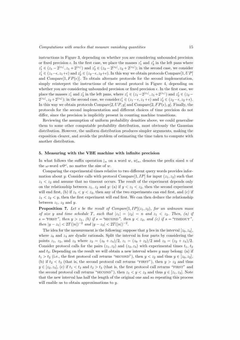
The idea for the measurement is the following: suppose that y lies in the interval [z0, z4],
where z0 and z4 are dyadic rationals. Split the interval in four parts by considering the
points z1, z2, and z3 where z2 = (z0 + z4)/2, z1 = (z0 + z2)/2 and z3 = (z2 + z4)/2.
Consider protocol calls for the pairs (z1, z2) and (z2, z3) with experimental times t1, t2and t3. Depending on the result we will obtain a new interval where y may belong: (a) if
t1 > t2 (i.e., the first protocol call returns “second”), then y < z2 and thus y ∈ [z0, z2],
(b) if t2 < t3 (that is, the second protocol call returns “first”), then y > z2 and thus
y ∈ [z2, z4], (c) if t1 < t2 and t2 > t3 (that is, the first protocol call returns “first” and
the second protocol call returns “second”), then z1 < y < z3 and thus y ∈ [z1, z3]. Note
that the new interval has half the length of the original one and so repeating this process
will enable us to obtain approximations to y.
Edwin Beggs, Jose Felix Costa, Diogo Pocas & John V Tucker 16
Algorithm “BinarySearch[1, IP ](`)”
“Mass”: Infinite precision case
input a natural number ` – number of places to the right of the left leading 0;
x0 := 0; x4 := 1; x2 := (x0 + x4)/2;
while x4 − x0 > 2−` do beginx1 := (x0 + x2)/2;
x3 := (x2 + x4)/2;
s1 := Compare[1, IP ](x1`, x2`);s2 := Compare[1, IP ](x2`, x3`);if s1 = “second” then (x0, x2, x4) := (x0, x1, x2);
else if s2 = “first” then (x0, x2, x4) := (x2, x3, x4);else if s1 = “first” and s2 = “second” then (x0, x2, x4) := (x1, x2, x3);
else if s1 = “timeout” or s2 = “timeout” then x0 := x2; x4 := x2end while;output the dyadic rational denoted by x2.
Figure 5. Procedure to obtain an approximation of an unknown mass of size y placed in the right panof the balance.
Proposition 8. For any unknown mass of size y and any time schedule T , (a) the time
complexity of the algorithm of Figure 5, for input `, is O(`T (`)), (b) for all k ∈ N, there
exists ` ∈ N such that T (`) ≥ 2(k+1)/2 and the output relative to the input ` is a dyadic
rational m such that |y −m| < 2−k, moreover, ` is at most exponential in k, and (c) if
T (k) is exponential in k, then the value of ` witnessing T (`) ≥ 2(k+1)/2 can be taken to
be linear in k.
Proposition 9. For any real number y ∈ (0, 1), the VBE machine M(y) operating with
the type I protocol with infinite precision and exponential schedule is such that: (a) for
all size n ∈ N, M(y) halts for the input word 1n and the content of the output tape is a
dyadic rational z such that |z−y| < 2−n and (b) the number of steps of M(y) is bounded
by an exponential in n.
Proof: For any y ∈ (0, 1), we take the VBE machine M(y) with unknown mass y and
any exponential time schedule T , operating with type I protocol with infinite precision.
According to Proposition 8 (b) and (c), there is a constant b such that, for all n, with
` = bn, we have that T (`) ≥ 2(n+1)/2. The machine M(y), on input 1n, just calls the
binary search procedure of Figure 5 with input ` = bn. Since T (n) is exponential in n
and ` is linear in n, the number of steps of the VBE machine, also in agreement with
Proposition 8 (a), is in O(`2a`) ⊆ O(2(a+1)`), for some a ∈ N. The next step is to provide a measurement algorithm for the type II protocol. We
will try to adapt the same algorithm, but now we have to deal with the possibility of
getting “indistinguishable”, meaning that both experimental times are too close to
separate them. To solve this problem, we compute the time differences as we approach the
unknown mass y. It would be interesting if the time differences of a protocol call increase,
i.e., if on successive calls to Compare[2, IP, g](z1, z2) the experimental time differences
would become greater. That would mean that the answer “indistinguishable” would
not occur (after some point on) and so we could deduce the position of y relative to z1
Computations with oracles that measure vanishing quantities 17
and z2. Fortunately, this is indeed true if both test masses lie on the same side relative
to y.
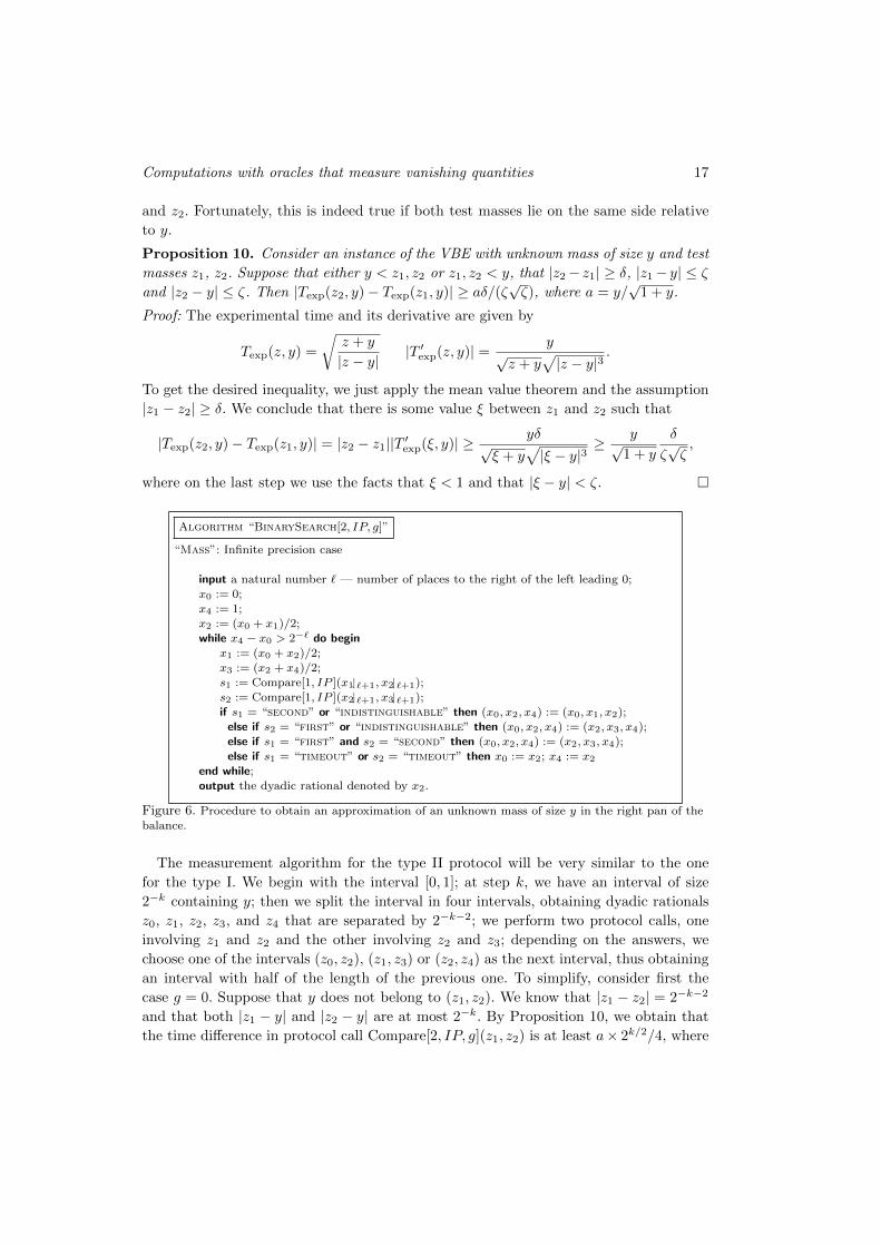
Proposition 10. Consider an instance of the VBE with unknown mass of size y and test
masses z1, z2. Suppose that either y < z1, z2 or z1, z2 < y, that |z2− z1| ≥ δ, |z1− y| ≤ ζand |z2 − y| ≤ ζ. Then |Texp(z2, y)− Texp(z1, y)| ≥ aδ/(ζ
√ζ), where a = y/
√1 + y.
Proof: The experimental time and its derivative are given by
Texp(z, y) =
√z + y
|z − y||T ′exp(z, y)| = y
√z + y
√|z − y|3
.
To get the desired inequality, we just apply the mean value theorem and the assumption
|z1 − z2| ≥ δ. We conclude that there is some value ξ between z1 and z2 such that
|Texp(z2, y)− Texp(z1, y)| = |z2 − z1||T ′exp(ξ, y)| ≥ yδ√ξ + y
√|ξ − y|3
≥ y√1 + y
δ
ζ√ζ,
where on the last step we use the facts that ξ < 1 and that |ξ − y| < ζ.
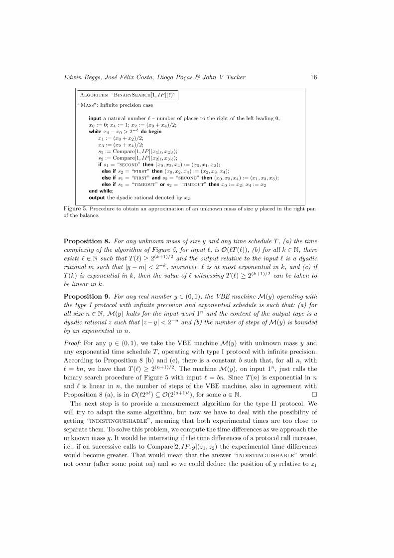
Algorithm “BinarySearch[2, IP, g]”
“Mass”: Infinite precision case
input a natural number ` — number of places to the right of the left leading 0;
x0 := 0;
x4 := 1;x2 := (x0 + x1)/2;
while x4 − x0 > 2−` do beginx1 := (x0 + x2)/2;x3 := (x2 + x4)/2;
s1 := Compare[1, IP ](x1`+1, x2`+1);
s2 := Compare[1, IP ](x2`+1, x3`+1);if s1 = “second” or “indistinguishable” then (x0, x2, x4) := (x0, x1, x2);
else if s2 = “first” or “indistinguishable” then (x0, x2, x4) := (x2, x3, x4);
else if s1 = “first” and s2 = “second” then (x0, x2, x4) := (x2, x3, x4);else if s1 = “timeout” or s2 = “timeout” then x0 := x2; x4 := x2
end while;
output the dyadic rational denoted by x2.
Figure 6. Procedure to obtain an approximation of an unknown mass of size y in the right pan of the
balance.
The measurement algorithm for the type II protocol will be very similar to the one
for the type I. We begin with the interval [0, 1]; at step k, we have an interval of size
2−k containing y; then we split the interval in four intervals, obtaining dyadic rationals
z0, z1, z2, z3, and z4 that are separated by 2−k−2; we perform two protocol calls, one
involving z1 and z2 and the other involving z2 and z3; depending on the answers, we
choose one of the intervals (z0, z2), (z1, z3) or (z2, z4) as the next interval, thus obtaining
an interval with half of the length of the previous one. To simplify, consider first the
case g = 0. Suppose that y does not belong to (z1, z2). We know that |z1 − z2| = 2−k−2
and that both |z1 − y| and |z2 − y| are at most 2−k. By Proposition 10, we obtain that
the time difference in protocol call Compare[2, IP, g](z1, z2) is at least a× 2k/2/4, where
Edwin Beggs, Jose Felix Costa, Diogo Pocas & John V Tucker 18
a is a constant. In the same way, if y does not belong to (z2, z3), the time difference
in protocol call Compare[2, IP, g](z2, z3) is at least a × 2k/2/4. We conclude that the
time difference increase exponentially step by step, which implies that we will not get
“indistinguishable” whenever the two dyadic rationals lie on the same side relative
to y. That is, if the answer to a protocol call Compare[2, IP, g](z, z′) with z < z′ is
“indistinguishable”, then z < y < z′. At step k, we make protocol calls with words
of size k + 2. Suppose that y does not lie in (z1, z2), so that the time difference is at
least a × 2k/2/4. If g = 0, then we get an answer of “first” (implying that y > z1),
“second” (implying that y < z2) or “timeout” (implying that y is very close to z1and z2). We need g to be small enough so that we do not get a wrong answer, that is,
the number of machine transitions must not differ too much from the real experimental
time. Observe that, for any g, the time differences observed (that is, the difference in
the number of machine transitions) is at least a × 2k/2/4 − 2g(k + 2). Thus, if g is
such that g(k) < a × 2k/2/16, then the imprecision in time is not enough to induce a
different answer to the protocol call. Thus, any constant time precision, polynomial time
precision, or exponential time precision g(n) = c2kn with k < 1/2 does not prejudice
our algorithm. Most of these results are asymptotic, i.e., we can only guarantee that, for
a certain point on, the time difference is great enough so that we do not get answers
of “indistinguishable”. However, in the first iterations, it is not impossible to obtain
“indistinguishable” as the answer to Compare[2, IP, g](z, z′) in a situation where y
does not belong in (z, z′). To deal with this problem, note that we could simply begin
the measurement with a subinterval of [0, 1], small enough so that it does not happen. The
specification of this subinterval only requires a finite amount of information (two dyadic
rationals of size k, for k large enough) that only depend on y and g, and thus it could
be hard-wired in the measurement algorithm. Thus, we can in fact build a measurement
algorithm for the second implementation.
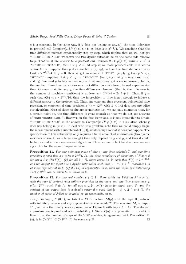
Proposition 11. For any unknown mass of size y, any time schedule T and any time
precision g such that g ∈ o(λn× 2n/2), (a) the time complexity of algorithm of Figure 6
for input ` is O(`T (`)), (b) for all k ∈ N, there exists ` ∈ N such that T (`) ≥ 2(k+1)/2
and the output for input ` is a dyadic rational m such that |y−m| < 2−k, moreover ` is
at most exponential in k, (c) if T (k) is exponential in k, then the value of ` witnessing
T (`) ≥ 2k/2 can be taken to be linear in k.
Proposition 12. For any real number y ∈ (0, 1), there exists the VBE machine M(y)
with the type II protocol with infinite precision in the mass and any time precision g ∈o(λn. 2n/2) such that: (a) for all size n ∈ N, M(y) halts for input word 1n and the
content of the output tape is a dyadic rational z such that |z − y| < 2−n and (b) the
number of steps of M(y) is bounded by an exponential in n.
Proof: For any y ∈ (0, 1), we take the VBE machine M(y) with the type II protocol
with infinite precision and any exponential time schedule T . The machine M, on input
1n, just calls the binary search procedure of Figure 6 with input ` = bn. The desired
approximation is produced with probability 1. Since T (n) is exponential in n and ` is
linear in n, the number of steps of the VBE machine, in agreement with Proposition 11
(a), is in O(`2an) ⊆ O(2(a+1)n) for some a ∈ N.
Computations with oracles that measure vanishing quantities 19
In the end of this section, we offer a different measurement algorithm for the first
implementation. We have seen that it is possible, in polynomial time, to obtain a loga-
rithmic amount of bits of the unknown mass. We will now consider other possibilities for
the measurement. For example, suppose that y > 1/2 and we want to measure the point
z > 1/2 at which Texp(z, y) = Texp(1/2, y). With type I protocol, this is indeed possible,
as the algorithm of Figure 7 suggests.
Proposition 13. Let s be a possible result of Compare[1, IP ](1`,m`) (note that 1` is
the `-bits dyadic rational 0.10 · · · 0). For any unknown mass of size y > 1/2, and r > 1/2
denote the point such that Texp(1/2, y) = Texp(r, y). Then, if s =“first”, then r ≥ m,
and, if s =“second”, then r ≤ m.
Proposition 14. For any unknown mass of size 1/2 < y <√
2/2 and any time schedule
T , let r > 1/2 denote the point such that Texp(1/2, y) = Texp(r, y). Then (a) the time
complexity of algorithm of Figure 7 for input ` is O(`T (`)) and (b) if T (`) > Texp(1/2, y),
then the output for input ` is a dyadic rational m such that |r −m| < 2−`.
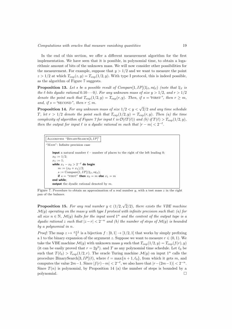
Algorithm “BinarySearch[3, IP ]”
“Mass”: Infinite precision case
input a natural number ` – number of places to the right of the left leading 0;x0 := 1/2;
x1 := 1;
while x1 − x0 > 2−` do beginm := (x0 + x1)/2;
s := Compare[1, IP ](1`,m`);if s = “first” then x0 = m else x1 = m
end while;
output the dyadic rational denoted by m.
Figure 7. Procedure to obtain an approximation of a real number y, with a test mass z in the right
pan of the balance.
Proposition 15. For any real number y ∈ (1/2,√
2/2), there exists the VBE machine
M(y) operating on the mass y with type I protocol with infinite precision such that: (a) for
all size n ∈ N, M(y) halts for the input word 1n and the content of the output tape is a
dyadic rational z such that |z−r| < 2−n and (b) the number of steps of M(y) is bounded
by a polynomial in n.
Proof: The map z 7→ z+12 is a bijection f : [0, 1]→ [1/2, 1] that works by simply prefixing
a 1 to the binary expansion of the argument z. Suppose we want to measure r ∈ (0, 1). We
take the VBE machineM(y) with unknown mass y such that Texp(1/2, y) = Texp(f(r), y)
(it can be easily proved that r = 2y2). and T as any polynomial time schedule. Let `0 be
such that T (`0) > Texp(1/2, r). The oracle Turing machine M(y) on input 1n calls the
procedure BinarySearch[3, IP ](`), where ` = maxn+ 1, `0, from which it gets m, and
computes the value 2m−1. Since |f(r)−m| < 2−`, we also have that |r−(2m−1)| < 2−n.
Since T (n) is polynomial, by Proposition 14 (a) the number of steps is bounded by a
polynomial.
Edwin Beggs, Jose Felix Costa, Diogo Pocas & John V Tucker 20
6. Measuring with the VBE machine with unbounded precision
The measuring algorithm provided for protocol of type I operating with unbounded
precision is very similar to algorithm BinarySearch[3, IP ]. Its goal is again to measure
the value r > 1/2 for which Texp(1/2, y) = Texp(r, y), where y is the “unknown mass”.
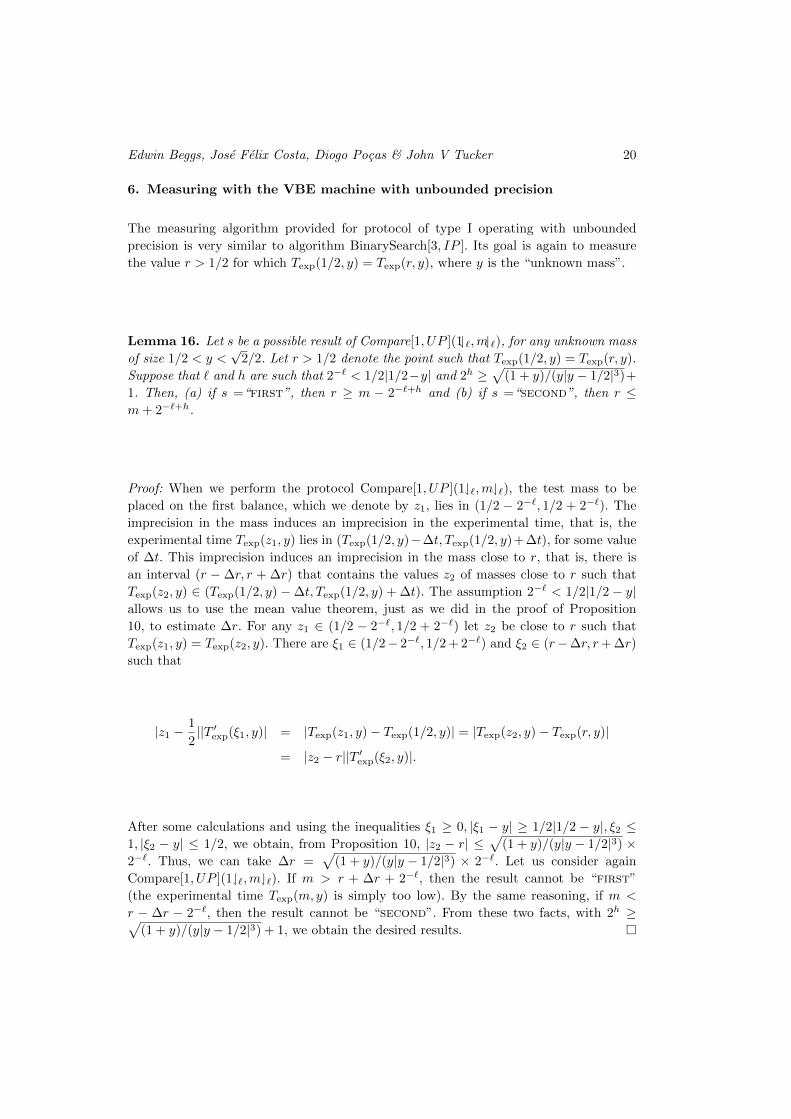
Lemma 16. Let s be a possible result of Compare[1, UP ](1`,m`), for any unknown mass
of size 1/2 < y <√
2/2. Let r > 1/2 denote the point such that Texp(1/2, y) = Texp(r, y).
Suppose that ` and h are such that 2−` < 1/2|1/2−y| and 2h ≥√
(1 + y)/(y|y − 1/2|3)+
1. Then, (a) if s =“first”, then r ≥ m − 2−`+h and (b) if s =“second”, then r ≤m+ 2−`+h.
Proof: When we perform the protocol Compare[1, UP ](1`,m`), the test mass to be
placed on the first balance, which we denote by z1, lies in (1/2 − 2−`, 1/2 + 2−`). The
imprecision in the mass induces an imprecision in the experimental time, that is, the
experimental time Texp(z1, y) lies in (Texp(1/2, y)−∆t, Texp(1/2, y)+∆t), for some value
of ∆t. This imprecision induces an imprecision in the mass close to r, that is, there is
an interval (r − ∆r, r + ∆r) that contains the values z2 of masses close to r such that
Texp(z2, y) ∈ (Texp(1/2, y) −∆t, Texp(1/2, y) + ∆t). The assumption 2−` < 1/2|1/2 − y|allows us to use the mean value theorem, just as we did in the proof of Proposition
10, to estimate ∆r. For any z1 ∈ (1/2 − 2−`, 1/2 + 2−`) let z2 be close to r such that
Texp(z1, y) = Texp(z2, y). There are ξ1 ∈ (1/2− 2−`, 1/2 + 2−`) and ξ2 ∈ (r−∆r, r+ ∆r)
such that
|z1 −1
2||T ′exp(ξ1, y)| = |Texp(z1, y)− Texp(1/2, y)| = |Texp(z2, y)− Texp(r, y)|
= |z2 − r||T ′exp(ξ2, y)|.
After some calculations and using the inequalities ξ1 ≥ 0, |ξ1 − y| ≥ 1/2|1/2 − y|, ξ2 ≤1, |ξ2 − y| ≤ 1/2, we obtain, from Proposition 10, |z2 − r| ≤
√(1 + y)/(y|y − 1/2|3) ×
2−`. Thus, we can take ∆r =√
(1 + y)/(y|y − 1/2|3) × 2−`. Let us consider again
Compare[1, UP ](1`,m`). If m > r + ∆r + 2−`, then the result cannot be “first”
(the experimental time Texp(m, y) is simply too low). By the same reasoning, if m <
r − ∆r − 2−`, then the result cannot be “second”. From these two facts, with 2h ≥√(1 + y)/(y|y − 1/2|3) + 1, we obtain the desired results.
Computations with oracles that measure vanishing quantities 21
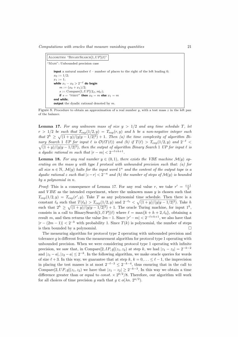
Algorithm “BinarySearch[1, UP ](`)”
“Mass”: Unbounded precision case
input a natural number ` – number of places to the right of the left leading 0;
x0 := 1/2;
x1 := 1;while x1 − x0 > 2−` do begin
m := (x0 + x1)/2;
s := Compare[1, UP ](1`,m`);if s = “first” then x0 = m else x1 = m
end while;output the dyadic rational denoted by m.
Figure 8. Procedure to obtain an approximation of a real number y, with a test mass z in the left pan
of the balance.
Lemma 17. For any unknown mass of size y > 1/2 and any time schedule T , let
r > 1/2 be such that Texp(1/2, y) = Texp(r, y) and h be a non-negative integer such
that 2h ≥√
(1 + y)/(y|y − 1/2|3) + 1. Then (a) the time complexity of algorithm Bi-
nary Search 1 UP for input ` is O(`T (`)) and (b) if T (`) > Texp(1/2, y) and 2−` <√(1 + y)/(y|y − 1/2|3), then the output of algorithm Binary Search 1 UP for input ` is
a dyadic rational m such that |r −m| < 2−`+h+1.
Lemma 18. For any real number y ∈ (0, 1), there exists the VBE machine M(y) op-
erating on the mass y with type I protocol with unbounded precision such that: (a) for
all size n ∈ N, M(y) halts for the input word 1n and the content of the output tape is a
dyadic rational z such that |z−r| < 2−n and (b) the number of steps of M(y) is bounded
by a polynomial in n.
Proof: This is a consequence of Lemma 17. For any real value r, we take r′ = r+12
and V BE as the intended experiment, where the unknown mass y is chosen such that
Texp(1/2, y) = Texp(r′, y). Take T as any polynomial time schedule. Then there is a
constant `0 such that T (`0) > Texp(1/2, y) and 2−`0 <√
(1 + y)/(y|y − 1/2|3). Take h
such that 2h ≥√
(1 + y)/(y|y − 1/2|3) + 1. The oracle Turing machine, for input 1k,
consists in a call to BinarySearch[1, UP ](`) where ` = maxk + h + 2, `0, obtaining a
result m, and then returns the value 2m−1. Since |r′−m| < 2−`+h+1, we also have that
|r − (2m − 1)| < 2−k with probability 1. Since T (k) is polynomial, the number of steps
is then bounded by a polynomial. The measuring algorithm for protocol type 2 operating with unbounded precision and
tolerance g is different from the measurement algorithm for protocol type 1 operating with
unbounded precision. When we were considering protocol type 1 operating with infinite
precision, we saw that, in Compare[2, IP, g](z1, z2) at step k, we had |z1 − z2| = 2−k−2
and |z1− a|, |z2− a| ≤ 2−k. In the following algorithm, we make oracle queries for words
of size `+ 3. In this way, we guarantee that at step k, k = 0, . . . ≤ `− 1, the imprecision
in placing the test masses is at most 2−`−3 ≤ 2−k−4, thus ensuring that in the call to
Compare[2, UP, g](z1, z2) we have that |z1 − z2| ≥ 2−k−3. In this way we obtain a time
difference greater than or equal to const. × 2k/2/8. Therefore, our algorithm will work
for all choices of time precision g such that g ∈ o(λn. 2n/2).
Edwin Beggs, Jose Felix Costa, Diogo Pocas & John V Tucker 22
Algorithm “BinarySearch[2, UP, g](`)”
“Mass”: Unbounded precision case
input a natural number ` — number of places to the right of the left leading 0;
x0 := 0;
x4 := 1;x2 := (x0 + x1)/2;
while x4 − x0 > 2−` do beginx1 := (x0 + x2)/2;x3 := (x2 + x4)/2;
s1 := Compare[2, UP, g](x1`+3, x2`+3);
s2 := Compare[2, UP, g](x2`+3, x3`+3);if s1 = “second” or “indistinguishable” then (x0, x2, x4) := (x0, x1, x2);
else if s2 = “first” or “indistinguishable” then (x0, x2, x4) := (x2, x3, x4);
else if s1 = “first” and s2 = “second” then (x0, x2, x4) := (x2, x3, x4);else if s1 = “timeout” or s2 = “timeout” then x0 := x2; x4 := x2
end while;
output the dyadic rational denoted by x2.
Figure 9. Procedure to obtain an approximation of an unknown mass y in the right pan of the balance.
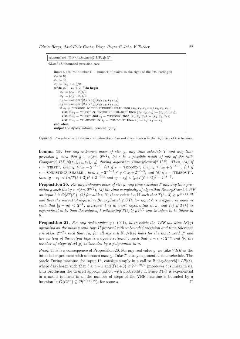
Lemma 19. For any unknown mass of size y, any time schedule T and any time
precision g such that g ∈ o(λn. 2n/2), let s be a possible result of one of the calls
Compare[2, UP, g](z1 `+3, z2 `+3) during algorithm BinarySearch[2, UP ]. Then, (a) if
s =“first”, then y ≥ z1 − 2−`−3, (b) if s =“second”, then y ≤ z2 + 2−`−3, (c) if
s =“undistinguishable”, then z1−2−`−3 ≤ y ≤ z2 +2−`−3, and (d) if s =“timeout”,
then |y − z1| < (µ/T (`+ 3))2 + 2−`−3 and |y − z2| < (µ/T (`+ 3))2 + 2−`−3.
Proposition 20. For any unknown mass of size y, any time schedule T and any time pre-
cision g such that g ∈ o(λn. 2n/2), (a) the time complexity of algorithm BinarySearch[2, UP ]
on input ` is O(`T (`)), (b) for all k ∈ N, there exists ` ∈ N such that T (`+3) ≥ µ2(k+1)/2
and thus the output of algorithm BinarySearch[2, UP ] for input ` is a dyadic rational m
such that |y − m| < 2−k, moreover ` is at most exponential in k, and (c) if T (k) is
exponential in k, then the value of ` witnessing T (`) ≥ µ2k/2 can be taken to be linear in
k.
Proposition 21. For any real number y ∈ (0, 1), there exists the VBE machine M(y)
operating on the mass y with type II protocol with unbounded precision and time tolerance
g ∈ o(λn. 2n/2) such that: (a) for all size n ∈ N, M(y) halts for the input word 1n and
the content of the output tape is a dyadic rational z such that |z − r| < 2−n and (b) the
number of steps of M(y) is bounded by a polynomial in n.
Proof: This is a consequence of Proposition 20. For any real value y, we take V BE as the
intended experiment with unknown mass y. Take T as any exponential time schedule. The
oracle Turing machine, for input 1n, consists simply in a call to BinarySearch[1, IP ](`),
where ` is chosen such that ` ≥ n+ 1 and T (`+ 3) ≥ 2(n+2)/2 (moreover ` is linear in n),
thus producing the desired approximation with probability 1. Since T (n) is exponential
in n and ` is linear in n, the number of steps of the VBE machine is bounded by a
function in O(`2an) ⊆ O(2(a+1)n), for some a.
Computations with oracles that measure vanishing quantities 23
7. Measuring with the VBE machine with fixed precision
The final case to consider is that of fixed precision. The measurement algorithms that we
are going to specify do not produce approximations to a given mass. Instead, the goal is to
compute the approximation to the probability of some particular event. We are going to
obtain approximations to the probability of getting “first” from Compare[...](10`, 11`),corresponding to the test masses 1/2 and 3/4, with fixed precision ε for the mass and
time tolerance g, either in the type I or type II protocols.
Proposition 22. Let T be a time schedule such that T (2) > Texp(1/2, 3/4) =√
5.
For any mass y ∈ (1/2, 3/4), let Pfirst(y) denote the probability of obtaining result
“first” in protocol Compare [1, FP (ε)](10, 11) (resp. Compare[2, FP (ε), g](10, 11), for
any time tolerance g) for the experiment with test mass y. Then, for any sufficiently
small ε, Pfirst(1/2) = 0, Pfirst(3/4) = 1 and Pfirst is a continuous, increasing function
in (1/2, 3/4).
The above proposition entails that, by the intermediate value theorem, for any intended
probability p, there is some mass y such that Pfirst(y) = p, and so we can compute
approximations to p by setting y as desired and repeating several times the protocol call
Compare[...](10, 11). All that is left is to formalize the algorithm and state its properties.
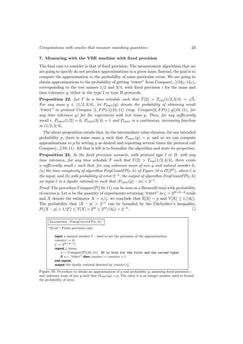
Proposition 23. In the fixed precision scenario, with protocol type I or II, with any
time tolerance, for any time schedule T such that T (2) > Texp(1/2, 3/4), there exists
a sufficiently small ε such that, for any unknown mass of size y and natural number h,
(a) the time complexity of algorithm FreqCountFP(ε, h) of Figure 10 is O(22`), where ` is
the input, and (b) with probability of error 2−h, the output of algorithm FreqCountFP(ε, h)
on input ` is a dyadic rational m such that |Pfirst(y)−m| < 2−`.
Proof: The procedure Compare[P](10, 11) can be seen as a Bernoulli trial with probability
of success p. Let α be the quantity of experiments returning “first” in ζ = 22`+h−2 trials
and X denote the estimator X = α/ζ. we conclude that E[X] = p and V[X] ≤ 1/(4ζ).
The probability that |X − p| > 2−` can be bounded by the Chebyshev’s inequality,
P (|X − p| > 1/2`) ≤ V[X]× 22` ≤ 22`/(4ζ) = 2−h.
Algorithm “FreqCountFP(ε, h)”
“Mass”: Finite precision case
input a natural number ` – used to set the precision of the approximation;counter := 0;
ζ := 22`+h−2;
repeat ζ timess := Compare[P](10, 11); %P is both for the first and the second types
if s = “first” then counter := counter + 1
end repeat;output the dyadic rational denoted by counter/ζ.
Figure 10. Procedure to obtain an approximation of a real probability p, assuming fixed precision ε
and unknown mass of size y such that Pfirst(y) = p. The value h is an integer number used to boundthe probability of error.
Edwin Beggs, Jose Felix Costa, Diogo Pocas & John V Tucker 24
Proposition 24. For any real number y ∈ (0, 1), for all sufficiently small ε, and for all
γ ∈ (0, 1/2), there exists the VBE machine M(y) clocked in exponential time operating,
either with type I protocol or type II protocol with arbitrary tolerance, with fixed precision
ε, such that, for every n ∈ N, every computation of M(y) on input word 1n halts with a
dyadic rational z as output, such that, with probability of failure at most γ, |z−r| < 2−n.
Proof: This is a consequence of Proposition 23. We take any time schedule T such that
T (2) > Texp(1/2, 3/4), any ε ∈ (0, 1/2) in the conditions of Proposition 22 and, for
any γ ∈ (0, 1), any positive integer number h such that 2−h ≤ γ. Now consider the
oracle Turing machine that, for input word 1`, makes a call to FreqCountFP(ε, h)(`). For
any real number r we take the VBE machine with unknown mass y chosen such that
Pfirst(y) = r, where Pfirst is given by Proposition 22. The above machine produces the
desired approximation with probability of failure at most 2−h ≤ γ. Furthermore, the
number of steps is bounded by a function of the order of O(22`).
8. Tossing coins with the VBE machine
The final step before establishing lower bounds is to find out which protocols can be used
with the VBE to simulate coin tosses. As expected, any probabilistic protocol suffices;
that is, only Type I and Type II protocols operating with infinite precision and infinite
precision and tolerance 0, respectively, do not allow for fair coin tosses.
Proposition 25. The VBE machine operating with type I protocol with unbounded or
fixed precision for sufficiently small ε can simulate arbitrarily long sequences of fair in-
dependent coin tosses, to within a specified chance of failure.
Proof: For a given y, let z be a dyadic rational such that z 6= y and let ` ≥ |z| be
such that T (`) > Texp(z, y). Observe that both calls Compare[..., UP, ...](z`, z`) and
Compare[..., FP (ε), ...](z`, z`) have more than one possible result (in fact, both return
“first” or “second” with the same, non-null probability).
Proposition 26. The VBE machine operating with type II protocol with infinite, un-
bounded, or fixed precision, for sufficiently small ε and non-null tolerance g, permits coin
tosses.
Proof: For a given y, let z be a dyadic rational such that z 6= y and let ` ≥ |z| be such that
T (`) > Texp(z, y) and g(`) > 0. Now observe that protocol call Compare[2, P, g](z`, z`),where P is any of the protocol variants, has more than one possible result (in fact, both
return “first” or “second” with the same, non-null probability).
Proposition 27. The VBE machine operating with type II protocol with unbounded or
fixed precision, for sufficiently small ε and tolerance 0, permits coin tosses.
Proof: For a given unknown mass y, we will find a dyadic rational z of size ` such that
the protocol call Compare[2, UP, 0](z`, z`) (resp. Compare[2, FP (ε), 0](z`, z`)) returns
“first” or “second” with the same probability. We will require that T (`) > Texp(z, y)
(this ensures that we do not get “timeout” with probability 1) and dTexp(z−2−`, y)e 6=dTexp(z + 2−`, y)e (resp. dTexp(z − ε, y)e 6= dTexp(z + ε, y)e; this ensures that we do not
get “undistinguishable” with probability 1). The above constraints are satisfied by
Computations with oracles that measure vanishing quantities 25
considering a large enough integer k such that equation Texp(x, y) = k, for fixed y, has a
solution x. We then take ` such that T (`) > k and z of size ` such that z − 2−` < x ≤ z(resp. z − ε < x ≤ z).
9. Encoding discrete functions as real numbers
Denote the Cantor numbers by C3, the set of real numbers x such that x =∑∞k=1 xk2−3k,
where xk ∈ 1, 2, 4, i.e., the numbers composed by triples of the form 001, 010, or 100.
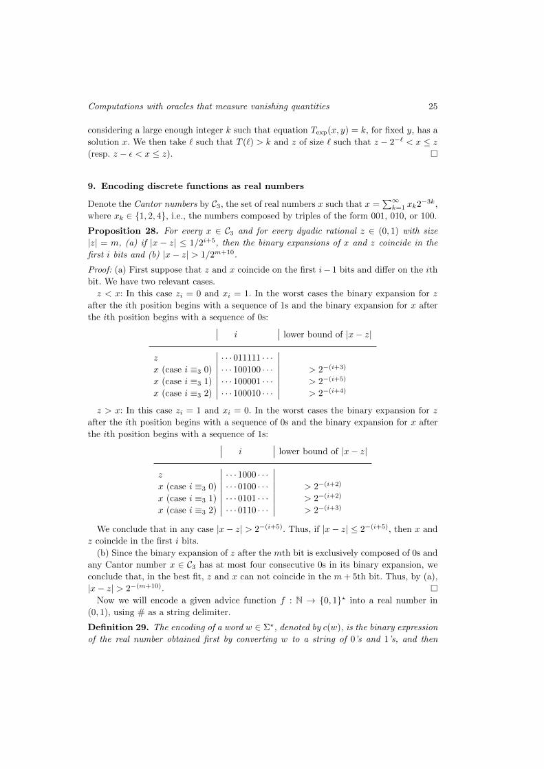
Proposition 28. For every x ∈ C3 and for every dyadic rational z ∈ (0, 1) with size
|z| = m, (a) if |x − z| ≤ 1/2i+5, then the binary expansions of x and z coincide in the
first i bits and (b) |x− z| > 1/2m+10.
Proof: (a) First suppose that z and x coincide on the first i− 1 bits and differ on the ith
bit. We have two relevant cases.
z < x: In this case zi = 0 and xi = 1. In the worst cases the binary expansion for z
after the ith position begins with a sequence of 1s and the binary expansion for x after
the ith position begins with a sequence of 0s:
i lower bound of |x− z|
z · · · 011111 · · ·x (case i ≡3 0) · · · 100100 · · · > 2−(i+3)
x (case i ≡3 1) · · · 100001 · · · > 2−(i+5)
x (case i ≡3 2) · · · 100010 · · · > 2−(i+4)
z > x: In this case zi = 1 and xi = 0. In the worst cases the binary expansion for z
after the ith position begins with a sequence of 0s and the binary expansion for x after
the ith position begins with a sequence of 1s:
i lower bound of |x− z|
z · · · 1000 · · ·x (case i ≡3 0) · · · 0100 · · · > 2−(i+2)
x (case i ≡3 1) · · · 0101 · · · > 2−(i+2)
x (case i ≡3 2) · · · 0110 · · · > 2−(i+3)
We conclude that in any case |x− z| > 2−(i+5). Thus, if |x− z| ≤ 2−(i+5), then x and
z coincide in the first i bits.
(b) Since the binary expansion of z after the mth bit is exclusively composed of 0s and
any Cantor number x ∈ C3 has at most four consecutive 0s in its binary expansion, we
conclude that, in the best fit, z and x can not coincide in the m+ 5th bit. Thus, by (a),
|x− z| > 2−(m+10). Now we will encode a given advice function f : N → 0, 1? into a real number in
(0, 1), using # as a string delimiter.
Definition 29. The encoding of a word w ∈ Σ?, denoted by c(w), is the binary expression
of the real number obtained first by converting w to a string of 0’s and 1’s, and then
Edwin Beggs, Jose Felix Costa, Diogo Pocas & John V Tucker 26
replacing every 0 by 100 and every 1 by 010. Given a function f ∈ log?, we denote the
encoding of f by the real number µ(f) = limµ(f)(n), recursively defined by (a) µ(f)(0) =
0 · c(f(0)), (b) µ(f)(n+ 1) = µ(f)(n)#c(s) whenever f(n+ 1) = f(n)#s and n+ 1 is not
a power of two, and (c) µ(f)(n+ 1) = µ(f)(n)#c(s)#001, whenever f(n+ 1) = f(n)#s
and n+ 1 is a power of two.
The encoding above consists on replacing the bits of f by triples 100 and 010, adding
001 at the end of each code of f(2k), with k ∈ N. Observe that, by construction, µ(f) ∈ C3.
Also, from the encoding we need to get back values of the advice f . To obtain f(2k),
we just have to read the bits of µ(f) in triples until the (k + 1)-th triple 001 is found.
Consequently, one may say that, whenever f ∈ log?, by knowing O(k) bits of the real
number µ(f), we can know f(2k).
Bounds similar to those in the proposition above have other uses – compare the role
of Proposition 3.5 in the continuity studies in (Pauly & Zeigler 2013).
10. Lower bounds on the computational power of the VBE machine
We studied all variety of protocols sufficiently enough to prove the following theorems.
Proposition 30. If A ∈ P/poly, then A is decidable in polynomial time by the VBE
machine M(y) for some suitable y operating with type I protocol using infinite precision.
Proof: This proof of this proposition follows the steps of Proposition 32, mutatis mutandis.
Proposition 31. (a) If A ∈ P/poly, then A is decidable in polynomial time by the
VBE machine M(y) for some suitable y operating with type I protocol using unbounded
precision. (b) If A ∈ BPP//log?, then A is decidable in polynomial time by the VBE
machine operating with type I protocol and sufficiently small fixed precision ε.
Proof: This proof of this proposition follows the steps of Proposition 33, mutatis mutandis,
noting that P/poly = BPP//poly .
Proposition 32. If A ∈ P/log?, then A is decidable in polynomial time by the VBE
machine M(y) for some suitable y operating with type II protocol using infinite precision
and tolerance zero.
Proof: Let f be a prefix function in log andM be a Turing machine running in polynomial
time such that, for every n ∈ N and every word w of size less than or equal to n, w ∈ Aif and only if M accepts 〈w, f(n)〉. Take y to be the encoding of f as a real number in
(0, 1). According with Proposition 12, there exists an integer k, an oracle Turing machine
M′(y) and a time schedule T , such that (a) for every n ∈ N, M′(y) on input 1n halts
and outputs the dyadic rational z such that |z − r| < 2−n and (b) the number of steps
ofM′(y) is bounded by a function in 2O(n). Our next step is to define the oracle Turing
machine,M′′(y), that decides A. For a given input w of size n, we perform a sequence of
experiments to compute f(n′), for some n′ > n. We take n′ = 2dlog(n)e. In this way, we
can obtain f(n′) if we know the binary expansion of y up to the (dlog(n)e+ 1)-th triple
of the form 001.
Since f ∈ log, this means that there are constants a and b such that, for all n, |f(n)| ≤

Computations with oracles that measure vanishing quantities 27
a log(n) + b. In particular, |f(n′)| ≤ adlog(n)e + b. Thus, we need to know at most the
first 3(adlog(n)e + b) + 3(dlog(n)e + 1) bits of the binary expansion of y to get to the
desired triple 001. Finally, we specify our VBE machine, M′′(y) using time schedule T .
For a given input word w of size n, it simulates the machine M′(y) for input 1`, where
` = 3(a+1)dlog(n)e+3b+8. By the discussion above, the result is a dyadic rational z such
that |z−r| < 2−` and thus z and r coincide in the first `−5 = 3(a+1)dlog(n)e+3(b+1)
bits, and so z can be used to decode f(n′). Afterwards, simulate M for the input word
〈w, f(n′)〉 and accept or reject based on the result of the simulation. It is clear that this
machine decides A. The time complexity of the simulation ofM′(y) is O(2a`). Since ` is
logarithmic on n, the result is polynomial in n. And since M runs in polynomial time,
we conclude that M′′(y) also runs in polynomial time.
Proposition 33. (a) If A ∈ BPP//log?, then A is decidable in polynomial time by the
VBE machine operating with type II protocol with unbounded precision and time tolerance
g ∈ o(λn.2n/2). (b) If A ∈ BPP//log?, then A is decidable in polynomial time by the
VBE machine operating with type II protocol with sufficiently small fixed precision and
any time tolerance.
Proof: We prove for the case of unbounded precision. The proof relative to the fixed
precision case is similar. We use a proof similar to the proof of Proposition 32, but now
we have to take into account both the error probability in measuring and the simulation
of a fair coin toss.
Let f be a prefix function in log, γ1 be a real number in (0, 1/2) and N be a Turing
machine running in polynomial time such that, for any natural number n and any word
w of size less than or equal to n,
if w ∈ A, then N rejects 〈w, f(n)〉 with probability at most γ1;
if w 6∈ A, then N accepts 〈w, f(n)〉 with probability at most γ1.
Let p3 be a polynomial bound on the running time of N . Let also r be the coding
y = µ(f) and γ3 be such that γ1 + γ3 < 1/2. Then, according with Propositions 21
(unbounded precision) and 24 (fixed precision), there is an integer k, an oracle Turing
machineM(y), and a time schedule T such that: (a) for all size n, every computation of
M(y), for input word 1n, halts and, with probability of failure at most γ3, the content
of the output tape is a dyadic rational z such that |z − y| < 2−n and (b) the number of
steps of M(y) is bounded by a function in O(2an).
Furthermore, in agreement with Propositions 26 or 27, we conclude that there is a
dyadic rational z such that the protocol call with query z has more than one possible
result with non-null probability. This means that protocol call has a probability of δ of
producing some result r1, with δ ∈ (0, 1). Let also γ2 be a positive real number such
that γ1 + γ2 + γ3 < 1/2. There is an integer K (depending on δ and γ2) such that, for
all n, we can use Kn independent biased coin tosses to simulate n fair coin tosses, with
probability of failure at most γ2.
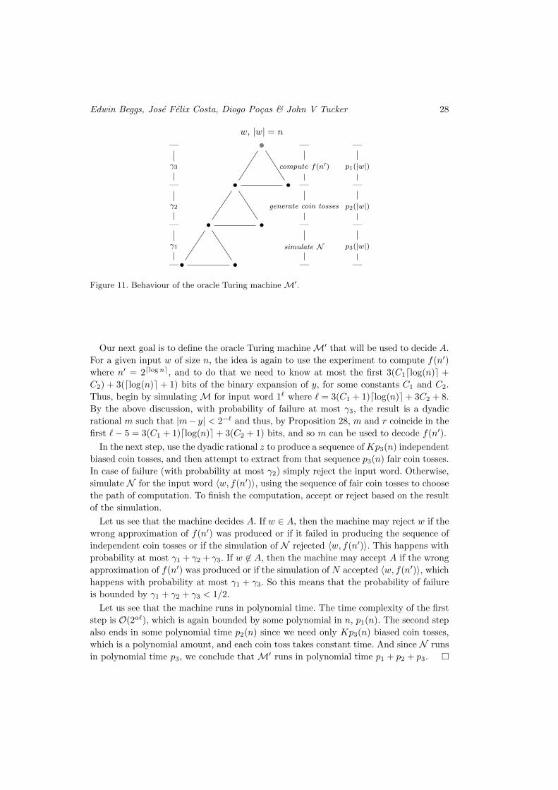
Edwin Beggs, Jose Felix Costa, Diogo Pocas & John V Tucker 28
•
• •
• •
• •
—
compute f(n′)
—
generate coin tosses
—
simulate N
—
—
p1(|w|)
—
p2(|w|)
—
p3(|w|)
—
—
γ3
—
γ2
—
γ1
—
w, |w| = n
Figure 11. Behaviour of the oracle Turing machine M′.
Our next goal is to define the oracle Turing machineM′ that will be used to decide A.
For a given input w of size n, the idea is again to use the experiment to compute f(n′)
where n′ = 2dlogne, and to do that we need to know at most the first 3(C1dlog(n)e +
C2) + 3(dlog(n)e + 1) bits of the binary expansion of y, for some constants C1 and C2.
Thus, begin by simulating M for input word 1` where ` = 3(C1 + 1)dlog(n)e+ 3C2 + 8.
By the above discussion, with probability of failure at most γ3, the result is a dyadic
rational m such that |m− y| < 2−` and thus, by Proposition 28, m and r coincide in the
first `− 5 = 3(C1 + 1)dlog(n)e+ 3(C2 + 1) bits, and so m can be used to decode f(n′).
In the next step, use the dyadic rational z to produce a sequence of Kp3(n) independent
biased coin tosses, and then attempt to extract from that sequence p3(n) fair coin tosses.
In case of failure (with probability at most γ2) simply reject the input word. Otherwise,
simulate N for the input word 〈w, f(n′)〉, using the sequence of fair coin tosses to choose
the path of computation. To finish the computation, accept or reject based on the result
of the simulation.
Let us see that the machine decides A. If w ∈ A, then the machine may reject w if the
wrong approximation of f(n′) was produced or if it failed in producing the sequence of
independent coin tosses or if the simulation of N rejected 〈w, f(n′)〉. This happens with
probability at most γ1 + γ2 + γ3. If w 6∈ A, then the machine may accept A if the wrong
approximation of f(n′) was produced or if the simulation of N accepted 〈w, f(n′)〉, which
happens with probability at most γ1 + γ3. So this means that the probability of failure
is bounded by γ1 + γ2 + γ3 < 1/2.
Let us see that the machine runs in polynomial time. The time complexity of the first
step is O(2a`), which is again bounded by some polynomial in n, p1(n). The second step
also ends in some polynomial time p2(n) since we need only Kp3(n) biased coin tosses,
which is a polynomial amount, and each coin toss takes constant time. And since N runs
in polynomial time p3, we conclude that M′ runs in polynomial time p1 + p2 + p3.
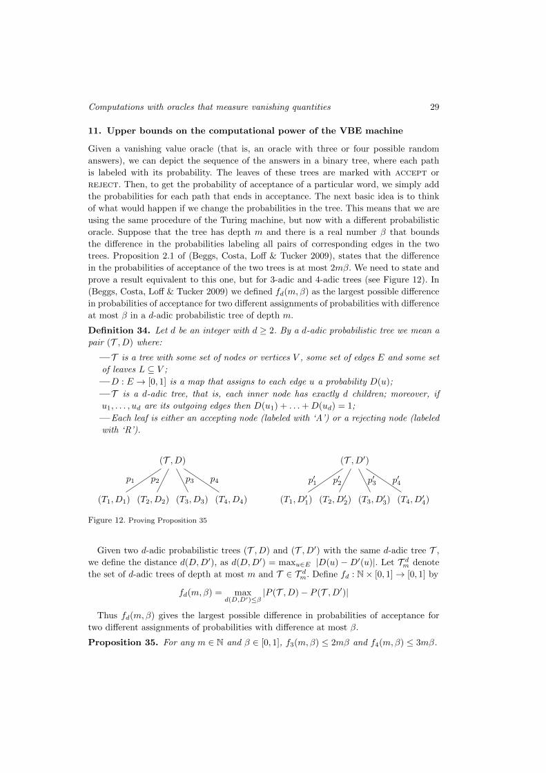
Computations with oracles that measure vanishing quantities 29
11. Upper bounds on the computational power of the VBE machine
Given a vanishing value oracle (that is, an oracle with three or four possible random
answers), we can depict the sequence of the answers in a binary tree, where each path
is labeled with its probability. The leaves of these trees are marked with accept or
reject. Then, to get the probability of acceptance of a particular word, we simply add
the probabilities for each path that ends in acceptance. The next basic idea is to think
of what would happen if we change the probabilities in the tree. This means that we are
using the same procedure of the Turing machine, but now with a different probabilistic
oracle. Suppose that the tree has depth m and there is a real number β that bounds
the difference in the probabilities labeling all pairs of corresponding edges in the two
trees. Proposition 2.1 of (Beggs, Costa, Loff & Tucker 2009), states that the difference
in the probabilities of acceptance of the two trees is at most 2mβ. We need to state and
prove a result equivalent to this one, but for 3-adic and 4-adic trees (see Figure 12). In
(Beggs, Costa, Loff & Tucker 2009) we defined fd(m,β) as the largest possible difference
in probabilities of acceptance for two different assignments of probabilities with difference
at most β in a d-adic probabilistic tree of depth m.
Definition 34. Let d be an integer with d ≥ 2. By a d-adic probabilistic tree we mean a
pair (T , D) where:
—T is a tree with some set of nodes or vertices V , some set of edges E and some set
of leaves L ⊆ V ;
—D : E → [0, 1] is a map that assigns to each edge u a probability D(u);
—T is a d-adic tree, that is, each inner node has exactly d children; moreover, if
u1, . . . , ud are its outgoing edges then D(u1) + . . .+D(ud) = 1;
—Each leaf is either an accepting node (labeled with ‘A’) or a rejecting node (labeled
with ‘R’).
(T , D)
(T1, D1)
p1
(T2, D2)
p2
(T3, D3)
p3
(T4, D4)
p4
(T , D′)
(T1, D′1)
p′1
(T2, D′2)
p′2
(T3, D′3)
p′3
(T4, D′4)
p′4
Figure 12. Proving Proposition 35
Given two d-adic probabilistic trees (T , D) and (T , D′) with the same d-adic tree T ,
we define the distance d(D,D′), as d(D,D′) = maxu∈E |D(u) −D′(u)|. Let T dm denote
the set of d-adic trees of depth at most m and T ∈ T dm. Define fd : N× [0, 1]→ [0, 1] by
fd(m,β) = maxd(D,D′)≤β
|P (T , D)− P (T , D′)|
Thus fd(m,β) gives the largest possible difference in probabilities of acceptance for
two different assignments of probabilities with difference at most β.
Proposition 35. For any m ∈ N and β ∈ [0, 1], f3(m,β) ≤ 2mβ and f4(m,β) ≤ 3mβ.
Edwin Beggs, Jose Felix Costa, Diogo Pocas & John V Tucker 30
Proof: This proposition is a generalization of Proposition 2.1 in (Beggs, Costa, Loff &
Tucker 2009). The proof involves some algebra but is more or less straightforward.
Proposition 36. If A is decidable in polynomial time by the VBE machine M(y) for
y ∈ (0, 1) operating with any protocol P with exponential time schedule, then A ∈ P/poly.
Proof: Let A be a set decidable by the VBE machine operating with protocol P with an
exponential schedule T . Let c and d be constants such that, for an input word of size
n, all queries have size at most dc log n + de. A query of size k is defined by two dyadic
rationals of size k, so there are exactly 22k possible queries of size k. This means that
the number of different possible queries in a computation with an input word of size n
is at most polynomial in n:
dc logn+de∑i=1
22i <22d+2
3n2c .
If P is deterministic, then the advice function f is the concatenation of all triples
〈z1, z2, r〉 such that z1 and z2 are dyadic rationals of size k ≤ dc log n+ de and r encodes
the result of protocol call Compare[P](z1, z2). (There are either three or four possible
results, so r may be encoded with only two bits.) If P is probabilistic, then the advice
function f is the concatenation of all tuples 〈z1, z2, pf , ps, pt, pu〉 such that z1 and
z2 are dyadic rationals of size k ≤ dc log n + de and pf , ps, pt, pu are approximations to
the probabilities of obtaining each possible result (“first”, “second”, “timeout” or
“undistinguishable”) of protocol call Compare[P](z1, z2). We will approximate each
probability with a dyadic rational of size k such that the error in the probability of any
query is bounded by 2−k. To find the suitable value of k, we observe that the VBE machine
deciding A runs in polynomial time O(na) and so the number of possible queries in the
computation of any word of size n is at most bna, for some constant b. The probabilistic
tree induced by the computation has a depth at most bna. Now, if γ is the bound on the
error probability associated with the machine, by Proposition 35, we take k such that
3bna2−k < 1/2 − γ, that is, 2k > 3bna/(1/2 − γ). Such a k can then be taken to be
logarithmic in n. In either case f ∈ poly since f is the concatenation of a polynomial
amount of tuples each with logarithmic size.
We specify a Turing machineM to decide A in polynomial time using f as advice.Msimulates the VBE machine for the same input word. When reaching a query state with
query words z1 and z2, it reads the appropriate tuple in f . In the deterministic case, the
machine resumes the computation in the proper outcome state. In the probabilistic case,
the machine uses the approximations to the probabilities of each result and choose one
of them with k coin tosses. In the deterministic case, it is clear that this machine decides
A in polynomial time. In the probabilistic case, this machine induces a probabilistic tree
in the same way as the original machine, with depth less than bna and edge difference
lower than 2−k. Then, by Proposition 35 and the above calculations, the difference in the
probabilities of acceptance is then bounded by a constant less than 1/2 − γ. Thus, the
probability that this machine gives a wrong answer is bounded by a constant less than
1/2, and so the machine specified decides A in polynomial time. This proposition is not enough for our purposes: in the first implementation we will be
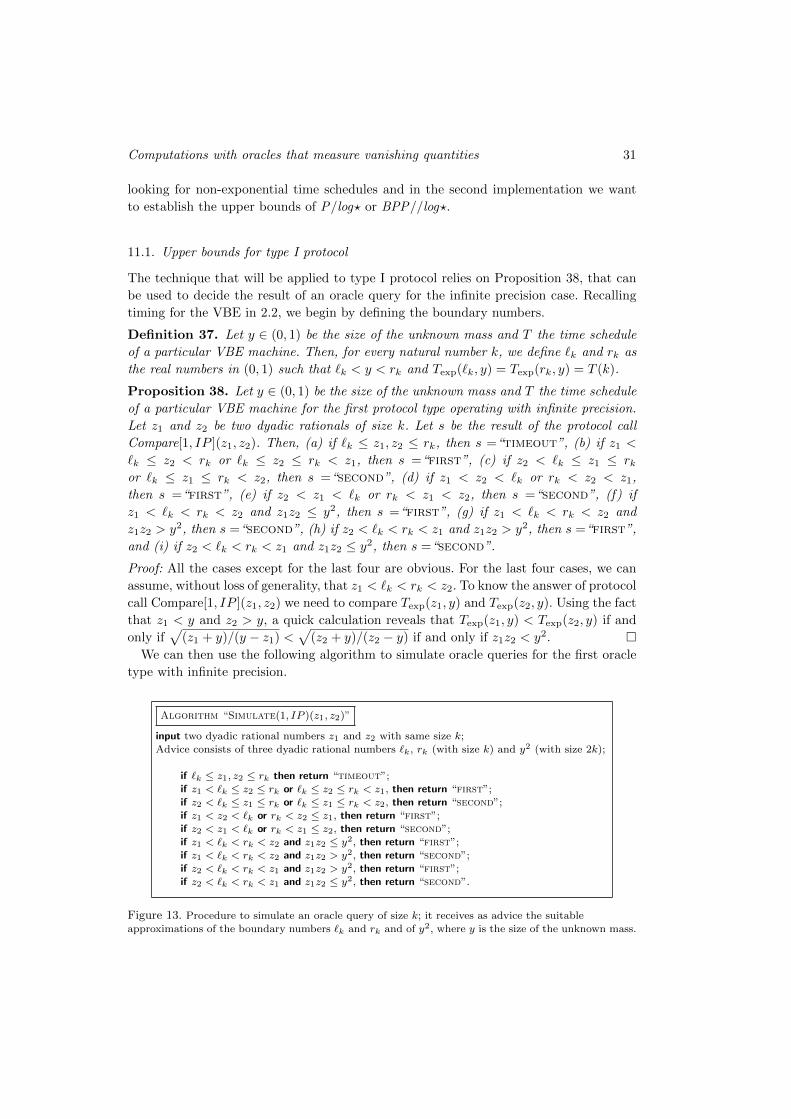
Computations with oracles that measure vanishing quantities 31
looking for non-exponential time schedules and in the second implementation we want
to establish the upper bounds of P/log? or BPP//log?.
11.1. Upper bounds for type I protocol
The technique that will be applied to type I protocol relies on Proposition 38, that can
be used to decide the result of an oracle query for the infinite precision case. Recalling
timing for the VBE in 2.2, we begin by defining the boundary numbers.
Definition 37. Let y ∈ (0, 1) be the size of the unknown mass and T the time schedule
of a particular VBE machine. Then, for every natural number k, we define `k and rk as
the real numbers in (0, 1) such that `k < y < rk and Texp(`k, y) = Texp(rk, y) = T (k).
Proposition 38. Let y ∈ (0, 1) be the size of the unknown mass and T the time schedule
of a particular VBE machine for the first protocol type operating with infinite precision.
Let z1 and z2 be two dyadic rationals of size k. Let s be the result of the protocol call
Compare[1, IP ](z1, z2). Then, (a) if `k ≤ z1, z2 ≤ rk, then s =“timeout”, (b) if z1 <
`k ≤ z2 < rk or `k ≤ z2 ≤ rk < z1, then s =“first”, (c) if z2 < `k ≤ z1 ≤ rkor `k ≤ z1 ≤ rk < z2, then s =“second”, (d) if z1 < z2 < `k or rk < z2 < z1,
then s =“first”, (e) if z2 < z1 < `k or rk < z1 < z2, then s =“second”, (f) if
z1 < `k < rk < z2 and z1z2 ≤ y2, then s =“first”, (g) if z1 < `k < rk < z2 and
z1z2 > y2, then s =“second”, (h) if z2 < `k < rk < z1 and z1z2 > y2, then s =“first”,
and (i) if z2 < `k < rk < z1 and z1z2 ≤ y2, then s =“second”.
Proof: All the cases except for the last four are obvious. For the last four cases, we can
assume, without loss of generality, that z1 < `k < rk < z2. To know the answer of protocol
call Compare[1, IP ](z1, z2) we need to compare Texp(z1, y) and Texp(z2, y). Using the fact
that z1 < y and z2 > y, a quick calculation reveals that Texp(z1, y) < Texp(z2, y) if and
only if√
(z1 + y)/(y − z1) <√
(z2 + y)/(z2 − y) if and only if z1z2 < y2. We can then use the following algorithm to simulate oracle queries for the first oracle
type with infinite precision.
Algorithm “Simulate(1, IP )(z1, z2)”
input two dyadic rational numbers z1 and z2 with same size k;
Advice consists of three dyadic rational numbers `k, rk (with size k) and y2 (with size 2k);
if `k ≤ z1, z2 ≤ rk then return “timeout”;
if z1 < `k ≤ z2 ≤ rk or `k ≤ z2 ≤ rk < z1, then return “first”;
if z2 < `k ≤ z1 ≤ rk or `k ≤ z1 ≤ rk < z2, then return “second”;if z1 < z2 < `k or rk < z2 ≤ z1, then return “first”;
if z2 < z1 < `k or rk < z1 ≤ z2, then return “second”;
if z1 < `k < rk < z2 and z1z2 ≤ y2, then return “first”;if z1 < `k < rk < z2 and z1z2 > y2, then return “second”;
if z2 < `k < rk < z1 and z1z2 > y2, then return “first”;
if z2 < `k < rk < z1 and z1z2 ≤ y2, then return “second”.
Figure 13. Procedure to simulate an oracle query of size k; it receives as advice the suitable
approximations of the boundary numbers `k and rk and of y2, where y is the size of the unknown mass.
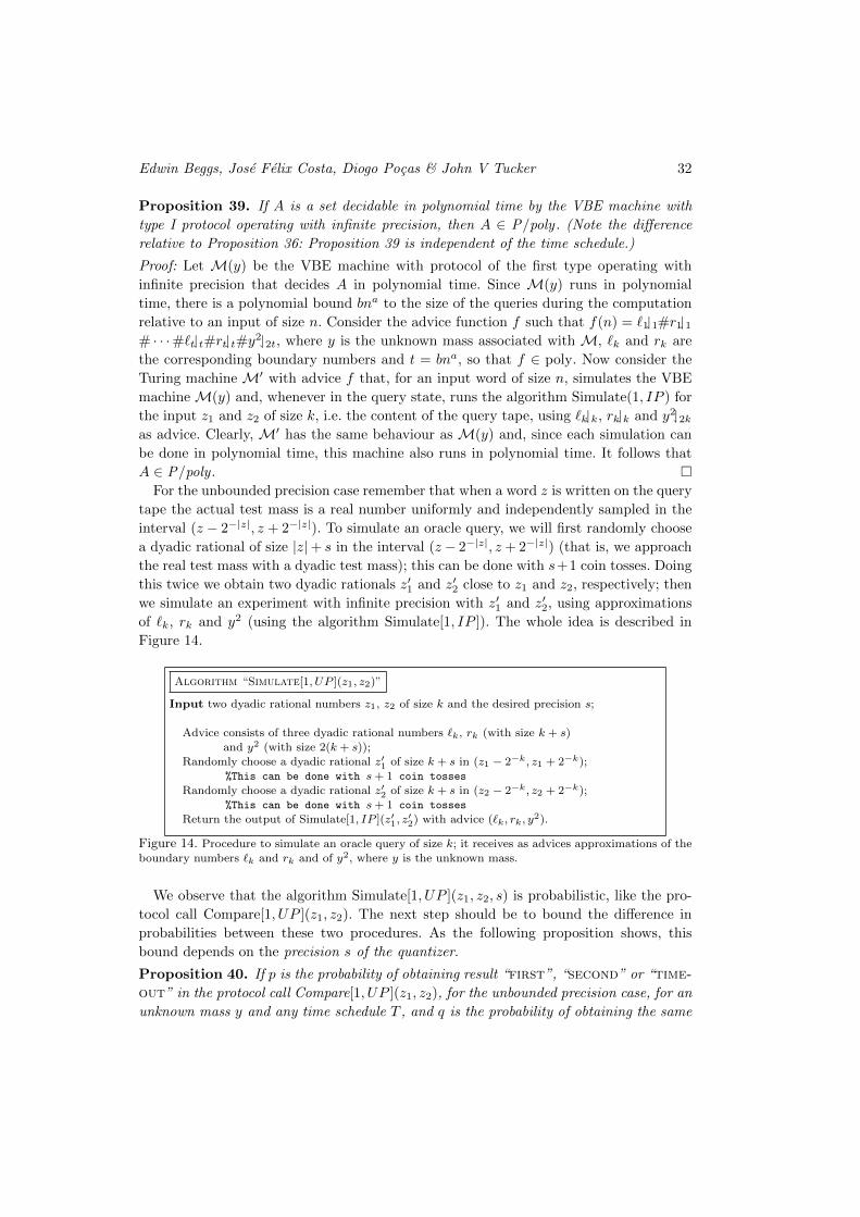
Edwin Beggs, Jose Felix Costa, Diogo Pocas & John V Tucker 32
Proposition 39. If A is a set decidable in polynomial time by the VBE machine with
type I protocol operating with infinite precision, then A ∈ P/poly. (Note the difference
relative to Proposition 36: Proposition 39 is independent of the time schedule.)
Proof: Let M(y) be the VBE machine with protocol of the first type operating with
infinite precision that decides A in polynomial time. Since M(y) runs in polynomial
time, there is a polynomial bound bna to the size of the queries during the computation
relative to an input of size n. Consider the advice function f such that f(n) = `11#r11# · · ·#`tt#rtt#y22t, where y is the unknown mass associated with M, `k and rk are
the corresponding boundary numbers and t = bna, so that f ∈ poly. Now consider the
Turing machine M′ with advice f that, for an input word of size n, simulates the VBE
machineM(y) and, whenever in the query state, runs the algorithm Simulate(1, IP ) for
the input z1 and z2 of size k, i.e. the content of the query tape, using `kk, rkk and y22kas advice. Clearly, M′ has the same behaviour as M(y) and, since each simulation can
be done in polynomial time, this machine also runs in polynomial time. It follows that
A ∈ P/poly . For the unbounded precision case remember that when a word z is written on the query
tape the actual test mass is a real number uniformly and independently sampled in the
interval (z − 2−|z|, z + 2−|z|). To simulate an oracle query, we will first randomly choose
a dyadic rational of size |z|+ s in the interval (z − 2−|z|, z + 2−|z|) (that is, we approach
the real test mass with a dyadic test mass); this can be done with s+1 coin tosses. Doing
this twice we obtain two dyadic rationals z′1 and z′2 close to z1 and z2, respectively; then
we simulate an experiment with infinite precision with z′1 and z′2, using approximations
of `k, rk and y2 (using the algorithm Simulate[1, IP ]). The whole idea is described in
Figure 14.
Algorithm “Simulate[1, UP ](z1, z2)”
Input two dyadic rational numbers z1, z2 of size k and the desired precision s;
Advice consists of three dyadic rational numbers `k, rk (with size k + s)and y2 (with size 2(k + s));
Randomly choose a dyadic rational z′1 of size k + s in (z1 − 2−k, z1 + 2−k);
%This can be done with s+ 1 coin tosses
Randomly choose a dyadic rational z′2 of size k + s in (z2 − 2−k, z2 + 2−k);
%This can be done with s+ 1 coin tosses
Return the output of Simulate[1, IP ](z′1, z′2) with advice (`k, rk, y
2).
Figure 14. Procedure to simulate an oracle query of size k; it receives as advices approximations of the
boundary numbers `k and rk and of y2, where y is the unknown mass.
We observe that the algorithm Simulate[1, UP ](z1, z2, s) is probabilistic, like the pro-
tocol call Compare[1, UP ](z1, z2). The next step should be to bound the difference in
probabilities between these two procedures. As the following proposition shows, this
bound depends on the precision s of the quantizer.
Proposition 40. If p is the probability of obtaining result “first”, “second” or “time-
out” in the protocol call Compare[1, UP ](z1, z2), for the unbounded precision case, for an
unknown mass y and any time schedule T , and q is the probability of obtaining the same
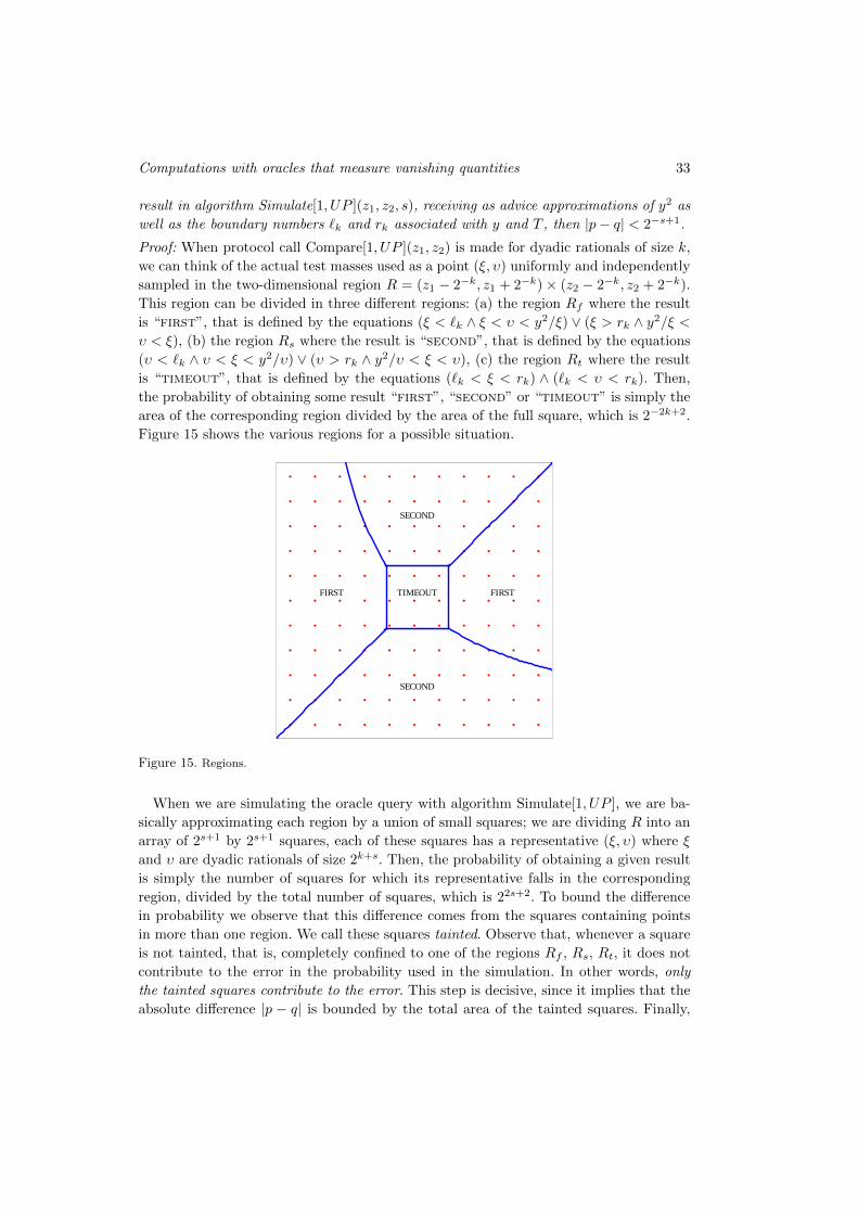
Computations with oracles that measure vanishing quantities 33
result in algorithm Simulate[1, UP ](z1, z2, s), receiving as advice approximations of y2 as
well as the boundary numbers `k and rk associated with y and T , then |p− q| < 2−s+1.
Proof: When protocol call Compare[1, UP ](z1, z2) is made for dyadic rationals of size k,
we can think of the actual test masses used as a point (ξ, υ) uniformly and independently
sampled in the two-dimensional region R = (z1 − 2−k, z1 + 2−k)× (z2 − 2−k, z2 + 2−k).
This region can be divided in three different regions: (a) the region Rf where the result
is “first”, that is defined by the equations (ξ < `k ∧ ξ < υ < y2/ξ) ∨ (ξ > rk ∧ y2/ξ <υ < ξ), (b) the region Rs where the result is “second”, that is defined by the equations
(υ < `k ∧ υ < ξ < y2/υ) ∨ (υ > rk ∧ y2/υ < ξ < υ), (c) the region Rt where the result
is “timeout”, that is defined by the equations (`k < ξ < rk) ∧ (`k < υ < rk). Then,
the probability of obtaining some result “first”, “second” or “timeout” is simply the
area of the corresponding region divided by the area of the full square, which is 2−2k+2.
Figure 15 shows the various regions for a possible situation.
TIMEOUTFIRST FIRST
SECOND
SECOND
Figure 15. Regions.
When we are simulating the oracle query with algorithm Simulate[1, UP ], we are ba-
sically approximating each region by a union of small squares; we are dividing R into an
array of 2s+1 by 2s+1 squares, each of these squares has a representative (ξ, υ) where ξ
and υ are dyadic rationals of size 2k+s. Then, the probability of obtaining a given result
is simply the number of squares for which its representative falls in the corresponding
region, divided by the total number of squares, which is 22s+2. To bound the difference
in probability we observe that this difference comes from the squares containing points
in more than one region. We call these squares tainted. Observe that, whenever a square
is not tainted, that is, completely confined to one of the regions Rf , Rs, Rt, it does not
contribute to the error in the probability used in the simulation. In other words, only
the tainted squares contribute to the error. This step is decisive, since it implies that the
absolute difference |p − q| is bounded by the total area of the tainted squares. Finally,
Edwin Beggs, Jose Felix Costa, Diogo Pocas & John V Tucker 34
a simple counting argument reveals that the total number of tainted squares is at most
2(2× 2s+1 − 1)− 1 < 2s+3. In this way, we obtain the desired bound in the difference of
probabilities, as |p− q| < 2s+3/22s+2 = 2−s+1.
Proposition 41. If A is a set decidable in polynomial time by the VBE machine oper-
ating with type I protocol and unbounded precision, then A ∈ P/poly.¶
Proof: Let A be decidable in polynomial time by the VBE machine operating with type
I protocol and unbounded precision. We will prove that A ∈ BPP//poly . There is a
polynomial bound bna on both the size of a query and the number of queries that can
be made during the computation on an input word of size n. We want to approximate
the probability of any possible result of any possible query with a dyadic rational of size
e, for a suitable e, such that the difference in probabilities of any query is bounded by
2−e. If γ is the bound on the error probability associated with the VBE machine, then,
by Proposition 35, the suitable value of e must be such that 2× bna2−e < 1/2− γ, that
is, 2e > 2bna/(1/2− γ). (The probabilistic tree induced by the VBE machine is ternary
in this case.) Such a e can be taken to be logarithmic in n.
Now we consider the advice function f such that f(n) = `12+e #r12+e # · · ·#`tt+e+1#rtt+e+1#y22(t+e+1), where y is the unknown mass associated with the VBE
machine, `k and rk are the corresponding boundary numbers and t = bna. It is immediate
that f ∈ poly. We specify a machine for deciding the set A in polynomial time, using f as
advice. This machine simulates the VBE machine for the same input word. Whenever in
a query state with query words z1 and z2 of size k, it runs algorithm Simulate(1, UP ) for
the input z1, z2 (in the query tape) and e+1, using `kk+e+1, rkk+e+1 and y22(k+e+1) as
advice. This machine induces a probabilistic tree in the same way as the original machine,
with depth lower than bna. Thanks to Proposition 40, the edge difference is also lower
than 2−e. Then, by Proposition 35, the difference in the probabilities of acceptance is
bounded by a constant less than 1/2−γ. Since each simulation can be done in polynomial
time, this machine also runs in polynomial time. It follows that A ∈ BPP//poly =P/poly .
The remaining case is that of the fixed precision ε. The idea is the same as in the
unbounded precision case, that is, we will devise a randomized algorithm to simulate
oracle queries. For two given dyadic rationals z1, z2 we discretize the region R = (z1 −ε, z1 + ε)× (z2− ε, z2 + ε). In the unbounded precision case it was easy to select a dyadic
rational of fixed size in the interval (z − 2−|z|, z + 2−|z|) since the amplitude was itself
a dyadic rational; for the fixed precision we have to deal with the fact that ε may not
be a dyadic rational. The idea that we will use is as follows: let t be a natural number
such that 2−t−1 < ε ≤ 2−t; we randomly choose a dyadic rational z′ ∈ (z − 2−t, z + 2−t)
of size σ (this can be done with σ − t + 1 coin tosses);‖ then with probability at least
1/2 we obtain that z′ ∈ (z − ε, z + ε). If we repeat the above procedure h times then we
¶ Again, this result does not depend on any particular time schedule.‖ Observe that σ may be smaller than |z|; i.e. the dyadic rational generated has smaller size than z;
the intuitive meaning of this is that increasing the size of the queries does not contribute to increasetheir precision.
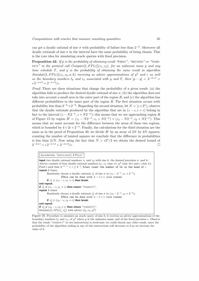
Computations with oracles that measure vanishing quantities 35
can get a dyadic rational of size σ with probability of failure less than 2−h. Moreover all
dyadic rationals of size σ in the interval have the same probability of being chosen. This
is the core idea for simulating oracle queries with fixed precision.
Proposition 42. If p is the probability of obtaining result “first”, “second” or “time-
out” in the protocol call Compare[1, FP (ε)](z1, z2), for an unknown mass y and any
time schedule T , and q is the probability of obtaining the same result in algorithm
Simulate[1, FP (ε)](z1, z2, σ, h) receiving as advice approximations of y2 and ε as well
as the boundary numbers `k and rk associated with y and T , then |p − q| < 2−h+1 +
ε 2−σ+3 + 2−σ+2/ε.
Proof: There are three situations that change the probability of a given result: (a) the
algorithm fails to produce the desired dyadic rational of size σ, (b) the algorithm does not
take into account a small area in the outer part of the region R, and (c) the algorithm has
different probabilities in the inner part of the region R. The first situation occurs with
probability less than 2−h+2−h. Regarding the second situation, let N = bε×2σc; observe
that the dyadic rationals produced by the algorithm that are in (z − ε, z + ε) belong in
fact to the interval (z −N2−σ, z +N2−σ); this means that we are approaching region R
of Figure 15 by region R′ = (z1 − N2−σ, z1 + N2−σ) × (z2 − N2−σ, z2 + N2−σ). This
means that we must account for the difference between the areas of these two regions,
which is bounded by 4×2ε×2−σ. Finally, the calculations for the third situation are the
same as in the proof of Proposition 40; we divide R′ by an array of 2N by 2N squares;
counting the number of tainted squares we conclude that the difference in probabilities
is less than 2/N . Now using the fact that N > ε2σ/2 we obtain the desired bound of
2−h+1 + ε 2−σ+3 + 2−σ+2/ε.
Algorithm “simulate(1, FP (ε))”
input two dyadic rational numbers z1 and z2 with size k, the desired precision σ, and h;
Advice consists of four dyadic rational numbers `k, rk (size σ), y2 (size 2σ) and ε (size σ);Find t such that 2−t−1 < ε ≤ 2−t; %Just count the number of 0s in the head of ε
repeat h times
Randomly choose a dyadic rational z′1 of size σ in (z1 − 2−t, z1 + 2−t);%This can be done with σ − t+ 1 coin tosses
if z′1 ∈ (z1 − ε, z1 + ε) then break;
end repeat;if z′1 6∈ (z1 − ε, z1 + ε) then return “timeout”;
repeat h times
Randomly choose a dyadic rational z′2 of size σ in (z2 − 2−t, z2 + 2−t);%This can be done with σ − t+ 1 coin tosses
if z′2 ∈ (z2 − ε, z2 + ε) then break;
end repeat;if z′2 6∈ (z2 − ε, z2 + ε) then return “timeout”;
Simulate[1, IP ](z′1, z′2) with advice (`k, rk, y
2)
Figure 16. Procedure to simulate an oracle query of size k; it receives as advice approximations of the
boundary numbers `k and rk, of y2 where y is the unknown mass, and of the fixed precision ε. Observe
that the result “timeout” in two instructions is irrelevant; we could choose any other result, since theprobability of the algorithm ending in any of this instructions will decrease to 0 as we increase the
value of h.
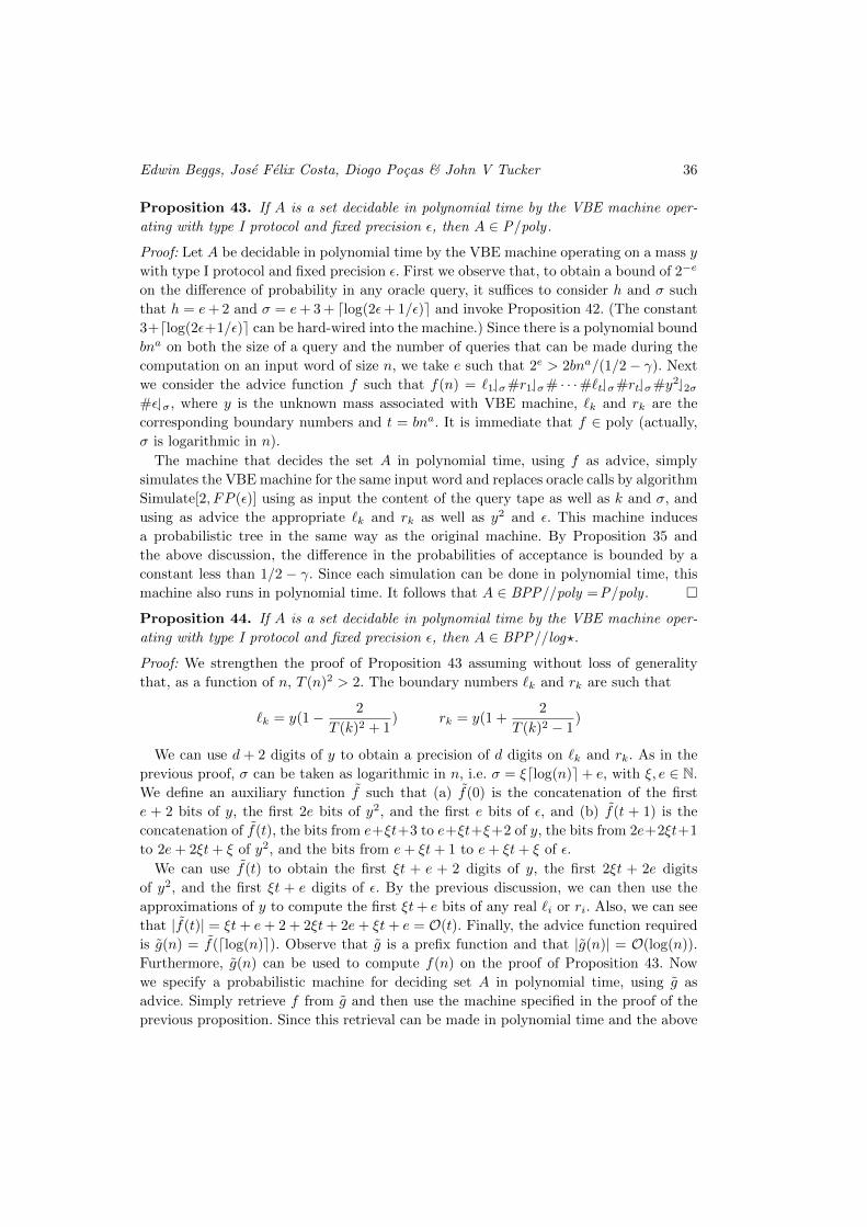
Edwin Beggs, Jose Felix Costa, Diogo Pocas & John V Tucker 36
Proposition 43. If A is a set decidable in polynomial time by the VBE machine oper-
ating with type I protocol and fixed precision ε, then A ∈ P/poly.
Proof: Let A be decidable in polynomial time by the VBE machine operating on a mass y
with type I protocol and fixed precision ε. First we observe that, to obtain a bound of 2−e
on the difference of probability in any oracle query, it suffices to consider h and σ such
that h = e+ 2 and σ = e+ 3 + dlog(2ε+ 1/ε)e and invoke Proposition 42. (The constant
3+dlog(2ε+1/ε)e can be hard-wired into the machine.) Since there is a polynomial bound
bna on both the size of a query and the number of queries that can be made during the
computation on an input word of size n, we take e such that 2e > 2bna/(1/2− γ). Next
we consider the advice function f such that f(n) = `1σ#r1σ# · · ·#`tσ#rtσ#y22σ#εσ, where y is the unknown mass associated with VBE machine, `k and rk are the
corresponding boundary numbers and t = bna. It is immediate that f ∈ poly (actually,
σ is logarithmic in n).
The machine that decides the set A in polynomial time, using f as advice, simply
simulates the VBE machine for the same input word and replaces oracle calls by algorithm
Simulate[2, FP (ε)] using as input the content of the query tape as well as k and σ, and
using as advice the appropriate `k and rk as well as y2 and ε. This machine induces
a probabilistic tree in the same way as the original machine. By Proposition 35 and
the above discussion, the difference in the probabilities of acceptance is bounded by a
constant less than 1/2 − γ. Since each simulation can be done in polynomial time, this
machine also runs in polynomial time. It follows that A ∈ BPP//poly =P/poly .
Proposition 44. If A is a set decidable in polynomial time by the VBE machine oper-
ating with type I protocol and fixed precision ε, then A ∈ BPP//log?.
Proof: We strengthen the proof of Proposition 43 assuming without loss of generality
that, as a function of n, T (n)2 > 2. The boundary numbers `k and rk are such that
`k = y(1− 2
T (k)2 + 1) rk = y(1 +
2
T (k)2 − 1)
We can use d + 2 digits of y to obtain a precision of d digits on `k and rk. As in the
previous proof, σ can be taken as logarithmic in n, i.e. σ = ξdlog(n)e+ e, with ξ, e ∈ N.
We define an auxiliary function f such that (a) f(0) is the concatenation of the first
e + 2 bits of y, the first 2e bits of y2, and the first e bits of ε, and (b) f(t + 1) is the
concatenation of f(t), the bits from e+ξt+3 to e+ξt+ξ+2 of y, the bits from 2e+2ξt+1
to 2e+ 2ξt+ ξ of y2, and the bits from e+ ξt+ 1 to e+ ξt+ ξ of ε.
We can use f(t) to obtain the first ξt + e + 2 digits of y, the first 2ξt + 2e digits
of y2, and the first ξt + e digits of ε. By the previous discussion, we can then use the
approximations of y to compute the first ξt+ e bits of any real `i or ri. Also, we can see
that |f(t)| = ξt+ e+ 2 + 2ξt+ 2e+ ξt+ e = O(t). Finally, the advice function required
is g(n) = f(dlog(n)e). Observe that g is a prefix function and that |g(n)| = O(log(n)).
Furthermore, g(n) can be used to compute f(n) on the proof of Proposition 43. Now
we specify a probabilistic machine for deciding set A in polynomial time, using g as
advice. Simply retrieve f from g and then use the machine specified in the proof of the
previous proposition. Since this retrieval can be made in polynomial time and the above
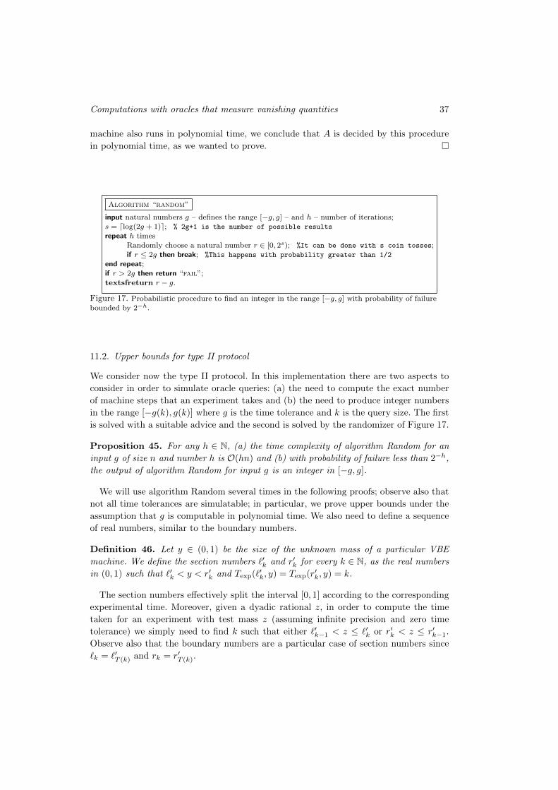
Computations with oracles that measure vanishing quantities 37
machine also runs in polynomial time, we conclude that A is decided by this procedure
in polynomial time, as we wanted to prove.
Algorithm “random”
input natural numbers g – defines the range [−g, g] – and h – number of iterations;
s = dlog(2g + 1)e; % 2g+1 is the number of possible results
repeat h times
Randomly choose a natural number r ∈ [0, 2s); %It can be done with s coin tosses;
if r ≤ 2g then break; %This happens with probability greater than 1/2
end repeat;if r > 2g then return “fail”;
textsfreturn r − g.
Figure 17. Probabilistic procedure to find an integer in the range [−g, g] with probability of failure
bounded by 2−h.
11.2. Upper bounds for type II protocol
We consider now the type II protocol. In this implementation there are two aspects to
consider in order to simulate oracle queries: (a) the need to compute the exact number
of machine steps that an experiment takes and (b) the need to produce integer numbers
in the range [−g(k), g(k)] where g is the time tolerance and k is the query size. The first
is solved with a suitable advice and the second is solved by the randomizer of Figure 17.
Proposition 45. For any h ∈ N, (a) the time complexity of algorithm Random for an
input g of size n and number h is O(hn) and (b) with probability of failure less than 2−h,
the output of algorithm Random for input g is an integer in [−g, g].
We will use algorithm Random several times in the following proofs; observe also that
not all time tolerances are simulatable; in particular, we prove upper bounds under the
assumption that g is computable in polynomial time. We also need to define a sequence
of real numbers, similar to the boundary numbers.
Definition 46. Let y ∈ (0, 1) be the size of the unknown mass of a particular VBE
machine. We define the section numbers `′k and r′k for every k ∈ N, as the real numbers
in (0, 1) such that `′k < y < r′k and Texp(`′k, y) = Texp(r′k, y) = k.
The section numbers effectively split the interval [0, 1] according to the corresponding
experimental time. Moreover, given a dyadic rational z, in order to compute the time
taken for an experiment with test mass z (assuming infinite precision and zero time
tolerance) we simply need to find k such that either `′k−1 < z ≤ `′k or r′k < z ≤ r′k−1.
Observe also that the boundary numbers are a particular case of section numbers since
`k = `′T (k) and rk = r′T (k).
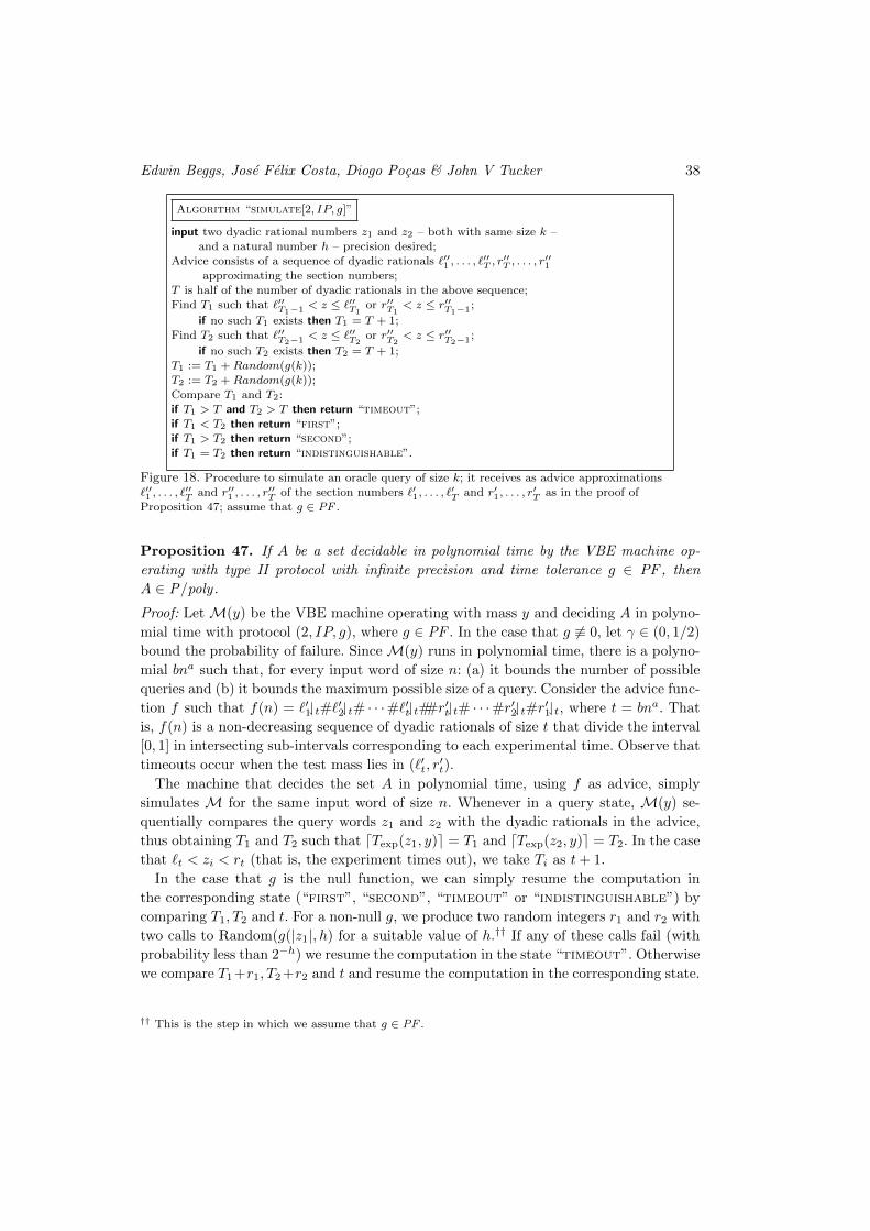
Edwin Beggs, Jose Felix Costa, Diogo Pocas & John V Tucker 38
Algorithm “simulate[2, IP, g]”
input two dyadic rational numbers z1 and z2 – both with same size k –
and a natural number h – precision desired;Advice consists of a sequence of dyadic rationals `′′1 , . . . , `
′′T , r′′T , . . . , r
′′1
approximating the section numbers;
T is half of the number of dyadic rationals in the above sequence;Find T1 such that `′′T1−1 < z ≤ `′′T1
or r′′T1< z ≤ r′′T1−1;
if no such T1 exists then T1 = T + 1;
Find T2 such that `′′T2−1 < z ≤ `′′T2or r′′T2
< z ≤ r′′T2−1;
if no such T2 exists then T2 = T + 1;
T1 := T1 +Random(g(k));
T2 := T2 +Random(g(k));Compare T1 and T2:
if T1 > T and T2 > T then return “timeout”;if T1 < T2 then return “first”;
if T1 > T2 then return “second”;
if T1 = T2 then return “indistinguishable”.
Figure 18. Procedure to simulate an oracle query of size k; it receives as advice approximations
`′′1 , . . . , `′′T and r′′1 , . . . , r
′′T of the section numbers `′1, . . . , `
′T and r′1, . . . , r
′T as in the proof of
Proposition 47; assume that g ∈ PF .
Proposition 47. If A be a set decidable in polynomial time by the VBE machine op-
erating with type II protocol with infinite precision and time tolerance g ∈ PF , then
A ∈ P/poly.
Proof: Let M(y) be the VBE machine operating with mass y and deciding A in polyno-
mial time with protocol (2, IP, g), where g ∈ PF . In the case that g 6≡ 0, let γ ∈ (0, 1/2)
bound the probability of failure. SinceM(y) runs in polynomial time, there is a polyno-
mial bna such that, for every input word of size n: (a) it bounds the number of possible
queries and (b) it bounds the maximum possible size of a query. Consider the advice func-
tion f such that f(n) = `′1t#`′2t# · · ·#`′tt##r′tt# · · ·#r′2t#r′1t, where t = bna. That
is, f(n) is a non-decreasing sequence of dyadic rationals of size t that divide the interval
[0, 1] in intersecting sub-intervals corresponding to each experimental time. Observe that
timeouts occur when the test mass lies in (`′t, r′t).
The machine that decides the set A in polynomial time, using f as advice, simply
simulates M for the same input word of size n. Whenever in a query state, M(y) se-
quentially compares the query words z1 and z2 with the dyadic rationals in the advice,
thus obtaining T1 and T2 such that dTexp(z1, y)e = T1 and dTexp(z2, y)e = T2. In the case
that `t < zi < rt (that is, the experiment times out), we take Ti as t+ 1.
In the case that g is the null function, we can simply resume the computation in
the corresponding state (“first”, “second”, “timeout” or “indistinguishable”) by
comparing T1, T2 and t. For a non-null g, we produce two random integers r1 and r2 with
two calls to Random(g(|z1|, h) for a suitable value of h.†† If any of these calls fail (with
probability less than 2−h) we resume the computation in the state “timeout”. Otherwise
we compare T1+r1, T2+r2 and t and resume the computation in the corresponding state.
†† This is the step in which we assume that g ∈ PF .
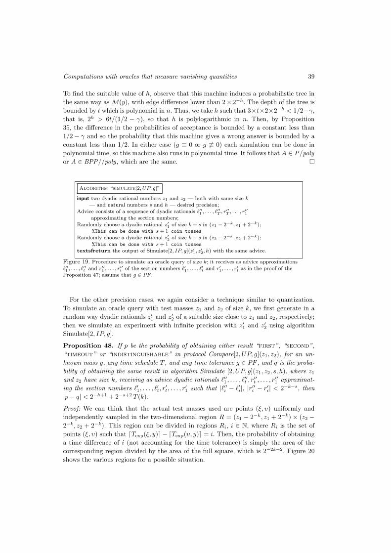
Computations with oracles that measure vanishing quantities 39
To find the suitable value of h, observe that this machine induces a probabilistic tree in
the same way asM(y), with edge difference lower than 2× 2−h. The depth of the tree is
bounded by t which is polynomial in n. Thus, we take h such that 3×t×2×2−h < 1/2−γ,
that is, 2h > 6t/(1/2 − γ), so that h is polylogarithmic in n. Then, by Proposition
35, the difference in the probabilities of acceptance is bounded by a constant less than
1/2− γ and so the probability that this machine gives a wrong answer is bounded by a
constant less than 1/2. In either case (g ≡ 0 or g 6≡ 0) each simulation can be done in
polynomial time, so this machine also runs in polynomial time. It follows that A ∈ P/poly
or A ∈ BPP//poly , which are the same.
Algorithm “simulate[2, UP, g]”
input two dyadic rational numbers z1 and z2 — both with same size k
— and natural numbers s and h — desired precision;Advice consists of a sequence of dyadic rationals `′′1 , . . . , `
′′T , r′′T , . . . , r
′′1
approximating the section numbers;
Randomly choose a dyadic rational z′1 of size k + s in (z1 − 2−k, z1 + 2−k);%This can be done with s+ 1 coin tosses
Randomly choose a dyadic rational z′2 of size k + s in (z2 − 2−k, z2 + 2−k);
%This can be done with s+ 1 coin tosses
textsfreturn the output of Simulate[2, IP, g](z′1, z′2, h) with the same advice.
Figure 19. Procedure to simulate an oracle query of size k; it receives as advice approximations`′′1 , . . . , `
′′t and r′′1 , . . . , r
′′t of the section numbers `′1, . . . , `
′t and r′1, . . . , r
′t as in the proof of the
Proposition 47; assume that g ∈ PF .
For the other precision cases, we again consider a technique similar to quantization.
To simulate an oracle query with test masses z1 and z2 of size k, we first generate in a
random way dyadic rationals z′1 and z′2 of a suitable size close to z1 and z2, respectively;
then we simulate an experiment with infinite precision with z′1 and z′2 using algorithm
Simulate[2, IP, g].
Proposition 48. If p be the probability of obtaining either result “first”, “second”,
“timeout” or “indistinguishable” in protocol Compare[2, UP, g](z1, z2), for an un-
known mass y, any time schedule T , and any time tolerance g ∈ PF , and q is the proba-
bility of obtaining the same result in algorithm Simulate [2, UP, g](z1, z2, s, h), where z1and z2 have size k, receiving as advice dyadic rationals `′′1 , . . . , `
′′t , r′′t , . . . , r
′′1 approximat-
ing the section numbers `′1, . . . , `′t, r′t, . . . , r
′1 such that |`′′i − `′i|, |r′′i − r′i| < 2−k−s, then
|p− q| < 2−h+1 + 2−s+2 T (k).
Proof: We can think that the actual test masses used are points (ξ, υ) uniformly and
independently sampled in the two-dimensional region R = (z1 − 2−k, z1 + 2−k) × (z2 −2−k, z2 + 2−k). This region can be divided in regions Ri, i ∈ N, where Ri is the set of
points (ξ, υ) such that dTexp(ξ, y)e − dTexp(υ, y)e = i. Then, the probability of obtaining
a time difference of i (not accounting for the time tolerance) is simply the area of the
corresponding region divided by the area of the full square, which is 2−2k+2. Figure 20
shows the various regions for a possible situation.
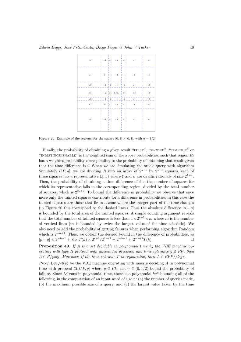
Edwin Beggs, Jose Felix Costa, Diogo Pocas & John V Tucker 40
T . O .
0
+ 1
+ 2
+ 3
+ 2
+ 1
0
- 1
0
+ 1
+ 2
+ 1
0
- 1
- 2
- 1
0
+ 1
0
- 1
- 2
- 3
- 2
- 1
- 1
- 2
- 3
- 2
- 1
0
+ 1
0
- 1
- 2
- 1
0
+ 1
+ 2
+ 1
0
- 1
0
+ 1
+ 2
+ 3
+ 2
+ 1
0
Figure 20. Example of the regions, for the square [0, 1]× [0, 1], with y = 1/2.
Finally, the probability of obtaining a given result “first”, “second”, “timeout” or
“indistinguishable” is the weighted sum of the above probabilities, such that region Rihas a weighted probability corresponding to the probability of obtaining that result given
that the time difference is i. When we are simulating the oracle query with algorithm
Simulate[2, UP, g], we are dividing R into an array of 2s+1 by 2s+1 squares, each of
these squares has a representative (ξ, υ) where ξ and υ are dyadic rationals of size 2k+s.
Then, the probability of obtaining a time difference of i is the number of squares for
which its representative falls in the corresponding region, divided by the total number
of squares, which is 22s+2. To bound the difference in probability we observe that once
more only the tainted squares contribute for a difference in probabilities; in this case the
tainted squares are those that lie in a zone where the integer part of the time changes
(in Figure 20 this correspond to the dashed lines). Thus the absolute difference |p − q|is bounded by the total area of the tainted squares. A simple counting argument reveals
that the total number of tainted squares is less than 4×2s+1×m where m is the number
of vertical lines (m is bounded by twice the largest value of the time schedule). We
also need to add the probability of getting failures when performing algorithm Random
which is 2−h+1. Thus, we obtain the desired bound in the difference of probabilities, as
|p− q| < 2−h+1 + 8× T (k)× 2s+1/22s+2 = 2−h+1 + 2−s+2T (k).
Proposition 49. If A is a set decidable in polynomial time by the VBE machine op-
erating with type II protocol with unbounded precision and time tolerance g ∈ PF , then
A ∈ P/poly. Moreover, if the time schedule T is exponential, then A ∈ BPP//log?.
Proof: Let M(y) be the VBE machine operating with mass y deciding A in polynomial
time with protocol (2, UP, g) where g ∈ PF . Let γ ∈ (0, 1/2) bound the probability of
failure. Since M runs in polynomial time, there is a polynomial bna bounding all of the
following, in the computation of an input word of size n: (a) the number of queries made,
(b) the maximum possible size of a query, and (c) the largest value taken by the time
Computations with oracles that measure vanishing quantities 41
schedule (that is, T (k) where k is the maximum possible size of a query). Consider the
advice function f such that f(n) = `′1t#`′2t# · · ·#`′tt##r′tt# · · ·#r′2t#r′1t, where
t = bna and t+ s for a suitable choice of s. That is, f(n) is a non-decreasing sequence of
dyadic rationals of size t+ s dividing the interval [0, 1] in sub-intervals corresponding to
each experimental time. Observe that timeouts occur when the test mass lies in (`′t, r′t).
The machine which decides set A in polynomial time, using the function f as advice,
simply simulatesM(y) for the same input word of size n and replaces protocol calls with
Simulate(2, UP, g)(z1, z2, s, h) for a suitable choice of h. The difference in probabilities,
by Proposition 48, is less than 2−h+1 + 2−s+2 t. To find the suitable values of s and
h, observe that this machine induces a probabilistic tree in the same way as M(y),
with depth bounded by t which is polynomial in n. Thus, we take h and s such that
3 × t × (2−h+1 + 2−s+2 t) < 1/2 − γ, for example, taking 2h > 12t/(1/2 − γ) and 2s >
24t2/(1/2 − γ), so that h and s are logarithmic in n. Then, by Proposition 35, the
difference in the probabilities of acceptance is bounded by a constant less than 1/2 − γand so the probability that this machine gives a wrong answer is bounded by a constant
less than 1/2. Since each simulation can be done in polynomial time, this machine also
runs in polynomial time. It follows that A ∈ P/poly .
Finally, in the assumption that T is exponential, the maximum possible size of a query
is bounded by some value σ which is logarithmic in n. But in this case we can take an
advice function f consisting on the binary expansion of y from which we can retrieve
approximations of `′i and r′i by taking `′′i = y (i2−1)/(i2 +1) and r′′i = y (i2 +1)/(i2−1).
It can be seen in a similar reasoning to previous proofs that to get an approximation
with precision 2−σ−s we need σ + s + 2 digits of y, thus f can be taken to be a prefix
function in log. Now we can retrieve f from f and repeat the same procedure to decide
A in polynomial time, thus concluding that A ∈ BPP//log?.
For the fixed precision case, all we need to do is devise once more an algorithm to
simulate queries and then prove the upper bound.
Proposition 50. Let r be any of the following results “first”, “second”, “timeout”
or “indistinguishable”. If p is the probability of obtaining the result r in the proto-
col call Compare[2, FP (ε), g](z1, z2), for an unknown mass y, any time schedule T and
any time precision g ∈ PF , and q is the probability of obtaining result r in algorithm
Simulate[1, FP (ε), g](z1, z2, σ, h) receiving as advice dyadic rationals `′′1 , · · · , `′′t , r′′t , · · · , r′′1such that |`′′i − `′i|, |r′′i − r′i| < 2−σ and an approximation of ε with error less than 2−σ,
then |p− q| < 2−h+2 + ε 2−σ+3 + 2−σ+3 T (|z1|)/ε.
Proof: There are four situations that change the probability of a given result: (a) the
algorithm failed in producing a desired dyadic rational of size σ, (b) the algorithm failed
in sampling a random integer in [−g(z1), g(z1)], (c) the algorithm does not take into
account a small area on the outer part of the region R, and (d) the algorithm has
different probabilities in the inner part of the region R. The first situation occurs with
probability less than 2−h + 2−h. The second situation occurs also with probability less
than 2−h + 2−h. Regarding the third and fourth situations, let N = bε× 2σc > 12ε2
σ; the
small region that is not accounted has area less than 4× 2ε× 2−σ. For the last situation
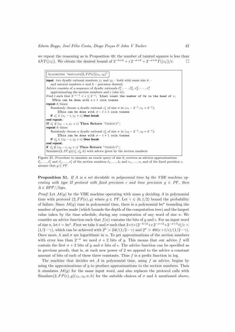
Edwin Beggs, Jose Felix Costa, Diogo Pocas & John V Tucker 42
we repeat the reasoning as in Proposition 48; the number of tainted squares is less than
4NT (|z1|). We obtain the desired bound of 2−h+2 + ε 2−σ+3 + 2−σ+3 T (|z1|)/ε.
Algorithm “simulate[2, FP (ε)](z1, z2)”
input two dyadic rational numbers z1 and z2 – both with same size k –and natural numbers σ and h – precision desired;
Advice consists of a sequence of dyadic rationals `′′1 , · · · , `′′T , r′′T , · · · , r
′′1
approximating the section numbers and ε (size σ);Find t such that 2−t−1 < ε ≤ 2−t; %Just count the number of 0s in the head of ε;
%This can be done with s+ 1 coin tosses
repeat h timesRandomly choose a dyadic rational z′1 of size σ in (z1 − 2−t, z1 + 2−t);
%This can be done with σ − t+ 1 coin tosses
if z′1 ∈ (z1 − ε, z1 + ε) then breakend repeat;If z′1 6∈ (z1 − ε, z1 + ε) Then Return “timeout”;repeat h times
Randomly choose a dyadic rational z′2 of size σ in (z2 − 2−t, z2 + 2−t);
%This can be done with σ − t+ 1 coin tosses
if z′2 ∈ (z2 − ε, z2 + ε) then breakend repeat;if z′2 6∈ (z2 − ε, z2 + ε) Then Return “timeout”;Simulate(2, IP, g)(z′1, z
′2, h) with advice given by the section numbers
Figure 21. Procedure to simulate an oracle query of size k; receives as advices approximations
`′1, . . . , `′t and r′1, . . . , r
′t of the section numbers `1, . . . , `t and r1, . . . , rt and of the fixed precision ε;
assume that g ∈ PF .
Proposition 51. If A is a set decidable in polynomial time by the VBE machine op-
erating with type II protocol with fixed precision ε and time precision g ∈ PF , then
A ∈ BPP//log?.
Proof: Let M(y) be the VBE machine operating with mass y deciding A in polynomial
time with protocol (2, FP (ε), g) where g ∈ PF . Let γ ∈ (0, 1/2) bound the probability
of failure. Since M(y) runs in polynomial time, there is a polynomial bna bounding the
number of queries made (which bounds the depth of the computation tree) and the largest
value taken by the time schedule, during any computation of any word of size n. We
consider an advice function such that f(n) contains the bits of y and ε. For an input word
of size n, let t = bna. First we take h and σ such that 3×t×(2−h+2+ε 2−σ+3+2−σ+3 t)/ε <
(1/2−γ), which can be achieved with 2h > 24t/(1/2−γ) and 2σ > 48t(ε+t/ε)/(1/2−γ).
Once more, h and σ are logarithmic in n. To get approximations of the section numbers
with error less than 2−σ we need σ + 2 bits of y. This means that our advice f will
contain the first σ + 2 bits of y and σ bits of ε. The advice function can be specified as
in previous proofs, that is, at each new power of 2 we append to the advice a constant
amount of bits of each of these three constants. Thus f is a prefix function in log.
The machine that decides set A in polynomial time, using f as advice, begins by
using the approximations of y to produce approximations to the section numbers. Then
it simulates M(y) for the same input word, and also replaces the protocol calls with
Simulate(2, FP (ε), g)(z1, z2, σ, h) for the suitable choices of σ and h mentioned above,
Computations with oracles that measure vanishing quantities 43
using as advice the approximations of the section numbers and of ε. The difference in
probabilities, by Proposition 48, is less than 2−h+2 + ε 2−σ+3 + 2−σ+3 t/ε. Then, by
Proposition 35, the difference in the probabilities of acceptance is bounded by a constant
less than 1/2−γ and so the probability that this machine gives a wrong answer is bounded
by a constant less than 1/2. Since each simulation can be done in polynomial time, this
machine also runs in polynomial time. It follows that A ∈ BPP//log?.
12. Concluding remarks
12.1. Computational theory of measurement
Measurement theory is about operations on the real world that define real numbers: see
(Hempel 1952), (Carnap 1966), and the three-volume (Krantz, Suppes, Luce & Tversky
1990). In our computational approach we have considered an idealised experimenter as a
Turing machine, and an idealised experiment to measure a physical quantity as an oracle
to the Turing machine.
Typically, to measure the value of a physical quantity as a real number we use approxi-
mations. In principle, whenever possible, the algorithm conducting the experiment should
approximate the unknown quantity by a series of experimental values that converges. The
time needed to consult the oracle is not any more a single step of computation but a num-
ber of time steps that will depend on the precision. Two-sided measurements have been
considered in (Beggs, Costa, Loff & Tucker 2008; Beggs, Costa & Tucker 2010b; Beggs,
Costa & Tucker 2010c; Beggs, Costa & Tucker 2012a; Beggs, Costa & Tucker 2012b) and
threshold experiments in (Beggs, Costa, Pocas & Tucker 2013a; Beggs, Costa, Pocas &
Tucker 2013b). The main complexity classes of Turing machines coupled with these mea-
surements have been studied here for the case of vanishing quantities. We have seen two
vanishing experiments, there are more: the Brewster angle experiment is an example of a
common physical measurement that falls into this class, while the VBE is constructed to
be simple to describe and use in theory development. What is the scope of these results?
To answer this we need to
(i) axiomatise a specification of the interface to a physical oracle, and
(ii) provide certification lemmas to check whether a given experiment actually satisfies
the oracle interface.
This is an open problem. A first attempt is (Beggs, Costa & Tucker 2014), which gave
a lower bound.
12.2. Comparing the power of oracles
The original and primary purpose of an oracle is to boost algorithms. Let us compare
the characteristics of the vanishing experiments described here with the other types of
experiments described previously – see (Beggs, Costa, Loff & Tucker 2008; Beggs, Costa &
Tucker 2010b; Beggs, Costa & Tucker 2010c; Beggs, Costa & Tucker 2012a; Beggs, Costa
& Tucker 2012b; Beggs, Costa, Pocas & Tucker 2013b). The three types of experiments
have the following common characteristics:
Edwin Beggs, Jose Felix Costa, Diogo Pocas & John V Tucker 44
— A real value is being measured.
— (characteristic 1). A query corresponds to a classical query to the oracle in the
following sense: the answer is “yes”, or “no”, or “timeout” (meaning no answer in
the given time).
— Queries express dyadic rational putative values of the concept being measured.
— The cost of the oracle to the Turing machine expresses the time required by the
experiment.‡‡
Note that characteristic 1 clarifies that the answer should be a qualitative aspect of
the experimental apparatus, e.g., a detection, and not dependent on prior measurements.
The threshold oracles introduced in (Beggs, Costa, Pocas & Tucker 2013a; Beggs, Costa,
Pocas & Tucker 2013b) have a different characteristic 1, namely:
— characteristic 2. A query corresponds to a classical query to the oracle in the
following sense: the answer is “yes”, or “timeout”.
The vanishing oracles studied in this paper differ also from characteristic 1, 2,
namely:
— characteristic 3. A query does not correspond to a classical query to the oracle in
the following sense: two queries are made at the same machine (experimenter) time;
if the oracle answers first to query number one, then it is interpreted as a “yes”, else
if the oracle answers first to query number two, then is interpreted as a “no”, and
otherwise a “timeout” or an “indistinguishable” is returned.
Figure 22 reports on lower and upper bounds of VBE machines together with the
results of our previous research on the two-sided and threshold oracles.
‡‡ Remember that the classical connection between the Turing machine and the oracle is a one step
computation.
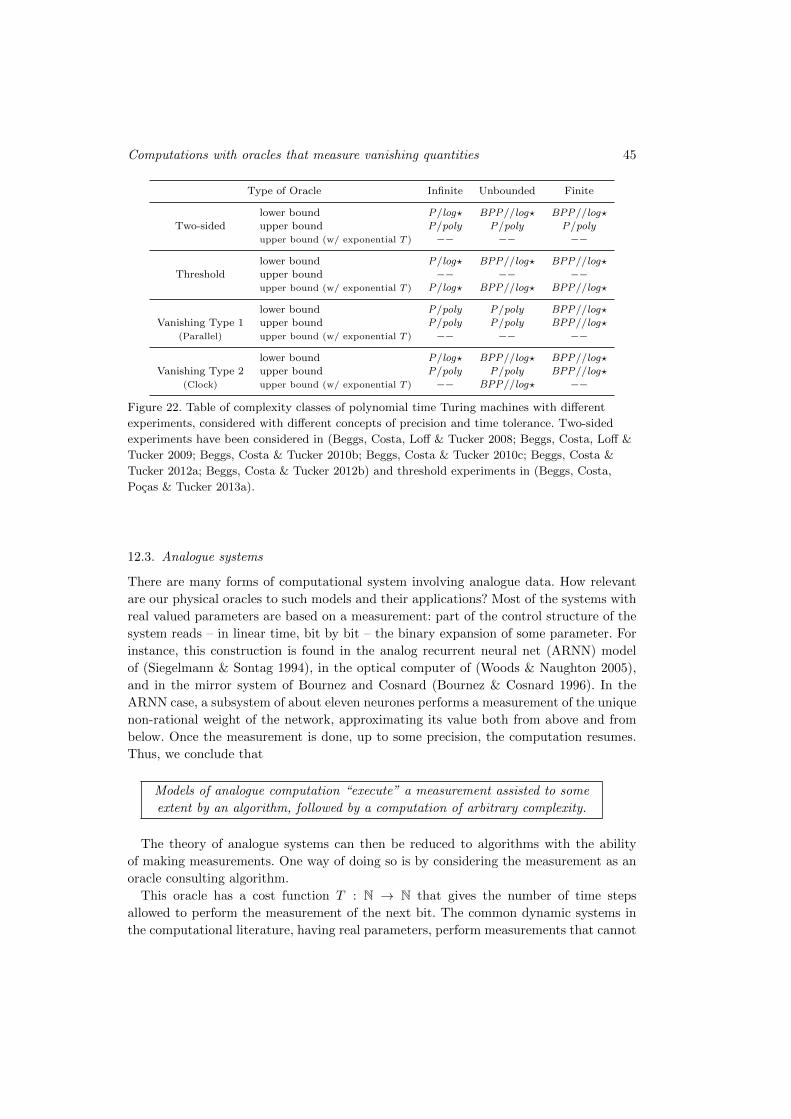
Computations with oracles that measure vanishing quantities 45
Type of Oracle Infinite Unbounded Finite
lower bound P/log? BPP//log? BPP//log?
Two-sided upper bound P/poly P/poly P/poly
upper bound (w/ exponential T ) −− −− −−
lower bound P/log? BPP//log? BPP//log?
Threshold upper bound −− −− −−upper bound (w/ exponential T ) P/log? BPP//log? BPP//log?
lower bound P/poly P/poly BPP//log?Vanishing Type 1 upper bound P/poly P/poly BPP//log?
(Parallel) upper bound (w/ exponential T ) −− −− −−
lower bound P/log? BPP//log? BPP//log?
Vanishing Type 2 upper bound P/poly P/poly BPP//log?
(Clock) upper bound (w/ exponential T ) −− BPP//log? −−
Figure 22. Table of complexity classes of polynomial time Turing machines with different
experiments, considered with different concepts of precision and time tolerance. Two-sided
experiments have been considered in (Beggs, Costa, Loff & Tucker 2008; Beggs, Costa, Loff &
Tucker 2009; Beggs, Costa & Tucker 2010b; Beggs, Costa & Tucker 2010c; Beggs, Costa &
Tucker 2012a; Beggs, Costa & Tucker 2012b) and threshold experiments in (Beggs, Costa,
Pocas & Tucker 2013a).
12.3. Analogue systems
There are many forms of computational system involving analogue data. How relevant
are our physical oracles to such models and their applications? Most of the systems with
real valued parameters are based on a measurement: part of the control structure of the
system reads – in linear time, bit by bit – the binary expansion of some parameter. For
instance, this construction is found in the analog recurrent neural net (ARNN) model
of (Siegelmann & Sontag 1994), in the optical computer of (Woods & Naughton 2005),
and in the mirror system of Bournez and Cosnard (Bournez & Cosnard 1996). In the
ARNN case, a subsystem of about eleven neurones performs a measurement of the unique
non-rational weight of the network, approximating its value both from above and from
below. Once the measurement is done, up to some precision, the computation resumes.
Thus, we conclude that
Models of analogue computation “execute” a measurement assisted to some
extent by an algorithm, followed by a computation of arbitrary complexity.
The theory of analogue systems can then be reduced to algorithms with the ability
of making measurements. One way of doing so is by considering the measurement as an
oracle consulting algorithm.
This oracle has a cost function T : N → N that gives the number of time steps
allowed to perform the measurement of the next bit. The common dynamic systems in
the computational literature, having real parameters, perform measurements that cannot
Edwin Beggs, Jose Felix Costa, Diogo Pocas & John V Tucker 46
be done in linear time. In a balance, the pans move with acceleration that depends on
the difference of masses placed in them, in a way such that the time needed to detect a
mass difference increases exponentially with the precision of the measurement, no matter
how small (yet fixed) that difference can be made. This measurement has an exponential
cost that should be considered in the complexity of the decision problem.§§
12.4. Physical systems and real number computation
The computability of physical systems has been studied from time to time over a long
period. Kreisel drew attention to the problem in (Kreisel 1974) and stimulated a wave of
interest, represented by the work of Marion Pour El and Ian Richards, e.g., the papers
(Pour-El 1974; Pour-El & Richards 1979; Pour-El & Richards 1981) and the monograph
(Pour-El & Richards 1989). The equations of physics constitute a vast subject domi-
nating Mathematical Analysis. The computable analysis of the equations of physics is
an essential activity, one that goes hand-in-hand with modelling systems under various
assumptions. Modelling requires persistence – Pour El and Richard’s striking and influen-
tial non-computability results are complemented by computability results in (Weihrauch
and Zhong 2002). Today’s literature on the computability of mathematical models of
physical systems is substantial, and the literature on computable analysis, where the
tools for this programme are to be found, is very considerable.
However, the approach here is not to start with established equations but with thinking
about physical systems. Questions arise from exploring physical situations: how does data
picture them, and how are operational aspects of physical systems to be theorised and
modelled mathematically? Our interest began with an extreme approach in which we
sought to exclude computability theory, attempting to develop algorithmic notions – data
and operations – from physical processes. This required a methodology and an interest
in physical models, e.g., in (Beggs and Tucker 2006; Beggs and Tucker 2007a; Beggs
and Tucker 2007b). The combination of computability theory and physical models for
physical oracles has enabled us to create a second, new approach to the computability of
physical systems that introduces new and influential notions and questions. For example,
the simple question, what effect does the act of measurement have on a real number
computation? Any physical experiment reveals that the using the real number involves:
(i) subtle issues of precision;
(ii) cost of consultation – e.g., the fact that exponential time on the size of the query
is common in Physics;
(iii) stochastic behaviour.
The physical oracle answers queries in a time T : N → N, dependent upon the size
of the query, modelling the fact that successive approximations have a cost that is not
necessarily linear in the number of bits of precision obtained.
§§ In the non-analytic piecewise linear neural net case, the cost function is like the common oracle Turingmachine: one step consultation device, since any further bit has the constant cost of k transitions, for
some constant k ∈ N – see (Siegelmann & Sontag 1994). This is due to the fact that the activation
function is piecewise linear instead of the common analytic sigmoid.
Computations with oracles that measure vanishing quantities 47
For those seeking the clarity and stability of a pure mathematical understanding of
what are mathematical theorems, the combination – or intrusion – of physical models
gets in the way of a pure theory of real number oracles that should abstract from and
be applicable to physical measurements. However, the use of physical oracles should
be considered a strength of our approach, and necessary at least at this stage of our
understanding.
In the case of two-sided experiments, of which we have accumulated many physical
examples, our theories changed and grew quite surprisingly. For example, one can contrast
the early analysis of the wedge in (Beggs and Tucker 2007b; Beggs, Costa, Loff & Tucker
2008) with its subsequent treatment in (Beggs, Costa & Tucker 2012b): this was made
possible by our experience working on with the collider experiment in (Beggs, Costa &
Tucker 2010b). Collecting different physical oracles has been hugely productive, and the
new classification of experiments in (Beggs, Costa & Tucker 2014) comes directly from
thinking about and analysing physical experiments.
For the pure mathematician, these experiments may seem to be baggage: easy experi-
ments seem unnecessary and complicated experiments vexing. But for our scientific work
they were, and continue to be, essential. Certainly, after collecting many two-sided ex-
periments we provided a more general axiomatic approach to the computational power
theorems (Beggs, Costa & Tucker 2012a). However, that analysis required subtle cer-
tification lemmas about physical models to enable the general theorems to be applied.
In due course we have no doubt that interesting pure mathematics will emerge, but the
time is not right. Indeed, as we have looked at more complicated physical processes, we
have found new technical notions and tricks (timing and boundary numbers in this paper
being an example). Thus, our program is a work in progress, and, so far, it is true to say
that progress can be attributed to engagement with physical examples.
Acknowledgements. The research of Jose Felix Costa is supported by Fundacao para
a Ciencia e Tecnologia, PEst – OE/MAT/UI0209/2011.
References
Jose Luis Balcazar, Josep Dıas & Joaquim Gabarro (1990). Structural Complexity I, second
edition, Springer-Verlag.
Edwin Beggs, Jose Felix Costa, Bruno Loff, and John V. Tucker (2008). Computational com-
plexity with experiments as oracles, Proceedings of the Royal Society, Series A (Mathematical,
Physical and Engineering Sciences), 464 (2098):2777-2801.
Edwin Beggs, Jose Felix Costa, Bruno Loff, and John V. Tucker (2009). Computational com-
plexity with experiments as oracles II. Upper bounds, Proceedings of the Royal Society, Series
A (Mathematical, Physical and Engineering Sciences), 465 (2105):1453–1465.
Edwin Beggs, Jose Felix Costa, Diogo Pocas, and John V. Tucker (2013a). On the power
of threshold measurements as oracles, In Giancarlo Mauri, Alberto Dennunzio, Luca Man-
zoni, and Antonio E. Porreca, editors, Unconventional Computation and Natural Computation
(UCNC 2013), vol. 7956 of Lecture Notes in Computer Science, pages 6–18. Springer-Verlag.
Edwin Beggs, Jose Felix Costa, Diogo Pocas, and John V. Tucker (2013b). Oracles that measure
thresholds: the Turing machine and the broken balance, Journal of Logic and Computation,
23 (6):1155-1181.

Edwin Beggs, Jose Felix Costa, Diogo Pocas & John V Tucker 48
Edwin Beggs, Jose Felix Costa, and John V. Tucker (2010a). Computational Models of Mea-
surement and Hempel’s Axiomatization, In Arturo Carsetti, editor, Causality, Meaningful
Complexity and Knowledge Construction, vol. 46 of Theory and Decision Library A, pages
155–184, Springer-Verlag.
Edwin Beggs, Jose Felix Costa, and John V. Tucker (2010b). Limits to measurement in experi-
ments governed by algorithms. Mathematical Structures in Computer Science, 20 (06):1019–
1050. Special issue on Quantum Algorithms, editor Salvador Elıas Venegas-Andraca.
Edwin Beggs, Jose Felix Costa, and John V. Tucker (2010c). Physical oracles: The Turing
machine and the Wheatstone bridge, Studia Logica, 95 (1–2):279–300. Special issue on
Contributions of Logic to the Foundations of Physics, editors D. Aerts, S. Smets & J. P. Van
Bendegem.
Edwin Beggs, Jose Felix Costa, and John V. Tucker (2012a). Axiomatising physical experi-
ments as oracles to algorithms, Philosophical Transactions of the Royal Society, Series A
(Mathematical, Physical and Engineering Sciences), 370 (12):3359–3384.
Edwin Beggs, Jose Felix Costa, and John V. Tucker (2012b). The impact of models of a physical
oracle on computational power, Mathematical Structures in Computer Science, 22 (5):853–
879. Special issue on Computability of the Physical, editors Cristian S. Calude and S. Barry
Cooper.
Edwin Beggs, Jose Felix Costa, and John V. Tucker (2014). Three forms of physical measurement
and their computability, Reviews of Symbolic Logic, 7 (4):618-646.
Edwin Beggs and John V. Tucker (2006). Embedding infinitely parallel computation in Newto-
nian kinematics, Applied Mathematics and Computation, 178 (1):25–43.
Edwin Beggs and John V. Tucker (2007a). Can Newtonian systems, bounded in space, time,
mass and energy compute all functions? Theoretical Computer Science, 371 (1):4–19
Edwin Beggs and John V. Tucker (2007b). Experimental computation of real numbers by
Newtonian machines, Proceedings of the Royal Society, Series A (Mathematical, Physical and
Engineering Sciences), 463 (2082):1541–1561.
George A. Bekey and Walter J. Karplus (1968). Hybrid Computation, John Wiley & Sons.
Max Born and Emil Wolf (1964). Principles of Optics. Electromagnetic Theory of Propagation,
Interference and Diffraction of Light, Pergamon Press, second (revised) edition.
Olivier Bournez and Michel Cosnard (1996). On the computational power of dynamical systems
and hybrid systems, Theoretical Computer Science, 168 (2):417–459.
Rudolf Carnap (1966). Philosophical Foundations of Physics, Basic Books.
Robert Geroch and James B Hartle (1986). Computability and physical theories, Foundations
of Physics, 16 (6):533–550.
Carl G. Hempel (1952). Fundamentals of concept formation in empirical science, International
Encyclopedia of Unified Science, vol. 2 no. 7, Chicago UP.
David H. Krantz, Patrick Suppes, R. Duncan Luce, and Amos Tversky (1990). Foundations of
Measurement, Academic Press, vol. 1 (1971), vol. 2 (1989) and vol. 3 (1990).
Georg Kreisel (1974). A notion of mechanistic theory, Synthese, 47:9–24.
Arno Pauly (2009). Representing measurement results, Journal of Universal Computer Science,
15 (6):1280–1300.
Arno Pauly and Martin Zeigler (2013). Relative computability and uniform continuity of rela-
tions, Journal of Logic and Analysis 5 (7):139.
Marion Pour-El (1974). Abstract computability and its relations to the general purpose analog
computer, Transactions of the American Mathematical Society, 199:1–28.
Marion Pour-El and Ian Richards (1979). A computable ordinary differential equation which
possesses no computable solution, Annals of Mathematical Logic, 17 :61 – 90.
Computations with oracles that measure vanishing quantities 49
Marion Pour-El and Ian Richards (1981). The wave equation with computable initial data such
that its unique solution is not computable, Advances in Mathematics, 39(4):215–239.
Marion Pour-El and Ian Richards (1989). Computability in Analysis and Physics, Perspectives
in Mathematical Logic, Springer-Verlag, 1989.
Hava T. Siegelmann and Eduardo D. Sontag (1994). Analog computation via neural networks,
Theoretical Computer Science, 131(2):331–360.
Klaus Weihrauch (2000). Computable Analysis, Springer-Verlag.
Klaus Weihrauch and Ning Zhong (2002). Is wave propagation computable or can wave comput-
ers beat the Turing machine?, Proceedings of the London Mathematical Society, 85 (2):312–
332.
Damien Woods and Thomas J. Naughton (2005). An optical model of computation, Theoretical
Computer Science, 334 (1-3):227–258.
Martin Ziegler (2009). Physically-relativized Church-Turing hypotheses: Physical foundations
of computing and complexity theory of computational physics, Applied Mathematics and
Computation, 215 (4):1431–1447.