computational tools for probing interactions in...
TRANSCRIPT

Journal of Educational and Behavioral StatisticsWinter 2006, Vol. 31, No. 4. pp. 437-448
Computational Tools for Probing Interactionsin Multiple Linear Regression, Multilevel Modeling,
and Latent Curve Analysis
Kristopher J. PreacherPatrick J. CurranDaniel J. Bauer
University of North Carolina at Chapel Hill
Simple slopes, regions of significance, and confidence bands are commonly usedto evaluate interactions in multiple linear regression (MLR) models, and the use ofthese techniques has recently been extended to multilevel or hierarchical linear
modeling (HLM) and latent curve analysis (LCA). However, conducting thesetests andplotting the conditional relations is often a tedious and error-prone task.This article provides an overview of methods used to probe interaction effects anddescribes a unified collection offreely available online resources that researchers
can use to obtain significance testsforsimple slopes, compute regions of significance,and obtain confidence bands for simple slopes across the range of the moderatorin the MLR, HLM, and LCA contexts. Plotting capabilities are also provided.
Keywords: interaction, Johnson-Neyman technique, latent curve analysis, multilevel mod-eling, multiple regression
Hypotheses involving multiplicative interaction or moderation effects are com-mon in the social sciences. Interaction effects are typically evaluated by testing the
significance of a multiplicative term consisting of the product between two or morepredictor variables controlling for associated lower order main effects (e.g., Cohen,
1978). When a significant interaction is found, it is common to further decompose
or "probe" this conditional effect to better understand the structure of the relation
(e.g., Aiken & West, 1991).
Although interactions arise in many seemingly disparate analytic frameworks,
interactions within these frameworks share a common computational form. Ina series of articles, we have explored these computational linkages within three
major analytic frameworks: the multiple linear regression (MLR) model (Bauer &
This work was funded in part by National Institute on Drug Abuse Grant DA16883 awarded toKristopher J. Preacher and Grant DA13148 awarded to Patrick J. Curran. The authors thank membersof the Carolina Structural Equation Modeling Group for their valuable input. The online resourcesdescribed in this article for computing simple slopes and regions of significance are available online at:http://www.quantpsy.org/.
437
Preacher, Curran, and Bauer
Curran, 2005), the random effects multilevel/hierarchical linear model (HLM)
(Bauer & Curran, 2005; Curran, Bauer, & Willoughby, 2006), and the structural
equation-based latent curve analysis (LCA) model (Curran, Bauer, & Willoughby,
2004). In these articles we also describe a variety of specific tests that we believe are
helpful in the probing of complex interaction terms in MLR, HLM, and LCA.
Although we view these tests as potentially powerful and widely applicable, many
of the required values are computed by hand and these calculations can be quite cum-
bersome and consequently error-prone. The complexity of many of these tests also
may substantially reduce the likelihood that these methods will be used in practice.
Our goal here is to integrate across our three prior articles and capitalize on the
shared computational linkages in testing interactions in order to develop a set of freely
available online tools that automate the testing and plotting of these complex effects.
We begin by presenting a single shared notational system to define the general
estimation of two-way interactions. This general expression can equivalently define
higher order interactions stemming from MLR, HLM, and LCA. We briefly review
some methods available for the further probing and plotting of these effects. We
present online calculators designed to be easily accessible and to automate the
calculation of a variety of tests for probing interactions described in Bauer and Curran
(in press) and Curran et al. (2004, in press). Finally, we demonstrate our calculators
by probing an interaction in MLR.
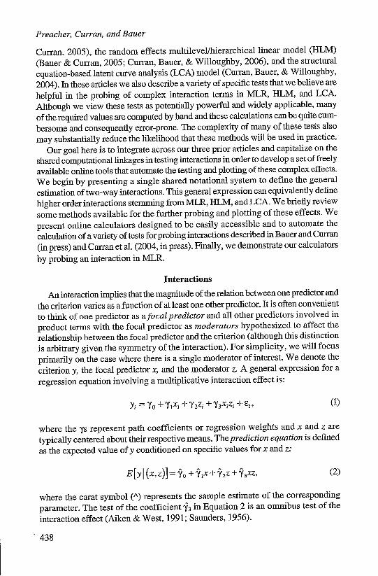
Interactions
An interaction implies that the magnitude of the relation between one predictor and
the criterion varies as a function of at least one other predictor. It is often convenient
to think of one predictor as afocal predictor and all other predictors involved in
product terms with the focal predictor as moderators hypothesized to affect the
relationship between the focal predictor and the criterion (although this distinction
is arbitrary given the symmetry of the interaction). For simplicity, we will focus
primarily on the case where there is a single moderator of interest. We denote the
criterion y, the focal predictor x, and the moderator z. A general expression for a
regression equation involving a multiplicative interaction effect is:
Yi = YO + YlXi + 72 Z i + y 3xizi + 6"i (1)
where the ys represent path coefficients or regression weights and x and z are
typically centered about their respective means. The prediction equation is defined
as the expected value of y conditioned on specific values for x and z:
E [yI (x, z)] = ý + j'x + 2z + Q3 xz, (2)
where the carat symbol (A) represents the sample estimate of the corresponding
parameter. The test of the coefficient y3 in Equation 2 is an omnibus test of the
interaction effect (Aiken & West, 1991; Saunders, 1956).
438
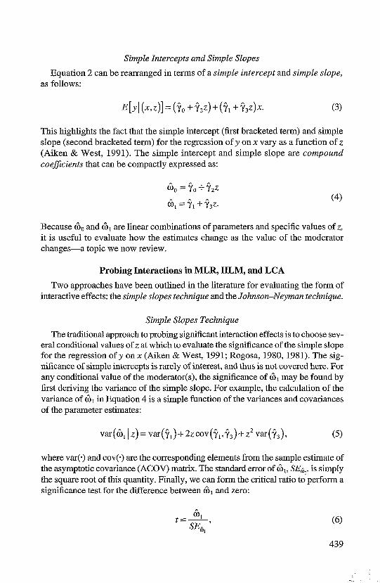
Simple Intercepts and Simple Slopes
Equation 2 can be rearranged in terms of a simple intercept and simple slope,as follows:
E[yI (XIZ)] = (j' + 2Z)+(il + j 3z)x. (3)
This highlights the fact that the simple intercept (first bracketed term) and simpleslope (second bracketed term) for the regression of y on x vary as a function of z(Aiken & West, 1991). The simple intercept and simple slope are compoundcoefficients that can be compactly expressed as:
COO = 'o + y2z
,1 Y 1 + 73 Z. (4)
Because 60 and 61 are linear combinations of parameters and specific values of z,it is useful to evaluate how the estimates change as the value of the moderatorchanges-a topic we now review.
Probing Interactions in MLR, HLM, and LCA
Two approaches have been outlined in the literature for evaluating the form ofinteractive effects: the simple slopes technique and the Johnson-Neyman technique.
Simple Slopes Technique
The traditional approach to probing significant interaction effects is to choose sev-eral conditional values of z at which to evaluate the significance of the simple slopefor the regression of y on x (Aiken & West, 1991; Rogosa, 1980, 1981). The sig-nificance of simple intercepts is rarely of interest, and thus is not covered here. Forany conditional value of the moderator(s), the significance of 6) may be found byfirst deriving the variance of the simple slope. For example, the calculation of thevariance of 61 in Equation 4 is a simple function of the variances and covariancesof the parameter estimates:
var (Co, I z) = var ( #,) + 2z cov('l,• + z' var(' ) (5)
where var(.) and cov(-) are the corresponding elements from the sample estimate ofthe asymptotic covariance (ACOV) matrix. The standard error of 6), SE6,, is simplythe square root of this quantity. Finally, we can form the critical ratio to perform asignificance test for the difference between Co1 and zero:
t = -n (6)SE614
439

Preacher, Curran, and Bauer
the significance of which is determined by comparing the obtained t to a t distri-bution at the desired cx level and degrees of freedom (df) = N - p - 1, where N isthe sample size and p is the number of predictors.
In order to employ the simple slopes method described above, conditional valuesof the moderator, denoted cv2, must be chosen (what Rogosa, 1980, refers to as the"pick-a-point" approach). For dichotomous moderators, cv, assumes values of thedichotomy (usually 0 and 1). For continuous moderators, the specific choices forcv, are less obvious and may be any value of scientific interest. In the absence oftheoretically meaningful values. Cohen and Cohen (1983) recommend choosingvalues at the mean of z and at 1 SD above and below the mean of z.
The Johnson-Neyman Technique
Despite its broad usefulness, the simple slopes method has an important limitation:the choices of cvz are ultimately arbitrary. An alternative is the Johnson-Neyman(J-N) technique (Johnson & Neyman, 1936). The J-N technique essentially worksbackwards from the critical ratio defined in Equation 6. Instead of calculating tas a function of CoI and SE6, and a chosen value cv,, the J-N technique calcu-lates the cv, that yields a specific t (usually the critical t value to obtain ap valueof .05 at a given df). The conditional values that are returned by the J-N techniquedefine the regions of significance on z, and represent the range of z within whichthe simple slope of y on x is significantly different from zero at the chosen (X.Assuming solutions exist, the result will be two values: upper and lower bound-aries of the region of significance. In many cases, the regression of y on the focalpredictor is significant at values of the moderator that are less than the lowerbound and greater than the upper bound, while the regression is nonsignificantat values of the moderator falling within the region. However, there are somecases in which the opposite holds (i.e., the significant slopes fall within the regionboundaries).
Confidence Bands
Both the simple slopes and J-N techniques rely on traditional null hypothesistesting logic. It is well known that confidence intervals (CIs) provide more infor-mation than hypothesis tests, and methodologists increasingly recommend the useof CIs in addition to, or in place of, hypothesis tests whenever possible (Wilkinson& APA TaskForce, 1999). The general formula for a 100 x (1 - ox)% CI for a simpleslope (Cohen, Cohen, West, & Aiken, 2003) is:
CI(., = O1 ± tc,SE6,. (7)
Because the formula for SE6, relies on particular choices for z, CI6, varies as afunction of the moderator. When CIB, is plotted across all relevant values of z, theresult is a pair of confidence bands (Bauer & Curran, in press; Rogosa, 1980, 1981;Tate, 2004).
440

Interactions in HLM
The same methods used to represent interactions in MLR in terms of simpleintercepts and simple slopes (i.e., Equation 4) can also be used to represent inter-actions in HLM and LCA. In each modeling context, the dependency of the crite-rion on the focal predictor can be represented as a function of the moderator(s) bydefining two compound coefficients, 60 and Co.
In HLM with two predictors, interactions may occur between two Level 1predictors (Case 1), between two Level 2 predictors (Case 2), or between Level 1and Level 2 predictors (Case 3, or cross-level interaction). A cross-level (Case 3)interaction occurs when the random slope of a Level 1 predictor is predicted bya Level 2 predictor. This last type of interaction is probably most commonlyencountered in HLM, so we will focus on it here. In cross-level interactions, eitherthe Level I or Level 2 predictor may be chosen as the focal predictor. Typically,however, it is the Level 1 predictor that is chosen to be the focal predictor. TheLevel 1 equation is:
YYu = P0j + PjxY ,+ r,, (8)
where xy represents the Level 1 predictor for the ith individual nested within thejth group. Because the intercept and slope in HLM are viewed as random variables,they can be expressed in the Level 2 equations:
3Oj Y700 + Y01wj + 10j
Ou = Y10 + nwj + u(,
where wj represents the Level 2 predictor for thejth group. Substituting the Level 2equations into Equation 8 results in the reduced form expression:
i=(YOO + OXU + + Y) + (Uoj + UijXY + 0) (10)
The prediction equation derived from Equation 10 is:
In Equation 11, the test of the coefficient 'x Iis an omnnibus test of the interaction effect.Defining x as the focal predictor and w as the moderator results in the predictionequation:
E[yI (x,w)] + (r I w)+ ( j +
441

Preacher, Curran, and Bauer
This rearrangement again highlights the simple intercept and slope of the regres-
sion of y on x at specific values of w. Using the same notation as before, these are
defined as
6= '00 + '01w(12)
The simple slope, 6 , may be interpreted and evaluated using the simple slopes,
regions of significance, and confidence band strategies described earlier.
Interactions in LCA
The same methods used to represent interaction effects in MLR and BILM can
also be used to represent interactions in LCA, an application of structural equation
modeling (SEM). LCA represents the repeated measures of a dependent variable y
as a function of latent factors that capture different aspects of change, typically an
intercept factor (ih) and one or more slope factors (1p). The equation for the
repeated measures of y for individual i at time t is:
Yit = T1ai + 2'r-fip + it,, (13)
where ?. represents a fixed factor loading on the slope factor corresponding to a
value of the time metric (see Curran et al., 2004, for details).
The factors representing the intercept and slope then often serve as endogenous
(dependent) variables in other model equations. For instance, the latent curve
factors could be regressed on the exogenous predictor x:
Ta R.+ YAX + ýCai11PI = ttP + 72X! + ýPi- + ~(14)
The reduced form equation is then:
Yit = (ý. + + 7Xy1x + 72X1x') + (ýai + ý1ik' + it). (15)
The fixed component (first part) of Equation 15 contains an intercept term (i.e., ,
conditional main effects for time (i.e., pp) and the exogenous predictor x (i.e., yi),
and the interaction of time andx (i.e., y2). Thus, the regression of y on time depends
in part on the level of x, so x can be considered the moderator and time the focal
predictor. Taking the expectation of Equation 15 and rearranging yields a prediction
equation that highlights the role of x as a moderator of the time effect (the slope of
the individual trajectories):
E[yf+ (+,x)] ( (j' + 1- 12X)X,. (16)
442
Tools for Probing Interaction Effects
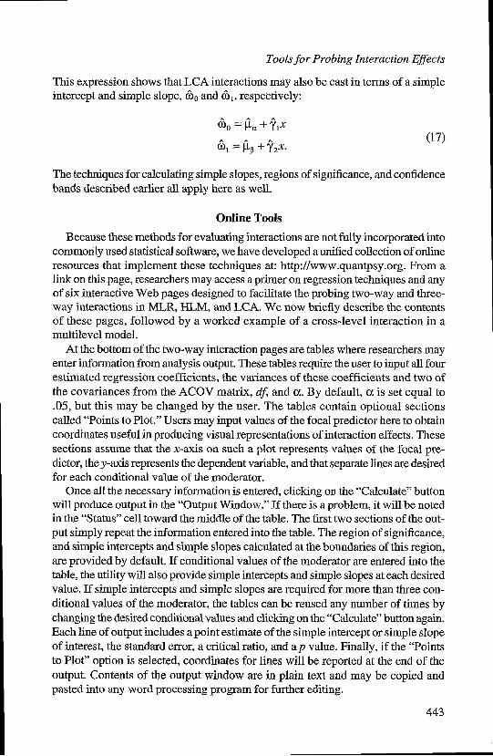
This expression shows that LCA interactions may also be cast in terms of a simpleintercept and simple slope, &0 and 61, respectively:
0 + YXC0 = +'y 2x. (17)
The techniques for calculating simple slopes, regions of significance, and confidencebands described earlier all apply here as well.
Online Tools
Because these methods for evaluating interactions are not fully incorporated intocommonly used statistical software, we have developed a unified collection of onlineresources that implement these techniques at: http://www.quantpsy.org. From alink on this page, researchers may access a primer on regression techniques and anyof six interactive Web pages designed to facilitate the probing two-way and three-way interactions in MLR, HLM, and LCA. We now briefly describe the contentsof these pages, followed by a worked example of a cross-level interaction in amultilevel model.
At the bottom of the two-way interaction pages are tables where researchers mayenter information from analysis output. These tables require the user to input all fourestimated regression coefficients, the variances of these coefficients and two ofthe covariances from the ACOV matrix, df, and c. By default, a is set equal to.05, but this may be changed by the user. The tables contain optional sectionscalled "Points to Plot." Users may input values of the focal predictor here to obtaincoordinates useful in producing visual representations of interaction effects. Thesesections assume that the x-axis on such a plot represents values of the focal pre-dictor, the y-axis represents the dependent variable, and that separate lines are desiredfor each conditional value of the moderator.
Once all the necessary information is entered, clicking on the "Calculate" buttonwill produce output in the "Output Window." If there is a problem, it will be notedin the "Status" cell toward the middle of the table. The first two sections of the out-put simply repeat the information entered into the table. The region of significance,and simple intercepts and simple slopes calculated at the boundaries of this region,are provided by default. If conditional values of the moderator are entered into thetable, the utility will also provide simple intercepts and simple slopes at each desiredvalue. If simple intercepts and simple slopes are required for more than three con-ditional values of the moderator, the tables can be reused any number of times bychanging the desired conditional values and clicking on the "Calculate" button again.Each line of output includes a point estimate of the simple intercept or simple slopeof interest, the standard error, a critical ratio, and a p value. Finally, if the "Pointsto Plot" option is selected, coordinates for lines will be reported at the end of theoutput. Contents of the output window are in plain text and may be copied andpasted into any word processing program for further editing.
443

Preacher, Curran, and Bauer
The tables for three-way interactions are considerably larger than the two-way
interaction tables, primarily because many more elements of the ACOV matrix
must be entered, but they are entirely analogous to the two-way tables. The only
significant difference is that the three-way interaction tables enable the user to
request simple intercepts and simple slopes of y on x at conditional values of both
moderators z and w.The HLM two-way interaction tool has three separate tables for the Case 1, Case 2,
and Case 3 interactions described above. In addition, the user has the option of
entering custom dffor tests of simple intercepts, tests of simple slopes, or both simple
intercepts and simple slopes. If either of these boxes is left blank, asymptotic z tests
will be conducted instead of t tests. The HEM three-way interaction tool is analogous
to the MLR three-way interaction tool. However, it is limited to the case in which
there is a cross-level interaction between a single Level 1 (focal) predictor and two
Level 2 moderators.The LCA interaction tools are similar to the MLR and HLM tools. The LCA
two-way interaction tool contains two tables: one table is used for situations
involving time as the focal predictor and the other is used for situations involving
an exogenous predictor of slopes as the focal predictor. The LCA three-way inter-
action tool treats time as the focal predictor, and allows users to request simple
intercepts and simple slopes at conditional values of two exogenous predictors, x,
and x2."If conditional values are entered for the moderator(s), these tools also produce
graphs of the simple regression lines for the focal predictor at those values. Specif-
ically, they generate R syntax that can be submitted to an Rweb server (or to a local
"R application for better resolution) via the click of a button to generate the plot.
"R syntax is also generated for the plotting of confidence bands, which again can be
submitted to R or Rweb with the click of a button to produce the plot.
An Example
We now provide an illustration of the MLR two-way interaction tool. For this
example we rely on data from the National Longitudinal Survey of Youth (NLSY).
Data consist of scores on measures of math ability (math; the Peabody Individual
Achievement Test math subsection) and associated predictor variables from 956 stu-
dents (52% female) ranging in age from 59 to 156 months. Of interest in this analysis
was the finding of a significant interaction between the predictors antisocial behavior
(antisocial) and hyperactivity (both centered) in predicting math test scores. The
model is of the same form as Equations 1-3, where antisocial takes the place of
x and hyperactivity takes the place of z, except that age, sex, grade, and minority
status were added as covariates. The results from fitting the model are reported in
Table 1. The main effect of antisocial is positive but nonsignificant, and the main
effect of hyperactive is negative and significant. In addition, the significant nega-
tive coefficient associated with the interaction term (-0.3977) indicates that the
relationship between antisocial and math tends to be more strongly negative for
individuals with higher overall hyperactivity.
444
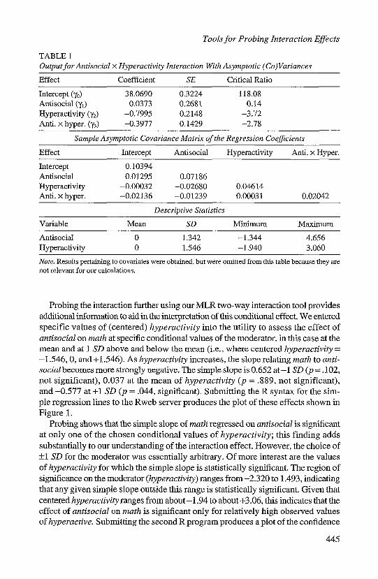
Tools for Probing Interaction Effects
TABLE 1Outputfor Antisocial x Hyperactivity Interaction With Asymptotic (Co) Variances
Effect Coefficient SE Critical Ratio
Intercept (yo) 38.0690 0.3224 118.08Antisocial (yj) 0.0373 0.2681 0.14Hyperactivity (y2) -0.7995 0.2148 -3.72Anti. x hyper. (y3) -0.3977 0.1429 -2.78
Sample Asymptotic Covariance Matrix of the Regression Coefficients
Effect Intercept Antisocial Hyperactivity Anti. x Hyper.
Intercept 0.10394Antisocial 0.01295 0.07186Hyperactivity -0.00032 -0.02680 0.04614Anti. x hyper. -0.02136 -0.01239 0.00031 0.02042
Descriptive Statistics
Variable Mean SD Minimum Maximum
Antisocial 0 1.342 -1.344 4.656Hyperactivity 0 1.546 -1.940 3.060
Note. Results pertaining to covariates were obtained, but were omitted from this table because they arenot relevant for our calculations.
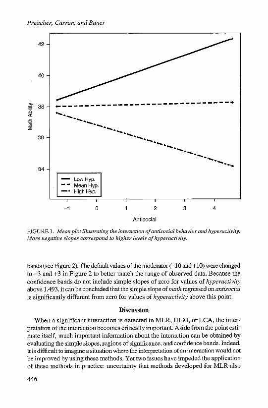
Probing the interaction further using our MLR two-way interaction tool providesadditional information to aid in the interpretation of this conditional effect. We enteredspecific values of (centered) hyperactivity into the utility to assess the effect ofantisocial on math at specific conditional values of the moderator, in this case at themean and at 1 SD above and below the mean (i.e., where centered hyperactivity =-1.546, 0, and +1.546). As hyperactivity increases, the slope relating math to anti-social becomes more strongly negative. The simple slope is 0.652 at-1 SD (p -. 102,not significant), 0.037 at the mean of hyperactivity (p = .889, not significant),and -0.577 at +1 SD (p = .044, significant). Submitting the R syntax for the sim-ple regression lines to the Rweb server produces the plot of these effects shown inFigure 1.
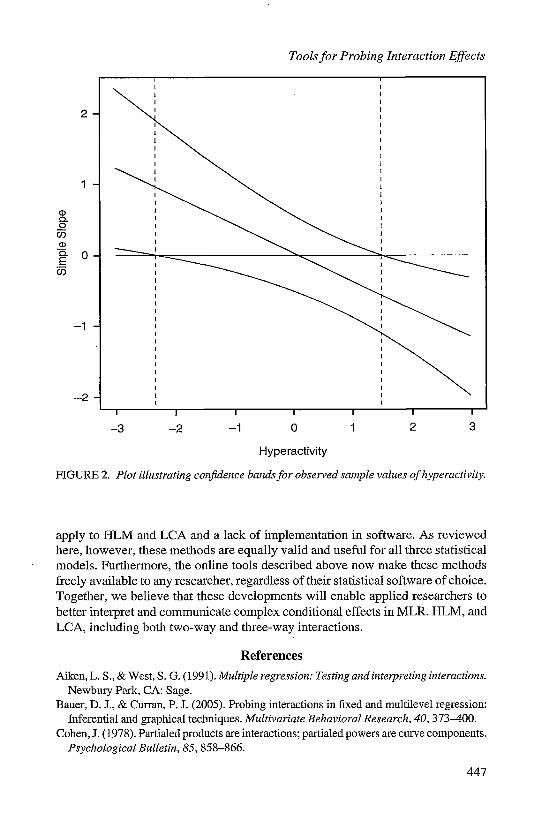
Probing shows that the simple slope of math regressed on antisocial is significantat only one of the chosen conditional values of hyperactivity; this finding addssubstantially to our understanding of the interaction effect. However, the choice of±1 SD for the moderator was essentially arbitrary. Of more interest are the valuesof hyperactivity for which the simple slope is statistically significant. The region ofsignificance on the moderator (hyperactivity) ranges from -2.320 to 1.493, indicatingthat any given simple slope outside this range is statistically significant. Given thatcentered hyperactivity ranges from about -1.94 to about +3.06, this indicates that theeffect of antisocial on math is significant only for relatively high observed valuesof hyperactive. Submitting the second R program produces a plot of the confidence
445
Preacher, Curran, and Bauer
42-
40
S38 *- -. .. -" --- --- ----2Z
36 -
34-
Low Hyp.-- Mean Hyp.
High Hyp.I I I l I I
-1 0 1 2 3 4
Antisocial
FIGURE 1. Mean plot illustrating the interaction of antisocial behavior and hyperactivity.More negative slopes correspond to higher levels of hyperactivity.
bands (see Figure 2). The default values of the moderator (-10 and +10) were changedto -3 and +3 in Figure 2 to better match the range of observed data. Because theconfidence bands do not include simple slopes of zero for values of hyperactivityabove 1.493, it can be concluded that the simple slope of math regressed on antisocial
is significantly different from zero for values of hyperactivity above this point.
Discussion
When a significant interaction is detected in MLR, HLM, or LCA, the inter-pretation of the interaction becomes critically important. Aside from the point esti-mate itself, much important information about the interaction can be obtained byevaluating the simple slopes, regions of significance, and confidence bands. Indeed,it is difficult to imagine a situation where the interpretation of an interaction would not
be improved by using these methods. Yet two issues have impeded the applicationof these methods in practice: uncertainty that methods developed for MLR also
446
Tools for Probing Interaction Effects
2-
1 -
0-
-1 -
-2 -
I I I I I I I
-3 -2 -1 0 1 2 3
Hyperactivity
FIGURE 2. Plot illustrating confidence bands for observed sample values of hyperactivity.
apply to HLM and LCA and a lack of implementation in software. As reviewedhere, however, these methods are equally valid and useful for all three statisticalmodels. Furthermore, the online tools described above now make these methodsfreely available to any researcher, regardless of their statistical software of choice.Together, we believe that these developments will enable applied researchers tobetter interpret and communicate complex conditional effects in MLR, HLM, andLCA, including both two-way and three-way interactions.
References
Aiken, L. S., & West, S. G. (199 1). Multiple regression: Testing and interpreting interactions.Newbury Park, CA: Sage.
Bauer, D. J., & Curran, P. J. (2005). Probing interactions in fixed and multilevel regression:Inferential and graphical techniques. Multivariate Behavioral Research, 40, 373-400.
Cohen, J. (1978). Partialed products are interactions; partialed powers are curve components.Psychological Bulletin, 85, 858-866.
447
(D0-0C,)0)
E
Preacher, Curran, and Bauer
Cohen, J., & Cohen, P. (1983). Applied multiple regression/correlation analyses for thebehavioral sciences (2nd ed.). Hillsdale, NJ: Erlbaunm.
Cohen, J., Cohen, P., West, S. G., & Aiken, L. S. (2003). Applied multiple regressionlcorrelation analysis for the behavioral sciences (3rd ed.). Hillsdale, NJ: Erlbaum.
Curran, P. J., Bauer, D. J., & Willoughby, M. T. (2004). Testing main effects and interactionsin latent curve analysis. Psychological Methods, 9(2), 220-237.
Curran, P. J., Bauer, D. J., & Willoughby, M. T. (2006). Testing and probing interactionsin hierarchical linear growth models. In C. S. Bergeman & S. M. Boker (Eds.), The NotreDame Series on Quantitative Methodology: Vol. 1. Methodological issues in agingresearch (pp. 99-129). Mahwah, NJ: Erlbaum.
Johnson, P. 0., & Neyman, J. (1936). Tests of certain linear hypotheses and their applicationsto some educational problems. Statistical Research Memoirs, 1, 57-93.
Rogosa, D. (1980). Comparing nonparallel regression lines. Psychological Bulletin, 88,307-321.
Rogosa, D. (1981). On the relationship between the Johnson-Neyman region of significanceand statistical tests of parallel within group regressions. Educational and PsychologicalMeasurement, 41, 73-84.
Saunders, D. R. (1956). Moderator variables in prediction. Educational and PsychologicalMeasurement, 16, 209-222.
Tate, R. (2004). Interpreting hierarchical linear and hierarchical generalized linear modelswith slopes as outcomes. The Journal of Experimental Education, 73, 71-95.
Wilkinson, L., & the APA Task Force on Statistical Inference. (1999). Statistical methods inpsychology journals: Guidelines and explanations. American Psychologist, 54(8), 594-604.
Authors
KRISTOPHER J. PREACHER is now Assistant Professor of Quantitative Psychology atthe University of Kansas, 1415 Jayhawk Blvd., Room 426, Lawrence, KS 66045-7556;[email protected]. His areas of specialization include factor analysis, structural equationmodeling, multilevel modeling, growth curve analysis, model fit, and the assessment ofmediation and moderation effects.
PATRICK J. CURRAN is a Professor in the L. L. Thurstone Psychometric Laboratory inthe Department of Psychology at the University of North Carolina at Chapel Hill,CB #3270 Davie Hall, Chapel Hill, NC 27599-3270; [email protected]. His areas of spe-cialization are structural equation modeling and multilevel modeling, particularly as appliedto longitudinal data.
DANIEL J. BAUER is Assistant Professor of Psychology, Department of Psychology,University of North Carolina at Chapel Hill, CB #3270 Davie Hall, Chapel Hill, NC27599-3270; [email protected]. His areas of specialization are mixed-effects mod-els, structural equation models, and finite mixture models, with an emphasis on applica-tions to longitudinal data on adolescent problem behavior.
Manuscript received December 10, 2004Accepted November 21, 2005
448