computational techniques for multiphase flows || gas–liquid flows
TRANSCRIPT

Computational Techniques for Multi-Phase Flows ©2009,ElsevierLtd.351 2010
C H a p t E r
6.1 IntroductIon
6.1.1 Background
In this chapter, the motion of individual gas bubbles moving through a liquid phase is characterized by the use of models and computational techniques in what is known as gas–liquid flows. For this particular class of two-phase flows, the gas bubble can be considered as finite fluid par-ticles of the disperse phase co-flowing, with the continuum liquid being the carrier phase.
Gas–liquid flows appear in natural and industrial processes in vari-ous forms and often feature complex inter-phase mass, momentum and energy transfers. One example of naturally occurring gas–liquid flow is the dispersion of marine droplets. With regard to marine climatology, the consideration of surface-layer meteorology is basically concerned with the understanding of air–sea interaction and its role in the model-ling of the coupled system of ocean and atmosphere. Particular emphasis is placed on the role of surface-wave breaking in air–sea interaction and the subsequent impact of aerosol production and transport. As noted by Smith et al. (1996) and Fairall et al. (2000), the impact of marine drop-lets and aerosols on the heat flux balance is of significant interest. These evaporative droplets are known to distort the normal sensible/latent heat loss by the ocean, leading to an increase in the salinity at the surface; the central issue is thus to understand the contribution of sea spray droplets to the transfer of moisture and latent heat from the sea to the atmosphere. On the other hand, bubble plumes, which may be involved in dealing with environment protection problems such as aeration of lakes, mixing of stagnant water and de-stratification of water reservoirs, are generally introduced to promote the three-dimensional mixing of two-phase flows in natural systems. In all these applications, the basic requirement is to
6
Gas–LiquidFlows

6. Gas–LiquidFLows352
determine and better understand the currents induced by the gaseous phase evolving in the surrounding liquid and thereby to establish the consequent mixing and partition of energy in the body of the liquid.
Gas–liquid flows are also found in abundance in industrial processes. One significant industrial application is venting of mixture vapours to liquid pools in chemical reactors. Here, bubble column reactors are par-ticularly used in many biochemical and petrochemical industries. Such reactors are known as excellent systems for processes which require large interfacial area for gas–liquid mass transfer and efficient mixing for reacting species due to a host of gas–liquid reactions (oxidations, hydro-genations, halogenations, aerobic fermentations, etc.). In bubble column reactors, the size of gas bubbles is an important parameter influencing their performance. It determines the bubble rising velocity and the gas residence time, which in turn governs the gas hold-up, the interfacial area and subsequently the gas–liquid mass-transfer rate. More significantly, the prevalence of particle–particle phenomena such as bubble coales-cence and break-up can profoundly influence the overall performance by altering the interfacial area that is available for mass transfer between the phases. Figure 6.1 illustrates the existence of four typical regions that dif-fer in the physical processes of production and reduction of interfacial area. It is in the third region where for most technical applications the
Gas
Primary bubbles
Secondary bubbles
Bubble coalescenceand break-uparriving at anequilibrium state
Coalescence withthe free surface,formation of form
FIgure 6.1 Different flow regions in a bubble column.

6.1 introduCtion 353
residence time of the bubbles in the main part of the bubble column is long enough to attain an equilibrium state between the coalescence and break-up. The understanding of the bubble mechanistic behaviour repre-sents a crucial aspect in the rational design of bubble column reactors.
Nevertheless, thermal hydraulics of nuclear reactors is probably the area where complex gas–liquid flows encountered in pipe flows are most commonly present. In dealing with such flows, the interface between the phases can undertake complicated configurations or flow regimes. It should be noted that flow regimes depend on many flow parameters such as pressure, geometry, orientation of the tube, and so on. The under-standing of these flow regimes is of significant importance in the mod-elling of gas–liquid flows. In the next section, we discuss the nature of these different two-phase flow topologies with regards to the distinctive flow regimes observed in vertical and horizontal co-current flows.
6.1.2 categorization of different Flow regimes
The most common flow regimes that are encountered in a co-current flow of air–water within a vertical pipe are shown in Figure 6.2. At low gas volume fractions, the flow is an amalgam of individual ascend-ing gas bubbles co-flowing with the liquid. This flow regime, referred to as the bubbly flow regime, can be further sub-divided into two sub-regimes – bubble flow at low liquid flow rates and dispersed bubble flow
Bubbly Slug Churn-turbulent Annular Disperse
Flowdirection
FIgure 6.2 Flow regimes for air–water flow in a vertical pipe.

6. Gas–LiquidFLows354
at high liquid flow rates. As the volume fraction increases, a pattern is exhibited whereby slugs of highly aerated liquid move upwards along the pipe. These so-called Taylor bubbles have characteristics of spheri-cal cap nose and are somewhat abruptly terminated at the bottom edge. The elongated gas bubbles are separated by liquid slugs which may have smaller bubbles near the skirt. Size of the slug units, Taylor bubble and liquid slugs may vary considerably. This slug pattern is often avoided in the design since it causes undesirable flow instability. Subsequently, large unsteady occurrence of gas volumes accumulates within these mixing motions and produces the flow regime known as churn-turbulent flow with increasing volume fractions. Here, liquid may be flowing up and down in an oscillatory fashion. At very high gas velocities, an annular pattern is observed whereby parts of the liquid flow along the pipe and other parts as droplets entrained in the gas flow. In the gas–liquid inter-face, especially for sufficient high gas velocity, there may be large ampli-tude waves that break up during the flow process. The breaking of these waves is the continuous source of the deposition of droplets in the gas or vapour core. At even higher gas velocities, a disperse pattern exists. There is now a considerable amount of liquid in the gas core.
For the co-current flow of air–water in a horizontal pipe such as shown in Figure 6.3, the flow regimes differ naturally because of the effects of
Bubbly
Plug
Stratified
Stratified wavy
Semi-slug
Slug
Annular
Disperse
FIgure 6.3 Flow regimes for air–water flow in a horizontal pipe.

6.1 introduCtion 355
gravity that cause the flow to be stratified. In the bubbly flow regime, the gas bubbles being dispersed in the continuous liquid have a tendency to migrate towards the top of the pipe. Such flow behaviour is also observed for the plug flow regime at low flow rates and moderate liquid rate. This flow regime represents an intermittent flow where liquid plugs, free of entrained gas, are separated by zones of elongated gas bubbles. When the gas velocity is increased, the liquid slugs become aerated and contain small bubbles. In this slug flow regime, the flow is rather chaotic when compared with plug flow, and the interface between the liquid slugs and the gas elongated bubbles is not that sharp. For the case of stratified flow, the two phases are separated, with liquid being at the bottom of the pipe under normal gravity conditions. This flow regime occurs at low liquid and gas velocities, which is further sub-divided into two sub-regimes – stratified smooth and stratified wavy. The former takes place at low gas velocities, while waves are formed in the gas–liquid interface for the lat-ter as the gas velocity increases. The amplitude of the waves depends on the relative velocity between the phases and the properties of the fluid such as density and surface tension. At higher gas flow rates, the flow will transit to the annular flow regime. Here, liquid film is formed on the pipe wall, somewhat similar to that observed in vertical co-current flow, with the exception that the film at the bottom may be much thicker than the film at the top of which the thickness variation depends on the velo-city of the gas. Note that the film may be wavy such as also observed in the vertical co-current flow, and droplets are found to be dispersed in the gas core. At even high gas flow rates, a disperse flow regime is subse-quently formed. Flow regimes associated with plug flow, semi-slug flow and slug flow are sometimes referred as ‘intermittent flows’ to denote the instability of such flows in the horizontal co-current situation.
6.1.3 Some Physical characteristics of Boiling Flow
The capability to predict two-phase flow in low-pressure sub-cooled boiling region is also of considerable interest in the safety analysis of nuclear research reactor. Accidents such as impairment of forced cool-ing by the failure of the coolant pumps may arise in the narrow cooling channels within the fuel assembly due to rigorous steam formation near the critical flux levels. This leads to the premature dry-out of the cooling channels induced by the two-phase flow instability, thereby resulting in a failure of the cooling mechanism adjacent to the associate fuel plates, which, owing to their extremely low melting point, are destroyed in a very short time.
Sub-cooled boiling flow can usually be characterized by the presence of thermodynamic non-equilibrium between the gas and liquid phases. A high-temperature two-phase region exists near the heated wall, while

6. Gas–LiquidFLows356
a low-temperature single-phase liquid prevails away from the heated sur-face. Consider the schematic drawing of a sub-cooled boiling flow accom-panied by a typical boiling curve describing the void fraction or volume fraction of gas phase distribution in Figure 6.4. Heterogeneous bubble nucleation occurs within the small pits and cavities designated as nucle-ation sites on the heated surface. These nucleation sites are activated when the temperature of the surface exceeds the saturation liquid temperature at the local pressure. Away from the wall, the temperature of the bulk liquid remains below saturation, which is, by definition, sub-cooled. At a point depicted by the onset of nucleate boiling (ONB), boiling occurs and bubbles remain attached to the heated surface. As the bulk liquid tempera-ture increases further downstream, bubbles at the heated wall grow larger and begin to detach from the surface. The void fraction increases sharply at a location called the net vapour generation (NVG), which indicates the transitional point between two regions: low void fraction region followed by another region in which the void fraction increases significantly there-after. Within the high-temperature two-phase region, it is imperative that the inter-phase mass, momentum and energy transfers are appropriately determined through the effects of bubble coalescence and break-up due to interactions among bubbles and between bubbles and turbulent eddies and bubbles that can survive for a while and subsequently collapse due to condensation in the sub-cooled liquid.
At larger void fractions, a considerable amount of gas bubbles would begin to fill the channel downstream, and the various flow regimes within the heated channel would correspond to the kind of evolution that might be expected in a vertical pipe as stipulated in Figure 2.10. In
Tinlet
Uinlet
Qwall
Single phase
Sub-cooled boiling
Highlysub-cooled
Slightly sub-cooled
Height
Voi
d fr
actio
n
ONB NVG
FIgure 6.4 Sub-cooled boiling flow in a heated channel.

6.2 MuLti-pHasEModELsForGas–LiquidFLows 357
the annular flow regime, a temperature gradient in the liquid film on the wall persists since the liquid layer immediately adjacent to the wall is at the wall temperature higher than the saturation temperature, while the interface is near saturation. It is the presence of this temperature gradi-ent that drives a heat flux to the interface where bubbles grow due to the forced-convection vaporization taking place in the superheated liquid (the region where the temperature of the bulk liquid remains above the saturation temperature).
6.2 MultI-PhaSe ModelS For gaS–lIquId FlowS
The governing equations and appropriate models are described herein for gas–liquid flows. Generally, the analysis of gas–liquid flows is compli-cated considerably by the two phases that co-exist simultaneously in the fluid flow which often exhibit significant relative motion and heat trans-fer across the interfaces separating them. At these phase boundaries, the exchanges of mass, momentum and energy occur in a dynamic fashion. Hence, these types of two-phase flows are often not in thermal and veloc-ity equilibrium, which means that each phase can have a different aver-age velocity and temperature.
In most situations, the flow field and the topological distribution of the phases such as those observed by the different flow regimes illustrated in Figures 6.2 and 6.3 are chaotic and such flows must be described using sta-tistical, averaged properties. One adopted approach to resolve such flows is the customary two-fluid formulation based on the inter-penetrating media framework; each phase is present at every point, with a given fre-quency or probability, which happens to be the local void fraction or vol-ume fraction of the gas phase. In the inter-penetrating media approach, the inter-phase exchanges of mass, momentum and energy are modelled as an inter-phase interaction term acting on each phase. For the general case of a two-fluid model, the exchanges taking place at the interfaces between the two phases are explicitly taken into consideration. In this sense, we can write two sets of conservations (one conservation equation for mass, momentum and energy of the gas phase as well as liquid phase) in terms of phase-averaged properties. The dynamics of the interaction between the two phases are fully described by the closure laws or constitutive equa-tions governing the inter-phase mass, momentum and energy exchanges.
When two fluids are used, this approach results in the so-called ‘six-equation model’. In order to better resolve complex topologies of air–water flow such as stipulated by the different flow regimes in Figures 6.2 and 6.3, additional fluids can nonetheless be considered. For example, the concept of three fluids may be used to characterize the liquid film at the wall, the liquid droplets and the gas core of an annular flow, which

6. Gas–LiquidFLows358
entails solving three sets of phase conservation equations. In this cir-cumstance, no particular assumptions are made regarding the thermal and velocity equilibrium; these are attained directly from the solution of nine equations of which the phases are allowed to interact dynamically according to the specification of the inter-phase constitutive equations.
6.2.1 Multi-Fluid Model
Most practical systems of gas–liquid flows in natural and indus-trial processes would be typically turbulent. From Chapter 2, the multi-fluid model for the effective equations governing conservation of mass, momentum and energy can be written for a turbulent mixture in the Eulerian framework for any kth fluid as
Mass:
∂∂
∂∂
∂∂
∂∂
( ) ( ) ( ) ( ) k k k k k k k k k k k
mint
tu
x yw
zS
vk
(6.1)
x-Momentum:
∂∂
∂∂
∂∂
∂∂
∂∂
( ) ( ) ( ) ( )
k k k k k k k k k k k k k k kut
u ux
uy
w uz
x
v
kk kTk
kk k
Tk
kku
x yuy z
( ) ( ) ( ∂∂
∂∂
∂∂
∂∂
kkTk
k
uku
zS k )
∂∂
(6.2a)
y-Momentum:
∂∂
∂∂
∂∂
∂∂
∂∂
( ) ( ) ( ) ( )
k k k k k k k k k k k k k k kv v v v vt
ux y
wz
x
kk kTk
kk k
Tk
kkv v
x y y z( ) ( ) (
∂∂
∂∂
∂∂
∂∂
kkTk
k
vkv
zS k )
∂∂
(6.2b)
z-Momentum:
∂∂
∂∂
∂∂
∂∂
∂∂
( ) ( ) ( ) ( )
k k k k k k k k k k k k k k kwt
u wx
wy
w wz
x
v
kk kTk
kk k
Tk
kkw
x ywy z
( ) ( ) ( ∂∂
∂∂
∂∂
∂∂
kkTk
k
wkw
zS k )
∂∂
(6.2c)

6.2 MuLti-pHasEModELsForGas–LiquidFLows 359
Enthalpy:
∂∂
∂∂
∂∂
∂∂
∂∂
( ) ( ) ( ) ( )
k k k k k m m k k k k k k k kHt
u Hx
Hy
w Hz
x
v
kk kk
k kk
k kkT
x yTy z
Tz
∂∂
∂∂
∂∂
∂∂
∂∂
+∂∂
∂∂
∂∂
∂∂
x Pr
Hx y Pr
Hy
k Tk
Tk
kk T
k
Tk
k
∂∂
∂∂
z Pr
Hz
Sk Tk
Tk
k
Hk
k
(6.3)
In arriving at the final forms of the above governing equations, phase averaging followed by Favre averaging has been invoked. Note that the parentheses and bars that symbolize these two corresponding opera-tions have been dropped for clarity of presentation. In the momentum equations (6.2a)–(6.2c), the source or sink terms Su
kk, Sv
kk and Sw
kk are
given by
Spx
gx
ux
y
uk
kk k
xk k
Tk
k
k k
k
∂∂
∂∂
∂∂
∂∂
( )
( TTk
kk k
Tk
k
uintv
x zwx
S k) ( )∂∂
∂∂
∂∂
(6.4a)
Spy
gx
uy
y
vk
kk k
yk k
Tk
k
k kT
k
∂∂
∂∂
∂∂
∂∂
( )
( kkk
k kTk
k
vintv
y zwy
S k) ( )∂∂
∂∂
∂∂
(6.4b)
Spz
gx
uz
y
wk
kk k
zk k
Tk
k
k k
k
∂∂
∂∂
∂∂
∂∂
( )
( TTk
kk k
Tk
k
wintv
z zwz
S k) ( )∂∂
∂∂
∂∂
(6.4c)
where p is the modified averaged pressure defined by p p 23
23 k k k
Tk kk ( )∇ U . In equations (6.1), (6.3) and (6.4a)–(6.4c), the
source or sink terms Smint
k, Suint
k , Svint
k , Swint
k and SHint
k depict the interfacial terms governing the exchanges at the interface between phases for mass, momentum and energy, which are required to be modelled. Suitable constitutive equations for the inter-phase mass, momentum and energy transfer are expounded in subsequent sections.

6. Gas–LiquidFLows360
6.2.1.1 Inter-Phase Mass TransferFor vaporization and condensation processes, if the kinetic energy and
viscous work terms (work done at the interface) are neglected, the inter-facial mass transfer can be derived through equating equation (2.87) to zero, that is, 0. The volume-averaged and Favre-averaged quantity Γk is then given by
Γ
k
k
k
fgh
q ∇∑ χnet heat transport to interface
latent heat oof vaporization
(6.5)
According to equation (6.5), the mass flux due to vaporization or con-densation can thus be estimated with the knowledge of the heat flux on each side of the interface. If the fluid side heat flux to the interface exceeds the vapour side heat flux, vaporization occurs. The reverse is true for condensation. It can also be demonstrated that the fluid side interfacial heat flux tends to dominate the process. To a first approxima-tion, the interfacial mass transfer due to vaporization is expressed as
Γ
ff
fg
if ifc int
fgh
h a T T
h
q ∇χ
( )
(6.6)
where hif is the interfacial heat-transfer coefficient of the continuous phase (fluid side), aif the interfacial area concentration (IAC) (per unit volume of the mixture), Tc the twice-averaged bulk temperature of the continuous phase and Tint the interfacial temperature (saturation temper-ature) which is usually taken to be that in equilibrium with the pressure at the interface.
In equation (6.6), it is rather convenient to express the heat-transfer coefficient hif in terms of a non-dimensional Nusselt number:
Nu
h
Dif
c
s
(6.7)
where c is the bulk thermal conductivity of the continuous phase and Ds the bubble Sauter diameter. The most well-tested correlation by Ranz and Marshall (1952), which is based on boundary-layer theory, may be employed to ascertain the Nusselt number for a range of bubble Reynolds numbers:
Nu Re Pr Reb b 2 0 6 0 2000 5 0 3. . . , (6.8)

6.2 MuLti-pHasEModELsForGas–LiquidFLows 361
From above, the bubble Reynolds number Reb is evaluated based on the slip velocity between the liquid phase and gas phase and bubble Sauter diameter according to
Re
Db
c c ds
c=
| |U U
(6.9)
where c is the density of the continuous phase, Uc the velocity vector of the continuous phase, Ud the velocity vector of the disperse phases and c the dynamic viscosity of the continuous phase. The bulk Prandtl num-ber of the continuous phase is defined by
Pr
Ccpc
c
(6.10)
where Cpc is the bulk specific heat of constant pressure of the continuous
phase. In order to cater for a wider range of bubble Reynolds and Prandtl numbers, the correlations by Hughmark (1967) may be applied instead. They are
Nu Re Pr Re Prb b 2 0 6 0 776 06 0 2500 5 0 33. , . ,. . (6.11)
Nu Re Pr Re Prb b 2 0 27 776 06 0 2000 62 0 33. , . ,. . (6.12)
For some special cases of gas–liquid systems, it may be necessary to adopt other more sophisticated correlations than those aforementioned.
From Chapter 2, the source of sink term Smint
k in the equation govern-ing the conservation of mass is given by
S m mm
intlk kl
l
N
k
p
( ) 1∑
(6.13)
On the basis of equation (6.6), we can thus define mlkl max ,( )Γ 0
and mkll max ,( )Γ 0 . For the case where l 0, that is, a vaporization
process, mlk 0 and mkll Γ whereas for the case where l 0, that
is, a condensation process, mlkl Γ and mkl 0 .
6.2.1.2 Inter-Phase Momentum TransferInterfacial momentum transfer is rather crucial to the modelling of
gas–liquid flows. Considered as sources or sinks in the momentum equa-tions, this interfacial force density generally contains the force due to viscous drag as well as the effects of lateral lift, wall lubrication, virtual mass and turbulent dispersion, which are lumped together as non-drag

6. Gas–LiquidFLows362
forces. These interfacial force densities strongly govern the distribution of the gas and liquid phases within the flow volume.
In the case of dispersed flows (bubbly, slug or churn-turbulent), the interfacial drag force is a result of the shear and form drag of the fluid flow. It can be modelled according to
F U UD
k,dragkl
l k
l
N
Bp
( )1∑
(6.14)
From equation (6.14), the inter-phase drag term Bkl is expressed as
B C akl D if
c l k 18
| |U U
(6.15)
where CD is the drag coefficient. The drag coefficients based on the corre-lations by Ishii and Zuber (1979) for different flow regimes are normally employed for gas–liquid flows. The function CD(Reb), known as the drag curve, can be correlated for individual bubbles across several distinct bubble Reynolds number regions:
Stokes region (0 Reb 0.2):
C
ReDb
24
(6.16)
Viscous region (0 Reb 1000):
C
ReReD
bb
241 0 1 0 75( . ).
(6.17)
Turbulent region (Reb 1000):
C ED 0 44. : Newton regime (6.18)
C EoED
23
: Distorted regime (6.19)
C ED =
83
: Churn-turbulent regime
(6.20)
From above, the Ishii and Zuber modification for the Newton and dis-torted regimes takes the form of a multiplying factor E, which is given in terms of the void fraction as
E
d
d
1 17 67 118 67 1
6 7 2.
.( )
( )
(6.21)

6.2 MuLti-pHasEModELsForGas–LiquidFLows 363
where d is the volume fraction of the disperse phase. For churn- turbulent, however, the multiplication factor E takes the form:
E d ( )1 2 (6.22)
In equation (6.19), Eo represents the Eotvos number which is defined by
Eo
g Dc ds
( )
2
(6.23)
where d is the density of the disperse phase and the surface tension coeffi- cient. In the case of separated flows (annular or stratified), the interfacial drag force can also be modelled by the same expression in equation (6.14). A different expression for inter-phase drag term Bkl is nonetheless given by
B fakl if
c l k 18 | |U U
(6.24)
where f is the interfacial friction factor. For stratified flows, f may be pre-scribed according to a constant wall friction coefficient or determined as a function of void fraction, liquid Reynolds number and gas Reynolds number to account for wave roughness and hydrodynamic conditions. For annular flows, f for the liquid film can be described by a standard laminar correlation based on Wallis (1969) in the turbulent region. It is exclusively correlated in terms of the gas Reynolds number and average volume fraction of the liquid film along the wall.
For gas–liquid flows, non-drag forces have a profound influence on the flow characteristics, especially in dispersed flows. Bubbles rising in a liquid are subjected to a lateral lift force due to horizontal velocity gradient. This interfacial force density can normally be correlated to the slip velocity and local vorticity of the continuous phase (curl of the velo-city vector), which acts perpendicular to the direction of relative motion between two phases:
F F U U UDc lift
Dd lift
Ld c d c cC, ,
≡ ∇ ( ) ( ) (6.25)
For the lift coefficient CL in equation (6.25), Lopez de Bertodano (1992) and Takagi and Matsumoto (1998) suggested a value of CL 0.1. Drew and Lahey (1979) proposed CL 0.5 based on objectivity arguments for an inviscid flow around a sphere. The constant of CL 0.01 as suggested by Wang et al. (1987) has been found to be appropriate for viscous flows. Tomiyama (1998), however, developed an Eotvos number-dependent cor-relation that allows negative coefficients to emerge if the bubble diameter is larger than 5.5 mm for air–water system, which subsequently results in

6. Gas–LiquidFLows364
a negative lateral lift force, forcing large bubbles to be emigrated towards the centre of the flow channel. The lift coefficient can be expressed as
C
Re f Eo Eo
f Eo EoL
b d
d d
min . tanh . , ,
.
0 288 0 121 4
0 00105 3
( ) ( )
( )
[ ]00 0159 0 0204 0 474 4 10
0 29 10
2. . . ,. ,
Eo Eo Eo
Eod d
(6.26)
where the modified Eotvos number Eod is defined by
Eo
g Dd
c dH
( )
2
(6.27)
in which DH is the maximum bubble horizontal dimension that can be evaluated through the empirical correlation of Wellek et al. (1966):
D D EoH s ( ) /1 0 163 0 757 1 3. . (6.28)
In contrast to the lateral lift force, wall lubrication force constitutes another lateral force due to surface tension which is formed to prevent bubbles from attaching on the solid wall. This results in a low void frac-tion at the vicinity of the wall area. According to Antal et al. (1991), this force can be modelled as
F FU U U U n
Dc lubrication
Dd lubrication
d c d c d cw, , [
( ) (( ) ))n
n
w
s
w ws
w
C
w
D
C CDy
w
]2
1 2
(6.29)
where yw is the distance from the wall boundary and nw the outwards vec-tor normal to the wall. The wall lubrication constants determined through numerical experimentation for a sphere are Cw1 0.01 and Cw2 0.05. Following a recent proposal by Krepper et al. (2005), the model constants have been modified according to Cw1 0.0064 and Cw2 0.016. To avoid the emergence of attraction force, the force is set to zero for large yw.
The virtual mass or added mass force arises because acceleration of the gas bubble requires acceleration of the fluid. It is generally taken to be proportional to the relative phase acceleration, which can be expressed as
F F
U UDc virtual mass
Dd virtual mass d c
VM
d c
CDDt
DDt
, ,
(6.30)

6.2 MuLti-pHasEModELsForGas–LiquidFLows 365
where D/Dt is the material derivative. The virtual mass effect is signifi-cant when the disperse phase density is much smaller than the continu-ous phase density. For an inviscid flow around an isolated sphere, the constant CVM is taken to be equivalent to 0.5. Nevertheless, this particular constant is highly dependent on the shape and concentration and could be modified by further multiplying a factor E to CVM in order to account for the effect of surrounding bubbles, which is given by Zuber (1964):
E
d
d
1 21
(6.31)
Considering turbulent-assisted bubble dispersion, turbulent dispersion force taken as a function of turbulent kinetic energy in the continuous phase and gradient of the volume fraction can be expressed in the form according to Antal et al. (1991) as
F FNDc dispersion
NDd dispersion
TDc c cC k, ,
∇ (6.32)
Values of constant CTD ranging from 0.1–0.5 have been employed successfully for bubbly flow with diameters of the order of millime-tres. In some situations, values up to 500 have been required (Lopez de Bertodano, 1998; Moraga et al., 2003). Burns et al. (2004), however, have derived an alternative model for the turbulent dispersion force based on the consistency of Favre averaging, which is given by
F FD
c dispersionDd dispersion
TD DTd
db
d
d
c
cC CSc
, ,
∇ ∇
(6.33)
where CTD is normally set to a value of unity, Td
is the turbulent viscos-ity of the disperse phase and Scb the turbulent bubble Schmidt number with an adopted value of 0.9. In equation (6.33), the constant CD depicts the drag coefficient which essentially describes the interfacial drag force. This model therefore clearly depends on the details of the drag charac-teristics of the gas–liquid systems. For situations where an appropriate value of CTD is not readily obtained through the turbulent dispersion force in equation (6.32), the Favre-averaged turbulent dispersion force formulated in equation (6.33) is recommended.
As demonstrated in Chapter 2, the sources of sink terms Suint
k , Svkint and
Swint
k in the equations governing the conservation of momentum are
S m u m u p p
xF Fu
intlk
lkl
k
l
N
intk
k
D xk drag
Dk
p
( ) 1∑ ∂
∂( ) ,
,,
xx
k non drag, -
(6.34a)

6. Gas–LiquidFLows366
S m m p p
yF Fv
intlk
lkl
k
l
N
intk
k
D yk drag
Dk
p
v v
( ) ( ) 1∑ ∂
∂
,,
,yyk non drag, -
(6.34b)
S m w m w p p
zF Fw
intlk
lkl
k
l
N
intk
k
D zk drag
Dk
p
( ) 1∑ ∂
∂( ) ,
,,
zz
k non drag, -
(6.34c)
The mass transfers between phases in the above equations, especially for a gas–liquid flow undergoing a vaporization or condensation process, are effectively the interfacial mass transfers formulated in the previous section. For the pressure difference between the bulk kth phase and the interface, it can be modelled as
p pint
kd c d c
d c c dd c
| |U U 2
(6.35)
in which the above term ensures the hyperbolic characteristic of the system of equations. The non-drag forces FD
k non dragD xk,non-drag
D yk,non-drag
D zk,non-dragF F F,
, , ,(- , , )) are taken to be of the sum of four contributions: F FD
k non dragDk lift, ,-
F F FD
k wall lubricationDk virtual mass
Dk dispersion, , ,
.
6.2.1.3 Inter-Phase Heat TransferThe heat transfer across the phase boundary of some elemental area a
from the continuous phase to disperse phase can be expressed in terms of an interfacial heat-transfer coefficient hif as
Q h a T Tif
c d ( )
(6.36)
where Td is the bulk temperature of the disperse phase. Utilizing the interfacial area aif, the total heat transfer can thus be similarly formulated from the continuous phase to disperse phase according to
Q h a T Tc d if if
c d→ ( )
(6.37)
Comparing to the interfacial heat source ( )QHint in Chapter 2, the inter-
phase heat-transfer term Ckl is essentially
C h akl if if
(6.38)
The interfacial heat-transfer coefficient from the above term can be immediately ascertained through appropriate Nusselt number correla-tions such as those described for a vaporization or condensation process via equations (6.8), (6.11) and (6.12).

6.2 MuLti-pHasEModELsForGas–LiquidFLows 367
The interfacial source or sink term SHint
k in the equation governing the conservation of energy is
S m H m H QH
intlk
lkl
k
l
N
Hint
k
p
( ) 1∑
(6.39)
where
Q h a T TH
intif if
l k
l
( )1
2
∑
(6.40)
in which the interfacial mass transfers in equation (6.39) can be deter-mined through the consideration of a gas–liquid flow undergoing a vaporization or condensation process.
6.2.2 turbulence Modelling
Within the multi-fluid formulation, the two-equation k–e model is commonly employed. For gas–liquid flows, there is a general belief that turbulence in the liquid phase has a strong influence on the void frac-tion distribution and phenomena such as bubble flattening, break-up and wobble will have significant feedback effects on the turbulent kinetic energy production.
At high Reynolds numbers, the turbulent scalar equations are gener-ally straightforward generalizations of the single-phase standard k–e model. From Chapter 2, the transport equations in terms of turbulent kinetic energy and dissipation of turbulent kinetic energy for the contin-uous phase can be written generically as
∂∂
∂∂
∂∂
∂∂
∂∂
( ) ( ) ( ) ( )
c c c c c c c c c c c c c c ckt
u kx
ky
w kz
x
v
ccTc
cc
Tc
cc
Tc
ckx y
ky z
kz
∂∂
∂∂
∂∂
∂∂
∂∂
Skc
(6.41)
∂∂
∂∂
∂∂
∂∂
∂∂
( ) ( ) ( ) ( ) e e e e
c c c c c c c c c c c c c c c
tu
x ywz
x
v
ccTc
cc
Tc
cc
Tc
c
x y y z ze
e
e∂
∂
∂∂
∂∂
∂∂
∂∂
S ce
(6.42)
where the source or sink terms Skc and S ce are given by
S P G Skc c c c c
kint
c c e( ) (6.43)
6. Gas–LiquidFLows368
S
kC P C G C Sc c
cc
cc c c c int
e e e ee
e ( )1 3 2|| ||
(6.44)
From above, Pc is the shear production:
P kc
Tc c c c c c c
Tc c ∇ ∇ ∇ ∇ ∇U U U U U( ( ) ) ( )T 2
3 (6.45)
while Gc is the production due to the gravity:
G gc Tc
cc
c
∇
(6.46)
where C3 and m are normally assigned values of unity and || ||Gc in equation (6.44) is the imposed condition whereby it always remains posi-tive, that is (Gc, 0). The turbulent viscosity of the continuous phase T
c can be determined through the values of kc and ec by
eTc c
c
cCk
( )2
(6.47)
Effect of turbulence in the continuous phase on turbulence in the dis-perse phase may be modelled by setting the viscosity to be proportional to the continuous turbulent viscosity:
Td
dTc
c Td T
c d
c 1
⇒
(6.48)
Relevant constants that are presented in equations (6.43)–(6.48) can be found in Chapter 2.
The challenge in turbulence modelling of gas–liquid flows lies pre-dominantly in the formulation of the source or sink terms Sk
intc and S c
inte
for the production and dissipation of turbulence between the continuous and disperse phases due to bubble-induced turbulence. Various alterna-tives have been proposed to aptly account for the coupling effects.
One possible approach is the direct modelling of the source or sink terms Sk
intc and S c
inte
. Through proper consideration, the source terms have been derived:
S C P C C kk
intk
c d ck f
c d cc 1 2
(6.49)
S C
kP C Cc
intc
cc d c
fc d c
e e ee e 3 4
(6.50)
6.2 MuLti-pHasEModELsForGas–LiquidFLows 369
From above, Cf represents the interface friction coefficient given by
C
CDf
D
s
d c 34
| |U U
(6.51)
which is characterized by the drag effect. The first additional terms in the equations (6.49) and (6.50) describe the increased generation of tur-bulence in the liquid due to momentum exchange between the phases, which are based on the proposal by Malin (1983) and Malin and Spalding (1984). The second additional terms are due to the proposal by Simonin and Viollet (1988) accounting for the migration of gas bubbles through the liquid. According to Smith (1998), the additional model coefficients take the values of
C C C Ck k1 2 3 46 0 0 75 4 0 0 6 . . . ., , ,e e
Yao and Morel (2004) have however proposed alternative source terms for modelling the turbulence production in the wakes of bubbles according to
Skint
Dd drag
Dd virtual mass d c
c ( )( )F F U U, , (6.52)
S C
S Dc
cint kint
sce e
e
3
2 1 3
,/
(6.53)
where is the characteristic time for the bubble-induced turbulence and FD
d drag, and FDd virtual mass, the interfacial force densities due to drag and vir-
tual mass exerted on the disperse phase in the momentum equations. The constant C3 in equation (6.53) can take values ranging from 0.6 to 1.0 depending on the particular gas–liquid systems in question. Through the influence of the additional source terms incorporated into the scalar transport equations of kc and ec, the turbulent viscosity of the continuous phase is evaluated accordingly to the expression given in equation (6.47).
Another approach to turbulence modelling of gas–liquid flows is to assume that the shear-induced turbulent effect is decoupled from the bubble-induced turbulent effect. In this sense, separate models may be developed for each and then linearly superimposed together. The stress-induced turbulence quantities can be calculated from the two-equation k–e model, while the bubble-induced turbulence is derived by analogy to potential flow around a sphere with anisotropy effects included. Hence, the effective viscosity can now be expressed as the sum of the shear-induced turbulent viscosity and bubble-induced turbulent viscosity as
e T
c cc
c bc d
sd cC
kC D
( )2 12
| |U U
(6.54)

6. Gas–LiquidFLows370
where Cb has a value of 1.2. The second term in equation (6.54) is the asymptotic form suggested by Sato and Sekoguchi (1975). Through the use of the effective viscosity, the source or sink terms Sk
intc and S c
inte are
set to zero in most investigations of gas–liquid flows. Lahey and Drew (2001) have nonetheless ascertained, in addition to the effective viscosity, to further characterize the increased turbulence generation in the liquid due to bubble-induced turbulence via the incorporation of additional source terms into the liquid phase turbulent scalar equations. Based on the proposal by Lee et al. (1989), the source terms take the form:
S C
Dkint
pc d
d c
sc
| |U U 3
(6.55)
S C C
k Dc
intp
c
cc d
d c
se e
e
2
3| |U U
(6.56)
in which Cp has a value of 0.25 for potential flow around a sphere (Lopez de Bertodano, 1992).
For wall-bounded gas–liquid flows, appropriate near-wall models must be employed. The prescription of wall functions such as commonly adopted in single-phase flow provides an effective approach in bridging the low Reynolds flow that exists in the vicinity of a wall with the high Reynolds flow in the bulk fluid. Nevertheless, caution should be exer-cised in applying single-phase wall functions that are well known to be inadequate for multi-phase flow near a wall. The use of such functions will only be appropriate if the flow is sufficiently stratified with only one phase occupying the flow region adjacent to the wall. Otherwise, the use of the shear stress transport (SST) model, which applies the two-equation k– model near the wall and the two-equation k–e model in the bulk flow, may serve as a reasonable alternative. Such a model allows the possibil-ity of fully resolving the turbulent flow characteristics without imposing any additional assumptions concerning the variation of variables within the boundary layer near the wall and the transitional flow away from the wall. More details on suitable expressions for the wall functions and the description of the SST model can be referred to in Chapter 2.
6.3 PoPulatIon Balance aPProach
6.3.1 need for Population Balance in gas–liquid Flows
In the multi-fluid model, the field equations can be expressed by six or nine conservation equations consisting of mass, momentum and energy for

6.3 popuLationbaLanCEapproaCH 371
each phase in a two-phase or three-phase flow system, which are obtained from an appropriate averaging of local instantaneous balance equations. Within these balance equations, the existence of inter-phase transfer terms – mass, momentum and energy exchanges through the interface between phases – signifies one of the most important characteristics of the multi-fluid model formulation. These terms essentially determine the rate of phase changes and the degree of mechanical and thermal non-equilibrium between phases; they are thus required to be modelled accurately. For gas–liquid flows, the geometrical relations developed for the IAC appearing in the mass, momentum and energy inter-phase transfer terms show the importance of the existence and size of fluid particles for all flow regimes. For example, the maximum stable bubble size, mechanisms of bubble coalescence and break-up and nucleation are important for the investiga-tions of dispersed flows such as bubbly, slug and churn-turbulent. Thus, the IAC should be accurately predicted.
In most practical cases, these fluid particles (regardless of whether they are inherently present within the system or deliberately introduced into the system) are often the dominant factor affecting the behaviour of such systems. Such mounting interests have spurred numerous stud-ies in attempting to better synthesize the behaviour of the population of particles and its dynamic evolution subject to the system environments, which has subsequently resulted in a widely adopted approach known as population balance.
The population balance of any system is a record for the number of particles, which for the present case are gas bubbles whose presence or occurrence governs the overall behaviour of the system under con-sideration. In most of systems under consideration, the record of these particles is dynamically dependent on the ‘birth’ and ‘death’ processes that terminate existing particles and create new particles within a finite or defined space. Mathematically, dependent variables of these particles may exist in two different coordinates: internal and external coordinates (Ramkrishna, 2000). The external coordinates refer to the spatial loca-tion of each particle which is governed by its motion due to convection and diffusion flow behaviour, while the internal coordinates concern the internal properties of particles such as size, surface area, composition and so forth. Figure 6.5 illustrates an example of the internal and external coordinates involved in the population balance for gas–liquid flows.
From a modelling viewpoint such as demonstrated in Figure 6.5, enor-mous challenges remain in fully resolving the associated nucleation, coalescence and break-up processes of particles within the internal coor-dinates and flow motions of external coordinates which are subjected to interfacial momentum transfer and turbulence modulation between gas and liquid phases. Owing to the significant advancement of com-puter hardware and increasing computing power over the past decades,

6. Gas–LiquidFLows372
Direct Numerical Simulations (DNS), which attempt to resolve the whole spectrum of possible turbulent length scales in the flow, provide the pro-pensity of describing the complex flow structures within the external coordinates (Biswas et al., 2005; Lu et al., 2006). Nevertheless, practi-cal multi-phase flows that are encountered in natural and technological systems generally contain millions of particles that are simultaneously varying along the internal coordinates. Hence, the feasibility of DNS in resolving such flows is still far beyond the capacity of existing computer resources. The population balance approach, which records the number of particles as an averaged function, has shown to be rather promising in handling the flow complexity because of its comparatively lower compu-tational requirements. It is envisaged that the next stages of multi-phase flow modelling of gas–liquid flows would most probably concentrate on the development of more efficient algorithms for solving the population balance equation (PBE).
The development of the population balance model can be traced back to as early as the end of the eighteenth century where the Boltzmann equa-tion, devised by Ludwig Boltzmann, could be regarded as the first PBE that can be expressed in terms of a statistical distribution of molecules or particles in a state space. However, the derivation of a generic population balance concept was actually initiated from the middle of the nineteenth
Liquid flow
Gasbubbles
Fractional volumeoccupied by solidparticles at (x2,y2,z2,t2)
Fractional volumeoccupied by solidparticles at (x1,y1,z1,t1)
Changes ofexternal variablesresulted from theFluid motions
Internal coordinates External coordinates
Changes ofinternal propertiescaused by the‘Birth’or ‘Death’processes
Number
Size
Number
Size
FIgure 6.5 An example of the internal and external coordinates of population balance for gas–solid particle flows.

6.3 popuLationbaLanCEapproaCH 373
century. In the 1960s, Hulburt and Katz (1964) and Pandolph and Larson (1964), based on the statistical mechanics and continuum mechanical framework, respectively, presented the population balance concept to solve particle size variation due to nucleation, growth and agglomeration pro-cesses of solid particles. A series of research development were thereafter presented by Fredrickson et al. (1967), Ramkrishna and Borwanker (1973) and Ramkrishna (1979, 1985) where the treatment of PBEs was success-fully generalized with various internal coordinates. A number of textbooks mainly concerning population balance of aero-colloidal systems have also appeared (Friedlander, 2000; Hidy & Brock, 1970; Pandis & Seinfeld, 1998). Nevertheless, the flexibility and capability of population balance in solving practical engineering problems has not been fully exposed, until recently, where Ramkrishna (2000) published a textbook focusing on the generic issues of population balance for various applications.
Although the concept of population balance has been formulated over many decades, implementation of population balance modelling was only realized in very recent times. Such dramatic breakthrough was only made possible by the rapid development of computational fluid dynam-ics and in situ experimental measuring techniques. In the context of com-putational fluid dynamics, external variables of the PBE can be easily acquired by decoupling the equation from external coordinates, which can then enable solution algorithms to be developed within internal coor-dinates. The capacity to measure particle sizes or other population bal-ance variables from experiment is also of significant importance. These experimental data not only allow the knowledge of particle sizes and their evolution within systems to be realized but also provide a scientific basis for model calibrations and validations.
We begin by describing the appropriate form of the PBE in the next section. Useful methodologies that can be feasibly applied to predict the particle size distribution (PSD) in gas–liquid flows in the context of com-putational fluid dynamics are elucidated in subsequent sections.
6.3.2 Population Balance equation (PBe)
The foundation development of the PBE stems from the consideration of the Boltzmann equation. Such an equation is generally expressed in an integro-differential form describing the PSD according to
∂∂
∇f t
tt f t S t
( )( ( ) ( )) ( )
xV x x x
, ,, , , , , ,
(6.57)
where f(x, , t) is the PSD and V(x, , t) the velocity vector in external space dependent on the external variables x and t representing the spa-tial position vector and physical time, and the internal space whose

6. Gas–LiquidFLows374
components could be characteristic dimensions, volume, mass, and so on. In equation (6.57), the net source or sink term S(x, , t) includes the birth and death rates due to merging and breakage processes defined by
S t a f t f t d
f t a f
( ) ( ) ( ) ( )
( ) ( )
x, , , , ,
, ,
12 0∫
(( )
( ) ( ) ( ) ( ) ( ) (
,
, , , , ,
t d
b p f t d b f
0
∞
∞∫
∫ tt)
(6.58)
where a(, ) is the coalescence rate between bubble of size and , b(, ) the breakage rate at which bubbles of size break into bubbles of size , () the number of fragments/daughter bubbles generated from the breakage of size and p(, ) the Probability Density Function (PDF) produced upon break-up of a parent bubble with size .
Owing to the complex phenomenological nature of particle dynamics, analytical solutions only exist in very few cases of which coalescence and breakage kernels are substantially simplified (McCoy & Madras, 2003; Scott, 1968). Driven by practical interest, numerical approaches have been developed to solve the PBE. The most common methods are Monte Carlo methods, method of moments (MOM) and class methods (CM). Theoretically speaking, Monte Carlo methods, which solve the PBE based on statistical ensemble approach (Debry et al., 2003; Domilovskii et al., 1979; Liffman, 1992; Maisels et al., 2004), are attractive in contrast to other methods. The main advantage of the method is the flexibility and accu-racy to track particle changes in multi-dimensional systems. Nonetheless, as the accuracy of the Monte Carlo method is directly proportional to the number of simulation particles, extensive computational time is nor-mally required. Furthermore, incorporating the method in conjunction with computational fluid dynamics is not a straightforward process. We concentrate on other more useful numerical approaches that are based on MOM and CM to determine the PSD.
6.3.3 Method of Moments (MoM)
MOM, first introduced by Hulburt and Katz (1964), has been consid-ered as one of the many promising approaches in viably attaining prac-tical solutions to the PBE. The basic idea behind MOM centres in the transformation of the problem into lower order of moments of the size distribution. The moments of the PSD are defined as
m t f t dk k( ) ( )x x, , ,
0
∞
∫
(6.59)

6.3 popuLationbaLanCEapproaCH 375
From equation (6.59), the first few moments will give important statisti-cal descriptions on the population which can be related directly to some physical quantities. In the case where the space vector represents the vol-ume of particle, the zero-order moment (k 0) represents the total num-ber density of population and the fraction moment, k 1/3 and 2/3, gives information on the mean diameter and mean surface area, respectively.
The primary advantage of MOM is its numerical economy that con-denses the problem substantially by only tracking the evolution of a small number of moments (Frenklach, 2002). This becomes rather criti-cal in modelling complex flow problems when the particle dynamics is strongly coupled with already time-consuming calculations of turbulence multi-phase flows. Another significance of the MOM is that it does not suffer from truncation errors in the PSD approximation. Mathematically, the transformation from the PSD space to the space of moments is rig-orous. Throughout the transformation process, fraction moments, repre-senting mean diameter or surface area, pose a serious closure problem (Frenklach & Harris, 1987). In order to overcome the closure problem, Frenklach and co-workers (Frenklach & Wang, 1991, 1994; Markatou et al., 1993), in the early development of MOM, have proposed an inter-polative scheme to determine the fraction moment from integer moments, namely method of moments with interpolative closure (MOMIC).
6.3.3.1 Quadrature Method of Moments (QMOM)Another different approach for computing the moment is to approximate
the integrals in equation (6.57) using the numerical quadrature scheme – the QMOM as suggested by McGraw (1997). In the QMOM, instead of space transformation, Gaussian quadrature closure is adopted to approxi-mate the PSD according to a finite set of Dirac’s delta functions. Taking the particle mass, M, as the internal coordinate, the PSD takes the form:
f M t N t M M ti i
i
N
( ) ( ) ( ( ))x x x, , , , 1∑
(6.60)
where Ni represents the number density or weight of the ith class and consists of all particles per unit volume with a pivot size or abscissa Mi. An illustration of the QMOM in approximating the PSD is depicted in Figure 6.6.
Although the numerical quadrature approach suffers from trunca-tion errors, it successfully eliminates the problem of fraction moments of which special closure consideration is usually required. In QMOM, the closure of the method is brought down to solving 2N unknowns, Ni and Mi. A number of approaches in the specific evaluation of the quadrature abscissas and weights have been proposed. McGraw (1997) first intro-duced the product-difference (PD) algorithm formulated by Gordon

6. Gas–LiquidFLows376
(1968) for solving monovariate problems. Nonetheless, as pointed out by Dorao et al. (2006, 2008), the PD algorithm is a numerical ill-conditioned method for computing the Gauss quadrature rule (Lambin & Gaspard, 1982). Comprehensive derivation of the PD algorithm can be found in Bove (2005). In general, the computation of the quadrature rule is unsta-ble and sensitive to small errors, especially if a large number of moments are used. McGraw and Wright (2003) subsequently derived the Jacobian Matrix Transformation (JMT) for multi-component population which avoids the instability induced by the PD algorithm. Very recently, Grosch et al. (2007) proposed a generalized framework for various QMOM approaches and evaluated different QMOM formulations in terms of numerical quadrature and dynamics simulation. Several studies have also been carried out validating the method against different gas–solid particle problems (Barrett & Webb, 1998; Marchisio et al., 2003a, b, c). Encouraging results obtained thus far clearly demonstrated its usefulness in solving monovariate problems and its potential fusing within compu-tational fluid dynamics simulations. One of the main limitations of the QMOM is that each moment is ‘convected’ with the same phase velocity which is apparently non-physical, especially for gas–liquid flow where bubble could deform and travel in different trajectory.
6.3.3.2 Direct Quadrature Method of Moments (DQMOM)With the aim to solve multi-dimensional problems, Marchisio and
Fox (2005) extended the method by developing the DQMOM where the quadrature abscissas and weights are formulated as transport equations. The main idea of the method is to keep track of the primitive variables
PSD
M1 M2 M3 M4M
N(Mi)
N1N2
N3
N4
FIgure 6.6 An illustration of the quadrature method of moments (QMOM).

6.3 popuLationbaLanCEapproaCH 377
appearing in the quadrature approximation, instead of moments of the PSD. As a result, the evaluation of the abscissas and weights are obtained using matrix operations. Substituting equation (6.60) into equation (6.57) and after some mathematical manipulations, the transport equations for weights and abscissas are given by
∂∂
∇Nt
N aiid
i i ( )V
(6.61)
∂∂
∇
iid
i itb ( )V
(6.62)
where i NiMi is the weighted abscissa and the terms ai and bi are related to the birth and death rates of population which form 2N linear equations where the unknowns can be evaluated via matrix inversion according to
A d (6.63)
The 2N 2N coefficient matrix A [A1 A2] in the above linear equa-tion takes the form:
A M M
N M N MNN
N
1 12
12
12 1 2 1
1 10 0
2 1 2 1
……
…
( ) ( )…
(6.64)
A M M
N M N M
N
NN
N
2 1
12 2 2 2
0 01 1
2 2
2 1 2 1
………
( ) ( )…
(6.65)
where the 2N vector of unknowns comprises essentially the terms ai and bi in equations (6.61) and (6.62):
[ ]a a b b
abN N
T1 1
(6.66)
In equation (6.63), the source or sink term is defined by
d S S NT [ ]0 2 1 (6.67)

6. Gas–LiquidFLows378
Applying the moment transformation, the kth moment term Sk is
S t M S M t dMk
k( ) ( )x x, , ,
0
∞
∫
(6.68)
The sources and sinks of S(x, M, t) in equation (6.68) can be closed through the specification of constitutive relations.
In order to be consistent with the variables used in the multi-fluid model, the weights and abscissas can be related to the size fraction of the dispersed phase and an effective size which comprises the product between the volume fraction of the dispersed phase and abscissas. The transport equations for the weights and abscissas can be alternatively written for an inhomogeneous system as
∂∂
∇( )
( )
id
id
id
id
id
itb V
(6.69)
∂∂
∇( )
( )
id
id
iid
id
id
i i i i iM
tM M b M a V 2 2
(6.70)
For a homogeneous system where the bubbles are assumed to travel with a common gas velocity (Vd), the size fraction of fi is related to the weights and abscissas by
d di i i if N M (6.71)
Using the above expression, the transport equations become
∂∂
∇( )
( )
d d
i d d di i
ft
f b V
(6.72)
∂∂
∇( )
( )
d d
i d d di i i i it
M b M a V 2 2
(6.73)
where i fiMi.It should be noted that an attractive feature of the DQMOM is that the
method permits the weights and abscissas to be varied within the state space according to the PSD evolution. Furthermore, different travelling velocities can also be incorporated into the transport equations allowing the flexibility to solve poly-dispersed flows where weights and abscis-sas travel in different flow fields (Bothe et al., 2006; Ervin & Tryggvason, 1997). In summary, the MOM represents a rather sound mathematical

6.3 popuLationbaLanCEapproaCH 379
approach and an elegant tool for solving the PBE with limited computa-tional burden. Such an approach is no doubt an emerging technique for solving PBE. Owing to the considerably short development history, thor-ough validation studies comparing model predictions against experimen-tal data are however outstanding. Further assessments and validations of the various approaches of MOM are still required to be carried out.
6.3.4 class Methods (cM)
Instead of inferring the PSD to derivative variables (i.e. moments), the CM which directly simulates its main characteristics using primitive variables (i.e. particle number density) has received greater attention due to its rather straightforward implementation within CFD software pack-ages. In the method of discrete classes, the continuous size range of par-ticles is discretized into a series number of discrete size classes. For each class, a scalar (number density of particles) equation is solved to accom-modate the population changes caused by intra/inter-group particle coalescence and breakage. The PSD is thereby approximated as
f M t N t M M ti i
i
N
( ) ( ) ( ( )x x x, , , , ) 1∑
(6.74)
which incidentally is the same expression as proposed for the QMOM in equation (6.60). However, the groups (or abscissas) of CM are now fixed and aligned continuously in the state space. An illustration of CM in approximating the PSD is shown in Figure 6.7.
PSD
M
N(Mi)
FIgure 6.7 An illustration of the class methods (CM).

6. Gas–LiquidFLows380
6.3.4.1 Average Quantities ApproachOne of the simplest approaches based upon CM is the adoption of an
averaged quantity to represent the overall changes of the particle popula-tion. By integrating the PBE as expressed in equation (6.57) over all bub-ble volumes, the total number of bubbles per volume, that is, averaged bubble number density, can be obtained as
∂∂
∇Nt
N Rd ( )V
(6.75)
where R represents the local volume-averaged source and sink rates, which must be closed through constitutive relations. It can be observed that by solving the transport equation for the averaged bubble number density, the changes to the interfacial structure can be locally accommo-dated throughout the flow. The inclusion of the source and sink terms caused by the phenomenological mechanisms of coalescence and break-up as well as possible phase-change processes allows the description of the temporal and spatial evolution of the geometrical structure of the disperse phase. More importantly, the population of bubbles is now represented by a single average scalar. Such average quantity approach requires very limited computational time in solving the PBE, which pro-vides an attractive feature for practical engineering solutions.
Since the inter-phase transfer mechanisms are strongly dominated by the IAC, it is also rather sensible to derive a transport equation for the IAC. The averaged bubble number density can be specified through the IAC and void fraction of the disperse phase according to Ishii et al. (2002) by
Naif
d
3
2( ) (6.76)
with
π
136
3DD
s
e
(6.77)
where De is the equivalent diameter. By substituting equation (6.76) into equation (6.75) and differentiating, the IAC transport equation can then be written as
∂
∂∇
∂∂
∇
a
ta
a
tif d
ififd
dd d ( ) ( )V V
23
13
2
d
ifaR
(6.78)
6.3 popuLationbaLanCEapproaCH 381
Ishii and co-workers have extended the IAC transport model to sim-ulate different flow regimes in different flow conditions (Fu and Ishii, 2003a, b; Hibiki & Ishii, 2002; Sun et al., 2004a, b; Wu et al., 1998). For example, a two-group approach entails solving the form of equation (6.73) for various sizes of bubbles such as one for spherical bubbles and the other for cap or Taylor bubbles. A series of experiments covering a wide range of flow conditions have been performed to provide a solid founda-tion for the model development and calibration.
In order to be consistent with the form of conservation equations in the multi-fluid model, the transport equation for the averaged bubble number density can be expressed as
∂∂
∇( )
( )
d d
d d dNt
N R V
(6.79)
where the treatment of the net rate R will be further expounded in the next section. A transport equation in terms of the IAC may also be simi-larly derived in the form presented in equation (6.79).
6.3.4.2 Multiple Size Group ModelBesides the proposed average quantity approach, a more sophisticated
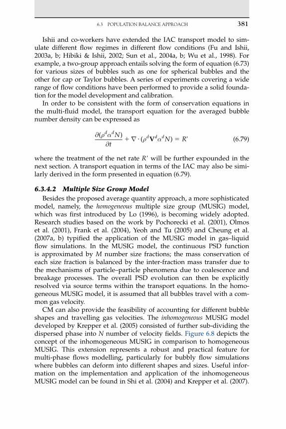
model, namely, the homogeneous multiple size group (MUSIG) model, which was first introduced by Lo (1996), is becoming widely adopted. Research studies based on the work by Pochorecki et al. (2001), Olmos et al. (2001), Frank et al. (2004), Yeoh and Tu (2005) and Cheung et al. (2007a, b) typified the application of the MUSIG model in gas–liquid flow simulations. In the MUSIG model, the continuous PSD function is approximated by M number size fractions; the mass conservation of each size fraction is balanced by the inter-fraction mass transfer due to the mechanisms of particle–particle phenomena due to coalescence and breakage processes. The overall PSD evolution can then be explicitly resolved via source terms within the transport equations. In the homo-geneous MUSIG model, it is assumed that all bubbles travel with a com-mon gas velocity.
CM can also provide the feasibility of accounting for different bubble shapes and travelling gas velocities. The inhomogeneous MUSIG model developed by Krepper et al. (2005) consisted of further sub-dividing the dispersed phase into N number of velocity fields. Figure 6.8 depicts the concept of the inhomogeneous MUSIG in comparison to homogeneous MUSIG. This extension represents a robust and practical feature for multi-phase flows modelling, particularly for bubbly flow simulations where bubbles can deform into different shapes and sizes. Useful infor-mation on the implementation and application of the inhomogeneous MUSIG model can be found in Shi et al. (2004) and Krepper et al. (2007).

6. Gas–LiquidFLows382
In spite of the sacrifices being made to computational efficiency, the extra computational effort will rapidly diminish due to foreseeable advance-ment of computer technology; the CM should therefore suffice as the pre-ferred approach in tackling more complex multi-phase flows.
The formulation of the MUSIG model originates from the discretized PSE which is given by
∂∂
∇Nt
N Riid
i i ( )V
(6.80)
Similar to DQMOM, equation (6.78) can also be written in a form con-sistent with the variables used in multi-fluid model. In terms of size frac-tion, the transport equation becomes
∂∂
∇ ( )( ) i
d di
id
id d
i if
tf R V
(6.81)
For the homogeneous MUSIG model, equation (6.80) reduces to the form where all poly-dispersed phases are assumed to travel with a com-mon velocity Vd. Hence,
∂∂
∇( )
d d
i d d di i
ft
f R ( )V
(6.82)
For the inhomogeneous MUSIG model, equation (6.80) can nonetheless be re-expressed in terms of the size fraction of the ith bubble size class, where i[1, Mj], and velocity group j, where j[1, N], according to
∂
∂∇ ( )
( ) j
djd
ijd
jd
jd
i i
f
tf R V
(6.83)
VdJ Vd
J VdJ
Vd
Bubble breakage Bubble coalescence
Homogeneous MUSIG
Inhomogeneous MUSIG
d1 dm1dm1+1 dm1+m2
FIgure 6.8 An illustration of the MUSIG model.

6.4 bubbLEintEraCtionMECHanisMs 383
with additional relations and constraints given by
d
jd
j
N
ijd
i
M
j
N
jd
id
i
M
ii
Mj j j
f 1 11 1 1
1∑ ∑∑ ∑ ∑, ,
(6.84)
The net rates of Ri in equation (6.82) and R in equation (6.83) will be
treated in the next section.It should be noted that Snayal et al. (2005) have examined and com-
pared the CM and QMOM in a two-dimensional bubbly column simula-tion. Both methods yielded very similar results. The CM solution has been found to be independent of the resolution of the internal coordinate if a sufficient number of classes were adopted. Computationally, as the num-ber of transport equations depends on the number of groups adopted, the MUSIG model requires more computational time and resources than the MOM to achieve stable and accurate numerical predictions.
6.4 BuBBle InteractIon MechanISMS
The IAC represents the key parameter that links the interaction between the phases. In gas–liquid flows, considerable attention has been concentrated towards describing the temporal and spatial evolution of the two-phase geometrical structure caused by the effects of coalescence and break-up through the interactions among bubbles as well as between bubbles and turbulent eddies in turbulent flows. In view of this, the major phenomenological mechanisms have been identified and appro-priate mechanistic models have subsequently been established. In bubbly flow conditions, they include
l coalescence through random collision driven by turbulent eddies;l coalescence due to the acceleration of the following bubble in the
wake of the preceding bubble;l break-up due to the impact of turbulent eddies.
The schematic illustrations of these mechanisms are shown in Figure 6.9. Final expressions for the particle number source or sink terms due to such mechanisms for either the single average scalar or multiple bubble size approach are presented in the following sections.
6.4.1 Single average Scalar approach for Bubbly Flows
As shown in equation (6.78), the term R in the right-hand side of the equation must be specified by the constitutive relations. The population balance of dispersed bubbles in bubbly flow conditions is governed by

6. Gas–LiquidFLows384
the three mechanisms of bubble coalescence and break-up of which the term can be written as
R d d
NRC
NTI
NWE φ φ φ( )
(6.85)
where φNRC, φN
TI and φNWE are the bubble number density changes due to
random collision, turbulent-induced breakage and wake entrainment. With the assumption of spherical bubbles, the transport equation of the averaged bubble number density is equivalent to the transport equation of the IAC.
6.4.1.1 Wu et al. (1998) ModelAn empirical modelling of the bubble coalescence and bubble break-
age that has been widely cited is the model developed by Wu et al. (1998). Considering the characteristic times for binary collision and the
Coalescence mechanisms
Break-up mechanisms
Bounce
Merge
Random collision
Turbulent impact
Unaffected
Uneven breakage due to fluid shearing
Even breakage
Wake entrainment
FIgure 6.9 Major bubble interaction mechanisms in bubbly flow conditions.

6.4 bubbLEintEraCtionMECHanisMs 385
mean travelling length between neighbouring bubbles, they have mod-elled the random collision rate of bubble coalescence according to
φ
e N
RCRC
d d
sdC
D
C
( ) ( )( )
2 1 3
11 3 1 3 1 3 1 3 1/
/max
/max
/ /( )exp
max/ /
max/ /
1 3 1 3
1 3 1 3
( )( )
d
d
(6.86)
where CRC 0.021 and C 3.0 are adjustable model constants representing the coalescence efficiency. The maximum allowable void fraction max takes the value of 0.8, which considers the point of transition from slug to annu-lar flow. Assuming a spherical bubble travelling with its terminal velocity, the rate of collision caused by wake entrainment is however expressed as
φ
NWE
WE r
d
s
C UD
( )2
4
(6.87)
where CWE 0.0073 is a model constant determining the effective wake length and the coalescence efficiency. The terminal velocity of bubbles, Ur, is given by
U
D gCrs
D
c d
c3
( ) −
(6.88)
Turbulent-induced break-up is derived from a simple momentum bal-ance approach. In this mechanism, Wu et al. (1998) restricted only eddies with the same size as the bubbles responsible for breakage. The rate of bubble break-up is given by
φ
eNTI
TI
d d
s
cr crCD
WeWe
WeWe
( ) /
/
1 3
11 3 1 exp
(6.89)
From the above expression, CTI 0.0945 and the critical Weber num-ber Wecr 2.0, which governs the criterion of breakage, are adjustable parameters.
6.4.1.2 Hibiki and Ishii (2002) ModelSome experimental observations (Otake et al., 1997; Serizawa &
Kataoka, 1988) have argued that the coalescence due to wake entrain-ment is only significant between pairs of large cap bubbles (slug flow regime) in fluid sufficiently viscous to maintain their wake laminar; whereas small spherical or ellipsoidal bubbles tend to repel each other. In contrast to the model of Wu et al. (1998), Hibiki and Ishii (2002) have ignored the wake entrainment coalescence due to its insignificant event in bubbly flow condition.

6. Gas–LiquidFLows386
By assuming that the bubble movement behaves analogously to ideal gas molecules, the coalescence rate due to turbulent random collision can be determined as
φ
e
eNRC
RC
d d
sd
c dsC
DC
D= −
−−
( ) ( )( )
exp( ) ( )/
/max
/ /2 1 3
11 3
1 2 1 3 5//
/
6
1 2
(6.90)
Instead of using the constant in the Wu et al. (1998) model, the coales-cence efficiency is derived from the liquid-film-thinning model (Oolman & Blanch, 1986a, b) and dimensional consideration for turbulent flow (Levich, 1962) using the Coulaloglou and Tavlarides (1977) expression as the main framework. The constants CRC 0.03 and C 1.29 are adjust-able model constants that have been calibrated through experiments.
Hibiki and Ishii (2000a) have also derived the breakage rate from kinetic theory. The breakage rate is correlated to the frequency for a given bubble colliding with the turbulent eddy as
φ
e
eN
TITI
d d d
sd c dC
DC
D= −
−−
−( ) ( )( )
( )exp
( )
/
/max
/
2 1 3
11 3 2 31
ss5 3/
(6.91)
In the above expression, CTI 0.03 and C 1.37 are adjustable model constants that have been determined experimentally.
6.4.1.3 Yao and Morel (2004) ModelYao and Morel (2004) have pointed out that the aforementioned two
models have been developed based on two different considerations: the free travelling time or the interaction time. They argued that both char-acteristic times are identically important. Taking two considerations into account, the bubble coalescence rate is derived as
φ
e N
RCRC
d d
s
RC crdC
D
C We We
1
2 1 3
11 32
1 3( ) ( ) exp( / )
( )
/
/max
/ − / max1 3
3/ / C We WeRC
dcr
(6.92)
where the derived constants are CRC1 2.86, CRC2 1.017 and CRC3 1.922, respectively. Similarly to the Hibiki and Ishii (2002) model, coalescence caused by wake entrainment is neglected.
For bubble break-up, they disputed that bubble breakage is mainly caused by the resonance oscillation. Considering the natural frequency of the oscillating bubbles, the interaction time can be approximated and the rate of bubble breakage is given by
φ
eN
TId d d
s
crdD
We We
We W=
− −
+ −1 6
11 0 42 1
1 3
11 3.( )( ) exp( / )
. ( ) /
/
/ eecr (6.93)
6.4 bubbLEintEraCtionMECHanisMs 387
where the constants are CTI1 1.6 and CTI2 0.42. The critical Weber number of 1.42 is employed (Sevik & Park, 1973). Considering the transi-tion point from the finely dispersed bubbly flow to slug flow, the maxi-mum allowable void fraction in Hibiki and Ishii (2002) and Yao and Morel (2004) models retains a value of 0.52.
6.4.2 Multiple Bubble Size approach for Bubbly Flows
Suitable constitutive relations must be appropriately specified in the right-hand side of equations (6.68), (6.82) and (6.83) of which phenome-nological models developed particularly by Prince and Blanch (1990) and Luo and Svendsen (1996) can be employed to describe the mechanisms of coalescence and break-up of intermittent bubbles.
For the merging of bubbles, the coalescence of two bubbles is assumed to occur in three stages. The first stage involves the bubbles colliding, thereby trapping a small amount of liquid between them. This liquid film then drains until it reaches a critical thickness. The last stage features the rupturing of the liquid film subsequently causing the bubbles to coalesce. The collisions between bubbles may be caused by turbulence, buoyancy and laminar shear. Only random collisions driven by turbulence are usu-ally considered for bubbly flow conditions. The coalescence kernel con-sidering turbulent collision taken from Prince and Blanch (1990) can be written as the product of the collision rate and coalescence efficiency:
a M M a M M P d di j ij C i j( ) ( ) ( ), , ,
(6.94)
where the collision rate can be expressed as the product of the collision cross-sectional area A and characteristic velocity u as
πij i j
A
ti tj
u
d d u u
42 2 1 2[ ]( )
(6.95)
while the coalescence efficiency is
P d dt
C i jij
ij( ), exp
(6.96)
The contact time ij when two bubbles come together is
eijij
c
d
( )
( )
/ /
/
2 2 3
1 3
(6.97)

6. Gas–LiquidFLows388
while the time required for two bubbles to coalesce tij can be estimated to be
td h
hij
cij
f
( )/ln
2
16
3 1 2
0
(6.98)
In equation (6.97), the equivalent diameter dij is calculated as sug-gested by Chesters and Hoffman (1982):
dd dij
i j
2 21
(6.99)
where the diameters di and dj are evaluated based on the spherical bubble assumption as
d M d Mi d i j d j
6 1 6 11 3 1 3
π π
,
(6.100)
For air–water systems, experiments have determined h0, initial film thickness and, hf, critical film thickness at which rupture occurs to be 1 104 and 1 108 m, respectively. The turbulent velocity ut in the inertial sub-range of isotropic turbulence by Rotta (1972) is given by
u dtc 1 4 1 2 1 3. ( )e (6.101)
Similar to the Hibiki and Ishii (2002) and Yao and Morel (2004) mod-els, coalescence caused by wake entrainment is normally neglected for bubbly flow conditions.
For the consideration of the breakage of bubbles, the model developed by Luo and Svendsen (1996) is employed for the break-up of bubbles in turbulent dispersions. In this model, binary break-up of the bubbles is assumed and the model is based on surface energy criterion and isotropic turbulence. The break-up frequency for binary break-up of bubbles is
r M M r M M Cd
i jd
c
i
( ) ( ) ( )( )
, ,min
11
2
1 3 2
11 3e
11
2 3 5 3 11 3
12
∫
exp
c
ddf
c ci
e
( )
(6.102)

6.4 bubbLEintEraCtionMECHanisMs 389
where /dj is the size ratio between an eddy and a particle in the inertial sub-range and consequently min min/dmin. The lower limit of the integration is given by
d Mdmin min min, .
6 111 4
1 3
π
(6.103)
in which υ e (( ) )c c3 1 4/ / , where vc denotes the kinematic viscosity of the continuous phase. The constants C and are determined, respec-tively, from fundamental consideration of drops or bubbles breakage in turbulent dispersion systems to be 0.923 and 2.0. The variable cf denotes the increase coefficient of surface area:
c f ff BV BV [ ]2 3 2 31 1( )
(6.104)
where fBV is the breakage fraction: Mj/Mi. On the basis of the definition of the break-up kernel defined in equation (6.102), the terms (M) and p(M, M) can be written as
b M M
Mr M M dM
M
( )( )
( )
, ,1
0
∫
(6.105)
p M Mr M M
r M M dMM
( )( )
( )
,,
,
0
∫
(6.106)
6.4.2.1 DQMOM ModelFor DQMOM, the moment transform of the coalescence and break-up
of the term Sk can be expressed as
S B D B Dk kC
kC
kB
kB (6.107)
where
B U M a U M f M t f U t dUdMk
C k 12
00
( ) ( ) ( ) ( ), , ,∞∞
∫∫
(6.108a)
D M a M M f M t f M t dM dMk
C k ( ) ( ) ( ), , ,00
∞∞
∫∫
(6.108b)
6. Gas–LiquidFLows390
B M M b M M p M M f M t dM dMk
B k ( ) ( ) ( ) ( ), , ,00
∞∞
∫∫
(6.108c)
D M b M M f M t dMk
B k
0
∞
∫ ( ) ( ), ,
(6.108d)
where the terms B and D represent the birth and death rates of the coales-cence and break-up of bubbles. In equation (6.108a), note that the term has been derived by using U M M and substituting dM dU. On the basis of the approximation given in equation (6.60), the birth and death rates can be written as
P N N M M a M Mk
Ci j i j
ki j
ji
12
( ) ( ),∑∑
(6.109a)
D M a M M N Nk
Cik
i j i jji
( ),∑∑
(6.109b)
P M r M M Nk
Bik
j i jji
( ),∑∑
(6.109c)
D M r M M Nk
Bik
i j iji
( ),∑∑
(6.109d)
From above, the weights Ni and Nj can be determined according to the definition given in equation (6.71). Coalescence and break-up kernels defined in equations (6.94) and (6.100) can be employed to evaluate the above birth and death rates.
6.4.2.2 MUSIG ModelThe treatment of the net source or sink term Ri
in equation (6.82) and Ri
in equation (6.83) is described in the following. Source or sink rates due to coalescence and break-up are also those of birth and death rates as expressed in equation (6.103) for the DQMOM model. In other words,
R R B D B Di i iC
iC
iB
iB (6.110)
On the basis of the discrete approximation given in equation (6.74), the birth and death rates can be formulated according to
B M N N a M Mi
Ci k l k l
lk
12
( ),∑∑
(6.111a)

6.4 bubbLEintEraCtionMECHanisMs 391
D M N N a M Mi
Ci i k i k
k
( ),∑
(6.111b)
B M r M M Ni
Bi k i j
k
( ),∑
(6.111c)
D M N r M Mi
Bi i i k
k
( ),∑
(6.111d)
In order to be consistent with equations (6.82) and (6.83), the above birth and death rates are required to be expressed in terms of the size fraction. For the homogeneous model, they can be written as
B f f
M MM M
a M MiC d d
k lk l
k lk l
lk
( ) ( ) 2 12
,∑∑
(6.112a)
D f f
Ma M Mi
C d di k
ki k
k
( ) ( ) 2 1,∑
(6.112b)
B r M M fi
B d dk i j
k
( ),∑
(6.112c)
D f r M Mi
B d di i k
k
( ),∑
(6.112d)
while for the inhomogeneous model, they are
B f f
M MM M
a M MiC
jd
jd
k lk l
k lk l
lk
( ) , 2 12
( )∑∑
(6.113a)
D f f
Ma M Mi
Cjd
jd
i kk
i kk
( ) , 2 1( )∑
(6.113b)
B r M M fi
Bjd
jd
k i kk
( ),∑
(6.113c)
D f r M Mi
Bjd
jd
i i kk
( ),∑
(6.113d)
For the discretized contribution of the birth rate due to coalescence, it may be necessary to introduce the coalescence mass matrix as the fraction

6. Gas–LiquidFLows392
of mass due to coalescence between the kth bubble classes which goes into the ith bubble classes. Defining the coalescence mass matrix as
kli
k l iM M M
10,,
if otherwise
the birth rate due to coalescence is accordingly modified by multiplying the above matrix kli into equations (6.112a) and (6.113a), respectively. Similar to the DQMOM model, coalescence and break-up kernels defined in equations (6.94) and (6.100) can also be employed to evaluate the above birth and death rates for the homogeneous and inhomogeneous models accordingly.
6.4.3 comments of other coalescence and Break-up Kernels
With respect to the coalescence kernels, several other expressions have been proposed in addition to the model by Prince and Blanch (1990). Based on the same collision rate consideration as stipulated in equa-tion (6.95), Chesters (1991) has proposed an alternate expression for the coalescence efficiency which can be written as
P d d c
WeC i j( ), exp
/
2
1 2
(6.114)
where We is the Weber number defined by
We
dc cij
e
( )2 3 5 3
2
/ /
(6.115)
in which the equivalent diameter dij is evaluated according to equation (6.99). Another rather complex expression for the coalescence efficiency is the proposal by Luo (1993) which takes the form
P d d cC i jij ij
d c( )( / )
, exp[ . ( )( )]
. (
/
/
0 75 1 1
0 5 1
2 3 1 2
1 2
iijij ij
i
jWe
dd3
1 2
),/
(6.116)
in which We u dijc
ij i 2 / and u u u dij i jc
i ij ( ) ( )/ / /2 2 1 2 1 2 2 31( )e , where is set equal to 2.0. In both equations (6.114) and (6.116), the con-stant c is prescribed a value of 0.4. Lehr et al. (2002), however, have pro-posed different expressions not only to the coalescence efficiency but also for the characteristic velocity in the collision rate. In addition to the con-sideration of the turbulent velocity in the inertial sub-range of isotropic turbulence, the characteristic velocity also accounts for the difference

6.4 bubbLEintEraCtionMECHanisMs 393
in rise velocities of the bubbles. The characteristic velocity can now be expressed as
u d d U Uc
i j T i T j max . , , ,1 4 1 3 2 3 2 3( )e( )
(6.117)
where UT,i UT,j represents the relative velocity between the bubbles which can be determined from their respective terminal velocities. For a bubble diameter greater than 1.3 mm, the terminal velocities may be eval-uated as suggested by Clift et al. (1978):
Ud
gd Ud
gdT i ci
i T j cj
j, ,.
. ,.
. 2 14
0 5052 14
0 505
(6.118)
The expression for the coalescence efficiency can be written as
P d duuC i jcrit
d
d( ), max , exp max
11 3
1
2
(6.119)
where the critical velocity ucrit and the maximum packing maxd are set
to values of 0.08 m/s and 0.6, respectively. It should be noted that the above coalescence efficiency models as well as the model by Prince and Blanch (1990) are based on phenomenological analysis and they provide probability functions that are employed to modify the collision frequency models in order to determine the appropriate coalescence rates. These are thus very strongly influenced by the hydrodynamic conditions and the interfacial characteristics of the flow system.
Concerning break-up kernels, other phenomenological models have also been proposed besides the model by Luo and Svendsen (1996). Lehr et al. (2002) have derived an expression in which capillary pressure con-straint is incorporated and the interfacial and inertial forces are assumed to balance each other. These additional constraints favour the formation of larger break-up fractions, thus avoiding the evolution of infinitely small daughter bubbles. The break-up kernel for binary breakage of bubbles is
r M Md f
i j ci
cBV fBV
( )( )
( ), .
exp
/ / / //
1 191
16 3 1 3 1 3
2
13 3
1
1 3
e
∫
2
2 3 5 3 2 3 1 3
e c c
i BVd fd
( ) / / / /
(6.120)
Another model for the bubble break-up kernel proposed by Martínez-Bazán et al. (1999a) considered the balance between the turbulent stress

6. Gas–LiquidFLows394
and surface tension force. According to their model, the expression is given by
b M K
d d
dc
i g
ci
ci
i( )
( )e
e ,
/( )/
2 3 12
(6.121)
where the constant 8.2 has been ascertained from Batchelor (1956) and Kg 0.25 was found experimentally by Martínez-Bazán et al. (1999a).
On the basis of the model by Luo and Svendsen (1996), it predicts the bubble undergoing breakage into a given combination of daughter bub-ble sizes that is defined by a U-shaped daughter bubble probability dis-tribution function. On the other hand, the model by Martínez-Bazán et al. (1999b) predicts that the break-up process is described by an inverted U-shaped (I-shaped) daughter bubble probability distribution function. The prediction of the daughter bubble probability distribution function for lower breakage rates by the model of Lehr et al. (2002) yields maximum probability for equivalent-size breakage but an M-shaped daughter bub-ble probability distribution function with two peaks close to zero break-age void fractions as the break-up rate increases. Size distribution of the daughter bubbles through this model is thus a function of the size ratio of given bubbles to that of the maximum stable bubble size where larger bubbles are more likely to break into unequal daughter bubbles, whereas small bubbles are more likely to break into equal size daughter bubbles.
6.4.4 Modelling Beyond Bubbly Flows – a Phenomenological consideration
In bubbly flows, the transport phenomena of dispersed bubbles can be regarded in a similar view of the drag and interaction mechanisms of spherical bubbles. As the gas velocity increases, experimental obser-vations have nonetheless clearly shown the prevalence of cap bubbles of which these bubbles are normally precursors to the formation of slug units in the slug flow regime such as shown for two-phase flow in a ver-tical pipe in Figure 6.2. At even higher gas velocities, large unsteady gas volumes will begin to accumulate within these mixing motions and pro-duce the churn-turbulent flow regime with increasing volume fractions. In order to model the interfacial transport phenomena of fluid particles in all two-phase flow regimes, it is rather sensible and makes perfect sense that the effects due to the differences in bubble size and shape should be carefully considered. The modelling framework includes the classifica-tion of bubbles of different sizes and shapes into different groups, which entails now the consideration of additional transport equations to aptly describe the transport phenomena of these distinct groups of bubbles

6.4 bubbLEintEraCtionMECHanisMs 395
such as has been proposed by Ishii et al. (2002). Such a model presents great potential since it possesses the capability of accounting for the wide spectrum of bubble sizes that may exist in different flow regimes. The PBE can be written in a general form as
∂∂
∇Nt
N S Si di birth death ( )V
(6.122)
where Ni is the individual bubble number density representing discrete bubble classes and Vd the averaged bubble velocity weighted by the gas void fraction. The right-hand side of equation (6.122) presents the birth and death terms due to coalescence and break-up of bubbles.
A schematic representation for the multi-group multi-bubble-class model is illustrated in Figure 6.10. For each bubble shape, a set of dis-crete bubble-class equations in the form presented in equation (6.122) can be solved. With reference to Figure 6.10, a two-group multi-bubble-class model accommodates the consideration of intra-group interactions for the spherical and cap/slug bubbles. Essentially, two sets of PBEs are solved for each intra-group. In other words,
∂∂
∇N
tN Si
sphericald spherical
ispherical
birthspherical
( ),V Sdeathspherical
(6.123)
∂∂
∇N
tN S Si
capd cap
icap
birthcap
deathcap
( ),V
(6.124)
Spherical
d1,d2,...,dn d1,d2,...,dn d1,d2,...,dn
Discretebubble classresolution forsphericalbubble
Discretebubble classresolution forcap bubble
Discretebubble classresolution forother bubbleshape
Inter-group interactions
Cap Other
FIgure 6.10 An illustration of the multi-group multi-bubble-class model.

6. Gas–LiquidFLows396
The possible interactions of the two-group bubbles that are accounted for through the source and sink terms in equations (6.123) and (6.124) are illustrated in Figure 6.11. As shown in Figure 6.12, the probable mecha-nisms of these interactions can be distinguished in five categories:
l coalescence due to random collisions driven by liquid turbulence;l coalescence due to wake entrainment;l break-up due to the impact of turbulent eddies;l shearing-off of small bubbles from cap/slug bubbles;l break-up of large cap bubbles due to flow instability on the bubble
surface.
For the intra-group mechanisms for spherical bubbles, the usual coalescence and break-up processes due to random collisions and tur-bulent impact that have been extensively described in previous sections can be adopted. The intra-group mechanisms for cap/slug bubbles take however a more complex consideration where the bubble coalescence is due to random collisions and wake entrainment, while the bubble break-up is attributed to turbulent impact, shearing-off and surface instability.
Group 1(1+1 and 1)
Group 2(2+2 and 2)
Inter-group(1+2 and 2)
Coalescence Break-up
Inter-group(1+1 and 2)
FIgure 6.11 Classification of possible interactions of two-group bubbles (after Hibiki & Ishii, 2009).

6.4 bubbLEintEraCtionMECHanisMs 397
With reference to Figure 6.12, the wake entrainment for cap/slug bubbles predominantly governs the cap/slug bubble number which significantly affects the flow structure and intensiveness of inter-group interactions such as depicted in Figure 6.11. Here, when bubbles enter the criti-cal wake region of a preceding bubble, they can accelerate and coalesce with this preceding bubble according to the mechanisms based upon the critical distance of a probability approach such as proposed by Sun et al. (2004a, b). Nevertheless, the cap/slug bubble disintegration due to surface instability can be significantly enhanced by the high turbulent intensity and active eddy–bubble interaction in the wake region of the slug bubbles. This occurs when the volume of the resulting bubble from bubble coalescence exceeds the maximum bubble stable limit; it becomes unstable and disintegrates. The mechanism for the shearing-off effect is reflected by the fact that the bubbles shearing-off from the cap/slug bubbles contribute as a primary source for the spherical bubbles and ulti-mately the IAC. More details on the mechanisms for cap/slug bubbles can be found in Hibiki and Ishii (2000a, b), Fu and Ishii (2003a, b) and Sun et al. (2004a, b).
In addition to the intra-group interactions, it has been demonstrated through experiments performed by Hibiki and Ishii (2000a, b) that the inter-group interactions also contribute significantly to the transport of the interfa-cial states. Similar mechanisms from the above considerations for intra-group interactions may be derived accordingly for the inter-group interactions.
Coalescence mechanisms
Break-up mechanisms
Random collision Wake entrainment
Turbulent impact Shearing-off Surface instability
FIgure 6.12 Schematic illustrations of the mechanisms associated with the two-group bubble interactions (after Hibiki & Ishii, 2009).

6. Gas–LiquidFLows398
6.5 ModellIng SuB-cooled BoIlIng FlowS
Modelling low-pressure sub-cooled boiling flow in the context of com-putational fluid dynamics can be broadly classified according to two categories: (a) heat transfer and the consideration of wall heat flux par-titioning during sub-cooled boiling flow at the heated wall and (b) two-phase flow and bubble behaviours in the bulk sub-cooled flow away from the heated wall. The presence of a heated wall represents the fun-damental difference between isothermal bubbly and sub-cooled boiling flows, where the former has a constant bubble injection rate to govern the overall void fraction of the gas phase, but the latter has a variable bubble nucleation rate which is subjected predominantly by the heat-transfer and phase-changing phenomena.
6.5.1 review of current Model applications
The mechanistic model by Kurul and Podowski (1990), adapted by Judd and Hwang (1976) on the premise of a model for wall heat flux partitioning during pool nucleate boiling, is the model most widely employed in many computational fluid dynamics investigations of sub-cooled boiling flows at low pressures. The fundamental idea of the model is to assume all the energy from the wall is transferred to the liquid adja-cent to the heated wall. Thereafter, a fraction of the energy is transferred to the vapour bubbles by evaporation while the remainder goes into the bulk liquid. In essence, the model entails the partitioning of the wall heat flux into three heat flux components. They are: (a) heat transferred by conduction to the superheated layer next to the wall (nucleate boiling or surface quenching) Qq, (b) heat transferred by evaporation or vapour generation Qe and (c) heat transferred by turbulent convection Qc. The wall heat flux partitioning can be written as
Q Q Q Qw q e c
(6.125)
Firstly, the surface quenching heat flux is determined through the relationship:
Q C f A T Tq
c cpc
q wc
2π
( )
(6.126)
where Tw is the wall temperature and T c the continuous-fluid tempera-ture adjacent to the heated surface. Secondly, the heat flux due to vapour

6.5 ModELLinGsub-CooLEdboiLinGFLows 399
generation at the wall in the nucleate boiling region can be simply calcu-lated from Bowring (1962):
Q N f d he a bw
gfg
π
63
(6.127)
Thirdly, the heat flux according to the definition of local Stanton num-ber St for turbulent convection is
Q St C u T T Ac
cpc c
wc
q ( )( )1
(6.128)
where uc is the local tangential fluid velocity of the continuous phase adjacent to the heated surface. The evaluation of the area of the heater surface influenced by bubbles Aq is given by
A K
dNq
bwa
π 2
4 (6.129)
where the empirical constant K is used to account for the area of the heater surface influenced by the bubble. A value of K 4 is often rec-ommended (Kurul & Podowski, 1990). However, Kenning and Del Valle (1981) have found values ranging between 2 and 5. Judd and Hwang (1976) ascertained that a lower value, K 1.8, best fitted their experimen-tal data.
In order to determine each respective component on the right-hand side of equation (6.125), a bisection algorithm, an iterative procedure, is normally employed to evaluate the wall superheat that satisfies the applied wall heat flux. This algorithm begins with a guess of the wall superheat, and thereafter calculates each component of the heat flux. The difference between the computed total wall heat flux and the actual applied wall heat flux provides a new wall superheat estimate for the next step in iterative procedure. The iteration continues until the differ-ence error between the applied and calculated wall heat flux falls below a prescribed criterion (i.e. 104) of the applied heat flux.
Suitable relationships are required for the bubble departure diameter dbw, frequency f and active nucleation site density Na that appear in the wall heat flux partition model, which can be closed through the prescrip-tion of appropriate correlations.
A number of studies examining bubble growth and detachment have resulted in a number of different empirical correlations for bubble depar-ture. We focus on the selected relationships that are relevant to low-pressure sub-cooled boiling flow. Tolubinsky and Kostanchuk (1970)

6. Gas–LiquidFLows400
proposed a simple relationship which evaluated the bubble departure as a function of the sub-cooling temperature Tsub as
d
Tbw
sub min . exp , .0 000645
0 00014
(6.130)
On the basis of the balance between the buoyancy and surface tension forces at the heating surface, Fritz (1935) proposed a correlation which includes the contact angle of the bubble:
d
gbw c d
0 0208.
( )
(6.131)
where is the contact angle. The above expression was modified by Kocamustafaogullari and Ishii (1995) for low pressure as
d
gbw
c d
d c d
2 5 10 5.
( )
(6.132)
A more comprehensive correlation proposed by Unal (1976) which included not only the effect of sub-cooling but also the convection veloc-ity and heater wall properties is given by
d
p a
bbw 2 42 10 5 0 709. .
Φ (6.133)
where
aQ hT
C h C
C
Cb
Tw subc
fgc c
pc d
w w pwc c
pc
su
( )1 3
1 32
/
/ ( / ),
π
bbd c2 1[ / ] ( )
Ch C h Pr
g
ufg l p
cfg
c d
c
( )
( )
;0 013
0 61
1 7 3.
.
.
Φ
0 47
0 61
1 0 0 61
.
.
. .
for m/s
for m/s
u
u
c
c
The stated range for this correlation is
Pressure MPaWall heat flux MW/mLiq
: . .: . .
0 1 17 70 47 10 64 2< << <
pQw
uuid velocity m/sLiquid sub-cooling C
: . .: .
0 08 9 153 0
< <<u
Tc
sub << 86°C

6.5 ModELLinGsub-CooLEdboiLinGFLows 401
For the bubble departure frequency, most correlations have been derived from the consideration of the bubble departure diameter. Cole’s correlation (1960), which was derived assuming a balance between buoy-ancy and drag (drag coefficient constant) for pool nucleate boiling, is a popular expression, which is given by
fd
gbw
c d
c0 5 4
3.
( )
(6.134)
In the hydrodynamic region, Ivey (1967) has suggested a bubble fre-quency relationship, which can be used for coalesced bubbles. The cor-relation is simply
fd gbw0 5 0 9. .
(6.135)
A slightly more complicated expression by Stephan (1992), which included the effect of surface tension, may also be employed for the low-pressure sub-cooled boiling flow. It is given as
fd
gd
gdbw bw c
bw
1
24
π
(6.136)
Similar expressions of the bubble frequency correlation that include the surface tension effect in the form of equation (6.136) are also noted. Peebels and Garber (1953) observed the velocity rise in a gravitational field as
V
gb
c d
c
1 18 2
0 25
..
( )
( )
(6.137)
On the basis of equation (6.132), Jakob (1949) proposed a bubble fre-quency by assuming the waiting time to be equivalent to the growth time, thus resulting in
fdg
bw
c d
c
0 59 2
0 25
..
( )
( )
(6.138)
The Lemmert and Chwala’s (1977) active nucleation site density relationship is commonly used in the wall heat flux partitioning model which has been correlated based on Del Valle and Kenning (1985) data. It can be determined simply from the local wall superheat as
N m T Ta w satn [ ]( ) (6.139)

6. Gas–LiquidFLows402
According to Kurul and Podowski (1990) the values of m and n are 210 and 1.805, respectively. Recently, Koncar et al. (2004) demonstrated that better predictions were obtained by reducing the value of m to 185. Kocamustafaogullari and Ishii (1995) correlated existing active nucleation site density data by means of parametric study. They have assumed the active nucleation site density in pool boiling by both surface conditions and thermo-physical properties of the fluid. They also postulated that the active nucleation site density developed for pool boiling could be used in a forced convective system by the use of an effective superheat rather than the actual wall superheat. The active nucleation site density, Na, can be expressed as
Nd
T
T hfa
bw
sat
effc
fg
1 22
4 4
∆
.
*( )
(6.140)
where * (c d)/d and the function f(*) is a known function of a density ratio described by
f ( ) *) ( ) * . ( . *. . 2 157 10 1 0 00497 3 2 4 13 (6.141)
In equation (6.140), Teff represents the effective superheat, which is given by Teff S Tw, where Tw Tsat Tw and S is the suppression factor. Basu et al. (2002) proposed an alternative empirical correlation that included the effect of contact angle on the active nucleation site density, which is given by
N T T T K
Na w ONB w
a
0 34 10 1 15
3 4 10 1
4 2 0
1
. cos
. cos
.( )
( )
∆ ∆ ∆
∆TT K Tw w5 3 15. ∆ (6.142)
Hibiki and Ishii (2003) modelled the active nucleation site density rela-tionship mechanistically by the knowledge of the size and cone angle distributions of cavities. In accordance with Basu et al. (2002) correlation, they have also formulated the nucleation site density as a function of contact angle. The correlation is given by
Na 4 72 10 14 17
2 5 152
. exp.
exp .
00
216 f
T h
Tw
cfg
sat( )
∆
(6.143)
where the function f() is a function described by
f ( ) . . ( . ) ( . ) 0 01064 0 48246 0 22712 0 054682 3 (6.144)
with log10((c d)/d).
6.5 ModELLinGsub-CooLEdboiLinGFLows 403
Within the bulk sub-cooled flow, Anglart and Nylund (1996) have proposed the bubble Sauter diameter to be modelled as a function of the local water sub-cooling Tsub from the following equation:
D
D d T TD T T D T T
s
B sub sub
B sub sub B sub sub
1 1 1
1 2 2 1
for ( ) ( )
(
,
, ,
TT TT T T
D d T Tsub sub
sub sub sub
B sub sub
, ,, ,
,
1 22 1
2 2 2
)for
for
(6.145)
Alternatively, a more sophisticated expression proposed by Zeitoun and Shoukri (1996a, b) could be employed to evaluate the bubble Sauter diameter instead of the linear functional expression of equation (6.145), which is given by
D
g Re Jasc d
c d
subc d
/
. /( (( . /
.
.( )
( )(
0 0683149 2
1 326
0 324 ))1 326 0 487 1 6. . .)/( )))Bo Re
(6.146)
where Re is the flow Reynolds number, Bo the boiling number and Jasub the Jakob number based on the liquid sub-cooling.
6.5.2 Phenomenological description
As observed in Lee et al. (2002) and Tu et al. (2005), high-speed pho-tography in the vicinity of the heated wall, as shown in Figure 6.13, clearly confirms the presence of large bubbles away from the heated wall. More importantly, the bottom vapour bubble at upstream can be seen to be sliding along the heated surface before being impeded by the down-stream bubble (see Figure 6.13). Such observation has also been con-firmed by experiments performed by Bonjour and Lallemand (2001) and Prodanovic et al. (2002), which clearly indicated the presence of bubbles sliding shortly after being detached from the heated cervices before lift-ing into the bulk sub-cooled liquid core. In their experiments, they have also seen that these upstream bubbles travelling closely to the heated wall have the tendency to collide with any detached bubbles downstream, and subsequently form bigger bubbles due to bubble merging or coales-cence of adjacent bubbles. The supposition of larger bubbles being pres-ent due to bubble coalescence was evident away from the heated wall, as shown in Figure 6.14. Focusing on the local bubble mushroom region, as depicted in Figure 6.14, and tracking its development through time, the region increased in size along the heated wall downstream, confirm-ing the significant coalescence of bubbles. On the other hand, very few

6. Gas–LiquidFLows404
bubbles were present in the bulk sub-cooled liquid further away from the heated wall and near the unheated wall. In this flow region, the effect of condensation gradually caused the bubbles to decrease in size due to the sub-cooling temperature of the liquid as they migrated towards the opposite end of the unheated wall of the flow channel. This was further confirmed by experimental observations of Gopinath et al. (2002) (see Figure 6.15), which illustrated a bubble gradually being condensed in a sub-cooled liquid away from the heated surface.
On the basis of the above experimental observations, it is clear that bubbles in an upwards sub-cooled boiling flow have a tendency to slide before lifting off into the bulk sub-cooled liquid. In such a case where the bubbles may merge with other nucleating bubbles while sliding, a
0 s 1.96 X 10⁻³s 3.92 X 10⁻³s 5.89 X 10⁻³s
FIgure 6.13 Bubble sliding behaviour and collision with downstream bubble near the heated wall of an annular flow channel (Lee et al., 2002).
0 ms 12 ms 24 ms 36 ms
FIgure 6.14 Significant bubble coalescence near the heated wall of an annular flow channel as indicated by the increasing bubble mushroom region (Tu et al., 2005).

6.5 ModELLinGsub-CooLEdboiLinGFLows 405
smaller number of bubbles will be lifted off from the heated surface area than the actual number of active nucleation sites. The transient conduc-tion due to sliding bubbles becomes the dominant mode of heat transfer. It is therefore imperative that the wall heat partition model incorporates the heat-transfer component due to these sliding bubbles. It has also been established through our investigations in Yeoh et al. (2002) that empirical correlations such as those exemplified in equations (6.145) and (6.146) can at best only provide a macroscopic description of the boiling phenom-enon. Not surprisingly, these relationships are unable to adequately rep-resent some important complex mechanistic behaviours of bubbles such as bubble coalescence and condensation (microscopic in nature) that have been observed in experiments. To account for these bubble behaviours, the sub-cooled boiling model must be further developed with the consider-ation of population balance approach with the inclusion of the nucleation and condensation processes. The improved wall heat partition model and homogeneous MUSIG boiling model are described in the next sections.
t = 0.0 ms t = 0.8 ms t = 1.6 ms
t = 2.4 ms t = 3.2 ms t = 4.0 ms
t = 4.8 ms t = 5.6 ms t = 6.4 ms
FIgure 6.15 Bubble undergoing condensation in the bulk sub-cooled liquid (Tu et al., 2005).

6. Gas–LiquidFLows406
6.5.3 nucleation of Bubbles at heated walls
Enhancement in heat transfer during forced convective boiling can be attributed by the presence of both sliding and stationary bubbles. There are essentially two mechanisms: (a) latent heat transfer due to micro-layer evaporation and (b) transient conduction as the disrupted thermal boundary-layer reforms during the waiting period (i.e. incipience of the next bubble at the same nucleation site).
Transient conduction occurs in regions at the point of inception and in regions being swept by sliding bubbles. For a stationary bubble, the heat flux Qtc is given by
QC
tT T R N K
Dt f
C
tc
c cpc
ww
cf a
dw
c cpc
24
2
2
ππ
π
( )
ttT T R N
Dt f
ww
cf a
dw( ) ( )
π 2
41
(6.147)
where Dd is the bubble departure diameter and tw the waiting time. Equation (6.147) indicates that some fraction of the nucleation sites will undergo transient conduction, while the remaining will be in the growth period. For a sliding bubble, the heat flux Qtcsl due to transient conduc-tion that takes place during the sliding phase and the area occupied by the sliding bubble at any instant of time is given by
QC
tT T R N l KD t f
C
tT T R N
tcsl
c cpc
ww
cf a s a w
c cpc
ww
cf
2
2
π
π
( )
( ) aa sla
wftD
t fπ 2
41
( )
(6.148)
where the average bubble diameter Da is given by Da (Dd Dl)/2 and Dl is the bubble lift-off diameter. Strictly speaking, the Kurul and Podowski’s model is only applicable for sub-cooled boiling flows where bubbles are immediately released into the bulk sub-cooled liquid, hence the absence of the bubble sliding phenomenon. This may be possibly true for pool boiling flows in a horizontal orientation.
The reduction factor Rf appearing in equations (6.147) and (6.148) depicts the ratio of the actual number of bubbles lifting off per unit area of the heater surface to the number of active nucleation sites per unit area, viz., Rf 1/(ls/s), where ls is the sliding distance and s the spacing between nucleation sites. In the present study, it shall be assumed that the nucleation sites are distributed in a square grid and that the bubbles slide only in the direction of the fluid flow (Brackbill et al., 1992). The spacing

6.5 ModELLinGsub-CooLEdboiLinGFLows 407
between nucleation sites can thus be approximated as s Na 1/ , where Na can be evaluated based upon the correlation of Koncar et al. (2004): Na [210(Tw Tsat)]1.805. The factor Rf is obtained alongside with the sliding distance evaluated from the force balance model (to be described below). The significance of this factor provides information whereby the bubble departing from its site of origin merges with other nucleating bubbles at adjacent sites. It is noted that for the case where the sliding distance ls is less than the spacing s, Rf 1.
Forced convection will always prevail at all times in areas of the heater surface that are not influenced by the stationary and sliding bubbles. The fraction of the heater area for stationary and sliding bubbles is given by
1 14 4
12 2
A R N KD
t f ND
tq f ad
w adπ π
( ww
a s w a sl w
f
N l KDt f N ftD
t f
)
( )
π 2
41
(6.149)
Numerous studies have attempted to tie the bubble departure fre-quency to some other parameter, namely the departing bubble diameter. Although the relationship between the bubble departure frequency and departing bubble diameter offers an attractive means of determining the frequency, application of these relationships, predominantly correlated from pool boiling data, remains contentious for forced convective boil-ing flow. For example, Cole’s bubble frequency relationship (equation (6.134)) is frequently employed in many investigations of sub-cooled boiling flows. In order to eliminate the uncertainty of evaluating the bubble frequency, it is proposed that the fundamental theory based on the description of an ebullition cycle in nucleate boiling, which are: (1) waiting period tw (transient conduction of heat to liquid) and (2) growth period tg: (a) bubble growth rate, (b) evaporation process, (c) agitation of liquid around the bubble and (d) termination of bubble whether by departure or collapse, is employed instead. In other words,
f
t tg w
1
(6.150)
In order to remove the application uncertainty of correlations empiri-cally determined for the departing bubble diameter, a force balance model is developed. The model concentrates on the various forces that influence the growth of a bubble during flow conditions in the directions paral-lel and normal to a vertical heating surface. These forces are formulated

6. Gas–LiquidFLows408
according to the studies performed by Klausner et al. (1993) and Zeng et al. (1993). Figure 6.16 illustrates the forces acting on the bubble in the x-direction and y-direction; they are, respectively,
F F F F F Fx sx dux sL h cp∑
(6.151)
dFx
Fy
Fsx
Fsy
α
β
θ
g
x
y
dw
U(x)
Heatedwall
Fb
Slidingdistance
l s
Bubble growth
Departure
Sliding
Lift off
i
FIgure 6.16 Schematic illustrations of the forces acting on a growing vapour bubble and bubble departing, sliding and lifting off from a vertical surface.

6.5 ModELLinGsub-CooLEdboiLinGFLows 409
and
F F F F Fy sy duy qs b∑
(6.152)
where Fs is the surface tension force, Fdu the unsteady drag due to asym-metrical growth of the bubble and the dynamic effect of the unsteady liq-uid such as the history force and the added mass force, FsL the shear lift force, Fh the force due to the hydrodynamic pressure, Fcp the contact pres-sure force accounting for the bubble being in contact with a solid rather than being surrounded by liquid, Fqs the quasi-steady drag in the flow direction and Fb the buoyancy force. In addition, g indicates the gravita-tional acceleration, , and i are the advancing, receding and inclina-tion angles, respectively, dw the surface/bubble contact diameter and d the vapour bubble diameter at the wall.
The forces acting in the x-direction can be estimated from
F d F Fsx w dux du i
π
[cos cos ], cos
F C U r F U
dF
drsL L
ch
c wcp
w
r
12
94 4 4
22 2 22 2
π π π
∆ ∆, ,
In the y-direction, they are
F d F Fsy w duy du i
π π
( )
( )2 2 [sin sin ], sin
F C U r F r gqs D
cb
c d 643
3 π π ∆ , ( )
From the various forces described along the x-direction and y-direction, r is the bubble radius, U the relative velocity between the bubble centre of mass and liquid, CD and CL the respective drag and shear lift coeffi-cients and rr the curvature radius of the bubble at the reference point on the surface x 0, which is rr 5r (Klausner et al., 1993).
The drag coefficient CD and shear lift coefficient CL appearing in the drag and lift forces are determined according to the relationships pro-posed by Klausner et al. (1993). In other words,
CReD
b
nn
n
23
120 796
1
.
/
(6.153)

6. Gas–LiquidFLows410
C G
ReGL s
bs 3 877
10 0141 2
22
1 4
. .//
(6.154)
where n 0.65 and Reb c Ud/c is the bubble Reynolds number. The dimensionless shear rate Gs is (dU/dx)(r/U). The gradient dU/dx can be determined through the universal velocity profile for turbulent flow:
Uu
x
2 5 9 8. ln .( )
(6.155)
where u is the friction velocity and x lux/l the non-dimensional nor-mal distance from the heated wall. In equation (6.155), the velocity profile is assumed to be applicable for the time-averaged velocity distribution in the vicinity of the heated wall. Adjacent velocities, determined through the two-fluid model, are used to obtain the varying local friction velocities through equation (6.155). These friction velocities are subsequently used to evaluate the gradients dU/dx along the heated wall to determine the shear rate Gs.
The growth force Fdu is modelled by considering a hemispherical bub-ble expanding in an inviscid liquid, which is given by Zeng et al. (1993) as
F r C r rrdu
cs π 2 23
2
(6.156)
where (·) indicates differentiation with respect to time. The constant Cs is taken to be 20/3 according to Zeng et al. (1993). In estimating the growth force, additional information on the bubble growth rate is required. Also in Zeng et al. (1993), a diffusion-controlled bubble growth solution by Zuber (1961) is adopted:
r t
bJa t Ja
C T
h C
cpc
wd
fg
c
cpc( )
2π
, ,∆
(6.157)
where Ja is the Jakob number, the liquid thermal diffusivity and b an empirical constant that is intended to account for the asphericity of the bubble. For the range of heat fluxes investigated in this investigation, b is taken to be 0.21 based on a similar sub-cooled boiling study performed by Steiner et al. (2005), which has been experimentally verified through their in-house measurements with water as the working fluid.
While a vapour bubble remains attached to the heated wall, the sum of the parallel and normal forces must satisfy the following conditions: ΣFx 0 and ΣFy 0. For a sliding bubble case, the former establishes the bubble departure diameter (Dd), while the latter yields the bubble lift-off diame-ter (Dl). The growth period tg appearing in equation (6.150) can be readily

6.5 ModELLinGsub-CooLEdboiLinGFLows 411
evaluated based on the availability of the bubble size at departure from its nucleation site through equation (6.158). The lift-off period tl can also be similarly calculated based on the bubble lift-off diameter. The differ-ence between the bubble lift-off and bubble growth periods provides the period for the sliding bubble; the sliding distance ls can subsequently be determined (see Figure 6.16). An estimation on this sliding distance can be determined according to the experimental correlation of Maity (2000) as l C ts v sl ( / )2 3 3 2/ , where tsl is the sliding time (tl tg) and Cv an acceleration coefficient correlated in terms of the tangential liquid velocity (ul) adjacent to the heated surface: Cv 3.2ul 1. This coefficient reflects the increase in bubble velocity with time after it begins to slide away from a nucleation site.
The bubble waiting time tw is determined through the occurrence of transient conduction when a bubble slides or lifts off, of which the boundary layer gets disrupted and cold liquid comes in contact with the heated wall. Assuming that the heat capacity of the heater wall wCpww is very small, the conduction process can be modelled by considering one-dimensional transient heat conduction into a semi-infinite medium with the liquid at a temperature T c and the heater surface at a temperature Tw. The wall heat flux can be approximated by
Q
T Tw
cw
c
c
( )
(6.158)
where πc )(= t is the thickness of the thermal boundary layer. If the temperature profile inside this layer is taken to be linear according to Hsu and Graham (1976), it can thus be expressed as
T T
T T xb s
wc
c ( )
(6.159)
where Ts is the temperature of the heater. In equation (6.159), x represents the normal distance from the wall. Based on the criterion of the incipi-ence of boiling from a bubble site inside the thermal boundary layer, the bubble internal temperature for a nucleus site (cavity) with radius rc is
T T
T
C r hx C rb sat
sat
c fgd c
2
21
, at
(6.160)
where C1 (1 cos )/sin and C2 1/sin . The angle referred to here represents the bubble contact angle as described previously. By substituting equation (6.160) into equation (6.159), the waiting time tw can be obtained as
t tT T C r
T T C h rw
wc
c
w satd
fg c
12
1
2
2
π ( )
∆ /
(6.161)

6. Gas–LiquidFLows412
The cavity radius rc can be determined by applying Hsu’s criteria and tangency condition of equations (6.83) and (6.84):
tC C h r
TT T
QT
dfg c
sat
wc c
w
w
1 2
2 22 2
2
π
( ) ( Tc )2
π
(6.162)
From equation (6.162),
r FT
h Qc
satc
dfg w
2
1 2
/
(6.163)
where
F
C C
111 2
1 2 2 1 2
/ /sin
cos
(6.164)
According to Basu et al. (2002), the factor F indicates the degree of flooding of the available cavity size and the wettability of the surface. If the contact angle → 0, all the cavities will be flooded. Alternatively, as → 90°, F → 1, all the cavities will not be flooded (i.e. they contain traces of gas or vapour).
In reality, the surface/bubble contact diameter dw evolves from the point of inception until the point of departure or lift off. Here, a correla-tion based on the experimental data of Maity (2000) as a function of the bubble contact angle is employed to determine the ratio of the bubble base diameter dw to the bubble diameter at departure or lift off, which is given as C 1 exp(20.6). Experimental observations by Klausner et al. (1993) and Bibeau and Salcudean (1994) have indicated that the advancing angle and receding angle varied quite substantially during the sliding phase. Considering the complexity of the bubble departure and bubble lift off, and the difficulty in obtaining the measurements, the advancing and receding angles can be reasonably evaluated through the bubble contact angle as and . Klausner et al. (1993) have employed an angle of 4.5° in their theoretical analysis, whereas Bibeau and Salcudean (1994) have reported a value of 2.5°. According to Winterton (1984), the angle has nonetheless been postulated to be as high as 10°. In the present study, an angle of 5° is adopted. For the inclination angle i, a value of 10° that gave the best fit to the data by Klausner et al. (1993) is employed for the current force balance model.

6.5 ModELLinGsub-CooLEdboiLinGFLows 413
6.5.4 condensation of Bubbles in Sub-cooled liquid
For the homogeneous MUSIG model, the transport equation govern-ing the conservation of mass for the vapour phase takes the same form of equation (6.82) as
∂∂
∇( )
( )
d d
i d d di i
ft
f R V
(6.165)
where the source or sink term Ri is given by
R S M Ri i i ph i
( ) (6.166)
In equation (6.166), the first term Si represents the source or sink term due to coalescence and break-up rates, which is effectively given by equations (6.106) and (6.112a)–(6.112d). The second term (Rph)i essentially comprises of the formulation of the source or sink rate for the phase-change processes associated with sub-cooled boiling flow. The bubble sink rate due to con-densation in a control volume for each bubble class can be determined from
φCOND
i
BB
BNV
AdRdt
(6.167)
The following holds for the bubble condensation velocity (Domilovskii et al., 1979):
dRdt
h T T
hB sat
c
dfg
( )
(6.168)
Substituting equation (6.168) into equation (6.167) and given that the bubble surface area AB and volume VB based on the Sauter bubble diameter are, respectively, πDs
2 and πDs3 6/ , equation (6.167) can be
re-arranged as
( )( )
RD
h T Thph i COND d d
d
s
satc
fg
φ
1 6
Nha T T
hNi d d
if satc
fgi
l
1
( )
Γ
(6.169)
where Γl represents the mass-transfer rate due to condensation in the bulk sub-cooled liquid in which h represents the inter-phase heat-transfer coefficient determined from Ranz and Marshall (1952) Nusselt number correlation and aif is the interfacial area between phases per unit volume.

6. Gas–LiquidFLows414
At the heated surface, bubbles form at activated cavities known as active nucleation sites. Since the bubble nucleation process only occurs at the heated surface, this heated wall nucleation rate is not included in (Rph)i but rather specified as a boundary condition to the vapour phase transport equation (6.165) apportioned to the discrete bubble class based on the bubble departure criteria on the heated surface. The wall vapour generation rate is modelled in a mechanistic way derived by considering the total mass of bubbles detaching from the heated surface as
Γ
g e
fg pc
sub
Q
h C T
(6.170)
where Qe is the heat transfer due to evaporation which is given by equation (6.127). The gas void fraction along with the scalar fraction fi is related to the number density of the discrete bubble ith class Ni (similarly to the jth class Nj) as gfi NiVi, where V is the volume of the bubble. The size distri-bution of the vapour or dispersed phase is therefore defined by the scalar fi.
6.6 worKed exaMPleS
Specific modelling approaches and techniques in the context of computational fluid dynamics to resolve isothermal and sub-cooled boiling bubbly flows using the two-fluid formulation based on the inter- penetrating media framework are discussed via relevant worked examples described below. All numerical results presented have been computed through the use of the commercial computer codes of ANSYS, Inc., CFX. For sub-cooled boiling flows, however, they have been obtained through the older version of CFX4.4.
6.6.1 dispersed Bubbly Flow in a rectangular column
Computed results that are presented in this worked example are based on the numerical simulations performed by Krepper et al. (2007). This study centres on a rectangular bubble column having a width of 0.1 m, a depth of 0.02 m and a height of 1.0 m. Figure 6.17 shows a schematic drawing of the three-dimensional column geometry. The bubble column is operated in the dispersed bubbly flow regime, which is characterized by the absence of bubble coalescence or break-up. According to the bubble column rectangular map of Lin et al. (1996), the gas plume breaks up into bubbles of 3–5 mm in size. During experiments as evidenced in Krepper et al. (2007), images obtained from a high-speed camera are employed to observe the general pattern and they are processed to calculate the bubble velocities, bubble-turbulence parameters and bubble size distributions.

6.6 workEdExaMpLEs 415
Gas disengagement technique is used to attain the volume-averaged gas fraction over a range of superficial gas velocities. The local void fraction at two different height positions is measured via the mesh sensor in which the data provide the necessary means of comparing against the model predictions. The purpose of this example is to demonstrate the impor-tance of non-drag forces affecting the isothermal bubbly flow.
6.6.1.1 Numerical FeaturesThe phenomenon of an aerated bubble column is a transient process. An
unsteady two-fluid model is applied to solve two sets of equations gov-erning the conservation of mass and momentum. In the actual experiment, the flow is isothermal; only the momentum interfacial exchange must
Inflow of gas bubbles
0.02 m
0.01 m
0.1 m
1.0 m
Measuring plane atheight of 0.08 m
Measuring plane atheight of 0.63 m
Outflow
FIgure 6.17 Schematic drawing of the three-dimensional bubble column geometry.

6. Gas–LiquidFLows416
therefore be considered in this worked example. The advection term is discretized using a second-order scheme weighted between central and upwind differencing, whereas the diffusion time is approximated accord-ing to the second-order central differencing (CD) scheme. For the time derivative term, it is approximated via a second-order backwards Euler time discretization scheme. The liquid turbulence is modelled according to the SST model of Menter (1993), which switches between the standard k–e model (for the flow away from the column walls) and k– turbulence model (for the flow vicinity of column walls) using a blending function. Sato et al.’s (1981) eddy-viscosity model for bubble-induced turbulence is applied to accommodate the influence of the gas bubbles on the liq-uid turbulence. A coupled solver is adopted for the momentum and pres-sure equations which are then solved iteratively with the turbulent scalar equations in an implicit manner for each time step.
For the modelling of momentum interfacial exchange, the drag force is calculated according to equations (6.14) and (6.15). The drag coeffi-cient CD is nonetheless determined through the correlation of Grace et al. (1976) in the distorted regime instead of the Ishii and Zuber (1979) corre-lation, which can be written in the form:
C
gD
UD
c d
cs
T
4
3 2
(6.171)
where the terminal velocity UT is given by
U
DM JT
c
cs
0 149 0 857. .( )
(6.172)
From equation (6.172), J is determined through
J
H HH H
0 94 2 59 33 42 59 3
0 751
0 441. .. .
.
.
(6.173)
in which H can be expressed in terms of the Eotvos number defined in equation (6.23) and Morton number defined as
M
g c c d
c( ) ( )
( )
4
2 3
(6.174)
by
H EoM
c
ref
43
0 1490 14
..
(6.175)

6.6 workEdExaMpLEs 417
where ref is the molecular viscosity normally set for water at some refer-ence temperature and pressure.
In addition to the drag force, the so-called non-drag forces acting per-pendicular to the flow direction are also incorporated into the momen-tum equation, namely, the lift, turbulent dispersion and wall lubrication forces. Firstly, a positive lift force acts in the direction of decreasing liq-uid velocity. For the case of co-current upwards flow, it is in the direc-tion towards the column wall. A negative lift force acts away from the column wall especially for bubbles with large deformations. Herein, the lift coefficient force is determined through the expression given in equa-tion (6.25) with the lift coefficient evaluated based on the correlations of Tomiyama (1998) such as expressed in equation (6.26) in order to account for positive and negative lift forces. Secondly, the wall lubrication force represents a wall force which pushes the gas bubbles away from the wall. It takes the form suggested by Antal et al. (1991) as expressed in equation (6.28) except that the wall constant Cw is now modelled as
C C
D
y D yw w
s
w ww
3
2
2 221 1
( )
n
(6.176)
where D is the diameter of the flow channel and the constant Cw3 is eval-uated based on the correlation of Tomiyama (1998):
C
Eo EoEo Eo 33w30 933 0 179 1 5
0 007 0 04 5
exp . .. .
( ){ (6.177)
Thirdly, the turbulent dispersion force is a result of the turbulent fluc-tuations of the liquid velocity. The force derived by Gosman et al. (1992) is applied which is of a similar expression as stipulated in equation (6.31) obtained through Burns et al. (2004) and based upon Favre-averaged drag modelling.
On the basis of bubble size distributions measured through the wire-mesh sensor in Figure 6.18, the averaged bubble size and the width of bubble distributions increase with increasing superficial gas velocities (jgas). For superficial gas velocity less than 10 mm/s, the maximum bub-ble size found is smaller than the critical bubble diameter of 5.8 mm. For the mono-dispersed approach considered in this study, an averaged bub-ble size of Ds 3 mm is assumed. With reference to the measured and calculated final gas volume fractions for different superficial gas veloci-ties in Figure 6.19, the good agreement that is achieved between the mea-sured and calculated values justifies the application of a constant bubble size for the numerical calculations.
The rectangular bubble column is simulated using a regular hexagonal mesh having a grid spacing of 5 mm. Grid independence is checked by

6. Gas–LiquidFLows418
investigating three different mesh densities on the predictions of final gas volume fractions. Table 6.1 presents the numerical results for the super-ficial gas velocity of 0.01 m/s. In comparison to the reference mesh, the prediction of the final gas volume fractions does not appreciably change
0.6
0.4
0.2
jgas = 2 mm/s
00 5 10
0.6
0.4
0.2
jgas = 4 mm/s
00 5 10
0.6
0.4
0.2
jgas = 10 mm/s
00 5
Bubble size (mm)
∆ε/
∆D
bub
(%/m
m)
Bubble size (mm)10
0.6
0.4
0.2
jgas = 20mm/s
00 5 10
0.6
0.4
0.2
jgas = 6 mm/s
00 5 10
0.6
0.4
0.2
jgas = 8 mm/s
00 5 10
FIgure 6.18 Bubble size distributions measured by the wire-mesh sensor.
0 5 10 15 20 25
0.0
0.05
0.1
0.15
jgas (mm/s)
Ave
rage
d ga
s vo
lum
e fr
actio
n
Experiment
Prediction
FIgure 6.19 Measured and calculated final gas volume fractions.

6.6 workEdExaMpLEs 419
even when the mesh is doubled in the depth – mesh A, doubled in the width – mesh B and doubled in all three directions – mesh C. Table 6.2 shows the calculated final gas volume fractions for different time steps. Here, a time step of 0.005 s indicates the appropriate selection of time step to perform the transient calculations.
6.6.1.2 Numerical ResultsDuring the experiment, the bubbly flow within the rectangular channel
reveals two distinctive flow behaviours. Just above the gas injection point, oscillating plumes are seen such as described by the experimental obser-vations in Figure 6.20. This plume-like structure subsequently disappears beyond a certain height. Approximately after an axial distance of 1.5–5 times the width of the column, depending on the superficial gas velocities, the bubbles are found to rise in a string-like motion with a non-oscillating flow. The model prediction also yields similar qualitative behaviour such as those seen from the transient snapshot of the gas volume frac-tion distribution after a problem time of 30 s for superficial gas velocity of 10 mm/s with the consideration of drag and non-drag forces in Figure 6.21. To investigate the influence of the non-drag forces, a series of calcu-lations are performed without the consideration of these forces. Figure 6.22 exemplifies a transient snapshot of the gas volume fraction distribu-tion after a problem time of 30 s for the case where only the drag force is
taBle 6.1 differentMeshdensitiesontheGasVolumeFractionforsuperficialGasVelocityjgas0.01m/s
Mesh Nodes (W D H) Number of cellsFinal gas volume
fraction
Reference case 20 4 200 16,000 0.0426
A 20 8 200 32,000 0.0408
B 40 8 200 64,000 0.0405
C 40 8 400 128,000 0.0405
taBle 6.2 differenttimestepsontheGasVolumeFractionforjgas0.01m/s
Time stepFinal gas volume
fraction
Reference case – 0.005 s 0.0426
0.0025 s 0.0416
0.01 s 0.0427

6. Gas–LiquidFLows420
considered (left side). The solution of a meandering oscillating flow behaviour persists throughout the bubble column. Based on this solu-tion, the influence of the various non-drag forces is parametrically inves-tigated. From the same figure (right side), the lift force is seen to be the force that exerts the largest dominance, wherein the gas volume fraction
t = t0 t = t0 + 0.75 s t = t0 + 1.5 s t = t0 + 2.25 s t = t0 + 3.5 s
FIgure 6.20 Experimental observations of plume oscillations at superficial gas velo-city jgas 4 mm/s.
0.15
0.1125
0.075
0.0375
0.0
Gas volume fractionNon-oscillation
region
Oscillationregion
FIgure 6.21 Two distinctive regions observed during experiment (left side) and a snapshot of calculated gas volume fraction after a problem time of 30 s for superficial gas velocity jgas 10 mm/s (right side).

6.6 workEdExaMpLEs 421
distribution, the largest gradient of the gas volume fraction, is found. This means that the lift force has an equalizing damping effect of the flow behaviour especially away from the gas injection point. For the other two forces, the turbulent dispersion force is only significant near the gas injec-tion, while the wall lubrication force yields considerable influence near the wall.
Figure 6.23 shows the comparison between the measured calculated lateral gas volume fraction distributions at the measuring planes of 0.08 m (near the gas injection) and 0.63 m (upper region of bubble col-umn), respectively. Averaging of the numerical results is performed over a time period when the averaged gas volume fraction has reached a steady value. The experimental values are determined by time averaging of the local gas volume fractions measured by the wire-mesh sensor. For the values in the upper region, good agreement is achieved between the measurements and calculations, especially in the calculated maxima near the right and left walls. Nevertheless, the two-fluid model with its cur-rent configuration is not able to resolve the turbulence structures of the oscillating gas plumes near the gas injection. This flow behaviour could be possibly resolved through the consideration of large eddy simulation.
0.15
0.1125
0.075
0.0375
0.0
Gas volume fraction
100.0
75.0
50.0
25.0
0.0
Force (N)
Drag Lift Turbulentdissipation
Walllubrication
FIgure 6.22 Calculated gas volume fraction with only drag force (left side) and based on this solution calculated magnitude of the different components of non-drag forces.

6. Gas–LiquidFLows422
0 0.02 0.04 0.06 0.08 0.1
0.0
0.025
0.05
0.075
Axial distance (m)
Gas
vol
ume
frac
tion
Experiment Prediction
jgas = 10 mm/s
jgas = 8 mm/s
jgas = 6 mm/s
Height = 0.63 m
0 0.02 0.04 0.06 0.08 0.1
Axial distance (m)
jgas = 10 mm/s
jgas = 8 mm/s
jgas = 6 mm/s
0.0
0.025
0.05
0.075
Gas
vol
ume
frac
tion
Experiment Prediction
Height = 0.08 m
FIgure 6.23 Time-averaged spatial gas volume fraction distributions at height of 0.63 m (upper region) and height of 0.08 m (near gas injection).
6.6 workEdExaMpLEs 423
6.6.1.3 ConclusionIn this worked example, a mono-dispersed approach with an assumed
bubble size has been shown to adequately predict the two-phase bubbly flow behaviour within the rectangular column geometry. The simulation of the transient flow pattern is found to be strongly influenced by the modelling of non-drag forces. Without the non-drag forces, the numeri-cal simulations show a meandering oscillation of the gas volume frac-tion distribution throughout the whole domain, due to which the flow can be stabilized via the effect of the lift force. Although good agreement between measurements and calculations can be achieved in the upper region, the two-fluid model formulation fails to aptly resolve the turbu-lent structures of prevailing oscillating gas plumes, especially near the gas injection point which requires a more elaborate model.
6.6.2 Bubbly Flow in a Vertical Pipe
Two population balance approaches based on the one-group average bubble number density model and MUSIG model for predicting the bub-ble size distribution of gas–liquid bubbly flows under isothermal condi-tions are demonstrated in this worked example. Experimental data of isothermal gas–liquid bubbly flow in a vertical pipe performed by Liu and Bankoff (1993a, b) and Hibiki et al. (2001) are utilized to appropri-ately assess the relative merits of both approaches in the context of com-putational fluid dynamics framework.
A schematic diagram of the experimental set-up of Liu and Bankoff (1993a, b) is shown in Figure 6.24. The test section is a 2800 mm long, vertical acrylic pipe with an internal diameter D 38 mm. Bubbles are produced and injected into the test section at the bottom. Local radial measurements are obtained at the axial location z/D 36.0. Liquid velocity is attained by using hot-film anemometers, while local void frac-tion and gas velocity are measured by a two-point resistivity probe. A total of 48 flow conditions covering the range of superficial gas velocities (0.0270.347 m/s) and superficial liquid velocities (0.3761.391 m/s) are investigated. The bubble diameters are controlled in a narrow range of 2–4 mm during the whole course of the experiments.
Similar to the set-up of Liu and Bankoff (1993a), a separate isothermal air–water flow experiment conducted by Hibiki et al. (2001) comprises of an acrylic round pipe test section with an inner diameter D 50.8 mm and a length of 3061 mm. Local flow measurements using the double sen-sor and hot-film anemometer probes are carried out at three axial (height) locations of z/D 6.0, 30.3 and 53.5 and 15 radial locations of r/R 0–0.95. Experiments are performed for a range of superficial liquid and gas velocities, which cover most of the bubbly flow regions including finely dispersed bubbly flow and bubbly-to-slug transition flow regions.

6. Gas–LiquidFLows424
The primary aim in this worked example is to compare the two popu-lation balance approaches for simulating the bubbly flow regime. Six flow conditions are investigated as depicted in Figure 6.25. Also included in the figure, the solid lines represented the different flow regime transition boundaries predicted by the model of Taitel et al. (1980). As shown in the figure, all six flow conditions lie within the bubbly flow region. Details of the flow conditions are summarized in Table 6.3. For ease of discussion, experiments by Liu and Bankoff (1993a) and Hibiki et al. (2001) are here-after referred to as Exp. 1 and Exp. 2, respectively.
6.6.2.1 Numerical FeaturesIn modelling isothermal gas–liquid bubbly flow, the two-fluid model
which is based on solving two sets of equations governing the conser-vation of mass and momentum is adopted. The advection term is dis-cretized using a second-order scheme weighted between central and
38.0 mm
Test channel inletwith bubble injected
50.8 mm
z/D = 30.3
Test channel inletwith bubble injected
z/D = 6.0
z/D = 53.5
z/D = 36.0(a) (b)2800 mm 3061 mm
FIgure 6.24 Schematic drawing of the experimental test sections: (a) Liu and Bankoff (1993a) and (b) Hibiki et al. (2001).

6.6 workEdExaMpLEs 425
Superficial gas velocity, ⟨jg⟩ (m/s)
Sup
erfic
ial l
iqui
d ve
loci
ty, ⟨
j f⟩ (m
/s)
10–2 10–1 100 101
10–1
100
101
Taitel et al.Exp. 1Exp. 2
Transition condition
Bubbly flow Slug flow
Finely dispersed bubbly flow
FIgure 6.25 Map of flow regime and the bubbly flow conditions studied in this worked example.
taBle 6.3 bubblyFlowandinletboundaryConditions
Superficial liquid velocity, ⟨ ⟩jf (m/s)
Superficial gas velocity, ⟨ ⟩jg (m/s)
Bubbly flow regime Transition regime
Liu and Bankoff (1993a) experiment
1.087 0.0270 0.1120
[g z D/ .0 0 (%)] [2.5] [10.0]
[DS z D/ .0 0 (mm)] [3.0] [3.0]
Hibiki et al. (2001) experiment
0.491 0.0275 0.0556 0.129
[g z D/ .0 0 (%)] [5.0] [10.0] [20.0]
[DS z D/ .0 0 (mm)] [2.5] [2.5] [2.5]
0.986 0.0473 0.1130 0.242
[g z D/ .0 0 (%)] [5.0] [10.0] [20.0]
[DS z D/ .0 0 (mm)] [2.5] [2.5] [2.5]

6. Gas–LiquidFLows426
upwind differencing, while the diffusion time is approximated according to the second-order CD scheme. For the time derivative term, it is approx-imated via a second-order backwards Euler time discretization scheme. In handling bubble-induced turbulent flow, unlike the single-phase fluid flow problem, no standard turbulence model is tailored for two-phase (gas–liquid) flow. Nevertheless, numerical investigation has revealed that the standard k–e model tends to predict an unrealistically high gas void fraction peak close to the wall (Cheung et al., 2007a; Frank et al., 2004). The SST model by Menter (1993) has been shown to provide a more real-istic prediction of gas volume fraction or void fraction close to the wall. The SST model is thereby employed herein. For all flow conditions, reli-able convergence are achieved within 2500 iterations when the root mean square (rms) pressure residual drops below 1.0 107. A fixed physical time scale of 0.002 s is employed for all steady-state simulations.
As demonstrated from the previous worked example, interfacial momentum exchange in isothermal bubbly flows exhibits a dominant effect in affecting the two-phase flow behaviour. The interfacial forces considered are due to drag, lift, lubrication and turbulent dispersion forces. Firstly, the drag force resulting from shear and form drag is modelled accord-ing to Ishii and Zuber (1979) in which the drag coefficient CD is evaluated based upon the correlation of several distinct Reynolds number regions. Secondly, bubbles rising in a liquid that is subjected to a lateral lift force are correlated to the relative velocity and the local liquid vorticity. For the lift coefficient, CL, the Eotvos number-dependent correlation proposed by Tomiyama (1998) is adopted. Thirdly, the wall lubrication force, which is due to surface tension, is adopted to prevent bubbles from attaching on the solid walls, thereby resulting in a low gas void fraction at the vicinity of the wall area. Modelled according to Antal et al. (1991), the model constants of Cwl 0.0064 and Cw2 0.016 are utilized. Fourthly, the turbulent dis-persion force expression in terms of Favre-averaged variables proposed by Burns et al. (2004) is employed. By default, the turbulent dispersion coeffi-cient CTD 1 and the turbulent Schmidt number t,g 0.9 are adopted.
For the average bubble number density model, three forms of coales-cence and break-up mechanisms by Wu et al. (1998), Hibiki and Ishii (2002) and Yao and Morel (2004) are employed, whereas for the MUSIG model, the coalescence and break-up mechanisms by Prince and Blanch (1990) and Luo and Svendsen (1996) are adopted. The average bubble number density transport equation with appropriate sink or source terms describing the coalescence and break-up rates of bubble is imple-mented within the CFX code. The in-built MUSIG model is applied for the MUSIG simulations. In the present study, bubbles ranging from 0 to 10 mm diameter are equally divided into 10 size groups (see Table 6.4).
Numerical simulations are performed on a 60° radial sector of the pipe with symmetry boundary conditions at both vertical sides. At the inlet of
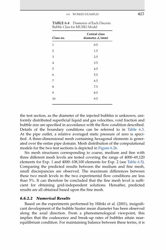
6.6 workEdExaMpLEs 427
the test section, as the diameter of the injected bubbles is unknown, uni-formly distributed superficial liquid and gas velocities, void fraction and bubble size are specified in accordance with the flow condition described. Details of the boundary conditions can be referred to in Table 6.3. At the pipe outlet, a relative averaged static pressure of zero is speci-fied. A three-dimensional mesh containing hexagonal elements is gener-ated over the entire pipe domain. Mesh distribution of the computational models for the two test sections is depicted in Figure 6.26.
Six mesh structures corresponding to coarse, medium and fine with three different mesh levels are tested covering the range of 4000–69,120 elements for Exp. 1 and 4000–108,100 elements for Exp. 2 (see Table 6.5). Comparing the predicted results between the medium and fine mesh, small discrepancies are observed. The maximum differences between these two mesh levels in the two experimental flow conditions are less than 5%. It can therefore be concluded that the fine mesh level is suffi-cient for obtaining grid-independent solutions. Hereafter, predicted results are all obtained based upon the fine mesh.
6.6.2.2 Numerical ResultsBased on the experiments performed by Hibiki et al. (2001), insignifi-
cant development of the bubble Sauter mean diameter has been observed along the axial direction. From a phenomenological viewpoint, this implies that the coalescence and break-up rates of bubbles attain near-equilibrium condition. For maintaining balance between these terms, it is
taBle 6.4 diametersofEachdiscretebubbleClassforMusiGModel
Class no.Central class
diameter, di (mm)
1 0.5
2 1.5
3 2.5
4 3.5
5 4.5
6 5.5
7 6.5
8 7.5
9 8.5
10 9.5

6. Gas–LiquidFLows428
imperative that the coalescence rate is reduced by a factor of 1/10 in the average bubble number density model (i.e. φ φ φ φN
TINTI
NRC
NRC and 0 1. ).
Similarly, coalescence and breakage calibration factors (i.e. FC and FB) with values equal to 0.05 and 1.0 are introduced into the coalescence and break-up rates for the MUSIG model. One plausible explanation for
(a)
Symmetry boundary
Symmetry boundary
(b)
Inlet
Inlet
FIgure 6.26 Mesh distribution of computational models: (a) Liu and Bankoff (1993a) and (b) Hibiki et al. (2001).
taBle 6.5 detailsofnumericalMeshesadoptedfortheGridindependencestudy
Liu and Bankoff (1993a) Hibiki et al. (2001)
L W H Total L W H Total
Coarse 10 10 40 4,000 10 10 40 4,000
Medium 20 20 40 16,000 26 26 80 54,080
Fine 24 24 120 69,120 30 30 120 108,000

6.6 workEdExaMpLEs 429
this discrepancy could be attributed by the lack of resolution of the two-equation k–e turbulent model in predicting the turbulence energy dissi-pation under the two-phase flow condition. It should be emphasized that the reduction and calibration factors are introduced herein by the mere means for engineering estimation, which may be case sensitivity and subject to the flow condition. Although adjustment to the reduction and calibration factors could invariably obtain ‘better’ results, it loses, how-ever, the predictive nature of the models and the common ground for comparison. Therefore, values of these factors are fixed for all the cases and flow conditions that are presented below.
Experimental Data of Liu and Bankoff (1993a, b)Figure 6.27 illustrates the void fraction distributions obtained from the
MUSIG model and the three coalescence/breakage mechanisms employed in the average bubble number density model comparing with the mea-sured data at the dimensionless axial position z/D 36.0. From a physi-cal viewpoint, the phase distribution patterns along the radial direction of the bubble column correspond to four basic types of distributions: wall
Radial position (–)(a)
Tim
e av
erag
ed g
as v
oid
frac
tion
(–)
0 0.2 0.4 0.6 0.8 10
0.05
0.1
0.15
0.2
0.25
0.3
0.35
0.4
Exp. 1Wu et al.Hibiki & IshiiYao & MorelMUSIG
Radial position (–)(b)
Tim
e av
erag
ed g
as v
oid
frac
tion
(–)
0 0.2 0.4 0.6 0.8 10
0.05
0.1
0.15
0.2
0.25
0.3
0.35
0.4
Exp. 1Wu et al.Hibiki & IshiiYao & MorelMUSIG
FIgure 6.27 Predicted radial void fraction distribution at z/D 36.0 and experimen-tal data of Liu and Bankoff (1993b).
6. Gas–LiquidFLows430
peak, intermediate peak, core peak and transition, such as categorized by Serizawa and Kataoka (1988).
In the bubbly flow regime, maximum void fraction located close to the wall demonstrates the flow phase distributions typically known as the ‘wall peak’ behaviour, which is mainly due to the positive lift force push-ing the small bubbles towards the pipe wall. As depicted in Figure 6.27, a well-developed wall peaking behaviour is recorded in the experiment and successfully captured by both models. In the case of low gas super-ficial velocity (i.e. [g] 2.5%; see also Figure 6.27(a)), all the coalescence and break-up bubble mechanistic models of the average bubble num-ber density approach underestimate the void fraction at the core of the pipe. In contrast, the MUSIG model provides a closer prediction with the experiment. However, void fractions at the core of the high gas superfi-cial velocity case as shown in Figure 6.27(b) are slightly over-predicted by all models. One possible reason for the over-prediction of the void fraction distribution could be due to the uncertainties associated with the application of the turbulence model, which is unable to adequately predict the appropriate values of turbulent energy dissipation and which subsequently affects the bubbles coalescence/breakage rate.
The measured and predicted radial profiles of the liquid velocity are presented in Figure 6.28. In contrast to single-phase flow, the introduction of bubbles into the liquid flow has the tendency to enhance or reduce the liquid flow turbulence intensity as indicated by Serizawa and Kataoka (1988). In the case of enhanced turbulence, such as depicted in Figure 6.28(b), the liquid velocity profile at the core is flattened by the additional turbulence while having a relatively steep decrease almost mimicking a step change close to the pipe wall. Since the recorded liquid velocity at the wall is not zero, the numerical results expose some uncertainties of the experiment (Politano et al., 2003). Nevertheless, the predicted velocity profiles, particularly the sharp decrease of the decreasing velocities close to the wall, are successfully captured by all models and compared reason-ably well with measurements. The MUSIG model appears to yield mar-ginally better agreement than the other models. This could be attributed to the higher resolution of the bubble size distribution via the MUSIG model. By introducing MUSIG to discretize the range of bubble sizes that could possibly exist within the flow instead of a single average vari-able parameter determined through the average bubble number density approach, the bubble Sauter diameter is seen to be better resolved which leads to enhanced prediction of the liquid velocities.
Experimental Data of Hibiki et al. (2001)Figure 6.29 compares the gas void fraction profiles obtained from the
average bubble number density and MUSIG models with the measured data in four different bubbly flow conditions. For the low void fraction

6.6 workEdExaMpLEs 431
cases, that is, liquid superficial velocity ⟨ ⟩ =j f 0 491. m/s , wall peaking profiles are well established at the first measuring station of z/D 6.0 due to the considerably low liquid and gas velocities. However, the radial void fraction profile subsequently evolves along the axial direc-tion, becoming well-developed void fraction wall peak at the location of z/D 53.5 for liquid superficial velocity ⟨ ⟩ =j f 0 986. m/s . The phenom-enological evolution of the wall peaking behaviours is properly captured by both models.
Local radial gas and liquid velocity distributions at the measuring station of z/D 53.5, close to the outlet of the pipe, are illustrated in Figure 6.30. For the cases of liquid superficial velocity ⟨ ⟩ =j f 0 491. m/s, except for the simulation result exemplified in Figure 6.30(f), the pre-dictions for all the average bubble number density models of the gas and liquid velocity compare favourably with the experimental data. Generally, liquid velocities at the core of the pipe are under-predicted at the location of z/D 53.5 (see also Figure 6.30(f)). Similar observations
Radial position (–)(a)
Tim
e av
erag
ed li
quid
vel
ocity
(m
/s)
0 0.2 0.4 0.6 0.8 10
0.5
1
1.5
2
2.5
Exp. 1
Wu et al.Hibiki & IshiiYao & MorelMUSIG
Radial position (–)(b)
Tim
e av
erag
ed li
quid
vel
ocity
(m
/s)
0 0.2 0.4 0.6 0.8 10
0.5
1
1.5
2
2.5
Exp. 1
Wu et al.Hibiki & IshiiYao & MorelMUSIG
FIgure 6.28 Predicted radial liquid velocity profile at z/D 36.0 and experimental data of Liu and Bankoff (1993a).

6. Gas–LiquidFLows432
are also found for the predictions of the gas or liquid superficial veloc-ity ⟨ ⟩ =j f 0 986. m/s such as those shown in Figure 6.30(c), (d), (g) and (h). Nevertheless, predictions of the MUSIG model as depicted in Figure 6.30(a)–(d) are found to be noticeably better than those of the average bubble number density models. Although the liquid velocities at the core are still under-predicted for liquid superficial velocity ⟨ ⟩ =j f 0 986. m/s , the MUSIG model, in general, still yields better agreement due to the higher resolution of the bubble size distribution which would indi-rectly enhance the liquid velocity predictions by the provision of a more detailed description of the interfacial forces within the interfacial momen-tum transfer between the air and water phases.
Figure 6.31 shows the predicted and measured mean Sauter diameter distributions at two measuring stations, corresponding to that of void
(a)
(e) (f) (g) (h)
(b) (c) (d)Radial position (–)
Tim
e av
erag
ed g
as v
oid
frac
tion
(–)
0 0.2 0.4 0.6 0.8 10
0.05
0.1
0.15
0.2
0.25
0.3
0.35
0.4
Exp. 2
Wu et al.
Hibiki & Ishii
Yao & Morel
MUSIG
⟨ jf⟩ = 0.491 m/s⟨ jg⟩ = 0.0275 m/sz/D = 6.0
Radial position (–)
Tim
e av
erag
ed g
as v
oid
frac
tion
(–)
0 0.2 0.4 0.6 0.8 10
0.05
0.1
0.15
0.2
0.25
0.3
0.35
0.4
Exp. 2
Wu et al.
Hibiki & Ishii
Yao & Morel
MUSIG
⟨ jf⟩ = 0.491 m/s⟨ jg⟩ = 0.0556 m/sz/D = 6.0
Radial position (–)
Tim
e av
erag
ed g
as v
oid
frac
tion
(–)
0 0.2 0.4 0.6 0.8 10
0.05
0.1
0.15
0.2
0.25
0.3
0.35
0.4
Exp. 2
Wu et al.
Hibiki & Ishii
Yao & Morel
MUSIG
⟨ jf⟩ = 0.986 m/s⟨ jg⟩ = 0.0473 m/sz/D = 6.0
Radial position (–)
Tim
e av
erag
ed g
as v
oid
frac
tion
(–)
0 0.2 0.4 0.6 0.8 10
0.05
0.1
0.15
0.2
0.25
0.3
0.35
0.4
Exp. 2
Wu et al.
Hibiki & Ishii
Yao & Morel
MUSIG
⟨ jf⟩ = 0.986 m/s⟨ jg⟩ = 0.113 m/sz/D = 6.0
Radial position (–)
Tim
e av
erag
ed g
as v
oid
frac
tion
(–)
0 0.2 0.4 0.6 0.8 10
0.05
0.1
0.15
0.2
0.25
0.3
0.35
0.4
Exp. 2
Wu et al.
Hibiki & Ishii
Yao & Morel
MUSIG
⟨ jf⟩ = 0.491 m/s⟨ jg⟩ = 0.0275 m/sz/D = 53.5
Radial position (–)
Tim
e av
erag
ed g
as v
oid
frac
tion
(–)
0 0.2 0.4 0.6 0.8 10
0.05
0.1
0.15
0.2
0.25
0.3
0.35
0.4
Exp. 2
Wu et al.
Hibiki & Ishii
Yao & Morel
MUSIG
⟨ jf⟩ = 0.491 m/s⟨ jg⟩ = 0.0556 m/sz/D = 53.5
Radial position (–)
Tim
e av
erag
ed g
as v
oid
frac
tion
(–)
0 0.2 0.4 0.6 0.8 10
0.05
0.1
0.15
0.2
0.25
0.3
0.35
0.4
Exp. 2
Wu et al.
Hibiki & Ishii
Yao & Morel
MUSIG
⟨ jf⟩ = 0.986 m/s⟨ jg⟩ = 0.0473 m/sz/D = 53.5
Radial position (–)
Tim
e av
erag
ed g
as v
oid
frac
tion
(–)
0 0.2 0.4 0.6 0.8 10
0.05
0.1
0.15
0.2
0.25
0.3
0.35
0.4
Exp. 2
Wu et al.
Hibiki & Ishii
Yao & Morel
MUSIG
⟨ jf⟩ = 0.986 m/s⟨ jg⟩ = 0.113 m/sz/D = 53.5
FIgure 6.29 Predicted radial void fraction distribution and experimental data of Hibiki et al. (2001): (a–d) z/D 6.0 and (e–h) z/D 53.5.

6.6 workEdExaMpLEs 433
fraction profiles in Figure 6.29. As measured by Hibiki et al. (2001), the mean Sauter diameter profiles are almost uniform along the radial direc-tion, with some increase in size in the vicinity of the wall. The slightly larger bubbles that are formed near the wall may be due to the tendency of small bubbles migrating towards the wall creating higher concen-tration of bubbles, thereby increasing the likelihood of possible bubble coalescence. Generally speaking, predictions from all models agree rea-sonably well with the measurements. For all flow cases and locations, the MUSIG model shows remarkable agreement with the measurement and is superior in determining the bubble size distribution than the average bubble number density models. Compared to the single aver-age variable parameter of the average bubble number density models, the higher resolution through the use of MUSIG captures the dynamic changes of the evolving distribution of different bubble sizes. Since the
Radial position (–)
Tim
e av
erag
ed g
as v
eloc
ity (
m/s
)
0 0.2 0.4 0.6 0.8 1
Radial position (–)
0 0.2 0.4 0.6 0.8 1
Radial position (–)
0 0.2 0.4 0.6 0.8 1
Radial position (–)
0 0.2 0.4 0.6 0.8 1
Radial position (–)
0 0.2 0.4 0.6 0.8 1
Radial position (–)
0 0.2 0.4 0.6 0.8 1
Radial position (–)
0 0.2 0.4 0.6 0.8 1
Radial position (–)
0 0.2 0.4 0.6 0.8 10.0
0.5
1.0
1.5
2.0
2.5
Exp. 2Wu et al.Hibiki & IshiiYao & MorelMUSIG
Exp. 2Wu et al.Hibiki & IshiiYao & MorelMUSIG
Exp. 2Wu et al.Hibiki & IshiiYao & MorelMUSIG
Exp. 2Wu et al.Hibiki & IshiiYao & MorelMUSIG
Exp. 2Wu et al.Hibiki & IshiiYao & MorelMUSIG
Exp. 2Wu et al.Hibiki & IshiiYao & MorelMUSIG
Exp. 2Wu et al.Hibiki & IshiiYao & MorelMUSIG
Exp. 2Wu et al.Hibiki & IshiiYao & MorelMUSIG
Tim
e av
erag
ed g
as v
eloc
ity (
m/s
)
0.0
0.5
1.0
1.5
2.0
2.5
Tim
e av
erag
ed g
as v
eloc
ity (
m/s
)
0.0
0.5
1.0
1.5
2.0
2.5
Tim
e av
erag
ed g
as v
eloc
ity (
m/s
)
0.0
0.5
1.0
1.5
2.0
2.5T
ime
aver
aged
liqu
id v
eloc
ity (
m/s
)
0
0.5
1
1.5
2
2.5
0
0.5
1
1.5
2
2.5
0
0.5
1
1.5
2
2.5
0
0.5
1
1.5
2
2.5
Tim
e av
erag
ed li
quid
vel
ocity
(m
/s)
Tim
e av
erag
ed li
quid
vel
ocity
(m
/s)
Tim
e av
erag
ed li
quid
vel
ocity
(m
/s)
<jf> = 0.491 m/s<jg> = 0.0275 m/sz/D = 53.5
<jf> = 0.491 m/s<jg> = 0.0556m/sz/D = 53.5
<jf> = 0.986 m/s<jg> = 0.0473 m/sz/D = 53.5
<jf> = 0.986 m/s<jg> = 0.113 m/sz/D = 53.5
<jf> = 0.491 m/s<jg> = 0.0275 m/sz/D = 53.5
<jf> = 0.491 m/s<jg> = 0.0556 m/sz/D = 53.5
<jf> = 0.986 m/s<jg> = 0.0473 m/sz/D = 53.5
<jf> = 0.986 m/s<jg> = 0.113 m/sz/D = 53.5
(a) (b) (c) (d)
(e) (f) (g) (h)
FIgure 6.30 Predicted radial gas and liquid velocity profile and experimental data of Hibiki et al. (2001) at z/D 53.5 for: (a–d) gas velocity and (e–h) liquid velocity.

6. Gas–LiquidFLows434
bubble Sauter diameter is generally closely coupled with the interfacial momentum forces (i.e. drag and lift forces), better predictions of the bub-ble Sauter diameter could significantly improve the numerical results. Unfortunately, as extra transport equations are required in the numerical calculations, additional computational effort is required at the expense in solving these equations. Computational efficiency and accuracy are issues of continuing debate. During calculations, the MUSIG model requires around twice of the computational effort compared to that used by the average bubble number density models.
Based on the assumption of spherical bubbles, the local IAC profiles can be related to the local void fraction and bubble Sauter diameter according to aif 6d/Ds. The measured and predicted local IAC profiles for the respective two axial locations are depicted in Figure 6.32. The IAC radial profiles roughly follow the same trend of the void fraction distri-bution as stipulated in Figure 6.29. Similar to the comparison for the void
Radial position (–)
Tim
e av
erag
ed m
ean
saut
er d
iam
eter
(m
)
0 0.2 0.4 0.6 0.8 10.000
0.001
0.002
0.003
0.004
0.005
0.006
0.007
0.008
0.009
0.010
Radial position (–)
Tim
e av
erag
ed m
ean
saut
er d
iam
eter
(m
)
0 0.2 0.4 0.6 0.8 10.000
0.001
0.002
0.003
0.004
0.005
0.006
0.007
0.008
0.009
0.010
Radial position (–)
Tim
e av
erag
ed m
ean
saut
er d
iam
eter
(m
)
0 0.2 0.4 0.6 0.8 10.000
0.001
0.002
0.003
0.004
0.005
0.006
0.007
0.008
0.009
0.010
Radial position (–)
Tim
e av
erag
ed m
ean
saut
er d
iam
eter
(m
)
0 0.2 0.4 0.6 0.8 10.000
0.001
0.002
0.003
0.004
0.005
0.006
0.007
0.008
0.009
0.010
Radial position (–)
Tim
e av
erag
ed m
ean
saut
er d
iam
eter
(m
)
0 0.2 0.4 0.6 0.8 10.000
0.001
0.002
0.003
0.004
0.005
0.006
0.007
0.008
0.009
0.010
Radial position (–)
Tim
e av
erag
ed m
ean
saut
er d
iam
eter
(m
)
Tim
e av
erag
ed m
ean
saut
er d
iam
eter
(m
)
0 0.2 0.4 0.6 0.8 10.000
0.001
0.002
0.003
0.004
0.005
0.006
0.007
0.008
0.009
0.010
Radial position (–)
0 0.2 0.4 0.6 0.8 10.000
0.001
0.002
0.003
0.004
0.005
0.006
0.007
0.008
0.009
0.010
Tim
e av
erag
ed m
ean
saut
er d
iam
eter
(m
)
Radial position (–)
0 0.2 0.4 0.6 0.8 10.000
0.001
0.002
0.003
0.004
0.005
0.006
0.007
0.008
0.009
0.010
Exp. 2Wu et al.Hibiki & IshiiYao & MorelMUSIG
Exp. 2Wu et al.Hibiki & IshiiYao & MorelMUSIG
Exp. 2Wu et al.Hibiki & IshiiYao & MorelMUSIG
Exp. 2Wu et al.Hibiki & IshiiYao & MorelMUSIG
Exp. 2Wu et al.Hibiki & IshiiYao & MorelMUSIG
Exp. 2Wu et al.Hibiki & IshiiYao & MorelMUSIG
Exp. 2Wu et al.Hibiki & IshiiYao & MorelMUSIG
Exp. 2Wu et al.Hibiki & IshiiYao & MorelMUSIG
(a) (b) (c) (d)
(e) (f) (g) (h)
<jf> = 0.491m/s<jg> = 0.0275 m/sz/D = 6.0
<jf> = 0.491m/s<jg> = 0.0275 m/sz/D = 53.5
<jf> = 0.491 m/s<jg> = 0.0556 m/sz/D = 53.5
<jf> = 0.986 m/s<jg> = 0.0473 m/sz/D = 53.5
<jf> = 0.986 m/s<jg> = 0.0113 m/sz/D = 53.5
<jf> = 0.491m/s<jg> = 0.0556 m/sz/D = 6.0
<jf> = 0.986 m/s<jg> = 0.0473 m/sz/D = 6.0
<jf> = 0.986 m/s<jg> = 0.113 m/sz/D = 6.0
FIgure 6.31 Predicted bubble Sauter diameter distribution and experimental data of Hibiki et al. (2001): (a–d) z/D 6.0 and (e–h) z/D 53.5.
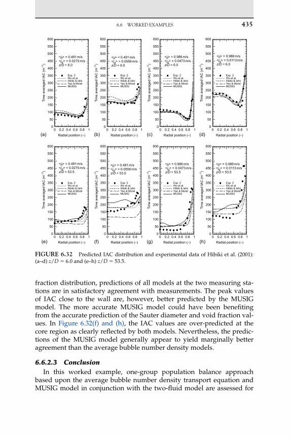
6.6 workEdExaMpLEs 435
fraction distribution, predictions of all models at the two measuring sta-tions are in satisfactory agreement with measurements. The peak values of IAC close to the wall are, however, better predicted by the MUSIG model. The more accurate MUSIG model could have been benefiting from the accurate prediction of the Sauter diameter and void fraction val-ues. In Figure 6.32(f) and (h), the IAC values are over-predicted at the core region as clearly reflected by both models. Nevertheless, the predic-tions of the MUSIG model generally appear to yield marginally better agreement than the average bubble number density models.
6.6.2.3 ConclusionIn this worked example, one-group population balance approach
based upon the average bubble number density transport equation and MUSIG model in conjunction with the two-fluid model are assessed for
Radial position (–)
Tim
e av
erag
ed IA
C (
m–1
)
0 0.2 0.4 0.6 0.8 10
50
100
150
200
250
300
350
400
450
500
550
600
Radial position (–)
Tim
e av
erag
ed IA
C (
m–1
)
0 0.2 0.4 0.6 0.8 10
50
100
150
200
250
300
350
400
450
500
550
600
Radial position (–)
Tim
e av
erag
ed IA
C (
m–1
)
0 0.2 0.4 0.6 0.8 10
50
100
150
200
250
300
350
400
450
500
550
600
Radial position (–)
Tim
e av
erag
ed IA
C (
m–1
)
0 0.2 0.4 0.6 0.8 10
50
100
150
200
250
300
350
400
450
500
550
600
Radial position (–)
Tim
e av
erag
ed IA
C (
m–1
)
0 0.2 0.4 0.6 0.8 10
50
100
150
200
250
300
350
400
450
500
550
600
Exp. 2Wu et al.Hibiki & IshiiYao & MorelMUSIG
Exp. 2Wu et al.Hibiki & IshiiYao & MorelMUSIG
Exp. 2Wu et al.Hibiki & IshiiYao & MorelMUSIG
Exp. 2Wu et al.Hibiki & IshiiYao & MorelMUSIG
Exp. 2Wu et al.Hibiki & IshiiYao & MorelMUSIG
Exp. 2Wu et al.Hibiki & IshiiYao & MorelMUSIG
Exp. 2Wu et al.Hibiki & IshiiYao & MorelMUSIG
Exp. 2Wu et al.Hibiki & IshiiYao & MorelMUSIG
(a) (b) (c) (d)
(e) Radial position (–)
Tim
e av
erag
ed IA
C (
m–1
)
0 0.2 0.4 0.6 0.8 10
50
100
150
200
250
300
350
400
450
500
550
600
(f) Radial position (–)
Tim
e av
erag
ed IA
C (
m–1
)
0 0.2 0.4 0.6 0.8 10
50
100
150
200
250
300
350
400
450
500
550
600
(g) Radial position (–)
Tim
e av
erag
ed IA
C (
m–1
)
0 0.2 0.4 0.6 0.8 10
50
100
150
200
250
300
350
400
450
500
550
600
(h)
<jf> = 0.491 m/s<jg> = 0.0275 m/sz/D = 6.0
<jf> = 0.491 m/s<jg> = 0.0275 m/sz/D = 53.5
<jf> = 0.491 m/s<jg> = 0.0556 m/sz/D = 53.5
<jf> = 0.986 m/s<jg> = 0.0473 m/sz/D = 53.5
<jf> = 0.986 m/s<jg> = 0.0113 m/sz/D = 53.5
<jf> = 0.491 m/s<jg> = 0.0556 m/sz/D = 6.0
<jf> = 0.986 m/s<jg> = 0.0473 m/sz/D = 6.0
<jf> = 0.986 m/s<jg> = 0.0113 m/sz/D = 6.0
FIgure 6.32 Predicted IAC distribution and experimental data of Hibiki et al. (2001): (a–d) z/D 6.0 and (e–h) z/D 53.5.
6. Gas–LiquidFLows436
their feasibility in handling gas–liquid bubbly flows under isothermal conditions. Three forms of the average bubble number density transport equation incorporating three coalescence and breakage mechanisms by Wu et al. (1998), Hibiki and Ishii (2002) and Yao and Morel (2004) along with the coalescence and break-up mechanisms by Prince and Blanch (1990) and Luo and Svendsen (1996) for the MUSIG model are com-pared against the experimental data of Liu and Bankoff (1993a, b) and Hibiki et al. (2001). Interfacial momentum transfer that embraces vari-ous interfacial forces including drag, lift, wall lubrication and turbulent dispersion force is also accounted for. In general, both population bal-ance approaches yield close agreement with measurements for the void fraction, IAC, mean bubble Sauter diameter and gas and liquid veloci-ties. Predictions of bubble Sauter diameter through the MUSIG model nonetheless attain remarkable agreement. This is attributed by its supe-riority in resolving the bubble size distribution as compared to the sin-gle average variable parameter through the average bubble number density models. As a result, predictions for the gas and liquid velocity of the MUSIG model are, in general, greatly enhanced and notably bet-ter. Numerical results clearly show that the dynamic changes of the bub-bles with different sizes require higher resolution and can be achieved using the MUSIG approach. As expected, the trade-off adopting such an approach is at the expense of additional computational burden in solving the extra transport equations for each bubble class. Computations using the MUSIG model are twice as slow when the average bubble number density is applied under the same computational resources. Nonetheless, predictions through average bubble number density models are found to yield satisfactory agreement with measurements, though appearing marginally inferior in some degree to the MUSIG model results. Average bubble number density models can thus be considered as a viable option especially for industrial practitioners who often demand a rapid design tool in simulating bubbly flows with reasonable accuracy. For the case of acquiring highly accurate mean bubble Sauter diameter distribution, the MUSIG model serves as the best alternative in handling such flows.
6.6.3 Sub-cooled Boiling Flow in a Vertical annulus
Sub-cooled boiling flow belongs to another special category of bubbly turbulent pipe flow which embraces the complex dynamic interactions of bubble coalescence and bubble break-up in the bulk flow as well as in the presence of heat and mass transfer occurring in the vicinity of the heated wall due to nucleation and condensation. Since the temperature in the bulk liquid remains below the saturation temperature limit, bubbles tend to decrease in size for sub-cooled boiling flow as a result of increas-ing condensation away from the heated walls. This sub-cooling effect is a

6.6 workEdExaMpLEs 437
well-known phenomenon as confirmed through Gopinath et al. (2002). Subject to this effect, sub-cooled boiling flows will certainly yield a broader range of bubble sizes and possibly even amplify dynamic changes in bubble size distribution within the flow. In addition, experimental obser-vations have confirmed that the vapour bubbles along a vertical heated wall tend to travel a short distance away from the nucleation sites, grad-ually increasing in size, before lifting off into the bulk sub-cooled liquid (Klausner et al., 1993). Such bubble motion not only alters the mode of heat transfer on the surface but also governs the departure and lift-off diame-ter of bubbles, which in turn also influences the bubble distribution in the bulk liquid. Feasible application of the population balance approach based on the MUSIG model to predict the bubble distribution in the core flow and on the improved heat wall partition model which accommodates the bubble sliding phenomenon for upwards forced convective flow is dem-onstrated through the worked examples below. Experimental data of iso-thermal gas–liquid bubbly flow in a vertical pipe performed by Yun et al. (1997) and Lee et al. (2002) are utilized to validate the numerical model.
For the sub-cooled boiling experiments by Yun et al. (1997) and Lee et al. (2002), the experimental set-up consists of a vertical concentric annulus with an inner rod of 19 mm outer diameter uniformly heated by a 54 kW DC power supply. This heated section comprises of a 1.67 m long Inconel 625 tube with a 1.5 mm wall thickness filled with magne-sium oxide powder insulation. The outer wall comprised of two stainless steel tubes with 37.5 mm inner diameter. De-mineralized water is used as the working fluid. Local gas phase parameters such as radial distribution of the void fraction, bubble frequency and bubble velocity are measured by a two-conductivity probe method located 1.61 m downstream of the beginning of the heated section. The bubble Sauter diameters (assuming spherical bubbles) are determined through the IAC which is calculated using the measured bubble velocity spectrum and bubble frequency. Figure 6.33 shows the schematic drawing of the test channel.
6.6.3.1 Application of MUSIG Boiling ModelThis worked example demonstrates the population balance approach
based upon the application of a MUSIG boiling model which incorporates the important phenomenology of nucleation and condensation processes for sub-cooled boiling flows at low pressures. In addition, considerations for the coalescence and break-up mechanisms are modelled by the work conducted by Prince and Blanch (1990) and Luo and Svendsen (1996) to predict the bubble size distribution within the bulk liquid.
Numerical FeaturesIn modelling sub-cooled gas–liquid bubbly flow, numerical solu-
tions are obtained from two sets of transport equations governing the

6. Gas–LiquidFLows438
conservation of mass, momentum and energy, with all six equations accompanied by relevant interfacial terms. Firstly, mass and heat-transfer rates due to condensation in the bulk sub-cooled liquid are considered. Secondly, momentum transfer involving drag force, lift force, wall lubri-cation force and turbulent dispersion force are considered. The drag force is calculated according to equations (6.14) and (6.15) in which the drag coefficient CD is calculated based on the correlation by Ishii and Zuber (1979) for several distinct Reynolds number regions. The lift force is described in terms of the slip velocity and the curl of the liquid phase velocity according to equation (6.25) where a constant CL of 0.01 is prescribed (Wang et al., 1987). The wall lubrication force takes the form that has been derived by Antal et al. (1991) – equation (6.28) – where the
Measurementplane
1610 mmhigh
1670 mmlong
heatedsection
Heated innertubeOD 19 mm
Isothermalouter wallID 37.5 mm
Inlet liquidflow
FIgure 6.33 Schematic drawing of a heated vertical upward annular flow.

6.6 workEdExaMpLEs 439
constants Cw1 and Cw2 take on values of 0.01 and 0.05, respectively. The turbulent dispersion force takes the form according to Antal et al. (1991) – equation (6.30) – where the recommended value for CTD according to Kurul and Podowski (1990) of 0.1 is used.
The discretized equations are solved using Stone’s (1968) Strongly Implicit Procedure (SIP) with advection and diffusion terms approxi-mated by the hybrid differencing and CD schemes. Velocity–pressure linkage is handled through the Inter-Phase Slip Algorithm (IPSA) which is a variant of the Semi-Implicit for Method Pressure-Linkage Equations (SIMPLE) procedure for the computation of the bubbly flows in the context of computational fluid dynamics. To account for the turbulence within the flow channel, a two-equation standard k–e model is employed for the continuous liquid phase. The effective viscosity in the momentum and energy equations is taken as the sum of the molecular viscosity and turbulent viscosity of which the turbulent viscosity is considered as the total of the shear-induced turbulent viscosity and Sato’s bubble-induced turbulent viscosity (Sato et al., 1981). Since logarithmic wall function is employed to bridge the wall and the fully turbulent region away from the heater surface, the normal distance between the wall and the first node in the bulk sub-cooled liquid should be such that the correspond-ing dimensionless distance x is greater than 30.
To account for the non-uniform bubble size distribution in the bulk sub-cooled liquid, bubbles ranging from 0 to 9.5 mm diameter are equally divided into 15 size groups (see Table 6.6). These discrete bubble sizes are subsequently tracked by solving an additional set of 15 transport equa-tions which are progressively coupled with the flow equations during the simulations. Sensitivity study on the number of size groups is performed through the consideration of equally dividing the bubble diameters into 10, 15 and 20 size groups. The analysis reveals that no appreciable dif-ference is found for the predicted maximum bubble Sauter diameter between the 15 and 20 bubble size groups. For the sub-division into 10 size groups, the maximum bubble Sauter diameter is under-predicted by a maximum difference of 2%. In view of the computational resources and times, it is therefore concluded that the sub-division of the bubbles sizes into 15 size groups is deemed sufficient and hereafter in the following the computational results are all based on the discretization of 15 bubble size groups.
A body-fitted conformal system is employed to generate the three-dimensional mesh within the annular channel resulting in a total of 13 (radial) 30 (axial) 3 (circumference) control volumes. Grid inde-pendence is examined. In the mean parameters considered, further grid refinement does not reveal any significant changes to the two-phase flow parameters. Convergence is achieved within 1500 iterations when the mass residual drops below 1.0 107.

6. Gas–LiquidFLows440
Numerical ResultsIn this worked example, the mechanistic model of Kurul and
Podowski (1990), which consists of partitioning the wall heat flux into three heat flux components, namely surface quenching, vapour genera-tion and turbulent convection, is adopted. To achieve closure, the bub-ble departure diameter, density of active nucleation sites and bubble departure frequency are required to be specified. For the current model, the bubble departure diameter, density of active nucleation sites and bubble departure frequency are evaluated according to the proposals by Kocamustafaogullari and Ishii (1995) correlation with a bubble contact of 55° as suggested in Hsu and Graham (1976) for most industrial metals and water, Lemmert and Chwala’s (1977) and Cole (1960), respectively.
In addition, comparison of the MUSIG boiling model is also compared against computational results determined through the empirical relation-ship of Anglart and Nylund (1996) to determine the local bubble diam-eter. This relationship is still being used in the CFX4.4 code. In this present investigation, the existing model will be known as the default boiling model. The empirical bubble departure correlation in the wall heat partition
taBle 6.6 diametersofEachdiscretebubbleClassforMusiGModel
Class no.Central class diameter
(mm)
1 0.503
2 1.040
3 1.644
4 2.265
5 2.889
6 3.512
7 4.141
8 4.771
9 5.402
10 6.033
11 6.665
12 7.297
13 7.929
14 8.562
15 9.194

6.6 workEdExaMpLEs 441
model employs the relationship of Tolubinsky and Kostanchuk (1970) (built-in into the default boiling model). Reference diameters of d1 and d2 for the empirical relationship of Anglart and Nylund (1996) such as those described in equation (6.145) corresponding to the reference sub-cooling temperatures at Tsub,1 and Tsub,2 are usually not known a priori. The local bubble diameters are assumed to be evaluated between d1 1.5 104 m and d2 7.0 103 m with further assumption of both reference diame-ters corresponding to reference sub-cooling temperatures of Tsub,1 13.0 K and Tsub,2 5 K. In Tu and Yeoh (2002), improvements are made to the sub-cooled boiling flow model to better predict the axial void fraction dis-tribution. The mean bubble diameter relationship of Zeitoun and Shoukri (1996a) such as expressed in equation (6.146) is incorporated (here referred to as the modified boiling model).
Experimental conditions that are used for comparison with the simu-lated results are presented in Table 6.7. The radial profiles of the bubble Sauter diameter, void fraction, interfacial area and vapour and liquid velocities located at 1.61 m downstream of the beginning of the heated section are predicted. In all the figures presented, the dimension-less parameter (r Ri)/(Ro Ri) 1 indicates the inner surface of the unheated flow channel wall, while (r Ri)/(Ro Ri) 0 indicates the surface of the heating rod in the annulus channel.
Figure 6.34 illustrates the local radial bubble Sauter diameter distribu-tion at the measuring plane of the heated annular channel. In all the three cases, the empirical correlations from the default and modified boiling models grossly misrepresent the local bubble sizes. The gradual increase of the bubble Sauter diameters towards the heated wall with the highest bubble sizes at the heated wall by the empirical relationships contradicts the local radial measurements. According to the experimental observa-tion in Figures 6.13 and 6.14, large bubble sizes present away from the heated wall are correctly predicted by the MUSIG boiling model for all the three experimental conditions. It is clearly evident that the empiri-cal correlation is deficient in predicting the local bubble distribution due to the absence of properly accommodating the bubble mechanistic
taBle 6.7 ExperimentalConditions
Run Pinlet (MPa) Tinlet (°C) Tsub (°C) Qw (kW/m2) G (kg/(m2 s))
C1 0.142 96.6 13.4 152.3 474.0
C2 0.137 94.9 13.8 197.2 714.4
C3 0.143 92.1 17.9 251.5 1059.2
Note: Pinlet: inlet pressure, Tinlet: inlet temperature, Tsub: inlet sub-cooling temperature, Qw: wall heat flux and G: inlet mass flux.

6. Gas–LiquidFLows442
0
1
2
3
4
5
6
(r–Ri)/(Ro–Ri)
Sa
ute
r d
iam
ete
r (m
m)
Measurement
MUSIG boiling modelModified boiling model
Default boiling model
0 0.2 0.4 0.6 0.8 1
Qwall = 197.2 kW/m2
Tinlet = 95.0°CPinlet = 0.137 MPaG = 714.4 kg/m2s
Measurement
MUSIG boiling modelModified boiling model
Default boiling model
0
1
2
3
4
5
6
(r–Ri)/(Ro–Ri)(a)
(b)
(c)
Sa
ute
r d
iam
ete
r (m
m)
0 0.2 0.4 0.6 0.8 1
Qwall = 152.9 kW/m2
Tinlet = 96.6°CPinlet = 0.142 MPaG = 474.0 kg/m2s
0
1
2
3
4
5
6
(r–Ri)/(Ro–Ri)
Sa
ute
r d
iam
ete
r (m
m)
0 0.2 0.4 0.6 0.8 1
Measurement
MUSIG boiling modelModified boiling model
Default boiling model
Qwall = 197.2 kW/m2
Tinlet = 95.0°CPinlet = 0.137 MPaG = 714.4 kg/m2s
FIgure 6.34 Local mean radial profiles of bubble Sauter diameter for cases C1, C2 and C3.

6.6 workEdExaMpLEs 443
behaviour coalescence and collapse due to condensation. Evidently, the bubble size determination in the bulk liquid core is strictly dependent on the local sub-cooling temperatures alone. In all the three cases, a maxi-mum predicted bubble size is, respectively, obtained for C1, C2 and C3 of about 4.5, 4.0 and 3.8 mm through the MUSIG boiling model confirming the experimental observations. As the bubbles migrate towards the oppo-site end of the adiabatic wall, they decrease due to the increased action of condensation. Here, only single-phase sub-cooled water exists. The bub-ble Sauter diameter profiles of the MUSIG boiling model clearly show the gradual collapse of the bubbles and the absence of bubbles near the adia-batic wall of the test channel. Another important observation to the effect of condensation shows that more bubbles are condensed with a higher inlet sub-cooling condition, as shown in Figure 6.34(c). With increasing mass fluxes, interfacial heat transfer is further enhanced, thereby result-ing in more bubbles being condensed in the sub-cooled liquid core.
Locally predicted void fraction profiles against radial measured val-ues are depicted in Figure 6.35. Peak local void fraction always exits in the vicinity of the heated surface in a typical sub-cooled boiling flow due to the large number of bubbles generated from the active nucleation sites on the heated surface. Here, a large amount of bubbles is generated from these nucleation sites when the temperature on the heated surface exceeds the saturation temperature. As these bubbles reach a critical size, they detach and migrate laterally towards the sub-cooled liquid core under the competing processes of bubble coalescence and condensation. The default and modified boiling models under-predict the void fraction profiles for all three experimental conditions, the most severe being case C3 where the channel boiling flow is subjected to high inlet sub-cooling and mass flux conditions (see Figure 6.35(c)). Figure 6.36 describes the local IAC radial distribution. The measured radial data follow a simi-lar trend as the void fraction distribution in Figure 6.35. Overall, better agreement between the measured and predicted IAC is achieved using the MUSIG boiling model. Here again, the default and modified boiling models under-predict the IAC by an unacceptable margin.
The radial profiles of the local vapour velocity and liquid velocity are shown in Figures 6.37 and 6.38, respectively, for experimental condi-tions C1, C2 and C3. The vapour velocity is greater than the liquid veloc-ity due to action of the buoyancy force caused by density difference. As observed in the experiment, the vapour velocity was higher at the cen-tre than the velocities near the heating rod. This was probably due to the buoyancy effect being enhanced for the migration of the large bubbles there. However, the vapour velocity predicted by the MUSIG boiling model along with the default and modified models shows higher veloci-ties approaching the heated boundary. The MUSIG boiling model vapour velocities in the vicinity of the heated surface are rather similar to those

6. Gas–LiquidFLows444
Measurement
MUSIG boiling modelModified boiling model
Default boiling model
Qwall = 152.9 kW/m2
Tinlet = 96.6°CPinlet = 0.142 MPaG = 474.0 kg/m2s
Qwall = 197.2 kW/m2
Tinlet = 95.0°CPinlet = 0.137 MPaG = 714.4 kg/m2s
(r–Ro)/(Ri–Ro)(a)
(b)
(c)
(r–Ro)/(Ri–Ro)
0 0.2 0.4 0.6 0.8 10
0.1
0.2
0.3
0.4
0.5
Voi
d fr
actio
n
Measurement
MUSIG boiling modelModified boiling model
Default boiling model
0 0.2 0.4 0.6 0.8 10
0.1
0.2
0.3
0.4
0.5
Voi
d fr
actio
n
Qwall = 251.5 kW/m2
Tinlet = 92.1°CPinlet = 0.143 MPaG = 1059.2 kg/m2s
(r–Ro)/(Ri–Ro)
Measurement
MUSIG boiling modelModified boiling model
Default boiling model
0 0.2 0.4 0.6 0.8 10
0.1
0.2
0.3
0.4
0.5
Voi
d fr
actio
n
FIgure 6.35 Local mean radial profiles of void fraction for cases C1, C2 and C3.

6.6 workEdExaMpLEs 445
0
200
400
600
800
IAC
(1/
m)
0 0.2 0.4 0.6 0.8 1
0
200
400
600
800
IAC
(1/
m)
0 0.2 0.4 0.6 0.8 1
0
200
400
600
800
IAC
(1/
m)
0 0.2 0.4 0.6 0.8 1
MeasurementMUSIG boiling modelModified boiling modelDefault boiling model
MeasurementMUSIG boiling modelModified boiling modelDefault boiling model
MeasurementMUSIG boiling modelModified boiling modelDefault boiling model
(r–Ri)/(Ro–Ri)
(r–Ri)/(Ro–Ri)
(r–Ri)/(Ro–Ri)
Qwall = 251.5 kW/m2
Tinlet = 92.1°CPinlet = 0.143 MPaG = 1059.2 kg/m2s
Qwall = 152.9 kW/m2
Tinlet = 96.6°CPinlet = 0.142 MPaG = 474.0 kg/m2s
Qwall = 197.2 kW/m2
Tinlet = 95.0°CPinlet = 0.137 MPaG = 714.4 kg/m2s
FIgure 6.36 Local mean radial profiles of IAC for cases C1, C2 and C3.

6. Gas–LiquidFLows446
0
0.2
0.4
0.6
0.8
1
1.2
1.4
Vap
our
velo
city
(m
/s)
0 0.2 0.4 0.6 0.8 1(r–Ri)/(Ro–Ri)
MeasurementMUSIG boiling modelModified boiling modelDefault boiling model
0.2
0.4
0.6
0.8
1
1.2
1.4
1.6
1.8
Vap
our
velo
city
(m
/s)
0 0.2 0.4 0.6 0.8 1(r–Ri)/(Ro–Ri)
MeasurementMUSIG boiling modelModified boiling modelDefault boiling model
0.4
0.6
0.8
1
1.2
1.4
1.6
1.8
2
Vap
our
velo
city
(m
/s)
0 0.2 0.4 0.6 0.8 1(r–Ri)/(Ro–Ri)
MeasurementMUSIG boiling modelModified boiling modelDefault boiling model
Qwall = 251.5 kW/m2
Tinlet = 92.1°CPinlet = 0.143 MPaG = 1059.2 kg/m2s
Qwall = 152.9 kW/m2
Tinlet = 96.6°CPinlet = 0.142 MPaG = 474.0 kg/m2s
Qwall = 197.2 kW/m2
Tinlet = 95.0°CPinlet = 0.137 MPaG = 714.4 kg/m2s
FIgure 6.37 Local mean radial profiles of vapour velocity for cases C1, C2 and C3.

6.6 workEdExaMpLEs 447
0
0.2
0.4
0.6
0.8
1
1.2
1.4
Liqu
id v
eloc
ity (
m/s
)
0 0.2 0.4 0.6 0.8 1(r–Ri)/(Ro–Ri)
MeasurementMUSIG boiling modelModified boiling modelDefault boiling model
0 0.2 0.4 0.6 0.8 1
(r–Ri)/(Ro–Ri)
0.4
0.6
0.8
1
1.2
1.4
1.6
1.8
2
Liqu
id v
eloc
ity (
m/s
)
MeasurementMUSIG boiling modelModified boiling modelDefault boiling model
Qwall = 251.5 kW/m2
Tinlet = 92.1°CPinlet = 0.143 MPaG = 1059.2 kg/m2s
Qwall = 152.9 kW/m2
Tinlet = 96.6°CPinlet = 0.142 MPaG = 474.0 kg/m2s
0.2
0.4
0.6
0.8
1
1.2
1.4
1.6
1.8
Liqu
id v
eloc
ity (
m/s
)
0 0.2 0.4 0.6 0.8 1(r–Ri)/(Ro–Ri)
MeasurementMUSIG boiling modelModified boiling modelDefault boiling model
Qwall = 197.2 kW/m2
Tinlet = 95.0°CPinlet = 0.137 MPaG = 714.4 kg/m2s
FIgure 6.38 Local mean radial profiles of liquid velocity for cases C1, C2 and C3.

6. Gas–LiquidFLows448
of the simpler models for all three cases because of the assumption that each bubble class travels at the same mean algebraic velocity. Within the channel space, different size bubbles are expected to travel with differ-ent speeds. Additional momentum equations or an algebraic slip model could be employed to resolve the problem. It should be noted that the consideration of additional momentum equations to cater for each of the 15 bubble classes would increase the computational resources tremen-dously and deem impractical. The inhomogeneous MUSIG model, which caters for the possibility of solving momentum equations for a pertinent choice of two or three dominant groups of bubbles to sufficiently accom-modate the hydrodynamics of a wide bubble size distribution of bubbly flows, may be adopted. For the algebraic slip model, the terminal veloci-ties for each of the bubbles may be determined through an algebraic rela-tionship suggested by Clift et al. (1978). Nevertheless, in Figure 6.38, the MUSIG boiling model predictions of the liquid velocities are better repre-sented when compared against the experimental measurements.
ConclusionIn this worked example, a two-fluid model coupled with the popula-
tion balance approach is presented in handling sub-cooled boiling flows at low pressures. The increase in complexity in modelling such flows is borne from the additional consideration of phase change due to condensa-tion. The range of bubble sizes in the sub-cooled boiling flow is distributed according to the division of 15 diameter groups through the formulation of a MUSIG boiling model with the consideration of bubble coalescence by Prince and Blanch (1990) and bubble break-up by Luo and Svendsen (1997). Comparison of the predicted results is made against recent local measurements of Yun et al. (1997) and Lee et al. (2002). Additional com-parison is also performed against the existing boiling model in CFX4.4 and the modified boiling model developed in Tu and Yeoh (2002). Good agree-ment is achieved through the MUSIG boiling model for the local bubble Sauter diameter, void fraction, IAC and liquid velocity profiles. However, in the gas phase, since the assumption is invoked where each bubble class travels at the same mean algebraic velocity in order to reduce the compu-tational time and resources, significant weakness of the model is evident in the prediction of the vapour velocity. Possible application of the inhomo-geneous MUSIG model or an algebraic slip model to account for bubble separation could yield a more realistic prediction of the vapour velocity.
6.6.3.2 Application of Improved Wall Heat Partition ModelThis worked example focuses on the increasing physics that is considered
for the nucleation process at the heated wall through the improved wall heat partition model. Away from the heated wall, the model is coupled with the MUSIG boiling model in order to aptly predict the bubble size distribution.

6.6 workEdExaMpLEs 449
Numerical FeaturesThe two-fluid model which is based on solving two sets of equations
governing the conservation of mass, momentum and energy is solved. For the interfacial terms, mass and heat transfer for the condensation in the bulk sub-cooled liquid and momentum transfer due to drag force and non-drag forces such as lift, wall lubrication and turbulent dispersion are considered. The coefficients and constants for the drag and non-drag forces are identical to those applied in the previous worked example.
In this worked example, the improved wall heat partition model described in Section 6.5.3 is applied instead of the mechanistic model of Kurul and Podowski (1990). The improved model consists of additional partitioning of the wall heat flux to accommodate for the bubble sliding phenomenon, the force balance model in determining departing bubble diameters – size of bubbles lifting off the heated wall and departing from the cervices of the heated wall and a mechanistic model to ascertain the bubble frequency based on the ebullition cycle theory in nucleate boiling. The bubble contact angle is taken to be at 35°.
Stone’s (1968) SIP is employed with the application of hybrid differenc-ing and CD schemes to approximate the advection and diffusion terms. Velocity–pressure coupling is achieved through the IPSA. A two-equation standard k–e turbulent model is employed for the continuous liquid phase. The effective viscosity in the momentum and energy equations is taken as the sum of the molecular viscosity and turbulent viscosity of which the turbulent viscosity is considered as the total of the shear-induced turbu-lent viscosity and Sato’s bubble-induced turbulent viscosity (Sato et al., 1981). Logarithmic wall function is employed to bridge the wall and the fully turbulent region away from the heater surface with the normal dis-tance between the wall and the first node in the bulk sub-cooled liquid corresponding to a dimensionless distance x greater than 30.
Similar to the previous worked example, a total number of 15 bubble classes are prescribed for the dispersed phase (see Table 6.6). This repre-sents an additional set of 15 transport equations which is progressively solved and coupled with the flow equations during the simulations. A body-fitted conformal mesh resulting in a total of 13 (radial) 30 (axial) 3 (circumference) control volumes is generated. Grid indepen-dence is examined and in the mean parameters considered, further grid refinement did not reveal any significant changes to the two-phase flow parameters. Convergence is achieved within 1500 iterations when the mass residual drops below 1.0 107.
Numerical ResultsExperimental conditions that are used for comparison with the simu-
lated results are the same conditions presented in Table 6.7 with the same measuring location for the comparison of the radial profiles of the bubble Sauter diameter, void fraction and IAC.

6. Gas–LiquidFLows450
Figure 6.39 illustrates the predicted Sauter mean bubble diameter pro-files at the measuring plane of the heated annular channel. For all three cases, the bubble size changes are found to be adequately predicted. Observed consistent trends between the predicted and measured Sauter mean bubble diameter reflect the measure of the MUSIG boiling model in aptly capturing the bubble coalescence especially in the vicinity of the heated wall. The development of bubbles in this region stems from the evaporation process occurring at the heated wall and forces acting on the vapour bubbles determining the bubble size at departure or lift off.
Table 6.8 illustrates the various contributing heat flux components and the associated bubble departure and lift-off diameters evaluated by the improved heat partition model. On the basis of the force balance model, the bubble departure diameters are predicted with a size of approxi-mately 0.56–0.58 mm, while the lift-off diameters are found within a range of 1.2–1.45 mm. The ratio between the bubble lift-off diameter (Dl)
Sau
ter
mea
n bu
bble
dia
met
er (
m)
(r–Ri)/(Ro–Ri)
0 0.2 0.4 0.6 0.8 1
MeasurementMUSIG boiling
0
0.002
0.004
0.006
0.008
Case C3
(r–Ri)/(Ro–Ri)
Sau
ter
mea
n bu
bble
dia
met
er (
m)
0 0.2 0.4 0.6 0.8 10
0.002
0.004
0.006
0.008
MeasurementMUSIG boiling
Case C1
Sau
ter
mea
n bu
bble
dia
met
er (
m)
(r–Ri)/(Ro–Ri)
0 0.2 0.4 0.6 0.8 1
MeasurementMUSIG boiling
0
0.002
0.004
0.006
0.008
Case C2
FIgure 6.39 Prediction of mean Sauter diameter distribution and experimental data at the measuring station.

6.6 workEdExaMpLEs 451
and bubble departure diameter (Dd) is thus determined to be between 2 and 3 mm, which is closely corresponded to experimental observations of Basu et al. (2002). Surface quenching due to sliding bubbles and evapora-tion are found to be the dominant modes of heat transfer governing the heat partition model. The former highlighted the prevalence of bubble sliding motions on the surface significantly altering the rate of heat trans-fer and subsequently the resultant vapour generation rate. Away from the heated wall, bubbles entering the bulk sub-cooled liquid were con-densed due to the sub-cooling effect. Predicted trends of the Sauter mean diameter profiles clearly show the gradual collapse of the bubbles from the channel centre to the outer unheated wall.
Although the measured bubble sizes near the heated wall are found to agree quite well with the measured data, confirming to a certain extent the appropriate estimation of the bubble lift-off diameters, a closer examination of the local void fraction profiles at the measuring station in Figure 6.40 indicates a less than satisfactory prediction of the void fraction near the heated surface where they are either over-predicted or under-predicted, as denoted in cases C1 and C3. The void fraction distri-bution in case C2 nonetheless compares reasonably well with measure-ment. This discrepancy could be attributed to the uncertainties within the heat partition model in being able to specifically evaluate the vapour generation rate. In the quest for reducing the application of empirical correlations, the consideration of the active nucleation site density in the present study is still dependent on the use of an appropriate relationship, which could be sensitive to flow conditions. The population of cavities on the heated wall may vary significantly between materials and cannot be measured directly. Therefore, what cannot be measured cannot be pre-scribed. An adequate expression of the active nucleation site density cov-ering a wide range of flow conditions remains outstanding and requires further investigation. The IAC as shown in Figure 6.41 also exhibits simi-lar trends with the void fraction distributions.
taBle 6.8 predictedHeatpartitions,bubbledepartureandLift-offdiameterofsub-CooledboilingFlowConditions
Measuring location C1 C2 C3
Qc (W/m2) 0% 0% 0%
Qtc (W/m2) 2.51% 4.56% 6.42%
Qtcsl (W/m2) 55.07% 61.25% 65.58%
Qe (W/m2) 42.42% 34.19% 28.00%
Dd (mm) 0.56 0.58 0.57
Dl (mm) 1.45 1.31 1.20

6. Gas–LiquidFLows452
Figure 6.42 shows the bubble size distribution expressed in terms of IAC of individual bubbles classes along the radial direction for the case C3. Significant vapour bubbles that are represented from bubble class 3 in the vicinity of the heated wall essentially indicate the size of the bubble lift-off diameter which coalesce with downstream/neighbour-ing bubbles forming larger void fraction peaks as indicated by bubble classes 7 and 9. Owing to the high shear stress within the boundary layer, some bubbles are affected by turbulent impact due to breakage resulting in the formation of smaller bubbles as evident by the significant distri-butions indicated within bubble classes 1 and 2. Away from the heated wall, the condensation process dominates in reducing the void fraction of each bubble class, eventually collapsing the majority of the bubbles beyond the position (r Ri)/(Ro Ri) 0.6. The net generation rate due to coalescence and breakage and condensation rate of selected bubble
Case C3
0
0.1
0.2
0.3
0.4
0.5
Tim
e av
erag
ed g
as v
oid
frac
tion
(–)
(r–Ri)/(Ro–Ri)
0 0.2 0.4 0.6 0.8 1
MeasurementMUSIG boiling
Case C1
Tim
e av
erag
ed g
as v
oid
frac
tion
(–)
0
0.1
0.2
0.3
0.4
0.5
(r–Ri)/(Ro–Ri)
0 0.2 0.4 0.6 0.8 1
MeasurementMUSIG boiling
MeasurementMUSIG boiling
Tim
e av
erag
ed g
as v
oid
frac
tion
(–)
0
0.1
0.2
0.3
0.4
0.5
(r–Ri)/(Ro–Ri)
0 0.2 0.4 0.6 0.8 1
Case C2
FIgure 6.40 Predicted radial void fraction distribution and experimental data at the measuring station.

6.6 workEdExaMpLEs 453
classes are depicted in Figure 6.43. Close to the wall region, the highest generation rate corresponding to the peak value observed in Figure 6.42 is represented by bubble class 7; substantial generation rate is also found for bubble class 3 at the same region. While the coalescence of bubbles is seen to be governed mainly by bubble classes 3 and 7, bubble classes 3 and 12 also contribute to the condensation process due to their consider-ably high number density and interfacial area. These two figures aptly demonstrate the mechanisms of coalescence, breakage and condensation in the MUSIG boiling model affecting the thermo-mechanical and hydro-dynamics processes within the sub-cooled boiling flow at low pressures.
ConclusionIn this worked example, the improved wall heat flux partitioning model
that accounts for sliding bubbles alongside the fundamental consideration
Case C1
IAC
(1/
m)
0
200
400
600
800
MeasurementMUSIG boiling
(r–Ri)/(Ro–Ri)
0 0.2 0.4 0.6 0.8 1
Case C2
IAC
(1/
m)
0
200
400
600
800
MeasurementMUSIG boiling
(r–Ri)/(Ro–Ri)
0 0.2 0.4 0.6 0.8 1
Case C3
IAC
(1/
m)
0
200
400
600
800
MeasurementMUSIG boiling
(r–Ri)/(Ro–Ri)
0 0.2 0.4 0.6 0.8 1
FIgure 6.41 Prediction of IAC distribution and experimental data at the measuring station.

6. Gas–LiquidFLows454
1 2 3 4 5 6 7 8 9 10 11 12 1314
15 0.8
0.6
0.4
0.20.05
1
2
34 5
6
7
8 9
10
11 12 13 14 15
12
35
6
7
9
1011 12 13 14 15
12 3 4 5 6 7
8 910 11 12 13 14 15
12 3 4 5 6 7 8 9 10 11 12 13 14 15
1 2 3 4 5 6 7 8 9 10 11 12 13 14 15
0.00E+00
1.00E+01
2.00E+01
3.00E+01
4.00E+01
5.00E+01
6.00E+01
7.00E+01
8.00E+01
9.00E+01
1.00E+02
IAC
(–)
Bubble class
Radial location
Case C3
4
8
FIgure 6.42 Predicted IAC of each bubble class along the radial direction for the case C3 at the measuring station.
(r–Ri)/(Ro–Ri)
Net
gen
erat
ion
rate
(kg
/m3 s
)
0 0.2 0.4 0.6 0.8 1–1.5
–1
–0.5
0
0.5
1
1.5
2
2.5
3
Net rate Class 3Net rate Class 7Net rate Class 12Condensation Class 3Condensation Class 7Condensation Class 12
Case C3
FIgure 6.43 Predicted net bubble generation rate due to coalescence and breakage and condensation rate of selected bubble classes of the MUSIG boiling model.
6.7 suMMary 455
of bubble frequency theory coupled with a force balance model to predict forces acting on a vapour bubble growing under the sub-cooled boiling flow condition demonstrates the capability of accommodating more com-plex analyses of bubble growth, bubble departure, bubble lift-off over a wide range of wall heat fluxes and flow conditions. In conjunction with the MUSIG boiling model, remarkable agreement is achieved for the local profiles of the void fraction, Sauter mean diameter and IAC for different experimental conditions.
6.7 SuMMary
Gas–liquid flows are considered in this chapter. Within this flow sys-tem, the two phases that co-exist simultaneously in the fluid flow often exhibit relative motion among the phases and heat and mass exchanges across the interface boundary. Owing to the complexities of interfaces and resultant discontinuities in fluid properties as well as from physical scal-ing issues, it is rather customary to apply a statistical, averaged approach in the form of a two-fluid model to resolve such a flow system. Separate transport equations governing the conservation of mass, momentum and energy are solved for each phase and exchanges that take place at the interfaces between the two phases are explicitly accounted for in which the dynamics of the interaction between the two phases can be effec-tively described via suitable models of the inter-phase mass, momentum and energy exchanges. Normally, the coupling between the two phases is very tight, which demands special numerical strategies and solution algorithms to be adopted. This particular flow system is also compli-cated considerably by the prevalence of particle–particle collisions. A number of population balance methods along with suitable coalescence and break-up mechanisms are discussed. In the context of computational fluid dynamics, the application of population balance models to describe the coalescence and break-up dynamics of these gas particles can be cou-pled with the two-fluid model to predict the wide range of particle sizes within the two-phase flow.
The analyses of gas–liquid flows with and without heat and mass transfer are exemplified through the worked examples of isothermal and sub-cooled boiling bubbly flows. For dispersed isothermal bubbly flows (gas–liquid flows without heat and mass transfer) in a rectangular col-umn, the non-drag forces – lift, wall lubrication and turbulent dispersion forces – have been found to exert a stabilizing effect to the two-phase flow structure. For isothermal bubbly flows (gas–liquid flows without heat and mass transfer) in a vertical pipe, predictions of the local bubble size distributions are adequately attained through the population bal-ance models for a range of flow conditions. For sub-cooled boiling flows
6. Gas–LiquidFLows456
(gas–liquid flows with heat and mass transfer) in an annulus with the inner wall being heated, the application of the two-fluid model, popula-tion balance model with further consideration of the condensation effect in addition to the bubble coalescence and break-up mechanistic behav-iours, and the wall heat partition model to characterize the nucleation of bubbles at the heated wall clearly demonstrates the feasibility of adopt-ing the statistical, averaged approach to resolve such flows.