computational study of peptide permeation through membrane: searching for hidden slow variables
TRANSCRIPT

This article was downloaded by: [New York University]On: 17 September 2013, At: 03:29Publisher: Taylor & FrancisInforma Ltd Registered in England and Wales Registered Number: 1072954 Registered office: Mortimer House,37-41 Mortimer Street, London W1T 3JH, UK
Molecular Physics: An International Journal at theInterface Between Chemistry and PhysicsPublication details, including instructions for authors and subscription information:http://www.tandfonline.com/loi/tmph20
Computational study of peptide permeation throughmembrane: Searching for hidden slow variablesAlfredo E. Cardenas a & Ron Elber a ba Institute for Computational Engineering and Sciences , University of Texas at Austin ,Austin , TX , 78712 , USAb Department of Chemistry and Biochemistry , University of Texas at Austin , Austin , TX ,78712 , USAAccepted author version posted online: 09 Sep 2013.
To cite this article: Molecular Physics (2013): Computational study of peptide permeation through membrane: Searchingfor hidden slow variables, Molecular Physics: An International Journal at the Interface Between Chemistry and Physics, DOI:10.1080/00268976.2013.842010
To link to this article: http://dx.doi.org/10.1080/00268976.2013.842010
Disclaimer: This is a version of an unedited manuscript that has been accepted for publication. As a serviceto authors and researchers we are providing this version of the accepted manuscript (AM). Copyediting,typesetting, and review of the resulting proof will be undertaken on this manuscript before final publication ofthe Version of Record (VoR). During production and pre-press, errors may be discovered which could affect thecontent, and all legal disclaimers that apply to the journal relate to this version also.
PLEASE SCROLL DOWN FOR ARTICLE
Taylor & Francis makes every effort to ensure the accuracy of all the information (the “Content”) containedin the publications on our platform. However, Taylor & Francis, our agents, and our licensors make norepresentations or warranties whatsoever as to the accuracy, completeness, or suitability for any purpose of theContent. Any opinions and views expressed in this publication are the opinions and views of the authors, andare not the views of or endorsed by Taylor & Francis. The accuracy of the Content should not be relied upon andshould be independently verified with primary sources of information. Taylor and Francis shall not be liable forany losses, actions, claims, proceedings, demands, costs, expenses, damages, and other liabilities whatsoeveror howsoever caused arising directly or indirectly in connection with, in relation to or arising out of the use ofthe Content.
This article may be used for research, teaching, and private study purposes. Any substantial or systematicreproduction, redistribution, reselling, loan, sub-licensing, systematic supply, or distribution in anyform to anyone is expressly forbidden. Terms & Conditions of access and use can be found at http://www.tandfonline.com/page/terms-and-conditions

1
Computational study of peptide permeation through membrane:
Searching for hidden slow variables
Alfredo E. Cardenasa* and Ron Elbera,b*
aInstitute for Computational Engineering and Sciences, bDepartment of Chemistry and
Biochemistry, University of Texas at Austin, Austin TX 78712, USA
*Corresponding authors. Emails: [email protected]; [email protected]
Accep
ted M
anus
cript
Dow
nloa
ded
by [
New
Yor
k U
nive
rsity
] at
03:
29 1
7 Se
ptem
ber
2013

2
Computational study of peptide permeation through membrane:
Searching for hidden slow variables
Atomically detailed molecular dynamics trajectories in conjunction with
Milestoning are used to analyze the different contributions of coarse variables to
the permeation process of a small peptide (N-acetyl-L-tryptophanamide, NATA)
through a 1,2-dioleoyl-sn-glycero-3-phosphocholine (DOPC) membrane. The
peptide reverses its overall orientation as it permeates through the biological
bilayer. The large change in orientation is investigated explicitly but is shown to
impact the free energy landscape and permeation time only moderately.
Nevertheless, a significant difference in permeation properties of the two halves
of the membrane suggests the presence of other hidden slow variables. We
speculate, based on calculation of the potential of mean force, that a
conformational transition of NATA makes significant contribution to these
differences. Other candidates for hidden slow variables may include water
permeation and collective motions of phospholipids.
Keywords: Passive permeation; Membrane simulations; Milestoning; hidden
slow variables; mean first passage time
1. Introduction
Permeation of small molecules through membranes has attracted considerable
experimental and theoretical attention in the past [1-9]. Determination of permeation
coefficients and rates of small molecules through biological membranes is clearly
important for evolutionary studies [4,6], for investigations of pollutants [10-13], and for
research of drug delivery [14-17]. In the present manuscript we focus on the passive
permeation of a small peptide through a membrane. Amino acids are the building blocks
Accep
ted M
anus
cript
Dow
nloa
ded
by [
New
Yor
k U
nive
rsity
] at
03:
29 1
7 Se
ptem
ber
2013

3
of proteins and their transport into primitive cells that lacks transport machinery is
necessary fuel for protein synthesis. Experimentally we note the pioneering work of
Deamer and co-workers that measured passive permeation of peptides and amino acids
through lipid bilayers [6] and follow up studies of others [9,18,19]. Experimentally, the
process is frequently characterized by the permeation coefficient, P. It is defined as
P = J Δc where J is the reactive flux (number of molecules passing a unit area, in a unit
time). The number of molecules per unit volume is the concentration c, and the
concentration difference between the solutions at the two sides of the membrane is Δc .
For simplicity we set the concentration of the permeant on one side of the membrane to
be zero and hence Δc = c .
Past theoretical studies of permeation focus on a one dimensional solubility
diffusion model (SDM). The potential of mean force W Z( ) and a diffusion constant
D Z( ) are computed along the axis perpendicular to the membrane surface Z and are
used in a 1D overdamped Langevin model to estimate the permeation coefficient, P: [3]
P =exp βΔW Z( )⎡⎣ ⎤⎦
D Z( ) dZZ1
Z2
∫⎡
⎣⎢⎢
⎤
⎦⎥⎥
−1
(1)
where ΔW Z( ) are the changes in the potential of mean force, Z1 and Z2 are the bilayer
boundaries, and β is the inverse temperature. The potential of mean force can be
computed with umbrella sampling [20], or the blue moon approach [21]. This is a
sensible choice that has been used successfully for permeation studies of small
solutes[2,22-30]; however, it may be incomplete since the position of the center of mass
Accep
ted M
anus
cript
Dow
nloa
ded
by [
New
Yor
k U
nive
rsity
] at
03:
29 1
7 Se
ptem
ber
2013

4
of the permeant along the membrane normal is assumed to be the only slow variable of
the translocation process There can be other slow variables that affect the permeation
coefficient. For example, permeant orientation, conformational transitions of the
permeant, and density fluctuations of the solution may all be coupled to the transport. If
their corresponding relaxation times are long compared to typical MD simulations of
membranes (a few to hundreds of nanoseconds) then their sampling must be explicitly
enhanced, or longer simulations must be conducted. The sampling of more than a single
variable can be enhanced by methods such as TAMD [31], TAMC [32], Metadynamics
[33] and Milestoning [34]. Milestoning has the advantage that it makes it possible to
compute the kinetics. Furthermore, the dynamics in Eq. (1) is assumed to be of a
particular (diffusive) type. For example, no memory effects are considered while passing
over a free energy barrier.
A variable that impacts the average we compute and is not sampled appropriately
in a straightforward MD simulation is called a Hidden Slow Variable (HSV). During a
simulation a HSV is restricted to only a subset of the thermally available conformations.
As the experimentally measured observable depends on the HSV, results of MD
simulations are influenced by the initial conditions or on the length of the trajectories.
Different simulations may have different “frozen” values and hence different permeation
times and/or free energy landscapes. Since simulations of membranes are expensive,
careful evaluation of the presence of HSV in permeation calculations is not routinely
done. In the present manuscript we examine this possibility for the permeation of a
molecule of a moderate size through a DOPC membrane.
Accep
ted M
anus
cript
Dow
nloa
ded
by [
New
Yor
k U
nive
rsity
] at
03:
29 1
7 Se
ptem
ber
2013

5
To determine the presence of HSV the sensitivity of the results to initial
conditions is examined. Ergodic measures can be used[35] to assess relaxation times,
however, membrane simulations offer an additional interesting option. We expect the
bilayer membrane to be symmetric (on the average) with respect to its center. Averages
computed with simulations should show a similar behavior approaching the membrane
center from below or from above (the membrane plane center is at Z=0). The calculation
reported in reference [9] indicated that the free energy barrier for both directions is
similar, however it was not identical and the overall mean first passage time differed by a
factor of about 150 (difference from hours to minutes).
What is (or are) the HSV that can explain this difference? We discuss in the
present manuscript two candidates for HSV. The first is the overall orientation of the
molecule and the second is a conformational transition within the molecule. The
molecule under consideration, NATA (N-acetyl-L-tryptophanamide), is not spherically
symmetric and can change conformation from a helical turn to an extended chain state.
From the current and prior simulations [9], we know that the backbone polar group is
kept as close as possible to the aqueous solution. Hence, the molecule is undergoing
significant orientation shift when passing the membrane center when the direction of the
nearby water interface changes. The re-orientation makes the permeation more complex
and is likely to affect permeation time.
Accep
ted M
anus
cript
Dow
nloa
ded
by [
New
Yor
k U
nive
rsity
] at
03:
29 1
7 Se
ptem
ber
2013
6
The other candidate for HSV is the internal torsion ψ of NATA which is a good
order parameter for the conformational transition from a α -helix to an extended chain
state. The conformational change impacts the overall size of the permeant and the number
of exposed hydrogen bonding groups and hence is likely to impact permeation as well.
Yet another potential contribution includes slow relaxation of the membrane
itself. It is known that the membrane fluctuates on a broad range of time scales that
extend to hours and days (e.g., for phospholipid flips[36]). It is possible that the two
halves of the membrane that were used in the simulations have significantly different
packing and chain configurations. Connecting alternate membrane states may require
long relaxation times to make them similar on the average. Finally, the presence of
permeating water molecules may reduce the energy of dangling hydrogen bonds in the
small solute (at the cost of transporting water molecules to hydrophobic environments).
In the present manuscript we examined (at least to some degree) the first two options and
we leave the last complex option of membrane motion for future work.
The energetic and kinetic contributions of the proposed HSVs to the permeation
process are evaluated by explicit calculations of the kinetic and (or) calculation of the
potential of mean force. In the present manuscript we show that the contributions of
orientation and conformational transitions are reducing the variance between the
permeation results of the two layers. However they are unlikely to explain all the
observed differences. So, while more insight into the mechanism of the transport has
been obtained the search for HSVs that impact permeation is not over.
Accep
ted M
anus
cript
Dow
nloa
ded
by [
New
Yor
k U
nive
rsity
] at
03:
29 1
7 Se
ptem
ber
2013

7
We examine the coupling of the translocation process to other slow variables (in
addition to Z) by Milestoning theory [37]. Milestoning enables the investigation of
stochastic dynamics in multi-dimensional systems at highly extended time scales. It
provides the free energy landscape (similar to umbrella sampling), and also computes
directly the kinetics without using additional phenomenological modeling of the
dynamics as in Eq. (1).
We mention two recent attempts to introduce additional variables besides the Z
coordinate to permeation studies. Jo et al. used a two-dimensional view of the flip-flop of
cholesterol between the two leaflets of the bilayer [38]. They computed a two-
dimensional free energy by umbrella sampling that included the Z coordinate and the tilt
angle of the cholesterol ring. With this free energy surface, the string method [39] was
used to compute most probable flip-flop paths. In another more recent study, and closer
to the problem of molecular permeation, Laio and collaborators used metadynamics to
enhance the sampling of permeation of ethanol through a POPC bilayer [40]. The results
of these sampling are used to obtain equilibrium free energy estimates. The free energy
landscape and a maximum likelihood procedure to estimate a diffusion tensor are
combined in a kinetic Monte Carlo scheme to estimate permeation times.
2. Milestoning
In this section we define and briefly explain the main components of Milestoning; for
more details see [9,37].
Accep
ted M
anus
cript
Dow
nloa
ded
by [
New
Yor
k U
nive
rsity
] at
03:
29 1
7 Se
ptem
ber
2013

8
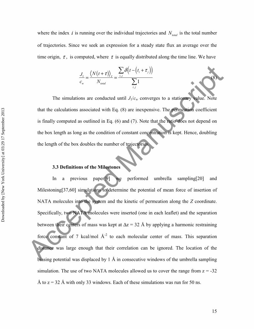
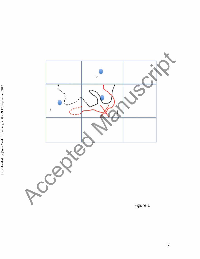
[Figure 1 near here]
Milestoning is a theory and an algorithm to compute kinetics and thermodynamics
based on atomically detailed simulations. It consists of the following steps (Figure 1): (a)
Anchor definition, (b) Definition of milestones, (c) Sampling transitions between
milestones, and (d) Solving the Milestoning equation. Each of these steps is further
discussed below:
(a) Anchor definition. Anchors are phase space points that are defined in a reduced
reaction space and provide a coarse sample for the process at hand. The set of
anchors is denoted by Yi while the set of the atomically detailed phase space
points is denoted by Xn . In the present manuscript we use only the coordinates to
define anchors. Anchors can be determined by prior thermodynamic sampling
(e.g. by replica exchange[41,42]), by reaction path calculations [43,44], or by
chemical intuition[34,45]. For example, studies of peptide folding and unfolding
in an explicit solvent use only the backbone dihedral angles of the peptide as the
coarse variables [42,46]. In the present example we use chemical intuition to
choose the variables that define the reaction space as explained in the Methods
section.
(b) Definition of milestones. Every configuration of the atomically detailed
simulation is mapped into a domain of a single anchor (or at most two) making it
possible to define a trajectory in anchor space. A transition between anchor
domains is determined by passing a milestone, a hypersurface separating the
spaces of two anchors. We denote a milestone between anchors i and j by Mij .
Accep
ted M
anus
cript
Dow
nloa
ded
by [
New
Yor
k U
nive
rsity
] at
03:
29 1
7 Se
ptem
ber
2013

9
It is the set of points that are closer to the anchors i and j compared to any other
milestone k . The distance of point Y at milestone Mij from anchor i is
d(Y ,Yi )2 = Y − Yi( )t
Y − Yi( ) + Δ2 and from anchor j is
d(Y ,Yj )2 = Y − Yj( )t
Y − Yj( ) where Δ is a constant shift (0.1 Å in the present
simulation) to avoid milestone crossing [47].
(c) Sampling transitions between milestones. In Milestoning we do not compute
atomically detailed trajectories from the reactant to the product states. Instead we
compute trajectories between milestones. Trajectories initiated at milestone Mij
are integrated forward in time until they hit for the first time another milestone
M jk . The identity of the terminating milestone and the time of termination are
recorded for further processing. In particular we are interested in the kernel
function Kij , jk t( ) which is the probability density (in time) that a trajectory started
at milestone ij will hit for the first time milestone jk exactly after time t . It is
estimated numerically as Kij , jk t( ) nij , jk t( ) nij where nij is the number of
trajectories initiated at milestone ij and nij , jk t( ) is the number of trajectories
initiated at ij that hit for the first time milestone jk exactly after time t . The
trajectories are initiated at Mij from a first hitting point distribution (FHPD
[37,47,48]), which is the probability density of phase space points that hit for the
first time milestone Mij (the last milestone that they cross previously was
different from Mij ). For complex systems the analytical form of the FHPD is not
Accep
ted M
anus
cript
Dow
nloa
ded
by [
New
Yor
k U
nive
rsity
] at
03:
29 1
7 Se
ptem
ber
2013
10
known. We approximate it by the equilibrium distribution with filtering based on
backward trajectories (Figure 1).
(d) Solving the Milestoning equation. With the kernel Kij , jk t( ) we consider the
Milestoning equation[49]
qij t( ) = pijδ t +( ) + qki t '( )Kki,ij t − t '( )dt '0
t
∫ki∑ (2)
where pij is an initial condition (the probability that the last milestone that was
crossed at time t=0 was ij ). The number of trajectories that passes milestone ij
per unit time (the flux) at time t is qij t( ) which is the vector of functions of
length of the number of milestones that we seek. The Milestoning equation is a
convolution that can be solved with Laplace transform techniques to obtain
quantities of interest [37,50]. For example, we consider the overall mean first
passage time (MFPT). It is the average first time the system hits the last milestone
f after being initiated according to the probability vector pij ≡ p( )ij
τij→ f
= p( )ijI − K( )−1 t (3)
where τij→ f
is the MFPT for the transition from milestone ij to f , I is the
identity matrix, and K is the stationary transition matrix given by
K( )ij ,km= Kij ,km t( )dt
0
∞
∫ . The matrix K is chosen such that K f ,kl = 0 ∀kl , an
absorbing boundary condition. Finally, t is a vector with the lifetimes of all the
milestones t( )ij= tKij , jk (t)dt
0
∞
∫jk∑ . We can also use the Milestoning equation to
Accep
ted M
anus
cript
Dow
nloa
ded
by [
New
Yor
k U
nive
rsity
] at
03:
29 1
7 Se
ptem
ber
2013
11
determine the stationary (time independent) fluxes qstat between the milestones.
The stationary flux is determined by the matrix equation
qstat (I − K) = 0 (4)
To obtain the stationary state we set a cyclic boundary condition.
K f ,lm = 1 lm = ij
0 otherwise
⎧⎨⎪
⎩⎪
⎫⎬⎪
⎭⎪
Finally the stationary probability and the free energy that the last milestone that
was passed is ij, is given by
pstat( )ij= qstat( )ij
t( )ij Fij = −kT log pstat( )ij
⎡⎣
⎤⎦
(5)
The stationary flux, qstat , is determined up to a multiplicative positive constant c . Hence
if q is a solution so is cq. A way of fixing the value of c is to require that the sum over all
probabilities (Eq. (5)) is equal one. However, for stationary fluxes and studies of relative
fluxes, this is not convenient. Most of the times (an exception is described below) we set
the flux at the first milestone to unity, i.e. q1 = 1.
The transitions between milestones are quantified by the stationary fluxes and
create a kinetic network. The network is analyzed to elucidate mechanisms of reaction
and the contributions of alternative reaction spaces [46]. We will use these tools to better
understand the permeation process through the membrane.
Since the most common experimental observable for membrane transport is the
permeation coefficient, P, we outline below the direct calculations of P using
Milestoning. The permeation coefficient is defined as the flux normalized (divided) by
the concentration difference in steady state conditions. The fundamental entity of
Milestoning is the flux, q, given by Eq. (4) and normalized such that the initial flux is
Accep
ted M
anus
cript
Dow
nloa
ded
by [
New
Yor
k U
nive
rsity
] at
03:
29 1
7 Se
ptem
ber
2013

12
unity. The final flux qf under stationary conditions is the permeation coefficient once
written in the proper units. We write P = J1 c( )qf where q1 = 1. The flux J1 is the
number of molecules that pass in unit area and unit time through the first milestone and c
is the concentration gradient. The first milestone is in aqueous solution (Fig. 2), which
makes it possible to estimate its entry flux from a free diffusion model.
[Place Figure 2 here]
The concentration c is the number of molecules divided by volume c=n/V. The
flux is J=n/(At) where A is a cross section of the volume and t is the time. Therefore we
have J/c=l/t. We estimate this diffusion flux with over damped Langevin dynamics in one
dimension. The only required parameter for the Langevin Eq. is the diffusion constant, D.
It is extracted from atomically detailed simulations of the permeant in aqueous solution
(see Methods).
To model P we set dual cyclic boundary conditions. The first condition (as
discussed immediately after Eq. (4)) is on the final milestone. Every molecule that makes
it to the final milestone is moved to the first milestone, i.e.
K f ,ij = 1 ij = 1
0 otherwise
⎧⎨⎪
⎩⎪
⎫⎬⎪
⎭⎪
The second adjustment is to add a solvent milestone (number 0) to which the first
membrane milestone (milestone 2) is connected. Milestone 0 has the same physical
location as milestone 1 but the velocity has an opposite direction. In milestone 1 the
velocity is pointing to the membrane and in milestone 0 it is pointing to the solvent.
Milestones 0 and 1 are a pair of directional milestones [47]. A molecule that arrives to
milestone 0 is moved with probability one to milestone 1 (Fig. 2):
Accep
ted M
anus
cript
Dow
nloa
ded
by [
New
Yor
k U
nive
rsity
] at
03:
29 1
7 Se
ptem
ber
2013
13
K0,ij = 1 ij = 1
0 otherwise
⎧⎨⎪
⎩⎪
⎫⎬⎪
⎭⎪
To summarize, the permeation coefficient is given by the following formulaes
P = ′qf (6)
where q ' f is determined by
q ' I - K( ) = 0 & q '1 = J1 cw (7)
where cw is the concentration of NATA in aqueous solution.
3. Methods
3.1 Molecular Dynamics
The starting set of configurations was taken from simulations performed previously[9].
Briefly, the simulation box contains 40 DOPC lipid molecules, 1542 water molecules and
2 NATA (N-acetyl-L-tryptophanamide) molecules. The size of the simulation cell is
37 × 37 × 75 Å, with the Z axis perpendicular to the bilayer surface. The side chain and
backbone atoms of NATA are modeled with the OPLS united-atom force field [51] and
the Berger force field [52] parameters were used for the lipid molecules. Water molecules
were represented with the SPC model [53]. Periodic boundary conditions were applied in
the three spatial directions. The long-range component of the electrostatics interaction
was calculated using the smooth Particle Mesh Ewald method [54] with a grid of
32 × 32 × 64 as implemented in the program MOIL[55] including the newest GPU
implementation of the program.[56] The real space cutoff for the electrostatics and the
van der Waals interactions was set to 9.0 Å. In all the simulations we constrain water
bond lengths and angle with a matrix version[57] of the SHAKE algorithm[58], and r-
Accep
ted M
anus
cript
Dow
nloa
ded
by [
New
Yor
k U
nive
rsity
] at
03:
29 1
7 Se
ptem
ber
2013

14
RESPA[59] was used to have a dual time stepping; the reciprocal-space component of the
Ewald sum was evaluated every 4 fs and the rest of the forces were evaluated every 1 fs.
3.2 Initial Flux
To compute the initial flux, J1, we first estimated the diffusion constant of NATA
in aqueous solution. We simulated NATA in a box of water of 64x64x64 Å3 for a period
of 300 picoseconds (ps) (trajectory length of 300 ps is probably more than what was
required). The time step was 0.5ps, and the grid for Particle Meshed Ewald was 643. We
calculated the diffusion coefficient from the relationship 2Dt = x2 .
The diffusion constant is used in over-damped Langevin simulations to estimate
the incoming flux to the first milestone. The simulations are conducted in a one-
dimensional box 0, l[ ] with a test boundary at l . Initial coordinates in the box are
distributed uniformly in the interval 0, l[ ]and trajectories are conducted until they “hit” l.
Their time is recorded and they are terminated. Displacements for Brownian trajectories
are generated from a normal distribution with zero mean and variance of 2D ⋅δt where
δt is the time step. Trajectories are conducted to estimate J1/cw as np / n at the absorbing
boundary where np is the number of trajectories that hit l per unit time under constant
flux conditions and n is the total number of trajectories.
More formally, we define the ratio of the total number of trajectories that hit l at
time t normalized by the total number of trajectories as N t( ) / Ntotal = δ t − ti( )i∑⎡⎣⎢
⎤
⎦⎥ / Ntotal
Accep
ted M
anus
cript
Dow
nloa
ded
by [
New
Yor
k U
nive
rsity
] at
03:
29 1
7 Se
ptem
ber
2013
15
where the index i is running over the individual trajectories and Ntotal is the total number
of trajectories. Since we seek an expression for a steady state flux an average over the
time origin, τ , is computed, where τ is equally distributed along the time line. We have
J1
cw
=N t + τ( ) τ
Ntotal
=δ t − ti + τ j( )( )
i, j∑
1i , j∑
(8)
The simulations are conducted until J1/cw converges to a stationary value. Note
that the calculations associated with Eq. (8) are inexpensive. The permeation coefficient
is finally computed as outlined in Eq. (6) and (7). Note that the ratio does not depend on
the box length as long as the condition of constant concentration is kept. Hence, doubling
the length of the box doubles the number of trajectories.
3.3 Definitions of the Milestones
In a previous paper[9] we performed umbrella sampling[20] and
Milestoning[37,60] simulations to determine the potential of mean force of insertion of
NATA molecules into the system and the kinetic of permeation along the Z coordinate.
Specifically, two NATA molecules were inserted (one in each leaflet) and the separation
between their centers of mass was kept at Δz = 32 Å by applying a harmonic restraining
force constant of 7 kcal/mol Å-2 to each molecular center of mass. This separation
distance was large enough that their correlation can be ignored. The location of the
biasing potential was displaced by 1 Å in consecutive windows of the umbrella sampling
simulation. The use of two NATA molecules allowed us to cover the range from z = -32
Å to z = 32 Å with only 33 windows. Each of these simulations was run for 50 ns.
Accep
ted M
anus
cript
Dow
nloa
ded
by [
New
Yor
k U
nive
rsity
] at
03:
29 1
7 Se
ptem
ber
2013

16
Here we go beyond the one-dimensional permeation coordinate used previously.
Starting configurations for the current work were selected from the last 5 ns
configurations saved of the previous 50 ns simulations. We sample structures at fixed
values of the normal to the membrane, from z = -30 Å to z = 30 Å with a 2 Å separation
between them. We also added a new coarse variable that measures molecular orientation.
Specifically, let us denote as rorient = rback − rside the vector connecting the two centers of
mass of the backbone, rback, and the side chain, rside. Then, the second coarse-grained
coordinate that we use to assess the molecular orientation is
zorient = rorientt ⋅ ez
where ez is a unit vector along the Z axis (the normal to the membrane plane).
For a given value of z we sampled seven different values of the orientational
coordinate ranging from zorient = −6 Å to zorient = 6 Å with a 2 Å separation. The
combination of z and zorient values we are considering gives a total of 217 different
anchors, evenly distributed in the two-dimensional space defined by these two
coordinates (those anchors are shown in Figure 3).
From this set of anchors we constructed a set of 1512 milestones (interfaces
dividing domains associated with these anchors). These sets of milestones were
constructed such that every anchor i connects directly with 8 adjacent anchors, and the
interface corresponding to the transition i → j is different from the interface associated
with the transition j → i (See 2.b). The anchors at the borders of the z and zorient two-
Accep
ted M
anus
cript
Dow
nloa
ded
by [
New
Yor
k U
nive
rsity
] at
03:
29 1
7 Se
ptem
ber
2013

17
dimensional space are connected with five other anchors (or only three if the anchors are
at the corners).
3.4 First Hitting Point Distribution
Having defined this set of milestones, we approximate the FHPD distribution by
sampling configurations with Boltzmann weights (canonical ensemble) that are
harmonically restrained to the neighborhood of each of the milestones, as described
in[9,47]. Initial configurations for this sampling were taken from the last 5 ns of the 50 ns
restrained simulations performed previously. The canonically restrained distribution in
the two-dimensional milestones was generated by computing 7 ns of iso-kinetic
trajectories in each of the milestones that was shown to yield the canonical
distribution[61]. The two NATA molecules were constrained in these simulations. In
total, we performed 1512/2=756 of such simulations since we exploit the presence of two
permeating NATA molecules in a single membrane. The 7 ns timescale was enough to
provide a thorough sampling on these more spatially localized milestones. From these
sampling simulations about 1000 configurations were saved for the next step of
calculations in which we filter from the ensemble of canonically sampled structures, the
first hitting point distribution [37,47,48].
Specifically, starting from the configurations saved in the sampling step we
removed the harmonic constraint in one of the two NATA molecules and performed
“backward” MD simulations in the system (the harmonic constraint was maintained on
the second molecule). During the simulation we check if the unconstrained solute hits a
Accep
ted M
anus
cript
Dow
nloa
ded
by [
New
Yor
k U
nive
rsity
] at
03:
29 1
7 Se
ptem
ber
2013

18
neighboring milestone before hitting the initial milestone (Figure 1). If this was the case,
the initial configuration and velocities (drawn according to a Maxwell distribution at 300
K) are considered a first hitting point for this current milestone and the phase space data
is saved for the final step of the Milestoning procedure. If during this backward
simulation the unconstrained permeant hits the starting milestone first before hitting a
neighboring one, then we stop this trajectory and discard this phase space point. This
process was repeated until we collected from 100 to 480 first hitting point configurations
for each milestone.
3.5 Computing the Transition Kernel
In the final step, we performed unconstrained simulations starting with the first
hitting points obtained from the previous step. In this case, we performed “forward” MD
simulations by reversing the sign of the initial set of velocities saved in the previous step.
The run is stopped when a neighboring milestone is hit regardless of whether the initial
milestone is crossed or not during the simulation. The information saved in this step is the
identity of the neighboring milestone that is hit and the time it took for this to happen. We
extract the matrix K( )ij , jk and the vector of the lifetimes of the milestones - t( )ij
. The
matrix and the vector are used in the Milestoning calculation outlined in Eq. (2)-(7).
Overall we have run a total of 119,819 trajectories with accumulated simulation
time of 5.2 microseconds. The average time per trajectory was 43 picoseconds. Hence the
simulations exploit parallelization very efficiently since the trajectories are independent.
3.6 MaxFlux
Accep
ted M
anus
cript
Dow
nloa
ded
by [
New
Yor
k U
nive
rsity
] at
03:
29 1
7 Se
ptem
ber
2013

19
The calculation of kinetic networks in general and the present investigation in particular
can be complex and difficult to analyze. A useful interpretation tool is the extraction of
reaction coordinates and specific mechanisms. While “best” reaction coordinate is
debatable[39,62-68], a useful choice would be a pathway that carries the maximum flux
(MaxFlux[69]) of trajectories from reactants (one side of the membrane) to products (the
other side of the membrane) and therefore makes the most significant contribution to the
reaction. In the present network, the nodes are the anchors and the weight of the edges
connecting two anchors i and j are the net fluxes wij = qij − qji where qij and qji are the
stationary fluxes going from anchor domains i → j and from anchors j → i,
respectively[37]. Those fluxes are obtained by solving the Milestoning equations (section
2.d). Given the net fluxes the MaxFlux path on the network is computed using the
following algorithm: [37]
1. Find the edge with the smallest weight on the graph that corresponds to the
milestone with the smallest flux. Mark that edge for elimination.
2. Check if there is still a path connecting the initial and final state after removing
the edge marked in the previous step. If there is still a path, then remove the edge
from the graph. If there is no such a path, then this edge is essential for the
MaxFlux path; thus it is kept, but is not considered any longer for removal in step
1.
3. Return to step 1 until a continuous path from reactant to product was determined.
The collection of all edges that remain after running the algorithm is the MaxFlux
path connecting the initial and final states in the discrete representation of the process
Accep
ted M
anus
cript
Dow
nloa
ded
by [
New
Yor
k U
nive
rsity
] at
03:
29 1
7 Se
ptem
ber
2013

20
given by the Milestoning calculation. In this discrete representation a transition state is
the edge in the MaxFlux path with the smallest weight (flux). A second best MaxFlux
path can be obtained by eliminating the transition state (edge along the path with minimal
weight) found in the first MaxFlux path since our focus is typically on the bottleneck or
the edge with the lowest flux. A third best MaxFlux path is obtained by further
eliminating the transition state of the second best MaxFlux path, and the process can be
repeated to obtain additional paths.
5. Results
5.1. Free energy and Permeation Pathways
The equilibrium probability distribution for the system was obtained by solving the
Milestoning equation (Equation (5)). The corresponding 2D free energy surface as a
function of the membrane axis Z and the orientational direction is shown in Figures 3 and
4. Figure 3 shows the probability distributions obtained by solving the Milestoning
equations for the whole membrane, and Figure 4 shows an average of the results over the
two halves of the membrane permeation in Figure 3, i.e. enforcing the expected
symmetry. In the most populated regions at the interface between the polar and
hydrophobic groups of the membrane (at about Z = 15 Å), the permeant favors an
orientation in which most of its backbone atoms point to the closest water phase
(orientational angle larger than 90° on the left side and smaller than 90° on the right side).
There is an increase of free energy when the permeant moves from that region to the
center of the bilayer. This barrier region is narrower when the orientational angle is
between 65° and 115° (Figure 4). This equilibrium view of the permeation process
Accep
ted M
anus
cript
Dow
nloa
ded
by [
New
Yor
k U
nive
rsity
] at
03:
29 1
7 Se
ptem
ber
2013

21
suggests that at the center of the membrane NATA prefers an orientation where the
indole ring and polar atoms are perpendicular to the membrane normal. More tilted
orientations at the center of the bilayer are less beneficial for transmembrane diffusion.
[Figure 4 near here]
[Figure 5 near here]
To compare with previous free energy profile estimates we sum the probabilities
along the orientation coordinate and took the logarithm to obtain a one dimensional free
energy profile along the membrane axis Z. Figure 5 shows the current results for NATA
permeation compared with our previous Milestoning estimates using a one dimensional
reaction coordinate, and results using the solubility diffusion model (SDM). Qualitatively
they all show a preferential location of NATA to be at the interface between the
hydrophobic tail and the glycerol region of the lipids. A barrier is present at the center of
the bilayer with a relative free energy in the range between 16.5 to 20 kcal/mol. The
figure also displays the free energy profile for the indole ring of tryptophan. This less
hydrophilic permeant compared to NATA shows a smaller barrier at the center. Note the
lower variance of the SDM results. We should keep in mind however, that the SDM is a
simpler equilibrium model that is based on overdamped Langevin model throughout the
process. Its simplicity is of course an advantage, and makes the estimate of a fewer
parameters more stable statistically. However, it is not clear if the model is correct
dynamically (neglect of memory effects). It is also not obvious how to use a SDM or a
similar model to incorporate other HSVs. The calculation of diffusion constant and the
MFPT theory for diffusion in high dimension is still under investigation [70] while the
Accep
ted M
anus
cript
Dow
nloa
ded
by [
New
Yor
k U
nive
rsity
] at
03:
29 1
7 Se
ptem
ber
2013

22
Milestoning algorithm is straightforward even in high dimension and for arbitrary
(classical) dynamics. We therefore discuss in details only the Milestoning results.
[Figure 6 near here]
5.2. Mean first passage time
The mean first passage times for permeation of NATA from the water phase to the center
of the bilayer were computed using Eq. (3) and the results are shown in Table 1. The
permeation time ranges from 5 minutes to about 2 hours while the experimental times are
of order of a few hours[9]. The previous one- dimensional results using Milestoning
showed a larger value for one of the layers and a larger discrepancy between the timing
of the two layers. The estimate using the solubility-diffusion equations is slightly faster
than our current results. But the results for the three methods are similar. Clearly the
slower permeation for the positive side of the membrane repeats in all simulations. As we
discussed earlier for the free energy, the SDM shows smaller variance that is likely
associated with a simpler model. Milestoning is more accurate in principle and more
easily extendable to higher dimensions.
[Table 1 near here]
5.3. MaxFlux results
Figure 6 shows the Maxflux paths obtained by applying the Maxflux algorithm described
in the method section to the two dimensional network of anchors in the Z and Z’ space.
The figure displays the seven best Maxflux paths that are represented in the figure by the
collection of edges that remain after solving the algorithm. The difference of the
Accep
ted M
anus
cript
Dow
nloa
ded
by [
New
Yor
k U
nive
rsity
] at
03:
29 1
7 Se
ptem
ber
2013

23
magnitude of the flow between the first and seventh best MaxFlux paths is a factor of ten,
so many of these paths should be relevant for the permeation process. The different paths
only differ in the central region of the membrane, in which an orientational flip-flop
occurs and the permeant leaves one leaflet and enters the second one. For all the paths
shown when the permeant moves from z= -8 Å to z = 14 Å, the orientational angle
changes by 90 degrees from 135° to 45°. At the membrane center (z = 0 Å) four anchors
are involved in the paths with orientational angles of 69°, 90°, 111° and 135°. For the
path with maximum flux (represented with the black segment in the figure) the
orientational flip-flop only occurs after the permeant has crossed through the membrane
center. We computed the best MaxFlux for trajectories moving in the opposite direction
and found similar results: that the permeant starts to rotate only after it has passed the
center of the bilayer. The transition state of all of the MaxFlux paths (colored with
different shades of gray) involves anchors at z = 0 Å (all seven of them), z = 2 Å (five of
them) and z = -2 Å (one of them), so for 5 paths the transition state is observed after the
permeant has just crossed the center of the membrane.
[Figure 7 near here]
5.4 Backbone torsion angles
Figure 7 shows representative variations of the backbone dihedral angles of NATA
molecules while moving inside the membrane. When the molecule is deeper inside the
negative Z layer (left panels, a and c) it tends to obtain an extended conformation while it
is more helical in areas of the bilayer closer to the water phase (e). The right panel
(positive Z layer) shows a different behavior close to the membrane center with a more
Accep
ted M
anus
cript
Dow
nloa
ded
by [
New
Yor
k U
nive
rsity
] at
03:
29 1
7 Se
ptem
ber
2013

24
helical conformation. The next figure (Figure 8) shows the potential of mean force along
the dihedral ψ angle for fixed Z values. An extended conformation at small absolute Z
values is more stable according to these calculations.
[Figure 8 near here]
[Figure 9 near here]
The negative Z layer explored the extended conformation but the positive layer
significantly less. We also observed that the latter layer showed more water molecules
coming closer to the center than the negative layer (Figure 8). The difference between
the helical and the extended chain configuration is of order of 1 kcal/mol when NATA is
closer to the membrane center. If we assume that the energy difference between
conformers reduces the overall barrier by the same amount, we expect a transition
speedup of about exp(1/0.6)=5.3 at 300 K. This factor is lower than the observed speedup
of ~20 in the permeation times (Table 1). Hence the conformational transition does not
provide the complete answer to the permeation asymmetry of the two layers.
[Figure 9 near here]
5.5 Permeation coefficient
We computed the permeation coefficient as described in the Milestoning and Method
sections. The diffusion constant, D , of NATA in aqueous solution was estimated from
the relations 2Dt = x2 to be1.6 ⋅10−5 cm2 / s . The estimate of J1 / cw based on one
dimensional diffusion model (Eq. (8)) gives J1 / cw = 251 cm / sec.
Accep
ted M
anus
cript
Dow
nloa
ded
by [
New
Yor
k U
nive
rsity
] at
03:
29 1
7 Se
ptem
ber
2013

25
The Milestoning calculation provides two permeation coefficients estimated for each of
the two halves of the membrane. The two results are used to grasp the values of the error
bars for P. The permeability coefficient obtained from the Milestoning calculations are
8.8 ⋅10−10 cm / s and 4.3 ⋅10−11cm / s for the first and second membrane halves
respectively. The difference is quite large and suggests that we can determine the
permeability coefficient only up to a factor of 20. A similar accuracy is obtained for the
SDM in which the corresponding values are 1.91 ⋅10−10 cm / s and 2.63 ⋅10−11cm / s for
both sides of the membrane. The difference here is smaller (a factor of about 10) but still
significant and is within the difference between the two technologies. Given that the
computational technologies are very different we find the agreement quite satisfactory.
Unfortunately there are no measurements for the permeation coefficient of NATA.
However, we reported in section 5.2 (and in reference [9]) a comparison between
experimental measurements and simulations of the first passage time.
6. Discussions and conclusions
As discussed in the Introduction atomically detailed simulations of molecular
permeation frequently use a model that is inherently one-dimensional. The model
considers explicitly only the center of mass of the permeant and its projection along the
normal to the membrane, Z. This choice implies that all other degrees of freedom are fast
to relax on the Molecular Dynamics time scale and are in local equilibrium with the fixed
value of Z. If this is not the case and there are Hidden Slow Variables (HSV) in the
system then computations of averages will show high variance and will not be accurate,
Accep
ted M
anus
cript
Dow
nloa
ded
by [
New
Yor
k U
nive
rsity
] at
03:
29 1
7 Se
ptem
ber
2013

26
even if the time scale of the HSV is much shorter than the time scale of the transition
along Z. We expect significant deviations from one-dimensional picture for larger and
more complex permeant, such as the system studied here.
To determine the presence of additional HSV (besides Z) MD simulations are
conducted independently for each of the membrane layers. In equilibrium the properties
of each half must be the same. If the two MD averages show significant deviations then
there must be HSV in the system that are sampled differently at each half. The computed
MFPT for NATA permeation differed for both sides by a factor of about 150 in our
previous 1D Milestoning[9]. We therefore searched for plausible slow coarse variables
that may influence the rate.
If we identify these variables correctly then we could enhanced their sampling in
a similar fashion to what we have done for the Z coordinate, by enhanced sampling
techniques such us umbrella sampling [20], metadynamics [71], TAMD [31], TAMC [32]
and Milestoning [42]. The advantage of using Milestoning in higher dimension is that the
kinetic calculations are straightforward. This is not the case for SDM and variants since
Jacobian factors and diffusion tensors require additional considerations. The
enhancement of sampling should prevent dependence on initial conditions.
How do we identify these coarse variables? In the present manuscript we consider
two options. We evaluate one of them in full (orientation) and for the second (backbone
dihedral angles) we estimate the free energy landscape. We assumed that molecular
Accep
ted M
anus
cript
Dow
nloa
ded
by [
New
Yor
k U
nive
rsity
] at
03:
29 1
7 Se
ptem
ber
2013

27
orientation was a HSV and computed two dimensional free energy landscape and MFPT
using Milestoning. The kinetic asymmetry of the halves was reduced from a factor of 150
(1D Milestoning), to about 20 (2D Milestoning). Although this 7.5 reduction of the
MFPT asymmetry indicates that the orientation is a HSV, the fact that that the asymmetry
did not vanish suggests that it is not the only HSV that contributes to the differences
between the MFPTs. We also examined the energy landscape of the peptide
conformational transition at different depths of the membrane. While some small
differences were observed for the transition between the helix and the extended chain (of
order of 1 kcal/mole) they are probably not sufficient to explain the factor of 20 of
difference in MFPT passing each of the layers. Hence, our investigations, while
providing considerable insight into the mechanism and pathways of the permeation, did
not identify quantitatively all the sources that contribute to the permeation rate of NATA
and that can explain the differences between the membrane layers.
We finally speculate on other candidates to HSVs that can be investigated in
future work. For example, we observed in our simulations a different number of
permeating water molecules that attach themselves to the translocating peptide. A larger
number of water molecules is found in the layer in which the peptide permeates more
slowly. It is not obvious if the water permeation is associated with the conformational
change of the peptide. Hence water presence and peptide conformation may be strongly
coupled and not independent, a possibility that we will explore in the future. Yet another
possibility is that the phospholipid conformations and packing are different at each leaflet
and the relaxation from one packing state to another is long on the MD time scale for
Accep
ted M
anus
cript
Dow
nloa
ded
by [
New
Yor
k U
nive
rsity
] at
03:
29 1
7 Se
ptem
ber
2013

28
each milestone slice. For each of the milestone we consider 7 ns in the two dimensional
milestones and 50 ns for the one dimensional milestones calculated previously[9].
While the present manuscript is at least partially negative in the sense that it did
not quantify all the factors that affect the permeation rate of NATA through a DOPC
membrane we hope that it will help point out key challenges in membrane simulations
and provide guidelines when quantitative prediction (and estimation of error bars) of
permeation can be made.
Acknowledgement
This research was supported by NIH grant GM59796 and Welch grant F-1783 to RE.
The authors acknowledge the Texas Advanced Computing Center (TACC) at The
University of Texas at Austin for providing HPC resources that have contributed to the
research results reported within this paper. URL: http://www.tacc.utexas.edu
Accep
ted M
anus
cript
Dow
nloa
ded
by [
New
Yor
k U
nive
rsity
] at
03:
29 1
7 Se
ptem
ber
2013

29
References
[1]D. Bassolinoklimas, H. E. Alper, and T. R. Stouch, J. Am. Chem. Soc. 117 (14), 4118
(1995).
[2]S. J. Marrink and H. J. C. Berendsen, J. Phys. Chem. 100 (41), 16729 (1996).
[3]S. J. Marrink and H. J. C. Berendsen, J. Phys. Chem. 98 (15), 4155 (1994).
[4]C. Wei and A. Pohorille, J. Phys. Chem. B 115, 3681 (2011).
[5]M. A. Wilson and A. Pohorille, J. Am. Chem. Soc. 118 (28), 6580 (1996).
[6]A. C. Chakrabarti and D. W. Deamer, J. of Mol. Evol. 39 (1), 1 (1994).
[7]A. C. Chakrabarti and D. W. Deamer, Biochim. Biophys. Acta 1111 (2), 171 (1992).
[8]D. W. Deamer and J. Bramhall, Chem. Phys. Lipids 40 (2-4), 167 (1986).
[9]A. E. Cardenas, G. S. Jas, K. Y. DeLeon, W. A. Hegefeld, K. Kuczera, and R. Elber, J.
Phys. Chem. B 116 (9), 2739 (2012).
[10]J. Sikkema, J. A. M. Debont, and B. Poolman, Microbiol. Rev. 59 (2), 201 (1995).
[11]P. Lampi, J. Tuomisto, T. Hakulinen, and E. Pukkala, Scand. J. Work Env. Hea. 34
(3), 230 (2008).
[12]A. L. Plant, D. M. Benson, and L. C. Smith, J. Cell Biol. 100 (4), 1295 (1985).
[13]A. L. Plant, H. J. Pownall, and L. C. Smith, Chem. Biol. Interact. 44 (3), 237 (1983).
[14]C. Kalyanaraman and M. P. Jacobson, J. Comp. Aid. Mol. Des. 21 (12), 675 (2007).
[15]T. X. Xiang and B. D. Anderson, Adv. Drug Deliver. Rev. 58 (12-13), 1357 (2006).
[16]M. Orsi and J. W. Essex, Soft Matter 6 (16), 3797 (2010).
[17]H. E. Alper and T. R. Stouch, J. Phys. Chem. 99 (15), 5724 (1995).
[18]P. Kuhn, K. Eyer, S. Allner, D. Lombardi, and P. S. Dittrich, Anal. Chem. 83 (23),
8877 (2011).
[19]C. Y. Cheng, O. J. G. M. Goor, and S. Han, Anal. Chem. 84 (21), 8936 (2012).
[20]G. N. Patey and J. P. Valleau, Chem. Phys. Lett. 21 (2), 297 (1973).
[21]E. A. Carter, G. Ciccotti, J. T. Hynes, and R. Kapral, Chem. Phys. Lett. 156 (5), 472
(1989).
[22]A. Pohorille, P. Cieplak, and M. A. Wilson, Chem. Phys. 204 (2-3), 337 (1996).
[23]P. Jedlovszky and M. Mezei, J. Am. Chem. Soc. 122 (21), 5125 (2000).
Accep
ted M
anus
cript
Dow
nloa
ded
by [
New
Yor
k U
nive
rsity
] at
03:
29 1
7 Se
ptem
ber
2013

30
[24]D. Bemporad, J. W. Essex, and C. Luttmann, J. Phys. Chem. B 108 (15), 4875
(2004).
[25]A. C. V. Johansson and E. Lindahl, Proteins: Struct., Funct., Bioinf. 70 (4), 1332
(2008).
[26]A. Grossfield and T. B. Woolf, Langmuir 18 (1), 198 (2002).
[27]K. E. Norman and H. Nymeyer, Biophys. J. 91 (6), 2046 (2006).
[28]JL. MacCallum and DP. Tieleman, Interactions between small molecules and lipid
bilayers, edited by DJ Benos, Simon, SA (Elsevier, Amsterdam, 2008).
[29]J. L. MacCallum, W. F. D. Bennett, and D. P. Tieleman, Biophys. J. 94 (9), 3393
(2008).
[30]J. Ulander and A. D. J. Haymet, Biophys. J. 85 (6), 3475 (2003).
[31]L. Maragliano and E. Vanden-Eijnden, Chem. Phys. Lett. 426 (1-3), 168 (2006).
[32]G. Ciccotti and S. Meloni, Phys. Chem. Chem. Phys. 13 (13), 5952 (2011).
[33]Alessandro Laio and Michele Parrinello, Proc. Nat. Acad. Sci. U. S. A. 99 (20),
12562 (2002).
[34]S. Kreuzer and R. Elber, Biophys. J. 105 (4), 951 (2013).
[35]J. E. Straub and D. Thirumalai, Proc. Nat. Acad. Sci. U. S. A. 90 (3), 809 (1993).
[36]F. X. Contreras, L. Sanchez-Magraner, A. Alonso, and F. M. Goni, Febs Lett. 584
(9), 1779 (2010).
[37]S. Kirmizialtin and R. Elber, J. Phys. Chem. A 115 (23), 6137 (2011).
[38]S. Jo, H. A. Rui, J. B. Lim, J. B. Klauda, and W. Im, J. Phys. Chem. B 114 (42),
13342 (2010).
[39]W. E., W. Q. Ren, and E. Vanden-Eijnden, J. Phys. Chem. B 109 (14), 6688 (2005).
[40]Z. Ghaemi, M. Minozzi, P. Carloni, and A. Laio, J. Phys. Chem. B 116 (29), 8714
(2012).
[41]D. J. Earl and M. W. Deem, Phys. Chem. Chem. Phys. 7 (23), 3910 (2005).
[42]G. S. Jas, W. A. Hegefeld, P. Majek, K. Kuczera, and R. Elber, J. Phys. Chem. B 116
(23), 6598 (2012).
[43]R. Elber, Biophys. J. 92 (9), L85 (2007).
[44]S. Kirmizialtin, V. Nguyen, K. A. Johnson, and R. Elber, Structure 20 (4), 618
(2012).
Accep
ted M
anus
cript
Dow
nloa
ded
by [
New
Yor
k U
nive
rsity
] at
03:
29 1
7 Se
ptem
ber
2013

31
[45]SM. Kreuzer and R. Elber, J. Chem. Phys. 139 (2013).
[46]S. M. Kreuzer, R. Elber, and T. J. Moon, J. Phys. Chem. B 116 (29), 8662 (2012).
[47]P. Majek and R. Elber, J. Chem. Theory Comput. 6 (6), 1805 (2010).
[48]Eric Vanden Eijnden, Maddalena Venturoli, G. Ciccotti, and R. Elber, J. Chem. Phys.
129 (17), 174102 (2008).
[49]A. K. Faradjian and R. Elber, J. Chem. Phys. 120 (23), 10880 (2004).
[50]D. Shalloway and A. K. Faradjian, J. Chem. Phys. 124 (5), 054112 (2006).
[51]W. L. Jorgensen and J. Tiradorives, J. Am. Chem. Soc. 110 (6), 1657 (1988).
[52]O. Berger, O. Edholm, and F. Jahnig, Biophys. J. 72 (5), 2002 (1997).
[53]H. J. C. Berendsen, J. R. Grigera, and T. P. Straatsma, J. Phys. Chem. 91 (24), 6269
(1987).
[54]T. Darden, D. York, and L. Pedersen, J. Chem. Phys. 98 (12), 10089 (1993).
[55]R. Elber, A. Roitberg, C. Simmerling, R. Goldstein, H. Y. Li, G. Verkhivker, C.
Keasar, J. Zhang, and A. Ulitsky, Comput. Phys. Commun. 91 (1-3), 159 (1995).
[56]A.P. Ruymgaart, A.E. Cardenas, and R. Elber, J. Chem. Theory Comput. 7 (2011).
[57]Y. Weinbach and R. Elber, J. Comput. Phys. 209 (1), 193 (2005).
[58]J. P. Ryckaert, G. Ciccotti, and H. J. C. Berendsen, J. Comput. Phys. 23 (3), 327
(1977).
[59]M. Tuckerman, B. J. Berne, and G. J. Martyna, J. Chem. Phys. 97 (3), 1990 (1992).
[60]A. M. A. West, R. Elber, and D. Shalloway, J. Chem. Phys. 126 (14), 145104 (2007).
[61]J.B. Abrams, Tuckrman, M.E., Martyna, G.,J.,, Computer simulations in condensed
matter: From materials to chemical biology. Vol 1, edited by M. Ferrario,
Ciccotti, G., Biner, K. (Springer, Berin, 2006).
[62]A. Ulitsky and R. Elber, J. Chem. Phys. 92 (2), 1510 (1990).
[63]R. Olender and R. Elber, Theochem-J. Mol. Struct. 398, 63 (1997).
[64]R. Elber and D. Shalloway, J. Chem. Phys. 112 (13), 5539 (2000).
[65]P. Faccioli, M. Sega, F. Pederiva, and H. Orland, Phys. Rev. Lett. 97 (10), 108101
(2006).
[66]W. Lechner, C. Dellago, and P. G. Bolhuis, J. Chem. Phys. 135 (15) (2011).
[67]L. Maragliano and E. Vanden-Eijnden, Chem. Phys. Lett. 446 (1-3), 182 (2007).
[68]W. N. E, W. Q. Ren, and E. Vanden-Eijnden, Phys. Rev. B 66 (5), 4 (2002).
Accep
ted M
anus
cript
Dow
nloa
ded
by [
New
Yor
k U
nive
rsity
] at
03:
29 1
7 Se
ptem
ber
2013

32
[69]S. H. Huo and J. E. Straub, J. Chem. Phys. 107 (13), 5000 (1997).
[70]A. Berezhkovskii and A. Szabo, J. Chem. Phys. 135 (7) (2011).
[71]Y. Crespo, F. Marinelli, F. Pietrucci, and A. Laio, Phys. Rev. E 81 (5) (2010).
Figure captions:
Figure 1. A schematic representation of the Milestoning algorithm. The blue filled
circles denote anchors and the straight blue lines represent the milestones (interfaces)
separating the different anchor domains . In Milestoning we estimate the probability that
a trajectory initiated at a milestone ij will hit for the first time another milestone jk at time
t. We estimate this probability by running a large number of trajectories from ij and
record the number of and times of trajectories that hit milestone jk for the first time. The
black and red curves are trajectories initiated at milestone ij and terminated at milestone
jk. The dashed lines denote time-backward trajectories and are used to check if the initial
phase space points are sampled from a first hitting distribution. The black trajectory is
acceptable (the backward trajectory reached a different milestone before hitting again the
initial milestone) while the red trajectory is not (it returns to the initiating milestone,
before hitting another milestone). See Method and reference [37] for more details.
Accep
ted M
anus
cript
Dow
nloa
ded
by [
New
Yor
k U
nive
rsity
] at
03:
29 1
7 Se
ptem
ber
2013
33
Accep
ted M
anus
cript
Dow
nloa
ded
by [
New
Yor
k U
nive
rsity
] at
03:
29 1
7 Se
ptem
ber
2013

34
Figure 2. A schematic representation of the system used to compute the permeation
coefficient. We used one-dimensional set up of milestones denoted by blue lines in the
figure. We also used cyclic boundary conditions in which trajectories that reach the last
milestone qf are returned to the first milestone q1 with probability one. Trajectories that
return from milestone q2 to milestone q0 are also returned with probability one to q1. See
text for more details.
Accep
ted M
anus
cript
Dow
nloa
ded
by [
New
Yor
k U
nive
rsity
] at
03:
29 1
7 Se
ptem
ber
2013

35
Figure 3. The two-dimensional free energy surface for the permeation of NATA through
a DOPC bilayer, along the membrane axis Z and the orientational coordinate of NATA
(expressed as an angle in this and the next figures). The free energy landscape is a
solution of the Milestoning equation, Eq. (5). The energy units are in kcal/mole and the
color code is provided in the sidebar (blue corresponds to more probable configurations
of the system, and red to less populated). The figure also shows (brown dots) the location
of the anchors used in the simulation. If the permeant orientation were the HSV that
influences the asymmetry in the free energy landscape our explicit enhanced sampling of
the orientation would yield a symmetric graph with respect to the membrane center. This
is not the case. The minimum on the right is deeper and the permeation on the left side is
faster. The difference in well depths of about 3 kcal/mol can explain the difference in the
kinetics of the two halves. See text for more details.
Accep
ted M
anus
cript
Dow
nloa
ded
by [
New
Yor
k U
nive
rsity
] at
03:
29 1
7 Se
ptem
ber
2013

36
Accep
ted M
anus
cript
Dow
nloa
ded
by [
New
Yor
k U
nive
rsity
] at
03:
29 1
7 Se
ptem
ber
2013

37
Figure 4. The two-dimensional free energy surface for the permeation of NATA through
a DOPC bilayer, along the membrane axis z and the orientational coordinate of NATA
described in the text. At the center of the membrane z = 0 Å. An orientation of 90°
corresponds to a NATA molecule being perpendicular to the membrane axis. In the
figure, blue corresponds to more probable configurations of the system, and red to less
populated. The plot is a symmetric average of the results of Fig. 2.
Accep
ted M
anus
cript
Dow
nloa
ded
by [
New
Yor
k U
nive
rsity
] at
03:
29 1
7 Se
ptem
ber
2013

38
Accep
ted M
anus
cript
Dow
nloa
ded
by [
New
Yor
k U
nive
rsity
] at
03:
29 1
7 Se
ptem
ber
2013

39
Figure 5. One-dimensional free energy profile for the permeation of NATA and an indole
ring. The current results using a two dimensional description of the permeation process
and then reducing the profile to one dimension are shown in the solid line. Previous one-
dimensional results using Milestoning are shown with dash line and the solubility
diffusion model is presented with square symbol. Also shown is the permeation free
energy profile for tryptophan side chain with x symbol.
Accep
ted M
anus
cript
Dow
nloa
ded
by [
New
Yor
k U
nive
rsity
] at
03:
29 1
7 Se
ptem
ber
2013

40
Accep
ted M
anus
cript
Dow
nloa
ded
by [
New
Yor
k U
nive
rsity
] at
03:
29 1
7 Se
ptem
ber
2013

41
Figure 6. The seven best MaxFlux paths for permeation of NATA through the membrane.
Note the overall curved shape of the path that tends to visit the minima on the left and on
the right when crossing the central barrier. The transition state for each of the paths are
colored with different grays (the fastest the transition the darkest the gray color). The
paths are not symmetric with respect to the center due to discretization (grid) errors.
Accep
ted M
anus
cript
Dow
nloa
ded
by [
New
Yor
k U
nive
rsity
] at
03:
29 1
7 Se
ptem
ber
2013

42
Accep
ted M
anus
cript
Dow
nloa
ded
by [
New
Yor
k U
nive
rsity
] at
03:
29 1
7 Se
ptem
ber
2013

43
Figure 7. Sampling of the backbone dihedral angles φ,ψ( ) of NATA for different
locations along the Z axis. The left side panels correspond to the layer with negative
values of Z and the right side to positive values. (a) and (b) |Z| = 0 Å, (c) and (d) |Z| = 4
Å, (e) and (f) |Z| = 15 Å, (g) and (h) |Z| = 30 Å. Positive Z values correspond to slower
permeation.
Accep
ted M
anus
cript
Dow
nloa
ded
by [
New
Yor
k U
nive
rsity
] at
03:
29 1
7 Se
ptem
ber
2013

44
Accep
ted M
anus
cript
Dow
nloa
ded
by [
New
Yor
k U
nive
rsity
] at
03:
29 1
7 Se
ptem
ber
2013

45
Figure 8. Potential of mean force for NATA along the dihedral angle ψ for three different
locations inside the membrane (z = 0 Å, z = |5| Å and z = |15|). The potential of mean
force was computed with no presence of permeating water molecules at the membrane
center (which sometimes are seen to follow NATA towards the center of the
membrane[9]).
Accep
ted M
anus
cript
Dow
nloa
ded
by [
New
Yor
k U
nive
rsity
] at
03:
29 1
7 Se
ptem
ber
2013

46
Accep
ted M
anus
cript
Dow
nloa
ded
by [
New
Yor
k U
nive
rsity
] at
03:
29 1
7 Se
ptem
ber
2013

47
Figure 9. Average number of water molecules that penetrate inside the hydrophobic core
of the membrane (within 10 Å from the membrane center) as a function of the location of
the center of mass of the permeating NATA molecule z. As the permeant is getting closer
to the membrane center (z=0) the number of water molecules at the hydrophobic core
increases first but then decay when NATA is at the center. This decay is slightly different
for the two layers.
Accep
ted M
anus
cript
Dow
nloa
ded
by [
New
Yor
k U
nive
rsity
] at
03:
29 1
7 Se
ptem
ber
2013

48
Accep
ted M
anus
cript
Dow
nloa
ded
by [
New
Yor
k U
nive
rsity
] at
03:
29 1
7 Se
ptem
ber
2013

49
Table 1. Overall permeation time for NATA through DOPC membrane. Dual time
estimates are provided by the calculation of the mean first passage time from the aqueous
solution at top or bottom to the center of the membrane (at Z=0).
Method Average permeation
time (in hours)
Time for individual leaflets (in
hours)
2D Milestoning 1.0 1.9, 0.09
1D Milestoning 3.8 7.5, 0.05
Solubility-diffusion 0.23 0.41, 0.05
Accep
ted M
anus
cript
Dow
nloa
ded
by [
New
Yor
k U
nive
rsity
] at
03:
29 1
7 Se
ptem
ber
2013