Computational studies of multiple-particle nonlinear dynamicsin a spatio-temporally periodic potential

Owen D. Myers,1,2 Junru Wu,2,3,1,a) Jeffrey S. Marshall,4,1 and Christopher M. Danforth5,6,1

1University of Vermont, Burlington, Vermont 05405, USA2Materials Science Program, University of Vermont, Burlington, Vermont 05405, USA3Department of Physics, University of Vermont, Burlington, Vermont 05405, USA4School of Engineering, University of Vermont, Burlington, Vermont 05405, USA5Department of Mathematics and Statistics, University of Vermont, Burlington, Vermont 05405, USA6Vermont Complex Systems Center, University of Vermont, Burlington, Vermont 05405, USA

(Received 30 April 2014; accepted 18 June 2014; published online 30 June 2014)

The spatio-temporally periodic (STP) potential is interesting in Physics due to the intimatecoupling between its time and spatial components. In this paper, we begin with a brief discussionof the dynamical behaviors of a single particle in a STP potential and then examine the dynamicsof multiple particles interacting in a STP potential via the electric Coulomb potential. For themultiple particles’ case, we focus on the occurrence of bifurcations when the amplitude of the STPpotential varies. It is found that the particle concentration of the system plays an important role; thetype of bifurcations that occur and the number of attractors present in the Poincar!e sections dependon whether the number of particles in the simulation is even or odd. In addition to the nonlineardynamical approach, we also discuss dependence of the squared fractional deviation of particles’kinetic energy of the multiple particle system on the amplitude of the STP potential which can beused to elucidate certain transitions of states; this approach is simple and useful particularly forexperimental studies of complicated interacting systems. VC 2014 AIP Publishing LLC.[http://dx.doi.org/10.1063/1.4885895]

I. INTRODUCTION

Studies of nonlinear periodically driven systems are im-portant to understanding the fundamental physics of manyuseful and interesting phenomena in applications of lasers,1

driven ratchets,2 hydrophilic particles on the surface of waterwaves,3–5 Josephson junctions,6 etc. If bodies moving inperiodically driven systems are allowed to interact, they candisplay a wealth of interesting physical phenomena associ-ated with complex systems.7–9 Studies of the interactionamong oscillators, bodies, nodes, etc., in periodic systems,and of how bodies in such systems collectively react to envi-ronmental forcing, can be valuable in a variety of fields fromneuroscience10 to driven Josephson junction arrays.11

Interest in spatio-temporally periodic (STP) potentialsbegan in 1951, when Kapitza published two papers12,13 on aplanar pendulum with an oscillating suspension point, whichis often referred to as the parametrically driven pendulum, orsimply Kapitza’s pendulum. The most interesting featureof this simple system is that under certain conditions, thependulum stands stably in the inverted position. The changein stability of the inverted position through the oscillation ofthe suspension point is an example of what is known asdynamic stabilization, in which an inherently unstable sys-tem can be stabilized by periodic forcing.

The motion of a single particle immersed in a STPpotential may be solved analytically using a simple approxi-mation. For instance, for small x we may approximate f ð~xÞwith a harmonic oscillator potential resulting in equations of

motion that can then be solved using Floquet theory.14

Linearization of the equation of motion in the limit of zerodissipation for one-dimensional motion allows the equationof motion to be expressed as the Hill equation, x

:: þ gðtÞx¼ 0. If gðtÞ ¼ cosðxtÞ, this equation reduces to the Mathieuequation.15 Both the Hill and Mathieu equations have beenstudied extensively due to the interesting properties thatthey display and due to the many applications that can beassociated with these equations, including the quantumpendulum,16 ion traps,17 and oscillations of a floating massin a liquid.18 When the oscillations of g(t) are fast comparedto the natural frequency of oscillations when g(t) is set toits maximum value, the method of averaging can beused.19,20

The interesting physical behavior of Kapita’s stableinverted pendulum has enticed several researchers to studythe nonlinear case both experimentally21–23 and numeri-cally.22,24–29 For systems composed of particles in a STPpotential, only a small number of publications have exam-ined the nonlinear multiple particle dynamics accounting forthe multi-particle interactions. Some examples of paperstreating this subject include a study of the motion of hydro-phobic/hydrophilic particles on the surface of Faradaywaves,4,5 multiple charged particles in an STP potential gen-erated by an electric curtain,30–32 and multiple particles in aperiodically forced straining flow.33 These previous studieshave considered very large numbers of particles and theyhave focused on the overall particle motion. In the currentpaper, we instead examine the dynamics of a relatively smallnumber of particles in a STP potential using a dynamicalsystems point of view. Specifically, we seek to relate thea)Electronic mail: Junruwu@gmail.com

0021-8979/2014/115(24)/244908/8/$30.00 VC 2014 AIP Publishing LLC115, 244908-1

JOURNAL OF APPLIED PHYSICS 115, 244908 (2014)

[This article is copyrighted as indicated in the article. Reuse of AIP content is subject to the terms at: http://scitation.aip.org/termsconditions. Downloaded to ] IP:132.198.138.131 On: Mon, 22 Sep 2014 18:01:24

nonlinear systems dynamics with multiple particles to thebifurcations and stability of single particles.

II. METHODS

The current computational study examines a one-dimensional (1D) system with multiple particles interactingthrough a repulsive electrostatic 1/r potential in an externalSTP potential field. The STP potential is

U ¼ %A cos x cos t; (1)

which produces equations of motion analogous to the para-metrically driven pendulum in the horizontal plane. Thecoefficient A is the potential amplitude, and the distancecoordinate x and time coordinate t are non-dimensionalizedusing the wavenumber k and the STP driving frequency x,respectively.

The driving force (FU¼%rU) has the form of a stand-ing wave with oscillation amplitude A. The dimensionlesswavelength k and the oscillation period T are both equal to2p. The system is assumed to be periodic over nk, where n isan integer, so we can define the concentration r as N/n whereN is the number of particles in the simulation. For simplicity,all particles are assumed to carry the same charge and mass,where the non-dimensionalization is performed such that thedimensionless mass is equal to unity. Damping is propor-tional to particle velocity with a dimensionless dampingcoefficient b. In the current paper, we focus on the effect ofthe parameter A, and therefore maintain constant values ofthe other dimensionless parameters—the damping parameterand the dimensionless particle charge. These latter twoparameters are set equal to b¼ 0.6 and q¼ 1 throughout thepaper. These values for b and q are chosen because they arerealistic for systems similar to those discussed in Refs.30–32, after being dimensionalized.

The force on a particle located at xi imposed by a parti-cle located at xj, denoted by Fij, is calculated with periodicboundary conditions. To address the forces imposed by longrange interactions, we consider an infinite sequence of imagesystems using Ewald summation method,34 giving

Fij ¼q2rij

krijk3þ q2

X1

!¼0

1

2p! % rijð Þ2% 1

2p! þ rijð Þ2; (2)

where rij¼ xi% xj. The sum in (2) is convergent and maybe written as a polygamma function wm(z) with seriesexpansion

w mð Þ zð Þ ¼ %1ð Þmþ1m!X1

!¼0

1

zþ !ð Þmþ1: (3)

Using (3), we can express Fij as

Fij ¼q2rij

krijk3% q2

nk

! "2

& ðw 1ð Þ 1þ rij=k# $

% w 1ð Þ 1% rij=k# $

Þ: (4)

The equation of motion for the ith particle is given by

x::

i ¼ %b _xi þ FU þXN

j6¼i

Fij; (5)

where the second term on the RHS is due to the imposedSTP potential field and the third term on the RHS is the parti-cle interactions. An example of the system containing sevenparticles may be found in Fig. 1.

A. The phase space

For N particles in an autonomous system, the degrees offreedom (or dimension) of the phase space is 2dN, where d isthe dimension of the physical system. In STP problems, thereis an explicit time dependence in the potential and thereforethe system is non-autonomous. Non-autonomous systemsmay be transformed into autonomous form by introducing anextra degree of freedom, which in a first-order system isgiven by x3¼ t. Though this seems to be a trivial representa-tion of time, this autonomous formulation is necessary whendistinguishing types of bifurcations. This augmented systemthus has 2dNþ 1 degrees of freedom, which constitutes the“full phase space.”

B. Poincar!e sections

The standard choice for making Poincar!e sections indriven systems is a time map taken at the system drivingperiod. Time maps are stroboscopic views of a trajectoryexpressed as x(t¼ 2pn) when n is a positive integer. APoincar!e section includes any point where a continuous trajec-tory transversely intersects a subspace of the full phasespace.35 Time maps, as defined above, will produce Poincar!esections with dimension one less than the dimension of thefull phase space. In a time map, the path of a particle is alwaystransverse to the x% _x plane, and therefore a point of intersec-tion of the trajectory with this plane is a convenient sub-spacethat satisfies the criterion necessary to be a Poincar!e section.

C. Kinetic energy fluctuations

It is well known that as a system approaches a bifurca-tion point, it may take longer for transients of the relevant

FIG. 1. Example of the system with N¼ 7 and A¼ 2.758, depicted as par-ticles on the surface of a standing wave. (Multimedia view) [URL: http://dx.doi.org/10.1063/1.4885895.1]

244908-2 Myers et al. J. Appl. Phys. 115, 244908 (2014)

[This article is copyrighted as indicated in the article. Reuse of AIP content is subject to the terms at: http://scitation.aip.org/termsconditions. Downloaded to ] IP:132.198.138.131 On: Mon, 22 Sep 2014 18:01:24

quantity to die out or for the system to recover from an exter-nal perturbation.36 This behavior is known as the criticalslowing down phenomena. Most real systems are subject tosome natural perturbations, and these perturbations canbecome particularly apparent near the bifurcation points.Measuring the increase of the variance in a physical quantitycan therefore be used as a method to predict the presence ofa bifurcation point.36 The model system considered in thecurrent paper has no external perturbations, aside from com-puter round-off error. In the limit t!1, the damped systemwould be expected to settle into an attractor, but the finitetime of real simulations ensures the presence of small fluctu-ations in “residual” transients. In other words, multiple parti-cle systems have a “large” number of degrees of freedom,therefore some small trace of the initial transient behavior(residual transients) will most likely be detectable. Theamount of residual transients may be found in the kineticenergy fluctuations. It is known that the kinetic energy fluc-tuations may contain some information about the “effectivenumber of degrees of freedom.”37 The more degrees of free-dom, the more residual transients will be present. This corre-spondence between the effective degrees of freedom and thekinetic energy fluctuations is what makes the kinetic energyfluctuations an interesting quantity to examine.

The square of the deviation of the particle kinetic energyis given by ðDKEÞ2 ' hKE2i% hKEi2,

DKEð Þ2 ¼ 1

4

XN

i;j

ðhv2i v

2j i% hv

2i ihv

2j iÞ; (6)

and vi, vj denote the ith and jth particle velocities, respec-tively. The average is calculated as hKEi2 ¼ 1

4

PNi;jhv2

i ihv2j i.

The normalized squared deviation of the kinetic energy isgiven by

dKE 'DKE

hKEi2:

III. RESULTS

A. Single particle overview

The dynamics of a single particle immersed in the one-dimensional STP potential U, given by (1), are similar to thedynamics of the parametric pendulum. In this paper, we onlydiscuss dynamics for the first bifurcation sequence leading tothe chaotic regime, even though there are many consecutiveregimes of stable limit cycles bifurcating into chaotic trajec-tories. In Fig. 2, the first bifurcation sequence is shown foran ensemble of initial conditions. Table I lists the type ofbifurcations, the critical values of A at which each bifurca-tion occurs, and the period of the limit cycle following eachbifurcation. The table is truncated after the 6th bifurcationdue to numerical resolution limitations for distinguishingbifurcation onset in a small volume of the phase space. For0<A<Ac1, a particle will move toward and equilibrate atthe antinodes of the potential U(x, t) (i.e., the maxima ofcos x). As A is increased, the fixed points in the Poincar!e sec-tion bifurcate in a supercritical flip bifurcation leading to a

period-2 limit cycle for Ac2<A<Ac3. This transition is not aHopf bifurcation because the explicit time dependence in theequations of motion must be considered as a degree of free-dom to the phase space. Consequently, what might appear asa fixed point in the x% _x phase space in a bifurcation dia-gram is actually a period-1 trajectory in the full phase space.We prove this using Floquet theory, by numerically calculat-ing the stability multipliers. Both of the two non-trivial sta-bility multipliers have no imaginary component close to thebifurcation point. At the bifurcation, one stability multiplierbecomes smaller than %1 while the other remains close tozero, indicating a period-doubling supercritical flip bifurca-tion. This stability multiplier passing through %1 is shown inFig. 3(a), where it is denoted with a Roman numeral I. Thevalues of A for which the first six bifurcations occur, shownin Table I, indicate a period-doubling cascade route to chaos.The computed values yield a Feigenbaum constant of 4.00with an upper error bound of 6.00 and a lower bound of 2.89.The accepted value of 4.669 for period-doubling bifurca-tions38 is within the error bounds. The Feigenbaum constantF is evaluated with

F ¼ limn!1

Acn%1 % Acn%2

Acn % Acn%1; (7)

FIG. 2. Bifurcation diagram formed by taking a two-dimensional histogram(300& 300 bins) of the final Poincar!e section of 1830 trajectories with dif-ferent initial conditions for 300 different values of A. The gray scale repre-sents the base 10 logarithm of the number of particles in a bin. The Romannumerals are listed here for comparison with dKE shown in Fig. 3.

TABLE I. Bifurcations.

Acn Bifurcation A 6 5& 10%5 New period

Ac1 Supercritical flip 0.75365 2

Ac2 Cyclic fold 0.91875 2

Ac3 Supercritical flip 0.94985 4

Ac4 Supercritical flip 0.95650 8

Ac5 Supercritical flip 0.95790 16

Ac6 Supercritical flip 0.95825 32

244908-3 Myers et al. J. Appl. Phys. 115, 244908 (2014)

[This article is copyrighted as indicated in the article. Reuse of AIP content is subject to the terms at: http://scitation.aip.org/termsconditions. Downloaded to ] IP:132.198.138.131 On: Mon, 22 Sep 2014 18:01:24

where Acn is the nth critical value of A for which a period-doubling bifurcation occurs. The two lines coming out of thechaotic region in Fig. 2 are each attractors representing sta-ble propagating trajectories, one with a positive velocity andone with a negative velocity. These propagating trajectoriestravel across k once per period of the driving potential field.

B. Kinetic energy fluctuations of one particle

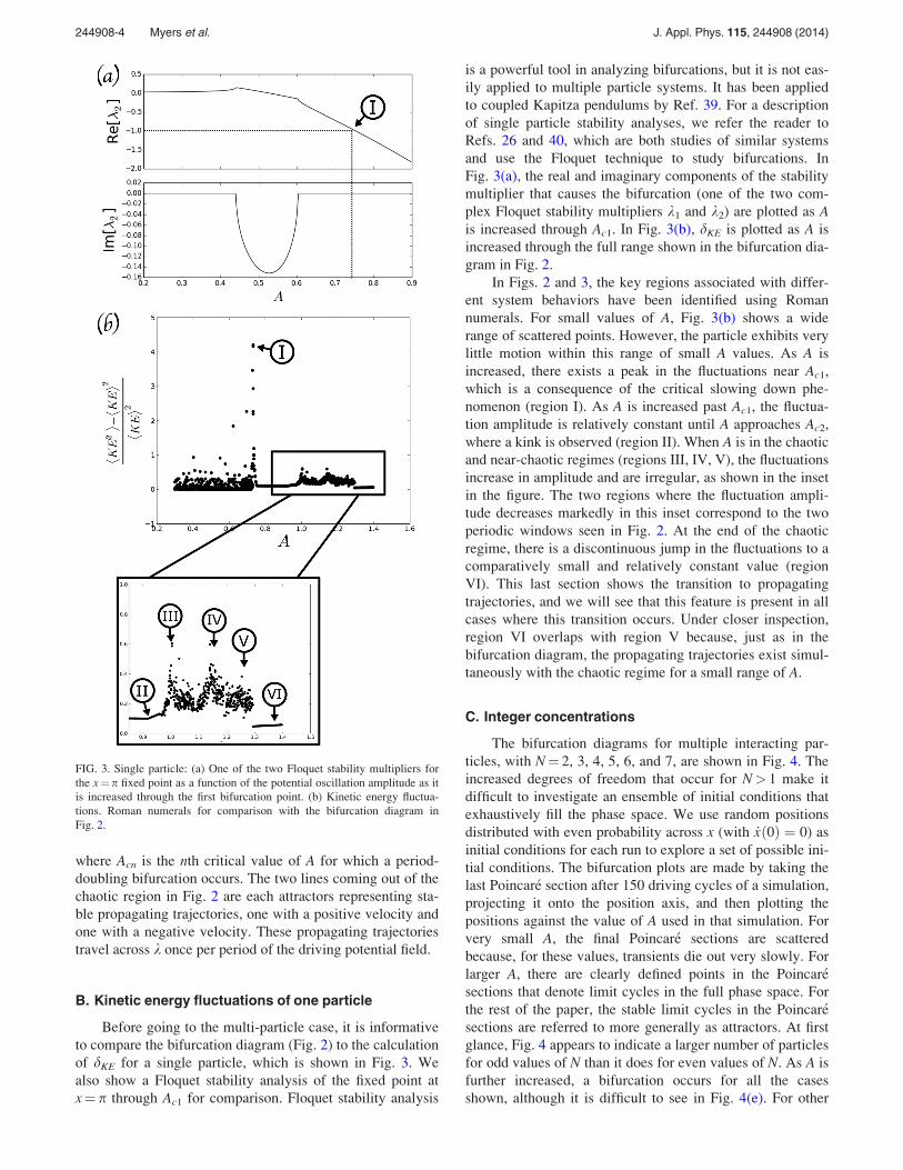
Before going to the multi-particle case, it is informativeto compare the bifurcation diagram (Fig. 2) to the calculationof dKE for a single particle, which is shown in Fig. 3. Wealso show a Floquet stability analysis of the fixed point atx¼ p through Ac1 for comparison. Floquet stability analysis

is a powerful tool in analyzing bifurcations, but it is not eas-ily applied to multiple particle systems. It has been appliedto coupled Kapitza pendulums by Ref. 39. For a descriptionof single particle stability analyses, we refer the reader toRefs. 26 and 40, which are both studies of similar systemsand use the Floquet technique to study bifurcations. InFig. 3(a), the real and imaginary components of the stabilitymultiplier that causes the bifurcation (one of the two com-plex Floquet stability multipliers k1 and k2) are plotted as Ais increased through Ac1. In Fig. 3(b), dKE is plotted as A isincreased through the full range shown in the bifurcation dia-gram in Fig. 2.

In Figs. 2 and 3, the key regions associated with differ-ent system behaviors have been identified using Romannumerals. For small values of A, Fig. 3(b) shows a widerange of scattered points. However, the particle exhibits verylittle motion within this range of small A values. As A isincreased, there exists a peak in the fluctuations near Ac1,which is a consequence of the critical slowing down phe-nomenon (region I). As A is increased past Ac1, the fluctua-tion amplitude is relatively constant until A approaches Ac2,where a kink is observed (region II). When A is in the chaoticand near-chaotic regimes (regions III, IV, V), the fluctuationsincrease in amplitude and are irregular, as shown in the insetin the figure. The two regions where the fluctuation ampli-tude decreases markedly in this inset correspond to the twoperiodic windows seen in Fig. 2. At the end of the chaoticregime, there is a discontinuous jump in the fluctuations to acomparatively small and relatively constant value (regionVI). This last section shows the transition to propagatingtrajectories, and we will see that this feature is present in allcases where this transition occurs. Under closer inspection,region VI overlaps with region V because, just as in thebifurcation diagram, the propagating trajectories exist simul-taneously with the chaotic regime for a small range of A.

C. Integer concentrations

The bifurcation diagrams for multiple interacting par-ticles, with N¼ 2, 3, 4, 5, 6, and 7, are shown in Fig. 4. Theincreased degrees of freedom that occur for N> 1 make itdifficult to investigate an ensemble of initial conditions thatexhaustively fill the phase space. We use random positionsdistributed with even probability across x (with _xð0Þ ¼ 0) asinitial conditions for each run to explore a set of possible ini-tial conditions. The bifurcation plots are made by taking thelast Poincar!e section after 150 driving cycles of a simulation,projecting it onto the position axis, and then plotting thepositions against the value of A used in that simulation. Forvery small A, the final Poincar!e sections are scatteredbecause, for these values, transients die out very slowly. Forlarger A, there are clearly defined points in the Poincar!esections that denote limit cycles in the full phase space. Forthe rest of the paper, the stable limit cycles in the Poincar!esections are referred to more generally as attractors. At firstglance, Fig. 4 appears to indicate a larger number of particlesfor odd values of N than it does for even values of N. As A isfurther increased, a bifurcation occurs for all the casesshown, although it is difficult to see in Fig. 4(e). For other

FIG. 3. Single particle: (a) One of the two Floquet stability multipliers forthe x¼p fixed point as a function of the potential oscillation amplitude as itis increased through the first bifurcation point. (b) Kinetic energy fluctua-tions. Roman numerals for comparison with the bifurcation diagram inFig. 2.

244908-4 Myers et al. J. Appl. Phys. 115, 244908 (2014)

[This article is copyrighted as indicated in the article. Reuse of AIP content is subject to the terms at: http://scitation.aip.org/termsconditions. Downloaded to ] IP:132.198.138.131 On: Mon, 22 Sep 2014 18:01:24

values of A, the diagrams in Fig. 4 appear as scattered points,implying either chaotic motion, high-period trajectories, ormotion on a torus (after a Neimark bifurcation). Past thisscattered regime, the system collapses into a new stableregime that is qualitatively similar to the propagating trajec-tories that occur after the chaotic regime in the single particlecase.

The discrepancy between the number of possible attrac-tors for odd and even values of N can be explained by con-sidering the relationship between the number of particles andthe number of antinodes in one period of the potential. Forthe trajectory (x1(t),…, x2dN(t)), the number of attractors thatare observed for values of A before the first bifurcation isequal to the number of particles when N is even and twicethe number of particles when N is odd. In other words, thereis one possible final state configuration of the whole systemwhen N is even and two possible final state configurations ofthe system when N is odd. To see why this occurs, we exam-ine in detail the cases of three and four particles per period.Figs. 5(a)–5(d) show cartoons of the final particle configura-tions for cases N¼ 4 and N¼ 3, respectively. In thesecartoons, the particle position in the periodic domain isdrawn as an angle, so that motion of the particle in the xdomain corresponds in the figure to rotation about a circle.The intersection points of the circle with a horizontal bisec-tion line occur at the antinodes of the potential U. In this fig-ure, at least one particle can always be found at the antinode

of U. From the single particle case, we know the antinodescan act as attractors, where individual particles remainmotionless in the x% _x phase plane. In the case of four par-ticles, shown in Fig. 5(a), two particles may occupy theantinodes of U and the other two particles oscillate about the

FIG. 4. Multiple particle bifurcation diagrams made by: (1) initializing particles at random initial positions with _xð0Þ ¼ 0, (2) projecting the Poincar!e sectiononto the position axis after 150 cycles and plotting against the value of A, and (3) repeating the process for 400 values of A in the range of interest. The numberof particles used in each bifurcation diagram is (a) N¼ 2, (b) N¼ 3, (c) N¼ 4, (d) N¼ 5, (e) N¼ 6, (f) N¼ 7. Note that the range of A values explored differsin each figure.

FIG. 5. The position along the periodic domain is indicated by an anglearound a circle. The black dots represent average particle positions beforethe first bifurcation. The line bisecting the circle passes through the twoantinodes of the potential field. Part (a) shows the N¼ 4 stable configurationwhich is an asymptotically stable fixed point in the Poincar!e sections of thefull phase space. Part (b) is an N¼ 4 unstable configuration which is theunstable fixed point in the Poincar!e sections of the full phase space. Parts (c)and (d) show two different possible stable configurations for N¼ 3, both ofwhich are stable fixed points in the Poincar!e sections of the full phase space.

244908-5 Myers et al. J. Appl. Phys. 115, 244908 (2014)

[This article is copyrighted as indicated in the article. Reuse of AIP content is subject to the terms at: http://scitation.aip.org/termsconditions. Downloaded to ] IP:132.198.138.131 On: Mon, 22 Sep 2014 18:01:24

nodes of U. One might imagine that a rotation of this config-uration by p/4 (shown in Fig. 5(b)) might be a fixed point inthe Poincar!e section of the full phase space, and indeed it is,but it is not a stable configuration and, unless perfectly con-figured, it will collapse into the configuration shown inFig. 5(a). For three particles, one particle sits at antinode andthe two remaining particles compete over the other antinode,as shown in Figs. 5(c) and 5(d). Which antinode a particle isattracted to depends on the initial conditions. In both the fourand three particle cases, the particles at the antinodes arestationary.

Drawing lines between the adjacent average particlepositions in the circular topology creates a regular convexpolygon inscribing the circle. From our description of theparticle behavior above, at least one vertex of the polygonmust be at an antinode. For a regular polygon inscribing thecircle with an even number of vertices, each antinode maytouch a vertex and it is symmetric under all rotations obeyingthis rule. For a polygon with an odd number of vertices, how-ever, only one vertex can occupy an antinode so that rota-tions by p/N flip the symmetry about a line verticallybisecting the circle. There are always two unique possiblestable configurations when N is odd, but only one when N iseven. This picture changes for even values of N when N> 6.For N> 6, the stable configuration no longer occurs for apair of particles located at each antinode, but rather for pairsoscillating on either side of the antinodes much like what isshown in Fig. 5(b) but with an extra particle on the top andbottom of the circle.

In Fig. 6, the value of A at which the first bifurcationoccurs is plotted as a function of N, with separate lines for Neven (red squares) and N odd (blue triangles). A strikingcharacteristic of Fig. 6 is that between N¼ 6 and N¼ 8, thereis a cross-over point at which the even N line jumps upward

and crosses through the odd N line. This sudden jump in theeven N line between N¼ 6 and N¼ 8 occurs due to a changein type of first bifurcation. The first bifurcation when N¼ 6as well as the first bifurcations for all lower even values of Nare Neimark bifurcations (a.k.a bifurcation to a torus) inwhich N stability multipliers cross the unit circle with non-zero imaginary components. Half of those stability multi-pliers (N/2) that cross the unit circle have positive imaginarycomponents and the other half have the complementarynegative imaginary components. For N¼ 8 and all highereven values of N, the first bifurcation becomes a cyclic foldbifurcation, although the bifurcations for odd values of Nremain supercritical flip bifurcations.

We can qualitatively understand the transition whichoccurs when N is changed from six to eight in Fig. 6 byobserving how the bifurcation diagrams, and therefore thestable attractors, depend on the particle number. In Fig. 4(e),after the first bifurcation, the particle motions are quenchedby the presence of other attractors. For the sake of discus-sion, we distinguish the two competing sets of attractorsbased on whether they are found at the far left or far rightedges of the diagrams, respectively. Comparing the cases ofN¼ 2, N¼ 4, and N¼ 6 in Fig. 4, we see similar rightmostattractors that appear abruptly at different values of A ineach case. As N (even) increases, the rightmost attractorsincreasingly impinge on the leftmost attractors. Thisimpingement is responsible for the crossing of the lines inFig. 6. When N increases from six to eight, the rightmostattractors extinguish the left most attractors and become thefirst available attractors for N( 8 (even). These new firstattractors, previously the rightmost, represent a fundamen-tally different type of limit cycle in the full phase space thanwhat was previously first available. Therefore, when thisattractor first bifurcates, it falls outside of the original pro-gression, causing the jump in Ac1 as N is changed from six toeight shown in Fig. 6.

For all of the cases shown in Fig. 4, the system eventu-ally collapses back into clearly defined attractors which havethe form of “propagating” trajectories, as was also observedfor the single particle case. These attractors display non-zeronet particle motion of one particle when N is odd, but no netmotion when N is even. The particles travel in either the 6xdirection before a collision-like event. After the “collision,”they travel in the opposite direction having exchanged somekinetic energy with the particle with which the collisionoccurred. When N is odd the transport of one particle occurseither in the 6x direction depending on the initial conditions.There is no possible counter-propagating particle pair forone of the particles with N odd.

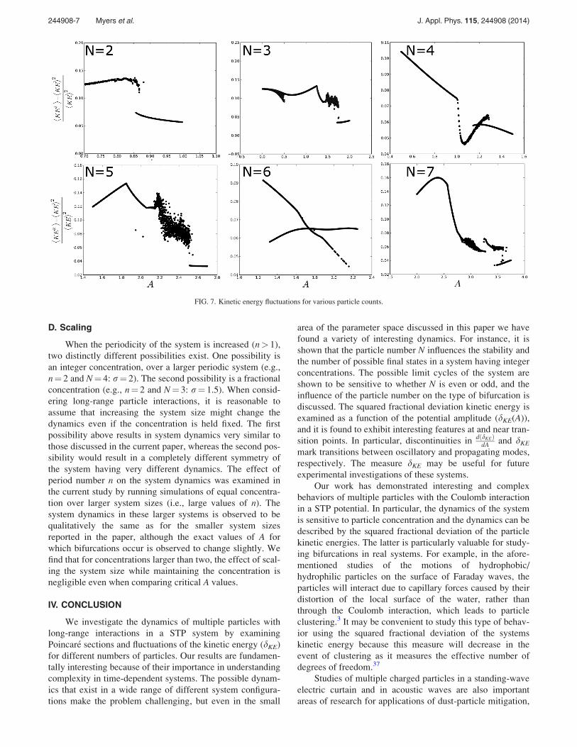
In Fig. 7, the squared fractional deviation of the kineticenergy dKE is plotted for all of the bifurcation diagramsshown in Fig. 4. These plots all exhibit a discontinuity at thepoint corresponding to transition to a state with the propagat-ing trajectories. The discontinuity is not as clear in Fig. 7(e)because (as can be observed in the corresponding bifurcationdiagram Fig. 4(e)) the propagating trajectory begins beforethe first bifurcation. In Fig. 7(e), the curve starting belowand crossing at A ) 1.75 indicates the values of dKE for thepropagating trajectory.

FIG. 6. A plot of the value of A at which the system first bifurcates (Ac1) asa function of the number of particles in simulation (N). Even particle num-bers are shown with red squares and odd particle numbers are shown withblue triangles. A cross-over between the N odd and N even curves occursbetween N¼ 6 and N¼ 7, which corresponds to the first bifurcation for theeven value of N changing from a Neimark bifurcation to a cyclic fold bifur-cation. The N odd bifurcations are all supercritical flip bifurcations for thevalues of N shown here. The upper (lower) error bound is the value of Awhich we are certain is after (before) the bifurcation. The error bounds areseen to be quite small in the figure.

244908-6 Myers et al. J. Appl. Phys. 115, 244908 (2014)

[This article is copyrighted as indicated in the article. Reuse of AIP content is subject to the terms at: http://scitation.aip.org/termsconditions. Downloaded to ] IP:132.198.138.131 On: Mon, 22 Sep 2014 18:01:24

D. Scaling

When the periodicity of the system is increased (n> 1),two distinctly different possibilities exist. One possibility isan integer concentration, over a larger periodic system (e.g.,n¼ 2 and N¼ 4: r¼ 2). The second possibility is a fractionalconcentration (e.g., n¼ 2 and N¼ 3: r¼ 1.5). When consid-ering long-range particle interactions, it is reasonable toassume that increasing the system size might change thedynamics even if the concentration is held fixed. The firstpossibility above results in system dynamics very similar tothose discussed in the current paper, whereas the second pos-sibility would result in a completely different symmetry ofthe system having very different dynamics. The effect ofperiod number n on the system dynamics was examined inthe current study by running simulations of equal concentra-tion over larger system sizes (i.e., large values of n). Thesystem dynamics in these larger systems is observed to bequalitatively the same as for the smaller system sizesreported in the paper, although the exact values of A forwhich bifurcations occur is observed to change slightly. Wefind that for concentrations larger than two, the effect of scal-ing the system size while maintaining the concentration isnegligible even when comparing critical A values.

IV. CONCLUSION

We investigate the dynamics of multiple particles withlong-range interactions in a STP system by examiningPoincar!e sections and fluctuations of the kinetic energy (dKE)for different numbers of particles. Our results are fundamen-tally interesting because of their importance in understandingcomplexity in time-dependent systems. The possible dynam-ics that exist in a wide range of different system configura-tions make the problem challenging, but even in the small

area of the parameter space discussed in this paper we havefound a variety of interesting dynamics. For instance, it isshown that the particle number N influences the stability andthe number of possible final states in a system having integerconcentrations. The possible limit cycles of the system areshown to be sensitive to whether N is even or odd, and theinfluence of the particle number on the type of bifurcation isdiscussed. The squared fractional deviation kinetic energy isexamined as a function of the potential amplitude (dKE(A)),and it is found to exhibit interesting features at and near tran-sition points. In particular, discontinuities in dðdKEÞ

dA and dKE

mark transitions between oscillatory and propagating modes,respectively. The measure dKE may be useful for futureexperimental investigations of these systems.

Our work has demonstrated interesting and complexbehaviors of multiple particles with the Coulomb interactionin a STP potential. In particular, the dynamics of the systemis sensitive to particle concentration and the dynamics can bedescribed by the squared fractional deviation of the particlekinetic energies. The latter is particularly valuable for study-ing bifurcations in real systems. For example, in the afore-mentioned studies of the motions of hydrophobic/hydrophilic particles on the surface of Faraday waves, theparticles will interact due to capillary forces caused by theirdistortion of the local surface of the water, rather thanthrough the Coulomb interaction, which leads to particleclustering.3 It may be convenient to study this type of behav-ior using the squared fractional deviation of the systemskinetic energy because this measure will decrease in theevent of clustering as it measures the effective number ofdegrees of freedom.37

Studies of multiple charged particles in a standing-waveelectric curtain and in acoustic waves are also importantareas of research for applications of dust-particle mitigation,

FIG. 7. Kinetic energy fluctuations for various particle counts.

244908-7 Myers et al. J. Appl. Phys. 115, 244908 (2014)

[This article is copyrighted as indicated in the article. Reuse of AIP content is subject to the terms at: http://scitation.aip.org/termsconditions. Downloaded to ] IP:132.198.138.131 On: Mon, 22 Sep 2014 18:01:24

e.g., from a solar panel.31 Charged particles interacting instanding-wave electric curtains and standing-wave acousticfields exhibit complicated dynamics that may be illuminatedby studying the squared fractional deviation of the particlekinetic energy. For example, in Ref. 41, it was observed thatfor charged particles in a standing-wave acoustic field, rela-tive motion of smaller particles is faster than that of largerparticles, so that the large particles act as collectors withinsome agglomeration volume. Any small particles present inthe agglomeration volume are likely to aggregate to a largerparticle, and this aggregation is desirable for applicationssuch as cleaning particles from surfaces. A sweep of theacoustic driving parameters to find the configuration forwhich maximal aggregations occurs could clearly be foundand described in terms of the minimal squared fractionaldeviation of the particle kinetic energies, again due to itsmeasure of the effective number of degrees of freedom. Ingeneral, we hope our work may stimulate further research ofSTP systems with interacting particles and shed some lighton their complicated and exciting dynamics.

ACKNOWLEDGMENTS

This work was supported by NASA Space GrantConsortium under Grant Nos. NNX10AK67H, NNX08AZ07A,and NNX13AD40A. We also want to acknowledge theVermont Advanced Computing Core which was supported byNASA (NNX 06AC88G), at the University of Vermont forproviding the high performance computing resources used forthe work in this paper.

1T. Simpson, J. Liu, and A. Gavrielides, “Period-doubling cascades andchaos in a semiconductor laser with optical injection,” Phys. Rev. A 51,4181–4185 (1995).

2P. Olbrich, J. Karch, E. L. Ivchenko, J. Kamann, B. M€arz, M.Fehrenbacher, D. Weiss, and S. D. Ganichev, “Classical ratchet effects inheterostructures with a lateral periodic potential,” Phys. Rev. B 83,165320 (2011).

3N. Francois, H. Xia, H. Punzmann, and M. Shats, “Inverse energy cascadeand emergence of large coherent vortices in turbulence driven by faradaywaves,” Phys. Rev. Lett. 110, 194501 (2013).

4P. Denissenko, G. Falkovich, and S. Lukaschuk, “How waves affect thedistribution of particles that float on a liquid surface,” Phys. Rev. Lett. 97,244501 (2006).

5G. Falkovich, A. Weinberg, P. Denissenko, and S. Lukaschuk, “Floaterclustering in a standing wave,” Nature 435, 1045 (2005).

6E. Boukobza, M. G. Moore, D. Cohen, and A. Vardi, “Nonlinear phasedynamics in a driven bosonic josephson junction,” Phys. Rev. Lett. 104,240402 (2010).

7P. Bak, C. Tang, and K. Wisenfeld, “Self-organized criticality: An expla-nation of 1/f noise,” Phys. Rev. Lett. 59, 381 (1987).

8P. Bak, K. Chen, and M. Creutz, “Self-organized criticality in the game oflife,” Nature 342, 780 (1989).

9E. A. Martens, S. Thutupalli, A. Fourriere, and O. Hallatchek, “Chimerastates in mechanical oscillator networks,” Proc. Natl. Acad. Sci. U. S. A.110, 10563–10567 (2013).

10M. I. Rabinovich, P. Varona, A. I. Selverston, and H. D. I. Abarbanel,“Dynamical principles in neuroscience,” Rev. Mod. Phys. 78, 1213–1265(2006).

11A. J. Rimberg, T. R. Ho, I. M. C. Kurdak, J. Clarke, K. L. Campman, andA. C. Gossard, “Dissipation-driven superconductor-insulator transition in

a two-dimensional josephson-junction array,” Phys. Rev. Lett. 78,2632–2635 (1997).

12P. L. Kapitza, “Dynamical stability of a pendulum when its point ofsuspension vibrates,” Zh. Eksp. Teor. Fiz. 21, 588 (1951).

13P. L. Kapitza, “Pendulum with a vibrating suspension,” Usp. Fiz. Nauk 44,7–20 (1951); available at http://ufn.ru/ru/articles/1951/5/c/.

14S. Lefschetx, Differential Equations Geometric Theory, 2nd ed. (DoverPublications, New York, 1977).

15N. W. McLachlan, Theory and Application of Mathieu Functions, 1st ed.(Oxford University Press, London, 1947).

16T. Pradhan and A. V. Khare, “Plane pendulum in quantum mechanics,”Am. J. Phys. 41, 59–66 (1973).

17D. Leibfried, R. Blatt, C. Monroe, and D. Wineland, “Quantum dynamicsof single trapped ions,” Rev. Mod. Phys. 75, 281–324 (2003).

18L. Ruby, “Applications of the Mathieu equation,” Am. J. Phys. 64, 39–44(1996).

19N. N. Bogoljubov and Y. A. Mitropolski, Asymptotic Methods in theTheory of Nonlinear Oscillations (Gordon and Breach, New York, 1961).

20L. D!alessio and A. Polkovnikov, “Many-body energy localization transi-tion in periodically driven systems,” Ann. Phys. 333, 19–33 (2013).

21J. Starrett and R. Tagg, “Control of a chaotic parametrically driven pendu-lum,” Phys. Rev. Lett. 74, 1974–1977 (1994).

22R. Chacon and L. Marcheggiani, “Controlling spatiotemporal chaos inchains of dissipative kapitza pendula,” Phys. Rev. E 82, 016201 (2010).

23D. Maravall, C. Zhou, and J. Alonso, “Hybrid fuzzy control of the invertedpendulum via vertical forces,” Int. J. Intell. Syst. 20, 195–211 (2005).

24J. A. Blackburn, “Stability and hopf bifurcations in an inverted pendulum,”Am. J. Phys. 60, 903 (1992).

25W. Szemplinska-Stupnicka, E. Tyrkiel, and A. Zubrzycki, “The globalbifurcations that lead to transient tumbling chaos in a parametricallydriven pendulum,” Int. J. Bifurcation Chaos 10(9), 2161–2175 (2000).

26S. Kim and B. Hu, “Bifurcations and transitions to chaos in an invertedpendulum,” Phys. Rev. E 58, 3028–3035 (1998).

27M. V. Bartuccelli, G. Gentile, and K. V. Georgiou, “On the dynamics of avertically driven damped planar pendulum,” R. Soc. 457, 3007–3022 (2001).

28E. Butikov, “Subharmonic resonances of the parametrically driven pendu-lum,” J. Phys. A: Math. Gen. 35, 6209 (2002).

29R. W. Leven and B. P. Koch, “Chaotic behaviour of a parametricallyexcited damped pendulum,” Phys. Lett. 86A, 71 (1981).

30S. Masuda, K. Fujibayashi, K. Ishida, and H. Inaba, “Confinement andtransportation of charged aerosol clouds via electric curtain,” Electr. Eng.Jpn. 92, 43 (1972).

31G. Liu and J. Marshall, “Particle transport by standing waves on an electriccurtain,” J. Electrost. 68, 289–298 (2010).

32J. Chesnutt and J. S. Marshall, “Simulation of particle separation on aninclined electric curtain,” IEEE Trans. Ind. Appl. 49, 1104–1112 (2013).

33J. S. Marshall, “Particle clustering in periodically forced straining flows,”J. Fluid Mech. 624, 69 (2009).

34P. Gibbon and G. Sutmann, “Long-range interactions in many-particlesimulation,” Quantum Simulations of Complex Many-Body Systems: FromTheory to Algorithms, edited by J. Grotendorst, D. Marx and A.Muramatsu, (John von Neumann Institute for Computing, J€ulich, 2002),NIC Series Vol. 10, pp. 467–506.

35J. Guckenheimer, Nonlinear Oscillations, Dynamical Systems, andBifurcations of Vector Fields (Springer-Verlag, New York, 1983).

36M. Scheffer, J. Bascompte, W. A. Brock, V. Brovkin, S. R. Carpenter, V.Dakos, H. Held, E. H. V. Nes, M. Rietkerk, and G. Sugihara, “Early-warn-ing signals for critical transitions,” Nature 461, 53–59 (2009).

37F. Cecconi, F. Diotallevi, U. M. B. Marconi, and A. Puglisi, “Fluid-like behav-ior of a one-dimensional granular gas,” J. Chem. Phys. 120, 35–42 (2004).

38J. Thompson and H. Stewart, Nonlinear Dynamics and Chaos, 2nd ed.(Wiley, New York, 2002).

39S.-Y. Kim and B. Hu, “Critical behavior of period doublings in coupledinverted pendulums,” Phys. Rev. E 58, 7231–7242 (1998).

40O. D. Myers, J. Wu, and J. S. Marshall, “Nonlinear dynamics of particlesexcited by an electric curtain,” J. Appl. Phys. 114, 154907 (2013).

41D. Chen and J. Wu, “Dislodgement and removal of dust-particles from asurface by a technique combining acoustic standing wave and airflow,”J. Acoust. Soc. Am. 127, 45–50 (2010).

244908-8 Myers et al. J. Appl. Phys. 115, 244908 (2014)

[This article is copyrighted as indicated in the article. Reuse of AIP content is subject to the terms at: http://scitation.aip.org/termsconditions. Downloaded to ] IP:132.198.138.131 On: Mon, 22 Sep 2014 18:01:24