computational structural analysis
TRANSCRIPT

Politecnico di Milano
Department of Civil and Environmental Engineering
Computational Structural Analysis
Modeling and Implementation for Frame Structures
Report
Presented by
Diyan Rashevski, 816971
Supervisors:
Prof. Fabio Biondini
Dr. Andrea Titi
July 2014


III
ABSTRACT
The aim of this report is to present the result of algorithm development for machine support-
ed structural analysis. The theoretical foundations are considered with an accent on the
computational clarity, efficiency and accuracy. Based on this knowledge practical calculation
mechanisms are formulated and utilized to achieve the final product that is entirely opera-
tional and validated software for solving plane static structural problems. The motivation be-
hind is not the lack of similar programs but gaining a comprehensive insight into their con-
struction, algorithms and techniques in order to remain fully aware of potential problems and
risks as users of computer codes, especially closed commercial ones.

IV
TABLE OF CONTENTS
List of Figures ..................................................................................................................... VIII
List of Tables ......................................................................................................................... X
Nomenclature ....................................................................................................................... XI
1 Introduction ................................................................................................................... 1
2 Theoretical Background ................................................................................................ 2
2.1 Principle of Virtual Work .......................................................................................... 2
2.1.1 Principle of Virtual Displacements ..................................................................... 2
2.1.2 Principle of Virtual Forces ................................................................................. 3
2.2 Displacement Method .............................................................................................. 3
2.2.1 Basic Concept ................................................................................................... 3
2.2.2 Procedure and Governing Equations ................................................................ 4
2.3 Matrix Analysis ........................................................................................................ 5
2.3.1 Direct Stiffness Method ..................................................................................... 5
2.3.2 Features of the Stiffness Matrix ......................................................................... 7
2.3.3 Linear Elasticity in Matrix Form ......................................................................... 8
3 Description of Structural System ................................................................................... 9
3.1 Geometry ................................................................................................................. 9
3.2 Topology .................................................................................................................. 9
3.2.1 Kinematic Boundary Conditions ........................................................................ 9
3.2.2 Static Boundary Conditions ............................................................................. 10
3.2.3 Internal Constraints ......................................................................................... 10
3.2.4 Elements and Incidences ................................................................................ 10
3.3 Cross-Sections ...................................................................................................... 10
3.4 Materials ................................................................................................................ 11
4 Numbering of The Degrees of Freedom ...................................................................... 12
4.1 Initialization ............................................................................................................ 12
4.2 Restraints and Links .............................................................................................. 12
4.3 Discretization ......................................................................................................... 12
5 Nodal Loads in The Global Reference System ............................................................ 14
5.1 Input and Initialization ............................................................................................ 14
5.2 Global Arrangement ............................................................................................... 14
6 Element Properties in The Local Reference System .................................................... 15
6.1 Equivalent Nodal Force Vector .............................................................................. 15

V
6.1.1 Sign Convention and Procedure ..................................................................... 15
6.1.2 Self-Weight ..................................................................................................... 17
6.2 Stiffness Matrix ...................................................................................................... 18
7 Transformation of The Reference System ................................................................... 19
7.1 Problem Statement ................................................................................................ 19
7.2 Transformation of 2D Coordinate System .............................................................. 19
7.2.1 2D Beam Element Transformation Matrix ........................................................ 20
7.2.2 Features and Application of the Transformation Matrix ................................... 20
8 Structural Assembly .................................................................................................... 22
8.1 Assembly Matrix .................................................................................................... 22
8.2 Direct Assembly ..................................................................................................... 22
9 Solution of The Linear System .................................................................................... 24
9.1 Gauss Elimination Method ..................................................................................... 24
9.2 Conditioning of the Linear Equation System .......................................................... 25
9.2.1 Evaluation of Condition Number (a-priori) ....................................................... 26
9.2.2 Diagonal Decay Error Test (in-progress) ......................................................... 27
9.2.3 Work of Residuals (posteriori) ......................................................................... 27
10 Stress Analysis ............................................................................................................ 28
10.1 Sign Convention .................................................................................................... 28
10.2 Internal Reactions .................................................................................................. 28
11 Specialized Problems .................................................................................................. 30
11.1 Prestressing........................................................................................................... 30
11.1.1 Basic Principle and Technology ...................................................................... 30
11.1.2 Prestressing Losses ........................................................................................ 31
11.1.3 Implementation ............................................................................................... 33
11.2 Elastic Constraints and Links ................................................................................. 34
11.3 Imposed Displacements ........................................................................................ 35
11.3.1 Absolute Displacements .................................................................................. 35
11.3.2 Relative Displacements ................................................................................... 35
11.3.3 Inclined Constraints ........................................................................................ 36
11.4 Elastic Foundation ................................................................................................. 36
12 Benchmarks ................................................................................................................ 38
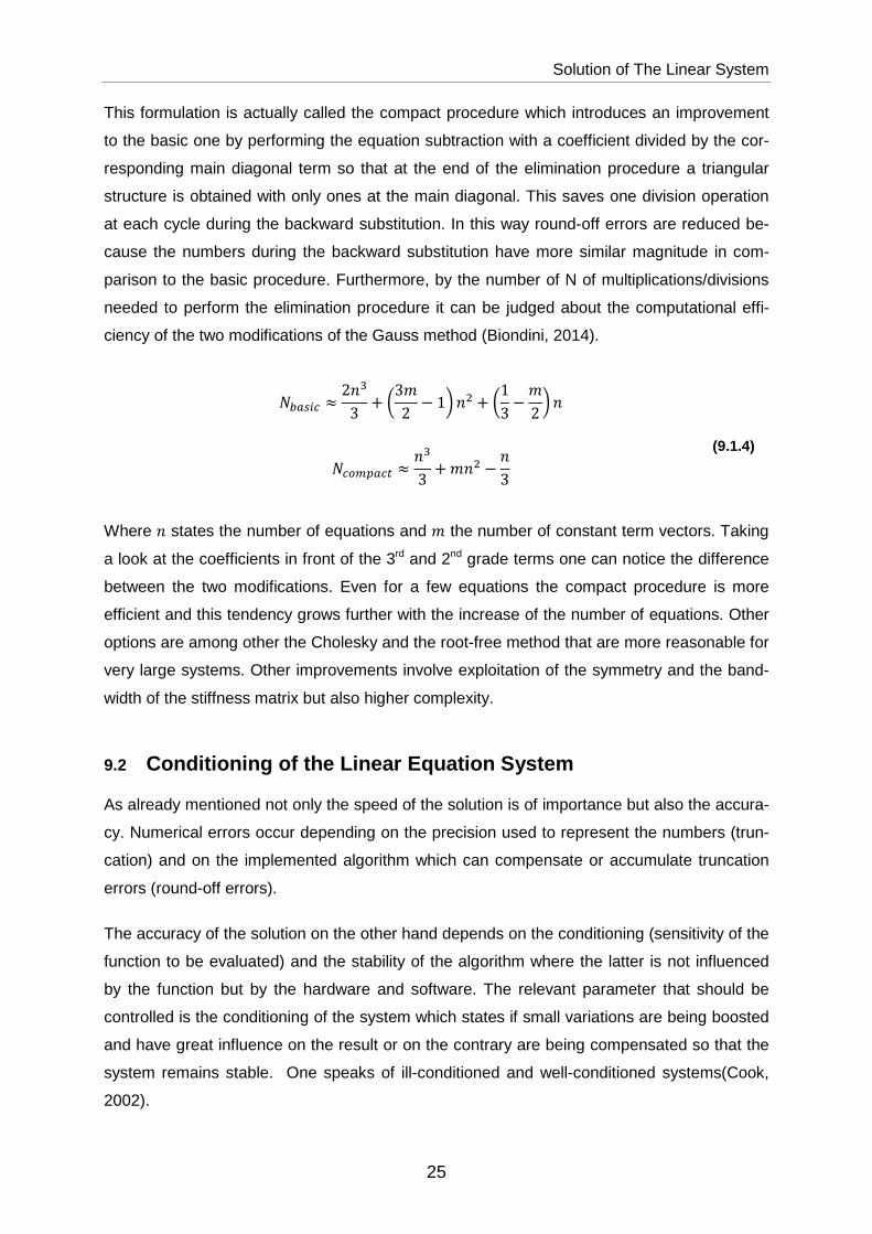
12.1 Clamped Beam with Nodal Load: Influence of Shear Deformability ....................... 38
12.2 Frame with Uniform Temperature Change ............................................................. 40
12.3 Frame with Pinned Joints and Foundation Settlement ........................................... 43
12.4 Frame with Elastic Restraints and Linear Differential Temperature Change .......... 47

VI
12.5 Portal Frame with Inclined Roof Beams and Tie Rod ............................................. 50
12.6 Two Frame Systems Subjected To Various Loads ................................................ 53
12.7 Single Beams ........................................................................................................ 55
12.8 Prestressing........................................................................................................... 61
12.9 Beam on Elastic Foundation .................................................................................. 63
13 Application: Railway Bridge with Gerber Joints ............................................................ 64
14 Summary ..................................................................................................................... 75
15 References .................................................................................................................. 76
Appendix A: Flowchart of The Code ..................................................................................... 77
Appendix B: User Manual ..................................................................................................... 79
Appendix C: Fortran Listing .................................................................................................. 87

VII
List of Figures
VIII
LIST OF FIGURES
Figure 2.1: Statically undetermined system with multiple possible basic systems ......................................................................................................... 4
Figure 2.2: Plane beam element in global reference system ............................. 6
Figure 2.3: Plane beam element in global reference system ............................. 6
Figure 2.4: Typical symmetrical sparse matrix with constant bandwidth = 3 ...... 7
Figure 3.1: Plane frame system (left) and its discretization with DOFs (right) .. 13
Figure 6.1: Element loading with equivalent nodal forces. Sign convention ..... 15
Figure 6.2: Beam with both ends fixed ............................................................. 16
Figure 6.3: Fix end moments according to load case ....................................... 16
Figure 7.1: Beam element in local (left) and global (right) reference system ... 19
Figure 7.2: Sin and cos relations...................................................................... 20
Figure 8.1: Example for global stiffness matrix with assembling steps ............ 23
Figure 10.1: Sign convention for element nodal forces (left) and internal reactions (right) ............................................................................................. 28
Figure 11.1: Stresses resulting from prestressing, constant and variable external loading ........................................................................................... 30
Figure 11.2: Production procedure with pre-tensioning in prestressing bed ...... 31
Figure 11.3: Tendon redirection (with post-tensioning) ...................................... 31
Figure 11.4: Equilibrium for friction losses according to Coulomb - Couley ....... 32
Figure 11.5: Prestressing element in local reference system ............................. 33
Figure 11.6: Elastic restraint (left) and link (right) .............................................. 34
Figure 11.7: Beam element on elastic foundation .............................................. 36
Figure 12.1: Clamped beam with nodal load ...................................................... 38
Figure 12.2: Deformed shape: Clamped beam with nodal load ......................... 39
Figure 12.3: Shear force diagram: Clamped beam with nodal load ................... 39
Figure 12.4: Bending moment diagram: Clamped beam with nodal load ........... 40
Figure 12.5: Frame with uniform ∆T ................................................................... 40
Figure 12.6: Deformed shape: Frame with uniform ∆T ...................................... 41
Figure 12.7: Axial force: Frame with uniform ∆T ................................................ 41
Figure 12.8: Shear force: Frame with uniform ∆T .............................................. 42
Figure 12.9: Bending moment: Frame with uniform ∆T ...................................... 43
Figure 12.10: Frame with Pinned Joints and Foundation Settlement ................... 43
Figure 12.11: Deformed shape: Frame with Pinned Joints and Foundation Settlement ...................................................................................... 44
Figure 12.12: Axial force: Frame with Pinned Joints and Foundation Settlement 45
Figure 12.13: Shear force: Frame with Pinned Joints and Foundation Settlement .. ....................................................................................................... 46
Figure 12.14: Bending moment: Frame with Pinned Joints and Foundation Settlement ...................................................................................... 46
Figure 12.15: Frame with elastic restraints and linear ∆T .................................... 47
Figure 12.16: Deformed shape: Frame with elastic restraints and linear ∆T ........ 48
Figure 12.17: Axial force: Frame with elastic restraints and linear ∆T.................. 48
Figure 12.18: Shear force: Frame with elastic restraints and linear ∆T ................ 49
Figure 12.19: Bending moment: Frame with elastic restraints and linear ∆T ....... 50
Figure 12.20: Frame with inclined roof beams and tie rod ................................... 50
Figure 12.21: Deformed shape: Frame with inclined roof beams and tie rod ....... 51
Figure 12.22: Axial force: Frame with inclined roof beams and tie rod................. 51

List of Figures
IX
Figure 12.23: Shear force: Frame with inclined roof beams and tie rod ............... 52
Figure 12.24: Bending moment: Frame with inclined roof beams and tie rod ...... 53
Figure 12.25: The two frame systems without loading ......................................... 53
Figure 12.26: Simple beam – uniformly distributed load ...................................... 56
Figure 12.27: Simple beam – uniform load partially distributed ........................... 56
Figure 12.28: Simple beam – uniform load partially distributed at one end.......... 57
Figure 12.29: Simple beam – uniform load partially distributed at each end ........ 57
Figure 12.30: Simple beam – load increasing uniformly to one end .................... 58
Figure 12.31: Simple beam – load increasing uniformly to center ....................... 58
Figure 12.32: Simple beam – concentrated load at center ................................... 59
Figure 12.33: Simple beam – concentrated load at any point .............................. 59
Figure 12.34: Simple beam – two equal concentrated loads symmetrically placed . ....................................................................................................... 59
Figure 12.35: Simple beam – two equal concentrated loads unsymmetrically placed ............................................................................................ 60
Figure 12.36: Simple beam – two unequal concentrated loads unsymmetrically placed ............................................................................................ 60
Figure 12.37: Beam on elastic foundation subjected to linear load ...................... 63
Figure 13.1: Railway bridge with gerber joints ................................................... 64
Figure 13.2: Structural model without discretization........................................... 64
Figure 13.3: Discretization for load case 1 ......................................................... 66
Figure 13.4: Structural response to load case 1 ................................................ 66
Figure 13.5: Discretization for load case 2 ......................................................... 67
Figure 13.6: Structural response to load case 2 ................................................ 67
Figure 13.7: Discretization for load case 3 ......................................................... 68
Figure 13.8: Structural response to load case 3 ................................................ 68
Figure 13.9: Result comparison: Load case 1 without calibration ...................... 70
Figure 13.10: Result comparison: Load case 1 with calibration ........................... 70
Figure 13.11: Result error comparison: Load case 1 ........................................... 71
Figure 13.12: Result comparison: Load case 2 without calibration ...................... 71
Figure 13.13: Result comparison: Load case 2 with calibration ........................... 72
Figure 13.14: Result error comparison: Load case 2 ........................................... 72
Figure 13.15: Result comparison: Load case 3 without calibration ...................... 73
Figure 13.16: Result comparison: Load case 3 with calibration ........................... 73
Figure 13.17: Result error comparison: Load case 3 ........................................... 74

List of Tables
X
LIST OF TABLES
Table 12.1: Results comparison: LC1, System 1 .............................................. 54
Table 12.2: Results comparison: LC2, System 1 .............................................. 54
Table 12.3: Results comparison: LC3, System 1 .............................................. 54
Table 12.4: Results comparison: LC1, System 2 .............................................. 54
Table 12.5: Results comparison: LC2, System 2 .............................................. 54
Table 12.6: Results comparison: LC3, System 2 .............................................. 55
Table 12.7: Variables relative to the I/O ............................................................ 56
Table 12.8: Results comparison: Simple beam – uniformly distributed load ..... 56
Table 12.9: Results comparison: Simple beam – uniform load partially distributed ...................................................................................... 56
Table 12.10: Results comparison: Simple beam – uniform load partially distributed at one end .................................................................... 57
Table 12.11: Results comparison: Simple beam – uniform load partially distributed at each end................................................................... 58
Table 12.12: Results comparison: Simple beam – load increasing uniformly to one end .......................................................................................... 58
Table 12.13: Results comparison: Simple beam – load increasing uniformly to center ............................................................................................. 58
Table 12.14: Results comparison: Simple beam – concentrated load at center . 59
Table 12.15: Results Comparison: Simple beam – concentrated load at any point ....................................................................................................... 59
Table 12.16: Results comparison: Simple beam – two equal concentrated loads symmetrically placed...................................................................... 60
Table 12.17: Results comparison: Simple beam – two equal concentrated loads unsymmetrically placed.................................................................. 60
Table 12.18: Results comparison: Simple beam – two unequal concentrated loads unsymmetrically placed ........................................................ 61
Table 12.19: Analytical results for different tendon layouts (P = 1) ..................... 62
Table 12.20: Numerical results for different tendon layouts (P = 1) .................... 63
Table 13.1: Element characteristics of the bridge key segments ...................... 65
Table 13.2: Experimental data .......................................................................... 69

Nomenclature
XI
NOMENCLATURE
Sign Designation Unit
� Modulus of Elasticity ����
� Moment of Inertia ��� � Span Length ��
� Cross-Section Area ��² Poisson’s ratio [−] � Coefficient of Thermal Expansion ��� � Shear Correction Factor [−] � Shear Modulus
���� ℎ Section Depth ��
� Specific Weight ���³
� Density �����

Introduction
1
1 INTRODUCTION
Computer programs are nowadays an essential part of the designing process of all kinds of
constructions. Their impact has been increasing for the last decades proportionally with the
development of hardware and other supporting calculation software and algorithms that ena-
ble more and more people to get involved in the development of a program. Practically each
university department has its own product that is being constantly improved and applied not
only for academic but also for practical purposes on private companies’ demand. The in-
creasing popularity of software is not only driven from simplicity and time saving but also
from the possibilities that it offers in terms of complexity.
At this level of computer aided calculations one might struggle upon some particular difficul-
ties including incomplete theoretical coverage of the conducted calculations or lack of trans-
parency regarding the algorithms implemented in commercial codes. In practical sense this
means increasing the risk.
Safety and efficiency is the main goal of the engineer. This is accomplishable with the help of
computational software. However, in order to further minimize the risk and maximize the effi-
ciency an entire algorithm is developed starting from scratch guided by the thought that it is
the best possible way to understand in profundity the matter and to gain useful skills when
applying the acquired knowledge.
The current report leads the reader from the theoretical foundations through the most basic
structure of a program to enhanced features, validation and application of the final software
product.

Theoretical Background
2
2 THEORETICAL BACKGROUND
Before starting with the practical implementation of a computer code first the theoretical ba-
ses should be clearly defined, discussed and synthesized so to be utilized on a later stage.
2.1 Principle of Virtual Work
One fundamental principle when analyzing structural problems is the principle of virtual work.
The name derives from the fact that work equations are formulated on fictitious (virtual) sys-
tem and related to the actual one subjected to fictitious loading case. In general the concept
can be separated in two main parts: principle of virtual displacements and principle of virtual
forces (Corigliano, 2005; Ghali, 2003).
2.1.1 Principle of Virtual Displacements
In this case the external virtual work is formulated as the product of the actual external forces
and the virtual displacements (2.2.3) which has to be equal to the internal virtual work (or
virtual strain energy) (2.2.4) expressed by the product of the actual internal forces and the
virtual internal set of displacements (2.2.2). This virtual set of displacements must be com-
patible with the boundary conditions and the virtual strain with the kinematic relation (2.2.1).
At this stage it is useful to introduce also the hypothesis of small displacements so that in the
kinematic equation for the strain-displacement relation the higher order terms are neglected.
This relation is utilized also for the virtual strain. Formulated for a continuum body with ho-
mogenous Dirichlet boundaries SU and Neumann boundary SF and subjected to surface and
body forces the equations can be listed in this form where � states the fictitious origin of the
variable (Corigliano, 2005):
���� = 12 (�$�,� + �$�,�) (2.1.1)
�(�)* = + ,������-./ (2.1.2)
�(01* = + 2��$�-./ ++ 3��$�-456 (2.1.3)
�(�)* − �(01* = 0 (2.1.4)

Theoretical Background
3
Fulfilling these equations and the compatibility conditions combined with linear elastic behav-
ior of the system ensures equilibrium and stability of the solution. This principle is also often
exploited when formulating the basic concept of the finite element method.
2.1.2 Principle of Virtual Forces
Analogous to the previous case one can formulate the virtual complementary (external) work
as the product of the actual displacements 4 and the corresponding virtual forces �2 which
has to be equal to the product of the actual internal displacements and the corresponding
virtual internal forces – virtual complementary energy (internal work of the virtual forces). The
fictitious forces must be compatible or in other words in equilibrium but they are not obliged
to correspond to the actual displacements. The relationship can be stated in a simple man-
ner:
8�29 ∙ 49)9;� = + �,<�-./
(2.1.5)
2.2 Displacement Method
Computer programs get normally involved in the calculation process for solving more com-
plex structures with higher static indeterminacy which is also closer to the real case. For this
reason the displacement method is preferable as it is more powerful in this situation in com-
parison with the static determinant one or the one with low static indeterminacy (Ghali, 2003).
2.2.1 Basic Concept
The approach utilizes the basic idea that the loading is equal the product of the stiffness and
the displacement 2 = � ∙ = while accounting independency of the variables at the end of
each element in accordance with the specific problem. The first step when applying the dis-
placement method is to replace the redundant supports (displacement or rotation restraints)
with forces (or moments) which fulfill the same function – prevent the correspondent defor-
mation. Then a unity displacement is applied separately for each of the degrees of freedom
and the system is solved. The last step involves the superposition of the effects respectively
the reaction forces in order to calculate the final unknown displacement. The choice which
restraints should be replaced is more or less random which favors its implementation in a

Theoretical Background
4
computer code. This is clearly to be seen from the next illustration (Meskouris, 2010; Ghali,
2003):
Figure 2.1: Statically undetermined system with mul tiple possible basic systems
2.2.2 Procedure and Governing Equations
After choosing a basic statically determined structure the fact is exploited that the sum of the
incompatible deformations as a result of the actual loading (load-dependent displacement
component��>) and the restraining forces ?� (load-dependent displacement component ��9)
must vanish. The linear elastic governing equation then reads as follows (Meskouris, 2010):
��> +8?9 ∙ ��9 = 0)9;�
(2.2.1)
Where in ��9 the first index i points to the place and direction of the deformation and the sec-
ond k to the cause of the displacement. In this way n equations for n unknowns ?� are ob-
tained.
After solving the linear system all other variables . (reaction forces) are obtained according
to the same rule with the already known?9:
. = .> +8?9 ∙ .9)9;�
(2.2.2)
Theoretical Background
5
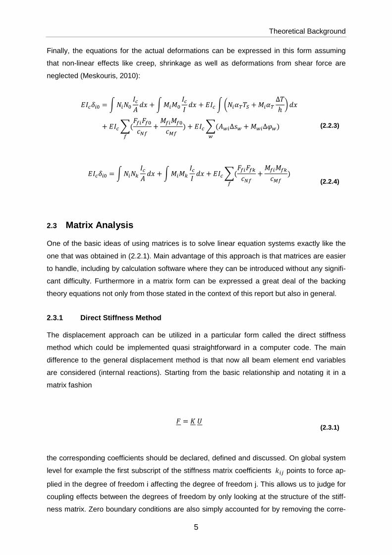
Finally, the equations for the actual deformations can be expressed in this form assuming
that non-linear effects like creep, shrinkage as well as deformations from shear force are
neglected (Meskouris, 2010):
��@��> = +���> �@� -A + +B�B> �@� -A + ��@+C���<D5 +B��< ∆Dℎ F-A+ ��@8(2G�2G>HIG +BG�BG>HJG )G + ��@8(�K�∆$K +BK�∆LK)K (2.2.3)
��@��> = +���9 �@� -A + +B�B9 �@� -A + ��@8(2G�2G9HIG +BG�BG9HJG )G (2.2.4)
2.3 Matrix Analysis
One of the basic ideas of using matrices is to solve linear equation systems exactly like the
one that was obtained in (2.2.1). Main advantage of this approach is that matrices are easier
to handle, including by calculation software where they can be introduced without any signifi-
cant difficulty. Furthermore in a matrix form can be expressed a great deal of the backing
theory equations not only from those stated in the context of this report but also in general.
2.3.1 Direct Stiffness Method
The displacement approach can be utilized in a particular form called the direct stiffness
method which could be implemented quasi straightforward in a computer code. The main
difference to the general displacement method is that now all beam element end variables
are considered (internal reactions). Starting from the basic relationship and notating it in a
matrix fashion
2 = �= (2.3.1)
the corresponding coefficients should be declared, defined and discussed. On global system
level for example the first subscript of the stiffness matrix coefficients ��� points to force ap-
plied in the degree of freedom i affecting the degree of freedom j. This allows us to judge for
coupling effects between the degrees of freedom by only looking at the structure of the stiff-
ness matrix. Zero boundary conditions are also simply accounted for by removing the corre-
Theoretical Background
6
sponding columns and rows from the equation system while the rows terms can be used on
a later stage to evaluate the support reactions.
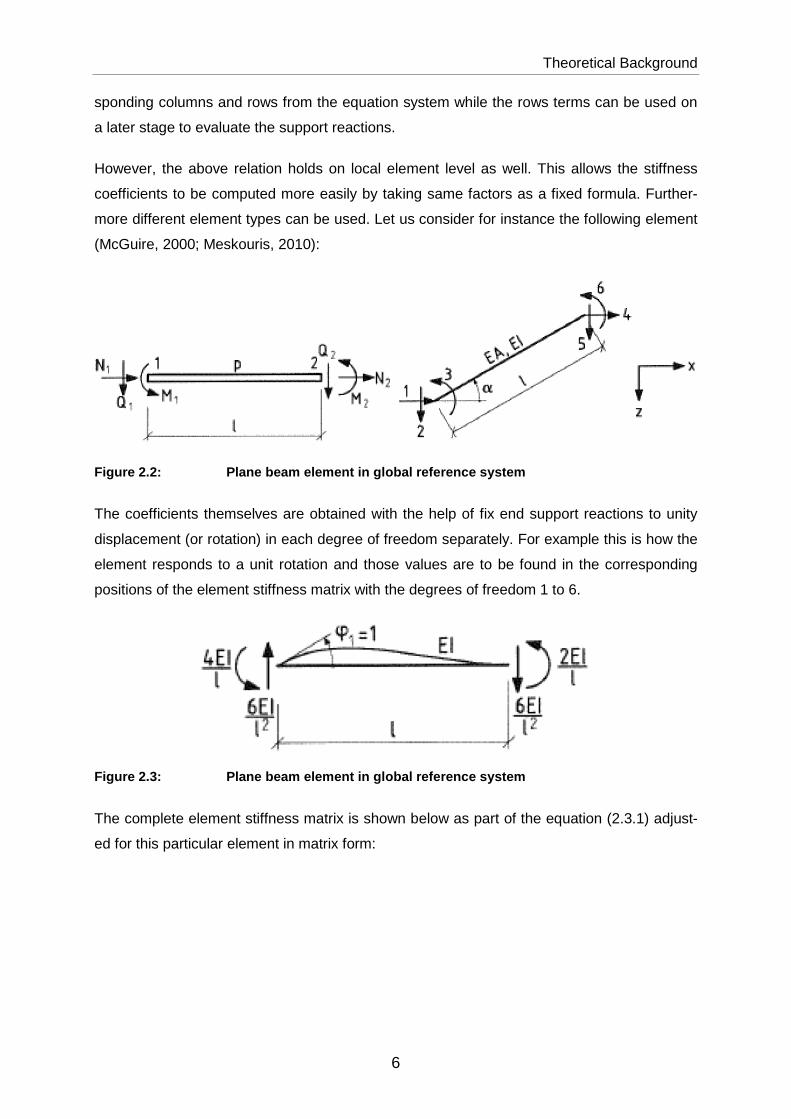
However, the above relation holds on local element level as well. This allows the stiffness
coefficients to be computed more easily by taking same factors as a fixed formula. Further-
more different element types can be used. Let us consider for instance the following element
(McGuire, 2000; Meskouris, 2010):
Figure 2.2: Plane beam element in global reference system
The coefficients themselves are obtained with the help of fix end support reactions to unity
displacement (or rotation) in each degree of freedom separately. For example this is how the
element responds to a unit rotation and those values are to be found in the corresponding
positions of the element stiffness matrix with the degrees of freedom 1 to 6.
Figure 2.3: Plane beam element in global reference system
The complete element stiffness matrix is shown below as part of the equation (2.3.1) adjust-
ed for this particular element in matrix form:

Theoretical Background
7
MNNNNO��P�B���P�B�QRRRRS= ���
MNNNNNNNNNNNO �� 0 00 12�� −6�0 −6� 4
−�� 0 00 −12�� −6�0 6� 2
−�� 0 00 −12�� 6�0 −6� 2
�� 0 00 12�² 6�0 6� 4 QRR
RRRRRRRRRS
MNNNNOV�W�L�V�W�L�QRRRRS
(2.3.2)
2.3.2 Features of the Stiffness Matrix
The above element stiffness matrix is according to the Betti/Maxwell theorem symmetric and
singular with a decrease in the rank of 3 which is exactly equal to the three equilibrium equa-
tions such that the one beam end’s reactions can be expressed with the other end’s ones.
(Meskouris, 2010).
The global stiffness matrix can be studied in order to make conclusions about the well-
posedness of the problem. This is performed with the help of the Lax-Milgam Lemma that by
proving the symmetry and positive definition of the matrix states that the system is well-
posed or uniquely solvable (Sacco, 2013).The global stiffness matrix consists of this kind of
element stiffness matrices that are arranged and overlapped according to the incidence of
local and global degrees of freedom. This happens along the main diagonal of the global
stiffness matrix so that the matrix receives a bandwidth structure where the bandwidth is
equal to the number of nonzero components left and right from the main diagonal term. Es-
pecially when there are a lot of degrees of freedom in the system this bandwidth is small or in
other words there are not many nonzero terms to be found so that the matrix is said to be
sparse or weakly populated. All the zero terms are a sign of uncoupling between the corre-
sponding to the row and column degrees of freedom (McGuire, 2000).
MNNNNNNNO∎ ∎ 0∎ ∎ ∎∎ ∎
⋯ ⋯ ⋯⋱ ⋱ ⋱∎ ⋱ ⋱⋯ ⋯ 0⋱ ⋱ ⋮⋱ ⋱ ⋮∎ ∎ ∎ ⋱∎ ∎ ∎∎ ∎⋱ ⋱ ⋮⋱ ⋱ ⋮∎ ⋱ ⋮
$\�. ∎ ∎ ∎ 0∎ ∎ ∎∎ ∎QRRRRRRRS
Figure 2.4: Typical symmetrical sparse matrix with constant bandwidth = 3

Theoretical Background
8
From computational point of view only the nonzero entries have to be stored in the memory
which decreases the needed space but requires special algorithms to handle the sparse ma-
trix. There are several procedures and modifications of existing methods that exist to opti-
mize the performance of sparse matrices. One of the simplest and fairly common concepts is
to minimize the bandwidth by smartly numbering the global degrees of freedom but also to
exploit the symmetry of the matrix in order to reduce the number of mathematical operations
during the solving phase for maximum efficiency (McGuire, 2000).
2.3.3 Linear Elasticity in Matrix Form
A further example of the successful utilization of the matrix approach is the adaptation of the
Hooke’s constitutive law in matrix form. A separate discussion of the 2D plane strain and
plane stress problems is avoided here as they are not relevant to the current topic. Instead in
order only to illustrate the powerfulness of the matrix approach the formulation of the elastici-
ty matrix for a three-dimensional homogeneous and isotropic material is provided as an ex-
ample (Ghali, 2003):
MNNNNO,1,,̂_`1^`1_`^_QRRRRS = a
MNNNNO�1�^�_�1^�1_�̂ _QRRRRS
(2.3.3)
a = �(1 + )(1 − 2)MNNNNNNNNO(1 − ) (1 − ) (1 − )
0 0 00 0 00 0 00 0 00 0 00 0 0
(1 − 2)2 0 00 (1 − 2)2 00 0 (1 − 2)2 QRR
RRRRRRS
(2.3.4)

Description of Structural System
9
3 DESCRIPTION OF STRUCTURAL SYSTEM
One of the main tasks of the engineer when using software for structural analysis is the ideal-
ization of the real structure to a static model. This, however, is not the main subject of this
report but still deserves the reminder that special attention is required to this aspect. In order
to achieve higher accuracy different element types and different mathematical formulations
are utilized. As we are concentrated on frame structures it could be assumed that for the
purpose of this report the problems begin from an already idealized structural model.
3.1 Geometry
Having in hand such a model the first step to take is to describe its geometry. This can be
fulfilled in the simples manner by assigning a number and x- and y-coordinates to each beam
end point or in other words to each node. The very first matrix in the program – the matrix of
the coordinates provides besides the positioning of each point as a global parameter the
overall number of nodes which is to be used many times in the course of the code.
Departing from the seemingly obvious nodal description of a structure we arrive at the addi-
tional aspects that are of great importance to be considered before entering into other details
of the input like for instance the already mentioned significance of the numbering of the
nodes for the bandwidth of the global stiffness matrix and respectively for the overall compu-
tational speed.
3.2 Topology
As a typical continuous mathematical problem also frame structures has not only geometry
described by position vectors of coordinates but has in addition boundaries with certain
properties and other specifications.
3.2.1 Kinematic Boundary Conditions
The somehow more natural boundary condition is the kinematical one or in other words the
supports that restrain a structure from a kinematic movement. They are sometimes also
called Dirichlet boundaries which can be separated in homogenous and non-homogenous
where the displacement is restrained to a nonzero value or imposed displacement. (Sacco,
2013). For the topology of the model when assigning the matrix of the coordinates this
means that even if on first sight there is no explicit need of defining a node, such must be

Description of Structural System
10
defined in order to allow the further description of the constraints which consists of declaring
the number of the node and the number of the restrained degree of freedom.
3.2.2 Static Boundary Conditions
The second type is the static boundary conditions or simply said the position where a loading
is applied. This is in some way a decision to be made by the user because even if it seems
easier to define a separate node in order to apply a concentrated force there, it is also possi-
ble to consider this force as acting at a certain distance from the beginning of the element.
This on the other hand does not hold for distributed loadings so that in any case the begin-
ning and ending point of this loading must be defined a-priori as individual nodes.
3.2.3 Internal Constraints
Another important issue when defining the nodes is the presence of joints. The algorithm of
master-slave links is employed within the development of this software preferring it to others
such as end releases. The master-slave connection for internal links requires the definition of
two separate nodes with exactly the same coordinates. The role of this will become clear
during the numbering of the global degrees of freedom.
3.2.4 Elements and Incidences
Last but not least each two beam ends must be correctly bound together to form an element.
Two node numbers correspond to each element number whereas it is of importance which of
the nodes is declared first and which second because this is later taken for the element ori-
entation. This plays a role for instance in the stress analysis and bring confusion at the post-
processing or just while looking at the results if the directions of the elements are not clearly
declared a-priori. That’s why some attention is demanded not only to the numbering of the
nodes but also to the consequent construction of this so called matrix of the incidences.
3.3 Cross-Sections
Two other important incidences are regarding to the cross-sections and materials. Each ele-
ment gets an assigned cross-section and material number which leads to specific properties.
The vector of the incidences of the cross-sections stores the information about the cross-
section assignments which has to possess the same length as the total number of elements.
The required section properties for the use of the program are stored in the matrix of the
characteristics of the cross-sections and consist of the area�, the moment of inertia �, the
depth ℎ and the shear correction factor �.

Description of Structural System
11
This allows systems with any number of different cross-sections and materials to be consid-
ered without a great increase in the computational effort in comparison to the by hand calcu-
lations. At this point it is useful to implement an error check for not allowed input values such
as not positive area, moment of inertia or depth which even if taken as unity should be de-
clared as one.
It is interesting to discuss the choice of the area� when accounting �� = ∞ as the code
deals only with finite numbers. A very big value should be chosen but not exaggerated in
order to avoid possible ill-conditioning. This matter is reviewed more detailed in further chap-
ters of this report, including the Benchmarks.
3.4 Materials
In exactly the same way as for the cross-sections functions the vector of the incidences of
the materials. The material parameters required from the program are the modulus of elastic-
ity�, the Poisson’s ratio, the coefficient of thermal expansion α and the specific weight�.
For further use in the program – for the calculation of the element stiffness matrix the relation
between the Poisson’s ratio, the Young’s modulus and the shear modulus � is applied
(Ghali, 2003):
� = �2(1 + ) (3.4.1)
Interesting decision which is made at this stage is the preference for the specific weight�
instead of density�. This is done with the clear thought that this parameter would serve ex-
plicitly for accounting self-weight in which case it is more practical than the density. On the
other hand the density is normally preferred especially when dynamical analysis is performed
which is here not the case. The specific weight can be left zero but should not be negative as
this would not be physically meaningful.
Also in this case it is useful to implement an error check for negative Young’s modulus or
values for the Poisson’s ratio exceeding the limit domain of [-1 0.5]. For the sake of avoiding
unwanted numerical problems it is recommended to nullify the Poisson’s ratio when neglect-
ing shear deformability despite an already chosen great value for the area�.

Numbering of The Degrees of Freedom
12
4 NUMBERING OF THE DEGREES OF FREEDOM
As stated previously the numbering of the degrees of freedom can influence the overall com-
putational efficiency of the program, e.g. by reducing or enlarging the bandwidth of the global
stiffness matrix and therefore the necessary operations during the solving procedure and the
total speed.
4.1 Initialization
The first step is the allocation of the required memory space for the matrix of the degrees of
freedom. In this case the size of the matrix is always equal to [NNODEx3] or in other words
the number of rows is equal to the total number of nodes and the number of columns corre-
sponds to the three degrees of freedom associated with each node. This matrix is in any
case fully populated while during the initialization it is filled with zeroes.
4.2 Restraints and Links
In the second step before the final numbering the restraints and links are being read from the
input file. Each restraint is defined by only one node number and degree of freedom which
means that despite the often case of having one node fully restrained, three separate re-
straints should be declared in the input file. Then each pair of numbers is used as an index of
the matrix of the degrees of freedom with whose help the value in the corresponding position
is set to -1. This would be the only non-positive component of the matrix that will serve as a
mark for the presence of a restraint at this specific position.
Analogous is the input for links which means for instance that for a conventional joint that
allows only relative rotation two entries will be needed and namely stating the master, the
slave node and the degree of freedom. Then according to the master-slave algorithm in the
row corresponding to the number of the slave node and the column corresponding to the
linked degree of freedom is put the number of the master node. This allows in the later num-
bering the same value for the linked degrees of freedom and a different for the non-linked to
be adopted.
4.3 Discretization
In the third step the actual numbering of all degrees of freedom takes place. During the pro-
cedure of populating the matrix it is decided between three different cases as shown below
(Biondini, 2014):
Numbering of The Degrees of Freedom
13
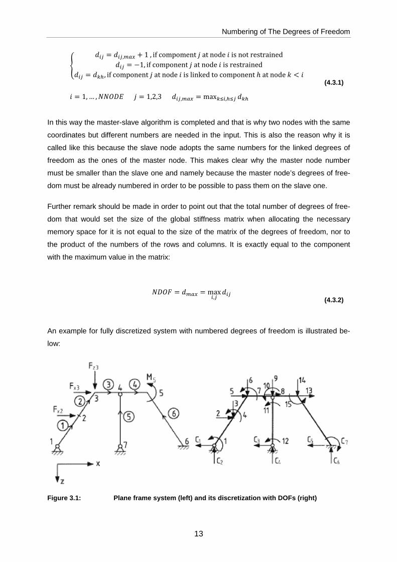
c -�� = -��,de1 + 1, ifcompomentoatnoderisnotrestrained-�� = −1, ifcomponentoatnoderisrestrained-�� = -9u, ifcomponentoatnoderislinkedtocomponentℎatnode� < r r = 1,… ,��za� o = 1,2,3 -��,de1 = max9}�,u}� -9u
(4.3.1)
In this way the master-slave algorithm is completed and that is why two nodes with the same
coordinates but different numbers are needed in the input. This is also the reason why it is
called like this because the slave node adopts the same numbers for the linked degrees of
freedom as the ones of the master node. This makes clear why the master node number
must be smaller than the slave one and namely because the master node’s degrees of free-
dom must be already numbered in order to be possible to pass them on the slave one.
Further remark should be made in order to point out that the total number of degrees of free-
dom that would set the size of the global stiffness matrix when allocating the necessary
memory space for it is not equal to the size of the matrix of the degrees of freedom, nor to
the product of the numbers of the rows and columns. It is exactly equal to the component
with the maximum value in the matrix:
�az2 = -de1 = max�,� -�� (4.3.2)
An example for fully discretized system with numbered degrees of freedom is illustrated be-
low:
Figure 3.1: Plane frame system (left) and its discr etization with DOFs (right)

Nodal Loads in The Global Reference System
14
5 NODAL LOADS IN THE GLOBAL REFERENCE SYSTEM
The here presented computer code is structured in subroutines and until now only the geom-
etry in chapter 3 and the system discretization subroutine in chapter 4 have been discussed.
After these two subroutines, respectively called GEOMET and SCODE, follows the LOADS
subroutine. The complete listing is to be found in the appendix C.
5.1 Input and Initialization
Although this part of the program is subjected to changes each time a new type of loading is
implemented, first it is necessary to describe a core feature that is the minimum required in
order for the program to function. This is namely the presence of loading and especially in its
simplest form as a nodal one.
The input of nodal loads is actually trivial as it requires the specification of the node where
the concentrated force is applied, the direction in which it operates and its amount. At this
point it is useful to indicate that the program utilizes consistent units or in other words the end
user is responsible for the right input of all variables in terms of unit consistency and he/she
must be aware of the particular consistent unit system in order to retain consciousness at the
post-processing phase.
Other important operation at this level is the initialization of the global load vector which will
be later used in solving the final linear system problem. This occurs by allocating the needed
memory space that is for the length of the vector equal to the number of the degrees of free-
dom already computed in the previous subroutine.
5.2 Global Arrangement
After filling with zeroes the global load vector which is also a column vector it is ready to have
values assigned to some of its positions. This takes place directly without the need of any
additional assembling. The possible nodal loads are in the three directions of the degrees of
freedom and are directly globally defined – horizontal positive to the left, vertical positive up-
wards and rotation positive counterclockwise. The corresponding global degree of freedom is
extracted from the matrix of the degrees of freedom with the help of the number of the node
and the direction of the load (1, 2 or 3). Finally the value is put in the position in the global
load vector that corresponds to this global degree of freedom.

Element Properties in The Local Reference System
15
6 ELEMENT PROPERTIES IN THE LOCAL REFERENCE SYS-TEM
Remaining on the topic of loading but changing from global to local reference system there
are still two basic features to be implemented that are fundamental part of each static pro-
gram. Namely the possibility to account for element loads and self-weight. As those kinds of
loading require some special transformations and arrangements they are being accounted
for as a sub-process of the assembling subroutine which will be discussed in chapter 8.
6.1 Equivalent Nodal Force Vector
There are several types of element loadings that can be applied. Most frequently they are
characterized by the order of the polynomial which could describe the shape of the loading.
For instance: constant, linear, quadratic, etc. until nth degree polynomials. Within the context
of this report the first two cases have been developed as the most common ones in praxis.
Higher order loading functions can be then fairly well approximated with a reasonable dis-
cretization of the system.
6.1.1 Sign Convention and Procedure
The strategy to account for continuous loading along the beam element is to properly trans-
form them into nodal forces that are calculated and stored in the so called equivalent nodal
force vector. The equivalent nodal forces are defined as the “Nodal Forces producing the
same effects as the Element Loads in terms of Nodal Displacements s” and are also “the
reversed fixed-end forces” (Biondini, 2014). In local reference system x’-y’ the vector can be
declared as follows where the significance of the variables becomes clearer from the at-
tached illustration (Corigliano, 2005):
3~′ = [��� �̂� ��� ��� �̂� ���]< (6.1.1)
Figure 6.1: Element loading with equivalent nodal f orces. Sign convention

Element Properties in The Local Reference System
16
The actual computation of these terms is conducted by applying the respective loading type
onto a beam member with both ends fixed. The resulting support reactions are then taken
with an opposite sign as coefficients for the components in the vector of equivalent nodal
forces. This is also valid for temperature change which can be uniform or linear.
According to this strategy one is able to implement many different types of loadings respec-
tively to further enrich the current code only by applying the well-known formulas for calculat-
ing the support reactions on a clamped beam as shown in the illustrations below:
Figure 6.2: Beam with both ends fixed
Figure 6.3: Fix end moments according to load case
In the present code cases 1, 3 (also in combination as 2), 4, 6 from the above figure together
with the case of uniformly distributed axial load are implemented (as a remark:� = e� ; � = �� ).

Element Properties in The Local Reference System
17
However, an important difference is to be pointed out when looking at the above formulas
which are intended explicitly for hand calculations. Namely in the presence of unsymmetrical
loading the effect of the shear deformability is observed and although it’s left out for hand
computations, there is no need to neglect it when the computer is employed to perform the
operations. On the example of a uniformly increasing load the influence of the Poisson’s ratio
and shear correction factor are not taken into account by the given formula. In the code on
the other hand the more correct formula derived from the flexibility coefficients using the
force method is implemented:
B� = ���30 �1 + H4� B� = −���20 �1 + H6� H = 12������ + 12���
(6.1.2)
6.1.2 Self-Weight
The principle of superposition of the effects allows the combination of the different load cases
such as the self-weight, distributed loads and temperature change by simply summing all the
contributions. It states that whether applying all loads simultaneously or summing them up
separately, the result remains the same (Ghali, 2003). At this point it is made use of the pre-
viously defined specific weight � by multiplying it with the cross-section area of the element in
order to receive a linear load.
This loading though cannot be added without modifications to the previous contributions as it
acts with difference to the other loadings always in the global reference system, naturally
towards the ground as it is also called gravity load. The necessary transformation is carried
out with the help of the sin and cos of the element orientation angle – the angle between the
beam and the horizontal axis. Multiplying these terms with the self-weight results in transfer-
ring the force from global to the local reference system and also splitting it in part in the direc-
tions of the two local element axes x’ and y’. In this way the linear loading due to self-weight
is added to the other distributed loads in those directions and handled together with them.
These sin and cos terms play an important role for the transformation of coordinates and
when switching between the reference systems in general. This topic is discussed more in
detail in the next chapter.

Element Properties in The Local Reference System
18
6.2 Stiffness Matrix
One of the goals when formulating an element for computational purposes and core part of
the whole program is the formulation of the element stiffness matrix. As it was already men-
tioned in chapter 2.3.1 the stiffness coefficients are obtained usually with the help of the dis-
placement method, except in some cases like for a beam on elastic foundation discussed in
chapter 11. In contrast to the formulation (2.3.2) and similarly to the considerations made in
the previous chapter regarding the shear deformability in hand and computer supported cal-
culations also here those effects are taken into account. Analogous to the Timoshenko beam
finite element bending, shear and axial deformations are being considered in the following
formulation of the stiffness matrix (Ghali, 2003):
�0 =
MNNNNNNNNNNNNO ���0 12��(1 + �)��0 6��(1 + �)�² (4 + �)��(1 + �)�
$\�.−��� 0 00 − 12��(1 + �)�� − 6��(1 + �)�²0 6��(1 + �)�² (2 − �)��(1 + �)�
���0 12��(1 + �)��0 − 6��(1 + �)�² (4 + �)��(1 + �)� QRRRRRRRRRRRRS
(6.2.1)
With
� = 12����²�� (6.2.2)
Perhaps one of the main advantages of this approach is that it is that this formulation is ana-
lytical and the form does not change. What is more all the already discussed in chapter 2
features like the symmetry, the singularity and the significance of the coupling between the
degrees of freedom on local level hold. What remains is to transfer it together with the vector
of equivalent nodal forces from the local to the global reference system and to assemble fi-
nally the global stiffness and load vector for the solving of the linear equation system. This
namely is discussed within the next chapters.

Transformation of The Reference System
19
7 TRANSFORMATION OF THE REFERENCE SYSTEM
7.1 Problem Statement
Elements in a structure are positioned in the global system but for the sake of calculation the
element matrices and vectors one makes use of a local reference system or also sometimes
called element reference system because it facilitates the calculation on element level. This
is due to the fact that the local axis x’ is aligned with the element and the y’ is perpendicular
to it as illustrated below:
Figure 7.1: Beam element in local (left) and global (right) reference system
The goal in this situation is to make all matrices computed on element level valid also for the
whole structure. This is achieved mainly with the help of the angle � as shown on the right in
the above figure.
7.2 Transformation of 2D Coordinate System
In more general sense the transformation of a beam element corresponds to a coordination
transformation for example of a continuous linear element in the mathematics where there is
absolutely no mechanical meaning of the procedure. As already stated the key to solving the
problem is the angle � which allows through trigonometric relationships to calculate the two
projections of the inclined element, respectively of the inclined local system with respect to
the global one and vice versa. This is achieved with the simple geometrical relations coming
from the definition of the sin and cos trigonometric functions as shown in the following figure:

Transformation of The Reference System
20
Figure 7.2: Sin and cos relations
Analogously these relations are used to form the axes transformation equations that for the
case of x-y-z global and x’-y’-z’ local coordinate systems look like this Schnepp, 2012):
�A = H�$�A� − $r��\′\ = $r��A� + H�$�\′� = �′ (7.2.1)
7.2.1 2D Beam Element Transformation Matrix
Adopting these equations and reformulating them in a matrix form the transformation matrix
of a point is constructed. As the beam element exactly like the general continuous linear el-
ement has two points – starting and ending this matrix is to be repeated in order to compile
the final element transformation matrix as illustrated in the following expressions (Schnepp,
2012):
D> = �H�$� −$r�� 0$r�� H�$� 00 0 1� (7.2.2)
D = �D> | 0− + −0 | D>� (7.2.3)
7.2.2 Features and Application of the Transformatio n Matrix
There are two main features of the transformation matrix, namely the orthogonality and the
normality that are expressed respectively in the following relations (Schnepp, 2012):

Transformation of The Reference System
21
D�� = D⇔DD< = D<D = � (7.2.4)
-��D = 1 (7.2.5)
The transformation matrix is used for all three members of the linear equation system formu-
lated on the element level�′$′ = 3′. As the transformation matrix is formulated in geometrical
sense for vectors it is possible to simply replace $′ = D<$ and3′ = D<3. Doing this leads us to
the following expression then pre-multiplied on both sides with the matrix D in order to obtain
the relation for the matrix � (Biondini, 2014):
�′D<$ = D<3
D��<����� $ = DD<3 = 3 (7.2.6)
In this way all components can be transferred between the reference systems at any time.
This can be particularly useful in the post-processing phase and that is why it is stored to-
gether with each element’s stiffness matrix and load vector in a temporary file used later dur-
ing the stress analysis in the subroutine STRESS as shown in chapter 10. The complete
structure can be found in appendix A of the report.

Structural Assembly
22
8 STRUCTURAL ASSEMBLY
In the previous two chapters were described operations that take place as a sub-process
(MKK) of the assembly subroutine ASSEMB. The main significance is that those steps are
performed for each element subsequently in order to receive the individual contributions to
the global stiffness matrix and global load vector. The task of the assembly procedure is to
correctly put together all these contributions.
The first step is to initialize the global stiffness matrix. It is quadratic with the number of col-
umns and rows equal to the total number of degrees of freedom in the structure.
8.1 Assembly Matrix
One of the options to achieve the right positioning is with the help of an assembling matrix.
This is actually a Boolean matrix – a logical matrix that consists only of ones and zeroes. The
size is exactly the same as the size of the already allocated global stiffness matrix but it is
computed and used for each single element separately in an analogous manner to the trans-
formation matrix. What makes this approach computational inefficient is that in contrast to the
transformation matrix the assembly matrix is not 6x6 matrix but much larger and extremely
weakly populated and a matrix operations are to be carried out not only once as with the
stiffness matrix but for each element. These operations correspond otherwise exactly the
multiplication carried out with the transformation matrix as shown below for element� as
part of system with� degrees of freedom (Biondini, 2014):
��)1) = �d�)1��d��1� �d<��1) (8.1.1)
8.2 Direct Assembly
The most commonly implemented algorithm nowadays in commercial codes is the direct as-
sembly. For each element with the help of their incidences are extracted the node numbers.
Then there are two options to compute the indices that are needed to place in their position
in the global matrix the local contributions depending on the programmer’s choice. Either a
formula is exploited that for each indexr = 3( − 1), where is the node number, or as in the
present case the global degrees of freedom corresponding to each node are extracted from
the matrix of the degrees of freedom and they represent the needed indices. By summing the

Structural Assembly
23
individual contributions moving along the main diagonal the bandwidth scheme of the matrix
is created. An illustrative example is shown in the figure below:
Figure 8.1: Example for global stiffness matrix wit h assembling steps
Looking at a global stiffness matrix there are a few statements that can be made. Let us take
the above on for instance. Being a 9x9 matrix with summation of terms on a 3x3 space in its
center and knowing that each element has a 6x6 element stiffness matrix leads to the con-
clusion that the overall structure consists of two elements that are connected together in the
middle. In other words it is clear that the degrees of freedom of the first beam’s end coincide
with the degrees of freedom of the second one’s end and are the global 4, 5 and 6. Even for
small system like this a bandwidth structure is recognizable, which is a natural result of the
complete uncoupling of the not connected beam ends of the two elements.
Having constructed the global stiffness matrix and global load vector, it can be processed
further to the solving procedure.

Solution of The Linear System
24
9 SOLUTION OF THE LINEAR SYSTEM
The first step is to establish an appropriate method for solving the system. Basically the prob-
lem to be solved is the following:
�$ = 3 ⇔ $ = ���3 (9.1.1)
The inversion of the matrix is the computationally most costly procedure and for instance a
direct inversion is not advisable.
9.1 Gauss Elimination Method
Other solution methods are divided in direct elimination and iterative methods with their ad-
vantages and disadvantages regarding mainly speed and accuracy. For the purpose of the
current development Gauss elimination method has been chosen as one of the standard
approaches also in many commercial codes that make use of the equivalence theorem for
linear equation systems. The main goal is to achieve a triangular structure of the matrix � by
simple divisions and subtractions of the equations by the main diagonal terms so that finally
all the unknown displacements can be received by substituting one at a time starting from the
very last row where only one unknown has remained. In other words the Gauss method con-
sists of two main parts that are formulated in the following expressions regarding the linear
system �A = ¡¢r�ℎ( = [�|¡] and their equivalent terms with tilde and with small letters
stating the matrix coefficients (Biondini, 2014):
1. Forward elimination
£ ¢¤�9 = ¢�9¢��¢¤�9 = ¢�9 −¢�9¢�� ¢��, r = 1,… , � − 1, o = r + 1,… , �, � = r, … , � + 1
(9.1.2)
2. Backward substitution
A� = ¡¥� − ∑ §̈�9A9)9;�©�§̈�� = ¡¥�� − 8 §̈�9A9)9;�©� , r = �,… ,1
(9.1.3)
Solution of The Linear System
25
This formulation is actually called the compact procedure which introduces an improvement
to the basic one by performing the equation subtraction with a coefficient divided by the cor-
responding main diagonal term so that at the end of the elimination procedure a triangular
structure is obtained with only ones at the main diagonal. This saves one division operation
at each cycle during the backward substitution. In this way round-off errors are reduced be-
cause the numbers during the backward substitution have more similar magnitude in com-
parison to the basic procedure. Furthermore, by the number of N of multiplications/divisions
needed to perform the elimination procedure it can be judged about the computational effi-
ciency of the two modifications of the Gauss method (Biondini, 2014).
��eª�@ ≈ 2��3 + C3�2 − 1F�� + C13 −�2F�
�@¬de@* ≈ ��3 +��� − �3 (9.1.4)
Where � states the number of equations and � the number of constant term vectors. Taking
a look at the coefficients in front of the 3rd and 2nd grade terms one can notice the difference
between the two modifications. Even for a few equations the compact procedure is more
efficient and this tendency grows further with the increase of the number of equations. Other
options are among other the Cholesky and the root-free method that are more reasonable for
very large systems. Other improvements involve exploitation of the symmetry and the band-
width of the stiffness matrix but also higher complexity.
9.2 Conditioning of the Linear Equation System
As already mentioned not only the speed of the solution is of importance but also the accura-
cy. Numerical errors occur depending on the precision used to represent the numbers (trun-
cation) and on the implemented algorithm which can compensate or accumulate truncation
errors (round-off errors).
The accuracy of the solution on the other hand depends on the conditioning (sensitivity of the
function to be evaluated) and the stability of the algorithm where the latter is not influenced
by the function but by the hardware and software. The relevant parameter that should be
controlled is the conditioning of the system which states if small variations are being boosted
and have great influence on the result or on the contrary are being compensated so that the
system remains stable. One speaks of ill-conditioned and well-conditioned systems(Cook,
2002).

Solution of The Linear System
26
9.2.1 Evaluation of Condition Number (a-priori)
The goal of an error test is to estimate the error in the solution without knowing the exact
solution. However, with the help of some mathematical operations the following inequality
has been proven(McGuire, 2000; Biondini, 2014):
‖∆$‖‖$‖ ≤ ‖�‖‖���‖�°°�°°�@¬)±(�)‖∆3‖‖3‖
(9.2.1)
‖∆$‖‖$‖ ≤ H��-(�)1 − H��-(�) ‖∆G‖‖G‖ (‖∆3‖‖3‖ + ‖∆�‖‖�‖ ) ≈ H��-(�)(‖∆3‖‖3‖ + ‖∆�‖‖�‖ ) (9.2.2)
In this inequality only the left-hand-side is unknown because in the brackets on the right the
internal precision used by the program is inputted because the∆ terms stay for purely trunca-
tion errors. Conducting some additional operations a final statement is reached based only
on the condition number H��-(�) for the maximum number of significant digits that could be
lost in the solution process�:
� = log[H��-(�)] (9.2.3)
Due to the fact that this formula contains a logarithm it becomes obvious that a high accuracy
in computing the condition number is not required. Finally, the equation for the condition
number makes use of the Euclidian matrix norm and its possibility to be found by the maxi-
mum or minimum eigenvalues of the matrix in a way that replaces the need of inverting the
stiffness matrix with the necessity to solve the eigenvalue problem to find the minimum and
maximum eigenvalue. As a remark concerning the code is that a complete subroutine for
finding the eigenvalues according to the Jacobi method is adopted from (Press, 1992):
H��-�(�) = ‖�‖�‖���‖� = ³de1³d�) (9.2.4)

Solution of The Linear System
27
9.2.2 Diagonal Decay Error Test (in-progress)
Although the condition number provides the most accurate estimation of the error in the solu-
tion, the in-progress diagonal decay error test is also implemented as it is much less complex
and together with the posteriori test provides additional security about the quality of the re-
sult. This approach is directly integrated in the Gauss elimination procedure and uses the
diagonal ith term of the original matrix ��� and the term �´µ́ just before the elimination of the ith
degree of freedom. At the end the whole approach can be summarized in those steps where
at the second one the factor � is the same as for the condition number (Cook, 2002):
�� = ����´µ́ = 10d (9.2.5)
0 ≤ � ≤ 23 ≤ � ≤ 9� ≥ 10 ¢��� − H��-r�r���-$\$��� �$$r¡����-���r�� ¸�¡���r�� − H��-r�r���-$\$���
(9.2.6)
9.2.3 Work of Residuals (posteriori)
Another simple error test is the posteriori method through the work of residuals which is ad-
visable to be implemented together with the other two for maximum quality control of the so-
lution. After passing them the convergence of the solution is assured. In this method only one
single factor is evaluated and namely the ratio between the work of residuals ∆3 and the
work of loads3. In both cases the already computed solution is used and the residuals com-
puted through backward multiplication of the obtained solution with the stiffness matrix are in
a weighted manner compared with the actual load vector (Biondini, 2014; Cook, 2002):
�¹ = ∆(( = $̃<∆3$̃<3 (9.2.7)
�¹ ≤ 10�»�¹ ≥ 10��
¢��� − H��-r�r���-$\$��� �$$r¡��r�� − H��-r�r��r��
(9.2.8)

Stress Analysis
28
10 STRESS ANALYSIS
Once obtained the solution in terms of displacements it remains important to conduct the so
called stress analysis as a second essential part of the useful set of results. At this level one
is entering into the post-processing phase to which has been referred already a couple of
times during the report.
10.1 Sign Convention
Starting from the input stage it was stressed the importance of retaining the overview over
the elements orientation. This is important because of the fact that there are two different
sign conventions for the internal reactions and for the element nodal forces. For instance the
signs for the axial force and bending moment coincide at the end of the beam, but for the
shear for at the beginning. This is graphically explained in the following figure (Corigliano,
2005):
Figure 10.1: Sign convention for element nodal forc es (left) and internal reactions (right)
The stress analysis is tightly bounded with the previous calculations that took place on ele-
ment level before the solution of the problem or in other words with the stiffness matrix, the
transformation matrix and of course the vector of equivalent nodal forces.
10.2 Internal Reactions
These three element matrices were written aside in a temporary file for each element to be
able to be used exactly at this stage. There are a few different options to calculate the inter-
nal reactions within the elements and in the current code is implemented the one that is utiliz-
ing the element matrices calculated before to construct the equilibrium equation with the al-
ready known displacements.

Stress Analysis
29
The first step is to extract the corresponding to each element nodal displacements. As they
are stored in global coordinates it is necessary to apply the transpose transformation matrix
to transfer them to the local coordinate system. Then the equilibrium equation�$ = 3 is eval-
uated for all six degrees of freedom of the element or for three degrees of freedom of each
node.
The second possibility is based on equilibrium between the internal reactions, the equivalent
nodal forces and the acting loading without using the element stiffness matrix. Instead a set
of formulas is developed as shown below while keeping in mind the notations and signs from
Fig. 10.1 (Corigliano, 2005):
¼½½½¾½½½¿ �(A�) = −�� −+ 1(À)-À1�
>D(A�) = �� ++ ^(À)-À1�
>B(A�) = −�� + ��A� ++ ^(À)À-À1�
>
(10.2.1)
¼½¾½¿ �(A�) = −�� − 1A′D(A�) = �� + ^�A� + ( ^� − ^�) A′²2�B(A�) = −�� + ��A� + ^� A��2 + ( ^� − ^�) A′³6�
(10.2.2)
The third possibility which is actually more common for finite element codes is based on the
linear elastic constitutive law together with a kinematic hypothesis for the displacement-strain
relationship. In this way from the displacement filed one can obtain the strain tensor through
for example a deformation gradient and then express the desired stress tensor which can be
further integrated to obtain the internal reactions (Schnepp, 2012). This approach involves
lower accuracy and higher complexity so that is why it is used mainly in the cases where
formulating the equilibrium is not possible or nearly impossible like for instance for plate and
shell elements.

Specialized Problems
30
11 SPECIALIZED PROBLEMS
Until now studied topics have covered only the main features that are normally expected -
the core of this kind of software. In this chapter a few additional features are introduced.
11.1 Prestressing
First of these features here will be discussed the prestressing as it is a part of the concrete
structural design that has been gaining significance for the last decades. Before going into
detail about the practical application in terms of computer code it is important to clarify the
main concept of prestressing.
11.1.1 Basic Principle and Technology
The fundamental idea behind the prestressed concrete members is to achieve a stress state
in the end configuration such that the tensile stresses on the concrete surface vanish. This is
accomplished by balancing out the prestressing forces with the external loading and is espe-
cially practical for carriers where tensile stresses are expected. Figuratively it can be seen in
the following illustration (Will, 2012):
Figure 11.1: Stresses resulting from prestressing, constant and variable external load-ing
The production process of the prestressed members influences the characteristics, the per-
formance and in this way also the actual calculation procedure, so it is necessary to point out
the main techniques. They are divided mainly in pre-tensioning, post-tensioning, external
prestressing and prestressing with or without compound. Manufacturing procedures are
demonstrated through images (Will, 2012):

Specialized Problems
31
Figure 11.2: Production procedure with pre-tensioni ng in prestressing bed
More complex tendon layouts are accomplished through redirecting the tendon and in gen-
eral the post-tensioning technique offers better possibilities. For the post-tensioning case the
prestressing jack is put into function after the placement of the concrete which then supports
the redirecting of the tendon to the final layout. Schematically departing from the above figure
one can exemplify the mechanism in the following way:
Figure 11.3: Tendon redirection (with post-tensioni ng)
The high tensile steel wires are placed in usually plastic sleeves which can be filled with
grout or not, respectively differentiating between tendons with and without compound. The
grout can be placed before the installation of the concrete in the pre-tensioning case or it can
be injected later during the post-tensioning. The purpose of the grout and the sleeves is to
reduce the contact concrete-steel contact and in this way to minimize the friction losses (Will,
2012).
11.1.2 Prestressing Losses
Namely the losses caused by different effects are one main aspect within design of pre-
stressing members. They can be divided in two major groups: time-dependent or delayed
and time-independent or immediate, while restricting the discussion from the losses during
and caused by the production mechanism and equipment. The time-dependent effects are
creep, shrinkage and relaxation and they are difficult to be preciously calculated because of

Specialized Problems
32
their non-linearity and dependency on a series of factors among other the production tech-
nology, the materials involved, the cross-section of the beam and the loading (except for
shrinkage) of the system. Usually these losses are accounted for by adopting fixed factors
provided from the national construction norms.
Friction losses on the other hand can be estimated based on analytical knowledge. Many
factors still play a role such as the redirecting, the glide slope, surface, clamping actions or
the tendon sleeve. However, it is still possible to formulate equilibrium and to utilize the fric-
tion formula of Coulomb – Couley as illustrated below:
Figure 11.4: Equilibrium for friction losses accord ing to Coulomb - Couley
Based on this drawing one can formulate and solve a differential equation that leads to the
final expression for the prestressing force in general and in the post-tensioning case (11.1.2)
that depends on the friction coefficientÁ and the tendon curvature� (Will, 2012):
 = Â> ∙ ��ÃÄ(1) (11.1.1)
∆ÂÃ(A) = Â>(1 − ��Ã(Å©91)) (11.1.2)
Having stated the different types of prestressing losses it is important to emphasize the fact
that those losses are neglected in the course of the current software development. Instead a
constant prestressing force is assumed.

Specialized Problems
33
11.1.3 Implementation
Despite the inaccuracy of the assumption for constant prestressing force reasonable results
can still be achieved with the help of programmatic techniques. In this way it can be account-
ed for losses and arbitrary profiles by constructing a mesh with a sufficient density or in other
words by enough subdivisions of the elements in order to minimize the error.
As it can be considered strictly as a loading case the prestressing requires changes on ele-
ment level in the vector of the equivalent nodal forces and during the stress analysis of the
internal actions. A particularity of the prestressing element is that it represents a self-
equilibrating load system and uses a different sign convention with respect to the other load-
ing conditions. Otherwise the principle of superposition still holds which allows also the
summation of the element equivalent nodal forces due to the balancing load coming from the
curvature of the tendon (similar to the case in Fig. 11.4) and the anchorage end forces. The
formulas, graphical explanation and sign convention are clarified below:
Figure 11.5: Prestressing element in local referenc e system
3~′ = 3~′e + 3~′� = ÂMNNNNNNNNO 1− �� − ���13 (−2�� + �� − 2�d)− − −−−−−−−−−1�� − ���− 13 (�� − 2�� − 2�d) QR
RRRRRRRS
(11.1.3)
Another issue is the way to consider multiple tendons. One possibility is to define in the input
phase a three dimensional matrix which would be the most accurate option but is unfortu-
nately computationally ineffective. The other option is to implement the so called equivalent
tendon. Its idea is that all input data is summarized as a weighted average so that correct

Specialized Problems
34
calculations can be carried out with this only one average tensor. The formula utilized for this
purpose reads as follows:
�(A�) = 1Â8Â���(A�))�;�
(11.1.4)
11.2 Elastic Constraints and Links
Another essential feature of the program is the presence of elastic constraints and links or in
other words – springs. They can be used as restraints or as internal constraints. The main
difference between the two situations is the manner in which the spring stiffnesses contrib-
utes to the global stiffness matrix. In the case of constrained or also denoted in some
sources Robin boundary condition (Sacco, 2013) only one degree of freedom is affected
while in the case of elastic link two degrees of freedom are coupled by a single spring. The
two situations are illustrated in the following sketch:
Figure 11.6: Elastic restraint (left) and link (rig ht)
The spring can be handled as a separate element type with a stiffness matrix which contribu-
tions are being assembled in a similar way as the beam element stiffness matrix. For this
purpose a separate subroutine JOINTS is introduced that handles also imposed displace-
ments. There is also not a significant difference between displacement and rotational springs
as numerically it is still the stiffness coefficient�@: �ª��)Æ = �@ Ç 1 −1−1 1 È (11.2.1)

Specialized Problems
35
11.3 Imposed Displacements
A common load case in the praxis could be foundation settlement which represents an abso-
lute imposed displacement. In addition to this case in the current code relative displacements
are taken into account.
11.3.1 Absolute Displacements
When applying for instance support settlement the corresponding degree of freedom is set
free and forced to obey not equilibrium but compatibility condition. The effect can be repro-
duced by applying equivalent nodal forces3~ at the degree of freedom:
3~� = −���$̅� (11.3.1)
By this means additional equation(s) is introduced to the linear system. This, however,
changes the size of the overall problem and thereby harming the computational efficiency of
the algorithm because the global stiffness matrix loses its quadratic form and symmetry. The
idea used to address this issue is not to introduce but to replace an equation in the linear
system and namely an equilibrium one with a compatibility one. Through some mathematical
operations not only the global stiffness matrix remains quadratic but also symmetric. This is
achieved through setting to zero all the row and column terms corresponding to the degree of
freedom to zero except for the main diagonal term which usually is left unchanged in order to
avoid ill-conditioning. Then all the column terms are being subtracted from the global load
vector so that the solution is not affected.
11.3.2 Relative Displacements
Coming from its name the relative displacement describes the final displacement which is the
result of two separate degrees of freedom at the same place that is to say at joint connec-
tions. Analogously to the previous case also here compatibility equations are utilized but an
internal equality of the reaction forces of the connected degrees of freedom plays a role.
Thereby the complexity of the problem is increased which is natural because of the presence
of two instead of one degree of freedom which results in additional mathematical operations.
Despite this the goal remains the same and namely to maintain the symmetry of the global
stiffness matrix. The starting equation system includes the already mentioned reaction forces
and starting from there the row and column corresponding to one of the degrees of freedom
is being nullified except for three terms that are at the coupling positions between these de-

Specialized Problems
36
grees of freedom and on the main diagonal. Before doing this the row and column terms are
being added to the row and column of the other degree of freedom whereas the column
terms are also added to the load vector. At this point the reaction forces are being eliminated
from the system.
11.3.3 Inclined Constraints
The last function performed in the subroutine JOINTS is regarding to the global orientation of
until now discussed elastic constraints and imposed displacements. Let us consider a set-
tlement at inclined roller support. By definition the roller acts in one degree of freedom but its
inclination with respect to the global system induces the projection from one local axis of the
roller to the two global axes. This issue is similar to the transformation between local and
global system on element level but in this case there is no element. Still a local transfor-
mation matrix could be utilized by arranging it on the right positions in a global transformation
matrix which would be equal the identity matrix of size of the number of the degrees of free-
dom in the system if there were no inclined constraints. It is, however, more efficient not to
perform matrix multiplication on global level with extremely weakly populated matrices. In-
stead of this a procedure similar to the direct assembly is implemented along with the coordi-
nate transformation equations. The expressions are not exactly the same as formulated in
(7.2.1) because in this case they are applied on the global linear system not in matrix form.
But keeping in mind the expression � = D��D< one can understand that those transfor-
mations terms are utilized in different fashion for the different terms of the stiffness matrix
depending on the region where they are situated.
11.4 Elastic Foundation
An interesting programmatic possibility especially from geotechnical point of view represents
the Winkler’s model for a beam element on elastic foundation that is intended to idealize in a
better way the characteristics of the soil:
Figure 11.7: Beam element on elastic foundation
The behavior of this beam element can be divided in axial and flexural for the plane situation
and an additional torsional part when operating in the three dimensions. The stiffness coeffi-
cients are then obtained separately for the different behaviors. For the sake of simplicity the

Specialized Problems
37
force method is preferred to the displacement in contrast to the Timoshenko beam and
thereby through the flexibility coefficients receiving the flexibility matrix�. Finally, the rela-
tionship is exploited stating that:
� = ��� (11.4.1)
The vector of equivalent nodal forces may be also computed based on the force method ap-
plied to the fixed-end beam with the corresponding loading such that in correspondence with
(11.4.1) leads to the final equation (11.4.3):
��3>′ + �>′ = 0 (11.4.2)
3~′ = −3>′ = �′�>′ (11.4.3)
Due to the fact that an entirely new element type is being implemented some changes are
necessary in different levels of the program that are though still not too drastic. Apart from
the elastic bedding properties in the input phase new incidence should be introduced to show
the beam type of each element, e.g. 0 for Timoshenko and 1 for Winkler beam. One must
then check this value during the assembly procedure and call the corresponding subroutine
for calculating the element matrices, again - MKT for Timoshenko and MKW for Winkler.
Once obtained the stiffness contributions to the global stiffness matrix and load vector, the
rest of the procedures remain practically the same. At this level we restrain ourselves from
further increase the capacity of the program by introducing for instance rigid joints, offsets or
elements with varying cross-sections. Therefore being this the last enhancement of the pro-
gram within this report, its correctness is still to be validated based on many various bench-
marks presented in the next chapter.
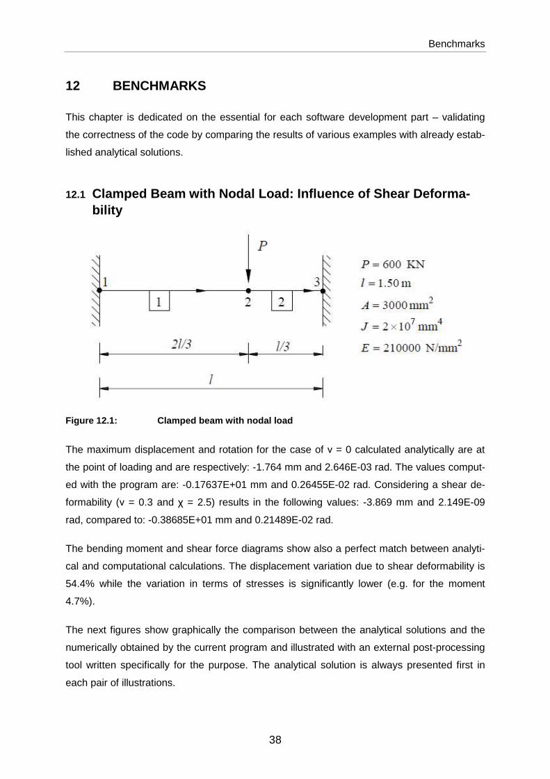
Benchmarks
38
12 BENCHMARKS
This chapter is dedicated on the essential for each software development part – validating
the correctness of the code by comparing the results of various examples with already estab-
lished analytical solutions.
12.1 Clamped Beam with Nodal Load: Influence of Shear De forma-bility
Figure 12.1: Clamped beam with nodal load
The maximum displacement and rotation for the case of ν = 0 calculated analytically are at
the point of loading and are respectively: -1.764 mm and 2.646E-03 rad. The values comput-
ed with the program are: -0.17637E+01 mm and 0.26455E-02 rad. Considering a shear de-
formability (ν = 0.3 and χ = 2.5) results in the following values: -3.869 mm and 2.149E-09
rad, compared to: -0.38685E+01 mm and 0.21489E-02 rad.
The bending moment and shear force diagrams show also a perfect match between analyti-
cal and computational calculations. The displacement variation due to shear deformability is
54.4% while the variation in terms of stresses is significantly lower (e.g. for the moment
4.7%).
The next figures show graphically the comparison between the analytical solutions and the
numerically obtained by the current program and illustrated with an external post-processing
tool written specifically for the purpose. The analytical solution is always presented first in
each pair of illustrations.

Benchmarks
39
Figure 12.2: Deformed shape: Clamped beam with noda l load
Figure 12.3: Shear force diagram: Clamped beam with nodal load

Benchmarks
40
Figure 12.4: Bending moment diagram: Clamped beam w ith nodal load
12.2 Frame with Uniform Temperature Change
The following frame consists of two bars with EA = ∞, different moments of Inertia, fully
clamped at their ends and subjected to uniform temperature change ∆T = 20°C. With input
value for A = 1E10 mm² the analytical and numerical results are again the same.
Figure 12.5: Frame with uniform ∆T

Benchmarks
41
Figure 12.6: Deformed shape: Frame with uniform ∆T
Figure 12.7: Axial force: Frame with uniform ∆T

Benchmarks
42
Figure 12.8: Shear force: Frame with uniform ∆T

Benchmarks
43
Figure 12.9: Bending moment: Frame with uniform ∆T
12.3 Frame with Pinned Joints and Foundation Settlement
The following frame has its left column clamped and the right as jointed support with 9 mm
settlement. Shear deformability is again not considered, the columns have different moments
of inertia while the right is connected to the above structure with a link. The system is also
subjected to a constant load in vertical direction:
Figure 12.10: Frame with Pinned Joints and Foundati on Settlement

Benchmarks
44
Figure 12.11: Deformed shape: Frame with Pinned Joi nts and Foundation Settlement
An interesting aspect is that this system is more sensible to very big values of the cross-
section area A. Correct results are obtained with A = 1E6 until ca. 1E12 but with greater val-
ues the solution may become instable due to numerical problems and ill-conditioning. For
example by exaggerating the value for A = 1E25 we obtain max Ux = -2.994E+00 and max Uy
= -2.194E+01. This for the horizontal displacement is an error in the order of 10. The analyti-
cal solution for rotation at the upper left corner is -4.514E-03 rad compared to -0.41538E-02
rad computed with A = 1E12 mm² and -0.41620E-02 rad with A = 1E6 mm².
Greater values increase of A or I the accuracy when EA = ∞ or EI = ∞ but to avoid with cer-
tainty any ill-conditioning a rule of thumb is to pick such values that the following relations are
approximately satisfied:
��Ê ⩰ 1�6 (12.3.1)
��ʳ ⩰ 1�6 (12.3.2)

Benchmarks
45
Figure 12.12: Axial force: Frame with Pinned Joints and Foundation Settlement

Benchmarks
46
Figure 12.13: Shear force: Frame with Pinned Joints and Foundation Settlement
Figure 12.14: Bending moment: Frame with Pinned Joi nts and Foundation Settlement

Benchmarks
47
The maximum value for the bending moment differs a little from the analytical one but in this
case this is due to an interpolation error during the post-processing. The reason for that is
that the exact position of the maximum moment was not specified a-priori. The variation re-
mains negligible: (142.269-141.854)/142.269*100 = 0.29% < 0.5%.
12.4 Frame with Elastic Restraints and Linear Differenti al Tempera-ture Change
The following frame is constrained at all its ends. To the left it is constrained by rotational
spring, to the top by clamped shear force joint and to the bottom by a roller connected to a
horizontal spring. Also in this case shear deformability is neglected and the horizontal bar
has a different moment of inertia. It is also subjected to a linear differential temperature
change ∆T = 10°C across a 500 mm depth.
Analytically determined relation between the maximum and minimum relation of the structure
(at left and right ends of the horizontal bar respectively) is ⩰ 1.14. Computed by the program
rotations are 0.45775E-03 and -0.40213E-03 which results in a factor of 1.1383 ⩰ 1.14.
Figure 12.15: Frame with elastic restraints and lin ear ∆T

Benchmarks
48
Figure 12.16: Deformed shape: Frame with elastic re straints and linear ∆T
Figure 12.17: Axial force: Frame with elastic restr aints and linear ∆T

Benchmarks
49
Figure 12.18: Shear force: Frame with elastic restr aints and linear ∆T

Benchmarks
50
Figure 12.19: Bending moment: Frame with elastic re straints and linear ∆T
12.5 Portal Frame with Inclined Roof Beams and Tie Rod
The following frame has two jointed supports and a tie rod connected with links to the rest of
the system which is subjected to constant vertical load onto the inclined roof beams.
Figure 12.20: Frame with inclined roof beams and ti e rod

Benchmarks
51
Figure 12.21: Deformed shape: Frame with inclined r oof beams and tie rod
Figure 12.22: Axial force: Frame with inclined roof beams and tie rod

Benchmarks
52
Figure 12.23: Shear force: Frame with inclined roof beams and tie rod

Benchmarks
53
Figure 12.24: Bending moment: Frame with inclined r oof beams and tie rod
12.6 Two Frame Systems Subjected To Various Loads
Figure 12.25: The two frame systems without loading
The Input is L = 6, H = 4, I1 = 0.4, I1 = 0.9, I1 = 1.1, EA = ∞. For the constant load cases the
amount is 5 and for the concentrated 15. In the next tables the comparisons between analyti-
cal (A) and computational (C) results are illustrated. The load cases are described as follows:
1. LC1, Sys 1 – constant vertical load on the upper bar
2. LC2, Sys 1 - constant horizontal load on the left bar
3. LC3, Sys 1 – concentrated horizontal load in point B
4. LC1, Sys 2 – constant vertical load on the upper bar
5. LC2, Sys 2 – concentrated vertical load in the middle of the upper bar

Benchmarks
54
6. LC3, Sys 2 – concentrated horizontal load in point B
MA MB MC MD Mmax VA VD HA HD
A -6.5323 13.0645 13.0645 -6.5323 -9.4355 -15.00 -15.00 -4.8992 -4.8992
C -6.5323 13.065 13.065 -6.5323 -9.4355 -15.00 -15.00 -4.8992 -4.8992
Table 12.1: Results comparison: LC1, System 1
MA MB MC MD HA HD
A 20.5183 -3.8366 4.6968 -10.9484 16.0887 -3.9113
C 20.518 -3.8366 4.6968 -10.948 16.089 -3.9113
Table 12.2: Results comparison: LC2, System 1
MA MB MC MD VA VD HA HD
A 20.40 -9.60 9.60 -20.40 3.20 -3.20 -7.50 7.50
C 20.40 -9.60 9.60 -20.40 3.20 -3.20 -7.50 7.50
Table 12.3: Results comparison: LC3, System 1
MA MB MC MD Mmax VA VD
A -0.81346 9.8632 9.8632 -0.81346 -12.6368 -15.00 -15.00
C -0.81346 9.8632 9.8632 -0.81346 -12.637 -15.00 -15.00
Table 12.4: Results comparison: LC1, System 2
MA MB MC MD Mmax VA VD
A 0.61009 -7.3974 -7.3974 0.61009 15.1026 7.50 7.50
C 0.61009 -7.3974 -7.3974 0.61009 15.103 7.50 7.50
Table 12.5: Results comparison: LC2, System 2
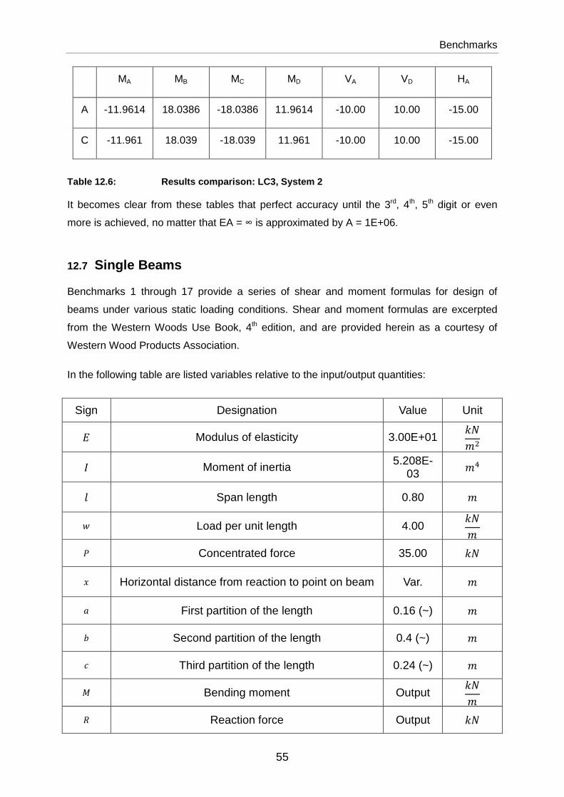
Benchmarks
55
MA MB MC MD VA VD HA
A -11.9614 18.0386 -18.0386 11.9614 -10.00 10.00 -15.00
C -11.961 18.039 -18.039 11.961 -10.00 10.00 -15.00
Table 12.6: Results comparison: LC3, System 2
It becomes clear from these tables that perfect accuracy until the 3rd, 4th, 5th digit or even
more is achieved, no matter that EA = ∞ is approximated by A = 1E+06.
12.7 Single Beams
Benchmarks 1 through 17 provide a series of shear and moment formulas for design of
beams under various static loading conditions. Shear and moment formulas are excerpted
from the Western Woods Use Book, 4th edition, and are provided herein as a courtesy of
Western Wood Products Association.
In the following table are listed variables relative to the input/output quantities:
Sign Designation Value Unit
� Modulus of elasticity 3.00E+01 ����
� Moment of inertia 5.208E-03 ��
� Span length 0.80 �
¢ Load per unit length 4.00 ���
 Concentrated force 35.00 ��
A Horizontal distance from reaction to point on beam Var. �
§ First partition of the length 0.16 (~) �
¡ Second partition of the length 0.4 (~) �
H Third partition of the length 0.24 (~) �
B Bending moment Output ���
Ì Reaction force Output ��

Benchmarks
56
. Shear force Output ��
∆ Deflection or deformation Output �
Table 12.7: Variables relative to the I/O
Figure 12.26: Simple beam – uniformly distributed l oad
Ì = . .A
(§�A = �/2) B�§A
(§�H����¸) BA
(§�A = �/2) ∆�§A
(§�H����¸) ∆A
(§�A = �/2) Analytic
(A) 1.6000 0.0000 0.3200 0.3200 0.136542 0.136542
Computed (C)
1.6000 -0.4E-15 0.3200 0.3200 0.13654 0.13654
Table 12.8: Results comparison: Simple beam – unifo rmly distributed load
Figure 12.27: Simple beam – uniform load partially distributed
Ì1 = .1 Ì2 = .2 .A (A = 0.4)
B�§A
(A = 0.38) BA
(A = 0.16) BA
(A = 0.4) BA
(A = 0.56) A 0.8800 0.7200 -0.0800 0.2376 0.1408 0.2368 0.1728
C 0.8800 0.7200 -0.0800 0.2376 0.1408 0.2368 0.1728
Table 12.9: Results comparison: Simple beam – unifo rm load partially distributed

Benchmarks
57
Figure 12.28: Simple beam – uniform load partially distributed at one end
Ì1 = .1 Ì2 = .2 .A (A = 0.08)
B�§A
(A = 0.144) BA
(A = 0.08) BA
(§�A = 0.4) ∆A
(A = 0.08) ∆A
(A = 0.4) A 0.5760 0.0640 0.2560 0.041472 0.033280 0.0256 0.005392 0.012758
C 0.5760 0.0640 0.2560 0.041472 0.033280 0.0256 0.005392 0.012758
Table 12.10: Results comparison: Simple beam – unif orm load partially distributed at one end
Figure 12.29: Simple beam – uniform load partially distributed at each end
With a = 0.28, b = 0.4, c = 0.12, w1 = w = 4 kN/m, w2 = 16 kN/m (32 for Mmax`)
Ì1 = .1 Ì2 = .2 .A (A = 0.14)
.A (A = 0.4)
.A (A = 0.74)
A 1.0680 1.9720 0.5080 -0.0520 1.0120
C 1.0680 1.9720 0.50800 -0.052000 1.0120
B�§A
(A = 0.267) B�§A`
(A = 0.683) Bx
(A = 0.14) Bx
(A = 0.4) Bx
(A = 0.74) A 0.142578 0.219492 0.11032 0.1360 0.08952

Benchmarks
58
C 0.14258 0.21949 0.11032 0.1360 0.08952
Table 12.11: Results comparison: Simple beam – unif orm load partially distributed at each end
Figure 12.30: Simple beam – load increasing uniform ly to one end
Ì1 = .1 Ì2 = .2 .A
(A = 0.42) B�§A
(A = 0.46188) BA
(A = 0.42) ∆�§A
(A = 0.41546) ∆A
(A = 0.46) A 0.5333 1.0667 0.10108 0.164224 0.161820 0.068372 0.67270
C 0.5333 1.0667 0.10181 0.16422 0.16182 0.068394 0.67270
Table 12.12: Results comparison: Simple beam – load increasing uniformly to one end
Figure 12.31: Simple beam – load increasing uniform ly to center
Ì = . .x
(A = 0.2) B�§A
(§�H����¸) Bx
(A = 0.2) ∆max
(§�H����¸) ∆x
(A = 0.2) A 0.8000 0.6000 0.21333 0.14667 0.087387 0.061615
C 0.8000 0.6000 0.21333 0.14667 0.087387 0.061615
Table 12.13: Results comparison: Simple beam – load increasing uniformly to center

Benchmarks
59
Figure 12.32: Simple beam – concentrated load at ce nter
Ì = . B�§A
(§�H����¸) BA
(A = 0.2) ∆�§A
(§�H����¸) ∆A
(A = 0.2) A 17.5000 7.0000 3.5000 2.389486 1.642772
C 17.5000 7.0000 3.5000 2.3895 1.6428
Table 12.14: Results comparison: Simple beam – conc entrated load at center
Figure 12.33: Simple beam – concentrated load at an y point
Ì1 = .1 Ì2 = .2 BA (A = 0.45)
B�§A
(A = 0.64) ∆�§A
(A = 0.453) Ƥ
(§ = 0.64) ∆A
(A = 0.32) ∆A
(A = 0.72) A 7.000 28.000 3.16784 4.48000 1.384138 0.978734 1.223417 0.535245
C 7.000 28.000 3.1678 4.4800 1.3841 0.97873 0.12234 0.53524
Table 12.15: Results Comparison: Simple beam – conc entrated load at any point
Figure 12.34: Simple beam – two equal concentrated loads symmetrically placed
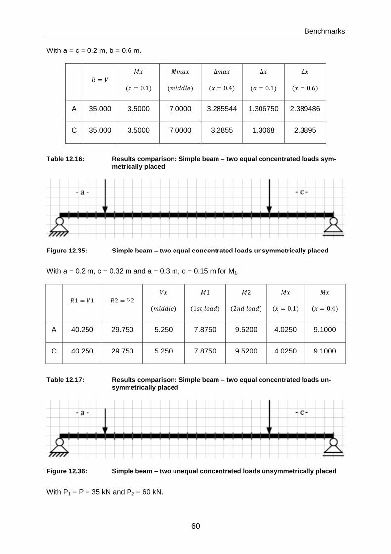
Benchmarks
60
With a = c = 0.2 m, b = 0.6 m.
Ì = . BA
(A = 0.1) B�§A
(�r--��) ∆�§A (A = 0.4)
∆A (§ = 0.1)
∆A (A = 0.6)
A 35.000 3.5000 7.0000 3.285544 1.306750 2.389486
C 35.000 3.5000 7.0000 3.2855 1.3068 2.3895
Table 12.16: Results comparison: Simple beam – two equal concentrated loads sym-metrically placed
Figure 12.35: Simple beam – two equal concentrated loads unsymmetrically placed
With a = 0.2 m, c = 0.32 m and a = 0.3 m, c = 0.15 m for M1.
Ì1 = .1 Ì2 = .2 .A (�r--��)
B1
(1$���§-) B2
(2�-��§-) BA
(A = 0.1) BA
(A = 0.4) A 40.250 29.750 5.250 7.8750 9.5200 4.0250 9.1000
C 40.250 29.750 5.250 7.8750 9.5200 4.0250 9.1000
Table 12.17: Results comparison: Simple beam – two equal concentrated loads un-symmetrically placed
Figure 12.36: Simple beam – two unequal concentrate d loads unsymmetrically placed
With P1 = P = 35 kN and P2 = 60 kN.

Benchmarks
61
Ì1 = .1 Ì2 = .2 .A (�r--��)
B1
(1$���§-) B2
(2�-��§-) BA
(A = 0.1) BA
(A = 0.4) A 50.250 44.750 15.250 10.0500 14.3200 5.0250 13.1000
C 50.250 44.750 15.250 10.050 14.320 5.0250 13.100
Table 12.18: Results comparison: Simple beam – two unequal concentrated loads un-symmetrically placed
12.8 Prestressing
The subsequent formulas are adapted from F. Leonhardt, “Prestressed Concrete. Design
and Construction” and serve to validate the accuracy of this feature of the program. The dif-
ferent tendon layouts are described subsequently.
Tendon Layout
Bea
m E
nd
1 0.20 0.4333 0.5000
2 0.30 0.4333 0.5500
1 0.00 -0.0520 0.2340
2 0.00 0.5720 0.5460
1 0.00 0.0420 -0.1440
2 0.30 -0.0720 -0.0510
1 0.00 -0.1326 0.1287
2 0.00 0.5226 0.4563
1 0.00 0.5850 0.8775
2 0.00 0.5850 0.8775

Benchmarks
62
1 0.40 0.3900 0.3850
2 0.40 0.3900 0.3850
Table 12.19: Analytical results for different tendo n layouts (P = 1)
The input variables according to each system are (f = 0.65 = const.):
A. Eccentricities e1 = 0.2, e2 = 0.3
B. Partition factor ξ = 0.6
C. Partition factor ξ = 0.6 and eccentricities e0 = 0.25, e2 = 0.3
D. Partition factors ξ = 0.6 and β = 0.1
E. Partition factor β =0.1
F. Partition factor β = 0.1 and eccentricity e = 0.4
Tendon Layout
Bea
m E
nd
1 0.20000E+00 0.43333E+00 0.50000E+00
2 0.30000E+00 0.43333E+00 0.55000E+00
1 0.55511E-16 0.52000E-01 0.23400E+00
2 0.00000E+00 -0.57200E+00 0.54600E+00
1 0.13878E-15 0.42000E-01 0.14400E+00
2 0.30000E+00 -0.72000E-01 -0.51000E-01
1 0.27756E-16 -0.13260E+00 0.12870E+00
2 0.17764E-14 0.52260E+00 0.45630E+00
1 0.00000E+00 0.58500E+00 0.87750E+00
2 0.00000E+00 0.58500E+00 0.87750E+00

Benchmarks
63
1 0.40000E+00 0.39000E+00 0.38500E+00
2 0.40000E+00 0.39000E+00 0.38500E+00
Table 12.20: Numerical results for different tendon layouts (P = 1)
12.9 Beam on Elastic Foundation
The simplest possible example is the starting point for the validation of the beam on elastic
foundation and namely without any supports aside from the elastic bedding:
Figure 12.37: Beam on elastic foundation subjected to linear load
For L = 1, E = 30, p = 4, � = � = 15 there is correctly a pure transversal translation of -
0.26667E+00 that is exactly the same as the one calculated with the student version of Info-
CAD Version 13.00a Copyright © InfoGraph GmbH 1995-2013.
For other boundary conditions like a jointed support on one end there is a slight difference: -
0.39960E+00 compared to -0.39967. Due to the lack of knowledge of the implemented pro-
cedure in the commercial code it is not so simple to give an explanation about the source of
this slight variation.
Finishing with the validation of the overall functioning and individual features of the program
with the help of a variety of benchmarks, one can finally test its qualities on a more practical
application.

Application: Railway Bridge with Gerber Joints
64
13 APPLICATION: RAILWAY BRIDGE WITH GERBER JOINTS
The final stage of the validation of the software is conducted by solving a practical problem of
relatively bigger size. This is namely the case study of an existing railway bridge which was a
subject of a loading test. The construction’s characteristics and experimental data were
adapted from the original documentation.
Figure 13.1: Railway bridge with gerber joints
Figure 13.2: Structural model without discretizatio n

Application: Railway Bridge with Gerber Joints
65
From the above shown structural model the right joints at each span (L3, 6, T3) deserve spe-
cial attention in terms of idealization techniques. In reality these gerber joints were construct-
ed with elastomeric pad with certain unknown shear stiffness. At this point a relative axial
displacement is observed which depends on this stiffness as well as on the stiffening effects
of the rail equipment (ballast and rails). The two ultimate choices for these joints are to be
modeled as gerber joints with hinges or with rollers. The reality lies somewhere in-between
these two extremes. Therefore, the third case to study was with a gerber joint connected with
elastic link with a given stiffness which can be calibrated in accordance with the experimental
data in order to improve the results (Biondini, 2014).
Furthermore it is to be clarified that the cross-section is constant only in the middle parts of
the bridge deck in each span and consists of four precast beam SCAC-TAS 130/100 and a
deck. In direction of the columns and the supports this section increases linearly. This vary-
ing cross-section is handled logically with a respectively dense mesh. The input section and
material parameters read as follows:
A I h E
Middle deck 19940 5.540000e+07 420 3.000000e+05
Side deck 105000 5.468750e+08 420 3.000000e+05
Column 4.908739e+04 1.917476e+08 420 3.000000e+05
Table 13.1: Element characteristics of the bridge k ey segments
The loading test was executed with the help of electric train unit with in total 8 axes – 4 in the
middle and 4 on the both ends. This means for the model 8 nodal loads with 4 by 4 equal
amounts. The distance between the axes is known and the train was placed always in the
middle of each span for the three load cases. This is the reason for the denser discretization
in those areas according to the studied load case. The utilized models and the corresponding
structural responses are shown in the following graphics.

Application: Railway Bridge with Gerber Joints
66
Figure 13.3: Discretization for load case 1
Figure 13.4: Structural response to load case 1

Application: Railway Bridge with Gerber Joints
67
Figure 13.5: Discretization for load case 2
Figure 13.6: Structural response to load case 2

Application: Railway Bridge with Gerber Joints
68
Figure 13.7: Discretization for load case 3
Figure 13.8: Structural response to load case 3

Application: Railway Bridge with Gerber Joints
69
Due to the fact that the loading is only symmetrically translated to the centers of the spans
and the first and the third spans are equal it is expected that the displacements resulting from
load cases 1 and 3 should also be symmetrically equal. This, however, is only true for the
numerical solution. In reality the symmetry is never perfect and the displacements were
measured with different instruments in the different spans: 3 levels in the first span, 7 flexi-
meters in the second and 3 theodolites in the third. Positive deflections are downward and in
mm. Consequently follows a graphical analysis of the data.
Load Case 1 2 3
Leve
l
L1 1.32 / /
L2 7.165 -1.335 /
L3 3.495 -3.475 /
Fle
xim
eter
1 -1.03 2.06 /
2 -2.10 4.58 /
3 -1.57 7.56 -0.78
4 -0.98 8.97 -2.05
5 -0.37 8.48 -3.31
6 / 6.28 -4.51
7 / 2.86 -2.22
The
odol
ite
T1 / -2.956 7.856
T2 / / 9.499
T3 / / 1.937
Table 13.2: Experimental data

Application: Railway Bridge with Gerber Joints
70
Figure 13.9: Result comparison: Load case 1 without calibration
Figure 13.10: Result comparison: Load case 1 with c alibration
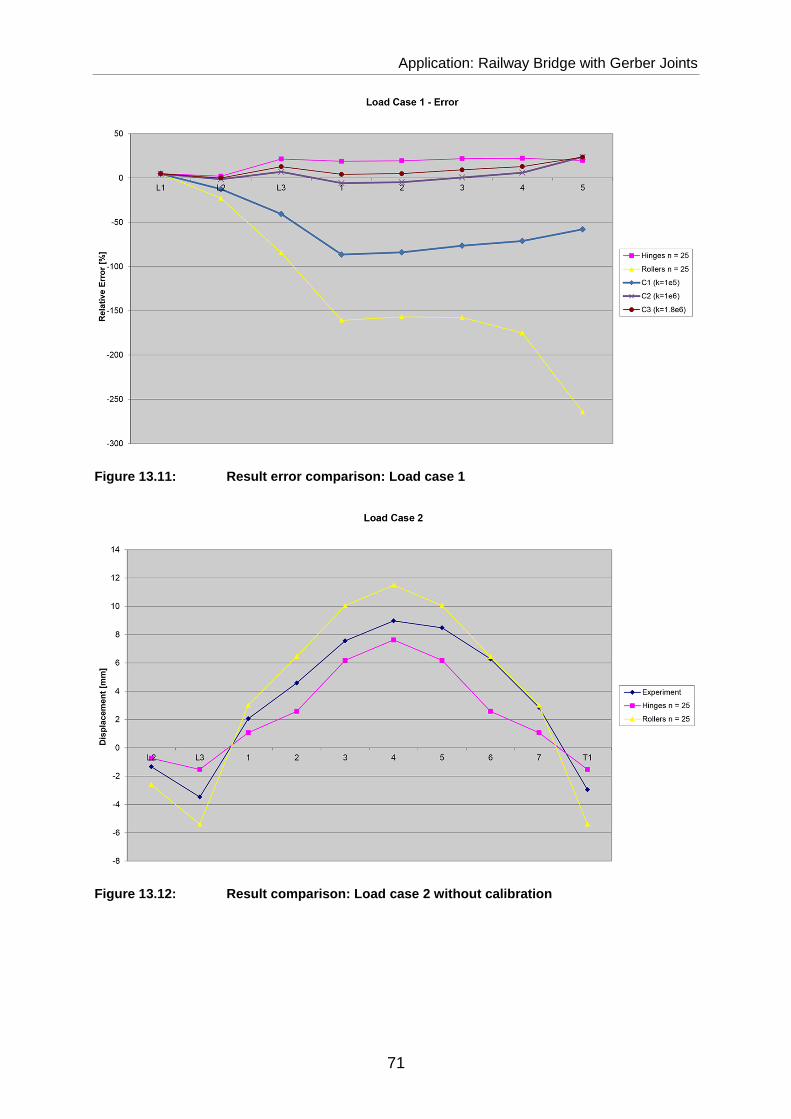
Application: Railway Bridge with Gerber Joints
71
Figure 13.11: Result error comparison: Load case 1
Figure 13.12: Result comparison: Load case 2 withou t calibration
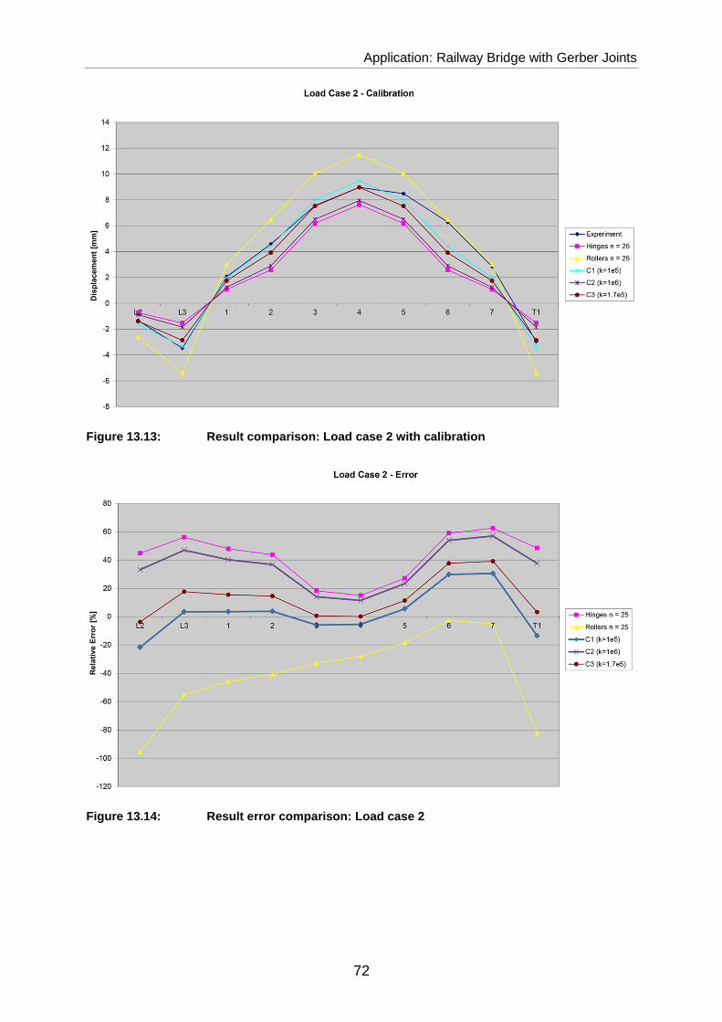
Application: Railway Bridge with Gerber Joints
72
Figure 13.13: Result comparison: Load case 2 with c alibration
Figure 13.14: Result error comparison: Load case 2

Application: Railway Bridge with Gerber Joints
73
Figure 13.15: Result comparison: Load case 3 withou t calibration
Figure 13.16: Result comparison: Load case 3 with c alibration
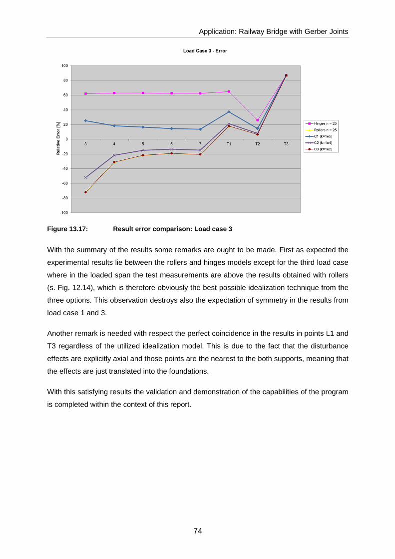
Application: Railway Bridge with Gerber Joints
74
Figure 13.17: Result error comparison: Load case 3
With the summary of the results some remarks are ought to be made. First as expected the
experimental results lie between the rollers and hinges models except for the third load case
where in the loaded span the test measurements are above the results obtained with rollers
(s. Fig. 12.14), which is therefore obviously the best possible idealization technique from the
three options. This observation destroys also the expectation of symmetry in the results from
load case 1 and 3.
Another remark is needed with respect the perfect coincidence in the results in points L1 and
T3 regardless of the utilized idealization model. This is due to the fact that the disturbance
effects are explicitly axial and those points are the nearest to the both supports, meaning that
the effects are just translated into the foundations.
With this satisfying results the validation and demonstration of the capabilities of the program
is completed within the context of this report.

Summary
75
14 SUMMARY
Based on various sources a series of theoretical issues have been discussed within the pro-
ject and utilized practically on a later stage via numerous cross-references during the devel-
opment and evaluating of the computer code. Above all with the help of the lecture notes on
Computational Structural Analysis by Prof. Fabio Biondini it was possible to implement a fully
operating program, enrich with additional features and set perspective for further develop-
ment.
Once it has been shown that with sufficient theoretical background, practical guidance and
motivation a correctly functioning qualitative product can be produced and improved; there is
more understanding about the long process of constantly increasing one program’s capacity.
From keeping in mind the initial structure, through the numerous possible additions to the
need of certain validation it is a challenge to operate with a self-written product.
Furthermore, the overview over the algorithm, functionality, numerical and physical approxi-
mations, tests and other otherwise hidden from the end-user techniques has been immense-
ly enlarged. As already stated potential risks and chances for improvements have been iden-
tified.
Finally, the most beneficial aspect of this work one is able to match the theory with the praxis
in order to create a final useful product. Being a self-made result offers a valuable experi-
ence, new skills, insight and motivation.

References
76
15 REFERENCES
Biondini Fabio, Titi Andrea (2014) Computational Structural Analysis | Lecture Notes: Politecnico di Milano
Cook Robert D., Malkus David S., Plesha Michael E., Witt Robert J. (2002) Concepts and Applications of Finite Element Analysis. Fourth Edition. John Wiley & Sons, Inc.
Corigliano Alberto, Taliercio Alberto (2005) Meccanica computazionale. Soluzione del problema elastico lineare. Bologna: Esculapio
Ghali A., Neville A. M., Brown T. G. (2003) Structural Analysis. A Unified Classical and Matrix Approach. Fifth Edition. New York: Spon Press
Leonhardt F. (1964) Prestressed Concrete. Design and Construction. Berlin-Munich: W. Ernst & Sohn
McGuire William, Gallagher Richard H., Ziemian Ronald D. (2000) Matrix Structural Analysis. Second Edition. New York: John Wiley & Sons, Inc.
Meskouris Konstantin (2010) Baustatik I Vorlesungskript (10/2010): RWTH Aachen University
Press William H., Teukolsky Saul A., Vetterling William T., Flannery Brian P. (1992) Numerical Recipes in FORTRAN. The Art of Scientific Computing. Second Edition. Cambridge: Cambridge University Press
Sacco Riccardo (2013) Numerical Methods for Civil Engineering (December 09, 2013): Politecnico di Milano
Schnepp Johannes (2012) Kontinuumsmechanik I Vorlesungskript: RWTH Aachen University
Will Norbert, Hegger Josef (2012) Massivbau 3 - Spannbeton: RWTH Aachen University

Appendix A: Flowchart of The Code
77
APPENDIX A: FLOWCHART OF THE CODE

Appendix A: Flowchart of The Code
78

Appendix B: User Manual
79
APPENDIX B: USER MANUAL
In the input file which name has to be INPUT.txt the different input sections are respectively
entitled with some clarifications about what the input should be. It is done by putting after
each heading the name of the variable(s) that the program expects behind those brackets
<>. All the variables within these brackets <> is to be written in one line divided by comas or
in other words an opening bracket < indicates the start of a new line. General principle is that
the first line after a heading states the number of the subsequent lines that are going to be
given as an input so that if the number is 0, then the program skips to the next section head-
ing. An exemplar input file is provided:
DEMO INPUT FILE
NODES<NNODES><NODE,X,Y>
5
1,0,0
2,0,4
3,6,4
4,6,4
5,6,0
SECTIONS<NSEC><SEC,A,I,h,Chi>
2
1,0.25,5.208E-3,0.5,1.2
2,0.30,9E-3,0.6,1.2
MATERIALS<NMAT><MAT,E,Nu,Alpha,Gamma>
1
1,30E6,0.2,1.2E-5,25
ELASTIC BEDDING<NSOIL><Ele,bflex,baxis>
1
4,10,10
ELEMENTS<NELE><Ele,Node1,Node2,Sec,Mat,Type>
4
1,1,2,1,1,0
2,2,3,2,1,0
3,4,5,1,1,0
4,1,5,1,1,1
RESTRAINTS<NRES><Node,Direction>
5

Appendix B: User Manual
80
1,1
1,2
1,3
5,1
5,2
LINKS<NLINKS><NMaster,NSlave,Direction>
2
3,4,1
3,4,2
NODAL LOADS<NLOADS><Node,Direction,Force>
1
2,1,50
ELEMENT LOADS<NLOADS><Ele,Px,Py1,Py2,dTtop,dTbot,a/l,Fa>
2
2,0,-25,-25,0,0,0,0
3,0,0,0,10,-10,0,0
PRESTRESSED ELEMENTS<Npres><Ele,NTend><Tend,P,E1,EM,E2>
1
1,2
1,50,0.1,-0.2,0.1
2,100,-0.1,-0.1,-0.1
ELASTIC RESTRAINTS<NERes><Node,Direction,Stiffness>
1
5,3,50000
ELASTIC LINKS<NELinks><Node1,Node2,Direction,Stiffness>
0
IMPOSED DISPLACEMENT<NDisp><Node,Direction,Stiffness>
0
RELATIVE DISPLACEMENT<NRDisp><Node1,Node2,Direction,Stiffness>
0
INCLINED CONSTRAINTS<NICon><Node,Beta,Type,Stiffness/Disp>
0

Appendix B: User Manual
81
The input and especially the output file can be easily modified for the needs of the specific
application. One can for instance restrain themselves from writing down all the displace-
ments or from completely calculating the internal reactions depending on the scale of the
problem and the desired result. In contrary the global stiffness matrix and load vector can be
expressed in the output. Through some modifications it is possible to a-priori define the out-
put fields through the input only for those variables that are of interest. In addition the output
file of this demonstrational input file is listed:
COMPUTATIONAL STRUCTURAL ANALYSIS PROGRAM FRAME
*********************************************************************************************************
DEMO INPUT FILE ********************************************************************************************************* *********************************************************************************************************
READING GEOMETRY
****************
GEOMETRY/SECTIONS/MATERIALS
NUMBER OF NODES = 5
NODE COORDINATE X COORDINATE Y
1 0.000 0.000
2 0.000 4.000
3 6.000 4.000
4 6.000 4.000
5 6.000 0.000
NUMBER OF SECTIONS = 2
SEC AREA INERTHIA DEPTH SHEAR FACTOR
1 0.250 0.521E-02 0.500 1.200
2 0.300 0.900E-02 0.600 1.200

Appendix B: User Manual
82
NUMBER OF MATERIALS = 1
MAT YOUNG POISSON THERMAL COEF WEIGHT
1 0.300E+08 0.200 0.120E-04 0.250E+02
NUMBER OF ELEMENTS ON ELASTIC BEDDING = 1
ELEM FLEXURAL BET AXIAL BETA
4. 0.100E+02 0.100E+02
NUMBER OF ELEMENTS = 4
ELEM NODE 1 NODE 2 SECTION MATERIAL TYPE
1 1 2 1 1 0
2 2 3 2 1 0
3 4 5 1 1 0
4 1 5 1 1 1
*********************************************************************************************************
READING GEOMETRY: DONE *********************************************************************************************************
BOUNDARY CONDITIONS & SYSTEM DOFS
*********************************
NUMBER OF RESTRAINTS = 5
NODE DIRECTION
1 1
1 2
1 3
5 1
5 2
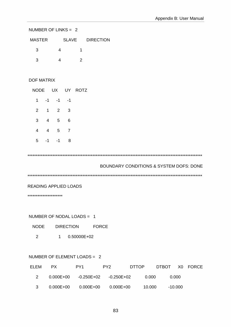
Appendix B: User Manual
83
NUMBER OF LINKS = 2
MASTER SLAVE DIRECTION
3 4 1
3 4 2
DOF MATRIX
NODE UX UY ROTZ
1 -1 -1 -1
2 1 2 3
3 4 5 6
4 4 5 7
5 -1 -1 8
*********************************************************************************************************
BOUNDARY CONDITIONS & SYSTEM DOFS: DONE
*********************************************************************************************************
READING APPLIED LOADS
*********************
NUMBER OF NODAL LOADS = 1
NODE DIRECTION FORCE
2 1 0.50000E+02
NUMBER OF ELEMENT LOADS = 2
ELEM PX PY1 PY2 DTTOP DTBOT X0 FORCE
2 0.000E+00 -0.250E+02 -0.250E+02 0.000 0.000
3 0.000E+00 0.000E+00 0.000E+00 10.000 -10.000

Appendix B: User Manual
84
NUMBER OF PRESTRESSED ELEMENTS = 1
ELEMENT = 1
TENDON P E1 EM E2
1 0.50000E+02 0.100 -0.200 0.100
2 0.10000E+03 -0.100 -0.100 -0.100
EQUIVAL 0.15000E+03 -0.033 -0.133 -0.033
*********************************************************************************************************
READING APPLIED LOADS: DONE *********************************************************************************************************
SYSTEM ASSEMBLY
***************
GLOBAL LOAD VECTOR COMPUTED SUCCESSFULLY
GLOBAL STIFFNESS MATRIX COMPUTED SUCCESSFULLY
*********************************************************************************************************
SYSTEM ASSEMBLY: DONE *********************************************************************************************************
ELASTIC/INCLINED/IMPOSED CONSTRAINTS
************************************
NUMBER OF ELASTIC RESTRAINTS = 1
NODE DIRECTION STIFFNESS
5 3 0.50000E+05
NUMBER OF ELASTIC LINKS = 0
NUMBER OF IMPOSED DISPLACEMENTS = 0
NUMBER OF RELATIVE DISPLACEMENTS = 0
*********************************************************************************************************

Appendix B: User Manual
85
ELASTIC/INCLINED/IMPOSED CONSTRAINTS: DONE *********************************************************************************************************
SOLVING THE SYSTEM
******************
ACCURACY OF THE SOULUTION UP TO 13 DIGITS
APRIORI SYSTEM DATACHECK: DONE
POSSIBLE ILL-CONDITIONING SOURCES: 0
IN-PROGRESS CHECK: DONE
WELL-CONDITIONED SYSTEM
POSTERIORI CHECK: DONE
CONVERGENCE CHECK: DONE
********************************************************************************************************* SOLVING THE SYSTEM: DONE
*********************************************************************************************************
SUMMARY OF THE RESULTS
**********************
NODAL DISPLACEMENTS
NODE UX UY ROTZ
1 0.00000E+00 0.00000E+00 0.00000E+00
2 0.29953E-02 -0.13778E-03 -0.11443E-02
3 0.29752E-02 -0.59549E-04 0.11326E-02
4 0.29752E-02 -0.59549E-04 -0.28748E-03
5 0.00000E+00 0.00000E+00 -0.66165E-03
MAX 0.29953E-02 0.00000E+00 0.11326E-02
MIN 0.00000E+00 -0.13778E-03 -0.11443E-02
*********************************************************************************************************

Appendix B: User Manual
86
FORCES AT END NODES
ELEM N1 T1 M1 N2 T2 M2
1 0.27085E+03 0.48099E+01 0.74317E+02 -0.24585E+03 -0.34810E+02 0.49226E+01
2 0.30190E+02 0.95846E+02 -0.99226E+01 -0.30190E+02 0.99154E+02 0.28422E-13
3 0.99154E+02 0.30190E+02 0.71054E-14 -0.12415E+03 -0.30190E+02 0.12076E+03
4 0.00000E+00 0.15259E+01 -0.15701E+02 0.00000E+00 0.35990E+02 -0.87678E+02
********************************************************************************************************* ********************************************************************************************************* *********************************************************************************************************

Appendix C: Fortran Listing
87
APPENDIX C: FORTRAN LISTING
MODULE GLOBALVAR !DECLARATION OF THE GLOBAL VARIABLES IMPLICIT DOUBLE PRECISION (A-H, O-Z) INTEGER :: NNODE,NDOF,NELE,NSEC,NMAT REAL(2),DIMENSION(:,:),ALLOCATABLE,SAVE :: COORD,CSEC,CMAT,CSOIL INTEGER,DIMENSION(:,:),ALLOCATABLE,SAVE :: IN INTEGER,DIMENSION(:),ALLOCATABLE,SAVE :: ISEC,IMAT,ISOIL !FOR FIRST USE IN THE SUBROUTINE SCODE INTEGER,DIMENSION(:,:),ALLOCATABLE,SAVE :: IDOF !FOR FIRST USE IN THE SUBROUTINE LOADS REAL(2),DIMENSION(:),ALLOCATABLE,SAVE :: VLOADS !GLOBAL LOAD VECTOR REAL(2),DIMENSION(:,:),ALLOCATABLE,SAVE :: ELOADS !LOCAL LOAD VECTOR REAL(2),DIMENSION(:,:),ALLOCATABLE,SAVE :: PRES !PRESTRESSING MATRIX !FOR FIRST USE IN THE SUBROUTINE MKT REAL(2),DIMENSION(6,6) :: ST REAL(2),DIMENSION(6) :: EQFG REAL(2),DIMENSION(:,:),ALLOCATABLE,SAVE :: VK !FOR FIRST USE IN THE SUBROUTINE JOINTS REAL(2),DIMENSION(:),ALLOCATABLE,SAVE :: CINCL !FOR FIRST USE IN THE SUBROUTINE SOLVE REAL(2),DIMENSION(:),ALLOCATABLE,SAVE :: VDISP REAL(2),DIMENSION(:,:),ALLOCATABLE,SAVE :: VKINI END MODULE GLOBALVAR !-----MAIN PROGRAM-------------------------------------------------------------------------------------------------------------- PROGRAM FRAME ! Licensing: ! This code is distributed under the GNU LGPL license. ! ! Modified: ! 21 Juli 2014 ! ! Author: ! FORTRAN90 version by Diyan Rashevski ! ! E-mail: ! [email protected] ! ! Web: ! www.gebor.net USE GLOBALVAR CHARACTER(LEN=80)::TITLE OPEN(9,FILE='MKK.TMP',STATUS='UNKNOWN') OPEN(11,FILE='INPUT.TXT',STATUS='UNKNOWN') OPEN(12,FILE='OUTPUT.TXT',STATUS='UNKNOWN') READ(11,100) TITLE WRITE(12,'(/,A120)') 'COMPUTATIONAL STRUCTURAL ANALYSIS PROGRAM FRAME' CALL STARS WRITE(12,100) TITLE CALL STARS CALL STARS CALL GEOMET CALL STARS CALL SCODE CALL STARS CALL LOADS CALL STARS CALL ASSEMB CALL STARS CALL JOINTS CALL STARS CALL SOLVE CALL STARS CALL STRESS CALL STARS CALL STARS CALL STARS CALL PLOT CLOSE(9)

Appendix C: Fortran Listing
88
CLOSE(11) CLOSE(12) STOP 100 FORMAT(A80) END PROGRAM FRAME !-----GEOMETRY SUBROUTINE------------------------------------------------------------------------------------------------------- SUBROUTINE GEOMET USE GLOBALVAR INTEGER::IDNODE,IDSEC,IDMAT,IDELE,I,J,ICODE CHARACTER(LEN=80)::REC WRITE(12,'(A16,/,A16)') 'READING GEOMETRY','****************' WRITE(12,'(T1,"GEOMETRY/SECTIONS/MATERIALS")') READ(11,100) REC READ(11,*) NNODE ALLOCATE(COORD(NNODE,2)) WRITE(12,'(/,1X,"NUMBER OF NODES =",1X,I3)') NNODE WRITE(12,101)'NODE','COORDINATE X','COORDINATE Y' DO I=1,NNODE READ(11,*) IDNODE,COORD(IDNODE,:) WRITE(12,102) IDNODE,COORD(IDNODE,:) END DO IF (NNODE<2) THEN WRITE(12,'(1X,"ERROR: NUMBER OF NODES <2")') STOP RETURN END IF !READING SECTION PROPERTIES READ(11,*) REC READ(11,*) NSEC ALLOCATE(CSEC(NSEC,4)) WRITE(12,'(/,1X,"NUMBER OF SECTIONS =",1X,I3)') NSEC WRITE(12,103) 'SEC', 'AREA', 'INERTHIA', & & 'DEPTH', 'SHEAR FACTOR' DO I=1,NSEC READ(11,*) IDSEC,CSEC(IDSEC,:) WRITE(12,104) IDSEC,CSEC(IDSEC,:) ICODE=0 DO J=1,3 IF(CSEC(IDSEC,J)<=0) ICODE=J END DO IF(CSEC(IDSEC,4)<0) ICODE=4 IF(ICODE>0) THEN WRITE(12,'(/,1X,"ERROR IN SECTION PROPERTIES - CSEC(",I1,",",I1,")")') IDSEC,ICODE END IF END DO !READING MATERIAL PROPERTIES READ(11,*) REC READ(11,*) NMAT ALLOCATE(CMAT(NMAT,4)) WRITE(12,'(/,1X,"NUMBER OF MATERIALS =",1X,I3)') NMAT WRITE(12,105) 'MAT', 'YOUNG', 'POISSON', & & 'THERMAL COEFF', 'WEIGHT' DO I=1,NMAT READ(11,*) IDMAT,CMAT(IDMAT,:) WRITE(12,106) IDMAT,CMAT(IDMAT,:) ICODE=0 IF(CMAT(IDMAT,1)<=0) ICODE=1 IF(CMAT(IDMAT,2)<=-1) ICODE=2 IF(CMAT(IDMAT,2)>0.5) ICODE=2 IF(CMAT(IDMAT,3)<0) ICODE=3 IF(CMAT(IDMAT,4)<0) ICODE=4 IF(ICODE>0) THEN WRITE(12,'(/,1X,"ERROR IN MATERIAL PROPERTIES - CMAT(",I1,",",I1,")")') IDMAT,ICODE END IF END DO !READING ELASTIC BEDDING PROPERTIES READ(11,*) REC

Appendix C: Fortran Listing
89
READ(11,*) NSOIL ALLOCATE(CSOIL(NSOIL,3)) WRITE(12,'(/,1X,"NUMBER OF ELEMENTS ON ELASTIC BEDDING =",1X,I3)') NSOIL WRITE(12,107) 'ELEM', 'FLEXURAL BETA', 'AXIAL BETA' DO I=1,NSOIL READ(11,*) CSOIL(I,:) WRITE(12,108) CSOIL(I,:) ICODE=0 DO J=1,3 IF(CSOIL(I,J)<=0) ICODE=J END DO IF(ICODE>0) THEN WRITE(12,'(/,1X,"ERROR IN ELASTIC BEDDING - CSOIL(",I1,",",I1,")")') I,ICODE END IF END DO !READING ELEMENT CONNECTIVITIES READ(11,*) REC READ(11,*) NELE ALLOCATE(IN(NELE,2)) ALLOCATE(ISEC(NELE)) ALLOCATE(IMAT(NELE)) ALLOCATE(ISOIL(NELE)) WRITE(12,'(/,1X,"NUMBER OF ELEMENTS =",1X,I3)') NELE WRITE(12,109) 'ELEM', 'NODE 1', 'NODE 2', & & 'SECTION', 'MATERIAL', 'TYPE' DO I=1,NELE READ(11,*) IDELE,(IN(IDELE,J),J=1,2),ISEC(IDELE),& & IMAT(IDELE),ISOIL(NELE) WRITE(12,110) IDELE,(IN(IDELE,J),J=1,2),ISEC(IDELE),& & IMAT(IDELE),ISOIL(NELE) ICODE=0 DO J=1,2 IF(IN(IDELE,J)<=0) ICODE=J END DO IF(ISEC(IDELE)<=0) ICODE=3 IF(IMAT(IDELE)<=0) ICODE=4 IF(ICODE>0) THEN WRITE(12,'(/,1X,"ERROR IN ELEMENT INDICIES - CONNEC(",I1,",",I1,")")') IDSEC,ICODE END IF END DO CALL STARS WRITE(12,'(A120)') 'READING GEOMETRY: DONE' RETURN 100 FORMAT(A80) ! TITLE FORMAT 101 FORMAT(1X,A7,T15,A12,T32,A12) ! NODE LABELS 102 FORMAT(1X,I7,T15,F12.3,T32,F12.3) ! NODE COORDINATES FORMAT 103 FORMAT(1X,A7,T15,A12,T32,A12,T49,A12,T66,A12) ! SECTION LABELS FORMAT 104 FORMAT(1X,I7,T15,F12.3,T32,E12.3,T49,F12.3,T66,F12.3) ! SECTION VALUES FORMAT 105 FORMAT(1X,A7,T15,A12,T32,A12,T49,A12,T66,A12) ! MATERIAL LABELS FORMAT 106 FORMAT(1X,I7,T15,E12.3,T32,F12.3,T49,E12.3,T66,E12.3) ! MATERIAL VALUES FORMAT 107 FORMAT(1X,A7,T15,A12,T32,A12) ! ELASTIC BEDDING LABELS FORMAT 108 FORMAT(1X,F7.0,T15,E12.3,T32,E12.3) ! ELASTIC BEDDING VALUES FORMAT 109 FORMAT(1X,A7,T15,A12,T32,A12,T49,A12,T66,A12,T83,A12) ! ELEMENT LABELS FORMAT 110 FORMAT(1X,I7,T15,I12,T32,I12,T49,I12,T66,I12,T83,I12) ! ELEMENT VALUES FORMAT END SUBROUTINE GEOMET !-----DOFS SUBROUTINE SCODE----------------------------------------------------------------------------------------------------- SUBROUTINE SCODE USE GLOBALVAR INTEGER::I,J,NRES,NLINK,IDNODE,JDIR,NMAST,NSLAVE CHARACTER(LEN=80)::REC ALLOCATE(IDOF(NNODE,3)) IDOF(:,:)=0 !READING THE RESTRAINTS READ(11,*) REC READ(11,*) NRES WRITE(12,'(A33,/,A33)') 'BOUNDARY CONDITIONS & SYSTEM DOFS','*****************************************' WRITE(12,'(/,1X,"NUMBER OF RESTRAINTS =",1X,I3)') NRES WRITE(12,101) 'NODE','DIRECTION' DO I=1,NRES READ(11,*) IDNODE,JDIR WRITE(12,102) IDNODE,JDIR

Appendix C: Fortran Listing
90
IDOF(IDNODE,JDIR)=-1 END DO !READING THE LINKS READ(11,*) REC READ(11,*) NLINK WRITE(12,'(/,1X,"NUMBER OF LINKS =",1X,I3)') NLINK IF (NLINK>0) THEN WRITE(12,103)'MASTER','SLAVE','DIRECTION' DO I=1,NLINK READ(11,*) NMAST,NSLAVE,JDIR WRITE(12,104) NMAST,NSLAVE,JDIR IDOF(NSLAVE,JDIR)=NMAST END DO END IF !MATRIX OF THE DEGREES OF FREEDOM NDOF=0 WRITE(12,'(/,1X,"DOF MATRIX")') WRITE(12,'(4A8)')'NODE','UX','UY','ROTZ' EXT: DO I=1,NNODE INT: DO J=1,3 IF (IDOF(I,J)<0) CYCLE INT IF (IDOF(I,J)==0) THEN NDOF=NDOF+1 IDOF(I,J)=NDOF ELSE IDNODE=IDOF(I,J) IDOF(I,J)=IDOF(IDNODE,J) END IF END DO INT WRITE(12,'(4(4X,I4))') I,(IDOF(I,:)) END DO EXT CALL STARS WRITE(12,'(A120)') 'BOUNDARY CONDITIONS & SYSTEM DOFS: DONE' RETURN 101 FORMAT(1X,A7,T15,A12) ! RESTRAINTS LABELS 102 FORMAT(1X,I7,T15,I12) ! RESTRAINTS VALUES 103 FORMAT(1X,A7,T15,A12,T32,A12) ! LINKS LABELS 104 FORMAT(1X,I7,T15,I12,T32,I12) ! LINKS VALUES END SUBROUTINE SCODE !-----LOADING SUBROUTINE LOADS-------------------------------------------------------------------------------------------------- SUBROUTINE LOADS USE GLOBALVAR INTEGER::I,NNL,IDNODE,JDIR,NEL,IDELE REAL(2)::NFORCE,ELOAD(5),PRE(4) CHARACTER(LEN=80)::REC ALLOCATE(VLOADS(NDOF)) ALLOCATE(ELOADS(NELE,7)) ALLOCATE(PRES(NELE,4)) VLOADS(:)=0. ELOADS(:,:)=0. !READING THE NODAL LOADS READ(11,*) REC READ(11,*) NNL WRITE(12,'(A21,/,A21)') 'READING APPLIED LOADS','*****************************************' WRITE(12,'(/,1X,"NUMBER OF NODAL LOADS =",1X,I3)') NNL IF(NNL>0) THEN WRITE(12,101) 'NODE','DIRECTION','FORCE' DO I=1,NNL READ(11,*) IDNODE,JDIR,NFORCE WRITE(12,102) IDNODE,JDIR,NFORCE JDOF=IDOF(IDNODE,JDIR) VLOADS(JDOF)=VLOADS(JDOF)+NFORCE END DO END IF !READING THE ELEMENT LOADS READ(11,*) REC READ(11,*) NEL WRITE(12,'(/,1X,"NUMBER OF ELEMENT LOADS =",1X,I3)') NEL

Appendix C: Fortran Listing
91
IF(NEL>0) THEN WRITE(12,103) 'ELEM','PX','PY1','PY2','DTTOP','DTBOT','X0','FORCE' DO I=1,NEL READ(11,*) IDELE,ELOAD WRITE(12,104) IDELE,ELOAD ELOADS(IDELE,:)=ELOADS(IDELE,:)+ELOAD END DO END IF !READING PRESTRESSED ELEMENTS READ(11,*) REC READ(11,*) NEP WRITE(12,'(/,1X,"NUMBER OF PRESTRESSED ELEMENTS =",1X,I3)') NEP IF(NEP>0) THEN DO I=1,NEP READ(11,*) IDELE,NTEND FP=0. E1=0. EM=0. E2=0. WRITE(12,'(1X,"ELEMENT =",1X,I3)') IDELE WRITE(12,107) 'TENDON', 'P', 'E1', 'EM', 'E2' DO J=1,NTEND READ(11,*) IDTEND, PRE(1:4) WRITE(12,108) IDTEND, PRE FP=FP + PRE(1) E1=E1 + PRE(1)*PRE(2) EM=EM + PRE(1)*PRE(3) E2=E2 + PRE(1)*PRE(4) END DO PRES(IDELE,1)=FP PRES(IDELE,2)=E1/FP PRES(IDELE,3)=EM/FP PRES(IDELE,4)=E2/FP WRITE(12,109) 'EQUIVALENT', FP, E1/FP, EM/FP, E2/FP END DO END IF CALL STARS WRITE(12,'(A120)') 'READING APPLIED LOADS: DONE' RETURN 101 FORMAT(1X,A7,T15,A12,T32,A12) ! NODAL LOADS LABELS 102 FORMAT(1X,I7,T15,I12,T32,E12.5) ! NODAL LOADS VALUES 103 FORMAT(1X,A7,T15,A12,T32,A12,T49,A12,T66,A12,T83,A12,T100,A12,T117,A12) ! ELEMENT LOADS LABELS 104 FORMAT(1X,I7,T15,E12.3,T32,E12.3,T49,E12.3,T66,F12.3,T83,F12.3,T100,F12.3,T117,F12.3) ! ELEMENT LOADS VALUES 107 FORMAT(1X,A7,T15,A12,T32,A12,T49,A12,T66,A12) ! PRESTRESSING LABELS 108 FORMAT(1X,I7,T15,E12.5,T32,F12.3,T49,F12.3,T66,F12.3) ! PRESTRESSING VALUES 109 FORMAT(1X,A7,T15,E12.5,T32,F12.3,T49,F12.3,T66,F12.3) ! EQUIVALENT TENDON END SUBROUTINE LOADS !-----ELEMENT MATRICES SUBROUTINE MKT------------------------------------------------------------------------------------------- SUBROUTINE MKT(NE) USE GLOBALVAR INTEGER::I,J,N1,N2,ISC,IMT REAL(2)::DX,DY,AL,CA,SA,AA,AJ,AH,CHI,EMOD,& & POISSON,ALPHA,WEIGHT,GMOD,PHI,PX,PY1,PY2,DTBOT,DTTOP,& & TMP(6,6),T(6,6),EQF(6),FP,E1,EM,E2,TETA1,TETA2,CURV,WW,& & X0,FELE,X01 N1=IN(NE,1) N2=IN(NE,2) DX=COORD(N2,1)-COORD(N1,1) DY=COORD(N2,2)-COORD(N1,2) AL=SQRT(DX**2. + DY**2.) CA=DX/AL SA=DY/AL ISC=ISEC(NE) IMT=IMAT(NE) AA=CSEC(ISC,1) AJ=CSEC(ISC,2) AH=CSEC(ISC,3) CHI=CSEC(ISC,4) EMOD=CMAT(IMT,1) POISSON=CMAT(IMT,2)

Appendix C: Fortran Listing
92
ALPHA=CMAT(IMT,3) WEIGHT=CMAT(IMT,4) GMOD=EMOD/(2.*(1.+POISSON)) PHI=12.*CHI*EMOD*AJ/(AL**2.*GMOD*AA) ! DATA FOR CONCENTRATED LOADS WITHING THE ELEMENT X0=ELOADS(NE,6) FELE=ELOADS(NE,7) X0=X0*AL X01=AL - X0 ! STIFFNESS MATRIX COEFFICIENTS ST(:,:)=0. ST(1,1)=EMOD*AA/AL ST(2,2)=12.*EMOD*AJ/((1.+PHI)*AL**3.) ST(3,2)=6.*EMOD*AJ/((1.+PHI)*AL**2.) ST(3,3)=(4.+PHI)*EMOD*AJ/((1.+PHI)*AL) ST(6,3)=(2.-PHI)*EMOD*AJ/((1.+PHI)*AL) ST(4,1)=-ST(1,1) ST(4,4)=ST(1,1) ST(5,2)=-ST(2,2) ST(5,3)=-ST(3,2) ST(5,5)=ST(2,2) ST(6,2)=ST(3,2) ST(6,5)=-ST(3,2) ST(6,6)=ST(3,3) DO I=1,6 DO J=1,6 ST(I,J)=ST(J,I) END DO END DO WRITE(9,*) ST(:,:) ! STORE THE LOCAL STIFFNESS MATRIX IN A SEPARATE FILE ! TRANSFORMATION MATRIX COEFFICIENTS T(:,:)=0. T(1,1)=CA T(1,2)=-SA T(2,1)=SA T(2,2)=CA T(3,3)=1. T(4,4)=CA T(4,5)=-SA T(5,4)=SA T(5,5)=CA T(6,6)=1. WRITE(9,*) T(:,:) ! STORE THE TRANSFORMATION MATRIX TMP=MATMUL(T,ST) ! FORTRAN 90 FUNCTION ST=MATMUL(TMP,TRANSPOSE(T)) ! TRANSFORMATION LOCAL TO GLOBAL REFERENCE SYSTEM EQF(:)=0. PX=ELOADS(NE,1) PY1=ELOADS(NE,2) PY2=ELOADS(NE,3) DTTOP=ELOADS(NE,4) DTBOT=ELOADS(NE,5) PG=WEIGHT*AA PX=PX - PG*SA PY1=PY1 - PG*CA PY2=PY2 - PG*CA QQ=PY2 - PY1 FP=PRES(NE,1) ! PRESTRESSING PART STARTS E1=PRES(NE,2) EM=PRES(NE,3) E2=PRES(NE,4) TETA1=-1./AL*(3.*E1 + E2 - 4.*EM) TETA2=1./AL*(E1 + 3.*E2 - 4.*EM) CURV=4.*(E1 + E2 - 2.*EM)/(AL**2.) WW=FP*CURV PY1=PY1 + WW PY2=PY2 + WW ! PRESTRESSING PART ENDS EQF(1)=EQF(1) + PX*AL/2. EQF(4)=EQF(4) + PX*AL/2. EQF(2)=EQF(2) + PY1*AL/2. EQF(3)=EQF(3) + PY1*AL**2./12. EQF(5)=EQF(5) + PY1*AL/2. EQF(6)=EQF(6) - PY1*AL**2./12. COEF_A=AL/(12.*EMOD*AJ)

Appendix C: Fortran Listing
93
COEF_B=CHI/(AL*AA*GMOD) COEF_C=COEF_B/(COEF_A+COEF_B) EQF(2)=EQF(2) + 9./60.*QQ*AL*(1.+COEF_C/9.) EQF(3)=EQF(3) + 1./30.*QQ*AL**2.*(1.+COEF_C/4.) EQF(5)=EQF(5) + 21./60.*QQ*AL*(1.-COEF_C/21.) EQF(6)=EQF(6) - 1./20.*QQ*AL**2.*(1.-COEF_C/6.) DELTA_TM=(DTTOP+DTBOT)/2. ! CONSTANT PART OF THE THERMAL CONTRIBUTION FH=EMOD*AA*ALPHA*DELTA_TM EQF(1)=EQF(1) - FH EQF(4)=EQF(4) + FH DELTA_TD=(DTTOP-DTBOT)/2. FM=2.*ALPHA*DELTA_TD*EMOD*AJ/AH EQF(3)=EQF(3) + FM EQF(6)=EQF(6) - FM ! CONTRIBUTION OF THE CONCENTRATED LOAD WITHIN THE ELEMENT EQF(2)=EQF(2) + FELE*X0*X01*(X01 - X0)/(AL**3.) + FELE*X01/AL EQF(5)=EQF(5) + FELE*X0*X01*(X0 - X01)/(AL**3.) + FELE*X0/AL EQF(3)=EQF(3) + FELE*X0*(X01**2.)/(AL**2.) EQF(6)=EQF(6) - FELE*X01*(X0**2.)/(AL**2.) WRITE(9,*) EQF(:) ! STORE THE VECTOR OF EQUIVALENT NODAL FORCES EQF(1)=EQF(1) + FP ! CONSIDER THE PRESTRESSING FORCE UNDER SMALL ANGLES ASSUMPTION EQF(2)=EQF(2) + FP*TETA1 EQF(3)=EQF(3) - FP*E1 EQF(4)=EQF(4) - FP EQF(5)=EQF(5) - FP*TETA2 EQF(6)=EQF(6) + FP*E2 EQFG=MATMUL(T,EQF) RETURN END SUBROUTINE MKT !-----ELEMENT MATRICES SUBROUTINE MKW------------------------------------------------------------------------------------------- SUBROUTINE MKW(NE) USE GLOBALVAR INTEGER::I,J,N1,N2,ISC,IMT REAL(2)::DX,DY,AL,CA,SA,AA,AJ,EMOD,& & POISSON,ALPHA,WEIGHT,GMOD,PX,PY1,PY2,& & TMP(6,6),T(6,6),EQF(6),FO(6) N1=IN(NE,1) N2=IN(NE,2) DX=COORD(N2,1)-COORD(N1,1) DY=COORD(N2,2)-COORD(N1,2) AL=SQRT(DX**2. + DY**2.) CA=DX/AL SA=DY/AL ISC=ISEC(NE) IMT=IMAT(NE) AA=CSEC(ISC,1) AJ=CSEC(ISC,2) EMOD=CMAT(IMT,1) POISSON=CMAT(IMT,2) ALPHA=CMAT(IMT,3) WEIGHT=CMAT(IMT,4) GMOD=EMOD/(2.*(1.+POISSON)) DO I=1,SIZE(CSOIL,1) IF(NE==CSOIL(I,1)) THEN BETAAXIS=CSOIL(I,2) BETAFLEX=CSOIL(I,3) AFL=(CSOIL(I,2)/(4.*EMOD*AJ))**(0.25) AAX=SQRT(CSOIL(I,3)/(EMOD*AA)) CYCLE END IF END DO DELTA=SINH(AFL*AL)**2.-SIN(AFL*AL)**2. ST(:,:)=0. ST(1,1)=EMOD*AA*AAX/TANH(AAX*AL) ST(4,1)=EMOD*AA*AAX/SINH(AAX*AL) ST(2,2)=4.*EMOD*AJ*AFL**3.*(SINH(AFL*AL)*COSH(AFL*AL) + SIN(AFL*AL)*COS(AFL*AL))/DELTA ST(3,2)=2.*EMOD*AJ*AFL**2.*(SINH(AFL*AL)*SINH(AFL*AL) + SIN(AFL*AL)*SIN(AFL*AL))/DELTA ST(5,2)=-4.*EMOD*AJ*AFL**3.*(COSH(AFL*AL)*SIN(AFL*AL) + SINH(AFL*AL)*COS(AFL*AL))/DELTA ST(6,2)=2.*EMOD*AJ*AFL**2.*(SINH(AFL*AL)*SIN(AFL*AL) + SINH(AFL*AL)*SIN(AFL*AL))/DELTA ST(3,3)=2.*EMOD*AJ*AFL*(SINH(AFL*AL)*COSH(AFL*AL) - SIN(AFL*AL)*COS(AFL*AL))/DELTA ST(6,3)=2.*EMOD*AJ*AFL*(COSH(AFL*AL)*SIN(AFL*AL) - SINH(AFL*AL)*COS(AFL*AL))/DELTA ST(5,3)=-ST(6,2)

Appendix C: Fortran Listing
94
ST(4,4)=ST(1,1) ST(5,5)=ST(2,2) ST(6,5)=-ST(3,2) ST(6,6)=ST(3,3) DO I=1,6 DO J=1,6 ST(I,J)=ST(J,I) END DO END DO T(:,:)=0. T(1,1)=CA T(1,2)=-SA T(2,1)=SA T(2,2)=CA T(3,3)=1. T(4,4)=CA T(4,5)=-SA T(5,4)=SA T(5,5)=CA T(6,6)=1. EQF(:)=0. PX=ELOADS(NE,1) PY1=ELOADS(NE,2) PY2=ELOADS(NE,3) PG=WEIGHT*AA PX=PX - PG*SA PY1=PY1 - PG*CA PY2=PY2 - PG*CA QQ=PY2 - PY1 FO(:)=0. FO(1)=PX/BETAAXIS FO(2)=PY1/BETAFLEX FO(3)=QQ/(BETAFLEX*AL) FO(4)=PX/BETAAXIS FO(5)=(PY1+QQ)/BETAFLEX FO(6)=QQ/(BETAFLEX*AL) EQF=MATMUL(ST,FO) ! TRANSFORMATION LOCAL TO GLOBAL REFERENCE SYSTEM TMP=MATMUL(T,ST) ST=MATMUL(TMP,TRANSPOSE(T)) EQFG=MATMUL(T,EQF) ! STORING THE ELEMENT MATRICES WRITE(9,*) ST(:,:) ! STORE THE LOCAL STIFFNESS MATRIX IN A SEPARATE FILE WRITE(9,*) T(:,:) ! STORE THE TRANSFORMATION MATRIX WRITE(9,*) EQF(:) ! STORE THE VECTOR OF EQUIVALENT NODAL FORCES RETURN END SUBROUTINE MKW !-----ASSEMBLY SUBROUTINE ASSEMB------------------------------------------------------------------------------------------------ SUBROUTINE ASSEMB USE GLOBALVAR INTEGER::I,J,NCODE(6) ALLOCATE(VK(NDOF,NDOF)) VK(:,:)=0. WRITE(12,'(A15,/,A15)') 'SYSTEM ASSEMBLY','*****************************************' DO NE=1,NELE IF(ISOIL(NE)==0) THEN CALL MKT(NE) ELSE CALL MKW(NE) END IF N1=IN(NE,1) N2=IN(NE,2) NCODE(1:3)=IDOF(N1,:) NCODE(4:6)=IDOF(N2,:) EXT: DO I=1,6 IC=NCODE(I) IF(IC<0) CYCLE EXT VLOADS(IC)=VLOADS(IC) + EQFG(I) INT: DO J=1,6 JC=NCODE(J) IF(JC<0) CYCLE INT VK(IC,JC)=VK(IC,JC) + ST(I,J) END DO INT

Appendix C: Fortran Listing
95
END DO EXT END DO WRITE(12,'(1X,"GLOBAL LOAD VECTOR COMPUTED SUCCESSFULLY")') !WRITE(12,101) 'DOF', 'FORCE' !WRITE(12,102) (I,VLOADS(I),I=1,NDOF) WRITE(12,'(/,1X,"GLOBAL STIFFNESS MATRIX COMPUTED SUCCESSFULLY")') !DO J=1,NDOF ! WRITE(12,'(/,1X,"ROW",10X,"COLUMN",I3)') J ! DO I=1,NDOF ! WRITE(12,102) I,VK(I,J) !! PRINT *,VK(I,J) ! END DO !END DO CALL STARS WRITE(12,'(A120)') 'SYSTEM ASSEMBLY: DONE' RETURN 101 FORMAT(/,1X,A7,T15,A12) 102 FORMAT(1X,I7,T15,E12.5) END SUBROUTINE ASSEMB !-----ELASTIC LINKS SUBROUTINE JOINTS------------------------------------------------------------------------------------------- SUBROUTINE JOINTS USE GLOBALVAR INTEGER::I,J,JDIR INTEGER::NELR,NELL,IDNODE,N1,N2,NTDIS,NRDIS,NINCL REAL(2)::STIFF,ADIS,VKJJ CHARACTER(80)::REC ALLOCATE(CINCL(NNODE)) WRITE(12,'(A36,/,A36)') 'ELASTIC/INCLINED/IMPOSED CONSTRAINTS','*****************************************' !APPLYING ELASTIC RESTRAINTS READ(11,*) REC READ(11,*) NELR WRITE(12,'(1X,"NUMBER OF ELASTIC RESTRAINTS =",1X,I3)') NELR IF(NELR>0) THEN WRITE(12,101) 'NODE', 'DIRECTION', 'STIFFNESS' DO I=1,NELR READ(11,*) IDNODE,JDIR,STIFF WRITE(12,102) IDNODE,JDIR,STIFF JDOF=IDOF(IDNODE,JDIR) VK(JDOF,JDOF)=VK(JDOF,JDOF) + STIFF END DO END IF !APPLYING ELASTIC LINKS READ(11,*) REC READ(11,*) NELL WRITE(12,'(1X,"NUMBER OF ELASTIC LINKS =",1X,I3)') NELL IF(NELL>0) THEN WRITE(12,103) 'NODE1', 'NODE2', 'DIRECTION', 'STIFFNESS' DO I=1,NELL READ(11,*) N1,N2,JDIR,STIFF WRITE(12,104) N1,N2,JDIR,STIFF JDOF1=IDOF(N1,JDIR) JDOF2=IDOF(N2,JDIR) VK(JDOF1,JDOF1)=VK(JDOF1,JDOF1) + STIFF VK(JDOF2,JDOF2)=VK(JDOF2,JDOF2) + STIFF VK(JDOF1,JDOF2)=VK(JDOF1,JDOF2) - STIFF VK(JDOF2,JDOF1)=VK(JDOF2,JDOF1) - STIFF END DO END IF !APPLYING IMPOSED DISPLACEMENTS READ(11,*) REC READ(11,*) NTDIS WRITE(12,'(/,1X,"NUMBER OF IMPOSED DISPLACEMENTS =",1X,I3)') NTDIS IF(NTDIS>0) THEN WRITE(12,105) 'NODE', 'DIRECTION', 'DISPLACEMENT' DO I=1,NTDIS READ(11,*) IDNODE,JDIR,ADIS WRITE(12,106) IDNODE,JDIR,ADIS JDOF=IDOF(IDNODE,JDIR) IF(JDOF==-1) THEN WRITE(12,'(1X,A120)') '---------------------------ERROR: DOF OF IMPOSED DISPLACEMENT MUST
Appendix C: Fortran Listing
96
BE FREE!---' END IF VKJJ=VK(JDOF,JDOF) VK(JDOF,:)=0. VLOADS(:)=VLOADS(:) - VK(:,JDOF)*ADIS VK(:,JDOF)=0. VK(JDOF,JDOF)=VKJJ VLOADS(JDOF)=VKJJ*ADIS END DO END IF !APPLYING RELATIVE DISPLACEMENTS READ(11,*) REC READ(11,*) NRDIS WRITE(12,'(/,1X,"NUMBER OF RELATIVE DISPLACEMENTS =",1X,I3)') NRDIS IF(NRDIS>0) THEN WRITE(12,107) 'NODE1', 'NODE2', 'DIRECTION', 'DISPLACEMENT' DO I=1,NRDIS READ(11,*) N1,N2,JDIR,ADIS WRITE(12,108) N1,N2,JDIR,ADIS JDOF1=IDOF(N1,JDIR) JDOF2=IDOF(N2,JDIR) VKJJ=VK(JDOF1,JDOF1) + VK(JDOF2,JDOF2) DO K=1,NDOF VK(JDOF1,K)=VK(JDOF1,K) + VK(JDOF2,K) END DO VLOADS(JDOF1)=VLOADS(JDOF1) + VLOADS(JDOF2) DO K=1,NDOF VK(JDOF2,K)=0. VK(K,JDOF1)=VK(K,JDOF1) + VK(K,JDOF2) VLOADS(K)=VLOADS(K) - VK(K,JDOF2)*ADIS VK(K,JDOF2)=0. END DO VK(JDOF1,JDOF1)=VK(JDOF1,JDOF1) + VKJJ VK(JDOF1,JDOF2)=-VKJJ VK(JDOF2,JDOF1)=-VKJJ VK(JDOF2,JDOF2)=VKJJ VLOADS(JDOF1)=VLOADS(JDOF1) - VKJJ*ADIS VLOADS(JDOF2)=VKJJ*ADIS END DO END IF !APPLYING INCLINED CONSTRAINTS CINCL(:)=0. ! INITIALIZATION OF INCLINED CONSTRAINTS VECTOR ONE=1. PIGR2=ASIN(ONE) READ(11,*) REC READ(11,*) NINCL IF(NINCL>0) THEN DO NC=1,NINCL READ(11,*) IDNODE,BETA,ITYP,ADIS !ITYP=0 -> ELASTIC RESTRAINTS !ITYP=1 -> IMPOSED DISPLACEMENTS IF(ITYP==0) STIFF=ADIS I=IDOF(IDNODE,1) J=IDOF(IDNODE,2) BETA=BETA*PIGR2/90. CINCL(IDNODE)=BETA SB=SIN(BETA) CB=COS(BETA) ! UPDATE STIFFNESS MATRIX VKII=VK(I,I) VKIJ=VK(I,J) VKJJ=VK(J,J) EXT3:DO NR=1,NDOF IF(NR==I) THEN VK(I,I)=VKII*CB**2. + 2.*VKIJ*SB*CB + VKJJ*SB**2. VK(I,J)=-VKII*SB*CB + VKIJ*(CB**2. - SB**2.) + VKJJ*SB*CB CYCLE EXT3 END IF IF(NR==J) THEN VK(J,I)=-VKII*SB*CB + VKIJ*(CB**2. - SB**2.) + VKJJ*SB*CB VK(J,J)=VKII*SB**2. + 2.*VKIJ*SB*CB + VKJJ*CB**2. CYCLE EXT3 END IF VKRI=VK(NR,I) VKRJ=VK(NR,J)

Appendix C: Fortran Listing
97
VK(NR,I)=VKRI*CB + VKRJ*SB VK(I,NR)=VK(NR,I) VK(NR,J)=-VKRI*SB + VKRJ*CB VK(J,NR)=VK(NR,J) END DO EXT3 ! UPDATE LOAD VECTOR VLI=VLOADS(I) VLJ=VLOADS(J) VLOADS(I)=VLI*CB + VLJ*SB VLOADS(J)=-VLI*SB + VLJ*CB ! APPLICATION OF RESTRAINTS/IMPOSED DISPLACEMENTS IF(ITYP==0) THEN!ELASTIC RESTRAINTS VK(I,I)=VK(I,I) + STIFF ELSE !IMPOSED DISPLACEMENTS VKJJ=VK(I,I) DO K=1,NDOF VK(I,K)=0. VLOADS(K)=VLOADS(K) - VK(K,I)*ADIS VK(K,I)=0. END DO VK(I,I)=VKJJ VLOADS(I)=VKJJ*ADIS END IF END DO END IF CALL STARS WRITE(12,'(A120)') 'ELASTIC/INCLINED/IMPOSED CONSTRAINTS: DONE' RETURN 101 FORMAT(1X,A7,T15,A12,T32,A12) ! ELASTIC RESTRAINTS LABELS 102 FORMAT(1X,I7,T15,I12,T32,E12.5) ! ELASTIC RESTRAINTS VALUES 103 FORMAT(1X,A7,T15,A12,T32,A12,T49,A12) ! ELASTIC LINKS LABELS 104 FORMAT(1X,I7,T15,I12,T32,I12,T49,E12.5) ! ELASTIC LINKS VALUES 105 FORMAT(1X,A7,T15,A12,T32,A12) ! IMPOSED DISPLACEMENTS LABELS 106 FORMAT(1X,I7,T15,I12,T32,F12.5) ! IMPOSED DISPLACEMENTS VALUES 107 FORMAT(1X,A7,T15,A12,T32,A12,T49,A12) ! RELATIVE DISPLACEMENTS LABELS 108 FORMAT(1X,I7,T15,I12,T32,I12,T49,F12.5) ! RELATIVE DISPLACEMENTS VALUES 109 FORMAT(1X,A7,T15,A12,T32,A12,T49,A12) ! INCLINED CONSTRAINTS LABELS 110 FORMAT(1X,I7,T15,F12.5,T32,I12,T49,F12.5) ! INCLINED CONSTRAINTS VALUES END SUBROUTINE JOINTS !-----CONDITIONING CHECK SUBROUTINE DATACHECK----------------------------------------------------------------------------------- SUBROUTINE DATACHECK USE GLOBALVAR IMPLICIT DOUBLE PRECISION (A-H,O-Z) DOUBLE PRECISION KK(NDOF,NDOF),EIGS(NDOF),EIGVECS(NDOF,NDOF),COND,LMAX,LMIN INTEGER :: SMIN KK=VK CALL JACOBI(KK,NDOF,NDOF,EIGS(NDOF),EIGVECS,0) LMAX=0. LMIN=1E16 DO I=1,NDOF EIGS(I)=KK(I,I) IF(LMAX<ABS(EIGS(I))) THEN LMAX=ABS(EIGS(I)) END IF IF(LMIN>ABS(EIGS(I))) THEN LMIN=ABS(EIGS(I)) END IF END DO COND=LMAX/LMIN COND=LOG(COND) WRITE(12,'(1X,"ACCURACY OF THE SOULUTION UP TO ",I2,1X,"DIGITS")') 16-IDNINT(COND) WRITE(12,'(A120)') 'APRIORI SYSTEM DATACHECK: DONE' END SUBROUTINE DATACHECK !-----SUPPORTING SUBROUTINE TO SUBROUTINE DATACHECK------------------------------------------------------------------------------- SUBROUTINE JACOBI(A,N,NP,D,V,NROT) IMPLICIT DOUBLE PRECISION (A-H,O-Z) INTEGER :: N,NP,NROT,NMAX DOUBLE PRECISION A(NP,NP),D(NP),V(NP,NP) PARAMETER (NMAX=500) ! ADOPTED FROM PRESS W., NUMERICAL RECIPES IN FORTRAN) ! COMPUTES ALL EIGENVALUES AND EIGENVECTORS OF A REAL SYMMETRIC MATRIX A, WHICH IS OF SIZE N BY N, STORED IN A PHYSICAL NP BY NP

Appendix C: Fortran Listing
98
! ARRAY. ON OUTPUT, ELEMENTS OF A ABOVE THE DIAGONAL ARE DESTROYED. D RETURNS THE EIGENVALUES OF A IN ITS FIRST N ELEMENTS. V IS ! A MATRIX WITH THE SAME LOGICAL AND PHYSICAL DIMENSIONS AS A, WHOSE COLUMNS CONTAIN, ON OUTPUT, THE NORMALIZED EIGENECTORS OF ! A. NROT RETURNS THE NUMBER OF JACOBI ROTATIONS THAT WERE REQUIRED. INTEGER :: I,IP,IQ,J REAL C,G,H,S,SM,T,TAU,THETA,TRESH,B(NMAX),Z(NMAX) DO IP=1,N ! INITIALIZE THE IDENTITY MATRIX DO IQ=1,N V(IP,IQ)=0. END DO V(IP,IP)=1. END DO DO IP=1,N B(IP)=A(IP,IP) ! INITIALIZE B AND D TO THE DIAGONAL OF A D(IP)=B(IP) Z(IP)=0 END DO NROT=0 DO I=1,50 SM=0. DO IP=1,N-1 ! SUM OFF-DIAGONAL ELEMENTS DO IQ=IP+1,N SM=SM + ABS(A(IP,IQ)) END DO END DO IF(SM.EQ.0.) RETURN ! THE NORMAL RETURN, WHICH RELIES ON QUADRATIC CONVERGENCE TO MACHINE UNDERFLOW IF(I.LT.4) THEN TRESH=0.2*SM/N**2 ! ...ON THE FIRST THREE SWEEPS ELSE TRESH=0. ! ...THEREAFTER END IF DO IP=1,N-1 DO IQ=IP+1,N G=100.*ABS(A(IP,IQ)) ! AFTER FOUR SWEEPS, SKIP THE ROTATION IF THE OFF-DIAGONAL ELEMENT IS SMALL IF((I.GT.4).AND.(ABS(D(IP))+G.EQ.ABS(D(IP))).AND.(ABS(D(IQ))+G.EQ.ABS(D(IQ)))) THEN A(IP,IQ)=0. ELSE IF(ABS(A(IP,IQ)).GT.TRESH) THEN H=D(IQ) - D(IP) IF(ABS(H)+G.EQ.ABS(H)) THEN T=A(IP,IQ)/H ! T=1/(2THETA) ELSE THETA=0.5*H/A(IP,IQ) T=1./(ABS(THETA)+SQRT(1.+THETA**2.)) IF(THETA.LT.0.) T=-T END IF C=1./SQRT(1 + T**2.) S=T*C TAU=S/(1. + C) H=T*A(IP,IQ) Z(IP)=Z(IP) - H Z(IQ)=Z(IQ) + H D(IP)=D(IP) - H D(IQ)=D(IQ) + H A(IP,IQ)=0. DO J=1,IP-1 ! CASE OF ROTATIONS 1<=J<P G=A(J,IP) H=A(J,IQ) A(J,IP)=G - S*(H + G*TAU) A(J,IQ)=H + S*(G - H*TAU) END DO DO J=IP+1,IQ-1 ! CASE OF ROTATIONS P<J<Q G=A(IP,J) H=A(J,IQ) A(IP,J)=G - S*(H + G*TAU) A(J,IQ)=H + S*(G - H*TAU) END DO DO J=IQ+1,N ! CASE OF ROTATIONS Q<J<=N G=A(IP,J) H=A(IQ,J) A(IP,J)=G - S*(H + G*TAU) A(IQ,J)=G + S*(G - H*TAU) END DO DO J=1,N

Appendix C: Fortran Listing
99
G=V(J,IP) H=V(J,IQ) V(J,IP)=G - S*(H + G*TAU) V(J,IQ)=H + S*(G - H*TAU) END DO NROT=NROT + 1 END IF END DO END DO DO IP=1,N B(IP)=B(IP) + Z(IP) D(IP)=B(IP) ! UPDATE D WITH THE SUM OF TAPQ AND REINITIALIZE Z Z(IP)=0. END DO END DO PAUSE 'TOO MANY ITERATIONS IN JACOBI' RETURN END SUBROUTINE JACOBI !-----SOLVE SUBROUTINE SOLVE---------------------------------------------------------------------------------------------------- SUBROUTINE SOLVE USE GLOBALVAR INTEGER::I,J,K,DOF,DEC REAL(2)::DNOD(3),DMX(3),DMN(3),PVAL REAL(2),DIMENSION(:),ALLOCATABLE::TEST ALLOCATE(VDISP(NDOF)) ALLOCATE(TEST(NDOF)) ALLOCATE(VKINI(NDOF,NDOF)) WRITE(12,'(A18,/,A18)') 'SOLVING THE SYSTEM','*****************************************' CALL DATACHECK !INITIALIZATION OF THE VECTOR OF THE CONSTANT TERMS !LOAD VECTOR -> DISPLACEMENT VECTOR VDISP=VLOADS VKINI=VK !GAUSSIAN ELIMINATION METHOD + DIAGONAL DECAY ERROR TEST DO I=1,NDOF TEST(I)=VK(I,I) END DO DEC=0 DO I=1,NDOF DO K=I+1,NDOF VK(I,K)=VK(I,K)/VK(I,I) END DO VDISP(I)=VDISP(I)/VK(I,I) IF(TEST(I)/VK(I,I)>=1E10) THEN DEC=DEC+100 ELSE IF(TEST(I)/VK(I,I)>=1E3) THEN DEC=DEC+1 END IF VK(I,I)=1. DO J=I+1,NDOF DO K=I+1,NDOF VK(J,K)=VK(J,K) - VK(J,I)*VK(I,K) END DO VDISP(J)=VDISP(J) - VK(J,I)*VDISP(I) VK(J,I)=0. END DO END DO !DIAGONAL DECAY ERROR TEST RESULTS IF(DEC>=100) THEN WRITE(12,'(A29,/,A29,/,A29)') '******************WARNING!***','THE SYSTEM IS ILL-CONDITIONED','-------------------------------' ELSE WRITE(12,'(1X,A34,1X,I5)') 'POSSIBLE ILL-CONDITIONING SOURCES:',DEC END IF !BACKWARD SUBSTITUTION DO I=NDOF,1,-1 DO K=I+1,NDOF VDISP(I)=VDISP(I) - VK(I,K)*VDISP(K) END DO END DO WRITE(12,'(A120)') 'IN-PROGRESS CHECK: DONE' ! POSTERIORI ERROR TEST VIA WORK OF RESIDUALS CALL POSTERIORI CALL STARS WRITE(12,'(A120)') 'SOLVING THE SYSTEM: DONE'

Appendix C: Fortran Listing
100
CALL STARS ! SUMMARY OF THE DISPLACEMENTS WRITE(12,'(A22,/,A22)') 'SUMMARY OF THE RESULTS','*****************************************' WRITE(12,'(/,1X,"NODAL DISPLACEMENTS")') WRITE(12,102) 'NODE','UX','UY','ROTZ' DNOD=0. DMX=-1.E6 DMN=1.E6 EXT:DO ND=1,NNODE ! ROTATE INCLINED DISPLACEMENTS BACK TO THE GLOBAL REFERENCE SYSTEM BETA=CINCL(ND) IF(BETA==0.) CYCLE EXT I=IDOF(ND,1) J=IDOF(ND,2) SB=SIN(BETA) CB=COS(BETA) VDI=VDISP(I) VDJ=VDISP(J) VDISP(I)=VDI*CB - VDJ*SB VDISP(J)=VDI*SB + VDJ*CB END DO EXT DO I=1,NNODE DO J=1,3 IF(IDOF(I,J)<0) THEN DNOD(J)=0. ELSE DOF=IDOF(I,J) DNOD(J)=VDISP(DOF) END IF PVAL=DMX(J) DMX(J)=MAX(DNOD(J),PVAL) PVAL=DMN(J) DMN(J)=MIN(DNOD(J),PVAL) END DO WRITE(12,103) I,(DNOD(J),J=1,3) END DO WRITE(12,'(/)') WRITE(12,104) 'MAX', (DMX(J),J=1,3) WRITE(12,104) 'MIN', (DMN(J),J=1,3) RETURN 102 FORMAT(1X,A7,T15,A12,T32,A12,T49,A12) ! NODE DISPLACEMENTS LABELS 103 FORMAT(1X,I7,T15,E12.5,T32,E12.5,T49,E12.5) ! NODE DISPLACEMENTS VALUES 104 FORMAT(1X,A7,T15,E12.5,T32,E12.5,T49,E12.5) ! MAX/MIN VALUES END SUBROUTINE SOLVE !-----WORK OF RESIDUALS TEST SUBROUTINE POSTERIORI---------------------------------------------------------------------------------------- SUBROUTINE POSTERIORI USE GLOBALVAR REAL::WORK REAL(2),DIMENSION(:),ALLOCATABLE::DELTAVLOADS ALLOCATE(DELTAVLOADS(NDOF)) WORK=0.5*DOT_PRODUCT(VLOADS,VDISP) DELTAVLOADS=MATMUL(VKINI,VDISP) - VLOADS DELTAWORK=0.5*DOT_PRODUCT(DELTAVLOADS,VDISP) ERRORW=DELTAWORK/WORK IF(ERRORW>=1E-2) THEN WRITE(12,'(A29,/,A29,/,A29)') '****************WARNING!***','POSSIBLY ILL-CONDITIONED SYSTEM','-------------------------------' ELSE IF(ERRORW<=1E-5) THEN WRITE(12,'(1X,A34)') 'WELL-CONDITIONED SYSTEM' END IF WRITE(12,'(A120)') 'POSTERIORI CHECK: DONE' DELTAF=SQRT(DOT_PRODUCT(DELTAVLOADS,DELTAVLOADS)) FF=SQRT(DOT_PRODUCT(VLOADS,VLOADS)) ERRORF=DELTAF/FF IF(ERRORF<=1E-3) THEN IF(ERRORW<=1E-3) THEN WRITE(12,'(A120)') 'CONVERGENCE CHECK: DONE' END IF ELSE IF(ERRORW>1E-3) THEN WRITE(12,'(A120)') 'CONVERGENCE CHECK: FAIL' END IF

Appendix C: Fortran Listing
101
RETURN END SUBROUTINE POSTERIORI !-----INTERNAL ACTIONS SUBROUTINE STRESS---------------------------------------------------------------------------------------- SUBROUTINE STRESS USE GLOBALVAR INTEGER::I,J,NCODE(6) REAL(2)::QS(6),QSL(6),T(6,6),EQF(6),QF(6) REWIND(9) WRITE(12,'(/,1X,"FORCES AT END NODES")') WRITE(12,100) 'ELEM', 'N1', 'T1', 'M1', 'N2', 'T2', 'M2' DO NE=1,NELE N1=IN(NE,1) N2=IN(NE,2) NCODE(1:3)=IDOF(N1,:) NCODE(4:6)=IDOF(N2,:) READ(9,*) ST READ(9,*) T READ(9,*) EQF DO I=1,6 JDOF=NCODE(I) IF(JDOF<0) THEN QS(I)=0 ELSE QS(I)=VDISP(JDOF) END IF END DO QSL=MATMUL(TRANSPOSE(T),QS) DO I=1,6 QF(I)=-EQF(I) DO J=1,6 QF(I)=QF(I) + ST(I,J)*QSL(J) END DO END DO WRITE(12,101) NE,(QF(I),I=1,6) END DO RETURN 100 FORMAT(1X,A7,T15,A12,T32,A12,T49,A12,T66,A12,T83,A12,T100,A12) 101 FORMAT(1X,I7,T15,E12.5,T32,E12.5,T49,E12.5,T66,E12.5,T83,E12.5,T100,E12.5) END SUBROUTINE STRESS !-----OUTPUT SUBROUTINE PLOT---------------------------------------------------------------------------------------------------- SUBROUTINE PLOT USE GLOBALVAR IMPLICIT DOUBLE PRECISION (A-H,O-Z) INTEGER::I,J,NCODE(6) REAL(2)::QS(6),QSL(6),T(6,6),EQF(6),QF(6) REWIND(9) ! REWIND THE TEMPORARY FILE OPEN(33,FILE='PLOT.DAT',STATUS='UNKNOWN') ! OPEN FILE 33 (INPUT DATA FOR PLOT.EXE) !WRITE THE COORDINATES AND INCIDENCE WRITE(33,*) NNODE,NELE DO I=1,NNODE WRITE(33,*) (COORD(I,J),J=1,2) END DO DO NE=1,NELE WRITE(33,*) (IN(NE,J),J=1,2) END DO ! WRITING THE POSITION OF THE CONCENTRATED LOADS WITHIN THE ELEMENT DO NE=1,NELE WRITE(33,*) ELOADS(NE,6) END DO DO NE=1,NELE ! LOOP OVER ALL ELEMENTS N1=IN(NE,1) N2=IN(NE,2) NCODE(1:3)=IDOF(N1,1:3) NCODE(4:6)=IDOF(N2,1:3) READ(9,*) ST READ(9,*) T READ(9,*) EQF DO I=1,6 ! NODAL DISPLACEMENTS IN THE GLOBAL REFERENCE SYSTEM JDOF=NCODE(I)

Appendix C: Fortran Listing
102
IF(JDOF==-1) THEN QS(I)=0. ELSE !PRINT*,JDOF QS(I)=VDISP(JDOF) ENDIF END DO QSL=MATMUL(TRANSPOSE(T),QS) ! NODAL DISPLACEMENTS IN THE LOCAL REFERENCE SYSTEM DO I=1,6 ! FORCES AT END NODES QF(I)=-EQF(I) DO J=1,6 QF(I)=QF(I) + ST(I,J)*QSL(J) END DO END DO DX=COORD(N2,1) - COORD(N1,1) ! DISPLACEMENTS AND FORCES ALONG THE LENGTH OF THE ELEMENT DY=COORD(N2,2) - COORD(N1,2) AL=SQRT(DX**2. + DY**2.) CA=DX/AL SA=DY/AL ISC=ISEC(NE) IMT=IMAT(NE) AA=CSEC(ISC,1) WEIGHT=CMAT(IMT,4) PX=ELOADS(NE,1) PY1=ELOADS(NE,2) PY2=ELOADS(NE,3) FP=PRES(NE,1) E1=PRES(NE,2) EM=PRES(NE,3) E2=PRES(NE,4) CURV=4.*(E1 + E2 - 2.*EM)/(AL**2.) WW=FP*CURV PY1=PY1 + WW PY2=PY2 + WW X0=ELOADS(NE,6) AL0=X0*AL FELE=ELOADS(NE,7) IF(X0==0.) THEN DO I=0,20 XX=AL*DBLE(I)/20. PY=PY1 + (PY2 - PY1)*XX/2. UU=U(QSL,XX,AL) VV=V(QSL,XX,AL) SSN=-QF(1) - PX*XX SST=QF(2) + (PY1 + PY)*XX/2. SSM=-QF(3) + QF(2)*XX + PY1*XX**2./2. + (PY - PY1)*XX**2./6. WRITE(33,*) UU,VV,SSN,SST,SSM END DO ELSE DO K=1,2 IF(K==1) THEN AL=X0*AL DO I=0,20 XX=AL1*DBLE(I)/20. PY=PY1 + (PY2 - PY1)*XX/AL UU=U(QSL,XX,AL) VV=V(QSL,XX,AL) SSN=-QF(1) - PX*XX SST=QF(2) + (PY1 + PY)*XX/2. SSM=-QF(3) + QF(2)*XX + PY1*XX**2./2. + (PY1 - PY1)*XX**2./6. WRITE(33,*) UU,VV,SSN,SST,SSM END DO ELSE AL2=(1. - X0)*AL FORCE=FELE DO I=0,20 XX=AL0 + AL2*DBLE(I)/20. PY=PY1 + (PY2 - PY1)*XX/AL UU=U(QSL,XX,AL) VV=V(QSL,XX,AL) SSN=-QF(1) - PX*XX SST=QF(2) + (PY1 + PY)*XX/2. + FORCE SSM=-QF(3) + QF(2)*XX + PY1*XX**2./2. & & + (PY - PY1)*XX**2./6. + FORCE*(XX - AL0) WRITE(33,*) UU,VV,SSN,SST,SSM END DO END IF

Appendix C: Fortran Listing
103
END DO END IF END DO CLOSE(33) RETURN END SUBROUTINE PLOT !-----SUPPORTING FUNCTIONS TO SUBROUTINE PLOT----------------------------------------------------------------------------------- DOUBLE PRECISION FUNCTION F(I,AL,X) IMPLICIT DOUBLE PRECISION (A-H,O-Z) CSI=X/AL SELECT CASE(I) CASE(1) F=1.-CSI CASE(4) F=CSI CASE(2) F=1. - 3.*CSI**2. + 2.*CSI**3. CASE(3) F=AL*(CSI - 2.*CSI**2. + CSI**3.) CASE(5) F=3.*CSI**2. - 2.*CSI**3. CASE(6) F=AL*(CSI**3. - CSI**2.) END SELECT END FUNCTION F DOUBLE PRECISION FUNCTION U(QSL,X,AL) IMPLICIT DOUBLE PRECISION (A-H,O-Z) DIMENSION::QSL(6) U=0. DO I=1,4,3 U=U + F(I,AL,X)*QSL(I) END DO RETURN END FUNCTION U DOUBLE PRECISION FUNCTION V(QSL,X,AL) IMPLICIT DOUBLE PRECISION (A-H,O-Z) DIMENSION::QSL(6) V=0. DO I=2,3 V=V + F(I,AL,X)*QSL(I) END DO DO I=5,6 V=V + F(I,AL,X)*QSL(I) END DO RETURN END FUNCTION V !-----FORMAT SUBROUTINE STARS--------------------------------------------------------------------------------------------------- SUBROUTINE STARS WRITE(12,'(A120)') '***********************************************************************************************************' RETURN END SUBROUTINE STARS

Declaration
104
DECLARATION
Hereby I declare that I have completed this report independently. I have used only the explic-
itly named literature references and sources. Literally or identically formulated statements
that were adopted from a specific source have been identified as such.
Milano, den 25.07.2014
Diyan Rashevski
Signature