computational quantum mechanics (b) computational quantum...
TRANSCRIPT
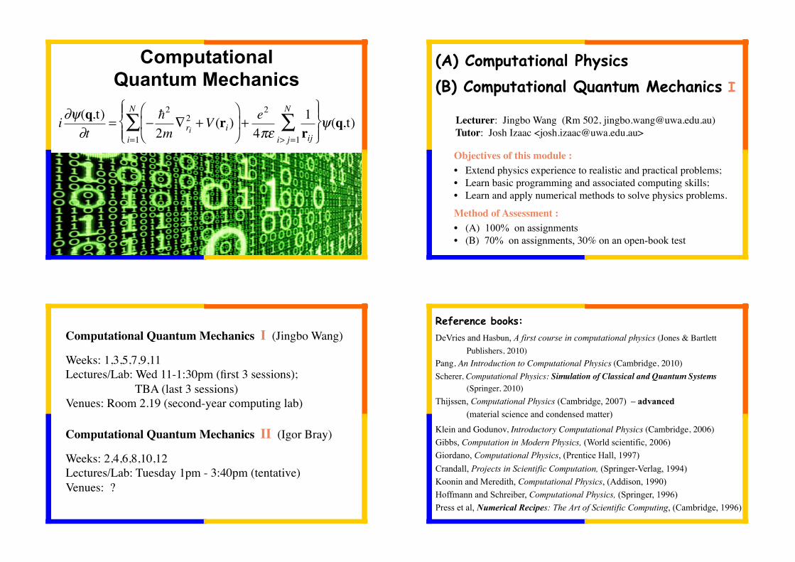
Computational Quantum Mechanics
�
i∂ψ(q,t)
∂t= −
2
2m∇ ri
2+V (ri)
⎛
⎝
⎜
⎞
⎠
⎟
i=1
N
∑ +e2
4πε1
riji> j=1
N
∑⎧
⎨ ⎪
⎩ ⎪
⎫
⎬ ⎪
⎭ ⎪ ψ(q,t)
! ! Lecturer: Jingbo Wang (Rm 502, [email protected])! Tutor: Josh Izaac <[email protected]>!
(A) Computational Physics (B) Computational Quantum Mechanics
Objectives of this module : !!
• Extend physics experience to realistic and practical problems; !• Learn basic programming and associated computing skills; !• Learn and apply numerical methods to solve physics problems.
Method of Assessment : !!
• (A) 100% on assignments!• (B) 70% on assignments, 30% on an open-book test
I!
Computational Quantum Mechanics I (Jingbo Wang)!!
Weeks: 1,3,5,7,9,11!Lectures/Lab: Wed 11-1:30pm (first 3 sessions); ! TBA (last 3 sessions)!Venues: Room 2.19 (second-year computing lab) !!Computational Quantum Mechanics II (Igor Bray)!!
Weeks: 2,4,6,8,10,12!Lectures/Lab: Tuesday 1pm - 3:40pm (tentative)!Venues: ?!
Reference books:
DeVries and Hasbun, A first course in computational physics (Jones & Bartlett !Publishers, 2010) !
Pang, An Introduction to Computational Physics (Cambridge, 2010)!Scherer, Computational Physics: Simulation of Classical and Quantum Systems
!(Springer, 2010)!Thijssen, Computational Physics (Cambridge, 2007) – advanced
(material science and condensed matter)
Klein and Godunov, Introductory Computational Physics (Cambridge, 2006)!Gibbs, Computation in Modern Physics, (World scientific, 2006)
Giordano, Computational Physics, (Prentice Hall, 1997) Crandall, Projects in Scientific Computation, (Springer-Verlag, 1994) Koonin and Meredith, Computational Physics, (Addison, 1990) Hoffmann and Schreiber, Computational Physics, (Springer, 1996) Press et al, Numerical Recipes: The Art of Scientific Computing, (Cambridge, 1996)
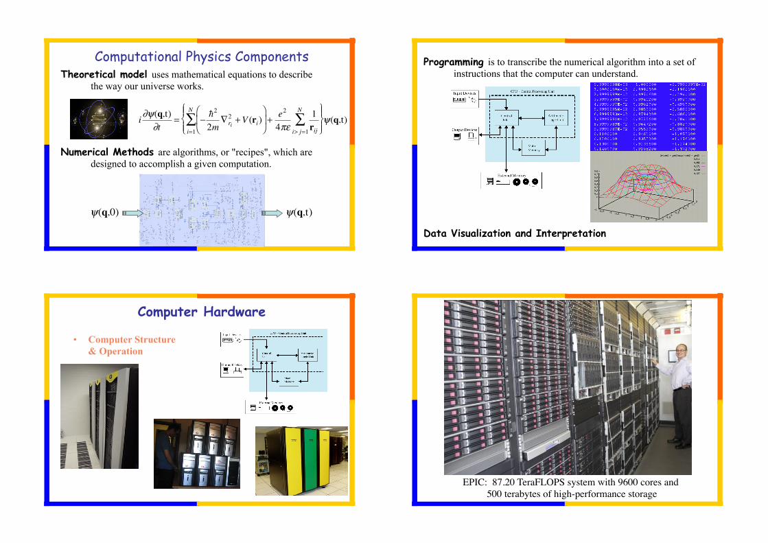
Theoretical model uses mathematical equations to describe the way our universe works.
Numerical Methods are algorithms, or "recipes", which are designed to accomplish a given computation.
Computational Physics Components
�
i∂ψ(q,t)
∂t= −
2
2m∇ ri
2+V (ri)
⎛
⎝
⎜
⎞
⎠
⎟
i=1
N
∑ +e2
4πε1
riji> j=1
N
∑⎧
⎨ ⎪
⎩ ⎪
⎫
⎬ ⎪
⎭ ⎪ ψ(q,t)
�
ψ(q,0)
�
ψ(q,t)
Programming is to transcribe the numerical algorithm into a set of instructions that the computer can understand.
Data Visualization and Interpretation
Computer Hardware
• Computer Structure & Operation
EPIC: 87.20 TeraFLOPS system with 9600 cores and !500 terabytes of high-performance storage!

FORNAX: 1152 Intel Xeon X5650 CPUs, 96 NVIDIA Tesla C2075 GPU, 4.6 TB RAM, and 500TB of high-performance storage! iVEC’s StorageTek stores up to 32.5 PB of data!
Computer Software (a series of instructions to the CPU)
Minimum software components :!
2. Editor • PCs & Macs : WORD, BBEdit, SimpleText, etc !!• Workstations and supercomputers : gvim, xemacs, gedit, nano!
3. Compiler!• programming languages:
Basic, Pascal, Fortran, C, C++, Java, Python
• software packages: Matlab, Maple, Mathematica !!
1. Operating system!• PCs & Macs : DOS, Windows, MacOS, UNIX • workstations and supercomputers : UNIX !!

http://internal.physics.uwa.edu.au/~wang/CQM/FortranFacesFuture.pdf� http://internal.physics.uwa.edu.au/~wang/CQM/FortranFacesFuture.pdf�
Why Fortran?
• Fortran was developed for FORmula TRANslation, and it is very good at that.
• Fortran is designed to help develop codes quickly and easily, hiding some of the complications of other languages (eg. C and Java).
• The maturity of optimising compilers provides such a performance benefit that other languages cannot yet compete.
• Many physics computer programs, are written in Fortran (see, e.g. http://www.cpc.cs.qub.ac.uk/cpc).
file://localhost/Users/iMacIntel/WRITE/LectureNotes/ComputationalPhysics/CQM2012/CPC_Fortran.html!
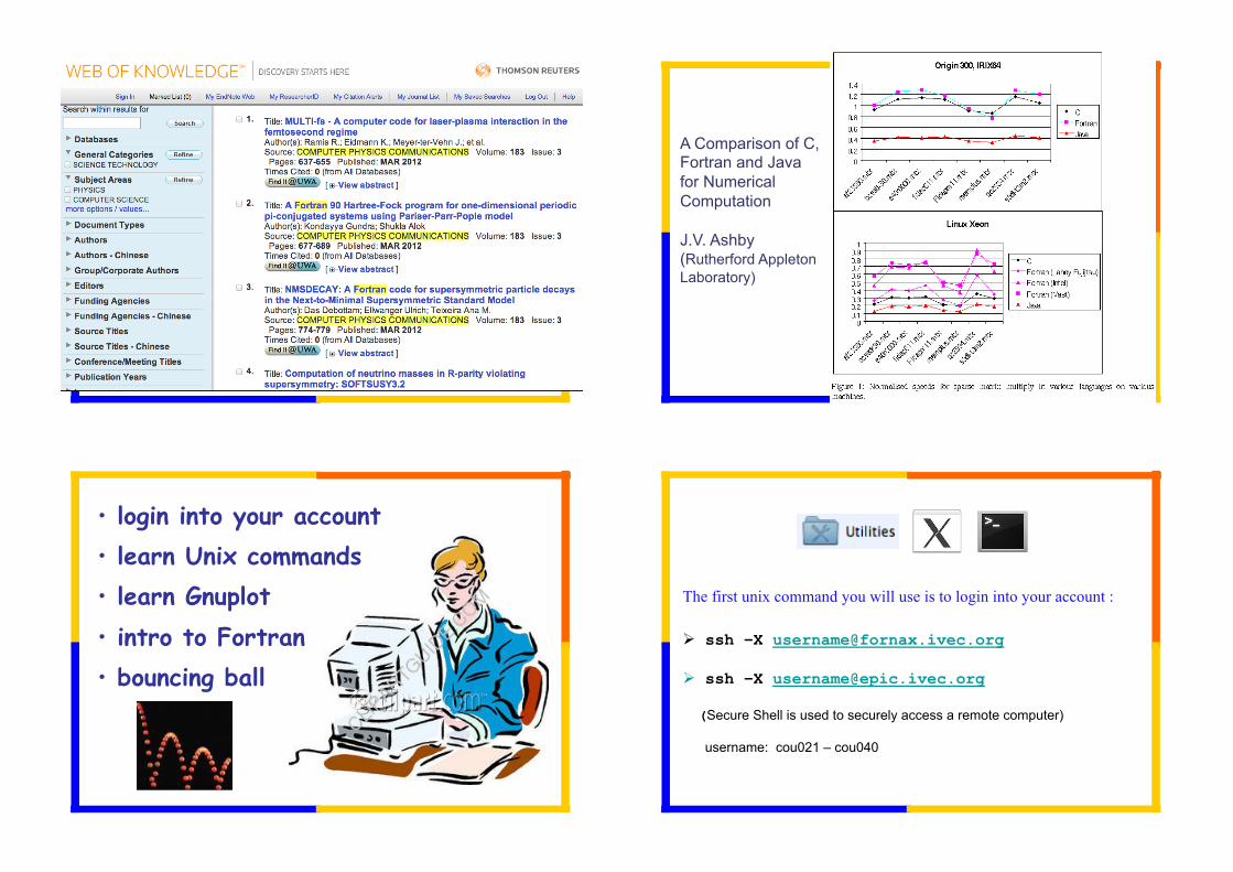
A Comparison of C, Fortran and Java for Numerical Computation J.V. Ashby (Rutherford Appleton Laboratory)
• login into your account • learn Unix commands • learn Gnuplot • intro to Fortran • bouncing ball
The first unix command you will use is to login into your account :
!! ssh –X [email protected]
! ssh –X [email protected]! (Secure Shell is used to securely access a remote computer) username: cou021 – cou040

File system and home directory
!
Introduction to UNIX Second unix command ! passwd changes your password (make sure you remember!) Then ! mkdir <directory> creates a directory
ls lists the files of the current directory cd <directory> change directory pwd shows present working directory cp <file1> <file2> copies file1 to file2
(e.g. cp ~jwang1/cp/bounce.dat b.dat) mv <file1> <file2> change filenames rm <file> removes a file mkdir <directory> creates a directory rmdir <directory> removes a directory man <command> online manual man –k <keyword> search for the specified string in *all* man pages. vi <filename> a sophisticated text editor nano or pico or jpico <filename> more novice friendly text editors more <filename> display a file a page at a time tail <filename> display a file a page at a time grep <word> <filename> searches files for specified words logout exit
Basic commands (http://internal.physics.uwa.edu.au/~wang/unixtut/)!
GNUPLOT is a free, command-driven, interactive, function and data plotting program. Gnuplot can be run under DOS, Windows, Macintosh OS, VMS, Linux, and many others.
Data Visualization
! gnuplot gnuplot> plot sin(x)
gnuplot> splot sin(x)*cos(y)
gnuplot> plot sin(x) title 'Sine', tan(x) title 'Tangent’
gnuplot> plot "force.dat" using 1:2
gnuplot> plot "force.dat" using 1:2 title 'data A', \ "force.dat" using 1:3 title 'data B’
gnuplot> help plot using
gnuplot> set yrange [20:500]
gnuplot> plot "force.dat" using 1:2 title 'data A’ with lines, \ "force.dat" using 1:3 title 'data B’ w linespoints
gnuplot> exit
Gnuplot ( http://internal.physics.uwa.edu.au/~wang/Gnu/GnuplotSummary.pdf, !! http://internal.physics.uwa.edu.au/~wang/Gnu/GnuplotTutorial.pdf )!
cp ~jwang1/cp/force.dat .!
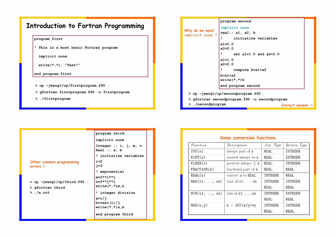
Introduction to Fortran Programming program first ! This is a most basic Fortran program implicit none write(*,*), “Test!” end program first
> cp ~jwang1/cp/firstprogram.f90 . > gfortran firstprogram.f90 -o firstprogram
> ./firstprogram
program second
real:: a1, a2, b!
! initialise variables
a1=0.0 a2=0.0
! set a1=1.0 and a2=2.0
al=1.0 a2=2.0
! compute b=a1+a2
b=a1+a2 write(*,*)b
end program second
> cp ~jwang1/cp/secondprogram.f90 . > gfortran secondprogram.f90 -o secondprogram > ./secondprogram
Why do we need implicit none ?!
implicit none!
Correct answer ?!
program third
implicit none
Integer :: i, j, m, n Real :: a, b!
! initialise variables
i=2 j=3
! exponential
m=2**i**j n=2**j**i write(*,*)m,n !
! integer division
a=i/j b=real(i)/j write(*,*)a,b
end program third
> cp ~jwang1/cp/third.f90 . > gfortran third > ./a.out
Other common programming errors ?!
Write(*,*)a,b
Some conversion functions!

program temperature! implicit none real :: DegC, DegF Write(*,*)"Please type in temp in Celsius" Read(*,*)DegC DegF = (9./5.)*DegC + 32. Write(*,*)"This equals to”,DegF,"Fahrenheit" end program temperature
Converts Celsius to Fahrenheit
> cp ~jwang1/cp/temperature.f90 . > gfortran temperature.f90 -o temperature > temperature
program bouncing_balls ! Use the FD method to compute the trajectory of a bouncing ball ! assuming perfect reflection at the surface x = 0. Use SI units. integer :: steps real :: x, v, g, t, dt x = 1.0 ! initial height of the ball v = 0.0 ! initial velocity of the ball g = 9.8 ! gravitational acceleration t = 0.0 ! initial time dt = 0.01 ! size of time step open(10,file='bounce.dat') ! open data file do steps = 1, 300 ! loop for 300 timesteps t = t + dt x = x + v*dt v = v - g*dt if(x.le.0) then ! reflect the motion of the ball x = -x ! when it hits the surface x=0 v = -v endif write(10,'(3f10.6)') t, x, v ! write out data at each time step enddo end program bouncing_balls
Fortran
v(t +Δt)− v(t)Δt
≈ −g
x(t +Δt)− x(t)Δt
≈ v(t)
�
dv
dt= F m = −g
dx
dt= v
#include <stdio.h> /* standard input-output header */ /* Use the FD method to compute the trajectory of a bouncing ball */ /* assuming perfect reflection at the surface x = 0. Use SI units. */ int main(void) { int steps; float x,v,t,g,dt; FILE* output_file; x = 1.0; /* initial height of the ball */ v = 0.0; /* initial velocity of the ball */ g = 9.8; /* gravitational acceleration */ t = 0.0; /* initial time */ dt = 0.01; /* size of time step */ output_file = fopen("bounce.dat","w"); /* open data file */ for(steps=1;steps<=300;steps++) /* loop for 300 timesteps */ { t += dt; /*shorthand equivalent to t = t+dt */ x += v*dt; v -= g*dt; if(x < 0) /* reflect the motion of the ball */ { /* when it hits the surface x=0 */ x = -x; v = -v; } fprintf(output_file,"%f %.7f %f \n",t,x,v);
/* write out data at each time step */ } fclose(output_file); }
C
v(t +Δt)− v(t)Δt
≈ −g
x(t +Δt)− x(t)Δt
≈ v(t)
�
dv
dt= F m = −g
dx
dt= v
Assignment (due March 12, Tuesday) Exercise 1: Copy the Fortran program to your directory (cp ~jwang1/cp/bouncing.f90 .), compile it to produce an executable file (gfortran bouncing.f90 -o bbf) and run (./bbf). Plot and interpret your results. Are your numerical results physically correct? If not, can you identify a systematic error in the algorithm and then fix the problem? Exercise 2: Copy the C program to your directory (cp ~jwang1/cp/bouncing.c .), compile it to produce an executable file (cc bouncing.c -o bbc) and run (./bbc). Compare with your Fortran results. Exercise 3: Change time step dt in the code (either Fortran or C). Keep the same total evolution time. Explain the changes in the results. Exercise 4: Change the initial velocity and position of the falling ball in the code. Plot and interpret your results. Exercise 5: Consider inelastic collisions with the table (e.g. the ball loses 10% of its speed after each collision). Plot and interpret your results.