computational physics with maxima or r: example 3, time
TRANSCRIPT
Computational Physics with Maxima or R:Example 3, Time Independent Schroedinger’s Equation in 1D∗
Edwin (Ted) Woollett
August 24, 2015
Contents1 Transforming Schroedinger’s Time Independent Equation to Dimensionless Form 3
2 The Finite Rectangular Potential Well: Energy Levels and Wave Functions 42.1 Finite Well Analytic Solution . . . . . . . . . . . . . . . . . . . . . .. . . . . . . . . . . . . . . . . . . . . . . . . . . . . . . . . . . . . . . . 5
2.1.1 Analytic Energies and Wave Functions using Maxima . . .. . . . . . . . . . . . . . . . . . . . . . . . . . . . . . . . . . . . . . . . . . 62.1.2 Analytic Energies and Wave Functions using R . . . . . . . .. . . . . . . . . . . . . . . . . . . . . . . . . . . . . . . . . . . . . . . . 12
2.2 Numerical Runge Kutta Finite Well Solution . . . . . . . . . . .. . . . . . . . . . . . . . . . . . . . . . . . . . . . . . . . . . . . . . . . . . . 192.2.1 Numerical Energies and Wave Functions using Maxima . .. . . . . . . . . . . . . . . . . . . . . . . . . . . . . . . . . . . . . . . . . . 192.2.2 Numerical Energies and Wave Functions using R . . . . . . .. . . . . . . . . . . . . . . . . . . . . . . . . . . . . . . . . . . . . . . . 32
3 The Numerov Integration Method 453.1 Classical Simple Harmonic Oscillator Test Case . . . . . . .. . . . . . . . . . . . . . . . . . . . . . . . . . . . . . . . . . . . . . . . . . . . . 45
3.1.1 Classical SHO Numerov Method Using Maxima . . . . . . . . . .. . . . . . . . . . . . . . . . . . . . . . . . . . . . . . . . . . . . . . 463.1.2 Classical SHO Numerov Method Using R . . . . . . . . . . . . . . .. . . . . . . . . . . . . . . . . . . . . . . . . . . . . . . . . . . . 48
4 The Lennard Jones 6-12 Potential Well: Energy Levels and Wave Functions 504.1 The Numerov Method Using Maxima . . . . . . . . . . . . . . . . . . . . .. . . . . . . . . . . . . . . . . . . . . . . . . . . . . . . . . . . . 504.2 The Numerov Method Using R . . . . . . . . . . . . . . . . . . . . . . . . . .. . . . . . . . . . . . . . . . . . . . . . . . . . . . . . . . . . 64
∗The code examples useR ver. 3.0.2 andMaxima ver. 5.31 usingWindows 7. This is a live document which will be updated when needed.Check http://www.csulb.edu/ ˜ woollett/ for the latest version of these notes. Send comments and suggestions for improvements [email protected]
1

2
COPYING AND DISTRIBUTION POLICYThis document is example3.pdf which applies some of thetopics in the third chapter of a series of notes titledComputational Physics with Maxima or R , and is made availabl evia the author’s webpage http://www.csulb.edu/˜woollett /to encourage the use of the Maxima and R languages for computa tionalphysics projects of modest size.
NON-PROFIT PRINTING AND DISTRIBUTION IS PERMITTED.
You may make copies of this document and distribute themto others as long as you charge no more than the costs of printi ng.
Code files which accompany Example 3 are1. FW.mac finite rectangular well2. FW.R3. LJ6-12.mac Lennard Jones 6/12 potential4. LJ6-12.R
The code files from Chapter 3, cp3.mac and cp3.R, arealso needed to run the examples.
A very useful reference is the new textbook:Computational Physics: A Practical Introduction to Comput ational Physics
and Scientific Computing, Athens, 2014,by Konstantinos Anagnostopoulos.
Free copies in various formats are available on the webpage:http://www.physics.ntua.gr/˜konstant/ComputationalP hysics/
The author’s webpage is:http://www.physics.ntua.gr/˜konstant
Feedback from readers is the best way for this series of notesto become more helpful to users ofR andMaxima. Allcomments and suggestions for improvements will be appreciated and carefully considered.

1 TRANSFORMING SCHROEDINGER’S TIME INDEPENDENT EQUATION TO DIMENSIONLESS FORM 3
1 Transforming Schroedinger’s Time Independent Equation to Dimensionless Form
We assume a scalar particle (spin zero). Using ordinary units, the wave functionψ(x), for one dimensional problems, isa solution of the eigenvalue equation
~2
2m
d2
dx2ψ(x) + (E − V (x)) ψ(x) = 0 (1.1)
in which E is the energy of the particle in ergs,V (x) is the potential energy in ergs, andx is a length in centimeters.The coordinate space wave functionψ(x) is assumed to be normalized according to (integrating over the region in whichψ(x) is nonzero)
∫
|ψ(x)|2 dx = 1, (1.2)
sincedx |ψ(x)|2 is (in the absence of any other information) the probabilitythat the particle described byψ(x) will befound in the interval(x, x+ dx), and the sum of the probabilities of mutually exclusive outcomes must add up to unity.
For Schroedinger’s time independent equation in 1D, we can usually takeψ(x) to be a real function ofx, and from (1.2)we see that the dimension ofψ(x) is 1/
√cm.. Quoting Landau and Lifshitz, Quantum Mechanics, third revised edition
reprinted 2003, p. 55,
Schroedinger’s equation for the wave functionsψ of stationary states is real, as are the conditions imposedon its solution. Hence its solutions can always be taken as real (These assertions are not valid for systems ina magnetic field; it is assumed that the potential energy doesnot depend explicitly on the time: the system iseither closed or in a constant (non-magnetic) field).
The eigenfunctions of non-degenerate values of the energy are automatically real, apart from an unimportantphase factor. . . . The wave functions corresponding to the same degenerate energy level need not be real, butby a suitable choice of linear combinations of them we can always obtain a set of real functions.
We assume there exists a quantityL with the dimensions ofcm., chosen for convenience, in terms of which we can definea dimensionless coordinatex
x = x/L. (1.3)
We also assume there exists an energyV0 (with dimensions ofergs) associated with the potential energy in terms ofwhich we can define a dimensionless potential energyV (x)
V (x) =V (x)
V0(1.4)
and a dimensionless energyE
E =E
V0. (1.5)
We also define a dimensionless coordinate space wave function ψ(x)
ψ(x) =√Lψ(x), (1.6)
in terms of which we have the transformed Schroedinger’s equation
d2 ψ(x)
d x2+ γ2
(
E − V (x))
ψ(x) = 0, (1.7)
where
γ =
√
2mL2 V0~2
, (1.8)

2 THE FINITE RECTANGULAR POTENTIAL WELL: ENERGY LEVELS AND WAVE FUNCTIONS 4
and we have a normalization condition in terms ofx andψ(x):∫
ψ(x)2 d x = 1. (1.9)
The “uncertainty relation” is a condition on the product of the uncertainty∆x in the position of the particle, and theuncertainty∆px in the simultaneousx component of the mechanical momentum of the particle:
∆x∆px ≥ ~
2(1.10)
in which, for a propertyA,∆A =
√
(∆A)2 (1.11)
and(∆A)2 =
⟨
(A− < A >)2⟩
=⟨
A2⟩
− < A >2 . (1.12)
We define a dimensionlessx component of momentumpx
px =L
~px, (1.13)
in terms of which (1.10) becomes
∆x∆px ≥ 1
2. (1.14)
The expectation value ofpnx
〈pnx〉 =∫
ψ∗(x)
(
~
i
d
dx
)n
ψ(x) dx (1.15)
becomes
〈pnx〉 =∫
ψ∗(x)
(
1
i
d
dx
)n
ψ(x) dx. (1.16)
When we can assumeψ(x) is real (most of the time),< px > is either zero or a pure imaginary number, since
< px >=
∫
ψ(x)~
i
dψ(x)
dxdx. (1.17)
But< px > must be real, and thus we conclude it must also be zero. For consistency, this implies that∫
ψ(x)dψ(x)
dxdx = 0. (1.18)
2 The Finite Rectangular Potential Well: Energy Levels and Wave Functions
We assume a finite well such thatV (x) = V0 for x ≤ 0 and also forx ≥ L > 0, while V (x) = 0 for 0 < x < L.Transforming to dimensionless units as described in the previous section, we then haveV (x) = 1 for x ≤ 0 and forx ≥ 1, andV (x) = 0 for 0 < x < 1. In the following, we drop the tildes, withx→ x, V (x) → V (x), E → E, px → px,andψ(x) → y(x), so we are seeking energy eigenvaluesE and the associated energy eigenfunctionsy(x) such thaty(x)is a real continuous function satisfying the equation
d2
dx2y(x) + γ2 (E − V (x)) y(x) = 0 (2.1)
and such thaty(x) → 0 asx→ ±∞ in such a way that we can satisfy the normalization condition∫
∞
−∞
y(x)2 dx = 1, (2.2)
and we also satisfy the basic uncertainty relation∆x∆px ≥ 1
2.

2 THE FINITE RECTANGULAR POTENTIAL WELL: ENERGY LEVELS AND WAVE FUNCTIONS 5
UsingRgraphics methods, we can make a simple plot of the dimensionless rectangular well (which now looks like a finitesquare well), and add a hypothetical energy level (in red).
> setwd("c:/k3")> source("cp3.R")> plot(0, type="n",xlim=c(-2,2),ylim=c(-2,2),xlab="x" ,ylab="V(x)")> lines( c(-2,0), c(1,1), lwd = 3,col = "blue" )> lines( c(0,0), c(0,1), lwd = 3, col = "blue" )> lines( c(0,1), c(0,0), lwd = 3, col = "blue" )> lines( c(1,1), c(0,1), lwd = 3, col = "blue" )> lines( c(1,2), c(1,1), lwd = 3, col = "blue" )> mygrid()> lines( c(0,1), c(0.3,0.3), lwd = 3, col = "red" )
which produces the plot
−2 −1 0 1 2
−2
−1
01
2
x
V(x
)
Figure 1: Dimensionless Finite Well
2.1 Finite Well Analytic Solution
We first seek an analytic solution of the finite well problem. In the regions in whichV (x) = 1, the solutions of (2.1)which vanish for large values of|x| are
y(x) = B1 ek1 x, x ≤ 0, (2.3)
andy(x) = A2 e
−k1 x, x ≥ 1, (2.4)
in whichk1 = γ
√1− E, (2.5)
andB1 andA2 are constants.
The general solution in the region in whichV (x) = 0 can be written in the form
y(x) = A sin(k x+ δ), 0 ≤ x ≤ 1, (2.6)
in whichk = γ
√E. (2.7)
2 THE FINITE RECTANGULAR POTENTIAL WELL: ENERGY LEVELS AND WAVE FUNCTIONS 6
This last equation can be solved forE:
E =k2
γ2. (2.8)
We can also then expressk1 in terms ofk:k1 =
√
γ2 − k2. (2.9)
The required continuity of bothy andy′ implies the continuity of the ratioy′/y. We have
y′(x)
y(x)= k1, x ≤ 0, (2.10)
andy′(x)
y(x)= −k1, x ≥ 1, (2.11)
andy′(x)
y(x)= k cot(k x+ δ), 0 ≤ x ≤ 1. (2.12)
Then the continuity ofy′/y atx = 0 implies
tan(δ) =k
k1=
k√
γ2 − k2. (2.13)
And the continuity ofy′/y atx = 1 implies
tan(k + δ) = − k
k1= − tan(δ). (2.14)
We expand the left hand side of this last equation, using the identity
tan(A+B) =tan(A) + tan(B)
1− tan(A) tan(B), (2.15)
and use again (2.13) to get
k =(2 k2 − γ2)
2√
γ2 − k2tan(k). (2.16)
This equation will involve real numbers provided we have
0 < k < γ. (2.17)
We can search for values ofk which satisfy both (2.16) and (2.17), which will then imply corresponding energy eigen-values using (2.8). A graphical search can be achieved by plotting the left and right hand sides of (2.16) on the same plotand looking for intersections.
2.1.1 Analytic Energies and Wave Functions using Maxima
Our functionkroot_plot(kkmin,kkmax,ymn,ymx) (available for use once the code fileFW.mac is loaded) is de-signed to partially automate such a graphical search.
Frhs(k) := (float( (2 * kˆ2 - gam2) * tan(k)/2/sqrt(gam2 - kˆ2)) )$
kroot_plot(kkmin,kkmax, ymn, ymx) :=( plot2d([kk, Frhs(kk)], [kk, kkmin, kkmax],
[y, ymn, ymx], [style, [lines,2]], [xlabel, "k"],[legend, false], [ylabel, ""],
[gnuplot_preamble," set grid"]))$

2 THE FINITE RECTANGULAR POTENTIAL WELL: ENERGY LEVELS AND WAVE FUNCTIONS 7
After loadingFW.mac, gam2 is a global parameter which stands forγ2, and in this code file we useγ = 50.
(%i1) load(cp3);(%o1) "c:/k3/cp3.mac"(%i2) load(FW);
gam = 50 gam2 = 2500h = 0.01 , xdecay = 0.5 , ypleft = 1.0E-8 ypright = 1.0E-8
(%o2) "c:/k3/FW.mac"(%i3) kroot_plot(1,49,0,60)$plot2d: some values were clipped.
which produces the plot
0
10
20
30
40
50
60
5 10 15 20 25 30 35 40 45
k
Figure 2: Graphical Search for k Roots
Placing the cursor over the intersections of the curves, we see that k roots occur approximately at valuesk = 3.01, 6.03, 9.06,... .
Fa(k) is a function, also defined inFW.mac, which is zero at these special values ofk . Also defined isktoE(k) whichconvertsk to E.
Fa(k) := (float(k - (2 * kˆ2 - gam2) * tan(k)/2/sqrt(gam2 - kˆ2)) )$
ktoE (kv) := (kvˆ2/gam2)$
This functionFa(k) (of one variable) can then be directly used with the core Maxima functionfind_root to find theground state energyE0.
(%i4) Fa(2.9);(%o4) -3.2290071(%i5) Fa(3.1);(%o5) 2.0655923(%i6) k0 : find_root(Fa,2.9,3.1);(%o6) 3.0206914(%i7) E0 : ktoE(k0);(%o7) 0.00364983(%i8) plot_analytic(E0)$
E = 0.00364983x_mean = 0.5delx = 0.18802ydy_sum = -1.78676518E-16delp = 2.9619274 delx * delp = 0.556902number of nodes = 0

2 THE FINITE RECTANGULAR POTENTIAL WELL: ENERGY LEVELS AND WAVE FUNCTIONS 8
which produces the plot of the normalized analytic ground state wave function with zero nodes.
0
0.5
1
1.5
2
-0.5 0 0.5 1 1.5
yna(
x)
x
Figure 3: Analytic Normalized Ground State Wave Function
The functionplot_analytic(E) (see below) callsanalytic_wf(E) (see code fileFW.mac), and the latter file cal-culatesdelx , delp , x_mean, andydy_sum . The calculated value ofydy_sum corresponds to the integral (1.18) whichshould be zero.
The functionfind_root also appears to find a spurious root at or nearπ/2 which is not a physical solution. The function
Fa(k) = k − (2 k2 − γ2)
2√
γ2 − k2tan(k). (2.18)
is not a continuous function atk = n π2, n = 1, 3, 5, . . . wheretan(k) is not continuous, andfind_root cannot be
trusted at such points. For example,
(%i9) Fa(1.55);(%o9) 1201.7787(%i10) Fa(1.59);(%o10) -1298.109(%i11) k0s : find_root(Fa,1.55,1.59);(%o11) 1.5707963(%i12) Fa(k0s);(%o12) 4.07689764E+17(%i13) E0s : ktoE(k0s);(%o13) 9.8696044E-4(%i14) plot_analytic(E0s)$
E = 9.8696044E-4x_mean = 0.700405delx = 0.212493ydy_sum = 2.22044605E-16delp = 6.6877608 * (-1)ˆ0.5 delx * delp = 1.4210999 * (-1)ˆ0.5number of nodes = 0

2 THE FINITE RECTANGULAR POTENTIAL WELL: ENERGY LEVELS AND WAVE FUNCTIONS 9
which produces the plot of a discontinuous zero node wave function:
0
0.5
1
1.5
2
-0.5 0 0.5 1 1.5
yna(
x)
x
Figure 4: Discontinuous Spurious Root Wave Function
Note also the calculation produced a purely imaginary valuefor delp . Note also the large value ofFa(k0s) , whichshould be a very small number close to a physical root.
The functionanalytic_wf(E) creates global analytic normalized wave functionsyn1(x) , yn2(x) , yn0(x) , andyna(x) ( and also computes and prints analytic values of∆x, represented bydelx , and∆p, represented bydelp ).yn1(x) is the wave function forx < 0, yn2(x) is the wave function forx > 1, yn0(x) is the wave function for0 ≤ x ≤ 1. yna(x) is the wave function for allx, usable byplot2d , but not byintegrate , created by the line
yna(x) :=( if x < 0 then yn1(x)
else if x > 1 then yn2(x)else yn0(x) ),
Ignoring normalization, one can write a continuousyu(x) as
yu(x) = sin(δ) ek1 x, x ≤ 0, k1 = γ√1− E
= sin(k x+ δ), 0 ≤ x ≤ 1, k = γ√E
= sin(k + δ) ek1 e−k1 x, x ≥ 1.
Normalization then requires calculating
D =
∫
∞
−∞
y2u(x) dx. (2.19)
and a normalized wave functionyn(x) is then
yn(x) =yu(x)√D. (2.20)
The functionplot_analytic(E) used above callsanalytic_wf(E) and nodes_analytic(ddx) , prints out thenumber of nodes, and makes a plot ofyna(x) .
plot_analytic(E) :=block ( [ddx : 0.001, xvL, ynL, ymn, ymx,
xmn: -0.25, xmx : 1.25, numer], numer:true,analytic_wf(E),xvL : makelist(x,x,0,1,ddx),ynL : map(yn0, xvL),ymn : floor( lmin(ynL) ),

2 THE FINITE RECTANGULAR POTENTIAL WELL: ENERGY LEVELS AND WAVE FUNCTIONS 10
ymx : 1 + floor( lmax (ynL) ),print(" number of nodes = ", nodes_analytic(ddx) ),plot2d(yna(x), [x,xmn,xmx], [ylabel, "yna(x)"],[y,ymn, ymx],
[style,[lines,2]],[gnuplot_preamble,"set grid"]))$
The functionnodes_analytic(dx) counts the number of nodes implied by the functionyn0(x) created byanalytic_wf(E) . The count is naturally restricted to the region0 ≤ x ≤ 1 and the argumentdx is the step size used.
nodes_analytic ( dx ) :=block( [num:0, xv:0, xnew, f1, f2, numer], numer:true,
do (f1 : yn0(xv),xnew : xv + dx,if xnew > 1 then return(),f2 : yn0(xv + dx),if f1 * f2 < 0 then num : num + 1,xv : xnew),
num)$
A function levels_analytic(kmax) returns a list of analytic eigen energies related tok via k = γ√E. The corre-
sponding eigenvalues ofk are separated by roughlydk = 3 and lie in the middle of the intervals[n1 π2, n2
π2], wheren1 and
n2 are adjacent odd integers withn2 > n1. The ground state (zero node soln) corresponds tok = 3.02, n1 = 1, n2 = 3.
levels_analytic(kmax) :=block( [ka,kb,kv,level:0, nmax, Elist : [], numer], numer: true,
nmax : ceiling(2 * kmax/%pi),print(" nodes E "),print( " "),/ * make nmax an odd integer * /if evenp (nmax) then nmax : nmax + 1,/ * analytic kv using n * pi/2 + 0.1 with n odd * /for j:1 step 2 thru nmax do (
[ka, kb] : bracket_basic( Fa, j * %pi/2 + 0.1, 0.01, 0.005),kv : find_root( Fa, ka, kb),Ev : ktoE(kv),Elist : cons(Ev, Elist),print( " ", level, " ", Ev ),level : level + 1),
reverse(Elist) )$
Here is an example of the use oflevels_analytic :
(%i15) levels_analytic(20);nodes E
0 0.003649831 0.01459732 0.0328363 0.05835524 0.09113895 0.1311656 0.178405
(%o15) [0.00364983,0.0145973,0.032836,0.0583552,0.09 11389,0.131165,0.178405](%i16) E4 : %[5];(%o16) 0.0911389(%i17) plot_analytic(E4)$
E = 0.0911389x_mean = 0.5delx = 0.297122ydy_sum = -8.32667268E-17delp = 14.787571 delx * delp = 4.3937127number of nodes = 4

2 THE FINITE RECTANGULAR POTENTIAL WELL: ENERGY LEVELS AND WAVE FUNCTIONS 11
which produces the plot
-2
-1.5
-1
-0.5
0
0.5
1
1.5
2
-0.5 0 0.5 1 1.5
yna(
x)
x
Figure 5: Analytic Four Node Wave FunctionE = 0.0911389
The functionlevels_analytic calls bracket_basic(func,x,dx,xacc) which looks for a sign change infunc ,starting withx, and increasingx by dx each step. If a sign change is found, then we back up to the previousx and searchwith newdx value one half of the previous value.
bracket_basic(func,xx,dxx,xacc) :=block([ x:xx, dx:dxx,x1,x2,it:0,itmax:1000],
do (it : it + 1,if it > itmax then (print(" can’t find change in sign "),
return([0, 0 ])),x1 : x,x2 : x + dx,if debug then print(" it = ",it," x1 = ",x1," x2 = ",x2," dx = ", d x),
if func(x1) * func(x2) < 0 then (if abs(dx) < xacc then return([x1,x2]),
x : x - dx,dx : dx/2)
else x : x2))$
Here is an example usingbracket_basic with func = sin :
(%i18) [xa,xb] : bracket_basic(sin,3,0.01,0.001);(%o18) [3.14125,3.141875](%i19) xv : find_root(sin,xa,xb);(%o19) 3.1415927
Here is an example of locating the zero node ground state value ofk for the finite potential well problem usingfunc = Fa
(see (2.18)).
(%i20) [ka,kb] : bracket_basic(Fa,1.6,0.1,0.05);(%o20) [3.0,3.025](%i21) kv : find_root(Fa,ka,kb);(%o21) 3.0206914
2 THE FINITE RECTANGULAR POTENTIAL WELL: ENERGY LEVELS AND WAVE FUNCTIONS 12
2.1.2 Analytic Energies and Wave Functions using R
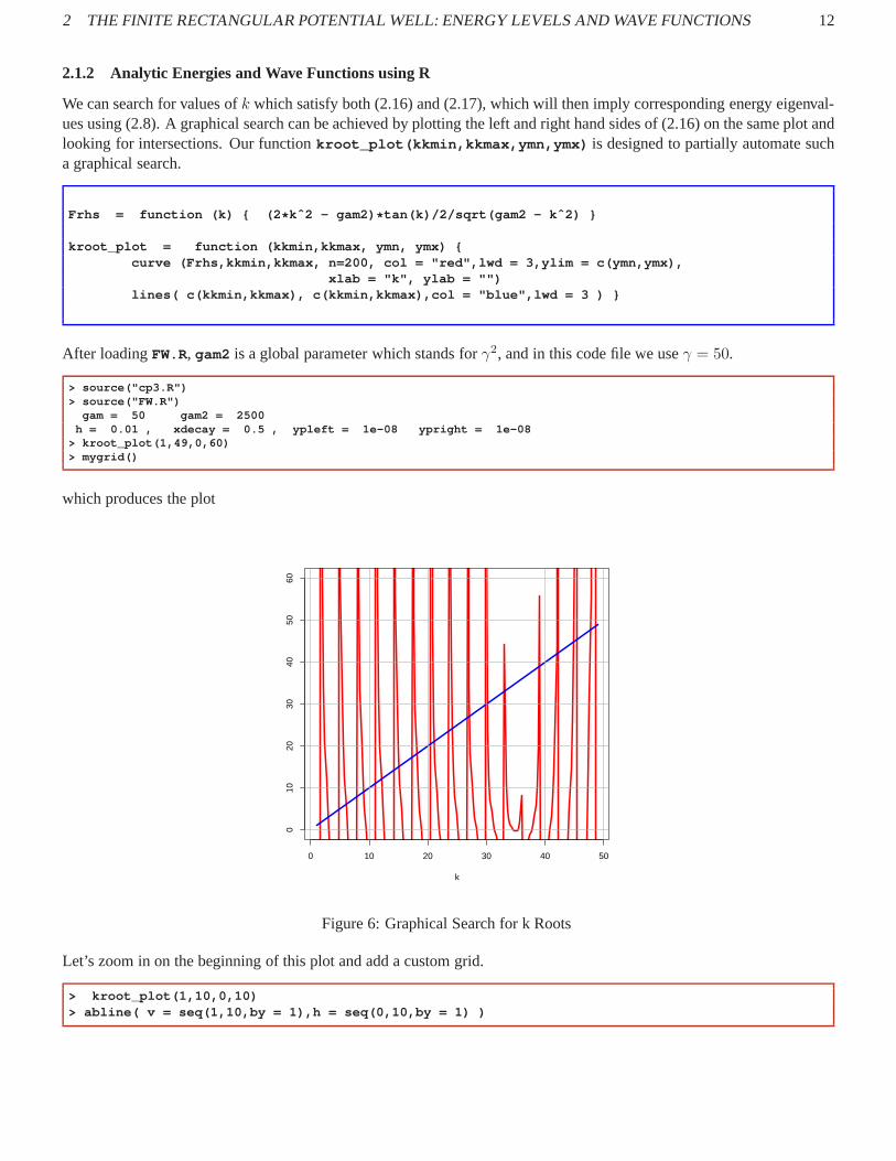
We can search for values ofk which satisfy both (2.16) and (2.17), which will then imply corresponding energy eigenval-ues using (2.8). A graphical search can be achieved by plotting the left and right hand sides of (2.16) on the same plot andlooking for intersections. Our functionkroot_plot(kkmin,kkmax,ymn,ymx) is designed to partially automate sucha graphical search.
Frhs = function (k) { (2 * kˆ2 - gam2) * tan(k)/2/sqrt(gam2 - kˆ2) }
kroot_plot = function (kkmin,kkmax, ymn, ymx) {curve (Frhs,kkmin,kkmax, n=200, col = "red",lwd = 3,ylim = c (ymn,ymx),
xlab = "k", ylab = "")lines( c(kkmin,kkmax), c(kkmin,kkmax),col = "blue",lwd = 3 ) }
After loadingFW.R, gam2 is a global parameter which stands forγ2, and in this code file we useγ = 50.
> source("cp3.R")> source("FW.R")
gam = 50 gam2 = 2500h = 0.01 , xdecay = 0.5 , ypleft = 1e-08 ypright = 1e-08
> kroot_plot(1,49,0,60)> mygrid()
which produces the plot
0 10 20 30 40 50
010
2030
4050
60
k
Figure 6: Graphical Search for k Roots
Let’s zoom in on the beginning of this plot and add a custom grid.
> kroot_plot(1,10,0,10)> abline( v = seq(1,10,by = 1),h = seq(0,10,by = 1) )

2 THE FINITE RECTANGULAR POTENTIAL WELL: ENERGY LEVELS AND WAVE FUNCTIONS 13
which produces the plot
2 4 6 8 10
02
46
810
k
Figure 7: Graphical Search for k Roots
Physically valid k roots occur roughly at values slightly larger thank = 3, 6, 9, . . .. The vertical red lines correspond tovalues ofk = π/2, 3π/2, . . . wheretan(k) both changes sign and has an arbitrarily large magnitude. The intersectionswith the vertical red lines are not physically valid roots, as we will see.
An function which should be zero at a physical root is calledFa(k) and we also definektoE(k) , which convertsk to E.
Fa = function(k) { k - (2 * kˆ2 - gam2) * tan(k)/2/sqrt(gam2 - kˆ2) }
ktoE = function (k) kˆ2/gam2
This functionFa(k) (of one variable) can then be directly used withuniroot to find the ground state energyE0.
> Fa(2.9)[1] -3.22901> Fa(3.1)[1] 2.06559> k0 = uniroot(Fa, c(2.9, 3.1), tol=1e-16)$root> k0[1] 3.02069> E0 = ktoE(k0)> E0[1] 0.00364983> plot_analytic(E0)
E = 0.00364983x_mean = 0.5delx = 0.18802ydy_sum = -1.78677e-16delp = 2.96193 delx * delp = 0.556902ymn = 0 ymx = 2number of nodes = 0

2 THE FINITE RECTANGULAR POTENTIAL WELL: ENERGY LEVELS AND WAVE FUNCTIONS 14
which produces the plot of the normalized analytic ground state wave function with zero nodes.
0.0 0.5 1.0
0.0
0.5
1.0
1.5
2.0
x
ya(x
)
Figure 8: Analytic Normalized Ground State Wave Function
The functionuniroot also appears to find a spurious root at or nearπ/2 which is not a physical solution. Thefunction
Fa(k) = k − (2 k2 − γ2)
2√
γ2 − k2tan(k). (2.21)
is not a continuous function atk = n π2, n = 1, 3, 5, . . . wheretan(k) is not continuous, anduniroot cannot be
trusted at such points. For example,
> Fa(1.55)[1] 1201.78> Fa(1.59)[1] -1298.11> k0s = uniroot(Fa,c(1.55,1.59),tol=1e-16)$root> k0s[1] 1.5708> Fa(k0s)[1] -3.01869e+16> E0s = ktoE(k0s)> E0s[1] 0.00098696> plot_analytic(E0s)
E = 0.00098696x_mean = 0.700405delx = 0.212493ydy_sum = 1.11022e-16delp = NaN delx * delp = NaNymn = 0 ymx = 2number of nodes = 0
Warning message:In sqrt(delp2) : NaNs produced

2 THE FINITE RECTANGULAR POTENTIAL WELL: ENERGY LEVELS AND WAVE FUNCTIONS 15
which produces the plot of a discontinuous zero node wave function:
0.0 0.5 1.0
0.0
0.5
1.0
1.5
2.0
x
ya(x
)
Figure 9: Discontinuous Spurious Root Wave Function
Note also the calculation produced a purely imaginary valuefor delp , whichR writes asNaN(not a number). Note alsothe large value ofFa(k0s) , which should be a very small number close to a physical root.
The functionanalytic_wf(E) creates global analytic normalized wave functionsyn1(x) , yn2(x) , yn0(x) , andyna(x) ( and also computes and prints analytic values of∆x, represented bydelx , and∆p, represented bydelp ).yn1(x) is the wave function forx < 0, yn2(x) is the wave function forx > 1, yn0(x) is the wave function for0 ≤ x ≤ 1. yna(x) is the wave function for allx, usable bysapply , but not bycurve , created by the line
yna <<- function (x) { if (x < 0) yn1(x) else if (x > 1) yn2(x) els e yn0(x) }
Ignoring normalization, one can write a continuousyu(x) as
yu(x) = sin(δ) ek1 x, x ≤ 0, k1 = γ√1− E
= sin(k x+ δ), 0 ≤ x ≤ 1, k = γ√E
= sin(k + δ) ek1 e−k1 x, x ≥ 1.
Normalization then requires calculating
D =
∫
∞
−∞
y2u(x) dx. (2.22)
and a normalized wave functionyn(x) is then
yn(x) =yu(x)√D. (2.23)
The functionplot_analytic(E) used above callsanalytic_wf(E) and nodes_analytic(ddx) , prints out thenumber of nodes, and makes a plot ofyna(x) .
plot_analytic = function (E) {ddx = 0.001xmn = - 0.25xmx = 1.25

2 THE FINITE RECTANGULAR POTENTIAL WELL: ENERGY LEVELS AND WAVE FUNCTIONS 16
analytic_wf(E)xL = seq(xmn,xmx ,by = ddx)yL = sapply(xL, yna)ymn = floor( min(yL) )ymx = 1 + floor( max (yL) )cat (" ymn = ",ymn," ymx = ",ymx, "\n")cat (" number of nodes = ", nodes_analytic(ddx), "\n" )plot(xL, yL, type = "l", lwd = 3, col = "blue", xlab = "x",
ylab = "ya(x)",tck=1, ylim = c(ymn,ymx) ) }
The functionnodes_analytic(dx) , used above, counts the number of nodes implied by the function yn0(x) createdby analytic_wf(E) . This function looks in the region0 ≤ x ≤ 1, using intervals of sizedx .
nodes_analytic = function ( dx ) {num = 0xv = 0repeat {
f1 = yn0(xv)xnew = xv + dxif (xnew > 1) breakf2 = yn0(xv + dx)if (f1 * f2 < 0 ) num = num + 1xv = xnew }
num }
A function levels_analytic(kmax) returns a list of analytic energy eigenvalues related tok via k = γ√E. The
corresponding eigenvalues ofk are separated by roughlydk = 3 and lie in the middle of the intervals[n1 π2, n2
π2], where
n1 andn2 are adjacent odd integers withn2 > n1. The ground state solution corresponds tok = 3.02, n1 = 1, n2 = 3.
levels_analytic = function (kmax) {rmax = 20EL = rep(NA, rmax)level = 0nmx = ceiling(2 * kmax/pi)## make nmx an odd integerif ( is.even (nmx) ) nmx = nmx + 1cat (" nodes E \n ")cat ( " \n ")
## analytic kv using n * pi/2 + 0.1 with n oddfor ( j in seq(1, nmx, by=2) ) {
out = bracket_basic( Fa, j * pi/2 + 0.1, 0.01,0.005)kv = uniroot( Fa, out, tol = 1e-16)$rootEv = ktoE(kv)EL[ j ] = Evcat ( " ", level, " ", Ev, "\n" )level = level + 1 }
EL[!is.na(EL)] }
Here is an example of the use oflevels_analytic :
> EL = levels_analytic(20)nodes E
0 0.003649831 0.01459732 0.0328363 0.05835524 0.09113895 0.1311656 0.178405

2 THE FINITE RECTANGULAR POTENTIAL WELL: ENERGY LEVELS AND WAVE FUNCTIONS 17
> EL[1] 0.00364983 0.01459726 0.03283598 0.05835517 0.091138 90 0.13116525 0.17840502> E4 = EL[5]> E4[1] 0.0911389> plot_analytic(E4)
E = 0.0911389x_mean = 0.5delx = 0.297122ydy_sum = -8.32667e-17delp = 14.7876 delx * delp = 4.39371ymn = -2 ymx = 2number of nodes = 4
which produces the plot
0.0 0.5 1.0
−2
−1
01
2
x
ya(x
)
Figure 10: Analytic Four Node Wave FunctionE = 0.0911389
The functionlevels_analytic calls bracket_basic(func,x,dx,xacc) which looks for a sign change infunc ,starting withx, and increasingx by dx each step. If a sign change is found, then we back up to the previousx and searchwith newdx value one half of the previous value. Note thatdebug = FALSE is set when loading the fileFW.R.
bracket_basic = function (func,xx,dxx,xacc) {x = xxdx = dxxit = 0itmax = 1000anerror = FALSE
repeat {it = it + 1if (it > itmax) {cat (" can’t find change in sign \n")
anerror = TRUEbreak}
x1 = xx2 = x + dxif ( debug ) cat (" it = ",it," x1 = ",x1," x2 = ",x2," dx = ", dx, "\ n")
2 THE FINITE RECTANGULAR POTENTIAL WELL: ENERGY LEVELS AND WAVE FUNCTIONS 18
if (func(x1) * func(x2) < 0 ) {if ( abs(dx) < xacc ) breakx = x - dxdx = dx/2 } else x = x2 }
if (anerror ) c(0,0) else c(x1,x2) }
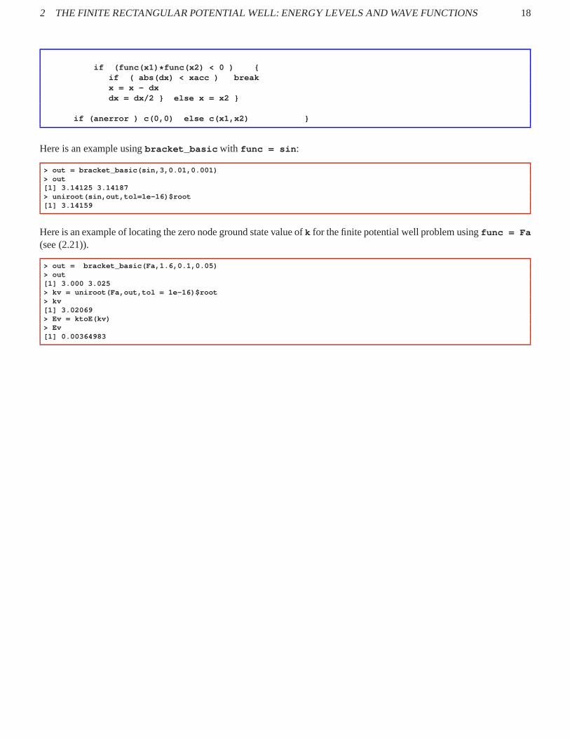
Here is an example usingbracket_basic with func = sin :
> out = bracket_basic(sin,3,0.01,0.001)> out[1] 3.14125 3.14187> uniroot(sin,out,tol=1e-16)$root[1] 3.14159
Here is an example of locating the zero node ground state value ofk for the finite potential well problem usingfunc = Fa
(see (2.21)).
> out = bracket_basic(Fa,1.6,0.1,0.05)> out[1] 3.000 3.025> kv = uniroot(Fa,out,tol = 1e-16)$root> kv[1] 3.02069> Ev = ktoE(kv)> Ev[1] 0.00364983

2 THE FINITE RECTANGULAR POTENTIAL WELL: ENERGY LEVELS AND WAVE FUNCTIONS 19
2.2 Numerical Runge Kutta Finite Well Solution
It is easiest to use Runge-Kutta methods for a case in which the potentialV (x) is discontinuous at one or more values ofx. In this exampleV (x) is discontinuous atx = 0 andx = 1. The Runge-Kutta method automatically supplies the firstderivatives at the spatial grid pointsxL .
2.2.1 Numerical Energies and Wave Functions using Maxima
We use our homemaderk4 routine for the Runge-Kutta integration. When the fileFW.mac is loaded, a number of globalparameters are defined. The top the the fileFW.machas the lines:
/ * FW.mac uses Runge-Kuttafor finite well.
dimensionless unitsV = 1 for x < 0 and x > 1V = 0 for 0 < x < 1y’’(x) + gam2 * (E - V(x)) * y(x) = 0gam2 = gamˆ2 = 2500gam = 50 = sqrt(2 * m* Lˆ2 * V0/ hbarˆ2)
* /
/ * initial global parameters: * /
( N : 100,h : 0.01,gam : 50,gam2 : gamˆ2,xdecay : 0.5, / * start yL1 integration at x = -xdecay * /
/ * start yR integration at x = 1 + xdecay * /ypleft : 1e-8,ypright : 1e-8,print(" gam = ",gam, " gam2 = ", gam2),print(" h = ", h, ", xdecay = ", xdecay, ", ypleft = ",
ypleft," ypright = ", ypright))$
We integrate from a pointx = -xdecay chosen so that we can assumey(-xdecay) = 0 to the pointx = 0, thusdefining a gridxL1 of integration points, a listyL1 of values ofy(x) at these grid points, and a listypL1 of values ofy′(x) at these grid points whereV = 1.
We assume an arbitrary small valueypleft for the first derivativey′ at this starting point. The resulting wave function,the solution of a homogeneous equation, can be later normalized, which will, in effect, amount to choosing the correctinitial first derivative at the left starting point.
The final value ofy andy′ thus generated become the initial values ofy andy′ for integration through the region whereV = 0, 0 ≤ x ≤ 1, thus generating a gridxL2 of integration points, a listyL2 of values ofy(x) at these grid points, anda list ypL2 of values ofy′(x) at these grid points whereV = 0.
The integration in the regionx > 1 is done by starting at a locationx = 1 + xdecay where we can assumey = 0and we again assign an arbitrary (but negative) first derivative - ypright . We then integrate toward smaller values ofxuntil we reachx = 1. Since we are hence integrating in the direction in which thephysical solution is growing, we avoidintegration instability problems produced by small roundoff and integration algorithm errors.
We then multiply the listsyL1 , ypL1 , yL2 , andypL2 by a factor which assures us that the final value ofy(x) producedby the independent rightward and leftward integrations agree at the matching pointx = 1. The value ofy(x) can be madeto agree at the matching point for any energyE. However, the resulting wave function values will still be discontinuous
2 THE FINITE RECTANGULAR POTENTIAL WELL: ENERGY LEVELS AND WAVE FUNCTIONS 20
because the first derivatives will not agree at the matching point.
The crucial step, then, is to design a functionF (E), say, that is zero (to within numerical errors) when the derivativesagree at the matching point. We can then look for the locations of sign changes inF (E) to locate the energy eigenvalues.
The first step needed, in order to be able to design such a function F(E) , is to design a functionwf(E) which uses RungeKutta methods to find a un-normalized wave function corresponding to a given total energyE. Here is our code for sucha wave function integrator, as listed inFW.mac.
/ * wf(E) creates ** un-normalized ** numerical wave functionsusing Runge-Kutta routine rk4.The wave functions are stored in global xL1, yL1,ypL1, xL2, y L2, ypL2, xR, yR, ypR .
Program also defines ** global ** nleft, nright, ncenterthe global xL1 grid extends from -xdecay to 0 andthe global xL2 grid extends from 0 to 1 andthe global xR grid extends from 1 to 1 + xdecay
* /
wf(E) :=block([ glr,gc, outL, fac, numer], numer : true,
if (E < 0) or (E > 1) then (print(" need 0 < E < 1 "),return(false)),
ncenter : N,if not integerp(ncenter) then (
print (" ncenter = ",ncenter," is not an integer"),return(false)),
nleft : round(xdecay/h),nright : nleft,if wfdebug then print(" nleft = ",nleft," ncenter = ",ncente r," nright = ",nright),
glr : gam2 * (E - 1), / * g(x) for x < 0 and x > 1 * /gc : gam2 * E, / * g(x) for 0 < x < 1 * /if wfdebug then print(" glr = ",glr," gc = ", gc),
/ * construct xL1, yL1, and ypL1 for -xdecay < x < 0 * /
outL : rk4([’y2, - glr * ’y1], [’y1, ’y2], [ 0, ypleft], [’x, -xdecay, 0, h] ),xL1 : take(outL,1),yL1 : take(outL,2),ypL1 : take(outL,3),
/ * construct xL2, yL2, and ypL2 for 0 < x < 1 * /
outL : rk4([’y2, - gc * ’y1], [’y1, ’y2], [ last(yL1), last(ypL1)], [’x, 0, 1, h] ),xL2 : take(outL,1),yL2 : take(outL,2),ypL2 : take(outL,3),
/ * construct xR, yR, and ypR for 1 < x < 1 + xdecay * /
outL : rk4([’y2, - glr * ’y1], [’y1, ’y2], [ 0, -ypright], [’x, 1 + xdecay, 1, -h] ),xR : take(outL,1),yR : take(outL,2),ypR : take(outL,3),
xR : reverse(xR),yR : reverse(yR),ypR : reverse(ypR),if wfdebug then print(" yR(1) = ", first(yR)),

2 THE FINITE RECTANGULAR POTENTIAL WELL: ENERGY LEVELS AND WAVE FUNCTIONS 21
fac : first(yR)/last(yL2),if wfdebug then print(" fac = ",fac),
yL1 : fac * yL1,ypL1 : fac * ypL1,yL2 : fac * yL2,ypL2 : fac * ypL2,
done)$
The second step needed to designF(E) is to create a functiondy_diff() which returns a normalized difference of thefirst derivativesy′L(x) − y′R(x) evaluated at the matching pointx = 1. We return this difference divided by the value ofy(x = 1).
/ * dy_diff() uses global ypL2, ypR, and yR,returns a normalized difference of derivatives
(yL’(1) - yR’(1)/ yR(1)
* /
dy_diff() :=block([dy_left, dy_right, numer],numer:true,
dy_left : last(ypL2),dy_right : first(ypR),(dy_left - dy_right)/abs(first(yR)) )$
For example,
(%i1) load(cp3);(%o1) "c:/k3/cp3.mac"(%i2) load(FW);
gam = 50 gam2 = 2500h = 0.01 , xdecay = 0.5 , ypleft = 1.0E-8 ypright = 1.0E-8
(%o2) "c:/k3/FW.mac"(%i3) wf(0.5);(%o3) done(%i4) dy_diff();(%o4) 35.071714(%i5) last(ypL2);(%o5) -0.00190471(%i6) first(ypR);(%o6) -0.237432(%i7) first(yR);(%o7) 0.00671558
Here, finally, is our code forF(E) :
/ * energy eigenvalue if global function F(E) = 0 .F(E) calls wf(E) then returns dy_diff(), but
returns false if E > 0.
* /
F(E) :=block( [ numer],numer:true,
if E < 0 or E > 1 then (print(" in F(E), E = ",E," should be between 0 and 1 "),return(false)),
wf(E),dy_diff())$
And here is an example of usingF(E) to produce a rough graphical survey of the possibilities:

2 THE FINITE RECTANGULAR POTENTIAL WELL: ENERGY LEVELS AND WAVE FUNCTIONS 22
(%i8) EL : makelist(e,e,0.1,0.9,0.01)$(%i9) FL : map(F, EL)$(%i10) plot2d([discrete,EL,FL],[xlabel,"E"],[ylabel, "F(E)"])$
which produces the plot
-400
-200
0
200
400
600
800
1000
0.1 0.2 0.3 0.4 0.5 0.6 0.7 0.8 0.9 1
F(E
)
E
Figure 11: Crude Plot of F(E)
We can useF(E) to search for energy eigenvalue candidates. We do this with afunctionbracket(func,x,dx,xacc)
which attempts to return two values ofx at whichfunc has the opposite sign.
/ * bracket is a modified version of bracket_basic, designed to work withthe function F(E) or F1(k) which can return ’false’.
bracket looks for a sign change in func,starting with xx, and increasing xx by dxx each step.If sign change is found, then we back up to the previous xxand search with new dxx value one half of the previous value.normally returns [ea,eb] or [ka,kb], but if can’t find chang e in sign,then returns [0,0], and if func returns false, thenbracket returns false.
* /
bracket(func,xx,dxx,xacc) :=block([f1,f2, x:xx, dx:dxx,xx1,xx2,it:0,itmax:1000],
do (it : it + 1,if debug then print(it),if it > itmax then (
print(" can’t find change in sign "),return([0, 0 ])),
xx1 : x,xx2 : x + dx,
if debug then print(" it = ",it," xx1 = ",xx1," xx2 = ",xx2," dx = ", dx),f1 : func(xx1),if not f1 then (
print(" in bracket, f1 = false , xx1 = ",xx1, " dx = ", dx),return(f1)),
f2 : func(xx2),

2 THE FINITE RECTANGULAR POTENTIAL WELL: ENERGY LEVELS AND WAVE FUNCTIONS 23
if not f2 then (print(" in bracket, f2 = false , xx2 = ",xx2, " dx = ", dx),return(f2)),
if debug then print (" f1 = ",f1," f2 = ",f2),if f1 * f2 < 0 then (
if abs(dx) < xacc then return([xx1,xx2]),x : x - dx,dx : dx/2)
else x : xx2) )$
Here is an example of usingbracket with the functionF(E) . This example produces the zero node ground state case,and we plot the un-normalized wave function pieces producedby wf(E) .
(%i11) [ea,eb] : bracket(F,0.0005,0.0001,0.00005);(%o11) [0.003625,0.00365](%i12) e : find_root(F,ea,eb);(%o12) 0.00364983(%i13) wf(e);(%o13) done(%i14) plot2d([[discrete,xL1,yL1],[discrete,xL2,yL2] ,[discrete,xR,yR]],
[xlabel,"x"],[ylabel,"y(x)"], [legend,false])$
which produces a plot of the un-normalized ground state wavefunction with zero nodes.
0
20
40
60
80
100
120
-0.5 0 0.5 1 1.5
y(x)
x
Figure 12: Numerical Un-normalized Ground State Wave Function
We can check the normalized difference in slopes at the matching point for the solution produced bywf(E) :
(%i15) dy_diff();(%o15) -2.49565076E-14
We can check the number of nodes with the functionnum_nodes() .
/ * count the number of nodes in yL2 * /
num_nodes() :=block([ n, numer], numer:true,
n : 0,for j thru (length(yL2) - 1) do
if yL2[ j ] * yL2[ j + 1 ] < 0 then n : n + 1,n)$
For the numerical ground state solution generated above bywf(E) we get:

2 THE FINITE RECTANGULAR POTENTIAL WELL: ENERGY LEVELS AND WAVE FUNCTIONS 24
(%i16) num_nodes();(%o16) 0
A functionnormalize() uses the current wave function pieces produced bywf(E) and uses our Simpson’s rule functionsimp to produce global normalized wave function (lists)xn andyn . normalize() uses our functionmerge(aL1,aL2)
to combine the separate lists into one list. After callingnormalize() , one can check the normalization:
(%i17) normalize()$AA = 6652.6824x_mean = 0.5delx = 0.18802
(%i18) simp(xn,ynˆ2);(%o18) 1.0
Here is the code fornormalize() .
/ * normalize() uses the current global xL1,yL1, xL2,yL2, xR, y R andthe utility functions merge and simp to define globalxn and yn, with the latter being normalized.
* /
normalize() :=block ( [AA,x_mean,x2_mean,delx,delx2, numer ], numer:tr ue,
xn : merge( xL1, merge( rest(xL2), rest(xR))),yn : merge( yL1, merge( rest(yL2), rest(yR))),
/ * we need xn to have odd # of elements to use simp * /if evenp ( length (xn) ) then (
xn : rest (xn),yn : rest (yn)),
if debug then print ( " fll(xn) = ", fll(xn) ),if debug then print( " fll(yn) = ", fll(yn) ),AA : simp(xn,ynˆ2),print( " AA = ",AA),yn : yn/sqrt(AA),if debug then print( " fll(yn) = ", fll(yn) ),
x_mean : simp(xn, xn * ynˆ2),print(" x_mean = ", x_mean),x2_mean : simp(xn, xnˆ2 * ynˆ2),
delx2 : x2_mean - x_meanˆ2, / * this should be positive! * /
delx : sqrt(delx2),
print(" delx = ", delx),done)$
Once we have usednormalize() , we can use the functionyn_plot_current() , which uses the current listsxn andyn .
(%i19) yn_plot_current()$ymax = 1.3867012

2 THE FINITE RECTANGULAR POTENTIAL WELL: ENERGY LEVELS AND WAVE FUNCTIONS 25
which produces the plot
0
0.5
1
1.5
2
-0.5 0 0.5 1 1.5
y
x
Figure 13: Numerical Normalized Ground State Wave Function
Here is our code foryn_plot_current() :
/ * yn_plot_current() uses the currently defined normalized s et (xn,yn)
* /
yn_plot_current() :=block([ymn, ymx, numer],numer:true,
ymn : float(floor( lmin(yn) )),ymx : float( 1 + floor( lmax (yn) ) ),print(" ymax = ", lmax(yn) ),plot2d( [discrete, xn, yn], [’y,ymn,ymx],
[ylabel,"y"], [xlabel,"x"],[style,[lines,3]], [legend, false], [gnuplot_preamble, "set grid"]))$
The more versatile functionyn_plot(E,xmin,xmax) does three tasks in succession, first callingwf(E) to create theun-normalized wave function pieces, then callingnormalize() to create the normalized wave function listsxn andyn ,and finally making a plot of the normalized wave function, using xmin andxmax to control the horizontal display.
Here is an example dealing with the first excited (one node) state.
(%i20) [ea,eb] : bracket(F,0.01,0.005,0.001);(%o20) [0.014375,0.015](%i21) e : find_root(F,ea,eb);(%o21) 0.0145973(%i22) yn_plot(e,-0.5,1.5)$
E = 0.0145973number of nodes = 1 , dy_diff = -7.59213486E-14AA = 1278.4068x_mean = 0.5delx = 0.276562normalized ymax = 1.3865517
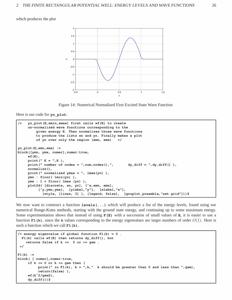
2 THE FINITE RECTANGULAR POTENTIAL WELL: ENERGY LEVELS AND WAVE FUNCTIONS 26
which produces the plot
-2
-1.5
-1
-0.5
0
0.5
1
1.5
2
-0.5 0 0.5 1 1.5
y
x
Figure 14: Numerical Normalized First Excited State Wave Function
Here is our code foryn_plot :
/ * yn_plot(E,xmin,xmax) first calls wf(E) to createun-normalized wave functions corresponding to the
given energy E. Then normalizes those wave functionsto produce the lists xn and yn. Finally makes a plotof yn over only the region (xmn, xmx) * /
yn_plot(E,xmn,xmx) :=block([ymn, ymx, numer],numer:true,
wf(E),print(" E = ",E ),print(" number of nodes = ",num_nodes(),", dy_diff = ",dy_d iff() ),normalize(),print(" normalized ymax = ", lmax(yn) ),ymn : floor( lmin(yn) ),ymx : 1 + floor( lmax (yn) ),plot2d( [discrete, xn, yn], [’x,xmn, xmx],
[’y,ymn,ymx], [ylabel,"y"], [xlabel,"x"],[style, [lines, 3] ], [legend, false], [gnuplot_preamble, "set grid"]))$
We now want to construct a functionlevels(...) which will produce a list of the energy levels, found using ournumerical Runge-Kutta methods, starting with the ground state energy, and continuing up to some maximum energy.Some experimentation shows that instead of usingF(E) with a succession of small values ofE, it is easier to use afunction F1(k) , since thek values corresponding to the energy eigenvalues are larger numbers of orderO(1). Here issuch a function which we callF1(k) .
/ * energy eigenvalue if global function F1(k) = 0 .F1(k) calls wf(E) then returns dy_diff(), but
returns false if k <= 0 or >= gam .
* /
F1(k) :=block( [ numer],numer:true,
if k <= 0 or k >= gam then (print(" in F1(k), k = ",k," k should be greater than 0 and less t han ",gam),return(false) ),
wf(kˆ2/gam2),dy_diff())$

2 THE FINITE RECTANGULAR POTENTIAL WELL: ENERGY LEVELS AND WAVE FUNCTIONS 27
Here is an example of use ofF1(k) to find the ground state energy:
(%i23) F1(2.9);(%o23) 34.29503(%i24) F1(3.05);(%o24) -49.882755(%i25) [ka,kb] : bracket(F1,2.9,0.05,0.02);(%o25) [3.0125,3.025](%i26) k0 : find_root(F1,ka,kb);(%o26) 3.0206914(%i27) E0 : ktoE(k0);(%o27) 0.00364983(%i28) wf(E0);(%o28) done(%i29) dy_diff();(%o29) -1.49739046E-13(%i30) num_nodes();(%o30) 0
which reveals a zero node wave function with a very small value of dy_diff() , a signal of a good wave function.
We can make a crude plot ofF1(k) versusk
(%i31) kL : makelist(k,k,1,49,0.5)$(%i32) F1L : map(F1, kL)$(%i33) time(%);(%o33) [6.23](%i34) plot2d([discrete,kL,F1L],[xlabel,"k"],[ylabel ,"F1(k)"])$
which produces the plot
-500
0
500
1000
1500
2000
0 5 10 15 20 25 30 35 40 45 50
F1(
k)
k
Figure 15: Crude Plot of F1(k) versus k
Let’s useF1(k) to look at the region2.8 <= k <= 3.3 :
(%i315 kL : makelist(k,k,2.8,3.3,0.05)$(%i36) F1L : map(F1, kL)$(%i37) plot2d([discrete,kL,F1L],[xlabel,"k"],[ylabel ,"F1(k)"])$

2 THE FINITE RECTANGULAR POTENTIAL WELL: ENERGY LEVELS AND WAVE FUNCTIONS 28
which produces the plot
-50
0
50
100
150
200
250
2.75 2.8 2.85 2.9 2.95 3 3.05 3.1 3.15 3.2 3.25 3.3
F1(
k)
k
Figure 16: F1(k) Zoom
Placing the cursor on theF1 = 0 intersections shows roots at roughlyk = 3.01 andk = 3.06 . The first root is closeto the valid ground state case as shown above. We can usebracket with F1(k) to refine the second root.
(%i38) [ka,kb] : bracket(F1,3.03,0.01,0.005);(%o38) [3.0775,3.08](%i39) kv : find_root(F1,ka,kb);(%o39) 3.0799546(%i40) Ev : ktoE(kv);(%o40) 0.00379445(%i41) wf(Ev);(%o41) done(%i42) num_nodes();(%o42) 0(%i43) dy_diff();(%o43) -1.60000886E+16
The large value ofdy_diff() shows that this second, slightly larger root, is an un-physical solution. Since we alreadyhave a valid zero node solution at the lower energy, there cannot be a second zero node solution at another, higher, energy.This pattern persists, with the physical root being smaller, and the un-physical root being slightly larger. This patternprovides the rationale for our code forlevels(...) . Once we have found a solution with a given number of nodes,we reject all solutions with higher energy but the same number of nodes. The unphysical roots correspond to a suddenchange in which (left or right) integration function has thelarger slope magnitude at the matching point.
Here is our code forlevels(kmin,kmax,dk, kacc ) .
/ * levels(kmin,kmax,dk, kacc ) returns a list [Ea, Eb,...] of e nergy levels withincreasingly larger number of nodes in energy range (Emin, E max)according to Emin = kminˆ2/gamˆ2, and Emax = kmaxˆ2/gamˆ2.uses F1(k) (inside bracket) to find roots, and calls wf(E), n um_nodes() and
dy_diff() for each root found,Uses bracket and find_root.The arguments (dk, kacc) are used to call bracket, and do not d escribe
the accuracy of the energy levels found.Once a good energy e.v. is found we look for the region of
energies with one more node and search there.Includes an interactive continue or stop input.Searching for the k eigenvalues via F1(k) is easier than sear ching
directly for the E eigenvalues via F(E) for the case gam = 50 wh ich weconsider in our examples.
* /

2 THE FINITE RECTANGULAR POTENTIAL WELL: ENERGY LEVELS AND WAVE FUNCTIONS 29
levels(kmin,kmax,dk, kacc ) :=block([ k,knext, kroot,eroot, eL, ka, kb, nn, nlast : -1, r, n umer], numer:true,
k : kmin,eL : [ ], / * list eL will hold energy eigenvalues found * /do (
if k > kmax then return(), / * exit do loop * /print("---------------- levels -------------------"),print(" nlast = ", nlast),print(" kstart = ", k," dk = ", dk ),[ka, kb] : bracket(F1,k, dk, kacc),print(" ka = ",ka," kb = ",kb),if float(ka) = 0.0 then (
print(" can’t find bracket interval "),print(" k = ",k),return() ),
kroot : find_root(F1, ka, kb),print(" kroot = ", kroot),eroot : krootˆ2/gam2,print(" eroot = ", eroot),wf(eroot),nn : num_nodes(),print(" number of nodes = ", nn),print(" dy_diff at x = 1 is ", dy_diff() ),eL : cons(eroot, eL),nlast : nn,r : read (" input c; or s; "),if string(r) = "s" then return(), / * exit do loop * /
/ * search for a k value greater than kb which producesa wave function with nn + 1 nodes * /
knext : kb + dk,do (
wf(knextˆ2/gam2),if num_nodes() > nlast then (
k : knext,return() )
else knext : knext + dk)),
reverse(eL) )$
Here is an example of usinglevels . To continue to the next energy eigenvalue, one entersc; at the prompt (for“continue”). Actually, any letter excepts; will cause the program to continue.
(%i44) EL : levels(1,8,0.05,0.02);---------------- levels -------------------
nlast = -1kstart = 1 dk = 0.05ka = 3.0125 kb = 3.025kroot = 3.0206914eroot = 0.00364983number of nodes = 0dy_diff at x = 1 is -2.49565076E-14input c; or s;
c;---------------- levels -------------------
nlast = 0kstart = 3.125 dk = 0.05ka = 6.0375 kb = 6.05kroot = 6.040956eroot = 0.0145973number of nodes = 1dy_diff at x = 1 is 2.18273877E-13input c; or s;
c;

2 THE FINITE RECTANGULAR POTENTIAL WELL: ENERGY LEVELS AND WAVE FUNCTIONS 30
---------------- levels -------------------nlast = 1kstart = 6.2 dk = 0.05ka = 9.05 kb = 9.0625kroot = 9.0603555eroot = 0.032836number of nodes = 2dy_diff at x = 1 is 7.10273285E-14input c; or s;
c;(%o44) [0.00364983,0.0145973,0.032836]
We can then useyn_plot(E,xmin,xmax) to both construct the listsxn andyn of the normalized wave function andmake a plot. We can also usemakelist to construct one listxyn , say, which combines the listsxn andyn into one. Inthe following, we do not show the plots produced by the calls to yn_plot .
(%i45) yn_plot(EL[1],-0.5,1.5)$E = 0.00364983number of nodes = 0 , dy_diff = -2.49565076E-14AA = 6652.6824x_mean = 0.5delx = 0.18802normalized ymax = 1.3867012
(%i46) xyn0 : makelist([xn[j],yn[j]],j,1,length(xn))$(%i47) fll(xyn0);(%o47) [[-0.5,0.0],[1.5,0.0],201]
We continue in this manner with the first excited state and thesecond excited state.
(%i48) yn_plot(EL[2],-0.5,1.5)$E = 0.0145973number of nodes = 1 , dy_diff = -2.05936658E-12AA = 1278.4068x_mean = 0.5delx = 0.276562normalized ymax = 1.3865517
(%i49) xyn1 : makelist([xn[j],yn[j]],j,1,length(xn))$(%i50) yn_plot(EL[3],-0.5,1.5)$
E = 0.032836number of nodes = 2 , dy_diff = -2.00652203E-12AA = 365.3835x_mean = 0.5delx = 0.290108normalized ymax = 1.385693
(%i51) xyn2 : makelist([xn[j],yn[j]],j,1,length(xn))$
We can then combine the plots for the wave functions of these three lowest lying states.
(%i52) plot2d([[discrete,xyn0],[discrete,xyn1],[disc rete,xyn2]],[xlabel,"x"],[ylabel,"y"],[style,[lines,2]],
[legend,"E0","E1","E2"])$

2 THE FINITE RECTANGULAR POTENTIAL WELL: ENERGY LEVELS AND WAVE FUNCTIONS 31
which produces the plot
-1.5
-1
-0.5
0
0.5
1
1.5
-0.5 0 0.5 1 1.5
y
x
E0E1E2
Figure 17: Finite Well: Lowest Three Energy Level Wave Functions
Just for practice, we can write these three wave functions toa file in the local folder, and then restart Maxima, read in thefile contents, and make a plot based on the file contents. We have discussed some details of such read and write actionswithin Maxima in Chapter 2 of Maxima by Example.
The simplest approach is to usesave(filePath,a1,a2,a3,...) , where objectsa1, a2, etc are object names boundto quantities known to Maxima. The names and the objects bound to the names are stored in Lisp language format in thefile requested (which is created if it does not yet exist, and overwritten if it already exists). You can, of course, open thatfile with a text editor to see the contents, written in Lisp.
One can useload to load in that file into a new Maxima session, and the names andobjects will then be available for usein your new Maxima session. If you don’t remember the names you used in your previous session, you can usevalues;
to generate a list of currently known object names.
(%i53) E0 : EL[1];(%o53) 0.00364983(%i54) E1 : EL[2];(%o54) 0.0145973(%i55) E2 : EL[3];(%o55) 0.032836(%i56) save("c:/k3/fw1.dat",E0,xyn0,E1,xyn1,E2,xyn2) ;(%o56) "c:/k3/fw1.dat"
If we look at the top of the filec:/k3/fw1.dat with a text editor (such asNotepad++) we see:
;;; - * - Mode: LISP; package:maxima; syntax:common-lisp; - * -(in-package :maxima)(DSKSETQ |$e0| 0.0036498306077588829)(ADD2LNC ’|$e0| $VALUES)(DSKSETQ $XYN0
’((MLIST SIMP) ((MLIST SIMP) -0.5 0.0)((MLIST SIMP) -0.48999999999999999 1.2769296242295217E -12)((MLIST SIMP) -0.47999999999999998 2.8785287263561221E -12)((MLIST SIMP) -0.46999999999999997 5.2117339500682875E -12)((MLIST SIMP) -0.46000000000000002 8.8694267352155839E -12)((MLIST SIMP) -0.45000000000000001 1.4781088055950433E -11)
etc., etc.
We now restart Maxima and load incp3.mac , FW.mac, and the data file created usingsave above.

2 THE FINITE RECTANGULAR POTENTIAL WELL: ENERGY LEVELS AND WAVE FUNCTIONS 32
(%i1) load(cp3);(%o1) "c:/k3/cp3.mac"(%i2) load(FW);
gam = 50 gam2 = 2500h = 0.01 , xdecay = 0.5 , ypleft = 1.0E-8 ypright = 1.0E-8
(%o2) "c:/k3/FW.mac"(%i3) load("c:/k3/fw1.dat");(%o3) "c:/k3/fw1.dat"(%i4) values;(%o4) [mydate,_binfo%,N,h,gam,gam2,xdecay,ypleft,ypr ight,E0,xyn0,E1,xyn1,E2,xyn2](%i5) E0;(%o5) 0.00364983(%i6) E1;(%o6) 0.0145973(%i7) E2;(%o7) 0.032836(%i8) fll(xyn0);(%o8) [[-0.5,0.0],[1.5,0.0],201](%i9) head(xyn0);(%o9) [[-0.5,0.0],[-0.49,1.27692962E-12],[-0.48,2.87 852873E-12],
[-0.47,5.21173395E-12],[-0.46,8.86942674E-12],[-0.4 5,1.47810881E-11]](%i10) plot2d([[discrete,xyn0],[discrete,xyn1],[disc rete,xyn2]],
[xlabel,"x"],[ylabel,"y"],[style,[lines,2]],[legend,"E0","E1","E2"])$
and we get the same plot as above.
2.2.2 Numerical Energies and Wave Functions using R
We use our homemademyrk4 routine for the Runge-Kutta integration. When the fileFW.R is loaded, a number of globalparameters are defined. The top the the fileFW.Rhas the lines:
## FW.R uses Runge-Kutta for finite well.
## dimensionless units## V = 1 for x < 0 and x > 1## V = 0 for 0 < x < 1## y’’(x) + gam2 * (E - V(x)) * y(x) = 0## gam2 = gamˆ2 = 2500## gam = 50 = sqrt(2 * m* Lˆ2 * V0/ hbarˆ2)
## initial global parameters:
N = 100h = 0.01gam = 50gam2 = gamˆ2xdecay = 0.5 ## start yL1 integration at x = -xdecay
## start yR integration at x = 1 + xdecayypleft = 1e-8ypright = 1e-8debug = FALSEwfdebug = FALSEcat (" gam = ",gam, " gam2 = ", gam2,"\n")cat (" h = ", h, ", xdecay = ", xdecay, ",ypleft = ", ypleft," ypr ight = ",ypright,"\n")
We integrate from a pointx = -xdecay chosen so that we can assumey(-xdecay) = 0 to the pointx = 0 , thusdefining a grid vectorxL1 of integration points, a vectoryL1 of values ofy(x) at these grid points, and a vectorypL1 ofvalues ofy′(x) at these grid points whereV = 1.
We assume an arbitrary small valueypleft for the first derivativey′ at this starting point. The resulting wave function,the solution of a homogeneous equation, can be later normalized, which will, in effect, amount to choosing the correct

2 THE FINITE RECTANGULAR POTENTIAL WELL: ENERGY LEVELS AND WAVE FUNCTIONS 33
initial first derivative at the left starting point.
The final value ofy andy′ thus generated become the initial values ofy andy′ for integration through the region whereV = 0, 0 ≤ x ≤ 1, thus generating a grid vectorxL2 of integration points, a vectoryL2 of values ofy(x) at these gridpoints, and a vectorypL2 of values ofy′(x) at these grid points whereV = 0.
The integration in the regionx > 1 is done by starting at a locationx = 1 + xdecay where we can assumey = 0and we again assign an arbitrary (but negative) first derivative -ypright . We then integrate toward smaller values ofxuntil we reachx = 1. Since we are hence integrating in the direction in which thephysical solution is growing, we avoidintegration instability problems produced by small roundoff and integration algorithm errors.
We then multiply the vectorsyL1 , ypL1 , yL2 , andypL2 by a factor which assures us that the final value ofy(x) producedby the independent rightward and leftward integrations agree at the matching pointx = 1. The value ofy(x) can be madeto agree at the matching point for any energyE. However, the resulting wave function values will still be discontinuousbecause the first derivatives will not agree at the matching point.
The crucial step, then, is to design a functionF (E), say, that is zero (to within numerical errors) when the derivativesagree at the matching point. We can then look for the locations of sign changes inF (E) to locate the energy eigenvalues.
The first step needed, in order to be able to design such a function F(E) , is to design a functionwf(E) which uses RungeKutta methods to find a un-normalized wave function corresponding to a given total energyE. Here is our code for sucha wave function integrator, as listed inFW.R.
## wf(E) creates ** un-normalized ** numerical wave functions## using Runge-Kutta routine myrk4.## The wave functions are stored in global vectors## xL1, yL1,ypL1, xL2, yL2, ypL2, xR, yR, ypR .## Program also defines ** global ** nleft, nright, ncenter.## the global xL1 grid extends from -xdecay to 0 and## the global xL2 grid extends from 0 to 1 and## the global xR grid extends from 1 to 1 + xdecay
wf = function (E) {if ( (E < 0) | (E > 1) ) {
cat (" need 0 < E < 1 \n")return(false) }
ncenter = Nif ( round(ncenter) != ncenter) {
cat (" ncenter = ",ncenter," is not an integer \n")return(false) }
nleft = round(xdecay/h)nright = nleftif (wfdebug) cat (" nleft = ",nleft," ncenter = ",ncenter," n right = ",nright, "\n")glr = gam2 * (E - 1) ## g(x) for x < 0 and x > 1gc = gam2* E ## g(x) for 0 < x < 1if (wfdebug) cat (" glr = ",glr," gc = ", gc, "\n")## construct xl1, yl1, and ypl1 for -xdecay < x < 0derivs.decay = function (x,y) { c (y[2], - glr * y[1]) }xl1 = seq (- xdecay, 0, h)outL = myrk4( c(0,ypleft), xl1, derivs.decay)yl1 = outL[[1]]ypl1 = outL[[2]]## construct xl2, yl2, and ypl2 for 0 < x < 1derivs01 = function (x,y) { c (y[2], - gc * y[1]) }xl2 = seq(0, 1, h)outL = myrk4( c(last(yl1), last(ypl1)), xl2, derivs01)yl2 = outL[[1]]ypl2 = outL[[2]]

2 THE FINITE RECTANGULAR POTENTIAL WELL: ENERGY LEVELS AND WAVE FUNCTIONS 34
## construct xr, yr, and ypr for 1 < x < 1 + xdecayxr = seq( 1 + xdecay, 1, -h)outL = myrk4( c(0, -ypright), xr, derivs.decay)yr = outL[[1]]ypr = outL[[2]]xr = rev(xr)yr = rev(yr)ypr = rev(ypr)if (wfdebug) cat (" yr(1) = ", yr[1], "\n" )fac = yr[1] / last(yl2)if (wfdebug) cat (" fac = ",fac, "\n")yl1 = fac * yl1ypl1 = fac * ypl1yl2 = fac * yl2ypl2 = fac * ypl2## make global xL1,xL2,xR,yL1,yL2,yR,ypL1,ypL2,ypRxL1 <<- xl1xL2 <<- xl2xR <<- xryL1 <<- yl1yL2 <<- yl2yR <<- yrypL1 <<- ypl1ypL2 <<- ypl2ypR <<- ypr }
The second step needed to designF(E) is to create a functiondy_diff() which returns a normalized difference of thefirst derivativesy′L(x) − y′R(x) evaluated at the matching pointx = 1. We return this difference divided by the value ofy(x = 1).
## dy_diff() uses global ypL2, ypR, and yR,## returns a normalized difference of derivatives## (yL’(1) - yR’(1)/ yR(1)
dy_diff = function () {dy_left = last(ypL2)dy_right = ypR[1](dy_left - dy_right)/abs( yR[1] ) }
For example,
> wf(0.5)> dy_diff()[1] 35.0717> last(ypL2)[1] -0.00190471> ypR[1][1] -0.237432> yR[1][1] 0.00671558
Here is our code forF(E) :
## energy eigenvalue if global function F(E) = 0 .## F(E) calls wf(E) then returns dy_diff(), but## returns FALSE if E < 0 or > 1 .F = function (E) {
if (E < 0 | E > 1) {cat (" in F(E), E = ",E," should be between 0 and 1 \n ")return(FALSE) }
wf(E)dy_diff() }

2 THE FINITE RECTANGULAR POTENTIAL WELL: ENERGY LEVELS AND WAVE FUNCTIONS 35
Here is an example of usingF(E) to produce a rough graphical survey of the possibilities:
> EL = seq(0.1,0.9,0.01)> FL = sapply(EL, F)> fll(FL)
82.3613 17.2303 81> plot(EL, FL, type = "l", lwd = 2, col = "blue", xlab = "E",ylab = "F(E)" )> mygrid()
which produces the plot
0.2 0.4 0.6 0.8
−20
00
200
400
600
800
E
F(E
)
Figure 18: Crude Plot of F(E)
We can useF(E) to search for energy eigenvalue candidates. We do this with afunctionbracket(func,x,dx,xacc)
which attempts to return two values ofx at whichfunc has the opposite sign.
## bracket is a modified version of bracket_basic, designed to work with## the functions F(E) or F1(k) which can return FALSE.## bracket looks for a sign change in func,## starting with xx, and increasing xx by dxx each step.## If sign change is found, then we back up to the previous xx## and search with new dxx value one half of the previous value .## normally returns [ea,eb], but if can’t find change in sign ,## then returns [0,0], and if func returns FALSE, then## bracket returns FALSE.
bracket = function (func,xx,dxx,xacc) {x = xxdx = dxxit = 0itmax = 1000anerror = FALSEanerror2 = FALSE
repeat {it = it + 1if (it > itmax) {
cat (" can’t find change in sign \n")

2 THE FINITE RECTANGULAR POTENTIAL WELL: ENERGY LEVELS AND WAVE FUNCTIONS 36
anerror = TRUEbreak}
x1 = xx2 = x + dxif ( debug ) cat (" it = ",it," x1 = ",x1," x2 = ",x2," dx = ", dx, "\ n")f1 = func(x1)if ( f1 == FALSE) {
cat (" in bracket, f1 = FALSE , x1 = ",x1, " dx = ", dx, " \n ")anerror2 = TRUEbreak }
f2 = func(x2)if ( f2 == FALSE) {
cat (" in bracket, f2 = FALSE , x2 = ",x2, " dx = ", dx, " \n ")anerror2 = TRUE
break }if ( f1 * f2 < 0 ) {
if ( abs(dx) < xacc ) breakx = x - dxdx = dx/2 } else x = x2 }
if (anerror) c(0,0) else if (anerror2) FALSE else c(x1,x2) }
Here is an example of usingbracket with the functionF(E) . This example produces the zero node ground state case,and we plot the un-normalized wave function pieces producedby wf(E) .
> out = bracket(F,0.0005,0.0001,0.00005)> out[1] 0.003625 0.003650> e = uniroot(F,out, tol = 1e-16)$root> e[1] 0.00364983> wf(e)> plot(0, type = "n", xlim = c(min(xL1), max(xR)), ylim = c(0, max(yL2)),+ xlab = "x", ylab = "y" )> lines (xL1, yL1, lwd = 3, col = "blue")> lines (xL2, yL2, lwd = 3, col = "red")> lines (xR, yR, lwd = 3, col = "green")> mygrid()
which produces a plot of the un-normalized ground state wavefunction with zero nodes.
−0.5 0.0 0.5 1.0 1.5
020
4060
8010
0
x
y
Figure 19: Numerical Un-normalized Ground State Wave Function
We can check the normalized difference in slopes at the matching point for the solution produced bywf(E) :
> dy_diff()[1] -3.42736e-12

2 THE FINITE RECTANGULAR POTENTIAL WELL: ENERGY LEVELS AND WAVE FUNCTIONS 37
We can check the number of nodes with the functionnum_nodes() .
num_nodes = function () {n = 0for ( j in 1 : (length(yL2) - 1) ) { if (yL2[ j ] * yL2[ j + 1 ] < 0) n = n + 1 }n }
For the numerical ground state solution generated above bywf(E) we get:
> num_nodes()[1] 0
A functionnormalize() uses the current wave function pieces produced bywf(E) and uses our Simpson’s rule functionsimp to produce global normalized wave function (vectors)xn andyn . We use the functionrest defined incp3.R innormalize() .
Before we usenormalize() , let’s show interactively the route we follow in the beginning of normalize() :
> xn = c (xL1, c ( rest(xL2), rest(xR) ) )> fll(xn)
-0.5 1.5 201> yn = c (yL1, c ( rest(yL2), rest(yR) ) )> fll(yn)
0 0 201> head(xn)[1] -0.50 -0.49 -0.48 -0.47 -0.46 -0.45> head(yn)[1] 0.00000e+00 1.04151e-10 2.34784e-10 4.25090e-10 7.23 426e-10 1.20560e-09> simp(xn,ynˆ2)[1] 6652.68
Here we callnormalize() , and then check the normalization interactively using Simpson’s rulesimp .
> normalize()AA = 6652.68x_mean = 0.5delx = 0.18802
> simp(xn,ynˆ2)[1] 1
Here is the code fornormalize() .
## normalize() uses the current global xL1,yL1, xL2,yL2, xR , yR and## the utility functions rest and simp to define global## xn and yn, with the latter being normalized.
normalize = function () {
xn = c (xL1, c ( rest(xL2), rest(xR) ) )yn = c (yL1, c ( rest(yL2), rest(yR) ) )## we need xn to have odd number of elements to use simpif ( is.even ( length (xn) ) ) {
xn = rest (xn)yn = rest (yn) }
AA = simp(xn,ynˆ2)cat ( " AA = ",AA, "\n" )yn = yn/sqrt(AA)x_mean = simp(xn, xn * ynˆ2)cat (" x_mean = ", x_mean, "\n" )x2_mean = simp(xn, xnˆ2 * ynˆ2)delx2 = x2_mean - x_meanˆ2 ## this should be positive!delx = sqrt(delx2)cat (" delx = ", delx, "\n" )xn <<- xnyn <<- yn }

2 THE FINITE RECTANGULAR POTENTIAL WELL: ENERGY LEVELS AND WAVE FUNCTIONS 38
After usingnormalize() , one can plot the normlized wave function (the current vectors xn andyn ) using the functionyn_plot_current() :
> yn_plot_current()ymax = 1.3867
which produces the plot
−0.5 0.0 0.5 1.0 1.5
0.0
0.5
1.0
1.5
2.0
x
y
Figure 20: Numerical Normalized Ground State Wave Function
The functionyn_plot_current() uses the current global vectorsxn andyn created bynormalize() .
## yn_plot_current() uses the currently defined normalize d set (xn,yn)yn_plot_current = function () {
ymn = floor( min(yn) )ymx = 1 + floor( max (yn) )cat (" ymax = ", max(yn), "\n" )plot(xn, yn, type = "l", lwd = 3, col = "blue", ylim = c(ymn, ymx ),
xlab = "x", ylab = "y", tck = 1) }
The more versatile functionyn_plot(E,xmin,xmax) does three tasks in succession, first callingwf(E) to create theun-normalized wave function pieces, then callingnormalize() to create the normalized wave function vectors in theform of xn andyn , and finally making a plot of the normalized wave function, using xmin andxmax to control the display.
Here is an example dealing with the first excited (one node) state.
> out = bracket(F,0.01,0.005,0.001)> out[1] 0.014375 0.015000> e = uniroot(F,out, tol = 1e-16)$root> e[1] 0.0145973> yn_plot(e,-0.5,1.6)
E = 0.0145973number of nodes = 1 , dy_diff = 1.61333e-13AA = 1278.41x_mean = 0.5delx = 0.276562normalized ymax = 1.38655

2 THE FINITE RECTANGULAR POTENTIAL WELL: ENERGY LEVELS AND WAVE FUNCTIONS 39
which produces the plot
−0.5 0.0 0.5 1.0 1.5
−2
−1
01
2
x
y
Figure 21: Numerical Normalized First Excited State Wave Function
Here is our code foryn_plot :
## yn_plot(E,xmin,xmax) first calls wf(E) to create## un-normalized wave functions corresponding to the## given energy E. Then normalizes those wave functions## to produce the vectors xn and yn. Finally makes a plot## of yn over only the region (xmn, xmx)
yn_plot = function (E,xmn,xmx) {wf(E)cat (" E = ",E, "\n" )cat (" number of nodes = ",num_nodes(),", dy_diff = ",dy_dif f(), "\n" )normalize()cat (" normalized ymax = ", max(yn), "\n" )ymn = floor( min(yn) )ymx = 1 + floor( max (yn) )plot(xn, yn, type = "l", lwd = 3, col = "blue", xlim = c(xmn,xmx ), ylim = c(ymn, ymx),
xlab = "x", ylab = "y", tck = 1) }
We now want to construct a functionlevels(...) which will produce a vector of the energy levels, found usingournumerical Runge-Kutta methods, starting with the ground state energy, and continuing up to some maximum energy.Some experimentation shows that instead of usingF(E) with a succession of small values ofE, it is easier to use afunction F1(k) , since thek values corresponding to the energy eigenvalues are larger numbers of orderO(1). Here issuch a function, which we callF1(k) .
## F1(k): energy eigenvalue if global function F1(k) = 0 .## F1(k) calls wf(E) then returns dy_diff(), but## returns false if k <= 0 or k >= gam.F1 = function (k) {
if (k <= 0 | k >= gam) {cat (" in F1(k), k = ",k," k should be greater than 0 and less tha n ",gam, "\n")return(FALSE) }
wf(kˆ2/gam2)dy_diff() }

2 THE FINITE RECTANGULAR POTENTIAL WELL: ENERGY LEVELS AND WAVE FUNCTIONS 40
Here is an example of use ofF1(k) to find the ground state energy:
> F1(2.9)[1] 34.295> F1(3.05)[1] -49.8828> out = bracket(F1,2.9,0.05,0.02)> out[1] 3.0125 3.0250> k0 = uniroot(F1, out, tol = 1e-16)$root> k0[1] 3.02069> E0 = ktoE(k0)> E0[1] 0.00364983> wf(E0)> dy_diff()[1] 3.41072e-13> num_nodes()[1] 0
which reveals a zero node wave function with a very small value of dy_diff() , a signal of a good wave function.
We can make a crude plot ofF1(k) versusk
> kL = seq(1,49,by=0.5)> head(kL)[1] 1.0 1.5 2.0 2.5 3.0 3.5> F1L = sapply (kL, F1)> head (F1L)[1] 50.6042 50.0387 48.9460 46.2163 13.2072 57.5400> plot(kL, F1L, type = "l", lwd = 2,col = "blue",xlab = "k",yla b = "F1(k)")> mygrid()
which produces the plot
0 10 20 30 40 50
050
010
0015
00
k
F1(
k)
Figure 22: Crude Plot of F1(k) versus k

2 THE FINITE RECTANGULAR POTENTIAL WELL: ENERGY LEVELS AND WAVE FUNCTIONS 41
Let’s useF1(k) to look at the region2.8 <= k <= 3.3 :
> kL = seq (2.8, 3.3, by = 0.05)> head(kL)[1] 2.80 2.85 2.90 2.95 3.00 3.05> F1L = sapply( kL, F1)> head(F1L)[1] 40.3843 37.9920 34.2950 27.7891 13.2072 -49.8828> plot(kL, F1L, type = "l", lwd = 2,col = "blue",xlab = "k",yla b = "F1(k)")> mygrid()
which produces the plot
2.8 2.9 3.0 3.1 3.2 3.3
−50
050
100
150
200
k
F1(
k)
Figure 23: F1(k) Zoom
This zoom plot shows roots at roughlyk = 3.01 andk = 3.06 . The first root is close to the valid ground state case asshown above. We can usebracket with F1(k) to refine the second root.
> out = bracket(F1,3.03,0.01,0.005)> out[1] 3.0775 3.0800> kv = uniroot(F1, out, tol = 1e-16)$root> kv[1] 3.07995> Ev = ktoE(kv)> Ev[1] 0.00379445> wf(Ev)> num_nodes()[1] 0> dy_diff()[1] -2.64829e+15
The large value ofdy_diff() shows that this second, slightly larger root, is an un-physical solution. Since we alreadyhave a valid zero node solution at the lower energy, there cannot be a second zero node solution at another, higher, energy.This pattern persists, with the physical root being smaller, and the un-physical root being slightly larger. This patternprovides the rationale for our code forlevels(...) . Once we have found a solution with a given number of nodes,we reject all solutions with higher energy but the same number of nodes. The unphysical roots correspond to a suddenchange in which (left or right) integration function has thelarger slope magnitude at the matching point.

2 THE FINITE RECTANGULAR POTENTIAL WELL: ENERGY LEVELS AND WAVE FUNCTIONS 42
Here is an example of usinglevels .
> EL = levels(1,8,0.05,0.02)---------------- levels -------------------
nlast = -1kstart = 1 dk = 0.05ka = 3.0125 kb = 3.025kroot = 3.02069eroot = 0.00364983number of nodes = 0dy_diff at x = 1 is 3.41072e-13input c or sc
---------------- levels -------------------nlast = 0kstart = 3.125 dk = 0.05ka = 6.0375 kb = 6.05kroot = 6.04096eroot = 0.0145973number of nodes = 1dy_diff at x = 1 is 1.61333e-13input c or sc
---------------- levels -------------------nlast = 1kstart = 6.2 dk = 0.05ka = 9.05 kb = 9.0625kroot = 9.06036eroot = 0.032836number of nodes = 2dy_diff at x = 1 is -1.36136e-13input c or sc
> EL[1] 0.00364983 0.01459726 0.03283602
We can then useyn_plot(E,xmin,xmax) to both construct the vectorsxn andyn of the normalized wave functionand make a plot. We save the normalized wave functions by assignment statements such asxn0 = xn , andyn0 = yn ,before another call toyn_plot defines the wave functions corresponding to a different energy. In the following, we donot show the plots produced by the calls toyn_plot .
> yn_plot(EL[1],-0.5,1.5)E = 0.00364983number of nodes = 0 , dy_diff = 3.41072e-13AA = 6652.68x_mean = 0.5delx = 0.18802normalized ymax = 1.3867
> xn0 = xn> fll(xn0)
-0.5 1.5 201> yn0 = yn> fll(yn)
0 0 201
We continue in this manner with the first excited state and thesecond excited state.
> yn_plot(EL[2],-0.5,1.5)E = 0.0145973number of nodes = 1 , dy_diff = 1.61333e-13AA = 1278.41x_mean = 0.5delx = 0.276562normalized ymax = 1.38655
> xn1 = xn> fll(xn1)
-0.5 1.5 201> yn1 = yn> fll(yn1)
0 0 201

2 THE FINITE RECTANGULAR POTENTIAL WELL: ENERGY LEVELS AND WAVE FUNCTIONS 43
> yn_plot(EL[3],-0.5,1.5)E = 0.032836number of nodes = 2 , dy_diff = -1.36136e-13AA = 365.384x_mean = 0.5delx = 0.290108normalized ymax = 1.38569
> xn2 = xn> yn2 = yn
We can then combine the plots for the wave functions of these three lowest lying states.
> plot(0,type = "n",xlim = c(-0.5,1.5),ylim = c(-1.5,1.5), xlab="x",ylab="y")> lines(xn0,yn0,lwd=2,col="blue")> lines(xn1,yn1,lwd=2,col="red")> lines(xn2,yn2,lwd=2,col="green")> mygrid()> legend("bottomright",col = c("blue","red","green"),+ legend = c("E0", "E1", "E2"), lwd=2,cex=1.5)
which produces the plot
−0.5 0.0 0.5 1.0 1.5
−1.
5−
1.0
−0.
50.
00.
51.
01.
5
x
y
E0E1E2
Figure 24: Finite Well: Lowest Three Energy Level Wave Functions
Just for practice, we can write these three wave functions toa file in the local folder, and then restartR, read in the filecontents, and make a plot based on the file contents.
The simplest approach is to usesave(filePath,a1,a2,a3,...) , where objectsa1, a2, etc are object names boundto quantities known to R. The names and the objects bound to the names are stored in a binary file format in the filerequested (which is created if it does not yet exist, and overwritten if it already exists).
One can useload to load in that file into a new session, and the names and objects will then be available for use inyour new Maxima session. In the following, we first save the wave function files toxy.rda . We then userm to removeknowledge of those objects from the current session. We thenuseload to recover knowledge of those objects, which canthen be used as before, for example to make plots and make calculations.
> save(xn0,yn0,xn1,yn1,xn2,yn2, file = "xy.rda")> rm(xn0,yn0,xn1,yn1,xn2,yn2)

2 THE FINITE RECTANGULAR POTENTIAL WELL: ENERGY LEVELS AND WAVE FUNCTIONS 44
> fll(xn0)Error in fll(xn0) : object ’xn0’ not found> load("xy.rda")> fll(xn0)
-0.5 1.5 201
For example, we can remake the plot of all three wave functions
> plot(0,type = "n",xlim = c(-0.5,1.5),ylim = c(-1.5,1.5), xlab="x",ylab="y")> lines(xn0,yn0,lwd=2,col="blue")> lines(xn1,yn1,lwd=2,col="red")> lines(xn2,yn2,lwd=2,col="green")> mygrid()> legend("bottomright",col = c("blue","red","green"),+ legend = c("E0", "E1", "E2"), lwd=2,cex=1.5)
and we get the same plot as above.
Here is the code forlevels :
## levels(kmin,kmax,dk, kacc ) returns a vector c( Ea, Eb,.. .) of energy levels with## increasingly larger number of nodes in energy range (Emin , Emax)## according to Emin = kminˆ2/gamˆ2, and Emax = kmaxˆ2/gamˆ2 .## uses F1(k) (inside bracket) to find roots, and calls wf(E) , num_nodes() and## dy_diff() for each root found,## Uses bracket and uniroot.## The arguments (dk, kacc) are used to call bracket, and do no t describe## the accuracy of the energy levels found.## Once a good energy e.v. is found we look for the region of## energies with one more node and search there.## Code has interactive continue or stop.## Searching for the k eigenvalues via F1(k) is easier than se arching## directly for the E eigenvalues via F(E) for the case gam = 50 we## consider in this example.levels = function (kmin,kmax,dk, kacc ) {
rmax = 20eL = rep(NA, rmax) ## vector eL will hold energy eigenvalues f oundk = kminnlast = -1j = 1repeat {
if (k > kmax | j > rmax) break ## exit do loopcat ("---------------- levels -------------------\n")cat (" nlast = ", nlast,"\n")cat (" kstart = ", k," dk = ", dk, "\n" )out = bracket(F1,k, dk, kacc)cat (" ka = ",out[1]," kb = ",out[2],"\n")if (out[1] == 0) {
cat (" can’t find bracket interval \n")cat (" k = ",k, "\n")break }
kroot = uniroot(F1, out, tol = 1e-16)$rootcat (" kroot = ", kroot, "\n")eroot = krootˆ2/gam2cat (" eroot = ", eroot, "\n")wf(eroot)nn = num_nodes()cat (" number of nodes = ", nn, "\n")cat (" dy_diff at x = 1 is ", dy_diff(), "\n" )eL[ j ] = erootnlast = nnj = j + 1

3 THE NUMEROV INTEGRATION METHOD 45
r = readline (" input c or s \n ")if (r == "s") break ## exit do loop## search for a k value greater than kb which produces## a wave function with nn + 1 nodesknext = out[2] + dkrepeat {
wf(knextˆ2/gam2)if (num_nodes() > nlast) {
k = knextbreak } else knext = knext + dk } } ## end of outer repeat loop
## remove NA’s at end of eLeL[!is.na(eL)] }
3 The Numerov Integration Method
Numerov’s method was developed by the Russian astronomer Boris Vasil’evich Numerov in the years 1924-1927. Nu-merov’s algorithm is a simple and efficient method for integrating linear second order ode’s which do not contain a firstorder derivative term and is especially useful for homogeneous ode’s, such as Schroedinger’s equation.
Corresponding to a grid of equally spaced valuesxn of the independent variablex, will be valuesyn of the dependentvariable. A numerical solution of the ode
y′′(x) + g(x) y(x) = S(x) (3.1)
can then be constructed using the following Numerov three term recursion relation
(
1 +h2
12gn+1
)
yn+1 − 2
(
1− 5h2
12gn
)
yn +
(
1 +h2
12gn−1
)
yn−1 =h2
12(Sn+1 + 10Sn + Sn−1) +O(h6) (3.2)
Solving this linear equation for eitheryn+1 or yn−1 then provides a recursion relation for integrating either forward orbackward inx, with a local errorO(h6). The Numerov scheme is more efficient than the Runge-Kutta method, as eachstep of the Numerov method requires the computation ofg andS at only the grid points (and not at intermediate points).However, the Runge-Kutta method provides bothy(x) andy′(x) at the grid points, whereas the Numerov method onlyprovidesy(x) at the grid points.
For a derivation of the Numerov method, see
https://en.wikipedia.org/wiki/Numerov’s_method
3.1 Classical Simple Harmonic Oscillator Test Case
Let’s try out the Numerov method for a classical simple harmonic oscillator with unit period, defined by
d2y
dx2= −4π2 y(x), y(0) = 1, y′(0) = 0 (3.3)
over the domain0 ≤ x ≤ 1. This corresponds to (3.1) withS(x) = 0 andg(x) = 4π2, in which case the Numerovalgorithm (3.2) takes the form (integrating in the direction of increasingx):
yn+1 = Ayn − yn−1 (3.4)
with
A =2(
1− 5 h2 π2
3
)
(
1 + h2 π2
3
) (3.5)

3 THE NUMEROV INTEGRATION METHOD 46
The analytic solution for the initial conditions assumed in(3.3) is y(x) = cos(2π x). Given y0 = y(x = 0) andy′0 = y′(x = 0) we can calculatey1 = y(h) using a Taylor series expansion aboutx = 0. In order to calculatey2 = y(2h) with an accuracyO(h6) we needy1 with this same accuracy. It is sufficient, however, to calculatey1 withan accuracyO(h5) because the global error of Numerov’s method isO(h5) and we calculatey1 just once. Using theexpansion
y1 = y(h) = y0 + h y′0 +h2
2y′′(0) +
h3
3!y′′′(0) +
h4
4!y′′′′(0) +O(h5) (3.6)
we get
y1 = y0 + h y′0 − 2π2 h2 y0 −2
3π2 h3 y′0 +
2
3π4 h4 y0 (3.7)
3.1.1 Classical SHO Numerov Method Using Maxima
We have written two Maxima “do loop” versions of Numerov’s method to integrate our classical simple harmonic oscil-lator example. These two versions are calledsho(h,y0,yp0) andsho2(h,y0,yp0) and they are in the filecp3.mac .Here is the first version, which builds up a list of listsrL using the Maxima functioncons .
/ * sho(h,y0,yp0)
integrates simple harmonic oscillator with unit perioddˆ2y/dxˆ2 = - 4 piˆ2 y(x) over [x,0,1]using the numerov method.Input: h = step size, y0 = y(0), yp0 = y’(0)Output: list [[0,y0],[h,y1],[2 h, y2],...]
* /
sho(h,y0,yp0) :=block([A,y1,N,ym,yz,yp,rL,x,
xmin:0,xmax:1,numer],numer:true,A : 2 * (1 - 5 * %piˆ2 * hˆ2/3)/(1 + %piˆ2 * hˆ2/3),y1 : y0 + h * yp0 - 2 * %piˆ2 * hˆ2 * y0 - 2 * %piˆ2 * hˆ3 * yp0/3 +
2* %piˆ4 * hˆ4 * y0/3,N : round( (xmax - xmin)/h ),rL : [[xmin+h,y1], [xmin,y0]],x : xmin + 2 * h,ym : y0,yz : y1,for j thru N - 1 do (
yp : A * yz - ym,rL : cons ( [x,yp], rL),ym : yz,yz : yp,x : x + h),
reverse(rL))$
This code usesyp (“y plus”) to representyn+1, yz (“ y zero”) to representyn, andym (“y minus”) to representyn−1,hence the lineyp : A * yz - ym, in the loop, with values being “rolled” at the end of the loop.If we useh = 0.01, weget good agreement with the exact solution:
(%i1) load(cp3);(%o1) "c:/k3/cp3.mac"(%i2) soln : sho(0.01, 1, 0)$(%i3) xL : take(soln,1)$(%i4) fll(xL);(%o4) [0,1.0,101](%i5) head(xL);(%o5) [0,0.01,0.02,0.03,0.04,0.05](%i6) tail(xL);(%o6) [0.95,0.96,0.97,0.98,0.99,1.0](%i7) xL[1];(%o7) 0(%i8) yL : take(soln,2)$
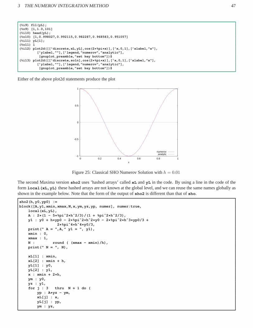
3 THE NUMEROV INTEGRATION METHOD 47
(%i9) fll(yL);(%o9) [1,1.0,101](%i10) head(yL);(%o10) [1,0.998027,0.992115,0.982287,0.968583,0.9510 57](%i11) yL[1];(%o11) 1(%i12) plot2d([[’discrete,xL,yL],cos(2 * %pi * x)],[’x,0,1],[’xlabel,"x"],
[’ylabel,""],[’legend,"numerov","analytic"],[gnuplot_preamble,"set key bottom"])$
(%i13) plot2d([[’discrete,soln],cos(2 * %pi * x)],[’x,0,1],[’xlabel,"x"],[’ylabel,""],[’legend,"numerov","analytic"],
[gnuplot_preamble,"set key bottom"])$
Either of the above plot2d statements produce the plot
-1
-0.5
0
0.5
1
0 0.2 0.4 0.6 0.8 1
x
numerovanalytic
Figure 25: Classical SHO Numerov Solution withh = 0.01
The second Maxima versionsho2 uses ’hashed arrays’ calledxL andyL in the code. By using a line in the code of theform local(xL,yL) these hashed arrays are not known at the global level, and we can reuse the same names globally asshown in the example below. Note that the form of the output ofsho2 is different than that ofsho .
sho2(h,y0,yp0) :=block([A,y1,xmin,xmax,N,x,ym,yz,yp, numer], numer:tru e,
local(xL,yL),A : 2 * (1 - 5 * %piˆ2 * hˆ2/3)/(1 + %piˆ2 * hˆ2/3),y1 : y0 + h * yp0 - 2 * %piˆ2 * hˆ2 * y0 - 2 * %piˆ2 * hˆ3 * yp0/3 +
2* %piˆ4 * hˆ4 * y0/3,print(" A = ",A," y1 = ", y1),xmin : 0,xmax : 1,N : round ( (xmax - xmin)/h),print(" N = ", N),
xL[1] : xmin,xL[2] : xmin + h,yL[1] : y0,yL[2] : y1,x : xmin + 2 * h,ym : y0,yz : y1,for j : 3 thru N + 1 do (
yp : A * yz - ym,xL[j] : x,yL[j] : yp,ym : yz,

3 THE NUMEROV INTEGRATION METHOD 48
yz : yp,x : x + h ),
[ listarray(xL), listarray(yL) ] )$
We use the same input parameters as before in this example. Toemphasize the fact that the code linelocal(xL,yL)
hides the values assigned to the hashed arrays, we first useremvalue to remove the definition of the listsxL andyL
produced in the example above.
(%i14) remvalue(xL, yL);(%o14) [xL,yL](%i15) xL[1];(%o15) xL[1](%i16) yL[1];(%o16) yL[1](%i17) soln : sho2(0.01, 1, 0)$
A = 1.9960535 y1 = 0.998027N = 100
(%i18) xL[1];(%o18) xL[1](%i19) xL : soln[1]$(%i20) fll(xL);(%o20) [0,1.0,101](%i21) head(xL);(%o21) [0,0.01,0.02,0.03,0.04,0.05](%i22) yL[1];(%o22) yL[1](%i23) yL : soln[2]$(%i24) fll(yL);(%o24) [1,1.0,101](%i25) plot2d([[’discrete,xL,yL],cos(2 * %pi * x)],[’x,0,1],[’xlabel,"x"],
[’ylabel,""],[’legend,"numerov","analytic"],[gnuplot_preamble,"set key bottom"])$
which produces exactly the same plot as produced usingsho .
3.1.2 Classical SHO Numerov Method Using R
The file cp3.R contains a functionsho(h,y0,yp0) with the same input syntax as the Maxima version. But the Rfunction returns a R list:list(xL, yL) in whichxL is a vector containing thex positions, andyL is a vector containingthe correspondingy values produced by the Numerov code.
## sho(h,y0,yp0)
## integrates simple harmonic oscillator with unit period## dˆ2y/dxˆ2 = - 4 piˆ2 y(x) over [x,0,1]## using the numerov method.## Input: h = step size, y0 = y(0), yp0 = y’(0)## Output: list( xL, yL)
sho = function(h,y0,yp0) {A = 2* (1 - 5 * piˆ2 * hˆ2/3)/(1 + piˆ2 * hˆ2/3)y1 = y0 + h * yp0 - 2 * piˆ2 * hˆ2 * y0 - 2 * piˆ2 * hˆ3 * yp0/3 +
2* piˆ4 * hˆ4 * y0/3xmin = 0xmax = 1N = (xmax - xmin)/hyL = vector(length = N + 1)xL = vector(length = N + 1)xL[1] = xminxL[2] = xmin + hyL[1] = y0yL[2] = y1
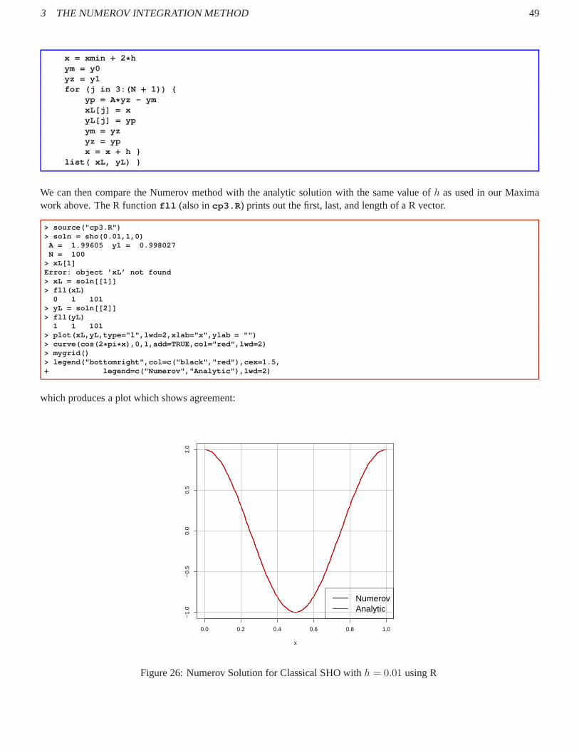
3 THE NUMEROV INTEGRATION METHOD 49
x = xmin + 2 * hym = y0yz = y1for (j in 3:(N + 1)) {
yp = A* yz - ymxL[j] = xyL[j] = ypym = yzyz = ypx = x + h }
list( xL, yL) }
We can then compare the Numerov method with the analytic solution with the same value ofh as used in our Maximawork above. The R functionfll (also incp3.R ) prints out the first, last, and length of a R vector.
> source("cp3.R")> soln = sho(0.01,1,0)
A = 1.99605 y1 = 0.998027N = 100
> xL[1]Error: object ’xL’ not found> xL = soln[[1]]> fll(xL)
0 1 101> yL = soln[[2]]> fll(yL)
1 1 101> plot(xL,yL,type="l",lwd=2,xlab="x",ylab = "")> curve(cos(2 * pi * x),0,1,add=TRUE,col="red",lwd=2)> mygrid()> legend("bottomright",col=c("black","red"),cex=1.5,+ legend=c("Numerov","Analytic"),lwd=2)
which produces a plot which shows agreement:
0.0 0.2 0.4 0.6 0.8 1.0
−1.
0−
0.5
0.0
0.5
1.0
x
NumerovAnalytic
Figure 26: Numerov Solution for Classical SHO withh = 0.01 using R

4 THE LENNARD JONES 6-12 POTENTIAL WELL: ENERGY LEVELS AND WAVE FUNCTIONS 50
4 The Lennard Jones 6-12 Potential Well: Energy Levels and Wave Functions
The Lennard Jones 6-12 potential (energy) can be defined by
V (r) = 4V0
[
(a
r
)12
−(a
r
)6]
, (4.1)
in which a is an adjustable length,V0 is an adjustable energy andr ≥ 0. We used the quasi-classical WKB method inExample 1 of this series to estimate the lowest molecular energy levels associated with this potential.
We define a dimensionless coordinatex = r/a, a dimensionless potential energyV = V/V0 and energyE = E/V0 anda dimensionless wave functionψ(x) =
√aψ(x), in terms of which we have a dimensionless potential (energy)
V (x) = 4
[
1
x12− 1
x6
]
(4.2)
and Schroedinger’s equation takes the form
d2 ψ(x)
d x2+ γ2
(
E − V (x))
ψ(x) = 0, (4.3)
in which the dimensionless parameter
γ =
[
2ma2 V0~2
]1/2
. (4.4)
The wave function normalization condition becomes∫
∞
0
ψ(x)2 d x = 1. (4.5)
In Example 1 we used the caseγ = 50, which we will also use here.
In the following, we omit the tildes and usey(x) to representψ(x).
4.1 The Numerov Method Using Maxima
The file LJ6-12.mac contains a group of Maxima functions designed to explore theenergy levels and wave functionsassociated with a quantum particle in the Lennard-Jones 6/12 potential introduced in the previous section. The dimen-sionless parameterγ takes on the same value as used for our quasi-classical limitapproach in Example 1 of this series,andgam2 in our code representsγ2.
The dimensionless potential (energy)V (x) does not depend on the value ofγ and we can make a simple plot and exploreits shape. After defining a function which is based on the formof V (x), we define the value ofx, calledxm, whereV (x)takes on its minimum value, and show thatV (xm) = −1, V (1) = 0, andV (x) approaches large positive values asx approaches0, and small negative values forx very large. Recall that nowx represents a non-negative dimensionlessnumber.
(%i1) V(z) := ( 4 * (zˆ(-12) - zˆ(-6)) )$(%i2) xm : float(2ˆ(1/6));(%o2) 1.122462048309373(%i3) V(xm);(%o3) -1.0(%i4) V(1);(%o4) 0(%i5) V(0.5);(%o5) 16128.0(%i6) V(3);(%o6) -2912/531441(%i7) float(%);

4 THE LENNARD JONES 6-12 POTENTIAL WELL: ENERGY LEVELS AND WAVE FUNCTIONS 51
(%o7) -0.0054794417442388(%i8) V(0.1);(%o8) 3.9999959999999946E+12(%i9) V(10.0);(%o9) -3.9999959999999997E-6%i10) limit(V(x),x,inf);(%o10) 0(%i11) limit( V(x),x,0,plus );(%o11) inf(%i12) plot2d([ [discrete,[ [0.8,0],[2,0]]], V(x)],
[x,0.8,2],[y,-1.5,2], [xlabel,"x"],[ylabel,"V(x)"],[style, [lines,3]],[legend,false],[gnuplot_preamble, "set grid"])$
plot2d: some values were clipped.
which produces the dimensionless potential (energy) plot:
-1.5
-1
-0.5
0
0.5
1
1.5
2
0.8 1 1.2 1.4 1.6 1.8 2
V(x
)
x
Figure 27: Dimensionless Lennard Jones Potential (Energy)
The bound state energy eigenvalues lie in the range−1 < E < 0 and the classical turning points are defined by theequationE = V (x). Settingy = x6, one obtains a quadratic equation iny which is easily solved forytp. One can then
obtain the classical turning points as a function ofE from xtp = y1/6tp . Bearing in mind thatE < 0, we can write the
turning points in Maxima code as
(%i13) xin(E) := xm * (sqrt(E+1)/E-1/E)ˆ(1/6)$(%i14) xout(E) := xm * (sqrt(E+1)+1)ˆ(1/6)/(-E)ˆ(1/6)$
and then one can add a hypothetical energy level line to our potential energy plot:
(%i15) plot2d([ [discrete,[ [0.8,0],[2,0]]], V(x),[discrete, [ [xin(-0.5),-0.5],[xout(-0.5),-0.5] ]] ],[x,0.8,2],[y,-1.5,2], [xlabel,"x"],[ylabel,"V(x)"],
[style, [lines,3]],[legend,false],[gnuplot_preamble, "set grid"])$plot2d: some values were clipped.
which produces the plot
-1.5
-1
-0.5
0
0.5
1
1.5
2
0.8 1 1.2 1.4 1.6 1.8 2
V(x
)
x
Figure 28: Adding a Hypothetical Energy Level

4 THE LENNARD JONES 6-12 POTENTIAL WELL: ENERGY LEVELS AND WAVE FUNCTIONS 52
Loading in the fileLJ6-12.mac defines a set of global parameters and functions defined at thetop of the file:
/ * initial global parameters: * /
( h : 0.01,h2 : hˆ2/12, / * Numerov constants * /h52 : 5 * h2,gam2 : 2500, / * square of gam = 50 * /x1decay : 0.3, / * start yL integration at (x1 - x1decay) * /x2decay : 1, / * start yR integration at (x2 + x2decay) * /y2left : 1e-19, / * y(x_left + h) value chosen from E = -0.9 case * /y2right : 1e-16, / * y(x_right - h) value chosen from E = -0.9 case * /print(" gam2 = ", gam2),print(" h = ", h, ", x1decay = ", x1decay, ", x2decay = ", x2deca y),print(" y2left = ",y2left, " y2right = ", y2right ),xm : float(2ˆ(1/6)), / * this is where V(x) = -1 = minimum value * // * for given energy -1 < E < 0 , these are the turning points * /xin(E) := xm * (sqrt(E+1)/E-1/E)ˆ(1/6),xout(E) := xm * (sqrt(E+1)+1)ˆ(1/6)/(-E)ˆ(1/6),/ * dimensionless potential V(x) for Lennard-Jones 6/12 poten tial * /V(z) := ( 4 * (zˆ(-12) - zˆ(-6)) ) )$
The grid sizeh and two Numerov method constantsh2 and h52 which depend onh are then globally available. Wecall the left classical turning pointx1 and we start the rightward Numerov integration at positionx1 - x1decay withy = 0. Likewise we call the right classical turning pointx2 and start the leftward Numerov integration at positionx2 + x2decay with y = 0.
(%i1) load(cp3);(%o1) "c:/k3/cp3.mac"(%i2) load("LJ6-12.mac");
gam2 = 2500h = 0.01 , x1decay = 0.3 , x2decay = 1y2left = 1.0E-19 y2right = 1.0E-16
(%o2) "c:/k3/LJ6-12.mac"
Let us ignore, at first, some slight refinements we have in the code, and give a simplified version.
We first define a grid pointx2c which is close to the right classical turning pointx2 .
We next generate a list calledyL which contains the values ofy(x) from the grid pointx_left : x1 - x1decay , withy(xleft) = 0, andy(xleft + h) = y2left , and further points generated using the Numerov method, continuing to thegrid pointx2c + h .
Next we generate a list calledyR which contains the values ofy(x) from x2 + x2decay , with y(xright) = 0, andy(xright−h) = y2right , and further points generated using the Numerov method, continuing to the grid pointx2c - h .
We then multiply all values ofyL by a common factor which ensures thatyL andyR agree on the value ofy(x = x2c) .
The x grid valuesxL andxR, and the correspondingy(x) grid values contained in the listsyL andyR are available asglobal quantities.
Here is code forwf(E) from LJ6-12.mac that generates the un-normalized wave functions in the formof the globallists xL , yL , xR, yR. In the functionwf(E) we use the hashed arraysxl , yl , xr , andyr . Their names are included in alocal statement of the formlocal(g,xl,yl,xr,yr) , so that the hashed arrays are not available at the global level.At the end ofwf(E) we have statements such asxL : listarray(xl) andyL : listarray(yl) , which make thecontents of the hashed arrays available as ordinary lists globally.

4 THE LENNARD JONES 6-12 POTENTIAL WELL: ENERGY LEVELS AND WAVE FUNCTIONS 53
/ * wf(E) creates ** un-normalized ** wave functionsfor the Lennard-Jones 6/12 potential case.limits of numerical integration, x_left and x_right aredetermined by energy E and xdecay values.The wave functions are stored in global xL, yL, xR, yR.Program also defines ** global ** x2c, nleft, nright, x_left, x_right.See example run at end.
nleft = the number of steps from x_left to x2c = grid point near est tox1 = xin(E) = classical turning point < xm = 1.122462x2 = xout(E) = classical turning point > xm.the global xL grid extends from x_left to x2c + h andthe global xR grid extends from x2c - h to x_right,so we can compute y’(x2c) using a 3 pt. symmetric formula.
* /
wf(E) := block( [x1,x2,x, fac,numer],numer:true,if (E > 0) or (E < -1) then (
print(" need -1 < E < 0 "),return(false)),
local(g,xl,yl,xr,yr),g(z) := gam2 * ( E - V(z) ), / * coeff. func. in ode: y’’(x) + g(x) y(x) = 0 * /x1 : xin(E), / * classical turning point for x < xm * /x2 : xout(E), / * classical turning point for x> xm * /if wfdebug then print(" x1 = ", x1, " x2 = ", x2),x_left : x1 - x1decay,nleft : round ( (x2 - x_left)/h ), / * number of steps from x_left to x2c = match point * /x2c : x_left + h * nleft,if wfdebug then print(" x_left = ",x_left," nleft = ",nleft, " x2c = ", x2c),if wfdebug then print(" y2left = ", y2left, " y2right = ", y2ri ght),nright : round ( (x2 + x2decay - x2c)/h ), / * number of steps from x2c to x_right * /x_right : x2c + h * nright,if wfdebug then print(" nright = ",nright," x_right = ",x_ri ght),/ * find yL for x_left <= x <= x2c + h using Numerov algorithm * /xl[1] : x_left,xl[2] : x_left + h,yl[1] : 0,yl[2] : y2left,for j:2 thru nleft + 1 do (
x : x_left + j * h,xl[j+1] : x,yl[j+1] : ( 2 * (1 - h52 * g(x-h)) * yl[j] - (1 + h2 * g(x-2 * h)) * yl[j-1] )/ (1 + h2 * g(x)) ),
/ * find yR for x2c - h <= x <= x_right using Numerov method * /xr[nright + 2 ] : x_right,xr[nright + 1] : x_right - h,yr[nright + 2] : 0,yr[nright + 1] : y2right,for j:nright+1 step -1 thru 2 do (
x : x2c + h * (j -3),xr[j-1] : x,yr[j-1] : (2 * (1-h52 * g(x+h)) * yr[j] - (1 + h2 * g(x+2 * h)) * yr[j+1] )/(1 + h2 * g(x)) ),
fac : yr[2]/yl[nleft + 1], / * yR(x2c) / yL(x2c) * /for j thru nleft+2 do yl[ j ] : fac * yl[ j ],xL : listarray(xl),yL : listarray(yl),xR : listarray(xr),yR : listarray(yr),done)$
4 THE LENNARD JONES 6-12 POTENTIAL WELL: ENERGY LEVELS AND WAVE FUNCTIONS 54
An example of the use ofwf(E) for a randomly chosen energy is
(%i3) wf(-0.5);(%o3) done(%i4) fll(xL);(%o4) [0.726743,1.3867425,67](%i5) fll(xR);(%o5) [1.3667425,2.3767425,102](%i6) head(yL);(%o6) [0,1.75654725E-29,-3.97814273E-28,1.06730999E- 26,-3.66490209E-25,
1.85515641E-23](%i7) tail(yL);(%o7) [1.46282504E-4,4.50817194E-4,7.49059762E-4,0.0 0104033,0.00132673,0.00161295](%i8) dy_diff();(%o8) 33.121756(%i9) num_nodes();(%o9) 3
The functiondy_diff() used above is designed to return the difference of the approximate numerical first derivatives atthe matching pointx2c implied byyL andyR, divided by the value ofy(x2c) . Here is our code fordy_diff() .
/ * dy_diff() uses global yL, yR,nleft, hcomputes numerical y’(x2c) usingsymmetric three point method forboth yL and yR, and returns the differencedivided by y(x2c)
* /
dy_diff() :=block([ypL, ypR, numer],numer:true,
ypL : ( last(yL) - yL[nleft] ) / (2 * h),ypR : (yR[3] - first(yR)) / (2 * h),(ypL - ypR)/ abs (yR[2]) )$
The functionnum_nodes() has the definition:
/ * count the number of nodes in yLignore region where elements of yL aretiny in magnitude.uses position(...) * /
num_nodes() :=block([x11, j0, yLm2, n, numer], numer:true,
x11 : x_left + x1decay,j0 : position(x11, xL),yLm2 : rest(yL,-2), / * ignore y(x2c) and y(x2c+h) values in count * /n : 0,for j : j0 thru (length(yLm2) - 1) do
if yLm2[j] * yLm2[j + 1] < 0 then n : n + 1,n)$
and usesposition(...) :
/ * position(xv, aL) is designed to be used with xL to locateposition of first element which is equal to or greater than x1 ,since in this package xL has just increasing positive number s in it
* /
position(xv, aL) := ( first (sublist_indices(aL,lambda([ x], x >= xv))))$

4 THE LENNARD JONES 6-12 POTENTIAL WELL: ENERGY LEVELS AND WAVE FUNCTIONS 55
We search for energy eigenvalues by seeking energiesE such that the value returned bydy_diff() is zero to withinnumerical errors. A functionF(E) allows us to scan energy ranges for energy eigenvalues.
/ * energy eigenvalue if global function F(E) = 0 .F(E) calls wf(E) then returns dy_diff(), butreturns false if E > 0.
* /
F(E) :=block( [ numer],numer:true,
if E > 0 then (print(" in F(E), E = ",E," should be negative "),return(false)),
wf(E),dy_diff())$
Here is an example of usingF(E) .
(%i10) EL : makelist(e,e,-0.91,-0.85,0.01);(%o10) [-0.91,-0.9,-0.89,-0.88,-0.87,-0.86,-0.85](%i11) FL : map(F,EL);(%o11) [7.199669,2.035782,-5.228712,-24.50145,-58.60 732,232.5781,61.42046](%i12) F(-0.91);(%o12) 7.1996689(%i13) F(-0.88);(%o13) -24.501452(%i14) e : find_root(F, -0.91,-0.88);(%o14) -0.896404
A function wf_plot(E) generates a non-normalized numerical solution usingwf(E) , makes a plot and prints out theenergy and maximum y value, the number of nodes, and the valueof dy_diff() corresponding to the chosen energyE.
(%i15) wf_plot(e);E = -0.896404 , ymax = 27.422334number of nodes = 0 , dy_diff = 7.94875172E-14
which produces the plot
0
5
10
15
20
25
0.6 0.8 1 1.2 1.4 1.6 1.8 2 2.2 2.4
y
x
Figure 29: Zero Nodes Un-normalized Eigenfunction

4 THE LENNARD JONES 6-12 POTENTIAL WELL: ENERGY LEVELS AND WAVE FUNCTIONS 56
The code forwf_plot(E) is
/ *wf_plot (E) calls wf(E) and plot2dcreates ** un-normalized ** wave functionsstored in global xL, yL, xR, yR.prints out number of nodes in yLprints out dy_diff .
* /
wf_plot(E) :=block([xxL, yyL, ymn,ymx, numer], numer:true,
wf(E),xxL : rest(xL, -1),yyL : rest(yL, -1),ymn : float( floor ( lmin(yyL))),ymx : float(1 + floor ( lmax(yyL))),print( " E = ", E, ", ymax = ", lmax(yyL) ),print(" number of nodes = ",num_nodes(), ", dy_diff = ",dy_d iff() ),plot2d([ [discrete, xxL, yyL], [discrete, rest(xR,1), res t(yR,1)] ],
[y,ymn,ymx], [ylabel,"y"], [xlabel,"x"], [style, [lines ,3]],[legend, false], [gnuplot_preamble,"set grid"]))$
We then create (fromyL andyR) a global normalized wave function listyn corresponding to a global grid listxn createdfrom xL and xR using the functionnormalize() . This function also computes and prints the value of the quantummechanical particle position uncertainty∆x implied by the wave function.
(%i16) normalize();AA = 85.006868x_mean = 1.1406875delx = 0.0455039
(%o16) done(%i17) fll(xn);(%o17) [0.781455,2.2014549,143](%i18) fll(yn);(%o18) [-3.14183197E-20,0,143](%i19) lmax(yL);(%o19) 27.422334(%i20) lmax(yn);(%o20) 2.9742495
The functionnormalize uses our utility functionssimp (Simpson’s one third integration rule) andmerge .
/ * normalize() uses the current global xL,yL, xR, yR andthe utility functions merge and simp to define globalxn and yn, with the latter being normalized.
* /
normalize() :=block ( [AA,x_mean,x2_mean,delx,delx2, numer ], numer:tr ue,
xn : merge( rest(xL,-1), rest(xR, 2) ),yn : merge( rest(yL,-1), rest(yR, 2) ),/ * we need xn to have odd # of elements to use simp * /if evenp ( length (xn) ) then (
xn : rest (xn),yn : rest (yn)),
AA : simp(xn,ynˆ2),print( " AA = ",AA),yn : yn/sqrt(AA),x_mean : simp(xn, xn * ynˆ2),print(" x_mean = ", x_mean),x2_mean : simp(xn, xnˆ2 * ynˆ2),delx2 : x2_mean - x_meanˆ2, / * this should be positive! * /

4 THE LENNARD JONES 6-12 POTENTIAL WELL: ENERGY LEVELS AND WAVE FUNCTIONS 57
delx : sqrt(delx2),print(" delx = ", delx),done)$
Oncenormalize() has been used to createxn and yn from the current un-normalized wave function, we can useyn_plot_current() to see the current normalized wave function.
(%i21) yn_plot_current()$ymax = 2.9742495
which produces the plot
-1
-0.5
0
0.5
1
1.5
2
2.5
3
0.6 0.8 1 1.2 1.4 1.6 1.8 2 2.2 2.4
y
x
Figure 30: Zero Node Normalized Eigenfunction
A function yn_plot(E, xmin, xmax) goes from a given energyE to a call towf(E) andnormalize() and thenmakes a plot of the resulting normalized wave function in onestep, with control over the region of thex axis for the plot.Thus
(%i22) yn_plot(e,0.8, 1.6)$E = -0.896404number of nodes = 0 , dy_diff = 7.94875172E-14AA = 85.006868x_mean = 1.1406875delx = 0.0455039normalized ymax = 2.9742495
produces the plot
-1
-0.5
0
0.5
1
1.5
2
2.5
3
0.8 0.9 1 1.1 1.2 1.3 1.4 1.5 1.6
y
x
Figure 31: Using ynplot(E,xmin,xmax) forE = −0.896404
Here is an example of usingyn_plot for an energy which is not an energy eigenvalue. The value ofdy_diff() reportedis based on the non-normalized wave function produced bywf(E) .
(%i23) yn_plot(-0.95,0.8, 1.6)$E = -0.95number of nodes = 0 , dy_diff = 16.398098AA = 139.33333x_mean = 1.1545679delx = 0.0420213normalized ymax = 3.2673444

4 THE LENNARD JONES 6-12 POTENTIAL WELL: ENERGY LEVELS AND WAVE FUNCTIONS 58
which produces the plot
0
0.5
1
1.5
2
2.5
3
3.5
4
0.8 0.9 1 1.1 1.2 1.3 1.4 1.5 1.6
y
x
Figure 32: Using ynplot(E,xmin,xmax) forE = −0.95
We see a large discontinuity in the slope of the normalized wave function, reflected also in the large value ofdy_diff()
reported in the non-normalized wave function.
Here is the code foryn_plot :
yn_plot(E,xmn,xmx) :=block([ymn, ymx, numer],numer:true,
wf(E),print(" E = ",E ),print(" number of nodes = ",num_nodes(),", dy_diff = ",dy_d iff() ),normalize(),print(" normalized ymax = ", lmax(yn) ),ymn : floor( lmin(yn) ),ymx : 1 + floor( lmax (yn) ),plot2d( [discrete, xn, yn], [’x,xmn, xmx],
[’y,ymn,ymx], [ylabel,"y"], [xlabel,"x"],[style, [lines, 3] ], [legend, false], [gnuplot_preamble, "set grid"]))$
A plot of the values ofF(E) over a wider energy range will show other candidate energiesfor excited states havingenergies greater than the ground state (zero node state withenergyE0 = −0.896404 found above). However, use of thefunction bracket(Estart,dE,Eacc) is an easier way to find candidate energy eigenvalues.bracket looks for thefirst sign change inF(E) , and (in a normal exit) returns a pair of energies for whichF(E) has the opposite sign. Applyingthis approach to the ground state energy found above,
(%i23) [ea,eb]:bracket(F,-0.96,0.02,0.01);(%o23) [-0.9,-0.895](%i24) e: find_root(F,ea,eb);(%o24) -0.896404(%i25) yn_plot(e,0.8,1.6)$
E = -0.896404number of nodes = 0 , dy_diff = -1.33606678E-13AA = 85.006868x_mean = 1.1406875delx = 0.0455039normalized ymax = 2.9742495
which results in the same plot as we displayed above for the normalized ground state.
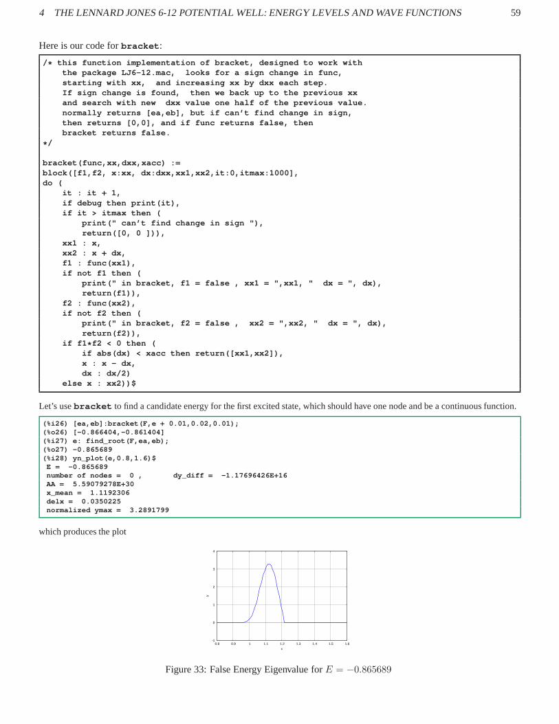
4 THE LENNARD JONES 6-12 POTENTIAL WELL: ENERGY LEVELS AND WAVE FUNCTIONS 59
Here is our code forbracket :
/ * this function implementation of bracket, designed to work w iththe package LJ6-12.mac, looks for a sign change in func,starting with xx, and increasing xx by dxx each step.If sign change is found, then we back up to the previous xxand search with new dxx value one half of the previous value.normally returns [ea,eb], but if can’t find change in sign,then returns [0,0], and if func returns false, thenbracket returns false.
* /
bracket(func,xx,dxx,xacc) :=block([f1,f2, x:xx, dx:dxx,xx1,xx2,it:0,itmax:1000],do (
it : it + 1,if debug then print(it),if it > itmax then (
print(" can’t find change in sign "),return([0, 0 ])),
xx1 : x,xx2 : x + dx,f1 : func(xx1),if not f1 then (
print(" in bracket, f1 = false , xx1 = ",xx1, " dx = ", dx),return(f1)),
f2 : func(xx2),if not f2 then (
print(" in bracket, f2 = false , xx2 = ",xx2, " dx = ", dx),return(f2)),
if f1 * f2 < 0 then (if abs(dx) < xacc then return([xx1,xx2]),x : x - dx,dx : dx/2)
else x : xx2))$
Let’s usebracket to find a candidate energy for the first excited state, which should have one node and be a continuous function.
(%i26) [ea,eb]:bracket(F,e + 0.01,0.02,0.01);(%o26) [-0.866404,-0.861404](%i27) e: find_root(F,ea,eb);(%o27) -0.865689(%i28) yn_plot(e,0.8,1.6)$
E = -0.865689number of nodes = 0 , dy_diff = -1.17696426E+16AA = 5.59079278E+30x_mean = 1.1192306delx = 0.0350225normalized ymax = 3.2891799
which produces the plot
-1
0
1
2
3
4
0.8 0.9 1 1.1 1.2 1.3 1.4 1.5 1.6
y
x
Figure 33: False Energy Eigenvalue forE = −0.865689

4 THE LENNARD JONES 6-12 POTENTIAL WELL: ENERGY LEVELS AND WAVE FUNCTIONS 60
The plot shows a discontinuous zero node wave function and the reported value ofdy_diff() is not a tiny number, asdy_diff() should be for a valid energy eigenvalue case. We also note that we had already found a valid zero nodeenergy eigenvalue.
Continuing with a search for energy eigenvalues usingbracket :
(%i29) [ea,eb]:bracket(F,e + 0.01,0.02,0.01);(%o29) [-0.710689,-0.705689](%i30) e : find_root(F,ea,eb);(%o30) -0.71066(%i31) yn_plot(e,0.8,1.6)$
E = -0.71066number of nodes = 1 , dy_diff = 8.68128554E-15AA = 0.0295798x_mean = 1.1806289delx = 0.0807403normalized ymax = 2.6000666
which produces a valid one node wave function
-3
-2
-1
0
1
2
3
0.8 0.9 1 1.1 1.2 1.3 1.4 1.5 1.6
y
x
Figure 34: One Node Wave Function forE = −0.71066
This one node wave function is continuous and the reported value of dy_diff() is a tiny number.
We will again find a spurious one node solution at a slightly higher energy. However, we must reduce the size of thedE argument tobracket .
(%i32) [ea,eb]:bracket(F,e + 0.01,0.02,0.01);(%o32) [-0.71066,-0.70566](%i33) [ea,eb]:bracket(F,e + 0.02,0.02,0.01);(%o33) [-0.71066,-0.70566](%i34) [ea,eb]:bracket(F,e + 0.02,0.01,0.005);(%o34) [-0.68566,-0.68316](%i35) e : find_root(F,ea,eb);(%o35) -0.684654(%i36) yn_plot(e,0.8,1.6)$
E = -0.684654number of nodes = 1 , dy_diff = 4.23941273E+16AA = 3.63949121E+28x_mean = 1.1531148delx = 0.0706492normalized ymax = 2.5594982

4 THE LENNARD JONES 6-12 POTENTIAL WELL: ENERGY LEVELS AND WAVE FUNCTIONS 61
which shows a spurious one node wave function (note the very large value ofdy_diff ):
-3
-2
-1
0
1
2
3
0.8 0.9 1 1.1 1.2 1.3 1.4 1.5 1.6
y
x
Figure 35: False Energy Eigenvalue forE = −0.684654
Now that we see the pattern of valid energy eigenvalues, we can write a functionlevels(Emin,Emax,dE, Eacc) , which usesbracket with the added filter that no sign change ofF(E) is taken seriously unless the associated wave function has one morenode than the last energy eigenvalue found.
/ * levels(Emin,Emax,dE, Eacc ) returns a list [Ea, Eb,...] of e nergy levels withincreasingly larger number of nodes in energy range (Emin, E max).
uses F(E) to find roots, and calls wf, num_nodes() and dy_dif f() for each root found,Uses bracket and find_root.The arguments (dE, Eacc) are used to call bracket, and do not d escribe
the accuracy of the energy levels found.Once a good energy e.v. is found we look for the region of
energies with one more node and search there.Code inclues an interactive continue or stop prompt.
* /
levels(Emin,Emax,dE, Eacc ) :=block([ e,enext, eroot, eL, ea, eb, nn, nlast : -1, r, numer], numer:true,
e : Emin,eL : [ ], / * list eL will hold energy eigenvalues found * /do ( if e > Emax then return(), / * exit do loop * /
print("---------------- levels -------------------"),print(" nlast = ", nlast),print(" Estart = ", e," dE = ", dE ),[ea, eb] : bracket(F,e, dE, Eacc),print(" ea = ",ea," eb = ",eb),if float(ea) = 0.0 then (
print(" can’t find bracket interval "),print(" e = ",e),return() ),
eroot : find_root(F, ea, eb),print(" eroot = ", eroot),wf(eroot),nn : num_nodes(),print(" number of nodes = ", nn),print(" dy_diff at x2c = ", dy_diff() ),eL : cons(eroot, eL),nlast : nn,r : read (" input c; or s; "),if string(r) = "s" then return(), / * exit do loop * /

4 THE LENNARD JONES 6-12 POTENTIAL WELL: ENERGY LEVELS AND WAVE FUNCTIONS 62
/ * search for an energy greater than eb which producesa wave function with nn + 1 nodes * /
enext : eb + dE,do (
wf(enext),if num_nodes() > nlast then (
e : enext,return() )
else enext : enext + dE)),reverse(eL) )$
Here is an example of use:
(%i37) levels(-0.95, -0.6, 0.02,0.01);---------------- levels -------------------
nlast = -1Estart = -0.95 dE = 0.02ea = -0.9 eb = -0.895eroot = -0.896404number of nodes = 0dy_diff at x2c = -5.41191607E-14input c; or s;
c;---------------- levels -------------------
nlast = 0Estart = -0.835 dE = 0.02ea = -0.715 eb = -0.71eroot = -0.71066number of nodes = 1dy_diff at x2c = 1.73625711E-14input c; or s;
c;---------------- levels -------------------
nlast = 1Estart = -0.67 dE = 0.02ea = -0.555 eb = -0.55eroot = -0.551436number of nodes = 2dy_diff at x2c = -7.17260262E-15input c; or s;
c;(%o37) [-0.896404,-0.71066,-0.551436](%i38) [E0,E1,E2] : %;(%o38) [-0.896404,-0.71066,-0.551436]
We then can useyn_plot for the ground state energy to create the normalized wave function and make a plot, and usingxyn0 = makelist(...) to save these wave function definitions under a unique name.
(%i39) yn_plot(E0,0.8,1.6)$E = -0.896404number of nodes = 0 , dy_diff = -5.41191607E-14AA = 85.006868x_mean = 1.1406875delx = 0.0455039normalized ymax = 2.9742495
(%i40) xyn0 : makelist([xn[j],yn[j]],j,1,length(xn))$(%i41) fll(xyn0);(%o41) [[0.781455,-3.14183197E-20],[2.2014549,0],143 ]
We can then continue with the first and second excited states.
(%i42) yn_plot(E1,0.8,1.6)$E = -0.71066number of nodes = 1 , dy_diff = 1.98222687E-13AA = 0.0295798x_mean = 1.1806289delx = 0.0807403normalized ymax = 2.6000666
(%i43) xyn1 : makelist([xn[j],yn[j]],j,1,length(xn))$

4 THE LENNARD JONES 6-12 POTENTIAL WELL: ENERGY LEVELS AND WAVE FUNCTIONS 63
(%i44) fll(xyn1);(%o44) [[0.754761,2.83787145E-25],[2.2747607,0],153](%i45) yn_plot(E2,0.8,1.6)$
E = -0.551436number of nodes = 2 , dy_diff = 2.03223741E-13AA = 1.24980723E-5x_mean = 1.2265982delx = 0.108671normalized ymax = 2.4452266
(%i46) xyn2 : makelist([xn[j],yn[j]],j,1,length(xn))$(%i47) fll(xyn2);(%o47) [[0.730536,0],[2.3505359,0],163]
We can finally make a plot of the three normalized wave functions corresponding to the lowest three energy levels in the Lennard-Jones potential.
(%i48) plot2d([[discrete,xyn0],[discrete,xyn1],[disc rete,xyn2]],[x,0.8,1.6],[xlabel,"x"],[ylabel,"y"],[style,[lines ,2]],
[legend,"E0","E1","E2"])$
which produces the plot
-3
-2
-1
0
1
2
3
0.8 0.9 1 1.1 1.2 1.3 1.4 1.5 1.6
y
x
E0E1E2
Figure 36: Lennard-Jones: Wave Functions for Lowest Three Energy Levels
As we did with the finite potential well case, we can save the energies and wave functions usingsave(filename,a1,a2,...)for use in a later, different Maxima session.
(%i49) save("c:/k3/LJ1.dat",E0,xyn0,E1,xyn1,E2,xyn2) ;(%o49) "c:/k3/LJ1.dat"
The top of this data file, viewed with a text editor, is writtenin Lisp, and looks like:
;;; - * - Mode: LISP; package:maxima; syntax:common-lisp; - * -(in-package :maxima)(DSKSETQ |$e0| -0.89640379037496043)(ADD2LNC ’|$e0| $VALUES)(DSKSETQ $XYN0
’((MLIST SIMP)((MLIST SIMP) 0.78145488500192117 -3.1418319670117798E -20)((MLIST SIMP) 0.79145488500192118 7.7629000010676559E- 18)((MLIST SIMP) 0.80145488500192119 8.9446105712810272E- 16)((MLIST SIMP) 0.8114548850019212 3.8907747472815292E-1 4)
etc., etc., ...

4 THE LENNARD JONES 6-12 POTENTIAL WELL: ENERGY LEVELS AND WAVE FUNCTIONS 64
If we start a new session of Maxima, we can useload to load in these saved definitions, and continue to use them asusual.
(%i1) load(cp3);(%o1) "c:/k3/cp3.mac"(%i2) load("LJ6-12.mac");
gam2 = 2500h = 0.01 , x1decay = 0.3 , x2decay = 1y2left = 1.0E-19 y2right = 1.0E-16
(%o2) "c:/k3/LJ6-12.mac"(%i3) load("LJ1.dat");(%o3) "c:/k3/LJ1.dat"(%i4) values;(%o4) [mydate,_binfo%,h,h2,h52,gam2,x1decay,x2decay, y2left,y2right,xm,E0,xyn0,
E1,xyn1,E2,xyn2](%i5) E0;(%o5) -0.896404(%i6) fll(xyn0);(%o6) [[0.781455,-3.14183197E-20],[2.2014549,0],143](%i7) plot2d([[discrete,xyn0],[discrete,xyn1],[discr ete,xyn2]],
[x,0.8,1.6],[xlabel,"x"],[ylabel,"y"],[style,[lines ,2]],[legend,"E0","E1","E2"])$
and we get the same plot as we did in the previous session.
A proper exploration of the likely accuracy of the energy levels found in this approach would involve experimenting withthe valuesof x1decay , x2decay , and the grid sizeh. One can modify the code so that the use of a five point symmetric formula for the firstderivative is used, instead of the present three point symmetric formula.
Increased integration accuracy can also be sought by writing a Numerov integration routine which uses big float arithmetic in theMaxima language to use 20 digit arithmetic, for example, rather than the default 16 digit arithmetic.
4.2 The Numerov Method Using R
The file LJ6-12.R contains a group of R functions designed to explore the energy levels and wave functions associated with aquantum particle in the Lennard-Jones 6/12 potential, using R. The dimensionless parameterγ = 50 takes on the same value as usedfor our quasi-classical limit approach in Example 1 of this series, andgam2 in our code representsγ2.
The dimensionless potential (energy)V (x) does not depend on the value ofγ and we can make a simple plot and explore its shape.After defining a function which is based on the form ofV (x), we define the value ofx, calledxm, whereV (x) takes on its minimumvalue, and show thatV (xm) = −1, V (1) = 0, andV (x) approaches large positive values asx approaches0, and small negativevalues forx very large. Recall that nowx represents a non-negative dimensionless number.
> V = function (x) 4 * (xˆ(-12) - xˆ(-6))> xm = 2ˆ(1/6); xm[1] 1.12246> V(xm)[1] -1> V(1)[1] 0> V(0.5)[1] 16128> V(3)[1] -0.00547944> V(0.1)[1] 4e+12> curve(V,0.8,2,lwd=3,col="red",ylim = c(-1.5,2),xlab= "x",ylab="y(x)")> lines(c(0.8,2),c(0,0),lwd=3,col="blue")> mygrid()

4 THE LENNARD JONES 6-12 POTENTIAL WELL: ENERGY LEVELS AND WAVE FUNCTIONS 65
which produces the dimensionless potential (energy) plot:
0.8 1.0 1.2 1.4 1.6 1.8 2.0
−1.
5−
1.0
−0.
50.
00.
51.
01.
52.
0
x
y(x)
Figure 37: Dimensionless Lennard Jones Potential (Energy)
The bound state energy eigenvalues lie in the range−1 < E < 0 and the classical turning points are defined by the equationE = V (x). Settingy = x6, one obtains a quadratic equation iny which is easily solved forytp. One can then obtain the classical
turning points as a function ofE from xtp = y1/6tp . Bearing in mind thatE < 0, we can write the turning points in R code as
> xin = function (E) xm * (sqrt(E+1)/E-1/E)ˆ(1/6)> xout = function (E) xm * (sqrt(E+1)+1)ˆ(1/6)/(-E)ˆ(1/6)
and then one can add a hypothetical energy level line to our potential energy plot:
> lines(c(xin(-0.5),xout(-0.5)), c(-0.5,-0.5), lwd = 3, c ol = "green")
which produces the plot
0.8 1.0 1.2 1.4 1.6 1.8 2.0
−1.
5−
1.0
−0.
50.
00.
51.
01.
52.
0
x
y(x)
Figure 38: Adding a Hypothetical Energy Level
4 THE LENNARD JONES 6-12 POTENTIAL WELL: ENERGY LEVELS AND WAVE FUNCTIONS 66
Loading in the fileLJ6-12.mac defines a set of global parameters and functions defined at thetop of the file:
## initial global parameters :
h = 0.01h2 = hˆ2/12 ## Numerov constantsh52 = 5 * h2gam2 = 2500 ## square of gam = 50x1decay = 0.3 ## start yL integration at (x1 - x1decay)x2decay = 1 ## start yR integration at (x2 + x2decay)y2left = 1e-19 ## y(x_left + h) value chosen from E = -0.9 casey2right = 1e-16 ## y(x_right - h) value chosen from E = -0.9 cas ecat (" gam2 = ", gam2, "\n")cat (" h = ", h, ", x1decay = ", x1decay, ", x2decay = ", x2decay, "\n")cat (" y2left = ",y2left, " y2right = ", y2right, "\n" )xm = 2ˆ(1/6) ## this is where V(x) = -1 = minimum value## for given energy -1 < E < 0 , these are the turning pointsxin = function (E) xm * (sqrt(E+1)/E-1/E)ˆ(1/6)xout = function (E) xm * (sqrt(E+1)+1)ˆ(1/6)/(-E)ˆ(1/6)## dimensionless potential V(x) for Lennard-Jones 6/12 pot entialV = function (x) 4 * (xˆ(-12) - xˆ(-6))wfdebug = FALSE
The grid sizeh and two Numerov method constantsh2 andh52 which depend onh are then globally available. We call the leftclassical turning pointx1 and we start the rightward Numerov integration at positionx1 - x1decay with y = 0. Likewise wecall the right classical turning pointx2 and start the leftward Numerov integration at positionx2 + x2decay with y = 0.
> source("cp3.R")> source("LJ6-12.R")
gam2 = 2500h = 0.01 , x1decay = 0.3 , x2decay = 1y2left = 1e-19 y2right = 1e-16
Let us ignore, at first, some slight refinements we have in the code, and give a simplified version.
We first define a grid pointx2c which is close to the right classical turning pointx2 .
We next generate a vector calledyl which contains the values ofy(x) from the grid pointx_left : x1 - x1decay , withy(xleft) = 0, andy(xleft + h) = y2left , and further points generated using the Numerov method, continuing to the grid pointx2c + h .
Next we generate a vector calledyr which contains the values ofy(x) from x2 + x2decay , with y(xright) = 0, andy(xright −h) = y2right , and further points generated using the Numerov method, continuing to the grid pointx2c - h .
We then multiply all values ofyl by a common factor which ensures thatyl andyr agree on the value ofy(x = x2c) .
Thex grid valuesxl andxr , and the correspondingy(x) grid values contained in the vectorsyl andyr are finally made availableas the global quantitiesxL , xR, yL , andyR respectively.
Here is code forwf(E) from LJ6-12.R that generates the un-normalized wave functions in the formof the global vectorsxL , yL ,xR, yR.
## wf(E) creates ** un-normalized ** wave functions## for the Lennard-Jones 6/12 potential case.## limits of numerical integration, x_left and x_right are## determined by energy E and xdecay values.## The wave functions are stored in global xL, yL, xR, yR.## Program also defines ** global ** x2c, nleft, nright, x_left, x_right.## See example run at end.## nleft = the number of steps from x_left to x2c = grid point ne arest to## x1 = xin(E) = classical turning point < xm = 1.122462## x2 = xout(E) = classical turning point > xm.

4 THE LENNARD JONES 6-12 POTENTIAL WELL: ENERGY LEVELS AND WAVE FUNCTIONS 67
## the global xL grid extends from x_left to x2c + h and## the global xR grid extends from x2c - h to x_right,## so we can compute y’(x2c) using a 3 pt. symmetric formula.
wf = function (E) {if ((E > 0) | (E < -1)) {
cat (" need -1 < E < 0 \n")return(false) }
g = function(x) gam2 * ( E - V(x) ) ## coeff. func. in ode: y’’(x) + g(x) y(x) = 0x1 = xin(E) ## classical turning point for x < xmx2 = xout(E) ## classical turning point for x> xmx_left = x1 - x1decaynleft = round ( (x2 - x_left)/h ) ## number of steps from x_left to x2c = match pointx2c = x_left + h * nleftnright = round ( (x2 + x2decay - x2c)/h ) ## number of steps from x2c to x_rightx_right = x2c + h * nright## find yL for x_left <= x <= x2c + h using Numerov algorithmxl = vector( mode = "numeric", length = nleft + 2)yl = vector( mode = "numeric", length = nleft + 2)xl[1] = x_leftxl[2] = x_left + hyl[1] = 0yl[2] = y2leftfor( j in 2: (nleft + 1) ) {
x = x_left + j * hxl[j+1] = xyl[j+1] = (2 * (1-h52 * g(x-h)) * yl[j] - (1+h2 * g(x-2 * h)) * yl[j-1] )/ (1+h2 * g(x)) }
## find yR for x2c - h <= x <= x_right using Numerov methodxr = vector( mode = "numeric", length = nright + 2)yr = vector( mode = "numeric", length = nright + 2)xr[nright + 2 ] = x_rightxr[nright + 1] = x_right - hyr[nright + 2] = 0yr[nright + 1] = y2rightfor ( j in (nright+1):2 ) {
x = x2c + h * (j -3)xr[ j - 1] = xyr[j - 1] = (2 * (1-h52 * g(x+h)) * yr[j] - (1+h2 * g(x+2 * h)) * yr[j+1] )/(1+h2 * g(x)) }
fac = yr[2]/yl[nleft + 1] ## yR(x2c) / yL(x2c)yl = fac * yl## create globally known stuffx2c <<- x2cnleft <<- nleftnright <<- nrightx_left <<- x_leftx_right <<- x_rightxL <<- xlyL <<- ylxR <<- xryR <<- yr }
An example of usingwf(E) for some arbitrarily chosen negative energy:
> setwd("c:/k3")> source("cp3.R")> source("LJ6-12.R")
gam2 = 2500h = 0.01 , x1decay = 0.3 , x2decay = 1y2left = 1e-19 y2right = 1e-16
> wf(-0.5)> fll(xL)
0.726743 1.38674 67> head(yL)[1] 0.00000e+00 1.75655e-29 -3.97814e-28 1.06731e-26 -3. 66490e-25 1.85516e-23

4 THE LENNARD JONES 6-12 POTENTIAL WELL: ENERGY LEVELS AND WAVE FUNCTIONS 68
> fll(yL)0 0.00161295 67
> fll(xR)1.36674 2.37674 102
> head(yR)[1] 0.001479596 0.001326728 0.001173346 0.001024722 0.00 0884658 0.000755663> dy_diff()[1] 33.1218> num_nodes()[1] 3> nleft[1] 65> nright[1] 100> x_left[1] 0.726743> x2c[1] 1.37674> plot(0,type="n",xlim=c(min(xL),max(xR)),ylim=c(min (yL),max(yL)),+ xlab = "x",ylab = "y")> lines(xL[1:(nleft+1)],yL[1:(nleft+1)],lwd=2,col="b lue")> lines(xR[2:(nright+2)],yR[2:(nright+2)],lwd=2,col= "red")> mygrid()
shows an un-normalized wave function with two pieces with a large change in slope at the matching point, as indicated by the largevalue ofdy_diff() .
The functiondy_diff() used above is designed to return the difference of the approximate numerical first derivatives at thematching pointx2c implied byyL andyR, divided by the value ofy(x2c) . Here is our code fordy_diff() .
## dy_diff() uses global yL, yR,nleft, h## computes numerical y’(x2c) using## symmetric three point method for## both yL and yR, and returns the difference## divided by y(x2c)
dy_diff = function() {ypL = ( last(yL) - yL[nleft] ) / (2 * h)ypR = (yR[3] - yR[1]) / (2 * h)(ypL - ypR)/ abs (yR[2]) }
The functionnum_nodes() has the definition:
## num_nodes()## count the number of nodes in yL## ignore region where elements of yL are## tiny in magnitude.## takes advantage of the fact that xL elements steadily incr ease
num_nodes = function () {x11 = x_left + x1decayj0 = which(xL > x11) [1] ## position in xL where x > x11n = 0for (j in j0: (length(yL) - 3) ) { if (yL[ j ] * yL[ j + 1 ] < 0) n = n + 1 }n }
We search for energy eigenvalues by seeking energiesE such that the value returned bydy_diff() is zero to within numericalerrors. A functionF(E) allows us to scan energy ranges for energy eigenvalues.
## F(E)## energy eigenvalue if global function F(E) = 0 .## F(E) calls wf(E) then returns dy_diff(), but## returns false if E > 0.

4 THE LENNARD JONES 6-12 POTENTIAL WELL: ENERGY LEVELS AND WAVE FUNCTIONS 69
F = function (E) {if (E > 0) {
cat (" in F(E), E = ",E," should be negative \n")return(FALSE) }
wf(E)dy_diff() }
Here is an example of usingF(E) .
> EL = seq(-0.91,-0.85,by = 0.01)> FL = sapply(EL, F)> head(FL)[1] 7.19967 2.03578 -5.22871 -24.50145 -58.60732 232.5781 0> head(EL)[1] -0.91 -0.90 -0.89 -0.88 -0.87 -0.86> F(-0.91)[1] 7.19967> F(-0.88)[1] -24.5015> e = uniroot(F, c(-0.91,-0.88),tol = 1e-16)$root; e[1] -0.896404
A functionwf_plot(E) generates a non-normalized numerical solution usingwf(E) , makes a plot and prints out the energy andmaximum y value, the number of nodes, and the value ofdy_diff() corresponding to the chosen energyE.
> wf_plot(e)E = -0.896404 , ymax = 27.4223number of nodes = 0 , dy_diff = 7.44138e-14
which produces the plot
0.8 1.0 1.2 1.4 1.6 1.8 2.0 2.2
05
1015
2025
x
y
Figure 39: Zero Nodes Un-normalized Eigenfunction
The code forwf_plot(E) is
## wf_plot (E) calls wf(E) and plot2d## creates ** un-normalized ** wave functions## stored in global xL, yL, xR, yR.## prints out number of nodes in yL## prints out dy_diff .
wf_plot = function(E) {wf(E)cat ( " E = ", E, ", ymax = ", max(yL), "\n" )cat (" number of nodes = ",num_nodes(), ", dy_diff = ",dy_dif f(), "\n" )plot(0,type="n",xlim=c(min(xL),max(xR)),ylim=c(min( yL),max(yL)),
xlab = "x",ylab = "y")lines(xL[1:(nleft+1)],yL[1:(nleft+1)],lwd=2,col="bl ue")lines(xR[2:(nright+2)],yR[2:(nright+2)],lwd=2,col=" red")mygrid() }

4 THE LENNARD JONES 6-12 POTENTIAL WELL: ENERGY LEVELS AND WAVE FUNCTIONS 70
We then create (fromyL andyR) a global normalized wave function vectoryn corresponding to a global grid vectorxn created fromxL andxRusing the functionnormalize() . This function also computes and prints the value of the quantum mechanical particle position uncertainty∆x
implied by the wave function.
> normalize()AA = 85.0069x_mean = 1.14069delx = 0.0455039
> fll(xn)0.781455 2.20145 143
> fll(yn)-3.14183e-20 0 143
> max(yn)[1] 2.97425> max(yL)[1] 27.4223
The functionnormalize uses our utility functionssimp (Simpson’s one third integration rule) andmerge .
## normalize() uses the current global xL,yL, xR, yR and## the utility function simp (Simpson’s 1/3 rule) to define g lobal## xn and yn, with the latter being normalized.
normalize = function() {xn = c ( xL[1:(length(xL) - 1)], xR[3:length(xR)] )yn = c ( yL[1:(length(yL) - 1)], yR[3:length(yR)] )## we need xn to have odd number of elements to use simpif (is.even ( length (xn) ) ) {
xn = xn[2 : length(xn)]yn = yn[2 : length(yn)] }
AA = simp(xn,ynˆ2)cat ( " AA = ",AA, "\n")yn = yn/sqrt(AA)x_mean = simp(xn, xn * ynˆ2)cat (" x_mean = ", x_mean, "\n")x2_mean = simp(xn, xnˆ2 * ynˆ2)delx2 = x2_mean - x_meanˆ2 ## this should be positive!delx = sqrt(delx2)cat (" delx = ", delx, "\n")xn <<- xnyn <<- yn }
Oncenormalize() has been used to createxn andyn from the current un-normalized wave function, we can useyn_plot_current() to see the current normalized wave function.
> yn_plot_current()ymax = 2.97425
which produces the plot
0.8 1.0 1.2 1.4 1.6 1.8 2.0 2.2
−1
01
23
x
y
Figure 40: Zero Node Normalized Eigenfunction

4 THE LENNARD JONES 6-12 POTENTIAL WELL: ENERGY LEVELS AND WAVE FUNCTIONS 71
A function yn_plot(E, xmin, xmax) goes from a given energyE to a call towf(E) andnormalize() and thenmakes a plot of the resulting normalized wave function in onestep, with control over the region of thex axis for the plot.Thus
> yn_plot(e,0.8, 1.6)E = -0.896404number of nodes = 0 , dy_diff = 7.44138e-14AA = 85.0069x_mean = 1.14069delx = 0.0455039normalized ymax = 2.97425
produces the plot
0.8 1.0 1.2 1.4 1.6
−1
01
23
x
y
Figure 41: Using ynplot(E,xmin,xmax) forE = −0.896404
Here is an example of usingyn_plot for an energy which is not an energy eigenvalue. The value ofdy_diff() reportedis based on the non-normalized wave function produced bywf(E) .
> yn_plot(-0.95,0.8, 1.6)E = -0.95number of nodes = 0 , dy_diff = 16.3981AA = 139.333x_mean = 1.15457delx = 0.0420213normalized ymax = 3.26734
which produces the plot
0.8 1.0 1.2 1.4 1.6
01
23
4
x
y
Figure 42: Using ynplot(E,xmin,xmax) forE = −0.95
We see a large discontinuity in the slope of the normalized wave function, reflected also in the large value ofdy_diff()
reported in the non-normalized wave function.

4 THE LENNARD JONES 6-12 POTENTIAL WELL: ENERGY LEVELS AND WAVE FUNCTIONS 72
Here is the code foryn_plot :
## yn_plot(E,xmin,xmax) first calls wf(E) to create## un-normalized wave functions corresponding to the## given energy E. Then normalizes those wave functions## to produce the vectors xn and yn. Finally makes a plot## of yn over only the region (xmn, xmx) * /
yn_plot = function (E,xmn,xmx) {wf(E)cat (" E = ",E, "\n" )cat (" number of nodes = ",num_nodes(),", dy_diff = ",dy_dif f(), "\n" )normalize()cat (" normalized ymax = ", max(yn), "\n" )ymn = floor( min(yn) )ymx = 1 + floor( max (yn) )plot(xn,yn,type = "l",ylim = c(ymn,ymx), xlim = c(xmn, xmx) ,
lwd=3,col="blue",xlab="x",ylab="y")mygrid() }
A plot of the values ofF(E) over a wider energy range will show other candidate energiesfor excited states havingenergies greater than the ground state (zero node state withenergyE0 = −0.896404 found above). However, use of thefunction bracket(Estart,dE,Eacc) is an easier way to find candidate energy eigenvalues.bracket looks for thefirst sign change inF(E) , and (in a normal exit) returns a pair of energies for whichF(E) has the opposite sign. Applyingthis approach to the ground state energy found above,
> out = bracket(F,-0.96,0.02,0.01)> out[1] -0.900 -0.895> e = uniroot(F, out, tol = 1e-16)$root> e[1] -0.896404> yn_plot(e,0.8,1.6)
E = -0.896404number of nodes = 0 , dy_diff = -1.86035e-13AA = 85.0069x_mean = 1.14069delx = 0.0455039normalized ymax = 2.97425
which results in the same plot as we displayed above for the normalized ground state.
Here is our code forbracket :
## bracket is a modified version of bracket_basic, designed to work with## the function F(E) which can return FALSE.## bracket looks for a sign change in func,## starting with xx, and increasing xx by dxx each step.## If sign change is found, then we back up to the previous xx## and search with new dxx value one half of the previous value .## normally returns [ea,eb], but if can’t find change in sign ,## then returns [0,0], and if func returns FALSE, then## bracket returns FALSE.
bracket = function (func,xx,dxx,xacc) {x = xxdx = dxxit = 0itmax = 1000anerror = FALSEanerror2 = FALSE

4 THE LENNARD JONES 6-12 POTENTIAL WELL: ENERGY LEVELS AND WAVE FUNCTIONS 73
repeat {it = it + 1if (it > itmax) {
cat (" can’t find change in sign \n")anerror = TRUEbreak}
x1 = xx2 = x + dxf1 = func(x1)if ( f1 == FALSE) {
cat (" in bracket, f1 = FALSE , x1 = ",x1, " dx = ", dx, " \n ")anerror2 = TRUEbreak }
f2 = func(x2)if ( f2 == FALSE) {
cat (" in bracket, f2 = FALSE , x2 = ",x2, " dx = ", dx, " \n ")anerror2 = TRUEbreak }
if ( f1 * f2 < 0 ) {if ( abs(dx) < xacc ) breakx = x - dxdx = dx/2 } else x = x2 }
if (anerror) c(0,0) else if (anerror2) FALSE else c(x1,x2) }
Let’s usebracket to find a candidate energy for the first excited state, which should have one node and be a continuous function.
> out = bracket(F,e + 0.01,0.02,0.01)> out[1] -0.866404 -0.861404> e = uniroot(F, out, tol = 1e-16)$root> e[1] -0.865689> yn_plot(e,0.8,1.6)
E = -0.865689number of nodes = 0 , dy_diff = -2.32077e+15AA = 2.17377e+29x_mean = 1.11923delx = 0.0350225normalized ymax = 3.28918
which produces the plot
0.8 1.0 1.2 1.4 1.6
−1
01
23
4
x
y
Figure 43: False Energy Eigenvalue forE = −0.865689
The plot shows a discontinuous zero node wave function and the reported value ofdy_diff() is not a tiny number, asdy_diff()should be for a valid energy eigenvalue case. We also note that we had already found a valid zero node energy eigenvalue.
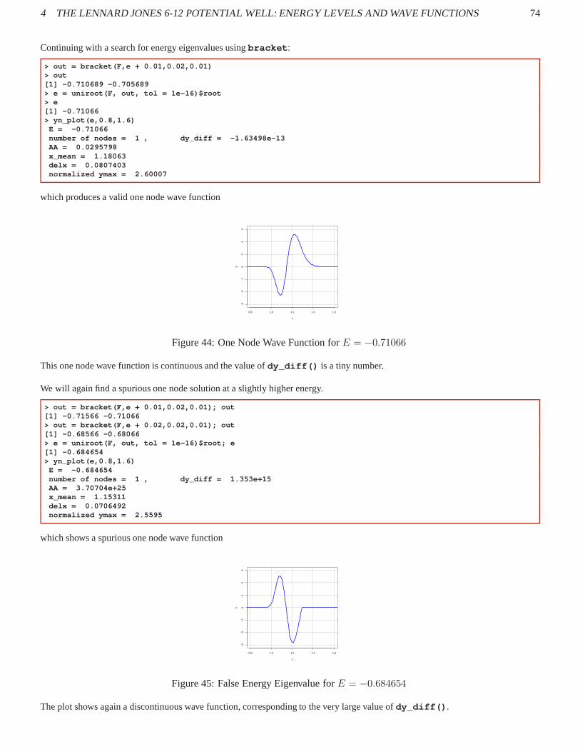
4 THE LENNARD JONES 6-12 POTENTIAL WELL: ENERGY LEVELS AND WAVE FUNCTIONS 74
Continuing with a search for energy eigenvalues usingbracket :
> out = bracket(F,e + 0.01,0.02,0.01)> out[1] -0.710689 -0.705689> e = uniroot(F, out, tol = 1e-16)$root> e[1] -0.71066> yn_plot(e,0.8,1.6)
E = -0.71066number of nodes = 1 , dy_diff = -1.63498e-13AA = 0.0295798x_mean = 1.18063delx = 0.0807403normalized ymax = 2.60007
which produces a valid one node wave function
0.8 1.0 1.2 1.4 1.6
−3
−2
−1
01
23
x
y
Figure 44: One Node Wave Function forE = −0.71066
This one node wave function is continuous and the value ofdy_diff() is a tiny number.
We will again find a spurious one node solution at a slightly higher energy.
> out = bracket(F,e + 0.01,0.02,0.01); out[1] -0.71566 -0.71066> out = bracket(F,e + 0.02,0.02,0.01); out[1] -0.68566 -0.68066> e = uniroot(F, out, tol = 1e-16)$root; e[1] -0.684654> yn_plot(e,0.8,1.6)
E = -0.684654number of nodes = 1 , dy_diff = 1.353e+15AA = 3.70704e+25x_mean = 1.15311delx = 0.0706492normalized ymax = 2.5595
which shows a spurious one node wave function
0.8 1.0 1.2 1.4 1.6
−3
−2
−1
01
23
x
y
Figure 45: False Energy Eigenvalue forE = −0.684654
The plot shows again a discontinuous wave function, corresponding to the very large value ofdy_diff() .

4 THE LENNARD JONES 6-12 POTENTIAL WELL: ENERGY LEVELS AND WAVE FUNCTIONS 75
Now that we see the pattern of valid energy eigenvalues, we can write a functionlevels(Emin,Emax,dE, Eacc) ,which usesbracket with the added filter that no sign change ofF(E) is taken seriously unless the associated wavefunction has one more node than the last energy eigenvalue found.
## levels(Emin,Emax,dE, Eacc ) returns a vector of energy le vels with## increasingly larger number of nodes in energy range (Emin , Emax).## uses F(E) to find roots, and calls wf, num_nodes() and dy_d iff() for each root found,## Uses bracket and uniroot.## The arguments (dE, Eacc) are used to call bracket, and do no t describe## the accuracy of the energy levels found.## Once a good energy e.v. is found we look for the region of## energies with one more node and search there.## Code contains an interactive continue or stop decision.
levels = function (Emin,Emax,dE, Eacc ) {rmax = 20eL = rep(NA, rmax) ## vector eL will hold energy eigenvalues f ounde = Eminnlast = -1j = 1repeat {
if (e > Emax | j > rmax) break ## exit do loopcat ("---------------- levels -------------------\n")cat (" nlast = ", nlast,"\n")cat (" Estart = ", e," dE = ", dE, "\n" )out = bracket(F,e, dE, Eacc)cat (" ea = ",out[1]," eb = ",out[2],"\n")if (out[1] == 0) {
cat (" can’t find bracket interval \n")cat (" e = ",e, "\n")break }
eroot = uniroot(F, out, tol = 1e-16)$rootcat (" eroot = ", eroot, "\n")wf(eroot)nn = num_nodes()cat (" number of nodes = ", nn, "\n")cat (" dy_diff at x = x2c is ", dy_diff(), "\n" )eL[ j ] = erootnlast = nnj = j + 1r = readline (" input c or s \n ")if (r == "s") break ## exit do loop## search for an e value greater than eb which produces## a wave function with nn + 1 nodesenext = out[2] + dErepeat {
wf(enext)if (num_nodes() > nlast) {
e = enextbreak } else enext = enext + dE } } ## end of outer repeat loop
## remove NA’s at end of vector eLeL[!is.na(eL)] }
Here is an example of use:
> EL = levels(-0.95, -0.6, 0.02,0.01)---------------- levels -------------------
nlast = -1Estart = -0.95 dE = 0.02ea = -0.9 eb = -0.895eroot = -0.896404number of nodes = 0dy_diff at x = x2c is -1.86035e-13

4 THE LENNARD JONES 6-12 POTENTIAL WELL: ENERGY LEVELS AND WAVE FUNCTIONS 76
input c or sc
---------------- levels -------------------nlast = 0Estart = -0.835 dE = 0.02ea = -0.715 eb = -0.71eroot = -0.71066number of nodes = 1dy_diff at x = x2c is -1.63498e-13input c or sc
---------------- levels -------------------nlast = 1Estart = -0.67 dE = 0.02ea = -0.555 eb = -0.55eroot = -0.551436number of nodes = 2dy_diff at x = x2c is 1.72142e-13input c or sc
> EL[1] -0.896404 -0.710660 -0.551436
We can then useyn_plot(E,xmin,xmax) to both construct the vectorsxn andyn of the normalized wave functionand make a plot. We save the normalized wave functions by assignment statements such asxn0 = xn , andyn0 = yn ,before another call toyn_plot defines the wave functions corresponding to a different energy. In the following, we donot show the plots produced by the calls toyn_plot .
> E0 = EL[1]; E0[1] -0.896404> yn_plot(E0,0.8,1.6)
E = -0.896404number of nodes = 0 , dy_diff = -1.86035e-13AA = 85.0069x_mean = 1.14069delx = 0.0455039normalized ymax = 2.97425
> xn0 = xn; fll(xn0)0.781455 2.20145 143
> yn0 = yn; fll(yn0)-3.14183e-20 0 143
We continue in this manner with the first excited state and thesecond excited state.
> E1 = EL[2]; E1[1] -0.71066> yn_plot(E1,0.8,1.6)
E = -0.71066number of nodes = 1 , dy_diff = -1.63498e-13AA = 0.0295798x_mean = 1.18063delx = 0.0807403normalized ymax = 2.60007
> xn1 = xn; fll(xn1)0.754761 2.27476 153
> yn1 = yn; fll(yn1)2.83787e-25 0 153
> E2 = EL[3]; E2[1] -0.551436> yn_plot(E2,0.8,1.6)
E = -0.551436number of nodes = 2 , dy_diff = 1.72142e-13AA = 1.24981e-05x_mean = 1.2266delx = 0.108671normalized ymax = 2.44523
> xn2 = xn; fll(xn2)0.730536 2.35054 163
> yn2 = yn; fll(yn2)0 0 163

4 THE LENNARD JONES 6-12 POTENTIAL WELL: ENERGY LEVELS AND WAVE FUNCTIONS 77
We can then combine the plots for the wave functions of these three lowest lying states.
> plot(0,type = "n",xlim = c(0.8,1.6),ylim = c(-3,3),xlab= "x",ylab="y")> lines(xn0,yn0,lwd=2,col="blue")> lines(xn1,yn1,lwd=2,col="red")> lines(xn2,yn2,lwd=2,col="green")> mygrid()> legend("bottomright",col = c("blue","red","green"),+ legend = c("E0", "E1", "E2"), lwd=2,cex=1.5)
which produces a plot of the numerical normalized wave functions describing the lowest three energy levels.
-3
-2
-1
0
1
2
3
0.8 0.9 1 1.1 1.2 1.3 1.4 1.5 1.6
y
x
E0E1E2
Figure 46: Lennard-Jones: Wave Functions for Lowest Three Energy Levels
Just for practice, we can write these three wave functions toa file in the local folder, and then restartR, read in the file contents, andmake a plot based on the file contents.
The simplest approach is to usesave(filePath,a1,a2,a3,...) , where objectsa1 , a2 , etc are object names bound to quan-tities known to R. The names and the objects bound to the namesare stored in a binary file format in the file requested (which iscreated if it does not yet exist, and overwritten if it already exists).
One can useload to load in that file into a new session, and the names and objects will then be available for use in your new Maximasession. In the following, we first save the wave function files toxy.rda . We then userm to remove knowledge of those objectsfrom the current session. We then useload to recover knowledge of those objects, which can then be usedas before, for example tomake plots and make calculations.
> save(xn0,yn0,xn1,yn1,xn2,yn2, file = "xy.rda")> rm(xn0,yn0,xn1,yn1,xn2,yn2)> fll(xn0)Error in fll(xn0) : object ’xn0’ not found> load("xy.rda")> fll(xn0)
0.781455 2.20145 143
For example, we can remake the plot of all three wave functions
> plot(0,type = "n",xlim = c(0.8,1.6),ylim = c(-3,3),xlab= "x",ylab="y")> lines(xn0,yn0,lwd=2,col="blue")> lines(xn1,yn1,lwd=2,col="red")> lines(xn2,yn2,lwd=2,col="green")> mygrid()> legend("bottomright",col = c("blue","red","green"),+ legend = c("E0", "E1", "E2"), lwd=2,cex=1.5)
and we get the same plot as above.
A proper exploration of the likely accuracy of the energy levels found in this approach would involve experimenting withthe valuesof x1decay , x2decay , and the grid sizeh. One can also modify the code so that the use of a five point symmetric formula for thefirst derivative is used, instead of the present three point symmetric formula.