computational photography: principles and...
TRANSCRIPT

Computational Photography:
Principles and Practice
HCI & Robotics
(HCI 및 로봇응용공학)
Ig-Jae Kim, Korea Institute of Science and Technology
(한국과학기술연구원 김익재)
Jaewon Kim, Korea Institute of Science and Technology
(한국과학기술연구원 김재완)
University of Science & Technology
(과학기술연합대학원대학교)

i
Preface
Computational Photography is a new research field emerging from the early 2000s, which is
at the intersection of computer vision/graphics, digital camera, signal processing, applied
optics, sensors and illumination techniques. People began focusing on this field to provide a
new direction for challenging problems in traditional computer vision and graphics. While
researchers in such domains tried to solve problems in mainly computational methods,
computational photography researchers attended to imaging methods as well as
computational ones. As a result, they could find good solutions in challenging problems by
various computations followed with optically or electronically manipulating a digital camera,
capturing images with special lighting environment and so on.
In this field researchers have been attempted to digitally capture the essence of visual
information by exploiting the synergistic combination of task-specific optics, illumination,
and sensors challenging traditional digital cameras’ limitations. Computational photography
has broad applications in aesthetic and technical photography, 3D imaging, medical imaging,
human-computer interaction, virtual/augmented reality and so on.
This book is intended for readers who are interested in algorithmic and technical aspects of
computational photography researches. I sincerely hope this book becomes an excellent guide
to lead readers to a new and amazing photography paradigm.
This book was supported from University of Science and Technology's book writing support
program for being written.

ii
Contents
1. Introduction
2. Modern Optics
2.1 Basic Components in Cameras
2.2 Imaging with a Pinhole
2.3 Lens
2.4 Exposure
2.5 Aperture
2.6 ISO
2.7 Complex Lens
3. Light Field Photography
3.1 Light Field Definition
3.2 Generation of a Refocused Photo using Light Field Recoding
3.3 Other Synthetic Effects using Light Field
3.4 Light Field Microscopy
3.5 Mask-based Light Field Camera
4. Illumination Techniques in Computational Photography
4.1 Multi-flash Camera
4.2 Descattering Technique using Illumination
4.3 Highlighted Depth-of-Field (DOF) Photography

iii
5. Cameras for HCI
5.1 Motion Capture
5.1.1 Conventional Techniques
5.1.2 Prakash: Lighting-Aware Motion Capture
5.2 Bokode: Future Barcode
6. Reconstruction Techniques
6.1 Shield Fields
6.2 Non-scanning CT

1
Chapter 1
Introduction
Since the first camera, Daguerreotype (Figure 1.1(a)), was invented in 1839, there have been
a lot of developments in terms of shape, components, functions and capturing method. Figure
1.1 shows a good comparison reflecting such huge developments between the first and a
modern camera. However, I would like to see the most significant changes have been created
in recent years through transition from a film camera to a digital camera. The transition,
maybe more accurately a revolution, doesn’t simply mean the change of an image-acquisition
way. It has rapidly changed an imaging paradigm with new challenging issues as well as a lot
of convenient functions. In spite of such huge changes, it’s ironical there is no significant
change in the shape itself as shown in figure 1.2.
(a) Daguerreotype, 1839 (b) Modern Camera, 2011
<Figure 1.1 Comparison of the first and a modern camera>

2
(a) Nikon F80 Film Camera (b) Nikon D50 Digital Camera
<Figure 1.2 Comparison of a film and a digital camera>
With the emergence of digital cameras, people easily and instantly acquire photos without
time-consuming film development process which was a necessary process in film
photography. However, such convenience brought negative matters as well. First of all,
photographic quality was critical issue in early commercialized digital cameras due to
insufficient image resolution and poor light sensitivity in image sensors. Digital camera
researchers have kept improving photographic quality to be comparable to film camera and
finally a film camera have become a historical device. However it’s still hard to say that
modern digital camera’s quality is better than film camera’s in the aspect of image resolution
and dynamic range. Researchers are constantly working to improve digital camera’s quality
and implement more convenient functions, which are shared goals in computational
photography research.
Computational photography researchers have involved in more challenging issues to break
traditional photography’s limitation. For example, digital refocusing technique controls DOF
(Depth of Field) by software processing after shooting. Probably, everyone experienced
disappointment with ill-focused photos and found there is no practical way to recover well-
focused photos by traditional methods such as deblurring functions in Photoshop. Digital
refocusing technique provides a good solution for such cases. Likewise, computational
photography researches have been broadening the borders of photography making imaginary

3
functions possible. In such stream, I convince modern cameras will be evolved to more
innovative forms.
Chapter 2
Modern Optics
2.1 Basic Components in Cameras
Let’s imagine you are making a cheapest camera. What components are indispensable for the
job? First of all, you might need a device to record light such as film or CCD/CMOS, which
are analog and digital sensors, respectively. What’s next? Do you need a lens for a cheapest
camera? What will happen if you capture a photo without a lens as Figure 2.1? You will get a
photo anyway since your film or image sensor record light somehow. However, the photo
doesn’t actually provide any visual information regarding the subject. If you are using a
digital sensor, its pixels will record meaningless light intensity and you cannot recognize the
subject’s shape in the captured photo. What’s the reason for that? As shown in Figure 2.1 (a),
every point on the subject’s surface reflects rays to all directions and they all are merged with
rays coming from different subject points onto the film or image sensor. Therefore, it’s
impossible to capture clear visible information of the subject only with a film or an image
sensor. Then, how can your cheapest camera capture the subject shape? You may need an
optical component to isolate rays coming from different subject points on a film or an image
sensor. Commercial cameras usually use lenses for this job but cheaper component is a
pinhole, which is a mere tiny hole passing incoming rays through it and blocking other rays
reaching outer region of the hole. Your camera can successfully capture the subject’s shape
with a pinhole as shown in Figure 2.1 (b).

4
<Figure 2.1 (a) Imaging without any optical components (b) Imaging with a pinhole>
2.2 Imaging with a Pinhole
Now you may have a question why commercial cameras use a lens instead of a pinhole
although a pinhole is much cheaper. Main reason is that pinhole imaging loses significant
amount of incoming rays generally causing a very dark photo compared with lens imaging
under the same exposure time. In Figure 2.1 (b), a single ray among a lot of rays reflected
from a subject point passes through an ideal pinhole while many rays pass through a lens.
The amount of incoming rays onto a film/image sensor is directly proportional to the captured
photo’s brightness.
An ideal pinhole cannot be physically manufactured in real world and actual pinholes pass
through small portion of rays per each subject point. Figure 2.3 shows how the captured
photo varies with pinhole diameter. Let’s start with imagining an extremely large pinhole.
Your photo doesn’t give the subject’s shape with it since using such pinhole is just same with
imaging by only a film/image sensor in Figure 2.1 (a). Now you use a pinhole in 2mm
Film/Image Sensor

5
diameter then your photo would look like the top-left photo in Figure 2.3. The photo is still
too blurred to recognize the subject shape due to the interference between rays coming from
different subject points. As pinhole diameter is reduced, the interference is reduced and
captured photo’s sharpness is enhanced up to a certain level. In Figure 2.3, the middle-right
photo taken with a 0.35mm diameter pinhole shows the best sharpness. If you use a much
smaller pinhole than this, will you get a much sharper photo? The answer is no as shown in
the two bottom photos. They, taken with smaller diameter pinholes, show blurred again, and
the reason for that is diffraction phenomenon.
(from Ramesh Raskar's lecture note)
<Figure 2.3 Captured photos with a pinhole according to its diameter>
Figure 2.4 shows water waves’ diffraction phenomenon and light shows similar
characteristics when passing through a very tiny area. When light experiences diffraction, it
diverges at the exit of the area in inverse proportion to the area size. Thus, the bottom-right
case with a 0.07mm diameter pinhole makes light more diverged than the bottom-left case
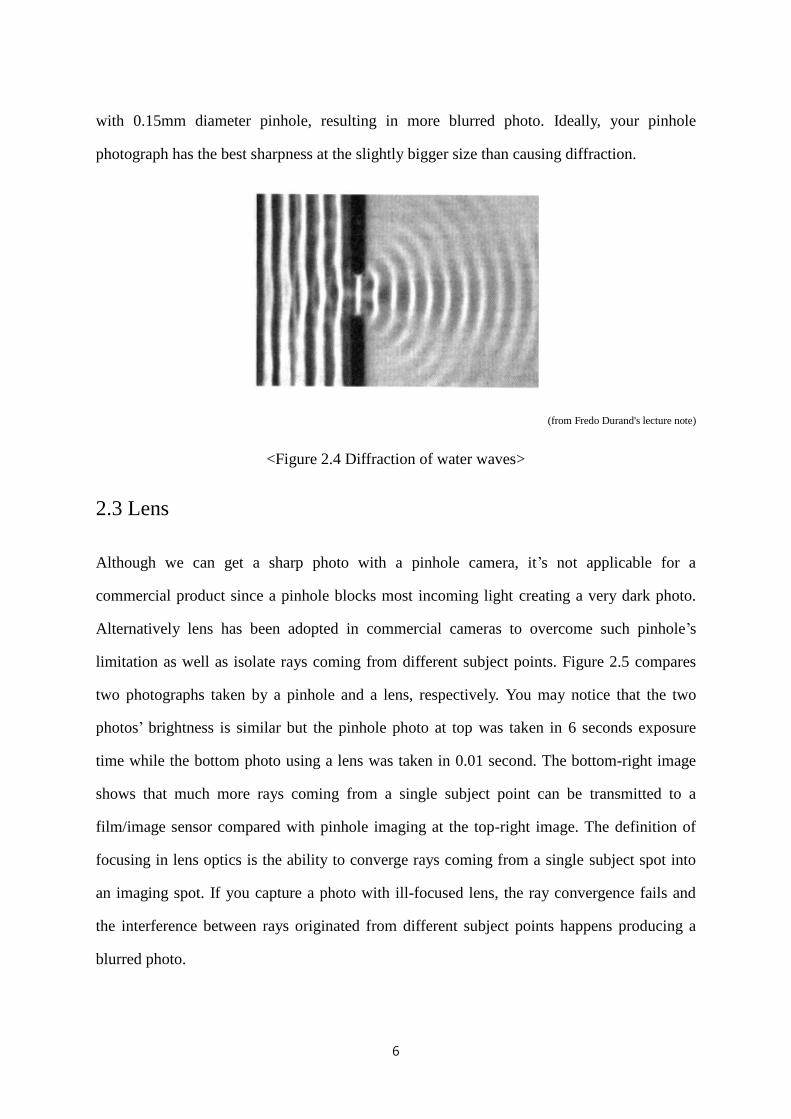
6
with 0.15mm diameter pinhole, resulting in more blurred photo. Ideally, your pinhole
photograph has the best sharpness at the slightly bigger size than causing diffraction.
(from Fredo Durand's lecture note)
<Figure 2.4 Diffraction of water waves>
2.3 Lens
Although we can get a sharp photo with a pinhole camera, it’s not applicable for a
commercial product since a pinhole blocks most incoming light creating a very dark photo.
Alternatively lens has been adopted in commercial cameras to overcome such pinhole’s
limitation as well as isolate rays coming from different subject points. Figure 2.5 compares
two photographs taken by a pinhole and a lens, respectively. You may notice that the two
photos’ brightness is similar but the pinhole photo at top was taken in 6 seconds exposure
time while the bottom photo using a lens was taken in 0.01 second. The bottom-right image
shows that much more rays coming from a single subject point can be transmitted to a
film/image sensor compared with pinhole imaging at the top-right image. The definition of
focusing in lens optics is the ability to converge rays coming from a single subject spot into
an imaging spot. If you capture a photo with ill-focused lens, the ray convergence fails and
the interference between rays originated from different subject points happens producing a
blurred photo.

7
Let’s inspect how lens transmits rays. Figure 2.6 illustrates the way in which rays are
refracted by an ideal thin lens. ‘a’ ray enters to lens in parallel direction with the optical axis
marked as a dotted line and is refracted toward the focal point of the lens. ‘b’ ray passing
through the center of lens keep moving in same direction without being refracted. All rays
coming out from the object’s point, P, are gathered in the crossing point of the two rays, P.
As an example, the third ray, ‘c’, coming out at an arbitrary angle arrives at the point, P
called as “imaging point”. Now you can easily find out the location of the imaging point for
any kind of lens given the focal point of lens by simply drawing two rays, one in parallel
direction with the optical axis and the other entering to the lens center.
<Figure 2.5 Comparison of photographs taken with pinhole and lens>

8
<Figure 2.6 A diagram for image formation with a lens>
Equation 2.1 explains a geometrical relation between focal point (f), object point distance (o)
and imaging point distance (i) from lens.
< Equation 2.1 >
There is another physical raw describing refraction in lens optics, which is Snell’s law in
Equation 2.2. When a ray penetrates a certain object such as a lens in Figure 2.7, refraction
occurs at the entry point of the object. Refraction is a physical phenomenon to explain the
change of a ray’s propagating direction at entering from a medium to a different medium. In
Figure 2.7, a ray enters to a lens at 1 incident angle and is refracted at 2 angle. The amount
of refraction is related with media’s refractive indices in Equation 2.2, n1 and n2 for the first
and second medium’s refractive index, respectively. In the case that a ray penetrates a lens in
air, like Figure 2.7, n1 and n2 indicate refractive indices of air and the lens.
i o
P
P’
f
Focal Point
a
b
c
foi
111

9
<Figure 2.7 A diagram describing Snell’s raw>
n1sin1 = n2sin2 < Equation 2.2 >
I assume you may be familiar with camera’s zoom function. Have you been curious about
how it works? When you are adjusting zoom level in your camera, actually you are changing
the focal length of lens in your camera. In photography, zoom is often called as FOV (Field of
View) which means the area of view captured in a camera. Wide FOV indicates that your
photo contains large area’s visual information and vice versa. Figure 2.8 shows the relation
between focal length and FOV. With a lens having short focal length in the figure, your
camera gets an image in the boundary of the dotted lines. While it gets an image in the
boundary of the solid lines with a lens having long focal length. Therefore, we can say there
is inverse proportional relation between focal length and FOV. Your camera lens should be set
as long focal length to achieve a shallow FOV photo, in other words a zoom-in photo. Figure
2.9 depicts the numerical relation between focal length and FOV in mm and degree,
respectively with example photos. The wide FOV photo contains wide landscape scene while
the small FOV photo does small area scene but in more detail.
12

10
<Figure 2.8 Focal length vs. FOV>
(from Fredo Durand's lecture note)
<Figure 2.9 Focal length vs. FOV in measurements>
shortfocal
length
longfocal
length
FOV
24mm
50mm
135mm
Wide FOV
Small FOV

11
2.4 Exposure
One of the most important factors in photo’s quality might be brightness. Usually, photo’s
brightness is controlled by two setting parameters, exposure time and aperture size, in a
camera and an additional parameter, ISO, for a digital camera. Exposure time means the
amount of time duration for which a film/sensor is exposed. You can imagine that longer
exposure time would make your photo brighter than shorter exposure time and vice versa.
Also, it’s straightforward to expect the effect in linear relation. For example, two times longer
exposure time would make a photo two times brighter. Usually, exposure time is set in
fraction of a second such as 1/30, 1/60, 1/125, 1/250 and etc. Long exposure time is good to
achieve a bright photo but may cause a side effect, motion blur. Motion blur is blur effect
created in a photo due to the movement of a subject or a camera while exposing. The left
photo in Figure 2.10 shows motion blur effect by the subject’s movement. Freezing motion
effect as shown in Figure 2.11 can be achieved with appropriate exposure time according to
subjects’ speed.
<Figure 2.10 Motion blurred photo (left) and sharp photo (right)>

12
(from Fredo Durand's lecture note)
<Figure 2.11 Freezing motion effect in photos with appropriate exposure times>
2.5 Aperture
Aperture indicates the diameter of lens opening, Figure 2.12 left, which controls the amount
of light passing through lens. Lens aperture is usually expressed as a fraction of a focal length
in F-number with Equation 2.3 formula (f, D and N indicate focal length, aperture diameter
and F-number, respectively.) In the formula, F-number is inversely proportional to aperture
diameter. For example given f/2 and f/4 in F-number with 50mm focal length, the aperture
diameter is 25mm and 12.5mm, respectively. F-number is typically set by following values
using a mechanism called diaphragm in Figure 2.12 right:
f/2.0, f/2.8, f/4, f/5.6, f/8, f/11, f/16, f/22, and f/32
Figure 2.13 shows different aperture sizes shaped by diaphragm.
<Figure 2.12 Lens aperture (left) and diaphragm (right)>

13
< Equation 2.3 >
<Figure 2.13 different aperture sizes controlled by diaphragm>
Aperture size is a critical factor to control photo’s brightness as exposure time. However, it
also has an important function in photography, which is the control of DOF (Depth-of-Field).
DOF is defined as a specific region where all objects are well focused. Figure 2.14 shows two
photographs for a same scene taken with different DOF settings. The left photo has a
narrower DOF where only foreground man is well focused than the right photo where the
both foreground man and background building are well focused. Such change of DOF can be
obtained by using different aperture size. The larger aperture is used, the narrower DOF is
obtained. Accordingly, the left photo in Figure 2.14 was taken with the larger aperture than
the right photo. In the left image of Figure 2.15 presenting the definition of DOF, ‘a’ location
gives the sharpest focus while ‘b’ and ‘b’ locations do slight defocus creating not a point but
a circular image for a point object in the bottom image. Such circular image is called as
‘Circle of Confusion (COC)’ and the farthest distance from the sharpest focusing location,
where COC is maximally acceptable as being focused, is defined as DOF. In the right photo
of Figure 2.15, the top and bottom pencils mark DOF.

14
(from Photography, London et al.)
<Figure 2.14 Photos with large aperture (left) and small aperture (right)>
(from Fredo Durand's lecture note)
<Figure 2.15 Definition of DOF (left) and a photo showing DOF (right)>
Now you learned aperture size is related with DOF. But what’s the mathematical relation?
The amount of change in one parameter is inversely proportional to the amount of change in
the other as shown in Figure 2.16. In the figure, if the aperture is decreased by two times, the
scene area contributing to COC is decreased by the same amount and thus DOF is doubled.
Figure 2.17 and Figure 2.18 show the relation of focusing distance vs. DOF and focal length
vs. DOF, respectively. The focusing distance is in proportional relation with DOF while focal
abb
ab

15
length is vice versa as shown in the figures.
<Figure 2.16 Aperture size vs. DOF>
<Figure 2.17 Focusing distance vs. DOF (left) and Focal length vs. DOF (right)>
In summary, DOF is proportional to focusing distance and inversely proportional to aperture
size and focal length in Equation 2.3.
< Equation 2.3 >
Until now, you learned important camera parameters, terms and their physical meanings and
relations with others. Basically you have a lot of setting options for those parameters when
DOF Focusing Distance
Aperture * Focal Length

16
shooting your camera and you need to set the best values for your target scene. Figure 2.18
shows photos taken with different aperture and exposure time values. As you see in the left
photo, large F-number (small aperture size) is good for wide DOF and requires long exposure
time to achieve enough brightness in a photo creating motion-blur artifact. The right photo
with small F-number (wide aperture size) and short exposure time is good for reduced
motion-blur artifact but background is out of focused due to reduced DOF. The middle photo
shows trade-off between motion-blur artifact and DOF.
(from Photography, London et al.)
<Figure 2.18 Photos captured with different settings of aperture and exposure time>
(Left to right setting values are (f/16, 1/8), (f/4, 1/125), and (f/2, 1/500) for F-number and
exposure time, respectively.)

17
2.6 ISO
ISO can be regarded as an electronic gain for a digital camera sensor such as CCD and
CMOS. As the most electronics gains do, it amplifies the both image signal and noise level.
ISO value linearly works for photo’s brightness and noise level. In Figure 2.19 the larger ISO
value is applied, the brighter and noisier photo is captured.
<Figure 2.19 Photos according to ISO values>
2.7 Complex Lens
If you are using DSLR (Digital Single-lens Reflex) camera, you may know there are a lot of
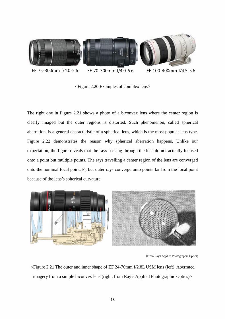
lens choices for your camera. Figure 2.20 presents a few examples of lens for a DSLR camera.
Why are there such various types of lens? The first lens’s model name is ‘EF 75-300mm
f/4.0-5.6’ where 75-300mm and f/4.0-5.6 mean the range of variable focal length and aperture
size, respectively. The both are main items but there are more in lens specifications. You need
to choose a proper one depending on your shooting scene. The left image in Figure 2.21
shows the outer and inner shape of an expensive lens, about $2,000. You see there are
multiple lenses colored in blue in the figure. You may be curious why such an expensive lens
consists of many lenses.
18
<Figure 2.20 Examples of complex lens>
The right one in Figure 2.21 shows a photo of a biconvex lens where the center region is
clearly imaged but the outer regions is distorted. Such phenomenon, called spherical
aberration, is a general characteristic of a spherical lens, which is the most popular lens type.
Figure 2.22 demonstrates the reason why spherical aberration happens. Unlike our
expectation, the figure reveals that the rays passing through the lens do not actually focused
onto a point but multiple points. The rays travelling a center region of the lens are converged
onto the nominal focal point, Fi, but outer rays converge onto points far from the focal point
because of the lens’s spherical curvature.
(From Ray's Applied Photographic Optics)
<Figure 2.21 The outer and inner shape of EF 24-70mm f/2.8L USM lens (left). Aberrated
imagery from a simple biconvex lens (right, from Ray’s Applied Photographic Optics)>
EF 70-300mm f/4.0-5.6 EF 100-400mm f/4.5-5.6EF 75-300mm f/4.0-5.6

19
<Figure 2.22 Spherical aberration>
Spherical aberration can be resolved alternatively by using aspherical lens as shown in
Figure 2.23. In the top right photo, all the rays passing through an aspherical lens are exactly
focused on a focal point and a captured photo (bottom right) with it shows that light spots are
well focused compared with those in the bottom left photo. Then, why don’t popular lenses
simply adopt aspherical lens? The reason is it’s difficult to manufacture and expensive.
Alternatively, most popular and commercial lenses are shaped in the array of spherical lenses
to compensate such imagery distortion, called as aberration in lens optics. There are several
kinds of aberration other than spherical aberration and Figure 2.24 explains chromatic
aberration which is caused by different refraction angles according to ray’s wavelength
spectrum. Generally A ray, not a single-wavelength laser, has an energy spectrum along
wavelength as shown in the top left image. The problem is that refraction is governed by
Snell’s raw in Equation 2.2 where refractive index depends on wavelength. Although a single
ray enters to a lens in the top right image of Figure 2.24, it’s refracted into separated rays
along wavelengths similarly with prism’s doing. In the figure, only three wavelength
components, B (Blue), Y (Yellow) and R (Red), are drawn for example.

20
(From Canon red book)
<Figure 2.23 Formation of spherical lens (top left) and a photo using it (bottom left).
Formation of aspherical lens (top right) and a photo using it (bottom right)>
The separated B, Y, and R rays are focused at different locations varying axially or
transversally according to the original ray’s parallel or slanted incidence respectively with
optical axis. The photos affected by the two types of chromatic aberration are shown in the
bottom. In the bottom right photo, you see color shift along horizontal direction. Additionally
lens aberration includes coma, astigmatism, curvature of field, shape distortion and so on.
Such various lens aberrations is the reason why commercial lenses come with complex lens
array in Figure 2.21.

21
<Figure 2.24 Chromatic aberration>
Axial chromatic aberration Transverse chromatic aberration

22
Chapter 3
Light Field Photography
3.1 Light Field Definition
Light field is a physical space where rays travel. A single ray can be described as Figure 3.1
with five parameters for a general 3D space movement (left) and with four parameters for a
specific movement between two planes (right), which models the case of photo shooting. The
four light field parameters in photo shooting case can be expressed as four spatial parameters,
(u, v, t, s), or two spatial and two angular parameters, (, , t, x). Now, you are ready to
understand the conversion between light field and a captured photo. Figure 3.2 top image
shows how 2D light field, the simplified version of real 4D light field, is converted to a photo
in conventional photography, where 2-dimensional ray information, (x, ) is recorded as one
dimensional information, u. You may note that the three rays coming from the subject are
equally recorded as u.
<Figure 3.1 Light field parameterization>
u
v
s
t
two-plane parameterization[Levoy and Hanrahan 1996]

23
In real photography, 4D light field information is reduced to 2D spatial information in a
captured photo. Thus, it can be said that photo shooting is a process to lose higher
dimensional information in light field. Unfortunately, such information loss has put
fundamental limitations in photography history. A representative limitation might be the
impossibility of refocused photo. You may have a lot of experience that your photo’s target
subjects are mis-focused and there is no way to recover a well-focused photo but re-shooting.
In computer vision, many techniques like sharping operation have been widely explored but
such techniques couldn’t provide a comparable result with a re-shooted photo since the
restoration of higher dimensional information from already lost information is inherently an
ill-posed problem. If the limitation is originated from the information-losing process, how
about recording the whole light field without losing the information? The figure 3.2 bottom
image exactly explains the idea, where the two-dimensional light field information is fully
recorded as 2D spatial information in photosensor by the help of microlens array.
<Figure 3.2 Light field conversion into a photo>

24
With the fully recoded light field, we can identify each ray’s information coming from
different subjects and conceptually a refocused photo can be generated by using the
distinguished ray information for target and background objects. The detail process to
generate a refocused photo is covered in the next chapter. Recently, many researchers are
working on applications associated with light field information and some are on its recoding
methods. Representative applications and recoding methods are dealt in following sections.
3.2 Generation of a Refocused Photo using Light Field Recoding
One of light field applications with huge attention is refocused photography. Figure 3.3
shows the technique’s results where each photograph shows different DOFs. Those five
photographs are generated from a single captured photo with only computation, which means
photograph’s focus is adjustable after shooting according to a user’s intention. In the first
photo only the front woman is well focused, in the second photo the second front man is, and
so on. Therefore, although your original camera DOF missed the target subject in a captured
photo, you can generate a well-focused photo for the subject by computation with applying
the technique. Now let’s find out how to implement this technique.
(from Stanford Tech Report CTSR 2005-02)
<Figure 3.3 Refocused results along various DOFs>

25
Figure 3.4 shows one of the refocusing cameras, Stanford Plenoptic camera1, which has been
implemented by Marc Levoy’s research group. The only thing you need to modify the camera
is inserting a microlens array in front of the image sensor. The top photos show the camera
which was used for their experiments and the exposed image sensor with disassembling the
camera. The bottom-left photo represents the microlens array which is the key element to
record light field and the bottom-right one is a zoom-in photo for the small region of it. The
microlens array consists of 292292 tiny lenses in 125 m square-sided shape. Each
microlens plays a role to diverse the individual incoming rays to different image sensor space,
as shown in the bottom image of Figure 3.2.
(from Stanford Tech Report CTSR 2005-02)
<Figure 3.4 Stanford Light Field (Plenoptic) Camera>
1 NG, R., LEVOY, M., BREDIF, M.,DUVAL, M.,HOROWITZ, G., AND HANRAHAN, P. 2004. Light field photography with a hand-held
plenoptic camera. Tech. rep, Stanford University.
Contax medium format camera Kodak 16-megapixel sensor
Adaptive Optics microlens array 125μ square-sided microlenses
(292x292 microlenses)

26
The left photo of Figure 3.5 shows a raw photo captured by Stanford Plenoptic camera shown
in Figure 3.4 in 40004000 pixel resolution. (a), (b) and (c) are zoom-in photos for the
corresponding regions marked in (d), a small version of the raw photo. In (a), (b) and (c), you
see small circular regions which are images formed by microlenses. Basically the raw photo
provides 2D spatial information and each microlens image does additional 2D angular
information. Thus, you can assume that the raw photo contains 4D light field information.
Since the raw photo’s resolution is 40004000 and it includes 292292 microlens images
with neither pixel gap nor overlapping between them, each microlens image has 1414 pixel
resolution by simple division.
(from Stanford Tech Report CTSR 2005-02)
<Figure 3.5 A raw photo captured by Stanford Plenoptic camera>
Figure 3.6 explains how to process the raw light field photo to generate digitally refocused
images like Figure 3.3. Let’s assume that ‘b’ position in the figure is our aiming focal plane in
Raw light field photo (4000x4000 pixels)
(a) (b)
(c) (d)

27
the refocused photo. Then, we need to trace where the ray information consisting ‘b’ plane is
located in the capture light field photo. Interestingly, it’s dispersed in different microlens
images as shown in the right side of the figure. As a result, a refocused photo for ‘b’ plane
can be generated by retrieving the dispersed ray information in green regions. Refocused
photos for different focal planes are generated by same logic.
<Figure 3.6 Image processing concept for refocusing technique>
3.3 Other Synthetic Effects using Light Field
3.3.1 Synthetic Aperture Photography
Figure 3.7 shows relation between aperture size of main lens and microlens image. Large
aperture lens allows incoming rays at wide angles increasing angular dimension in microlens
image. In other words, the size of microlens image is proportional to the main lens’s aperture
size as shown in the figure. Basically, more angular information is desirable in most cases
however overlapping between microlens images as the bottom figure must be avoided. As a
design concept in implementing a light field camera, you need to choose an optimum aperture
size for main lens, which gives the largest microlens images with no overlapping as f/4
aperture case in Figure 3.7.
Σa b

28
(from Stanford Tech Report CTSR 2005-02)
<Figure 3.7 Variation in microlens images according to main lens’s aperture size>
How can you utilize the relation between main lens’s aperture size and microlens image to
implement synthetic aperture photography? Figure 3.8 top represents light field imaging with
main lens’s full aperture. Averaging each microlens image gives a normal photograph
captured with the main lens. Now your mission is to generate a synthetic photo with smaller
main lens aperture by processing a light field raw photo as shown in the top figure. You can
simply perform this job by averaging small circular region pixels, marked as a green circle in
the bottom-right figure, in each microlens image. The circular region size is proportional to
your synthetic aperture size. Such synthetic aperture photography has a major benefit in DOF
extension.

29
<Figure 3.8 Image processing concept for synthetic stopping-down effect>
Figure 3.9 demonstrates such effect comparing conventional and synthetic aperture
photographs. In the left photo captured with f/4 lens, the woman’s face in the red rectangle is
out-of-focused since she is out of the lens’s DOF. The middle photo shows the same woman’s
face is well focused due to extended DOF with f/22 lens but noisy for the decreased amount
of photons. The right photo is a processed result for synthetic stopping-down using light field
photograph. In the photo, as you can see, the woman’s face is well-focused and much less
noisy than the middle photo. In summary, you can achieve the extension of DOF as well as
good SNR in synthetic aperture photograph.
Σ
Σ

30
(from Stanford Tech Report CTSR 2005-02)
<Figure 3.9 DOF extension by light field photography>
3.3.2 Synthetic View Photography
A conventional photo contains only single view information and we cannot get different view
information from it. What if there is a photograph with which we can see different views of
subjects? Such photograph would be much more informative and useful than a conventional
one. Light field camera can be utilized to provide such a magical photograph. Collecting
averaged pixels from a center region of each microlens image generates a reference view
photograph which is synthetically same with a conventional photo. (Figure 3.10 top) If we
collect averaged pixels from a bottom region of each microlens image (Figure 3.10 bottom-
right), synthetic bottom view photograph is generated. Likewise, arbitrary view photos can be
acquired from a light field photograph. Figure 3.11 shows synthetic top and bottom view
photos where vertical parallax is clearly observed.
conventional photograph,main lens at f / 22
conventional photograph,main lens at f / 4
light field, main lens at f / 4,after all-focus algorithm
[Agarwala 2004]

31
<Figure 3.10 Image processing concept for synthetic view effect>
<Figure 3.11 Synthetic top and bottom view images created from a light field photograph>
Σ
Σ

32
3.4 Light Field Microscopy
Marc Levoy’s group at Stanford presented light field microscopy system2 in 2006. They
implemented the system by attaching a microlens array and digital camera to a conventional
microscope as shown in Figure 3.12. You can compare differences between a conventional
and light field microscope in Figure 3.13 where an imaging sensor substitutes for human eyes
and eyepiece lens is replaced by a microlens array. The overall scheme is similar with
Stanford Plenoptic camera covered in the previous section. Rays reflected from the specimen
are focused onto the intermediate image plane where the microlens array allocates the
incident rays into the sensor pixels.
(from LEVOY, M.,NG, R.,ADAMS, A., FOOTER, M., AND HOROWITZ,M. 2006. Light field microscopy. ACM Trans. Graph. 22, 2)
<Figure 3.12 Marc Levoy group’s light field microscopy system>
2 LEVOY, M.,NG, R.,ADAMS, A., FOOTER, M., AND HOROWITZ,M. 2006. Light field microscopy. ACM Trans. Graph. 22, 2
microlensarray

33
Figure 3.14 shows a captured photo for a biological specimen by the light field microscope.
In the right close-up photo, microlens images containing 4-dimensional light field
information in circular shape are clearly shown and the information can be used to provide
various visualization effects.
(a) a conventional microscope (b) a light field microscope
<Figure 3.13 Comparison between a conventional and a light field microscope>
(from LEVOY, M.,NG, R.,ADAMS, A., FOOTER, M., AND HOROWITZ,M. 2006. Light field microscopy. ACM Trans. Graph. 22, 2)
<Figure 3.14 Light field microscope photo (left) and its close-up photo (right) >
objective
specimen
intermediate
image plane
eyepiece
sensor
microlens
array

34
Figure 3.15 demonstrates that light field microscope creates various view images for the
specimen by user interaction from a single captured photo. This is very useful function in
microscopy since it’s very troublesome task to change a specimen’s pose and re-setup
microscopic conditions such as lens focusing for observing different views of the specimen.
Plus, light field microscope can generate a photo focused at an arbitrary focal plane as shown
in Figure 3.16. In the figure, the specimen’s specific depth plane is focused and other plans
are out-of-focused, which can be achieved by a similar processing with refocusing technique
in previous section.
<Figure 3.15 Specimen’s view change by user interaction>
(from left to right, left-side, front and right-side view)
<Figure 3.16 Specimen’s focal plane change>
(from left to right, left-side, front and right-side view)

35
Possessing arbitrary 2D view information about an object means that 3D reconstruction for
the object’s shape is possibly achieved. Figure 3.17 shows the 3D reconstruction results
which are rendered using the synthetic view images presented in Figure 3.15. That’s a very
powerful feature of light field microscopy with providing 3D shape information for a
specimen from a single photo. In summary, users can be benefited in understanding
specimen’s 3D shape and detailed observance for a specific part of it with using light field
microscopy.
<Figure 3.17 3D reconstruction result for a specimen using light field microscope>
3.5 Mask-based Light Field Camera
Section 3.3 described Stanford Plenoptic camera which records 4D light field information
using a microlens array. Needless to say, a microlens array is an effective component to
capture light field but it’s not cheap. Stanford’s microlens array costs thousands US dollars
for a master model and hundreds US dollars for a copy. So, some researchers proposed a
mask-based light field camera3 in cheap cost as shown in Figure 3.18. In the camera, a mask
with attenuating pattern is adopted instead of a microlens array in Stanford Plenoptic camera.
3 Veeraraghavan, A., Raskar, R., Agrawal, A., Mohan, A., Tumblin, J.: Mask enhanced cameras for heterodyned light fields and coded
aperture refocusing. ACM SIGGRAPH 2007

36
The mask plays an exactly same role, transmitting 2D angular information, with a microlens
array at same place near an image sensor. In Section 2.2, we learned that pinhole’s role in
image formation is same to lens’s. Basically a pinhole mask in Figure 3.19 left can be
adopted for a microlens array. However, pinhole’s limitation, attenuating incoming photons,
still holds. Alternatively, cosine (Figure 3.18 bottom-left) or tiled-MURA mask (Figure 3.19
right) can be used to implement a mask-based light field camera.
<Figure 3.18 Mask-based light field camera>
<Figure 3.19 Pinhole and tiled-MURA mask>
MaskSensor
Cosine Mask

37
The two masks consist of repetitive patterns and each pattern region can be regarded as a
single microlens. However, they have a distinct feature in process to transmit incoming rays
comparing with a microlens array. While a microlens array spatially allocates 4D light field
into image sensor, a cosine or tiled-MURA mask do in frequency domain. A captured photo
with a cosine mask in Figure 3.20 looks similar with Stanford Plenoptic camera photo in
Figure 3.5 however 4D light field information cannot be extracted by pixel-wise operation
but frequency domain operation. Figure 3.21 shows how light field information is transmitted
by such masks. In the figure, light field consists of 2-dimensional parameters, x and for
spatial and angular information, respectively. Figure (a) explains that light field in frequency
domain is vertically modulated along axis when the mask is located at aperture plane.
Whereas, when the mask is between aperture and sensor plane in Figure (b), light field is
modulated along a slanted line at angle from the horizontal axis. is given by the ratio of
‘d’, distance between mask and sensor plane, and ‘v’, distance between aperture and sensor
plane.
<Figure 3.20 A captured photo with a cosine mask>
Encoding due to Mask

38
Such modulation is a key process to transmit light field into image sensor in frequency
domain as shown in Figure 3.22. Figure (a) represents a normal imaging process without a
mask. Original light field in frequency domain, fx and f, is captured recording only fx
information marked as the red-dot rectangle. Figure (b) represents the case the light field is
modulated by a mask. In the same manner, image sensor only records fx information
surrounded by the red-dot rectangle but actually it includes replicas of f information. The
five small boxes in the red-dot rectangle match with original light field’s boxes, which means
that light field can be recorded in fx domain without loss.
(a) when a mask at aperture position (b) when a mask between aperture and sensor
<Figure 3.21 Light field modulation by a cosine mask.>
x-planex
(a)
(b)

39
Figure 3.23 conceptually shows a process to recover the original light field from the recorded
sensor signals. In the figure, the dispersed light field information regarding fx and f is
rearranged by demodulation process.
(a) Lost light field recording without a mask (b) Full light field recording by mask
modulation
<Figure 3.22 Image sensor’s capturing for light field>
<Figure 3.23 Light field recovering through demodulation process>

40
Figure 3.24 shows a traditional capturing case for two plane objects. 2D Light field from the
objects and its FFT image are shown in the x- and fx-f space, respectively. That’s our target
information for capturing but unfortunately our sensor captures only x-dimensional
information in the bottom-right image. In mask-based light field capturing, a sensor image
and its FFT image for the same objects are shown in the top-right of Figure 3.25. Note the
ripple signal in the sensor image which represents the modulated signal by a mask. The
modulated light field FFT clearly shows light field replicas along a slanted line and the sensor
FFT represents its 1D signal along the sensor slice parallel to x-axis.
<Figure 3.24 In traditional capturing, an example of a sensor image and its Fourier transform
image>
<Figure 3.25 In mask-based light field capturing, an example to recover light field from a
modulated sensor image>
Modulated light field FFT

41
Since the sensor FFT image includes slices of the original light field, rearranging them in
FFT domain gives the FFT signal of the light field and in turn light field in spatial domain by
inverse Fourier transform. Figure 3.26 compares a traditional photo and its FFT image with a
mask-based light field camera photo and its FFT image. The FFT image of light field camera
photo contains slices of the original light field in the bottom-right image. The light field FFT
signal can be reconstructed by rearranging them in 4D frequency domain and the original
light field in spatial domain is acquired by its 4D inverse Fourier transform.
<Figure 3.26 A traditional photo and its FFT image (top) vs. Mask-based light field camera
photo and its FFT image (bottom)>
2D FFT
Traditional Camera Photo Magnitude of 2D FFT
Mask-based LF Camera Photo
2D FFT
Magnitude of 2D FFT

42
Figure 3.27 compares a conventional photo with refocused images acquired by a mask-based
light field camera. The original photo (a) has DOF for middle parts, which is similar with
refocused image for middle parts in the figure (b). Contrastively, the refocused images in (c)
and (d) show better focused images than the original photo for far and close parts,
respectively.
(a) Raw sensor photo (b) Refocused image for middle parts
(c) Refocused image for far parts (d) Refocused image for close parts
<Figure 3.27 Raw photo vs. refocused images acquired by a mask-based light field camera>
43
Chapter 4
Illumination Techniques in Computational
Photography
Ambient light is a critical factor in photography since photographic subjects can be
considered as reflectors sensitively reacting to it. Professional photographers sometimes use
specialized lighting system to capture good photographs and general users often take pictures
with bursting a flash in dark environment. It’s true that photographic lighting system was
commonly considered as an accessorial tool for better photos. But recently many researchers
are focusing on its usages to achieve additional information or newer visualization effects in
computational photography field. Synthetic Lighting photography in 1992, Figure 4.1,
presented by Paul Haeberli was an initiative work in such stream. In the work, synthetic
lighting photo with beautiful colors as shown in the boom is generated from white
illumination. The first row photos are captured with white illumination at different directions
and then different color channel is extracted from each photo in the second row. The final
synthetic lighting result is generated by mixing the color channels. Although the processing is
very simple, the result gives a beautiful and interesting photo which cannot be obtained by a
conventional light. In following sections, more interesting techniques are described.

44
<Figure 4.1 Synthetic light photography>
4.1 Multi-flash Camera
A conventional camera has only one flash to make the photo scene bright. While, Raskar et al.
presented a four-flash camera as shown in Figure 4.2, called Multi-flash camera4. Now, let’s
begin with the background behind of the camera’s invention. See photos in Figure 4.3.
What’s your first feeling on them? You feel the objects in the photos are very complicated so
it’s difficult to recognize any parts. That maybe the reason why car manuals use drawings as
4 RASKAR, R., TAN, K.-H., FERIS, R., YU, J., AND TURK, M. 2004. Nonphotorealistic camera: depth edge detection and stylized
rendering using multi-flash imaging. ACM Trans. Graph. 23, 3, 679–688.
Photo at first directional lighting Photo at second directional lighting Photo at third directional lighting
Red channel extraction Green channel extraction Blue channel extraction
Synthetic lighting result

45
shown in Figure 4.4 instead of real photos in figure 4.3. Sometimes raw photos makes viewer
complicated and are less effective to convey shape information. However, drawings in Figure
4.4 cost more than photos because they should be drawn by artists. What if there is a magical
camera to produce such drawing? Multi-flash camera in Figure 4.2 is intended for the
purpose.
<Figure 4.2 Multi-flash camera system>
<Figure 4.3 Complicated scene photos>

46
Figure 4.5 compares a raw photo and its Canny edges with Multi-flash camera image. The
figure demonstrates the unique feature of Multi-flash camera distinguished from general
edges such as Canny edges shown in the middle figure, which is the extraction of depth edges
for front objects. In the input photo, a hand is located at the front of an intricately textured
object. General edge detection algorithms detect pixels where their intensities rapidly change.
<Figure 4.4 Drawings in car manuals>
<Figure 4.5 Input photo vs. Canny edges vs. Multi-flash camera image>
Input Photo Canny Edges Multi-flash camera image

47
Accordingly, the Canny edge result in the middle reflects all the complicated edges in the
background texture. While, Multi-flash camera detects pixels where an object’ depth position
rapidly changes, which is the definition of depth edges. How can Multi-flash camera detect
depth edges with a regular 2D image sensor? Four flashes in Multi-flash camera are the key
part for the function.
<Figure 4.6 Photos captured with four flashes in Multi-flash camera>
<Figure 4.7 Depth edges from Multi-flash camera>

48
Figure 4.6 shows four photos captured with one of the four flashes in Multi-flash camera.
Since the four flashes illuminate at left, right, top and bottom directions as shown in Figure
4.2, Figure 4.6 photos are captured with corresponding directional lights. The top-left in
Figure 4.6 is captured with left illumination so shadow is created at right direction. Likewise
photos with right, top and bottom illumination contains shadows at opposite directions with
illumination. From the four photos, we have full-directional shadow for the object and depth
edges are located at the intersectional points between the object and its shadow. Processing
steps in Figure 4.8 are exactly intended to detect such points. The processing starts with
capturing four directional shadow images with Multi-flash camera. Next step is generating a
Max image of which pixels have same intensity values with maximum pixels among the four
input images at each pixel position. The Max image represents a shadow-free image. The four
input images are divided by Max image, which is called a normalization process. Normalized
images have enhanced shadow signals in low pixel values as shown in the second column of
Figure 4.8 since non-shadow region becomes close to 1 by division.
<Figure 4.8 Processing steps in depth edge detection>
Normalized
Left / Max
Right / Max
Left Flash
Right Flash
Input depth edgesLine-by-line
searching

49
Next step is detecting depth edge pixels by line-by-line searching as shown in the third
column. Note that searching direction depends on the shadow direction. For example, in a left
flash image, shadows are created in the right-side of the object and the searching direction is
left-to-right in the top row images of Figure 4.8. In the same logic, a right flash image in the
bottom row is processed by right-to-left searching. Depth edges are located in the negative
transition points at line-by-line searching (the third column). Final depth edge image is
generated by collecting all depth edge pixels from given four input images in the fourth
column. Figure 4.9 shows a depth edge result for complicated mechanical parts with four
input flash photos and Max image.
<Figure 4.9 Depth edge image from four flash photos>

50
Figure 4.10 compares a depth edge image by Multi-flash camera with a conventional Canny
edge image. The depth edge image much more effectively conveys the complex objects’
shape information than the Canny edge image. Additionally a depth edge image can be
combined with pseudo color to provide better visibility as shown in the top-right of Figure
4.10. The pseudo color information is sampled from the original photo’s color information.
<Figure 4.10 Depth edge image vs. Canny edge image>
Canny Intensity Edge Detection
Our Method
Photo Result

51
Depth edge image by Multi-flash camera works well for various types of complex objects
including flowers and even hairs in Figure 4.11.
<Figure 4.11 Depth edge results for complex objects>

52
4.2 Descattering Technique using Illumination
In our environment, various kinds of reflections happen at every time. Actually, seeing
objects means the objects are reflecting light. In computer vision and graphics fields, such
reflections are often categorized into two groups, direct and global reflections. Researchers
have been tried to separate those two in their sensed light signals because they have different
characteristics and information. However, the separation of direct and global components of
incident light has been a challenging topic due to the complex behavior of reflection
including inter-reflection, subsurface scattering, volumetric reflection, diffusion, and so on.
These complex characteristics are one of the main factors hindering an analytical solution for
the separation of direct-global reflection. For this reason, active coding methods have been
proposed by Nayar et al5. They projected high-frequency patterns onto a reflective scene to
achieve accurate and robust separation. Narasimhan et al6. used structured light to estimate
the 3-D shape of objects in scattering media, including diluted suspensions. Atcheson et al7.
estimated the 3-D shape of non-stationary gas flows. In many previous approaches, scattering
scenes composed of low density materials (eg. smoke, liquid, and powder) have been
explored where single scattering mode is dominant. However, general scene is not modeled
by just single scattering but multiple scattering. A computational photography approach to
tackle the problem in multiple scattering case was introduced by Jaewon Kim et al8. based on
angular filtering with a microlens array. Figure 4.12 presents their optical setup and its
5 NAYAR, S., KRICHNAN, G., GROSSBERG, M., AND RASKAR, R. 2006. Fast separation of direct and global components of a scene
using high frequency illumination. ACM Trans. Graph. 25, 3, 935-943.
6 Narasimhan, S.G., Nayar, S.K., Sun, B., Koppal, S.J.: Structured light in scattering media. In: Proc. IEEE ICCV, vol. 1, pp. 420–427
(2005)
7 Atcheson, B., Ihrke, I., Heidrich, W., Tevs, A., Bradley, D., Magnor, M., Seidel, H.P.: Time-resolved 3D capture of non-stationary gas
flows. In: ACM TOG (2008)
8 KIM, J., LANMAN, D., MUKAIGAWA, Y., AND RASKAR, R. 2010. Descattering transmission via angular filtering. In Proceedings of
the European Conference on Computer Vision (ECCV’10). Lecture Notes in Computer Science, vol. 6311. Springer, 86-99.

53
schematic diagram. In the figure (a), they placed multiple scattering media consisting of
milky water and a target object between a LED light and a camera. Such milky water creates
multiple scattering so the target object inside of the milky water tank is barely recognizable.
The figure (b) shows the process to create multiple scattering in participating media such as
milky water. Rays emitted from a LED in blur color travels through the media where particles
scatter the rays at irregular directions in red color. Scattered rays keep scattered again by
other particles, which creates multiple scattering. This research tried to separate the original
rays, direct rays in blue, emitted from a LED from the scattered rays in red using a pinhole or
microlens array placed in front of a camera. Figure 4.13 explains how such pinhole or
microlens array can be used to separate direct and scattered rays. In the figure (a), direct rays
are simply mixed in a captured photo without such optical components while there exist two
regions in pinhole or microlens array imaging as shown in the figure (b). One is ‘pure
scattered’ region and the other is ‘mixed direct-scattered’ region. Such two regions’ creation
is originated from difference in ray’s incident angle. Direct rays emitted from a LED have
limited incidence angle at imaging through a pinhole or microlens. In the figure (b), the direct
rays’ incidence angle range is bounded by mixed direct-scattered region. While, scattered
rays have much wider range of incidence angle than direct rays so it includes pure scattered
region as well as mixed direct-scattered region. The important fact is that scattered rays’
imaging contribution can be estimated from pure scattered region.
<Figure 4.12 Optical setup for descattering based on angular filtering>

54
Once scattered rays’ values are obtained, direct rays’ values can be computed by subtracting
the scattered rays’ values from mixed direct-scattered values. Figure 4.14 demonstrates such
computation process.
<Figure 4.13 Imaging of multiple scattering scene without (a) and with (b) a microlens or
pinhole array>
<Figure 4.14 Computation strategy for separation of direct and scattered values>

55
The figure (a) is one dimensional intensity profile in a pinhole or microlens image without
scattering. The profile shows a sharp peak contributed by pure direct rays while profile in the
figure (b) shows a gradual intensity change due to scattered rays’ contribution. Note that still
direct rays’ contribution is limited in the same ‘direct region’ of the figure (a), which becomes
‘mixed direct & scattered region’ in the figure (b). In the figure (c), unknown scattered values
for ‘mixed direct & scattered region’ are estimated from known scattered values in ‘pure
scattered region’ and then direct values for ‘mixed direct & scattered region’ are calculated by
subtracting the estimated scattered values from the original ‘mixed direct & scattered region’
values. By repeating this process for all pinhole or microlens images, scattered-only and
direct-only images are generated in Figure 4.15. From left to right column, milky water’s
concentration increases making more scattering. Although the horse-shape object in milky
water tank looks unclear with increased concentration, the direct-only images provide clear
shape information for the object since scattered rays’ contribution to make the object unclear
is eliminated.
<Figure 4.15 Direct-only and scattered-only images>
Object in milky
water tank

56
Figure 4.16 shows SNR (Signal to Noise Ratio) comparisons for the red line in the top-left of
Figure 4.15. In normal photos, the signal is not distinguishable for high concentration case
(Figure 4.16 (a)) while it does in direct-only image (b). As shown in the graph (d), the
signal’s SNR is rapidly decreased with the incense of milky water concentration while it’s
slowly decreased in direct-only image.
<Figure 4.16 SNR comparisons in a normal photo vs. direct-only image>

57
This research can be applied to various media including shallow parts of human body such as
fingers. Figure 4.17 shows near-infrared imaging setup to visualize human finger veins. Near-
infrared is widely used for vein visualization since hemoglobin in veins absorbs the light
making veins dark in an infrared image as shown in Figure 4.17 (b). To capture an infrared
image, they attached IR-pass filter to a camera with removing IR-cut filter inside of the
camera in Figure 4.17 (a). Infrared light emitted from the IR LED penetrates a finger
allowing a finger vein image to the camera in the figure (b). However, vein shape in the
image is still vague. So, direct-only image can be applied to provide better visibility for the
finger veins as shown in the figure (c).
<Figure 4.17 Direct-scattered separation images for a human finger
using infrared imaging setup>

58
Finger vein shape can be utilized for personal identification or authentication as finger print
because each person has different finger vein shape. Already commercial products using
finger veins for personal identification have been presented as shown in Figure 4.18. Finger
vein is regarded as a safer biometrics than finger print so there were attempts to use finger
vein-based identification for banking service. Direct-scattered separation technique can be
applied to those devices to improve the accuracy by offering a clearer finger vein image.
<Figure 4.18 Examples of finger vein authentication devices>
<Hitachi> <Sony>
Finger vein recognition for personal ID
Personal authentication and security
59
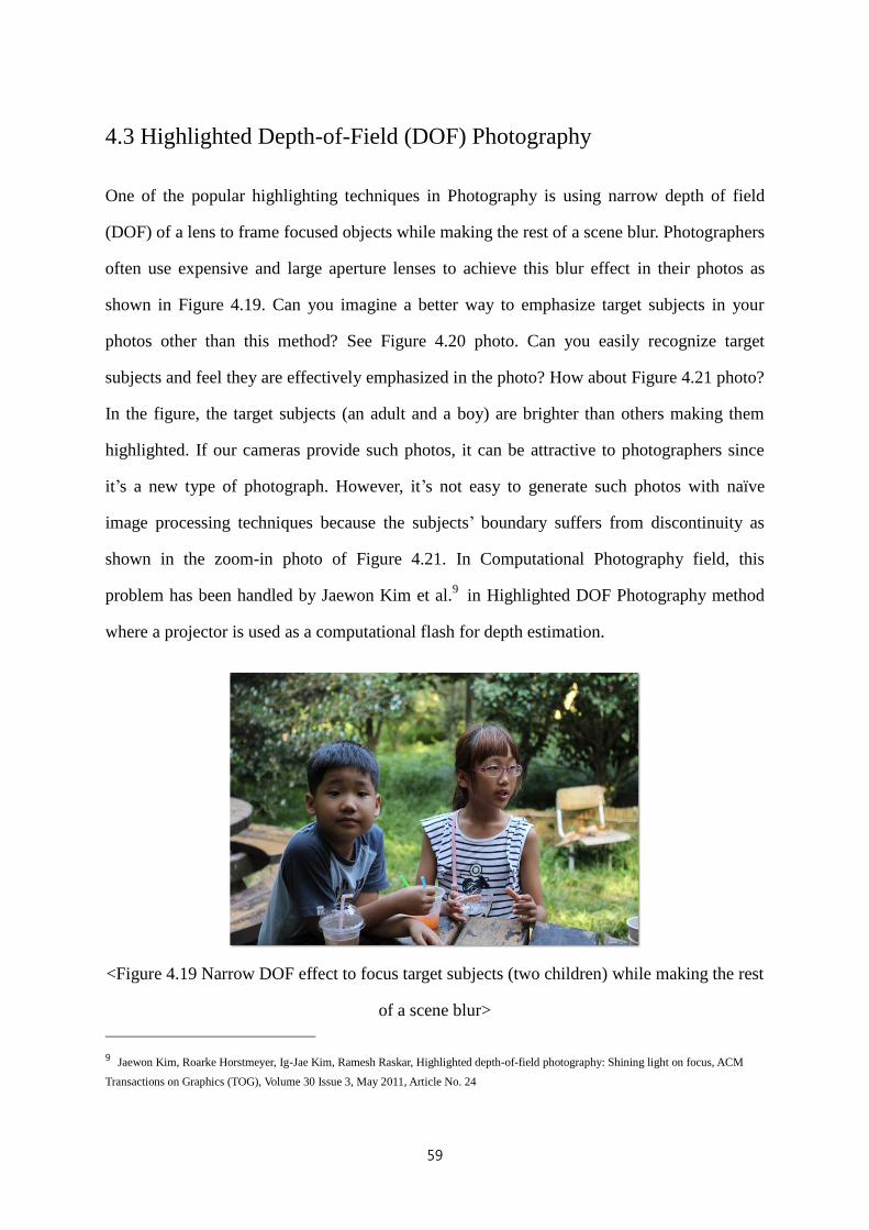
4.3 Highlighted Depth-of-Field (DOF) Photography
One of the popular highlighting techniques in Photography is using narrow depth of field
(DOF) of a lens to frame focused objects while making the rest of a scene blur. Photographers
often use expensive and large aperture lenses to achieve this blur effect in their photos as
shown in Figure 4.19. Can you imagine a better way to emphasize target subjects in your
photos other than this method? See Figure 4.20 photo. Can you easily recognize target
subjects and feel they are effectively emphasized in the photo? How about Figure 4.21 photo?
In the figure, the target subjects (an adult and a boy) are brighter than others making them
highlighted. If our cameras provide such photos, it can be attractive to photographers since
it’s a new type of photograph. However, it’s not easy to generate such photos with naïve
image processing techniques because the subjects’ boundary suffers from discontinuity as
shown in the zoom-in photo of Figure 4.21. In Computational Photography field, this
problem has been handled by Jaewon Kim et al.9 in Highlighted DOF Photography method
where a projector is used as a computational flash for depth estimation.
<Figure 4.19 Narrow DOF effect to focus target subjects (two children) while making the rest
of a scene blur>
9 Jaewon Kim, Roarke Horstmeyer, Ig-Jae Kim, Ramesh Raskar, Highlighted depth-of-field photography: Shining light on focus, ACM
Transactions on Graphics (TOG), Volume 30 Issue 3, May 2011, Article No. 24

60
(from activities4kids.com.au)
<Figure 4.20 Ineffectiveness of defocus-based highlighting photography>
<Figure 4.21 Brightness-based highlighting photography>

61
Figure 4.22 shows the basic idea for their method using intensity drop in the light reflected
from out-of-focused objects. When a spotlight source illuminates a focused object, the
brightness of the spot is high and its size is small in a captured photo in the top of Figure 4.22.
While, in the case that a spotlight source illuminates an out-of-focused object, the brightness
of the spot is low since the light energy is dispersed in large area as shown in the bottom of
Figure 4.22.
<Figure 4.22 Basic concepts for highlighted DOF photography. Light reflected from a
focused object has high intensity (top) while light reflected from an out-of-focused object has
low intensity (bottom)>
Point light Camera
In-focus
Out-of-focusPhoto
Spot is small and intensity is high
Scene
Point light Camera
Spot is large and intensity is low
In-focus
Out-of-focusPhoto
Scene

62
Therefore, a highlighted DOF photo can be simply generated by scanning a spotlight,
capturing photos at each spotlight position and collecting spot pixels in the captured photos in
Figure 4.23. However, such method takes so much time and requires capturing huge number
of photos. Alternatively, dot-pattern projection method has been presented in Figure 4.24.
Spotlight scanning and capturing multiple photos can be substituted by a dot-pattern
projection and a single-shot capture as the figure demonstrates.
<Figure 4.23 Generation of highlighted DOF photo by spotlight scanning>
<Figure 4.24 Generation of highlighted DOF photo by dot-pattern projection>
Point light Camera
In focus
Out-of-focus
Highlighted DOF Photo
Dot Pattern Projection
Projector
Camera
Photo Photo
Spotlight Scanning
Point light source Camera
In focus
Out-of- focus
Point light source Camera
In focus
Out-of- focus

63
Bright regions in dot-pattern is regarded as a spotlight so in a processing step pixels for the
bright regions are collected to create a highlighted DOF photo as shown in Figure 4.25. You
see bright regions in the capture photo (left side) and the middle image is the processed
highlighted DOF photo where the focused green crayon looks brighter than others in
comparison with the conventional photo (right side). However, this method has a
disadvantage in reduced resolution as shown in the characters of the highlighted DOF photo.
<Figure 4.25 A highlighted DOF photo vs. a conventional photo>
<Figure 4.26 Dot-pattern shift and multi-shot capturing method>
Highlighted DOF Photowith reduced resolution
Conventional PhotoCaptured Photo
Dot pattern
Shift
Captured 9 photos
Highlighted DOF Photo
Max. pixel in each pixel coordinate

64
To overcome the limitation, they proposed the second method, called multishot method, by
shifting a dot-pattern and capturing multiple photos at each shift in Figure 4.26. In a
processing step, a maximum pixel value at same position among the captured photos is
collected to generate a highlighted DOF photo in full resolution in Figure 4.27. The result
image has same resolution with the conventional photo as well as highlighted effect for the
green crayon.
<Figure 4.27 A highlighted DOF photo vs. a conventional photo in full resolution>
The multiple-shot method has an advantage in achieving a full-resolution result but also a
disadvantage in capturing too many shots, typically 9. To provide a full-resolution HDOF
photo with few shots, they presented the third method called Two-Shot Method. When a
scene is photographed with projecting two inverted patterns in Figure 4.28, a focused and a
defocused region is shown differently. As shown in Figure 4.29, projected patterns are clearly
captured in a focused region while they are blurred in a defocused region. Thus, the
subtraction of the captured photos gives high and low intensity in focused and defocused
regions, respectively. Based on this subtraction process, we get a variance map which
distinguishes focused and defocused regions by intensity difference as shown in the top-right

65
image of Figure 4.29. By multiplying the variance map to a MAX image, which consists of
maximum pixels of the two capture photos at same pixel position, a HDOF photo is generated
in full-resolution (Figure 4.28).
<Figure 4.28 Inverted patterns for Two-Shot Method>
<Figure 4.29 Close-ups of a captured photo with inverted patterns>
Invert
Inverted two patterns

66
In the figure, while the focused woman’s face maintains same brightness, the defocused doll
is dimmed in HDOF photo. Figure 4.29 shows how seamlessly their method generates a
HDOF where even a single hair is well preserved without any seam. Figure 4.30 compares a
conventional and HDOF photo when the focusing is opposite. Accordingly, the background
doll at focusing shows same brightness in the both photos while the defocused woman’s face
is dimmed in the HDOF photo.
(a) Conventional Photo (b) HDOF photo
<Figure 4.30 A HDOF photo vs. a conventional photo in full resolution when the foreground
woman’s face is focused>
<Figure 4.31 A HDOF photo vs. a conventional photo in full resolution>

67
(a) Conventional Photo (b) HDOF photo
<Figure 4.32 A HDOF photo vs. a conventional photo in full resolution when the background
doll is focused>
<Figure 4.33 Close-ups of the HDOF photo in Figure 4.30 preserve detail shapes of the doll’s
hair>
The detail shapes of doll’s hair are accurately preserved in the HDOF photo (Figure 4.31).
Highlighted Depth of Field technique has various applications and one of them is automatic
natural scene matting. An alpha matte image (Figure 4.34 (e)) for a focused object is
automatically generated by segmenting a target object in the variance map (Figure 4.34 (c))
and computing alpha values. The Figure 4.34 (f) image shows a new composition result using
the alpha matte image. Flash matting method (Figure 4.34 (g)-(j)) introduced in SIGGRAPH

68
2006 is in good comparison with HDOF method. Both are active illumination method and use
equally two images. Also, the matting quality is similar. However, one big difference is our
method can matte any object at different focal planes while flash matting works only for a
foreground object as shown in Figure 4.34 (j). It is very useful feature for practical
applications to allow selectivity for matting objects by simply changing camera focus.
<Figure 4.34 Automatic alpha matting process with a HDOF photo>
<Figure 4.35 System and an alpha matte result for Natural Video Matting method>
Input Photo Variance Map Alpha MatteTrimap
System of Natural Video Matting

69
Natural video matting technique in Figure 4.35 is also in good comparison with HDOF
method. They generated similar variance map with Two-Shot Method. They use the map to
automatically generate a trimap and an alpha matte image. Their processing step is similar
with HDOF method but their system using 8 cameras is too bulky than HDOF method’s
single camera and projector setup. Also, their method can’t work for uniform background.
HDOF method can be easily applied to a commercial product like Nikon S1000 camera
(Figure 4.36 left), a digital camera with a small projector. Also, Microvision’s laser projector
(Figure 4.36 right) with a very long DOF benefits HDOF method.
<Figure 4.36 Nikon projector camera (left) and a laser projector (right)>
Nikon Projector Camera S1000 Microvision Laser Projector

70
Chapter 5
Cameras for HCI
Computational photography can be widely applied to HCI (Human-computer Interaction)
techniques as computer vision is closely related with them. The clear difference between
those two approaches may exist in how to sense visual information. Computational
photography-based HCI techniques adopts specific imaging conditions such as imaging with
spatiotemporally encoding light or multiple lenses while vision-based approaches are
typically bounded with general imaging condition. Specific or optimized imaging conditions
often hint solutions to overcome limitations in traditional HCI techniques and some examples
are covered in this chapter.
5.1 Motion Capture
5.1.1 Conventional Techniques
Motion capture is one of traditional research topics in HCI. Conventional motion capture
techniques include vision-based approaches and Figure 5.1 shows a well-known Vicon
motion capture system which operates based on multiple high-speed IR cameras. Basically,
the cameras provide different view images for a marker, an IR reflector, at an instant time and
the images are processed to obtain the marker’s 3D position based on stereo vision method.
Accordingly, the cameras’ speed and pixel resolution are directly related with motion capture
performance. A user wears multiple markers, shown as white spots in the figure, on the

71
tacking positions and whole or partial body movements are captured in 3D by the position of
markers. Such motion information can be widely utilized for medical rehabilitation, athlete
analysis, performance capture, biomechanical analysis, and so on. Plus, hand gesture
interaction with a display device, as introduced the Hollywood movie “Minority Report”
(Figure 5.2), is one of popular applications with motion capture.
(from Ramesh Raskar’s lecture note)
<Figure 5.1 Conventional vision-based motion capture system>
<Figure 5.2 Hand gesture interaction system in “Minority Report” movie>

72
The state-of-the-art technique in hand gesture interaction is Oblong company’s G-Speak in
Figure 5.3. It recognizes sophisticated hand gestures in 3D with multiple IR cameras and uses
them as interaction commands for a wide display or a projected screen. It has strength in
natural and accurate interaction. However system price is extremely high and system setup
requires hard works. A lot of hand gesture interaction techniques have been developed and
they are summarized in Table 1 and 2. In computational photography a new motion capture
method, called Prakash, has been presented in SIGGRAPH 2007 and following section
introduces the method.
(from http://oblong.com/what-we-do/g-speak)
<Figure 5.3 Oblong’s G-Speak system>

73
Technique
Item
G speak
(Oblong, 2008)
Bidi-screen
(SIGGRAPH ASIA
2009)
Sixthsense
(MIT, 2009) Kinect
(MS, 2010)
System
Multiple IR Cameras
One camera +
pattern mask
One camera + one
projector
One IR camera + one
camera
Major
Features
Marker type,
Using multiple high
performance IR
cameras, detect 3D
positions IR
Reflectors of Gloves
very quickly and
accurately
Markerless, 3D
sensing method
using Lightfield
Camera. Requires
display alteration
and operate slowly
Marker type,
Recognize multiple
colors thimbles, 2D
sensing, Suitable for
ubiquitous
environment
Markerless,
Suitable for 3D
recognition of body
movement
environment,
beneficial to big
motion recognition
and unsuitable to
recognize delicate
movement like hand
gesture
Algorithm
Recognize position
of markers shining
from IR images and
detect position using
Stereo Vision method
Recognize 3D
positions of entire
hands by Lightfield
Sensing
Detect thimble
positions of specific
colors by Color
Segmentation
3D positions
recognition using
Skeletal model and
point cloud
Degree of
recognition of
hand gesture
High, Recognize 3D
position of separate
fingers
Low, Recognize 3D
movement of
entire hand
Medium, Recognition
2D positions of
separate each fingers
Medium, vulnerable
for interference of
fingers each other
Speed Fast Slow Fast Medium
Sensitivity Very Good
Poor
(Disability to
recognize different
objects)
Medium
(Can be affected by
ambient color)
Good
Cost Very Expensive Medium Medium Medium
User-friendly
Marker type,
setup difficult
(Low)
Markerless,
setup easily
(High)
Marker type,
setup easily
(Medium)
Markerless,
setup easily
(High)
Application
Area
Large
display(TV)and
Hand gesture
interface
Middle size
display(PC)and
Hand Gesture
Interface
Hand Gesture
Interface in arbitrary
place(ubiquitous)
Large display and
movement of entire
body
Sensing
distance 1m~3m 0.5m~1.5m 0.2m~0.7m 0.5m~1m
Overall
evaluation in
sense of large
display hand
gesture
interface
High performance
but too expensive
Sensing distance is
short and accuracy
of position
recognition is low.
Problem that display
should be altered
Valuable as Potable
system but has low
performance for
fixed system like
hand gesture
Good at detecting big
movement such as
body recognition, but
accuracy of position
or moving of small
objects like fingers is
bad
<Table 1. Comparison of representative HCI techniques>

74
Technique
Item
Wii Remote
(Nintendo,
2006)
CyberGlove 2
(Immersion
Corporation, 2005)
5DT Data Glove
(5DT) Color Glove
(MIT, 2009) Digits
(MS, 2012 )
System Camera and
Accelerometer
Multiple sensors
Multiple sensors
One
camera+
Color glove
Wrist-worn
Camera
Major
Features
Uses an off-
the-shelf
ADXL330
accelerometer
large amount of
literature, wireless
version available,
Left-right-handed
models available,
wireless version
available, MRA
compatible version
available, fair
amount of recent
literature.
Uses single
camera with
cloth glove
that is
imprinted
with a
custom
pattern
Self-contained
on the user’s
wrist, but
optically
image the
entirety of the
user’s hand.
Algorithm
3D sigle
position
Recognition
Equipped with 18
piezo-resistive
sensors, two bend
sensors on each finger,
and four
abduction/adduction
sensors, plus sensors
measuring thumb
crossover, palm arch,
wrist flexion, and
wrist
abduction/adduction.
Proprietary optical
–fiber-flexible
sensors. One end of
each fiber loop is
connected to a
LED, while
light returning
from the other end
is sensed by a
phototransistor.
Pose
estimation
algorithm
amounts
finding the
closest
neighbor in a
database of
hand-poses.
Two separate
infrared
illumination
schemes are
used to
simplify signal
precessing.
Degree of
recognition
of hand
gesture
Only track
position of
remote
controller
High, Recognize 3D
position of separate
fingers
High, Recognize
3D position of
separate fingers
Medium,
depth error
depends on
distance
from the
camera
High,
Recognize 3D
position of
separate
fingers
Recognition
Speed 100Hz
150Hz unfiltered
112Hz filtered with 18
sensors
200Hz Medium High
Sensitivity Good Very Good Very Good Poor Very Good
Cost Cheap Very Expensive Very Expensive Cheap Cheap
User-
friendly
Remote
control type
Glove Type,
calibration
required(Medium)
Glove Type,
calibration
required(Medium)
Glove Type,
Markerless,
setup easily
(High)
Main
Application
Area
Game
Sign Language,
Virtual Reality,
Entertainment, Robot
Control, 3D modeling
Sign Language,
Virtual Reality,
Sign
Language
Game, Sign
Language
Sensing
distance
from sensor
0.3m~3m As long as the glove is
connected
As long as the
glove is connected 0.3m~0.5m Infinity
<Table 2. Comparison of representative HCI techniques>

75
5.1.2 Prakash: Lighting-Aware Motion Capture
Prakash10
presents a new concept of motion tracking system. Previous methods can be
classified into two groups, vision-based and mechanical sensor-based approach. While,
Prakash adopts a unique 3D measurement technique based on spatiotemporal encoding.
Figure 5.4 compares a typical vision-based system with Prakash. Instead of expensive IR
cameras, Prakash uses high speed projectors which spatiotemporally illuminate binary
patterns in IR wavelength. Passive markers in a vision-based system are substituted by active
markers, photosensors, in Prakash. A Prakash’s projector play a key role to measure a
marker’s 3D position and it consists of optical components in Figure 5.5 and IR LEDs in
Figure 5.6. Cylindrical lenses are used for the focusing and condensing optics and the gray
code slide is manufactured by printing patterns on a transparent film. Therefore, the projector
can be manufactured in low cost, about $600, which is one of Prakash’s advantages.
<Figure 5.4 Vision-based motion capture vs. Prakash>
10 RASKAR, R., NII, H., DEDECKER, B., HASHIMOTO, Y., J.SUMMET, D. MOORE, Y. Z., WESTHUES, J., DIETZ, P., BARNWELL,
J., NAYAR, S., INAMI, M., BEKAERT, P., NOLAND, M., BRANZOI, V., AND BRUNS, E. 2007. Prakash: lighting aware motion capture
using photosensing markers and multiplexed illuminators. In ACM Transactions on Graphics 26

76
The LEDs in Figure 5.6 are sequentially turned on once at a time during an instant time, 30us,
and one cycle for the all LEDs takes 1000us including settling, processing and data
transmission time.
<Figure 5.5 Vision-based motion capture vs. Prakash>
<Figure 5.6 IR LEDs used in a Prakash’s projector>

77
Figure 5.7 illustrates how to measure a marker’s 1D position with a Prakash’s projector.
When the four LEDs sequentially illuminate each pattern once at a time, the marker receives
0 or 1 according to a pattern. In the figure, it sequentially receives 1, 0, 0, 1 which is a unique
code for the position. By this manner, 1D space is spatiotemporally encoded by binary optical
signals. If the marker slightly moves, then the received code would be 1,0,0,0 and similarly
all 1D positions have unique binary code. Matching binary codes to real position values,
marker’s 1D position can be measured. Now, we know that a single projector in Figure 5.5
provides 1D position values. To obtain 2D and 3D position values, two and four projectors
are required in the configuration of Figure 5.8.
<Figure 5.7 Acquisition method of marker’s 1D position >
<Figure 5.8 Projector configuration for 2D (left) and 3D (right)>

78
More projectors mean the increase of cycle time and so 2D and 3D tracking speed is given at
500Hz and 250Hz, respectively. Figure 5.9 shows a marker consisting of 5 photosensors for
Prakash. Each photosensor has a narrow FOV (Field of View) in about 60 degree so multiple
photosensors can be used in assembly to increase FOV as the figure.
<Figure 5.9 A photosensor-based marker for Prakash system>

79
5.2 Bokode: Future Barcode
Figure 5.10 compares conventional barcodes and Bokode11
, a new type of barcode. The
strength of Bokode is recoding much more information in much smaller region than
conventional barcodes. Actually the Bokode in the figure has just 3mm diameter but can have
more information than the others. However, you may be curious about where the information
is because there is only red light in the Bokode. An interesting feature of Bokode is the
information of it is only recognized by an image not bare eye. Figure 5.11 illustrates such
characteristics of Bokode where it appears a small spot by a human eye but tiled barcodes by
a camera.
<Figure 5.10 Conventional barcodes vs. Bokode>
11 A. Mohan, G. Woo, S. Hiura, Q. Smithwick, and R. Raskar. Bokode: imperceptible visual tags for camera based interaction from a distance. In ACM SIGGRAPH, 2009.
Bokode

80
Figure 5.12 explains the reason why Bokode is not recognized by a human eye. While
conventional barcodes encode information in spatial domain, Bokode does in angular domain.
Thus, although information angularly comes out from a tiny Bokode, almost a spot, a human
eye can only see the spot itself, not angular codes. The actual code can be seen by a camera
photo when it focuses at infinity as the bottom of Figure 5.11.
<Figure 5.11 Bokode visibility by an eye and a camera >
<Figure 5.12 Encoding method of conventional barcodes (left) and Bokode (right)
Bokode
space
[UPC Code, QR Code, Data Matrix Code, Shot Code,
Microsoft Tag, …]
angle
Bokode
standard camera focused at infinity
+

81
Figure 5.13 and 5.14 show Bokode image by a camera at sharp and infinite focus,
respectively. When a camera sharply focuses on Bokode, it’s imaged as a spot on a sensor
(Figure 5.13) and the information in it cannot be read. When a camera focuses at infinity,
Bokode is imaged as a circular area by defocus blur and the information can be read (Figure
5.14). That’s the basic principle of Bokode. However, writing information in a spot is difficult
so they implemented Bokode with lenslet in Figure 5.15.
<Figure 5.13 Bokode imaging by a camera at sharp focus>
<Figure 5.14 Bokode imaging by a camera at infinite focus>
camera
sensorBokode(angle)
camera
sensorBokode(angle)

82
Printed Bokode pattern on a film is placed at the lenslet’s focal length to refract rays from a
point in parallel. Then, the rays from a point are converged to a spot on sensor plane by a
camera’s lens when the focus is at infinity as shown in Figure 5.15. Figure 5.16 shows the
actual Bokode and its components. Note that it includes a LED to angularly emit Bokode
signal, which is a drawback of the prototype Bokode since it also requires a battery.
Conventional barcodes are passive and manufactured simply by printing patterns.
<Figure 5.15 A practical Bokode and its imaging by a camera>
<Figure 5.16 A photo of actual Bokode (left) and its components (right)>
Bokode
camera
fb
fc

83
To overcome the active nature of current prototype Bokode, they proposed a passive
prototype Bokode using a retroreflector, which is an optical element to always reflect light
toward the light source, in Figure 5.17. A camera should be placed at same light path with
reflected light so they put a beam splitter in front of the camera in the figure.
<Figure 5.17 Passive Bokode with a retroreflector>
Bokode allows writing huge information in a small region like a spot so a lot of application
can be imagined. One of them is street-view tagging by Bokode attached to a sign of market
or building in Figure 5.18. Nowadays, an imaging service for real environment such as streets
is popular. When capturing street scenes with multiple camera system, if they capture market
signs at infinity focus at the same time, useful information about the building can be easily
acquired from Bokode and provided to users in a new or better type of information service.

84
<Figure 5.18 street-view tagging application with Bokode>

85
Chapter 6
Reconstruction Techniques
3D reconstruction of an object or environments is one of traditional topics in computer vision
and graphics. Conventional computer vision approaches include Visual Hull method to
reconstruct 3D shape of an object with multiple cameras at different viewing angles. Is it
possible to capture 3D shape by a single camera photo? Generally, it’s impossible since a
camera only captures 2D visual information in a photo. However, in computational
photography field, it’s possible with light field technique which captures 4D visual
information. Following sections will cover how to reconstruct 3D shape of an object by a
single shot photo.
6.1 Shield Fields
Figure 6.1 illustrates a basic idea of Visual Hull method which estimates 3D shape of an
object in an overlap volume of projections created from multiple photos taken at different
viewing angles. To acquire such multiple photos, multiple cameras or scanning a camera
around a target object is required, which makes the system huge and complicated. Shield
Fields12
method has been presented to overcome such limitations in Visual Hull method.
Instead of using multiple cameras, pinhole array can be utilized in Figure 6.2. Each pinhole
plays a same role with a single camera so multiple views of the target object can be captured
by a single shot photo.
12 Lanman, D., Raskar, R., Agrawal, A., Taubin, G.: Shield fields: Modeling and capturing 3d occluders. In: SIGGRAPH Asia 2008 (2008)

86
<Figure 6.1 Basic idea of Visual Hull method>
<Figure 6.2 Basic idea of Shield Fields method>

87
Figure 6.3 show Shield Field imaging system which consists of LED arrays, pinhole array
mask, diffuser, a camera and a subject. A single shot photo is capture with turning on all
LEDs as the top-right figure. A camera photo shows overlapped shadows of the subject as the
bottom-right figure and the problem is how to separate each shadow created by a single LED.
The pinhole array plays a key role to separate the shadows since it encodes light emitted by
all LEDs in 4D domain, 2D for spatial and 2D for angular information. Figure 6.4 is an
example photo captured with a pinhole array. In the inset photo, light is patterned in 2D
angular domain, s and t. u and v are parameters given in 2D spatial domain. The 4D light
information, called light field, captured by a pinhole array is processed to generate
shadowgrams as shown in Figure 6.5. Each small image in the figure is an image created by a
LED. The number of small images, 36, is exactly same with the number of LEDs. Each LED
cast light at different view for the subject resulting in the provision of different shadows. By
applying Visual Hull method to the Shadowgrams, 3D reconstruction result of the subject is
generated.
<Figure 6.3 Shield Fields Imaging system>
Camera
Subject
Mask + DiffuserLED Array

88
<Figure 6.4 A photo captured with a pinhole array>
<Figure 6.5 Shadowgrams generated from a pinhole array photo>
<Figure 6.6 3D reconstruction result based on Visual Hull method with Shadowgrams>

89
6.2 Non-scanning CT
Shield Fields introduced in Section 6.1 has strength in 3D reconstruction by a single shot
photo enabling real-time 3D modeling. However, since it’s based on shadows, the back side
shape of the subject and local concave shapes cannot be reconstructed. If we apply a similar
method to a translucent object, is it possible to overcome such matters? Based on such
assumption, non-scanning CT (Computerized Tomography) technique has been presented. In
standard CT system (Figure 6.7) X-ray source and a sensor rotate around the subject to get X-
ray images at different view. If a similar method with Shield Fields is applied to CT system,
scanning process can be substituted by a single shot X-ray image with a pinhole array as
shown in Figure 6.8. Figure 6.9 shows an experimental result for such conceptual non-
scanning CT system. They used a translucent object and visible light instead of X-ray since
it’s harmful and dangerous to handle. Basically X-ray image is generated by the amount of X-
ray penetration through a subject. Thus, a translucent object and visible light provides a good
simulation for X-ray.
<Figure 6.7 Standard CT system>

90
In Figure 6.9, a single shot photo is taken with a pinhole array. In the next step, images
created by individual LED are separated by the same process with Shield Fields. Now, Visual
Hull method cannot be applied for 3D reconstruction since it works with binary images. The
decoupled multi-view images in the bottom of Figure 6.9 are in gray scale so tomographic
techniques should be used to reconstruct 3D shape of the subject.
<Figure 6.8 Conceptual non-scanning CT system>
<Figure 6.9 Single-shot CT result based on light field recording>
A single shot photo
3D shape Reconstruction
Decoupling to multi-view images
Single shot CT for a translucent object

91
The right image of Figure 6.9 shows 3D reconstruction results for the subject, a wine glass
with a straw. The inside straw is clearly reconstructed by a tomographic reconstruction
method, ART13
(Algebraic Reconstruction Technique). Figure 6.10 is another 3D
reconstruction result for a toy object inside a translucent cup. If this technique is applied to
CT, a non-scanning and high-speed system based on a single X-ray image can be
implemented.
<Figure 6.10 3D reconstruction of translucent objects based on a single shot photo>
13 Roh, Y.J., Park, W.S., Cho, H.S., Jeon, H.J.: Implementation of uniform and simultaneous ART for 3-D reconstruction in an x-ray imaging
system. In: IEEE Proceedings, Vision, Image and Signal Processing, vol. 151 (2004)

92
References
(1) Ramesh Raskar, 2008, Computational Photography lecture notes, MIT
(2) Frado Durand, 2009, Advanced Computational Photography lecture notes, MIT
(3) BAE, S. AND DURAND, F. 2007. Defocus magnification. Comp. Graph. Forum 26, 3.
(4) BORN, M. AND WOLF, E. 1970. Principles of Optics, Pergamon Press. DAVIS,
J.,NEHAB, D., RAMAMOOTHI, R., AND RUSINKIEWICZ, S. 2005. Spacetimestereo : A
unifying framework for depth from triangulation. IEEE Trans. Patt. Anal. Mach. Intell. 27, 2.
(5) EISNER, M., LINDLEIN, N., AND SCHWIDER, J. 1998. Confocal microscopy with a
refractive microlens-pinhole array. Optics Lett. 23, 10.
(6) HASINOFF, S. AND KUTULAKOS, K. 2006. Confocal stereo. In Proceedings of the 9th
European Conference on Computer Vision (ECCV), 259-268.
(7) HEINTZMANN, R., HANLEY, Q. S., ARNDT-JOVIN, D., AND JOVIN, T. M. 2001. A
dual path programmable arraymicroscope (pam):simultaneous acquisition of conjugate and
non-conjugate images. J. Microscopy 204, 119-137.
(8) JOSHI, N., MATUSIK, W., AND AVIDAN, S. 2006. Natural video matting using camera
arrays. In Proceedings of the International Conference on Computer Graphics and Interactive
Techniques. ACM SIGGRAPH. 779-786.
(9) KIM, J., LANMAN, D., MUKAIGAWA, Y., AND RASKAR, R. 2010. Descattering
transmission via angular filtering. In Proceedings of the European Conference on Computer
Vision (ECCV’10). Lecture Notes in Computer Science, vol. 6311. Springer, 86-99.
(10) LAI, S., FU, C., AND CHANG, S. 1992. A generalized depth estimation algorithm with
a single image. IEEE Trans. Patt. Anal. Mach. Intell. 14, 4, 405-411.
(11) LEMOIGNE, J. AND WAXMAN, A. 1988. Structured light patterns for robot mobility.
IEEE J. Robot. Autom. 4, 5, 541-548.
(12) LEVOY, M., CHEN, B., VAISH, V., HOROWITZ, M., MCDOWALL, I., AND

93
BOLAS, M. 2004. Synthetic aperture confocal imaging. In Proceedings of the Conference on
Computer Graphics and Interactive Techniques. ACM SIGGRAPH.
(13) LEVOY, M.,NG, R.,ADAMS, A., FOOTER, M., AND HOROWITZ,M. 2006. Light
field microscopy. ACM Trans. Graph. 22, 2.
(14) LEVOY, M., ZHANG, Z., ANDMCDOWALL, I. 2009. Recording and controlling the
4d light field in a microscope. J. Microscopy 235.
(15) MAAS, H. 1992. Robust automatic surface reconstruction with structured light. Int.
Arch. Photogram. Remote Sens. 29, B5
(16) MITIC, J., ANHUT, T., SEROV, A., AND LASSER, T. 2003. Real-Time optically
sectioned wide-field microscopy employing structured light illumination and a cmos detector.
Proc. SPIE 4964.
(17) MORENO-NOGUER, F., BELHUMEUR, P. N., AND NAYAR, S. K. 2007. Active
refocusing of images and videos. In Proceedings of the Conference on Computer Graphics
and Interaction Techniques ACM SIGGRAPH 2007.
(18) MOUADDABI, E., BATILE, J., AND SALVI, J. 1997. Recent progress in structured
light in order to solve the correspondence problem in stereovision. In Proceedings of the
IEEE International Conference on Robotics and Automation. (ICRA).
(19) NAYAR, S., KRICHNAN, G., GROSSBERG, M., AND RASKAR, R. 2006. Fast
separation of direct and global components of a scene using high frequency illumination.
ACM Trans. Graph. 25, 3, 935-943.
(20) NG, R., LEVOY, M., BREDIF, M.,DUVAL, M.,HOROWITZ, G., AND HANRAHAN,
P. 2004. Light field photography with a hand-held plenoptic camera. Tech. rep, Stanford
University.
(21) SALVI, J., PAGES, J., AND BATLLE, J. 2004. Pattern codification strategies in
structured light systems. Patt. Recogn. 37, 827-849.
(22) SCHECHNER, Y., KIRYATI, N., AND BASRI, R. 2000. Separation of transparent
layers using focus. Int. J. Comput. Vis. 39, 1, 25-39.

94
(23) SHRIKHANDE, N. AND STOCKMAN, G. 1989. Surface orientation from a projection
grid. IEEE Trans. Pattern Anal. Mach. Intell. 11, 6, 650-655.
(24) SUN, J.,KANG, S. B., , AND SHUM, H. Y. 2006. Flash matting. In Proceedings of the
International Conference on Computer Graphics and Interactive Techniques. ACM
SIGGRAPH. 361-366.
(25) TIZIANI, H. ANDUHDE,H. 1994. Three-Dimensional analysis by a microlensarray
confocal arrangement. Appl. Optics 33, 567-572.
(26) WANG, Y., MITICHE, A., AND AGGARWAL, J. 1987. Computation of surface
orientation and structure of objects using grid coding. IEEE Trans. Pattern Anal. Mach. Intell.
9, 129-137.
(27) WATANABE, M. AND NAYAR, S. 1998. Rational filters for passive depth from
defocus. Int. J. Comput. Vis. 27, 3, 203-225.
(28) WILL, P. AND PENNINGTON,K. 1971. Grid coding: A preprocessing technique for
robot and machine vision. Artif. Intell. 2, 319-329.
(29) WILSON, T., JUSKAITIS, R., NEIL, M., AND KOZUBEK, M. 1996. Confocal
microscopy by aperture correlation. Optics Lett. 21, 3.
(30) ZHANG, L. AND NAYAR, S. 2006. Projection defocus analysis for scene capture and
image display. ACM Trans. Graph. 25, 3, 907-915.
(31) Veeraraghavan, A., Raskar, R., Agrawal, A., Mohan, A., Tumblin, J.: Mask enhanced
cameras for heterodyned light fields and coded aperture refocusing. ACM SIGGRAPH 2007
(32) RASKAR, R., TAN, K.-H., FERIS, R., YU, J., AND TURK, M. 2004.
Nonphotorealistic camera: depth edge detection and stylized rendering using
multi-flash imaging. ACM Trans. Graph. 23, 3, 679–688.
(33) Narasimhan, S.G., Nayar, S.K., Sun, B., Koppal, S.J.: Structured light in scattering
media. In: Proc. IEEE ICCV, vol. 1, pp. 420–427 (2005)
(34) Jensen, H., Marschner, S., Levoy, M., Hanrahan, P.: A practical model for subsurface
light transport. In: SIGGRAPH, pp. 511–518 (2001)

95
(35) Sun, B., Ramamoorthi, R., Narasimhan, S.G., Nayar, S.K.: A practical analytic
single scattering model for real time rendering. In: TOG, pp. 1040–1049 (2005)
(36) Lanman, D., Raskar, R., Agrawal, A., Taubin, G.: Shield fields: Modeling and
capturing 3d occluders. In: SIGGRAPH Asia 2008
(37) Miura, N., Nagasaka, A.N., Miyatake, T.: Feature extraction of finger-vein patterns
based on repeated line tracking and its application to personal identification.
Machine Vision and Applications
(38) Roh, Y.J., Park, W.S., Cho, H.S., Jeon, H.J.: Implementation of uniform and
simultaneous ART for 3-D reconstruction in an x-ray imaging system. In: IEEE
Proceedings, Vision, Image and Signal Processing, vol. 151 (2004)
(39) Tuchin, V.: Tissue Optics: Light Scattering Methods and Instruments for Medical
Diagnosis. SPIE Publications (2007)
(40) Jaewon Kim, Roarke Horstmeyer, Ig-Jae Kim, Ramesh Raskar, Highlighted depth-of-
field photography: Shining light on focus, ACM Transactions on Graphics (TOG), Volume 30
Issue 3, May 2011, Article No. 24
(41) A. Mohan, G. Woo, S. Hiura, Q. Smithwick, and R. Raskar. Bokode: imperceptible
visual tags for camera based interaction from a distance. In ACM SIGGRAPH, 2009.
(42) RASKAR, R., NII, H., DEDECKER, B., HASHIMOTO, Y., J.SUMMET, D. MOORE, Y.
Z., WESTHUES, J., DIETZ, P., BARNWELL, J., NAYAR, S., INAMI, M., BEKAERT, P.,
NOLAND, M., BRANZOI, V., AND BRUNS, E. 2007. Prakash: lighting aware motion
capture using photosensing markers and multiplexed illuminators. In ACM Transactions on
Graphics 26
(43) Lanman, D., Raskar, R., Agrawal, A., Taubin, G.: Shield fields: Modeling and capturing
3d occluders. In: SIGGRAPH Asia 2008 (2008)
(44) BALLAN, L., TANEJA, A., GALL, J., GOOL, L. V., AND POLLEFEYS, M. 2012.

96
Motion capture of hands in action using discriminative salient points. Proc. of ECCV.
(45) BISHOP, G., AND WELCH, G. 2001. An introduction to the kalman filter. SIGGRAPH.
(46) CHAI, J., AND HODGINS, K. J. 2005. Performance animation from low-dimensional
control signals. In ACM Transactions on Graphics 24, 686.696.
(47) ILTANEN, M., KOSOLA, H., PALOVUORI, K., AND VANHALA, J. 1998. Optical
positioning and tracking system for a head mounted display based on spread spectrum
technology. In 2nd
International Conference on Machine Automation (ICMA), 597–608.