computational optimization ise 407 lecture 9

Computational OptimizationISE 407

Lecture 9

Dr. Ted Ralphs

ISE 407 Lecture 9 1

Reading for this Lecture

• Aho, Hopcroft, and Ullman, Chapter 1

• Miller and Boxer, Chapters 1 and 5

• Fountain, Chapter 4

• “Introduction to High Performance Computing”, V. Eijkhout, Chapter 2.

• “Introduction to High Performance Computing for Scientists andEngineers,” G. Hager and G. Wellein, Chapter 1.

1

ISE 407 Lecture 9 2

Parallel Algorithms and Parallel Platforms

• A sequential algorithm is a procedure for solving a given (optimization)problem that executes one instruction at a time, as in the RAM model.

• A parallel algorithm is a scheme for performing an equivalent set ofcomputations that can execute more than one instruction at a time.

• Analyzing parallel algorithm is inherently more difficult, since theassumptions we make about storage and data movement can makea huge difference.

• A parallel platform is a combination of the

– Hardware– Software– OS– Toolchain– Communication Infrastructure

which enable a given parallel algorithm to be implemented and executed.

• Measuring practical performance of a parallel algorithm on a particularparallel platform is an alternative that is also challenging.

• It may be difficult to identify what components are affecting performance.

2

ISE 407 Lecture 9 3

Parallel Architectures

• There is a wide variety of architectures when it comes to parallelcomputers.

• The simplest parallel computer is a single CUP with multiple cores.

• A single computer (compute node) can have multiple CPUs.

• Multiple compute nodes can be connected by a communicationinfrastructure that allows them to function as a “cluster”.

• We can connect “clusters” into a “grid” with communications happeningover the Internet.

• And so on.

Source: https://lwn.net/Articles/250967

3

ISE 407 Lecture 9 4

Platform Categories

• High Performance Parallel Computers

– Massively parallel– Distributed

• “Off the shelf” Parallel Computers

– Small shared memory computers– Multi-core computers– GPUs– Clusters (of multi-core computers)

4

ISE 407 Lecture 9 5

The Storage Hierarchy

• It is clear that the storage hierarchy can become very complex.

• In a multi-core CPU, cache may be shared by groups of cores or eachmay have its own (and different levels might be different).

• In a multi-CPU computer, there may be multiple memory controllers ora single one.

Source: Hager and Wellein, Figure 1.2

5

ISE 407 Lecture 9 6

Distributed versus Shared Memory

• When we move to analyzing clusters and grids, it becomes much moreimportant to understand data movement.

• The cost of moving data become mu=ch more pronounced and theimportance of optimizing such data movements become more than just“icing on the cake.”

• With respect to a single compute core, we can roughly divide availablememory into that which directly addressable and that which is not.

• Generally speaking, all the RAM associated with a compute node isaddressable by all cores (shared memory).

• The memory that is not directly addressable is generally memory attachedto other compute nodes (distributed memory).

• Accessing shared memory will generally be orders of magnitude fasterthan accessing distributed memory.

6

ISE 407 Lecture 9 7

Processes and Threads

• Although all memory on a compute node is addressable by all cores, acomputer will generally have multiple processes executing simultaneously.

• For security reasons, these processes are assigned separate memoryaddress spaces by the OS and have no direct means of communicating.

• A process can, however, have multiple threads that execute independentlybut share memory.

• In a multi-core system, different threads from the same process canexecute on different cores.

7

ISE 407 Lecture 9 8

Cache Coherency

• A challenge for shared memory architectures is to maintain “cachecoherency.”

• Since each core may have its own cache, there may be multiple copies ofthe same data.

• If a cached copy is over-written, then it becomes “dirty” and othercached copies are invalidated.

• This can lead to inefficiency if different cores are trying to access thesame memory locations simultaneously.

8

ISE 407 Lecture 9 9

Hyperthreading

• Hyperthreading is a technique for allowing multiple threads to executeefficiently using the same core.

• When one thread is idle due to a cache miss (i.e., waiting for data to beretrieved), other threads can be run.

• In practice, this may create speed-ups similar to what one would observewith multiple cores.

9

ISE 407 Lecture 9 10

Analysis of Parallel Algorithms

• The analysis of parallel algorithms is more difficult.

• The assumptions of the model make a much bigger difference.

• It is no longer true that all reasonable models are polynomially equivalent.

10


The Basic PRAM model

11


Assumptions of the PRAM model

• This is a synchronous model with shared memory.

• There are a fixed number of cores (bounded).

• All cores execute the same program, but each one can be in a differentplace.

• At each time step, each core performs one read, one elementary operation,and one write.

• Memory access is performed in constant time.

• Cores are not linked directly.

• Communication issues are not considered.

12


Concurrent Memory Access

• What if two cores try to read/write to/from the same memory locationin the same time step?

• We have to resolve these conflicts.

• Four possible models:

– CREW ⇐ We will use this one (most of the time)– CRCW– EREW– ERCW

13


Assessment of the PRAM Model(s)

• This model is not as “robust” as the RAM model.

• However, it allows us to do rigorous analysis.

• It is a reasonable model of a small parallel machine.

• It is not “scalable.”

• It does not model distributed memory or interconnection networks.

• How do we fix it?

14


Distributed PRAM Model

• Attempt to model the interconnection network.

• Eliminate global memory.

• Each core can read or write only from its neighbors’ registers.

• This will likely increase the complexity of many algorithms, but is morerealistic and scalable.

15


What is an interconnection network?

• A graph (directed or undirected)

• The nodes are the processors

• The edges represent direct connections

• Properties and Terms

– Degree of the Network– Communication Diameter– Bisection Width– Processor Neighborhood– Connectivity Matrix– Adjacency Matrix

16


Measures of Goodness

• Communication diameter: The maximum shortest path between twoprocessors.

• Bisection width: The minimum cut such that the two resulting sets ofprocessors have the same order of magnitude.

• Connectivity Matrix

• Adjacency Matrix

17


Bottlenecks

• The communication diameter indicates how long it may take to sendinformation from one processor to another.

• Thus, it may be the bottleneck in any algorithm in which the data areinitially distributed equally.

• The bisection width is the bottleneck when processors must exchangelarge amounts of information.

• The bisection width is a lower bound for sorting.

18


Connectivity Matrix: Example 1

19


Connectivity Matrix: Example 2

20


2-step Connectivity Matrix

21


N-step Connectivity Matrices

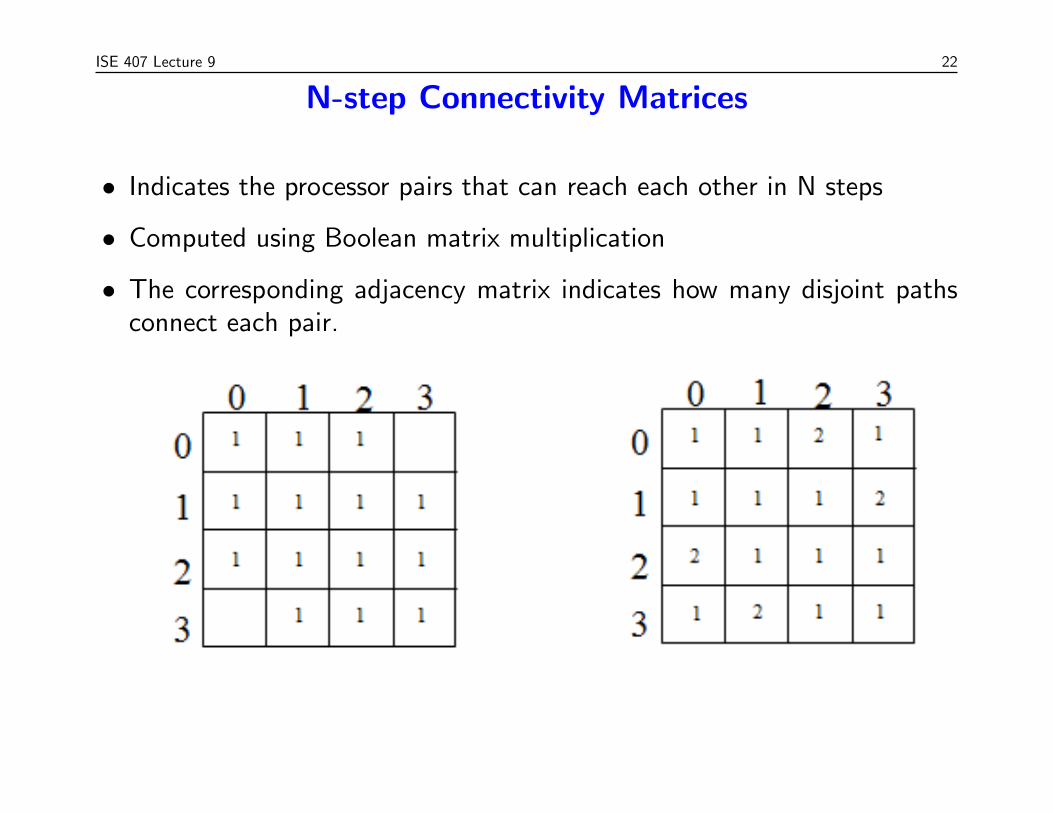
• Indicates the processor pairs that can reach each other in N steps

• Computed using Boolean matrix multiplication

• The corresponding adjacency matrix indicates how many disjoint pathsconnect each pair.

22


Linear Array

23


Ring

24


Mesh

25


Tree

26


Other Schemes

• Pyramid: A 4-ary tree where each level is connected as a mesh

• Hypercube: Two processors are connected if and only if their ID #’sdiffer in exactly one bit.

– Low communications diameter– High bisection width– Doesn’t have constant degree

• Perfect Shuffle: Processor i is connected one-way to processor 2imod N − 1.

• Others: Star, De Bruijn, Delta, Omega, Butterfly

27


Asymptotic Analysis of Parallel Algorithm

• In the course of a parallel architecture, small details make a difference.

• Example: broadcasting a unit of data

– Θ(1) under the shared-memory CREW model– Θ(n) under the shared-memory EREW model– Θ(

√n) under the distributed-memory CREW model on a mesh

– Θ(log n) under the distributed-memory tree model

• Note: These models are architecture dependent

• This is the biggest difference between sequential and parallel complexityanalysis

28


Cost of a Parallel Algorithm

• In the case of a RAM algorithm, the measure of effectiveness was thetime (number of steps).

• In the PRAM case, we may consider both time and “cost.”

– Running time is the number of steps required in “real time.”– Parallel cost is the product of running time and number of cores.

• An “optimal” parallel algorithm is one for which the parallel cost functionis of the same order as the sequential running time function.

• The difference between the sequential running time and the parallel costis known as parallel overhead.

• It consists of time steps during which a core is idle or doing somethingnot required in the parallel algorithm (e.g., moving data).

• For algorithms that are not optimal, the running time decreases withadditional cores, but the cost increases.

29


Speedup and Parallel Efficiency

• Speedup and parallel efficiency are concepts related to parallel cost.

• Speedup is the ratio of the parallel running time to the sequential runningtime.

• Efficiency is the speedup divided by the number of cores.

• Optimal algorithms are those whose speedup is equal to the number ofcores or with a parallel efficiency of 1.

• Essentially, these are algorithms that balance communication and idletime with time for computation.

30


Semigroup operations

• Definition: A binary associative operation

(x⊗ y)⊗ z = x⊗ (y ⊗ z)

• Typical semigroup operations.

– maximum– minimum– sum– product– OR

• Can be used to compare parallel architectures.

31


Semigroup operations example

• RAM Algorithm: Can’t do better than sequential search, which is Θ(n).

• Shared-memory PRAM AlgorithmAssumptions: n cores, CREWInput: An array x = [x1, x2, ..., x2n] (2 data elements per core initially)Output: The smallest entry of X

1 for (i = 0; i < log2(n); i++){

2 parallel for (j = 0; j < 2**(log2(n)-i-1); j++){

3 read x[2j-1] and x[2j];

4 write min(x2j-1, x2j);

5 }

6 }

32


Semigroup operations example (cont’d)

• The parallel cost of this implementation is Θ(n lg n), so this is not costoptimal.

• Can we achieve cost optimality?

– Starting with one data element per core, we can’t expect a runningtime better than Θ(lg n).

– The problem is that we are not fully utilizing all the cores.– Including the idle time, there is an overall increase of the number of

total steps required of lg n.– How do we improve this situation?

33


Scaling Up

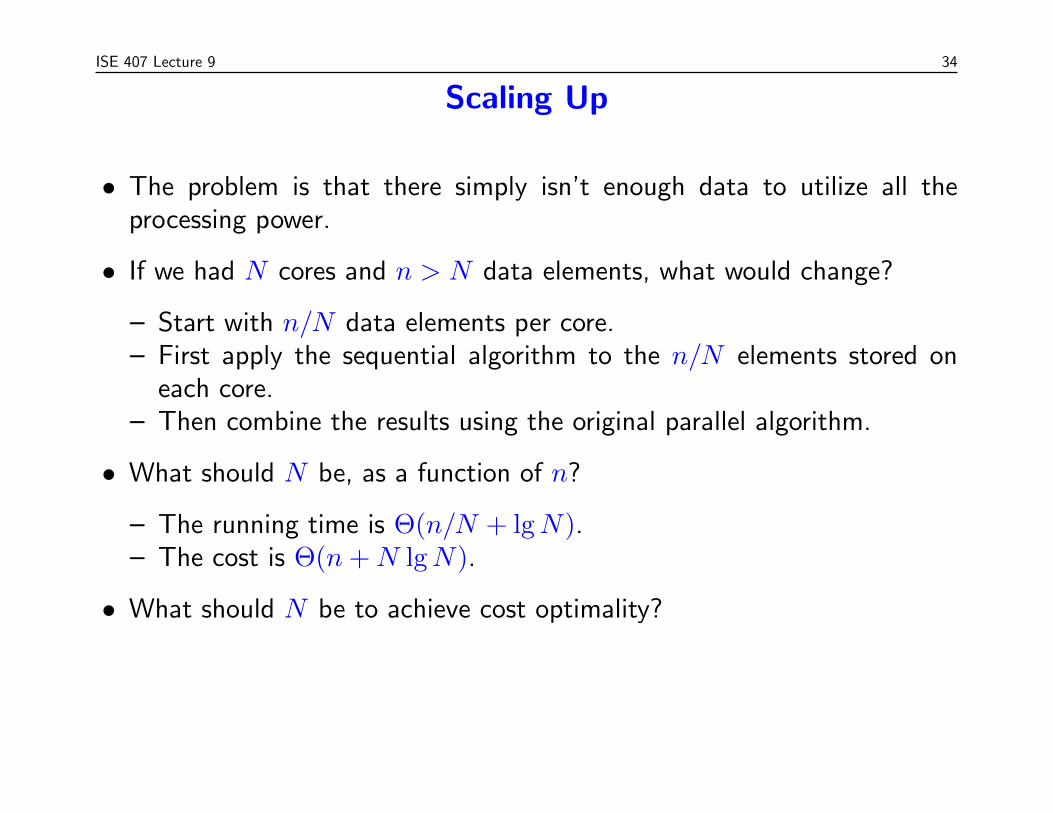
• The problem is that there simply isn’t enough data to utilize all theprocessing power.

• If we had N cores and n > N data elements, what would change?

– Start with n/N data elements per core.– First apply the sequential algorithm to the n/N elements stored on

each core.– Then combine the results using the original parallel algorithm.

• What should N be, as a function of n?

– The running time is Θ(n/N + lgN).– The cost is Θ(n + N lgN).

• What should N be to achieve cost optimality?

34


Scaling Up

• The problem is that there simply isn’t enough data to utilize all theprocessing power.

• If we had N cores and n > N data elements, what would change?

– Start with n/N data elements per core.– First apply the sequential algorithm to the n/N elements stored on

each core.– Then combine the results using the original parallel algorithm.

• What should N be, as a function of n?

– The running time is Θ(n/N + lgN).– The cost is Θ(n + N lgN).

• What should N be to achieve cost optimality?

– We want N lgN ≈ n.– Taking N = n/ lg n is an approximate solution.

34


The General Principle

• The previous analysis illustrates a general principle.

• When adding more cores, there is a limit based on the size of the inputbeyond which we cannot effectively utilize the additional cores.

• We must scale up the input size along with the number of cores in orderto achieve “scalability.”

• We will examine this phenomena in more detail in a future lecture.

35


Other Benchmark Problems

• Broadcast:

– Send value from one processor to all others– Limited by diameter

• Sorting:

– Sort a list of values– Limited by bisection bandwidth

• Semigroup

– Combine values using a binary associative operator– Requires bandwidth and diameter to be balanced

36

computational optimization ise 407 lecture 9

Documents