computational modelling of fluid load support in articular
TRANSCRIPT

Computational Modelling of Fluid Load Supportin Articular Cartilage
Shuqiang An
Submitted in accordance with the requirements for the degree of
Doctor of Philosophy
The University of Leeds
School of Mechanical Engineering
September 2013

- ii -
The candidate confirms that the work submitted is his own, except where
work which has formed part of jointly-authored publications has been
included. The contribution of the candidate and the other authors to this
work has been explicitly indicated below. The candidate confirms that
appropriate credit has been given within the thesis where reference has
been made to the work of others.
This copy has been supplied on the understanding that it is copyright
material and that no quotation from the thesis may be published without
proper acknowledgement.
The right of Shuqiang An to be identified as Author of this work has been
asserted by him in accordance with the Copyright, Designs and Patents Act
1988.
© 2013 The University of Leeds and Shuqiang An
- iii -
Jointly Authored Publications
1) An, Shuqiang; Jones Alison; Damion Robin; Fisher John and Jin
Zhongmin. Realistic Fibril Distribution Basing on DT-MRI Data Enhances
Pressurization of Interstitial Fluid in 2D Fibril-Reinforced Cartilage Model.
Podium presentation. Paper No. 0396, Session 66. Annual Meeting of the
Orthopaedic Research Society, 2013, San Antonio, Texas.
This was based on Chapter 2, Chapter 3 and Chapter 4, and was carried out
by the author of this thesis in its entirety.

- iv -
Acknowledgements
First and foremost, I would like to thank my supervisors, Professor John
Fisher, Professor Zhongmin Jin and Dr. Alison Jones. Professor Fisher, my
primary supervisor in the latest two years, has been overviewed my
research project and provided me the most constructive and valuable
advices during my research study. Prof. Jin was my primary supervisor in
the first two years of study and much more than that, a great mentor and a
warm-hearted friend. Jin contributed excellent ideas to this work, from the
determination of the research subjects to the development of the models,
from the presentation of the results to the final correction of this thesis. I am
also very grateful to Dr. Jones for the detailed techniques and valuable
discussion.
This study would not have been possible without the support of Dr.
Robin Damion, school of Physics, who provided the experimental data
implemented to the models in this thesis. I would also like to thank Graham,
Ted and Margret for their computational support.
It is a great pleasure to work in iMBE, where people help each other. In
this group, I received great help from the senior colleagues, Dr. Feng Liu,
Dr. Qingen Meng, Dr. Mohd Juzaila Abd Latif, Dr. Sainath and Dr. Adam in
whatever way possible, especially when I began my PhD.
Finally, I would like to address my thanks to my family. My wife, Jing,
companies and takes care of me all the way throughout the life and study in

- v -
the UK. Also, great appreciation would like to be given to my daughter, Ran,
who shared all of her joys and tears with me in these years.
This work was funded by the Engineering and Physical Sciences
Research Council.

- vi -
List of Abbreviations
BW – Body Weight
CAX4P – Four-node bilinear displacement and pore pressure
C3D20 – Twenty-node linear brick
C3D20RP – Twenty-node quadratic brick and pore pressure, reduced
integration
DT-MRI – Diffusion Tensor Magnetic Resonance Imaging
FE – Finite Element

- vii -
Abstract
Natural articular cartilage is known to be an excellent bearing material
with very low friction coefficient and wear rate. Theoretical and experimental
studies have demonstrated that the interstitial fluid of cartilage is pressurized
considerably under loading to support the applied load, leading to the low
friction coefficient. In this process, collagen fibrils play a vital role to resist
the lateral expansion of cartilage and enhance the pressurization. The
proportion of the total load supported by fluid pressurization in cartilage,
called the fluid load support, is therefore an important parameter in
biotribology and determined as the main aspect of this thesis.
Fibril-reinforced cartilage models were set up to account for the high
pressurization of interstitial fluid. However, the orientation of collagen fibrils
were idealized or simplified; and the models implementing realistic fibril
orientation derived from DT-MRI data did not include viscous effects in both
the solid matrix and the fibril.
This study overcome the limitation of previous models and the major
finding were:
• The peak value of fluid load support in both 2D and 3D fibril-
reinforced models implementing DT-MRI data was increased to greater than
90% from around 60% in the isotropic poroelastic model, due to the
reinforcement by collagen fibril.

- viii -
• The implementation of the realistic fibril orientation in the 3D fibril-
reinforced model increased the value of peak pore pressure (by 15%)
compared to the uniformly reinforced model while the peak contact pressure
was 4.3% lower, making the peak value of fluid load support increase from
80.4% to 96.7%.
• The rationality to define the principal eigenvector as orientation of the
corresponding primary collagen fibril in the fibril-reinforced models was
verified by the related results.
• The feasibility and reliability of the methodologies to implement DT-
MRI data to the fibril-reinforced models were both confirmed in the
modelling process.

- ix -
Table of Contents
Acknowledgements.................................................................................... iv
List of Abbreviations.................................................................................. vi
Abstract...................................................................................................... vii
Table of Contents....................................................................................... ix
List of Tables ............................................................................................ xiv
List of Figures ........................................................................................... xv
Preface ..................................................................................................... xxii
Chapter 1 Introduction and Literature Review........................................ 1
1.1 Introduction .................................................................................. 1
1.2 Synovial Joints and Biomechanics ............................................... 2
1.2.1 Hip joint and knee joint ....................................................... 2
1.2.2 Motion and load.............................................................. 4
1.2.2.1 Motion of hip joint and knee joint............................. 4
1.2.2.2 Joint loading in hip joint and knee joint............. 6
1.3 Articular Cartilage....................................................................... 8
1.3.1 Composition and structure of articular cartilage ................. 8
1.3.1.1 Structure of articular cartilage ................................. 9
1.3.1.2 Composition of articular cartilage ....................... 11
1.3.2 Biphasic lubrication of articular cartilage .......................... 16
1.3.2.1 Interstitial fluid pressurisation .............................. 17
1.3.2.2 Cartilage lubrication by interstitial fluid loadsupport ........................................................................ 21
1.4 Computational Modelling of Articular Cartilage .......................... 24
1.4.1 The biphasic background ................................................. 27
1.4.2 The macrostructural FE models of articular cartilage ....... 28
1.4.2.1 The isotropic poroelastic model............................. 28
1.4.2.2 The transversely isotropic poroelastic model ........ 28
1.4.3 The microstructural FE models of articular cartilage ........ 31
1.4.3.1 The fibril-reinforced poroelastic model .................. 31
1.4.3.2 Comparison of various fibril-reinforced models ..... 33
1.4.3.3 Comparison of element types used in fibril-reinforced FE models .................................................. 43
1.4.3.4 Methods to define collagen fibril orientation .......... 44
- x -
1.5 Diffusion Tensor Magnetic Resonance Imaging of ArticularCartilage...................................................................................... 49
1.5.1 Diffusion tensor magnetic resonance imaging (DT-MRI) .................................................................................... 50
1.5.2 The primary collagen orientation of articular cartilage...... 50
1.6 Summary of the literature review................................................ 53
1.7 Project Aims and Objectives ................................................... 53
Chapter 2 Analysis of Diffusion Tensor Magnetic Imaging Data ........ 55
2.1 Introduction ................................................................................ 55
2.2 Method to Analyze the DT-MRI Data.......................................... 56
2.2.1 Material ............................................................................ 56
2.2.2 The Diffusion Tensor MRI scanning and pixeldefinitions............................................................................ 57
2.2.3 Method for analysing the principal eigenvectors .............. 58
2.2.3.1 The 2D quiver plots ................................................. 58
2.2.3.2 Analysis of the angles between the principaleigenvectors and the cartilage surface........................ 59
2.3 Results ....................................................................................... 60
2.3.1 Two-dimensional quiver plots........................................... 60
2.3.2 Distribution of fibril angles to cartilage surface ................. 62
2.3.2.1 Fibril angles in the top two layers ............................ 62
2.3.2.2 Fibril angles in layers from the 3rd to 9th ................ 63
2.3.2.3 Fibril angles in layers from the 10th to 17th............. 68
2.4 Discussion.................................................................................. 71
Chapter 3 Material Model and Method to ImplementDT-MRI Data....................................................................................... 74
3.1 Introduction ................................................................................ 74
3.2 Material Model............................................................................ 75
3.2.1 The Jacobian matrix of fibril-reinforced FE model ............ 76
3.2.2 The contribution of the fibrillar matrix to the Jacobian ..... 77
3.2.3 Simplification for the instantaneous fibrillar modulus........ 78
3.2.4 Implementation in commercial FE software...................... 79
3.3 Methods to Implement DT-MRI Data in the 2D Model................ 80
3.3.1 Geometry and mesh of the 2D model............................... 80
3.3.2 Definition of the element level Cartesian coordinatesin the 2D model ................................................................... 81
3.4 Method to Implement DT-MRI Data in the 3D model.................. 84

- xi -
3.4.1 Definition of the element level Cartesian coordinatesin the 3D model ................................................................... 84
3.4.2 Definition of the element level Cartesian coordinatesin the 3D model ................................................................... 86
3.5 Summary.................................................................................... 86
Chapter 4 Effect of Modelling Fibril Orientation in Two-dimensional Axisymmetric Models.................................................. 88
4.1 Introduction ................................................................................ 88
4.2 Model and Method...................................................................... 89
4.2.1 Boundary conditions and load .......................................... 90
4.2.2 Element type and mesh.................................................... 91
4.2.3 Material model.................................................................. 92
4.2.4 Mesh sensitivity analysis of the 2D isotropic model ......... 93
4.2.5 Parameter predictions of 2D models ................................ 96
4.3 Modelling Cases......................................................................... 98
4.3.1 Models of the DT-MRI based group ............................... 100
4.3.1.1 Mechanical property of material ............................ 100
4.3.1.2 Implementation of fibril orientation ........................ 101
4.3.2 Models of the uniform reinforced group.......................... 103
4.3.2.1 Mechanical property of material ............................ 103
4.3.2.2 Definition of the local coordinate system............... 105
4.3.3 The isotropic poroelastic model...................................... 105
4.4 Results ..................................................................................... 106
4.4.1 Contact pressure, pore pressure and fluid loadsupport on cartilage surface.............................................. 107
4.4.2 The fluid velocity of cartilage .......................................... 111
4.4.3 The contour of pore pressure within cartilage ................ 113
4.4.4 The radial and axial deformation of the cartilage openedge .................................................................................. 115
4.4.4.1 The radial deformation of nodes on the openedge of cartilage........................................................ 115
4.4.4.2 The axial deformation of the cartilage open edge . 116
4.4.5 The radial stress on the cartilage surface....................... 118
4.4.6 The axial deformation of cartilage during loadingperiod ................................................................................ 118
4.5 Discussion................................................................................ 119
4.5.1 The effect of the user defined subroutine “UMAT” ......... 120
4.5.1.1 The effect on the surface zone of cartilage ........... 120

- xii -
4.5.1.2 The effect on pore pressure and fluid velocitythroughout the cartilage ............................................ 121
4.5.2 The influence of the realistic fibril orientation ................. 122
4.5.3 The effect of strain dependent Young’s modulus ........... 123
4.5.4 Limitation of the 2D axisymmetric DT-MRI model .......... 123
Chapter 5 Three-dimensional Fibril-reinforced Model ....................... 125
5.1 Introduction .............................................................................. 125
5.2 Model and Method.................................................................... 126
5.2.1 Geometry of the 3D models ........................................... 126
5.2.2 Boundary conditions and load ........................................ 127
5.2.3 Material model................................................................ 128
5.2.4 Mesh of the 3D models .................................................. 128
5.2.4.1 Element type ........................................................ 128
5.2.4.2 Mesh of the 3D model .......................................... 129
5.2.5 Mesh sensitivity analysis of the 3D isotropic model ....... 130
5.2.6 Method to implement the DT-MRI data .......................... 132
5.2.7 Outputs from the 3D models .......................................... 133
5.2.7.1 Contact pressure, pore pressure, fluid loadsupport and stress on the surface of cartilage .......... 134
5.2.7.2 The fluid velocity and contour of pore pressure.... 135
5.2.7.3 Deformation of the cartilage ................................. 136
5.3 Modelling Cases....................................................................... 137
5.3.1 The 3D fibril reinforced model ........................................ 138
5.3.1.1 Mechanical property of material ........................... 138
5.3.1.2 Implementation of fibril orientation ....................... 140
5.3.2 The 3D uniformly reinforced model ................................ 141
5.3.2.1 Mechanical property of material ........................... 141
5.3.2.2 Definition of the local coordinate system.............. 142
5.3.3 The isotropic poroelastic model...................................... 143
5.4 Validation of the 3D DT-MRI based model ............................... 144
5.5 Results ..................................................................................... 146
5.5.1 Comparison of results from different 3D models ............ 146
5.5.1.1 Contact pressure, pore pressure and fluid loadsupport on the cartilage surface................................ 146
5.5.1.2 Distribution of fluid velocity................................... 157
5.5.1.3 Deformation of the cartilage ................................. 161

- xiii -
5.5.1.4 Stress on the cartilage surface............................. 167
5.5.2 Validation results of the 3D DT-MRI based model.......... 171
5.6 Discussion................................................................................ 173
5.6.1 The effect of fibril reinforcement..................................... 174
5.6.1.1 The effect on pore pressure and fluid loadsupport on the cartilage surface................................ 174
5.6.1.2 The effect on pore pressure and fluid velocityinside the whole cartilage.......................................... 175
5.6.2 The influence of the realistic fibril orientation ................. 177
5.6.2.1 The influence on the stress along the global X-axis (S11).................................................................. 178
5.6.2.2 The influence on the distribution of contactpressure on cartilage surface.................................... 178
5.6.3 Limitation of the DT-MRI-3D model................................ 179
Chapter 6 Overall Discussion and Conclusions.................................. 181
6.1 Fibril Reinforced Finite Element Modelling of ArticularCartilage.................................................................................... 181
6.1.1 Material models of cartilage ........................................... 182
6.1.2 Realistic orientation of collagen fibril .............................. 183
6.1.3 The 2D axisymmetric fibril-reinforced model .................. 184
6.1.4 The 3D fibril-reinforced model ........................................ 185
6.1.5 Limitations ...................................................................... 187
6.2 The Conclusions....................................................................... 189
6.3 Further Work ............................................................................ 190
List of References ................................................................................... 192
Appendix A List of Publications ............................................................ 207
Appendix B Derivation of the Contribution of Fibillar Matrix .............. 208

- xiv -
List of Tables
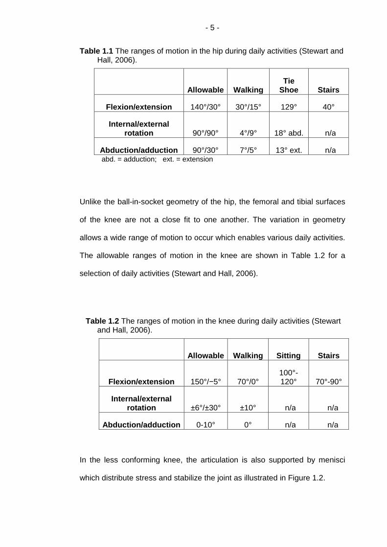
Table 1.1 The ranges of motion in the hip during daily activities(Stewart and Hall, 2006). ..................................................................... 5
Table 1.2 The ranges of motion in the knee during daily activities(Stewart and Hall, 2006). ..................................................................... 5
Table 1.3 Joint loading in the hip and knee (Stewart and Hall,2006). .................................................................................................... 7
Table 1.4 Transversely isotropic biphasic properties of bovinedistal ulnar growth plate and chondroepiphysis obtainedfrom confined and unconfined compression tests (means ±std. dev.): (a) elastic moduli; (b) permeability coefficients(Cohen et al. 1998) ............................................................................ 30
Table 1.5 Fibril-reinforced FE models of articular cartilage. ............... 34
Table 1.6 Comparison of different element types to implementcollagen fibril direction in fibril-reinforced FE models: ................. 44
Table 4.1 Material parameters of isotropic model. ................................. 93
Table 4.2 Material properties of different models (ε is the fibrillarstrain in each iteration and initial void ratio 4.0 represented80% interstitial fluid). ........................................................................ 99
Table 4.4 Comparison of results on axisymmetric surface centreof cartilage sample at the end of ramp loading (t = 2s). .............. 110
Table 5.1 Material properties of different models (ε is the fibrillarstrain in each iteration and 4.0 represented 80% interstitialfluid). ................................................................................................ 138

- xv -
List of Figures
Figure 1.1 Hip Joint (Orthopaedics,2007).................................................. 3
Figure 1.2 Knee joint (Tandeter et al., 1999). ............................................ 4
Figure 1.3 Schematic depiction of cartilage composition (source:www.bidmc.org/ Research/Departments/Radiology/Laboratories/ Cartilage). ..................................................................... 8
Figure 1.4 Schematic depiction of articular cartilage’s structure(Buckwalter et al., 1994)...................................................................... 9
Figure 1.5 Schematic depiction of PG structure (Larry W, 2003) .......... 12
Figure 1.6 (a) Cartilage surface showing the creation of the splitlines with a dissecting needle that has been dipped in Indiaink; (b) Photograph showing the split-line pattern of a distalfemoral specimen (Steven et al., 2002)............................................ 13
Figure 1.7 Bovine cartilage: (a) Collagen columns runperpendicular to the surface. (b) A column consists ofparallel collagen, perpendicular to the surface in the deepzone (Kaab et al., 1998)..................................................................... 14
Figure 1.8 Light micrographs of normal adult human articularcartilage originating from (a) the superficial zone, (b) themiddle zone, and (c) the lower deep zone (Thomas et al.,2005). .................................................................................................. 16
Figure 1.9 The stress-relaxation response shows a characteristicstress increase during the compressive phase and then thestress decreases during the relaxation phase untilequilibrium is reached (point e). Fluid flow and solid matrixdeformation during the compressive process give rise to thestress-relaxation phenomena (Mow et al., 1989). ........................... 19
Figure 1.10 Confined compression creep response of bovinearticular cartilage (square symbols denote experimental dataand the solid curve represents a curve-fit of the experimentalresponse using the biphasic theory): (a) creep deformationversus time; (b) Ratio of interstitial fluid pressure to appliedstress, at the cartilage face abutting the bottom of theconfining chamber (Soltz et al., 1998). ............................................ 20
Figure 1.11 (a)Time-dependent response of the friction coefficientμeff and interstitial fluid load support Wp/W (b) A linearvariation plot of μeff versus Wp/W (Krishnan et al., 2004)............... 23
Figure1.12 Diagram of the model showing the isotropic matrix(containing pores) and the fibrils evenly distributed in thethree orthogonal directions (Li et al., 1999). ................................... 35

- xvi -
Figure 1.13 Mesh for the finite elements illustrating also thearrangement of spring elements in a porous continuumelement. Displacements are interpolated by all nodes, but thepore pressure is interpolated by four corner nodes only (Li etal., 1999). ............................................................................................ 37
Figure 1.14 A typical shell membrane element with materialprincipal axes that are oriented along the principal straindirections in the plane of the membrane at any givenintegration point I. The tangent modulus matrix in thissystem is also shown neglecting the cross coupling termsbetween incremental normal stresses and strains (i.e., ν = 0).(Shirazi et al., 2005). .......................................................................... 41
Figure 1.15 Finite element mesh of the model showing thearrangement of horizontal and vertical membrane elements ina typical axisymmetric porous continuum element (Shirazi etal., 2005). ............................................................................................ 42
Figure 1.16 The porous, nonfibrillar matrix of cartilage isrepresented with 2D pore pressure elements and therandomly distributed collagen fibrils are modeled with 1Dembedded rebar elements oriented in 15 different directionsat 0˚, ±30˚ and ±60˚ from the r, z and θ axes (Gupta et al., 2009). .................................................................................................. 45
Figure 1.17 Orientation of the primary fibrils as a function ofdepth. Right: cartoon of the arcade model of Benninghoff(1925). Left: Orientation of four primary collagen fibrils asimplemented in the model (Wilson et al., 2004).............................. 47
Figure 1.18 Schematic representation of the 13 differentorientations of the secondary fibrils at any arbitrary point inthe fibrillar matrix (Wilson et al., 2004)............................................ 48
Figure 1.19 Primary collagen orientations of a piece of articularcartilage located on a distal femur. Four different fiberorientations were considered as shown with A, B, C and Dzones. The size of the tissue considered is 14 × 10 × 2 mmwith 2 mm in the depth (Li et al., 2009)............................................ 49
Figure 1.20 2D quiver plots of the collagen fibril, (a) beforecompression and after two subsequent compressions (b) by18% and (c) by 29% of the original cartilage thickness,respectively (Meder et al. 2006). ...................................................... 51
Figure 2.1 Schematic diagram of cartilage specimen scannedusing MRI. The Y-axis was defined as into pageperpendicular to the X and Z axes (Modified from Pierce etal., 2010). ............................................................................................ 57
Figure 2.2 X-Z components of principal eigenvector of diffusiontensor. (Z axis shows the row number, and X axis shows thecolumn number of the pixel grid; provided by Dr RobinDamion).............................................................................................. 61

- xvii -
Figure 2.3 Bar chart of fibril angle of pixels in the top 2 layers ofcartilage. ............................................................................................ 62
Figure 2.4 Fibril angle distribution of pixels in top 2 layers fromcartilage surface................................................................................ 63
Figure 2.5 Bar chart of fibril angle of pixels in the 3rd and 4th layerof cartilage. ........................................................................................ 64
Figure 2.6 Fibril angle distribution of pixels in the 3rd and 4th layerfrom cartilage surface....................................................................... 65
Figure 2.7 Bar chart of fibril angle of pixels in the 5th - 9th layerfrom cartilage surface....................................................................... 66
Figure 2.8 Fibril angle distribution of pixels in the 5th - 9th layerfrom cartilage surface....................................................................... 67
Figure 2.9 Fibril angle distribution of elements in 10th - 15th layerfrom cartilage surface....................................................................... 68
Figure 2.10 Bar chart of fibril angle of pixels in the 10th - 15th layerfrom cartilage surface....................................................................... 69
Figure 2.11 Bar chart of fibril angle of pixels in the 16th and 17th
layer from cartilage surface. ............................................................ 70
Figure 2.13 Fibril angle distribution of elements in 16th and 17th
layer from cartilage surface. ............................................................ 71
Figure 3.1 2D mesh corresponds to the pixel grid: (vertical axis:Z(2); horizontal axis: X (1)). .............................................................. 80
Figure 3.2 3-points method to define the local rectangular system(Abaqus Analysis user’s manual Figure 2.2.5-1)........................... 81
Figure 3.3 “Distribution” to define the local rectangular system foreach element in 2D models (Abaqus Analysis user’s manual2.7.1). .................................................................................................. 83
Figure 3.4 Flow chart of to implement DT-MRI data and “UMAT” inthe 2D fibril-reinforced model. ......................................................... 84
Figure 3.5 Definition of local Y-axis (vector )................................... 85
Figure 3.6 ‘Distribution’ to define the local rectangular system foreach element in 3D models (Abaqus Analysis user’s manual2.7.1). .................................................................................................. 86
Figure 4.1 Schematic diagram of articular cartilage underunconfined compression.................................................................. 90
Figure 4.2 Schematic diagram of the 2D axisymmetric FE modelsimulating articular cartilage under unconfined compression(vertical axis: Z; horizontal axis: X (r); into plane axis: Y (θ)). ...... 92
Figure 4.3 Distribution of contact pressure on cartilage surface atthe end of ramp load (t = 2s). ........................................................... 94
Figure 4.4 Distribution of pore pressure on cartilage surface at theend of ramp load (t = 2s)................................................................... 95

- xviii -
Figure 4.5 Fluid load support at cartilage surface node on thesymmetry axis of different mesh density at the end of rampload (t = 2s). ....................................................................................... 96
Figure 4.6 Adjustments of Young’s modulus in the Cons E modelto achieve the same maximum axial displacement as DT-MRImodel at the end of ramp loading (t = 2s). .................................... 104
Figure 4.7 Adjustments of Young’s modulus in the ISO model toachieve the same maximum axial displacement as DT- MRImodel at the end of ramp loading (t = 2s). .................................... 106
Figure 4.8 Distribution of contact pressure along cartilage surfaceat the end of ramp loading (t = 2s)................................................. 107
Figure 4.9 Distribution of pore pressure along cartilage surface atthe end of ramp loading (t = 2s). .................................................... 108
Figure 4.10 Comparison of fluid load support along cartilagesurface at the end of ramp loading (t = 2s). .................................. 109
Figure 4.11 Comparison of fluid load support at the centre ofcartilage surface during loading period. ....................................... 111
Figure 4.12 Fluid velocity (mm/s) of (a) Isotropic, (b) Uniform-Cons, (c) Uniform-SD, (d) DT-MRI and (e) DT-MRI-top at theend of ramp loading (t = 2s). .......................................................... 112
Figure 4.13 Contour of pore pressure (MPa) of (a) Isotropic, (b)Uniform-Cons, (c) Uniform-SD, (d) DT-MRI and (e) DT-MRI-topmodel at the end of ramp loading (t = 2s). .................................... 114
Figure 4.14 Comparison of radial deformation on open edge ofcartilage at the end of ramp loading (t = 2s). ................................ 115
Figure 4.15 Comparison of axial displacement of nodes along theopen edge of cartilage at the end of ramp loading (t = 2s). ......... 116
Figure 4.16 Comparison of axial deformation of elements alongthe open edge of cartilage at the end of ramp loading (t = 2s).... 117
Figure 4.17 Distribution of radial stress (S11) along cartilagesurface at the end of ramp loading (t = 2s). .................................. 118
Figure 4.18 Normalized axial deformation of cartilage during theloading period (3602s). ................................................................... 119
Figure 5.1 The structured pixel grid of diffusion tensor MRI (17rows and 74 columns)..................................................................... 127
Figure 5.2 Mesh of the 3D fibril-reinforced cartilage model with8×17×74 elements. .......................................................................... 129
Figure 5.3 Comparison of contact pressure (a), pore pressure (b)and fluid load support (c) at the centre of cartilage surface inisotropic models with different number of elements duringthe simulation (t=3600s). ................................................................ 131

- xix -
Figure 5.4 Comparison of axial displacement of cartilage surfacein isotropic models with different number of elements duringthe simulation (t=3600s). ................................................................ 132
Figure 5.5 Paths defined on the cartilage surface to collect thedata of related measurements in the 3D models (a) Midline-Yparallel to the global Y-axis; (b) Midline-X parallel to theglobal X-axis (from right to left). .................................................... 134
Figure 5.6 The two cross-sections to investigate the distributionsof related measurements inside cartilage in the 3D models:(a) the cross-section perpendicular to the global X-axis; (b)the cross-section perpendicular to the global Y-axis. ................. 136
Figure 5.7 Fluid load support along the Midline-X on cartilagesurface parallel to the global X-axis in the DT-MRI-3D modelswith different values of Young’s modulus Em of thenonfibrillar at the end of ramp loading (t = 2s). ........................... 139
Figure 5.8 Adjustments of Young’s modulus in the Uniform-3Dmodel to achieve the same axial displacement of cartilagesurface centre as DT-MRI-3D model at the end of ramploading (t = 2s)................................................................................. 142
Figure 5.9 Adjustments of Young’s modulus in the Isotropic-3Dmodel to achieve the same axial displacement of cartilagesurface centre as the DT-MRI-3D model at the end of ramploading (t = 2s)................................................................................. 143
Figure 5.10 Normalized vertical displacements (%) of cartilagesurface in the creep test. ................................................................ 145
Figure 5.11 Comparison of contact pressure on the cartilagesurface along (a) Midline-X and (b) Midline-Y at the end oframp loading (t = 2s). ...................................................................... 147
Figure 5.12 Comparison of pore pressure on the cartilage surfacealong (a) Midline-X and (b) Midline-Y at the end of ramploading (t = 2s)................................................................................. 148
Figure 5.13 Comparison of fluid load support on the cartilagesurface along (a) Midline-X and (b) Midline-Y at the end oframp loading (t = 2s). ...................................................................... 149
Figure 5.14 Contour of contact pressure (MPa) on the cartilagesurface of (a) the Isotropic-3D, (b) the Uniform-3D and (c) theDT-MRI-3D model at the end of ramp loading (t = 2s). ................. 150
Figure 5.15 Contour of pore pressure (MPa) on the cartilagesurface of (a) the Isotropic-3D, (b) the Uniform-3D and (c) theDT-MRI-3D at the end of ramp loading (t = 2s).............................. 151
Figure 5.16 Contour of pore pressure (MPa) on the cross-sectionperpendicular to the global X-axis (out of the page) of (a) theIsotropic-3D, (b) the Uniform-3D and (c) the DT-MRI-3D modelat the end of ramp loading (t = 2s)................................................ 153

- xx -
Figure 5.17 Contour of pore pressure (MPa) on the cross-sectionperpendicular to the global Y-axis (out of the page) of (a) theIsotropic-3D, (b) the Uniform-3D and (c) the DT-MRI-3D modelat the end of ramp loading (t = 2s)................................................. 154
Figure 5.18 Comparison of fluid load support at cartilage surfacecentre during the loading period (t = 3602s)................................. 156
Figure 5.19 Distribution of fluid velocity (mm/s) on the verticalouter sides of cartilage in (a) the Isotropic-3D, (b) theUniform-3D and (c) the DT-MRI-3D model at the end of ramploading (t = 2s)................................................................................. 157
Figure 5.20 Distribution of fluid velocity (mm/s) on the cross-section perpendicular to the global X-axis (out of the page) of(a) the Isotropic-3D, (b) the Uniform-3D and (c) the DT-MRI-3Dmodel at the end of ramp loading (t = 2s). .................................... 159
Figure 5.21 Distribution of fluid velocity (mm/s) on the cross-section perpendicular to the global Y-axis (out of the page) of(a) the Isotropic-3D, (b) the Uniform-3D and (c) the DT-MRI-3D model at the end of ramp loading (t = 2s)................................ 160
Figure 5.22 Comparison of radial deformation of cartilage on thedirection of (a) global X-axis and (b) global Y-axis at the endof ramp loading (t = 2s)................................................................... 161
Figure 5.23 Comparison of vertical deformation of cartilage layersalong (a) Midline-Y-Z and (b) Midline-X-Z at the end of ramploading (t = 2s)................................................................................. 163
Figure 5.24 Comparison of vertical deformation of elements alongMidline-X and the two cartilage surface edge in global X-Zplane at the end of ramp loading (t = 2s). ..................................... 164
Figure 5.25 Comparison of vertical deformation of cartilage layersin global Y-Z plane at the end of ramp loading (t = 2s). ............... 166
Figure 5.26 Comparison of vertical displacement of cartilagesurface centre during loading period. ........................................... 167
Figure 5.27 Comparison of stress: (a) S11 (kPa) along Midline-Xand (b) S22 (kPa) along Midline-Y at the end of ramp loading (t= 2s).................................................................................................. 168
Figure 5.28 Stress along global X-axis (S11; MPa) on cartilagesurface of (a) the Isotropic-3D, (b) the Uniform-3D and (c) theDT-MRI-3D model at the end of ramp loading (t = 2s). ................. 169
Figure 5.29 Stress along global Y-axis (S22; MPa) on cartilagesurface of (a) the Isotropic-3D, (b) the Uniform-3D and (c) theDT-MRI-3D model at the end of ramp loading (t = 2s). ................. 170
Figure 5.30 Comparison of axial deformation of cartilage inexperiment and modelling with different Young’s modulus ofthe nonfibrillar matrix (t = 2250s)................................................... 172

- xxi -
Figure 5.31 Comparison of axial deformation of cartilage inexperiment and modelling with different Young’s modulusand permeability of the nonfibrillar matrix (t = 2250s). ................ 173

- xxii -
Preface
In Loving Memory of My Mother

- 1 -
Chapter 1 Introduction and Literature Review
1.1 Introduction
This chapter reviews the literature relevant to the biomechanics and
computational modeling of articular cartilage in the synovial joints. The
material properties of articular cartilage are key factors in determining the
lubrication of the joints. Therefore, the related literature on cartilage
composition and structure including the biphasic lubrication is introduced
first, after a brief review on the biomechanics of the two main synovial joints
- knee and hip. The literature on the computational modelling of cartilage is
reviewed in detail, particularly the fibril reinforced finite element models. As
the collagen fibril orientations used in the models of this thesis were derived
from the Diffusion Tensor Magnetic Resonance Imaging (DT-MRI)
experiments, the related methodologies are also introduced as the
background.
The review begins with a brief introduction to the biomechanics of knee and
hip. The structure of these two largest synovial joints in the human body are
introduced, followed a summary of the motion and loading of the joints.
The second part focuses on the articular cartilage. The detailed composition
and structure of cartilage are reviewed. Then the concepts and viewpoints of
the theory of biphasic lubrication within synovial joints are introduced.
The following section examines the literature relating to the computational
modelling of cartilage. The developments of computational modelling

- 2 -
techniques are discussed. The current methods to set up the fibril reinforced
finite element models are categorized and reviewed individually.
In order to give a better understanding on the background of the thesis, the
final section presents a review on the diffusion tensor MRI.
At the end of this chapter, the rationale and objectives of the project studied
in this thesis are presented.
1.2 Synovial Joints and Biomechanics
The joints of the human body can be classified into three groups: fibrous,
cartilaginous and synovial. Fibrous joints are those in which the bony
surfaces have very little relative motion, a good example being the bones in
the skull. Cartilaginous joints are those in which the bony surfaces have a
little more relative motion such as the joint between two adjacent vertebrae.
The third type are synovial (or diarthrodial) joints, for example the knee joint
and hip joint, which are the joints focused on in this thesis.
1.2.1 Hip joint and knee joint
The hip joint can be considered as a ball-and-socket joint (Figure 1.1). This
arrangement enables the hip to have a large amount of motion needed for
daily activities like walking, squatting, and stair-climbing. The bones of the
hip are the femur and the pelvis. The top end of the femur is shaped like a
ball called the femoral head. The femoral head fits into a spherical socket on
the side of the pelvis. This socket is called the acetabulum. The femoral
head is attached to the rest of the femur (Figure 1.1).
- 3 -
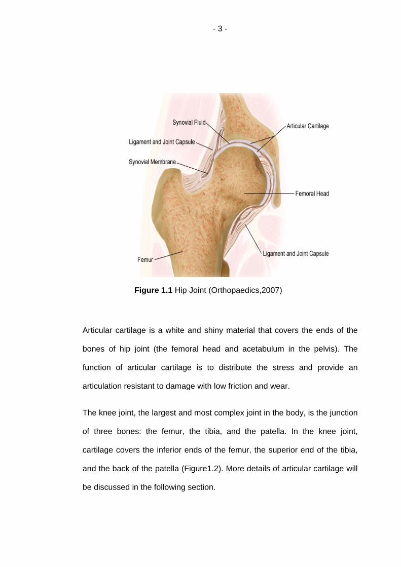
Figure 1.1 Hip Joint (Orthopaedics,2007)
Articular cartilage is a white and shiny material that covers the ends of the
bones of hip joint (the femoral head and acetabulum in the pelvis). The
function of articular cartilage is to distribute the stress and provide an
articulation resistant to damage with low friction and wear.
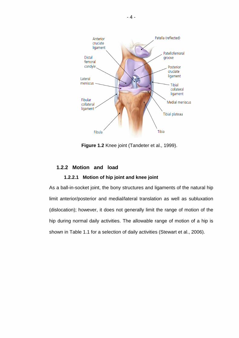
The knee joint, the largest and most complex joint in the body, is the junction
of three bones: the femur, the tibia, and the patella. In the knee joint,
cartilage covers the inferior ends of the femur, the superior end of the tibia,
and the back of the patella (Figure1.2). More details of articular cartilage will
be discussed in the following section.
- 4 -
Figure 1.2 Knee joint (Tandeter et al., 1999).
1.2.2 Motion and load
1.2.2.1 Motion of hip joint and knee joint
As a ball-in-socket joint, the bony structures and ligaments of the natural hip
limit anterior/posterior and medial/lateral translation as well as subluxation
(dislocation); however, it does not generally limit the range of motion of the
hip during normal daily activities. The allowable range of motion of a hip is
shown in Table 1.1 for a selection of daily activities (Stewart et al., 2006).
- 5 -
Table 1.1 The ranges of motion in the hip during daily activities (Stewart andHall, 2006).
Allowable WalkingTie
Shoe Stairs
Flexion/extension 140°/30° 30°/15° 129° 40°
Internal/externalrotation 90°/90° 4°/9° 18° abd. n/a
Abduction/adduction 90°/30° 7°/5° 13° ext. n/aabd. = adduction; ext. = extension
Unlike the ball-in-socket geometry of the hip, the femoral and tibial surfaces
of the knee are not a close fit to one another. The variation in geometry
allows a wide range of motion to occur which enables various daily activities.
The allowable ranges of motion in the knee are shown in Table 1.2 for a
selection of daily activities (Stewart and Hall, 2006).
Table 1.2 The ranges of motion in the knee during daily activities (Stewartand Hall, 2006).
Allowable Walking Sitting Stairs
Flexion/extension 150°/−5° 70°/0°100°-120° 70°-90°
Internal/externalrotation ±6°/±30° ±10° n/a n/a
Abduction/adduction 0-10° 0° n/a n/a
In the less conforming knee, the articulation is also supported by menisci
which distribute stress and stabilize the joint as illustrated in Figure 1.2.
- 6 -
1.2.2.2 Joint loading in hip joint and knee joint
Typical loads measured within the body during various activities for the hip
and knee are shown in Table 1.3. The walking cycle is characterised by two
peaks of load at heel-strike and at toe-off which generally range from 3 to 4
times body weight (BW; Table 1.3; Paul, 1966). Between the two loading
peaks the mass of the body (head and torso) does not exhibit any significant
translation in the vertical direction, so the reaction force during this period is
relatively small.
At toe-off the hip is extended 15° (Table 1.1). The quadriceps muscle acts to
stabilise the knee whilst the gastrocnemius muscle produces plantar flexion
at the ankle. These muscle forces combine to accelerate the body forward
producing the second peak of load in the reaction force curve (Stewart and
Hall, 2006).

- 7 -
Table 1.3 Joint loading in the hip and knee (Stewart and Hall, 2006).
Activity Reference Hip load Knee load
Walking
Freeman andPinskerova 3.4 BW
Paul 3–4 BW 3 BW
Bergmann et al. (in vivonormal) 2–3 BW
Bergmann et al. (in vivodefective) 3–4 BW
Stair
ascent/
descent
Freeman andPinskerova 4.8/4.3 BW
Costigan et al. 3–6 BW
Paul 4.4/4.9 BW
Bergmann et al. (in vivonormal) 2–3.5 BW
Bergmann et al. (in vivodefective)
3.5–5 BW
Risingfrom
a chair
Ellis et al. 3.2 BW
Bergmann et al. (in vivonormal) 1.75–2.25 BW
Risingfrom asquat
Dahlkvist et al. 4.7–5.6 BW
Paul 4.2 BW(BW = Body Weight)

- 8 -
1.3 Articular Cartilage
1.3.1 Composition and structure of articular cartilage
Articular cartilage can be considered as a solid matrix saturated with water
and mobile ions. The solid matrix consists of chondrocytes embedded in
extracellular matrix. The two major components of the extracellular matrix
are collagen fibres composed of collagen fibrils and proteoglycans (PGs)
which are large, complex biomolecules composed of a central protein core
with negatively charged glycoaminoglycan (GAG) side chains looking like
bottle-brushes (Figure 1.3; Maroudas, 1975).
Figure 1.3 Schematic depiction of cartilage composition (source:www.bidmc.org/ Research/Departments/Radiology/ Laboratories/Cartilage).

- 9 -
1.3.1.1 Structure of articular cartilage
Articular cartilage can be divided into four different layers, or zones. Moving
from exposed surface to interface with subchondral bone, these layers are
the superficial or the superficial transitional zone (STZ); the middle zone; the
deep zone and the calcified cartilage zone (Figure 1.4).
Figure 1.4 Schematic depiction of articular cartilage’s structure (Buckwalteret al., 1994)
Superficial zone
The superficial surface zone is the thinnest and forms the gliding surface of
the joint. Collagen and water content are highest in this zone, (water content
is approximately 85%; Maroudas 1979). The chondrocytes appear flattened
and are relatively inactive. Cell volume is smaller, cell density is higher
(Figure 1.4 A) and aggrecan content is lower in the superficial zone
compared to the deeper zones. Collagen fibres are densely packed, have a
small diameter, and are arranged parallel to the articular surface (Figure 1.4

- 10 -
B; Wong et al., 1996). Collagen and PGs appear to be strongly
interconnected in this zone, which may help the superficial zone to resist
shear stresses produced by motion (Mow et al., 2002).
Middle zone
The middle zone occupies several times the volume of the superficial zone.
The collagen fibres are more randomly arranged and have a larger diameter
than in the superficial zone (Figure 1.4 B, Hasler et al., 1999). The
chondrocytes appear rounded and are larger and more active than in the
superficial zone (Figure 1.4 A). PG content is high in this zone and aggrecan
aggregates are larger than in the superficial zone (Buckwalter et al., 1991).
Deep zone
The collagen fibres have their largest diameters and are arranged
perpendicular to the subchondral bone in the deep zone (Figure 1.4 B;
Hunziker et al., 1997). This zone has the lowest water content
(approximately 60%) and a high PG content (Maroudas, 1975). The
chondrocytes tend to be aligned in radial columns (Figure 1.4 A) and the
synthetic activity of the chondrocytes is highest (Wong et al., 1996 and
1997).
Calcified cartilage zone
The calcified cartilage zone acts as a transition layer between bone and
cartilage. It is separated from the deep zone by an interface plane called the
tidemark (Figure 1.4, Hasler et al., 1999). The cartilage is calcified with
crystals of calcium salts and has low PG content. The collagen fibres from
the deep zone cross the tidemark and insert the calcified zone providing a

- 11 -
strong anchoring system for the tissue on the subchondral bone (Figure 1.4
B; Hunziker et al., 1997). The thickness of the calcified zone is
approximately 5%, with a range of 3–8%, of the total cartilage thickness
(Oegema et al., 1997). This zone is calcified to the same extent as bone
although less stiff than bone, it is 10-100 times stiffer than cartilage (Mente
et al., 1994).
1.3.1.2 Composition of articular cartilage
Proteoglycans
Proteoglycans (PGs) form approximately 30–35% of the dry tissue weight
(Buckwalter et al., 1991). As large supramolecular complexes, PG is formed
by GAGs and proteins in the extracellular matrix which are associated
through covalent and non-covalent interactions. GAGs attach to a central
chain made of hyaluronic acid (Figure 1.5). The side chains of the PGs can
electrostatically bind to the collagen fibrils to form a cross-linked rigid matrix
(Figure 1.5). So the extracellular matrix of cartilage can be seen as a
composite structure of collagen type II fibrils with intertwining PG aggregates
(Junqueira, 1983).

- 12 -
Figure 1.5 Schematic depiction of PG structure (Larry W, 2003)
Collagen
Collagen occupies approximately 50–75% of dry tissue weight of articular
cartilage ((Buckwalter et al., 1991; Mow et al. 2002), primarily being type II
collagen (80–85%) with smaller amounts of collagen types V, VI, IX, X, and
XI (Cremer et al., 1998; Hasler et al., 1999). Collagen molecules assemble
to form small fibrils and larger fibres with dimensions varying through the
depth of the cartilage layer (Eyre, 1991; Clarke, 1971 and 1991).
The direction of collagen fibers on the cartilage surface can be determined
by the split-line pattern using a dissecting needle dipped in India ink to insert
into the cartilage (Figure 1.6 (a); Steven et al., 2002 and Brian et al., 2004).
The preferential orientation of collagen fibers could be identified by the
resulting split between the collagen fibers at each needle insertion point
(Figure 1.6 (b); Steven et al., 2002 and Brian et al., 2004).

- 13 -
(a) (b)
Figure 1.6 (a) Cartilage surface showing the creation of the split lines with adissecting needle that has been dipped in India ink; (b) Photographshowing the split-line pattern of a distal femoral specimen (Steven etal., 2002).
Collagen fibres are arranged in a columnar manner under the surface zone
(Figure 1.7a; Kaab et al., 1998). Collagen columns are perpendicular to the
surface in the middle and deep zones, with some fibres running obliquely
(Figure 1.7b; Kaab et al., 1998).

- 14 -
Figure 1.7 Bovine cartilage: (a) Collagen columns run perpendicular to thesurface. (b) A column consists of parallel collagen, perpendicular to thesurface in the deep zone (Kaab et al., 1998).
Collagen fibers do not offer significant resistance to compression along their
axial direction, but do provide stiffness in tension (Akizuki et al., 1986; Roth
et al., 1980). The collagen network resists the swelling of the articular
cartilage: the PG molecules normally occupy a large space when not

- 15 -
compacted by a collagen network. The compaction of the PGs affects
swelling pressure as well as fluid motion under compression. Hence, the
collagen network provides resistance against swelling and tensile strains
(Mow, 1991).
The stiffness of the collagen network is highly influenced by the amount of
cross-links which can be divided in two different categories of interaction:
One involves physical entwinement not allowing for network disconnection
unless actual fibril breakage occurs (Silyn-Roberts et al., 1990), and the
other does not involve entwinement.
Located at the exterior of the fibrils, type IX collagen appears to play an
important role in stabilising the 3D organization of the collagen network
(Eyre, 1987). It thus contributes to the ability of collagen to resist the swelling
pressure caused by PGs and the tensile stresses developed within the
tissue when loaded (Maroudas, 1976; Mow, 1992).
Covalently linked with collagen type II and buried within the fibrils, collagen
type XI is believed to regulate the size of fibrils (Cremer et al., 1998).
Chondrocytes
Chondrocytes are enclosed within small cavities (called lacunae) occupying
10-20% of the volume of articular cartilage; they are relatively flattened with
elliptical cross-sections in the superficial zone but become more rounded in
the middle zone (A and B in Figure 1.8; Thomas et al., 2005). In the deep
zone, chondrocytes tend to be grouped in vertical stacks and the individual
cell shapes display high variability (Figure 1.8 C; Thomas et al., 2005).

- 16 -
Figure 1.8 Light micrographs of normal adult human articular cartilageoriginating from (a) the superficial zone, (b) the middle zone, and (c)the lower deep zone (Thomas et al., 2005).
Interstitial fluid
Of the three major components in articular cartilage, the most prevalent (68-
85% weight) is the interstitial fluid which consists of water and small
electrolytes, primarily Na+ and Cl−. Most of the interstitial fluid is free to flow
within the porous solid matrix (Ateshian 2009). Further details of the
interstitial fluid will be discussed in Section 1.4.
1.3.2 Biphasic lubrication of articular cartilage
Researchers have been interested in the lubrication of articular cartilage
from the early part of the eighteenth century (Hunter, 1743). The low friction
and wear of AC layers is attributed to mixed modes of lubrication: (a) fluid
film lubrication by synovial fluid (Dowson et al.,1969); (b) boundary
lubrication by various molecules in synovial fluid and cartilage (Charnley,

- 17 -
1960; Jay et al., 2001; Radin et al., 1972; Schmidt et al., 2007; Swann et al.
1972; Walker et al., 1968); (c) biphasic lubrication by pressurisation of the
interstitial fluid of cartilage (McCutchen, 1959; McCutchen, 1962; Forster et
al., 1996; Krishnan et al., 2004b). The conception of fluid load support Wp/W
(Forster and Fisher, 1999) - the fraction of the total load (W) supported by
fluid pressurisation (Wp), plays a critical role in the lubrication mechanism of
articular cartilage (Ateshian et al., 1995; Macirowski et al., 1994; McCutchen,
1959; Oloyede et al., 1993 and 1996).
While other models (Gu et al., 1998; Huyghe et al., 1997 and 2002) exist,
most of the recent tribological studies on articular cartilage have centred on
biphasic, boundary and mixed lubrication regimes. This section will focus on
biphasic lubrication mechanism as it is more pertinent to the current study.
1.3.2.1 Interstitial fluid pressurisation
Articular cartilage is highly porous (porosity in the range of 75% - 80%) but
with a very small effective pore size in the range of 2.0 - 6.5 nm (Dowson,
1990). This leads to a very low permeability value in the range of 10−16 -
10−15m4/(Ns). When the tissue is compressed, the flow of interstitial fluid is
thus accompanied by large drag forces and generates pore pressure to
support the applied load (Katta et al., 2008). This proposed mechanism was
described as “self-pressurised hydrostatic bearing” by McCutchen (1959).
Several experimental measurements of interstitial fluid pressurisation in
articular cartilage have been reported in confined and unconfined
compression (Oloyede et al., 1991; Park et al., 2003; Soltz et al., 1998 and
2000a).

- 18 -
Confined compressive tests have been used extensively to study the creep
and stress-relaxation behaviours of articular cartilage. In a typical stress
relaxation test, a cylindrical cartilage plug is loaded (constant displacement)
with a rigid porous plate (or indenter) in a confined chamber. Importantly, the
confining chamber prevents radial expansion and lateral fluid flow out of the
specimen. Under such a test configuration, fluid exudation and exchange
with the solution reservoir can only happen through the porous plate across
the surface of the cartilage sample (Figure 1.9; Mow et al., 1989).
Figure 1.9 shows the stress and fluid redistribution in cartilage tissue while
under a displacement load (Mow et al., 1989). During the ramped
displacement, stress levels increase in cartilage tissue due to fluid
pressurization. When compressive strain is held constant, fluid
pressurization decreases and stress relaxation takes place in the tissue due
to fluid redistribution, and dissipation of hydrostatic pressure developed
during compression.

- 19 -
Figure 1.9 The stress-relaxation response shows a characteristic stressincrease during the compressive phase and then the stress decreasesduring the relaxation phase until equilibrium is reached (point e). Fluidflow and solid matrix deformation during the compressive process giverise to the stress-relaxation phenomena (Mow et al., 1989).
In a confined compressive creep test of Soltz et al. (1998), the interstitial
fluid pressure was observed to rise rapidly to a value equal to the applied
compressive stress once a constant load applied. Then the pressure slowly
subsided back to zero at a rate comparable to that of the creep deformation
(Figure 1.10).

- 20 -
Figure 1.10 Confined compression creep response of bovine articularcartilage (square symbols denote experimental data and the solid curverepresents a curve-fit of the experimental response using the biphasictheory): (a) creep deformation versus time; (b) Ratio of interstitial fluidpressure to applied stress, at the cartilage face abutting the bottom ofthe confining chamber (Soltz et al., 1998).
Since the fluid pressure is equal to the applied stress upon initial load
application (Figure 1.10b) whereas the creep deformation is zero (Figure
1.10a), it is possible to conclude that all applied load is initially supported by
the pressurised interstitial fluid and none by solid matrix. Interstitial fluid

- 21 -
cannot escape from cartilage instantaneously, the cartilage specimen must
maintain its volume immediately following the application of a step load; but
the specimen is surrounded by rigid walls, so an isochoric (volume-
conserving) deformation cannot occur initially--the only manner by which the
tissue can resist the applied load is via interstitial fluid pressurization. As
time progresses, the pressurised interstitial fluid flows out of the tissue
through the porous indenter, leading to a progressive reduction in fluid
pressure and an increase in solid matrix deformation. Thus, over time, the
load becomes progressively more supported by the solid matrix (Soltz et al.,
1998).
1.3.2.2 Cartilage lubrication by interstitial fluid load support
The rate and direction in which the interstitial fluid can flow in articular
cartilage is ultimately determined by the microstructure of the porous
network, and how it deforms under loading and shearing stresses. The
mechanical properties, deformation response, and friction of cartilage under
compression are therefore also determined by these same factors (Quinn et
al., 2000).
In the late 1950s, McCutchen and co-workers initially proposed an
explanation for the mechanism of lubrication in articular cartilage using the
concept of “self-pressurised hydrostatic bearing”. When two cartilage layers
in the joint are pressed together, the interstitial fluid is pressurised. The
pressurised fluid supports most of the applied load, while only a small
fraction is supported by the solid matrix. The pressurization can remain until
the interstitial fluid exudes into the joint space or other unloaded regions
(Katta et al., 2008). According to this load sharing mechanism, frictional

- 22 -
forces between the opposing articular layers would be only significant when
the portion of the applied load transfers across the solid matrices of cartilage
(Lewis et al., 1959; McCutchen, 1959, 1962 and 1983).
In an experiment of cartilage disk articulating against glass configuration,
Krishnan et al. (2004) illustrated a linear negative relationship between the
interstitial fluid load support and the coefficient of friction of articular cartilage
(Figure 1.11).

- 23 -
Figure 1.11 (a)Time-dependent response of the friction coefficient μeff and
interstitial fluid load support Wp/W (b) A linear variation plot of μeff
versus Wp/W (Krishnan et al., 2004).
The phenomenon in Figure 1.11 was first called ‘biphasic lubrication’ by
Forster and Fisher (1996). Measuring the coefficient of friction in an in-vitro
pin-on-plate setup using cartilage against metal and cartilage-against-
cartilage configurations for different loading times, Forster and Fisher (1999)
proposed that the friction force at the articular surface was proportional to
the load carried by the solid phase.

- 24 -
In order to describe the relationship between the effective friction coefficient
μeff and the interstitial fluid load support Wp/W (Forster and Fisher, 1999) of
articular cartilage, Ateshian (2003) gave a formula:
µeff = µeq [1-(1-φ)Wp/W] 1.1
where µeq is the equilibrium coefficient of friction, φ is the fraction of the
(apparent) contact area where the solid matrix of one of the bearing surfaces
in contact with the solid matrix of the opposing bearing surface (0 ≤ φ ≤1).
Using the formula, Ateshian demonstrated the role of the interstitial fluid load
support in dynamic loading which simulates the joints’ rolling or sliding
contact during normal activities of daily living (Ateshian, 2009).
1.4 Computational Modelling of Articular Cartilage
Experimental studies could provide fundamental information on cartilage
biomechanics. However, they are unable to measure a number of
biomechanical parameters within the tissue particularly the pore pressure
and fluid flow. So it is necessary to use simulation-based numerical
methods, such as finite element analysis to investigate these variables and
interpret the biomechanical and biophysical basis of the experimental
results. With the availability of validated commercial finite element codes
(Wu et al., 1998), the application of such computational models to predict

- 25 -
articular cartilage behaviour including tribology and fluid load support has
become more achievable (Ateshian, 2009).
As the understanding of the structure and behaviour of articular cartilage has
improved, so have the material models used in finite element models of
cartilage. As the earliest, single-phase constitutive models only considered
the solid phase of the tissue leading to limited capabilities to describe the
time-dependent response which is mainly due to the interstitial fluid flow in
compressed cartilage (Kazemi.et al., 2013).
Accounting for the effects of fluid pressurization, both solid and fluid phases
were considered in the second generation of constitutive models - the
poroelastic or biphasic models. According to the biphasic theory of Mow et
al. (1980), articular cartilage was assumed to consist of an incompressible
porous solid matrix, hydrated with an incompressible fluid. The solid matrix
consists of chondrocytes embedded in an extracellular matrix of which the
major components are collagen molecules and proteoglycans. Loading on
the cartilage and the subsequent tissue deformation causes pressurization
and flow of interstitial fluid. The time dependent mechanical responses of
cartilage (e.g., creep and stress relaxation) was seen as the dissipative
effects of this fluid flow in the biphasic models. The poroelastic model
assumed linear elasticity of the solid matrix, constant permeability and
infinitesimal deformation of the tissue (Biot, 1941). The linear poroelastic
equations are derived from the equations of linear elasticity for the solid
material. But when the cartilage was under high strain-rate compression,
neither poroelastic nor biphasic models had enough capabilities in
describing the short-term, time dependent response (Kazemi et al., 2013).

- 26 -
Furthermore, the difficultly solved governing equations confines most
analytical work to a simple geometry of cartilage layers. Quiñonez et al.
( 2010) developed the solution of this problem using Laplace transforms, in
the form of an asymptotic series.
The fibril-reinforced models may be considered as the third generation of the
constitutive models for cartilage which can account for high fluid
pressurization in the tissue (Li et al., 1999 and Soulhat et al., 1999). In the
fibril-reinforced models, articular cartilage was considered as an isotropic
porous matrix saturated in water, reinforced by a fibrillar network. The
porous matrix was nonfibrillar, representing the solid matrix excluding the
collagen fibrils. The nonfibrillar matrix was modeled as a continuous linearly
elastic material with Young’s modulus and Poisson’s ratio. The collagen
fibrils were simulated separately with nonlinearly elastic or viscoelastic
properties in different models. The stress of the fibril-reinforced material was
given by the sum of the porous matrix and the fibrillar network.
Compared to the second generation of constitutive models without fibril
reinforcement, a fibril-reinforced model could reasonably predict the stresses
in the cartilage under fast compressions (Li et al., 2003) while the fibrillar
nonlinearity was stressed.
From the view of simulating the tissue structure, the constitutive models of
cartilage were classified as two types: the macroscopic models without
consideration of the underlying tissue structure and the microstructural
models mimicking the fibrillar network and the nonfibrillar matrix separately
(Taylor et al., 2006).

- 27 -
The macroscopic models characterized cartilage only on the basis of its bulk
mechanical response and masked the different load-supporting manner of
each individual component of the tissue. Both the single-phase and the
poroelastic (or biphasic) models were designated as macroscopic models
since they lump all of the solid tissue components together (Taylor et al.,
2006). Differentiating contributions of the collagen fibrillar network and the
nonfibrillar matrix of cartilage, the fibril-reinforced poroelastic models were
treated as microstructural models. Such models naturally incorporated the
anisotropic mechanical property as a result of the specific arrangement of
collagen fibrils (Taylor et al., 2006).
1.4.1 The biphasic background
According to the biphasic theory of Mow et al. (1980), articular cartilage is
assumed to consist of an incompressible porous solid matrix, hydrated with
an incompressible fluid. As introduced in Section 1.3, loading on the
cartilage and the subsequent tissue deformation causes pressurization and
flow of interstitial fluid. The time dependent mechanical responses of
cartilage (e.g., creep and stress relaxation) is seen as the dissipative effects
of this fluid flow.
Assuming the fluid phase is inviscid, Simon (1992) proved the equivalence
between the linear biphasic model (Mow et al. 1980) and the poroelastic
model of Biot (Biot, 1941). So poroelasticity is an effective means to
represent the material property of articular cartilage. In order to describe the
mechanical behaviour of cartilage, at least an isotropic linear poroelastic
model should be used in the computational modelling. This model assumes
linear elasticity of the solid matrix, constant permeability and infinitesimal

- 28 -
deformation of the tissue. The linear poroelastic equations are derived from
the equations of linear elasticity for the solid material.
1.4.2 The macrostructural FE models of articular cartilage
1.4.2.1 The isotropic poroelastic model
The isotropic poroelastic model has been used to simulate the loading
experiments of articular cartilage such as confined compression (Ateshian et
al., 1997; Bursac et al., 1999), unconfined compression (Bursac et al., 1999;
Armstrong et al., 1984), indentation (Mak et al., 1987; Mow et al., 1989; Suh
et al., 1994), and impact (Atkinson et al., 1995; Garcia et al., 1998).
The isotropic poroelastic model describes the time-dependent deformation of
articular cartilage coming from the interstitial fluid flow. However, important
features like tension-compression nonlinearity of cartilage caused by the
large disparity in the very high tensile modulus compared with the low
compressive modulus has not been included. This means that the isotropic
poroelastic model cannot give the satisfied simulation of the unconfined
compression tests of articular cartilage, although it does simulate the
experimental results of confined compression well.
1.4.2.2 The transversely isotropic poroelastic model
In the simulation of unconfined compression, good agreement between
theoretical predictions and experimental measurements of the cartilage
deformation was found to be achieved only after incorporating tension–
compression nonlinearity in the modelling of cartilage solid matrix (Cohen et
al., 1998; Soulhat et al., 1999) i.e. using transversely isotropic poroelastic
model. Similar results happened to the interstitial fluid pressurisation: the
peak interstitial fluid load support was measured to be as high as 99% in
- 29 -
some cartilage specimens, whereas the simple isotropic model could only
predict a peak value of 33% when using the isotropic poroelastic model
where tensile and compressive properties are assumed identical. When
accounting for tension-compression nonlinearity, the modified model could
predict a fluid load support approaching 100% as the ratio of the tensile to
compressive moduli increases in excess of unity (Park et al., 2003; Soltz et
al., 2000b).
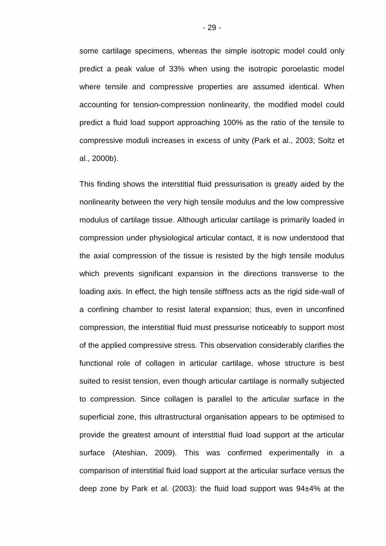
This finding shows the interstitial fluid pressurisation is greatly aided by the
nonlinearity between the very high tensile modulus and the low compressive
modulus of cartilage tissue. Although articular cartilage is primarily loaded in
compression under physiological articular contact, it is now understood that
the axial compression of the tissue is resisted by the high tensile modulus
which prevents significant expansion in the directions transverse to the
loading axis. In effect, the high tensile stiffness acts as the rigid side-wall of
a confining chamber to resist lateral expansion; thus, even in unconfined
compression, the interstitial fluid must pressurise noticeably to support most
of the applied compressive stress. This observation considerably clarifies the
functional role of collagen in articular cartilage, whose structure is best
suited to resist tension, even though articular cartilage is normally subjected
to compression. Since collagen is parallel to the articular surface in the
superficial zone, this ultrastructural organisation appears to be optimised to
provide the greatest amount of interstitial fluid load support at the articular
surface (Ateshian, 2009). This was confirmed experimentally in a
comparison of interstitial fluid load support at the articular surface versus the
deep zone by Park et al. (2003): the fluid load support was 94±4% at the

- 30 -
articular surface, but only 71±8% at the deep zone of immature bovine in
articular cartilage.
Cohen et al. (1998) employed transverse isotropy to approximate the
tension-compression nonlinearity for unconfined compression of in articular
cartilage plugs (Table 1.4) where the tissue is in tension in the transverse
plane (within which the modulus is high), and in compression in the axial
direction (along which the modulus is significantly lower). This model
considers cartilage depth-wise homogeneous and indirectly simulates the
different properties in tension and compression, although it does provide
better curve-fits of the experimental data than the linear biphasic poroelastic
model in cartilage modelling (Cohen et al., 1998).
Table 1.4 Transversely isotropic biphasic properties of bovine distal ulnargrowth plate and chondroepiphysis obtained from confined andunconfined compression tests (means ± std. dev.): (a) elastic moduli;(b) permeability coefficients (Cohen et al. 1998)
(a)E3[MPa]
compressionE1[MPa]tension
v21 v31
Growth plate 0.47 ±0.11 4.55 ±1.210.30±0.20
0.0
Chondroepiphysis 1.07 ± 0.27 10.63 ± 2.720.30±0.26
0.0
(b)k3 axial
[×10−15m4/(Ns)]k1 radial
[×10−15m4/(Ns)]n/a n/a
Growth plate 3.4 ± 1.6 5.0 ± 1.8 n/a n/a
Chondroepiphysis 2.1 ± 1.0 4.6 ± 2.1 n/a n/a
When Bursac et al. (1999) tested the same cartilage samples in confined
compression, measuring the radial normal stress on the confining chamber’s
side wall; they found stress magnitudes two to three times smaller than

- 31 -
predicted by the transversely isotropic model. This pointed out the limitation
of simulating tension-compression nonlinearity with transverse isotropy.
1.4.3 The microstructural FE models of articular cartilage
1.4.3.1 The fibril-reinforced poroelastic model
In order to overcome the limitation of transversely isotropic poroelastic
model on simulating tension-compression nonlinearity of articular cartilage,
the fibril-reinforced models are used. In these models, the fibril network
(collagen network) contributes to the mechanical stiffness of the material, in
addition to the isotropic matrix. The total solid stress σt of the fibril-reinforced
material is given by the sum of the matrix stress σm and fibril stress σf i.e.
σt = σm + σf. By defining the nonlinearly viscoelastic, direction and location
dependent mechanical properties of collagen fibrils, the anisotropy caused
by the collagen network and flow-independent viscoelasticity of articular
cartilage can also be included (Li et al., 2009).
Similar to the isotropic models, the nonlinearly viscoelastic equations of the
mechanical properties of collagen fibrils in the fibril-reinforced models are
also derived from the equations for the solid material. These equations, such
as Fung’s quasi-linear viscoelasticity (Fung, 1993, Section 7.6, Page 277-
279), extend elastic formulations by incorporating the reduced relaxation
functions G(t) - a normalized function of time (Fung 1993, Page 280). The
relaxation functions can effectively convert constant elastic moduli (e.g., λ
and μ) into functions of time t. Isotropic symmetry is assumed normally so
that the tensile stress in a cylindrical specimen under an infinitesimal stretch
(small deformation), at time t with the superposition principle applies (Fung

- 32 -
1993, Page 278-279), may be presented in the form of a convolution integral
(Fung 1993, Page 279):
(ݐ) = ()(0 (ݐ)ܩ(+ + න −ݐ)ܩ )∂()[ߣ( )]
∂
௧
1.2
where the ‘elastic response’ T(e)(λ) is a function of λ (Fung 1993, Page
278) and λ named the ‘stretch ratio’ for one-dimensional specimen loaded in
tension (Fung 1993, Page 29); the ‘reduced relaxation function’ G(t) is
typically analyzed into exponential function of time (Fung 1993, Page 280)
which can be written as (Fung 1993, Page 283):
(ݐ)ܩ = 1 + ∫ ( )௧ ఛ/ஶ
൧1 + ∫ ( )
ஶ
൧
ଵ1.3
‘The continuous spectrum model described above can be replaced by a
discrete spectrum model based on a hypothetical combination of Kelvin's
standard viscoelastic discrete models (Puso et al., 1998). In this case, the
reduced relaxation function can be written as a series of combinations of the
discrete relaxation functions such as:
(ݐ)ܩ = ஶܩ + ∑ ܩேୀ ௧ ఔ/ 1.4

- 33 -
Here, G∞ = G(∞); Gi is the discrete moduli; iߥ is the discrete relaxation time.’ -
equivalence between the two previous equations requires G∞ = 1 (Suh et al.,
1998).
These equations are used to derive the contribution of the fibrillar cartilage
part to the Jacobian matrix [ܦ] which is demanded in the commercial FE
package ABAQUS (Dassault Systemes, Suresnes Cedex, France).
[ܦ] = ߪ߂ /ߝ߂ , where Δߪ are the stress increments and Δߝare the strain
increments at a specific iteration of simulation (Abaqus User Subroutines
Reference Manual 1.1.36 ‘‘UMAT”).
1.4.3.2 Comparison of various fibril-reinforced models
Four kinds of fibril-reinforced models i.e. spring model (Soulhat et al., 1999;
Li et al., 1999-2003), continuum model (Li et al., 2004 and 2009; Wilson et
al., 2004; 2005a; 2006 and 2007), nonlinear shell membrane element model
(Shirazi et al., 2005 and 2007) and rebar-based model (Gupta et.al., 2009)
can be found in the literature simulating confined compression (CC),
unconfined compression (UCC), indentation and swelling test (Table 1.5).

- 34 -
Table 1.5 Fibril-reinforced FE models of articular cartilage.
Authors Configurations Modelling details
Spring-based
models
Li etal.,1999
UCCNonlinear formulation;
homogeneous.Li et
al.,2000UCC
Depth-dependent materialproperties.
Li etal.,2001
UCC versusRelease
Unequal load increments.
Li etal.,2002
UCCHealthy and pathological
situation.
Li etal.,2003
UCC (Strain rateand amplitude
varying)High strain rates.
Korhonen etal., 2003
UCCMechanical behaviour of normal,
PG depleted and collagendegraded AC.
Continuumelementmodels
Li et al.,2004
UCC(large deformation)
Fibril reinforcement versus tissuevolume change; load sharingbetween solid matrix and fluidpressurization; comparison ofspring model and continuum
model.Li et
al.,2009UCC; CC;indentation
3D fibril orientation; split-linepattern.
Wilson etal., 2004;
Indentation; UCC;CC
Depth-dependent collagenorientation and the compression-
tension nonlinearity
Wilson etal., 2005a
UCC; CC;indentation and
1D-swelling tests
Depth-dependent collagenorientation and the compression-
tension nonlinearity; osmoticswelling and chemical expansion.
Wilson etal., 2006
UCC; CC;indentation; 1D-swelling tests.
New laws for viscoelasticbehaviour and permeability of
the collagen network.
Wilson etal., 2007
UCC and CC;indentation and
1D-swelling tests
Intra- and extra-fibrillar watercontent; influence of the solidfraction on the compressive
properties.Julkunen et
al., 2007and 2008
UCCRealistic collagen orientation
(using PLM and MRIrespectively).
Julkunen etal., 2010
UCC;CC;indentation (strain
rate varying).Fractional factorial design.
Membraneelementmodels
Shirazi etal., 2005
Indentation;UCC and CC
Individual adjustment of collagenvolume fraction and mechanical
properties.
Shirazi etal., 2008
IndentationHorizontal and vertical membrane
elements.
Rebar-basedmodel
Gupta et al.,2009
Nano indentationFrictionless, finite sliding contact;
evolving indenter surface fluidflow boundary condition.

The spring-
In spring-based models, fi
nodes of the elements and can only be represented in the direction of the
elements. The most sophisticated spring
those of Li et al.
modelled as an isotropic solid matrix containing fluid
entrapped by a fibrillar network (Figure1.
Figure1.12 Diagram of the model showing the isotropic matrix (containingpores) and the fibrils edirections (Li
The isotropic matrix with pore fluid is considered as poroelastic, where both
the solid and the fluid phases are assumed to be incompressible. These
fibrils have no resistance to com
compression is assumed to be zero. The effect of lateral deformation of
- 35 -
-based models
based models, fibrils are represented by springs between the
nodes of the elements and can only be represented in the direction of the
The most sophisticated spring-based fibril-reinforced models are
et al. (1999-2003). In their earlier models,
modelled as an isotropic solid matrix containing fluid
entrapped by a fibrillar network (Figure1.12).
Diagram of the model showing the isotropic matrix (containingpores) and the fibrils evenly distributed in the three orthogonaldirections (Li et al., 1999).
The isotropic matrix with pore fluid is considered as poroelastic, where both
the solid and the fluid phases are assumed to be incompressible. These
fibrils have no resistance to compression, i.e. the Young's modulus for
compression is assumed to be zero. The effect of lateral deformation of
brils are represented by springs between the
nodes of the elements and can only be represented in the direction of the
reinforced models are
2003). In their earlier models, the cartilage is
modelled as an isotropic solid matrix containing fluid-saturated pores
Diagram of the model showing the isotropic matrix (containingvenly distributed in the three orthogonal
The isotropic matrix with pore fluid is considered as poroelastic, where both
the solid and the fluid phases are assumed to be incompressible. These
pression, i.e. the Young's modulus for
compression is assumed to be zero. The effect of lateral deformation of

- 36 -
every single fibril is also neglected. The only fibril stress considered is the
tensile stress produced by stretching in the radial direction. This is a
reasonable approximation given the slenderness of the collagen fibrils and
their high stiffness in tension. Thus the fibrils employed in the model are
one-dimensional (1D) nonlinear structural elements which do not support
compression. An elastic theory applies to the fibril constituent while a
poroelastic theory is employed for the biphasic component (Li et al., 1999).
The displacements are interpolated at all nodes and are thus quadratic. The
pore pressure is interpolated at the four corner nodes only and thus gives a
bilinear variation within an element. On the other hand, the fibrils are
represented by a system of special springs which resist tension only. Vertical
springs are not necessarily presented when the contacts are non-adhesive,
since they will undergo compression and thus develop no stress (pre-
stresses are not considered due to lack of such data). The total stiffness of
the horizontal fibrils within one continuum element domain is distributed
between one longer and four shorter springs (Figure 1.13).

- 37 -
Figure 1.13 Mesh for the finite elements illustrating also the arrangement ofspring elements in a porous continuum element. Displacements areinterpolated by all nodes, but the pore pressure is interpolated by fourcorner nodes only (Li et al., 1999).
It is assumed that the longer spring shares 2/3 of the total stiffness in order
to guarantee a uniform stress state when a uniform strain is produced. The
stiffness of the vertical springs can be determined in a similar way (Li et al.,
1999).
Using spring elements is an effective and economical method to represent
the fibrillar matrix of articular cartilage in finite-element computational
modelling. The spring-based fibril-reinforced biphasic models have been
applied in unconfined compression, mainly for the characterization of the
role of the collagen network in cartilage time-dependent response (Soulhat
et al., 1999 and Li et al., 1999-2003). The most significant difference

- 38 -
between the spring-based fibril-reinforced and the transversely isotropic
model is that the fibrils in the first model resist only tension, while the second
one has the same stiffness in compression and tension.
The continuum fibril-reinforced model
In the spring-based fibril-reinforced biphasic models, the standard porous
element was adopted for the non-fibrillar matrix containing fluid; and the
fibrillar matrix was discretised into two-node spring elements that were
attached to the eight-node porous elements. This leads to the deformation
incompatibility between the discretised matrices, and thus the validity of the
discretisation. Therefore, a user-defined continuum element was introduced
for the fibrillar matrix embedded in each porous element. Both the non-
fibrillar and the fibrillar part of the solid matrix were included in one
continuum element. The fibrillar continuum element shares the same nodes
and geometry with the corresponding porous element. So this approach
does not result in deformation incompatibility between the discretised
matrices (Li et al., 2004).
The continuum fibril-reinforced poroviscoelastic (FRPVE) models of Wilson
et al. (2004 and 2005a) include depth-dependent collagen orientation and
takes into account the compression-tension nonlinearity of AC. The primary
collagen fibrils were assumed to be viscoelastic and were represented by a
linear spring with stiffness E0, parallel to a nonlinear spring with stiffness E1
= Eε × εf (Eε is a positive material constant and εf is the fibril strain) in series
with a linear dashpot with damping constant η. The FRPVE model was
successfully used to describe confined compression, unconfined
compression and indentation (Wilson et al., 2004 and 2005a).

- 39 -
To account for the transient behaviour as well, the composition-based model
(Wilson et al., 2007) must be extended to include viscoelastic behaviour. It
was combined with the FRPVE model and expanded with a new
permeability law and a new law for the viscoelastic behaviour of collagen
network. The new permeability law is based on the assumption that both the
depth- and strain-dependencies of the permeability are governed by the
same mechanism and are the direct result of the composition of the tissue.
The combined model could simultaneously describe the behaviour of
articular cartilage in confined compression, unconfined compression,
indentation and two different 1D-swelling tests (Wilson et al., 2006).
In order to set up the sample-specific FE models, Julkunen et al. (2007)
derived specific collagen orientation patterns from quantitative microscopic
analyses and depth-wise T2 profiles (Julkunen et al., 2008), then
implemented realistic collagen architecture into the depth-dependent FRPVE
model (Wilson et al., 2004 and 2005a). The implementation of collagen
orientation into the FRPVE model enabled more realistic estimation of the
spatial, depth-dependent stress and strain distribution in articular cartilage,
as compared to models with homogeneous fibril distribution (Korhonen et al.,
2003 and Li et al., 1999).
Recently, Li et al. (2009) and Pierce et al. (2010) successfully implemented
the realistic orientation of collagen fibril into the fibril-reinforced continuum
models. The fibril orientation was derived by the split-pattern and Diffusion
Tensor (DT) Magnetic Resonance Imaging (MRI) method respectively.
Generally speaking, the discrete model with the fibrillar spring system
appeared to be slightly stiffer than the model consisting of continuum

- 40 -
elements only due to the deformation incompatibility between the discretised
matrices, especially at larger strains (Li et al., 2004).
The membrane shell element model
Neither the spring-based nor the continuum fibril-reinforced model explicitly
accounts for the important physical properties of the tissue, such as
nonlinear stress–strain curves of the fibril networks at different locations and
directions. To modify these models, Shirazi et al. (2005 and 2007) used
membrane shell elements to directly represent fibril network in both
axisymmetric and 3D model studies.
In the nonlinear membrane element fibril-reinforced model, the solid isotropic
porous matrix of the cartilage filled with water is represented, in a 3D mesh,
by 8-node or 20-node elements with regular or reduced integrations. The
pressure field is taken linear in different directions while the displacement
fields are either linear or quadratic. The fibrils are introduced by four-node or
eight-node shell membrane elements with, respectively, linear and quadratic
displacement fields. The collagen fibrils in the plane of membranes are
assumed to be homogeneously distributed in all directions.
Despite such distribution, a direction-dependent response prevails due to the
strain-dependency in the fibrils material properties and anisotropy in the
strain field. At each step of loading, principal strain directions in the plane of
membranes are taken as the material principal axes. The stresses in these
principal directions are subsequently evaluated based on the total principal
strains (Figure1.14) and fibrils stress–strain curve (Haut et al., 1972; Morgan
1960). Equal principal strains would generate an isotropic material modulus
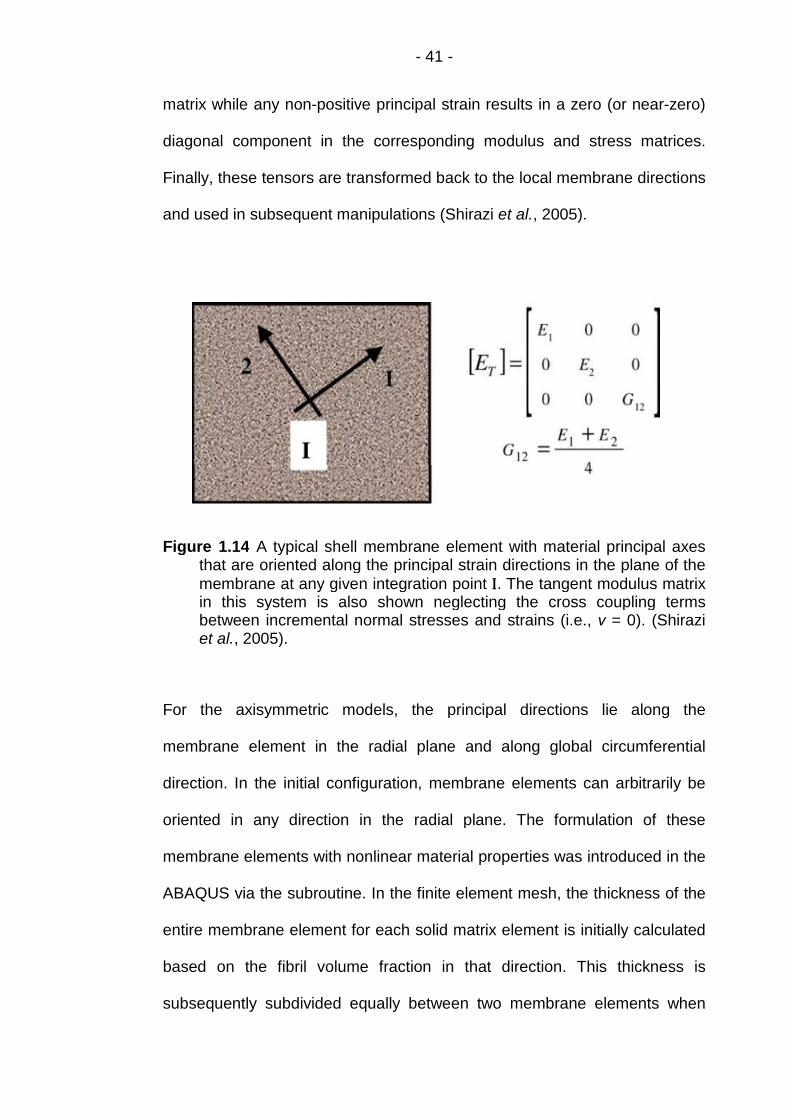
- 41 -
matrix while any non-positive principal strain results in a zero (or near-zero)
diagonal component in the corresponding modulus and stress matrices.
Finally, these tensors are transformed back to the local membrane directions
and used in subsequent manipulations (Shirazi et al., 2005).
Figure 1.14 A typical shell membrane element with material principal axesthat are oriented along the principal strain directions in the plane of themembrane at any given integration point I. The tangent modulus matrixin this system is also shown neglecting the cross coupling termsbetween incremental normal stresses and strains (i.e., ν = 0). (Shiraziet al., 2005).
For the axisymmetric models, the principal directions lie along the
membrane element in the radial plane and along global circumferential
direction. In the initial configuration, membrane elements can arbitrarily be
oriented in any direction in the radial plane. The formulation of these
membrane elements with nonlinear material properties was introduced in the
ABAQUS via the subroutine. In the finite element mesh, the thickness of the
entire membrane element for each solid matrix element is initially calculated
based on the fibril volume fraction in that direction. This thickness is
subsequently subdivided equally between two membrane elements when

using solid elements with linear displacement fields, or with proportions of
2/3 for the middle element and 1/6 for the side elements when considering
solid elements with quadratic
2005).
Figure 1.15 Finite element mesh of the model showing the arrangement ofhorizontal and vertical membrane elements in a typical axisymmetricporous continuum element
The rebar-based fibril
Prior fibril-reinforced
elements (Soulhat
elements (Shirazi
continuum elements (Wilson
- 42 -
using solid elements with linear displacement fields, or with proportions of
/3 for the middle element and 1/6 for the side elements when considering
solid elements with quadratic displacement fields (Figure1.15
Finite element mesh of the model showing the arrangement ofnd vertical membrane elements in a typical axisymmetric
porous continuum element (Shirazi et al., 2005).
based fibril-reinforced model
reinforced models have represented fibres as 1D nonlinear spring
elements (Soulhat et al., 1999 and Li et al.,1999-2003), 2D membranes
elements (Shirazi et al., 2005 and 2007), and user defined embedded
continuum elements (Wilson et al., 2004 and Li et al., 2
using solid elements with linear displacement fields, or with proportions of
/3 for the middle element and 1/6 for the side elements when considering
displacement fields (Figure1.15 Shirazi et al.,
Finite element mesh of the model showing the arrangement ofnd vertical membrane elements in a typical axisymmetric
models have represented fibres as 1D nonlinear spring
2003), 2D membranes
defined embedded
2009). Unlike all of

- 43 -
those models, the fibrillar collagen component was introduced by Gupta et
al. (2009) as 1D rebar elements embedded into the non-fibrillar proteoglycan
matrix. Rebar elements have two geometric properties: orientation angle and
cross-sectional area, both of which determine the volume fraction of fibres in
the model. To model the tension-compression nonlinearity of the collagen
fibres and the collapse of the fibres in compression, the individual rebar
elements resisted only tensile stresses. The dimension of the cartilage
surface elements was 1% of the indenter radius to ensure an accurate
computation of the contact area.
1.4.3.3 Comparison of element types used in fibril-reinforced FE
models
Deferent types of elements used in fibril-reinforced FE models implementing
collagen fibril direction are compared and the results are displayed in Table
1.6.

- 44 -
Table 1.6 Comparison of different element types to implement collagen fibrildirection in fibril-reinforced FE models:
ElementType
Author
Model Details
Definition offibril
directionMethod toimplement
Pros Cons Potentials
1D RebarGuptaet al.,2009
Oriented at00, ±300,
±600 from r,z and θ axes.
Embedded element
Thesimplestmodelwithout
subroutine.
Unrealisticfibril
direction.
Defineprincipal
eigenvectoras rebarelement.
2DContinuum
Wilsonet al.,2004
Arcademodel*.
UMAT3D
architecture of fibrils;
Only bevalid incentralpart ofload
bearingcartilage.
3D
Continuum
L. P. Li
et al.,
2009
Split-line
pattern.UMAT
Realisticorientation
ofcollagenfibril in
superficiallayer.
Fibrildirectionin deeplayers
may notbe sameas split-
line.
Split-line indeep layers;
oreigenvector
in wholecartilage.
3DContinuum
(Brick)
Pierceet al.,2010
Eigenvectorof DT-MRI
(corresponding to the
firstprincipal
eigenvalue).
Convexstrain-energyfunction
Ψ.
Estimatefibril
principaldirections
anddispersion
directlyfrom DT-MRI data.
ThesoftwarepackageFEAP is
notavailable.
Evaluatecartilagematrix
integrity(inAbaqus).
* Benninghoff (1925)
1.4.3.4 Methods to define collagen fibril orientation
As mentioned in Table 1.6, various patterns were used to define collagen
fibril orientation in different fibril-reinforced FE models. The detailed methods
are introduced below:

- 45 -
Method of rebar element
In the 2D axisymmetric fibril-reinforced FE model of Gupta et al. (2009),
rebar element was used to model the tension-compression nonlinearity of
the randomly oriented collagen fibrils in young porcine costal cartilage. The
individual rebar elements could only resist tensile stress. The random fibril
distribution was mimicked through fifteen different fibril orientations: Fibrils
were oriented at 0˚, ±30˚ and ±60˚ from the radial (r), axial (z) and
circumferential (θ) axes - six directions in each coordinate plane and totally
fifteen directions as each coordinate axis was used twice in different plane
(Figure 1.16).
Figure 1.16 The porous, nonfibrillar matrix of cartilage is represented with2D pore pressure elements and the randomly distributed collagen fibrilsare modeled with 1D embedded rebar elements oriented in 15 differentdirections at 0˚, ±30˚ and ±60˚ from the r, z and θ axes (Gupta et al., 2009).

- 46 -
Method of arcade model
Wilson et al. (2004) implemented the orientation of both the primary and the
secondary collagen fibril in their 2D axisymmetric fibril-reinforced
poroviscoelastic model using continuum elements.
According to the arcade model of Benninghoff (1925), the 3D collagen
network was captured as a combination of large primary collagen fibrils and
smaller secondary fibrils.
The primary collagen fibril bundles extend perpendicularly from the
subchondral bone, splitting up close to the articular surface into fibrils which
curve to a horizontal course. Each vertical bundle was assumed to split up in
four different fibril directions, curving in radial and circumferential directions
(Figure 1.17).
In the deep zone, the average angle of the primary fibrils with respect to the
r-axis as implemented in the FE model was 90˚. In the middle and superficial
zone this angle decreased to become zero at the articular surface.

- 47 -
Figure 1.17 Orientation of the primary fibrils as a function of depth. Right:cartoon of the arcade model of Benninghoff (1925). Left: Orientation offour primary collagen fibrils as implemented in the model (Wilson et al.,2004).
The orientation of the secondary fibrils was assumed to be random
(Benninghoff, 1925). The network of secondary fibrils was represented by a
relatively homogeneous 3D network of fibrils, running in the r-, θ- and z-
directions, in the bisector of the coordinate planes and in all directions with
equal angles with respect to the r-, θ-and z-axis - totally 13 different
orientations of the secondary fibrils at every integration point (Figure 1.18).
Secondary fibrils are relatively short and provide an extra matrix stiffness in
the corresponding direction.

- 48 -
Figure 1.18 Schematic representation of the 13 different orientations of thesecondary fibrils at any arbitrary point in the fibrillar matrix (Wilson etal., 2004).
Method of split-pattern
Although the two methods can implement collagen fibril orientation to the
fibril reinforced models, the orientations used are idealised without detailed
realistic information from experiments. The split-pattern method introduced
in Section 1.3 has been used to derive the realistic fibril orientation (Figure
1.19) in Li et al. (2009).
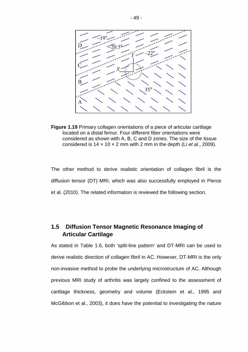
- 49 -
Figure 1.19 Primary collagen orientations of a piece of articular cartilagelocated on a distal femur. Four different fiber orientations wereconsidered as shown with A, B, C and D zones. The size of the tissueconsidered is 14 × 10 × 2 mm with 2 mm in the depth (Li et al., 2009).
The other method to derive realistic orientation of collagen fibril is the
diffusion tensor (DT) MRI, which was also successfully employed in Pierce
et al. (2010). The related information is reviewed the following section.
1.5 Diffusion Tensor Magnetic Resonance Imaging of
Articular Cartilage
As stated in Table 1.6, both ‘split-line pattern’ and DT-MRI can be used to
derive realistic direction of collagen fibril in AC. However, DT-MRI is the only
non-invasive method to probe the underlying microstructure of AC. Although
previous MRI study of arthritis was largely confined to the assessment of
cartilage thickness, geometry and volume (Eckstein et al., 1995 and
McGibbon et al., 2003), it does have the potential to investigating the nature

- 50 -
of fluid dynamics in AC through its ability to distinguish between moving and
stationary fluids (Callaghan et al., 1991).
1.5.1 Diffusion tensor magnetic resonance imaging (DT-MRI)
In the mid-1980s, the basic principles of DT-MRI were combined with MR
imaging principles to encode molecular diffusion effects in the MR signal
(Bihan et al., 1985; Merboldt et al., 1985 and Taylor et al., 1985). Molecular
diffusion refers to the random translational motion of molecules resulting
from the thermal energy carried by these molecules. During their random
diffusion-driven displacements, molecules probe tissue structure at a
microscopic scale well beyond the usual image resolution: during typical
diffusion times of about 50 msec, water molecules move in articular cartilage
bouncing, crossing, or interacting with many tissue components such as
fibers or macromolecules (Denis et al., 2001). This made DT-MRI the only
means to observe diffusion in vivo noninvasively accompanying access to
both superficial and deep organs with high resolution.
Diffusion is expected to be anisotropic in the structurally aligned collagen
fibrillar architecture of AC (Jeffery et al., 1991), the self-diffusion of the water
molecules can therefore only be fully characterized in terms of a 3 3
diffusion tensor describing both the magnitude and direction of the diffusion
in 3-dimensional space (Basser et al., 1994).
1.5.2 The primary collagen orientation of articular cartilage
Meder et al. (2006) and Filidoro et al. (2005) suggested that the principal
eigenvectors (corresponding to the maximum eigenvalue) of the water
diffusion tensor follow the collagen fibre directions: On the timescale of the
DT-MRI measurements, water molecules diffuse over distances of a few

- 51 -
microns (Meder et al., 2006), which is much larger than the diameter (~ 40
nm) of the collagen fibrils themselves (Langsjo et al., 1995). Consequently
the diffusion of water in cartilage is restricted by the presence of the collagen
fibre bundles. This restriction is greatest in a direction normal to the fibres,
leading to a lower diffusivity in this direction and a correspondingly higher
diffusivity parallel to the direction of the local fibre orientation.
The principal eigenvector can be represented by a “quiver” plot, where each
quiver represents the projection of the principal diffusion eigenvector on to
the image plane. For each pixel of the DT-MRI grid, the principal eigenvector
was projected to one of the global planes. Then all of the projections in the
same plane were attached on the bottom of the corresponding pixel to
create the 2D quiver plot. The 2D quiver plot of the collagen fibril derived by
Meder et al. (2006) is displayed in Figure 1.20.
Figure 1.20 2D quiver plots of the collagen fibril, (a) before compression andafter two subsequent compressions (b) by 18% and (c) by 29% of theoriginal cartilage thickness, respectively (Meder et al. 2006).
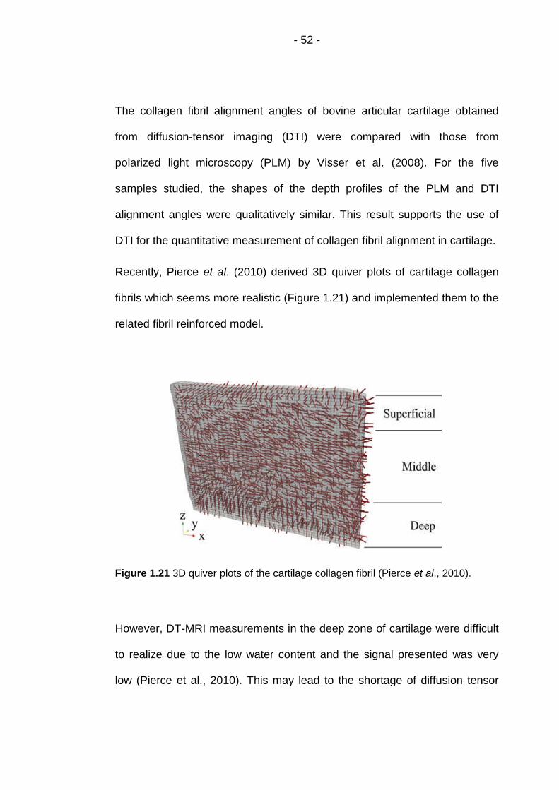
- 52 -
The collagen fibril alignment angles of bovine articular cartilage obtained
from diffusion-tensor imaging (DTI) were compared with those from
polarized light microscopy (PLM) by Visser et al. (2008). For the five
samples studied, the shapes of the depth profiles of the PLM and DTI
alignment angles were qualitatively similar. This result supports the use of
DTI for the quantitative measurement of collagen fibril alignment in cartilage.
Recently, Pierce et al. (2010) derived 3D quiver plots of cartilage collagen
fibrils which seems more realistic (Figure 1.21) and implemented them to the
related fibril reinforced model.
Figure 1.21 3D quiver plots of the cartilage collagen fibril (Pierce et al., 2010).
However, DT-MRI measurements in the deep zone of cartilage were difficult
to realize due to the low water content and the signal presented was very
low (Pierce et al., 2010). This may lead to the shortage of diffusion tensor

- 53 -
measurements in the deepest part of the cartilage sample. Due to the image
noise, the length of the MRI pixel grids may also be shorter than the sample.
1.6 Summary of the literature review
In order to gain better understanding of fundamental lubrication mechanism
of articular cartilage, the related literature on cartilage biomechanics and
lubrication were reviewed, followed by the review of the related
computational models and the brief introduction on DT-MRI.
Implementing the realistic collagen fibril orientation derived from DT-MRI
data, the fibril-reinforced model of Pierce et al. (2012) is the most realistic,
comparing to the others with idealized (Gupta et al., 2009) or simplified fibril
orientation (Li et al., 2009 and Rasanen et al., 2012). However, the model in
Pierce et al. (2012) did not include viscous effects in both the solid matrix
and the fibril. In order to set up the more realistic fibril-reinforced model, it is
necessary to employ the material model of Li et al., 2009 and implement the
collagen fibril orientation defined by DT-MRI data as Pierce et al. (2012) did.
1.7 Project Aims and Objectives
Rationale:
The effect of composition and structure of articular cartilage, particularly the
realistic collagen fibril orientation, on fluid load support have not been
investigated in details. This provides an ideal opportunity to develop the
computational models incorporating FE analysis and DT-MRI data to present
a better understanding of fundamental lubrication mechanism of articular
cartilage.
- 54 -
Aims:
The aim of this project is to develop more realistic fibril-reinforced
computational models that incorporate FE analysis and DT-MRI data, with
the better interpretation of interstitial fluid pressure and load support in
cartilage.
Objectives:
1) To set up an isotropic poroelastic FE model to predict fluid load
support in cartilage.
2) To provide the more detailed analysis of the collagen fibril orientation
defined by the principal eigenvector of diffusion tensor, in contrast to
the literature, and verify the rationality of the definition.
3) To develop the method to implement DT-MRI data in the fibril-
reinforced models.
4) To set up the 2D fibril-reinforced poroelastic models implementing
DT-MRI data and “user material” option in ABAQUS to overcome the
limitation of previous models; compare the results with (1).
5) To extend the 2D fibril-reinforced model to 3D one to predict fluid load
support in articular cartilage.
6) To simulate the model with experimental results using the 3D model,
and validate the feasibility and reliability of the methodologies to
implement the DT-MRI data to the fibril-reinforced models.

- 55 -
Chapter 2 Analysis of Diffusion Tensor Magnetic Imaging
Data
2.1 Introduction
In articular cartilage, water molecules diffuse over distances of a few
microns which are much larger than the diameter (~ 40nm) of the collagen
fibrils (Langsjo et al., 1995). Consequently the diffusion of water in cartilage
is restricted by the presence of the collagen fibre bundles. This restriction is
greatest in a direction normal to the fibres, leading to a lower diffusivity in
this direction and a correspondingly higher diffusivity parallel to the direction
of the local fibre orientation (Meder et al., 2006 and Filidoro et al., 2005).
High resolution DT-MRI provides the detailed information of water and water
flow (Visser et al., 2008), as well as the composition and structure of
articular cartilage. Once a DT is derived in terms of a 3 3 matrix for each
pixel grid of MRI, its eigenvalues and the corresponding eigenvectors can be
calculated by diagonalizing the matrix. The eigenvectors are independent of
the scanner coordinates, representing the three principal directions of this
DT and their magnitudes within the tissue. The principal eigenvector
corresponding to the maximum eigenvalue of a DT follows the direction of
the collagen fibril within the corresponding MRI pixel grid (Meder et al., 2006
and Filidoro et al., 2005).
In order to verify the rationality of the DT-MRI data to represent the collagen
fibril orientation in articular cartilage, their relationship is introduced first in
this chapter; and the methods to analyze the DT-MRI data, the results of the

- 56 -
analysis and the discussion of the results are also described. The
information on the direction of the fibres was then used in Chapter 3 to
determine the material model.
The first section of the chapter introduces the definition of the orientation of
the collagen fibril using DT-MRI results, together with the two kinds of
method to analyze the DT-MRI data. The detailed analysis results of the DT-
MRI data is presented in the second section. The last section discusses the
DT-MRI results and verifies its consistency with the literature. The rationality
to implement the DT-MRI data to the FE models representing the collagen
fibril orientation is also verified in the mean time.
2.2 Method to Analyze the DT-MRI Data
2.2.1 Material
A high resolution 9.4T DT-MRI was performed by Dr Robin Damion (School
of physics, University of Leeds), on the cross-section of a cylindrical articular
cartilage specimen (through the symmetric axis) with 6.0 mm diameter and
1.36 mm thickness (Fermor et al., 2013; Figure 2.1). Specimens were
collected from the patellofemoral grooves of an 18 month old bovine knee
joints (stored frozen in Ringer’s solution and used within a month of
collection).
Z

- 57 -
Figure 2.1 Schematic diagram of cartilage speciThe Y-axis was defined as into page perpen(Modified from Pierce et al., 2010).
2.2.2 The Diffusion Tensor MRI scann
The MRI image resulting from the scan of the a
dimensional image consisting of 17 rows and 74
and the horizontal resolutions were 70μm. As pa
diffusion tensor was derived for each pixel within
dimension of the pixel grid did not exactly m
cartilage sample in Figure 2.1 due to the lim
Chapter 1, Section 1.5): the thickness and leng
(17 × 0.07) mm and 5.18 (74 × 0.07) mm respec
was derived corresponding to the deepest and si
The principal eigenvectors (unit vectors) of
presented as components along three globa
(ଶ +
ଶ + ଶ = 1) where i = 1∙∙∙17 from to
and j = 1∙∙∙74 from left to right respectively.
X
1.36mm D6mm
men scanned using MRI.dicular to the X and Z axes
ing and pixel definitions
rticular cartilage was a two-
columns. Both the vertical
rt of the DT-MRI process, a
the image. Please note the
atch the geometry of the
itation of the DT-MRI (See
th of the pixel grid was 1.19
tively i.e. no diffusion tensor
de part of cartilage.
DT were calculated and
l axes i.e. , and
p to bottom of the pixel grid

- 58 -
2.2.3 Method for analysing the principal eigenvectors
The DT-MRI data particularly the principal eigenvectors were analysed
through two steps using different method: the direct observation of 2D quiver
plot and the quantitative analysis by calculating the angle between the
principal eigenvector and the X-Y plane parallel to the cartilage surface in
each pixel of MRI.
2.2.3.1 The 2D quiver plots
The first step of analysing the principal eigenvectors was to look for the
distribution of collagen fibril visually through direct observation of the 2D
quiver plots of eigenvector components on the global coordinate planes
(totally three plots). The 2D quiver plot was made of the projection of the
principal eigenvectors: for each pixel of the DT-MRI grids, the principal
eigenvector was projected to one of the global planes. Then all of the vector
components in the same plane were attached on the bottom of the
corresponding pixel to create the 2D quiver plot.
These plots allow qualitative analysis of the distribution of collagen fibril. For
the convenience of interpretation, the quiver plot in the X-Z plane was
selected. The length of the quiver, i.e. ටଶ +
ଶ , has an important hint:
its increase means the decrease of and indicates the decrease of the
angle between the quiver and the X-Z plane. So the long quiver (tends to be
1) in the X-Z plane means the corresponding principal eigenvectors nearly
parallel to the X-Z plane; hence the direction of the long quiver can nearly
represent the angle between the corresponding eigenvector and the
cartilage surface which parallel to the X-Y plane. However, the short quivers

- 59 -
can only partly show the angle between the principal eigenvectors and the
cartilage surface. To solve this problem, the exact value of the angle
between the principal eigenvector and the cartilage surface should be
calculated for each pixel of MRI.
2.2.3.2 Analysis of the angles between the principal
eigenvectors and the cartilage surface
The second step of analysing the principal eigenvectors was to study the
distribution of the fibril by calculating the angles ߚ (0°≤ ≥ߚ 90°; i and j
represents the row and column number of the corresponding pixel
respectively) between the principal eigenvectors and the X-Y plane parallel
to the cartilage surface. ߚ was defined as:
ߚ = tanଵ ቤ /ටଶ +
ଶ ቤ …………………. (2.1)
where , and are the components of the corresponding
principal eigenvector on the three global axes respectively.
The angle ߚ is extremely important in modelling cartilage particularly in the
surface zone, as it directly affects the horizontal component value of the fibril
tensile stress on the corresponding site of cartilage. As introduced in Section
1.4.2.2, the horizontal tensile stress can prevent lateral expansion of
cartilage and enhance the pressurization of interstitial fluid to support the
applied load.

- 60 -
The fibril angles in the same row were gathered in one bar chart to observe
the layered distribution of collage fibril in the tissue and compared with the
quiver plot, totally 17 bar charts were produced.
Then the percentage occupied by every 10 degree of fibril angle in the same
layer was calculated and displayed by the x-y scatter (each interregional
represented by the upper limit). Then the scatters with similar trend were put
together to find out the layered fibril angle distribution quantitatively.
2.3 Results
2.3.1 Two-dimensional quiver plots
A two-dimensional quiver plot in the X-Z plane of the principal eigenvectors
of the whole cartilage sample cross-section is shown in Figure 2.2 (provided
by Dr Robin Damion), with the row and column numbers displayed on the
vertical and horizontal axis respectively.

- 61 -
Figure 2.2 X-Z components of principal eigenvector of diffusion tensor. (Zaxis shows the row number, and X axis shows the column number ofthe pixel grid; provided by Dr Robin Damion)
In Figure 2.2, most fibril components in the top 2 layers (0.14 mm thick) of
the pixel grids which occupied 10.0% of cartilage sample thickness tended to
be horizontal. In the next seven layers (the 3rd - 9th layer) occupying 36.0%
of cartilage thickness, fibril components showed various gradients and no
single gradient was found to be dominant, i.e. fibrils distributed randomly. In
the remaining layers (the 10th-17th layer) occupying 41.2% of cartilage
thickness, most fibril components were or tended to be vertical (except in the
17th layer). This will be discussed in Section 2.4.
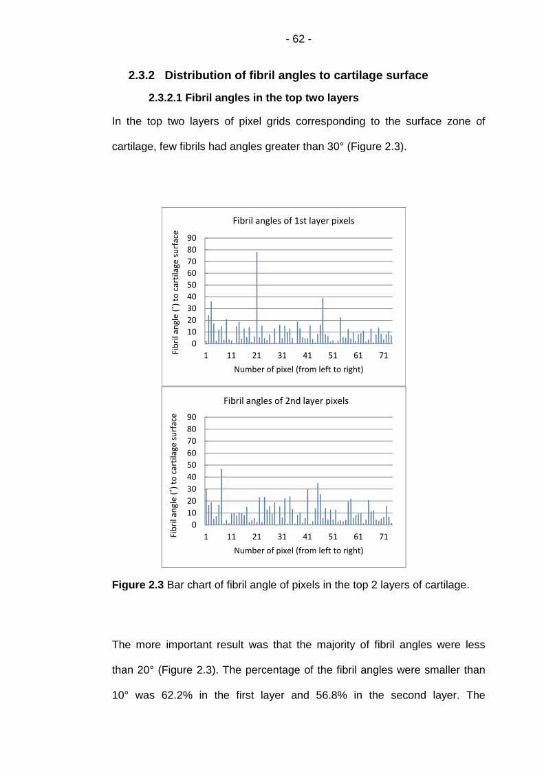
- 62 -
2.3.2 Distribution of fibril angles to cartilage surface
2.3.2.1 Fibril angles in the top two layers
In the top two layers of pixel grids corresponding to the surface zone of
cartilage, few fibrils had angles greater than 30° (Figure 2.3).
Figure 2.3 Bar chart of fibril angle of pixels in the top 2 layers of cartilage.
The more important result was that the majority of fibril angles were less
than 20° (Figure 2.3). The percentage of the fibril angles were smaller than
10° was 62.2% in the first layer and 56.8% in the second layer. The
0
10
20
30
40
50
60
70
80
90
1 11 21 31 41 51 61 71Fib
rila
ngl
e(˚
)to
cart
ilage
surf
ace
Number of pixel (from left to right)
Fibril angles of 1st layer pixels
0
10
20
30
40
50
60
70
80
90
1 11 21 31 41 51 61 71Fib
rila
ngl
e(˚
)to
cart
ilage
surf
ace
Number of pixel (from left to right)
Fibril angles of 2nd layer pixels

- 63 -
percentage less than 20° was 91.9% in the first layer and 85.1% in the
second layer respectively (Figure 2.4). Meanwhile, only a few fibril angles
were greater than 30°. This means most collagen fibrils in the first two layers
from the cartilage surface tended to be horizontal.
Figure 2.4 Fibril angle distribution of pixels in top 2 layers from cartilagesurface.
2.3.2.2 Fibril angles in layers from the 3rd to 9th
Fibril angles in the 3rd and 4th layer
Most of the fibril angles in the 3rd and 4th layer of pixel grids were less than
30° (Figure 2.5), 74.3% and 68.9% respectively (Figure 2.6).
0
10
20
30
40
50
60
70
80
90
100
0 10 20 30 40 50 60 70 80 90
Per
cen
tage
(%)
Fibril angle (˚) to cartilage surface
1st layer
2nd layer

- 64 -
Figure 2.5 Bar chart of fibril angle of pixels in the 3rd and 4th layer ofcartilage.
It seemed feasible to classify the two layers belonging to the surface zone of
the cartilage. But only 24.3% of the fibril angles were smaller than 10° in the
3rd layer and 23.0% in the 4th layer (Figure 2.6). Meanwhile, a number of
angles were greater than 40° (Figure 2.5 and 2.6). So it was more
reasonable for the two layers to be included in the middle zone of the
cartilage.
0
10
20
30
40
50
60
70
80
90
1 11 21 31 41 51 61 71
Fib
rila
ngl
e(°
)to
cart
ilage
surf
ace
Number of pixel (from left to right)
Fibril angle of 3rd layer pixels
0
10
20
30
40
50
60
70
80
90
1 11 21 31 41 51 61 71Fib
rila
ngl
e(°
)to
cart
ilage
surf
ace
Number of pixel (from left to right)
Fibril angle of 4th layer pixels
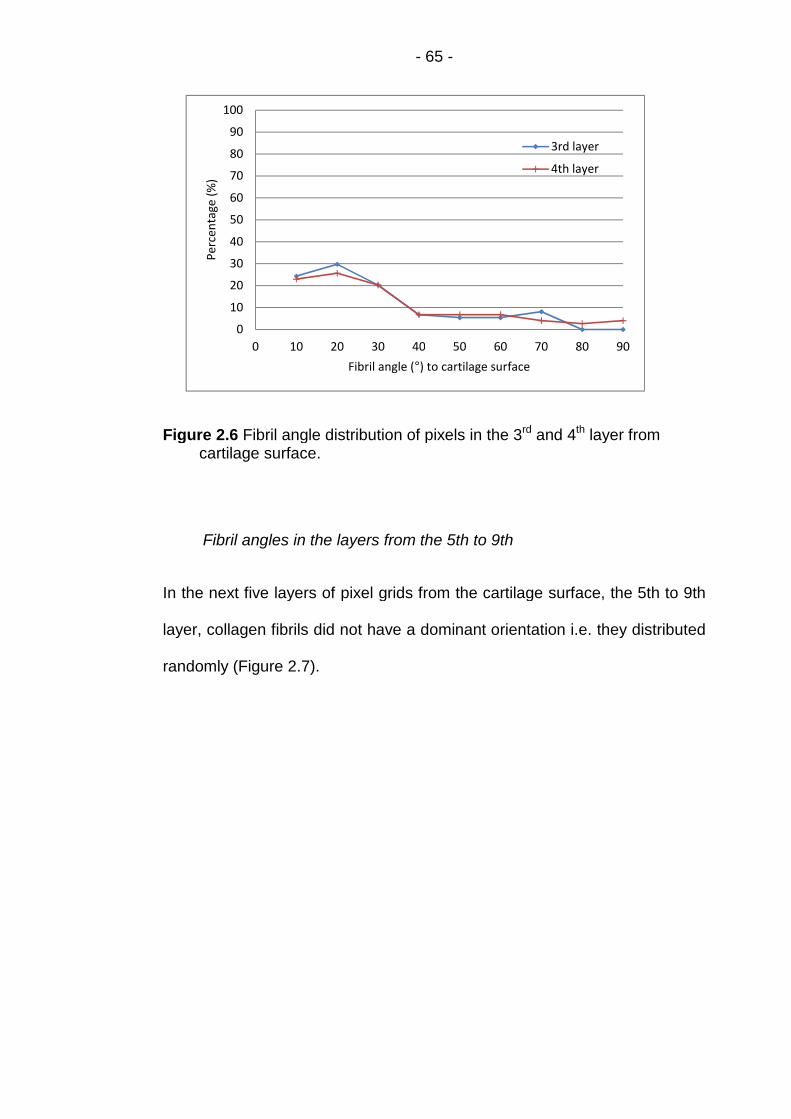
- 65 -
Figure 2.6 Fibril angle distribution of pixels in the 3rd and 4th layer fromcartilage surface.
Fibril angles in the layers from the 5th to 9th
In the next five layers of pixel grids from the cartilage surface, the 5th to 9th
layer, collagen fibrils did not have a dominant orientation i.e. they distributed
randomly (Figure 2.7).
0
10
20
30
40
50
60
70
80
90
100
0 10 20 30 40 50 60 70 80 90
Per
cen
tage
(%)
Fibril angle (°) to cartilage surface
3rd layer
4th layer
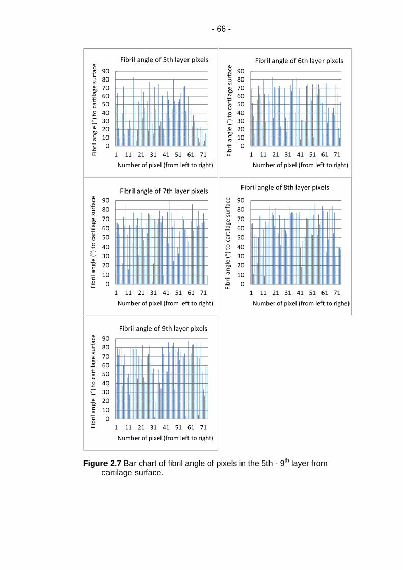
- 66 -
Figure 2.7 Bar chart of fibril angle of pixels in the 5th - 9th layer fromcartilage surface.
0102030405060708090
1 11 21 31 41 51 61 71Fib
rila
ngl
e(°
)to
cart
ilage
surf
ace
Number of pixel (from left to right)
Fibril angle of 5th layer pixels
0102030405060708090
1 11 21 31 41 51 61 71Fib
rila
ngl
e(˚
)to
cart
ilage
surf
ace
Number of pixel (from left to right)
Fibril angle of 6th layer pixels
0
10
20
30
40
50
60
70
80
90
1 11 21 31 41 51 61 71
Fib
rila
ngl
e(°
)to
cart
ilage
surf
ace
Number of pixel (from left to right)
Fibril angle of 7th layer pixels
0
10
20
30
40
50
60
70
80
90
1 11 21 31 41 51 61 71
Fib
rila
ngl
e(°
)to
cart
ilage
surf
ace
Number of pixel (from left to righe)
Fibril angle of 8th layer pixels
0
10
20
30
40
50
60
70
80
90
1 11 21 31 41 51 61 71Fib
rila
ngl
e(°
)to
cart
ilage
surf
ace
Number of pixel (from left to right)
Fibril angle of 9th layer pixels

- 67 -
In each of the layers from the 5th to the 9th, the percentage occupied by
each interregional (10°) of fibril angle was less than 30%; and the total
percentage occupied by fibril angles ≥ 60° (the sum of the values of the last
three points of each individual curve) was less than 60% (Figure 2.8). This
result confirmed the conclusion drawn from the angle bar charts in Figure
2.7 that the collagen fibrils distributed randomly. So all of the five layers
should be included in the middle zone of the cartilage.
Figure 2.8 Fibril angle distribution of pixels in the 5th - 9th layer fromcartilage surface.
0
10
20
30
40
50
60
70
80
90
100
0 10 20 30 40 50 60 70 80 90
Per
cen
tage
(%)
Fibril angle (°) to cartilage surface
5th layer
6th layer
7th layer
8th layer
9th layer

- 68 -
2.3.2.3 Fibril angles in layers from the 10th to 17th
Fibril angles in the layers from the 10th to 15th
In the layers from the 10th to the 15th of pixel grids corresponding to part of
the cartilage deep zone, lots of the percentage occupied by these fibril
angles ≥ 70° in most layers was greater than 60% (except 58.1% in the 15th
layer; Figure 2.9); and the amount of the fibrils with angle greater than 60°
increased apparently in comparison to the higher layers (Figure 2.10). This
result clearly showed most collagen fibrils in these layers tended to be
vertical, although several angles were less than 40° even less than 10°
(Figures 2.9 and 2.10).
Figure 2.9 Fibril angle distribution of elements in 10th - 15th layer fromcartilage surface.
0
10
20
30
40
50
60
70
80
90
100
0 10 20 30 40 50 60 70 80 90
Per
cen
tage
(%)
Fibril angle (°) in X-Z plane
10th layer
11th layer
12 layers
13th layer
14th layer
15th layer

- 69 -
Figure 2.10 Bar chart of fibril angle of pixels in the 10th - 15th layer fromcartilage surface.
0
20
40
60
80
1 11 21 31 41 51 61 71Fib
rila
ngl
e(°
)to
cart
ilage
surf
ace
Number of pixel (from left to right)
Fibril angle of 10th layer pixels
0
20
40
60
80
1 11 21 31 41 51 61 71Fib
rila
ngl
e(°
)to
cart
ilage
surf
ace
Number of pixel(from left to right)
Fibril angle of 11th layer pixels
0
20
40
60
80
1 11 21 31 41 51 61 71Fib
rila
ngl
e(°
)to
cart
ilage
surf
ace
Number of pixel (from left to right)
Fibril angle of 12th layer pixels
0
20
40
60
80
1 11 21 31 41 51 61 71
Fib
rila
ngl
e(°
)to
cart
ilage
surf
ace
Number of pixel (from left to right)
Fibril angle of 13th layer pixels
0
10
20
30
40
50
60
70
80
90
1 11 21 31 41 51 61 71
Fib
rila
ngl
e(°
)to
cart
ilage
surf
ace
Number of pixel (from left to right)
Fibril angle of 14th layer pixels
0
10
20
30
40
50
60
70
80
90
1 11 21 31 41 51 61 71
Fib
rila
ngl
e(°
)to
cart
ilage
surf
ace
Number of pixel(from left to right)
Fibril angle of 15th layer pixels

- 70 -
Fibril angles in the 16th and 17th layer
As a part of the deep zone, the fibril distribution seemed to be random in the
16th and 17th layer particularly in the 17th layer (Figure 2.11 and 2.12). The
reason led to the phenomenon is discussed in the following section.
Figure 2.11 Bar chart of fibril angle of pixels in the 16th and 17th layer fromcartilage surface.
0
10
20
30
40
50
60
70
80
90
1 11 21 31 41 51 61 71
Fib
rila
ngl
e(°
)to
cart
ilage
surf
ace
Number of pixel (from left to right)
Fibril angle of 16th layer pixels
0
10
20
30
40
50
60
70
80
90
1 11 21 31 41 51 61 71
Fib
rila
ngl
e(°
)to
cart
ilage
surf
ace
Number of pixel (from left to right)
Fibril angle of 17th layer pixels

- 71 -
Figure 2.13 Fibril angle distribution of elements in 16th and 17th layer fromcartilage surface.
2.4 Discussion
The orientation of collagen fibril was defined by the principal eigenvector of
the DT and projected visually on the plane of cartilage cross-section (X-Z
coordinates plane) as shown in Figure 2.2. The distribution of collagen fibril
in articular cartilage was largely consistent with the literature particularly the
results of Visser et al. (2008) which was also derived from DT-MRI data
(Figure 1.20a).
In the top two layers, most of the angles between the principal eigenvectors
and the planes parallel to the cartilage surface are less than 20° (Figure 2.4).
This result and the angle distribution in the deep zone of cartilage (Figure
2.9-2.10) were in agreement with Meder et al. (2006), which found “the
principal component of the diffusion tensor appears to be at around 75° to
0
10
20
30
40
50
60
70
80
90
100
0 10 20 30 40 50 60 70 80 90
Per
cen
tage
(%)
Fibril angle (°) to cartilage surface
16th layer
17th layer

- 72 -
the normal near the articular surface, while in the deep zone it appears to be
at approximately 20° to the normal.”. This confirms the direct observation of
Figure 2.2 in Section 2.3.2. The most important finding is that: these results
verified the rationality to implement the principal eigenvectors of DT in the
computational models representing the fibril orientation.
In the deepest area of cartilage (the eight layers in Figures 2.9 - 2.13), there
are a limited number of angles that were less than 40° (even than 10°) which
seems not consistent with the predominant view in the literature considering
all of the collagen fibrils perpendicular to the cartilage surface (Mow et al.,
1992). But Kaab et al. (1998) also had the similar finding as introduced in
Section 1.3: some fibrils run obliquely in the deep zone while the majority
collage columns are perpendicular to the cartilage surface (Figure 1.7b).
However, DT-MRI measurements in the deep zone of cartilage were difficult
to realize due to the low water content and the signal presented was very
low (Pierce et al., 2010). This led to the shortage of diffusion tensor
measurements in the deepest part of the cartilage sample in Figure 2.1, so
the thickness of the MRI pixel grids in Figure 2.2 was 0.17mm less
compared to the sample. The length of the MRI pixel grids was shorter
because of the image noise.
Visser et al. (2008b) explained the phenomenon that several angles are
greater than 50° in the top two layers: Fibres are disordered within a given
DTI pixel of a length scale of 10 μm and a particular water molecule can
access a range of fibre orientations on the timescale of a DTI measurement.
This resulted in the measured DT behaving as weighted average quantities.

- 73 -
But this limitation does not affect the fibril angles defined by the DT in other
pixels and the whole distribution of collage fibril in the specific layer.
As reviewed in Section 1.4 and 1.5, Pierce et al. (2010) had also derived the
orientation of collagen fibrils in bovine groove cartilage from DT-MRI data
and successfully implemented the fibril direction to their finite element
model. Different from the 2D quiver plot in this chapter, the 3D quiver plot
was used to display the fibril orientation.
From the theoretical mechanism to the clinical application and the practice of
computational modeling, the feasibility and rationality of the DT-MRI have
been fully proved. So the principal eigenvector will be defined as primary
collagen orientation and implemented to the 2D and 3D fibril-reinforced FE
models in the following chapters.

- 74 -
Chapter 3 Material Model and Method to Implement
DT-MRI Data
3.1 Introduction
This chapter describes the material model of cartilage employed in the finite
element analysis within this thesis, including how information from the DT-
MRI data (described in Section 2.2) was used to create local material
property variations which reflect the direct of reinforcing fibrils. As this work
includes both 2D axisymmetric and 3D models, the specific implementation
for each of those element types is described. This chapter is concerned
primarily with the Young’s modulus values assigned to the solid phase of the
cartilage and does not discuss any fluid behavior. In all cases it was
assumed that the cartilage solid phase is composed of a linear elastic matrix
and distribution of viscoelastic fibrils. Each of which has an individual
orientation. In order to include the effect of the fibrillar component it is
necessary to include a fibril direction for each element and a function to
calculate the viscoelastic property change as strain increases.
Section 3.2 gives the equations used to define the strain-dependent fibrillar
Young’s modulus. The time discretization scheme is shown, along with
simplifications which can be made when the instantaneous fibrillar modulus
was used. The material model derived here was implemented into a
FORTRAN subroutine, for using with ABAQUS, by Li et al (2009) which was
used in this thesis.
Sections 3.3 and 3.4 describe the implementation of the collagen fibril
direction in the 2D and 3D finite element models respectively. Details are

- 75 -
given of the commands used to import the primary fibril orientation
information (described in Chapter 2) and convert it into a local coordinate
system for each element in the model.
3.2 Material Model
In the fibril-reinforced FE models of this thesis, the material properties for
each element were modified based on the primary fibril orientation in that
area, using ‘‘user material” option i.e. ‘‘UMAT” in ABAQUS (Dassault
Systemes, Suresnes Cedex, France) - the FORTRAN written subroutine (Li
et al., 2009) was kindly provided by Dr L. P. Li, Calgary University of
Canada.
Articular cartilage can be considered as a porous matrix saturated in water,
reinforced by the fibrillar network. The porous matrix was nonfibrillar,
representing the solid matrix excluding the collagen fibers. The nonfibrillar
matrix was modeled as a continuous linearly elastic material, with the
Young’s modulus Em, and Poisson’s ratio νm. These basic properties were
augmented with representation of the fibrillar network, which was modeled
as nonlinearly viscoelastic, direction and location dependent properties.
‘Using ݔ to represent a fiber direction at a location with Cartesian
coordinates (X, Y, Z), the fibrillar modulus in the direction of ݔ is a function of
the tensile strain in the direction, ௫ܧ(ߝ௫ ), as well as a function of ݔ and (X, Y,
Z) (anisotropic and inhomogeneous). The fibrillar modulus was taken to be
zero for compressive strains. … Shear stress between parallel fibers was
neglected, but shearing was modeled in the nonfibrillar porous matrix.’ (Li et
al. 2009).

- 76 -
3.2.1 The Jacobian matrix of fibril-reinforced FE model
Jacobian matrix, defined as: [ܦ] = ߪ߂ /ߝ߂ was required to implement
material properties in the fibril-reinforced FE models, where Δߪ are the
stress increments and Δߝare the strain increments. This was achieved by
using ‘‘UMAT” available in ABAQUS (Abaqus User Subroutines Reference
Manual 1.1.36 ‘‘UMAT”). As only small deformation problems were solved,
the Jacobian matrix for the fibril-reinforced model of AC was:
[D] =
⎣⎢⎢⎢⎢⎡௫௫ܦߣߣ
ߣ௬௬ܦߣ
ߣߣ௭௭ܦ
000
000
000
000
000
000
ߤ00
0ߤ0
00⎦ߤ⎥⎥⎥⎥⎤
(3.1)
where λ and μ are the Lamé constants of the nonfibrillar matrix.
According to the biphasic theory, the stress of the fibril-reinforced material is
the sum of the matrix and fibril stresses. The nonfibrillar matrix was isotropic
with linearly elastic property, hence
௫௫ܦ = +ߣ +ߤ2 ௫ߪ߂ ௫ߝ߂
/ (3.2)
here ௫ߪ߂ ௫ߝ߂
/ represents the contribution of the fibrillar matrix to the
Jacobian and will be derived in the following section.

- 77 -
3.2.2 The contribution of the fibrillar matrix to the Jacobian
In order to define Δߪ௫ Δߝ௫
/ -- the contribution of the fibrillar matrix to the
Jacobian, ௫ߪ(ݐ) - the tensile stress of collagen fiber in articular cartilage
should be calculated. According to Equation 1.2 in Section 1.4.3.1, ௫ߪ(ݐ)
was determined by the hereditary integral:
௫ߪ(ݐ) = ௫ߪ
(0) + ∫ ௫ܩ௧
−ݐ) ௫ܧ(
(ߝ௫ ௫ߝ( (3.3)
where ௫ߝ = ௫ߝ߂ /ݐ߂ = ௫ߝ] +ݐ) (ݐ߂ − ௫ߝ [(ݐ) /ݐ߂ denoting the rate of
strain changing with time. The relaxation function (ݐ)௫ܩ of the fibrillar matrix
was an alteration of Equation 1.3 (Li et al., 2009):
(ݐ)௫ܩ = 1 + ∑ exp(−ݐ /ߣ ) (3.4)
in which ߣ are characteristic times for the viscoelastic dissipation and
are dimensionless constants representing the discrete moduli (Suh et al.,
1998).
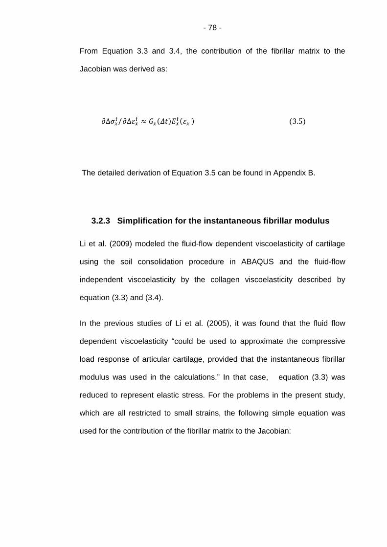
- 78 -
From Equation 3.3 and 3.4, the contribution of the fibrillar matrix to the
Jacobian was derived as:
Δߪ௫ Δߝ௫
/ ≈ ௫ܧ(ݐ߂)௫ܩ(ߝ௫ ) (3.5)
The detailed derivation of Equation 3.5 can be found in Appendix B.
3.2.3 Simplification for the instantaneous fibrillar modulus
Li et al. (2009) modeled the fluid-flow dependent viscoelasticity of cartilage
using the soil consolidation procedure in ABAQUS and the fluid-flow
independent viscoelasticity by the collagen viscoelasticity described by
equation (3.3) and (3.4).
In the previous studies of Li et al. (2005), it was found that the fluid flow
dependent viscoelasticity “could be used to approximate the compressive
load response of articular cartilage, provided that the instantaneous fibrillar
modulus was used in the calculations.” In that case, equation (3.3) was
reduced to represent elastic stress. For the problems in the present study,
which are all restricted to small strains, the following simple equation was
used for the contribution of the fibrillar matrix to the Jacobian:

- 79 -
௫ܧ௫(0)ܩ(ߝ௫ ) = ௫ܧ
+ ௫ܧகߝ௫ (3.6)
where ௫ܧ and ௫ܧ
க are constants independent of strain but dependent on
ݔ and (X, Y, Z). They were for the instantaneous modulus of the fibrillar
matrix, and thus were larger than those for the static equilibrium modulus. (Li
et al., 2009).
So for small deformation problems, the element ௫௫ܦ in the Jacobian matrix of
the fibril-reinforced model of cartilage was written as:
௫௫ܦ = +ߣ +ߤ2 ௫ܧ + ௫ܧ
கߝ௫ (3.7)
The subscript x in Formula 3.2 - 3.7 can be replaced with y or z to obtain the
corresponding equations in the ݕ or .directionݖ
3.2.4 Implementation in commercial FE software
In the numerical procedure of the user-defined material subroutine - ‘‘UMAT”
of Li et al. (2009), the equations derived above were implemented and
‘orthotropic properties were formulated with reference to the local Cartesian
coordinates at the element level’. This ‘‘UMAT” can modify the collagen fibril
modulus based on the fibrillar strain determined in the previous iterative step
of ABAQUS.
So the first step to use ‘‘UMAT” in the fibril-reinforced models is to define the
local Cartesian system for each element (or element set) using a separate

- 80 -
process. As the process is different for the 2D axisymmetric and 3D models,
the corresponding models are given in Sections 3.3 and 3.4 respectively.
3.3 Methods to Implement DT-MRI Data in the 2D Model
This section describes the method to define local coordinate system required
for the 2D fibril-reinforced axisymmetric model and the process to implement
the DT-MRI data. In addition, the steps to set up the 2D model are also
introduced.
3.3.1 Geometry and mesh of the 2D model
In the 2D axisymmetric FE model, only the right half of the modified DT-MRI
pixel grid of cartilage sample in Figure 2.1 was used as a structured mesh
(17 rows and 37 columns) with the aspect ratio = 1(Figure 3.1).
Figure 3.1horizo
ymm
etric
Axi
s
Z(2)
2D mesh corresponds to the pixel grid: (vertical axis: Z(2);ntal axis: X (1)).
S
X
(1)
- 81 -
3.3.2 Definition of the element level Cartesian coordinates inthe 2D model
The local x, y and z directions were defined for each element using the
‘‘Orientation’’ option in Abaqus (Li et al., 2009). The primary collagen
orientation (i.e. the principal eigenvector corresponding to the maximum
eigenvalue of the diffusion tensor; Section 2.2) was defined as the local x-
axis: the three components (Xij, Yij and Zij; i =1∙∙∙17, j=38∙∙∙74) of every
single principal eigenvector were implemented to the corresponding element
to represent the fibril orientation in this element.
The 3-points method (right hand rule) in Abaqus Analysis user’s manual
2.2.5 (Figure 3.2) was used to define the local coordinates system: ‘a’ is the
point lies on local x-axis and point ‘b’ is in the local x-y plane and near to
local y-axis. The local origin ‘c’ is defaulted to be coincide with the origin of
the global system and does not need to be input in ‘‘Orientation’’.
Figure 3.2 3-points method to define the local rectangular system (AbaqusAnalysis user’s manual Figure 2.2.5-1).
- 82 -
When a user-defined orientation is used with two-dimensional solid
axisymmetric elements, the direction must be redefined for the X'(x)- and
Z'(z)-axis: the third direction (hoop direction) must remain unchanged
(Abaqus Analysis user’s manual 2.2.5). So only the x- direction needs to be
defined, the z-direction will be confirmed automatically.
‘Distribution’ in ABAQUS was used to define local coordinate systems on an
element-by-element basis:
1) To define a DISTRIBUTION TABLE of “COORD3D, COORD3D”; then
define DISTRIBUTION for each element (or element set) referring to
the distribution table. The distribution table for the coordinates
specifies COORD3D twice to indicate that data for two three-
dimensional-coordinate points must be specified for each element in
the distribution.
2) To define ORIENTATION.
3) The ORIENTATION is then referred to by a general section definition.
As the hoop direction must remain unchanged, the three-dimensional
coordinates (bXk,bYk,bZk) of the second point for every single element
should be (0, 1, 0). Only the three components (Xij, Yij and Zij; i =1∙∙∙17, j =
38∙∙∙74) of every single principal eigenvector need to be implemented to the
first point of the corresponding element.
The detailed code to use “DISTRIBUTION” in ORIENTATION is modified
from Example 3 in Abaqus Analysis user’s manual 2.7.1 and displayed in
Figure 3.3:

- 83 -
*DISTRIBUTION TABLE, NAME=tab2COORD3D, COORD3D
*DISTRIBUTION, NAME=dist2, LOCATION=element, TABLE=tab2, aX0,aY0,aZ0,bX0,bY0,bZ0
element number, aX1,aY1,aZ1,bX1,bY1,bZ1element number, aX2,aY2,aZ2,bX2,bY2,bZ2
…
*ORIENTATION, NAME=ORI, DEFINITION=COORDINATESdist2
Figure 3.3 “Distribution” to define the local rectangular system for eachelement in 2D models (Abaqus Analysis user’s manual 2.7.1).
Using the ‘‘UMAT’’ option in Abaqus, the strain dependent Young’s modulus
derived in Section 3.2 was defined to the corresponding element of the 2D
axisymmetric model (Figure 3.4). These strains are available in output file of
Abaqus as the “elastic” strains (Figure 3.4; Abaqus User Subroutines
Reference Manual 1.1.36 UMAT User subroutine to define a material's
mechanical behavior).
After the implementation of ‘‘Orientation’’ and ‘‘UMAT’’, the 2D fibril-
reinforced model was set up (Figure 3.4).
*SOLID SECTION, ELSET=N_CART, material=CARTILAGE_MTL, ORIENTATION=ORI

- 84 -
Fi
3.
Th
pr
co
re
de
Th
wa
Th
ax
voxel grid2D mesh re
model
deYm‘UMAT’
strain
gure 3.4 Flowfibril-reinfo
4 Method
e method to
ocess to imp
ntrast to the
ctangular sys
fined.
3.4.1 Defi
the 3D m
e 3-points m
s also used.
e origin c, po
is in Figure 3
1. Local or
MRI
Modified DTI
Abaqus
Diffusion tensor
chart of to implementrced model.
to Implement DT-M
define local coordinat
lement the DT-MRI da
2D model, all of the
tem in the 3D fibril-re
nition of the element
odel
ethod in Abaqus Anal
int a lying on the local x
.5 were defined as below
igin c: coincide with glob
of cartilage
Principal eigenvector usedas primary collagen
D
e
t
t
in
l
ys
-
:
a
‘Orientation’ in Abaqus
T-MRI
RI Dat
system
a are d
hree c
forced
evel C
is use
axis an
.
l origin.
or
2D fibril-inforced
data and “UMAT”
a in the 3D mo
for the 3D mo
escribed in this
oordinate axes
model were req
artesian coord
r’s manual 2.2.5
d point b lying on
ientation
Strainpendentoung’sodulus
“elastic”
in the 2D
del
del and the
section. In
of the local
uired to be
inates in
(Figure3.2)
the local y-

- 85 -
2. Point a on local x-axis - terminal point of the principal eigenvector :
Similar to the way in the 2D model, i.e. (Xij, Yij and Zij; i =1∙∙∙17,
j=1∙∙∙74) is defined as the local x-axis (X' in Figure 3.2).
3. Point b on local y-axis - terminal point of vector ሬwhich is derived
below (Figure 3.4):
Vector :
Vector
and vector
=
Vecto
vector and
ሬ=
l
c
Figure 3.5 Definition of l
the unit vector (1, 0, 0) from
is the unit vector from origin
, defining the direction of lo
i.e. (0, -Zij, Yij) ……
r ሬ is the unit vector from
vector , defining the directi
i.e. (-Yij2-Zij
2, XijYij, X
ocal z-axis local y-axis ሬ
o
o
w
c
…
o
o
i
local x-axis
cal Y-axis (vector ሬ ).
rigin on global X-axis.
hich is the cross product of vector
al z-axis (Figure 3.5):
……… (3.8)
rigin which is the cross product of
n of local y-axis (Figure 3.5):
jZij) …………. (3.9)
global X-axis

- 86 -
3.4.2 Definition of the element level Cartesian coordinates in
the 3D model
To define the orientation of collagen fibril in each element set of the 3D
model, the code to use ‘Distribution’ is:
F
F
c
j
t
t
3
I
m
m
‘
*DISTRIBUTION TABLE, NAME=tab2COORD3D, COORD3D
*DISTRIBUTION, NAME=dist2, LOCATION=element, TABLE=tab2, aX0,aY0,aZ0,bX0,bY0,bZ0
element set number, aX1,aY1,aZ1,bX1,bY1,bZ1element set number, aX2,aY2,aZ2,bX2,bY2,bZ2
…
*ORIENTATION, NAME=ORI, DEFINITION=COORDINATESdist2
*SOLID SECTION, ELSET=N_CART, material=CARTILAGE_MTL, ORIENTATION=ORI
igure 3.6 ‘Distribution’ to define the local rectangular system for eachelement in 3D models (Abaqus Analysis user’s manual 2.7.1).
or the first coordinates point of the corresponding element set, the three
omponents of every single principal eigenvector (Xij, Yij and Zij; i =1∙∙∙17,
=1∙∙∙74) were directly implemented. But for the second coordinates point,
he three components were calculated in advance using Formula 3.9; then
he result of calculation was implemented to the corresponding element set.
.5 Summary
n order to set up the more realistic fibril reinforced poroelastic finite element
odels of articular cartilage incorporating the DT-MRI data, the material
odel employed in the analysis was developed first - the material subroutine
‘UMAT’’ in ABAQUS provided by Dr L. P. Li (University of Calgary) was

- 87 -
used to define the strain-dependent Young’s modulus of collagen fibril. The
detailed derivation of the equations used in the subroutine was provided in
the related literature.
The specific method to implement of the DT-MRI data in the 2D
axisymmetric and 3D model are described in Section 3.3 and Section 3.4
respectively. Meanwhile, the method to define the local y-axis in the 3D
model has been developed independently. Details are given of the input file
used to import the primary fibril orientation information.
These methods are adapted in the 2D and 3D fibril-reinforced models in
Chapter 4 and Chapter 5 respectively.

- 88 -
Chapter 4 Effect of Modelling Fibril Orientation in Two-
dimensional Axisymmetric Models
4.1 Introduction
Articular cartilage can be considered as a porous matrix saturated in water,
reinforced by a fibrillar network. The porous matrix is nonfibrillar,
representing the solid matrix excluding the collagen fibres as described in
Section 3.2. From the view of simulating the tissue structure, the constitutive
models of cartilage were classified as two types: the macroscopic models
without consideration of the underlying tissue structure and the
microstructural models mimicking the fibrillar network and the nonfibrillar
matrix separately (Taylor et al., 2006).
Different modeling studies on the anisotropic material properties of articular
cartilage: such as transversely isotropic models (Cohen et al., 1998 and
Soulhat et al., 1999) and fibril-reinforced models (Soulhat et al., 1999; Li et
al., 1999-2013; Wilson et al., 2004-2013; Shirazi et al., 2007 and Gupta
et.al., 2009). However, no direct comparative studies have been made
between the isotropic model and the fibril-reinforced model implementing
realistic fibril orientation.
The aim of the work presented in this chapter is to investigate the
capabilities of a 2D microstructural model (fibril-reinforced) in describing the
fluid load support. The basic modeling methodology, which incorporates the
material model described in Chapter 3, is introduced in the second section.
The 2D axisymmetric cases, of various levels of complexity, are given for

- 89 -
each case in terms of fluid load support, contact pressure, pore pressure
and fluid velocity.
A series of 2D axisymmetric models with poroelastic material were set up
systematically in the third section. First of all, a 2D isotropic poroelastic
model was created and the mesh sensitivity analysis was carried out in the
second section, in order to verify the rationality of the structured 2D mesh
modified from the DT-MRI pixel grid (Section 3.3). Then the verified mesh
was used in all of the 2D models in this section.
Then the results of the systematic models were compared and discussed in
the following two sections.
4.2 Model and Method
The collagen fibril orientations derived from the DT-MRI data (Chapter 2)
was implemented directly to the realistic fibril-reinforced model (Chapter 3).
The top 2 layers’ fibrils in Figure 2.2 were idealized to distribute horizontally
to set up the semi-realistic model, with the fibril orientations in the remaining
layers unchanged. Both of the above models employed strain dependent
Young’s modulus introduced in Section 3.2.2. The two uniform reinforced
models incorporated constant and strain dependent Young’s modulus
respectively, with the local coordination system defined same as the global
frame. The constant Young’s modulus in the isotropic and uniformly
reinforced models was adjusted, in order to let the vertical displacement in
the two models match the realistic fibril-reinforced model at the end of the
ramp loading.
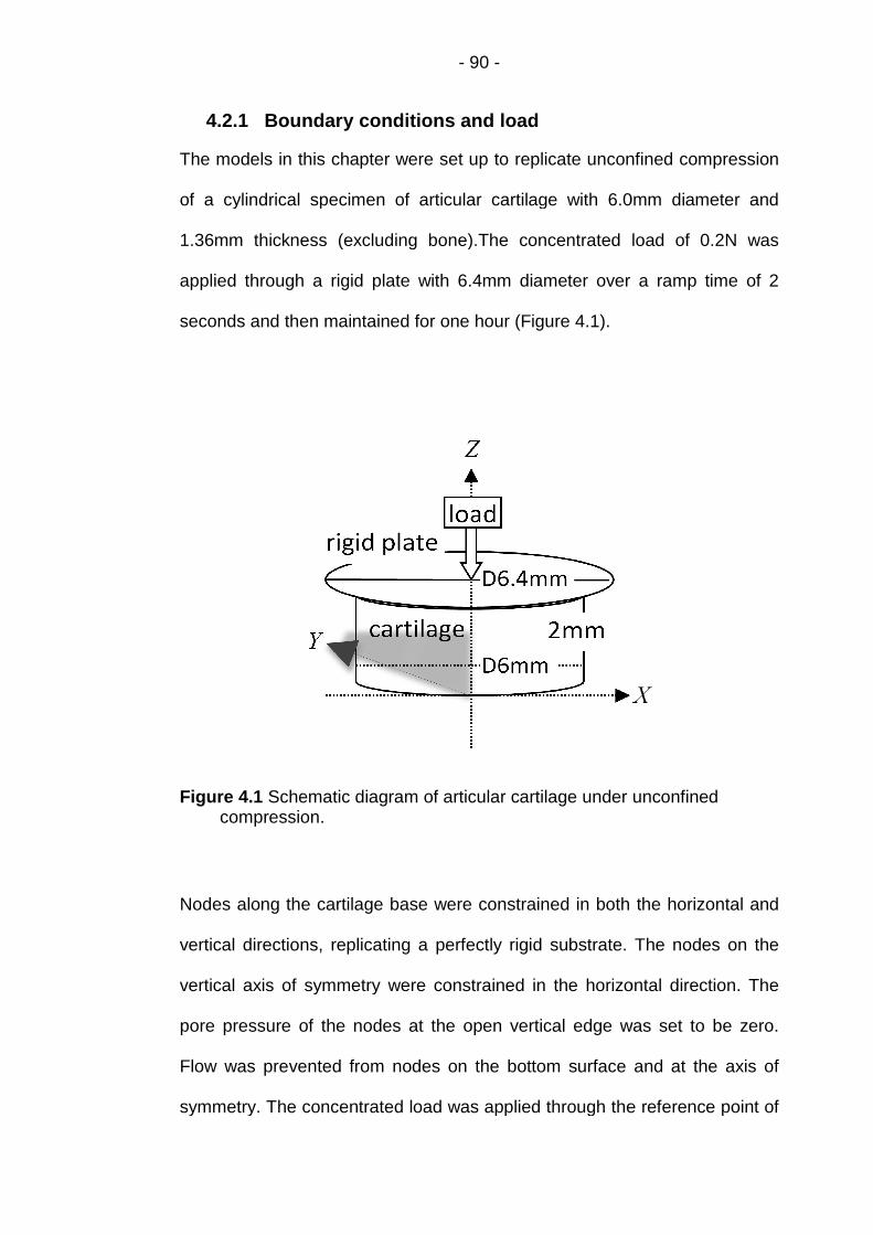
4.2.1 Boundary conditions and load
The models in this chapter were set up to replicate unconfined compression
of a cylindrical specimen of articular cartilage with 6.0mm diameter and
1.36mm thickness (excluding bone).The concentrated load of 0.2N was
applied through a rigid plate with 6.4mm diameter over a ramp time of 2
seconds and then maintained for one hour (Figure 4.1).
Figure 4.1 Schematic diagram of articular cartilage under unconfinedcompression.
Nodes along the cartilage
vertical directions, replicating a perfectly rigid substrate. The nodes on the
vertical axis of symmetry were constrained in the horizontal direction. The
pore pressure of the nodes at the open vertical edg
Flow was prevented from nodes on the bottom surface and at the axis of
symmetry. The concentrated load was applied through the reference point of
- 90 -
Boundary conditions and load
The models in this chapter were set up to replicate unconfined compression
of a cylindrical specimen of articular cartilage with 6.0mm diameter and
1.36mm thickness (excluding bone).The concentrated load of 0.2N was
ed through a rigid plate with 6.4mm diameter over a ramp time of 2
seconds and then maintained for one hour (Figure 4.1).
Schematic diagram of articular cartilage under unconfinedcompression.
Nodes along the cartilage base were constrained in both the horizontal and
vertical directions, replicating a perfectly rigid substrate. The nodes on the
vertical axis of symmetry were constrained in the horizontal direction. The
pore pressure of the nodes at the open vertical edge was set to be zero.
Flow was prevented from nodes on the bottom surface and at the axis of
symmetry. The concentrated load was applied through the reference point of
The models in this chapter were set up to replicate unconfined compression
of a cylindrical specimen of articular cartilage with 6.0mm diameter and
1.36mm thickness (excluding bone).The concentrated load of 0.2N was
ed through a rigid plate with 6.4mm diameter over a ramp time of 2
Schematic diagram of articular cartilage under unconfined
base were constrained in both the horizontal and
vertical directions, replicating a perfectly rigid substrate. The nodes on the
vertical axis of symmetry were constrained in the horizontal direction. The
e was set to be zero.
Flow was prevented from nodes on the bottom surface and at the axis of
symmetry. The concentrated load was applied through the reference point of

- 91 -
the rigid plate. The reference point was constrained in the horizontal
direction to prevent translating; its rotation was also constrained. A contact
condition, with a zero coefficient of friction, was created between the rigid
plate and the top surface of cartilage.
4.2.2 Element type and mesh
A two dimensional axisymmetric finite element model was created to
replicate the unconfined compression of cartilage (Figure 4.2). The mesh
used in this model had 629 elements (Figure 3.1), which is identical to a half
of the DT-MRI pixel grid: 17 rows and 37 columns with the aspect ratio = 1
(both horizontal and vertical resolutions are 70μm). The dimension of the
cartilage geometry in this model did not exactly match the sample in Figure
4.1 due to the limitation of the DT-MRI pixel grid: no diffusion tensor was
derived corresponding to the deepest part of cartilage (12.5% of the whole
cartilage thickness) since the low water content (Pierce et al., 2010); neither
in the side region of cartilage (13.7% of the cartilage radius) because of the
image noise.
The first-order bilinear pore pressure CAX4P was used in all of the two
dimensional models for the subsequent analyses in this chapter. First-order
elements were adopted for the slave surface, in the two dimensional contact
simulations, due to the possible problems created by the second-order
elements in calculating the “consistent nodal loads for constant pressure”
(ABAQUS Tutorials - Interactive Edition, 12.4.4). Furthermore, with the
bilinear pore pressure element, the aim to investigate the fluid pressure and
load support in cartilage could be readily investigated. However, hour-
glassing problem was caused when the reduced-integration elements

- 92 -
CAX4RP were used in the reinforced models implementing fibril orientation
and hence were not used.
Figure 4.2 Schematic diagram of the 2D axisymmetric FE model simulatingarticular cartilage under unconfined compression (vertical axis: Z;horizontal axis: X (r); into plane axis: Y (θ)).
4.2.3 Material model
Each of the model cases created were assigned a poroelastic material
property, where both a solid and fluid phase were considered. In cases
where fibre reinforcement was included a distribution of fibre orientations
was created. The material model was modified in these local fibre
directions. Where needed, fibril strain-dependence was introduced using a
user-defined material subroutine. Details of this method are given in
Chapter 3.

- 93 -
4.2.4 Mesh sensitivity analysis of the 2D isotropic model
In order to analyze the mesh sensitivity on the peak value of fluid load
support, poroelastic material was employed in the 2D axisymmetric isotropic
FE model:
For the solid elastic matrix, the material parameters were the Young’s
modulus E (Mononen et al., 2010) and the Poisson’s ratio ν (Li et al., 2009).
The fluid flow within the matrix was described by the permeability k and the
initial void ratio e0 (pore volume over solid volume; Li et al., 1999 and 2009),
which is required in the input file of ABAQUS. All material parameters were
constant through the tissue depth (Table 4.1) i.e. the model was
homogenous.
Table 4.1 Material parameters of isotropic model.
Material parameter Value
Young’s modulus, E 0.69 MPa
Poisson’s ratio, v 0.36
Permeability, k 3.0 x 10⁻¹⁵ m4/N∙s
Initial void ratio, e0 4.0(80% interstitial fluid)
Mesh sensitivity analysis was carried out by reducing the element number by
a factor of roughly 1/4 (1/2 × 1/2) and increasing it twice by 2 × 2 times. The
coarser mesh had 144 (8 × 18) elements; the denser meshes had 2516 (34
× 74) and 10064 (68 × 148) elements respectively.

- 94 -
After 2 second of ramp deformation, the contact pressure distributions on
cartilage surface did not show significant differences in most of the contact
zone (Figure 4.3), except on the area near the open side (right edge in
Figure 3.1) where the curve of 8 × 18 elements being slightly outside than
those of other mesh densities. However, the curve of 17 × 37 elements used
in the 2D isotropic model was much closer to both of the densest ones which
nearly coincided to each other.
Figure 4.3 Distribution of contact pressure on cartilage surface at the end oframp load (t = 2s).
As for the pore pressure, the curves of the two coarser meshes with 8 × 18
and of 17 × 37 elements both matched the two densest ones on the whole
cartilage surface (Figure 4.4).
0
2
4
6
8
10
12
14
16
0 0.5 1 1.5 2 2.5 3
Co
nta
ctP
ress
ure
(KP
a)
Radial Distance from Symmetric Axis (mm)
8x18
17x37
34x74
68x148
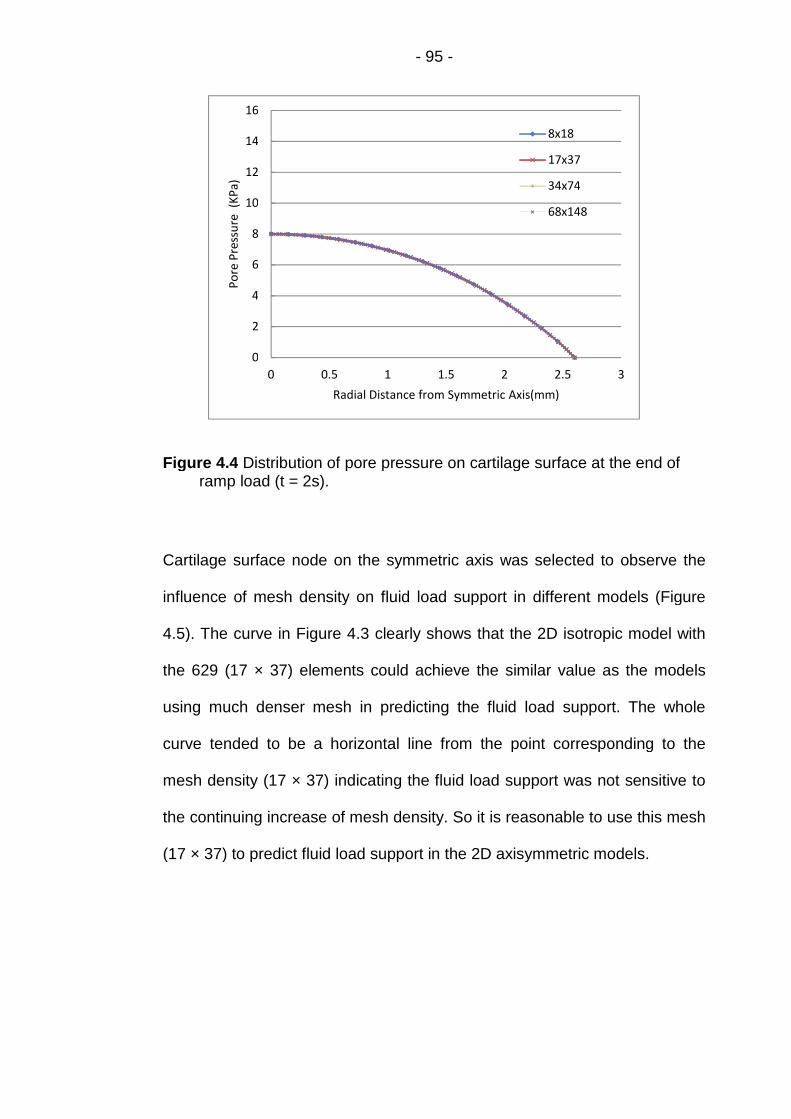
- 95 -
Figure 4.4 Distribution of pore pressure on cartilage surface at the end oframp load (t = 2s).
Cartilage surface node on the symmetric axis was selected to observe the
influence of mesh density on fluid load support in different models (Figure
4.5). The curve in Figure 4.3 clearly shows that the 2D isotropic model with
the 629 (17 × 37) elements could achieve the similar value as the models
using much denser mesh in predicting the fluid load support. The whole
curve tended to be a horizontal line from the point corresponding to the
mesh density (17 × 37) indicating the fluid load support was not sensitive to
the continuing increase of mesh density. So it is reasonable to use this mesh
(17 × 37) to predict fluid load support in the 2D axisymmetric models.
0
2
4
6
8
10
12
14
16
0 0.5 1 1.5 2 2.5 3
Po
reP
ress
ure
(KP
a)
Radial Distance from Symmetric Axis(mm)
8x18
17x37
34x74
68x148

- 96 -
Figure 4.5 Fluid load support at cartilage surface node on the symmetry axisof different mesh density at the end of ramp load (t = 2s).
4.2.5 Parameter predictions of 2D models
Theoretically, the peak value of pore pressure should occur at the end of the
ramp time. So most of the results used in the analysis are at the moment of t
= 2s. The parameters of 2D models displayed below are measured in this
chapter:
Contact pressure, pore pressure and fluid load support on cartilage
surface
The total pressure on the contact area of cartilage surface may be different
as the tissue particularly the collage fibril distribution is anisotropic. Wear
and tear of cartilage may be related to the contact pressure, so it is crucial to
investigate the contact pressure on the surface. Meanwhile, the pore
pressure along the cartilage surface plays a vital role in the of tribology study
within the human knee joint according the theory of biphasic lubrication. So it
50
52
54
56
58
60
0 2000 4000 6000 8000 10000 12000
Flu
idLo
adSu
pp
ort
(%)
Number of Elements Used in Different models

- 97 -
is important to record and compare the peak values of contact pressure and
pore pressure on the surface of cartilage.
In the biphasic lubrication theory, fluid load support - the ration of contact
pressure and pore pressure is more important than each individual variable.
It represents the amount of applied load carried by the liquid phase in the
cartilage. The most important thing is that it can interpret tribological
mechanism of the load carrying between the solid and the liquid phase in the
tissue and hence directly influence the friction coefficients on the cartilage
surface.
The fluid velocity and contour of pore pressure
The fluid velocity (FLVEL) inside the cartilage represents the direction and
magnitude of the fluid flow within the tissue, while the FLVEL on the open
edge (open side) shows the speed of the interstitial fluid flowing out. The
differences of pore pressure at the various parts of cartilage, illustrated by
the contour, make the interstitial fluid flowing from the parts where pore
pressure is higher to the other parts with lower pore pressure.
The radial and axial deformation of cartilage open edge
The pore pressure is a result of the interstitial fluid pressurization. In order to
investigate the influence of collagen fibril implementation on the
pressurization, the radial and axial deformation of cartilage open edge in
different models were also recorded and compared to each other.
The radial stress on the cartilage surface

- 98 -
For the pathological investigation of the influence of collagen fibril
implementation, the radial stress on the cartilage surface in all of the five 2D
models was compared.
4.3 Modelling Cases
Three groups of 2D axisymmetric models were set up with different material
settings: the realistic fibril orientation model and the simplified fibril
orientation model (top 2 layers’ fibril were designed to distribute horizontally)
with strain dependent fibrillar Young’s modulus (named DT-MRI and DT-
MRI-top model respectively); the Uniform reinforced models with constant
fibrillar Young’s modulus (Uniform-Cons model) and the strain dependent
fibrillar Young’s modulus (Uniform-SD model); and the basic model with
isotropic poroelastic material (Isotropic model) - totally five modelling cases.
The geometry, mesh, boundary conditions and loading in Figure 4.2 were
used in all of the five models. The material properties employed in these
models, including the collagen fibril orientation (except in the Isotropic
model), are described in Table 4.2.

- 99 -
Table 4.2 Material properties of different models (ε is the fibrillar strain ineach iteration and initial void ratio 4.0 represented 80% interstitial fluid).
Modelling
case
Material
parameter
DT-MRI based group Uniformly reinforced
group
DT-MRIDT-MRI-
top
Uniform-
SD
Uniform-
ConsIsotropic
Young’s
modulus of
nonfibrillar
matrix, Em
(MPa)
0.26 0.26 0.26 0.26 0.91
Poisson’s ratio
of nonfibrillar
matrix, vm
0.36 0.36 0.36 0.36 0.36
Young’s
modulus of
fibril, Efx and
Efy (MPa)
3+1600ε 3+1600ε 3+1600ε 2.15 n/a
Permeability, k
(m4/N∙s)3.0 × 10-15 3.0 × 10⁻¹⁵ 3.0 ×10⁻¹⁵ 3.0 ×10⁻¹⁵ 3.0 ×10⁻¹⁵
Initial void
ratio, e0
4.0 4.0 4.0 4.0 4.0
Orientation
source for top
2 layers
DT-MRIManual
uniform
Manual
uniform
Manual
uniformn/a
Orientation
source for
lower 15
layers
DT-MRI DT-MRIManual
uniform
Manual
uniformn/a

- 100 -
The deformation of cartilage in different models under the same load would
be dissimilar due to the completely different properties of material, although
all other modelling factors were same. This made it difficult to compare the
modelling results, since the cartilage deformation and fluid load support are
closely related. In order to make the comparison reasonable, the value of
Young’s modulus in both the local x and y directions in Cons E model should
be adjusted to match the vertical displacement of the cartilage surface in the
DT-MRI model at the end of the ramp loading stage. The similar adjustment
was done in the Isotropic model. To provide the information of the cartilage
deformation to carry out this adjustment, the DT-MRI model was set up first.
4.3.1 Models of the DT-MRI based group
4.3.1.1 Mechanical property of material
In both of the DT-MRI and DT-MRI-top models, the nonfibrillar poroelastic
matrix was isotropic with the Young’s modulus Em = 0.26 MPa, Poisson’s
ratio mߥ = 0.36, permeability k = 0.003 mm4/Ns and the initial void ratio e0 =
4.0 (Li et al., 1999 and 2009). The Young’s modulus of the fibrillar network
was designed to be the same in the local x and y directions, Efx = Efy = 3 +
1600ε MPa (Efx and Efy represents modulus in local x and y direction
respectively), where ε is the fibrillar strain (Li et al., 2009) as described in
Chapter 3; while the Young’s modulus in the local z directions Efz = 0 MPa.
The values of the material parameters are displayed in Table 4.2.
The strain dependent Young’s modulus of the fibrillar network (3 + 1600ε
MPa) was implemented using the user-defined subroutine “UMAT” in
ABAQUS provided by Dr L. P. Li, University of Calgary.

- 101 -
4.3.1.2 Implementation of fibril orientation
The user-defined “ORIENTATION” including “Distribution” introduced in
Section 3.3 was used to incorporate the fibril orientation in each of the 2D
solid axisymmetric elements: the principal eigenvector of a specific diffusion
tensor was defined as the x-axis of the local Cartesian coordinates of the
corresponding element.
ABAQUS requires the direction must be redefined for the local x- and z-axis
while the local y-axis must remain identical with the global hoop direction
(Abaqus Analysis user’s manual 2.2.5). So only the direction of the local x-
axis needed to be defined, the local z-axis would be confirmed automatically
by right-hand rule in ABAQUS.
“ORIENTATION” in the DT-MRI model
The realistic fibril orientations derived from DT-MRI were incorporated in the
DT-MRI model: the three components (Xij, Yij and Zij; i =1∙∙∙17, j=38∙∙∙74) of
every single principal eigenvector were implemented to the corresponding
element in Figure 3.2 to represent the fibril orientation in this element. As the
element number in Figure 3.2 was increasing from bottom to top, the three
components of principal eigenvector for the first element should be (X17,38,
Y17,38 , Z17,38); part of the detailed code corresponding to Figure 3.3 is
displayed below:

- 102 -
In
d
e
e
c
c
*DISTRIBUTION TABLE, NAME=tab2
COORD3D, COORD3D
*DISTRIBUTION, NAME=dist2, LOCATION=element, TABLE=tab2
, aX0,aY0,aZ0,bX0,bY0,bZ0
1, X17,38,Y17,38,Z17,38,0,1,0
2, X17,39,Y17,39,Z17,39,0,1,0
…
37, X17,74,Y17,74,Z17,74,0,1,0
38, X16,38,Y16,38,Z16,38,0,1,0
…
74, X16,74,Y16,74,Z16,74,0,1,0
…
629, X1,74,Y1,74,Z1,74,0,1,0
*ORIENTATION, NAME=ORI, DEFINITION=COORDINATES, SYSTEM=RECTANGULAR
dist2
“ORIENTATION” in the DT-MRI-top model
this model, fibrils in the top 2 layers in Figure 3.2 were designed to
istribute horizontally. So the three components of every single principal
igenvector in the corresponding element (from the 556th to the 629th
lement) in the top 2 layers was (1,0,0), while the local Cartesian
oordinates in others elements did not changed. The subroutine was
hanged as:
*SOLID SECTION, ELSET=N_CART, material=CARTILAGE_MTL, ORIENTATION=ORI

- 103 -
B
s
fi
d
m
Y
a
th
C
In
U
*DISTRIBUTION TABLE, NAME=tab2
COORD3D, COORD3D
*DISTRIBUTION, NAME=dist2, LOCATION=element, TABLE=tab2
, aX0,aY0,aZ0,bX0,bY0,bZ0
1, X17,38,Y17,38,Z17,38,0,1,0
2, X17,39,Y17,39,Z17,39,0,1,0
…
555, X3,74,Y3,74,Z3,74,0,1,0
556, 1,0,0,0,1,0
…
629, 1,0,0,0,1,0
*ORIENTATION, NAME=ORI, DEFINITION=COORDINATES, SYSTEM=RECTANGULAR
dist2
4.3.2 Models of the uniform reinforced group
oth of the Uniform-Cons model and the Uniform-SD model were the further
implification of the DT-MRI-top model: no specific orientation of collagen
brils were implemented, the local Cartesian coordinate in each element was
efined to be the same as the global system. The two uniform reinforced
odels were set up to investigate the influence of the strain dependent
oung’s modulus of the fibrillar network by comparing to each other, and
lso the effect of fibril orientation implementation through the contrast with
e DT-MRI model.
4.3.2.1 Mechanical property of material
Uniform reinforced model with constant Young’s modulus (Uniform-
ons)
order to make the vertical deformation of the cartilage surface of the
niform reinforced models match the DT-MRI model at the end of the ramp
*SOLID SECTION, ELSET=N_CART, material=CARTILAGE_MTL, ORIENTATION=ORI

- 104 -
loading stage, the value of the Young’s modulus Efx and Efy (represents
modulus in local x and y direction respectively) in this model was adjusted
while Efz = 0 (Figure 4.6).
In Figure 4.6, only the curve of the Uniform-Cons model with 2.15MPa
Young’s modulus could match the vertical deformation of the cartilage
surface of the DT- MRI model at t = 2s. The other material parameters in this
model (Table 4.3) were the same as the DT- MRI model. The user-defined
subroutine “UMAT” was still used in this model, although the Young’s
modulus was constant.
Figure 4.6 Adjustments of Young’s modulus in the Cons E model to achievethe same maximum axial displacement as DT-MRI model at the end oframp loading (t = 2s).
Uniform reinforced model with strain dependent Young’s modulus
(Uniform-SD)
0
0.1
0.2
0.3
0.4
0.5
0.6
0.7
0.8
0 0.5 1 1.5 2
Rel
ativ
ely
Axi
alD
efo
rmat
ion
(%)
Ramp Loading Time (s)
DT-MRI
Uniform-Cons E2.15
Uniform-Cons E1.8
Uniform-Cons E2.0
Uniform-Cons E2.2

- 105 -
The mechanical property parameters and their values of cartilage in this
model were same as the DT-MRI model (Table 4.2) i.e. the Young’s
modulus Efx and Efy was (3 + 1600ε MPa) respectively while Efz = 0. The
user-defined subroutine “UMAT” was also used in this model to implement
the strain dependent Young’s modulus of the fibrillar network.
4.3.2.2 Definition of the local coordinate system
For each element, the local Cartesian system was aligned with the global
system. This effectively aligned the fibril orientation with the global X-axis in
each case. Therefore, when the material model was modified based on this
orientation, each element was given an equal, maximum reinforcement in
the local x-direction. Instead of the user-defined “ORIENTATION” including
“Distribution” in Section 3.3, the ‘Keyword’ method was used to define the
local system by specifying the locations of points a, b, and c directly (Abaqus
Analysis User's Manual 2.2.5). The data lines to define the orientation using
DEFINITION=COORDINATES can be found in “ORIENTATION” of Abaqus
Keywords Reference Manual. The detailed input file in these two models to
define the local Cartesian coordinate was:
I
i
*Orientation, name=Ori-1, DEFINITION=COORDINATES, SYSTEM=RECTANGULAR
1.0, 0.0, 0.0, 0.0, 1.0, 0.0
4.3.3 The isotropic poroelastic model
n order to produce the comparable results, the value of Young’s modulus E
n Table 1 was adjusted to be 0.91MPa to make the vertical deformation of

- 106 -
the cartilage surface in Isotropic model match the DT- MRI model at the end
of the ramp loading stage (Figure 4.7).
Figure 4.7 Adjustments of Young’s modulus in the ISO model to achieve thesame maximum axial displacement as DT- MRI model at the end oframp loading (t = 2s).
4.4 Results
The results from different models such as the contact pressure, the pore
pressure, the fluid load support and the stress along the cartilage surface
were collected and compared in a same figure. The axial and radial
displacements of nodes on the open side were also compared. The fluid
velocity and the contour of pore pressure through the whole cartilage sample
were displayed separately.
0
0.1
0.2
0.3
0.4
0.5
0.6
0.7
0.8
0 0.5 1 1.5 2
Rel
ativ
ely
Axi
alD
efo
rmat
ion
(%)
Ramp Loading Time (s)
DT-MRI
Isotopic-E0.69
Isotropic-E0.93
Isotropic-E0.91

- 107 -
In all of the modelling cases, nodes at the bottom of the lowest layer were
prevented from displacing by the applied boundary conditions at that point;
the radial deformation was normalized by the cartilage radius (2.59 mm) and
the axial deformation by the cartilage thickness (1.19 mm).
4.4.1 Contact pressure, pore pressure and fluid load support
on cartilage surface
Variation of the contact pressure distribution along the cartilage surface was
apparently different among the three model-groups (Figure 4.8): The DT-
MRI and DT-MRI-top model had a much higher maximum value but
decreased faster while the other models varied smoothly. The slight
difference between the curves of Uniform-Cons and Uniform-SD models
showed that the strain dependent Young’s modulus of collagen fibril did not
affect contact pressure markedly in this group.
Figure 4.8 Distribution of contact pressure along cartilage surface at the endof ramp loading (t = 2s).
0
10
20
30
40
50
60
0 0.5 1 1.5 2 2.5 3
Co
nta
ctP
ress
ure
(kP
a)
Radial Distance from Symmetric Axis (mm)
Isotropic
Uniform-Cons
Uniform-SD
DT-MRI
DT-MRI-top

- 108 -
Figure 4.9 clearly shows that fibril reinforcement could increase the value of
pore pressure comparing to the ISO model. It can also be found that strain
dependent Young’s modulus influenced pore pressure of Uniform-SD model
more apparently than it did on contact pressure in Figure 4.8.
Figure 4.9 Distribution of pore pressure along cartilage surface at the endof ramp loading (t = 2s).
The value of fluid load support at the contact zone of cartilage surface in the
four models with fibril reinforcement increased markedly compared to the
simple Isotropic model (from <60% to >80%), although there were more
fluctuations in the curve of the DT-MRI model than those of the other three
models (Figure 4.10).
0
10
20
30
40
50
60
0 0.5 1 1.5 2 2.5 3
Po
reP
ress
ure
(kP
a)
Radial Distance from Symmetric Axis (mm)
Isotropic
Uniform-Cons
Uniform-SD
DT-MRI
DT-MRI-top

- 109 -
Figure 4.10 Comparison of fluid load support along cartilage surface at theend of ramp loading (t = 2s).
Figures 4.8 - 4.10 clearly show the peak value of observed parameters
located on the symmetric centre of cartilage surface (except the fluid support
of DT-MRI and DT-MRI-top models). The detailed values of the observed
parameters at the end of ramp loading (t = 2s) are compared in Table 4.4.
0
10
20
30
40
50
60
70
80
90
100
0 0.5 1 1.5 2 2.5 3
Flu
idLo
adSu
pp
ort
(%)
Radial Distance from Symmetric Axis
Isotropic
Uniform-Cons
Uniform-SD
DT-MRI
DT-MRI- top

- 110 -
Table 4.4 Comparison of results on axisymmetric surface centre of cartilagesample at the end of ramp loading (t = 2s).
Although the peak value of fluid load support in the Uniform-SD model was
similar as that of the DT-MRI model (Table 4.4), it decreased much more
rapidly after ramp load, while the load was maintained (Figure 4.11).
Results on surface
centre
Models
Contact
pressure
( KPa)
Pore
pressure
( KPa)
Fluid loadsupport
(%)
Isotropic model 14.15 8.18 57.80
Uniformreinforced
models
Uniform-Cons 11.67 11.0 87.33
Uniform-SD 11.91 11.10 93.26
Realisticfibril
distributionmodels
DT-MRI 52.26 50.06 95.78
DT-MRI-top 50.95 47.57 93.35

- 111 -
Figure 4.11 Comparison of fluid load support at the centre of cartilagesurface during loading period.
4.4.2 The fluid velocity of cartilage
The fluid velocity (FLVEL) was fairly homogeneous in the Isotropic model
and the Uniform reinforced models (Figure 4.12). In those cases, it
increased from top to bottom along the open side (right) edge of cartilage
although the magnitude was obviously higher in the two latter models. Both
uniformly reinforced models generated velocity maps which were aligned
with the fibril orientation, showing less fluid movement between layers than
in the isotropic case.
0
10
20
30
40
50
60
70
80
90
100
0 800 1600 2400 3200 4000
Flu
idLo
adSu
pp
ort
atC
arti
lage
Surf
ace
Ce
ntr
e(%
)
Loading Time (s)
Isotropic
Uniform-ConsUniform-SD
DT-MRI

- 112 -
(a)
(b)
(c)
(d)
(e)
Figure 4.12 Fluid velocity (mm/s) of (a) Isotropic, (b) Uniform-Cons, (c)Uniform-SD, (d) DT-MRI and (e) DT-MRI-top at the end of ramp loading(t = 2s).
- 113 -
In the DT-MRI and DT-MRI-top cases, the velocity direction was highly
variable. The higher velocity magnitude close to the Isotropic model and the
Uniform reinforced models but much more concentrated around the
symmetric axis. The lower magnitude close to the open edge implies that the
fluid was trapped and less had been expelled at this time point (t = 2s). In
the meantime, no apparent difference was found between the two models in
the same group, except the more regular distribution in the first layer
elements of the DT-MRI-top model compared to the DT-MRI model (Figure
4.12).
4.4.3 The contour of pore pressure within cartilage
The map of pore pressure throughout the tissue was similar for the two
models within the same group. This is particularly clear for the two DT-MRI
based models (Figure 4.13). However, the contours of pore pressure
showed apparent differences in magnitude and distribution among the three
groups of models. Low pressure region near the open edge is much wider in
the DT-MRI group models than in the Uniform reinforced models; it is even
wider near the cartilage surface in the Isotropic model but decreases rapidly
to the cartilage bottom. High pressure regions near the symmetric axis in the
DT-MRI group models confirm that fluid is trapped and pressurised in that
area, when compared to the uniform distribution in the other cases (Figure
4.13).

- 114 -
(a)
(b)
(c)
(d)
(e)
Figure 4.13 Contour of pore pressure (MPa) of (a) Isotropic, (b) Uniform-Cons, (c) Uniform-SD, (d) DT-MRI and (e) DT-MRI-top model at theend of ramp loading (t = 2s).
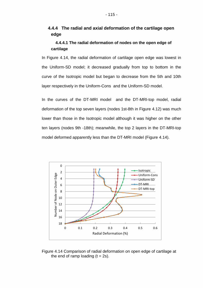
- 115 -
4.4.4 The radial and axial deformation of the cartilage open
edge
4.4.4.1 The radial deformation of nodes on the open edge of
cartilage
In Figure 4.14, the radial deformation of cartilage open edge was lowest in
the Uniform-SD model; it decreased gradually from top to bottom in the
curve of the Isotropic model but began to decrease from the 5th and 10th
layer respectively in the Uniform-Cons and the Uniform-SD model.
In the curves of the DT-MRI model and the DT-MRI-top model, radial
deformation of the top seven layers (nodes 1st-8th in Figure 4.12) was much
lower than those in the Isotropic model although it was higher on the other
ten layers (nodes 9th -18th); meanwhile, the top 2 layers in the DT-MRI-top
model deformed apparently less than the DT-MRI model (Figure 4.14).
Figure 4.14 Comparison of radial deformation on open edge of cartilage atthe end of ramp loading (t = 2s).
0
2
4
6
8
10
12
14
16
18
0 0.1 0.2 0.3 0.4 0.5 0.6
Nu
mb
ero
fN
od
eo
nO
ute
rEd
ge
Radial Deformation (%)
Isotropic
Uniform-Cons
Uniform-SD
DT-MRI
DT-MRI-top

- 116 -
4.4.4.2 The axial deformation of the cartilage open edge
Although the Isotropic and Uniform-Cons model was designed to match the
axial deformation of the DT-MRI model at the end of ramp loading (Figure
4.6 and 4.7), the axial displacement of each individual node along the open
edge and the axial deformation of each layer of cartilage may be different.
The axial displacement of each node along the open edge of cartilage
The axial displacements of the nodes on the open edge of cartilage in the
three models with same total axial deformation (i.e. Isotropic, Uniform-Cons
and DT-MRI) were truly different. But between the corresponding nodes in
the two models of DT-MRI group, only on the upper parts of the open
cartilage edges were slight difference found while the lower parts of the open
edges were nearly coincide. Nodes in the Uniform-SD model had the lowest
axial displacements compared to the other four models (Figure 4.15).
Figure 4.15 Comparison of axial displacement of nodes along the open edgeof cartilage at the end of ramp loading (t = 2s).
0
2
4
6
8
10
12
14
16
18
0 0.1 0.2 0.3 0.4 0.5 0.6
Nu
mb
ero
fN
od
eo
nR
igh
tEd
ge
Axial Deformation (%)
Isotropic
Uniform-Cons
Uniform-SD
DT-MRI
DT-MRI-top

- 117 -
The axial deformation of each layer of the cartilage
The axial deformation of a specific cartilage layer was defined as the
difference of the axial displacement of the top and bottom vertex of the
corresponding element along the open edge. This can be calculated from
Figure 4.15: the difference of two contiguous nodes in the same curve (from
top to bottom) was the axial deformation of cartilage layer between the two
nodes (Figure 4.16). As the curves of the two models of DT-MRI group are
nearly coincide (Figure 4.15), the axial deformation of cartilage layers of the
DT-MRI-top model was not calculated in order to make the curves more
distinguishable.
Figure 4.16 Comparison of axial deformation of elements along the openedge of cartilage at the end of ramp loading (t = 2s).
0
2
4
6
8
10
12
14
16
18
-0.05 0 0.05 0.1 0.15 0.2
Nu
mb
ero
fLa
yer
(To
pto
Bo
tto
m)
Normalized Deformation of Each Layer (%)
Isotropic
Uniform-Cons
Uniform-SD
DT-MRI-SD

- 118 -
4.4.5 The radial stress on the cartilage surface
Radial stress around the symmetric axis along the cartilage surface was
much higher in the two groups of fibril reinforced models than that in the
Isotropic model. Larger fluctuations appeared in the curve of the DT- MRI
model compared to the DT-MRI-top model, while the curves of other three
models distributed smoothly (Figure 4.17).
Figure 4.17 Distribution of radial stress (S11) along cartilage surface at theend of ramp loading (t = 2s).
4.4.6 The axial deformation of cartilage during loading period
The normalized axial deformation of cartilage was compared across all five
models during the full loading period (Figure 4.18). After one hour’s creep all
models had reached equilibrium with the exception of the group of DT-MRI
based models.
0
5
10
15
20
25
30
35
0 0.5 1 1.5 2 2.5 3
Rad
ial
Sre
ss(k
Pa)
Radial Distance from Symmetric Axial (mm)
Isotropic
UniformCons
Uniform-SD
DT-MRI
DT-MRI-top
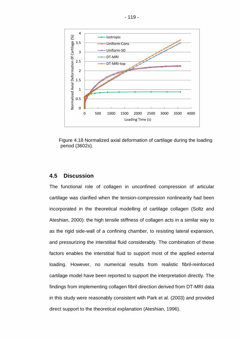
- 119 -
Figure 4.18 Normalized axial deformation of cartilage during the loadingperiod (3602s).
4.5 Discussion
The functional role of collagen in unconfined compression of articular
cartilage was clarified when the tension-compression nonlinearity had been
incorporated in the theoretical modelling of cartilage collagen (Soltz and
Ateshian, 2000): the high tensile stiffness of collagen acts in a similar way to
as the rigid side-wall of a confining chamber, to resisting lateral expansion,
and pressurizing the interstitial fluid considerably. The combination of these
factors enables the interstitial fluid to support most of the applied external
loading. However, no numerical results from realistic fibril-reinforced
cartilage model have been reported to support the interpretation directly. The
findings from implementing collagen fibril direction derived from DT-MRI data
in this study were reasonably consistent with Park et al. (2003) and provided
direct support to the theoretical explanation (Ateshian, 1996).
0
0.5
1
1.5
2
2.5
3
3.5
4
0 500 1000 1500 2000 2500 3000 3500 4000
No
rmal
ized
Axi
alD
efo
rmat
ion
0f
Car
tila
ge(%
)
Loading Time (s)
Isotropic
Uniform-Cons
Uniform-SD
DT-MRI
DT-MRI-top

- 120 -
4.5.1 The effect of the user defined subroutine “UMAT”
4.5.1.1 The effect on the surface zone of cartilage
With the implementation of “UMAT” to the four reinforced models, the
Young’s modulus in the axial direction (0.26 MPa) was defined much lower
than in the Isotropic model (0.91 MPa). Theoretically, the axial deformation
of the upper part of cartilage (the top two layers in Figure 4.2) in the
reinforced models would be much greater than in the Isotropic model.
However, the axial deformation of the top two cartilage layers in the
reinforced models was nearly same as in the Isotropic model except slightly
larger in the Uniform-Cons model (Figure 4.16). This was due to the
powerful reinforcement of the large Young’s modulus in the radial direction
((0.26 + 2.15) MPa in the Uniform-Cons model or (0.26 + 3 +1600ε) MPa in
the other three models) defined by the “UMAT”.
Compared to the Isotropic model, the cartilage surface in these four models
was strengthened in the radial direction and became tangentially stiffer -
radial stress around the symmetric axis along cartilage surface was
therefore much higher in these models than that in the Isotropic model
(Figure 4.17). Similarly, the underneath part of the top two layers of cartilage
was also somewhat strengthened and became tangentially stiffer. When the
cartilage was compressed, this upper zone in the reinforced models moved
down readily with less radial deformation than those in Isotropic model
(Figure 4.14) i.e. the lateral expansion of this zone was resisted by the
higher tensile stiffness of collagen fibril in the reinforced models. Hence,
pressurization of interstitial fluid in the upper part of cartilage in the
reinforced models was enhanced markedly and higher pore pressure was

- 121 -
produced (Figure 4.9 and Table 4.4) to support the applied load (Figure
4.10).
4.5.1.2 The effect on pore pressure and fluid velocity throughout
the cartilage
As the hop direction remained unchanged in the 2D axisymmetric models,
the Young’s modulus in this direction was still much greater than in the axial
direction in the deeper region under the top two layers of cartilage in the
reinforced models. So the “UMAT” not only enhanced the pressurization of
interstitial fluid in the upper part of cartilage (Figure 4.9), but also throughout
the tissue to produce different fluid flow in contrast with the Isotropic model
(Figure 4.12 and 4.13).
As mentioned in Section 4.2.5, the differences of pore pressure at the
various parts of cartilage made the interstitial fluid flowing from the parts with
higher pore pressure to the other parts where pore pressure was lower. In
the uniformly reinforced models implementing “UMAT”, high pore pressure
distributed in the majority area of cartilage ((b) and (c) in Figure 4.13)
leading to the fairly homogeneous fluid velocity within the tissue ((b) and (c)
in Figure 4.12). Meanwhile, zero pore pressure distributed along the outer
edge almost evenly and the adjacent area with low pore pressure was
narrow ((b) and (c) in Figure 4.13). The higher pore pressure next to these
two area produced a high fluid velocity and let the interstitial fluid flowed
freely out through the whole edge ((b) and (c) in Figure 4.12).
For the Isotropic model, zero pore pressure distributed more and more wide
from bottom to top along the outer cartilage edge ((a) in Figure 4.13). So the
large difference of pore pressure was only produced near the corner

- 122 -
between the outer edge and the bottom of cartilage ((a) in Figure 4.13)
leading to the concentrated high fluid velocity at this corner ((a) in Figure
4.12).
4.5.2 The influence of the realistic fibril orientation
In the DT-MRI group models, the implementation of the realistic fibril
orientation caused an inhomogeneous pore pressure field ((d) and (e) in
Figure 4.13). The fluid was channelled towards lower pressure elements
causing bottlenecks in the flow. It therefore took more time for the fluid to be
expelled from the structure and a larger amount of pressure was built for a
particular ramp load. Furthermore, the area of zero pore pressure and the
adjacent low pressure area ((d) and (e) in Figure 4.13) were much wider
than those in the uniformly reinforced models ((b) and (c) in Figure 4.13).
The fluid in these two area could not get the high velocity from the tiny
pressure difference between the two area. So the fluid flowing out of the
cartilage was much less than in the uniformly reinforced models ((d) and (e)
in Figure 4.12). All of these factors caused by the realistic fibril orientation
combined together and led to the long maintaining of the high fluid load
support at the centre of cartilage surface (Figure 4.11) although this is not
consistent with the literature (Mow et al., 2005). However, this phenomena
was also found in the equilibrium model of Kazemi et al. (2011) using the
same “UMAT” and also implementing the realistic fibril orientation: the value
of pore pressure was also remarkably high (66% of the peak value) after
2000 seconds’ creep.
As introduced in Section 2.4, several collagen fibril angles were greater than
50° in the top two layers. Although this phenomenon had been explained by

- 123 -
Visser et al. (2008b), it did cause the larger fluctuation of fluid load support in
DT-MRI model. In the case where the fibrils in the top two layers were
idealized to be flat, the curve of the DT-MRI-top model varied much more
smoothly (Figure 4.10).
4.5.3 The effect of strain dependent Young’s modulus
Strain-dependent Young’s modulus had very little influence on contact
pressure along cartilage surface in the two uniformly reinforced models
(Figure 4.8). However, it did affect the pore pressure along cartilage surface
more apparently (Figure 4.9 and Table 4.4). This is due to the markedly
difference of radial deformation of cartilage top layer between the two
models (Figure 4.14), compared to the much less difference of axial
deformation in Figure 4.16. So the interstitial fluid in the top layer of cartilage
in the Uniform-SD model was pressurized more greatly than in the Uniform-
Cons model and the higher pore pressure was produced.
4.5.4 Limitation of the 2D axisymmetric DT-MRI model
There are a number of limitations related to the realistic fibril orientation in
the 2D axisymmetric model.
First of all, the applied load was limited to 0.2N in the 2D model
implementing fibril orientation derived from the DT-MRI data while much
higher load (≥ 2.6N) could be applied to the Isotropic and uniformly
reinforced models. Even the load was so low, the 2D DT-MRI based models
were difficult to achieve the equilibrium after one hour’s creep (Figure 4.18).
Another limitation is the consideration of the fibril orientation in the 2D
axisymmetric model: when it was rotated around the axis of symmetry, one

- 124 -
vertical (or oblique) fibril in the 2D plane formed a ring of reinforced material
which does not exist in the real tissue.
In order to solve the above problems, three dimensional fibril reinforced
model will be set up in the following chapter.

- 125 -
Chapter 5 Three-dimensional Fibril-reinforced Model
5.1 Introduction
The systematic 2D axisymmetric models with poroelastic material set up in
Chapter 4 investigated the capabilities of the fibril-reinforced model in
describing the fluid load support in articular cartilage. However, the 2D DT-
MRI based model could only support a low load (0.2N) and was difficult to
achieve the equilibrium after one hour creep (Figure 4.18). This made it
impossible to validate the fibril-reinforced model with the data under the
higher load, or simulate physiological stress and strain conditions. In order to
solve this problem, a 3D fibril reinforced model is set up in this chapter
implementing the fibril orientation derived from the DT-MRI data, and the
modeling result is compared to the corresponding information recorded from
the unconfined compression experiment under a higher load of 5.4N.
Furthermore, the fibril orientations from the whole DT-MRI slice can be
implemented to the 3D model while only half of the DT-MRI data used in the
3D model.
As in Chapter 4, a simple 3D isotropic poroelastic model was created to
carry out the mesh sensitivity analysis in the second section. The geometry
of the 3D model was set up first. The element type was then determined and
the mesh sensitivity analysis was performed. The verified mesh was used in
all of the 3D models in Section 3 including the model implementing DT-MRI
data, the uniformly reinforced model incorporating constant Young’s
modulus and the isotropic model.

- 126 -
In the fourth section, the normalized vertical displacement of cartilage
surface was transformed from the experimental record of cartilage thickness
provided by Dr Robin Damion, derived in the MRI experiments. The curve of
cartilage deformation during the creep test was also produced. In order to fit
this curve, the values of the material parameters of the DT-MRI based model
were adjusted to carry the higher applied loads.
In Section 5, the results of the models in Section 3 were compared and the
validation results from Section 4 were also displayed. Then, all of these
results were analyzed in the final section.
5.2 Model and Method
The 3D models in this chapter were set up to replicate the unconfined
compression of a cylindrical specimen of articular cartilage with 6.0mm
diameter and 1.36mm thickness (excluding bone; Figure 4.1). The cartilage
was fixed to the bone. The concentrated load was applied through a rigid
plate over a ramp time of 2 seconds and then maintained for one hour
(Figure 4.1). The following boundary conditions, geometry, and mesh were
used in all of the 3D models.
5.2.1 Geometry of the 3D models
As introduced in Chapter 2, the orientations of the collagen fibrils were
derived from the DT-MRI data by scanning a cross-section slice of a
cylindrical cartilage sample (Figure 2.1). There were no such data in other
parts of the cartilage to define the direction of the collagen fibril in those
areas. The limited fibril orientation information means that we must make
assumptions which extrapolate the data from the single slice to any 3D

- 127 -
volume modelled. So the cylinder geometry should not be used in the 3D
model, although it was most accurate. However, the scanning slice itself
could not be used to simulate the cylindrical cartilage specimen, with a
thickness of only 2.0mm along the global Y-axis (Figure 5.1).
In order to implement the collagen fibril orientation throughout the cartilage
geometry in the 3D fibril reinforced model, the structured pixel grid of
diffusion tensor MRI with 17 rows and 74 columns (Figure 5.1) was extruded
to 5.18mm along the global Y-axis. The rectangular cube was formed as the
geometry of the 3D model (Figure 5.2), with 5.18 × 5.18 mm2 squared top
surface and bottom perpendicular to global Z-axis.
Figure 5.1 The structured pixel grid of diffusion tensor MRI (17 rows and 74columns).
5.2.2 Boundary conditions and load
As in the 2D axisymmetric models in Chapter 4, all nodes on the cartilage
base were constrained in all directions, replicating a perfectly rigid substrate
The pore pressure at the nodes on the outer cartilage edges was set to be
X
Z
Y
.

- 128 -
zero. Flow was prevented from nodes on the base and top surface of
cartilage. The 1.1N concentrated load was applied through the reference
point of the rigid plate. The reference point was constrained in the horizontal
direction to prevent translation parallel to the surface; its rotation was also
constrained. A contact condition, with a zero coefficient of friction, was
created between the rigid plate and the top surface of cartilage. The soil
consolidation procedure in ABAQUS was used to simulate the creep test in
the tissues.
5.2.3 Material model
Each of the 3D model cases was assigned a poroelastic material where both
a solid and fluid phase are considered. In cases where the fibre
reinforcement was included, a distribution of fibre orientations was created.
The material model was modified in these local fibre directions. Fibril strain-
dependence was introduced using a user-defined material subroutine.
5.2.4 Mesh of the 3D models
5.2.4.1 Element type
For the three dimensional contact problems simulated in this thesis, the
twenty-node hexahedral elements (C3D20) in ABAQUS experienced very
slow solver convergence (Li et al., 2009). In order to reduce the running time
of the 3D finite element models, reduced integration with lower-order
integration was used to form the element stiffness (ABAQUS 6.10, Analysis
user’s manual 25.1.1). For example, the hexahedral element C3D20 has 27
integration points while C3D20R has only 8. Therefore, element assembly is
roughly 3.5 times more costly for C3D20 than for C3D20R. However, the
first-order, reduced-integration elements such as C3D8R may cause hour
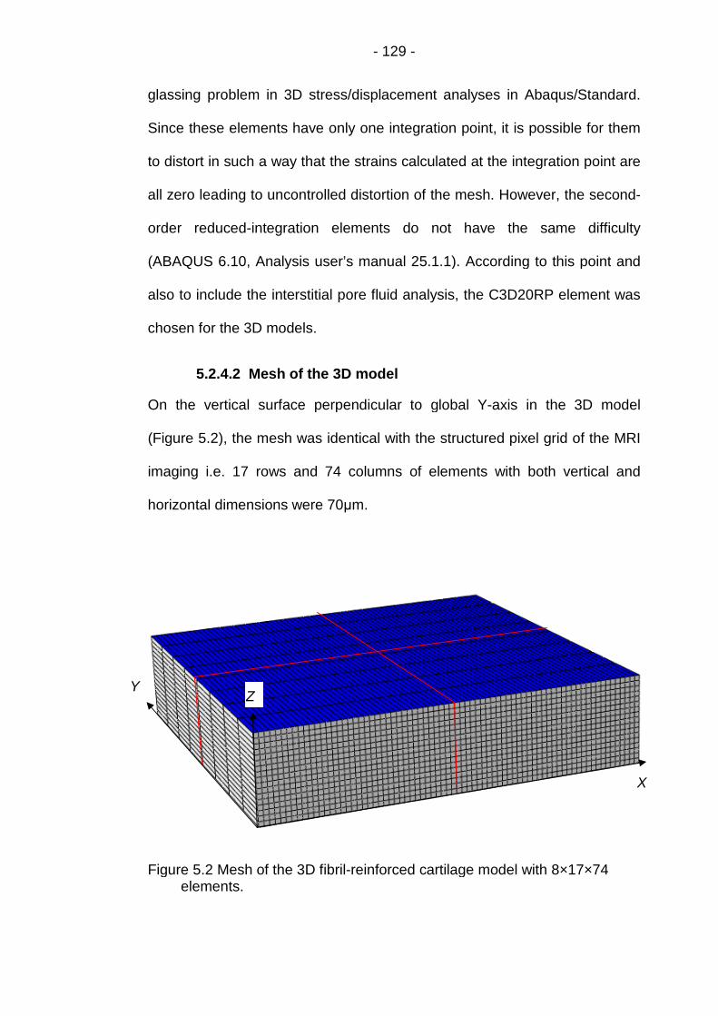
- 129 -
glassing problem in 3D stress/displacement analyses in Abaqus/Standard.
Since these elements have only one integration point, it is possible for them
to distort in such a way that the strains calculated at the integration point are
all zero leading to uncontrolled distortion of the mesh. However, the second-
order reduced-integration elements do not have the same difficulty
(ABAQUS 6.10, Analysis user’s manual 25.1.1). According to this point and
also to include the interstitial pore fluid analysis, the C3D20RP element was
chosen for the 3D models.
5.2.4.2 Mesh of the 3D model
On the vertical surface perpendicular to global Y-axis in the 3D model
(Figure 5.2), the mesh was identical with the structured pixel grid of the MRI
imaging i.e. 17 rows and 74 columns of elements with both vertical and
horizontal dimensions were 70μm.
Figure 5.2 Mesh of the 3D fibril-reinforced cartilage model with 8×17×74elements.
X
ZY

- 130 -
For the convenience to define the centre and midlines on the top surface of
cartilage, the element number along the cartilage edge parallel to the Y-axis
was designed to be even. In order to determine this specific number, mesh
sensitivity analysis was carried out.
5.2.5 Mesh sensitivity analysis of the 3D isotropic model
In order to analyze the mesh sensitivity on the peak value of fluid load
support, poroelastic material in Table 4.1 was employed in the 3D
axisymmetric isotropic FE model: Young’s modulus E = 0.69 MPa (Mononen
et al., 2010), the Poisson’s ratio ν = 0.36, the permeability k = 0.003 mm4/N∙s
and the initial void ratio e0 = 4.0 (Li et al., 2009). The model was
homogenous i.e. all material parameters were constant through the tissue
depth.
As the element numbers along the edge parallel to the X and Z-axis were
coincide to the MRI pixel grid (17 rows and 74 columns; Figure 5.1), the
mesh sensitivity analysis was performed by doubling the even number of
elements along the cartilage edge parallel to the Y-axis. In order to save the
computation time, ‘8’ was selected to be the initial number.
The 3D isotropic models with the mesh densities of 32×17×74 and
64×17×74 elements were too computationally intensive to be practical. So
only the results of two models with 8×17×74 (Figure 5.2) and 16×17×74
elements were compared:

- 131 -
(a)
(b)
(c)
Figure 5.3 Comparison of contact pressure (a), pore pressure (b) and fluidload support (c) at the centre of cartilage surface in isotropic modelswith different number of elements during the simulation (t=3600s).
The axial displacement of cartilage surface during the simulation is also
compared in Figure 5.4:
0
10
20
30
40
50
60
70
0 1000 2000 3000 4000C
on
tact
Pre
ssu
re(k
Pa)
Loading Time (s)
8x74 C3D20
16x74 C3D20
0
10
20
30
40
50
60
70
0 1000 2000 3000 4000
Po
reP
ress
ure
(kP
a)
Loading Time (s)
8x74 C3D20
16x74 C3D20
0
20
40
60
80
100
0 1000 2000 3000 4000
Flu
idLo
adSu
pp
ort
(%)
Loading Time (s)
8x74 C3D20
16x74 C3D20
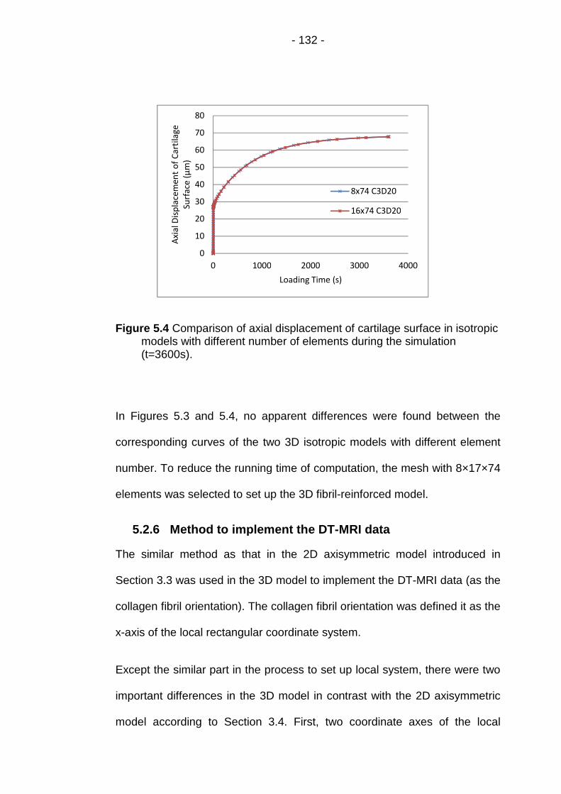
- 132 -
Figure 5.4 Comparison of axial displacement of cartilage surface in isotropicmodels with different number of elements during the simulation(t=3600s).
In Figures 5.3 and 5.4, no apparent differences were found between the
corresponding curves of the two 3D isotropic models with different element
number. To reduce the running time of computation, the mesh with 8×17×74
elements was selected to set up the 3D fibril-reinforced model.
5.2.6 Method to implement the DT-MRI data
The similar method as that in the 2D axisymmetric model introduced in
Section 3.3 was used in the 3D model to implement the DT-MRI data (as the
collagen fibril orientation). The collagen fibril orientation was defined it as the
x-axis of the local rectangular coordinate system.
Except the similar part in the process to set up local system, there were two
important differences in the 3D model in contrast with the 2D axisymmetric
model according to Section 3.4. First, two coordinate axes of the local
0
10
20
30
40
50
60
70
80
0 1000 2000 3000 4000
Axi
alD
isp
lace
men
to
fC
arti
lage
Surf
ace
(μm
)
Loading Time (s)
8x74 C3D20
16x74 C3D20
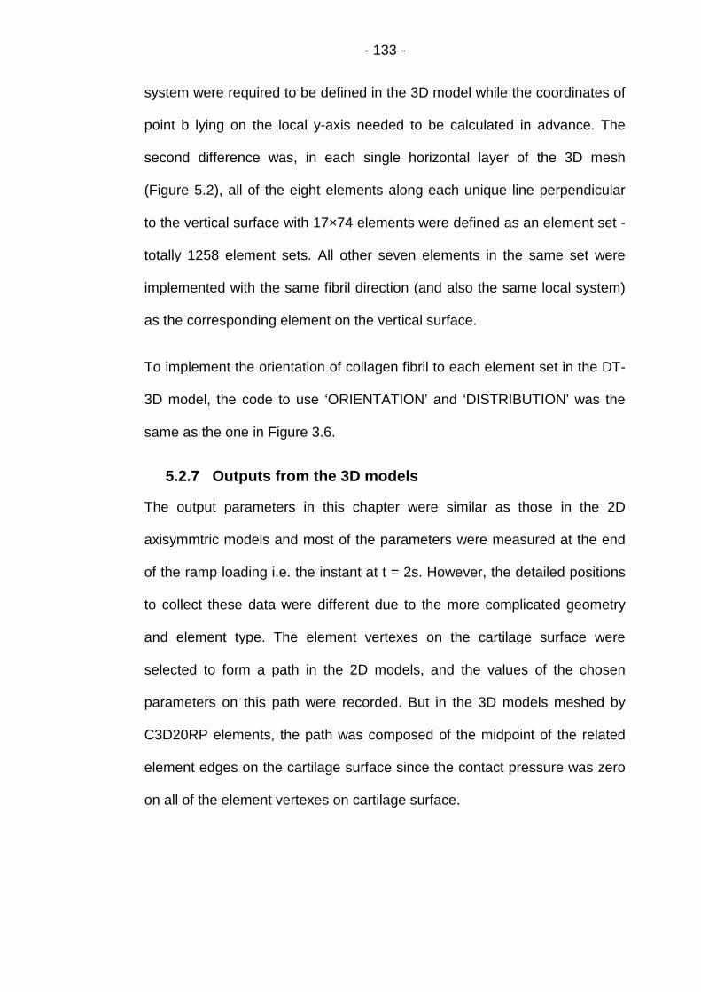
- 133 -
system were required to be defined in the 3D model while the coordinates of
point b lying on the local y-axis needed to be calculated in advance. The
second difference was, in each single horizontal layer of the 3D mesh
(Figure 5.2), all of the eight elements along each unique line perpendicular
to the vertical surface with 17×74 elements were defined as an element set -
totally 1258 element sets. All other seven elements in the same set were
implemented with the same fibril direction (and also the same local system)
as the corresponding element on the vertical surface.
To implement the orientation of collagen fibril to each element set in the DT-
3D model, the code to use ‘ORIENTATION’ and ‘DISTRIBUTION’ was the
same as the one in Figure 3.6.
5.2.7 Outputs from the 3D models
The output parameters in this chapter were similar as those in the 2D
axisymmtric models and most of the parameters were measured at the end
of the ramp loading i.e. the instant at t = 2s. However, the detailed positions
to collect these data were different due to the more complicated geometry
and element type. The element vertexes on the cartilage surface were
selected to form a path in the 2D models, and the values of the chosen
parameters on this path were recorded. But in the 3D models meshed by
C3D20RP elements, the path was composed of the midpoint of the related
element edges on the cartilage surface since the contact pressure was zero
on all of the element vertexes on cartilage surface.
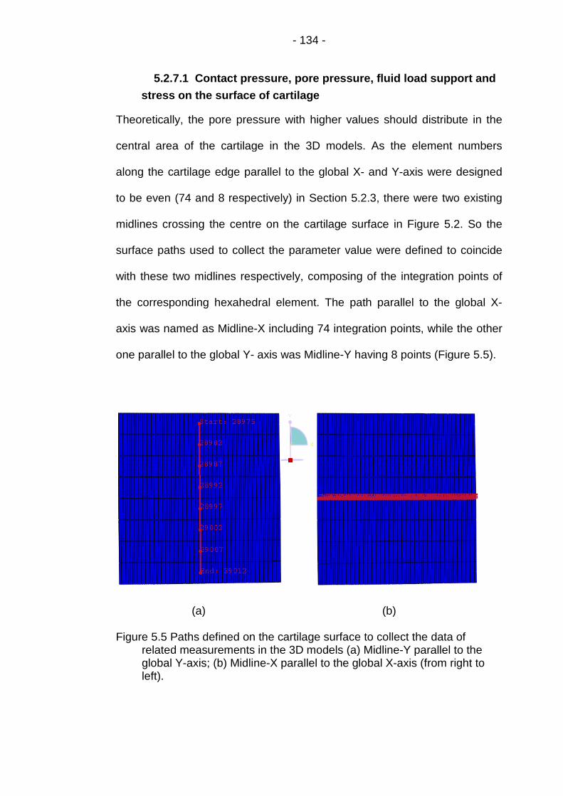
- 134 -
5.2.7.1 Contact pressure, pore pressure, fluid load support and
stress on the surface of cartilage
Theoretically, the pore pressure with higher values should distribute in the
central area of the cartilage in the 3D models. As the element numbers
along the cartilage edge parallel to the global X- and Y-axis were designed
to be even (74 and 8 respectively) in Section 5.2.3, there were two existing
midlines crossing the centre on the cartilage surface in Figure 5.2. So the
surface paths used to collect the parameter value were defined to coincide
with these two midlines respectively, composing of the integration points of
the corresponding hexahedral element. The path parallel to the global X-
axis was named as Midline-X including 74 integration points, while the other
one parallel to the global Y- axis was Midline-Y having 8 points (Figure 5.5).
(a) (b)
Figure 5.5 Paths defined on the cartilage surface to collect the data ofrelated measurements in the 3D models (a) Midline-Y parallel to theglobal Y-axis; (b) Midline-X parallel to the global X-axis (from right toleft).

- 135 -
5.2.7.2 The fluid velocity and contour of pore pressure
The fluid velocity (FLVEL) within the cartilage represents the direction and
magnitude of the interstitial fluid flow. The contour of pore pressure
illustrates the pressure distribution at various parts of the cartilage. In the 2D
axisymmetric models in Chapter 4, the distributions of these two parameters
could only be displayed in a two dimensional map representing the
distributions at any other parts of the realistic three dimensional cartilage.
This may be feasible in the homogeneous models such as isotropic (or
transversely isotropic) model. But for the non-homogeneous models,
particularly the fibril reinforced model implementing realistic fibril orientation,
it is unreasonable due to the anisotropic material properties of the tissue.
For the 3D models in this chapter, the distributions at any part inside
cartilage could be investigated directly by view-cutting (ABAQUS manual -
Getting Started) the 3D geometry of the tissue. The most frequently used
patterns to cut the cartilage are the two cross-sections along the two
midlines (red lines in Figure 5.6) and perpendicular to the global X- and Y-
axis respectively in the meantime.

- 136 -
(a)
(b)
Figure 5.6 Themeasuremperpendicto the glo
5.2.7.3
The vertic
Similar as in
deformation of
3D models in
the vertical de
crucial for the
not be same.
the difference
element. Inform
Mid
two cross-sections to investigate the distributions of relatedents inside cartilage in the 3D models: (a) the cross-section
ular to the global X-axis; (b) the cross-section perpendicularbal Y-axis.
Deformation of the cartilage
al deformation
the 2D axisymmetric models of Chapter 4, the vertical
the whole cartilage was set up to be the same in the different
order to make it reasonable to compare the results. However,
formation of the top layer elements of the cartilage, which was
investigation of fluid load support on the cartilage surface, may
The vertical deformation of a specific element was defined as
of the axial displacement of the top and bottom vertex of this
ation from the elements along the two midlines in Figure 5.5
Midline-Y
line-X

- 137 -
and the four edges of the cartilage surface were recorded and calculated to
represent the vertical deformation of the top layer of cartilage.
The radial deformation
In order to compare the radial deformation of cartilage in different 3D
models, another two midlines perpendicular to the horizontal surface on the
corresponding vertical surface were defined respectively in Figure 5.2 -
Midline-X-Z in the global X-Z plane perpendicular to Midline-X and Midline-
Y-Z perpendicular to Midline-Y in the global Y-Z plane.
5.3 Modelling Cases
Three dimensional models were set up with different material settings: the
realistic fibril orientation model with strain dependent fibrillar Young’s
modulus (named DT-MRI-3D); the Uniform reinforced model with constant
dependent fibrillar Young’s modulus (Uniform-3D model); and the basic
model with isotropic poroelastic material (Isotropic-3D) - totally three
modeling cases. The same geometry, mesh, boundary conditions and
loading were used in all of the three models. The material properties
employed in these models, including the collagen fibril orientation (except in
the Isotropic-3D model), are described in Table 5.1.
The value of the fibril Young’s modulus on the local x-axis, Efx, in the
Uniform-3D model had been adjusted to 4.0 MPa and Efy = Efz = 1.33 MPa
to match the vertical displacement of the cartilage surface centre in the DT-
MRI -3D model at the end of the ramp loading stage, in order to make the
comparison reasonable. The Young’s modulus Em was also adjusted in the

- 138 -
Isotropic model. To provide the information of the cartilage deformation to
carry out this adjustment, the DT-3D model was set up first.
Table 5.1 Material properties of different models (ε is the fibrillar strain ineach iteration and 4.0 represented 80% interstitial fluid).
Modelling case
Material parameter
DT-MRI -
3D
Uniform-
3D
Isotropic-
3D
Young’s modulus of nonfibrillar
matrix, Em (MPa)0.52 0.52 1.13
Poisson’s ratio of nonfibrillar
matrix, vm
0.36 0.36 0.36
Young’s modulus of fibril on
local x-axis, Efx (MPa)3+1600εx 4.0 n/a
Young’s modulus of fibril on
local y-axis, Efy (MPa)0.9+480εy 1.33 n/a
Young’s modulus of fibril on
local z-axis, Efz (MPa)0.9+480εz 1.33 n/a
Permeability, k (m4/N∙s) 3.0×10⁻¹⁵ 3.0×10⁻¹⁵ 3.0×10⁻¹⁵
Initial void ratio, e0 4.0 4.0 4.0
Source of fibril orientation DT-MRIManual
uniformn/a
5.3.1 The 3D fibril reinforced model
5.3.1.1 Mechanical property of material
In the DT-3D model, the Young’s modulus of the fibrillar network was
direction dependent and varied linearly with tensile strain but to be zero for
compression: Efx = 3 + 1600εx MPa; Efy = 0.9 + 480εy MPa; Efz = 0.9 + 480εz
MPa (Efx, Efy and Efz represent modulus in local x, y and z direction

- 139 -
respectively), εx, εy and εz is the fibrillar strain in local x, y and z direction as
described in Chapter 3. Efy and Efz were defined to simulate the tensile
stiffness of the collagen network produced by the cross-links (Kazemi et al.,
2011).
The material property of the nonfibrillar poroelastic matrix was same as the
2D fibril reinforced model except the Young’s modulus Em: isotropic with
Poisson’s ratio mߥ = 0.36, permeability k = 0.003 mm4/Ns and the initial void
ratio e0 = 4.0 (Li et al., 1999 and 2009). If 0.26 MPa was still used as the
value of Em, the fluid load support was higher than 100% at the end of ramp
loading (Figure 5.7) which was unreasonable at several integration points on
the Midline-X parallel to the global X-axis. When Em was increased to 0.52
MPa, all of the values of fluid load support were less than 100% (Figure 5.7).
Figure 5.7 Fluid load support along the Midline-X on cartilage surfaceparallel to the global X-axis in the DT-MRI-3D models with differentvalues of Young’s modulus Em of the nonfibrillar at the end of ramploading (t = 2s).
0
20
40
60
80
100
120
140
0 1.1 2.2 3.3 4.4 5.5
Flu
idLo
adSu
pp
ort
alo
ng
Mid
line-
X(%
)
Distance from the Start Point of Midline-X (mm)
DT-3D-0.26MPa
DT-3D-0.36MPa
DT-3D-0.52MPa

- 140 -
5.3.1.2 Implementation of fibril orientation
The user-defined “ORIENTATION” including “Distribution” introduced in
Section 3.4 was used to incorporate the fibril orientation in the DT-3D model.
Part of the detailed input file is displayed below:
*DISTRIBUTION TABLE, NAME=tab2COORD3D, COORD3D
*DISTRIBUTION, NAME=dist2, LOCATION=element, TABLE=tab2, aX0,aY0,aZ0,bX0,bY0,bZ0
element set name, X17,1, Y17,1, Z17,1,bX17,1,bY17,1,bZ17,1element set name, X17,2, Y17,2, Z17,2,bX17,2,bY17,2,bZ17,2
…
element set name, X17,74, Y17,74, Z17,74,bX17,74,bY17,74,bZ17,74element set name, X16,1, Y16,1, Z16,1,bX16,1,bY16,1,bZ16,1
…
element set name, X2,74, Y2,74, Z2,74,bX1,74,bY1,74,bZ1,74element set name, X1,1, Y1,1, Z1,1,bX2,1,bY2,1,bZ2,1
…
element set name, X1,74, Y1,74, Z1,74,bX1,74,bY1,74,bZ1,74*ORIENTATION, NAME=ORI, DEFINITION=COORDINATES
dist2
“Distribution” in the DT-3D model
As introduced in Section 5.2.4, the principal eigenvector of a specific
diffusion tensor was defined as the x-axis of the local Cartesian coordinates
of the corresponding element set: the three components (Xij, Yij and Zij; i = 1
∙∙∙ 17, j = 1 ∙∙∙ 74) of every single principal eigenvector were implemented to
the corresponding element set in Figure 5.2 to represent the fibril orientation
in all elements of this set.

- 141 -
Calculation of the coordinates of point b lying on the local y-axis
There were two steps to define the coordinates of the second local point b
for each element set in the “Distribution”. Firstly, the three coordinate
components of the point (bXij, bYij, bZij; i = 1 ∙∙∙ 17, j = 1 ∙∙∙ 74) should be
calculated in advance using Formula 3.9. Then, the components were input
to the corresponding element set.
5.3.2 The 3D uniformly reinforced model
5.3.2.1 Mechanical property of material
In order to make the vertical displacement at the cartilage surface centre of
the 3D uniformly reinforced models match the DT-MRI-3D model at the end
of the ramp loading stage, the values of the fibril Young’s modulus on the
local axes in this model had been adjusted (Figure 5.8) while the other
material parameters in Table 5.1 remained unchanged.
In Figure 5.8, only the curve of the Uniform-3D model with 4.0 MPa fibril
Young’s modulus Efx (and 1.33 MPa for Efy and Efz) could match the vertical
displacement of the cartilage surface of the DT-MRI-3D model at t = 2s. The
other material parameters in this model (Table 5.1) were same as the DT-
MRI-3D model. The user-defined subroutine “UMAT” was still used in this
model, although the Young’s modulus was constant.

- 142 -
Figure 5.8 Adjustments of Young’s modulus in the Uniform-3D model toachieve the same axial displacement of cartilage surface centre as DT-MRI-3D model at the end of ramp loading (t = 2s).
5.3.2.2 Definition of the local coordinate system
Similar as the 2D uniformly reinforced models in Section 4.3, no specific
orientation of collagen fibrils were implemented this 3D uniformly reinforced
model. The local Cartesian coordinate in each element was defined to be the
same as the global system. This effectively aligned the fibril orientation with
the global X-axis. Each element was given an equal, maximum
reinforcement in the local x-direction when the material model was modified
based on this orientation.
Instead of the user-defined “ORIENTATION” including “Distribution” in
Section 3.3, the ‘Keyword’ method was used to define the local system by
specifying the locations of points a and b directly (Abaqus Analysis User's
Manual 2.2.5). The detailed input file in this model to define the local
0
0.4
0.8
1.2
1.6
2
2.4
0 0.5 1 1.5 2
Car
tila
geD
efo
rmat
ion
alo
ng
Z-ax
is(%
)
Time of Ramp Loading (s)
DT-3D-0.52Mpa
Uni-3D-Ef3
Uni-3D-Ef4.2
Uni-3D-Ef4.0

- 143 -
Cartesian coordinate was the same as the one used in the 2D uniformly
reinforced models in Section 4.3:
*Orientation, name=Ori-1, DEFINITION=COORDINATES, SYSTEM=RECTANGULAR
1.0, 0.0, 0.0, 0.0, 1.0, 0.0
5.3.3 The isotropic poroelastic model
In order to produce the comparable results, the value of Young’s modulus E
in Table 5.1was increased to 1.13MPa from 0.69MPa in Section 5.2
(Mononen et al., 2010) while the other material parameters remained. This
adjustment made the vertical deformation of the cartilage surface centre in
the Isotropic-3D model match the DT-MRI-3D model at the end of the ramp
loading stage (Figure 5.9).
Figure 5.9 Adjustments of Young’s modulus in the Isotropic-3D model toachieve the same axial displacement of cartilage surface centre as theDT-MRI-3D model at the end of ramp loading (t = 2s).
0
0.4
0.8
1.2
1.6
2
2.4
0 0.5 1 1.5 2
Car
tila
geD
efo
rmat
ion
alo
ng
Z-ax
is(%
)
Time of Ramp Loading (s)
DT-3D-0.52Mpa
Iso-3D-0.9MPa
Iso-3D-1.1MPa
Iso-3D-1.2MPa
Iso-3D-1.13MPa

- 144 -
5.4 Validation of the 3D DT-MRI based model
The MRI experimental data used in this project was generated from tests
performed by Robin Damon (School of Physics, University of Leeds), a
creep test (unconfined compression) were carried out on the cartilage
sample for 37.5 minutes under 0.2 MPa pressure after the acquirement of
the diffusion tensor, using a 9.5T MRI machine in the School of Physics and
Astronomy. Cartilage thickness was recorded during the loading period. The
measurement was performed using the AnalyzeTM image analysis software.
According to the experimental record, the initial cartilage thickness was
1355μm (slightly thinner that the result of 1.36 mm in Fermor et al., 2013).
This is not consistent with the corresponding data in the 3D DT-MRI model
which was 1190μm. In order to validate the 3D DT-MRI model, the data of
cartilage thickness was transformed to the information of the vertical
displacement of cartilage surface i.e. the vertical cartilage deformation and
normalized. The original deformation value at a specific time of the cartilage
sample was defined as the difference between the initial value and the value
corresponding to this time in the thickness record. Then the deformation
values were normalized as a percentage i.e. divided by the initial thickness
of cartilage (1355μm). Finally, the curve of the normalized vertical
displacement of cartilage surface during the creep test was produced (Figure
5.10).
In Figure 5.10, the vertical deformation of the cartilage sample did approach
the equilibrium which was slightly higher than 18% at the last stage of the
creep test. The validation of the DT-MRI-3D model was carried out by curve-
fitting this experimental result.

- 145 -
Figure 5.10 Normalized vertical displacements (%) of cartilage surface in thecreep test.
In order to perform the validation, the value of the Young’s modulus of the
nonfibrillar matrix Em in the DT-MRI-3D model (Table 5.1) was increased to
enable the cartilage to support the higher applied load equivalent to the
applied pressure (0.2 MPa) in the experiment.
As the permeability k used in the previous models in this thesis was
3.0×10⁻¹⁵ m4/(N∙s) which was cited from Li et al. (2009). This value was in
the typical range of ~ 0.1-10×10−15 m4/(Ns) for permeability of articular
cartilage (Chen et al., 2001; Frank et al., 1987; Jurvelin et al., 2003; Mow et
al., 1984). However, the permeability of cartilage from bovine groove was
determined as 0.663×10⁻¹⁵ m4/(Ns) according to the latest measurement of
Fermor et al. (2013). So the value of permeability was also adjusted to
0
2
4
6
8
10
12
14
16
18
20
0 250 500 750 1000 1250 1500 1750 2000 2250
Axi
alD
efo
rmat
ion
of
Car
tila
ge(%
)
Loading Time (s)

- 146 -
investigate its effects on the modelling results of cartilage deformation and
the curve-fitting of the experimental data.
5.5 Results
The results from different modelling cases described in Section 5.3 are
collected and compared to each other in the first subsection. The validation
results are displayed separately in the second subsection.
5.5.1 Comparison of results from different 3D models
5.5.1.1 Contact pressure, pore pressure and fluid load support
on the cartilage surface
Comparison of contact pressure along midlines of the cartilage surface
The value of contact pressure was highest in the central parts of the midlines
and decreased to the parts near the edges in all of the three models (Figure
5.11), while the curve along Midline-X of the DT-MRI-3D model fluctuated
frequently (Figure 5.11(a)). The Isotropic model had the highest values along
Midline-Y (Figure 5.11 (b)).

- 147 -
(a)
(b)
Figure 5.11 Comparison of contact pressure on the cartilage surface along(a) Midline-X and (b) Midline-Y at the end of ramp loading (t = 2s).
Comparison of pore pressure along midlines of the cartilage surface
Similar as the distribution of contact pressure, the value of pore pressure
was also higher in the central parts of the midlines than in the parts aside
while the curves of the Isotropic-3D model were lowest along both midlines
(Figure 5.12). The curves of the DT-MRI-3D model had the highest values
although fluctuated along Midline-X (Figure 5.12 (a)).
0
10
20
30
40
50
60
70
0 1.3 2.6 3.9 5.2
Co
nta
ctP
ress
ure
alo
ng
MId
line-
X(k
Pa)
Distance from Start Point of Midline-X (mm)
DTMRI-3D
Uniform-3D
Isotropic-3D
0
10
20
30
40
50
60
70
0 1 2 3 4 5
Co
nta
ctP
ress
ure
alo
ng
Mid
line-
Y(k
Pa)
Distance from Start Point of Midline-Y (mm)
DT-MRI-3D
Uniform-3D
Isotropic-3D

- 148 -
(a)
(b)
Figure 5.12 Comparison of pore pressure on the cartilage surface along (a)Midline-X and (b) Midline-Y at the end of ramp loading (t = 2s).
Comparison of fluid load support along midlines of the cartilage
surface
Except on the limited number of points along Midline-X, the values of fluid
load support of the DT-MRI-3D model were higher than the corresponding
value of the other two models as expected (Figure 5.13 (a)). The curves of
the Isotropic-3D were the lowest with values less than 65% (Figure 5.13).
0
10
20
30
40
50
60
0 1.3 2.6 3.9 5.2Po
reP
ress
ue
alo
ng
Mid
line-
X(k
Pa)
Distance from Start Point of Midline-X (mm)
DT-MRI-3D
Uniform-3D
Isotropic-3D
0
10
20
30
40
50
60
0 1 2 3 4 5
Po
reP
ress
ure
alo
ng
Mid
line-
Y(k
Pa)
Distance fron Start Point of Midlind-Y (mm)
DT-MRI-3D
Uniform-3D
Isotropic-3D

- 149 -
(a)
(b)
Figure 5.13 Comparison of fluid load support on the cartilage surface along(a) Midline-X and (b) Midline-Y at the end of ramp loading (t = 2s).
Distribution of contact pressure on the cartilage surface
Calculated only on the integration points of the reduced hexahedral element,
contact pressure distributed discontinuously with the higher values at the
central area of the cartilage surface and decreased to the region near the
edges in all of the three models (Figure 5.14).
0
10
20
30
40
50
60
70
80
90
100
0 1.3 2.6 3.9 5.2Flu
idLo
adSu
pp
ort
alo
ng
Mid
line-
X(%
)
Distance from the Start Point of Midline-X (mm)
DT-MRI-3D
Uniform-3D
Isotropic-3D
0
10
20
30
40
50
60
70
80
90
100
0 1 2 3 4 5
Flu
idLo
adSu
pp
ort
alo
ng
Mid
line-
Y(%
)
Distance from the Start Point of Midline-Y (mm)
DT-MRI-3D
Uniform-3D
Isotropic-3D
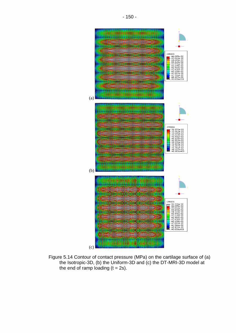
- 150 -
(a)
(b)
(c)
Figure 5.14 Contour of contact pressure (MPa) on the cartilage surface of (a)the Isotropic-3D, (b) the Uniform-3D and (c) the DT-MRI-3D model atthe end of ramp loading (t = 2s).

- 151 -
Distribution of pore pressure on the cartilage surface (Figure 5.15)
(a)
(b)
(c)
Figure 5.15 Contour of pore pressure (MPa) on the cartilage surface of (a)the Isotropic-3D, (b) the Uniform-3D and (c) the DT-MRI-3D at the endof ramp loading (t = 2s).

- 152 -
The region with higher pore pressure around the cartilage surface centre
was much smaller in the Isotropic-3D model than in the Uniform-3D model
(brown area in Figure 5.15 (a) and (b)). Only in the DT-MRI-3D model, the
highest values of pore pressure emerged on the cartilage surface (central
region with grey and red colour in Figure 5.15 (c)).
Inside distribution of pore pressure on the cross-section of cartilage
perpendicular to the global X-axis
The highest value of pore pressure arose at different position of the cartilage
bottom in the three models (Figure 5.16). Different from the two simpler
models, the pore pressure with the second highest value also emerged from
the middle zone to the surface of cartilage (the upper red area in Figure 5.16
(c)) in the DT-MRI-3D model.
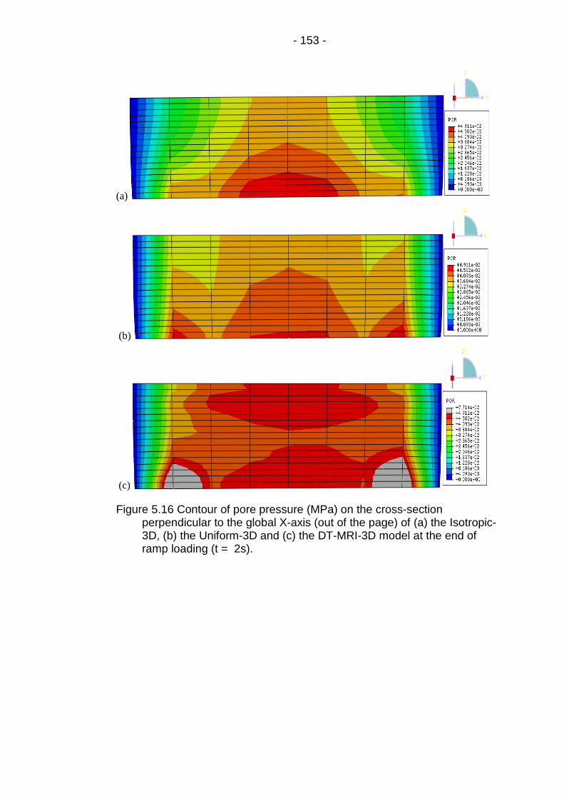
- 153 -
(a)
(b)
(c)
Figure 5.16 Contour of pore pressure (MPa) on the cross-sectionperpendicular to the global X-axis (out of the page) of (a) the Isotropic-3D, (b) the Uniform-3D and (c) the DT-MRI-3D model at the end oframp loading (t = 2s).

- 154 -
Inside distribution of pore pressure on cross section of cartilage
perpendicular to the global Y-axis (Figure 5.17)
(a)
(b)
(c)
Figure 5.17 Contour of pore pressure (MPa) on the cross-sectionperpendicular to the global Y-axis (out of the page) of (a) the Isotropic-3D, (b) the Uniform-3D and (c) the DT-MRI-3D model at the end oframp loading (t = 2s).

- 155 -
In the Isotropic-3D and Uniform-3D model, the highest value of pore
pressure only arose around the centre of cartilage bottom (red region in
Figure 5.17 (a) and (b)). But in the DT-MRI-3D model, the highest pore
pressure also distributed in the whole central area of the tissue from the
surface to the bottom (grey and red region in Figure 5.17 (c)).
Contact pressure, pore pressure and fluid load support at cartilage
surface centre during the loading period
Although the peak values of contact pressure were similar in the three
models, the peak pore pressure was much higher in the DT-MRI-3D model
than in the other two models leading to the highest peak fluid load support
(Figure 5.18). The pore pressure and fluid load support decreased similarly
after ramp load and tended to zero while the load was maintained.

- 156 -
Figure 5.18 Comparison of fluid load support at cartilage surface centreduring the loading period (t = 3602s).
0
10
20
30
40
50
60
70
0 601 1202 1803 2404 3005 3606
Co
nta
ctP
ress
ure
on
Car
tila
geSu
rfac
eC
entr
e(K
Pa)
Loading Time (s)
DT-MRI-3D
Uniform-3D
0
10
20
30
40
50
60
0 601 1202 1803 2404 3005 3606Po
reP
ress
ure
on
Car
tila
geSu
rfac
eC
entr
e(K
Pa)
Loading Time (s)
DT-MRI-3D
Uniform-3D
0
10
20
30
40
50
60
70
80
90
100
0 601 1202 1803 2404 3005 3606
Flu
idLo
adSu
pp
ort
on
Car
tila
geSu
rfac
eC
entr
e(%
)
Loading Time (s)
DT-MRI-3D
Uniform-3D

- 157 -
5.5.1.2 Distribution of fluid velocity
Distribution of fluid velocity on the vertical outer sides surfaces of
cartilage (Figure 5.19)
(a)
(b)
(c)
Figure 5.19 Distribution of fluid velocity (mm/s) on the vertical outer sides ofcartilage in (a) the Isotropic-3D, (b) the Uniform-3D and (c) the DT-MRI-3D model at the end of ramp loading (t = 2s).
On the vertical sides perpendicular to the global X-axis, the Unifrom-3D
model had the largest fluid velocity (Figure 5.19 (b)); the Isotropic-3D model

- 158 -
had similar distribution near the cartilage bottom as the DT-MRI-3D model
but less magnitude from the middle area to the cartilage surface (Figure 5.19
(a) and (c)). On the two vertical sides perpendicular to the global Y-axis, fluid
flew out only near the bottom of the tissue while increasing with the
complexity of the material, although the magnitude was much lower than that
on the adjacent sides (Figure 5.19).
Inside distribution of fluid velocity on the cross section of cartilage
perpendicular to the global X-axis
In each individual model in Figure 5.20, the distribution of fluid velocity
decreased from the outer edges to the central part of the cross section of
cartilage perpendicular to the global X-axis. Compared to the other two
models, the Unifrom-3D model had the lowest inside fluid velocity on the
section (Figure 5.20).

- 159 -
(a)
(b)
(c)
Figure 5.20 Distribution of fluid velocity (mm/s) on the cross-sectionperpendicular to the global X-axis (out of the page) of (a) the Isotropic-3D, (b) the Uniform-3D and (c) the DT-MRI-3D model at the end oframp loading (t = 2s).

- 160 -
Inside distribution of fluid velocity on the cross section of cartilage
perpendicular to the global Y-axis (Figure 5.21 )
(a)
(b)
(c)
Figure 5.21 Distribution of fluid velocity (mm/s) on the cross-sectionperpendicular to the global Y-axis (out of the page) of (a) the Isotropic-3D, (b) the Uniform-3D and (c) the DT-MRI- 3D model at the end oframp loading (t = 2s).
The Unifrom-3D model also had the lowest inside fluid velocity on the cross
section of cartilage perpendicular to the global Y-axis (Figure 5.21 (b)). Fluid

- 161 -
velocity inside the Isotropic model distributed much more regularly in
contrast to the disorder distribution in the DT-MRI-3D model (Figure 5.21 (a)
and (c)).
5.5.1.3 Deformation of the cartilage
Radial deformation of cartilage along Midline-X-Z and Midline-Y-Z
(Figure 5.22)
(a)
(b)
Figure 5.22 Comparison of radial deformation of cartilage on the direction of(a) global X-axis and (b) global Y-axis at the end of ramp loading (t =2s).
0
2
4
6
8
10
12
14
16
18
0 0.2 0.4 0.6 0.8 1
Nu
mb
ero
fN
od
eso
nM
idlin
e-Y-
Z(f
rom
Car
tila
geSu
rfac
eto
Bo
tto
m)
Radial Displacement on the Direction of Global X-axis (%)
DT-MRI-3D
Uniform-3D
Isotropic-3D
1
3
5
7
9
11
13
15
17
0 0.2 0.4 0.6 0.8 1
Nu
mb
ero
fN
od
eso
nM
idlin
e-X
-Z(f
rom
Surf
ace
toB
ott
om
)
Radial Displacement on the Direction of Global Y-axis (%)
DT-MRI-3D
Uniform-3D
Isotropic-3D

- 162 -
For the DT-MRI-3D model, radial displacement along the global X-axis of
points on Midline-Y-Z was higher than the value of the corresponding points
in the Uniform-3D model (Figure 5.22 (a)); but the values along the global Y-
axis on Midline-X-Z were lower than the Uniform-3D model (Figure 5.22 (b)).
Vertical deformation of cartilage layers along Midline-X-Z and Midline-
Y-Z (Figure 5.23)
Along both Midline-X-Z and Midline-Y-Z, the vertical deformation of the first
cartilage layer in the DT-MRI-3D model was larger than in the other two
models (Figure 5.23). The curves in this figure only represented the
information of the central region of cartilage and were not enough to
investigate the effect on the interstitial fluid pressurization in the whole first
layer of cartilage. More data on the vertical deformation of the first cartilage
layer were collected below, along the two midlines and edges of the cartilage
surface.

- 163 -
(a)
(b)
Figure 5.23 Comparison of vertical deformation of cartilage layers along (a)Midline-Y-Z and (b) Midline-X-Z at the end of ramp loading (t = 2s).
1
3
5
7
9
11
13
15
17
0 0.1 0.2 0.3 0.4 0.5 0.6
Nu
mb
ero
fC
arti
lage
Laye
r(f
rom
Surf
ace
toB
ott
om
)
Vertical Deformation along Midline Y-Z (%)
DT-MRI-3D
Uniform-3D
Isotropic-3D
1
3
5
7
9
11
13
15
17
0 0.2 0.4 0.6 0.8
Nu
mb
ero
fN
od
eso
nM
idlin
e-X
-Z(f
rom
Surf
ace
toB
ott
om
)
Vertical Deformationt (%)
DT-MRI-3D
Uniform-3D
Isotropic-3D

- 164 -
The vertical deformation of elements along Midline-X and the two
cartilage surface edge in global X-Z plane (Figure 5.24; next page).
(a)
(b)
(c)
Figure 5.24 Comparison of vertical deformation of elements along Midline-Xand the two cartilage surface edge in global X-Z plane at the end oframp loading (t = 2s).
0
0.03
0.06
0.09
0.12
0.15
0.18
0 15 30 45 60 75
Def
orm
atio
no
fV
erti
calE
lem
ent
Edge
ss(%
)
Number of Vertical Edge of Outter Surface Elements inthe Top Cartilage Layer in X-Z Plane
DT-MRI-3DUniform-3DIsotropic-3D
0
0.03
0.06
0.09
0.12
0.15
0.18
0.21
0.24
0 15 30 45 60 75Def
orm
atio
no
fV
erti
calE
lem
ent
Edge
s(%
)
Number of Vertical Element Edge along Midline-X
DT-MRI-3D
Uniform-3D
Isotropic-3D
-0.03
0
0.03
0.06
0.09
0.12
0.15
0 15 30 45 60 75
Def
orm
atio
no
fV
erti
calE
lem
ent
Edge
s(%
)
Number of Vertical Edge of Outter Surface Elements inthe Top Cartilage Layer in X-Z Plane
DT-MRI-3DUniform-3DIsotropic-3D

- 165 -
For the DT-MRI-3D model, the deformation of the vertical edges of most
elements was apparently higher along both of the cartilage surface edges in
global X-Z plane (Figure 5.24 (a) and (c)) but lower than in the other two
models along Midline-X (Figure 5.24 (b)).
Vertical deformation of elements along Midline-Y and the two
cartilage surface edge in global Y-Z plane
The deformation of the vertical edges of elements along Midline-Y was
similar nearly coincide in the three models; and the differences between the
values in the DT-MRI-3D and Uniform-3D model were not so apparent small
(Figure 5.25) as those in Figure 5.24.

- 166 -
(a)
(b)
(c)
Figure 5.25 Comparison of vertical deformation of cartilage layers in globalY-Z plane at the end of ramp loading (t = 2s).
0
0.03
0.06
0.09
0.12
0.15
0 3 6 9Def
orm
atio
no
fV
erti
calE
lem
ent
Edge
s(%
)
Number of Vertical Edge of Outter Surface Elements in theTop Cartilage Layer in Y-Z Plane
DT-MRI-3D
Uniform-3D
Isotropic-3D
0
0.03
0.06
0.09
0.12
0.15
0.18
0 3 6 9
Def
orm
atio
no
fV
erti
calE
lem
ent
Edge
s(%
)
Number of Vertical Element Edge along Midline-Y
DT-MRI-3D
Uniform-3D
Isotropic-3D
-0.03
0
0.03
0.06
0.09
0.12
0.15
0 3 6 9Def
orm
atio
no
fV
erti
calE
lem
ent
Edge
s(%
)
Number of Vertical Edge of Outter Surface Elements in theTop Cartilage Layer in Y-Z Plane
DT-MRI-3D
Uniform-3D
Isotropic-3D

- 167 -
Vertical displacement of cartilage surface centre during loading period
The normalized vertical displacement of cartilage surface centre was
compared across three models during the full loading period (Figure 5.26).
After one hour’s creep all models had reached equilibrium.
Figure 5.26 Comparison of vertical displacement of cartilage surface centreduring loading period.
5.5.1.4 Stress on the cartilage surface
Stress along Midline-X (S11) and Midline-Y (S22)
The highest values of stress (S11) along Midline-X of cartilage surface
distributed in the central area and decreased to the parts near the edges in
all of the three models, although the curve in the DT-MRI-3D model
fluctuated severely (Figure 5.27(a)). The value of stress along Midline-Y
(S22) increased with the complexity of the material (Figure 5.27(b)).
0
1
2
3
4
5
6
0 601 1202 1803 2404 3005 3606
Ver
tica
lDis
pla
cem
ent
of
Car
tila
geSu
rfac
eC
entr
e(%
)
Loading Time (s)
DT-MRI-3D
Uniform-3D
Isotropic-3D
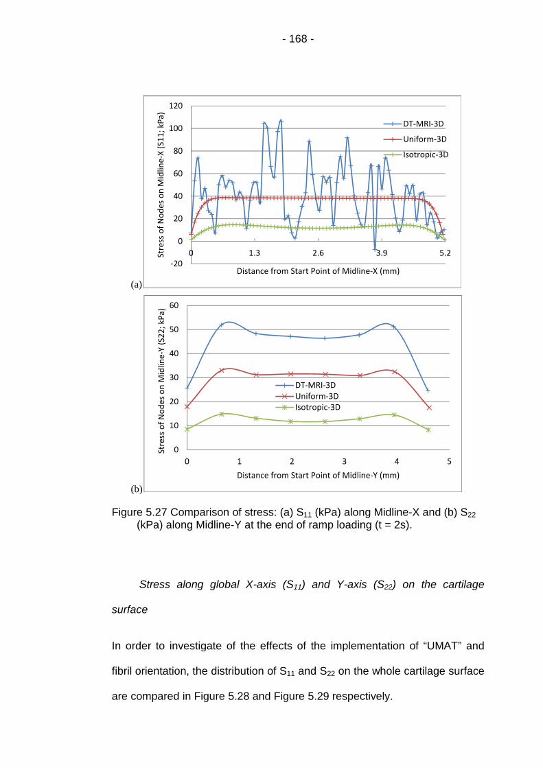
- 168 -
(a)
(b)
Figure 5.27 Comparison of stress: (a) S11 (kPa) along Midline-X and (b) S22
(kPa) along Midline-Y at the end of ramp loading (t = 2s).
Stress along global X-axis (S11) and Y-axis (S22) on the cartilage
surface
In order to investigate of the effects of the implementation of “UMAT” and
fibril orientation, the distribution of S11 and S22 on the whole cartilage surface
are compared in Figure 5.28 and Figure 5.29 respectively.
-20
0
20
40
60
80
100
120
0 1.3 2.6 3.9 5.2Stre
sso
fN
od
eso
nM
idlin
e-X
(S1
1;
kPa)
Distance from Start Point of Midline-X (mm)
DT-MRI-3D
Uniform-3D
Isotropic-3D
0
10
20
30
40
50
60
0 1 2 3 4 5
Stre
sso
fN
od
eso
nM
idlin
e-Y
(S2
2;
kPa)
Distance from Start Point of Midline-Y (mm)
DT-MRI-3DUniform-3DIsotropic-3D
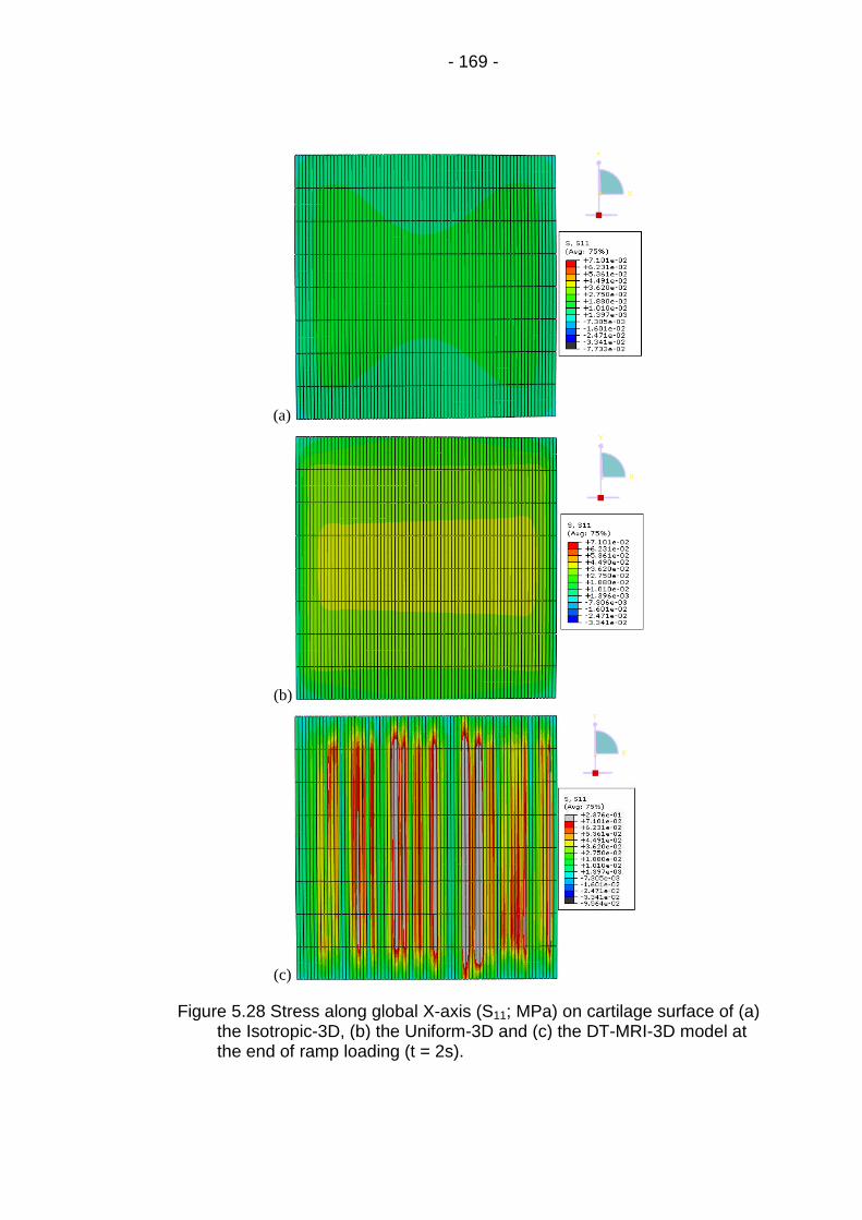
- 169 -
(a)
(b)
(c)
Figure 5.28 Stress along global X-axis (S11; MPa) on cartilage surface of (a)the Isotropic-3D, (b) the Uniform-3D and (c) the DT-MRI-3D model atthe end of ramp loading (t = 2s).

- 170 -
(a)
(b)
(c)
Figure 5.29 Stress along global Y-axis (S22; MPa) on cartilage surface of (a)the Isotropic-3D, (b) the Uniform-3D and (c) the DT-MRI-3D model atthe end of ramp loading (t = 2s).
In the DT-MRI-3D model, highest values of S11 and S22 distributed in narrow
stripes along global Y-axis (grey and red area in Figure 5.28 (c) and Figure
- 171 -
5.29 (c)) separated by the stripes with low values (green and blue area in
Figure 5.28 (c) and Figure 5.29 (c)). In contrast, S11 and S22 distributed
regularly in the Isotropic-3D and Uniform--3D model with higher values in the
central region ((a) and (b) in Figure 5.27 and Figure 5.29).
5.5.2 Validation results of the 3D DT-MRI based model
In order to enable the cartilage to support the higher load equivalent to the
applied pressure which was 0.2 MPa in the experiment, the Young’s
modulus of the nonfibrillar matrix Em in the DT-3D model were increased to
the range of 0.63 - 0.99 MPa from the value of 0.26 MPa in Table 5.1. The
axial displacements of the 3D-DT models with different Young’s modulus
were compared with the result of experiment (Figure 5.30).
In Figure 5.30, the curve of the DT-3D model with the Young’s modulus of
the nonfibrillar matrix Em = 0.66 MPa fitted the experimental data (blue
curve) better than the green curve with 0.63 MPa Young’s modulus at the
stage of equilibrium. The purple curve with 0.96 MPa Young’s modulus could
not follow the increase trend of the experimental data and achieved a much
lower equilibrium.
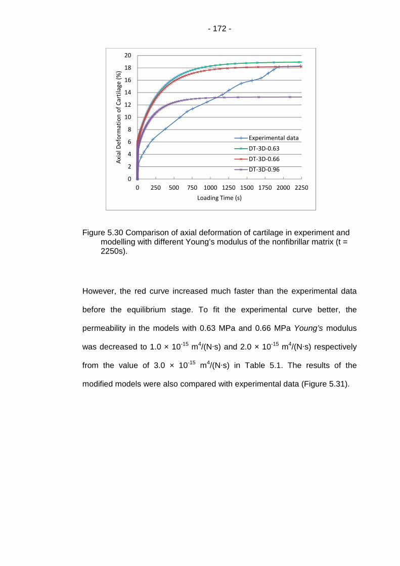
- 172 -
Figure 5.30 Comparison of axial deformation of cartilage in experiment andmodelling with different Young’s modulus of the nonfibrillar matrix (t =2250s).
However, the red curve increased much faster than the experimental data
before the equilibrium stage. To fit the experimental curve better, the
permeability in the models with 0.63 MPa and 0.66 MPa Young’s modulus
was decreased to 1.0 × 10⁻¹⁵ m4/(N∙s) and 2.0 × 10⁻¹⁵ m4/(N∙s) respectively
from the value of 3.0 × 10⁻¹⁵ m4/(N∙s) in Table 5.1. The results of the
modified models were also compared with experimental data (Figure 5.31).
0
2
4
6
8
10
12
14
16
18
20
0 250 500 750 1000 1250 1500 1750 2000 2250
Axi
alD
efo
rmat
ion
of
Car
tila
ge(%
)
Loading Time (s)
Experimental data
DT-3D-0.63
DT-3D-0.66
DT-3D-0.96

- 173 -
Figure 5.31 Comparison of axial deformation of cartilage in experiment andmodelling with different Young’s modulus and permeability of thenonfibrillar matrix (t = 2250s).
In contrast to the modelling results in Figure 5.30, the lower value of
permeability reduced the axial displacement of cartilage surface in the four
models in Figure 5.31 at the corresponding time. This made the two
modelling curves fit the experimental data better at the long period before
the equilibrium stage of creep test (Figure 5.31).
5.6 Discussion
The numerical results from the 3D fibril reinforced models in this chapter
(Section 5.5) modeled the functional role of collagen fibril in unconfined
compression of articular cartilage: the high tensile stiffness of collagen acts
in a similar way as the rigid side-wall of a confining chamber, resisting lateral
expansion of the tissue and pressurizing the interstitial fluid considerably to
0
2
4
6
8
10
12
14
16
18
20
0 250 500 750 1000 1250 1500 1750 2000 2250
Axi
alD
efo
rmat
ion
of
Car
tila
ge(%
)
Loading Time (s)
Experimental data
DT-3D-0.63-P1
DT-3D-0.66-P1
DT-3D-0.63-P2
DT-3D-0.66-P2

- 174 -
produce the pore pressure higher than that in the Isotropic model (Soltz and
Ateshian, 2000).
5.6.1 The effect of fibril reinforcement
5.6.1.1 The effect on pore pressure and fluid load support on
the cartilage surface
When the collagen fibrils were implemented by “UMAT”, the vertical Young’s
modulus in the DT-MRI-3D model was defined lower (0.52 MPa of non-
fibrillar Young’s modulus) than in the Isotropic-3D model (1.13 MPa). This
made the top layer of the tissue deform larger along the vertical direction in
the DT-MRI-3D model (Figures 5.23-5.25) and the interstitial fluid in the top
cartilage layer was pressurized more severely at the ramp loading stage,
compared to the Isotropic-3D model.
Meanwhile, the combined Young’s modulus in the radial direction (3 MPa of
fibrillar tensile modulus plus 0.52 MPa of non-fibrillar Young’s modulus)
which was much greater than that in the Isotropic-3D model (1.13 MPa) at
the beginning of simulation. As the fibrillar modulus was strain-dependent in
the DT-MRI-3D model, it increased as the cartilage was expanded while the
ramp load applied. The higher tensile modulus produced the higher values of
stress along the two midlines (S11 in Figure 5.27(a) except few lower points
and S22 in Figure 5.27(b)) and distributing on the whole cartilage surface
(Figure 5.28 and 5.29), leading to the lower deformation of the top cartilage
layer along the two radial direction of global X- and Y-axis in the DT-MRI-3D
model than in the Isotropic-3D model (Figure 5.22). The pressurization of the
interstitial fluid in the top cartilage layer was greatly enhanced by the lower
radial deformation. So the highest pore pressure (Figure 5.12 and 5.15) and

- 175 -
fluid load support (Figure 5.13) was produced in the DT-MRI-3D model in
contrast to the other two models.
As all of the collagen fibrils were aligned along the global X-axis and the
fibrillar Young’s modulus was constant but not strain-dependent as that in
the DT-MRI-3D model, the cartilage in the Uniform-3D model was not
reinforced to the similar extent as in the DT-MRI-3D model in the direction of
global Y-axis (Figure 5.29 (b) and (c)). This led to the greatly lower radial
deformation of the top cartilage layer in the direction of global X-axis (Figure
5.22(a)), and the slightly higher deformation along the global Y-axis (Figure
5.22(b)) compared to the Isotropic-3D model. But the vertical deformation of
the top cartilage layer was higher in the Uniform-3D model than in the
Isotropic-3D model particularly at regions near the surface edge (Figure
5.24-5.25) due to the lower vertical Young’s modulus compared to that in the
Isotropic-3D model. All these factors caused by fibril implementation
combined together, and produced the relatively higher pore pressure (Figure
5.12 and 5.15) and fluid load support (Figure 5.13) in the Uniform-3D model
than in the Isotropic-3D model.
5.6.1.2 The effect on pore pressure and fluid velocity inside the
whole cartilage
As the vertical deformation of the cartilage surface centre was set up to be
the same in all of the 3D models in Section 5.3, the radial deformation of the
whole cartilage became the main factor to affect the pressurization of the
interstitial fluid inside the tissue.
For the DT-MRI-3D model, the radial deformation was slightly higher in the
direction of global X-axis (Figure 5.22(a)) but apparently lower along the

- 176 -
global Y-axis (Figure 5.22(b)) than the Isotropic-3D model. This made the
pore pressure distribute completely different inside the whole cartilage in the
two models: the pore pressure with high values only arose around the centre
of cartilage bottom in the Isotropic-3D model ((a) in Figure 5.16 and 5.17);
but in the DT-MRI-3D model, it emerged from the middle zone to the surface
of cartilage ((c) in Figure 5.16 and 5.17) due to the reinforcement of the
collage fibril in the top two layers of cartilage.
The Uniform-3D model had the greatly lower radial deformation of the whole
cartilage in the direction of global X-axis although decreasing from top to
bottom (Figure 5.22(a)), compared to the Isotropic-3D model. This
reinforcement caused by the collagen fibril produced the second and third
highest pore pressure occupying the majority of the volume of cartilage in
the Uniform-3D model, particularly in the cross-section along the global Y-
axis ((b) in Figure 5.16 and 5.17).
Inside the cartilage, the differences of pore pressure at the various parts of
cartilage made the interstitial fluid flow from the parts with higher pore
pressure to the other parts where pore pressure was lower. So the different
distribution of pore pressure determined the magnitude and direction of the
fluid velocity in the three models. In the Isotropic-3D model, the regular
distribution of pore pressure with the high value in the central area of
cartilage ((a) in Figure 5.16 and 5.17) made the fluid flow outward while the
highest fluid velocity emerged along the bottom edge of cartilage parallel to
the global Y-axis ((a) in Figures 5.19 - 5.21). The widely distributing high
pore pressure in the Uniform-3D model ((b) in Figure 5.16 and 5.17)
produced the largest magnitude of fluid velocity on the vertical cartilage

- 177 -
surface in the global Y-Z plane ((b) in Figure 5.18 and 5.21), but it also
caused the lowest fluid velocity in the central volume of cartilage due to the
small differences of pore pressure in this region. As for the DT-MRI-3D
model, the irregular distribution of pore pressure ((c) in Figure 5.16 and 5.17)
led to the disordered fluid flow throughout the whole cartilage ((c) in Figure
5.19 - 5.21).
5.6.2 The influence of the realistic fibril orientation
Compared to the uniformly reinforced model, the implementation of the
realistic fibril orientation in the 3D fibril-reinforced model increased the value
of peak pore pressure by 15% while the peak contact pressure was 4.3%
lower, making the peak value of fluid load support increase from 80.4% to
96.7% (Figure 5.18). While the higher peak pore pressure decreased the
load supported by the solid phase of the cartilage, the lower value of peak
contact pressure would directly reduce the effective coefficient of friction and
protect the cartilage. These results were extremely different from those in
the 2D fibril-reinforced model with realistic fibril orientation - the higher peak
pore pressure (Figures 4.9) was always accompanied by the higher peak
contact pressure (Figures 4.8) which would affect the function of the fluid
load support on protecting the cartilage. The reason leading to this
difference might be the slightly larger deformation of the first cartilage layer
in the DT-MRI-3D model (Figure 5.23) - the oblique fibrils in this layer made
the tissue not reinforced as stiff as in the Uniform-3D model; but the first
layer deformed less in the 2D DT-MRI based model (Figures 4.13).
Another important finding of the 3D fibril-reinforced model implementing
realistic fibril orientation was the load could be further increased to 5.4 N

- 178 -
which would match the 0.2 MPa pressure applied in the experiment of
unconfined compression (Section 5.4), and the cartilage was able to achieve
the equilibrium after one hour’s creep (Figure 5.26). This made it feasible to
validate the model with the experimental data (Section 5.3) and overcame
the limitation of the 3D fibril-reinforced model.
5.6.2.1 The influence on the stress along the global X-axis (S11)
The values of stress along Midline-X (S11) fluctuated severely on cartilage
surface in the DT-MRI-3D model, while the curves of the other two models
varied smoothly (Figure 5.27(a)). The fluctuation were caused by the
implementation of the realistic fibril orientation derived from the DT-MRI
data: The lower values within fluctuating curve were corresponding to the
apparently large angles between the collagen fibril (principal eigenvectors)
and the cartilage surface (parallel to the X-Y plane) in the first layer of the
DT-MRI pixel grids (Figure 2.2), which were greater than 10° (Figure 2.3 and
2.4). For example, the lowest value was corresponding to the greatest angle
which was nearly 78.3°.
In contrast to the severe fluctuation of S11, the curve of the stress along
Midline-Y (S22) was relatively flat. This was due to the same fibril orientation
implemented in the eight elements along Midline-Y.
5.6.2.2 The influence on the distribution of contact pressure on
cartilage surface
Contact pressure was only calculated on the integration points of the
reduced hexahedral element. So it distributed discontinuously on the surface
of cartilage in all of the three 3D models (Figure 5.14). Similar as the
variation of S11, the curve of contact pressure along Midline-X in the DT-

- 179 -
MRI-3D model fluctuated frequently (Figure 5.11(a)). The fluctuation was
also produced by the different fibril orientation implemented in the 74
elements along Midline-X.
Implementing the same fibril orientation in the eight elements, the curve of
contact pressure along Midline-Y in the DT-MRI-3D model was nearly
coincide with that of the Uniform-3D model without the influence of the fibril
(Figure 5.11 (b)).
5.6.3 Limitation of the DT-MRI-3D model
The aspect ratio along global Y-axis of the 3D elements was set to be 8:74
in order to save the time of computing. This led to the irregular distribution of
pore pressure along global Y-axis on the bottom of cartilage in the uniformly
reinforced and the fibril-reinforced models, without apparent influence to the
isotropic model (Figure 5.16). However, it did not affect the pore pressure
and fluid load support on the cartilage surface (Figure 5.12-13 and 5.15).
As introduced in Section 5.2.6, only one fibril orientation was implemented to
the eight elements which were defined as an element set in the DT-MRI-3D
model. This was due to the limitation of the DT-MRI data: only one cross-
section with 2mm thickness of the cartilage sample was scanned and no
information related to the orientation could be derived for the fibrils in the
remaining region of the sample. This problem may be solved by scanning
the parallel slices of the sample at different time, with a smaller thickness
such as 0.8mm used in Pierce et al. (2010). With the more detailed data on
fibril orientation, the DT-MRI-3D model would be more realistic.

- 180 -
In the validation of the DT-MRI-3D model (Section 5.4), the cuboids
geometry of the cartilage sample was a factor to affect the reliability of
curve-fitting the experimental data. As mentioned in Section 5.2, the
cartilage region except the MRI scanning slice did not have related data to
define the orientation of the collagen fibril when a cylinder with the exact
dimension of the sample was used. The method used in the current DT-MRI-
3D model - the element set definition in “DISTRIBUTION” (Section 5.2 and
5.3) is feasible to solve this problem, given the periphery region of the
cartilage cylinder could be omitted to be implemented with fibril orientation.

- 181 -
Chapter 6 Overall Discussion and Conclusions
6.1 Fibril Reinforced Finite Element Modelling of Articular
Cartilage
Natural articular cartilage is known to be an excellent bearing material with a
very low friction coefficient and wear rate. Theoretical and experimental
studies have demonstrated that the interstitial fluid of cartilage is pressurised
considerably under loading, potentially supporting the applied load and
leading to the low friction coefficient (Forster et al., 1996 and 1999). The low
friction leads to a low shearing stress and potentially reduces wear. The
proportion of the total load supported by fluid pressurisation in articular
cartilage, called the fluid load support, is therefore an important parameter in
biotribology and determined as the main aspect of cartilage behaviour to be
investigated in the current study.
Experimental studies can provide fundamental information on cartilage
biomechanics. However, they are unable to measure a number of
biomechanical parameters within the tissue particularly the fluid pressure
and flow. So it is necessary to use simulation-based numerical methods,
such as finite element analysis to investigate these variables and interpret
the biomechanical and biophysical basis of the experimental results. With
the validation of the availability of validated commercial finite element codes
(Wu et al., 1998), the application of such computational models to predict
cartilage behaviour including biotribology and fluid load support has become
more achievable widespread (Ateshian, 2009).

- 182 -
6.1.1 Material models of cartilage
As understanding of the structure and behaviour of articular cartilage has
improved over recent years, the material models used in the finite element
analysis of cartilage have also been improving. The earliest single-phase
constitutive models only considered the solid phase of the tissue. This
simplification led to the limited capabilities to describe the time-dependent
response which is mainly caused by the interstitial fluid flow in compressed
cartilage (Kazemi et al., 2013). Hence the single-phase models could not
investigate the role played by the pressurisation of interstitial fluid in tribology
of the joint.
Accounting for the effects of fluid pressurisation, both solid and fluid phases
were considered in the second generation of constitutive models - the
biphasic or the poroelastic models. However, the interstitial fluid pressure
approached the compressive stress when the cartilage was under high
strain-rate compression (Brown et al., 1986 and Miller, 1998) and the peak
fluid load support was measured to be 99% in some cartilage specimens
(Park et al., 2003). Neither poroelastic nor biphasic isotropic models had
enough capabilities to predicted this peak value of fluid load support in
cartilage (Kazemi et al., 2013). The transversely isotropic poroelastic or
biphasic models could predict the high value of fluid load support (Solt et al.,
2013), but had the limitation of not simulating the tension-compression
nonlinearity of cartilage (Bursac et al. 1999).
The fibril-reinforced models were considered as the third generation of the
constitutive models for cartilage, which successfully accounted for the high
pressurization of interstitial fluid in the tissue and overcame the limitation of

- 183 -
the transversely isotropic poroelastic or biphasic models (Li et al., 1999 and
Soulhat et al., 1999). In the fibril-reinforced models, articular cartilage was
considered as an isotropic porous matrix saturated in water, reinforced by a
fibrillar network (Section 3.2; Figure 1.12). The porous matrix was
nonfibrillar, representing the solid matrix excluding the collagen fibrils. The
nonfibrillar matrix was modeled as a continuous linearly elastic material with
the Young’s modulus and Poisson’s ratio. The collagen fibrils were simulated
separately with nonlinearly elastic or viscoelastic properties in different
models. The stress of the fibril-reinforced material is given by the sum of the
porous matrix and the fibrillar network.
Compared to the second generation of constitutive cartilage models without
fibril reinforcement, the fibril-reinforced model could not only predict the high
fluid pressure in the cartilage under fast compressions (while the fibrillar
nonlinearity was included) but also overcome the limitation of simulating the
tension-compression nonlinearity of cartilage in the transversely isotropic
models (Li et al., 2003). So the fibril-reinforced model was chosen to achieve
the objectives of the current study, with the most widely used continuum
element (Table 1.6) to simulate the collagen fibril.
6.1.2 Realistic orientation of collagen fibril
Various patterns have been used to define collagen fibril orientation in fibril-
reinforced models, but most of them were idealized (Wilson et al. 2004 and
Gupta et al. 2009) or simplified (Li et al. 2009). In contrast, the DT-MRI
method (Meder et al., 2006 and Pierce et al. 2010) was the most realistic. In
this thesis, the angles between principal eigenvectors of the diffusion tensors
captured from the patellofemoral grooves cartilage (derived by Dr Robin

- 184 -
Damion, School of Physics, University of Leeds) and the planes parallel to
the cartilage surface were analysed in Chapter 2. The distribution of collagen
fibril is consistent with literature particularly the results of Visser et al. (2008)
which was also derived from DT-MRI data (Figure 1.20a). This provided
extra confidence that the principal eigenvectors of the DT-MRI data provided
a reasonable representation of the collagen fibril orientation.
6.1.3 The 2D axisymmetric fibril-reinforced model
The methodology to implement the nonlinearly viscoelastic properties and
orientation of collagen fibril was first applied to the 2D axisymmetric fibril-
reinforced model in Chapter 4. The material parameters used in this model
were selected from Li et al. (2009) which were derived by manually curve-
fitting the experimental data (Li et al. 2003). The comparison of the
preliminary results between the fibril-reinforced models and the Isotropic
model in Chapter 4 clearly showed the function of the fibril reinforcement -
the high tensile stiffness of collagen fibril acted as the rigid side-wall of a
confining chamber resisting lateral expansion of the tissue, and enhanced
the pressurization of interstitial fluid considerably to produce the pore
pressure higher than that in the Isotropic model (Soltz and Ateshian, 2000).
The addition of fibril-reinforcement in the 2D model increased the peak fluid
load support to around 90% from less than 60% in the Isotropic model
(Figure 4.10), regardless of whether that reinforcement was idealised or DT-
MRI-based. This represented a decrease of the load supported by the solid
phase of the cartilage leading to the reduction in solid-to-solid contact, which
explains the low effective time dependent coefficient of friction found
experimentally (McCutchen, 1962; Forster and Fisher, 1996; Ateshian et al.,
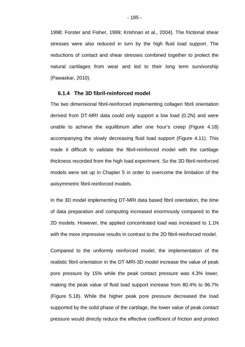
- 185 -
1998; Forster and Fisher, 1999; Krishnan et al., 2004). The frictional shear
stresses were also reduced in turn by the high fluid load support. The
reductions of contact and shear stresses combined together to protect the
natural cartilages from wear and led to their long term survivorship
(Pawaskar, 2010).
6.1.4 The 3D fibril-reinforced model
The two dimensional fibril-reinforced implementing collagen fibril orientation
derived from DT-MRI data could only support a low load (0.2N) and were
unable to achieve the equilibrium after one hour’s creep (Figure 4.18)
accompanying the slowly decreasing fluid load support (Figure 4.11). This
made it difficult to validate the fibril-reinforced model with the cartilage
thickness recorded from the high load experiment. So the 3D fibril-reinforced
models were set up in Chapter 5 in order to overcome the limitation of the
axisymmetric fibril-reinforced models.
In the 3D model implementing DT-MRI data based fibril orientation, the time
of data preparation and computing increased enormously compared to the
2D models. However, the applied concentrated load was increased to 1.1N
with the more impressive results in contrast to the 2D fibril-reinforced model.
Compared to the uniformly reinforced model, the implementation of the
realistic fibril orientation in the DT-MRI-3D model increase the value of peak
pore pressure by 15% while the peak contact pressure was 4.3% lower,
making the peak value of fluid load support increase from 80.4% to 96.7%
(Figure 5.18). While the higher peak pore pressure decreased the load
supported by the solid phase of the cartilage, the lower value of peak contact
pressure would directly reduce the effective coefficient of friction and protect

- 186 -
the cartilage. These results were extremely different from those in the 2D
fibril-reinforced model with realistic fibril orientation - the higher peak pore
pressure (Figures 4.9) was always accompanied by the higher peak contact
pressure (Figures 4.8) which would affect the function of the fluid load
support on protecting the cartilage. The reason leading to this difference
might be the slightly larger vertical deformation of the first cartilage layer in
the DT-MRI-3D model (Figure 5.23) - the oblique fibrils in this layer reduced
the stiffness compared to the Uniform-3D model. However, the first layer
deformed less in the 2D DT-MRI based model (Figures 4.13).
Another important finding of the 3D fibril-reinforced model implementing
realistic fibril orientation was that the load could be further increased to 5.4
N, which matched the 0.2 MPa pressure applied in the experiment of
unconfined compression (Section 5.4), and the 3D model was able to
achieve the equilibrium after one hour’s creep (Figure 5.26) making it
feasible to validate the model with the experimental data (Section 5.3).
The 3D model was validated by using the modelling result on cartilage
deformation to curve-fit the normalized experimental record of cartilage
thickness. The main factors that influenced the curve of vertical deformation
of cartilage in the 3D fibril-reinforced model were the Young’s modulus of the
nonfibrillar matrix Em and the permeability k. Through manually adjusting the
value of these two parameters, the curve of the 3D model with Em = 0.66
MPa and k = 3.0 × 10⁻¹⁵ m4/(N∙s) successfully achieved the same
equilibrium value as the experimental data with apparent deviation existing
from the start stage until the equilibrium of experiment (Figure 5.30). The
deviation could be reduced apparently by decreasing the permeability to k =
- 187 -
1.0 × 10⁻¹⁵ m4/(N∙s), although this made those two modelling curves unable
to achieve equilibrium in the experiment time (Figure 5.31). Actually, the
modelling results could curve-fit the experimental data best by adjusting
more parameters in the meantime (Lei et al., 2007). The procedure of Lei et
al. (2007) could estimate six parameters of the fibril-reinforced poroelastic
cartilage model in Li et al. (1999) and could be adapted to other models
under different experimental configuration. This would transfer the validation
of the 3D fibril-reinforced model to the problem of extracting material
parameters from the experimental data. However, the problem of material
parameter estimation was beyond the scope of the thesis and might be the
focus of work in the future.
6.1.5 Limitations
There were several limitations in the 3D fibril-reinforced model. The aspect
ratio along global Y-axis of the 3D elements was set to be 8:74 in order to
save the time of computing. This led to the irregular distribution of pore
pressure on the bottom of cartilage in the uniformly reinforced and the fibril-
reinforced models, without apparent influence to the isotropic model (Figure
5.16). However, it did not affect the pore pressure and fluid load support on
the cartilage surface (Figure 5.12-13 and 5.15).
As only one cross-section with 2mm thickness of the cartilage sample was
scanned, no information related to the orientation were derived for the fibrils
in the remaining region of the sample. The one same fibril orientation was
implemented to the eight elements which were defined as an element set in
the DT-MRI-3D model and made the model less realistic. This problem may
be solved by scanning several parallel slices of cartilage at different time,
- 188 -
with a less thickness such as 0.8 mm in Pierce et al. (2010) using a cuboids
sample. The increased slices of fibril orientation may also help to solve the
previous problem related to the aspect ratio: the mesh density along global
Y-axis can be increased with equal or less number of elements defined in
the same element set. Furthermore, to use cuboids cartilage sample in the
MRI scanning and compression test could solve the validation problem in
Section 5.4 where different kinds of geometry were used in experiment and
modelling.
For the validation of the 3D fibril-reinforced model, the experimental data
itself may be a factor to affect the curve-fitting - the method used to record
the thickness of the cartilage might underestimate the cartilage thickness
although the deformations were approximately correct (according to Dr
Robin Damion who performed the experiment).
In spite of these limitations, the implementation of “UMAT” (Dr L. P. Li,
University of Calgary) and “ORIENTATION” including “Distribution” made it
possible to investigate fluid load support in the 2D and 3D models reinforced
by collagen fibril, with strain dependent Young’s modulus and realistic fibril
orientation derived from DT-MRI data. The fibril reinforcement enhanced the
pressurization of the interstitial fluid and produced higher fluid load support
on the cartilage surface to protect the tissue from degradation by reducing
solid-to-solid contact.

- 189 -
6.2 The Conclusions
The major conclusions of this work were:
1) The peak value of fluid load support in both 2D and 3D fibril-
reinforced models was increased to greater than 80% from around
60% compared to the isotropic models, due to the reinforcement by
collagen fibril, regardless of whether that reinforcement was idealized
or derived from the DT-MRI data.
2) The 3D fibril-reinforced model implementing DT-MRI data did have
the capability to support the high load applied in the experiment. The
more important finding was that the cartilage could achieve
equilibrium, hence this model was validated by curve-fitting the
experimental record of cartilage thickness.
3) The implementation of the realistic fibril orientation derived from DT-
MRI data in the 3D fibril-reinforced model increase the value of peak
pore pressure by 15% compared to the uniformly reinforced model
while the peak contact pressure was 4.3% lower, making the peak
value of fluid load support increase from 80.4% to 96.7%.
4) The rationality to define the principal eigenvector as orientation of the
corresponding primary collagen fibril in the fibril-reinforced models
was verified by the positive results in 1), 2) and 3).
5) The feasibility and reliability of the methodologies to implement the
DT-MRI data to the fibril-reinforced models was both confirmed in the
process of validating the 3D model in 3).
- 190 -
6.3 Further Work
The main predictions of this study were the fluid load support on cartilage
surface and the distribution of the pore pressure and fluid flow throughout
the tissue. The reinforcement of collagen fibrils has been proved to enhance
the pressurization of the interstitial fluid and produced high pore pressure
within the cartilage, leading to the high fluid load support on the surface to
protect the cartilage against friction and wear.
The methodologies and models proposed in this study may be adapted to
investigate other experimental configurations such as indentation and
confined compression. The user subroutine “UMAT” in ABAQUS (Dr L. P. Li,
University of Calgary) had been successfully implemented to set up the
whole joint model (Gu and Li, 2010). The “ORIENTATION” needs much
more detailed DT-MRI information to define the orientation of collagen fibrils
throughout the whole natural cartilages. The high resolution MRI scanning is
difficult to perform on the whole joint and this might be the reason that Gu
and Li, (2010) used the split-line pattern rather than the DT-MRI method to
derive the fibril orientation of natural cartilages.
The material parameters and their values used in the fibril-reinforced models
were selected from Li et al. (2009) which were derived by manually curve-
fitting the experimental data (Li et al. 2003). So the value of each single
parameter can be automatically optimized by the procedure of Lei et al.
(2007) to make the modelling result curve-fit the experimental data best.
The cuboids form of cartilage sample should be used as Pierce et al. (2010),
instead of the cylinder one to make the geometry in the models same as that

- 191 -
in the experiment. If possible, the cartilage sample would be scanned on
parallel slices of at different time to provide more information to define the
orientation of collagen fibrils throughout the sample and make the fibril-
reinforced models more realistic.

- 192 -
List of References
Adam C., Eckstein F., Milz S., Putz R., 1998. The distribution of cartilage
thickness within the joints of the lower limb of elderly individuals. J Anat
193:203–214.
Akizuki S, Mow VC, Muller F, Pita JC, Howell DS, Manicourt DH., 1986.
Tensile properties of human knee joint cartilage. I. Influence of ionic
conditions, weight bearing, and fibrillation on the tensile modulus. J Orthop
Res 4(4):379–392.
Al Ali D., Graichen H., Faber S., Englmeier K.H., Reiser M., Eckstein F.,
2002. Quantitative cartilage imaging of the human hind foot: precision and
inter-subject variability. J Orthop Res 20: 249-256.
Almeida, E. S., Spilker, R. L.,1997.Mixed and penalty finite element models
for the nonlinear behavior of biphasic soft tissues in finite deformation: part I
alternate formulations. Comput. Methods Biomech. Biomed. Eng.1, 25–46.
Armstrong, C.G., Lai, W.M., Mow, V.C., 1984. An analysis of the unconfined
compression of articular cartilage. J. Biomech. Eng. 106, 165–173.
Ateshian, G.A., Lai,W.M., Zhu,W.B., Mow, V.C., 1994. An asymptotic
solution for the contact of two biphasic cartilage layers. J. Biomech. 27,
1347–1360.
Ateshian, G.A., Wang, H., 1995. A theoretical solution for the frictionless
rolling contact of cylindrical biphasic articular cartilage layers. J. Biomech.
28, 1341–1355.
Ateshian, G.A., 1997. A theoretical formulation for boundary friction in
articular cartilage. J. Biomech. Eng. 119, 81–86.
Ateshian, G.A.,Wang, H., Lai,W.M., 1998. The role of interstitial fluid
pressurization and surface porosities on the boundary friction of articular
cartilage. J. Tribol. 120, 241–248.
Ateshian, G.A., Mow, V.C., 2005. Lubrication and wear of diarthrodial joints.
In: Mow, V.C., Huiskes, R. (Eds.), Basic Orthopaedic Biomechanics &
Mechano- Biology. Lippincott Williams & Wilkins, Philadelphia, PA; London.
Ateshian, G.A., 2009. The role of interstitial fluid pressurization in articular
cartilage lubrication. J. Biomech. 42, 1163-1176.

- 193 -
Atkinson P, Haut RC., 1995. Subfracture insult to the human cadaver
patellofemoral joint produces occult injury. J Orthop Res 13:936–44.
Bader DL, Kempson GE, Egan J, Gilbey W, Barrett AJ., 1992. The effects of
selective matrix degradation on the short-term compressive properties of
adult human articular cartilage. Biochim Biophys Acta 1116(2):147–54.
Bear, Jacob, 1972. Dynamics of Fluids in Porous Media, Dover. — ISBN 0-
486-65675-6.
Biot, M.A., 1941. General theory of three-dimensional consolidation. Journal
of Applied Physics 12, 155-164.
Buckwalter JA, Hunziker EB, Rosenberg LC, Coutts R, Adams M, Eyre D.,
1991. Articular cartilage: composition and structure. In: Wo SI, Buckwalter
JA, editors. Injury and repair of musculoskeletal soft tissues. 2nd ed. Park
Ridge: American Academy of Orthopaedic Surgeons, 405–25.
Bursac, P. M., Obitz, T. W., Eisenberg, S. R., and Stamenovic, D., 1999.
‘‘Confined and Unconfined Stress Relaxation of Cartilage: Appropriateness
of a Transversely Isotropic Analysis,’’ J. Biomech., 32, 1125–1130.
Callaghan P. Principles of Nuclear Magnetic Resonance Microscopy.
Oxford: Clarendon Press 1991.
Charnley, J., 1960. The lubrication of animal joints in relation to surgical
reconstruction by arthroplasty. Ann. Rheum. Dis. 19, 10–19.
Chegini, S., Ferguson, S.J., 2010. Time and depth dependent poisson’s ratio
of cartilage explained by an inhomogeneous orthotropic fiber embedded
biphasic model. Journal of Biomechanics, doi: 10. 1016/j. jbiomech. 2010.
03. 006
Chen, A.C., Bae, W.C., Schinagl, R.M., Sah, R.L., 2001. Depth- and strain-
dependent mechanical and electromechanical properties of full-thickness
bovine articular cartilage in confined compression. J. Biomech. 34, 1–12.
Cicuttini F, Forbes A, Morris K, Darling S, Bailey M, Stuckey S, 1999.
Gender differences in knee cartilage volume as measured by magnetic
resonance imaging. Osteoarthritis Cartilage 7, 265-271.
Cicuttini F, Forbes A, Asbeutah A, Morris K, Stuckey S, 2000. Comparison
and reproducibility of fast and conventional spoiled gradient-echo magnetic
resonance sequences in the determination of knee cartilage volume. J
Orthop Res; 18, 580-584.

- 194 -
Clark JM., 1991. Variation of collagen fiber alignment in a joint surface: a
scanning electron microscope study of the tibial plateau in dog, rabbit, and
man. J Orthop Res 9: 246–57.
Clarke IC., 1971. Articular cartilage: a review and scanning electron
microscope study. 1. The interterritorial fibrillar architecture. J Bone Joint
Surg Br 53:732–50.
Cohen, B., Gardner, T.R., Ateshian, G.A., 1993. The influence of transverse
isotropy on cartilage indentation behavior: A study of the human humeral
head. In: Transactions Orthopaedic Research Society. Orthopaedic
Research Society, Chicago, IL: 185.
Cohen, B., Lai, M.W., Mow, V.C., 1998. A transversely isotropic biphasic
model for unconfined compression of growth plate and chondroepophysis.
Journal of Biomechanical Engineering 120 (4): 491-496.
Cohen ZA, McCarthy DM, Kwak SD, Legrand P, Fogarasi F, Ciaccio EJ,
1999. Knee cartilage topography, thickness, and contact areas from MRI: in-
vitro calibration and in-vivo measurements. Osteoarthritis Cartilage 7: 95-
109
Cremer MA, Rosloniec EF, Kang AH., 1998. The cartilage collagens: a
review of their structure, organization, and role in the pathogenesis of
experimental arthritis in animals and in human rheumatic disease. J Mol Med
76:275–88.
DiSilvestro M.R., Zhu Q., Wong M., Jurvelin JS, Suh JK., 2001. Biphasic
poroviscoelastic simulation of the unconfined compression of articular
cartilage. I. Simultaneous prediction of reaction force and lateral
displacement. J Biomech Eng 123(2):191–7.
Dowson, D., Wright,V., Longfield, M.D., 1969. Human joint lubrication.
Biomed. Eng. 4,160–165.
Dowson D., 1990. Biotribology of natural and replacement synovial joints. In:
Mow VC, Ratcliffe A, Woo SLY, editors. Biomechanics of diarthroidal joints.
New York: Springer–Verlag; 305–45.
Eckstein F., Lemberger B., Gratzke C., Hudelmaier M., Glaser C., Englmeier
K.H., Reiser M., 2005. In vivo cartilage deformation after different types of
activity and its dependence on physical training status. Annals of the
Rheumatic Diseases 64 (2): 291–295.

- 195 -
Eckstein F, Sittek H, Schulte E, Kiefer B, Reiser M, Putz R. The potential of
magnetic resonance imaging (MRI) for quantifying articular cartilage
thickness - a methodological study. Clin Biomech 1995;10: 434-40.
Ethier CR, Simmons CA, 2007. Introductory biomechanics: from cells to
organisms. Cambridge, UK: Cambridge University Press.
Eyre DR, Apones S, Wu JJ, Ericksson LH, Walsh KA., 1987. Collagen type
IX: evidence for covalent linkages to type II collagen in cartilage. FEBS Lett
220:337–341.
Eyre DR., 1991. The collagens of articular cartilage. Sem Arthritis Rheum
21:2–11.
Federico, S., La Rosa, G., Herzog, W. and Wu, J.Z. , 2004. Effect of fluid
boundary conditions on joint contact mechanics and applications to the
modeling of osteoarthritic joints. Journal of Biomechanical Engineering.
126(2): 220-225.
Federico S., Grillo A., Rosa G.L., Giaquinta G., Herzog W., 2005. A
transversely isotropic, transversely homogeneous microstructure-statistical
model of articular cartilage. J Biomech 38: 2008 - 2018.
Forster, H., Fisher, J., 1996. The influence of loading time and lubricant on
the friction of articular cartilage. Proc. Inst. Mech. Eng. [H] 210, 109–119.
Forster, H., Fisher, J., 1999. The influence of continuous sliding and
subsequent surface wear on the friction of articular cartilage. Proc. Inst.
Mech. Eng. [H] 213, 329–345
Frank, E.H., Grodzinsky, A.J., 1987. Cartilage electromechanics II — a
continuum model of cartilage electrokinetics and correlation with
experiments. Journal of Biomechanics 20 (6), 629–639.
Fung Y.C., 1993. Biomechanics: Mechanical Properties of Living Tissues,
2nd edition. Springer-Verlag, New York.
Fermor, H.L., McLure, S. W.D., Taylor, S.D., Russell, S.L., Williams, S.,
Fisher, J. and Ingham, E., 2013. Biological biochemical and biomechanical
characterisation of articular cartilage from the porcine, bovine and ovine hip.
Biomedicine engineering and material. In process.
Garcia JJ, Aliero NJ, Haut RC., 1998. An approach for stress analysis of
transversely isotropic biphasic cartilage under impact load. J Biomech Eng
120:608–13.

- 196 -
Greene GW., Zappone B, So¨derman O, Topgaard D, Rata G, Hongbo Z,
Israelachvili JN, 2010. Anisotropic dynamic changes in the pore network
structure, fluid diffusion and fluid flow in articular cartilage under
compression. Biomaterials 31: 3117-3128.
Gu K.B., Li L.P., 2011. A human knee joint model considering fluid pressure
and fiber orientation in cartilages and menisci. Med Eng Phys 33:497–503.
Gu WY, Lai WM, Mow VC., 1993; Transport of fluid and ions through a
porous-permeable charged-hydrated tissue, and streaming potential data on
normal bovine articular cartilage. J Biomech 26:709–23.
Gu WY, Lai WM, Mow VC., 1998. A mixture theory for chargedhydrated soft
tissues containing multi-electrolytes: passive transport and swelling
behaviors. J Biomech Eng 120:169–80.
Guide for verification and validation in computational solid dynamics, 2006
(American Society of Mechanical Engineers, New York).
Gupta S., Lin J., Ashby P., Pruitt L.,2009. A fiber reinforced poroelastic
model of nanoindentation of porcine costal cartilage: A combined
experimental and finite element approach. J Mech. Beh. Biomed. Mater. 2:
326-338.
Hasler EM, Herzog W, Wu JZ, Muller W, Wyss U., 1999. Articular cartilage
biomechanics: theoretical models, material properties, and biosynthesis
response. Clin Rev Biomech Eng 27:415–88.
Hayes WC, Bodine AJ., 1978. Flow-independent viscoelastic properties of
articular cartilage matrix. J Biomech 11(8–9):407– 19.
Higginson GR, Litchfield MR, Snaith J, 1976. Load–displacement – time
characteristics of articular cartilage. Int J Mech Sci 18:481–486
Hunter W., 1743. Of the Structure and Disease of Articulating Cartilage, Phi,
Trans. Roy., Vol. 42, 514.
Holmes M.H. and Mow V.C., 1990. The nonlinear characteristics of soft gels
and hydrated connective tissues in ultra-filtration. J Biomech 23: 1145 -
1156.
Hunziker EB, Michel M, Studer D., 1997. Ultrastructure of adult human
cartilage matrix after cryotechnical processing. Microsc Res Technol
37:271–84.
Huyghe J.M., Janssen J.D. 1997. Quadriphasic mechanics of swelling
incompressible porous media. Int. J. Eng. Sci. 35, 793–802.

- 197 -
Huyghe JM, Janssen CF, Van Donkelaar CC, Lanir Y., 2002. Measuring
principles of frictional coefficients in cartilaginous tissues and its substitutes.
Biorheology. 39, 47–53.
Jay, G.D., Tantravahi, U., Britt, D.E., Barrach, H.J., Cha, C.J., 2001.
Homology of lubricin and superficial zone protein (SZP): products of
megakaryocyte stimulating factor (MSF) gene expression by human synovial
fibroblasts and articular chondrocytes localized to chromosome 1q25. J.
Orthop. Res. 19, 677–687.
Julkunen P, Kiviranta P, Wilson W, Jurvelin JS, Korhonen RK, 2007.
Characterization of articular cartilage by combining microscopic analysis with
a fibril-reinforced finite-element model. J Biomech 40:1862–1870.
Julkunen, P., R. K. Korhonen, W. Herzog, and J. S. Jurvelin., 2008a.
Uncertainties in indentation testing of articular cartilage: a fibril-reinforced
poroviscoelastic study. Med. Eng. Phys. 30:506–515.
Julkunen P, Korhonen RK, Nissi MJ, Jurvelin JS, 2008b. Mechanical
characterization of articular cartilage by combining magnetic resonance
imaging and finite-element analysis: a potential functional imaging
technique. Phys Med Biol 53: 2425–2438.
Julkunen p., Jurvelin J.S., Isaksson H., 2010. Contribution of tissue
composition and structure to mechanical response of articular cartilage
under different loading geometries and strain rates. Biomech Model
Mechanobiol 9: 237-245.
Junqueira LC, Carneiro J., 1983. Basic histology. 4th ed. Los Altos: Lange
Medical; 129.
Kaab, M. J.; Gwynn, I. A. P.; Notzli, H. P., 1998: Collagen fibre arrangement
in the tibial plateau articular cartilage of man and other mammalian species.
Journal Of Anatomy. 1: 23-34, Y 193: 23-34.
Katta J., Pawaskar S.S., Jin, Z., Ingham E., Fisher J., 2007. Effect of load
variation on the friction properties of articular cartilage. Proc. Instn Mech
Engrs 221 Part J: J. Engineering Tribology 175 – 181.
Katta, J., Jin, Z., Ingham, E., Fisher, J., 2008. Biotribology of articular
cartilage — a review of the recent advances. Med. Eng. Phys. 30, 1349–
1363.

- 198 -
Kazemi M., Dabiri Y., and Li L. P., 2013. Recent Advances in Computational
Mechanics of the Human Knee Joint. Computational and Mathematical
Methods in Medicinehttp://dx.doi.org/10.1155/2013/718423.
Kiviranta P, Rieppo J, Korhonen RK, Julkunen P, Töyräs J, Jurvelin JS,
2006. Collagen network primarily controls poisson’s ratio of bovine articular
cartilage in compression. J Orthop Res 24:690– 699
Korhonen, R.K., Laasanen, M.S., Toyras, J., Lappalainen, R., Helminen,
H.J., Jurvelin, J.S., 2003. Fibril reinforced poroelastic model predicts
specifically mechanical behavior of normal, proteoglycan depleted and
collagen degraded articular cartilage. J Biomech 36: 1373–1379.
Krishnan, R., Caligaris, M., Mauck, R.L., Hung, C.T., Costa, K.D., Ateshian,
G.A., 2004a. Removal of the superficial zone of bovine articular cartilage
does not increase its frictional coefficient. Osteoarthritis Cartilage 12, 947–
955.
Krishnan, R., Kopacz, M., Ateshian, G.A., 2004. Experimental verification of
the role of interstitial fluid pressurization in cartilage lubrication. J. Orthop.
Res. 22, 565–570.
Krishnan, R., Mariner, E.N., Ateshian, G.A., 2005. Effect of dynamic loading
on the frictional response of bovine articular cartilage. J. Biomech. 38, 1665–
1673.
Larry W Moreland, 2003. Intra-articular hyaluronan (hyaluronic acid) and
hylans for the treatment of osteoarthritis: mechanisms of action. Arthritis Res
5(2): 54–67.
L. P. Rasanen, M. E. Mononen, M. T. Nieminen, E. Lammentausta, J. S.
Jurvelin, and R. K. Korhonen, 2012. Implementation of subject-specific
collagen architecture of cartilage into a 2D computational model of a knee
joint—data from the Osteoarthritis Initiative (OAI),” Journal of Orthopaedic
Research, vol. 31, no. 1, 10–22.
Lai WM., Mow VC., Roth V., 1981. Effects of nonlinear strain-dependent
permeability and rate of compression on the stress behavior of articular
cartilage. J Biomech Eng; 103: 61–66.
Le Bihan D, Mangin J-F, Poupon C, Clark CA, Pappata S, Molko N, et al.
2001. Diffusion tensor imaging: concepts and applications. J Magn Reson
Imaging. 13:534-46.
- 199 -
Lei F. and Szeri A.Z., 2007. Inverse analysis of constitutive models:
Biological soft tisues. J Biomech 40: 936 - 940.
Lewis, P.R., McCutchen, C.W., 1959. Experimental evidence for weeping
lubrication in mammalian joints. Nature 184, 1285.
Li, L.P., Soulhat J., Buschmann M.D., Shirazi-Adl A., 1999. Nonlinear
analysis of cartilage in unconfined ramp compression using a fibril reinforced
poroelastic model. Clin. Biomech. 14(9), 673–682.
Li, L.P., Buschmann MD, Shirazi-Adl A., 2000. A fibril reinforced
nonhomogeneous poroelastic model for articular cartilage: inhomogeneous
response in unconfined compression. J Biomech. 33(12), 1533–1541.
Li, L.P., Buschmann MD, Shirazi-Adl A., 2001. The asymmetry of transient
response in compression versus release for cartilage in unconfined
compression. J. Biomech. Eng. 123, 519–522.
Li, L.P., Shirazi-Adl A, Buschmann MD., 2002. Alterations in mechanical
behaviour of articular cartilage due to changes in depth varying material
properties—a nonhomogeneous poroelastic model study. Comput. Meth.
Biomech. Biomed. Eng. 5(1), 45–52.
Li, L.P., Buschmann MD, Shirazi-Adl A., 2003. Strain-rate dependent
stiffness of articular cartilage in unconfined compression. J. Biomech
Eng.125(2), 161–168.
Li L.P., Herzog W., 2004. The role of viscoelasticity of collagen fibers in
articular cartilage: theory and numerical formulation. Biorheology 41:181–
194.
Li L.P., J. T. M. Cheung, Herzog W., 2009. Three-dimensional fibril-
reinforced finite element model of articular cartilage. Medical & Biological
Engineering & Computing 47(6): 607-615.
Macirowski, T., Tepic, S., Mann, R.W., 1994. Cartilage stresses in the
human hip joint. J. Biomech. Eng. 116, 10–18.
Mak A.F., 1986. The apparent viscoelastic behavior of articular cartilage —
the contributions from the intrinsic matrix viscoelasticity and interstitial fluid
flows. J Biomech Eng 108(2):123–30.
Mak A.F, Lai WM, Mow VC., 1987. Biphasic indentation of articular cartilage.
I. Theoretical analysis. J Biomech 20(7):703–14.

- 200 -
Mak A.F., 1986. The apparent viscoelastic behavior of articular cartilage —
the contributions from the intrinsic matrix viscoelasticity and interstitial fluid
flows. J Biomech Eng 108(2):123–30.
Maroudas A., 1968. Physicochemical properties of cartilage in the light of
ion-exchange theory. Biophys J 8:575–595
Maroudas A., 1975. Biophysical chemistry of cartilaginous tissues with
special reference to solute and fluid transport. Biorheology 12:233–48.
Maroudas A., 1976. Balance between swelling pressure and collagen
tension in normal and degenerate cartilage. Nature 260, 808–809.
Maroudas A., 1979. Physicochemical properties of articular cartilage. In:
Freeman MAR, editor. Adult articular cartilage. 2nd ed. Kent, UK: Pitman
Med.; 215–323.
McCutchen, C.W., 1962. The frictional properties of animal joints. Wear 5,
1–17.
McCutchen, C.W., 1966. Boundary lubrication by synovial fluid:
demonstration and possible osmotic explanation. Fed. Proc. 25, 1061.
McCutchen, C.W., 1983. Joint lubrication. Bull. Hosp. Jt. Dis. Orthop. Inst.
43, 118–129.
McGibbon CA, Bencardino J, Yeh ED, Palmer WE, 2003. Accuracy of
cartilage and subchondral bone spatial thickness distribution from MRI. J
Magn Reson Imag 17:703-15.
Meder R, de Visser SK, Bowden JC, Bostrom T, Pope JM. Diffusion tensor
imaging of articular cartilage as a measure of tissue microstructure.
Osteoarthritis Cartilage 2006;14:875-81.
Mente PL, Lewis JL., 1994. Elastic modulus of calcified cartilage is an order
of magnitude less than that of subchondral bone. J Orthop Res 12:637–47.
Michal Kozanek, Ali Hosseini, Fang Liu, Samuel K.Van de Velde, Thomas J.
Gill, Harry E, Rubash, Guoan Li, 2009. Tibiofemoral kinematics and condylar
motion during the stance phase of gait. J. Biomech. 42(12): 1877-1884.
Mononen M.E., Julkunen P., Töyräs J., Jurvelin J.S., Kiviranta I., Korhonen
R.K. 2010. Alterations in structure and properties of collagen network of
osteoarthritic and repaired cartilage modify knee joint stresses. Biomech
Model Mechanobiol DOI 10.1007/s10237-010-0239-1.
- 201 -
Morgan FR., 1960. Mechanical properties of collagen and leather fibres. Am
Leather Chem Assoc J., 55(1): 23–24.
Mow, V.C., Kuei, S.C., Lai, W.M., Armstrong, C.G., 1980. Biphasic creep
and stress relaxation of articular cartilage: theory and experiment. ASME
Journal of Biomechanical Engineering 102: 73-84.
Mow VC, Holmes MH, Lai WM., 1984. Fluid transport and mechanical
properties of articular cartilage: a review. J Biomech 17(5):377–94.
Mow VC, Proctor CS, Kelly MA., 1989. Biomechanics of articular cartilage.
In: Nordin M, Frankel VH, editors. Basic biomechanics of the mucoskeletal
system. 2nd ed. Philadelphia, PA: Lea and Febiger; 31–57.
Mow VC, Zhu W, Ratclife A., 1991. Structure and function of articular
cartilage and meniscus. In: Mow VC, Hayes WC, editors. Basic orthopaedic
biomechanics. New York: Raven Press; 143–198.
Mow VC, Ratcliffe A, Poole AR., 1992. Cartilage and diarthrodial joints as
paradigms for hierarchical materials and structures. Biomaterials 13:67–97.
Mow, V.C., Ratcliffe, A., 1997. Structure and function of articular cartilage
and meniscus. In: Mow, V.C., Hayes, W.C. (Eds.), Basic Orthopaedic
Biomechanics. Lippincott-Raven, Philadelphia p. xiii, 514.
Mow VC, Guo XE., 2002. Mechano-electrochemical properties of articular
cartilage: their inhomogeneities and anisotropies. Annu Rev Biomed Eng
4:175–209.
Oloyede, A., Broom, N.D., 1994. The generalized consolidation of articular
cartilage: an investigation of its near-physiological response to static load.
Connective Tissue Research 31 (1), 75–86.
Oloyede, A., Broom, N.D., 1991. Is classical consolidation theory applicable
to articular cartilage deformation? Clin. Biomech. (Bristol, Avon) 6, 206–212.
Oegema Jr TR, Carpenter RJ, Hofmeister F, Thompson Jr RC., 1997. The
interaction of the zone of calcified cartilage and subchondral bone in
osteoarthritis. Microsc Res Technol 37:324–32.
Park, S., Krishnan, R., Nicoll, S.B., Ateshian, G.A., 2003. Cartilage interstitial
fluid load support in unconfined compression. J. Biomech. 36, 1785–1796.
Pawaskar SS, Fisher J, Jin Z. 2010. Robust and general method for
determining surface fluid flow boundary conditions in articular cartilage
contact mechanics modeling. Journal of Biomechanical Engineering 132(3),
1- 8.

- 202 -
Pierce, D. M., Ricken T., and G. A. Holzapfel., 2012. Modeling
Sample/Patient-Specific Structural and Diffusional Response of Cartilage
Employing DT-MRI. Int. J. Numer. Meth. Biomed. Engng. 2012; 00:1–15.
Pierce D. M., Trobin W.,RAYA J. G., Tratting S., Bischof H., Glaser C., and
Holzapfel G. A., 2010. DT-MRI based computation of collagen fiber
deformation in human articular cartilage: A feasibility study. Annuals of
Biomedical Engineering. 38 (7): 2447-2463.
Puso M.A. and Weiss J.A., 1998. Finite element implementation of
anisotropic quasi-linear viscoelasticity using a discrete spectrum
approximation, ASME J. Biomechanical Eng. 120, 62–70.
Quinn TM, Kocian P, Meister JJ., 2000. Static compression is associated
with decreased diffusivity of dextrans in cartilage explants. Arch. Biochem.
Biophys. 384(2), 327–34.
Quinn, TM, Morel V. , 2007 Microstructural modeling of collagen network
mechanics and interactions with the proteoglycan gel in articular cartilage.
Biomech. Model. Mechanobiol. 6:73–82.
Quiñonez, A.F., Summers, J.L., Fisher, J., Jin, Z.M., 2010. An analytical
solution for the radial and tangential displacements on a thin hemispherical
layer of articular cartilage. Biomech. Model. Mechanobiol. Volume 10, Issue
3, 283-293.
Radin, E.L., Swann, D.A., Weisser, P.A., 1970. Separation of a hyaluronate-
free lubricating fraction from synovial fluid. Nature 228, 377–378.
Reynaud B, Quinn TM, 2006. Anisotropic hydraulic permeability in
compressed articular cartilage. J Biomech 39:131–137
Roth V, Mow VC., 1980. The intrinsic tensile behavior of the matrix of bovine
articular cartilage and its variation with age. J Bone Joint Surg Am 62:1102–
17.
Sainath Shrikant Pawaskar, 2006. Contact Mechanics Modelling of Articular
Cartilage and Applications. Master thesis, University of leeds.
Sainath Shrikant Pawaskar, 2010. PhD thesis, University of leeds.
Sanjeevi R, Somanathan N, Ramaswamy D., 1982. A viscoelastic model for
collagen fibres. J Biomech 15:181–3.

- 203 -
Schmidt, T.A., Gastelum, N.S., Nguyen, Q.T., Schumacher, B.L., Sah, R.L.,
2007. Boundary lubrication of articular cartilage: role of synovial fluid
constituents. Arthritis Rheum. 56, 882–891.
Setton LA, Zhu WB, Mow VC, 1993. The biphasic poroviscoelastic behavior
of articular cartilage: role of the surface zone in governing the compressive
behavior. J Biomech 26:581–592
Shirazi R., Shirazi-Adl A., 2005. Analysis of articular cartilage as a
composite using nonlinear membrane elements for collagen fibrils. Medical
Engineering & Physics 27: 827–835.
Shirazi R., Shirazi-Adl A., 2008. Deep Vertical Collagen Fibrils Play a
Significant Role in Mechanics of Articular Cartilage. JOURNAL OF
ORTHOPAEDIC RESEARCH 23: 608-615.
Silyn-Roberts H, Broom ND., 1990. Fracture behaviour of cartilage-on-bone
in response to repeated impact loading. Connect Tiss Res 24:143–56.
Simon, B.R., 1992. Multiphasic poroelastic finite element models for soft
tissue structures. Applied Mechanics Reviews 45: 191-218.
Soltz, M.A., Ateshian, G.A., 1998. Experimental verification and theoretical
prediction of cartilage interstitial fluid pressurization at an impermeable
contact interface in confined compression. J. Biomech. 31: 927–934.
Soltz, M.A., Ateshian, G.A., 2000a. Interstitial fluid pressurization during
confined compression cyclical loading of articular cartilage. Ann. Biomed.
Eng. 28: 150–159.
Soltz, M.A., Ateshian, G.A., 2000b. A conewise linear elasticity mixture
model for the analysis of tension–compression nonlinearity in articular
cartilage. J. Biomech. Eng. 122, 576–586.
Soltz, M.A., Basalo, I.M., Ateshian, G.A., 2003. Hydrostatic pressurization
and depletion of trapped lubricant pool during creep contact of a rippled
indenter against a biphasic articular cartilage layer. J. Biomech. Eng. 125:
585–593.
Soulhat J, Buschmann MD, Shirazi-Adl A. 1999. A fibril-network reinforced
biphasic model of cartilage in unconfined compression. J. Biomech Eng.
121(3): 340–347.
Spilker, R.L., Suh, J.K., 1990. Formulation and evaluation of a finite element
model for the biphasic model of hydrated soft tissues. Comput. Struct. 35:
425–439.

- 204 -
Spilker, R.L., Suh, J.K. and Mow, V.C., 1992. A finite-element analysis of the
indentation stress-relaxation response of linear biphasic articular-cartilage.
Journal of Biomechanical Engineering-Transactions of the ASME, 114(2): p.
191-201.
Stewart,T.D. , Hall, R.M. , 2006. Basic biomechanics of human joints: Hips,
knees and the spine. Current Orthopaedics, 20(1) 23-31.
Stockwell RA., 1979. Biology of cartilage cells. Cambridge: Cambridge
University Press.
Suh, J. K., Spilker, R.L., Holmes, M.H., 1991. A penalty finite element
analysis for nonlinear mechanics of biphasic hydrated soft tissue under large
deformation. Int. J. Numer. Methods Eng. 32: 1411–1439.
Suh, J. K., DiSilvestro, M. R., 1997, ‘‘Biphasic Poroviscoelastic Theory of
Articular Cartilage: Experimental Validation Through Unconfined
Compression,’’ Proc. ASME Summer Bioengineering Conference, Vol. 35:
31–32.
Suh, J. K., Bai, S., 1997, ‘‘Biphasic Poroviscoelastic Behavior of Articular
Cartilage in Creep Indentation Test,’’ Proc. 43rd Annual Meeting of the
Orthopaedic Research Society, Vol. 22: 823.
Suh J.K., Bai S., 1998. Finite element formulation of biphasic
poroviscoelastic model for articular cartilage. J Biomech Eng 120(2): 195–
201.
Swann, D.A., Radin, E.L., 1972. The molecular basis of articular lubrication.
I. Purification and properties of a lubricating fraction from bovine synovial
fluid. J. Biol. Chem. 247, 8069–8073.
Taylor Z. A. and Miller K., 2006. Constitutive modeling of cartilaginous
tissues: a review. Journal of Biomechanics, vol. 22, no. 3, pp. 212–229.
Thomas M.Q., Ernst B.H. and Hans-Jorg H., 2005. Variation of cell and
matrix morphologies in articular cartilage among locations in the adult
human knee. OsteoArthritis and Cartilage 13, 672-678.
Urban JPG, Maroudas A, Bayliss MT, Dillon J., 1979. Swelling pressures of
PG’s at the concentrations found in cartilagenous tissues. Biorheology
16:447–464.
Visser S.K., Crawford R.W., Pope J.M., 2008. Structural adaptations in
compressed articular cartilage measured by diffusion tensor imaging.
Osteoarthritis Cartilage. 16, 83-89.

- 205 -
Visser SK, Bowden JC, Wentrup-Bryne E, Rintoul L, Bostrom T, Pope JM,
Momot KI. Anisotropy of collagen fibre alignment in bovine cartilage:
comparison of polarised light microscopy and spatially resolved diffusion-
tensor measurements. Osteoarthritis Cartilage 2008 (b); 16:689-697.
Viidik, A., 1968. A Rheological Model for Uncalcified Parallel-Fibered
Collagenous Tissues. J. Biomech., 1: 3–11.
Walker, P.S., Dowson, D., Longfield, M.D., Wright, V., 1968. ‘‘Boosted
lubrication’’ in synovial joints by fluid entrapment and enrichment. Ann.
Rheum. Dis. 27: 512–520.
Wang CC, Hung CT, Mow VC., 2001. An analysis of the effects of depth-
dependent aggregate modulus on articular cartilage stress-relaxation
behavior in compression. J Biomech 34(1):75–84.
Warner, M.D. Finite element biphasic modelling of articular cartilage: aninvestigation into crystal induced damage. Ph D Thesis. 2000, University ofBath. 177.
Warner, M.D., Taylor, W.R., et al., 2001a. Finite element biphasic
indentation of cartilage: A comparison of experimental indenter and
physiological contact geometries. Proceedings of the Institution of
Mechanical Engineers Part HJ Eng. Med. 215 (H5), 48-496.
Warner, M.D., Taylor,W.R., et al., 2001b. A method for determining contact
between a nonporous surface and articular cartilage in a biphasic FE
model. In: Middleton, J., Jones, M.L., Pande, G. (Eds.), Computer Methods
in Biomechanics and Bioengineering 3. Gordon and Breach Science
Publishers, pp. 207.212.
Wayne, J.S., Woo, S.L., Kwan, M.K., 1991. Application of the u-p finite
element method to the study of articular cartilage. J. Biomech. Eng. 113:
397–403.
Wilson W., van Donkelaar CC., van Rietbergen C., Ito K., Huiskes R.,2004.
Stresses in the local collagen network of articular cartilage: a
poroviscoelastic fibril-reinforced finite element study. J. Biomech. 37(3):
357–366.
Wilson W., van Donkelaar CC., van Rietbergen R., Huiskes R., 2005a. A
fibril-reinforced poroviscoelastic swelling model for articular cartilage. J
Biomech. 38, Issue 6: 1195-1204.
Wilson W., van Donkelaar CC., van Rietbergen R., Huiskes R., 2005b. The
role of computational models in the search for the mechanical behavior and
- 206 -
damage mechanisms of articular cartilage. Medical Engineering & Physics,
27: 810-826.
Wilson W, Huyghe JM, van Donkelaar CC, 2006. A composition-based
cartilage model for the assessment of compositional changes during
cartilage damage and adaptation. Osteoarthritis Cartilage 14: 554–560.
Wilson W, Huyghe JM, van Donkelaar CC, 2007. Depth-dependent
compressive equilibrium properties of articular cartilage. Biomech Model
Mechanobiol 6: 43–53.
Wong M, Wuethrich P, Eggli P, Hunziker EB., 1996, Zone-specific cell
biosynthesis activity in mature bovine articular cartilage: a new method using
confocal microscopic stereology and quantitative autoradiography. J Orthop
Res 14: 424–432.
Wong M, Wuethrich P, Buschmann MD, Eggli P, Hunziker EB., 1997.
Chondrocyte biosynthesis correlates with local tissue strain in statically
compressed adult articular cartilage. J Orthop Res 15:189–96.
Wu, J. Z., Herzog, W., Epstein, M., 1998. Evaluation of the finite element
software ABAQUS for biomechanical modelling of biphasic tissues. J.
Biomech. 31: 165–169.

- 207 -
Appendix A List of Publications
Conference Abstract:
1) An, Shuqiang; Jones Alison; Damion Robin; Fisher John and Jin
Zhongmin. Realistic Fibril Distribution Basing on DT-MRI Data Enhances
Pressurization of Interstitial Fluid in 2D Fibril-Reinforced Cartilage Model.
Podium presentation. Paper No. 0396, Session 66. Annual Meeting of the
Orthopaedic Research Society, 2013, San Antonio, Texas.

- 208 -
Appendix B Derivation of the Contribution of Fibillar Matrix
According to Section 3.2.2, the fibrillar stress in the iterative step (t + ઢt) was
calculated as:
௫ߪ(ݐ+ (ݐ߂ = ௫ߪ
(0) + න ௫ܩ
௧ା௱௧
+ݐ) −ݐ߂ ௫ܧ((ߝ௫ ௫ߝ( (B. 1)
Splitting the integration followed by a series of equivalent conversion,
formula (B.1) was rewritten as:
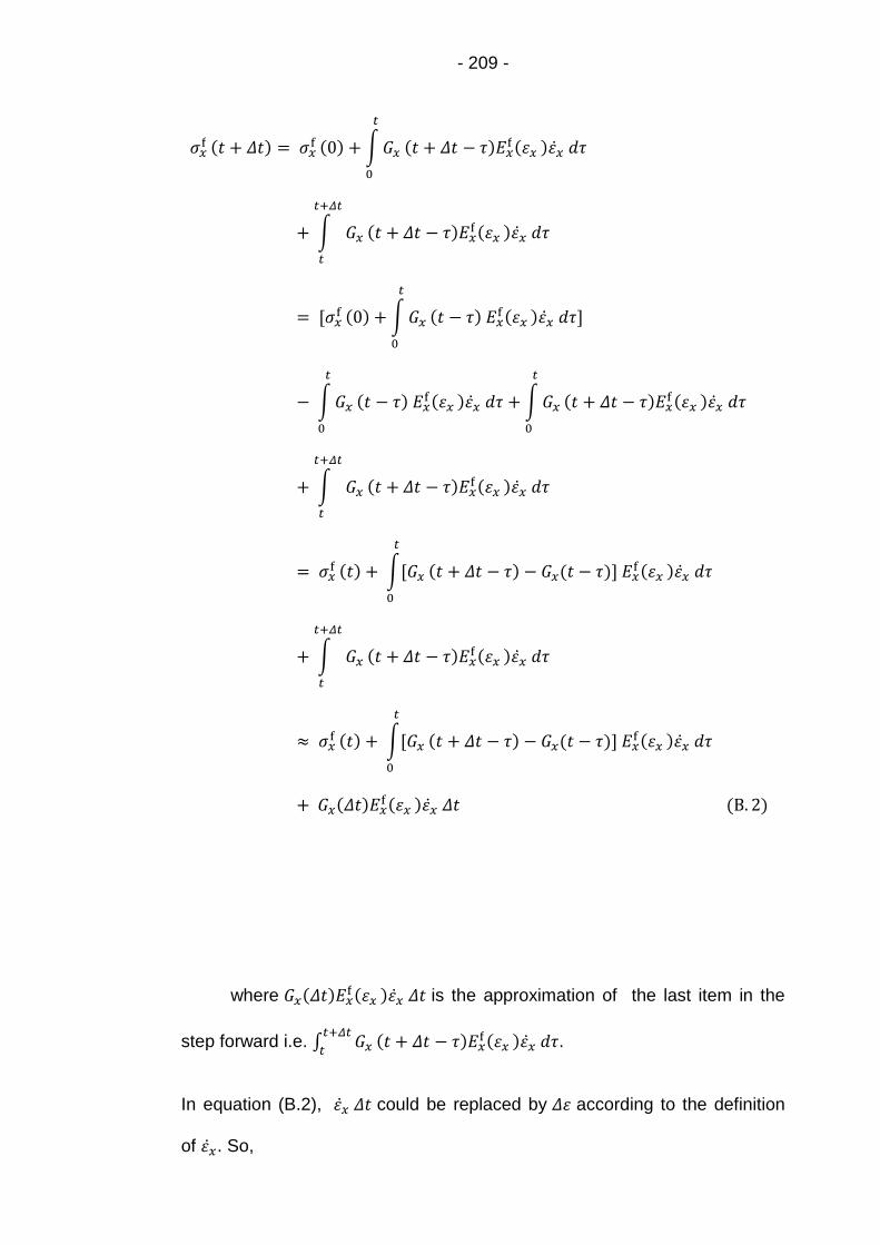
- 209 -
௫ߪ(ݐ+ (ݐ߂ = ௫ߪ
(0) + න ௫ܩ
௧
+ݐ) −ݐ߂ ௫ܧ((ߝ௫ ௫ߝ(
+ න ௫ܩ
௧ା௱௧
௧
+ݐ) −ݐ߂ ௫ܧ((ߝ௫ ௫ߝ(
= ௫ߪ](0) + න ௫ܩ
௧
−ݐ) ) ௫ܧ(ߝ௫ ௫ߝ( ]
− න ௫ܩ
௧
−ݐ) ) ௫ܧ(ߝ௫ ௫ߝ( + න ௫ܩ
௧
+ݐ) −ݐ߂ ௫ܧ((ߝ௫ ௫ߝ(
+ න ௫ܩ
௧ା௱௧
௧
+ݐ) −ݐ߂ ௫ܧ((ߝ௫ ௫ߝ(
= ௫ߪ(ݐ) + න ௫ܩ]
௧
+ݐ) −ݐ߂ ) − −ݐ)௫ܩ )] ௫ܧ(ߝ௫ ௫ߝ(
+ න ௫ܩ
௧ା௱௧
௧
+ݐ) −ݐ߂ ௫ܧ((ߝ௫ ௫ߝ(
≈ ௫ߪ(ݐ) + න ௫ܩ]
௧
+ݐ) −ݐ߂ ) − −ݐ)௫ܩ )] ௫ܧ(ߝ௫ ௫ߝ(
+ ௫ܧ(ݐ߂)௫ܩ(ߝ௫ ௫ߝ( ݐ߂ (B. 2)
where ௫ܧ(ݐ߂)௫ܩ(ߝ௫ ௫ߝ( isݐ߂ the approximation of the last item in the
step forward i.e. ∫ ௫ܩ௧ା௱௧
௧+ݐ) −ݐ߂ ௫ܧ(
(ߝ௫ ௫ߝ( .
In equation (B.2), ௫ߝ couldݐ߂ be replaced by accordingߝ߂ to the definition
of .௫ߝ So,
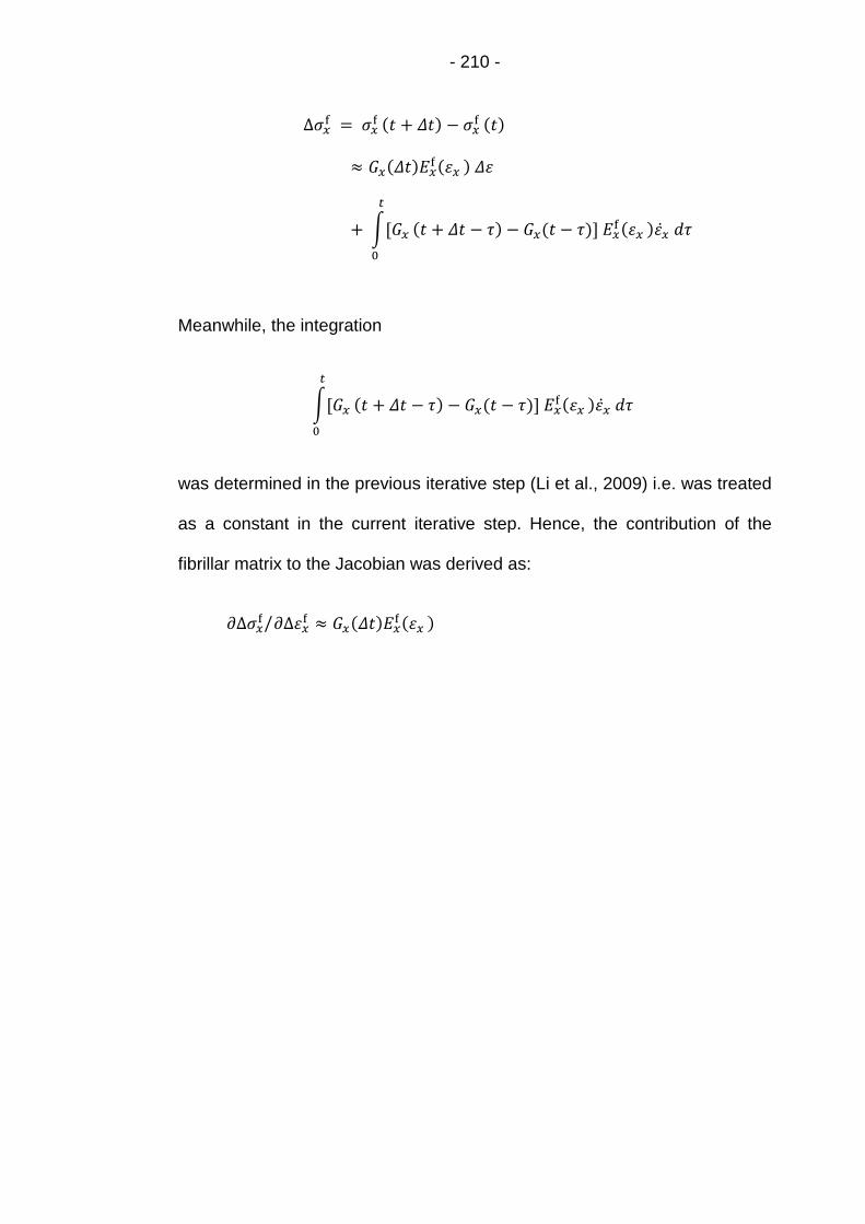
- 210 -
Δߪ௫ = ௫ߪ
(ݐ+ (ݐ߂ − ௫ߪ(ݐ)
≈ ௫ܧ(ݐ߂)௫ܩ(ߝ௫ ) ߝ߂
+ න ௫ܩ]
௧
+ݐ) −ݐ߂ ) − −ݐ)௫ܩ )] ௫ܧ(ߝ௫ ௫ߝ(
Meanwhile, the integration
න ௫ܩ]
௧
+ݐ) −ݐ߂ ) − −ݐ)௫ܩ )] ௫ܧ(ߝ௫ ௫ߝ(
was determined in the previous iterative step (Li et al., 2009) i.e. was treated
as a constant in the current iterative step. Hence, the contribution of the
fibrillar matrix to the Jacobian was derived as:
Δߪ௫ Δߝ௫
/ ≈ ௫ܧ(ݐ߂)௫ܩ(ߝ௫ )