computational logic constraint logic programmingfalaschi/teaching/slidesclp.pdf · constraints born...

Computational Logic

Constraint Logic Programming

1

Constraints

Born within AI: e.g. house design

Constraints used as problem representation:

The man in yellow does not have green eyesThe murderer knows no detective will ever wear dark clothes...

A solution is an assignment which agrees with the initial constraints:

Murderer: Lopez, green eyes, Magnum gun

Or, alternatively, the solution can also be a set of constraints:

The murderer is one of those who had met the cabaret entertainer

(they represent several ground mappings from elements to variables)

There may be no solution:

Natural death

2

A General View

Ancestors:

SKETCHPAD (1963), THINGLAB (1981), Waltz’s algorithm (1965?),MACSYMA (1983), ...

Constraints in logic languages – the origin of “constraint programming”:

General theory developed.

Practical systems, generally based on Prolog + some constraint domain(s).

Constraints in imperative languages:

Equation solving libraries (ILOG)

Timestamping of variables: x := x + 1 ↔ xi+1 := xi + 1

(similar to iterative methods in numerical analysis)

Constraints in functional languages, via extensions:

Evaluation of expressions including free variables.

Absolute Set Abstraction.

3

A comparison with LP (I)

Example (Prolog): q(X, Y, Z) :- Z = f(X, Y).

| ?- q(3, 4, Z).

Z = f(3,4)

| ?- q(X, Y, f(3,4)).

X = 3, Y = 4

| ?- q(X, Y, Z).

Z = f(X,Y)

Example (Prolog): p(X, Y, Z) :- Z is X + Y.

| ?- p(3, 4, Z).

Z = 7

| ?- p(X, 4, 7).

{INSTANTIATION ERROR: in expression}

4

A Comparison with LP (II)

Example (CLP(ℜ)): p(X, Y, Z) :- Z = X + Y.

2 ?- p(3, 4, Z).

Z = 7

*** Yes

3 ?- p(X, 4, 7).

X = 3

*** Yes

4 ?- p(X, Y, 7).

X = 7 - Y

*** Yes

5

A Comparison with LP (III)

Features in CLP:

Domain of computation (reals, integers, booleans, etc).Have to meet some conditions.

Type of constraints allowed for each domain: e.g. arithmetic constraints(+, ∗, =,≤,≥, <, >)

Constraint solving algorithms: simplex, gauss, etc.

LP can be viewed as a constraint logic language over Herbrand terms with asingle constraint predicate symbol: “=”

6

A Comparison with LP (IV)

Advantages:

Helps making programs expressive and flexible.May save much coding.In some cases, more efficient than traditional LP programs due to solverstypically being very efficiently implemented.Also, efficiency due to search space reduction:

LP: generate-and-test.CLP: constrain-and-generate.

Disadvantages:

Complexity of solver algorithms (simplex, gauss, etc) can affect performance.

Solutions:

better algorithmscompile-time optimizations (program transformation, global analysis, etc)parallelism

7

Example of Search Space Reduction

Prolog (generate–and–test):solution(X, Y, Z) :-

p(X), p(Y), p(Z),

test(X, Y, Z).

p(14). p(15). p(16). p(7). p(3). p(11).

test(X, Y, Z) :- Y is X + 1, Z is Y + 1.

Query:

| ?- solution(X, Y, Z).

X = 14

Y = 15

Z = 16 ? ;

no

458 steps (all solutions: 465 steps).

8


CLP(ℜ) (using generate–and–test):solution(X, Y, Z) :-

p(X), p(Y), p(Z),

test(X, Y, Z).

p(14). p(15). p(16). p(7). p(3). p(11).

test(X, Y, Z) :- Y = X + 1, Z = Y + 1.

Query:?- solution(X, Y, Z).

Z = 16

Y = 15

X = 14

*** Retry? y

*** No


9

Generate–and–test Search Tree

A5

Y=14 Y=15

A4 A3 A2 A1

X=15 X=16 X=7 X=3 X=11X=14

Z=14

Z=15

Z=16

Z=7

Z=3

Z=11

g

B5

Y=11Y=3Y=7Y=16

B4 B3 B2 B1

B

A

10


Move test(X, Y, Z) at the beginning (constrain–and–generate):solution(X, Y, Z) :-

test(X, Y, Z),

p(X), p(Y), p(Z).

p(14). p(15). p(16). p(7). p(3). p(11).

Prolog: test(X, Y, Z) :- Y is X + 1, Z is Y + 1.

| ?- solution(X, Y, Z).

{INSTANTIATION ERROR: in expression}

CLP(ℜ): test(X, Y, Z) :- Y = X + 1, Z = Y + 1.

?- solution(X, Y, Z).

Z = 16

Y = 15

X = 14

*** Retry? y

*** No


11

Constrain–and–generate Search Tree

Y=15

X=15 X=16 X=7 X=3 X=11X=14

Z=

16

g

Y=16

12

Constraint Domains

Semantics parameterized by the constraint domain:CLP(X ), where X ≡ (Σ,D,L, T )

Signature Σ: set of predicate and function symbols, together with their arity

L ⊆ Σ–formulae: constraints

D is the set of actual elements in the domain

Σ–structure D: gives the meaning of predicate and function symbols (and hence,constraints).

T a first–order theory (axiomatizes some properties of D)

(D,L) is a constraint domain

Assumptions:

L built upon a first–order language=∈ Σ is identity in D

There are identically false and identically true constraints in L

L is closed w.r.t. renaming, conjunction and existential quantification

13

Domains (I)

Σ = {0, 1, +, ∗, =, <,≤}, D = R, D interprets Σ as usual, ℜ = (D,L)

Arithmetic over the reals

Eg.: x2 + 2xy < yx ∧ x > 0 (≡ xxx + xxy + xxy < y ∧ 0 < x)

Question: is 0 needed? How can it be represented?

Let us assume Σ′ = {0, 1, +, =, <,≤}, ℜLin = (D′,L′)

Linear arithmetic

Eg.: 3x − y < 3 (≡ x + x + x < 1 + 1 + 1 + y)

Let us assume Σ′′ = {0, 1, +, =}, ℜLinEq = (D′′,L′′)

Linear equations

Eg.: 3x + y = 5 ∧ y = 2x

14

Domains (II)

Σ = {<constant and function symbols>, =}

D = { finite trees }

D interprets Σ as tree constructors

Each f ∈ Σ with arity n maps n trees to a tree with root labeled f and whosesubtrees are the arguments of the mapping

Constraints: syntactic tree equality

FT = (D,L)

Constraints over the Herbrand domain

Eg.: g(h(Z), Y ) = g(Y, h(a))

LP ≡ CLP(FT )

15

Domains (III)

Σ = {<constants>, λ, ., ::, =}

D = { finite strings of constants }

D interprets . as string concatenation, :: as string length

Equations over strings of constantsEg.: X.A.X = X.A

Σ = {0, 1,¬,∧, =}

D = {true, false}

D interprets symbols in Σ as boolean functions

BOOL = (D,L)

Boolean constraintsEg.: ¬(x ∧ y) = 1

16

CLP(X ) Programs

Recall that:

Σ is a set of predicate and function symbolsL ⊆ Σ–formulae are the constraints

Π: set of predicate symbols definable by a program

Atom: p(t1, t2, . . . , tn), where t1, t2, . . . , tn are terms and p ∈ Π

Primitive constraint: p(t1, t2, . . . , tn), wheret1, t2, . . . , tn are terms and p ∈ Σ is a predicate symbol

Every constraint is a (first–order) formula built from primitive constraints

The class of constraints will vary (generally only a subset of formulas areconsidered constraints)

A CLP program is a collection of rules of the form a ← b1, . . . , bn where a is anatom and the bi’s are atoms or constraints

A fact is a rule a ← c where c is a constraint

A goal (or query) G is a conjunction of constraints and atoms

17

A case study: CLP(ℜ)

CLP(ℜ) is a language based on Prolog, with the addition of constraint solvingcapabilities over the reals (RLin)

CLP(ℜ) uses the same execution strategy as Prolog (depth–first, left–to–right)

CLP(ℜ) is able to solve directly linear (dis)equations over the reals

Non–linear equations are delayed, waiting for them to eventually become linear

Most relevant feature w.r.t. Prolog (for our purposes): is/2 disappears, and issubsumed by =/2 and (extended) unification

Note: CLP(ℜ) is really CLP((ℜ,FT )) — FT is often omitted

18

Linear Equations (CLP(ℜ))

Vector × vector multiplication (dot product):· : ℜn ×ℜn −→ ℜ

(x1, x2, . . . , xn) · (y1, y2, . . . , yn) = x1 · y1 + · · · + xn · yn

Vectors represented as lists of numbersprod([], [], 0).

prod([X|Xs], [Y|Ys], X * Y + Rest) :-

prod(Xs, Ys, Rest).

Unification becomes constraint solving!?- prod([2, 3], [4, 5], K).

K = 23

?- prod([2, 3], [5, X2], 22).

X2 = 4

?- prod([2, 7, 3], [Vx, Vy, Vz], 0).

Vx = -1.5*Vz - 3.5*Vy

Any computed answer is, in general, an equation over the variables in the query

19

Systems of Linear Equations (CLP(ℜ))

Can we solve systems of equations? E.g.,3x + y = 5

x + 8y = 3

Write them down at the top level prompt:?- prod([3, 1], [X, Y], 5), prod([1, 8], [X, Y], 3).

X = 1.6087, Y = 0.173913

A more general predicate can be built mimicking the mathematical vector notationA · x = b:system(_Vars, [], []).

system(Vars, [Co|Coefs], [Ind|Indeps]) :-

prod(Vars, Co, Ind),

system(Vars, Coefs, Indeps).

We can now express (and solve) equation systems?- system([X, Y], [[3, 1],[1, 8]],[5, 3]).

X = 1.6087, Y = 0.173913

20

Non–linear Equations (CLP(ℜ))

Non–linear equations are delayed

?- sin(X) = cos(X).

sin(X) = cos(X)

This is also the case if there exists some procedure to solve them

?- X*X + 2*X + 1 = 0.

-2*X - 1 = X * X

Reason: no general solving technique is known. CLP(ℜ) solves only linear(dis)equations.

Once equations become linear, they are handled properly:

?- X = cos(sin(Y)), Y = 2+Y*3.

Y = -1, X = 0.666367

Disequations are solved using a modified, incremental Simplex

?- X + Y <= 4, Y >= 4, X >= 0.

Y = 4, X = 0

21

Fibonaci Revisited (Prolog)

Fibonaci numbers:

F0 = 0

F1 = 1

Fn+2 = Fn+1 + Fn

(The good old) Prolog version:fib(0, 0).

fib(1, 1).

fib(N, F) :-

N > 1,

N1 is N - 1,

N2 is N - 2,

fib(N1, F1),

fib(N2, F2),

F is F1 + F2.

Can only be used with the first argument instantiated to a number

22

Fibonaci Revisited (CLP(ℜ))

CLP(ℜ) version: syntactically similar to the previous onefib(0, 0).

fib(1, 1).

fib(N, F1 + F2) :-

N > 1, F1 >= 0, F2 >= 0,

fib(N - 1, F1), fib(N - 2, F2).

Note all constraints included in program (F1 >= 0, F2 >= 0) – good practice!

Only real numbers and equations used (no data structures, no other constraintsystem): “pure CLP(ℜ)”

Semantics greatly enhanced! E.g.?- fib(N, F).

F = 0, N = 0 ;

F = 1, N = 1 ;

F = 1, N = 2 ;

F = 2, N = 3 ;

F = 3, N = 4 ;

23

Analog RLC circuits (CLP(ℜ))

Analysis and synthesis of analog circuits

RLC network in steady state

Each circuit is composed either of:

A simple component, or

A connection of simpler circuits

For simplicity, we will suppose subnetworks connected only in parallel and series−→ Ohm’s laws will suffice (other networks need global, i.e., Kirchoff’s laws)

We want to relate the current (I), voltage (V) and frequency (W) in steady state

Entry point: circuit(C, V, I, W) states that:across the network C, the voltage is V, the current is I and the frequency is W

V and I must be modeled as complex numbers (the imaginary part takes intoaccount the angular frequency)

Note that Herbrand terms are used to provide data structures

24


Complex number X + Y i modeled as c(X, Y)

Basic operations:

c_add(c(Re1,Im1), c(Re2,Im2), c(Re1+Re2,Im1+Im2)).

c_mult(c(Re1, Im1), c(Re2, Im2), c(Re3, Im3)) :-

Re3 = Re1 * Re2 - Im1 * Im2,

Im3 = Re1 * Im2 + Re2 * Im1.

(equality is c equal(c(R, I), c(R, I)), can be left to [extended] unification)

25


Circuits in series:

circuit(series(N1, N2), V, I, W) :-

c_add(V1, V2, V),

circuit(N1, V1, I, W),

circuit(N2, V2, I, W).

Circuits in parallel:

circuit(parallel(N1, N2), V, I, W) :-

c_add(I1, I2, I),

circuit(N1, V, I1, W),

circuit(N2, V, I2, W).

26


Each basic component can be modeled as a separate unit:

Resistor: V = I ∗ (R + 0i)

circuit(resistor(R), V, I, _W) :-

c_mult(I, c(R, 0), V).

Inductor: V = I ∗ (0 + WLi)

circuit(inductor(L), V, I, W) :-

c_mult(I, c(0, W * L), V).

Capacitor: V = I ∗ (0 − 1

WC i)

circuit(capacitor(C), V, I, W) :-

c_mult(I, c(0, -1 / (W * C)), V).

27


Example:

I = 0.65

L = 0.073

C = ?R = ?

V = 4.5

ω = 2400

?- circuit(parallel(inductor(0.073),

series(capacitor(C), resistor(R))),

c(4.5, 0), c(0.65, 0), 2400).

R = 6.91229, C = 0.00152546

?- circuit(C, c(4.5, 0), c(0.65, 0), 2400).

28

The N Queens Problem

Problem:place N chess queens in a N × N board such that they do not attack each other

Data structure: a list holding the column position for each row

The final solution is a permutation of the list [1, 2, ..., N]

E.g.: the solution is represented as [2, 4, 1, 3]

General idea:

Start with partial solution

Nondeterministically select new queen

Check safety of new queen against those already placed

Add new queen to partial solution if compatible; start again with new partialsolution

29

The N Queens Problem (Prolog)

queens(N, Qs) :- queens_list(N, Ns), queens(Ns, [], Qs).

queens([], Qs, Qs).

queens(Unplaced, Placed, Qs) :-

select(Unplaced, Q, NewUnplaced), no_attack(Placed, Q, 1),

queens(NewUnplaced, [Q|Placed], Qs).

no_attack([], _Queen, _Nb).

no_attack([Y|Ys], Queen, Nb) :-

Queen =\= Y + Nb, Queen =\= Y - Nb, Nb1 is Nb + 1,

no_attack(Ys, Queen, Nb1).

select([X|Ys], X, Ys).

select([Y|Ys], X, [Y|Zs]) :- select(Ys, X, Zs).

queens_list(0, []).

queens_list(N, [N|Ns]) :- N > 0, N1 is N - 1, queens_list(N1, Ns).

30

The N Queens Problem (Prolog)

31

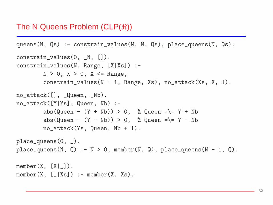
The N Queens Problem (CLP(ℜ))

queens(N, Qs) :- constrain_values(N, N, Qs), place_queens(N, Qs).

constrain_values(0, _N, []).

constrain_values(N, Range, [X|Xs]) :-

N > 0, X > 0, X <= Range,

constrain_values(N - 1, Range, Xs), no_attack(Xs, X, 1).



abs(Queen - (Y + Nb)) > 0, % Queen =\= Y + Nb

abs(Queen - (Y - Nb)) > 0, % Queen =\= Y - Nb

no_attack(Ys, Queen, Nb + 1).

place_queens(0, _).

place_queens(N, Q) :- N > 0, member(N, Q), place_queens(N - 1, Q).

member(X, [X|_]).

member(X, [_|Xs]) :- member(X, Xs).

32


This last program can attack the problem in its most general instance:

?- queens(M,N).

N = [], M = 0 ;

M = [1], M = 1 ;

N = [2, 4, 1, 3], M = 4 ;

N = [3, 1, 4, 2], M = 4 ;

N = [5, 2, 4, 1, 3], M = 5 ;

N = [5, 3, 1, 4, 2], M = 5 ;

N = [3, 5, 2, 4, 1], M = 5 ;

N = [2, 5, 3, 1, 4], M = 5

...

Remark: Herbrand terms used to build the data structures

But also used as constraints (e.g., length of already built list Xs in no attack(Xs,

X, 1))

Note that in fact we are using both ℜ and FT

33


34


CLP(ℜ) generates internally a set of equations for each board size

They are non–linear and are thus delayed until instantiation wakes them up?- constrain_values(4, 4, Q).

Q = [_t3, _t5, _t13, _t21]

_t3 <= 4 0 < abs(-_t13 + _t3 - 2)

_t5 <= 4 0 < abs(-_t13 + _t3 + 2)

_t13 <= 4 0 < abs(-_t21 + _t3 - 3)

_t21 <= 4 0 < abs(-_t21 + _t3 + 3)

0 < _t3 0 < abs(-_t13 + _t5 - 1)

0 < _t5 0 < abs(-_t13 + _t5 + 1)

0 < _t13 0 < abs(-_t21 + _t5 - 2)

0 < _t21 0 < abs(-_t21 + _t5 + 2)

0 < abs(-_t5 + _t3 - 1) 0 < abs(-_t21 + _t13 - 1)

0 < abs(-_t5 + _t3 + 1) 0 < abs(-_t21 + _t13 + 1)

35


Constraints are (incrementally) simplified as new queens are added

?- constrain_values(4, 4, Qs), Qs = [3,1|OQs].

OQs = [_t16, _t24] 0 < abs(-_t24)

Qs = [3, 1, _t16, _t24] 0 < abs(-_t24 + 6)

_t16 <= 4 0 < abs(-_t16)

_t24 <= 4 0 < abs(-_t16 + 2)

0 < _t16 0 < abs(-_t24 - 1)

0 < _t24 0 < abs(-_t24 + 3)

0 < abs(-_t16 + 1) 0 < abs(-_t24 + _t16 - 1)

0 < abs(-_t16 + 5) 0 < abs(-_t24 + _t16 + 1)

Bad choices are rejected using constraint consistency:

?- constrain_values(4, 4, Qs), Qs = [3,2|OQs].

*** No

36

Finite Domains (I)

A finite domain constraint solver associates each variable with a finite subset of Z

I.e., E ∈ {−123,−10..4, 10}

(represented as E :: [-123, -10..4, 10] [Eclipse notation] or as E in {-123}

\/ (-10..4) \/ {10} [SICStus notation])

We can:

Perform arithmetic operations (+, −, ∗, /) on the variables

Establish linear relationships among arithmetic expressions (# =, # <, # =<)

Those operations / relationships are intended to narrow the domains of thevariables

Note: SICStus requires the use of the:- use module(library(clpfd)).

directive in the source code

37

Finite Domains (II)

Example:

?- X #= A + B, A in 1..3, B in 3..7.

X in 4..10, A in 1..3, B in 3..7

The respective minimums and maximums are added

There is no unique solution

?- X #= A - B, A in 1..3, B in 3..7.

X in -6..0, A in 1..3, B in 3..7

The minimum value of X is the minimum value of A minus the maximum value of B

(Similar for the maximum values)

Putting more constraints:

?- X #= A - B, A in 1..3, B in 3..7, X #>= 0.

A = 3, B = 3, X = 0

38

Finite Domains (III)

Some useful primitives in finite domains:

fd min(X, T): the term T is the minimum value in the domain of the variable X

This can be used to minimize (c.f., maximize) a solution?- X #= A - B, A in 1..3, B in 3..7, fd min(X, X).

A = 1, B = 7, X = -6

domain(Variables, Min, Max): A shorthand for several in constraints

labeling(Options, VarList):

instantiates variables in VarList to values in their domains

Options dictates the search order

?- X*X+Y*Y#=Z*Z, X#>=Y, domain([X, Y, Z],1,1000),labeling([],[X,Y,Z]).

X = 4, Y = 3, Z = 5

X = 8, Y = 6, Z = 10

X = 12, Y = 5, Z = 13

...

39

A Project Management Problem (I)

The job whose dependenciesand task lengths are given by:should be finished in 10 timeunits or less

D

E F

0

1 2 3

4

B C

1

0 G

A

Constraints:pn1(A,B,C,D,E,F,G) :-

A #>= 0, G #=< 10,

B #>= A, C #>= A, D #>= A,

E #>= B + 1, E #>= C + 2,

F #>= C + 2, F #>= D + 3,

G #>= E + 4, G #>= F + 1.

40

A Project Management Problem (II)

Query:

?- pn1(A,B,C,D,E,F,G).

A in 0..4, B in 0..5, C in 0..4,

D in 0..6, E in 2..6, F in 3..9, G in 6..10,

Note the slack of the variables

Some additional constraints must be respected as well, but are not shown bydefault

Minimize the total project time:

?- pn1(A,B,C,D,E,F,G), fd min(G, G).

A = 0, B in 0..1, C = 0, D in 0..2,

E = 2, F in 3..5, G = 6

Variables without slack represent critical tasks

41

A Project Management Problem (III)

An alternative setting:

D

E F

0

1 2 3

4

B C

0 G

A

X

We can accelerate task F at some cost

pn2(A, B, C, D, E, F, G, X) :-

A #>= 0, G #=< 10,

B #>= A, C #>= A, D #>= A,

E #>= B + 1, E #>= C + 2,

F #>= C + 2, F #>= D + 3,

G #>= E + 4, G #>= F + X.

We do not want to accelerate it more than needed!

?- pn2(A, B, C, D, E, F, G, X),

fd min(G,G), fd max(X, X).

A = 0, B in 0..1, C = 0, D = 0,

E = 2, F = 3, G = 6, X = 3

42

A Project Management Problem (IV)

We have two independent tasks B and D whose lengths are not fixed:

D

E F

0

2B C

0 G

A

1

Y

4

X

We can finish any of B, D in 2 time units at best

Some shared resource disallows finishing both tasks in 2 time units: they will take6 time units

43

A Project Management Problem (V)

Constraints describing the net:

pn3(A,B,C,D,E,F,G,X,Y) :-

A #>= 0, G #=< 10,

X #>= 2, Y #>= 2, X + Y #= 6,

B #>= A, C #>= A, D #>= A,

E #>= B + X, E #>= C + 2,

F #>= C + 2, F #>= D + Y,

G #>= E + 4, G #>= F + 1.

Query: ?- pn3(A,B,C,D,E,F,G,X,Y), fd min(G,G).

A = 0, B = 0, C = 0, D in 0..1, E = 2, F in 4..5, X = 2, Y = 4, G = 6

I.e., we must devote more resources to task B

All tasks but F and D are critical now

Sometimes, fd min/2 not enough to provide best solution (pending constraints):pn3(A,B,C,D,E,F,G,X,Y),

labeling([ff, minimize(G)], [A,B,C,D,E,F,G,X,Y]).

44

The N-Queens Problem Using Finite Domains (in SICStus Prolog)

By far, the fastest implementationqueens(N, Qs, Type) :-

constrain_values(N, N, Qs),

all_different(Qs), % built-in constraint

labeling(Type,Qs).

constrain_values(0, _N, []).

constrain_values(N, Range, [X|Xs]) :-

N > 0, N1 is N - 1, X in 1 .. Range,

constrain_values(N1, Range, Xs), no_attack(Xs, X, 1).



Queen #\= Y + Nb, Queen #\= Y - Nb, Nb1 is Nb + 1,

no_attack(Ys, Queen, Nb1).

Query. Type is the type of search desired.?- queens(20, Q, [ff]).

Q = [1,3,5,14,17,4,16,7,12,18,15,19,6,10,20,11,8,2,13,9] ?

45

CLP(FT ) (a.k.a. Logic Programming)

Equations over Finite Trees

Check that two trees are isomorphic (same elements in each level)

iso(Tree, Tree).

iso(t(R, I1, D1), t(R, I2, D2)) :-

iso(I1, D2),

iso(D1, I2).

?- iso(t(a, b, t(X, Y, Z)), t(a, t(u, v, W), L)).

L=b, X=u, Y=v, Z=W ? ;

L=b, X=u, Y=W, Z=v ? ;

L=b, W=t(_C,_B,_A), X=u, Y=t(_C,_A,_B), Z=v ? ;

L=b, W=t(_E,t(_D,_C,_B),_A), X=u, Y=t(_E,_A,t(_D,_B,_C)), Z=v ?

46

CLP(WE)

Equations over finite strings

Primitive constraints: concatenation (.), string length (::)

Find strings meeting some property:

?- "123".z = z."231", z::0. ?- "123".z = z."231", z::3.

no no

?- "123".z = z."231", z::1. ?- "123".z = z."231", z::4.

z = "1" z = "1231"

?- "123".z = z."231", z::2.

no

These constraint solvers are very complex

Often incomplete algorithms are used

47

CLP((WE ,Q))

Word equations plus arithmetic over Q (rational numbers)

Prove that the sequence xi+2 = |xi+1| − xi has a period of length 9 (for anystarting x0, x1)

Strategy: describe the sequence, try to find a subsequence such that the periodcondition is violated

Sequence description (syntax is Prolog III slightly modified):seq(<Y, X>). abs(Y, Y) :- Y >= 0.

seq(<Y1 - X, Y, X>.U) :- abs(Y, -Y) :- Y < 0.

seq(<Y, X>.U)

abs(Y, Y1).

Query: Is there any 11–element sequence such that the 2–tuple initial seed isdifferent from the 2–tuple final subsequence (the seed of the rest of thesequence)??- seq(U.V.W), U::2, V::7, W::2, U#W.

fail

48

Summarizing

In general:Data structures (Herbrand terms) for freeEach logical variable may have constraints associated with it (and with othervariables)

Problem modeling :Rules represent the problem at a high level

Program structure, modularityRecursion used to set up constraints

Constraints encode problem conditionsSolutions also expressed as constraints

Combinatorial search problems:CLP languages provide backtracking: enumeration is easyConstraints keep the search space manageable

Tackling a problem:Keep an open mind: often new approaches possible

49

Complex Constraints

Some complex constraints allow expressing simpler constraints

May be operationally treated as passive constraints

E.g.: cardinality operator #(L, [c1, . . . , cn], U) meaning that the number of trueconstraints lies between L and U (which can be variables themselves)

If L = U = n, all constraints must hold

If L = U = 1, one and only one constraint must be true

Constraining U = 0, we force the conjunction of the negations to be true

Constraining L > 0, the disjunction of the constraints is specified

Disjunctive constructive constraint: c1 ∨ c2

If properly handled, avoids search and backtracking

E.g.: nz(X) ← X > 0.

nz(X) ← X < 0.nz(X) ← X < 0 ∨ X > 0.

50

Other Primitives

CLP(X ) systems usually provide additional primitives

E.g.:

enum(X) enumerates X inside its current domain

maximize(X) (c.f. minimize(X)) works out maximum (minimum value) for Xunder the active constraints

delay Goal until Condition specifies when the variables are instantiatedenough so that Goal can be effectively executed

Its use needs deep knowledge of the constraint systemAlso widely available in Prolog systemsNot really a constraint: control primitive

51

Implementation Issues: Satisfiability

Algorithms must be incremental in order to be practical

Incrementality refers to the performance of the algorithm

It is important that algorithms to decide satisfiability have a good average casebehavior

Common technique: use a solved form representation for satisfiable constraints

Not possible in every domain

E.g. in FT constraints are represented in the form x1 = t1(y), . . . , xn = tn(y),where

each ti(y) denotes a term structure containing variables from y

no variable xi appears in y

(i.e., idempotent substitutions, guaranteed by the unification algorithm)

52

Implementation Issues: Backtracking in CLP(X )

Implementation of backtracking more complex than in Prolog

Need to record changes to constraints

Constraints typically stored as an association of variable to expression

Trailing expressions is, in general, costly: cannot be stored at every change

Avoid trailing when there is no choice point between two successive changes

A standard technique: use time stamps to compare the age of the choice pointwith the age of the variable at the time of last trailing

X<Y+Z, Y=Z+W

X<Y+4, Y=4+W, Z=4

X<9, Y=5, Z=4, W=1 trail W, timestamp it

trail X, Y, Z, timestamp them

timestamp X, Y, Z, W

53

Implementation Issues: Extensibility

Constraint domains often implemented now in Prolog-based systems using:

Attributed variables [Neumerkel,Holzbaur]:

Provide a hook into unification.Allow attaching an attribute to a variable.When unification with that variable occurs, user-defined code is called.Used to implement constraint solvers (and other applications, e.g.,distributed execution).

Constraint handling rules (CHRs):

Higher-level abstraction.Allows defining propagation algorithms (e.g., constraint solvers) in ahigh-level way.Often translated to attributed variable-based low-level code.

54

Attributed Variables Example: Freeze

Primitives:attach attribute(X,C)

get attribute(X,C)

detach attribute(X)

update attribute(X,C)

verify attribute(C,T)

combine attributes(C1,C2)

Example: Freezefreeze( X, Goal) :-

attach_attribute( V, frozen(V,Goal)),

X = V.

verify_attribute( frozen(Var,Goal), Value) :-

detach_attribute( Var),

Var = Value,

call(Goal).

combine_attributes( frozen(V1,G1), frozen(V2,G2)) :-

detach_attribute( V1),

detach_attribute( V2),

V1 = V2,

attach_attribute( V1, frozen(V1,(G1,G2))).

55

Programming Tips

Over-constraining:Seems to be against general advice “do not perform extra work”, but canactually cut more space searchSpecially useful if infer is weakOr else, if constraints outside the domain are being used

Use control primitives (e.g., cut) very sparingly and carefully

Determinacy is more subtle, (partially due to constraints in non–solved form)

Choosing a clause does not preclude trying other exclusive clauses(as with Prolog and plain unification)

Compare:max(X,Y,X) :- X > Y. ?- max(X, Y, Z).

max(X,Y,Y) :- X <= Y. Z = X, Y < X ;

withmax(X,Y,X) :- X > Y, !. ?- max(X, Y, Z).

max(X,Y,Y) :- X <= Y. Z = X, Y < X

56

Some Real Systems (I)

CLP defines a class of languages obtained bySpecifying the particular constraint system(s)

Specifying Computation and Selection rules

Most share the Herbrand domain with “=”, but add different domains and/or solveralgorithms

Most use Computation and Selection rules of Prolog

CLP(ℜ):

Linear arithmetic over reals (=,≤, >)

Gauss elimination and an adaptation of Simplex

PrologIII:

Linear arithmetic over rationals (=,≤, >, 6=), Simplex

Boolean (=), 2-valued Boolean Algebra

Infinite (rational) trees (=, 6=)

Equations over finite strings

57

Some Real Systems (II)

CHIP:

Linear arithmetic over rationals (=,≤, >, 6=), Simplex

Boolean (=), larger Boolean algebra (symbolic values)

Finite domains

User–defined constraints and solver algorithms

BNR-Prolog:

Arithmetic over reals (closed intervals) (=,≤, >, 6=), Simplex, propagationtechniques

Boolean (=), 2-valued Boolean algebra

Finite domains, consistency techniques under user–defined strategy

SICStus 3:

Linear arithmetic over reals (=,≤, >, 6=)

Linear arithmetic over rationals (=,≤, >, 6=)

Finite domains (in recent versions)

58

Some Real Systems (III)

ECLiPSe:

Finite domainsLinear arithmetic over reals (=,≤, >, 6=)Linear arithmetic over rationals (=,≤, >, 6=)

clp(FD)/gprolog:

Finite domains

RISC–CLP:

Real arithmetic terms: any arithmetic constraint over realsImproved version of Tarski’s quantifier elimination

Ciao:Linear arithmetic over reals (=,≤, >, 6=)Linear arithmetic over rationals (=,≤, >, 6=)Finite Domains (currently interpreted)

(can be selected on a per-module basis)

59

computational logic constraint logic programmingfalaschi/teaching/slidesclp.pdf · constraints born...

Documents