TitleCOMPUTATIONAL FLUID DYNAMICS WITH MESHADAPTIVITY (Discretization Methods and NumericalAlgorithms for Differential Equations)

Author(s) Tang, Tao; Tang, Huazhong

Citation 数理解析研究所講究録 (2002), 1265: 28-38

Issue Date 2002-05

URL http://hdl.handle.net/2433/42070

Right

Type Departmental Bulletin Paper

Textversion publisher

Kyoto University

COMPUTATIONAL FLUID DYNAMICS WITH MESH ADAPTIVITY *

TAO TANG \dagger AND HUAZHONG TANG \ddagger

Abstract. In this work we demonstrate some recent progress on moving mesh methods with applicationto computational fluid dynamics. The emphasis will be on the application to the gas dynamics governed bythe hyperbolic conservation laws. Several test problems in one- and two dimensions are computed by using themoving mesh methods. The computations demonstrate that the moving mesh methods are efficient for solvingproblems with shock discontinuities, obtaining the same resolution with much less number of grid points thanthe uniform mesh approach.

AMS subject classifications. 65M93,35L64,76Nl0.

Key words. Adaptive mesh method, hyperbolic conservation laws, finite volume method.

1. Introduction. Adaptive mesh methods have important applications for avariety ofphysical and engineering areas such as solid and fluid dynamics, combustion, heat transfer, ma-terial science etc. The physical phenomena in these areas develop dynamicaly singular or nearlysingular solutions in fairly localized regions, such as shock waves, boundary layers, detonationwaves etc. The numerical investigation of these physical problems may require extremely finemeshes over asmall portion of the physical domain to resolve the large solution variations. Inmulti-dimensions, developing effective and robust adaptive grid methods for these problems be-comes necessary. Successful implementation of the adaptive strategy can increase the accuracyof the numerical approximations and also decrease the computational cost. In the past twodecades, there have seen many important progress in moving mesh methods for partial differ-ential equations, including the variational approach of Winslow [22], Brackbill et al. $[2, 3]$ , andRen and Wang [16]; finite element methods of Millers [15]; moving mesh PDEs of Russell et al.$[4, 20]$ , Li and Petzold [11], and Ceniceros and Hou [5]; and moving mesh methods based onharmonic mapping of Dvinsky [8] and Li et al. $[12, 13]$ .

In this work we demonstrate some recent progress on the moving mesh methods with ap-plication to computational fluid dynamics. The emphasis $\mathrm{w}\mathrm{i}\mathbb{I}$ be on the application to the gasdynamics governed by the hyperbolic conservation laws. Harten and Hyman [9] began the earli-est study in this direction, by moving the grid at an adaptive speed in each time step to improvethe resolution of shocks and contact discontinuities. After their work, many other moving meshmethods for hyperbolic problems have been proposed in the literature, including Azarenok andIvanenko [1], Liu et al. [14], Saleri and Steinberg [17], and Stockie et al. [20]. However, it isnoticed that many existing moving mesh methods for hyperbolic problems are designed for onespace dimension. In $\mathrm{I}\mathrm{D}$ , it is generally possible to compute on avery fine grid and so the needfor moving mesh methods may not be clear. Multidimensional moving mesh methods are oftendifficult to use in fluid dynamics problems since the grid will typically suffer large distortions andpossible tangling. It is therefore useful to design asimple and robust moving mesh algorithmfor hyperbolic problems in multi-dimensions.

Following Li et al. [12] we propose amoving mesh method containing two separate parts:PDE time-evolution and mesh-redistribution. The first part can be any suitable high-resolution$\overline{\sim \mathrm{A}}$talk based on this work was presented in RIMS Symposium on Discretization Methods and NumericalAlgorithms for Differential Equations, held from Nov. 14 to 16 at Kyoto University, Japan.

$\uparrow \mathrm{D}\mathrm{e}\mathrm{p}\mathrm{a}\mathrm{r}\mathrm{t}\mathrm{m}\mathrm{e}\mathrm{n}\mathrm{t}$ of Mathematics, The Hong Kong Baptist University, Kowloon Tong, Hong Kong, P. R. China.Em $\mathrm{a}\mathrm{i}\mathrm{l}:\mathrm{t}\mathrm{t}$ algorith $\mathrm{m}$ hkbu. $*\mathrm{d}\mathrm{u}$ .hk

\ddagger The School of Mathematical Sciences, Peking University, Beijing 100871, P. R. China.Em $\mathrm{a}\mathrm{i}\mathrm{l}$ :hztanghath. $\mathrm{p}\mathrm{k}\mathrm{u}.\mathrm{e}\mathrm{d}\mathrm{u}$ .cn

数理解析研究所講究録 1265巻 2002年 28-38

28

T Tang and H-Z Tang

methods such as the wave-propagation algorithm, central schemes, and ENO methods. Oncenumerical solutions are obtained at the given time level, the meshes will be redistributed basedon an iteration procedure. At each iteration, the grids are moved based on avariational prin-ciple and the underlying numerical solutions at the new grids will be updated by using somesimple methods (such as the conventional interpolation). It is noted that the direct use of theconventional interpolation is unsatisfactory for hyperbolic problems, since many physical properties such as mass-conservation and TVD (in $\mathrm{I}\mathrm{D}$ ) may be destroyed. In order to preserve thesephysical properties, we propose to use conservative-interpolation$\mathrm{s}$ in the solution-updating step.This approach also preserves the total mass of the numerical solutions, and by the well-knownLax-Wendroff theory the numerical solutions converge to the weak solution of the underlyinghyperbolic system [21].

2. Mesh generation based on the variational approach. Let $\vec{x}=(x_{1}, x_{2,d}\ldots, x)$ and$\vec{\xi}=$ $(\xi_{1}, \xi_{2}, \cdots, \xi_{d})$ denote the physical and computational coordinates, respectively. Here $d\geq 1$

denotes the number of spatial dimension. A $\mathrm{o}\mathrm{n}\mathrm{e}-\mathrm{t}\mathrm{o}\neg$)ne coordinate transformation from thecomputational (or logical) domain $\Omega_{c}$ to the physical domain $\Omega_{p}$ is denoted by

(2.1) $\vec{x}=\vec{x}(\vec{\xi})$ , $\vec{\xi}\in\Omega_{c}$ .

Its inversion is denoted by

(2.2) $\vec{\xi}=\vec{\xi}(\vec{x})$ , $\vec{x}\in\Omega_{p}$ .

In the variational approach, the mesh map is provided by the minimizer of afunctional of thefollowing form:

(2.3) $E( \vec{\xi})=\frac{1}{2}\sum_{k}\int_{\Omega_{p}}\nabla\xi_{k}^{T}G_{k}^{-1}\nabla\xi_{k}d\vec{x}$ ,

where $\nabla:=$ $(\partial_{x_{1}}, \partial_{x_{2}}, \cdots, \partial_{x_{d}})^{T}$, $G_{k}$ are given symmetric positive definite matrices called moni-tor functions. In general, the monitor functions depend on the underlying solution to be adapted.More terms can be added to the functional (2.3) to control other aspects of the mesh such asorthogonality and mesh alignment with agiven vector field $[2, 3]$ .

The variational mesh is determined by the Euler-Lagrange equation of the above functional:

(2.1) $\nabla\cdot(G_{k}^{-1}\nabla\xi_{k})=0$ , $1\leq k\leq d$.

One of the simplest choices of the monitor functions is $G_{k}=\omega I$ , $1\leq k\leq d$ , where I is theidentity matrix and $\omega$ is apositive weight function, e.g., $\omega$ $=\sqrt{1+|\nabla u|^{2}}$ . Here $u$ is the solutionof the underlying PDE. In this case, we obtain Winslow’s variable diffusion method [22]:

$(2^{J}.5)$ $\nabla\cdot(\frac{1}{\omega}\nabla\xi_{k})=0$, $1\leq k\leq d$ .

By using the above equations, amap between the physical domain $\Omega_{p}$ and the logical domain $\Omega_{c}$

can be computed. Typically, the map transforms auniform mesh in the logical domain to clustergrid points at the regions of the physical domain where the solution has the largest gradients.

Our solution procedure is based on two independent parts: amesh-redistribution algorithmand asolution algorithm. The first part will be based on an iteration procedure to redistributethe mesh points and to interpolate the solution on the underlying new grid points. The secondpart will be independent of the first one, which can be any of the standard codes for solvingthe given PDEs, e.g. finite volume schemes. The solution procedure can be illustrated by thefollowing flowchart:

29

CFD with mesh adaptivity

Algorithm 0.Step 1: Given auniform (fixed) partition of the logical domain Qc, and use Eq. (2.5) to

generate an initial partition $x_{j}^{[0]}:=x_{j}$ of the physical domain $\Omega_{p}$ . Then compute thegrid values $u_{\mathrm{j}+\frac{1}{2}}^{[0]}|$ based on the cell average for the initial data $u(x,0)$ .

11Step 2: Move grid $\{x_{j}^{[\nu]}\}$ to $\{x_{j}^{[\nu+1]}\}$ by solving (2.5) with acouple of Gauss-Seidel iterations.

Then compute $\{u_{j+\frac{1}{2}}^{[\nu+1]}\}$ on the new grid based on aconservative interpolation scheme.Repeat this updating procedure for afixed number of iterations or until $||x^{[\nu+1]}-x^{[\nu]}||$

is sufficiently small.

11Step 3: Evolve the underlying PDEs by using high-resolution finite volume methods on the

mesh $\{x_{j}^{[\nu+1]}\}$ to obtain the numerical approximations $u_{j+\frac{11}{2}}^{n+}$ at the time level $t_{n+1}$ .

Step 4: If $t_{n+1}\leq T$ , then let$u_{j+_{f}^{1}}^{[0]}:=u_{j+_{F}^{1}}^{n+1}\mathrm{n}\mathrm{d}x_{j}^{[0]}11:=x_{j}^{[\nu+1]}$

and go to Step 2.

The detail descriptions on Steps 2and 3, in particular the conservative interpolation formulascan be found in Tang and Tang [21].

3. Numerical experiments. EXAMpLE 3.1. Sod’s problem. In this example, we testour adaptive mesh algorithm to the one–dimensional Euler equations of gas dynamics

(3.1) $\{\begin{array}{l}\rho\rho uE\end{array}\}$

$t+$

$\{\begin{array}{l}\rho u\rho u^{2}+pu(E+p)\end{array}\}$

x

$=0$ ,

where $\rho$ , $u$ , $p$, and $E$ are density, velocity, pressure, and the total energy, respectively. Theabove system is closed by the equation of state, $p=(\gamma-1)(\mathrm{E}-\rho u^{2}/2)$ . The initial data ischosen as

$(\rho, \rho u, E)=\{$(1, 0, 2.5), if $x<0.5$ ,(0.125, 0, 0. 5, if $x>0.5$ .

This is awell-known test problem proposed by Sod [19]. The monitor function in (2.5) used is

(3.2) $\omega=\sqrt{1+\alpha_{1}(\frac{u_{\xi}}{\max_{\xi}|u_{\xi}|})^{2}+\alpha_{2}(\frac{s_{\xi}}{\max_{\xi}|s_{\xi}|})^{2}}$

where $s=p/\rho^{\gamma}$ , and the parameters $\alpha_{i}(i=1,2)$ are some non-negative constants. The abovemonitor function was suggested by Stockie et al. [20] who also discussed several other choicesfor the monitor function. The numerical results are obtained with $J=1\mathrm{O}\mathrm{O}$ , $\alpha_{1}=20,\alpha_{2}=100$

and are presented in Figure 3.1. It is found that the contact and shock discontinuities are wellresolved, although quite anumber of grid points are also moved to the rarefaction wave region.

EXAMpLE 3.2. A $2\mathrm{D}$ Riemann problem. TwO–dimensional Euler equations of gasdynamics can be written as

(3.3) $\{\begin{array}{l}\rho\rho u\rho vE\end{array}\}$ $t+[$

$\rho u$

$\rho u^{2}+p$

$\rho uv$

$u(E+p)$x

$+$ $\{\begin{array}{l}\rho v\rho uv\rho v^{2}+pv(E+p)\end{array}\}$

y

$=0$ ,

30

T. Tang and H -Z. Tang

(a) (b)

(c) (d)

FIG. 3.1. Adaptive mesh solutions at $t=0.2$ for Sod’s shock tube problem, (a): density; (b):velocity; (c): pressure and (d): internal energy, $” 0$”and solid lines denote numerical and exact solutions,respectively.

where $\rho$ , $(u,v)$ , $p$ , and $E$ are density, velocity, pressure, and total energy, respectively. For anideal gas, the equation of state, $p=(\gamma-1)(\mathrm{E}-\rho(u^{2}+v^{2})/2)$ , is provided. The initial data ischosen as

$(\rho, u, v,p)=\{$

(1.1, 0.0, 0.0, 1.1) if $x>0.5$ , $y>0.5$ ,(0.5065, 0.8939, 0.0, 0.35) if $x<0.5$ , $y>0.5$ ,(1.1, 0.8939, 0.8939, 1.1) if $x<0.5$ , $y<0.5$ ,(0.5065, 0.0, 0.8939, 0.35) if $x>0.5$ , $y<0.5$ ,

which corresponds to the case of left forward shock, right backward shock, upper backwardshock, and lower forward shock. We refer the readers to $[10, 18]$ for details.

In [10], Lax and Liu computed $2\mathrm{D}$ Riemann problems with various initial data using thepositive schemes. The problem considered here corresponds to the Configuration 4discusse

31

CFD with mesh adaptivity

1

0.8

o.e

0.4

0.2

$\mathrm{o}$

F1G. 3.2. Example 3.2: The contours of mesh (left) and the density (right). Top: $J_{x}=J_{y}=50$ andbottom: J. $=J_{y}=1\propto$). 30 equally spaced contour lines are used for the density.

in their paper. We use our adaptive mesh algorithm with $(J_{x}, J_{y})=(50,50)$ and $(100, 100)$

to compute this Riemann problem and display the meshes and density at $t=0.25$ in Figure3.2. It is found that our results with $J_{x}=J_{y}=100$ give sharper shock resolution than that ofthe positive schemes with $J_{x}=J_{y}=400$ (see [10], p. 333). The monitor function used in this

computation is $G=\omega I$ with $\omega$ $=\sqrt{1+2(\rho_{\xi}^{2}+\beta_{\eta})}$ .

EXAMpLE 3.3. The double-Mach reflection problem. This problem was studied exten-sively in Woodward and Colella [23] and later by many others. We use exactly the same setup asin [23], i.e. the same initial and boundary conditions and same solution domain $\Omega_{p}=[0,4]\mathrm{x}[0,1]$ .Initially aright-moving Mach 10 shock is positioned at $x= \frac{1}{6}$ , $y=0$ and makes a 60 angl

32

T Tang and H.-Z Tang

F1G 33 $2\mathrm{D}$ double Mach reflection at $t=0.2$:the contours of meshes From top to bottom:$(J_{x}, J_{y})=(80, 20)$ , 160, 40) and 320, 80).

with the $x$-axis. More precisely, the initial data are

$U=\{$$U_{L}$ , for $y\geq h(x, 0)$ ,$U_{R}$ , otherwise,

where the state on the left, the state on the right, and the shock height are

$U_{L}=$ $($ 8, 57.1597, -33.0012, 563.544$)^{T}$ ,$U_{R}=(1.4,0.00.0,2.5)^{T}$ ,$h(x, t)=\sqrt{3}(x-1/6)-20t$ .

33

CFD with mesh adaptivity

$J_{x}=160$ , $J_{y}=40$

$\Leftrightarrow-<$

$\Leftrightarrow-=$

$J_{x}=320$ , $J_{y}=80$

$\mathrm{t}$

$\Leftrightarrow-arrow$

$\Leftrightarrow$

F1G. 3.4. 2D double Mach reflection at t $=0.2$ :the contours of density. From top to bottom:$(J_{x}, J_{y})=(80,$ 20), 160, 40) and 320, 80). 30 equally spaced contour lines are used.

As in [23], only the results in $[0, 3]$ $\mathrm{x}[0,1]$ are displayed. In Figure 3.3, the adaptive mesheswith $(J_{x}, J_{y})=(80,20)$ , 160, 40) and 320, 80) are displayed, while the corresponding contoursof density are displayed in Figure 3.4. By comparing the density plots, it is found the adaptivecomputation results with $(J_{x}, J_{y})=(320,80)$ have similar resolution to the results obtained bythe second-0rder discontinuous Galerkin methods with $(J_{x}, J_{y})=(960,240)$ (p. 214, [7]) and bythe second-0rder central scheme with $(J_{x}, J_{y})=(960,240)$ (p. 67, [7]). Moreover, the adaptiveresults with $(J_{x}, J_{y})=$ 160, 40) have slightly better resolution than the results of fifth orderweighted ENO and the fourth order ENO with $480\cross 119$ grids (p. 406, [7]). Of course, this isnot too surprising since these published results are computed by use of uniform meshes

34

T Tang and H-Z Tang

F1G 35. The adaptive mesh in the whole physical domain for the double Mach reflection problemwith $120\cross 30$ grid points.

Figure 3.5 shows the adaptive mesh in the whole physical domain $[0, 4]\cross[0,1]$ , with $120\cross 30$

grid points. It is observed that less grid points are distributed for $x>3$ , which is adesiredfeature for this test problem. Similar observations are observed for the computations with$80\cross 20,160\cross 40$ and $320\cross 80$ grid points. The monitor function used for this example is takenas $G=\omega I$ with $\omega=\sqrt{1+0.125(\rho_{\xi}^{2}+\rho_{\eta}^{2})}$ .

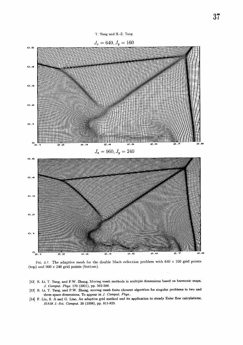
To better appreciate the effectiveness of the adaptive mesh algorithm, we show ablow upportion around the double Mach region in Figure 3.6. The fine details of the complicatedstructure in this region was previously obtained by Cockburn and Shu [6] who used high-0rderdiscontinuous Galerkin methods with $960\cross 240$ and $1920\cross 480$ grid points. In our computations,we used 640 $\cross 160$ and 960 $\cross 240$ grid points. We can see that our result with 960 $\cross 240$

has qualitatively the same resolution as the finer mesh results of the high-0rder discontinuousGalerkin computations. The corresponding mesh contours in the blow up region are shown inFigure 3.7. The smallest $\Delta x$ and $\Delta y$ in these runs are listed in Tables 3.1 and 3.2. It is seen thatratios between the largest and smallest mesh sizes in the adaptive grids are quite large $(\geq 20)$ ,which is adesired feature of the adaptive grid methods.

Acknowledgment. This research was supported by Hong Kong Baptist University andHong Kong Research Grants Council.

REFERENCES

[1] B.N. Azarenok and S. A. Ivanenko, ApPlication of adaPtive grids in numerical analysis of time dePendentProblems in gas dynamics, Comput. Maths. Math. Phys., 40 (2000), PP. 1330149

[2] J.U. Brackbill, An adaptive grid with directional control, J. Comput. Phys. 108 (1993), pp. 38-50.[3] J.U. Brackbill and J.S. Saltzman, Adaptive zoning for singular problems in two dimensions, J. Comput.

Phys. 46 (1982), pp. 342-368.[4] W.M. Cao, W.Z. Huang and R.D. Russell, An $r$-adaptive finite element method based uPon moving mesh

PDEs, J. Comput. Phys. 149 (1999), pp. 221-244.[5] H. D. Ceniceros and T. Y. Hou, An efficient dynamically adaptive mesh for potentially singular solutions.

J. Comput. Phys., 172, 609-639 (2001).[6] B. Cockburn and C.-W. Shu, The Runge Kutta discontinuous Galerkin method for conservation laws V:

multidimensional systems, J. Comput. Phys. 141 (1998), PP. 199-224.[7] B. Cockburn, C. Johnson, C.-W. Shu and E. Tadmor, Advanced Numerical Approximation of Nonlinear

Hyperbolic Equations. Lecture Notes in Math. 1697 (A. Quarteroni ed.). Springer, 1997.[8] A.S. Dvinsky, Adaptive grid generation from harmonic maps on Riemannian manifolds, J. Comput. Phys.

95 (1991), PP. 450-476.

35

CFD with mesh adaptivity

F1G. 3.6. The density contour for the double Mach reflection problem with 640 x160 grid points(top) and $960\cross 240$ grid points (bottom). 45 equally spaced contour lines are used.

[9] A. Harten and J.M. Hyman, Self-adjusting grid methods for one–dimensional hyperbolic conservation laws,J. Comput. Phys. 50(1983), pp. 235-269.

[10] P.D. Lax and X.D. Liu, Solutions of tw0–dimensional Riemann Problems of gas dynamics by positiveschemes, SIAM J. Sci. Comput. 19(1998), pp.319-34O.

[11] S. Li and L. Petzold, Moving mesh methods with uPwinding schemes for time dePendent PDEs, J. Comput.Phys. 131 (1997), pp. 368377.

36

T. Tang and H.-Z. Tang

$\mathcal{J}_{X}=960$ , $J_{y}=240$

FIG. 3.7. The adaptive mesh for the double Mach reflection problem with 640 $\cross 160$ grid points(top) and $960\cross 240$ grid points (bottom).

[12] R. Li, T. Tang, and P.W. Zhang, Moving mesh methods in multiple dimensions based on harmonic maps,J. Comput. Phys. 170 (2001), PP. 562-588.

[13] R. Li, T. Tang, and P.W. Zhang, moving mesh finite element algorithm for singular problems in two and

three space dimensions, To appear in J. Comput Phys..[14] F. Liu, S. Ji and G. Liao, An adaptive grid method and its application to steady Euler flow calculations,

SIAM J. t Sci. Comput 20 (1998), PP. 811-825

37

CFD with mesh adaptivity

TABLE 3. 1The smallest mesh sizes for the double Mach reflection problem with 640 x160 grid points.

T ang 3.2The smallest mesh sizes for the double Mach reflection problem with 960 x240 grid points.

[15] K. Miller and R.N. Miller, Moving finite element. I, SIAM J. Numer Anal. 18(1981), PP. 1019-1032.[16] W.Q. Ren and X.P. Wang, An iterative grid redistribution method for singular problems in multiple di-

mensions, J. Comput. Phys. 159(2000), PP.246-273.[17] K. Saleri and S. Steinberg, Flux-corrected transport in amoving grid. J. Comput. Phys. Ill (1994), pp.

24-32.[18] C.W. Schulz-Rinne, J.P. Collins, and H.M. Glaz, Numerical solution of the Riemann problem for tw0-

dimensional gas dynamics, SIAM J. Sci. Comput. 14(1993), pp.1394-1414.[19] G. A. Sod, Asurvey of finite difference methods for systems of nonlinear hyPerbolic conservation laws. J.

Comput. Phys. 27 (1978), 1-31.[20] J.M. Stockie, J.A. Mackenzie, and $\dot{\mathrm{R}}.\mathrm{D}$ . Russell, Amoving mesh method for one–dimensional hyPerbolic

conservation laws, SIAM J. Sci. Comput, 22 (2001), PP. 1791-1813.[21] H.-Z. Tang and T. Tang, Adaptive Mesh Methods for One- and TwO-Dimensional HyPerbolic Conservation

Laws, PrePrint, 2001. Available in http: $//\mathrm{w}\mathrm{w}\mathrm{w}$ .math.ntnu. $\mathrm{n}\mathrm{o}/\mathrm{c}\mathrm{o}\mathrm{n}\mathrm{s}\mathrm{e}\mathrm{r}\mathrm{v}\mathrm{a}\mathrm{t}\mathrm{i}\mathrm{o}\mathrm{n}/2001/014$ .html.[22] A. Winslow, Numerical solution of the quasi-linear Poisson equation, J. ComPut. Phys. 1(1967), pp.149-

172.[23] P. Woodward and P. Colella, The numerical simulation of two dimensional fluid flow with strong shocks,

J. Comput. Phys. 54 (1984), PP. 115-173

38