COMPUTATIONAL FLUID DYNAMICS ANALYSIS OF STORE SEPARATION

A THESIS SUBMITTED TOTHE GRADUATE SCHOOL OF NATURAL AND APPLIED SCIENCES

OFTHE MIDDLE EAST TECHNICAL UNIVERSITY

BY

H. OZGUR DEMIR

IN PARTIAL FULFILLMENT OF THE REQUIREMENTSFOR

THE DEGREE OF MASTER OF SCIENCEIN

AEROSPACE ENGINEERING

AUGUST 2004

Approval of the Graduate School of Natural and Applied Sciences.

Prof. Dr. Canan OzgenDirector

I certify that this thesis satisfies all the requirements as a thesis for the degree ofMaster of Science.

Prof. Dr. Nafız AlemdarogluHead of Department

This is to certify that we have read this thesis and that in our opinion it is fullyadequate, in scope and quality, as a thesis for the degree of Master of Science.

Prof. Dr. Nafız AlemdarogluSupervisor

Examining Committee Members

Prof. Dr. Kahraman Albayrak

Prof. Dr. Nafız Alemdaroglu

Assoc. Prof. Dr. Sinan Eyi

Assoc. Prof. Dr. Serkan Ozgen

Assoc. Prof. Dr. Yusuf Ozyoruk

I hereby declare that all information in this document has been ob-

tained and presented in accordance with academic rules and ethical

conduct. I also declare that, as required by these rules and conduct,

I have fully cited and referenced all material and results that are not

original to this work.

Name, Last name : H. Ozgur Demir

Signature :

iii

ABSTRACT

COMPUTATIONAL FLUID DYNAMICS ANALYSIS OF STORE

SEPARATION

Demır, H. Ozgur

M.S., Department of Aerospace Engineering

Supervisor: Prof. Dr. Nafız Alemdaroglu

August 2004, 83 pages

In this thesis, store separation from two different configurations are solved us-

ing computational methods. Two different commercially available CFD codes;

CFD-FASTRAN, an implicit Euler solver, and an unsteady panel method solver

USAERO, coupled with integral boundary layer solution procedure are used for

the present computations. The computational trajectory results are validated

against the available experimental data of a generic wing-pylon-store configura-

tion at Mach 0.95. Major trends of the separation are captured. Same configura-

tion is used for the comparison of unsteady panel method with Euler solution at

Mach 0.3 and 0.6. Major trends are similar to each other while some differences

iv

in lateral and longitudinal displacements are observed. Trajectories of a fueltank

separated from an F-16 fighter aircraft wing and full aircraft configurations are

found at Mach 0.3 using only the unsteady panel code. The results indicate that

the effect of fuselage is to decrease the drag and to increase the side forces acting

on the separating fuel tank from the aircraft. It is also observed that the yawing

and rolling directions of the separating fueltank are reversed when it is separated

from the full aircraft configuration when compared to the separation from the

wing alone configuration.

Keywords: CFD, Store Separation, Chimera, Overset Grids, CFD-FASTRAN,

USAERO, Euler, Panel method

v

OZ

HARICI YUK AYRILMASININ HESAPLAMALI AKISKANLAR DINAMIGI

ILE ANALIZI

Demır, H. Ozgur

Yuksek Lisans, Havacılık ve Uzay Muhendisligi Bolumu

Tez Yoneticisi: Prof. Dr. Nafız Alemdaroglu

Agustos 2004, 83 sayfa

Bu calısmada, iki farklı konfigurasyondan harici yuk ayrılması problemi hesapla-

malı akıskanlar yontemleri kullanılarak cozulmustur. Sonucların elde edilmesinde

iki farklı hesaplamalı akıskanlar dinamigi ticari yazılım paketi kullanılmıstır.

Bunlar, CFD-FASTRAN Euler cozucusu, ve zamana baglı panel metodu ile bir-

likte entegral sınır tabaka yontemini kullanan USAERO’dur. Jenerik kanat-pilon-

harici yuk konfigurasyonunun Mach 0.95 akıs sartlarında hesaplanan yorunge

sonucları, ruzgar tuneli test sonucları ile karsılastırılmıstır. Ayrılma esnasındaki

onemli degisimler, hesaplamalı akıskanlar dinamigi yontemleri ile gozlenmistir.

Aynı konfigurasyon, Mach 0.3 ve 0.6 akıs sartlarında zamana baglı panel metodu

vi

ve Euler cozumlerinin karsılastırılmasında da kullanılmıstır. Yorunge uzerindeki

temel degisimler birbirine benzer olup yanal ve boylamsal yondeki yerdegistirme-

lerde farklılıklar gorulmustur. F-16 savas ucagının kanadına ve tum ucaga ait

konfigurasyonlardan Mach 0.3 akıs sartlarında ayrılan bir yakıt tankının izledigi

yorunge, zamana baglı panel metodu ile bulunmustur. Ucak govdesinin yakıt

tankının ayrılmasına olan etkisi, yakıt tankı uzerine etkiyen surukleme kuvve-

tinin azalması ve yanal kuvvetin artması yonundedir. Aynı ayrılma durumunda,

yakıt tankının ayrılma sonrasındaki sapma ve yalpalama hareketlerinin yonlerinin

de degistigi gozlenmistir.

Anahtar Kelimeler: HAD, Harici Yuk Ayrılması, Chimera, Ust Uste Binen Ag

Sistemi, CFD-FASTRAN, USAERO, Euler, Panel metodu

vii

to my family, for their endless support...

viii

ACKNOWLEDGMENTS

I want to state my thanks to

Prof. Dr. Nafiz Alemdaroglu for his supervision, encouragement and patience

during all stages of this thesis. His great ability to foresee the future needs of our

country makes this thesis valuable for all whom interested in this subject.

Assoc. Prof. Dr. Yusuf Ozyoruk for his support, comments and suggestions,

and Prof. Dr. Ismail Hakkı Tuncer for his technical support about the hardware

and software needs during this thesis.

My friends from Aerospace Engineering Department, especially to Mustafa

Kaya for his endless technical assistance and moral support in all of the stages

of this thesis. His endless effort is highly appreciated. I would like to extend my

thanks to D. Funda Kurtulus for her support and help in the learning stages of

the software, to Y. Barbaros Ulusoy for being a right hand for me when I needed

help, to Omer Onur and Ozhan Oksuz for their useful suggestions and friendship.

Erhan Tarhan for his suggestions and precious contribution to this thesis. I

would like to thank to Keith Jordan from CFDRC for his invaluable suggestions

and comments.

ASELSAN A.S. for providing the necessary software and hardware. I extend

my special thanks to Mr. Vahit Ozveren for his support.

My friends Haluk Erhan from TUAF and Bulent Sumer from Tubitak-SAGE

for their suggestions, and their precious brotherhood for all the time.

My dear family, my grandmother and my cousin Evrim for their smiling faces

all the time with their endless support, patience and help during this thesis.

My precious Mine Dogan, for being a shining light with her worthy knowledge

and intelligence, and for being a little child to remind me the beauty of life.

ix

TABLE OF CONTENTS

PLAGIARISM . . . . . . . . . . . . . . . . . . . . . . . . . . . . . . . . . iii

ABSTRACT . . . . . . . . . . . . . . . . . . . . . . . . . . . . . . . . . . iv

OZ . . . . . . . . . . . . . . . . . . . . . . . . . . . . . . . . . . . . . . . . vi

DEDICATON . . . . . . . . . . . . . . . . . . . . . . . . . . . . . . . . . . viii

ACKNOWLEDGMENTS . . . . . . . . . . . . . . . . . . . . . . . . . . . ix

TABLE OF CONTENTS . . . . . . . . . . . . . . . . . . . . . . . . . . . x

LIST OF TABLES . . . . . . . . . . . . . . . . . . . . . . . . . . . . . . . xiii

LIST OF FIGURES . . . . . . . . . . . . . . . . . . . . . . . . . . . . . . xiv

LIST OF SYMBOLS . . . . . . . . . . . . . . . . . . . . . . . . . . . . . . xvii

CHAPTER

1 INTRODUCTION . . . . . . . . . . . . . . . . . . . . . . . . . . 1

1.1 Overview . . . . . . . . . . . . . . . . . . . . . . . . . . . 1

1.2 Historical Background of Store Separation Testing . . . . 3

1.3 Literature Survey . . . . . . . . . . . . . . . . . . . . . . 5

1.4 Thesis Scope and Outline . . . . . . . . . . . . . . . . . . 7

2 THEORETICAL BACKGROUND . . . . . . . . . . . . . . . . . 10

2.1 Overview . . . . . . . . . . . . . . . . . . . . . . . . . . . 10

2.2 CFD-FASTRAN Flow Solver . . . . . . . . . . . . . . . . 12

2.2.1 Governing Equations . . . . . . . . . . . . . . . 12

2.2.2 Space and Time Discretization . . . . . . . . . . 13

2.2.3 Initial and Boundary Conditions . . . . . . . . . 14

2.3 USAERO Panel Code . . . . . . . . . . . . . . . . . . . . 16

2.3.1 Governing Equations . . . . . . . . . . . . . . . 16

x

2.3.2 Wall Boundry Conditions . . . . . . . . . . . . . 17

2.3.3 Surface Pressure Calculation . . . . . . . . . . . 17

2.3.4 Wake Treatment . . . . . . . . . . . . . . . . . . 18

3 FLOW SOLVER . . . . . . . . . . . . . . . . . . . . . . . . . . . 19

3.1 Overview . . . . . . . . . . . . . . . . . . . . . . . . . . . 19

3.2 Geometry Creation . . . . . . . . . . . . . . . . . . . . . . 20

3.3 Structured Grid Generation . . . . . . . . . . . . . . . . . 20

3.4 CHIMERA Methodology . . . . . . . . . . . . . . . . . . 21

3.4.1 Searching Process . . . . . . . . . . . . . . . . . 23

3.4.2 Hole-Cutting Process . . . . . . . . . . . . . . . 23

3.4.3 Interpolation Algorithm . . . . . . . . . . . . . . 25

3.4.4 Setup and Application . . . . . . . . . . . . . . . 25

3.5 Parallel Execution . . . . . . . . . . . . . . . . . . . . . . 26

3.5.1 Setup and Application Process . . . . . . . . . . 27

3.6 Moving Body Module and 6DOF Equations . . . . . . . . 28

3.7 Output Data . . . . . . . . . . . . . . . . . . . . . . . . . 29

4 FLOW SOLVER VALIDATION TEST CASES . . . . . . . . . . 31

4.1 Overview . . . . . . . . . . . . . . . . . . . . . . . . . . . 31

4.2 Chimera Validation Test Cases . . . . . . . . . . . . . . . 32

4.2.1 Store Alone Case . . . . . . . . . . . . . . . . . 33

4.2.2 Two Stores Side-by-Side Case . . . . . . . . . . . 33

4.3 Wing-Store Test Case . . . . . . . . . . . . . . . . . . . . 35

4.4 Store Separation Test Case . . . . . . . . . . . . . . . . . 39

4.4.1 Configuration Geometry . . . . . . . . . . . . . . 39

4.4.1.1 Wing Geometry . . . . . . . . . . . . 39

4.4.1.2 Pylon Geometry . . . . . . . . . . . . 39

4.4.1.3 Store Geometry . . . . . . . . . . . . 41

4.4.2 Grids of the Configuration Geometry . . . . . . 42

4.4.2.1 Wing-Pylon Domain . . . . . . . . . 42

4.4.2.2 Store Domain . . . . . . . . . . . . . 43

4.4.2.3 Overlapping Wing-Pylon and Store Grids 43

4.4.3 Solution Parameters . . . . . . . . . . . . . . . . 45

4.4.3.1 Initial and Boundary Conditions . . . 45

xi

4.4.3.2 Solver Settings . . . . . . . . . . . . 46

4.4.3.3 Convergence Criterion . . . . . . . . 47

4.4.3.4 Chimera Parameters . . . . . . . . . 48

4.4.3.5 Transient Solution and Moving BodyParameters . . . . . . . . . . . . . . 49

4.4.4 Separation Results of the Wing-Pylon-Store TestCase . . . . . . . . . . . . . . . . . . . . . . . . 51

4.4.4.1 Linear and Angular Displacements ofthe Store . . . . . . . . . . . . . . . . 51

4.4.4.2 Linear and Angular Velocities of theStore . . . . . . . . . . . . . . . . . . 53

4.4.4.3 Forces Acting on the Store . . . . . . 54

4.4.4.4 Separation Results Without Sting . . 56

5 RESULTS AND DISCUSSION . . . . . . . . . . . . . . . . . . . 60

5.1 Overview . . . . . . . . . . . . . . . . . . . . . . . . . . . 60

5.2 Configurations . . . . . . . . . . . . . . . . . . . . . . . . 60

5.2.1 Wing-Pylon-Store Configuration . . . . . . . . . 61

5.2.1.1 Grids and Paneling . . . . . . . . . . 62

5.2.1.2 Computations . . . . . . . . . . . . . 62

5.2.1.3 Smooth base-Sharp Cut base ForceComparisons . . . . . . . . . . . . . . 63

5.2.2 F-16 Aircraft Configurations . . . . . . . . . . . 64

5.3 Results . . . . . . . . . . . . . . . . . . . . . . . . . . . . 66

5.3.1 Wing-Pylon-Store Separation Results . . . . . . 66

5.3.2 Fueltank Separation Results from F-16 Aircraft 72

6 CONCLUDING REMARKS . . . . . . . . . . . . . . . . . . . . . 76

REFERENCES . . . . . . . . . . . . . . . . . . . . . . . . . . . . . . . . . 81

xii

LIST OF TABLES

TABLE

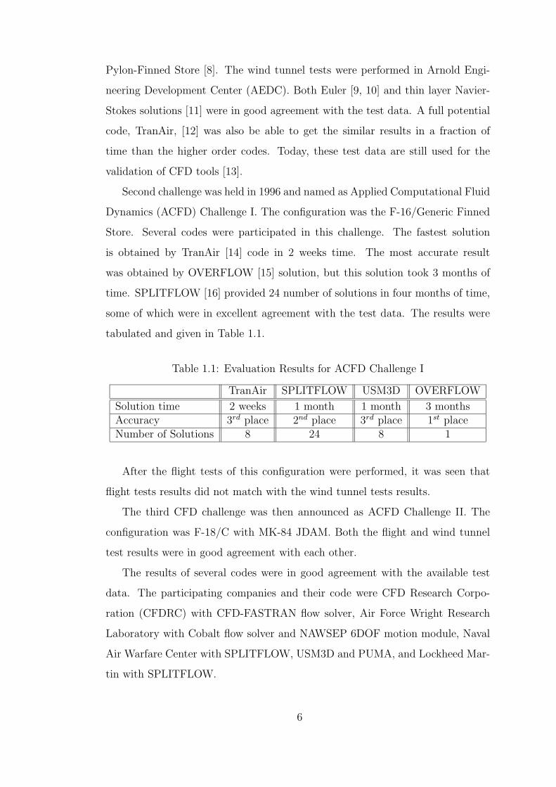
1.1 Evaluation Results for ACFD Challenge I . . . . . . . . . . . . . . 6

4.1 Memory need and CPU time comparisons of CFD-FASTRAN andEuler Solver[33] . . . . . . . . . . . . . . . . . . . . . . . . . . . . 36

4.2 Freestream Flow values for the validation test case . . . . . . . . 464.3 Solution parameters used in the Wing-Pylon-Store validation case[21] 50

5.1 Force coefficients on the store in its captive position, smooth andsharp-cut base comparisons, M=0.3 . . . . . . . . . . . . . . . . . 64

5.2 Moment coefficients on the store wrt. c.g. location in its captiveposition, smooth and sharp-cut base comparisons, M=0.3 . . . . . 64

5.3 Summary of the force and moment coefficients acting on the storein its captive carriage position, comparison of USAERO and CFD-FASTRAN solutions at M=0.3 . . . . . . . . . . . . . . . . . . . . 72

5.4 Summary of the force and moment coefficients acting on the storein its captive carriage position, comparison of USAERO and CFD-FASTRAN solutions at M=0.6 . . . . . . . . . . . . . . . . . . . . 72

5.5 Summary of the force and moment coefficients acting on the fu-eltank in its captive carriage position right before separation, M=0.3 75

xiii

LIST OF FIGURES

FIGURES

1.1 Collision of a fueltank with the aircraft after its separation, picturesare taken from the movie of the flight test (ordered from left to right) 2

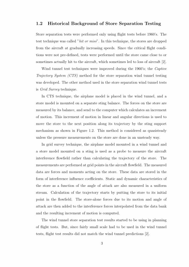
1.2 Picture from a store separation testing using Captive TrajectorySystem in Arnold Engineering Development Center, showing theinstant positions of the store during separation . . . . . . . . . . . 4

1.3 Relation between CFD, wind tunnel and flight tests . . . . . . . . 5

3.1 Steps of hole-cutting process for wall boundaries of wing in thestore domain, sectional cut through store center in 3D . . . . . . . 24

3.2 Selection of overlapping zones for the major zone using GUI . . . 263.3 Coupling 6DOF calculations with the flow solver using Moving

Body Module . . . . . . . . . . . . . . . . . . . . . . . . . . . . . 29

4.1 Overlapping grids of store with the background grid . . . . . . . 324.2 Hole-cut in the background domain for the store . . . . . . . . . . 334.3 Comparison of pressure coefficient distribution on the store with

experimental data [32], one store configuration, M=0.95 . . . . . . 344.4 Overlapping grids and hole-cutting through a section . . . . . . . 344.5 Comparison of pressure coefficient distribution on the store with

experimental data[32], two stores side-by-side configuration, M=0.95 354.6 Mesh view for the wing-store configuration [33] . . . . . . . . . . 364.7 Pressure distributions on the store and comparison to [33] . . . . 374.8 Lower and upper surface pressures of the wing, comparison of re-

sults with [33] . . . . . . . . . . . . . . . . . . . . . . . . . . . . . 384.9 General Views of the Wing-Pylon-Store Configuration . . . . . . . 404.10 Detailed Drawing of the Pylon . . . . . . . . . . . . . . . . . . . . 404.11 Detailed Drawing of the Store . . . . . . . . . . . . . . . . . . . . 414.12 Sectional cut at the root of the wing-pylon domain . . . . . . . . 424.13 Store grid topology through sectional cuts . . . . . . . . . . . . . 434.14 Store domain, grids showing the outer chimera boundary . . . . . 434.15 Overlapping store and wing-pylon domains . . . . . . . . . . . . . 444.16 Grid around the store, between the store and the pylon . . . . . . 454.17 Comparison of the solutions with different grid resolutions to each

other and to experimental data [8] using the pressure coefficientdistribution on the store, wing-pylon-store case, M=0.95 . . . . . 46

4.18 Hole-cut in the store domain for the wing . . . . . . . . . . . . . . 47

xiv

4.19 First and second order spatial accuracy effect on the pressure dis-tribution . . . . . . . . . . . . . . . . . . . . . . . . . . . . . . . . 48

4.20 Steady state solution residual graphs, wing-pylon-store test case . 484.21 Main steps taken in the solution of the store separation problem 494.22 Comparison of linear displacements of the store with the experi-

mental data[8], wing-pylon-store validation case, M=0.95 . . . . . 514.23 Comparison of angular displacements of the store with the exper-

imental data[8], wing-pylon-store validation case, M=0.95 . . . . . 524.24 Comparison of linear velocities of the store with the experimental

data[21], wing-pylon-store validation case, M=0.95 . . . . . . . . . 534.25 Comparison of angular velocities of the store with the experimental

data[8], wing-pylon-store validation case, M=0.95 . . . . . . . . . 544.26 Comparison of force coefficients of the store with the experimental

data[8], wing-pylon-store validation case, M=0.95 . . . . . . . . . 554.27 Sting effect on the linear displacements of the store, wing-pylon-

store validation case, M=0.95 . . . . . . . . . . . . . . . . . . . . 564.28 Sting effect on the angular displacements of the store, wing-pylon-

store validation case, M=0.95 . . . . . . . . . . . . . . . . . . . . 574.29 Sting effect on angular velocities of the store, wing-pylon-store val-

idation case, M=0.95 . . . . . . . . . . . . . . . . . . . . . . . . . 584.30 Sting effect on force coefficients acting on the store, wing-pylon-

store validation case, M=0.95 . . . . . . . . . . . . . . . . . . . . 58

5.1 Side view of wing-pylon-store configuration, sharp cut-base (left)and smooth-base (right) . . . . . . . . . . . . . . . . . . . . . . . 61

5.2 Paneling and wake modeling of wing-pylon-store configuration forUSAERO . . . . . . . . . . . . . . . . . . . . . . . . . . . . . . . 63

5.3 F-16 Wing-Pylon-Store configuration . . . . . . . . . . . . . . . . 655.4 F-16 aircraft full configuration paneling and wake modeling . . . . 665.5 Linear displacements of the store after separation, comparison of

CFD-FASTRAN and USAERO solutions at M=0.3 . . . . . . . . 675.6 Linear displacements of the store after separation,comparison of

CFD-FASTRAN and USAERO solutions at M=0.6 . . . . . . . . 685.7 Angular displacements of the store with respect to its body axis

after separation, comparison of CFD-FASTRAN and USAERO so-lutions at Mach 0.3 . . . . . . . . . . . . . . . . . . . . . . . . . . 69

5.8 Angular displacements of the store with respect to its body axisafter separation, comparison of CFD-FASTRAN and USAERO so-lutions at Mach 0.6 . . . . . . . . . . . . . . . . . . . . . . . . . . 69

5.9 Pressure distribution on the store in its captive position, compar-ison of USAERO and CFD-FASTRAN solutions at M=0.3 . . . . 70

5.10 Pressure distribution on the store in its captive position, compar-ison of USAERO and CFD-FASTRAN solutions at M=0.6 . . . . 70

5.11 Time Histories of force coefficients acting on the store along itstrajectory, comparison of USAERO and CFD-FASTRAN solutionsat M=0.3, M=0.6 . . . . . . . . . . . . . . . . . . . . . . . . . . . 71

5.12 Linear displacements of the fueltank after separation, M=0.3 . . . 73

xv

5.13 Angular displacements of the fueltank after separation with respectto its body axis, M=0.3 . . . . . . . . . . . . . . . . . . . . . . . 74

5.14 Pressure distributions on the fueltank in captive position, M=0.3 745.15 Time histories of force coefficients acting on the fueltank along its

trajectory, M=0.3 . . . . . . . . . . . . . . . . . . . . . . . . . . . 75

xvi

LIST OF SYMBOLS

ROMAN SYMBOLS

b Wing span

c Chord length

Cp Pressure coefficient

CFx, Force coefficient in x,

CFy, in y,

CFz in z direction

CMx, Moment coefficient in x,

CMy, in y,

CMz in z direction

e0 Total energy per unit vol-ume

~F Resultant force vector

~Fc Convective flux vector

~h Angular momentum vector

Ixx Roll moment of inertia

Iyy Pitch moment of inertia

Izz Yaw moment of inertia

L2 Least-squares error norm

m mass

M Mach Number

~M Resultant moment vector

~n Unit normal vector to sur-face

nx, ny, Cartesian components

nz of the surface unit normal

P,Q,R Roll, yaw, pitch angular rates

p Pressure

Q Conserved state vector

S Surface

t Time

u, v, w Cartesian velocity compo-nents

~v Perturbation velocity

~vg Volume surface velocity

V Volume

~V Velocity vector

Vb Translational velocity of thebody

Vs Surface point velocity

V∞ Free stream velocity

x, y, z Cartesian coordinates

X/L Body axial location/bodylength

GREEK SYMBOLS

γ Specific heat ratio

ρ Density

τ Non-dimensional time

φ Velocity potential

φ, Roll,

θ, Yaw,

ψ Pitch angular position ofthe store

~ω Rotational velocity vector

~Ω Rotational velocity vector

xvii

~∇ Gradient operator

∇2 Laplacian operator

SUBSCRIPTS

b Body

c Cell adjacent to wall

n Time step

s Surface

w Wall

∞ Freestream value

ACRONYMS

ACFD Applied Computational FluidDynamics

ADT Alternating Digital Tree

AEDC Arnold Engineering Devel-opment Center

BC Boundary Condition

CAD Computer Aided Design

CFD Computational Fluid Dy-namics

CFDRC Computational Fluid Dy-namics Research Cooper-ation

CFL Courant-Friedrichs-Lewy Num-ber

CPU Central Processing Unit

CTS Captive Trajectory System

DOF Degree of Freedom

FDS Flux Difference Splitting

FV S Flux Vector Splitting

GUI Graphical User Interface

IGES Initial Graphics ExchangeSpecifications

IFM Influence Function Method

JDAM Joint Direct Attack Muni-tion

MDICE Multi-Disciplinary Comput-ing Environment

NURBS Non-Uniform Rational B-Splines

xviii

CHAPTER 1

INTRODUCTION

1.1 Overview

During World War I, a pilot or a bombardier could simply toss a bomb safely clear

of his aircraft since the cockpit is open to air and no other mechanism rather than

the pilot’s hand was used for the ejection of the bomb. Safe Separation problem

has been raised whenever the cockpit was enclosed and wide variety of bombs

and stores with different kinds of ejection methods were started to be used in the

aircraft industry [1].

Whenever a store is released in flight, it is supposed to clear the carrying

aircraft without hitting or damaging it. In many situations, the precise point at

which the store impacts on the ground is not of interest; the only requirement

of the safe separation process is that the store does not collide with the aircraft.

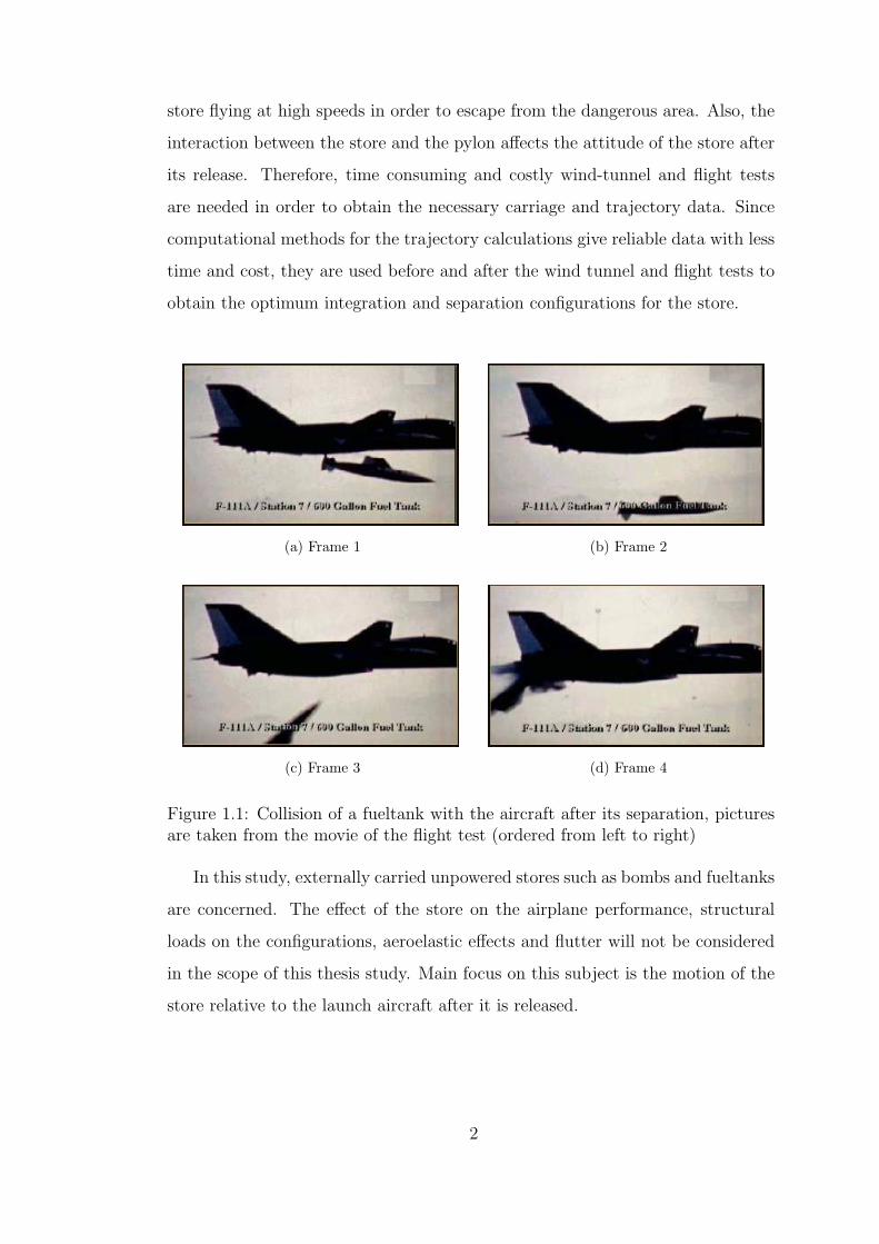
Pictures showing the collision of a 600 gallon fueltank with an F-111/A aircraft

after its separation are given in Figure 1.1.

Safe separation of a store from an aircraft is one of the major aerodynamic

problems in the design and in the integration of a new store to an aircraft. Car-

riage loads and moments acting on the store should be correctly predicted in order

to have an idea about its behavior after separation. It is difficult to predict the

aircraft flowfield correctly, especially in the transonic regimes since the flowfield

is highly dominated by shocks [2]. However, fighter aircrafts prefer to eject the

1

store flying at high speeds in order to escape from the dangerous area. Also, the

interaction between the store and the pylon affects the attitude of the store after

its release. Therefore, time consuming and costly wind-tunnel and flight tests

are needed in order to obtain the necessary carriage and trajectory data. Since

computational methods for the trajectory calculations give reliable data with less

time and cost, they are used before and after the wind tunnel and flight tests to

obtain the optimum integration and separation configurations for the store.

(a) Frame 1 (b) Frame 2

(c) Frame 3 (d) Frame 4

Figure 1.1: Collision of a fueltank with the aircraft after its separation, picturesare taken from the movie of the flight test (ordered from left to right)

In this study, externally carried unpowered stores such as bombs and fueltanks

are concerned. The effect of the store on the airplane performance, structural

loads on the configurations, aeroelastic effects and flutter will not be considered

in the scope of this thesis study. Main focus on this subject is the motion of the

store relative to the launch aircraft after it is released.

2

1.2 Historical Background of Store Separation Testing

Store separation tests were performed only using flight tests before 1960’s. The

test technique was called ”hit or miss”. In this technique, the stores are dropped

from the aircraft at gradually increasing speeds. Since the critical flight condi-

tions were not pre-defined, tests were performed until the store came close to or

sometimes actually hit to the aircraft, which sometimes led to loss of aircraft [2].

Wind tunnel test techniques were improved during the 1960’s; the Captive

Trajectory System (CTS) method for the store separation wind tunnel testing

was developed. The other method used in the store separation wind tunnel tests

is Grid Survey technique.

In CTS technique, the airplane model is placed in the wind tunnel, and a

store model is mounted on a separate sting balance. The forces on the store are

measured by its balance, and send to the computer which calculates an increment

of motion. This increment of motion in linear and angular directions is used to

move the store to the next position along its trajectory by the sting support

mechanism as shown in Figure 1.2. This method is considered as quasisteady

unless the pressure measurements on the store are done in an unsteady way.

In grid survey technique, the airplane model mounted in a wind tunnel and

a store model mounted on a sting is used as a probe to measure the aircraft

interference flowfield rather than calculating the trajectory of the store. The

measurements are performed at grid points in the aircraft flowfield. The measured

data are forces and moments acting on the store. These data are stored in the

form of interference influence coefficients. Static and dynamic characteristics of

the store as a function of the angle of attack are also measured in a uniform

stream. Calculation of the trajectory starts by putting the store to its initial

point in the flowfield. The store-alone forces due to its motion and angle of

attack are then added to the interference forces interpolated from the data bank

and the resulting increment of motion is computed.

The wind tunnel store separation test results started to be using in planning

of flight tests. But, since fairly small scale had to be used in the wind tunnel

tests, flight test results did not match the wind tunnel predictions [2].

3

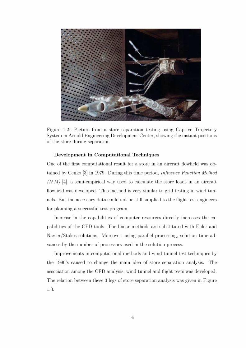
Figure 1.2: Picture from a store separation testing using Captive TrajectorySystem in Arnold Engineering Development Center, showing the instant positionsof the store during separation

Development in Computational Techniques

One of the first computational result for a store in an aircraft flowfield was ob-

tained by Cenko [3] in 1979. During this time period, Influence Function Method

(IFM) [4], a semi-empirical way used to calculate the store loads in an aircraft

flowfield was developed. This method is very similar to grid testing in wind tun-

nels. But the necessary data could not be still supplied to the flight test engineers

for planning a successful test program.

Increase in the capabilities of computer resources directly increases the ca-

pabilities of the CFD tools. The linear methods are substituted with Euler and

Navier/Stokes solutions. Moreover, using parallel processing, solution time ad-

vances by the number of processors used in the solution process.

Improvements in computational methods and wind tunnel test techniques by

the 1990’s caused to change the main idea of store separation analysis. The

association among the CFD analysis, wind tunnel and flight tests was developed.

The relation between these 3 legs of store separation analysis was given in Figure

1.3.

4

CFD ANALYSIS

FLIGHT TEST

WIND TUNNEL

V a l i d

a t e

a n a l

y s i s

R e d

u c e

F l i g

h t T

e s t

m a t

r i x

D e t e r m

i n e c r i t i c a l

c o n d i t i o n s

V a l i d a t e C

o d e

Validate W.T. Data

Plan Flight Test

Figure 1.3: Relation between CFD, wind tunnel and flight tests

CFD techniques have showed their capability in the store separation analysis

during the last decade of 20th century in three international CFD Challenges.

The results of these challenges have shown that CFD can match the wind tunnel

test data, and also the flight test results as well.

1.3 Literature Survey

The first store separation code used vortex lattice methods to model wing, and

sources and doublets to model the fuselage. It was developed by Nielsen Engi-

neering and Research Inc. (NEAR) [5] in 1971. The loads on the store are found

by using the slender body theory. Later, PAN AIR code [3] was developed in

1979, allowing a higher order linear calculation for complex aircraft/store combi-

nation even at transonic speeds. PAN AIR code was coupled with IFM and used

to find out the influence coefficients for the stores.

Advances in computer power and speed, and the solution techniques like

Chimera [6] approach and unstructured grid techniques [7], true CFD calcula-

tions of store trajectories became practical. These improvements led to three

CFD Challenges to determine how close CFD can come to matching wind tunnel

and flight test data.

First challenge was held in 1992. The configuration was the generic Wing-

5

Pylon-Finned Store [8]. The wind tunnel tests were performed in Arnold Engi-

neering Development Center (AEDC). Both Euler [9, 10] and thin layer Navier-

Stokes solutions [11] were in good agreement with the test data. A full potential

code, TranAir, [12] was also be able to get the similar results in a fraction of

time than the higher order codes. Today, these test data are still used for the

validation of CFD tools [13].

Second challenge was held in 1996 and named as Applied Computational Fluid

Dynamics (ACFD) Challenge I. The configuration was the F-16/Generic Finned

Store. Several codes were participated in this challenge. The fastest solution

is obtained by TranAir [14] code in 2 weeks time. The most accurate result

was obtained by OVERFLOW [15] solution, but this solution took 3 months of

time. SPLITFLOW [16] provided 24 number of solutions in four months of time,

some of which were in excellent agreement with the test data. The results were

tabulated and given in Table 1.1.

Table 1.1: Evaluation Results for ACFD Challenge I

TranAir SPLITFLOW USM3D OVERFLOW

Solution time 2 weeks 1 month 1 month 3 monthsAccuracy 3rd place 2nd place 3rd place 1st placeNumber of Solutions 8 24 8 1

After the flight tests of this configuration were performed, it was seen that

flight tests results did not match with the wind tunnel tests results.

The third CFD challenge was then announced as ACFD Challenge II. The

configuration was F-18/C with MK-84 JDAM. Both the flight and wind tunnel

test results were in good agreement with each other.

The results of several codes were in good agreement with the available test

data. The participating companies and their code were CFD Research Corpo-

ration (CFDRC) with CFD-FASTRAN flow solver, Air Force Wright Research

Laboratory with Cobalt flow solver and NAWSEP 6DOF motion module, Naval

Air Warfare Center with SPLITFLOW, USM3D and PUMA, and Lockheed Mar-

tin with SPLITFLOW.

6

Cobalt flow solver is a parallel, implicit, unstructured-grid Euler/Navier Stokes

code. Viscous solution of the F/A-18C aircraft solution consists of 6.62 million

cells (half-model for symmetry) including 4 million for the boundary layer. The

solution requires 10.1 GBytes of memory and the total 861 hours of CPU time

was needed for the solution using IBM SP2 processors.

USM3D code is a tetrahedral cell-centered, finite volume Euler and Navier-

Stokes flow solver. The viscous solution was run on a Cray C90 and required

315MW of memory and a total of 57.46 hours of CPU time.

SPLITFLOW is a cartesian-based, unstructured, adaptive Euler/Navier-Stokes

solver. The viscous solution was run on a Cray C90 requiring 256 MW of memory

and a total of 81.29 hours of CPU time.

Generally, the necessary accuracy was obtained, within the error range of wind

tunnel and flight tests. The interesting result of this challenge is that both Euler

and Navier/Stokes results gave similar results [17]. Comparisons of all the results

obtained at ACFD Challenge II were presented in [17].

1.4 Thesis Scope and Outline

The purpose of this study is to demonstrate some of the capabilities of the com-

putational prediction tools. Two separate computational tools are used; CFD-

FASTRAN, an inviscid Euler solver with chimera overlapping grid technique and

an unsteady panel method solver, USAERO, coupled with the integral boundary

layer method. These codes are used to obtain the unsteady trajectory characteris-

tics of a store released under subsonic flow conditions. The results are presented

in terms of store trajectory, angular orientations, forces acting on the store in

captive position and during separation process, and pressure distribution on the

store in captive position.

CFD-FASTRAN is one of the codes that use implicit Euler/Navier-Stokes

flow solver with chimera overlapping grid technique for relative body motion

problems. This code is validated for the generic wing-pylon-store test case once

and the results are presented in [18] and a similar technique of solution was further

used to validate the simulation of a jettisoned aircraft canopy trajectory in the

7

same reference. Separation results of JDAM from an F-18 fighter aircraft are also

published in [19].

USAERO, a time-stepping panel method coupled with a wake model and thin

boundary layer assumption with Flight Path Integrator (FPI) module, is the

other computational tool used for the present store separation problem. Since

the modeling and the solution time of a panel code is considerably less than that

of the Euler solutions, panel codes are frequently used as an engineering tool in

achieving practical objectives [20].

Two different wing-pylon-store configurations are solved. The first one is

the well-known generic wing-pylon-finned store test case [8]. It is solved with

the CFD-FASTRAN solver at a Mach of 0.95. There are several reports that

successfully predict the trajectory characteristics of this problem [21, 22, 23].

The results of the present computations are compared with the available exper-

imental and computational data. It is observed that all of the major trends of

the trajectory for this particular problem are captured with the present Euler

solution technique [24].

The next case is the same generic wing-pylon-store configuration solved at two

different Mach numbers of 0.3 and 0.6. Both codes are used to predict the c.g.

location and the orientations of the store in its trajectory. As a final case, the

separation of a fueltank from an F-16 fighter aircraft’s wing-pylon configuration

and from a full F-16 aircraft configuration are also demonstrated with the use of

USAERO unsteady panel code.

Unfortunately, no experimental data are available for Mach 0.3 and 0.6 cases of

both the generic wing-pylon-store and the fueltank separation from F-16 aircraft

cases for comparison purposes. However, it is believed that the present results

could be used to demonstrate the capabilities of both codes and their applicability

for store separation problem [25].

Chapter 1 of the thesis gives a brief description of store separation problem.

Historical background of store separation testing, wind-tunnel test techniques

and developments in computational methods are introduced in this chapter. A

literature survey about CFD tools used for store separation is also included.

8

Chapter 2 is about the theoretical background on which CFD-FASTRAN and

USAERO package programs are based. Governing equations together with the

boundary conditions modeling the fluid flow and their solution algorithms are

briefly mentioned.

The capabilities of the Euler solver is explained in Chapter 3. Grid genera-

tion, Chimera overset grid methodology and its use in store separation problem,

parallel processing, and 6-DOF motion model of CFD-FASTRAN are introduced.

Results of store alone and generic wing-pylon-store validation test cases with

the present method, that is, Euler solution with chimera overset grid technique

are given in Chapter 4.

Trajectory results of store separation from the generic wing-pylon-store and

F-16 fighter aircraft cases are given in Chapter 5. First case is solved with both

Euler and the unsteady panel codes. Similarities and differences in the results

are discussed. Second case is solved in wing alone and full aircraft configurations

using the unsteady panel code. Fuselage effect on the trajectory of the store after

separation is investigated.

Chapter 6 presents the conclusions about the present study.

9

CHAPTER 2

THEORETICAL BACKGROUND

2.1 Overview

Computational fluid dynamics has the advantage of analyzing the separation

phenomena with less time and cost than the experimental techniques. However,

accuracy of the solution depends on the flow model. Solution of a flowfield around

an aircraft with a turbulence modeling increases the accuracy of the solution by

considering the viscosity effects. But the number of unknowns needed to be solved

increases as well and are limited with the computational memory resources.

The challenge in separation analyses [2] is to decrease;

• man/hour required for modeling the problem,

• time required to obtain a solution,

and to increase

• accuracy of the solution

Modeling of the problem starts by importing the geometry from a CAD pro-

gram, continues with the construction of the computational domain or surface

paneling, and finalized by the start of the solution process. Time and man power

required for modeling depends not only on how much the man is skilled, but also

on the grid type that is used. For panel codes, only surface meshing is required.

For Euler solutions, structured, unstructured or hybrid grids can be used to con-

struct the solution domain. Navier/Stokes solutions require more attention to the

10

boundary layer around the wall boundaries. Therefore, time and skill required to

model a separation problem increases with the accuracy of the solution.

Time required to obtain a solution depends on

• the number of the unknowns to be solved,

• the methodology used in the solution of unknowns

• and the processor speeds of the computer resources.

The number of unknowns to be solved increases from panel codes to Navier/

Stokes solvers. Implicit methods converge faster than explicit methods. Increase

in processor speeds and the memory capacity of a single computer make it possible

to obtain solutions in shorter time.

Selection of the computational technique to be used in the solution of a store

separation problem depends on the how much of the flow physics needs to be

considered. If there is a strong interaction between the store and any part of the

aircraft with shocks, solution can be obtained with Euler or Navier/Stokes solvers

[26]. But higher order panel codes can also be used to get reasonably good results

in such complex problems [20].

Euler and panel solvers are widely used in external flow analysis as well as store

separation problems. Euler solvers are used instead of Navier/Stokes solvers when

viscous effects are negligible. Therefore Euler solutions take the advantage of less

memory requirements and less solution time when compared with Navier/Stokes

solutions.

Panel codes are used in the solution of incompressible potential flows, where

the flow is subsonic everywhere. Locally supersonic flows handled by Mach cor-

rection factors. Viscous effects can be added to the solution by boundary layer

coupling.

In this study, Euler solutions are used for flows at high Mach numbers and

where viscous effects can be neglected. For subsonic flows, unsteady panel code is

preferred, due to its fast turn-out time to obtain the solutions. Viscous effects are

also incorporated into the panel code calculations through an integral boundary

layer coupling.

11

Following sections briefly describes the governing equations, and their dis-

cretization in space and in time, and the boundary conditions that are used by

the Euler and the unsteady panel code.

2.2 CFD-FASTRAN Flow Solver

CFD-FASTRAN flow solver can handle a wide variety of physical phenomena

including compressible, viscous/inviscid/laminar/turbulent flows with steady or

time accurate calculations. Inviscid flow regime is governed by the Euler equations

whereas for the viscous flow solutions, Navier-Stokes equations are solved. Steady

state solutions take the advantage of numeric and advance the flow solution to

a typically faster final answer at the cost of losing the time accuracy. Time

accurate, unsteady solutions are required for the solution of transient flows such

as moving bodies.

Finite volume approach is used for the numerical integration of the discretized

governing equations, in which the flow domain is divided into discrete volumes.

Governing equations are solved for each cell and the flow information is stored at

the cell center. The flow from one cell to the next is determined by evaluating the

fluxes across the common faces. CFD-FASTRAN includes Roe’s Flux Difference

Splitting and Van Leer’s Flux Vector Splitting schemes for the flux calculations.

These schemes are spatially first order accurate and several slope limiters are

provided in CFD-FASTRAN which increases the spatial accuracy of the flux

schemes to second or third order.

2.2.1 Governing Equations

The fluid motion is governed by the time dependent Euler equations for an ideal

gas which expresses the conservation of mass, momentum and energy for a com-

pressible inviscid non-conducting adiabatic fluid in the absence of external forces.

The classical Euler equations are transformed for moving or deforming volumes

by Leibnitz’s Theorem. Conservation equations for an inviscid flow can be ma-

nipulated such that,

12

d

dt

∫

VQ dV +

∫

S(~Fc − Q~vg) · ~n dS = 0 (2.1)

where

Q =

ρ

ρu

ρv

ρw

e0

~Fc · ~n = ~V · ~n

ρ

ρu

ρv

ρw

e0 + p

+ p

0

nx

ny

nz

0

(2.2)

~vg is the volume surface velocity and it is taken as zero for non-moving body

problems. ~n is the unit vector normal to the control surface and nx, ny and nz

are the cartesian components of the surface unit normal.

These equations are closed by the equation of state, which for an ideal gas is

given by;

p = (γ − 1)(

e0 −1

2ρ

∣

∣

∣

~V∣

∣

∣

2)

(2.3)

where γ is the ration of specific heats and its value is 1.4 for air.

Equation 2.1 states that the time rate of change of the state vector Q within

the control volume V is balanced with the net convective flux ~Fc across the faces

of the volume.

2.2.2 Space and Time Discretization

The flux vector and the flux jacobians are evaluated using the idea of upwind

schemes. There are two upwinding flux schemes are available in CFD-FASTRAN.

The first scheme is based on Van Leer’s scheme and is considered to be a flux

vector splitting algorithm. Splitting the flux vector using this method make the

flux functions continuously differentiable at sonic and stagnation points. The

other approach is based on Roe’s approximate Riemann solver and is considered

as a flux difference scheme.

13

Roe’s scheme is considered to be non-monotone, which means that erroneous

extrema may be introduced into the flow solution, such as expansion shocks.

This difficulty can be removed by specifying entropy fix to increase the numerical

dissipation. On the other hand, Van Leer’s scheme is considered to be monotone

which means that dispersion (numerical oscillation) is unlikely to occur within

a flow near s strong gradient, such as a shock. However, Van Leer’s scheme is

more dissipative than Roe’s scheme in boundary layers which may cause if viscous

effects are highly important. Van Leer’s scheme’s dissipative effects also cause it

to be typically more robust than Roe’s scheme.

First order spatial accuracy is not suitable for many aerodynamic simulations,

especially if the flow is shock dominated as in transonic flows. Since both flux

schemes are first order spatially accurate, higher accuracy is obtained by using

flux limiters. Min-mod and Van Leer limiters, which are used in the present

calculations, provide second order spatial accuracy.

The solution for the discretized equation is achieved by a time marching algo-

rithm. For steady flows, the time marching scheme is repeated until the residuals

or the change in the solution variables fall below a tolerance level. The time

marching scheme produces a time-accurate answer for a transient simulation. In

steady calculations, local time stepping is used whereas a global time stepping is

used for the time accurate solutions.

A full implicit scheme is used for the present calculations. This scheme is

first order time accurate for the transient calculations. VanLeer’s and Roe’s flux

schemes are both used and tested for the calculations. It has been observed that

both methods give similar results in the present calculations.

2.2.3 Initial and Boundary Conditions

An initial condition is needed to start the solution process in all steady/unsteady

simulations. During steady state simulations of external flow problems, initial

conditions are only initial guesses and do not affect the final solution but the

convergence speed. Freestream values are assigned as initial conditions in the

entire domain. Unsteady, time accurate simulations are initialized by the steady

14

state solution of the same problem.

Inflow/Outflow BC is set at the farfield boundaries. This condition calculates

the total pressure and the total temperature from the user specified pressure,

temperature and velocities at the inflow boundaries. The velocity direction is

set by the user and the magnitude is determined by extrapolation from the inte-

rior domain. Same condition behaves as the fixed static pressure at the outflow

boundaries while the remaining flow variables are extrapolated from the interior

to the exit plane.

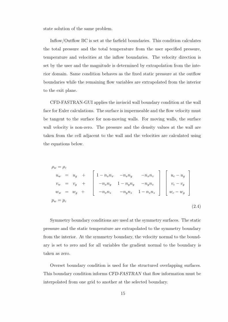
CFD-FASTRAN-GUI applies the inviscid wall boundary condition at the wall

face for Euler calculations. The surface is impermeable and the flow velocity must

be tangent to the surface for non-moving walls. For moving walls, the surface

wall velocity is non-zero. The pressure and the density values at the wall are

taken from the cell adjacent to the wall and the velocities are calculated using

the equations below.

ρw = ρc

uw = ug +

vw = vg +

ww = wg +

1 − nxnx −nxny −nxnz

−nxny 1 − nyny −nynz

−nxnz −nynz 1 − nznz

uc − ug

vc − vg

wc − wg

pw = pc

(2.4)

Symmetry boundary conditions are used at the symmetry surfaces. The static

pressure and the static temperature are extrapolated to the symmetry boundary

from the interior. At the symmetry boundary, the velocity normal to the bound-

ary is set to zero and for all variables the gradient normal to the boundary is

taken as zero.

Overset boundary condition is used for the structured overlapping surfaces.

This boundary condition informs CFD-FASTRAN that flow information must be

interpolated from one grid to another at the selected boundary.

15

2.3 USAERO Panel Code

USAERO is a low order panel code, which uses a time-stepping approach in the

calculation of non-dimensional surface pressure coefficient and wake convection.

The surface of the model is discretized with quadrilateral panels.

The basis of the method is that, the surface singularity model which uses

quadrilateral panels of uniformly distributed doublets and sources are calculated

at each time step. The surface integrals in Green’s theorem are evaluated in a

piece wise manner over each panel to form panel influence coefficients. These are

evaluated for each panel acting at the central control points on all the surface

panels, thus forming a matrix of influence coefficients. Usually the source values

are determined at the start of each time step according to the local velocity

component normal to the panel surface. The doublet values are then solved

using the matrix equations.

The tangential velocity at the solid surfaces of the configuration is obtained

from the doublet gradient. The normal component is provided by the source

value. Off-body velocity perturbations are evaluated by summing all doublet and

source singularity contributions. These velocities are used for general flow field

information as well as for wake point convection. The wakes grow with each time

step, with new wake points being propagated from the wake-shedding lines, while

all the previous wake points are convected at the local fluid velocity.

2.3.1 Governing Equations

For an inviscid, irrotational and incompressible flow, Laplace equation can be

written as;

∇2φ = 0 (2.5)

The convention adopted here is that the perturbation velocity, ~v, is the neg-

ative gradient of φ;

~v = −~∇φ (2.6)

Green’s Theorem is applied in the solution procedure of Equation 2.5. The

contributions for the velocity potential, φp, for a point P on the wetted side of

16

the surface, are assumed to be due to;

• a surface distribution of normal doublets

• a surface distribution of sources

• the vortex shedding along the wake.

The source distribution is determined applying the Neumann boundary con-

dition specifying the resultant normal velocity at the wall boundary. As for the

wake treatment, the wake vorticity effectively varies in time and space according

to the local stretching or contraction of the wake sheet as the wake points convect

at the local velocities. Once source distribution and vortex shedding is known,

doublet distribution along the surface is computed through the solution of Eqn.

2.5. Finally, perturbation velocity ~v is calculated using Eqn. 2.6 knowing φ.

2.3.2 Wall Boundry Conditions

The condition to be satisfied on the wall boundary is that the normal com-

ponent of the velocity to the wall equals to zero unless it is specified with an

inflow/outflow normal velocity definition and/or boundary layer displacement

effect. The normal component of the panel velocity includes the perturbation

velocity from Equation 2.6, and the surface velocity relative to the undisturbed

fluid. The surface velocity ~Vs is defined as given in Equation 2.7.

~Vs = ~Vb + ~Ω × ~R − ~V∞ (2.7)

First term is coming from the translational velocity of the body, the second

term is from the rotational velocity of the body and the last term is from the

uniform flow.

2.3.3 Surface Pressure Calculation

The pressure coefficient is evaluated at each panel center using the Bernoulli

equation for a moving frame given in Eqn. 2.8.

Cp = V 2

s − V 2 + 2

(

δφ

δτ

)

(2.8)

17

Vs is the surface point velocity and V is the total fluid velocity relative to

the surface point. The third term in the equation is evaluated by using simple

differencing relative to the previous time step.

2.3.4 Wake Treatment

There is only one wake type to be used in USAERO, which convects with the

local flow velocity. Internal treatment to the wake type is done automatically by

the code through the boundary condition at the separation line. Also the jump

in total pressure across a closed vortex-tube wake (jets or separation wake) is

obtained automatically through the δφ/δτ term in the pressure equation. In ad-

dition, this jump in total pressure is sensed automatically by any object enclosed

by the tube.

18

CHAPTER 3

FLOW SOLVER

3.1 Overview

CFD-FASTRAN flow solver is a CFD package tool which includes its own pre

and post-processors, CFD-GEOM and CFD-VIEW, respectively. CFD-GEOM

is used in the creation of the geometry from points, lines, curves and surfaces.

The same pre-processor is used for the generation of the structured grid. Chimera

grids are created independently from each other using CFD-GEOM. Merging and

overlapping the chimera grids are accomplished by a simple cut-paste technique.

Hole-cutting process is performed automatically by the code during the solution

state.

Parallel execution capability is applicable using both structured and unstruc-

tured grids and available only in Linux operating systems. CFD-FASTRAN uses

a domain decomposition method based on multi-block approach in structured

grids. In this decomposition, each block or blocks is/are assigned to different

processor(s). Therefore, in order to have equal load distribution on processors,

the blocks must be on same size of order. 6DOF module is used in store separa-

tion applications. Necessary data is input by the user using the Graphical User

Interface (GUI). Application of the 6DOF module starts by entering the origin

coordinates of the new body coordinate system. The forces acting on the store

is selected at this stage. Available force features are aerodynamic, point, thrust

19

and gravitational forces. If needed, any prescribed motion can be modelled using

the module.

Following sections briefly describes these features used in the solution of a

store separation problem in CFD-FASTRAN.

3.2 Geometry Creation

The entire grid used in the solution process is generated with the pre-processor of

CFD-FASTRAN, which is called CFD-GEOM. This tool can be used to generate

structured, unstructured and also hybrid grids. In this study, structured grid

tools of CFD-GEOM are used since CFD-FASTRAN solver use the body motion

capability with chimera overlapping structured grids only.

The surface definition of the geometries is also generated using the same pre-

processor. Given airfoil section defined by points on the line segments can be im-

ported to the CFD-GEOM. Scaling property is used to scale the non-dimensional

chord to the real values in meters. The root section of the wing is extruded

along the span using the extrusion property in order to create the wing surface

geometry. The store geometry is created by revolving the boundary curve that

defines the surface curvature, around its axis of rotation. Other properties such

as split, project, trim, translate, rotate are also used in the creation of the related

geometries.

If necessary, any CAD file given in IGES or Plot3D format could also be im-

ported by the pre-processor, which might speed up the geometry creation process.

In this study, the geometry of wing-pylon-store configuration is created using

CFD-GEOM.

3.3 Structured Grid Generation

The structured grid generation process starts by defining the grid point number

and its distribution on lines or curves. Edge creation option is used for this

purpose. CFD-GEOM supports uniform, exponential and hyperbolic tangent grid

point distribution along edges. Rectangular surface mesh of interest is defined

20

by three or four edges using face creation option. Revolving an edge around its

axis of rotation can be used to create surface mesh of a circular body. Any face

grid created can be projected exactly onto any NURBS surface set by projection.

The projection algorithm projects the grid points to the nearest location on the

NURBS surface to that grid point.

Six face sets combine to form a block. A block can be constructed manually by

specifying six face sets that comprise the Imin, Imax, Jmin, Jmax, Kmin, Kmax

sides of the block or by extruding a face. Creating a block means constructing

the computational domain.

It is difficult to create the computational domain for complex geometries using

single block. Therefore, a multi-zonal approach where the physical flow domain

is divided into a number of geometrically simple sub-domains (zones) is highly

favored over the single-zone counterpart. The multi-zonal approach also has the

advantage that the mesh in a certain zone of the flow domain can be easily refined

to accurately resolve shocks without modifying the meshes in the neighboring

zones. Furthermore, multi zonal approach is needed for solving problems using

multi-processing parallel computers in CFD-FASTRAN. In this study, structured

grids with multi-block approach are used in creating the computational domains.

3.4 CHIMERA Methodology

There are two different multi-zonal algorithms depending on whether zonal bound-

aries exactly match or arbitrarily intersect each other. The former is named

patched grid approach and the latter the Overset grid (Chimera) approach. In

this study, both approaches are used.

In Chimera, overset grids can move relative to each other without disturbing

the grids in other zones. Since different zones are not required to align with each

other, zonal grids can then be produced completely independently.

Some advantages and disadvantages of the patched and overset grid algorithms

are summarized below [27]:

Patched grid scheme

• Fully conservative

21

• Interpolation from one zone to another zone is unnecessary

• Zonal interfaces need perfect match

Overset grid scheme

• Arbitrary boundary interface matches

• Grids can move relative to each other

• Zonal boundary treatment is not fully conservative

• Two-way interpolations are required

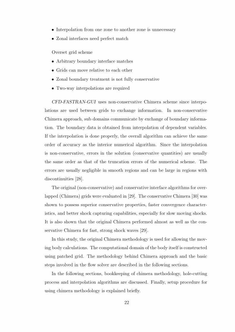
CFD-FASTRAN-GUI uses non-conservative Chimera scheme since interpo-

lations are used between grids to exchange information. In non-conservative

Chimera approach, sub domains communicate by exchange of boundary informa-

tion. The boundary data is obtained from interpolation of dependent variables.

If the interpolation is done properly, the overall algorithm can achieve the same

order of accuracy as the interior numerical algorithm. Since the interpolation

is non-conservative, errors in the solution (conservative quantities) are usually

the same order as that of the truncation errors of the numerical scheme. The

errors are usually negligible in smooth regions and can be large in regions with

discontinuities [28].

The original (non-conservative) and conservative interface algorithms for over-

lapped (Chimera) grids were evaluated in [29]. The conservative Chimera [30] was

shown to possess superior conservative properties, faster convergence character-

istics, and better shock capturing capabilities, especially for slow moving shocks.

It is also shown that the original Chimera performed almost as well as the con-

servative Chimera for fast, strong shock waves [29].

In this study, the original Chimera methodology is used for allowing the mov-

ing body calculations. The computational domain of the body itself is constructed

using patched grid. The methodology behind Chimera approach and the basic

steps involved in the flow solver are described in the following sections.

In the following sections, bookkeeping of chimera methodology, hole-cutting

process and interpolation algorithms are discussed. Finally, setup procedure for

using chimera methodology is explained briefly.

22

3.4.1 Searching Process

Chimera scheme used by CFD-FASTRAN can find out the overlapping cells of

different domains automatically. This property involves frequent searches over

the cells in different zones. This searching process is optimized by an Alternating

Digital Tree (ADT) [31]. AD tree disseminates the cells of a grid in a tree based

structure, based on certain data such as the coordinates of cell centroid and the

coordinates of bounding box for a cell which is a point in 6D space [31].

3.4.2 Hole-Cutting Process

Hole-cutting is the process of blanking the cells in each zone that overlap with a

wall boundary from another zone overset. Identification of the chimera-boundary

cells, which are used to interpolate the flow variables from one zone to the other

overlapping zones are also performed in this stage.

Major Zone is referred to the zone in which cells are blanked and Minor Zone

is the zone which contains the wall boundary.

If there is wall a boundary in both overlapping zones, each zone is a major and

a minor zone at the same time. The cells in the major zone that intersects wall

boundary faces of the minor zone are first identified. This procedure is performed

using the AD tree.

If the edge intersects a wall boundary, then the point at which they intersect

is found. Next step is to find out if the nodes of the edge are inside or outside the

wall boundary. The cell is marked as cut-cell if one of the edge nodes is outside

the wall boundary while the other is inside.

After determining the cut-cells, the nodes of the major zone that lie inside the

blanket of these cut-cells are marked. These cells are blanked-out in the major

zone. The region of blanked cells, inclusive of the cut-cells, is referred as chimera

hole. The cells of the major zone surrounding the chimera-hole are marked as

chimera-boundary cells. The solution is interpolated to these chimera bound-

ary cells from the underlying donor cells in the minor zone. The mathematical

expressions for this search process are given in Ref. [31].

23

(a) Overlapping wall boundaries of the wing

(b) Chimera hole (grey color), buffer layer (boldgrey)

(c) Hole in the store domain

Figure 3.1: Steps of hole-cutting process for wall boundaries of wing in the storedomain, sectional cut through store center in 3D

Buffer layer is an additional layer of blanked-cells added to the chimera-hole.

If more than one buffer layer is used, the interpolation of flow variables to the

major zone is performed using the cells which are number of buffer layer times

away from the wall boundary of the minor zone. This prevents the major zone

24

from receiving flow information too close to the wall surface.

In order to perform an interpolation using more than one cell layer in the

minor zone, additional Fringe Layers are used.

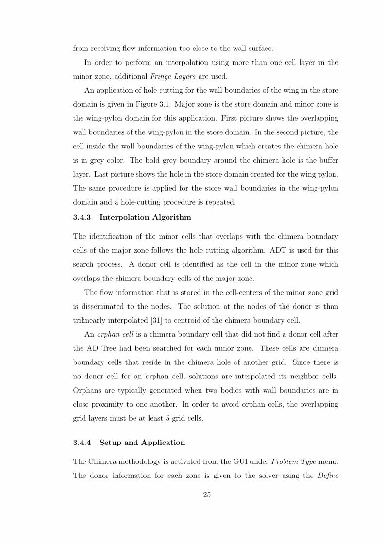
An application of hole-cutting for the wall boundaries of the wing in the store

domain is given in Figure 3.1. Major zone is the store domain and minor zone is

the wing-pylon domain for this application. First picture shows the overlapping

wall boundaries of the wing-pylon in the store domain. In the second picture, the

cell inside the wall boundaries of the wing-pylon which creates the chimera hole

is in grey color. The bold grey boundary around the chimera hole is the buffer

layer. Last picture shows the hole in the store domain created for the wing-pylon.

The same procedure is applied for the store wall boundaries in the wing-pylon

domain and a hole-cutting procedure is repeated.

3.4.3 Interpolation Algorithm

The identification of the minor cells that overlaps with the chimera boundary

cells of the major zone follows the hole-cutting algorithm. ADT is used for this

search process. A donor cell is identified as the cell in the minor zone which

overlaps the chimera boundary cells of the major zone.

The flow information that is stored in the cell-centers of the minor zone grid

is disseminated to the nodes. The solution at the nodes of the donor is than

trilinearly interpolated [31] to centroid of the chimera boundary cell.

An orphan cell is a chimera boundary cell that did not find a donor cell after

the AD Tree had been searched for each minor zone. These cells are chimera

boundary cells that reside in the chimera hole of another grid. Since there is

no donor cell for an orphan cell, solutions are interpolated its neighbor cells.

Orphans are typically generated when two bodies with wall boundaries are in

close proximity to one another. In order to avoid orphan cells, the overlapping

grid layers must be at least 5 grid cells.

3.4.4 Setup and Application

The Chimera methodology is activated from the GUI under Problem Type menu.

The donor information for each zone is given to the solver using the Define

25

Chimera sub-menu under Model Options page. If a zone is not overlapping with

any other zones, this is also declared to the solver. All of these information speeds

up the identification process of the chimera boundary cells. If the geometry is

too complex in order to identify if a zone is overlapping with another zone or not,

all of the zones can be taken as candidate donor zone, excluding the ones that

are in the same domain.

Chimera Stencil Search Cycles controls the chimera hole-cutting frequency.

For steady problems hole-cutting is performed only once and the frequency is

ignored. For unsteady time accurate problems, depending on the displacements

and time step size, this frequency is chosen between 10 and 20. In this study,

this value is taken as 10. Therefore after every 10 time steps, solver searches for

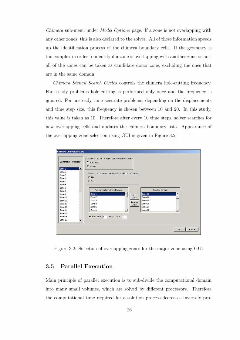
new overlapping cells and updates the chimera boundary lists. Appearance of

the overlapping zone selection using GUI is given in Figure 3.2

Figure 3.2: Selection of overlapping zones for the major zone using GUI

3.5 Parallel Execution

Main principle of parallel execution is to sub-divide the computational domain

into many small volumes, which are solved by different processors. Therefore

the computational time required for a solution process decreases inversely pro-

26

portional to the number of processors used. The necessary coupling between the

solutions in the different sub-domains is accomplished by appropriate transfers of

data between the processors. The data transfer speed affects the computational

time required for the solution. For example, the time required for a four proces-

sor job will always be more slightly more than 1/4th of the time required for the

same job to be solved by a single processor. The structured-grid solver uses the

Multi-Disciplinary Computing Environment (MDICE) utility to accomplish the

data transfers between the CPU’s. MDICE is a library of functions, developed

by CFDRC, for storing data in arrays or other data-structures and is used for

transferring or interpolating this data between different, simultaneously-running,

arbitrarily-different codes, and for synchronizing the necessary data copying and

data transfer operations [31]. MDICE also has several capabilities related to

automated chimera hole-cutting and interpolation.

The CFD-FASTRAN structured-grid solver does not break a domain into sub-

domains automatically. The domain decomposition is performed by distributing

the blocks (zones) to different processors. The number of processors that can be

used is limited with the number of zones used to construct the computational

domain. The blocks must be created nearly of the same size in order to obtain a

well balanced, equal load distribution.

3.5.1 Setup and Application Process

Parallel execution setup can be done using the CFD-FASTRAN-GUI. The pro-

cessors, which are going to be used in the parallel execution, are initially listed in

the fastran.hosts file created under the home directory of the user. This file also

includes the relative speeds of the processors. Using the GUI, under parallel set

up menu, these names can be found out. The blocks are distributed by the GUI

after the processors are chosen. This distribution is optimized for the best per-

formance depending on the speed of the processors and the block sizes. However,

user can redistribute the blocks to the processors manually. The first processor

becomes the master of the cluster, which performs the merging of solution files

at the end of the computations. If chimera overlapping grids are used for the

27

computations, the last processor is assigned as the Chimera host, which performs

the chimera related applications only.

Initial registry of the parallel execution is done by execution of mdicer program

in any of the nodes used in the computations. The registry name given out by the

program after this execution is used for starting the mdice daemons at the other

nodes of the cluster. The parallel solution is started from the command-line. The

decomposed domains are merged automatically at the end of the solution process.

3.6 Moving Body Module and 6DOF Equations

One of the capabilities of CFD-FASTRAN solver that is used for this study is

the moving body module. This module is used for unsteady and time accurate

problems such as store separation. This capability requires the rigidity of the

body and the grids of the moving body being structured type. The motion of

the body can be determined by a six degree of freedom calculation or it can be

prescribed by the user.

The six degree of freedom, 6DOF, routine is based on the fluid flow solution

in CFD-FASTRAN. Pressures and shear stresses are used to determine forces

and moments acting on the body. In turn, these forces and moments are used

in the general equations of motion to calculate translational and rotational dis-

placements of the body.

The equations of motion for a rigid body with constant mass and mass mo-

ments of inertia are solved in order to obtain the linear and angular velocities

and the displacements of the body in a delta time step size. These equations are

given below.

~F = md~v

dt(3.1)

~M =∂~h

∂t+ ~ω × ~h (3.2)

where m is the body mass, ~v is the linear velocity of the center of gravity, ~h is

the angular momentum, ~ω is angular velocity about the body’s center of gravity.

28

INITIAL STATE

Initial Linear and Angular Velocities, t=0

CFD-FASTRANUnsteady solution at time t

Integration of Forces

V t+∆t=V t+∆t (Ft+∆t /m)→→ →→

Integration of Moments

ht+∆t=ht+∆t (M t+∆t - w x h)→→ → →

Linear Displacements

∆Rt+∆t=(V t+ V t+∆t)∆t /2

→→ →

wt+∆t=I x h t+∆t

Angular Displacements

∆θt+∆t=(wt+ wt+∆t)∆t /2

New Oriantation ofthe Moving Body

→

t=t+∆t

Modified Geometrywith Chimera grid

→→

→→→→→

∼

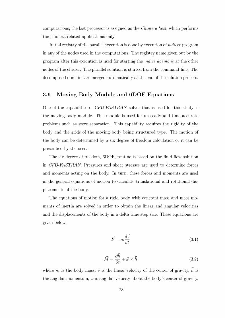
Figure 3.3: Coupling 6DOF calculations with the flow solver using Moving BodyModule

The force equation Eqn.3.1 is in the inertial frame of reference. The momen-

tum equation Eqn.3.2 is in the body fixed frame of reference. The moments of

inertia are completely based on the body rotating about an axis passing through

its center of gravity.

The main essential steps involved in these computations are given in Figure

3.3. This figure also summaries the coupling steps of the flow solver with the

6DOF module.

3.7 Output Data

A file is created named ORPHAN, which prints out lists the cells which do not

have valid interpolation stencils. The list includes the zone number, cell indices,

and (x, y, z) location of the cell centroid.

29

The model.DYNA and model.DYNB files contain force and moment data cre-

ated by each motion model. At each cycle, model.DYNA contains the individual

forces in the x, y, and z directions. The individual forces printed in the file depend

on the options selected in the GUI. The model.DYNB file lists the total forces in

the x, y, and z directions for both inertial and body fixed axes. The total mo-

ments taken about the inertial (0, 0, 0) are also listed in inertial and body fixed

axes. In model.KINA, the position, linear velocity and linear acceleration of the

center of gravity of a motion model are printed out for each cycle. In model.KINB

file, inertial angular displacement, body-fixed angular displacement, body-fixed

angular velocity and body-fixed angular acceleration quantities are printed out

for the motion model.

30

CHAPTER 4

FLOW SOLVER VALIDATION TEST CASES

4.1 Overview

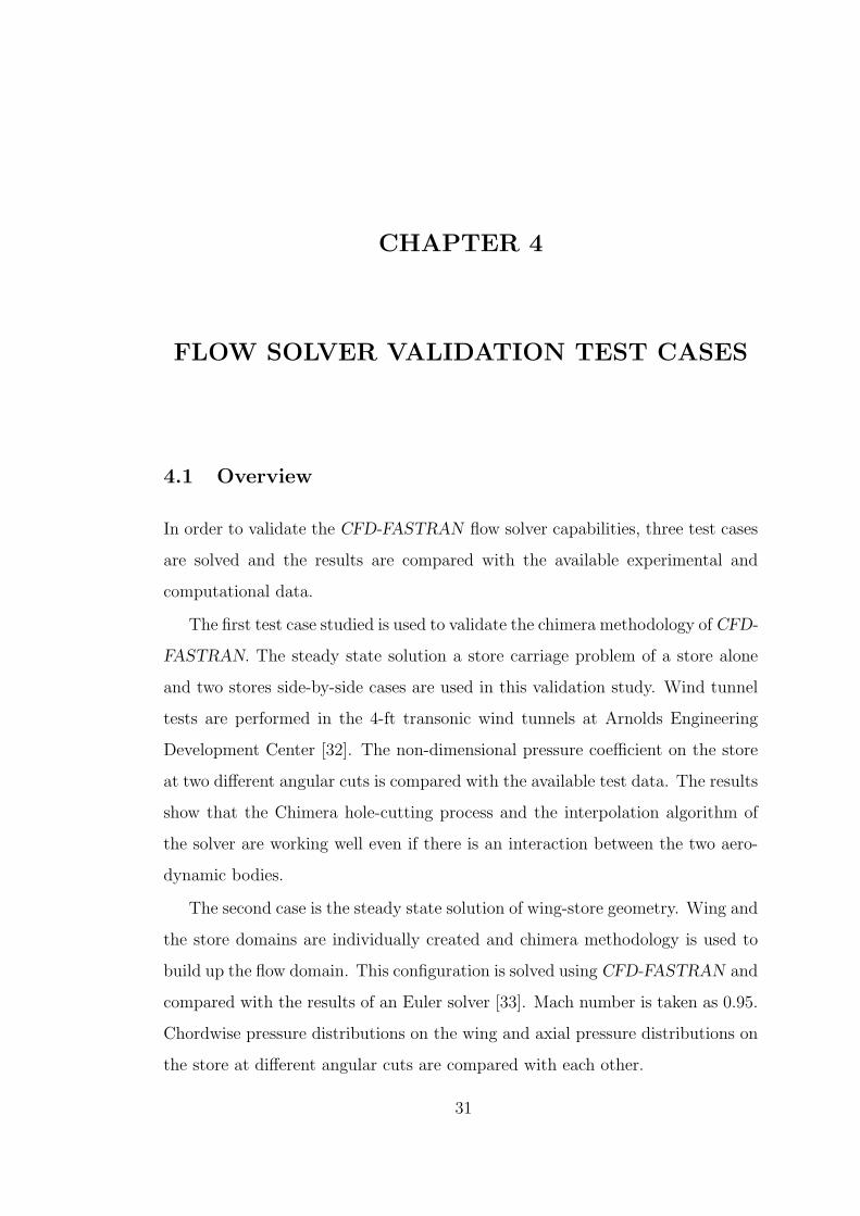
In order to validate the CFD-FASTRAN flow solver capabilities, three test cases

are solved and the results are compared with the available experimental and

computational data.

The first test case studied is used to validate the chimera methodology of CFD-

FASTRAN. The steady state solution a store carriage problem of a store alone

and two stores side-by-side cases are used in this validation study. Wind tunnel

tests are performed in the 4-ft transonic wind tunnels at Arnolds Engineering

Development Center [32]. The non-dimensional pressure coefficient on the store

at two different angular cuts is compared with the available test data. The results

show that the Chimera hole-cutting process and the interpolation algorithm of

the solver are working well even if there is an interaction between the two aero-

dynamic bodies.

The second case is the steady state solution of wing-store geometry. Wing and

the store domains are individually created and chimera methodology is used to

build up the flow domain. This configuration is solved using CFD-FASTRAN and

compared with the results of an Euler solver [33]. Mach number is taken as 0.95.

Chordwise pressure distributions on the wing and axial pressure distributions on

the store at different angular cuts are compared with each other.

31

The third one is the validation of a store separation test case. The generic

wing-pylon-store configuration is used for this study. The wind tunnel tests per-

formed at Arnold Engineering Development Center’s (AEDC) 4-Foot Transonic

Aerodynamic Wind Tunnel [8]. Test data are collected at store’s carriage position

and at selected points along the trajectory of the store. Captive Trajectory

System (CTS) simulated the motion of the store motion. The test data includes

dimensionless pressure coefficient distribution on store, and force and moment

coefficients acting on the store in its trajectory.

4.2 Chimera Validation Test Cases

The store used in the separation analysis is used to validate the chimera inter-

polation algorithm of CFD-FASTRAN. Two cases are considered for this study;

store alone and two stores side by side. The experimental data are available in

[32].

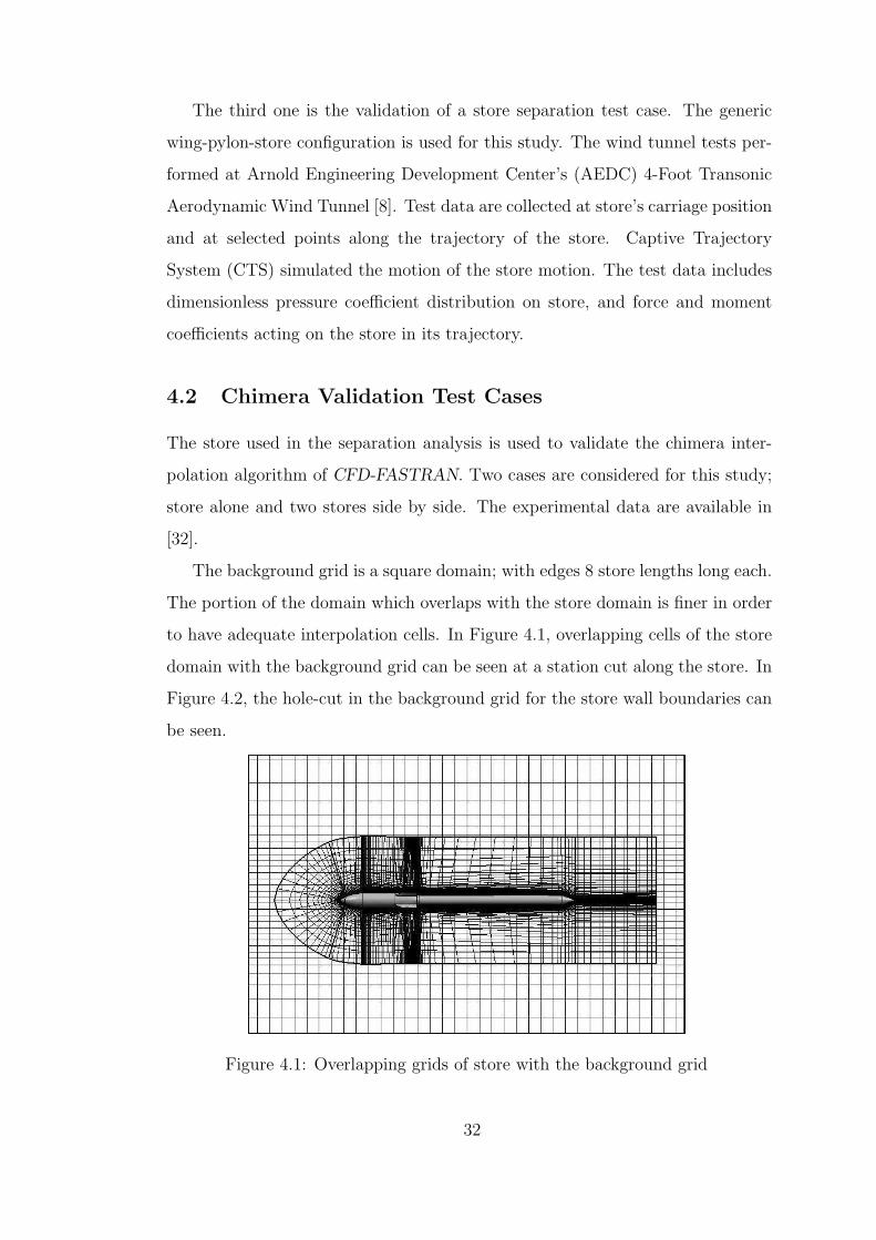
The background grid is a square domain; with edges 8 store lengths long each.

The portion of the domain which overlaps with the store domain is finer in order

to have adequate interpolation cells. In Figure 4.1, overlapping cells of the store

domain with the background grid can be seen at a station cut along the store. In

Figure 4.2, the hole-cut in the background grid for the store wall boundaries can

be seen.

Figure 4.1: Overlapping grids of store with the background grid

32

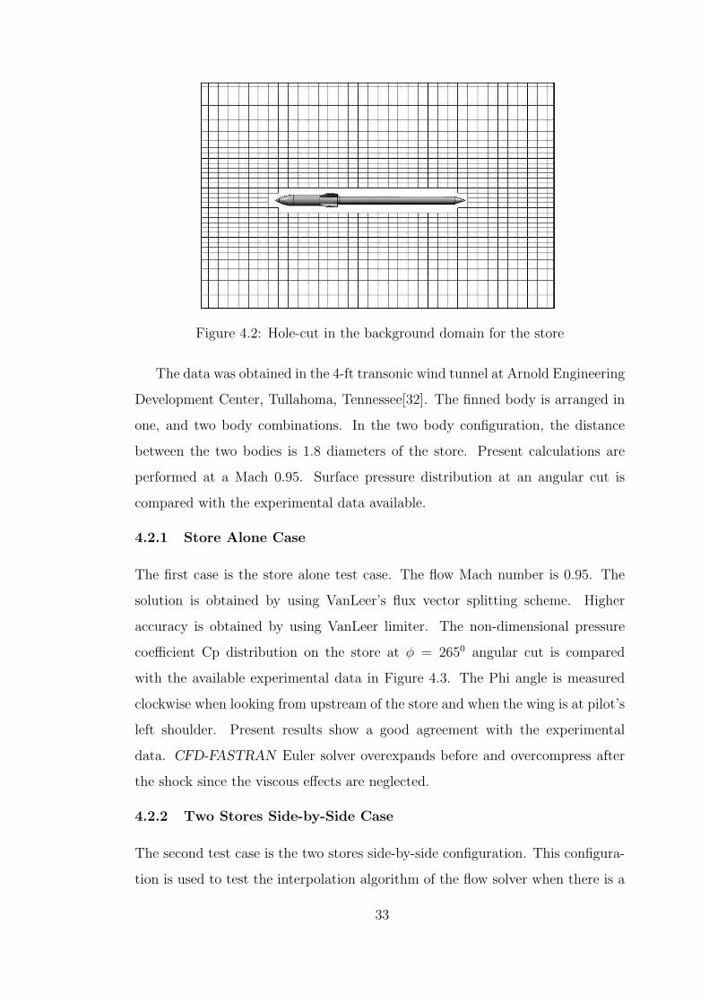
Figure 4.2: Hole-cut in the background domain for the store

The data was obtained in the 4-ft transonic wind tunnel at Arnold Engineering

Development Center, Tullahoma, Tennessee[32]. The finned body is arranged in

one, and two body combinations. In the two body configuration, the distance

between the two bodies is 1.8 diameters of the store. Present calculations are

performed at a Mach 0.95. Surface pressure distribution at an angular cut is

compared with the experimental data available.

4.2.1 Store Alone Case

The first case is the store alone test case. The flow Mach number is 0.95. The

solution is obtained by using VanLeer’s flux vector splitting scheme. Higher

accuracy is obtained by using VanLeer limiter. The non-dimensional pressure

coefficient Cp distribution on the store at φ = 2650 angular cut is compared

with the available experimental data in Figure 4.3. The Phi angle is measured

clockwise when looking from upstream of the store and when the wing is at pilot’s

left shoulder. Present results show a good agreement with the experimental

data. CFD-FASTRAN Euler solver overexpands before and overcompress after

the shock since the viscous effects are neglected.

4.2.2 Two Stores Side-by-Side Case

The second test case is the two stores side-by-side configuration. This configura-

tion is used to test the interpolation algorithm of the flow solver when there is a

33

X/L

Pre

ssur

eC

oeff

icie

ntC

p

0 0.25 0.5 0.75 1

-1

-0.75

-0.5

-0.25

0

0.25

0.5

0.75

1

EXP. DATA - (one store)CFD-FASTRAN (one store)

Mach 0.95 Phi=265 deg

Figure 4.3: Comparison of pressure coefficient distribution on the store withexperimental data [32], one store configuration, M=0.95

strong interaction between two wall boundaries. The distance between the stores

is 1.8 diameters of the store body. The interpolation between the two domains

and the background grid is realized by using the chimera boundary cells. A cut

through the fins shows the overlapping grids of the two stores in Figure 4.4.

The non-dimensional pressure coefficient Cp distribution on the right store

while looking from upstream at φ = 2650 angular cut is compared with the

available experimental data in Figure 4.5. It is expected that the flow accelerates

between the two bodies, as it is identified by the increase in expansion peaks. Also

Figure 4.4: Overlapping grids and hole-cutting through a section

34

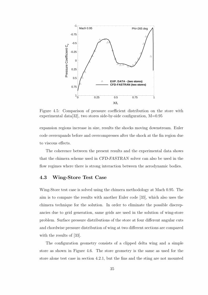
X/L

Pre

ssur

eC

oeff

icie

ntC

p

0 0.25 0.5 0.75 1

-1

-0.75

-0.5

-0.25

0

0.25

0.5

0.75

1

EXP. DATA - (two stores)CFD-FASTRAN (two stores)

Mach 0.95 Phi=265 deg

Figure 4.5: Comparison of pressure coefficient distribution on the store withexperimental data[32], two stores side-by-side configuration, M=0.95

expansion regions increase in size, results the shocks moving downstream. Euler

code overexpands before and overcompresses after the shock at the fin region due

to viscous effects.

The coherence between the present results and the experimental data shows

that the chimera scheme used in CFD-FASTRAN solver can also be used in the

flow regimes where there is strong interaction between the aerodynamic bodies.

4.3 Wing-Store Test Case

Wing-Store test case is solved using the chimera methodology at Mach 0.95. The

aim is to compare the results with another Euler code [33], which also uses the

chimera technique for the solution. In order to eliminate the possible discrep-

ancies due to grid generation, same grids are used in the solution of wing-store

problem. Surface pressure distributions of the store at four different angular cuts

and chordwise pressure distribution of wing at two different sections are compared

with the results of [33].

The configuration geometry consists of a clipped delta wing and a simple

store as shown in Figure 4.6. The store geometry is the same as used for the

store alone test case in section 4.2.1, but the fins and the sting are not mounted

35

Figure 4.6: Mesh view for the wing-store configuration [33]

on the store for the ease of grid generation. The wing geometry is also used in

the store separation test case and will be described in Section 4.4.1.1.

C-H type grid is used for the wing and a total number of 958, 000 cells are

produced for the solution domain. O type grid is used for the store. Total number

of 124,000 cells are produced for the store domain. The wing grid is generated by

CFD-GEOM, whereas the store grid is generated by the algebraic grid generation

techniques [33].

An implicit time integration method with Van-Leer flux splitting scheme is

used by CFD-FASTRAN solver. 900 iterations are needed to reach a converged

solution. CFL number is taken as 20 for the calculations. The other Euler solver

uses a finite difference method with an implicit time integration scheme. 6300

iterations are needed for a converged solution. Memory and CPU comparisons

between the two solvers are given in Table 4.1

Table 4.1: Memory need and CPU time comparisons of CFD-FASTRAN andEuler Solver[33]

Solver Processor CPU time Req. Mem.

CFD-FASTRAN 1 40 hrs. 936 MBEuler Solver 2 20 hrs. 280 MB

36

x/L

Cp

0.0 0.2 0.4 0.6 0.8 1.0

-1.0

-0.5

0.0

0.5

1.0

Euler Sol. [33]CFD-FASTRAN

Phi = 0 deg.Store

(a) φ = 0o

x/L

Cp

0.0 0.2 0.4 0.6 0.8 1.0

-1.0

-0.5

0.0

0.5

1.0

Euler Sol. [33]CFD-FASTRAN

Phi = 90 deg.Store

(b) φ = 90o

x/L

Cp

0.0 0.2 0.4 0.6 0.8 1.0

-1.0

-0.5

0.0

0.5

1.0

Euler Sol. [33]CFD-FASTRAN

Phi = 180 deg.Store

(c) φ = 180o

x/L

Cp

0.0 0.2 0.4 0.6 0.8 1.0

-1.0

-0.5

0.0

0.5

1.0

Euler Sol. [33]CFD-FASTRAN

Phi = 270 deg.Store

(d) φ = 270o

Figure 4.7: Pressure distributions on the store and comparison to [33]

The pressure distribution on the store along the axial direction at four different

phi angles are given in Figure 4.7.

The pressure coefficient distributions obtained by the two codes are almost the

same with small differences in the magnitudes. Smoother passages after the first

shock are observed in the Euler code [33] solution results due to artificial viscosity

effects. The far most location of the store from the wing, φ = 1800 angular cut

has shown the best similarity between the two codes. At x = 0.25, both codes

has shown the compression at all angles. But at φ = 00 and φ = 2700 angular

cuts, this compression has a higher strength in the results of CFD-FASTRAN.

37

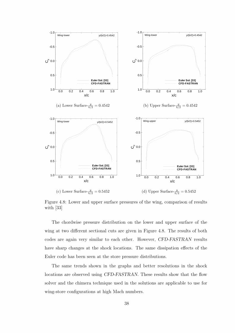
x/c

Cp

0.0 0.2 0.4 0.6 0.8 1.0

-1.0

-0.5

0.0

0.5

1.0

Euler Sol. [33]CFD-FASTRAN

y/(b/2)=0.4542Wing-lower

(a) Lower Surface- yb/2

= 0.4542

x/c

Cp

0.0 0.2 0.4 0.6 0.8 1.0

-1.0

-0.5

0.0

0.5

1.0

Euler Sol. [33]CFD-FASTRAN

y/(b/2)=0.4542Wing-lower

(b) Upper Surface- yb/2

= 0.4542

x/c

Cp

0.0 0.2 0.4 0.6 0.8 1.0

-1.0

-0.5

0.0

0.5

1.0

Euler Sol. [33]CFD-FASTRAN

y/(b/2)=0.5452Wing-lower

(c) Lower Surface- yb/2

= 0.5452

x/c

Cp

0.0 0.2 0.4 0.6 0.8 1.0

-1.0

-0.5

0.0

0.5

1.0

Euler Sol. [33]CFD-FASTRAN

y/(b/2)=0.5452Wing-upper

(d) Upper Surface- yb/2

= 0.5452

Figure 4.8: Lower and upper surface pressures of the wing, comparison of resultswith [33]

The chordwise pressure distribution on the lower and upper surface of the

wing at two different sectional cuts are given in Figure 4.8. The results of both

codes are again very similar to each other. However, CFD-FASTRAN results

have sharp changes at the shock locations. The same dissipation effects of the

Euler code has been seen at the store pressure distributions.

The same trends shown in the graphs and better resolutions in the shock

locations are observed using CFD-FASTRAN. These results show that the flow

solver and the chimera technique used in the solutions are applicable to use for

wing-store configurations at high Mach numbers.

38

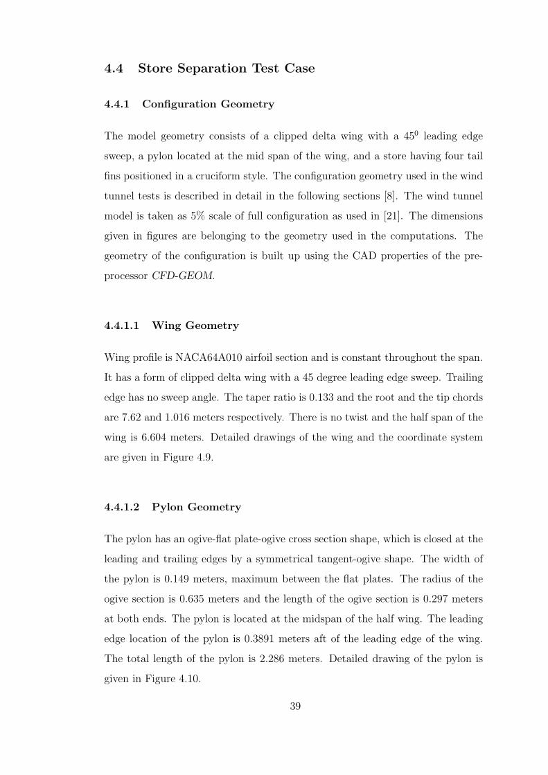
4.4 Store Separation Test Case

4.4.1 Configuration Geometry

The model geometry consists of a clipped delta wing with a 450 leading edge

sweep, a pylon located at the mid span of the wing, and a store having four tail

fins positioned in a cruciform style. The configuration geometry used in the wind

tunnel tests is described in detail in the following sections [8]. The wind tunnel

model is taken as 5% scale of full configuration as used in [21]. The dimensions

given in figures are belonging to the geometry used in the computations. The

geometry of the configuration is built up using the CAD properties of the pre-

processor CFD-GEOM.

4.4.1.1 Wing Geometry

Wing profile is NACA64A010 airfoil section and is constant throughout the span.

It has a form of clipped delta wing with a 45 degree leading edge sweep. Trailing

edge has no sweep angle. The taper ratio is 0.133 and the root and the tip chords

are 7.62 and 1.016 meters respectively. There is no twist and the half span of the

wing is 6.604 meters. Detailed drawings of the wing and the coordinate system

are given in Figure 4.9.

4.4.1.2 Pylon Geometry

The pylon has an ogive-flat plate-ogive cross section shape, which is closed at the

leading and trailing edges by a symmetrical tangent-ogive shape. The width of

the pylon is 0.149 meters, maximum between the flat plates. The radius of the

ogive section is 0.635 meters and the length of the ogive section is 0.297 meters

at both ends. The pylon is located at the midspan of the half wing. The leading

edge location of the pylon is 0.3891 meters aft of the leading edge of the wing.

The total length of the pylon is 2.286 meters. Detailed drawing of the pylon is

given in Figure 4.10.

39

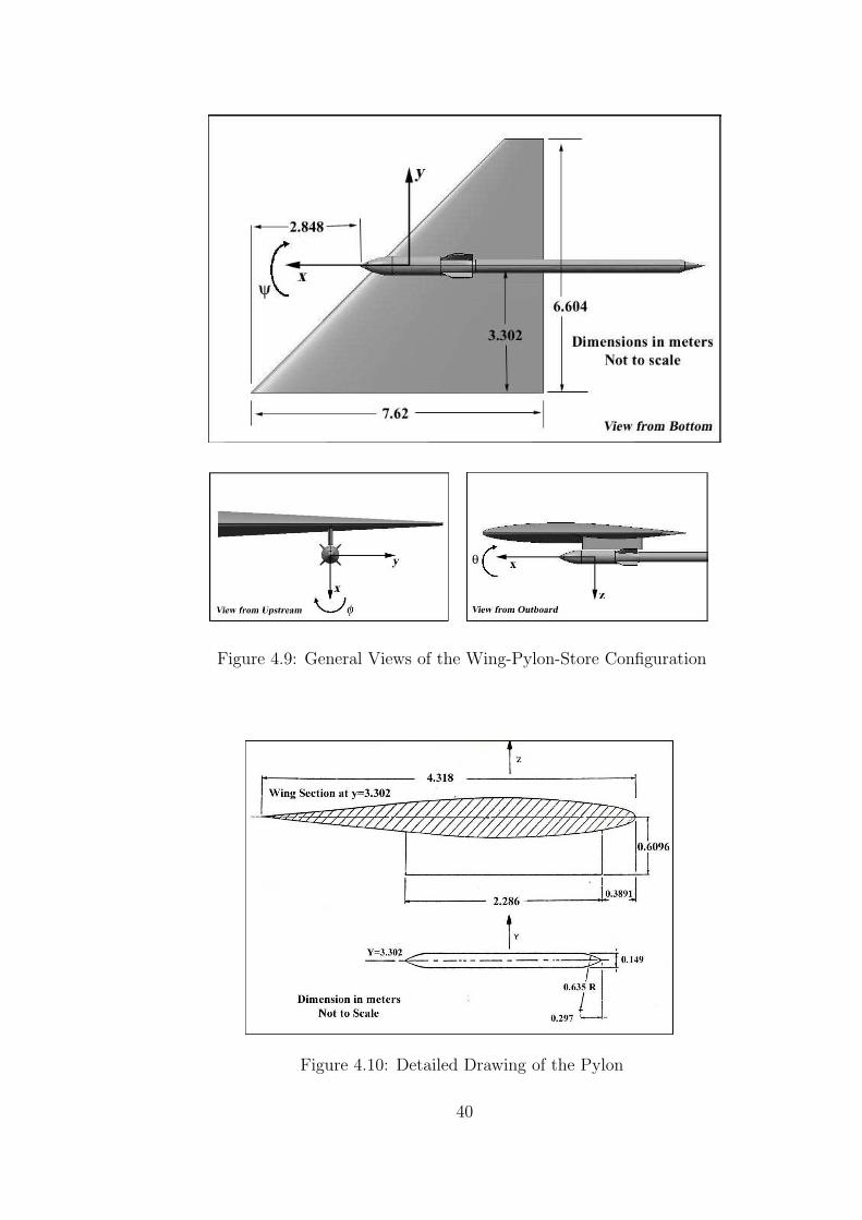
Figure 4.9: General Views of the Wing-Pylon-Store Configuration

Figure 4.10: Detailed Drawing of the Pylon

40

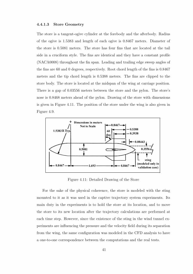
4.4.1.3 Store Geometry

The store is a tangent-ogive cylinder at the forebody and the afterbody. Radius

of the ogive is 1.5383 and length of each ogive is 0.8467 meters. Diameter of

the store is 0.5081 meters. The store has four fins that are located at the tail

side in a cruciform style. The fins are identical and they have a constant profile

(NACA0008) throughout the fin span. Leading and trailing edge sweep angles of

the fins are 60 and 0 degrees, respectively. Root chord length of the fins is 0.8467

meters and the tip chord length is 0.5388 meters. The fins are clipped to the

store body. The store is located at the midspan of the wing at carriage position.

There is a gap of 0.03556 meters between the store and the pylon. The store’s

nose is 0.8468 meters ahead of the pylon. Drawing of the store with dimensions

is given in Figure 4.11. The position of the store under the wing is also given in

Figure 4.9.

Figure 4.11: Detailed Drawing of the Store

For the sake of the physical coherence, the store is modeled with the sting

mounted to it as it was used in the captive trajectory system experiments. Its

main duty in the experiments is to hold the store at its location, and to move

the store to its new location after the trajectory calculations are performed at

each time step. However, since the existence of the sting in the wind tunnel ex-

periments are influencing the pressure and the velocity field during its separation

from the wing, the same configuration was modeled in the CFD analysis to have

a one-to-one correspondence between the computations and the real tests.

41

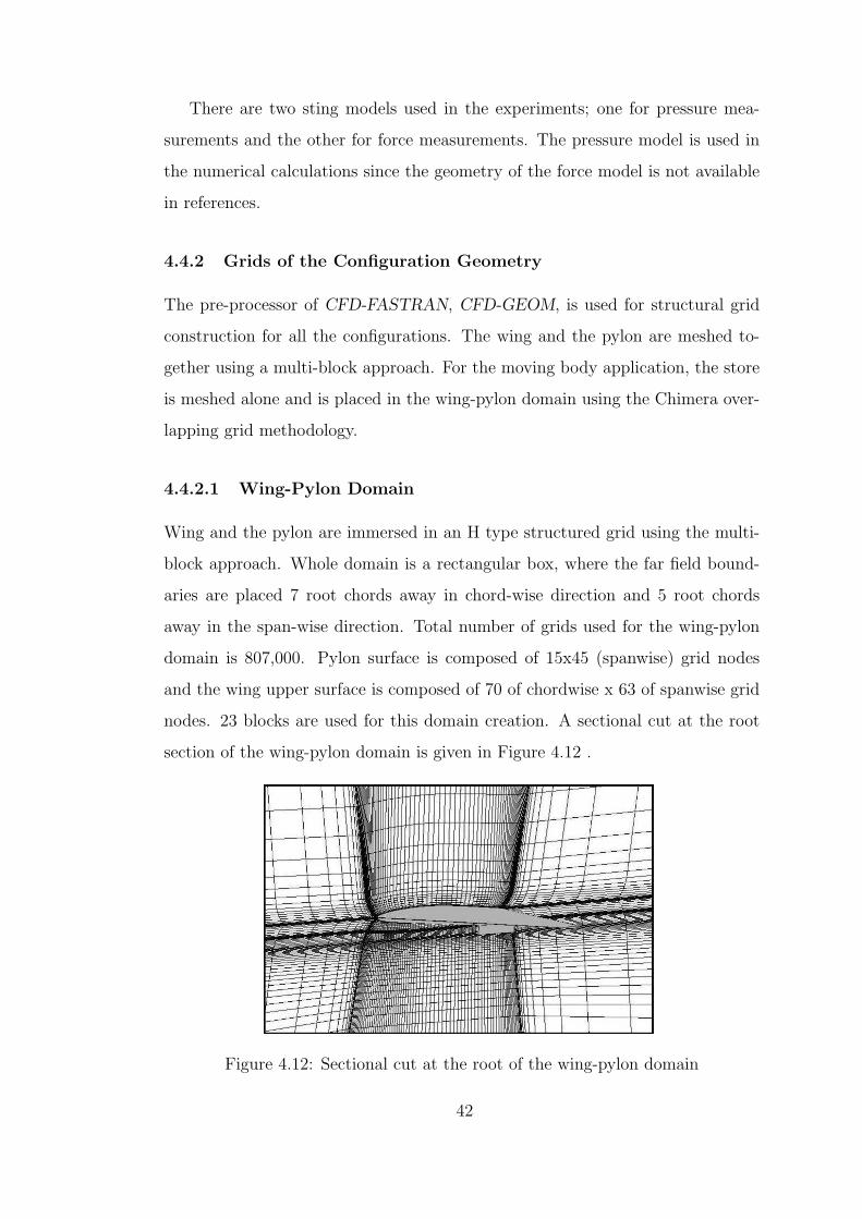
There are two sting models used in the experiments; one for pressure mea-

surements and the other for force measurements. The pressure model is used in

the numerical calculations since the geometry of the force model is not available

in references.

4.4.2 Grids of the Configuration Geometry

The pre-processor of CFD-FASTRAN, CFD-GEOM, is used for structural grid

construction for all the configurations. The wing and the pylon are meshed to-

gether using a multi-block approach. For the moving body application, the store

is meshed alone and is placed in the wing-pylon domain using the Chimera over-

lapping grid methodology.

4.4.2.1 Wing-Pylon Domain

Wing and the pylon are immersed in an H type structured grid using the multi-

block approach. Whole domain is a rectangular box, where the far field bound-

aries are placed 7 root chords away in chord-wise direction and 5 root chords

away in the span-wise direction. Total number of grids used for the wing-pylon

domain is 807,000. Pylon surface is composed of 15x45 (spanwise) grid nodes

and the wing upper surface is composed of 70 of chordwise x 63 of spanwise grid

nodes. 23 blocks are used for this domain creation. A sectional cut at the root

section of the wing-pylon domain is given in Figure 4.12 .

Figure 4.12: Sectional cut at the root of the wing-pylon domain

42

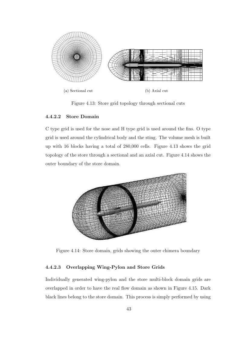
(a) Sectional cut (b) Axial cut

Figure 4.13: Store grid topology through sectional cuts

4.4.2.2 Store Domain

C type grid is used for the nose and H type grid is used around the fins. O type

grid is used around the cylindrical body and the sting. The volume mesh is built

up with 16 blocks having a total of 280,000 cells. Figure 4.13 shows the grid

topology of the store through a sectional and an axial cut. Figure 4.14 shows the

outer boundary of the store domain.

Figure 4.14: Store domain, grids showing the outer chimera boundary

4.4.2.3 Overlapping Wing-Pylon and Store Grids

Individually generated wing-pylon and the store multi-block domain grids are

overlapped in order to have the real flow domain as shown in Figure 4.15. Dark

black lines belong to the store domain. This process is simply performed by using

43

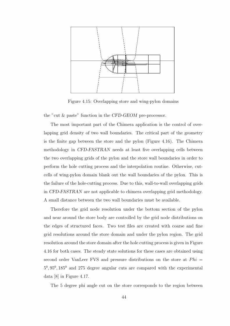
Figure 4.15: Overlapping store and wing-pylon domains

the ”cut & paste” function in the CFD-GEOM pre-processor.

The most important part of the Chimera application is the control of over-

lapping grid density of two wall boundaries. The critical part of the geometry

is the finite gap between the store and the pylon (Figure 4.16). The Chimera

methodology in CFD-FASTRAN needs at least five overlapping cells between

the two overlapping grids of the pylon and the store wall boundaries in order to

perform the hole cutting process and the interpolation routine. Otherwise, cut-

cells of wing-pylon domain blank out the wall boundaries of the pylon. This is

the failure of the hole-cutting process. Due to this, wall-to-wall overlapping grids

in CFD-FASTRAN are not applicable to chimera overlapping grid methodology.

A small distance between the two wall boundaries must be available.

Therefore the grid node resolution under the bottom section of the pylon

and near around the store body are controlled by the grid node distributions on

the edges of structured faces. Two test files are created with coarse and fine

grid resolutions around the store domain and under the pylon region. The grid

resolution around the store domain after the hole cutting process is given in Figure

4.16 for both cases. The steady state solutions for these cases are obtained using

second order VanLeer FVS and pressure distributions on the store at Phi =

50, 950, 1850 and 275 degree angular cuts are compared with the experimental

data [8] in Figure 4.17.

The 5 degree phi angle cut on the store corresponds to the region between

44

(a) Coarse Mesh (b) Fine Mesh

Figure 4.16: Grid around the store, between the store and the pylon

the pylon and the store where there is a significant interaction between two wall

boundaries. Both coarse and fine meshes around the store and under the pylon

solutions captures the compression due to pylon at X/L = 0.25. However, the

expansion after this compression is only captured perfectly with the finer mesh

distribution.

There are some discrepancies between the fine grid solutions and the available

data due to inviscid nature of the solver. However, for all angular section cuts,

the results are in better agreement with the data than the coarse mesh solutions.

The grid node distribution along the separation trajectory of the store under

the wing is finer than the upper side of the wing. This is a guarantee for finding the

donor cell for the chimera boundary cells of store domain and the wing domain.

4.4.3 Solution Parameters

This section describes the parameters which are used in the solution of the vali-

dation test case. These parameters are explained under the sections of initial and

boundary conditions, solver settings, convergence criteria, chimera methodology,

transient solution and moving body parameters in detail.

4.4.3.1 Initial and Boundary Conditions

All domains are initialized with the freestream values in steady solutions. These

freestream velocity, pressure and temperature values are given in Table 4.2. These

45

+

+

+

+

++

++ + +

+ ++

++ + + + +

+

+ ++

+

+

+

++

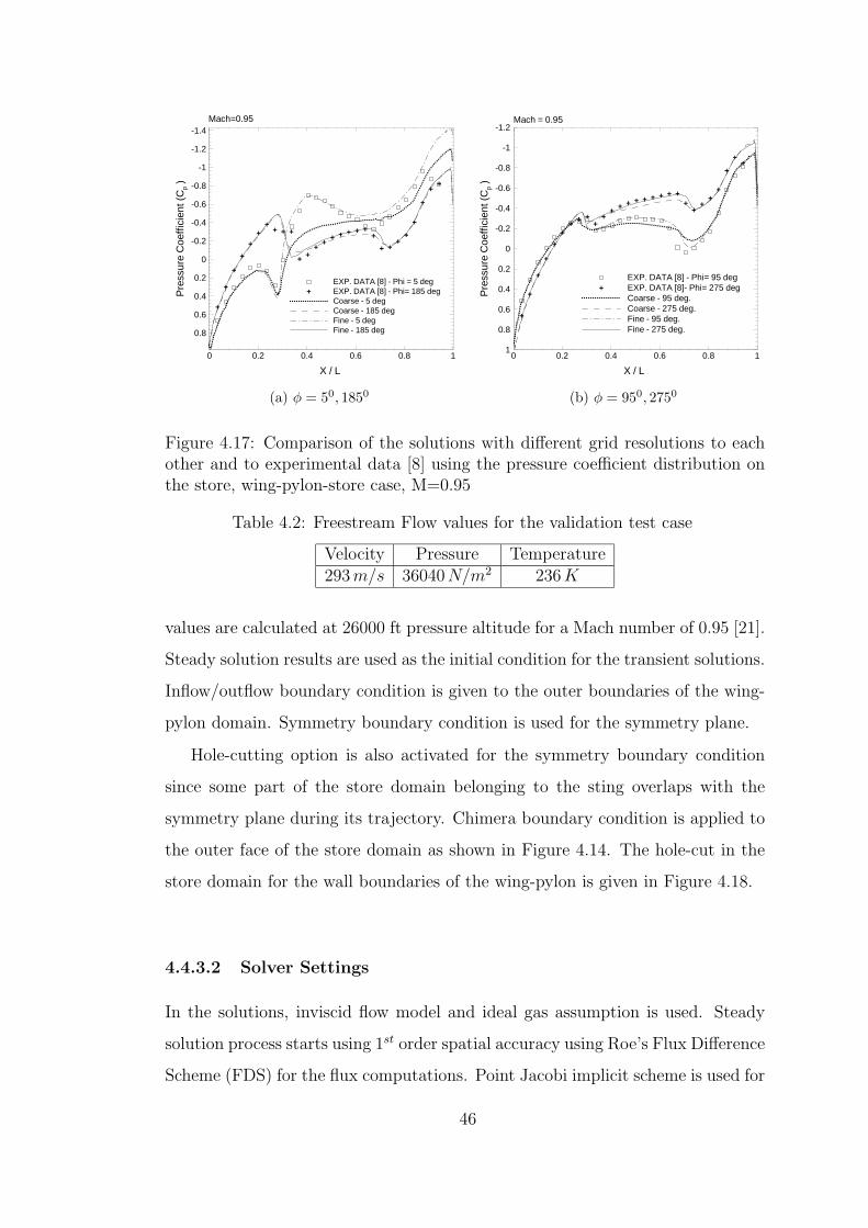
X / L

Pre

ssur

eC

oeff

icie

nt(C

p)

0 0.2 0.4 0.6 0.8 1

-1.4

-1.2

-1

-0.8

-0.6

-0.4

-0.2

0

0.2

0.4

0.6

0.8

EXP. DATA [8] - Phi = 5 degEXP. DATA [8] - Phi= 185 degCoarse - 5 degCoarse - 185 degFine - 5 degFine - 185 deg

+

Mach=0.95

(a) φ = 50, 1850

+

+

+

+

+

++ + +

++

+ + + + + + + + ++

++

++

+

++

X / L

Pre

ssur

eC

oeff

icie

nt(C

p)

0 0.2 0.4 0.6 0.8 1

-1.2

-1

-0.8

-0.6

-0.4

-0.2

0

0.2

0.4

0.6

0.8

1

EXP. DATA [8] - Phi= 95 degEXP. DATA [8]- Phi= 275 degCoarse - 95 deg.Coarse - 275 deg.Fine - 95 deg.Fine - 275 deg.

+

Mach = 0.95

(b) φ = 950, 2750

Figure 4.17: Comparison of the solutions with different grid resolutions to eachother and to experimental data [8] using the pressure coefficient distribution onthe store, wing-pylon-store case, M=0.95

Table 4.2: Freestream Flow values for the validation test case

Velocity Pressure Temperature293 m/s 36040N/m2 236 K

values are calculated at 26000 ft pressure altitude for a Mach number of 0.95 [21].

Steady solution results are used as the initial condition for the transient solutions.

Inflow/outflow boundary condition is given to the outer boundaries of the wing-

pylon domain. Symmetry boundary condition is used for the symmetry plane.

Hole-cutting option is also activated for the symmetry boundary condition

since some part of the store domain belonging to the sting overlaps with the

symmetry plane during its trajectory. Chimera boundary condition is applied to

the outer face of the store domain as shown in Figure 4.14. The hole-cut in the

store domain for the wall boundaries of the wing-pylon is given in Figure 4.18.

4.4.3.2 Solver Settings

In the solutions, inviscid flow model and ideal gas assumption is used. Steady

solution process starts using 1st order spatial accuracy using Roe’s Flux Difference

Scheme (FDS) for the flux computations. Point Jacobi implicit scheme is used for

46

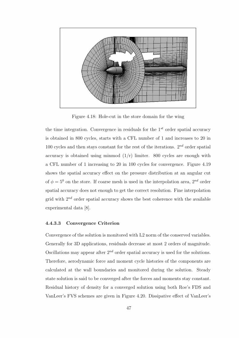
Figure 4.18: Hole-cut in the store domain for the wing

the time integration. Convergence in residuals for the 1st order spatial accuracy

is obtained in 800 cycles, starts with a CFL number of 1 and increases to 20 in

100 cycles and then stays constant for the rest of the iterations. 2nd order spatial

accuracy is obtained using minmod (1/r) limiter. 800 cycles are enough with

a CFL number of 1 increasing to 20 in 100 cycles for convergence. Figure 4.19

shows the spatial accuracy effect on the pressure distribution at an angular cut

of φ = 50 on the store. If coarse mesh is used in the interpolation area, 2nd order

spatial accuracy does not enough to get the correct resolution. Fine interpolation

grid with 2nd order spatial accuracy shows the best coherence with the available

experimental data [8].

4.4.3.3 Convergence Criterion

Convergence of the solution is monitored with L2 norm of the conserved variables.

Generally for 3D applications, residuals decrease at most 2 orders of magnitude.

Oscillations may appear after 2nd order spatial accuracy is used for the solutions.

Therefore, aerodynamic force and moment cycle histories of the components are

calculated at the wall boundaries and monitored during the solution. Steady

state solution is said to be converged after the forces and moments stay constant.

Residual history of density for a converged solution using both Roe’s FDS and

VanLeer’s FVS schemes are given in Figure 4.20. Dissipative effect of VanLeer’s

47

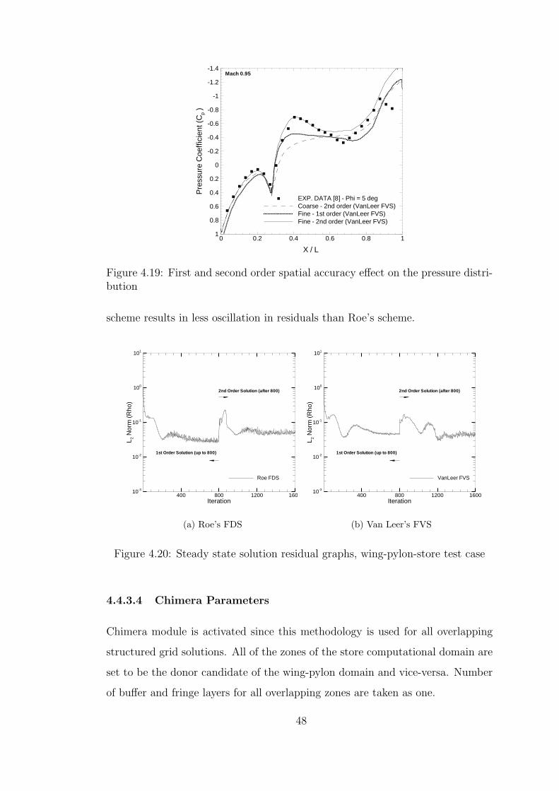
X / L

Pre

ssur

eC

oeff

icie

nt(C

p)

0 0.2 0.4 0.6 0.8 1

-1.4

-1.2

-1

-0.8

-0.6

-0.4

-0.2

0

0.2

0.4

0.6

0.8

1

EXP. DATA [8] - Phi = 5 degCoarse - 2nd order (VanLeer FVS)Fine - 1st order (VanLeer FVS)Fine - 2nd order (VanLeer FVS)

Mach 0.95

Figure 4.19: First and second order spatial accuracy effect on the pressure distri-bution

scheme results in less oscillation in residuals than Roe’s scheme.

Iteration

L 2N

orm

(Rho

)

400 800 1200 160010-3

10-2

10-1

100

101

Roe FDS

2nd Order Solution (after 800)

1st Order Solution (up to 800)

(a) Roe’s FDS

Iteration

L 2N

orm

(Rho

)

400 800 1200 160010-3

10-2

10-1

100

101

VanLeer FVS

2nd Order Solution (after 800)

1st Order Solution (up to 800)

(b) Van Leer’s FVS

Figure 4.20: Steady state solution residual graphs, wing-pylon-store test case

4.4.3.4 Chimera Parameters

Chimera module is activated since this methodology is used for all overlapping

structured grid solutions. All of the zones of the store computational domain are

set to be the donor candidate of the wing-pylon domain and vice-versa. Number

of buffer and fringe layers for all overlapping zones are taken as one.

48

NON-MOVING Grids

(Wing+pylon)

MOVING Chimera Grid

(Store)

Comp. Domain (wing+pylon+store)

Initial Conditions

+ = Steady-state

solution

t o =0

t=t o +dt

Unsteady solution

6DOF module

Forces on

moving body

Displacements

Rotations

Move chimera grid to its new

location

Target

POST PROCESS

YES

t=t o +n.dt

NO

Figure 4.21: Main steps taken in the solution of the store separation problem

4.4.3.5 Transient Solution and Moving Body Parameters

Transient solutions are used for the trajectory calculations of the store after its

separation from the wing. Figure 4.21 shows the placement of the transient

solutions in the store separation problem.

Time step is calculated for each cell by the solver using the CFL number given

as input parameter. The smallest time step is chosen and used as the global time

step for the unsteady solutions. The corresponding time step for the given CFL

number can be found from the output data. For the present calculations, a time

step of 0.00005 is used as the ∆t value. This time step is obtained using a CFL

number of 7140.

Steady state solutions are assigned as the initial condition for the transient

solutions. Since the local time stepping is used for the steady calculations, there

is a passage of CFL number of 20 to a higher value of 7140, which is used .

This transition is accomplished by carrying on the solutions using a global time

stepping method after the steady solutions are converged. During these transient

calculations, CFL number is increased from 20 to 7140 in 1000 cycles.

Moving Body module is activated using the GUI. Using motion models setup

menu, necessary input parameters are given to the solver. First, body coordinate

49

Table 4.3: Solution parameters used in the Wing-Pylon-Store validation case[21]

Weight of the store 2000lbCenter of gravity 4.65ft aft of store noseAft ejector location 5.73ft aft of store noseAft ejector force 9600lbForward ejector location 4.06ft aft of store noseForward ejector force 2400lbEjector store length 0.33ftRoll moment of inertia,Ixx 20slug − ft2Pitch moment of inertia,Iyy 360slug − ft2Yaw moment of inertia, Izz 360slug − ft2Freestream Mach number 0.95Aircraft angle of attack 0.0deg.Pressure Altitude 26000ft

system for the store is defined. The c.g. location of the store is chosen for the

origin of this axis system. Mass and moment of inertia values for the store is given

next. The forces acting on the store which are used for the trajectory calcula-

tions are selected in the same menu. For the present calculations, aerodynamic,

gravitational and point forces are taken into account.

Aerodynamic force input requires the zone numbers of the store domain. The

zones of the sting are not used in the aerodynamic force calculations. Therefore,

multi-block grid generation is required for moving body problems if any section

of the body is not used for the aerodynamic force calculations.

Point forces are used for the ejector force modelling. Any number of point

forces can be added to the simulation. Frame of reference is chosen as the inertial

axis for the ejector force applications. Point of application of the ejector force

is defined in the inertial coordinate axis system. Ejector force applied can be a

function of time or any of the three axis and three rotations. In this study, ejector

forces are taken as constant and applied on the store until the store displaces 0.1

meters in downward direction in the inertial axis coordinate system.

Finally, using the Set-up Grid Motions menu, the zones that will move with

the body coordinate axis system is chosen. The zones of the store and the sting

are chosen together at this time. The parameters related to the validation test

case are summarized and given in Table 4.3.

50

+ + + + + + + + + + + + + + + + + + + + + + + + + + + + + + + + + + + + + ++ + +

+ ++

++

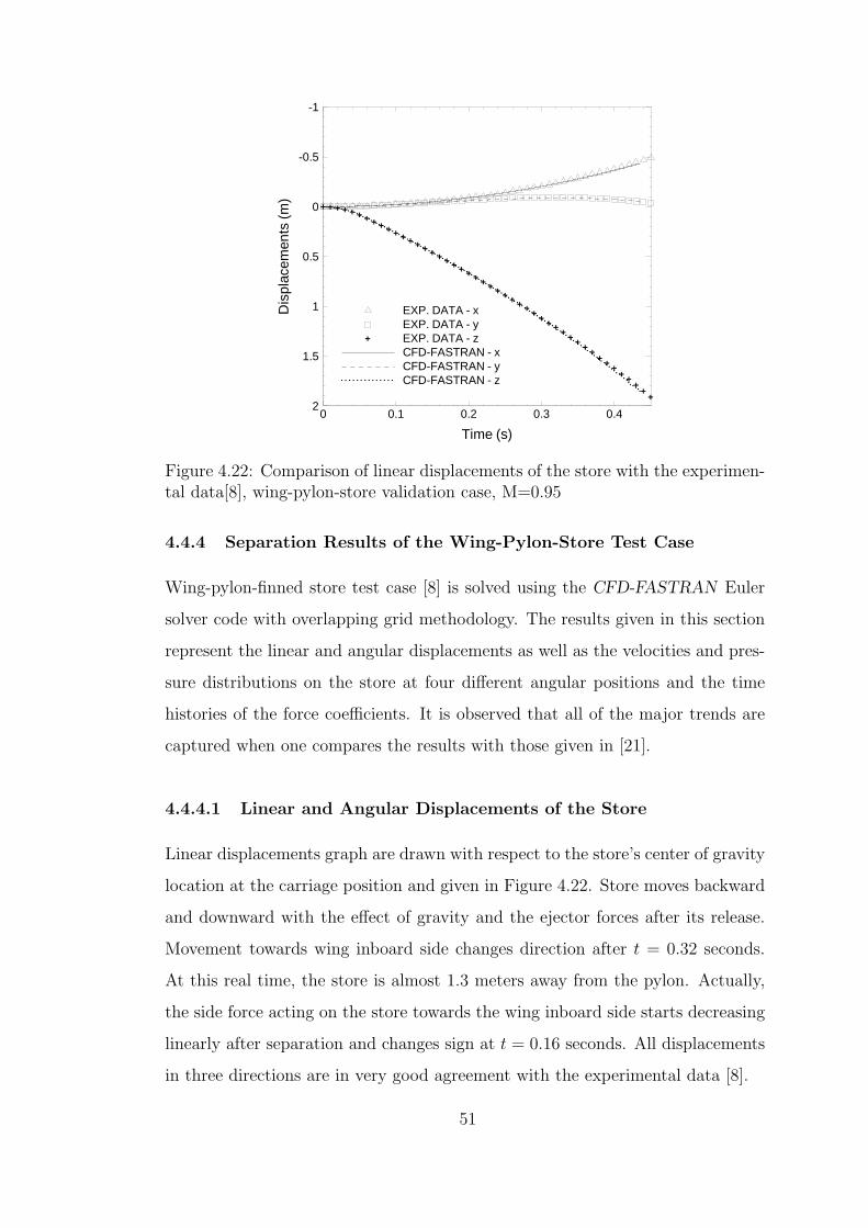
Time (s)

Dis

plac

emen

ts(m

)

0 0.1 0.2 0.3 0.4

-1

-0.5

0

0.5

1

1.5

2

EXP. DATA - xEXP. DATA - yEXP. DATA - zCFD-FASTRAN - xCFD-FASTRAN - yCFD-FASTRAN - z

+

Figure 4.22: Comparison of linear displacements of the store with the experimen-tal data[8], wing-pylon-store validation case, M=0.95

4.4.4 Separation Results of the Wing-Pylon-Store Test Case

Wing-pylon-finned store test case [8] is solved using the CFD-FASTRAN Euler

solver code with overlapping grid methodology. The results given in this section

represent the linear and angular displacements as well as the velocities and pres-

sure distributions on the store at four different angular positions and the time

histories of the force coefficients. It is observed that all of the major trends are

captured when one compares the results with those given in [21].

4.4.4.1 Linear and Angular Displacements of the Store

Linear displacements graph are drawn with respect to the store’s center of gravity

location at the carriage position and given in Figure 4.22. Store moves backward

and downward with the effect of gravity and the ejector forces after its release.

Movement towards wing inboard side changes direction after t = 0.32 seconds.

At this real time, the store is almost 1.3 meters away from the pylon. Actually,

the side force acting on the store towards the wing inboard side starts decreasing

linearly after separation and changes sign at t = 0.16 seconds. All displacements

in three directions are in very good agreement with the experimental data [8].

51

+ + + + + + + + + + + + + + + + + + + + + + + + + + + + + + + + + + + ++

++

++

++

++

+

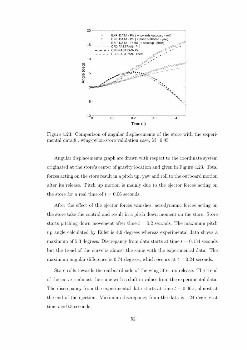
Time (s)

Ang

le(d

eg)

0 0.1 0.2 0.3 0.4-10

-5

0

5

10

15

20

EXP. DATA - Phi ( + towards outboard - roll)EXP. DATA - Psi ( + nose outboard - yaw)EXP. DATA - Theta ( + nose up - pitch)CFD-FASTRAN- PhiCFD-FASTRAN- PsiCFD-FASTRAN- Theta

+

Figure 4.23: Comparison of angular displacements of the store with the experi-mental data[8], wing-pylon-store validation case, M=0.95

Angular displacements graph are drawn with respect to the coordinate system

originated at the store’s center of gravity location and given in Figure 4.23. Total

forces acting on the store result in a pitch up, yaw and roll to the outboard motion

after its release. Pitch up motion is mainly due to the ejector forces acting on

the store for a real time of t = 0.06 seconds.

After the effect of the ejector forces vanishes, aerodynamic forces acting on

the store take the control and result in a pitch down moment on the store. Store

starts pitching down movement after time t = 0.2 seconds. The maximum pitch

up angle calculated by Euler is 4.9 degrees whereas experimental data shows a

maximum of 5.3 degrees. Discrepancy from data starts at time t = 0.134 seconds

but the trend of the curve is almost the same with the experimental data. The

maximum angular difference is 0.74 degrees, which occurs at t = 0.24 seconds.

Store rolls towards the outboard side of the wing after its release. The trend

of the curve is almost the same with a shift in values from the experimental data.

The discrepancy from the experimental data starts at time t = 0.06 s, almost at

the end of the ejection. Maximum discrepancy from the data is 1.24 degrees at

time t = 0.3 seconds.

52

+

+

+

+

+

++ + ++ +++ +++ + + + ++ + + + + ++ + ++ + ++ + + +

Time (s)

Vel

ocity

(m/s

)

0 0.1 0.2 0.3 0.4-3

-2

-1

0

1

2

3

4

5

6

7EXP. DATA - uEXP. DATA - vEXP. DATA - wCFD-FASTRAN - uCFD-FASTRAN - vCFD-FASTRAN - w

+

Figure 4.24: Comparison of linear velocities of the store with the experimentaldata[21], wing-pylon-store validation case, M=0.95

Yawing moment acting on the store is towards to the outboard of the wing.

The trend of the curve is again the same with the experimental data. The dis-

crepancy from the data starts at t = 0.17 seconds, and the difference increases

till the end of the calculations. The maximum difference between the present

calculations and the available data is 1.34 degrees.

4.4.4.2 Linear and Angular Velocities of the Store

Linear velocities of the store along its trajectory are given in Figure 4.24. Store

moves down with an almost constant acceleration of 62.21 m/s2 under the effect

of ejector forces and its weight until t = 0.06 s. After ejector forces disappear,

linear velocity in downward direction increases with a lower acceleration. There

is maximum discrepancy of 0.307 m/s between the data and the calculations.

Side velocity does not show a good agreement with the experimental data.

In the experimental data, store has a negative side velocity of v after its release

until time t = 0.2 seconds. However, present calculations have a time lag of 0.12

seconds for the side velocity to change its sign from negative to positive. At time

t = 0.32 seconds, the difference between the side velocity calculations and the

experimental data becomes 1.04 m/s.

53

+

+

+

+

+

+ ++

++

++

++

++

++

++

++

++

++

++

++

++

++

+ + + + + + + + + + + +

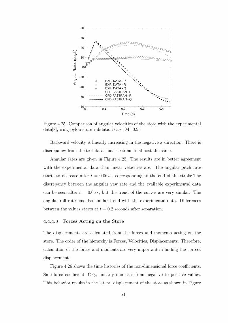
Time (s)

Ang

ular

Rat

es(d

eg/s

)

0 0.1 0.2 0.3 0.4-80

-60

-40

-20

0

20

40

60

80

EXP. DATA - PEXP. DATA - REXP. DATA - QCFD-FASTRAN - PCFD-FASTRAN - RCFD-FASTRAN - Q

+

Figure 4.25: Comparison of angular velocities of the store with the experimentaldata[8], wing-pylon-store validation case, M=0.95

Backward velocity is linearly increasing in the negative x direction. There is

discrepancy from the test data, but the trend is almost the same.

Angular rates are given in Figure 4.25. The results are in better agreement

with the experimental data than linear velocities are. The angular pitch rate

starts to decrease after t = 0.06 s , corresponding to the end of the stroke.The

discrepancy between the angular yaw rate and the available experimental data

can be seen after t = 0.06 s, but the trend of the curves are very similar. The

angular roll rate has also similar trend with the experimental data. Differences

between the values starts at t = 0.2 seconds after separation.

4.4.4.3 Forces Acting on the Store

The displacements are calculated from the forces and moments acting on the

store. The order of the hierarchy is Forces, Velocities, Displacements. Therefore,

calculation of the forces and moments are very important in finding the correct

displacements.

Figure 4.26 shows the time histories of the non-dimensional force coefficients.

Side force coefficient, CFy, linearly increases from negative to positive values.

This behavior results in the lateral displacement of the store as shown in Figure

54

+ + + + + + + + + + + + + + + + + + + + + + + + + + + + + + + ++

++

++

++

++

++

++

+

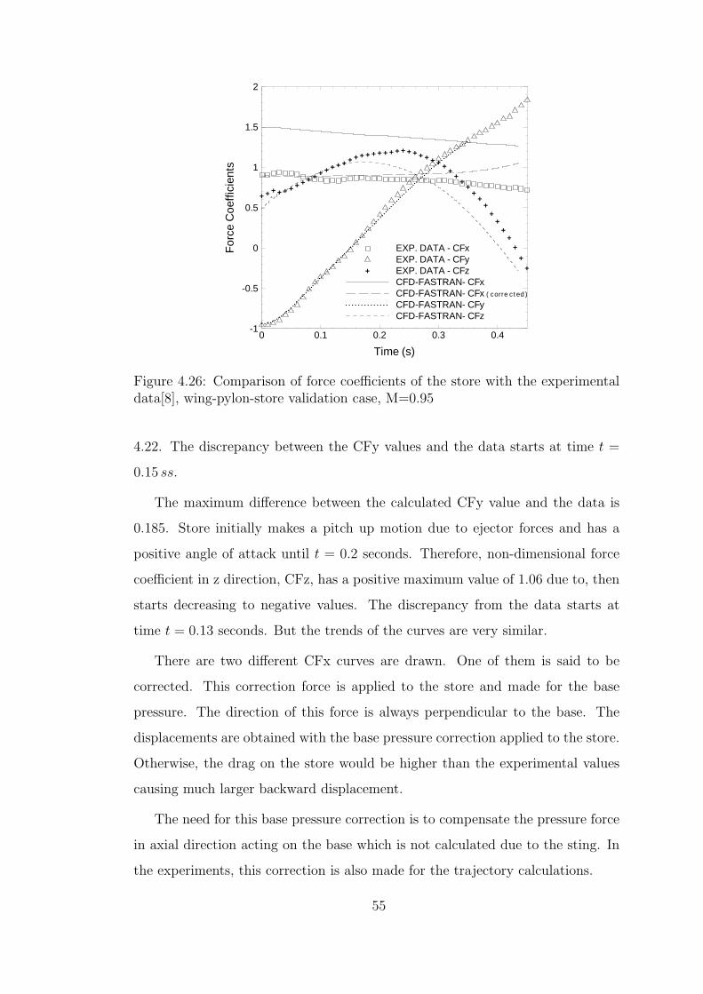
Time (s)

For

ceC

oeff

icie

nts

0 0.1 0.2 0.3 0.4-1

-0.5

0

0.5

1

1.5

2

EXP. DATA - CFxEXP. DATA - CFyEXP. DATA - CFzCFD-FASTRAN- CFxCFD-FASTRAN- CFx ( corre ct ed )

CFD-FASTRAN- CFyCFD-FASTRAN- CFz

+

Figure 4.26: Comparison of force coefficients of the store with the experimentaldata[8], wing-pylon-store validation case, M=0.95

4.22. The discrepancy between the CFy values and the data starts at time t =

0.15 ss.

The maximum difference between the calculated CFy value and the data is

0.185. Store initially makes a pitch up motion due to ejector forces and has a

positive angle of attack until t = 0.2 seconds. Therefore, non-dimensional force

coefficient in z direction, CFz, has a positive maximum value of 1.06 due to, then

starts decreasing to negative values. The discrepancy from the data starts at

time t = 0.13 seconds. But the trends of the curves are very similar.

There are two different CFx curves are drawn. One of them is said to be

corrected. This correction force is applied to the store and made for the base

pressure. The direction of this force is always perpendicular to the base. The

displacements are obtained with the base pressure correction applied to the store.

Otherwise, the drag on the store would be higher than the experimental values

causing much larger backward displacement.

The need for this base pressure correction is to compensate the pressure force

in axial direction acting on the base which is not calculated due to the sting. In

the experiments, this correction is also made for the trajectory calculations.

55

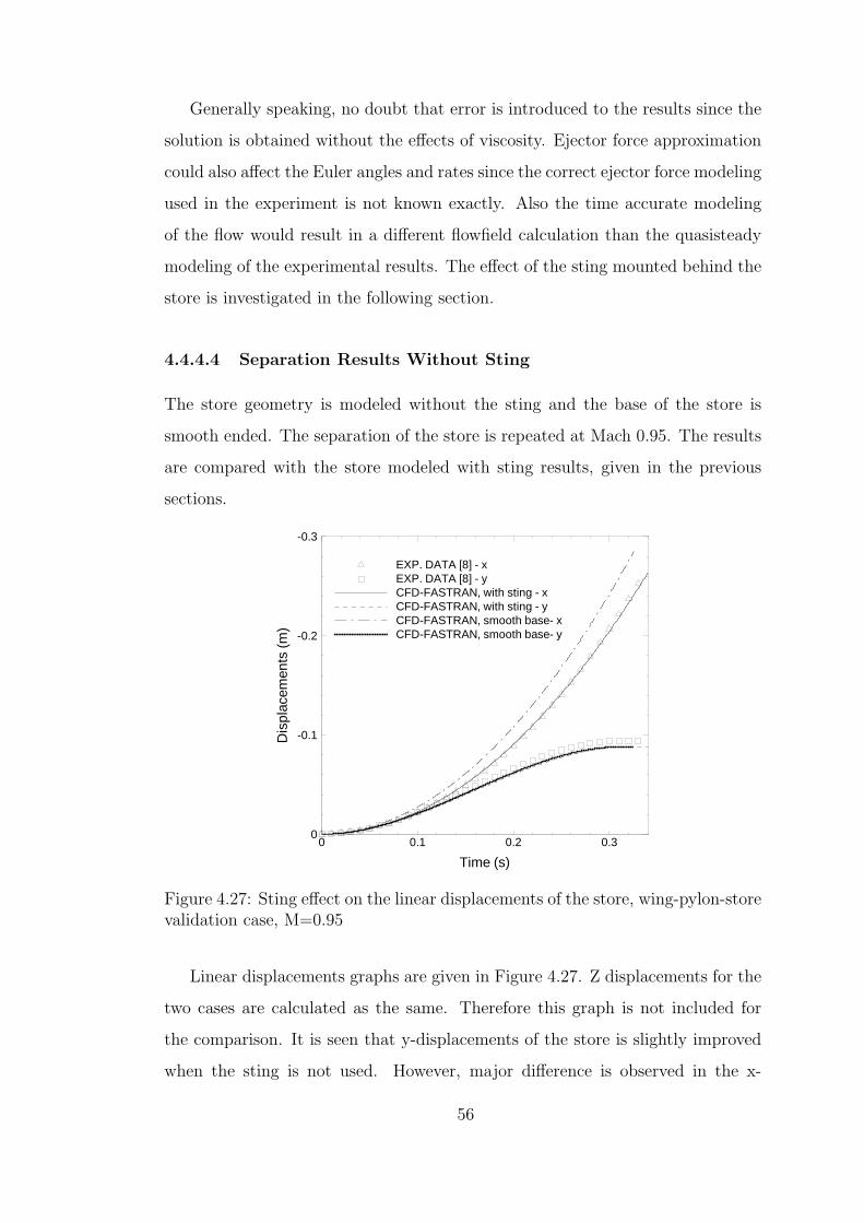
Generally speaking, no doubt that error is introduced to the results since the

solution is obtained without the effects of viscosity. Ejector force approximation

could also affect the Euler angles and rates since the correct ejector force modeling

used in the experiment is not known exactly. Also the time accurate modeling

of the flow would result in a different flowfield calculation than the quasisteady

modeling of the experimental results. The effect of the sting mounted behind the

store is investigated in the following section.

4.4.4.4 Separation Results Without Sting

The store geometry is modeled without the sting and the base of the store is

smooth ended. The separation of the store is repeated at Mach 0.95. The results

are compared with the store modeled with sting results, given in the previous

sections.

Time (s)

Dis

plac

emen

ts(m

)

0 0.1 0.2 0.3

-0.3

-0.2

-0.1

0

EXP. DATA [8] - xEXP. DATA [8] - yCFD-FASTRAN, with sting - xCFD-FASTRAN, with sting - yCFD-FASTRAN, smooth base- xCFD-FASTRAN, smooth base- y

Figure 4.27: Sting effect on the linear displacements of the store, wing-pylon-storevalidation case, M=0.95

Linear displacements graphs are given in Figure 4.27. Z displacements for the

two cases are calculated as the same. Therefore this graph is not included for

the comparison. It is seen that y-displacements of the store is slightly improved

when the sting is not used. However, major difference is observed in the x-

56

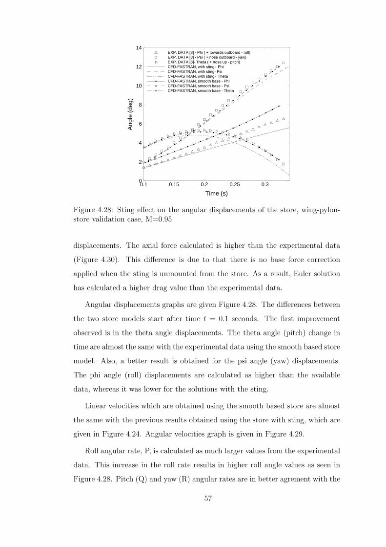
Time (s)

Ang

le(d

eg)

0.1 0.15 0.2 0.25 0.30

2

4

6

8

10

12

14EXP. DATA [8] - Phi ( + towards outboard - roll)EXP. DATA [8] - Psi ( + nose outboard - yaw)EXP. DATA [8]- Theta ( + nose up - pitch)CFD-FASTRAN, with sting- PhiCFD-FASTRAN, with sting- PsiCFD-FASTRAN, with sting- ThetaCFD-FASTRAN, smooth base - PhiCFD-FASTRAN, smooth base - PsiCFD-FASTRAN, smooth base - Theta

Figure 4.28: Sting effect on the angular displacements of the store, wing-pylon-store validation case, M=0.95

displacements. The axial force calculated is higher than the experimental data

(Figure 4.30). This difference is due to that there is no base force correction

applied when the sting is unmounted from the store. As a result, Euler solution

has calculated a higher drag value than the experimental data.

Angular displacements graphs are given Figure 4.28. The differences between

the two store models start after time t = 0.1 seconds. The first improvement

observed is in the theta angle displacements. The theta angle (pitch) change in

time are almost the same with the experimental data using the smooth based store

model. Also, a better result is obtained for the psi angle (yaw) displacements.

The phi angle (roll) displacements are calculated as higher than the available

data, whereas it was lower for the solutions with the sting.

Linear velocities which are obtained using the smooth based store are almost

the same with the previous results obtained using the store with sting, which are

given in Figure 4.24. Angular velocities graph is given in Figure 4.29.

Roll angular rate, P, is calculated as much larger values from the experimental

data. This increase in the roll rate results in higher roll angle values as seen in

Figure 4.28. Pitch (Q) and yaw (R) angular rates are in better agrement with the

57

+

+

+

+

+

+ ++

++

++

++

++

++

++

++

++

++

++

++

++

++

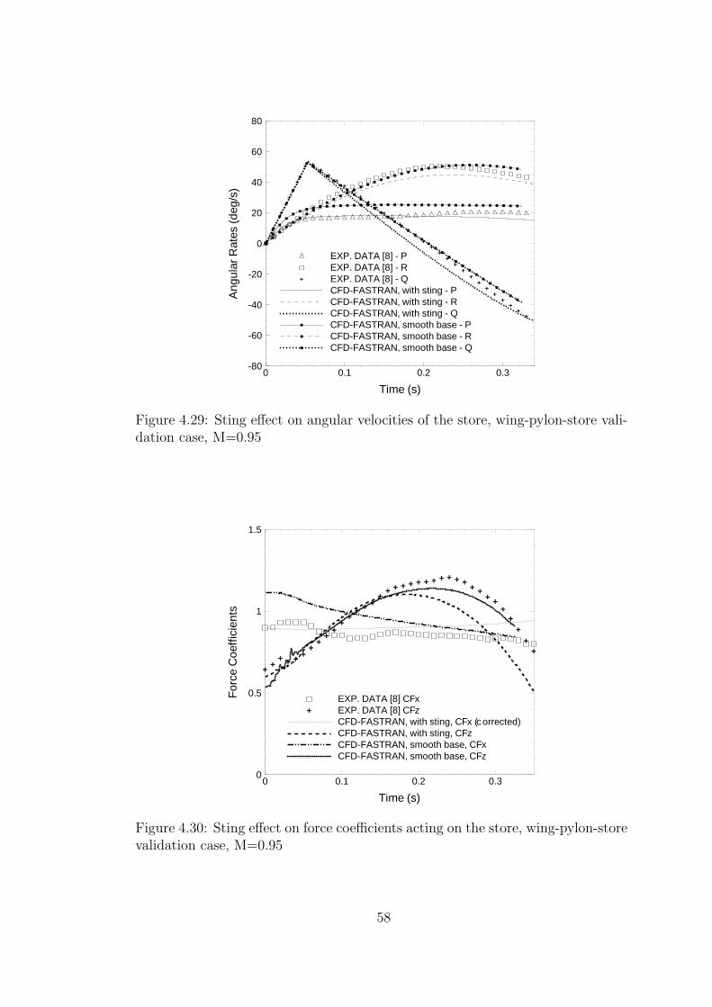
Time (s)

Ang

ular

Rat

es(d

eg/s

)

0 0.1 0.2 0.3-80

-60

-40

-20

0

20

40

60

80

EXP. DATA [8] - PEXP. DATA [8] - REXP. DATA [8] - QCFD-FASTRAN, with sting - PCFD-FASTRAN, with sting - RCFD-FASTRAN, with sting - QCFD-FASTRAN, smooth base - PCFD-FASTRAN, smooth base - RCFD-FASTRAN, smooth base - Q

+

Figure 4.29: Sting effect on angular velocities of the store, wing-pylon-store vali-dation case, M=0.95

++

+ + + ++

++

++

++ + +

++ + + + + + + + + + +

+ ++ +

++

++

+

Time (s)

For

ceC

oeff

icie

nts

0 0.1 0.2 0.30

0.5

1

1.5

EXP. DATA [8] CFxEXP. DATA [8] CFzCFD-FASTRAN, with sting, CFx (c orrected)CFD-FASTRAN, with sting, CFzCFD-FASTRAN, smooth base, CFxCFD-FASTRAN, smooth base, CFz

+

Figure 4.30: Sting effect on force coefficients acting on the store, wing-pylon-storevalidation case, M=0.95

58

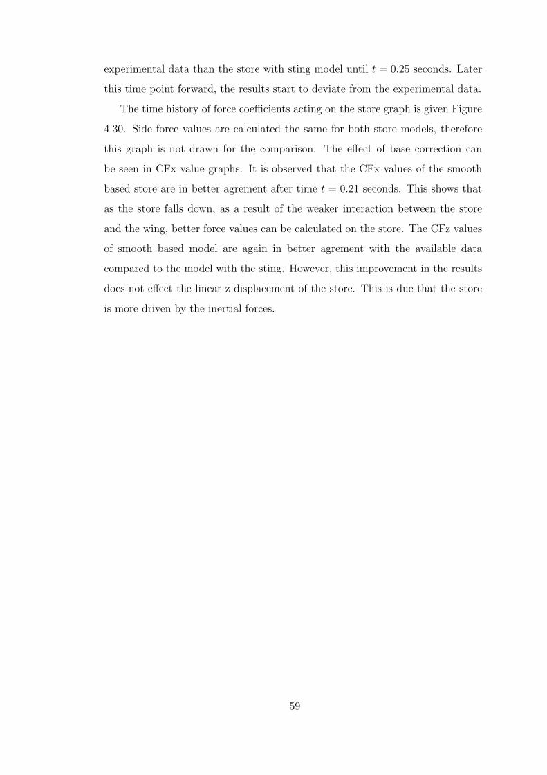
experimental data than the store with sting model until t = 0.25 seconds. Later

this time point forward, the results start to deviate from the experimental data.

The time history of force coefficients acting on the store graph is given Figure

4.30. Side force values are calculated the same for both store models, therefore

this graph is not drawn for the comparison. The effect of base correction can

be seen in CFx value graphs. It is observed that the CFx values of the smooth

based store are in better agrement after time t = 0.21 seconds. This shows that

as the store falls down, as a result of the weaker interaction between the store

and the wing, better force values can be calculated on the store. The CFz values

of smooth based model are again in better agrement with the available data

compared to the model with the sting. However, this improvement in the results

does not effect the linear z displacement of the store. This is due that the store

is more driven by the inertial forces.

59

CHAPTER 5

RESULTS AND DISCUSSION

5.1 Overview

This chapter presents the results of two different store separation cases studied.

The first case is the separation of a finned store from a wing-pylon configuration

at Mach numbers of 0.3 and 0.6. The second case is the separation of a fueltank

from an F-16 aircraft wing alone and the full aircraft configurations. The first case

is solved with both the Euler using the chimera methodology and the unsteady

panel codes. The second case is solved only using the unsteady panel code. The

aim is to compare the two methods of prediction tools and to find out which

aspects of the store separation phenomenon could be captured with these two

different prediction tools. The results are given in terms of time wise variations

of the linear and angular displacements of the store along its trajectory after being

released, the pressure distribution on the store in its captive position (t = 0 s)

right before its separation and the time histories of the force coefficients acting

on the store along its trajectory.

5.2 Configurations

Two different configurations are used in the present solutions. The first config-

uration is the generic wing-pylon-store configuration. The sting which was used

in the validation studies is not modeled this time. Instead, the base of the store

60

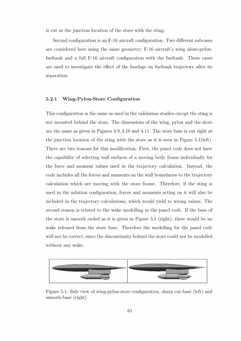
is cut at the junction location of the store with the sting.

Second configuration is an F-16 aircraft configuration. Two different subcases

are considered here using the same geometry; F-16 aircraft’s wing alone-pylon-

fueltank and a full F-16 aircraft configuration with the fueltank. These cases

are used to investigate the effect of the fuselage on fueltank trajectory after its

separation.

5.2.1 Wing-Pylon-Store Configuration

This configuration is the same as used in the validation studies except the sting is

not mounted behind the store. The dimensions of the wing, pylon and the store

are the same as given in Figures 4.9, 4.10 and 4.11. The store base is cut right at

the junction location of the sting with the store as it is seen in Figure 5.1(left).

There are two reasons for this modification. First, the panel code does not have

the capability of selecting wall surfaces of a moving body frame individually for

the force and moment values used in the trajectory calculation. Instead, the

code includes all the forces and moments on the wall boundaries to the trajectory

calculation which are moving with the store frame. Therefore, if the sting is

used in the solution configuration, forces and moments acting on it will also be

included in the trajectory calculations, which would yield to wrong values. The

second reason is related to the wake modelling in the panel code. If the base of

the store is smooth ended as it is given in Figure 5.1 (right), there would be no

wake released from the store base. Therefore the modelling for the panel code

will not be correct, since the discontinuity behind the store could not be modelled

without any wake.

Figure 5.1: Side view of wing-pylon-store configuration, sharp cut-base (left) andsmooth-base (right)

61

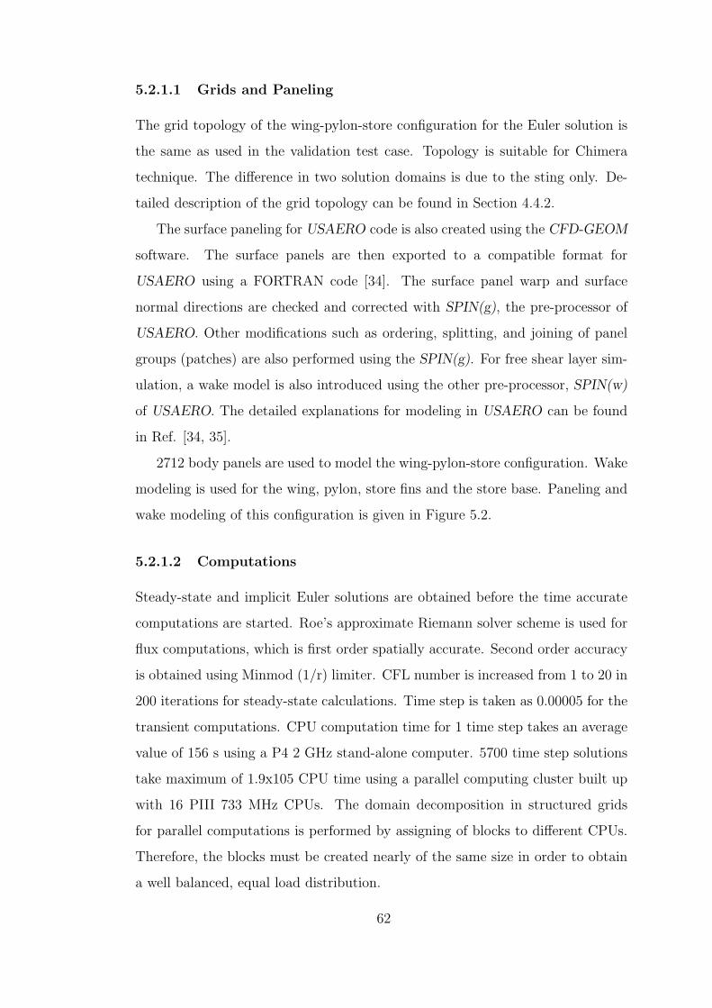
5.2.1.1 Grids and Paneling

The grid topology of the wing-pylon-store configuration for the Euler solution is

the same as used in the validation test case. Topology is suitable for Chimera

technique. The difference in two solution domains is due to the sting only. De-

tailed description of the grid topology can be found in Section 4.4.2.

The surface paneling for USAERO code is also created using the CFD-GEOM

software. The surface panels are then exported to a compatible format for

USAERO using a FORTRAN code [34]. The surface panel warp and surface

normal directions are checked and corrected with SPIN(g), the pre-processor of

USAERO. Other modifications such as ordering, splitting, and joining of panel

groups (patches) are also performed using the SPIN(g). For free shear layer sim-

ulation, a wake model is also introduced using the other pre-processor, SPIN(w)

of USAERO. The detailed explanations for modeling in USAERO can be found

in Ref. [34, 35].

2712 body panels are used to model the wing-pylon-store configuration. Wake

modeling is used for the wing, pylon, store fins and the store base. Paneling and

wake modeling of this configuration is given in Figure 5.2.

5.2.1.2 Computations

Steady-state and implicit Euler solutions are obtained before the time accurate

computations are started. Roe’s approximate Riemann solver scheme is used for

flux computations, which is first order spatially accurate. Second order accuracy

is obtained using Minmod (1/r) limiter. CFL number is increased from 1 to 20 in

200 iterations for steady-state calculations. Time step is taken as 0.00005 for the

transient computations. CPU computation time for 1 time step takes an average

value of 156 s using a P4 2 GHz stand-alone computer. 5700 time step solutions

take maximum of 1.9x105 CPU time using a parallel computing cluster built up

with 16 PIII 733 MHz CPUs. The domain decomposition in structured grids

for parallel computations is performed by assigning of blocks to different CPUs.

Therefore, the blocks must be created nearly of the same size in order to obtain

a well balanced, equal load distribution.

62

Figure 5.2: Paneling and wake modeling of wing-pylon-store configuration forUSAERO

For the unsteady panel code solutions a time step of 0.001 is used. 30 time

steps are used in order to establish the wake before the separation process starts.

Boundary layers are taken into account by activating the integral boundary layer

method coupling with potential flow solution. A direct matrix solver, LAPACK,

is used for the matrix inversions. Solutions are obtained using a SGI-Octane

stand-alone computer. The average CPU time needed for a time step of solution

using 2712 surface panels including wake panels is around 106 seconds. The first

time step takes a CPU time (without wakes) of 22.67 seconds and the last time

step takes 208.80 seconds. F-16 aircraft configuration with 6046 body panels takes

about 20 hours of CPU time for 0.32 seconds of real time duration of transient

solution.

5.2.1.3 Smooth base-Sharp Cut base Force Comparisons

In Euler solution, calculated drag values include the pressure forces, but excludes

the viscous effects. Due to inviscid nature of the flow, base drag value could not

be calculated correctly. The panel code gives drag value after the boundary layer

coupling, therefore the total drag predicted by the panel/boundary layer method

includes the skin friction drag as well.

Base wake model is used in USAERO for the flow separation at the base-cut

section. In order to investigate the effect of base cut and the separated flow,

63

a series of test cases are run with both codes using the configurations given in

Figure 5.1. Mach number is taken as 0.3. The store base is smoothed in order

to have a reasonably attached base flow. Base wake model is not used for this

case in USAERO solution. The comparison of the resultant force and moment

coefficients with the base-cut model are given in Tables 5.1 and 5.2, respectively.

The drag values which are calculated for smooth base configurations are very

close to each other. It is observed that smoothing the base of the store reduces

the drag value as obtained by the Euler code. The reverse effect is observed

when the panel code is used. Drag value is reduced when the base wake model

is introduced to the solution. The normal force coefficient CFz is found to be

the same using both methods for the base-cut configuration. Side force value is

found to be half of the panel code when the Euler code is used.

Table 5.1: Force coefficients on the store in its captive position, smooth andsharp-cut base comparisons, M=0.3

Smooth base CFx CFy CFz Sharp cut base CFx CFy CFz

FASTRAN 0.214 -0.444 0.511 FASTRAN 0.384 -0.449 0.695USAERO 0.196 -0.227 0.668 USAERO 0.128 -0.285 0.695

Table 5.2: Moment coefficients on the store wrt. c.g. location in its captiveposition, smooth and sharp-cut base comparisons, M=0.3

Smooth base CMx CMy CMz Sharp cut base CMx CMy CMz

FASTRAN 0.0945 1.2307 0.1153 FASTRAN 0.0967 1.702 0.1261USAERO 0.0101 1.3082 0.2099 USAERO 0.0110 1.465 0.0225

5.2.2 F-16 Aircraft Configurations

F-16 Fighting Falcon is a multi-role fighter aircraft in TUAF. This aircraft was

previously analyzed by [35, 36] using CFD tools. In Ref [35], aerodynamic analysis

of external store carriage on the same aircraft was investigated using the panel

code, VSAERO. It is a low order panel code, which is the steady version of the

unsteady panel code USAERO. In the other Ref [36], loads on different stores are

calculated at the carriage position using the same Euler code CFD-FASTRAN.

In this study, solutions were obtained using the unstructured grids. Both of these

previous studies were concentrated on the effect of the stores on the aircraft

64

Figure 5.3: F-16 Wing-Pylon-Store configuration

stability characteristics and the drag increase due to store carriage.

In this study, two configurations of the F-16 aircraft are considered. First one

is the F-16’s wing alone-pylon-store configuration as shown in Figure 5.3. Root

section of the wing is extruded until the symmetry plane of the aircraft in order

to diminish the strong compressed flow region between the symmetry boundary

and the store. In its captive position, fueltank has a negative angle of attack

of 30 due to its installation. The mass of the fueltank is taken as 250 kg as if

it is nearly empty before the separation. Moment of inertia calculation is done

by the code USAERO itself, by assuming that the given mass value is evenly

distributed over the entire store. The c.g. location of the fueltank is chosen at

the mid point location of the longitudinal axis passing from the nose of the store.

The ejector forces applied to the store are placed at 15cm. aft and forward of the

c.g. location, with values of 4000N and 6000N respectively.

The second one is the full F-16 aircraft configuration as shown in Figure 5.4.

Both cases have a pylon under the wing, and a fueltank of 370 gallon capacity

is used as the store. The trajectories of the fueltank after it is separated from

these two configurations are compared. The effect of fuselage on the separation

phenomenon is therefore investigated.

Surface panelling of both configurations are created using the CFD-GEOM.

6046 surface panels are used for the paneling of the symmetric half of the F-16

aircraft. Same procedure is used for the wing-pylon-store configuration for panel

warp and surface normal controls.

65

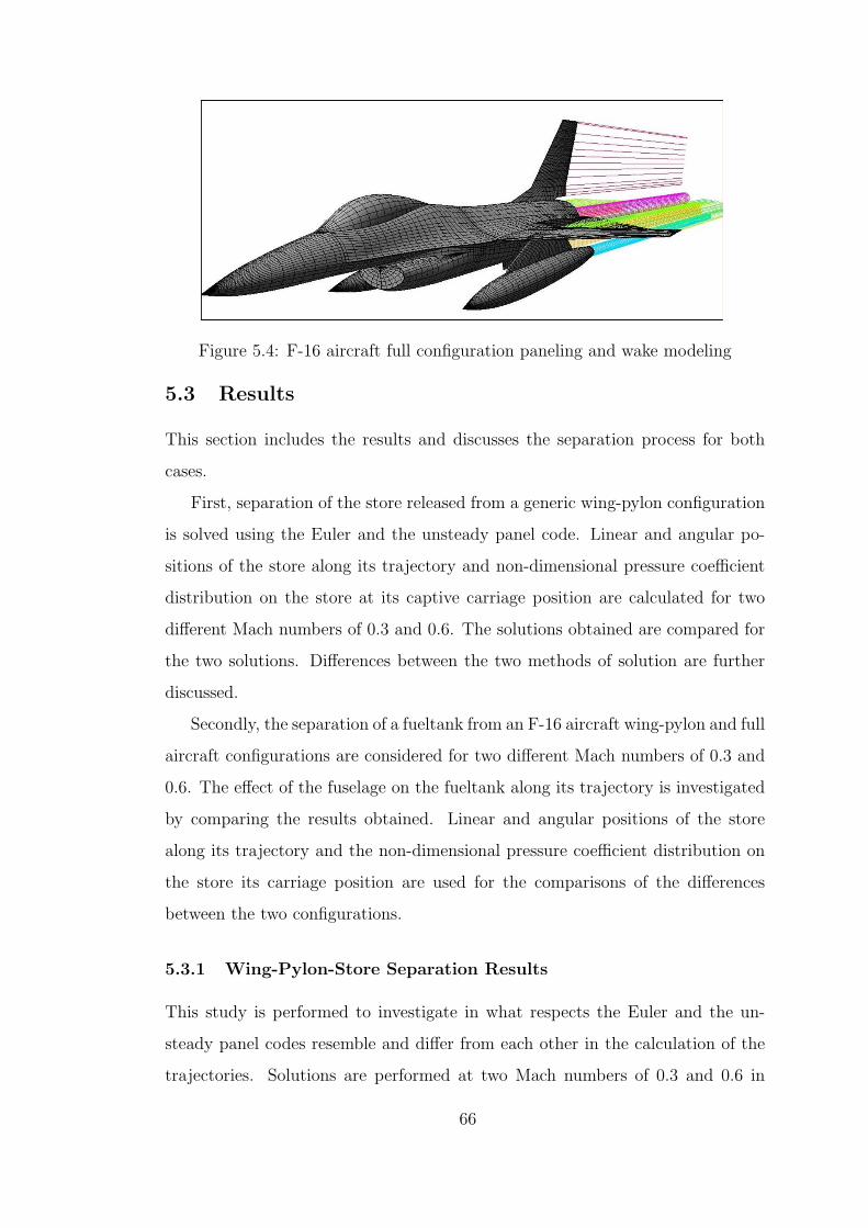
Figure 5.4: F-16 aircraft full configuration paneling and wake modeling

5.3 Results

This section includes the results and discusses the separation process for both

cases.

First, separation of the store released from a generic wing-pylon configuration

is solved using the Euler and the unsteady panel code. Linear and angular po-

sitions of the store along its trajectory and non-dimensional pressure coefficient

distribution on the store at its captive carriage position are calculated for two

different Mach numbers of 0.3 and 0.6. The solutions obtained are compared for

the two solutions. Differences between the two methods of solution are further

discussed.

Secondly, the separation of a fueltank from an F-16 aircraft wing-pylon and full

aircraft configurations are considered for two different Mach numbers of 0.3 and

0.6. The effect of the fuselage on the fueltank along its trajectory is investigated

by comparing the results obtained. Linear and angular positions of the store

along its trajectory and the non-dimensional pressure coefficient distribution on

the store its carriage position are used for the comparisons of the differences

between the two configurations.

5.3.1 Wing-Pylon-Store Separation Results

This study is performed to investigate in what respects the Euler and the un-

steady panel codes resemble and differ from each other in the calculation of the

trajectories. Solutions are performed at two Mach numbers of 0.3 and 0.6 in

66

+ + ++

++

++

+

+

+

+

+

+

+

+

+

+

+

+

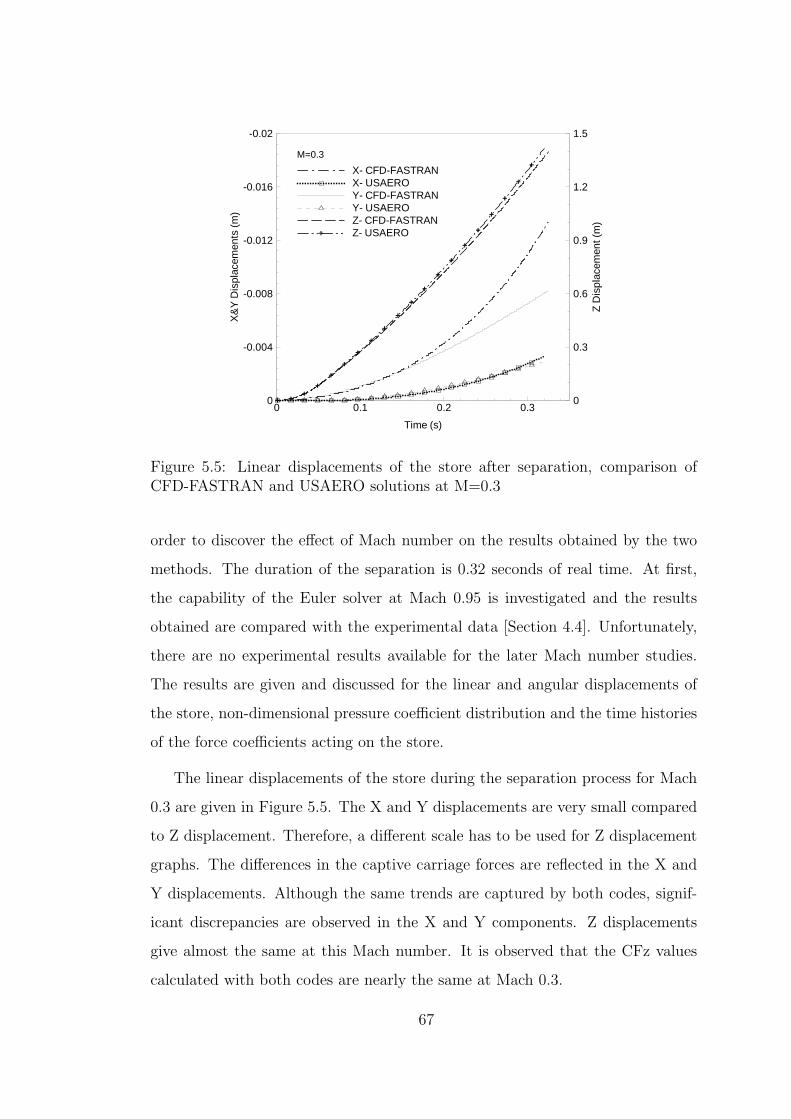
Time (s)

X&

YD

ispl

acem

ents

(m)

ZD

ispl

acem

ent(

m)

0 0.1 0.2 0.3

-0.02

-0.016

-0.012

-0.008

-0.004

0 0

0.3

0.6

0.9

1.2

1.5

X- CFD-FASTRANX- USAEROY- CFD-FASTRANY- USAEROZ- CFD-FASTRANZ- USAERO+

M=0.3

Figure 5.5: Linear displacements of the store after separation, comparison ofCFD-FASTRAN and USAERO solutions at M=0.3

order to discover the effect of Mach number on the results obtained by the two

methods. The duration of the separation is 0.32 seconds of real time. At first,

the capability of the Euler solver at Mach 0.95 is investigated and the results

obtained are compared with the experimental data [Section 4.4]. Unfortunately,

there are no experimental results available for the later Mach number studies.

The results are given and discussed for the linear and angular displacements of

the store, non-dimensional pressure coefficient distribution and the time histories

of the force coefficients acting on the store.

The linear displacements of the store during the separation process for Mach

0.3 are given in Figure 5.5. The X and Y displacements are very small compared

to Z displacement. Therefore, a different scale has to be used for Z displacement

graphs. The differences in the captive carriage forces are reflected in the X and

Y displacements. Although the same trends are captured by both codes, signif-

icant discrepancies are observed in the X and Y components. Z displacements

give almost the same at this Mach number. It is observed that the CFz values

calculated with both codes are nearly the same at Mach 0.3.

67

+ + ++

++

++

++

++

++

+

+

+

+

+

+

Time (s)

X&

YD

ispl

acem

ents

(m)

ZD

ispl

acem

ent(

m)

0 0.1 0.2 0.3

-0.04

-0.032

-0.024

-0.016

-0.008

0 0

0.3

0.6

0.9

1.2

1.5

X- CFD-FASTRANX- USAEROY- CFD-FASTRANY- USAEROZ- CFD-FASTRANZ- USAERO+

M=0.6

Figure 5.6: Linear displacements of the store after separation,comparison of CFD-FASTRAN and USAERO solutions at M=0.6

The linear displacements of the store during separation process for Mach 0.6

are given in Figure 5.6. The X and Y displacements are four times larger than

the values for Mach 0.3 results, but still they are very small when compared with

the Z displacement. Z displacements are very close to each other as it was for

Mach 0.3 case.

Angular orientations can be seen in Figures 5.7 and 5.8 for Mach 0.3 and 0.6,

respectively. Yaw and roll angles are small when compared with the pitch angle.

Therefore, a different scale had to be used for pitch angle displacement. Yaw and

roll angles have the same trends for both Mach numbers. However, pitch angle

variations for Euler solutions has different trends for the two Mach numbers.

Store pitch angle continuously increases at low Mach number. For Mach 0.6,

pitch angle change rate decreases at the end of the simulation. This attitude

of the store is similar to the Mach 0.95 solution. The pitching moment due to

aerodynamic forces starts to take the control after the ejection forces disappear.

The largest discrepancy is observed in the roll angle predictions by both of

the codes at the given Mach numbers, whereas the predictions for the yaw angles

by both of the codes are in better agreement. This agreement is getting better

with increasing Mach number.

68

+ ++

+

+

+

+

+

+

+

+

+

+

+

+

+

+

+

+

Time (s)

Yaw

&R

oll(

deg)

Pitc

h(d

eg)

0 0.1 0.2 0.30

0.09

0.18

0.27

0.36

0

4

8

12

16

20

CFD-FASTRAN- Yaw (+ towards outboard)USAERO- YawCFD-FASTRAN- Roll (+ towards outb.)USAERO- RollCFD-FASTRAN- Pitch (+ upwards)USAERO- Pitch+

M=0.3

Figure 5.7: Angular displacements of the store with respect to its body axis afterseparation, comparison of CFD-FASTRAN and USAERO solutions at Mach 0.3

+ ++

+

+

+

+

+

+

+

+

+

+

+

+

+

++

++

Time (s)

Yaw

&R

oll(

deg)

Pitc

h(d

eg)

0 0.1 0.2 0.30

0.36

0.72

1.08

1.44

0

4

8

12

16

20

CFD-FASTRAN- Yaw (+ towards outboard)USAERO- YawCFD-FASTRAN- Roll (+ towards outboard)USAERO- RollCFD-FASTRAN- Pitch (+ upwards)USAERO- Pitch+

M=0.6

Figure 5.8: Angular displacements of the store with respect to its body axis afterseparation, comparison of CFD-FASTRAN and USAERO solutions at Mach 0.6

69

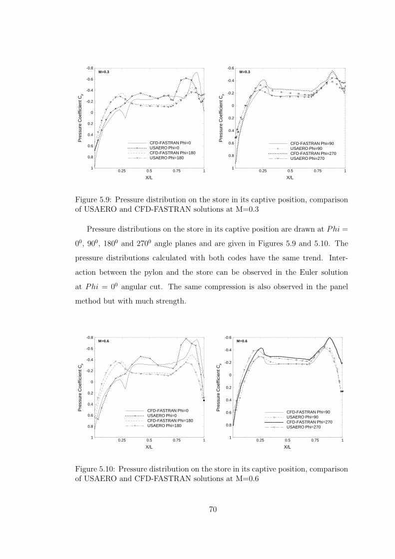
X/L

Pre

ssur

eC

oeff

icie

ntC

p

0.25 0.5 0.75 1

-0.8

-0.6

-0.4

-0.2

0

0.2

0.4

0.6

0.8

1

CFD-FASTRAN Phi=0USAERO Phi=0CFD-FASTRAN Phi=180USAERO Phi=180

M=0.3

X/L

Pre

ssur

eC

oeff

icie

ntC

p

0.25 0.5 0.75 1

-0.6

-0.4

-0.2

0

0.2

0.4

0.6

0.8

1

CFD-FASTRAN Phi=90USAERO Phi=90CFD-FASTRAN Phi=270USAERO Phi=270

M=0.3

Figure 5.9: Pressure distribution on the store in its captive position, comparisonof USAERO and CFD-FASTRAN solutions at M=0.3

Pressure distributions on the store in its captive position are drawn at Phi =

00, 900, 1800 and 2700 angle planes and are given in Figures 5.9 and 5.10. The

pressure distributions calculated with both codes have the same trend. Inter-

action between the pylon and the store can be observed in the Euler solution

at Phi = 00 angular cut. The same compression is also observed in the panel

method but with much strength.

X/L

Pre

ssur

eC

oeff

icie

ntC

p

0.25 0.5 0.75 1

-0.8

-0.6

-0.4

-0.2

0

0.2

0.4

0.6

0.8

1

CFD-FASTRAN Phi=0USAERO Phi=0CFD-FASTRAN Phi=180USAERO Phi=180

M=0.6

X/L

Pre

ssur

eC

oeff

icie

ntC

p

0.25 0.5 0.75 1

-0.6

-0.4

-0.2

0

0.2

0.4

0.6

0.8

1

CFD-FASTRAN Phi=90USAERO Phi=90CFD-FASTRAN Phi=270USAERO Phi=270

M=0.6

Figure 5.10: Pressure distribution on the store in its captive position, comparisonof USAERO and CFD-FASTRAN solutions at M=0.6

70

++ +

+ + + + + + + + + + + + ++ + + +

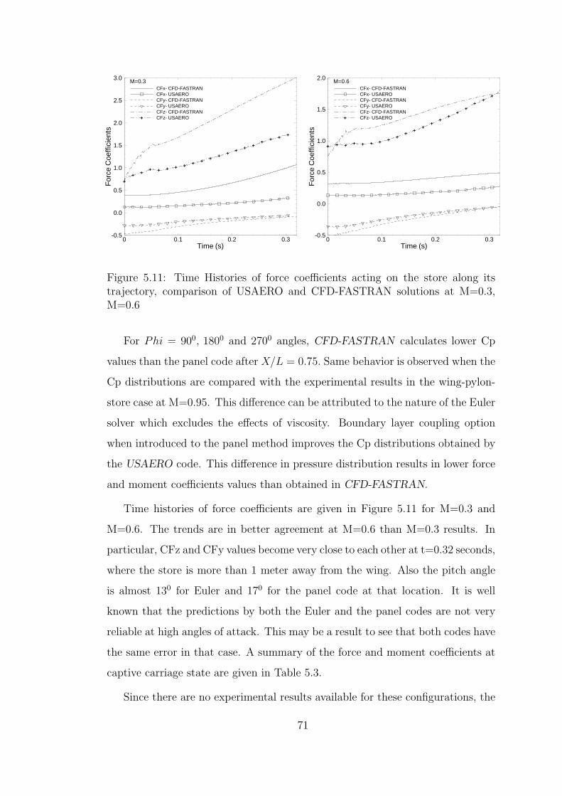
Time (s)

For

ceC

oeff

icie

nts

0 0.1 0.2 0.3-0.5

0.0

0.5

1.0

1.5

2.0

2.5

3.0

CFx- CFD-FASTRANCFx- USAEROCFy- CFD-FASTRANCFy- USAEROCFz- CFD-FASTRANCFz- USAERO+

M=0.3

+ + + + + + + + ++

++

++

++

++

++

Time (s)

For

ceC

oeff

icie

nts

0 0.1 0.2 0.3-0.5

0.0

0.5

1.0

1.5

2.0

CFx- CFD-FASTRANCFx- USAEROCFy- CFD-FASTRANCFy- USAEROCFz- CFD-FASTRANCFz- USAERO+

M=0.6

Figure 5.11: Time Histories of force coefficients acting on the store along itstrajectory, comparison of USAERO and CFD-FASTRAN solutions at M=0.3,M=0.6

For Phi = 900, 1800 and 2700 angles, CFD-FASTRAN calculates lower Cp

values than the panel code after X/L = 0.75. Same behavior is observed when the

Cp distributions are compared with the experimental results in the wing-pylon-

store case at M=0.95. This difference can be attributed to the nature of the Euler

solver which excludes the effects of viscosity. Boundary layer coupling option

when introduced to the panel method improves the Cp distributions obtained by

the USAERO code. This difference in pressure distribution results in lower force

and moment coefficients values than obtained in CFD-FASTRAN.

Time histories of force coefficients are given in Figure 5.11 for M=0.3 and

M=0.6. The trends are in better agreement at M=0.6 than M=0.3 results. In

particular, CFz and CFy values become very close to each other at t=0.32 seconds,

where the store is more than 1 meter away from the wing. Also the pitch angle

is almost 130 for Euler and 170 for the panel code at that location. It is well

known that the predictions by both the Euler and the panel codes are not very

reliable at high angles of attack. This may be a result to see that both codes have

the same error in that case. A summary of the force and moment coefficients at

captive carriage state are given in Table 5.3.

Since there are no experimental results available for these configurations, the

71

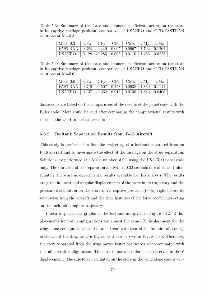
Table 5.3: Summary of the force and moment coefficients acting on the storein its captive carriage position, comparison of USAERO and CFD-FASTRANsolutions at M=0.3

Mach 0.3 CFx CFy CFz CMx CMy CMzFASTRAN 0.384 -0.449 0.695 0.0967 1.702 0.1261USAERO 0.128 -0.285 0.695 0.0110 1.465 0.0225

Table 5.4: Summary of the force and moment coefficients acting on the storein its captive carriage position, comparison of USAERO and CFD-FASTRANsolutions at M=0.6

Mach 0.6 CFx CFy CFz CMx CMy CMzFASTRAN 0.319 -0.507 0.758 0.0938 1.839 0.1111USAERO 0.137 -0.362 0.912 0.0130 1.882 0.0406

discussions are based on the comparisons of the results of the panel code with the

Euler code. More could be said after comparing the computational results with

those of the wind-tunnel test results

5.3.2 Fueltank Separation Results from F-16 Aircraft

This study is performed to find the trajectory of a fueltank separated from an

F-16 aircraft and to investigate the effect of the fuselage on the store separation.

Solutions are performed at a Mach number of 0.3 using the USAERO panel code

only. The duration of the separation analysis is 0.32 seconds of real time. Unfor-

tunately, there are no experimental results available for this analysis. The results

are given in linear and angular displacements of the store in its trajectory and the

pressure distribution on the store in its captive position (t=0 s) right before its

separation from the aircraft and the time histories of the force coefficients acting

on the fueltank along its trajectory.

Linear displacement graphs of the fueltank are given in Figure 5.12. Z dis-

placements for both configurations are almost the same. X displacement for the

wing alone configuration has the same trend with that of the full aircraft config-

uration, but the drag value is higher as it can be seen in Figure 5.15. Therefore,

the store separated from the wing moves faster backwards when compared with

the full aircraft configuration. The most important difference is observed in the Y

displacement. The side force calculated on the store in the wing alone case is very

72

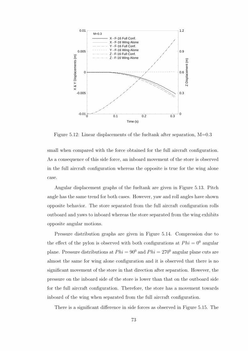
Time (s)

X&

YD

ispl

acem

ents

(m)

ZD

ispl

acem

ent(

m)

0 0.1 0.2 0.3-0.01

-0.005

0

0.005

0.01

0

0.3

0.6

0.9

1.2

X - F-16 Full Conf.X - F-16 Wing AloneY - F-16 Full Conf.Y - F-16 Wing AloneZ - F-16 Full Conf.Z - F-16 Wing Alone

M=0.3

Figure 5.12: Linear displacements of the fueltank after separation, M=0.3

small when compared with the force obtained for the full aircraft configuration.

As a consequence of this side force, an inboard movement of the store is observed

in the full aircraft configuration whereas the opposite is true for the wing alone

case.

Angular displacement graphs of the fueltank are given in Figure 5.13. Pitch

angle has the same trend for both cases. However, yaw and roll angles have shown

opposite behavior. The store separated from the full aircraft configuration rolls

outboard and yaws to inboard whereas the store separated from the wing exhibits

opposite angular motions.

Pressure distribution graphs are given in Figure 5.14. Compression due to

the effect of the pylon is observed with both configurations at Phi = 00 angular

plane. Pressure distributions at Phi = 900 and Phi = 2700 angular plane cuts are

almost the same for wing alone configuration and it is observed that there is no

significant movement of the store in that direction after separation. However, the

pressure on the inboard side of the store is lower than that on the outboard side

for the full aircraft configuration. Therefore, the store has a movement towards

inboard of the wing when separated from the full aircraft configuration.

There is a significant difference in side forces as observed in Figure 5.15. The

73

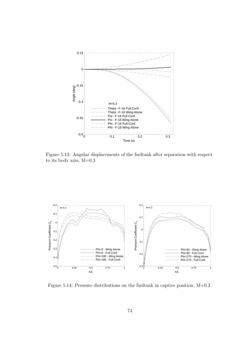
Time (s)

Ang

le(d

eg)

0 0.1 0.2 0.3-0.6

-0.45

-0.3

-0.15

0

0.15

Theta - F-16 Full Conf.Theta - F-16 Wing AlonePsi - F-16 Full Conf.Psi - F-16 Wing AlonePhi - F-16 Full Conf.Phi - F-16 Wing Alone

M=0.3

Figure 5.13: Angular displacements of the fueltank after separation with respectto its body axis, M=0.3

X/L

Pre

ssur

eC

oeff

icie

ntC

p

0 0.25 0.5 0.75 1

-0.2

-0.1

0

0.1

0.2

0.3

0.4

0.5

Phi=0 - Wing AlonePhi=0 - Full Conf.Phi=180 - Wing AlonePhi=180 - Full Conf.

M=0.3

X/L

Pre

ssur

eC

oeff

icie

ntC

p

0 0.25 0.5 0.75 1

-0.2

-0.1

0

0.1

0.2

0.3

Phi=90 - Wing AlonePhi=90 - Full Conf.Phi=270 - Wing AlonePhi=270 - Full Conf.

M=0.3

Figure 5.14: Pressure distributions on the fueltank in captive position, M=0.3

74

Time (s)

For

ceC

oeff

icie

nts,

CF

x,C

Fy,

CF

z

0 0.1 0.2 0.3-0.08

-0.06

-0.04

-0.02

0

0.02

0.04

0.06

0.08

0.1

0.12CFx - F-16 Full Conf.CFx - F-16 Wing AloneCFy - F-16 Full Conf.CFy - F-16 Wing AloneCFz - F-16 Full Conf.CFz - F-16 Wing Alone

M=0.3

Figure 5.15: Time histories of force coefficients acting on the fueltank along itstrajectory, M=0.3

negative side force on the store when released from the full aircraft configuration

shows a linear decrease as the store moves downwards. This result shows the pre-

dominant effect of including the fuselage to the modeling of a fueltank separation

problem. Also an increase in the lift and a decrease in the drag coefficient acting

on the store are also observed. A summary of the force and moment coefficients

at the captive carriage state are given in Table 5.5.

The results show that wing alone solutions for the fueltank separation can not

be substituted for full aircraft solutions. The displacements of the fueltank will

increase and become more important at higher Mach numbers.

Table 5.5: Summary of the force and moment coefficients acting on the fueltankin its captive carriage position right before separation, M=0.3

Fueltank CFx CFy CFz CMx CMy CMzWing Conf. 0.0506 0.0044 0.0314 0.0004 -0.7359 -0.0021Full Conf. 0.0427 -0.0823 0.0664 0.0034 -0.7585 -0.0517

75

CHAPTER 6

CONCLUDING REMARKS

In this thesis, store separation from two different aircraft configurations are

solved using commercially available CFD codes; CFD-FASTRAN an implicit Eu-

ler solver and an unsteady panel method solver USAERO, coupled with integral

boundary layer solution procedure. Euler solutions are obtained using chimera

methodology. The computational results are validated against the available ex-

perimental data of a generic wing-pylon-store configuration at Mach 0.95. Same

configuration is used for the comparison of unsteady panel method with Euler

solution at Mach 0.3 and 0.6. Trajectories of a fueltank separated from an F-16

aircraft wing and full aircraft configurations are solved at Mach 0.3 using only

the unsteady panel code the effect of the fuselage is observed on the trajectories

and angular orientations of the fueltank.

Preliminary studies are performed in order to test the capabilities of CFD-

FASTRAN flow solver, the chimera algorithm and the 6DOF body motion mod-

ule. The first case is the steady state solution of the store alone configuration and

two stores side-by-side cases at Mach 0.95. The store grids and the background

grid are created independently and chimera methodology is used in the solution

process. The pressure coefficient distribution on the store is compared with the

available experimental data. Both the pressure distribution on store alone and

two stores side-by-side cases show a very good agreement with the experimen-

tal data. This shows that even there is an interaction between two bodies, the

76

chimera methodology works fine with the Euler solver.

The second case is the steady state Euler solution of the wing-store configu-

ration. CFD-FASTRAN solution is compared with another Euler solver [33]. In

order to eliminate the grid dependency, same grids are used in the solution using

both codes. Mach number is taken as 0.95 and chimera methodology is used with

both codes. Pressure distributions on the wing surface at two different spanwise

locations and store surface at 4 axial cuts are compared with each other. All the

pressure distribution trends are the same on both wing and the store. Shocks are

found almost at the same locations with both codes. However, the Euler code

[33] smoothes the Cp curves at the shock locations due to its dissipative terms

and CFD-FASTRAN calculates the shock locations more accurately.

The third case is the store separation test case using the generic wing-pylon-

finned store configuration. The linear and angular displacements and velocities

of the store is compared with the available experimental results [8]. The time

history of force coefficients and the pressure distribution on the store at four

different angular cuts are also used for the comparison purposes. Preliminary

study on the number of cells to be used for the interpolation between the store

and the pylon show that the pressure distribution on the store is highly effected

with this grid node number.

All major trends of the linear and angular displacements and velocities are

captured using the chimera methodology. Store moves backward, downward and

towards inboard after separation. There are some discrepancies from the exper-

imental data. The main difference between the calculated force coefficients and

the available data is seen at Cz value. However, all the trends in forces, velocities

and displacements graphs support each other.

The error is introduced to the results since the effect of viscosity is neglected

using the Euler equations. The ejector forces are not modeled correctly, since they

are not recorded during the experiments. This approximation on these forces may

affect the results. Also the experiment results are not time accurate since CTS

technique was used in the experiments, which is a quasisteady method. The

time accurate computations are performed during the solution process, therefore

77

error could be introduced to the results. Since the sting is mounted behind

the store in the experiments, a correction base force is applied on the store in

numeric computations. Otherwise, high drag values are obtained and this would

yield wrong displacements in the axial direction. Despite all these errors, from

the results obtained so far, the CFD-FASTRAN solver can be used in the store

separation problems.

The possible effects of the sting on the trajectory characteristics are also

investigated. For this purpose, the sting is unmounted from the store and the

store base is smoothed as its nose shape. The calculations are repeated at Mach

0.95.

It is seen that the linear displacements are not affected except the axial dis-

placement. The axial displacements are higher than the experimental data since

the base of the store is not the same as used in the experiments. Also no base

force correction is used for the solutions. Therefore, this result is as expected.

Better trajectory results are obtained in pitching and yawing motions. Linear

velocity curves are not affected much. However, higher roll rate values are cal-

culated when the base of the store is smoothed. This results in higher roll angle

displacements than the experimental data and the previous solution with the

sting. Pitch and yaw angle rates are in better agreement with the experimental

data until t=0.25 seconds. Side force coefficient histories for both configurations

are the same. However, the force component in the z direction has better coher-

ence with the experimental data. But this improvement on the force coefficient is

not reflected to the z displacements. This shows that the store moves downward

under the effect of the inertial forces. Axial force values of the store are in better

agreement with the experimental data after 0.2 seconds. This is the result of

weaker interaction between the store and the wing-pylon, which highly affects

the axial force calculations.

Two different store separation cases are studied. The first case is the separa-

tion of a finned store from wing-pylon configuration. This configuration is solved

both with the Euler and unsteady panel codes at Mach numbers of 0.3 and 0.6.

The aim is to compare the two methods of prediction tools and to find out which

78

aspects of store separation phenomenon could be captured.

Due to the weight of the store and the ejector forces, X and Y displacements

of the store are very small compared to the Z displacement of the store at both

Mach numbers. Z displacements of the store are the same when calculated with

both codes. But axial and lateral displacements found by using the Euler code

are more than twice as large as the panel code solutions. However, depending on

the separation criteria, these displacements can be neglected since they are very

small.

Increase in Mach number increases the magnitudes of axial and lateral dis-

placements but do not effect the downward displacement. This shows that the

store is displaced under the effects of inertial forces. All the trends of the curves

are the same.

Yaw and roll angles are small compared to pitch angle for both Mach numbers.

Yaw and roll angles have the same trends using the both codes for both Mach

numbers, but the pitch angle variations differs for Euler solution at Mach 0.6.

The trend of the curve shows that aerodynamic forces start to take the control

of the store trajectory at Mach 0.6.

The compression due to pylon at carriage position is observed with both codes

but panel code calculates much in weaker strength. Boundary layer coupling op-

tion improves the pressure distribution obtained by the panel code. The trends

of the pressure distributions are the same but the differences between the mag-

nitudes starts after the fin location, where viscous effects are dominated.

Force coefficient histories of the store are in better agreement at high Mach

number. Since no experimental results available, discussions are based on the

comparison of the results of the panel code with the Euler code.

The second case is the separation of a fueltank from an F-16 aircraft wing-

alone and full aircraft configurations at Mach number 0.3. The aim is to in-

vestigate the fuselage effect on the trajectory of the fueltank after separation.

Solutions are obtained using the unsteady panel code.

The fuselage does not have any significant effect on the downward displace-

ment of the fueltank in this configuration. Higher drag value is obtained in full

79

aircraft configuration than wing alone case, therefore the store moves faster to-

wards the backward. The fuselage affects the side force exerted on the fueltank,

and fueltank moves inboard after separation whereas the opposite is true for wing

alone case. Also, the fuselage affects the roll and yaw motion of the fueltank and

these directions are reversed.

The modeling of a full aircraft configuration for the Euler solution using struc-

tured grids is a challenge. Instead of modelling the full aircraft configuration, one

can model only the wing of the aircraft and perform the solutions. However, the

results shows that the wing is not a substitude for the fuselage. The compressed

flow between the fuselage and the store highly affects the attitude of the store.

This effect will be higher and becomes critical at high Mach numbers.

The same configuration can be modelled in less time and effort for a panel

code than an Euler/Navier-Stokes solver. All the cases in the solution matrix

using a panel code can be performed in a solution time needed for a unique Euler

solution. However, solutions at high Mach numbers, which are close to transonic

regimes must be obtained using a compressible Euler or Navier/Stokes solver.

Further research is also in progress for the store separation from wing-pylon-

store configuration at Mach 1.2. The results will be validated with the available

experimental data. Also, ACFD Challenge II configuration F-18/C with JDAM

is obtained and will be modelled in CFD-GEOM using structured grids. The

results will be compared with the available flight test data.

80

REFERENCES

[1] Schindel, Leon H., Store Separation, AGARD-AG-202, 1975.

[2] Cenko, A., Experience in the use of computational aerodynamics to predictstore release characteristics, Progress in Aerospace Sciences, 37 (2001), pp477-495.

[3] Cenko A, Tinoco EN, PAN AIR - weapons, carriage and separation. AFFDL-TR-79-3142, December 1979.

[4] Meyer R, Cenko A, Yaros S., An influence function method for predictingaerodynamic characteristics during weapon separation, 12th Navy Sympo-sium on Aeroballistics, May 1981.

[5] Nielsen JN. et al. A calculative method for predicting store separation trajec-tories at speeds up to the critical speed, AGARD-CP-71, January 1971.

[6] Steger JL., Dougherty FC., Benek JA., A Chimera grid scheme, Advancesin grid generation, ASME, June 1983.

[7] Lohner R., Adaptive remeshing for transient problems with moving bodies,AIAA Paper 88-3736, 1988.

[8] Fox., J. H., 23. Generic Wing, Pylon, and Moving Finned Store, Verificationand Validation Data for Computational Unsteady Aerodynamics, RTO-TR-26, October 2000, St. Joseph Ottawa/Hill, Canada.

[9] Newman JC, Baysal O., Transonic Solutions of a Wing/Pylon/Finned storeusing hybrid domain decomposition, AIAA Paper 92-4571, August 1992.

[10] Parikh P, Pirzadeh S, Frink NT., Unstructured grid solutions to aWing/Pylon/Store configuration using VGRID3D/USM3D, AIAA Paper 92-4572, August 1992

[11] Meakin R., Computations of the unsteady viscous flow about a genericWing/Pylon/Finned-Store configuration, AIAA Paper 92-4568, August 1992.

[12] Madson M. et al. TranAir computations of the flow about a GenericWing/Pylon/Finned-store configuration, AIAA Paper 94-0155, January 1994

[13] Demir, H.O., Alemdaroglu, N., Ucak Kanadından Harici Yuk Ayrılması,Savunma Teknolojileri Kongresi, 24-25 Haziran 2004, Ankara.

81

[14] Madson M, Talbot M., F-16/Generic store carriage load predictions at tran-sonic Mach numbers using TranAir, AIAA-96-2454, June, 1996

[15] Wey T., Martin F., Application of the OVERFLOW code to the F-16 con-figuration, AIAA-96-2459, June 1996.

[16] Chine D. et al. Calculation of generic store separation from an F-16 Aircraft,AIAA-96-2455, June 1996.

[17] Cenko, A. et al., F/A-18C/JDAM CFD Challenge results /ACFD ChallengeII AIAA paper 2000-0795, January 2000.

[18] Rock, S.G., and Habchi, S.D., Yeiser, C., and Oslon, M., Marwuette, T., AComputational Methodology for the Rapid Simulation of Jettisoned AircraftCanopy Trajectories, 35th Aerospace Sciences Meeting and Exhibit, January6-10, 1997.

[19] Hall., L., Navier-Stokes /6-DOF Analysis of the JDAM store separation fromthe F/A-18C Aircraft, AIAA Paper 99-0122, January 1999.

[20] Chen., P.C., Liu., D.D., Store-Separation Analyses at Subsonic and Super-sonic Speeds Using a High-Order Panel Method, AGARD 76th Fluid Dynam-ics Panel Meeting and Symposium on Aerodynamics of Store Integration andSeparation, Ankara, Turkey, 24-28 April, 1995.

[21] Lijewski, L. E., and Suhs, N. E., Time-Accurate Computational Fluid Dy-namics Approach to Transonic Store Separation Trajectory Prediction, Jour-nal of Aircraft, Vol. 31. No. 4, 1994, pp. 886-891.

[22] Prewitt, N. C., Belk, D.M., and Maple, R. C., Multiple Body Trajectorycalculations Using the Beggar Code, Journal of Aircraft, Vol. 36, No. 5, 1999,pp. 802-808.

[23] Lee, S., and Park, M., Cho, K. W., and Kwon, J. H., New Fully AutomatedProcedure for the Prediction of Store Trajectory, Journal of Aircraft, Vol. 37,No. 6, 2000.

[24] Demir, H.O., Alemdaroglu, N., Ucak Kanadından Harici Yuk Ayrılması,Kayseri V. Havacılık Sempozyumu, 13-14 Mayıs 2004, Kayseri

[25] Demir, H.O., Alemdaroglu, N., External Store Separation from Fighter Air-craft, AVT-108, Symposium on ”Functional and Mechanical Integration ofWeapons with Land and Air Vehicles,” 7-10 June 2004 Williamsburg, VA,UNITED STATES

[26] Kern, S.B.,Findlay, D.B., F/A-18C Store Carriage Loads Prediction andMutual Interference Aerodynamics, presented in RTO SCI Symposium onAircraft Weapon System Compatibility and Integration, Chester, UK, 28-30September 1998

82

[27] Wang, Z.J., Yang, H.Q., A Unified Conservative Zonal Interface Treat-ment for Arbitrarily Patched and Overlapped Grids, 32nd Aerospace SciencesMeeting and Exhibit, January 10-13, 1994, /Reno, NV

[28] Wang, Z.J., A fully Conservative Structured/Unstructured Chimera GridScheme, 33rd Aerospace Sciences Meeting and Exhibit, January 9-12, 1995/Reno, NV

[29] Wang, Z.J., Buning, P., Benek, J., Critical Evaluation of Conservative andNon-Conservative Interface Treatment for Chimera Grids, 33rd AerospaceSciences Meeting and Exhibit, January 9-12, 1995 /Reno, NV

[30] Wang, Z.J., A Conservative Overlapped (Chimera)Grid Algoritm for MultipleBody Flows, 34th Aerospace Sciences Meeting and Exhibit, January 15-18,1996 /Reno, NV

[31] CFD-FASTRAN Theory Manual, Version 2003, CFDRC Research Corpora-tion, May 2003.

[32] Lijewski L.E., Transonic Euler Solutions on Mutually Interfering FinnedBodies, AIAA Journal, Vol., 28, No. 6

[33] Tarhan E., Two and Three Dimensional Overset Grid Solutions ofEuler/Navier-Stokes Equations, PHD Thesis, METU, July 2003

[34] Kurtulus D.F., Aerodynamic Analysis of a Full Aircraft Configuration Usinga Panel Method, M.S. Thesis, METU, January 2002

[35] Bozkurttas M., Aerodynamic Analysis of External Stores on Aircraft, M.S.Thesis, METU, November 2001

[36] Erhan H., Aerodynamic Analysis of Fighter Aircraft F-16 With ExternalStores, M.S. Thesis, METU, January 2003

83