computational design, sensitivity analysis and
TRANSCRIPT
COMPUTATIONAL DESIGN, SENSITIVITY ANALYSIS AND OPTIMIZATION OF FUEL REFORMING CATALYTIC REACTOR
By
Arman Raoufi
James C. Newman III Sagar Kapadia Professor of Computational Engineering Research Assistant Professor of (Chair) Computational Engineering (Committee Member)
Robert S. Webster James Hiestand Research Associate Professor of Professor of Mechanical Engineering Computational Engineering (Committee Member) (Committee Member)

ii
COMPUTATIONAL DESIGN, SENSITIVITY ANALYSIS AND OPTIMIZATION OF FUEL REFORMING CATALYTIC REACTOR
By
Arman Raoufi
A Dissertation Submitted to the Faculty of the University of Tennessee at Chattanooga in Partial Fulfillment
of the Requirements of the Degree of Doctor of Philosophy in Computational Engineering
The University of Tennessee at Chattanooga Chattanooga, Tennessee
August 2016

iii
Copyright © 2016
By Arman Raoufi
All Rights Researved

iv
ABSTRACT
In this research, the catalytic combustion of methane is numerically investigated using an
unstructured, implicit, fully coupled finite volume approach. The nonlinear system of equations
is solved by Newton’s method. The catalytic partial oxidation of methane over a rhodium
catalyst in one channel of a coated honeycomb reactor is studied three-dimensionally, and eight
gas-phase species (CH4, CO2, H2O, N2, O2, CO, OH and H2) are considered for the simulation.
Surface chemistry is modeled by detailed reaction mechanisms including 38 heterogeneous
reactions with 20 surface-adsorbed species for the Rh catalyst and 24 heterogeneous reactions
with 11 surface-adsorbed species for Pt catalyst. The numerical results are compared with
experimental data and good agreement is observed. Effects of the design variables, which
include the inlet velocity, methane/oxygen ratio, catalytic wall temperature, and catalyst loading
on the cost functions representing methane conversion and hydrogen production are numerically
investigated. The sensitivity analysis for the reactor is performed using three different
approaches: finite difference, direct differentiation and an adjoint method. Two gradient-based
design optimization algorithms are utilized to improve the reactor performance. For additional
test cases, the performance of two full scale honeycomb-structured reactors with 49 and 261
channels are investigated. The sensitivity analysis of the full reactor is performed using an
adjoint method with four design variables consisting of the inlet velocity, inflow methane
concentration, inlet oxygen density and thermal conductivity of the monolith.

v
DEDICATION
This dissertation is lovingly dedicated to my mother, Zahra Ghorbannejad, who passed
away in November, 2015 and could not see this dissertation completed, for her lifetime support,
encouragement, and unbounded love.

vi
ACKNOWLEDGMENTS
My deepest gratitude goes to my beautiful wife Maryam for her support, encouragement,
kindness and unbounded love and my lovely sweet daughter Ava.
I would like to express my special appreciation and thanks to my advisor Dr. James
Newman for devoting a great deal of time to answer my questions and offer suggestions. I wish
to express my thanks to Dr. Sagar Kapadia for his time and effort over the past five years.
Without their guidance and encouragement throughout my time as a graduate student, this work
would not have been possible. I also thank my other committee members, Dr. Robert Webster
and Dr. James Hiestand for their guidance regarding this work. In addition, I would like to
express my appreciation to Dr. Timothy Swafford for his support and help.
This work was supported by the Office of Naval Research (ONR) Grant No. N00014-10-
1-0882 and the Tennessee Higher Education Commission (THEC) Center of Excellence in
Applied Computational Science and Engineering (CEACSE). This support is greatly appreciated.
vii
TABLE OF CONTENTS
ABSTRACT ................................................................................................................................................. iv DEDICATION .............................................................................................................................................. v ACKNOWLEDGMENTS ........................................................................................................................... vi LIST OF TABLES ....................................................................................................................................... ix LIST OF FIGURES ...................................................................................................................................... x LIST OF ABBREVIATIONS .................................................................................................................... xiii LIST OF SYMBOLS ................................................................................................................................. xiv CHAPTER
1. INTRODUCTION ................................................................................................................................. 1 2. GOVERNING EQUATIONS AND NUMERICAL SOLUTION ....................................................... 12
2. 1. Modeling the surface chemistry .................................................................................................... 17
2.1.1 Gas-phase chemistry model ................................................................................................... 19 2.1.2 Surface chemistry model ....................................................................................................... 20
2.2. Sensitivity derivatives .................................................................................................................... 28 3. NUMERICAL SIMULATION OF CATALYTIC COMBUSTION IN STAGNATION FLOW ....... 32
3. 1. Methane oxidation on a platinum surface .................................................................................. 37 3. 2. Methane oxidation on a platinum surface .................................................................................. 44
4. CATALYTIC PARTIAL OXIDATION OF METHANE ................................................................... 50
4.1. Parallel performance ...................................................................................................................... 50 4.2. Validation for the catalytic partial oxidation of methane ............................................................... 53 4.3. Parameter study .............................................................................................................................. 60 4.4. Sensitivity Analysis ....................................................................................................................... 69 4.5. Optimization .................................................................................................................................. 70
5.NUMERICAL SIMULATION A HONEYCOMB-STRUCTURED CATALYTIC REFORMING REACTOR ......... 76 5.1. Sensitivity analysis of the full reactor ........................................................................................ 87

viii
6. CONCLUSION .................................................................................................................................... 89 6.1. Summary ........................................................................................................................................ 89 6.2. Recommendations for future work ................................................................................................ 90 REFERENCES ........................................................................................................................................... 92 APPENDIX A. CANTERA FILE FOR CATALYTIC COMBUSTION OF HYDROGEN ON PALLADIUM ........... 96 B. REACTION MECHANISM FOR METHANE CATALYTIC COMBUSTION ON PLATINUM .... 101 C. REACTION MECHANISM FOR METHANE CATALYTIC COMBUSTION ON RHODIUM ..... 103 VITA ......................................................................................................................................................... 106

ix
LIST OF TABLES
1 The literature review and numerical studies were carried out in the field of the catalytic combustion ..... 8 2 Reaction mechanism for methane combustion on a Pt surface [6] .......................................................... 39
3 Reaction mechanism for iso-octane combustion on a Rh surface [12] .................................................... 46
4 Initial conditions for catalytic partial oxidation of methane .................................................................... 54
5 Baseline conditions for catalytic combustion of methane ........................................................................ 61
6 The sensitivity derivatives for the different design variables .................................................................. 70
7 Initial values and constrained bounds for the design variables ................................................................ 73
8 the number of solver and gradients calls for the optimization algorithms ............................................... 74
9 Initial conditions for fuel reforming reactor ............................................................................................ 78
10 Sensitivity derivatives of both cost functions obtained using the discrete adjoint method for the full reactor ........... 88
x
LIST OF FIGURES
1 The different kind of the catalytic reactors ................................................................................................ 2 2 Monoliths with various channel shapes [3] ................................................................................................ 3 3 Catalytic combustion monolith and physical and chemical process occurring in the monolith reformer . 4 4 Control Volume based on Median Dual .................................................................................................. 15 5 Methods for modeling the chemical reaction rate of heterogeneous reactions ........................................ 18
6 Schematic of the coupling between the gas and the surface due to transport and heterogeneous chemistry ..................... 21 7 Normalized runtimes for solving the stiff problem .................................................................................. 26 8 Data exchange between the solver and Cantera through the interface ..................................................... 28 9 The schematic of stagnation-point flow ................................................................................................... 35 10 The solution algorithm for solving the ODE equations ......................................................................... 36 11 Geometry and boundary conditions for catalytic combustion of methane on the platinum surface ...... 38 12 The comparison between the obtained numerical results with experimental data reported by [42] ...... 40 13 Velocity and temperature profiles for the surface temperature 800 K ................................................... 41 14 Effect of the surface temperature on CH4 concentration ....................................................................... 41 15 Surface site fraction for the different surface temperature ..................................................................... 42 16 Gas phase species concentrations for the surface temperature 1200 K .................................................. 43 17 Geometry and boundary conditions for catalytic combustion of iso-octane over the Rhodium surface ........................... 44 18 Effect of the surface temperature on I-C8H18 concentration ................................................................ 47 19 Surface coverages for the different surface temperature ........................................................................ 48 20 Gas phase species concentrations for the surface temperature 1100 K .................................................. 49 21 The total run times for the different number processors ........................................................................ 51

xi
22 Parallel performance using Speedup ...................................................................................................... 52 23 Grid generated for the channel of reactor .............................................................................................. 54 24 Convergence history of the solution ...................................................................................................... 55 25 Comparison between the numerical results and experimental data for the partial oxidation of methane .......................... 56 26 The mole fraction of species along symmetry axis of the reformer for both catalyst Rh and Pt .......... 57 27 Contour plots for the reactor with Platinum catalyst .......................................................................... 58 28 Contour plots for the reactor with Rhodium catalyst ............................................................................... 59 29 The comparison of the mole fraction of species along symmetry axis of the reformer ......................... 61 30 The mole fraction contour for the reactor with the inlet velocity 2 m/s ................................................. 62 31 The comparison of the mole fraction of species along symmetry axis of the reformer ........................................................... 63 32 The influence of the variation of methane/oxygen ratio on the reformer performance ......................... 64 33 The mole fraction contour for the reformer with the methane/oxygen ratio 1/3 .................................... 65 34 The influence of the variation of the catalyst loading on the reformer performance ............................. 67 35 The mole fraction contour for the reformer with Fcat/geoη 0.5 ....................................................... 68 36 The data interchange and interface between the flow solver and DAKOTA ......................................... 72 37 The comparison between the optimized conditions for methane concentration along the reactor ........ 74 38 The comparison between the base condition and the optimized condition for hydrogen concentration .................... 75 39 The cylindrical monolithic reactor with square cross-section channels ................................................. 77 40 The generated grid for the monolithic reactor........................................................................................ 77 41 The boundary conditions for the monolithic reactor and mesh cross-section ........................................ 78 42 Contours of a) Temperature b) Velocity for the reactor at test conditions 1 ......................................... 80 43 Contour plots for species mole fractions for test condition 1 a) CH4 b) CO2 c) CO d) H2 e) H2O f) O2 ................. 81 44 Contours of a) Velocity b) Temperature for the reactor at test conditions 2 ........................................ 82 45 Contour plots for species mole fractions at test conditions 2 a) CH4 b) CO2 c) CO d) H2 e) H2O f) O2 ..................... 83

xii
46 The structure of the reactor .................................................................................................................... 84 47 The mesh generated for the simulation .................................................................................................. 85 48 The boundary conditions for the simulation .......................................................................................... 85 49 Contour plots for the reactor a) O2 b) CH4 c) H2 d) CO2 e) Temperature ............................................................ 87

xiii
LIST OF ABBREVIATIONS
ATR, Auto Thermal Reforming CFD, Computational Fluid Dynamics SOFC, Solid Oxide Fuel Cell
xiv
LIST OF SYMBOLS
, Total molar mixture concentration
, Binary mass diffusion coefficient of species i into species j
, Knudsen diffusion coefficient
, Inviscid flux vector
, Viscous flux vector
, Young’s modulus
, Species internal energy
, Specific total energy (total energy per unit mass)
, Species enthalpy
, Mass diffusion flux vector for species i
, Heat transfer coefficient
, Mean molecular weight of the mixture
, Molecular weight of species j
, Diffusion molar flux
ns, Number of species
, Pressure (mixture)
, Partial pressure
Q, Conservative flow variables
xv
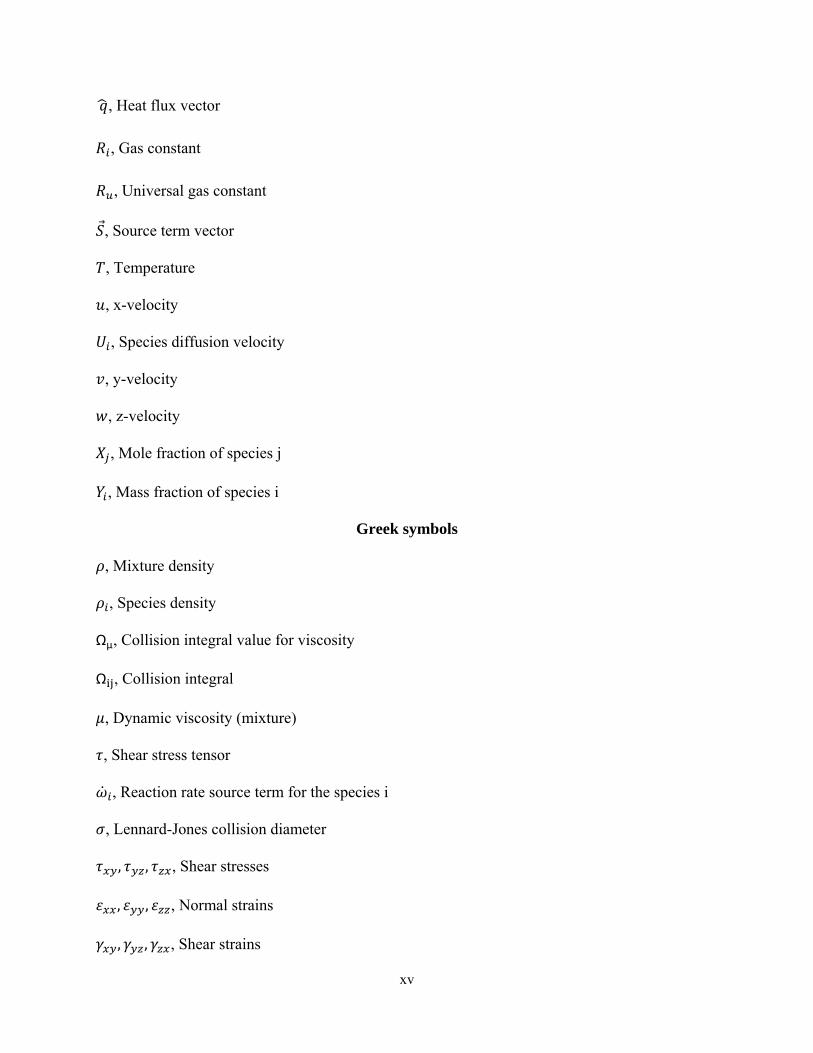
, Heat flux vector
, Gas constant
, Universal gas constant
, Source term vector
, Temperature
, x-velocity
, Species diffusion velocity
, y-velocity
, z-velocity
, Mole fraction of species j
, Mass fraction of species i
Greek symbols
, Mixture density
, Species density Ωμ, Collision integral value for viscosity Ω , Collision integral
, Dynamic viscosity (mixture) , Shear stress tensor
, Reaction rate source term for the species i
, Lennard-Jones collision diameter
, , , Shear stresses
, , , Normal strains
, , , Shear strains

xvi
, Thermal expansion coefficient
1
CHAPTER 1
INTRODUCTION
The Fuel reformer is one of the most important components of the SOFC system. The
purpose of the fuel reformer is to convert the chemical composition of primary fuel into the
species that systems like SOFCs can be operated with. Fuel reforming can be broadly classified
into three categories including, steam reforming (SR), partial oxidation (POX) and autothermal
reforming (ATR). The reactors used in reforming process can have many different structures
such as pack bed and monolith, depending on the application and other parameters. These
reactors are categorized as the catalytic reactors. Catalytic reactors are widely used in fuel
reforming processes and have engineering applications such as in automotive catalytic
converters, gas turbines, and for portable radiant heaters. There are many kinds of the catalytic
reactors used in the industry as summarized in Figure 1. These reactors are mainly required for
environment concerns with regards to reducing pollutants and emission levels. The catalytic
reactor can be distinguished from the conventional reactor by considering fundamental
differences between homogeneous (conventional) combustion and catalytic combustion. The
main differences can be summarized as [1]:
• Conventional combustion occurs in the presence of a flame, while catalytic combustion
is a flameless process.
• Catalytic combustion generally proceeds at a lower temperature than conventional
combustion.

2
• Catalytic combustion results in lower emission of oxides of nitrogen.
• Conventional combustion can only exist within well-defined fuel-to-air ratios. Catalytic
combustion is not constrained by such conditions.
• Catalytic combustion can offer fewer constraints on reactor design.
Figure 1 The different kind of the catalytic reactors
The monolith or honeycomb reactor is a commonly-used configuration in the fuel
reforming industry. With the catalyst being coated on the channel walls, these structures consist
of a number of parallel passageways through which the gas flows. The monolith configuration
offers a number of interesting features including a high surface to volume ratio with low pressure
drop that may be exploited in reactor design [1].
Monolith channels can have various cross-sectional shapes, e.g. circular, hexagonal,
Catalytic reactors
Fixed bed reactors Monolithic reactors
Wire gausesCatalytic reactors with multi-phase
fluids
Fluidized bed reactors Slurry reactors
Chemical reactors for materal synthesis
Chemical vapor deposition (CVD)
Elecro-catalytic devices

3
square or sinusoidal (Figure 2). Monolith structures can be manufactured to have a specified size
of channel, cell density, and wall thickness. Materials for the support vary ranging from ceramics
[2] to metallic alloys.
Figure 2 Monoliths with various channel shapes [3]
Catalytic monolithic reactors are generally characterized by the complex interaction of
various physical and chemical processes. Figure 3 illustrates the physics and chemistry in a
catalytic combustion monolith. The flow field includes the complex transport of momentum,
energy, and chemical species. The reactants diffuse to the inner channel wall, which is coated
with the catalytic material, where the gaseous species adsorb and react on the surface. The
products diffuse back into the flow. Since most reforming processes are conducted at high
temperatures, homogeneous reactions in the gas phase can accompany the heterogonous
reactions in the catalytic wall. In catalytic reactors, the catalyst material is often dispersed in
porous structures, such as washcoats or pellets. Mass transport in the fluid phase and chemical
reactions are then superimposed by diffusion of the species to the active catalytic centers in the
pores [2].

4
Figure 3 Catalytic combustion monolith and physical and chemical process occurring in the monolith
reformer
Because of the complexity and coupled interaction between mass and heat transfer,
design and optimization of catalytic reactors is challenging. Computational fluid dynamics
(CFD) can be used to simulate and understand the physical and chemical interactions within the
reactor. Moreover, this predictive capability may then be utilized to perform reactor design or
offer design alternatives. However, an enabling technology is the need to develop robust and
reliable numerical methods to model the fluid mechanics which includes the complex chemical

5
reactions. The use of detailed models for chemical reactions is exceedingly challenging due to
the large number of species involved, nonlinearity, and multiple time scales arising from the
complex reacting systems. The resulting partial differential equations (PDEs) tend to be very
large and stiff systems, with highly nonlinear boundary conditions [3].
In addition to design and optimization, CFD can be used to support experimental testing
of these catalytic reactors. For example, Hettel et al. (2013) developed a numerical model to
study the in situ effect of a probe insertion on the velocity and species profiles [4]. Therefore,
numerical modeling combined with experimental measurements together should be used to
provide a comprehensive and detailed understanding of catalytic reactors.
Modeling of monolithic reactors can be broadly divided in two categories: single-channel
modeling that considers just one channel of the monolith and full-scale modeling that considers
the whole reactor comprised of several hundred channels [5] [6]. Single-channel models can be
one-dimensional, two-dimensional or three-dimensional.
Simulations for a single-channel have been previously performed using one-, two- and
three-dimensional models. One-dimensional (1D) models ignore radial and angular gradients in
temperature, concentration, and velocity, and consider only axial variations. These models,
which use lumped heat and mass coefficients, are widely used because of their simplicity, ease of
implementation, and computational efficiency. The resulting one-dimensional model is typically
referred to as the plug-flow model.
In the monolith channel, the catalytic reaction occurs in the washcoat on the channel wall.
There are two choices for incorporating the catalyst reaction into the heat and mole balance
equations: pseudo-homogeneous models and heterogeneous models. In the pseudo-homogeneous
model, the wall temperature and concentrations are assumed to be the same as the fluid, and the

6
reaction rate is incorporated directly into the conservation equations. For the heterogeneous
model, the gas-solid interface at the wall is assumed to be discontinuous and separate mole and
energy balance equations are solved for the solid. These equations are coupled to the fluid
equations through mass and heat transfer coefficients. The catalytic reactor results presented in
this report utilize the heterogeneous model for surface chemistry. Since no diffusive terms
remain, the plug-flow equations form a differential-algebraic-equation (DAE) initial-value
problem for the axial variation of the mean species composition [6].
The catalytic partial oxidation of hydrogen was previously investigated by Cerkanowicz
et al. (1977) [7] with simplified chemistry and by Kramer et al. (2002) [8] with detailed kinetics.
Two and three-dimensional models are more complex but provide more realistic results than the
one-dimensional models. These models are developed based on both boundary-layer equations
and the Navier-Stokes equations. In boundary-layer approximations, axial (flow-wise) diffusive
transport is neglected, but detailed transport to and from the channel walls is retained.
Deutschmann et al. (2000) [9] and Dogwiler et al. (1999) [10] used Navier-Stokes 2D models
with detailed heterogeneous and homogeneous chemistry for simulation of the catalytic
combustion. The catalytic combustion of methane-air was studied by Markatou et al. (1993) [11]
using a 2D boundary layer model. Raja et al. (2000) [6] investigated the efficiency and validity
range of the Navier–Stokes, boundary-layer, and plug-flow models in a catalytic monolithic
channel. Their research showed that the boundary-layer models provide accurate results with low
computational cost. Kumar (2009) [5] developed a new implicit solver for species conservation
equations and investigated the flow field in a full-scale 3D catalytic converter. The catalytic
combustion of iso-octane over rhodium catalysts was studied by Hartmann et al. (2010) [12]. In
that research, detailed surface chemistry including 17 surface species and 58 surface reactions
7
was utilized in the simulation.
In the current study, the effect of considering homogeneous reaction mechanisms in the
numerical model is investigated. Maestri and Cuoci (2013) [13] have used the open-source CFD
solver OpenFOAM [15] to simulate heterogeneous catalytic systems three-dimensionally with
the detailed kinetics schemes. The catalytic partial oxidation (CPOX) of methane over a
honeycomb reactor was numerically studied by Hettel et al. (2015) [14], where OpenFOAM and
DETCHEM [17] where coupled to model a large-scale COPX reactor. Table 1 illustrates a
summary of the literature review, and presents the numerical studies that have been carried out in
the field of catalytic partial oxidation.

8
Table 1 The literature review and numerical studies were carried out in the field of the catalytic combustion
Authors Affiliation Year Model Fuel/catalyst
Cerkanowicz et al. Exxon Research and
Engineering Co 1977 1D- simplified chemistry Hydrogen- Pt
Markatou et al. Yale University 1993 2D Boundary layer-detailed
chemistry Methane -Pt
Deutschmann et al. University of Stuttgart 1994 1D- detailed chemistry Methane -Pt
Deutschmann et al. University of Heidelberg 1996 1D- detailed chemistry Methane -Pd
O. Deutschmann, L. D. Schmidt
University of Minnesota 1998 2D - detailed chemistry Methane- Rh-
Pt
Dogwiler et al. Paul Scherrer Institute 1999 2D - detailed chemistry Methane - Pt
Raja et al. Colorado School of Mines 2000 2D- detailed chemistry Methane -Pt
Deutschmann et al. University of Heidelberg 2000 2D - detailed chemistry Methane -Pt
Dupont et al. University of Leeds 2001 1D- detailed chemistry Methane -Pt
Kramer et al. University of Maryland 2002 1D- detailed chemistry Hydrogen -Pt
Minh University of Heidelberg 2005 2D- detailed chemistry-
optimization Ethane-Pt
Minh et al. Karlsruhe Institute of
Technology 2008
2D- detailed chemistry-optimization
Ethane-Pt
Kumar Ohio State University 2009 3D- detailed chemistry Methane -Pt
Hartmann et al. Karlsruhe Institute of
Technology 2010 2D- detailed chemistry Iso-octane-Rh
Maestri and Cuoci Politecnico di Milano 2013 3D- detailed chemistry Iso-octane-Rh
Hettel et al. Karlsruhe Institute of
Technology 2013 3D - detailed chemistry Methane - Rh
Hettel et al. Karlsruhe Institute of
Technology 2015 3D- detailed chemistry Methane- Rh

9
Computational fluid dynamics (CFD) methods are generally classified as two distinct
families of schemes: pressure-based and density-based methods. The pressure-based algorithm
solves the momentum and pressure correction equations separately. The density-based solver
solves the governing equations of continuity, momentum, energy and species transport
simultaneously. In the density-based approach, the velocity field is obtained from the momentum
equations and the continuity equation is used to obtain the density field. The pressure field is
determined from the equation of state using computed flow field variables. In pressure-based
methods, since there is no independent equation for pressure, a special treatment is required in
order to achieve velocity-pressure coupling and enforcing mass conservation. Traditionally,
pressure-based approaches were developed for low-speed incompressible flows, while density-
based approaches were mainly used for high-speed compressible flows. However, this separation
has been blurred in recent times as both methods have been extended and reformulated to solve a
wide range of flow conditions beyond their original intent. As the majority of work involving
simulation of the catalytic combustion uses pressure-based schemes; relatively less research has
been performed in this field using fully coupled density-based methods. Kumar (2009) [5] and
[17] studied catalytic combustion with a coupled model for species equations, but the flow
solution was solved separately. In the current work, the potential of using the density-based
approach for solving chemically reacting flow inside a catalytic reactor is investigated. Since all
governing equations including species, momentum and energy are solved simultaneously, very
accurate solutions are obtained. One of the drawbacks of the density-based method is that the
system of equations becomes very stiff at low velocity. This problem may be mitigated by using
appropriate preconditioners.
Many researchers have numerically studied the effects of reactor parameters, such as the

10
velocity inlet, temperature, and fuel concentration, on the performance of catalytic systems. In
those works, the dependency of reactor performance on different design variables was obtained
via parametric studies. That is, simulating the reactor performance at baseline values, then
systematically changing the parameter values and reevaluating the performance. This method
provides valuable information for reactor design. However, when the number of design variables
is large, this procedure may become computationally prohibitive. Furthermore, utilizing
parametric studies to investigate design alternatives has proven extremely valuable in practice,
but this process does not provide a direct nor rigorous manner in which to arrive at an optimal
design. This is the underlying motivation for the combination of computational fluid dynamics
with numerical optimization methods. Moreover, the use of sensitivity analysis represents a more
computationally efficient alternative for parametric studies as well as for optimization purposes.
To this end, Minh (2005) [17] developed numerical methods for the simulation and optimization
of complex processes in catalytic monoliths for two practical applications: catalytic partial
oxidation of methane and conversion of ethane to ethylene. In that work, the optimization was
formulated as an optimal control problem constrained by a system of PDEs describing the
chemical fluid dynamics process. Minh et al. (2008) [18] then investigated the optimization of
the oxidative dehydrogenation of ethane to ethylene over platinum using this optimal control
problem. In that study, a two-dimensional model was used to simulate the single monolith
channel.
In this research, a three-dimensional fully implicit unstructured model is developed to
simultaneously solve the transport of mass, momentum, energy and species in a methane
reformer. The surface chemistry is solved using the mean-field approximation model to obtain
the surface coverages and reaction rates. Effects of the different parameters on the reactor

11
performance are investigated. The sensitivity derivatives are computed using three different
approaches: finite difference, direct differentiation and adjoint method. The fuel reactor is
numerically optimized using gradient-based algorithms. The simulation is performed for two
different honeycomb-structured reactors. The governing equations for fluid and solid regions of
the monolith are simultaneously solved considering the catalytic combustion at their interface.
The performance of the reforming reactor is numerically studied. Sensitivity derivatives of
objective functions representing the outlet concentration are obtained with respect to the design
parameters using a discrete adjoint method.

12
CHAPTER 2
GOVERNING EQUATIONS AND NUMERICAL SOLUTION
The time-dependent Reynolds Averaged Navier-Stokes equations for chemically reacting
flows can be written in the conservative form as:
. (1)
The conservative flow variables , the inviscid flux vector , the viscous flux vector
and the source term vector S are defined as:
⋮
(2)
⋮
⋮
⋮
(3)

13
⋮
⋮
⋮
(4)
⋮
0000
(5)
The modified Stephen-Maxwell equation is used to compute the diffusion molar flux
[19]:
∑ (6)
The binary diffusion coefficients are obtained by using the Chapman–Enskog theory
[20] as following:
1.8583 (7)
where Ω is the collision integral value and

14
The collision integral value is determined by a quadratic interpolation of the tables
based on Stockmayer potentials [20]
The Knudsen diffusion coefficient is obtained by:
(8)
The Wilke’s mixing rule is used for estimation of the mixture viscosity:
∑∑
(9)
where
√
1 1
2.6693
The governing equations are discretized using the finite volume method on an
unstructured mesh. The computational domain is subdivided into a series of non-overlapping
elements. The integral form of the governing equations can be written in the form:
∰ . Ω 0 (10)
where is a weighted function and Ω is an arbitrary volume.

15
The governing equations are discretized using a node-centered finite volume method
on an unstructured mesh. That is, the field is discretized into control volumes defined by the
median dual centered on the mesh point vertices as shown in Figure 4 for two-dimensions. In
three dimensions, the faces of the control volume are formed by the lines connecting the
midpoints of the mesh edges to the centroids of the elements formed by the edges. A Green-
Gauss formula is used for gradient evaluation at vertices, which results in second-order spatial
accuracy.
The residual for each control volume is approximated by quadrature of the fluxes
passing through the boundaries of the control volume faces. The convective flux terms are
calculated using the Roe scheme [21]:
Edge midpoint
Cell centroid
Figure 4 Control Volume based on Median Dual

16
, (11)
where Λ , is matrix of right eigenvectors of the Roe averaged flux Jacobian,
and Λ is diagonal matrix of eigenvalues of the Roe averaged flux Jacobian. The Roe averaged
variables are constructed using a density weighted average of the flow variables on either side
of the control volume face for a multi species mixture [22]. The Roe averaged flux Jacobian is
computed using the eigensystem described in references [22] and [23]. The viscous flux
contribution is evaluated using the average of the flux vectors on either side of the control
volume faces.:
, , (12)
A robust iterative solution process based on Newton’s method is used to solve the
coupled, non-linear partial differential equations. The discretized equations can be written in
the residual form:
0 (13)
where is the vector of independent variables and is the spetial residuals. Using a
backward Euler time discretization and a time linearization of the residual:
∆
∆∆ 0 (14)
For an infinite time step, Newton’s method in delta form is written as:

17
∆ (15)
The complex Taylor series expansion (CTSE) method is used for accurate
linearization of the residual to form the Jacobian derivatives ( ) [24] [25]. There is no
difference expression, and hence no subtractive cancelation error is presented in this method.
Thus, in a computer implementation, the truncation error becomes negligible when the
perturbation size is set equal or less than the square root of the machine zero [26]. The
GMRES algorithm is utilized for the solution to the linear systems arising at each Newton
iteration [27]. An ILU(K) preconditioner is used to improve convergence of the linear solver.
Parallelization of the solution algorithm is afforded via Message Passing Interface
(MPI) libraries. METIS [28] is utilized to decompose the computational domain and create
the sub-domain connectivity for parallel communications.
2. 1. MODELING THE SURFACE CHEMISTRY
The heterogeneous and homogeneous chemical reaction mechanisms are key
components of reacting flow modeling. The mechanism of heterogeneously catalyzed gas-
phase reactions can be described by the sequence of elementary reaction steps including
adsorption, surface diffusion, chemical transformations of adsorbed species, and desorption.
Several modeling approaches are available to compute the reaction rates of heterogeneous
reactions. These methods are summarized in Figure 5:
18
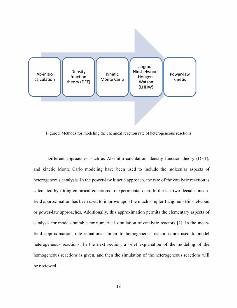
Figure 5 Methods for modeling the chemical reaction rate of heterogeneous reactions
Different approaches, such as Ab-initio calculation, density function theory (DFT),
and kinetic Monte Carlo modeling have been used to include the molecular aspects of
heterogeneous catalysis. In the power-law kinetic approach, the rate of the catalytic reaction is
calculated by fitting empirical equations to experimental data. In the last two decades mean-
field approximation has been used to improve upon the much simpler Langmuir-Hinshelwood
or power-law approaches. Additionally, this approximation permits the elementary aspects of
catalysis for models suitable for numerical simulation of catalytic reactors [2]. In the mean-
field approximation, rate equations similar to homogeneous reactions are used to model
heterogeneous reactions. In the next section, a brief explanation of the modeling of the
homogeneous reactions is given, and then the simulation of the heterogeneous reactions will
be reviewed.
Ab‐initio calculation
Density function
theory (DFT)
Kinetic Monte Carlo
Langmuir‐Hinshelwood‐
Hougen‐Watson (LHHW)
Power‐law kinetic
19
2.1.1 GAS-PHASE CHEMISTRY MODEL
Chemical reactions in the gas phase lead to source terms that are given as the mass
rate of creation and depletion of species by chemical reactions. The chemical source terms
are given as:
∑ ∏′
1, … , (16)
where is the molar mass of species , is the number of elementary gas-phase reactions,
(right side minus left side of reaction equation) and ′ (left side of reaction equation) are
stoichiometric coefficients, is the forward rate coefficient and is the concentration of
species . The temperature dependence of the rate coefficients is described by a modified
Arrhenius expression:
(17)
with as preexponential factor, as temperature coefficient, as activation energy, and
as the gas constant.
Because the chemical reaction systems are stiff, a direct calculation of the chemical
source terms , by equation (16), using the given temperature and concentrations, may easily
lead to divergence or oscillations of the iterative solution procedure. Therefore, a pseudo-time
integration is usually used to calculate the chemical source term.
Since the chemical source terms have to be calculated for each fluid cell and for each
iteration step, the total CPU time needed to achieve convergence increases dramatically if
detailed gas-phase chemistry is used.

20
2.1.2 SURFACE CHEMISTRY MODEL
The range of kinetic and transport processes that can take place at a reactive surface are
shown schematically in Figure 6. Heterogeneous reactions are fundamental in describing mass
and energy balances that form boundary conditions in reacting flow calculations.
There are three types of chemical species that describe the heterogeneous reactions:
- Species in the gas phase (gas species(g))
- Species residing at the interface of gas and solid (surface species(s))
- Species residing within the bulk solid (below the gas-surface interface) (bulk
species(b))
The surface species are those that are adsorbed on the top mono-atomic layer of the
catalytic particle while the bulk species are those found in the inner solid catalyst.
Each surface species occupies one or more surface sites. A site is considered to be a
location or position on the surface at which a species can reside. The total number of sites per
unit area is considered a property of the material surface, and is often assumed to remain
constant (site density).

21
Chemical kinetic rate expressions need to include the concentrations of the chemical
species. For gas-phase species the molar concentration (mol/m3) is written:
1, … , (18)
where the are the mass fractions, is the gas-phase mass density.
The composition of surface phases can be specified in terms of surface coverages . The
surface coverages in each phase are normalized:
∑ 1 (19)
The surface molar concentration of a species is then
Migration Migration
Bulk solid
Gas phase
Catalytic surface phase
Adsorption Adsorption
Reaction
Desorption
Figure 6 Schematic of the coupling between the gas and the surface due to transport and heterogeneous chemistry

22
Γ 1, … , (20)
where Γ is the surface site density (mol/m2) which describes the maximum number of species
that can adsorb on a unit surface area. The surface site densities are of the order of 10 mol/cm2
(approximately 10 adsorption sites per cm2) [29].
The surface chemistry is also modeled by elementary reactions similar to the gas-phase
reaction model. The chemistry source terms, , of gas-phase species due to
adsorption/desorption and surface species (adsorbed species) are given by:
∑ ∏′
1, … , (21)
where is the number of elementary surface reactions (including adsorption and desorption),
and is the number of species adsorbed. The heterogeneous flux on the surface is obtained by:
(22)
Since the catalyst is dispersed as small particles in the reactor support, the active catalyst
area is usually much greater than the geometric surface area. The ratio of these two values is
defined as:
/ (23)
To accounting for the pore diffusion within the catalyst coating layer, the effectiveness
factor, , is defined. / and are experimentally determined. Therefore, the heterogeneous
flux formula can be written as:

23
/ (24)
The temperature dependence of the rate coefficients in equation (21) is described by a
modified Arrhenius expression:
∏ Θμexp
Θ (25)
For some simple surface reaction mechanisms it is convenient to specify the surface
reaction rate constant in terms of a “sticking coefficient” (probability), rather than an actual
reaction rate. This approach is only allowed when there is exactly one gas-phase species reacting
with a surface:
Γτ (26)
where is the initial (uncovered surface) sticking coefficient, τ is sum of surface reactants’
stoichiometric coefficients.
Using equation (25), equation (21) can be rewritten as:
∑ ∏ Θμexp
Θ ∏′
1, … , (27)
From equation (20), δΘ
Γ and:
(28)
Note, equation (28) assumes that the total surface site density Γ is constant.
The equation above is used for a transient simulation. In a steady-state calculation,
surface species concentrations (or site fractions) remain constant with time [30], which gives:

24
0 1, … , (29)
At steady-state the surface species concentrations have to adjust themselves consistent
with the adjacent gas-phase species concentrations such that the condition 0is satisfied. In a
steady-state reacting flow simulation, the surface-species governing equations are taken to be
[20]:
0 1, … , 1
∑ 1 (30)
∑ ∏Γ
μ
exp Γ ∏′
0
1,… , 1 (31)
∑Γ
1 (32)
A normalization condition, equation (32), is used for one of the surface species to make
the system of equations well-posed.
The solution of equations (31) and (32) provides the surface coverages and the surface
molar concentrations. Once these have been obtained, the chemistry source terms can be
computed.
The system of equations generated by equations (31) and (32) is considered to be
extremely stiff. A system of ODEs is stiff if it forces the method to employ a discretization step
size excessively small with respect to the smoothness of the exact solution [31]. The Jacobian

25
matrix of a stiff system of ODEs has greatly differing magnitudes. Since most chemical kinetics
problems are stiff, many attemps were performed to find a stable and robust method for solving
them. For time-dependent problems, implicit methods are more stable than explicit methods. The
implicit time-integration methods are highly robust for time dependent problems but they
provide slow convergence to a steady state solution. Newton’s method provides a fast
(quadratically convergent property) and robust algorithms for solving the steady state problems,
but it only works when the initial guesses are within the domain of convergence. In practice, the
modern solution algorithms usually use a hybrid approach that combines the advantages of both
methods the implicit time-integration method and Newton’s method.
In the current work, a stiff solver using the Backward Differentiation Formulae (BDF)
method is developed. BDF methods with an unbounded region of absolute stability are widely
used for solving stiff ODEs. There are several possible ways of using a variable step size
including interpolated fixed-step BDF, fully variable-step BDF, and fixed-leading coefficient
BDF. The fixed-leading coefficient (FLC) BDF is used in the current work. The main advantages
of FLC BDF is that it does not suffer from the unstable behavior of the interpolated fixed-step
method and the Newton iteration matrix can be reused for more steps than in a fully variable-step
approach [32]. The Newton method is used for the solution of the resulting nonlinear system.
The linear algebraic system is solved using GMRES. For validation of the implementation, a stiff
solver software package is utilized. There are several software packages such as VODE [33] and
DASSL [34] that efficiently compute and produce high-accuracy solutions for stiff system of
ODEs. DASSL is based on fixed leading-coefficient BDF and can solve differential-algebraic
equations as well as stiff ODEs. VODE offers fixed leading-coefficient Adams and BDF
methods. The implicit formulae are solved via functional iteration or modified Newton,

26
depending on the option selected. Thus, this code has options for dealing with both stiff and non-
stiff problems. These solvers usually automatically switch between stiff and non-stiff methods to
achieve good performance. A C version of VODE, CVODE, is included in the SUNDIALS (
Suite of Nonlinear and Differential/Algebraic Equation Solvers) package.
To this end, the currently developed solver and CVODE are used for solving detailed
heterogeneous oxidation mechanism proposed by [35]. The surface reaction mechanism includes
24 heterogeneous reactions and 11 surface-adsorbed species. Figure 7 shows the runtime of
solving the stiff ODE systems for two solvers. As indicated in the figure, CVODE is much faster
than the solver developed herein. This may be due to greater optimization and faster algorithms.
Figure 7 Normalized runtimes for solving the stiff problem
Due to this improved performance, CVODE is chosen for solving the stiff equations. For
coupling the developed flow solver with CVODE, an interface based on Cantera [36] is used.

27
Cantera, written in C++, is a collection of object-oriented software tools for problems
involving chemical kinetics, thermodynamics, and transport processes. Cantera can be used in
Fortran or C++ reacting-flow simulation codes to evaluate properties and chemical source terms
that appear in the governing equations with fast and efficient numerical algorithms. Cantera
places no limits on the size of a reaction mechanism, or on the number of mechanisms [37].
The phase, interface definitions, and chemical reaction mechanisms are defined in a text
file (cti file). For example, a cti file written for the catalytic combustion of hydrogen on
palladium is shown in Appendix. 1. The cti file is converted into an XML-based format called
CTML using Cantera. There are several reasons for this conversion. XML is a widely-used
standard for data files, and it is designed to be relatively easy to parse. This makes it possible for
other applications to use Cantera CTML data files, without requiring the substantial chemical
knowledge that would be required to use cti files [36].
An interface is developed to link Cantera to the current flow solver. The structure of this
interface is illustrated in Figure 8. Based on the application, a Cantera input file is written which
includes the definition of the gas and surface phases and detailed chemical reactions. Input from
this file is used to create and allocate the Cantera gas, surface and interface objects at the
beginning of the simulation. During simulation, the flow solver provides the gas phase to
Cantera. This information includes the temperature, pressure, and mole fractions of the species.
Cantera specifies the required parameters, which is then provided to the CVODE solver. The
surface coverages and reaction rates are computed and communicated back to the flow
simulation solver to use as the chemical source terms.

28
Figure 8 Data exchange between the solver and Cantera through the interface
2.2. SENSITIVITY DERIVATIVES
In many engineering design applications, sensitivity analysis techniques are useful in
identifying the design parameters that have the most influence on the response quantities. This
information is helpful prior to an optimization study as it can be used to remove design
Open and read input file
Create the gas phase object
Create the surface phase object
Create the interface object (interface between surface-gas phases)
Flow solver
Gas temperature, pressure and mole fraction for the catalytic
wall boundary cell
T, P, Xk
Get the gas information
Set temperature, pressure and concentration for the gas and surface phases
Solve stiff equations using CVODE and compute surface coverages
Compute chemical reaction rates
Chemical reaction rates

29
parameters that do not strongly influence the responses. In addition, these techniques can
provide assessments as to the behavior of the response functions which can be invaluable in
algorithm selection for optimization, uncertainty quantification, and related methods. In a
post-optimization role, sensitivity information is useful in determining whether or not the
response functions are robust with respect to small changes in the optimum design point [38].
The sensitivities are obtained by computing gradients or derivatives of the solution with
respect to the set of design variables. There are many methods for computing and obtaining
sensitivities derivatives. A review of these methods may be found in [26]. Finite difference,
direct differentiation and adjoint methods have been widely used in the literature for this
purpose. The finite difference method is the simplest approach to compute sensitivity
derivatives. For a design variable and a cost function , the sensitivity derivatives are
obtained from a central difference as following:
∆ ∆
∆ (33)
which has a second-order truncation error and is subjected to subtractive cancellation. This
method is computationally expensive for a large number of design variables because two fully
converged nonlinear flow solutions are required for every design parameter.
The direct differentiation method is obtained by use of the chain rule. The residual
may be expressed in terms of explicit and implicit dependencies on the design variables as:
, , (34)
Applying the chain rule yields:

30
(35)
At convergence the residual and therefore the total differential are zero, that is
dR/dβ=0, and therefore the above may be solved for the sensitivity of the conserved variables
as:
(36)
In this linear system the Jacobian and sensitivity matrices, ∂R/∂Q and ∂R/∂β, are
evaluated using the CTSE method. Applying the chain rule to the cost function, assuming in
general that this function has both explicit and implicit dependencies on the design variables,
yields:
(37)
The linearization of the cost function can be evaluated analytically or by using the
CTSE method. Direct differentiation requires the solution to a linear system of equations for
each design variable and, thus provides an efficient method when the number of design
variables is relatively small.
In the adjoint method a constraint term, which is proportional to the residual through a
Lagrange multiplier [39], is added to the cost function:

31
, , , , , , (38)
where is the initial cost function, is an arbitrary vector of Lagrange multipliers and T is
the transpose operator. Linearizing the above with respect to the design variables yields:
(39)
Rearranging this equation to isolate the sensitivity of the conserved variables gives:
(40)
Since the Lagrange multipliers are arbitrary they are chosen to eliminate the first term
on the right hand side resulting in:
0 (41)
Once the Lagrange multipliers have been obtained by solving the above linear system,
sensitivity derivatives can be obtained from:
(42)
As can be seen, evaluation of the Lagrange multipliers only requires solution of one
linear system of equations for a given cost function. Therefore, the adjoint method is more
efficient than the direct differentiation approach for a large number of design variables.
32
CHAPTER 3
NUMERICAL SIMULATION OF CATALYTIC COMBUSTION IN STAGNATION FLOW
Since catalytic combustion includes a complex and coupled interaction of physics and
chemistry, researches usually use simple configurations to study and investigate them
numerically and experimentally. The stagnation flow field over a catalytically active foil is a
well-documented configuration and allows for the application of simple modeling and
measurement methods for analysis and study of heterogeneous combustion. Several researches
have studied the catalytic combustion of methane in a stagnation flow reactor. Deutschmann et
al. [40] investigated the heterogeneous oxidation of methane in a stagnation point flow
numerically and experimentally and obtained the ignition temperature 600˚C for the case. The
catalytic combustion of CH4, CO and H2 oxidation on platinum and palladium are studied
numerically by Deutschmann and et al. [41]. They presented the dependence of the ignition
temperature on the fuel/oxygen ratio. Dupont et al. [42] investigated numerically and
experimentally the dependencies of the methane conservation and CO selectivity on the surface
temperature for the catalytic combustion of methane on a platinum foil in a stagnation point flow
reactor. Most of research that has been done in the literature is related to the catalytic combustion
of methane. In this chapter, we first study methane oxidation on a platinum surface. After the
validation of numerical results with experimental data, the ignition temperature and the effects of
the surface temperature on the catalytic combustion are investigated. The catalytic partial
oxidation of iso-octane over a Rhodium (Rh) coated surface is considered as another test case.

33
Figure 9 shows the schematic of an axisymmetric stagnation-point flow. The stagnation
flow can be analyzed exactly using a similarity solution approach. In a similarity solution, the
number of independent variables is reduced by one using a coordinate transformation. For a
incompressible flow and ≪ 1, the exact flow equations using a similarity solution method
posses a solution with the following properties and assumptions [30]
- ( =Axial velocity)
-
-
-
- ( pressure-curvature term)
With these assumptions, the Navier-Stokes equations are reduced to a system of ODEs in
the axial coordinate z [30]:
2 0 (Mass continuity) (43)
(Radial momentum) (44)
(Species continuity) (45)
∑ ∑ (Thermal energy) (46)
∑ (47)

34
where is the diffusive flux, is the mixture specific heat, is dynamic viscosity, is thermal
conductivity, is molecular weight, is molar production rate of species and is the
enthalpy of species . The axial coordinate z is the independent variable and the axial velocity
( ), the scaled radial velocity ( ), the temperature ( ) and mass fractions ( ) are dependent
variables.
For the discretization of these equations, upwind differencing and central differencing are
used for convective and diffusive terms respectively. A MATLAB code is written to solve these
equations using a finite difference scheme. The CVODE computer program is used for the
solving the ODEs equations. The interface for COVE is created by a one-dimensional module of
Cantera. A hybrid Newton/time step algorithm suggested by [43] is used by Cantera to obtain the
steady state solution. The solver tries to find the steady-state solution by Newton’s method. If the
initial guesses lie within its domain of convergence, Newton’s method converges very fast.
However, it is hard to find a good starting vector for initializing these highly nonlinear problems.
In this case, a damping Newton’s method is used to improve the convergence rate, which is well
documented in [30]. Generally, two approaches, the line search method and the trust region
method are used for the damping process of Newton’s method. The line search parameter is
adjusted at each iteration to ensure that the next vector of solution is a better approximation to
the previous solution vector. This damping technique can improve the robustness but is not
effective in some problems. An alternative to a line search is the trust region method, in which an
estimate is maintained of the radius of a region in which the quadratic model is sufficiently
accurate for the computed Newton step to be reliable, and, thus, the next approximate solution is
constrained to lie within the trust region [44]. In the trust region method, both the direction and
the length of the Newton step can be modified when necessary. The damping parameters are

35
chosen to ensure that 1) mass fractions are between zero and unity 2) the next Newton step has a
smaller norm than the original undamped Newton step.
Figure 9 The schematic of stagnation-point flow
If the Newton iteration fails, the solver attempts to solve a pseudo-transient problem by
adding transient terms in each conservation equation. The solution algorithm used by Cantera is
illustrated in Figure 10.
The evaluation of the Jacobian matrix is the most computationally expensive operation
in this algorithm. For the fast convergence, the Jacobians are not computed at each iteration and
only calculated when the damped Newton algorithm failes [36].

36
Switch to pseudo-transient problem
Take a few time steps
Write the results
No
Yes
Start the steady-state problem using damping Newton’s method
Steady-state Newton succeeds
Start with the initial vector
Compute a Newton step
The solutions are inside the prescribed limits
Determine the scalar multiplier
Found the point inside the trust region where next Newton step
has a smaller norm than the original undamped Newton step
No
Yes
No
Yes
Figure 10 The solution algorithm for solving the ODE equations

37
3.1. METHANE OXIDATION ON A PLATINUM SURFACE
In this section, the catalytic combustion of methane on the platinum foil is investigated.
This case is chosen because there are many examples in the literature that performed numerically
and experimentally on this fproblem and it can be helpful for comparing our results with them
for validation of the numerical data. As indicated in Figure 11, a lean mixture of methane-air
with a uniform velocity distribution is injected at the distance 10 cm above the reactive surface.
The flow field variables including density, velocity, species mole fractions and temperature are
independent of radius and depend only on the distance from the surface. The boundary
conditions are illustrated in Figure 11. Since there is no net mass exchange between the gas and
surface, the Stefan velocity (ust) is zero.
The simulations are performed with the detailed heterogeneous oxidation mechanism
proposed by [41]. The surface reaction mechanism is shown in Table 2. It consists of 24
heterogeneous reactions, including 11 surface-adsorbed species. Since the ODE system of
equations is stiff, a proper procedure should be used to make sure the solution is well converged.
For this case, the problem is solved first for a hydrogen-oxygen case to provide a good initial
estimate for methane-air test case. In addition, the solver is first run without the heterogonous
reaction rate and then the chemistry source term is added gradually. The solution is started with
an initial grid with 10 nodes and refined if needed during the solution. The simulations showed
that a grid with 40 nodes provides a robust and good solution.

38
For validation of the numerical results, the experimental data provided by reference [42]
is used. Figure 12 shows the comparison between the obtained numerical results with
experimental data. The fuel conversion index (FCI) is defined as the ratio of fuel mass consumed
to inlet mass flux of fuel [42]. As seen in Figure 12, good agreement is obtained.
The velocity and temperature profiles are indicated in Figure 13. The axial velocity is
changed from the inlet value to zero on the surface. The radial velocity is increased to its
maximum value near the surface and then sharply decreased to zero on the surface.
u= ust V =v/r=0 T=T_surface
ρYk(Vdiff+ust)=MWkωk Reactive surface
u=8 cm/s
V =v/r= 0
T=300 K
10 cm
Figure 11 Geometry and boundary conditions for catalytic combustion of methane on the platinum surface

39
Table 2 Reaction mechanism for methane combustion on a Pt surface [6]
Catalytic ignition refers to phenomena where sufficient energy is released from a
catalytic reaction to maintain further reaction without additional external heating [45].
Deutschmann et al. [40] experimentally obtained an ignition point around 873 K for the catalytic
combustion of methane on the platinum foil. The present work investigates the behavior and
changes of the heterogeneous mechanism at different temperatures around the ignition point. The
effect of the surface temperature on the profile of methane mole fraction is shown in Figure 14.

40
At the low temperature 700 K, the methane concentration is almost constant and no methane is
consumed. Increasing the surface temperature causes the methane consumption to be enhanced
and at a temperature of about 1400 K, all of methane is depleted.
Figure 12 The comparison between the obtained numerical results with experimental data reported by [42]

41
Figure 13 Velocity and temperature profiles for the surface temperature 800 K
Figure 14 Effect of the surface temperature on CH4 concentration

42
Figure 15 shows the variation of the surface phase mass fraction with temperature. The
site density is 2.7063e-9 and initial converages of the surface is H(S) =0.5 and Pt(S) =5. At the
lower temperature, the platinum surface is mainly covered by oxygen. The oxygen coverage is
decreased with increasing temperature, especially after the ignition point and O(S) is consumed
by the OH(S) and CO(S) formation reactions.
As seen in Figure 16, the main products of this heterogeneous mechanism are CO2 and
H2O. The CH4 and oxygen are consumed near the reactive surface and produce CO2 and H2O.
Figure 15 Surface site fraction for the different surface temperature

43
Figure 16 Gas phase species concentrations for the surface temperature 1200 K

44
3.2. CATALYTIC PARTIAL OXIDATION OF ISO-OCTANE OVER RHODIUM (RH)
COATED SURFACE
The catalytic combustion of iso-octane over a rhodium/alumina coated honeycomb
monolith is investigated as another test case. The initial and boundary conditions are given in
Figure 17.
The heterogeneous combustion of iso-octane on a rhodium-based catalyst is modeled by a
detailed surface reaction mechanism proposed by Hartmann et. al [46]. Table 3 shows the details
u= ust V =v/r=0 T=T_surface
ρYk(Vdiff+ust)=MWkωk Rh-coated surface
u=1 cm/s
V =v/r= 0
T=300 K
10 cm
Figure 17 Geometry and boundary conditions for catalytic combustion of iso-octane over the Rhodium surface

45
of the chemistry model. The surface chemistry mechanism includes 17 surface species and 58
surface reactions.

46
Table 3 Reaction mechanism for iso-octane combustion on a Rh surface [12]
47
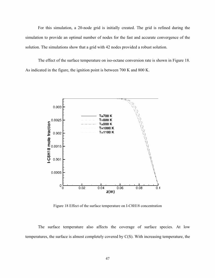
For this simulation, a 20-node grid is initially created. The grid is refined during the
simulation to provide an optimal number of nodes for the fast and accurate convergence of the
solution. The simulations show that a grid with 42 nodes provided a robust solution.
The effect of the surface temperature on iso-octane conversion rate is shown in Figure 18.
As indicated in the figure, the ignition point is between 700 K and 800 K.
Figure 18 Effect of the surface temperature on I-C8H18 concentration
The surface temperature also affects the coverage of surface species. At low
temperatures, the surface is almost completely covered by C(S). With increasing temperature, the

48
value of C(S) is decreased and O(S) and CO(S) are the dominant surface species as shown in
Figure 19.
Figure 19 Surface coverages for the different surface temperature
Figure 20 shows the gas phase concentration along the injection to surface at the
temperature 1100 K. The iso-octane is oxided and combusted almost completely on the surface
and products are mainly H2O, CO and CO2.

49
Figure 20 Gas phase species concentrations for the surface temperature 1100 K

50
CHAPTER 4
CATALYTIC PARTIAL OXIDATION OF METHANE
To organize and present the research in this chapter, the computational results are divided
into a number of sections. For the catalytic partial oxidation of methane, these sections
specifically address the parallel performance of the developed methodology, validation with
experimental data, parametric study of design parameters, sensitivity analysis, and design
optimization.
4.1. PARALLEL PERFORMANCE
The parallel performance of the currently developed methodology is assessed using the
simulation for the catalytic partial oxidation of methane. The details concerning this simulation
are presented in the following section, and are not presently required to assess algorithmic
performance. The developed methodology utilizes standard Message Passing Interface (MPI)
libraries, and the scalable performance is examined over an increasing range of processors. The
simulations are performed on an in-house SimCenter cluster. This cluster has 325 dual-processor
dual-core machines (1300 cores total), E1200 Gigabit Ethernet switches, and a cluster
performance of 7.7 terraflops (TF).
Considering 10 Newton iterations, the execution times for 1, 2, 4, 8, 16, 32, 64 and 128
processors are shown in Figure 21. As illustrated in the figure, run time is decreased with
increased number of processors. However, for evaluating the parallel efficiency, it more useful

51
to ascertain how much performance gain is achieved by parallelizing a given problem over a
serial implementation. The speedup is a measure that captures the relative benefit of solving a
problem in parallel. Speedup is defined as the ratio of the time taken to solve a problem on a
single processor to the time required to solve the same problem on a parallel system [48]:
(48)
Figure 21 The total run times for the different number processors
The speedup for the current case is presented in Figure 22. As indicated, the speedup is
decreasing with increasing the number of the processors. The computing speedup is close to the
ideal speedup for the number of processors less than 10. Increasing number of processors for a
fixed size problem, the communication overhead is increased, and which lead to decreasing

52
speedup. This result is typical in that for a given discretization, the amount of computational
work is fixed, and as the number of processors is increased the communication costs become
more significant. For larger problem sizes, the theoretical speedup is achieved for a larger
number of processors.
Figure 22 Parallel performance using Speedup

53
4.2. VALIDATION FOR THE CATALYTIC PARTIAL OXIDATION OF METHANE
In this section, the catalytic partial oxidation of methane over Rh/Al2O3 coated
honeycombs is numerically investigated. Honeycomb-structured reactors are widely used in
many engineering applications such as fuel reformers, catalytic converters, and gas turbine
combustors. The experimental study conducted by Hettel et al. [14] is selected for validation
purposes. In the experimental study the reactor is a 2 cm diameter cylinder, with 260 channels,
and a channel density of 600 cpsi (channels per square inch). The initial and boundary conditions
are summarized in Table 4. The simulations are performed with the detailed heterogeneous
oxidation mechanism proposed by Deutschmann et al. [35], and include 38 heterogeneous
reactions and 20 surface-adsorbed species. The site density is assumed to be 2.79
10 mol/cm , and the kinetic data of the surface-reaction mechanisms are taken from the
literature. Eight gas-phase species (CH4, CO2, H2O, N2, O2, CO, OH and H2) are considered for
the simulation, with the surface chemistry modeled using the mean-field approximation. Since it
has no significant effect on the flow field for this test case and operating conditions, the
homogenous combustion in the gas phase is ignored in this study [47]. The computational grid is
comprised of 122,208 tetrahedral cells, and the parallel simulation performed with 64 processors.
Figure 23 depicts the surface grid for one channel of the monolith. The grid is refined in the
regions near the catalytic wall to accurately resolve the boundary layer. The “inflow” boundary
condition is used at the channel inlet, and a fully developed boundary condition is considered for
the outlet. The no-slip boundary condition with a catalytic reaction source term is applied at the
channel walls. The temperature of the catalytic wall is assumed to be constant along the channel.
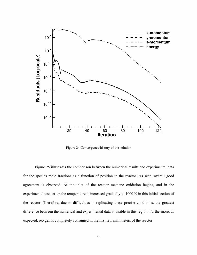
The nonlinear system of equations obtained from the discretization is solved using Newton’s
method, and the convergence history of the solution is shown in Figure 24.

54
Table 4 Initial conditions for catalytic partial oxidation of methane
Gas inlet velocity 0.329 m/s
Gas inlet temperature 1000 K
Wall temperature 1000 K
Gas inlet compositions (mole fraction) x 0.133, x 0.067,
x 0.8
Working pressure 1 atm
Channel width 1 mm
Channel length 10 mm
Figure 23 Grid generated for the channel of reactor
55
Figure 24 Convergence history of the solution
Figure 25 illustrates the comparison between the numerical results and experimental data
for the species mole fractions as a function of position in the reactor. As seen, overall good
agreement is observed. At the inlet of the reactor methane oxidation begins, and in the
experimental test set-up the temperature is increased gradually to 1000 K in this initial section of
the reactor. Therefore, due to difficulties in replicating these precise conditions, the greatest
difference between the numerical and experimental data is visible in this region. Furthermore, as
expected, oxygen is completely consumed in the first few millimeters of the reactor.

56
Figure 25 Comparison between the numerical results and experimental data for the partial oxidation of
methane
Rhodium and platinum are considered good catalysts in terms of stability and yields.
They are widely used for partial oxidation and catalytic combustion of methane in fuel
reformers, catalytic burners and catalytic gas turbines. To better understand the performance of a
methane reformer with these two catalysts, numerical simulations are performed. The detailed
heterogeneous oxidation mechanisms developed by Deutschmann et al. [35] (24 heterogeneous
reactions and 11 surface-adsorbed species) and Deutschmann et al. [41] (38 heterogeneous
reactions and 20 surface-adsorbed species) are used to model surface chemistry for rhodium and
platinum, respectively. The temperature of the catalyst wall is fixed to 1070 K. The inlet velocity
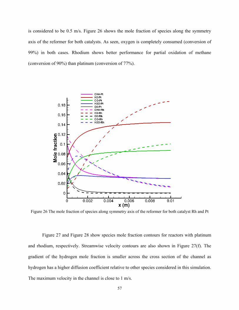
57
is considered to be 0.5 m/s. Figure 26 shows the mole fraction of species along the symmetry
axis of the reformer for both catalysts. As seen, oxygen is completely consumed (conversion of
99%) in both cases. Rhodium shows better performance for partial oxidation of methane
(conversion of 90%) than platinum (conversion of 77%).
Figure 26 The mole fraction of species along symmetry axis of the reformer for both catalyst Rh and Pt
Figure 27 and Figure 28 show species mole fraction contours for reactors with platinum
and rhodium, respectively. Streamwise velocity contours are also shown in Figure 27(f). The
gradient of the hydrogen mole fraction is smaller across the cross section of the channel as
hydrogen has a higher diffusion coefficient relative to other species considered in this simulation.
The maximum velocity in the channel is close to 1 m/s.

58
Figure 27 Contour plots for the reactor with Platinum catalyst a) CH4 mole fraction b) H2 mole fraction c)
O2 mole fraction d) H2O mole fraction e) CO mole fraction f) x-velocity

59
Figure 28 Contour plots for the reactor with Rhodium catalyst a) CH4 mole fraction b) H2 mole fraction
c) O2 mole fraction d) H2O mole fraction e) CO mole fraction

60
4.3. PARAMETER STUDY
In this section, the effect of the different design parameters on the fuel reformer
performance is investigated. These design parameters can be related to the shape/size of the
reformer as well as the operating conditions and catalyst material. In this work the inlet
methane/oxygen ratio, inlet velocity, and catalytic wall temperature are considered as variables
for parametric study. Note that by using the inlet velocity as one of the parameters, the effect of
different Reynolds numbers on reformer performance is also studied indirectly.
The baseline conditions for this study are shown in Table 5. Figure 29 shows the
comparison of the mole fraction of species along the symmetry axis of the reformer with two
different inlet velocities of 0.5 and 2 m/s. The conversion of methane is predicted to decrease
with increasing inlet velocity. The rate of oxygen consumption along the reactor is also
decreased and therefore the peak of H2O concentration is shifted towards the middle of the
channel for the higher inlet velocity. Mole fraction contours of the different species for the
reactor with inlet velocity of 2 m/s are illustrated in Figure 30.

61
Table 5 Baseline conditions for catalytic combustion of methane
Gas inlet velocity 0.5 m/s
Gas inlet temperature 1070 K
Wall temperature 1070 K
Gas inlet compositions(mole fraction) x 0.133, x 0.067, x 0.8
Working pressure 1 atm
Channel width 1 mm
Channel length 10 mm
Catalyst Rh
Figure 29 The comparison of the mole fraction of species along symmetry axis of the reformer with the different inlet velocities 0.5 and 2 m/s

62
a)
b)
c)
d)
e)
Figure 30 The mole fraction contour for the reactor with the inlet velocity 2 m/s

63
The influence of the catalytic wall temperature on species conversion rates is shown in
Figure 31. The numerical results predict that the conversion of methane increases from 90% at
1070 K to 96% at 1170 K. Additionally, hydrogen production is increased by approximately
10% at the higher temperature.
Figure 31 The comparison of the mole fraction of species along symmetry axis of the reformer for the
different catalytic wall temperature

64
The inlet methane-oxygen ratio represents another important design parameter. To
investigate the influence of this ratio, two different simulations were performed. These consisted
of methane-oxygen ratios of 1 ( 0.1 and 0.1) and 1/3 ( 0.05and 0.15).
The numerical results are shown in Figure 32, which compares the aforementioned cases with a
baseline methane-oxygen ratio of approximately 2 0.133 and 0.067 . Figure 32
demonstrates the influence of the methane-oxygen ratio on reformer performance. As seen, the
size of the active methane conversion region increases with higher methane-oxygen ratios at the
inlet. The hydrogen production reaches the highest level for the most-fuel-rich mixture.
Hydrogen production for the mixture ratio of 1/3 is minimal and CO, CO2 and H2O are the main
products, as can be seen from the mole fraction contours illustrated in Figure 33.
Figure 32 The influence of the variation of methane/oxygen ratio on the reformer performance

65
a)
b)
c)
d)
e)
f)
Figure 33 The mole fraction contour for the reformer with the methane/oxygen ratio 1/3

66
Catalyst loading is an import factor in the design and optimization of catalytic reactors.
The heterogeneous flux with catalyst loading effects has been previously given in equation (24).
For considering the effect of catalyst loading, two parameters F / (ratio of catalytic surface
area to geometric surface area) and η (effectiveness factor) are considered. As shown in Figure
34, the methane conversion increases for high catalyst loading. The methane conversion
increases from 57% at F / η 0.5 to 98% at F / η 2, and the hydrogen production at
F / η 2 increases about 7% relative to the baseline case. Additionally, oxygen is almost
completely consumed by surface reactions in the first millimeter of the reactor length for all
three cases. For F / η 0.5 the contours of the concentrations of species along the length of
the reactor are shown in Figure 35 to illustrate the variations within the channel.
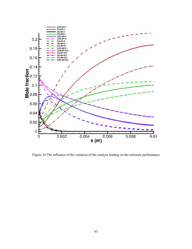
67
Figure 34 The influence of the variation of the catalyst loading on the reformer performance

68
a)
b)
c)
d)
e)
f)
Figure 35 The mole fraction contour for the reformer with F / η 0.5
69
4.4. SENSITIVITY ANALYSIS
For the parametric studies, the dependencies of the reformer performance on design
variables were obtained by comparing baseline solutions to those with variations. An alternative
approach to assessing these effects is through the use of sensitivity analysis. In this method, the
sensitivities are obtained by computing gradients or derivatives of the solution with respect to the
set of design variables. These sensitivity analysis methods, having widely varying
implementation costs, provide a precise sensitivity measure at roughly the same cost as a
function evaluation [26]. As previously discussed, there are several methods for computing
sensitivity derivatives.
The typical use of sensitivity analysis is for computational design whereby the cost
function is to be either minimized or maximized. To improve the cost function, gradient-based
optimization algorithms require information on how the cost function changes with respect to the
design variables; that is, dI dβ. Furthermore, sensitivity derivatives may be used to identify the
variables that have the most significant impact on design performance. Design variables of the
inlet velocity, methane density, oxygen density, catalytic wall temperature, and catalytic area
ratio are considered for sensitivity analysis in this study. The mean value of H2 concentration at
the outlet boundary is considered as the cost function. For verification purposes, sensitivity
derivatives obtained using the adjoint and direct differentiation approaches are compared with
those computed using a central finite-difference method. For the central finite-difference method,
a perturbation value of 1 10 is used for the simulation. The baseline conditions for this study
have been previously given in Table 5. Sensitivity derivative results are presented in Table 6. As
illustrated in Table 6, the sensitivity derivatives obtained by the direct differentiation and adjoint
methods show good agreement, and match up to nine digits. Additionally, it may be observed

70
that methane concentration, followed by oxygen concentration, plays the most significant roles in
the mean value of H2 concentration. Differences are observed in comparisons with the central
finite-difference method. These discrepancies may be attributable to the highly nonlinear
response of the cost function to the design variables and due to subtractive cancellation errors in
the finite-difference method. To ascertain a better understanding on the sources of errors, a more
detailed step-size study for the finite-difference method is warranted.
Table 6 The sensitivity derivatives for the different design variables
DV finite difference direct differentiation adjoint
Inlet velocity -0.00571674320 -0.00580817201 -0.00584081720
Inlet methane
concentration 0.10364058231 0.10718769820 0.10718769812
Inlet oxygen
concentration -0.080342139543 -0.079660588349 -0.079660588319
Catalytic wall
temperature 0.00116746547 0.00105843297 0.00105843127
Catalytic area
ratio 0.00104274151 0.00113610487 0.00113610454
4.5. OPTIMIZATION
In gradient-based optimization algorithms, sensitivity derivatives are utilized in
determining a search direction that will maximize or minimize the cost function. One potential
drawback to these methods is the added complexity and computational costs associated with
evaluating these gradients. However, sensitivity analysis requires solutions to linearized systems
of equations, whereas finite-difference methods necessitate the solution to nonlinear systems for
each design variable perturbation. Furthermore, as noted previously, the discrete adjoint method

71
eliminates the dependence of the sensitivity of the cost function with respect to the state-vector
and, therefore, represents an efficient means to evaluate sensitivity derivatives for large number
of design parameters. Since the number of design variables is small in this case, there is no
significant advantage of using the adjoint method relative to the direct differentiation. Thus, the
direct differentiation method is utilized.
Optimization is the minimization or maximization of a function subjected to constrains
on its variables. The optimization problem can be defined as
min ∈
Subject to: 0 ∈
(49)
where is the objective or cost function, is the vector of inequality constraints,
and and the lower and upper side-constraints on the design variable, respectively.
Numerous algorithms have been developed for solving this standard optimization problem and,
moreover, are available in software packages.
In the current research, the DAKOTA toolkit is used. DAKOTA (Design Analysis Kit for
Optimization and Terascale Applications) was developed at Sandia National Laboratories [38].
DAKOTA’s optimization capabilities include a wide variety of gradient-based and nongradient-
based optimization methods. It includes many external optimization libraries such as the OPT++
library [49], CONMIN and DOT libraries [50], and an interface to link with third-party routines
that provide the function evaluations and sensitivity information.
An interface is created to link the flow solver to DAKOTA. Figure 36 shows the
workflow involving the flow solver and DAKOTA. The output file from DAKOTA containing

72
new values for the solver is “params.in”. This file is created by DAKOTA during each design
cycle.
Figure 36 The data interchange and interface between the flow solver and DAKOTA
Initially, to demonstrate the numerical optimization procedure, three design parameters
including inlet velocity, inlet methane concentration, and catalytic wall temperature are studied.
For this optimization, the mean value of CH4 concentration at the outlet boundary is considered
as the cost function, and the initial conditions on the design parameters of inlet velocity, inlet
methane concentration, and catalytic wall temperature are 0.7 m/s, 0.05, and 1000 K,
respectively. The initial concentration for oxygen and nitrogen are 0.15 and 0.8, respectively. All
other conditions are the same as found in Table 5. Note that since the values of the design

73
variables have different orders of magnitude, scaled values are used within the optimization for
methane concentration and catalytic wall temperature. Additionally, side-constraints are imposed
on these design variables and are listed in Table 7.
Table 7 Initial values and constrained bounds for the design variables
inlet velocity methane concentration at inlet catalytic wall temperature
Lower bound 0.3 0.3 0.8
Upper bound 1.5 1.3 1.2
Initial values 0.7 0.5 1.0
The optimization is performed using two gradient-based algorithms: the Fletcher-Reeves
conjugate gradient (frcg) method (from DAKOTA’s CONMIN library) and a quasi-Newton
method (from DAKOTA’s OPT++ library). Both methods achieve the same local optimal point
of 0.3 m/s, 0.0825, and 1200 K for inlet velocity, methane concentration, and catalytic wall
temperature, respectively. Note that in this case, the lower side-constraint for inlet velocity and
the upper side-constraint for catalytic wall temperature are active. For this particular
optimization, as seen in Table 8, the quasi-Newton algorithm requires significantly more gradient
calculations and design cycles as compared to the Fletcher-Reeves conjugate gradient method.
Figure 37 shows a comparison of methane concentration along the centerline of the reactor using
baseline and optimized conditions.

74
Table 8 the number of solver and gradients calls for the optimization algorithms
Method function evaluation gradient calculations
Fletcher-Reeves conjugate
gradient method
17 7
quasi-Newton algorithm 17 15
Figure 37 The comparison between the optimized conditions for methane concentration along the reactor
While the previous case optimized the methane conversion, the main goal of reformer
design is to maximize the hydrogen production. In some cases, although methane is almost
compeletly consumed for the given conditions, the main products of the chemistry are species
other than hydrogen. For this reason, a cost function representing the hydrogen concentration at
the outlet boundary may be defined as

75
1 ∬
0.09 (50)
Based on the previous optimization results using high-fidelity analysis, the Fletcher-
Reeves conjugate gradient method is selected for this case. Again, the design variables of inlet
velocity, wall temperature and inlet methane concentration are used, and the initial conditions on
these design parameters are 0.7 m/s, 0.082, and 1000 K, respectively. The initial concentration
for oxygen and nitrogen are 0.118 and 0.8, respectively. For this optimization, 20 objective
function evaluations and 5 gradient calculations were required to obtain the local minimum point
of 0.545 m/s, 0.13, and 1200 K. A comparison of hydrogen concentration along the centerline of
the reactor using baseline and optimized conditions is shown in Figure 38.
Figure 38 The comparison between the base condition and the optimized condition for hydrogen concentration along the centerline of the reactor

76
CHAPTER 5
NUMERICAL SIMULATION A HONEYCOMB-STRUCTURED CATALYTIC REFORMING REACTOR
The chemical and thermal phenomena within the full reactor are computationally
investigated in this section. Two monolithic reactors were simulated.
The first test case is a cylindrical monolith with diameter 1.84 cm and length 10 cm as
shown in Figure 39. The channels have a square cross-section of dimension 1.6 mm * 1.6 mm
[6]. Since the geometry is symmetric, only a quarter of the reactor is simulated. A grid with
1,261,820 prism cells is generated by Pointwise [51] as indicated in Figure 40. Figure 41 shows
the boundary conditions used to model this problem. The reactor performance is investigated
with two different inflow conditions. Table 9 shows input mole fractions for two test conditions.
The simulations are performed on the in-house SimCenter cluster.

77
Figure 39 The cylindrical monolithic reactor with square cross-section channels
Figure 40 The generated grid for the monolithic reactor

78
Figure 41 The boundary conditions for the monolithic reactor and mesh cross-section
Table 9 Initial conditions for fuel reforming reactor
Test conditions 1 Test conditions 2Gas inlet compositions(mole fraction)
0.0449 0.133
0.1934 0.067
0.7545 0.8
0.0072 0.0 Gas inlet velocity 0.329 m/s 0.329 m/s Gas inlet temperature 975 K 975 K Reactor temperature 1000 K 1100 K Working pressure 1 atm 1 atm
The governing equations are similar to what were described in Chapter 2, but one
additional equation for the solid phase is added. Therefore, the system of equations is:
. (51)

79
where
⋮
∑
(52)
⋮
0
⋮
0
⋮
0
(53)
⋮
0
⋮
0
⋮
(54)
⋮
00000
(55)

80
Since eight gas-phase species (CH4, CO2, H2O, N2, O2, CO, OH and H2) are considered in
the simulation, the number of equations is 13 (8 mass conservations, 3 momentum conservations,
1 energy conservation for fluid phase and 1 energy conservation for the solid phase.
The contours of the velocity and temperature for test condition 1 are shown in Figure 42.
Since the reactor wall is isothermal, the temperature within the reactor in steady state condition is
reaches 1000 K. In the reactor channels, fully developed temperature profiles are recognized.
The maximum velocity within the reactor channels is 1.1 m/s.
a)
b)
Figure 42 Contours of a) Temperature b) Velocity for the reactor at test conditions 1
In the test condition 1, contours of mole fraction within the reactor are indicated in Figure
43. With the inlet boundary condition in this case, products are mainly H2O and CO. Since the
inlet concentration of methane is small, no significant oxidation is shown in the process and
oxygen is not completely consumed. The conversion of methane in this case is about 85%.

81
a)
b)
c)
d)
e)
f)
Figure 43 Contour plots for species mole fractions for test condition 1 a) CH4 b) CO2 c) CO d) H2 e) H2O f) O2

82
The reactor is performed as a methane fuel reformer in the test condition 2. At the test
condition 2, the temperature of the reactor is fixed to 1100 K and inflow concentrations are
changed. Temperature and velocity contours are shown in Figure 44. The maximum velocity in
this case is increased compared with the previous one because the reactor temperature is
increased. As indicated in Figure 45, concentrations of the species are totally different compared
with the previous case. Hydrogen is the main product of this process. The oxygen is completely
consumed and the conversion of the methane is about 91%. As shown in both test cases, the
gradient of the hydrogen mole fraction is smaller across the cross section of the channel because
hydrogen has a higher diffusion coefficient relative to other species considered in this simulation.
a)
b)
Figure 44 Contours of a) Velocity b) Temperature for the reactor at test conditions 2

83
a)
b)
c)
d)
e)
f)
Figure 45 Contour plots for species mole fractions at test conditions 2 a) CH4 b) CO2 c) CO d) H2 e) H2O f) O2

84
In the second test case, the reactor is a rhodium-coated monolithic honeycomb with a 2
cm diameter cylinder and a channel density of 600 cpsi (channels per square inch). A value of 2
W/(mK) was used for the thermal conductivity of the solid. The structure of the reactor is
illustrated in Figure 46. For simulations, a quarter of the reactor is considered because of the
symmetry properties. Figure 47 and Figure 48 indicate the mesh and the boundary conditions
used in the numerical analysis, respectively. A number of 3,308,100 prism cells (9,924,300) with
triangular base are generated with Pointwise software [51] for analyzing of the catalytic
combustion within the reactor.
Figure 46 The structure of the reactor
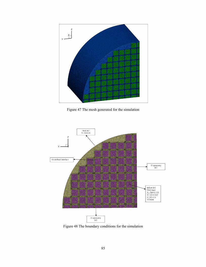
85
Figure 47 The mesh generated for the simulation
Figure 48 The boundary conditions for the simulation
86
Figure 49 shows the contour of species concentration within the reactor. As shown in the
figure, variation of the gas mass concentrations along the reactor are almost the same for all the
inner channels. The only difference is in the channels near the external boundary of the reactor.
The temperature distribution within the reactor has a significant effect on the mass concentration
of species and eventually the reactor performance. Because the temperature distribution in the
regions close to the external boundary of the reactor is different from other regions, a different
flow pattern is seen within the reactor. The difference for the species of H2 and CO2 is more
visible, and the O2 mass fraction is less sensitive to the temperature distribution within the
reactor.

87
a)
b)
c)
d)
Figure 49 Contour plots for the reactor a) O2 mole fraction b) CH4 mole fraction c) H2 mole fraction d) CO2 mole fraction e) Temperature
5.1. SENSITIVITY ANALYSIS OF THE FULL REACTOR
The following two cost functions are considered for sensitivity analysis:
Case-1: the mean value of the CH4 concentration at the outlet boundary.
Case-2: the mean value of the H2 concentration at the outlet boundary.

88
The operating conditions are the same as described in test condition 2 of Table 9.
Improving the performance of the fuel reforming is the ultimate goal of the reactor design: the
first cost function is minimizing of CH4 concentration, and the second cost function is the
maximizing of H2 concentration. Sensitivity derivatives of the cost functions representing the
reactor performance with respect to various design parameters can be extremely useful in the
design cycle.
Four design parameters are included to compute sensitivity derivatives of the
aforementioned objective functions. The design parameters are the inlet velocity, the inlet
methane concentration, the inlet oxygen concentration and thermal conductivity of monolith.
Table 10 shows the sensitivity derivatives of both cost functions obtained using the
discrete adjoint method for the full reactor.
Table 10 Sensitivity derivatives of both cost functions obtained using the discrete adjoint method for the full reactor
DV Cost-1 Cost-2
Inlet velocity 5.6876980509e-3 -1.7594093681e-3 Inlet methane density 1.1162738317e-1 1.8562329355e-1 Inlet oxygen density -3.5172116328e-2 -8.3257422654e-2 Thermal conductivity of monolith -1.1102201864e-4 2.4238135909e-5

89
CHAPTER 6
CONCLUSION
6.1. SUMMARY
The complex interaction of chemical and physical processes inside the methane
reforming reactor is numerically studied with an implicit, unstructured finite volume based
multi-species Navier-Stokes solver. The surface chemistry, heterogeneous combustion and
coverages are computed and solved by coupling the high-fidelity simulation with Cantera.
Coupling with the Cantera package enabled solving the stiff system of equations encountered
while modeling the surface chemistry. The governing equations for the fluid and solid phases
(the reactor’s body) are solved simultaneously. For validation, numerical results are compared
with experimental data and good agreement is observed for the catalytic partial oxidation. To
assess the effect of various parameters on reactor efficiency, a parametric study was performed.
This study indicated that the conversion of methane decreases with increasing inlet velocity and,
therefore, Reynolds number. Moreover, the methane and hydrogen production increases with
increasing catalytic wall temperature; methane conversion decreases with increasing
methane/oxygen ratio, and hydrogen production is higher at richer mixtures. Sensitivity analysis
was additionally used to assess the effect of design parameters on reactor performance.
Verification of these sensitivity derivatives was performed using finite-difference, direct
differentiation, and adjoint formulations. From sensitivity analysis it was observed that the
methane concentration, followed by oxygen concentration, play the most significant roles in the

90
mean value of H2 concentration. Finally, utilizing the sensitivity analysis capability,
computational design was performed with a gradient-based optimization algorithm. Considering
the inlet velocity, wall temperature and inlet methane concentration as design variables, two
optimization cases were performed. The first optimization selected the mean value of CH4
concentration at the outlet boundary as the objective function, and compared the numerical
performance of Fletcher-Reeves conjugate gradient and quasi-Newton algorithms. The second
optimization case selected hydrogen concentration at the outlet boundary as the objective
function, and demonstrated significant reactor improvement over the baseline design. The results
obtained from the optimization process show that numerical optimization can be successfully
used to improve the performance of the reactor with less computational cost than conventional
methods.
6.2. RECOMMENDATIONS FOR FUTURE WORK
The catalytic reactors are mainly used in fuel reforming and can be worked in three
different reforming modes of steam reforming (SR), partial oxidation (POX) and autothermal
reforming (ATR). Catalytic combustion is also used in a wide variety of applications, mainly
driven by environmental concerns like automotive catalytic converters, gas turbine and selective
catalytic reactor for reduction of pollutants and production of low temperature heat.
Catalytic reactors are generally characterized by the complex interaction of various
physical and chemical processes. Because of the complexity and coupled interaction of the mass
and heat transfer, design and optimization of catalytic reactors is difficult and expensive.
Computational fluid dynamics (CFD) can be used as an appropriate tool for the understanding
the interaction of physics and chemistry in the reactor and support reactor design and

91
engineering. CFD also can be used for the supporting of the experimental tests. It also can be a
time-efficient and inexpensive alternative to trial-and-error experimental investigations.
Some extensions may be:
Model the heterogeneous reaction rates with some fundamental methods like Ab-initio
calculation, Density function theory (DFT) and Kinetic Monte Carlo.
Extend the numerical simulations to other engineering and industrial applications like
automotive catalytic converters and stationary gas turbines for reducing pollutants.
Consider the homogenous combustion in the simulations and study the effects on the
distribution of gas species within the reactor
Develop the numerical model to investigate the behavior of the catalytic combustion of
fuel reformers with more complex features and with heavy fuels like Diesel.
Increase the speed up of the numerical procedure using GPU-accelerated computing in
solving the stiff system of equations of the surface chemistry.

92
REFERENCES
[1] R. E. Hayes and S. T. Kolaczkowski, Introduction to Catalytic Combustion, Gordon and Breach Science Publishers, 1997.
[2] O. Deutschmann, Modeling and Simulation of Heterogeneous Catalytic Reactions, Wiley-VCH, 2012.
[3] H. D. Minh, Numerical Methods for Simulation and Optimization of Chemically Reacting Flows in Catalytic Monoliths, PhD Thesis, University of Heidelberg, 2005.
[4] M. Hettel, C. Diehm, B. Torkashvand and O. Deutschmann, "Critical Evaluation of In-situ Probe Techniques for Catalytic Honeycomb Monoliths," Catalysis Today, vol. 216, 2013.
[5] A. Kumar, Physical Models and Computational Algorithms for Simulation of Catalytic Monolithic Reactors, PhD Thesis, Ohio State University, 2009.
[6] L. L. Raja, R. J. Kee, O. Deutschmann, J. Warnatz and L. D. Schmidt, "A critical evaluation of Navier–Stokes, boundary-layer, and plug-flow models of the flow and chemistry in a catalytic-combustion monolith," Catalysis Today, vol. 59, no. 1-2, pp. 47-60, 2000.
[7] A. E. Cerkanowicz, R. B. Cole and J. G. Stevens, "Catalytic Combustion Modeling; Comparisons With Experimental Data," ASME. J. Eng. Power, vol. 99, no. 4, pp. 593-600, 1997.
[8] J. F. Kramer, S. A. Reihani and G. S. Jackson, "Low Temperature Combustion of Hydrogen on Supported Pd Catalysis," in 29th International Symposium on Combustion, Japon, 2002.
[9] O. Deutschmann, L. I. Maier, U. Riedel, A. H. Stroemman and R. W. Dibble, "Hydrogen assisted catalytic combustion of methane on platinum," Catalysis Today, vol. 59, no. 1-2, pp. 141-150, 2000.
[10] U. Dogwiler, P. Benz and J. Mantzaras, "Two-Dimensional Modelling for Catalytically Stabilized Combustion of a Lean Methane-Air Mixture with Elementary Homogeneous and Heterogeneous Chemical Reactions," Combustion and Flame, vol. 116, pp. 243-258, 1999.
[11] P. Markatou, L. D. Pfefferle and M. D. Smooke, "A computational study of methane-air combustion over heated catalytic and non-catalytic surfaces," Combustion and Flame, vol. 93, no. 1-2, pp. 185-201, 1993.
[12] M. Hartmann, L. Maier, H. D. Minh and O. Deutschmann, "Catalytic partial oxidation of iso-octane over rhodium catalysts: An experimental, modeling, and simulation study," Combustion and Flame,

93
vol. 157, no. 9, pp. 1771-1782, 2010.
[13] M. Maestri and A. Cuoci, "Coupling CFD with detailed microkinetic modeling in heterogeneous catalysis," Chemical Engineering Science, vol. 96, pp. 106-117, 2013.
[14] M. Hettel, C. Diehm, H. Bonart and O. Deutschmann, "Numerical simulation of a structured catalytic methane reformer by DUO: The new computational interface for OpenFOAM® and DETCHEM™," Catalysis Today, vol. 258, no. 2, pp. 230-240, 2015.
[15] " www.openfoam.org," OpenFOAM, The Open Source CFD Toolbox, 2014. [Online].
[16] O. Deutschmann, S. Tischer, C. Correa, D. Chatterjee, S. Kleditzsch, V. M. Janardhanan, N. Mladenov, H. D. Minh, H. Karadeniz and M. Hettel, "www.detchem.com," DETCHEM Software Package, 2014. [Online].
[17] H. D. Minh, H. G. Bock, S. Tischer and O. Deutschmann, "Optimization of Two-Dimensional Flows with Homogeneous and Hetergeneously Catalyzed Gas-Phase Reactions," AIChE journal, vol. 54, no. 9, pp. 2432-2440, 2008.
[18] H. D. Minh, Numerical Methods for Simulation and Optimization of Chemically Reacting Flows in Catalytic Monoliths, PhD Thesis, University of Heidelberg, 2005.
[19] D. Arnost and P. Schneider, ""Dynamic transport of multicomponent mixtures of gases in porous solids," The Chemical Engineering Journal, vol. 57, pp. 91-99, 1995.
[20] M. Coltrin, R. Kee and F. Rupley, "Surface chemkin: A general formalism and software for analyzing heterogeneous chemical kinetics at gas-solid interfaces," Int. J. Chem. Kinet, vol. 23, p. 1111, 1991.
[21] P. L. Roe, "Approximate Reimann Solvers, Parameter Vectors and Difference Schemes," Journal of Computational Physics, vol. 43, pp. 357-372, 1981.
[22] M. Busby, Steps Toward More Accurate and Efficient Simulations of Reactive Flows, Ph.D. Thesis, Mississippi State University, 1997.
[23] S. Kapadia, Computational Design and Sensitivity Analysis of Solid Oxide Fuel Cells, Ph.D Thesis, University of Tennessee at Chattanooga, 2008.
[24] J. C. Newman, W. K. Anderson and D. Whitfield, "Multidisciplinary sensitivity derivatives using complex variables," Technical Report MSSU-COE-ERC-98-09, Engineering Research Center Report, Mississippi State University, 1998.
[25] W. K. Anderson, J. C. Newman, D. Whitfield and E. Nielsen, "Sensitivity analysis for the navier-stokes equations on unstructured meshes using complex variables," AIAA Journal, vol. 39, p. 56–63, 2001.

94
[26] C. E. Burdyshaw, Achieving Automatic Concurrency Between Computational Field Solvers and Adjoint Sensitivity Codes, Ph.D dissertation, University of Tennessee at Chattanooga, 2006.
[27] Y. Saad and M. H. Schultz, "GMRES: A Generalized Minimal Residual Algorithm for Solving Nonsymmetric Linear Systems," SIAM J. Sci. Stat. Comput., vol. 7, pp. 856-869, 1986.
[28] METIS, [Online]. Available: http://glaros.dtc.umn.edu/gkhome/views/metis.
[29] A. G. Dixon, Modeling and simulation of heterogeneous catalytic processes, vol. 45, Advances in Chemical Engineering, Academic Press, 2014.
[30] R. J. Kee, M. Coltrin and P. Glarborg, Chemically Reacting Flow: Theory & Practice, John Wiley & Sons, 2003.
[31] A. Quarteroni, R. Sacco and F. Saleri, Numerical mathematics, Springer, 2000.
[32] A. C. Hindmarsh, P. N. Brown, K. E. Grant, S. L. Lee, R. Serban, D. E. Shumaker and C. S. Woodward, "SUNDIALS: Suite of Nonlinear and Differential/Algebraic Equation Solvers," ACM Transactions on Mathematical Software, vol. 31, no. 3, pp. 363-396, 2005.
[33] P. N. Brown, G. D. Byrne and A. C. Hindmarsh, "VODE: a Variable-coefficient ODE Solver," SIAM J.Sci. Stat. Comput., vol. 10, no. 5, pp. 1038-1051, 1989.
[34] L. R. Petzold, "A description of DASSL: A differential/algebraic system solver," in 10th IMACS World Congress, 1982.
[35] O. Deutschmann, R. Schwiedemoch, L. I. Maier and D. Chatterjee, "Natural Gas Conversion in Monolithic Catalysts: Interaction of Chemical Reactions and Transport Phenomena," Studies in Surface Science and Catalysis, vol. 136, pp. 251-258, 2001.
[36] D. G. Goodwin, H. K. Moffat and R. L. Speth, "Cantera: An object- oriented software toolkit for chemical kinetics, thermodynamics, and transport processes," 2015. [Online]. Available: http://www.cantera.org.
[37] D. G. Goodwin, Cantera C++ User’s Guide, California Institute of Technology, 2002.
[38] B. M. Adams, L. E. Bauman, W. J. Bohnhoff, K. R. Dalbey, M. S. Ebeida, J. P. Eddy, M. S. Eldred, P. D. Hough, K. T. Hu, J. D. Jakeman, L. P. Swiler and D. M. Vigil, "DAKOTA, A Multilevel Parallel Object-Oriented Framework for Design Optimization, Parameter Estimation, Uncertainty Quantification, and Sensitivity Analysis: Version 5.2 User's Manual," Sandia Technical Report SAND2010-2183, 2009.
[39] L. C. Elliott, Solid Oxide Fuel Cell Simulation and Design Optimization with Numerical Adjoint Techniques, Ph.D dissertation, University of Tennessee at Chattanooga, 2008.

95
[40] O. Deutschmann, F. Behrendt and J. Warnatz, "Modelling and simulation of heterogeneous oxidation of methane on a platinum foil," Catalysis Today, pp. 461-470, 1994.
[41] O. Deutschmann, R. Schmidt, F. Behrendt and J. Warnatz, "Numerical Modeling of Catalytic Ignition," Proc. Combust. Inst., vol. 26, pp. 1747-1754, 1996.
[42] V. Dupont, S. H. Zhang and A. Williams, "Experiments and simulations of methane oxidation on a platinum surface," Chemical Engineering Science, vol. 56, pp. 2659-2670, 2001.
[43] J. F. Grcar, "The twopnt program for boundary value problems: Version 3.10 of March 1992," Sandia National Labs, Livermore, CA , 1992.
[44] M. T. Heath, Scientific Computing: An Introductory Survey, McGraw-Hill, 1997.
[45] K. L. Hohn, C. C. Huang and C. Cao, "Catalytic ignition of light hydrocarbons," Journal of Natural Gas Chemistry, vol. 18, no. 2, pp. 115-123, 2009.
[46] M. Hartmann, L. Maier, H. D. Minh and O. Deutschmann, "Catalytic partial oxidation of iso-octane over rhodium catalysts: An experimental, modeling, and simulation study," vol. 157, no. 9, pp. 1771-1782, 2010.
[47] O. Deutschmann and L. D. Schmidt, "Modeling the Partial Oxidation of Methane in a Short-Contact-Time Reactor," AIChE Journal, vol. 44, no. 11, pp. 2465-2477, 1998.
[48] A. Grama, A. Gupta, G. Karypis and V. Kumar, Introduction to Parallel Computing, Second, Ed., Pearson, 2003.
[49] J. C. Meza, R. A. Oliva, P. D. Hough and P. J. Williams, "OPT++: an object oriented toolkit for nonlinear optimization," ACM Transactions on Mathematical Software, vol. 33, no. 2, pp. 126- 136, 2007.
[50] "DOT Users Manual, Version 4.20," Vanderplaats Research and Development, Inc., Colorado Springs, CO, 1995.
[51] "www.pointwise.com," [Online].

96
APPENDIX A
CANTERA FILE FOR CATALYTIC COMBUSTION OF HYDROGEN ON PALLADIUM

97
This cti file is written based on the chemical reaction mechanism described in reference [37].
units(length = "cm", time = "s", quantity = "mol", act_energy = "J/mol") ideal_gas(name = "gas", elements = "O H C", species = """H2 H O2 H2O OH O""", options = ['skip_undeclared_elements', 'skip_undeclared_species'], initial_state = state(temperature = 600.0, pressure = OneAtm, mole_fractions = 'H2:0.01, O2:0.21') ) ideal_interface(name = "Pt_surf", elements = " Pd H O ", species = """ Pd(S) H(S) H2O(S) OH(S) O(S) """, phases = "gas", site_density = 1.55e-9, reactions = "all", initial_state = state(temperature = 1200.0, coverages = 'O(S):0.99, Pd(S):0.0, H(S):0.1') ) #----------------------------------------------------------------------------- species(name = "H2", atoms = " H:2 ", thermo = ( NASA( [ 300.00, 1000.00], [ 3.355351400E+00, 5.013614400E-04, -2.300690800E-07, -4.790532400E-10, 4.852258500E-13, -1.019162600E+03, -3.547722800E+00] ), NASA( [ 1000.00, 5000.00], [ 3.066709500E+00, 5.747375500E-04, 1.393831900E-08, -2.548351800E-11, 2.909857400E-15, -8.654741200E+02, -1.779842400E+00] ) ) ) species(name = "H2O", atoms = " H:2 O:1 ", thermo = ( NASA( [ 300.00, 1000.00], [ 4.167723400E+00, -1.811497000E-03, 5.947128800E-06, -4.869202100E-09, 1.529199100E-12, -3.028996900E+04, -7.313547400E-01] ), NASA( [ 1000.00, 5000.00], [ 2.611047200E+00, 3.156313000E-03, -9.298543800E-07, 1.333153800E-10, -7.468935100E-15, -2.986816700E+04, 7.209126800E+00] ) ) ) species(name = "H", atoms = " H:1 ", thermo = ( NASA( [ 200.00, 1000.00], [ 2.500000000E+00, 0.000000000E+00, 0.000000000E+00, 0.000000000E+00, 0.000000000E+00, 2.547365990E+04, -4.466828530E-01] ), NASA( [ 1000.00, 6000.00], [ 2.500002860E+00, -5.653342140E-09, 3.632517230E-12, -9.199497200E-16, 7.952607460E-20, 2.547365890E+04, -4.466984940E-01] ) ) # note = "L 5/93" ) species(name = "OH", atoms = " O:1 H:1 ",

98
thermo = ( NASA( [ 200.00, 1000.00], [ 3.992015430E+00, -2.401317520E-03, 4.617938410E-06, -3.881133330E-09, 1.364114700E-12, 3.615080560E+03, -1.039254580E-01] ), NASA( [ 1000.00, 6000.00], [ 2.838646070E+00, 1.107255860E-03, -2.939149780E-07, 4.205242470E-11, -2.421690920E-15, 3.943958520E+03, 5.844526620E+00] ) ) # note = "TPIS78" ) species(name = "O", atoms = " O:1 ", thermo = ( NASA( [ 200.00, 1000.00], [ 3.168267100E+00, -3.279318840E-03, 6.643063960E-06, -6.128066240E-09, 2.112659710E-12, 2.912225920E+04, 2.051933460E+00] ), NASA( [ 1000.00, 6000.00], [ 2.543636970E+00, -2.731624860E-05, -4.190295200E-09, 4.954818450E-12, -4.795536940E-16, 2.922601200E+04, 4.922294570E+00] ) ) # note = "L 1/90" ) species(name = "O2", atoms = " O:2 ", thermo = ( NASA( [ 300.00, 1000.00], [ 3.783713500E+00, -3.023363400E-03, 9.949275100E-06, -9.818910100E-09, 3.303182500E-12, -1.063810700E+03, 3.641634500E+00] ), NASA( [ 1000.00, 5000.00], [ 3.612213900E+00, 7.485316600E-04, -1.982064700E-07, 3.374900800E-11, -2.390737400E-15, -1.197815100E+03, 3.670330700E+00] ) ) ) species(name = "O(S)", atoms = " O:1 Pd:1 ", thermo = ( NASA( [ 300.00, 1000.00], [ -9.498690400E-01, 7.404230500E-03, -1.045142400E-06, -6.112042000E-09, 3.378799200E-12, -1.320991200E+04, 3.613790500E+00] ), NASA( [ 1000.00, 3000.00], [ 1.945418000E+00, 9.176164700E-04, -1.122671900E-07, -9.909962400E-11, 2.430769900E-14, -1.400518700E+04, -1.153166300E+01] ) ) ) species(name = "H(S)", atoms = " H:1 Pd:1 ", thermo = ( NASA( [ 300.00, 1000.00], [ -1.302987700E+00, 5.417319900E-03, 3.127797200E-07, -3.232853300E-09, 1.136282000E-12, -4.227707500E+03, 5.874323800E+00] ), NASA( [ 1000.00, 3000.00], [ 1.069699600E+00, 1.543223000E-03, -1.550092200E-07, -1.657316500E-10, 3.835934700E-14, -5.054612800E+03, -7.155523800E+00] ) ) ) species(name = "H2O(S)", atoms = " O:1 H:2 Pd:1 ", thermo = ( NASA( [ 300.00, 1000.00], [ -2.765155300E+00, 1.331511500E-02,

99
1.012769500E-06, -7.182008300E-09, 2.281377600E-12, -3.639805500E+04, 1.209814500E+01] ), NASA( [ 1000.00, 3000.00], [ 2.580305100E+00, 4.957082700E-03, -4.689405600E-07, -5.263313700E-10, 1.199832200E-13, -3.830223400E+04, -1.740632200E+01] ) ) ) species(name = "Pd(S)", atoms = " Pd:1 ", thermo = ( NASA( [ 300.00, 1000.00], [ 0.000000000E+00, 0.000000000E+00, 0.000000000E+00, 0.000000000E+00, 0.000000000E+00, 0.000000000E+00, 0.000000000E+00] ), NASA( [ 1000.00, 3000.00], [ 0.000000000E+00, 0.000000000E+00, 0.000000000E+00, 0.000000000E+00, 0.000000000E+00, 0.000000000E+00, 0.000000000E+00] ) ) ) species(name = "O2(S)", atoms = " O:2 Pd:1 ", thermo = ( NASA( [ 300.00, 1000.00], [-0.20174649E+01, 0.14146218E-01, -0.16376665E-05, -0.11264421E-07, 0.60101386E-11, -0.25084473E+04, 0.79811935E+01] ), NASA( [ 1000.00, 3000.00], [0.35989249E+01, 0.20437732E-02, -0.23878221E-06, -0.22041054E-09, 0.53299430E-13, -0.41095444E+04, -0.21604582E+02] ) ) ) species(name = "OH(S)", atoms = " O:1 H:1 Pd:1 ", thermo = ( NASA( [ 300.00, 1000.00], [ -2.034088100E+00, 9.366268300E-03, 6.627521400E-07, -5.207488700E-09, 1.708873500E-12, -2.531994900E+04, 8.986318600E+00] ), NASA( [ 1000.00, 3000.00], [ 1.824997300E+00, 3.250156500E-03, -3.119754100E-07, -3.460320600E-10, 7.917147200E-14, -2.668549200E+04, -1.228089100E+01] ) ) ) species(name = "H2(S)", atoms = " H:2 Pd:1 ", thermo = ( NASA( [ 300.00, 1000.00], [-0.21517782E+01, 0.87039210E-02, 0.11154106E-05, -0.42477102E-08, 0.96133203E-12, -0.22640681E+04, 0.97397461E+01] ), NASA( [ 1000.00, 3000.00], [0.15330955E+01, 0.34586885E-02,-0.32622225E-06,-0.36824219E-09, 0.83855205E-13, -0.36401533E+04,-0.10822206E+02] ) ) ) #******************************************************************************! #********* H2-O2 Surface Reaction on Pd **********! #******************************************************************************! # Reaction 1 surface_reaction( "H2 + 2 Pd(S) => 2 H(S)", stick(0.70,0.0,0.0)) # Reaction 2 surface_reaction( "2 H(S) => H2 + 2 Pd(S)", Arrhenius(4.800E+21, 0, 84.0,

100
coverage = ['H(S)', 0.0, 0.0, -15.0])) # Reaction 3 surface_reaction("H + Pd(S) => H(S)", stick(1.00,0.0,0.0)) # Reaction 4 surface_reaction("O2 + 2 Pd(S) => 2 O(S)", stick(0.400E-00,0.0,0.0)) # Reaction 5 surface_reaction("2 O(S) => O2 + 2 Pd(S)", [7.100E+21,0.0,230.0]) # Reaction 6 surface_reaction( "O + Pd(S) => O(S)", stick(1.00,0.0,0.0)) # Reaction 7 surface_reaction(" H2O + Pd(S) => H2O(S)",stick(0.75,0.0,0.0)) # Reaction 8 surface_reaction("H2O(S) => H2O + Pd(S)", [1.300E+13,0.0,44.0]) # Reaction 9 surface_reaction("OH + Pd(S) => OH(S)", stick(1.00,0.0,0.0)) # Reaction 10 surface_reaction("OH(S) => OH + Pd(S)", [1.300E+13,0.0,213.0]) # Reaction 11 surface_reaction("H(S) + O(S) = OH(S) + Pd(S)",[3.70E+21,0.00,11.5]) # Reaction 12 surface_reaction("H(S) + OH(S) = H2O(S) + Pd(S)", [3.70E+21,0.00,17.4]) # Reaction 13 surface_reaction("OH(S) + OH(S) = H2O(S) + O(S)", [3.70E+21,0.00,48.2])

101
APPENDIX B
REACTION MECHANISM FOR METHANE CATALYTIC COMBUSTION ON PLATINUM

102
A, b and E are Arrhenius parameters for the rate constants exp
(surface coverage of species s) and are the parameters in the modified reaction
rate formula exp ∗ exp
Reaction A(cm,mol,s) b E (J/mol)
Adsorption
1 H + _Pt_ => H_Pt 1 0 0 STICK
2 O2 + 2_Pt_ => 2O_Pt 0.023 0 0 STICK
3 O + _Pt_ => O_Pt 1 0 0 STICK
4 H2O + _Pt_ => H2O_Pt 7.50E-01 0 0 STICK
5 OH + _Pt_ => OH_Pt 1.00E+00 0 0 STICK
Desorption
6 H2O_Pt => H2O + _Pt_ 1.00E+13 0 40300
7 OH_Pt => OH + _Pt_ 1.00E+13 0 192800
8 2O_Pt => O2 + 2_Pt_ 3.70E+21 0 213200 O_Pt
60000.0 /
9 2H_Pt => H2 + 2_Pt_ 3.70E+21 0 67400 H_Pt
60000.0 /
10 CO_Pt => CO + _Pt_ 1.00E+13 0 125500
11 CO2_Pt => CO2 + _Pt_ 1.00E+13 0 20500
Surface reactions
12 H2 + 2_Pt_ => 2H_Pt 4.46E+10 0.5 0 First order reaction rate in _Pt_
13 O2 + 2_Pt_ => 2O_Pt 1.80E+21 -0.5 0
14 H_Pt + O_Pt = OH_Pt + _Pt_ 3.70E+21 0 11500
15 H_Pt + OH_Pt = H2O_Pt + _Pt_ 3.70E+21 0 17400
16 OH_Pt + OH_Pt = H2O_Pt + O_Pt 3.70E+21 0 48200
17 CO + _Pt_ => CO_Pt 1.62E+20 0.5 0 Second order reaction rate in _Pt_
18 CO_Pt + O_Pt => CO2_Pt + _Pt_ 3.70E+21 0 105000
19 CH4 + 2_Pt_ => CH3_Pt + H_Pt 4.63E+20 0.5 0 2.3 order reaction rate in _Pt_
20 CH3_Pt + _Pt_ => CH2_Pt + H_Pt 3.70E+21 0 20000
21 CH2_Pt + _Pt_ => CH_Pt + H_Pt 3.70E+21 0 20000
22 CH_Pt + _Pt_ => C_Pt + H_Pt 3.70E+21 0 20000
23 C_Pt + O_Pt => CO_Pt + _Pt_ 3.70E+21 0 62800
24 CO_Pt + _Pt_ => C_Pt + O_Pt 1.00E+18 0 184000

103
APPENDIX C
REACTION MECHANISM FOR METHANE CATALYTIC COMBUSTION ON RHODIUM
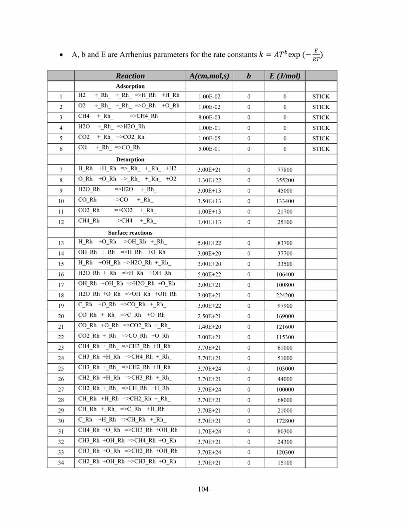
104
A, b and E are Arrhenius parameters for the rate constants exp
Reaction A(cm,mol,s) b E (J/mol)
Adsorption
1 H2 +_Rh_ +_Rh_ =>H_Rh +H_Rh 1.00E-02 0 0 STICK
2 O2 +_Rh_ +_Rh_ =>O_Rh +O_Rh 1.00E-02 0 0 STICK
3 CH4 +_Rh_ =>CH4_Rh 8.00E-03 0 0 STICK
4 H2O +_Rh_ =>H2O_Rh 1.00E-01 0 0 STICK
5 CO2 +_Rh_ =>CO2_Rh 1.00E-05 0 0 STICK
6 CO +_Rh_ =>CO_Rh 5.00E-01 0 0 STICK
Desorption
7 H_Rh +H_Rh =>_Rh_ +_Rh_ +H2 3.00E+21 0 77800
8 O_Rh +O_Rh =>_Rh_ +_Rh_ +O2 1.30E+22 0 355200
9 H2O_Rh =>H2O +_Rh_ 3.00E+13 0 45000
10 CO_Rh =>CO +_Rh_ 3.50E+13 0 133400
11 CO2_Rh =>CO2 +_Rh_ 1.00E+13 0 21700
12 CH4_Rh =>CH4 +_Rh_ 1.00E+13 0 25100
Surface reactions
13 H_Rh +O_Rh =>OH_Rh +_Rh_ 5.00E+22 0 83700
14 OH_Rh +_Rh_ =>H_Rh +O_Rh 3.00E+20 0 37700
15 H_Rh +OH_Rh =>H2O_Rh +_Rh_ 3.00E+20 0 33500
16 H2O_Rh +_Rh_ =>H_Rh +OH_Rh 5.00E+22 0 106400
17 OH_Rh +OH_Rh =>H2O_Rh +O_Rh 3.00E+21 0 100800
18 H2O_Rh +O_Rh =>OH_Rh +OH_Rh 3.00E+21 0 224200
19 C_Rh +O_Rh =>CO_Rh +_Rh_ 3.00E+22 0 97900
20 CO_Rh +_Rh_ =>C_Rh +O_Rh 2.50E+21 0 169000
21 CO_Rh +O_Rh =>CO2_Rh +_Rh_ 1.40E+20 0 121600
22 CO2_Rh +_Rh_ =>CO_Rh +O_Rh 3.00E+21 0 115300
23 CH4_Rh +_Rh_ =>CH3_Rh +H_Rh 3.70E+21 0 61000
24 CH3_Rh +H_Rh =>CH4_Rh +_Rh_ 3.70E+21 0 51000
25 CH3_Rh +_Rh_ =>CH2_Rh +H_Rh 3.70E+24 0 103000
26 CH2_Rh +H_Rh =>CH3_Rh +_Rh_ 3.70E+21 0 44000
27 CH2_Rh +_Rh_ =>CH_Rh +H_Rh 3.70E+24 0 100000
28 CH_Rh +H_Rh =>CH2_Rh +_Rh_ 3.70E+21 0 68000
29 CH_Rh +_Rh_ =>C_Rh +H_Rh 3.70E+21 0 21000
30 C_Rh +H_Rh =>CH_Rh +_Rh_ 3.70E+21 0 172800
31 CH4_Rh +O_Rh =>CH3_Rh +OH_Rh 1.70E+24 0 80300
32 CH3_Rh +OH_Rh =>CH4_Rh +O_Rh 3.70E+21 0 24300
33 CH3_Rh +O_Rh =>CH2_Rh +OH_Rh 3.70E+24 0 120300
34 CH2_Rh +OH_Rh =>CH3_Rh +O_Rh 3.70E+21 0 15100

105
35 CH2_Rh +O_Rh =>CH_Rh +OH_Rh 3.70E+24 0 158400
36 CH_Rh +OH_Rh =>CH2_Rh +O_Rh 3.70E+21 0 36800
37 CH_Rh +O_Rh =>C_Rh +OH_Rh 3.70E+21 0 30100
38 C_Rh +OH_Rh =>CH_Rh +O_Rh 3.70E+21 0 145500
106
VITA
Arman Raoufi completed the Bachelor of Science degree in Mechanical Engineering at
the Ferdowsi University of Mashhad and Master of Science degree in Mechanical Engineering at
the K.N. Toosi University of Technology in 2004 and 2006 receptively. After graduating, he
worked for one year at the K.N. Toosi University of Technology as a research assistant and then
joined renewable energy department of Niroo Research Institute where he worked on the design,
manufacturing and simulation of fuel cells for more four years. In 2011, he decided to pursue his
Ph.D. in Computational Engineering at the SimCenter, the University of Tennessee at
Chattanooga and earned his degree in 2016.