computational analysis of conjugate heat transfer and...

Proceedings of IGTI 2009

ASME Turbo Expo 2009: Power for Land, Sea, and Air June, 2009, Florida, United States

GT 2009- 59573

COMPUTATIONAL ANALYSIS OF CONJUGATE HEAT TRANSFER AND PARTICULATE DEPOSITION ON A HIGH PRESSURE TURBINE VANE

Weiguo Ai, Thomas H. Fletcher Department of Chemical Engineering, Brigham Young University, Provo, UT 84602

Proceedings of ASME Turbo Expo 2009: Power for Land, Sea and Air GT2009

June 8-12, 2009, Orlando, Florida, USA

GT2009-59573

1 1 Copyright © 2009 by ASME

ABSTRACT

Numerical computations were conducted to simulate flyash deposition experiments on gas turbine disk samples with internal impingement and film cooling using a CFD code (FLUENT). The standard k-ω turbulence model and RANS were employed to compute the flow field and heat transfer. The boundary conditions were specified to be in agreement with the conditions measured in experiments performed in the BYU Turbine Accelerated Deposition Facility (TADF). A Lagrangian particle method was utilized to predict the ash particulate deposition. User-defined subroutines were linked with FLUENT to build the deposition model. The model includes particle sticking/rebounding and particle detachment, which are applied to the interaction of particles with the impinged wall surface to describe the particle behavior. Conjugate heat transfer calculations were performed to determine the temperature distribution and heat transfer coefficient in the region close to the film-cooling hole and in the regions further downstream of a row of film-cooling holes. Computational and experimental results were compared to understand the effect of film hole spacing, hole size and TBC on surface heat transfer. Calculated capture efficiencies compare well with experimental results.

NOMENCLATURE A Surface area [m2] C particle specific heat [kJ/ (kg.K)] d hole diameter dp particle diameter D coupon diameter E Young Modulus [Pa] F force [N] Fpo sticking force [N] h convective heat transfer coefficient [W/m2 K] k kinetic energy per unit mass [J/kg] Kc Composite Young’s modulus ks Constant used in Eqn. 3 kt thermal conductivity [W/m K] m mass [kg] M blowing ratio=ρcUc/ρ∞U∞ M1 s/d=3.375, d=1 mm, metal coupon M2 s/d=4.5, d=1 mm, metal coupon M3 s/d=3, d=1.5 mm, metal coupon q″ heat flux [W/m2] s hole spacing [mm] T temperature

TADF turbine accelerated deposition facility TBC thermal barrier coating Tu turbulence intensity U velocity [m/s] uτc critical wall shear velocity [m/s] vc capture velocity [m/s] WA Constant used in the sticking force [J/m2] x spanwise coordinate from left edge of coupon y streamwise coordinate from film hole center ε turbulent dissipation rate [m2/s3] ω specific dissipation rate [s-1] α inclined angle of cooing holes [degrees] ρ density [kg/m3] η overall film cooling effectiveness Subscripts aw adiabatic wall b blackbody c property value of coolant for film cooling m property value of mainstream p property value of particle s target surface w wall ∞ feestream property INTRODUCTION

The continuous demand on performance improvement in gas turbine engines requires the engine components to be designed for higher combustor exit temperatures. Current advanced gas turbine engines operate at turbine rotor inlet temperatures 1200-1450°C (or 2200-2600°F), which is hot enough to melt or severely weaken critical areas of the engine downstream of the combustor. With the introduction of syngas derived from “dirty fuels” for replacing natural gas in a gas turbine system, small particles contained in the combustion product can accumulate on the component surface, resulting in severe adverse effects to gas turbine components. Component surface temperature is one of the significant factors determining whether or not a particular dust is deposited. Kim et al. [1] reported that the surface temperature onto which the particles impact must be above a certain threshold temperature if deposition is to occur. Increasing the vane metal temperature increases the amount of deposits significantly.

Film cooling is a common technique used in the gas turbine industry to prevent hot-section components from failing at elevated temperatures. The efficiency of this

technique depends on several parameters, such as the injection blowing ratio, mainstream characteristics, surface roughness, the spacing of the holes and their arrangement and injection angle. To design efficient cooling systems and mitigate particulate deposition, it is important to know the influence of a variety of parameters on the cooling performance and their correlation with particulate deposition to predict deposition development.

Brown and Saluja. [2] studied coolant injection through a single hole and rows of holes with three ratios of pitch to diameter. The greatest average effectiveness in the region close to the holes appeared for the smallest pitch to diameter ratio. Drost et al. [3] carried out an experimental work on film cooling effectiveness and heat transfer investigation on a flat plate. They reported that mainstream turbulence reduced flat plate effectiveness at low and moderate blowing ratios, but increased the effectiveness at high blowing ratios due to a better dispersion of the detaching jets in the boundary layer. For the effect of rows of cylindrical rows, Saumweber and Schulz [4] reported the second row hole shape and blowing ratio dominated film cooling performance downstream of two rows of holes. The upstream row holes increased film cooling effectiveness downstream of the second ejection locations.

A systematic computational methodology was developed by Walters and Leylek. [5] to calculate the adiabatic effectiveness of film cooling. Four critical issues to the success of a computational prediction were proposed: (i) computational model; (ii) geometry representation and grid generation; (iii) discretization scheme; and (iv) turbulence modeling. Their computational results tended to show that the use of unstructured grids over-predicted centerline effectiveness values and under-predicted the lateral average values, but showed more consistent agreement with experimental data than with a structured grid simulation. Hoda and Acharya [6] investigated the performance of several existing turbulence models on the prediction of film coolant jets in cross flow. Computational results were compared with measurements reported by Ajersch et al. [7] to examine whether the models accurately predicted the dominant features of flow field. The use of the k-ω model yielded an improved prediction of near-wall structures. Jia et al. [8] performed a systematic evaluation of the current computational model to study the film cooling fluid injection from slots or holes into a crossflow. They concluded that the shear stress transport k-ω model provided a more faithful prediction of the mean and rms velocity distribution. The 30° jet provided the highest film-cooling effectiveness. Harrison and Bogard [9] found that the standard k-ω (SKW) model best predicted laterally averaged adiabatic effectiveness, and that the realizable k-ε model was best along the centerline. The Reynolds stress model yielded the best predicted heat transfer coefficients.

In turbomachinery applications, the heat conduction inside the solid cannot be neglected. It is therefore necessary to consider the flow field together with temperature distributions within the metal. Bohn et al. [10] studied the calculations of a film-cooled duct wall with the boundary condition of an adiabatic and a conjugate heat transfer condition for various configurations of film-holes. The conjugate heat transfer was found to influence the velocity field within the cooling film. The magnitude of the peak secondary flow velocities was much higher for the adiabatic case than with the conjugate heat transfer, which degraded the performance of the cooling. Silieti et al. [11] predicted film cooling effectiveness using three different turbulence models: the realizable k-ε model (RKE); the SST k-ω model; and the v2-f model. They predicted that film effectiveness obtained from the conjugate model is in better agreement with the experimental data compared to the adiabatic model. Andreini et al. [12] carried out several calculations to infer the trends of adiabatic and conjugate heat transfer performance in terms of heat transfer coefficient,

2

overall and adiabatic effectiveness. They concluded that the reduction of metal temperature upstream of each cooling hole increased as the blowing rate grew. Na et al. [13] performed computations to study the conjugate heat transfer of a flat plate with and without TBC. They found that the surface temperature increased slightly when the thermal conductivity was reduced to a certain value.

Models of particle transport and deposition can be developed either by the Eulerian approach or the Langrangian approach. The first major deposition models using an Eulerian approach were developed by Friedlander and Johnstone [14], Davies. [15]. Liu and Agarwal [16] proposed a new expression for particle diffusivity, containing an additional term to account for enhanced deposition by inertia. The model yielded reasonable agreement with deposition rate measurements for intermediate particle relaxation times, but poor agreement at high relaxation times.

In the Lagrangian approach, a number of particle trajectories are simulated by solving the equations of continuity, momentum, and energy for individual representative particles. Multiple forces on the particle are considered in the particle equation of motion. This approach provides detailed information on particle collisions at the surface that are required for sticking studies. Kallio and Reeks [17] presented a Lagrangian approach to model particles transported in turbulent duct flows. They solved the equation of motion for particles with normalized relaxation times ranging from 0.3 to 1000. Their results showed very good agreement with the experimental data of Liu and Agarwal [16] over a wide range of particle sizes. Greenfield and Quarini [18] considered the drag force as the principal force acting on particles. They represented the effect of turbulence on the particles by using the eddy lifetime model.

The previous numerical simulations applied different methods in FLUENT package to study the secondary flow in the film cooling technology and compare the experimental results. Although the agreement is not made completely, the conclusions from them are still helpful to numerical model built-up here. This paper investigates film cooling effectiveness and heat transfer coefficients with both conjugate heat transfer and adiabatic conditions in the region close to film-cooling holes and in the region further downstream of a row of film-cooling holes, based on the unstructured grids and standard k-ω turbulence model. Comparisons are made between computational and experimental results to understand the effect of film hole spacing, hole size and TBC on surface heat transfer. After heat transfer calculation, particle capture efficiencies are calculated and compared with measured values to evaluate the performance of the ash particulate deposition model. The prediction combining those factors occurred in gas turbine is a meaningful try for film cooling art.

EXPERIMENTAL TEST CASE

The three-dimensional computational model is a simulation of the experiments performed in the turbine accelerated deposition facility (TADF). A complete description of the experimental facility including the test section, and instrumentation used in obtaining the temperature data is given by Ai et al. [19]. Only a brief summary is provided here. A 1 inch diameter coupon sample was exposed to a jet from a natural gas burning combustor at turbine relevant temperatures and the correct flow Mach number (Figure 1). The combustor was seeded with particulate to study deposition in an accelerated time. The bare metal sample was manufactured with three cylindrical holes spaced 4.5 mm apart at a 30 deg inclined angle relative to the free-stream. The diameter (d) of each hole was 1.5 mm. The middle hole exit was located in the center of the circular coupon, and the other two hole exits were located along a line of symmetry. The coupons were composed of Inconel alloy.

1 Copyright © 2009 by ASME

The coolant chamber simulates film cooling that is typically used in modern vanes and rotors. The coolant was heated to the appropriate temperature and entered the coolant chamber, impinged upon the backside of the coupon, and exited through the holes in the coupon. The design allows for coolant temperature measurement near the hole entrance

3

using a thermocouple mounted 4 mm behind the coupon and in the center of the coolant air flow. The gas and particulate impinged upon the coupon surface at a 45° angle. The rear and front surface temperature of the coupon were measured

Figure 1. Schematic of the BYU Turbine Accelerated Deposition Facility

Deposit-laden combustor exhaust

gas @1200C

25 mm diameter TBC-coated

target coupon

Radiation Shield

CoolantEntrance

Cap

Deposit-laden combustor exhaust

gas @1200C

25 mm diameter TBC-coated

target coupon

Radiation Shield

CoolantEntrance

Cap

using an RGB camera with a 2-color technique. The coupons employed in the experiments are described

in Table 1. The thickness of the TBC layer was 0.25 mm. The coolant was injected from the film cooling holes and its density ratio (ρc/ρ∞) is controlled by the heater. To study the effect of hole geometry, hole spacing and TBC, a series of tests were performed to measure surface temperature, capture efficiency, deposit pattern features and deposit thickness. Blowing ratios (M) of 0.5 to 4.0 were used with the density ratio maintained from 1.5 to 2.2.

Table 1. Coupon configuration category

Plate Material d α s/d

M1 Inconel 1 mm 300 3.375

M2 Inconel 1 mm 300 4.5

M3 Inconel 1.5 mm 300 3

TBC Nickel alloy with TBC 1 mm 300 4.5

DETAILS OF NUMERICAL SIMULATION Approach

Gas Phase Simulation Simulations were performed using FLUENT 6.3.26 with

Reynolds-averaged Navier-Stokes (RANS) transport equations and standard k-ω turbulent model [20, 21]. The continuity, momentum and energy equations in the fluid and solid regions were solved to predict velocity, temperature fields and film cooling effectiveness for conjugate heat film cooling from the holes. The interface between fluid and solid was specified as a coupled boundary, which avoided the use of the film cooling heat transfer boundary condition and allows a direct calculation of the heat transfer and wall temperature. The physical domain was separated into fluid

and solid blocks by the wall. The three dimensional Navier-Stokes equations and turbulence equations were solved in the fluid blocks. The Fourier equation was applied in the solid body blocks. Coupling of fluid blocks and solid blocks was achieved by equating the local heat fluxes passing through the common cell faces.

The SIMPLE algorithm was used to couple the pressure and velocity. Coefficients are determined by the QUICK scheme for the momentum equations. The discretization of the energy governing equation was performed using the first upwind scheme and the k-ω equation used the second upwind scheme. Convergence was determined by the orders of magnitude reduction of parameter residuals: 4 for continuity, 6 for velocity, 7 for energy, and 5 for turbulence quantities. Particle Phase Simulation

The Lagrangian approach was used for the particle phase. The two forces considered in the particle transport model are the drag force at steady state and the Saffman lift force. The trajectory of the particle is predicted by the integration of its equation of particle motion (shown here for the x-direction):

xppD

pp

p FuuC

ddtdu

+−= )(24Re18

2ρμ (1)

The first term on the right-hand side of this equation represents the drag force per unit particle mass, and Fx stands for Saffman lift force [22]. Phase changes of the particle are not taken into account. The equation of particle temperature is defined as:

)( ppcp

pp TTAhdt

dTCm −= ∞ (2)

The assumption is made that the particles have no effect on the fluid flow due to the low particle loading.

The El-Batsh deposition model [23] was employed in this


simulation to study the particle-wall interaction. This model determines the fraction of incident particles that remain on the surface, and consists of two interaction processes. One interaction is a pure mechanical interaction in the absence of the fluid force. It mainly determines the condition at which no rebound occurs and is called the sticking process. The other interaction is the detachment process, which is a fluid dynamic interaction between the fluid and the adhered particles. Detachment is related to the stability of the particles at the surface. Van der Waals force, electrostatic forces, and liquid bridges play a significant role during the process of particle sticking. In the case of particle deposition on gas turbine surfaces, the van der Waals force is the major contributor to the particle sticking force. The sticking force Fpo is calculated as:

pAspo dWkF = (3)

where WA [J/m2] is a constant which depends on the properties of the particle and of the surface (WA is also used in equation 5). ks is a constant equal to 3 π/4. The capture velocity in the present study is given by:

710

2

⎥⎥⎦

⎤

⎢⎢⎣

⎡=

pcr d

Ev (4)

where E is the Young’s modulus. The particle normal impact velocity is compared to the particle capture velocity. If the particle normal impact velocity is smaller than the capture velocity, the particle sticks. Otherwise, the particle rebounds and continues the trajectory until it leaves the domain or impacts the surface at another place.

The critical moment theory is applied to describe the mechanism of particle detachment from a surface. The critical wall shear velocity uτc is:

31

2 )(cp

A

p

Auc Kd

WdWC

uρτ = (5)

The particle will be removed from the surface if the turbulent flow has a wall friction velocity (= ρτω / , where τw is the wall shear stress) which is larger than uτc. The relevant parameters and more details regarding the interaction between the particles and the wall are stated in [23].

Since the particle phase is sufficiently dilute, particle-particle interactions and the effects of particle volume fraction on the gas phase are negligible. Geometry

A schematic of the computational domain to simulate the experiment is shown in Figure 2. The computational domain includes the coolant supply channel, the cylindrical cooling holes, and mainstream duct. The crossflow section is 39 mm in width, 36 mm in height and 81 mm in length. The row of three inclined film cooling holes with a 30 degree angle against the plate is located 36 mm downstream of the flat plate leading edge and 45 mm upstream of the fluid outlet. The hole diameter is 1.5 mm and hole spacing is 3 times that of the hole diameter for case M3 (refer to Ai et al. [19, 24]). The thickness of the plate is 3.5 mm and the length-to-diameter ratio L/d of coolant passage is 4. A high temperature circular gas jet with a diameter of 25.4 mm impinges on the flat plate with a 45° angle, and blends with the film cooling air, and then flows out at the exit located in the schematic to the right side of duct. The coolant fluid was injected from a tube with a diameter of 13.5 mm to a plenum located beneath the plate. The coolant plenum is 40.5 mm in height, 39 mm in width and 81 mm in length. The mainstream gas temperature was specified at 1453 K, and the

measured density ratio was matched by varying the temperature of the inlet coolant. Additional cases were performed with the same geometry except for different hole sizes and hole spacing.

Figure 2. Schematic of the overall computational

domain.

Grid Generation and Independence Geometry and the mesh grid were generated using

GAMBIT with unstructured tetrahedral topology grids, which consist of tetrahedral cells, as shown in Figure 3. The total number of computational cells was 475,034 for case M3 and 421,949 for cases M1 and M2. The accuracy of the computational model is strongly dependent upon the quantity and location of grids that resolve the relevant flow physics. To study grid-independence, three test grids were used to compute film cooling of the flat plate with conjugate heat transfer, with 475,034 to 1,551,455 cells. The centerline effectiveness downstream of the middle film hole is shown in Figure 4 for the grid-independence calculations. The finer mesh resulted in little change downstream in the region close to film holes (Y/d < 10). Therefore, due to computational time restrictions, the mesh with the lowest number of grids was adapted for subsequent computational cases.


Figure 3. Details of the grid used in the simulations.

0.7

0.6

0.5

0.4

0.3

0.2

0.1

0.0

Coo

ling

Effe

ctiv

enss

121086420

Y/d

475,034 Cells 658,455 Cells 1,551,655 Cells

Figure 4. Grid sensitivity study-centerline normalized temperature for the three grids. Boundary Conditions

Seven simulation cases were chosen to match the experimental test cases, as shown in Table 2. The boundaries were defined from experimental conditions. The mainstream inlet air velocity was set to 173 m/s and 1453 K for all cases. The k and ω profiles were specified using a uniform distribution corresponding to a turbulence intensity of 4.7% for most cases. The temperatures on the top and side walls of the mainstream duct were set to 900 K except for the wall close to the inlet, which was 300 K. The fluid viscosity was held constant constant at 1.79×10-5 kg/(m·s). The top and bottom walls of the solid plate are specified as a coupled wall in the FLUENT solver, which avoids specifying the heat flux or other boundary conditions. The surrounding walls of the solid plate were set to be adiabatic, requiring the heat flux to be in only one direction inside the solid plate. At the outflow boundary, the gradients of all flow variables with respect to the streamwise direction were set to zero, and the no-slip condition with wall function was applied at the walls. The temperature at the inlet of the coolant plenum was varied to obtain the measured density ratio in each experiment. The walls of the coolant plenum were set to be adiabatic. The gas was modeled with gas density as only a function of the fluid temperature.

Table 2 Summary of Cases Simulated*

Case Plate

Hot side Plate s/d TBC

kt of

SA/TBC

(W/m·K)

Blowing

Ratio

(M)

1 Conjugate M1 3.4 N/A 9/n.a. 0.5,1.0,2.0

2 Conjugate M2 4.5 N/A 9/n.a 0.5,1.0, 2.1

3 Conjugate M3 3.0 N/A 9/n.a 0.5,1.0,1.5,2.0

4 Adiabatic M2 4.5 N/A 0/n.a. 1.0

5 Adiabatic M3 3.0 N/A 0/n.a. 1.0

6 Conjugate TBC 4.5 Yes 9/1.78 1.0

7 Conjugate TBC 4.5 Yes 9/0.3 1.0

* kt is thermal conductivity. SA means super-alloy, vs. TBC.

In the deposition simulation, 5000 ash particles were released at the center of the mainstream inlet surface and impinged the target plate. The temperatures and velocities of the particles were initially set to the same values as the mainstream gas. The properties of the ash particles are listed in Table 3. The average size of particles in the simulation was 13.4 µm and the particle size bins complied with a Rosin-Rammler logarithm distribution. Particle trajectories and temperatures were modeled on a particle-by-particle basis in the stochastic random-walk model, which is based on the force balance on the particle and on the convective heat from the particle. The Runge-Kutta method was used to integrate the particle equations, and the Cunningham correction to Stokes’s drag law was also used. Each particle in the deposition simulation was tracked as it was carried through the computational domain by a combination of mean velocities and turbulent velocities calculated from k and ω.

Table 3 Particle properties

d(µm) ρ(kg/m3) Cp(J/kg·K) K(W/m·K) 13.4 990 984 0.5

RESULTS AND DISCUSSION

A. Young Modulus Determination The sticking model used here calculates the capture

velocity of the particle at the surface based on the van der Waals force. The capture velocity was determined by the size of the particle, temperature, and the material properties of the particle and target surface. An important model parameter in the model is the Young’s modulus (E), which is not available in the literature. Soltani and Ahmadi [25] documented that the value of E of a steel target surface is 2.15×1014 while E of particles ranges from 1×105 Pa to 1×1010 Pa. The E was obtained in this model by fitting experimental data. Experiments were performed in the TADF with gas temperatures varying from 1294 to 1453 K. The coupon was made of Inconel and the backside was insulated by ceramic material, resulting in adiabatic conditions. The ash-laden gas impinged upon the disk with a 45° angle. The capture efficiency was calculated as the deposit mass divided by the particle mass fed into the system.

Two-dimensional numerical computations were performed to solve the flow field and particle trajectories for this set of tests. A schematic of the model is presented in Figure 5. The model geometry included 30,100 cells. The inlet velocity was 173 m/s and the wall of the inlet tube was


adiabatic. All other walls were assumed as a pressure outlet with a temperature of 300 K, simulating atmospheric conditions.

Figure 5. Schematic of the 2D model.

When the particles arrive at the target surface, the sticking

model was applied to determine whether the particle sticks to the surface or escapes. To investigate the correlation of Young’s modulus with temperature, the model was tuned to fit the capture efficiency obtained in the experiments. The assumption was made that the particle sticking properties represent the target surface properties as well. The composite Young’s modulus was computed by setting the Poisson ratio to a constant value of 0.27 for both the particle and the surface [26].

The continuous-phase flow field was solved and the discrete-phase injection was tracked. As the particle impacted on the target surface, the particle temperatures and velocity were calculated as well. The capture velocities were calculated on the basis of the assumed value of the Young’s modulus. The particles with normal velocities less than the capture velocity stuck to the surface. The capture efficiency is the ratio of the mass of the adhered particles to the total mass of particles injected into the domain. The average between the particle temperature and the surface temperature was used to determine the properties for the deposition model. This process was iterated with different values of Ep until the capture efficiency in the model was in agreement with the result obtained in the experiments for each gas temperature. The dependence of Young’s modulus on the temperature was then fit to an exponential function, as shown in Equation 6. Figure 6 shows the calculated capture efficiency from the CFD model using Equation 6. Good agreement is shown with the experiments performed as a function of gas temperature.

)02365.0exp(103 20gp TE −×= (6)

Although particles can be delivered by the inertial force to the targeted surface, the deposition that occurs depends on whether particles stick upon arrival at the surface. To specify the effect of delivery and attachment on surface deposition, the capture efficiency is divided into two terms: impact efficiency and sticking efficiency. Impact efficiency is defined as the ratio of mass of particles impacting the surface to the total particle mass flowing into the system. Sticking efficiency is the ratio of the mass of particles sticking on the surface to the mass of impacted particles.

6

10

8

6

4

2

0

Cap

ture

Eff

icie

ncy

(%)

150014501400135013001250

Tg (K)

Model Experiment

Figure 6. Calculated capture efficiencies obtained from 2-D

CFD modeling versus measured values.

Figure 7 shows calculated impact efficiency, sticking efficiency and overall capture efficiency for different size-classes of particles. As can be seen, the impact efficiency is increases with particle size. For 8-10 µm diameter particles, the impaction efficiency in this experiment is close to 100%. This is due to the large Stokes number, which enables particles to maintain their trajectories and impact the target surface. The temperature has only a slight effect on impingement efficiency.

Equation 4 above shows that critical capture velocity of particles is inversely proportional to particle size, which indicates that small particles have a greater tendency to stick on the surface than large particles. Figure 7b shows that sticking efficiency decreases with increasing particle size. For particles larger than 10 µm, the efficiency is close to zero while for particles less than 2 µm, the efficiency is 100%. For a given particle size, the sticking efficiency increases with increasing temperature.

The capture efficiency for different particle sizes was obtained by multiplying the impact efficiency by the sticking efficiency, as shown in Figure 7c. At the lowest temperature of 1293 K, the peak capture efficiency appeared in the size range of 2-4 μm. At 1453 K, the peak is located in the range of 8 μm. The influence of temperature on deposition for various particle sizes is treated in the Young Modulus correlation (Eq. 6). The capture efficiency peak shifts to the larger sized particles with increased temperature. This result is consistent with the conclusion made by Wenglarz and Wright [27] who reviewed test results for a number of alternate fuels. Above the transition temperature, particles larger than 1 µm are molten. Due to the high delivery rate of large particles, a much greater mass of large particles stick on the surface, resulting in a significant increase in the mass of deposit.

0102030405060708090

100

0 2 4 6 8 10 12Particle Diameter d(um)

Impa

ct E

ffici

ency

T=1453KT=1425KT=1408KT=1374KT=1352KT=1293K

(a)


0102030405060708090

100110


Stic

king

Effi

cien

cy

T=1453KT=1425KT=1408KT=1374KT=1352KT=1293K

(b)

0

10

20

30

40

50

60


Cap

Eff

(%)

T=1453KT=1425KT=1408KT=1374KT=1352KT=1293K

(c)

Figure 7. 2-D CFD calculations of (a) impact efficiency, (b) sticking efficiency, and (c) capture efficiency versus particle size for various gas temperatures. B. Hole spacing (s/d=3.375 and 4.5)

To study the effect of hole spacing on film cooling, computations were made for two cases with hole spacings of s/d=3.4 (Case 1) and 4.5 (Case 2) for blowing ratios (M) from 0.5 to 2.0. Comparisons were made of predicted and measured average front and rear plate temperature (Figure 8) and deposition capture efficiency (Figure 9). The plate surface impinged by free stream is the front side while the plate surface on the coolant side is the back side. As can be seen in Figure 8, the predicted temperatures at M=2.0 for case 1 agrees with experiments better than at M=1.0. The predicted temperatures for both front and back sides at M=0.5 are higher than the measured values. For case 2, the predicted temperatures at M=0.5 and 2.0 are close to the experimental results while there is a slight disagreement at M=1.0. In general, the predictions for case 2 agreed with the data better than for case 1.

Figure 9 shows the deposition capture efficiency as the function of blowing ratio for varying hole spacing cases. This figure suggests that the deposition model predicts capture efficiency fairly accurately over this range of blowing ratios. The areas of disagreement shown in this figure reflect the areas of disagreement shown earlier for the respective plate surface temperature. Capture efficiency is over-predicted slightly for case 1 with M=0.5 and 1.0 due to a higher simulated surface temperature. The predicted capture efficiency for case 2 with M=1.0 is lower in the simulation than that obtained from experiments. This figure also shows that the capture efficiency for close hole spacing is slightly lower than for wide hole spacing.

The use of an overall effectiveness factor is a method of normalizing the temperature, and is defined as:

7

1400

1300

1200

1100

1000

Tem

pera

ture

(K

)

2.52.01.51.00.50.0

Blowing Ratio (M)

s/d = 3.375 4.5 CFD Front Exp Front CFD Back Exp Back

Figure 8. Comparison of averaged front-side and backside plate temperature for cases s/d=3.4 and 4.5 from experiment and 3-D modeling

6

5

4

3

2

1

0

Cap

ture

Effi

cien

cy (

%)

2.52.01.51.00.50.0

Blowing Ratio (M)

Model Exp s/d = 3.375 s/d = 4.5

Figure 9. Capture efficiency at M=0.5 to 2.0 for cases s/d=3.4 and 4.5 from experiment and 3-D modeling

mc

m

TTTT

−−

=η (7)

where T is the wall surface temperature downstream of film holes, Tc is the coolant temperature at the entry of the passage of the holes and Tm is the mainstream temperature. The laterally averaged effectiveness is obtained by spanwise averaging of the local values. This evaluation is performed for the downstream range from Y/d=1 to 12, where Y = 0 at the hole axis. The diameter of coupons used in experiment is 25.4 mm. Therefore, only the local points within a radius of less than 12.7 mm are averaged.

Figure 10 shows the results of the laterally averaged effectiveness for a variation of the blowing ratio from 0.5 to 2.0 with the two differing hole spacings. The curves reflect the effects of three cooling air jets interacting with each other and mixing with hot gas crossflow. The figure shows that cooling effectiveness rises with the increase of blowing ratio. The development of lateral effectiveness with downstream distance continuously decays due to the interaction with the hot mainstream after ejection from the cooling holes. The different hole spacing causes a slight variation in the downstream decay characteristic, which develops more rapidly for a plate with a wider hole spacing. The cooling effectiveness for the plate with wide hole spacing is larger than the case with close hole spacing at all blowing ratios in the location near cooling holes. Due to less support of neighboring coolant jets with large hole spacing, the coolant flow is diluted by the hot gas flow at the region far away from the cooling holes, resulting in a lower cooling effectiveness than the close spacing at the Y/d greater than


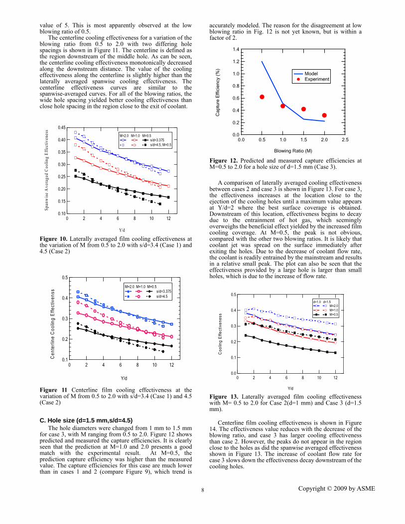
value of 5. This is most apparently observed at the low blowing ratio of 0.5.

The centerline cooling effectiveness for a variation of the blowing ratio from 0.5 to 2.0 with two differing hole spacings is shown in Figure 11. The centerline is defined as the region downstream of the middle hole. As can be seen, the centerline cooling effectiveness monotonically decreased along the downstream distance. The value of the cooling effectiveness along the centerline is slightly higher than the laterally averaged spanwise cooling effectiveness. The centerline effectiveness curves are similar to the spanwise-averaged curves. For all of the blowing ratios, the wide hole spacing yielded better cooling effectiveness than close hole spacing in the region close to the exit of coolant.

0.45

0.40

0.35

0.30

0.25

0.20

0.15

0.10

Span

wis

e A

vera

ged

Coo

ling

Effe

ctiv

enes

s

121086420

Y/d

M=2.0 M=1.0 M=0.5 s/d=3.375 s/d=4.5, M=0.5

Figure 10. Laterally averaged film cooling effectiveness at the variation of M from 0.5 to 2.0 with s/d=3.4 (Case 1) and 4.5 (Case 2)

0.5

0.4

0.3

0.2

0.1Cen

terl

ine

Coo

ling

Effe

ctiv

enss

121086420

Y/d

M=2.0 M=1.0 M=0.5 s/d=3.375 s/d=4.5

Figure 11 Centerline film cooling effectiveness at the variation of M from 0.5 to 2.0 with s/d=3.4 (Case 1) and 4.5 (Case 2) C. Hole size (d=1.5 mm,s/d=4.5)

The hole diameters were changed from 1 mm to 1.5 mm for case 3, with M ranging from 0.5 to 2.0. Figure 12 shows predicted and measured the capture efficiencies. It is clearly seen that the prediction at M=1.0 and 2.0 presents a good match with the experimental result. At M=0.5, the prediction capture efficiency was higher than the measured value. The capture efficiencies for this case are much lower than in cases 1 and 2 (compare Figure 9), which trend is

8

accurately modeled. The reason for the disagreement at low blowing ratio in Fig. 12 is not yet known, but is within a factor of 2.

1.4

1.2

1.0

0.8

0.6

0.4

0.2

0.0

Cap

ture

Effi

cien

cy (

%)

2.52.01.51.00.50.0

Blowing Ratio (M)

Model Experiment

Figure 12. Predicted and measured capture efficiencies at M=0.5 to 2.0 for a hole size of d=1.5 mm (Case 3).

A comparison of laterally averaged cooling effectiveness between cases 2 and case 3 is shown in Figure 13. For case 3, the effectiveness increases at the location close to the ejection of the cooling holes until a maximum value appears at Y/d=2 where the best surface coverage is obtained. Downstream of this location, effectiveness begins to decay due to the entrainment of hot gas, which seemingly overweighs the beneficial effect yielded by the increased film cooling coverage. At M=0.5, the peak is not obvious, compared with the other two blowing ratios. It is likely that coolant jet was spread on the surface immediately after exiting the holes. Due to the decrease of coolant flow rate, the coolant is readily entrained by the mainstream and results in a relative small peak. The plot can also be seen that the effectiveness provided by a large hole is larger than small holes, which is due to the increase of flow rate.

0.5

0.4

0.3

0.2

0.1

0.0

Coo

ling

Effe

ctiv

enes

s

121086420

Y/d

d=1.0 d=1.5 M=2.0 M=1.0 M=0.5

Figure 13. Laterally averaged film cooling effectiveness with M= 0.5 to 2.0 for Case 2(d=1 mm) and Case 3 (d=1.5 mm).

Centerline film cooling effectiveness is shown in Figure

14. The effectiveness value reduces with the decrease of the blowing ratio, and case 3 has larger cooling effectiveness than case 2. However, the peaks do not appear in the region close to the holes as did the spanwise averaged effectiveness shown in Figure 13. The increase of coolant flow rate for case 3 slows down the effectiveness decay downstream of the cooling holes.


0.5

0.4

0.3

0.2

0.1

0.0

Coo

ling

Effe

ctiv

enss

121086420

Y/d

d=1.0 d=1.5 M=2.0 M=1.0 M=0.5

Figure 14. Centerline film cooling effectiveness with the variation of M from 0.5 to 2.0 for Case 2(d=1 mm) and Case 3 (d=1.5 mm)

9

The flow fields results for M=0.5 to 2.0 for cases 2 and 3 are shown in Figure 15. The computed velocity magnitude contours are obtained along the centerline plane (y=0) and their scales are different. Velocity gradients in the cooling hole passage are apparent in each case. The exit velocity from the large holes is less than that from the small holes, due to a slight difference in predicted gas temperature at the hole exit. The large hole case has a higher coolant mass flow rate to maintain the same blowing ratio. Jet penetration into the region just above the hole exit and slightly downstream is greater for the larger diameter hole case. The formation of a boundary layer is more apparent for the M=1.0 and 0.5 cases. Vertical slices of the gas temperature distribution near the center cooling hole at a downstream location of X/d = 2 are shown in Figure 16 for cases 2 and 3. The jet lift-off can be observed to occur at M=2.0 for case 3 (Figure 16b), since the low temperature core of the jet is lifted slightly above the coupon surface. The temperature map just downstream of the small hole simulation (Figure 16a) shows that the coolant jet core is closer to the wall and avoided lift-off.

(a) d=1 mm, s/d=4.5 (b) d=1.5 mm, s/d=3 Figure 15. Velocity magnitude contours (m/s) with blowing ratio from 0.5 to 2.0 along centerline plane for case 2 and 3.

(a) d=1.0 mm, s/d=4.5, M=2.0 (case 2) (b) d=1.5 mm, s/d=3.0, M=2.0 (case 3)

Figure 16. Gas temperature distribution in X/d=2 for case 2 and 3. Temperatures are in Kelvin.

M=2.0

M=1.0

M=0.5

M=2.0

M=1.0

M=0.5


D. Effect of conjugate heat transfer This section discusses the predicted effect of conjugate

heat transfer. The thermal conductivity of the plate was set to a value close to zero for the adiabatic conditions. Cases 4 and 5 are the adiabatic simulations corresponding to cases 2 and 3 with M=1.0. Comparison of the adiabatic cases with the conjugate heat transfer cases shows the influence of heat transfer through the coupon on the film cooling effectiveness.

Figure 17 compares the temperature contours of the entire hot surface for the adiabatic and conjugate conditions (cases 2 and 4). For the adiabatic case, the surface temperature approaches the hot gas temperature except in the flow paths of the coolant jets. Low surface temperatures are observed near the hole exits. When conjugate heat transfer is taken into account, the average surface temperature is significantly lower than the adiabatic wall case, especially in the regions uncovered by coolant. The decrease in surface temperature is caused by both film cooling and internal cooling from backside impingement on the coupon.

Figure 17. Surface temperature profiles of the coupon surface for M=1.0 from the adiabatic and conjugate predictions. Hole diameters were 1.0 mm. Temperatures are in Kelvin.

Figure 18 shows the laterally-averaged film cooling

effectiveness versus the distance downstream of the cooling holes for cases 4 and 5. It is apparent that the conjugate case has a higher value, representing better cooling performance than the adiabatic case for both hole diameter sizes. An effectiveness peak appears at the location of Y/d=1.0 for cooling holes with large sizes. Effectiveness for the adiabatic case decays more rapidly than for the conjugate case. This is because of temperature increase of the hot surface in the region far downstream of the holes. For the conjugate case, this increase is suppressed by the internal cooling.

0.45

0.40

0.35

0.30

0.25

0.20

0.15

0.10

0.05

0.00

Coo

ling

Effe

ctiv

enes

s

121086420

Y/d

d=1.5 d=1.0 conjugate adiabatic

Figure 18. Laterally averaged film cooling effectiveness at M=1.0 for adiabatic and conjugate cases.

Adiabatic

Conjugate

1

Figure 19 shows centerline film cooling effectiveness at M=1.0 for both the adiabatic case and the conjugate heat transfer case. In the adiabatic condition, the coolant jet is not heated up by the plate wall before exiting the hole and hence maintains the coolant inlet temperature. Therefore, the cooling effectiveness approaches 1.0 at the exit of the holes. However, a rapid decay of the effectiveness is shown downstream of the holes as the mainstream hot gas entrains with the coolant in the film. In the conjugate condition, the coolant is heated as it impinges on the cooler side of the coupon. Additional heat transfer occurs during passage through the holes, which leads to an additional temperature increase compared to the adiabatic condition. As a result, the film cooling effectiveness at the exit of the jet is 0.4 to 0.5, much lower than the adiabatic condition. Due to a slower decay, the conjugate condition outperforms the adiabatic cases at a distance Y/d > 8.

1.0

0.8

0.6

0.4

0.2

0.0

Coo

ling

Effe

ctiv

enes

s

121086420

Y (mm)

d =1.5 d=1.0 Adiabatic Conjugate

Figure 19. Centerline effectiveness at M=1.0 for adiabatic and conjugate case.

In the conjugate heat transfer condition, the convective heat load to the hot coupon surface is given by:

)( waw TThq −=′′ (8)

where Taw is the surface temperature at each location from the adiabatic prediction. Figure 20 illustrates the change in the heat transfer coefficient along the distance downstream of the film cooling hole for different hole sizes. Generally, a cooling jet injected into a mainstream flow generates high levels of turbulence, which increases the local convective heat transfer coefficient. This trend dwindles with the further mixing of mainstream. Therefore, the heat transfer coefficient at the location close to the jets is at a maximum value of 240 W/ (m2·K). On account of the lower temperature of coolant directly downstream of the hole exit the coolant has a lower temperature than the surface temperature, so heat is transferred from the surface to the coolant. Further downstream, coolant mixes with the hot gas, and the gas mixture near the surface is heated up to a higher temperature than the surface. Heat is then transferred from the gas to the wall. The positive heat transfer coefficient shown in Figure 20 indicates that heat flows from the wall to the coolant stream. At Y/d<7, heat transfer coefficient value for holes with small and large sizes are similar, while at the further distances, the value of h has more rapid decay than for the smaller hole case.


250

200

150

100

50

0

h (W

/m2 K

)

1086420

Y/d

d=1.5 d=1.0

Figure 20. Centerline conjugate heat transfer coefficient for cases 2 and 3 with M=1.0. E. TBC Effect (d=1.0 mm, s/d=4.5)

A TBC layer with a thickness of 0.25 mm was added to the coupon surface, and the thermal conductivity (k) of the TBC layer was set to 1.78 W/m·K for case 6 and 0.3 W/m·K for case 7. Predictions were performed to examine the effect of a TBC layer on the metal surface temperature. A comparison of predictions obtained for cases 2, 4, 6 and 7 is shown in Figures 21 and 22. Note that with the addition of an insulating TBC layer (Case 6), the centerline and laterally averaged surface temperature along the centerline was reduced 50 K, compared to the case without TBC. However, with the thermal conductivity decreasing from 1.78 to 0.3, metal surface temperature does not continue to reduce but instead had an increase of 40 K, still less than the surface temperature from the case without TBC. This simulation result of first decreasing then increasing surface temperature with decreasing thermal conductivity coincides with Na’s study [13]. When k = 0, the temperature curve in Figure 22 crosses the curves from the other cases and elevates to a higher temperature than the other cases at location Y/d>5. Experiments to study the effect of TBC [24] show that the measured surface temperature for the TBC coupon was higher than the bare metal coupon. The temperature map was measured after a few minutes in the deposition test, so that the TBC surface had already captured some fine particles. Since the thermal conductivity of ash is as low as 0.1 to 0.2 W/(m·K) [28], the coupon thermal resistance is close to adiabatic condition, possibly resulting in a surface temperature which is higher than the same experiment with a bare metal surface. The increase of surface temperature speeds up the deposit formation and further decreases conductive heat transfer.

1400

1200

1000

800

600

400

200

Cen

terli

ne S

urfa

ce T

empe

ratu

re (

K)

121086420

Distance (inches)

Conjugate TBC,k=0.3 TBC,k=1.78 Adiabatic

Figure 21. Centerline surface temperature for M=1.0 with a TBC layer and different values of thermal conductivity.

11

1400

1350

1300

1250

1200

1150

1100

Ts

(K)

121086420

Y/d

Conjugate TBC, k=0.3 TBC, k=1.78 Adiabatic

Figure 22. Laterally averaged surface temperature for M=1.0 with a TBC layer with different values of thermal conductivity. SUMMARY AND CONCLUSIONS

3-D numerical simulations of film cooling fluid injection through a row of different- sized cylindrical holes distributed at varying hole spacing were performed using FLUENT at blowing ratios from 0.5 to 2.0. Simulations used RANS and the k-ω turbulence model to compute the flow field and heat transfer to a metal coupon for three cases: (a) adiabatic, (b) conjugate heat transfer and (c) a TBC layer. The boundary conditions were set to be those measured in an experimental facility (the TADF). Comparisons of film cooling effectiveness and heat transfer coefficients were presented to illustrate the effects of hole size, hole spacing, conjugate heat transfer and TBC layer on film cooling heat transfer. A series of particle-laden flow calculations were performed using a 2-D Lagrangian model. Model predictions were compared to deposition capture efficiency from new temperature-dependent experiments to determine a correlation for the particle Young’s Modulus (Ep) for this system. This correlation was then used in 3-D computations of ash particulate deposition for experiments with film cooling at different blowing ratios. User-defined subroutines were developed to describe particle sticking/rebounding and particle detachment on the impinged wall surface. Conclusions are as follows:

1. Results from the 2-D deposition model indicated that the small particles have a greater tendency to stick to the surface in the TADF experiments. After the initial deposition, and as the surface of the deposit rises above the transition temperature, large particles dominate the excessive deposition due to the high delivery rate, which is in agreement with the experimental results.

2. Predictions with the 3-D deposition model, using the correlation developed for the particle Young’s modulus, generally agree well with measured capture efficiencies for different blowing ratios and different hole sizes. Capture efficiency decreases with increased blowing ratio and increased hole size (when blowing ratio is held constant).

3. Predictions of the TADF experiments with different hole spacings (s/d=3.4 and 4.5) indicated that the averaged spanwise and centerline cooling effectiveness rises with the increase of blowing ratio. The effectiveness at locations close to the exit of jets for wide hole spacing is slightly higher than for small hole spacing. Meanwhile, the small hole spacing performed better than wide hole spacing at downstream locations due to the interaction of neighboring jets.

4. Predictions of the TADF experiments with different hole sizes indicated that the larger hole (1.5 mm) provides better cooling than a small hole (1 mm) based on centerline and averaged spanwise film cooling effectiveness. A small peak in the cooling effectiveness curve appears just downstream of the large holes, indicting jet lift off, especially at high blowing ratios.


5. Conjugate heat transfer calculations indicated that backside impingement cooling in the TADF experiments improved the overall cooling effectiveness, especially in the region far downstream of the cooling holes. The centerline heat transfer coefficient was predicted to decrease with distance downstream of the holes.

6. The addition of a TBC layer will effectively reduce the outer surface temperature initially. As a thin ash deposition layer forms with low thermal conductivity, the thermal resistance layer ultimately increases the outer surface temperature. The increase in surface temperature speeds up the deposit formation and further decreases conductive heat transfer ACKNOWLEDGEMENTS

This work was partially sponsored by the US Department of Energy – National Energy Technology Laboratory through a cooperative agreement with the South Carolina Institute for Energy Studies at Clemson University. The views expressed in this article are those of the authors and do not reflect the official policy or position of the Department of Energy or U.S. Government. REFERENCES [1] Kim, J., Dunn, M.G., Baran, A.J., Wade, D.P., and

Tremba, E.L., 1993, "Deposition of Volcanic Materials in the Hot Sections of Two Gas Turbine Engines," Journal of Engineering for Gas Turbines and Power, 115(3), pp. 641-651.

[2] Brown, A. and Saluja, C.L., 1979, "Film Cooling from a Single Hole and a Row of Holes of Variable Pitch to Diameter Ratio," International Journal of Heat and Mass Transfer, 22(4), pp. 525-534.

[3] Drost, U., Bolcs, A., and Hoffs, A., 1997, "Utilization of the Transient Liquid Crystal Technique for Film Cooling Effectiveness," ASME Paper No. 97-GT-26.

[4] Saumweber, C. and Schulz, A., 2003, "Interaction of Film Cooling Rows: Effects of Hole Geometry and Row Spacing on the Cooling Performance Downstream of the Second Row of Holes," Paper No. GT2003-38195.

[5] Walters, D.K. and Leylek, J.H., 1996, "Systematic Computational Methodology Applied to a Three-Dimensional Film-Cooling Flowfield," International Gas Turbine and Aeroengine Congress & Exhibition, Birmingham, UK.

[6] Hoda, A. and Acharya, S., 2000, "Predictions of a Film Coolant Jet in Crossflow with Different Turbulence Models," Journal of Turbomachinery, 122(3), pp. 558-569.

[7] Ajersch, P., Zhou, J.-M., Ketler, S., Salcudean, M., and Gartshore, I.S., 1995, "Multiple Jets in a Crossflow: Detailed Measurements and Numerical Simulations," International Gas Turbine and Aeroengine Congress and Exposition, Houston, TX, USA.

[8] Jia, R., Sunden, B., Miron, P., and Leger, B., 2005, "A Numerical and Experimental Investigation of the Slot Film-Cooling Jet with Various Angles," Journal of Turbomachinery, 127(3), pp. 635-645.

[9] Harrison, K.L. and Bogard, D.G., 2008, "Comparison of Rans Turbulence Models for Prediction of Film Cooling Performance," ASME Paper No.

1

GT2008-51423. [10] Bohn, D., Ren, J., and Kusterer, K., 2003, "Conjugate

Heat Transfer Aanalysis for Film Cooling Configurations with Different Hole Geometries," ASME Paper No. GT2003-38369.

[11] Silieti, M., Kassab, A.J., and Divo, E., 2005, "Film Cooling Effectiveness from a Single Scaled-up Fan-Shaped Hole a Cfd Simulation of Adiabatic and Conjugate Heat Transfer Models," Paper No. GT2005-68431.

[12] Andreini, A., Carcasci, C., Gori, S., and Surace, M., 2005, "Film Cooling System Numerical Design: Adiabatic and Conjugate Analysis," ASME Summer Heat Transfer Conference, San Francisco, CA, United States, 3.

[13] Na, S., Williams, B., Dennis, R.A., Bryden, K.M., and Shih, T.I.P., 2007, "Internal and Film Cooling of a Flat Plate with Conjugate Heat Transfer," Paper No. GT2007-27599.

[14] Friedlander, S.K. and Johnstone, H.F., 1957, "Deposition of Suspended Particles from Turbulent Gas Streams," Industry of Chemical Engineering, v 49, pp. p1151-1157.

[15] Davies, C.N., 1966, "Deposition from Moving Aerosols," In Aerosol Science, Academic Press.

[16] Liu, B. and Agarwal, J., 1974, "Experimental Observation of Aerosol Deposition in Turbulent Flow," Aerosol Science, 5, pp. 145.

[17] Kallio, G.A. and Reeks, M.W., 1989, "A Numerical-Simulation of Particle Deposition in Turbulent Boundary-Layers " International Journal of Multiphase Flow, 15(3), pp. 433-446.

[18] Greenfield, C. and Quarini, G., 1997, "Particle Deposition in a Turbulent Boundary Layer, Including the Effect of Thermophoresis," ASME Fluids Engineering Division Summer Meeting, Vancouver, Can, 17.

[19] Ai, W.G., Harding, S., Murray, N., Fletcher, T.H., Lewis, S., and Bons, J.P., 2008, "Deposition near Film Cooling Holes on a High Pressure Turbine Vane," ASME Paper No. GT2008-50901.

[20] 2005, Fluent 6.2 User Guide. Fluent Inc. [21] Wilcox, D.C., 1998, Turbulence Modeling for Cfd.

DCW Industries, Inc., La Canada, California. [22] 2005, Fluent 6.2 User Guide, pp. 23-5 to 23-10. [23] El-Batsh, H. and Haselbacher, H., 2002, "Numerical

Investigation of the Effect of Ash Particle Deposition on the Flow Field through Turbine Cascades," ASME Paper No. GT-2002-30600.

[24] Ai, W.G., Harding, S., Murray, N., Fletcher, T.H., and Bons, J.P., 2009, "Effect of Hole Spacing on Deposition of Fine Coal Flyash near Film Cooling Holes," ASME Paper No. GT2009-59569.

[25] Soltani, M. and Ahmadi, G., 1994, "On Particle Adhesion and Removal Mechanisms in Turbulent Flows," Adhesion Science Technology 8(7), pp. 763-785.

[26] Ai, W., 2009, "Deposition of Particulate from Coal-Derived Syngas on Turbine Blades with Film Cooling," PhD Dissertation, in progress, Chemical Engineering, Brigham Young University, Provo, UT.


[27] Wenglarz, R.A. and Wright, I.G., 2003, Alternate Fuels for Land-Based Turbines, in Materials and Practices to Improve Resistance to Fuel Derived Environmental Damage in Land- and Sea-Based Turbines, pp. 4-45 to 4-64.

[28] Robinson, A.L., Buckley, S.G., and Baxter, L.L., 2001, "Experimental Measurements of the Thermal Conductivity of Ash Deposits: Part 1. Measurement Technique," Energy & Fuels, 15(1), pp. 66(9).


computational analysis of conjugate heat transfer and...

Documents