computational ⊗⊘ photographygraphics.stanford.edu/courses/cs478/lectures/... · ⊕⊖...
TRANSCRIPT

⊕⊖ Computational ⊗⊘ Photography
Denoising
Jongmin Baek
CS 478 LectureFeb 13, 2012
Monday, February 13, 12

Announcements• Term project proposal
• Due Wednesday
• Proposal presentation
• Next Wednesday
• Send us your slides (Keynote, PowerPoint, etc)
• 4 minutes per group
• Assignment #2 grading
• Sign up at Rm. 360.
Monday, February 13, 12

Overview
• Noise model
• Image priors
• Self-similarity
• Sparsity
• Algorithms
• Non-local Means
• BM3D
Monday, February 13, 12

Noise• Every observation incurs some uncertainty.
Ground truth Observation
Monday, February 13, 12

Noise• Every observation incurs some uncertainty.
ISO 1600
Monday, February 13, 12

Source of Noise
• Photon shot noise
• Read noise
• Thermal noise
• Pixel non-uniformity
• Processing artifacts (demosaicking, JPEG)
• ...
Monday, February 13, 12
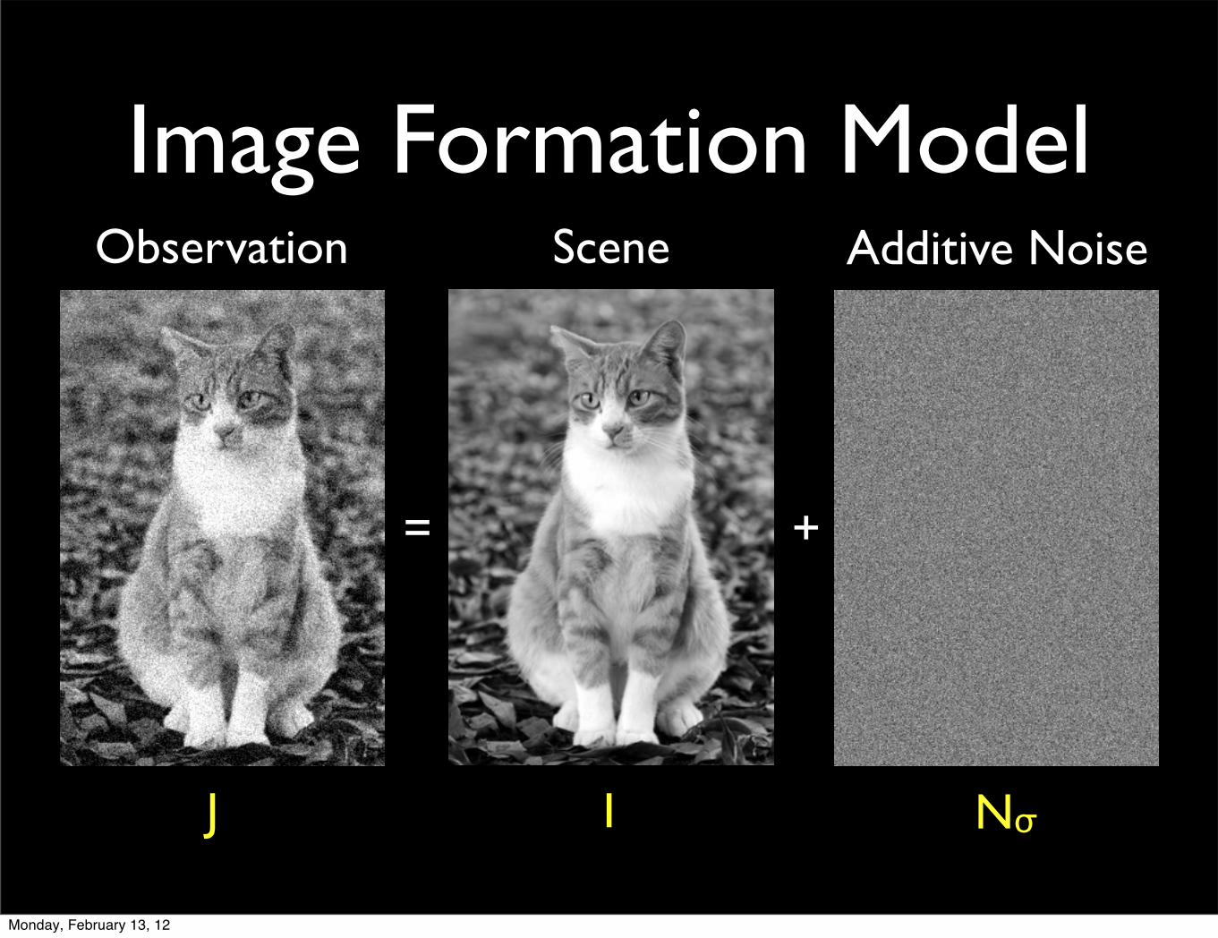
Image Formation ModelScene Additive Noise
+
Observation
=
J I Nσ
Monday, February 13, 12

Aside: Why Gaussian?
• Too many noise sources to model individually.
• Sum of random variables tend to a Gaussian distribution.
• Denoising algorithms exist for other models.
Monday, February 13, 12

Problem
• Given J, compute I (and N.)
• More unknowns than constraints!
Scene Noise
+
Observation
=
J I N
Monday, February 13, 12

Image Priors
• Images are not just random collection of intensity values.
• High correlations among nearby pixels
• Denoise by averaging with nearby pixels?
Monday, February 13, 12

Gaussian Filter• Gaussian of stdev 5
• Noise is gone, but so is detail.
Monday, February 13, 12

Image Priors
• Images are not just random collection of intensity values.
• High correlations among nearby pixels
• Denoise by averaging with nearby pixels?
• Denoise by averaging with nearby pixels of similar color?
Monday, February 13, 12

Bilateral Filter• Bilateral filter with σx=σy=10, σr=0.2
• Better, but still not great when noise is high.
Monday, February 13, 12

Image Priors
• Images are not just random collection of intensity values.
• Denoise by averaging with nearby pixels?
• Denoise by averaging with nearby pixels of similar color?
• Denoise by averaging with nearby pixels of similar texture?
Monday, February 13, 12
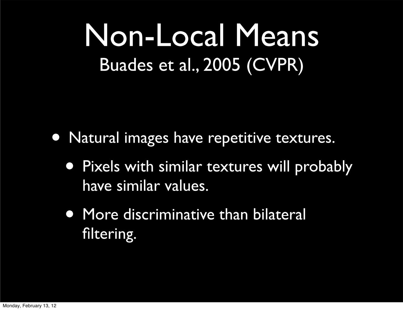
Non-Local MeansBuades et al., 2005 (CVPR)
• Natural images have repetitive textures.
• Pixels with similar textures will probably have similar values.
• More discriminative than bilateral filtering.
Monday, February 13, 12

How-to: NL-Means• It turns out this can be ensconced in the
Gaussian filtering framework.
• Here p(x) is the image patch centered at x, in a vectorized form.
v’(x) = ∑’y v(y) f( p(x) - p(y) )
Monday, February 13, 12

How-to: NL-Means
• For every x,
• Compute vector p(x).
• For every neighbor y,
• Compute vector p(y).
• Calculate the weight exp( -|p(x)-p(y)|2 / 2σ2 )
• Do the weighted sum.
v’(x) = ∑’y v(y) f( p(x) - p(y) )
Only look at 21x21 window around x
7x7 patch around pixel,so 49-dim vector
Monday, February 13, 12

How-to: NL-Means
• Slow part
• Calculate, for every pair (x,y),
|p(x)-p(y)|2
• Sum of squared difference between two patches.
v’(x) = ∑’y v(y) f( p(x) - p(y) )
Monday, February 13, 12

Calculating SSD
∑i ∑j | Ax(i,j) - Ay(i,j) |2
= ∑i ∑j Ax2(i,j) + ∑i ∑j Ay2(i,j) - 2 ∑i ∑j Ax(i,j)Ay(i,j)
Ax Ay
Easy with integral image
Same as Ax⊗Ay⟙
Monday, February 13, 12

NL-Means with FFT
• Compute the integral image of v2.
• For every x,
• Compute Ax.
• Compute ⨍-1{ ⨍{Ax} ⨍{v} }
• For every neighbor y,
• Calculate the weight exp( -|p(x)-p(y)|2 / 2σ2 )
• Do the weighted sum.
v’(x) = ∑’y v(y) f( p(x) - p(y) )
Simulates Ax⊗Ay⟙ for all y
Monday, February 13, 12

NL-Means with FFT
RuntimeN = # of pixels, M = dim. of p-space
Naive O(N2M)
With FFT O(N2logN)
Monday, February 13, 12

NL-Means with FFT
RuntimeN = # of pixels, M = dim. of p-space
Naive O(N N’ M)
With FFT O(N (N’+M) log (N’+M))
when neighbor search is restricted to N’
Monday, February 13, 12

NL-Means Filter
• Why does it work better than bilateral?
Monday, February 13, 12

Even Faster NL-Means
• Last time, we discussed how to make Gaussian filters very, very fast.
• Applicable here as well?
Monday, February 13, 12

Challenges
• p is very high-dimensional.
• Time complexity of our filtering algorithms scale with dimensionality of p.
• Can we lower the dimensionality of p?
v’(x) = ∑’y v(y) f( p(x) - p(y) )
Monday, February 13, 12

Patch Space
• Not all values in the p-space are equally plausible.
• There are subspaces that are much more likely.
• PCA to reduce dimensionality?
v’(x) = ∑’y v(y) f( p(x) - p(y) )
Monday, February 13, 12

PCA on Patches
• Generate the p-vectors for all pixels.
• High dimensional! (e.g. 147 if 7x7 patch on 3-channel img)
• Perform PCA to identify commonly occurring subspaces.
• Perhaps find ~6 principle components.
• Project the p-vectors onto this subspace.
• Voilà.
v’(x) = ∑’y v(y) f( p(x) - p(y) )
Monday, February 13, 12

PCA on PatchesSix principal components from the cat image
Monday, February 13, 12
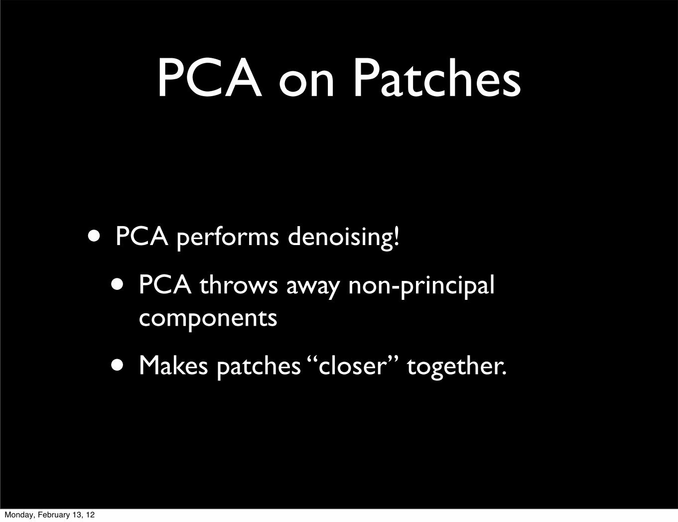
PCA on Patches
• PCA performs denoising!
• PCA throws away non-principal components
• Makes patches “closer” together.
Monday, February 13, 12

NL-Means Filter
Monday, February 13, 12

NL-Means: Analysis
• Find similar patches and average them.
• Should we do something besides averaging?
Monday, February 13, 12

Wavelet Shrinkage
• Hypothesis
• There exists a transform T such that applying T to patches will admit a sparse representation.
• This is useful in compression.
• DCT in JPEG encoding.
• PCA in NL-Means dimensionality reduction.
Monday, February 13, 12

Wavelet Shrinkage
• Take a patch in the image.
• Apply Haar wavelet transform
Monday, February 13, 12

Haar Wavelet Transform
Average pairs. Duplicate to upsample
1 0 2 4 1 3 1 0
0.5 3 2 0.5
1.75 1.25
1.5
Monday, February 13, 12

Haar Wavelet Transform
Average pairs. Duplicate to upsample
1 1 1 1 1 1 0 0
1 1 1 0
1 0.5
0.5
Monday, February 13, 12

Haar Wavelet Transform
Average pairs. Duplicate to upsample
1 1 1 1 1 1 0 0
1 1 1 0
1 0.5
0.5
0 0 0 0
Differences
0 1
0.50.5
Monday, February 13, 12

Haar Wavelet Transform
Average pairs. Duplicate to upsample
1 1 1 1 1 1 0 0
1 1 1 0
1 0.5
0.5
0 0 0 0
Differences
0 1
0.50.75
Monday, February 13, 12
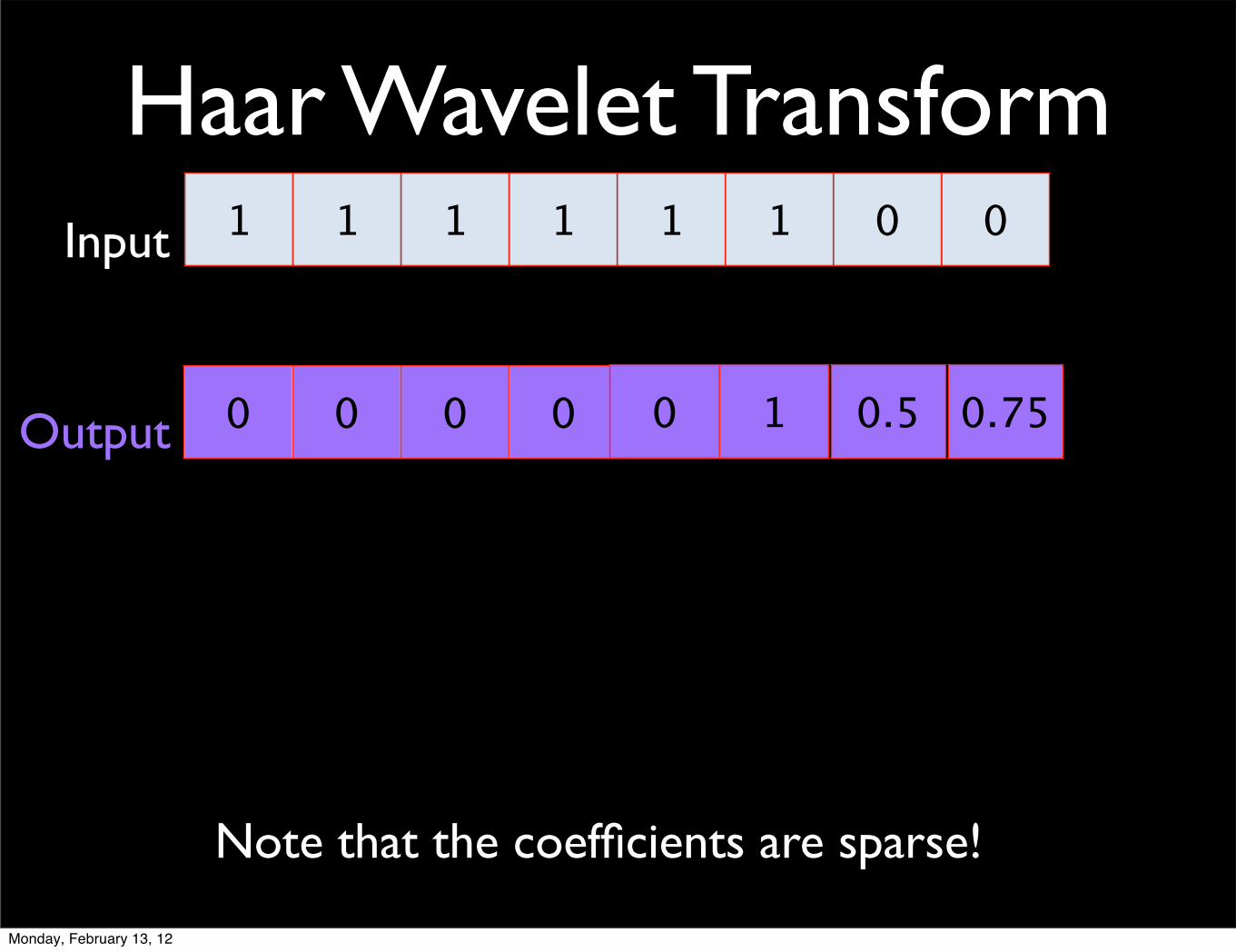
Haar Wavelet Transform1 1 1 1 1 1 0 0
0 0 0 0 0 1 0.5 0.75
Input
Output
Note that the coefficients are sparse!
Monday, February 13, 12

Haar Wavelet Transform1 1 1 1 1 1 0 0
0 0 0 0 0 1 0.5 0.75
1.03 0.94 1.00 0.95 1.04 0.98 0.00 0.02NoisyInput
0.09 0.05 0.06 -0.02 0.01 1.00 0.47 0.745Noisy
Output
The coefficients are no longer sparse!
Input
Output
Monday, February 13, 12

Wavelet Shrinkage
• For every image patch,
• Perform 2D Haar wavelet transform.
• Perform a soft thresholding:
• Pull each coefficient towards zero(by some amount Δ.)
• The patch is now more “natural”
• Invert transform to recover patch.
Monday, February 13, 12

Wavelet Shrinkage
Huh?Partitioning the image creates artifacts.
Process 8x8 patches
Monday, February 13, 12

Wavelet Shrinkage
Process all (overlapping) patches and blend them.Monday, February 13, 12

Summary
• Non-Local Means
• Exploit the inter-patch correlations.
• Wavelet Shrinkage
• Exploit the intra-patch correlations.
• Can we perhaps do both?
Monday, February 13, 12

BM3DDabov et al., 2006 (IEEE TIP)
• “Block-Matching 3D”
• Perform wavelet thresholding.
• Also combine multiple patches.
• Widely recognized as the state-of-the-art denoising technique.
Monday, February 13, 12

BM3DDabov et al., 2006 (IEEE TIP)
• Step 1. For each patch, find similar patches.
Monday, February 13, 12

BM3DDabov et al., 2006 (IEEE TIP)
• Step 2. Group the similar patches into a stack.
Monday, February 13, 12

BM3DDabov et al., 2006 (IEEE TIP)
• Step 3. Perform a 3D Haar wavelet transform.
Monday, February 13, 12

BM3DDabov et al., 2006 (IEEE TIP)
• Step 4. Apply shrinkage (or hard thresholding.)
Monday, February 13, 12
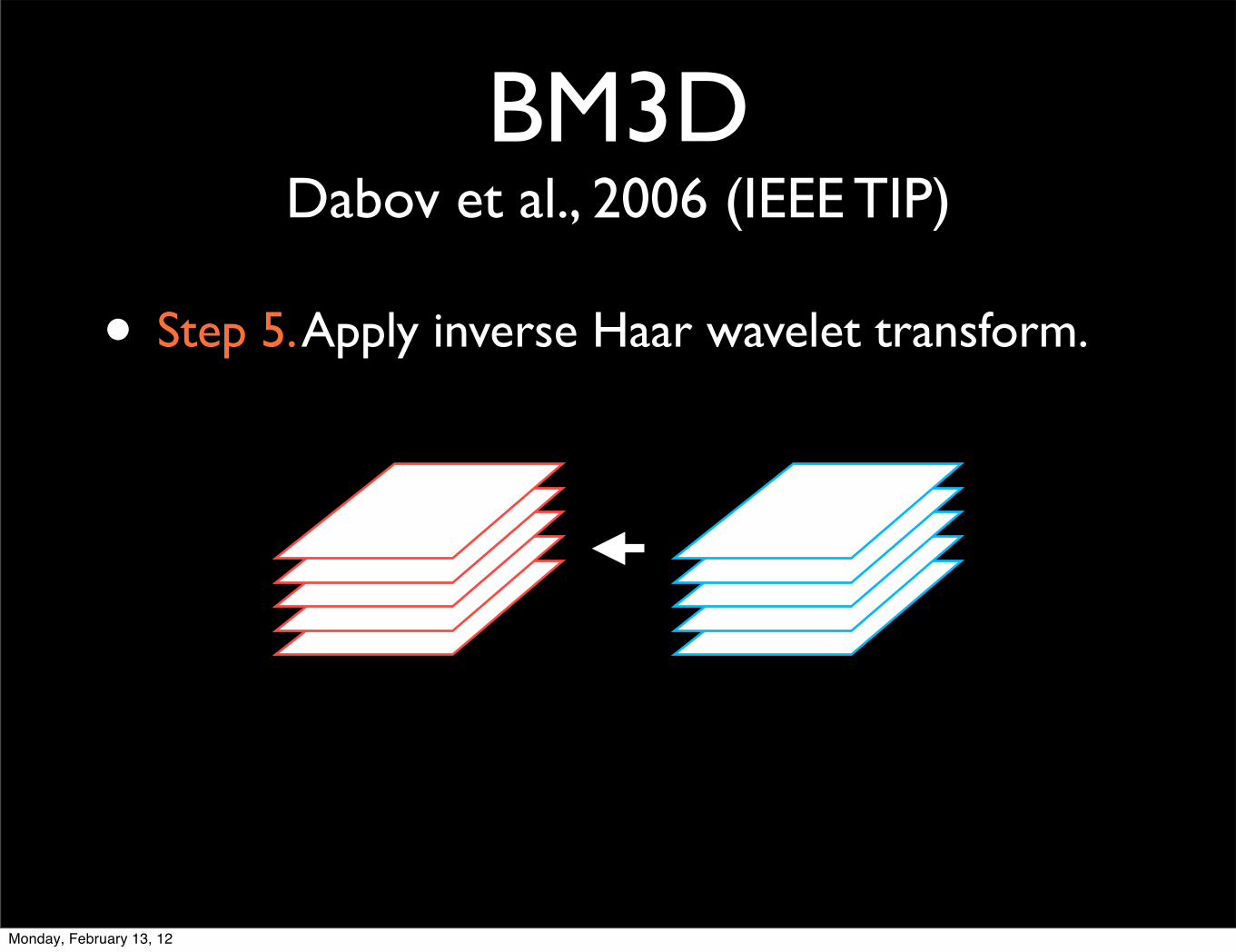
BM3DDabov et al., 2006 (IEEE TIP)
• Step 5. Apply inverse Haar wavelet transform.
Monday, February 13, 12

BM3DDabov et al., 2006 (IEEE TIP)
• Step 6. Combine the patches to form image*.
Each patch is a given weight inversely proportional to the # of nonzero entries in
wavelet domain.
Monday, February 13, 12

BM3DDabov et al., 2006 (IEEE TIP)
• Step 6. (Optional) Do it again.
Instead of thresholding, apply Wiener filter.(Attenuate each coefficient by some scale factor.)
Monday, February 13, 12

BM3DDabov et al., 2006 (IEEE TIP)
Monday, February 13, 12

BM3DDabov et al., 2006 (IEEE TIP)
Works even with really bad noise
Monday, February 13, 12

Summary
• Non-Local Means
• Exploit the inter-patch correlations.
• Wavelet Shrinkage
• Exploit the intra-patch correlations.
• BM3D
• Exploit both.
Monday, February 13, 12

Parting Thoughts
• In computational photography, we are not limited to taking a single photograph and denoising it!
• Flash-no-flash pair denoising
• Blurry-noisy pair denoising
• Stack denoising
• ...
Monday, February 13, 12

Parting Thoughts
• The ideas here can be applied elsewhere.
• Deblurring
• Sharpening
• Super-resolution
• ...
Monday, February 13, 12

Filler Slide
• How would you denoise video using one of these algorithms?
• How would you denoise a 3D mesh using one of these algorithms?
Monday, February 13, 12

Questions?
Monday, February 13, 12

Reminder• Term project proposal
• Due Wednesday
• Proposal presentation
• Next Wednesday
• Send us your slides (Keynote, PowerPoint, etc)
• 4 minutes per group
• Assignment #2 grading
• Sign up at Rm. 360.
Monday, February 13, 12