computation of quasi-periodic tori a thesis by · computation of quasi-periodic tori in the...
TRANSCRIPT

COMPUTATION OF QUASI-PERIODIC TORI
IN THE CIRCULAR RESTRICTED THREE-BODY PROBLEM
A Thesis
Submitted to the Faculty
of
Purdue University
by
Zubin Philip Olikara
In Partial Fulfillment of the
Requirements for the Degree
of
Master of Science in Aeronautics and Astronautics
August 2010
Purdue University
West Lafayette, Indiana

ii
“And I urge you to please notice when you are happy,
and exclaim or murmur or think at some point,
‘If this isn’t nice, I don’t know what is.’ ”
–Kurt Vonnegut, Jr.

iii
ACKNOWLEDGMENTS
I am truly grateful to my advisor, Professor Kathleen Howell, for her guidance during
my time at Purdue University. I am very fortunate that she believed in me early
on in my studies here. The courses she taught were some of the most enjoyable I
have taken, and the excitement she conveyed was one of my primary motivations for
pursuing research in astrodynamics. She has also tirelessly edited my work. This
thesis is a product of her careful revisions.
I appreciate the contributions of my committee members, Professors Melvin Leok
and Anil Bajaj, both of whose courses prepared me to embark on this research. I have
had many enlightening conversations with Prof. Leok, and he always has countless
ideas and suggestions. I am also grateful for him hosting my visit to the University of
California, San Diego. It was during Prof. Bajaj’s course on bifurcations and chaos
that I first became interested in quasi-periodic motions. I had no idea at the time
that the class project he suggested would lead me to my thesis research topic.
It has been a pleasure to work with the current and former members of our research
group. When I first joined, Chris Patterson was always there to answer my questions.
Dan Grebow played an important part in helping me develop as a researcher, and
it was a privilege to work with him on my first conference paper. In addition, I
have learned a great deal from my discussions with Marty Ozimek and all the group
members. I look forward to working with you all in the future. I would also like to
thank Masaki Kakoi for his constant friendship and support.
I have been very fortunate to receive financial assistance during the course of my
studies. Purdue University and the School of Aeronautics and Astronautics gener-
ously supported me throughout my undergraduate studies as well as during my first
year of graduate school with the Charles C. Chappelle Fellowship. I am also grate-
ful for continued funding from the National Science Foundation Graduate Research

iv
Fellowship Program, which has greatly simplified my time as a student.
This work would not have been possible without the help of everyone else in my
life. My parents have wholeheartedly been there for me at every step. Thanks for
everything, Dad and Mom. I am also fortunate to have a great sister, Sonia, who
has supported me since the start. Finally, I would like to thank Eric Brandner, Tyler
Lulich, and Loral O’Hara for being such great friends, and all the people I have met
at Purdue for making my time here so memorable.

v
TABLE OF CONTENTS
Page
LIST OF TABLES . . . . . . . . . . . . . . . . . . . . . . . . . . . . . . . . . vii
LIST OF FIGURES . . . . . . . . . . . . . . . . . . . . . . . . . . . . . . . . viii
ABSTRACT . . . . . . . . . . . . . . . . . . . . . . . . . . . . . . . . . . . . ix
1 INTRODUCTION . . . . . . . . . . . . . . . . . . . . . . . . . . . . . . . 1
1.1 Previous contributions . . . . . . . . . . . . . . . . . . . . . . . . . . 2
1.1.1 Historical development . . . . . . . . . . . . . . . . . . . . . . 2
1.1.2 Computational tools . . . . . . . . . . . . . . . . . . . . . . . 4
1.2 Present work . . . . . . . . . . . . . . . . . . . . . . . . . . . . . . . 5
2 BACKGROUND: CIRCULAR RESTRICTED THREE-BODY PROBLEM 8
2.1 Problem definition . . . . . . . . . . . . . . . . . . . . . . . . . . . . 8
2.1.1 Assumptions . . . . . . . . . . . . . . . . . . . . . . . . . . . . 9
2.1.2 Nondimensionalization . . . . . . . . . . . . . . . . . . . . . . 10
2.1.3 Rotating reference frame . . . . . . . . . . . . . . . . . . . . . 12
2.2 Equations of motion . . . . . . . . . . . . . . . . . . . . . . . . . . . 14
2.2.1 Lagrangian formulation . . . . . . . . . . . . . . . . . . . . . . 14
2.2.2 Hamiltonian formulation . . . . . . . . . . . . . . . . . . . . . 15
2.2.3 Jacobi constant . . . . . . . . . . . . . . . . . . . . . . . . . . 17
2.3 Libration points . . . . . . . . . . . . . . . . . . . . . . . . . . . . . . 18
3 BACKGROUND: DYNAMICAL SYSTEMS THEORY . . . . . . . . . . . 20
3.1 Continuous flows and equilibrium points . . . . . . . . . . . . . . . . 20
3.1.1 Linear flows . . . . . . . . . . . . . . . . . . . . . . . . . . . . 21
3.1.2 Nonlinear flows . . . . . . . . . . . . . . . . . . . . . . . . . . 24
3.2 Discrete maps and periodic orbits . . . . . . . . . . . . . . . . . . . . 26
3.2.1 Representing a flow as a map . . . . . . . . . . . . . . . . . . 27
vi
Page
3.2.2 Linear and nonlinear maps . . . . . . . . . . . . . . . . . . . . 28
3.2.3 Families of periodic orbits . . . . . . . . . . . . . . . . . . . . 30
3.2.4 Bifurcations of periodic orbits . . . . . . . . . . . . . . . . . . 32
3.3 Invariant tori . . . . . . . . . . . . . . . . . . . . . . . . . . . . . . . 32
3.3.1 Existence of families . . . . . . . . . . . . . . . . . . . . . . . 34
3.3.2 Torus frequencies . . . . . . . . . . . . . . . . . . . . . . . . . 35
4 COMPUTING QUASI-PERIODIC TORI . . . . . . . . . . . . . . . . . . 36
4.1 Invariance conditions and continuation . . . . . . . . . . . . . . . . . 36
4.1.1 Invariance PDE . . . . . . . . . . . . . . . . . . . . . . . . . . 37
4.1.2 Phase condition . . . . . . . . . . . . . . . . . . . . . . . . . . 38
4.1.3 Continuation . . . . . . . . . . . . . . . . . . . . . . . . . . . 40
4.2 Numerical implementation . . . . . . . . . . . . . . . . . . . . . . . . 41
4.2.1 Discretization scheme . . . . . . . . . . . . . . . . . . . . . . . 41
4.2.2 Solution approach . . . . . . . . . . . . . . . . . . . . . . . . . 42
4.2.3 Regularization . . . . . . . . . . . . . . . . . . . . . . . . . . . 45
4.3 Initialization of tori . . . . . . . . . . . . . . . . . . . . . . . . . . . . 46
4.4 Computational scheme . . . . . . . . . . . . . . . . . . . . . . . . . . 48
5 FAMILIES OF TORI IN THE EARTH-MOON CR3BP . . . . . . . . . . 51
5.1 Libration points . . . . . . . . . . . . . . . . . . . . . . . . . . . . . . 51
5.2 Periodic orbits . . . . . . . . . . . . . . . . . . . . . . . . . . . . . . . 53
5.3 Quasi-periodic tori . . . . . . . . . . . . . . . . . . . . . . . . . . . . 56
6 SUMMARY AND RECOMMENDATIONS . . . . . . . . . . . . . . . . . 64
6.1 Summary . . . . . . . . . . . . . . . . . . . . . . . . . . . . . . . . . 64
6.2 Recommendations . . . . . . . . . . . . . . . . . . . . . . . . . . . . . 65
LIST OF REFERENCES . . . . . . . . . . . . . . . . . . . . . . . . . . . . . 67

vii
LIST OF TABLES
Table Page
2.1 Characteristic quantities in sample CR3BP systems . . . . . . . . . . . . 11
5.1 Linear stability of libration points . . . . . . . . . . . . . . . . . . . . . . 52
viii
LIST OF FIGURES
Figure Page
2.1 Reference frames in plane of primary motion . . . . . . . . . . . . . . . . 12
2.2 Libration points in rotating frame . . . . . . . . . . . . . . . . . . . . . . 19
3.1 Iterations of Poincare map . . . . . . . . . . . . . . . . . . . . . . . . . . 28
3.2 Family of periodic solutions . . . . . . . . . . . . . . . . . . . . . . . . . 31
3.3 Diffeomorphism from standard torus to quasi-periodic torus . . . . . . . 34
3.4 Two-parameter family of two-dimensional tori . . . . . . . . . . . . . . . 35
4.1 Pseudo-arclength continuation . . . . . . . . . . . . . . . . . . . . . . . . 41
4.2 Example sparse structure of Jacobian . . . . . . . . . . . . . . . . . . . . 44
4.3 Eigenvector components around halo orbit . . . . . . . . . . . . . . . . . 48
4.4 Computational approach . . . . . . . . . . . . . . . . . . . . . . . . . . . 49
4.5 Steps for Lissajous orbit computation . . . . . . . . . . . . . . . . . . . . 50
4.6 Steps for quasi-halo orbit computation . . . . . . . . . . . . . . . . . . . 50
5.1 L1 Lyapunov family . . . . . . . . . . . . . . . . . . . . . . . . . . . . . 54
5.2 L2 Lyapunov family . . . . . . . . . . . . . . . . . . . . . . . . . . . . . 54
5.3 L1 vertical family . . . . . . . . . . . . . . . . . . . . . . . . . . . . . . . 54
5.4 L2 vertical family . . . . . . . . . . . . . . . . . . . . . . . . . . . . . . . 54
5.5 L1 northern halo family . . . . . . . . . . . . . . . . . . . . . . . . . . . 55
5.6 L2 northern halo family . . . . . . . . . . . . . . . . . . . . . . . . . . . 55
5.7 L4 northern W -orbit family . . . . . . . . . . . . . . . . . . . . . . . . . 56
5.8 Family of Earth-Moon L1 Lissajous tori (C = 3.179) . . . . . . . . . . . 58
5.9 Family of Earth-Moon L2 quasi-halo tori (C = 3.132) . . . . . . . . . . . 59
5.10 Family of Earth-Moon L2 quasi-halo tori (C = 3.038) . . . . . . . . . . . 61
5.11 Family of Earth-Moon L4 quasi-periodic tori (C = 2.012) . . . . . . . . . 62
5.12 Quasi-periodic torus and orbit about Earth-Moon L4 point . . . . . . . . 63

ix
ABSTRACT
Olikara, Zubin Philip. M.S.A.A., Purdue University, August 2010. Computation ofQuasi-Periodic Tori in the Circular Restricted Three-Body Problem. Major Professor:Kathleen C. Howell.
Quasi-periodic orbits lying on invariant tori in the circular restricted three-body
problem offer a broad range of mission design possibilities, but their computation
is more complex than that of periodic orbits. A preliminary framework for directly
computing two-dimensional invariant tori is presented including a natural parame-
terization and a continuation scheme. The approach is based on a scheme designed
for generic dynamical systems. Modifications are included to account for the special
family structure in the circular restricted three-body problem. A discretized partial
differential equation is solved along with constraint equations to compute members
of the family and their associated frequencies. The continuation process is initialized
from a linear estimate of a quasi-periodic torus. A regularization scheme is included
for computing invariant tori that pass close to a primary body. A method to generate
a quasi-periodic trajectory lying on the surface of the invariant torus is also presented.
The numerical methodology is demonstrated by generating families of quasi-periodic
tori with fixed Jacobi constant values that emanate from periodic orbits in the vicinity
of the Earth-Moon libration points.
1
CHAPTER 1
INTRODUCTION
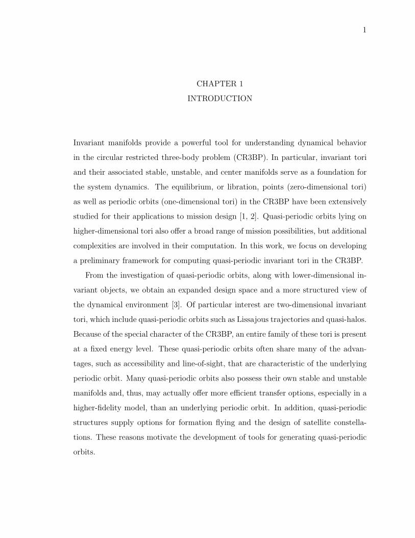
Invariant manifolds provide a powerful tool for understanding dynamical behavior
in the circular restricted three-body problem (CR3BP). In particular, invariant tori
and their associated stable, unstable, and center manifolds serve as a foundation for
the system dynamics. The equilibrium, or libration, points (zero-dimensional tori)
as well as periodic orbits (one-dimensional tori) in the CR3BP have been extensively
studied for their applications to mission design [1, 2]. Quasi-periodic orbits lying on
higher-dimensional tori also offer a broad range of mission possibilities, but additional
complexities are involved in their computation. In this work, we focus on developing
a preliminary framework for computing quasi-periodic invariant tori in the CR3BP.
From the investigation of quasi-periodic orbits, along with lower-dimensional in-
variant objects, we obtain an expanded design space and a more structured view of
the dynamical environment [3]. Of particular interest are two-dimensional invariant
tori, which include quasi-periodic orbits such as Lissajous trajectories and quasi-halos.
Because of the special character of the CR3BP, an entire family of these tori is present
at a fixed energy level. These quasi-periodic orbits often share many of the advan-
tages, such as accessibility and line-of-sight, that are characteristic of the underlying
periodic orbit. Many quasi-periodic orbits also possess their own stable and unstable
manifolds and, thus, may actually offer more efficient transfer options, especially in a
higher-fidelity model, than an underlying periodic orbit. In addition, quasi-periodic
structures supply options for formation flying and the design of satellite constella-
tions. These reasons motivate the development of tools for generating quasi-periodic
orbits.

2
1.1 PREVIOUS CONTRIBUTIONS
The three-body problem has played a fundamental role in the development of the
theory of dynamical systems. The study of the motion of three bodies, subject to their
mutual gravitational attraction, originated with Newton and his theory of gravitation.
As opposed to the two-body problem, whose solution was available at the end of the
seventeenth century, the analysis of the three-body problem proved to be much more
challenging. It was not until the advent of the modern computer that some of the
problem’s more complex behavior could be understood.
1.1.1 Historical development
Beginning in the 1700s, an important philosophical question emerged that pertained
to the stability of the solar system and the so-called n-body problem. Since many of
the problem’s complexities were present for the case n = 3, the three-body problem
was of particular interest to the mathematical and astronomical communities. In
addition, analysis of the three-body problem offered practical applications. For ex-
ample, determining the location of the Moon, as influenced by the Sun and the Earth,
was a focus due to the Moon’s use in navigation. Many of the top mathematicians
and astronomers contributed to the study of the problem, and at the turn of the
twentieth century, over 800 memoirs had been written on the subject [4]. Much of the
early work was analytical in nature, but it eventually became clear that a closed-form
solution, in terms of elementary functions, was not possible. A solution was finally
provided in Sundman’s 1912 memoir [5], but the convergence of the infinite series was
much too slow for any practical use.
Relatively early in the study of the three-body problem, Euler observed that a sim-
plified version, one that retained many of the problem’s interesting qualities, could
also be analyzed. In his 1767 work [6], he first presented the circular restricted-three
body problem (sometimes simply denoted the restricted three-body problem), where
one body has infinitesimal mass and the two primary bodies travel in circular orbits

3
about their barycenter. He also introduced the standard rotating frame of reference.
The CR3BP was useful, for example, to approximate the motion of the much-less-
massive Moon under the influence of the Sun and the Earth, which moves in a nearly
circular orbit. Euler demonstrated that there are three possible locations on the line
connecting the two primary bodies at which a particle will remain fixed. These equi-
librium points in the rotating reference frame are the collinear libration points, labeled
L1, L2, and L3. Soon after, in 1772, Lagrange proved the existence of two additional
equilibrium points, the triangular libration points L4 and L5, which lie in the primary
bodies’ plane of motion and are located at the vertices of equilateral triangles. The
other two vertices are the primary positions. Jacobi [7] then demonstrated that the
CR3BP admits an integral of motion, often termed the Jacobi constant.
A major shift in the analysis of the three-body problem began with the American
astronomer Hill’s search for periodic solutions [8]. His work had profound influence
on the French mathematician Poincare, who recognized the importance of periodic
orbits in understanding the qualitative dynamics of a system such as the CR3BP that
lacked a closed-form solution. Poincare’s celebrated 1890 paper [9] demonstrated the
role of objects such as periodic orbits in forming a framework for a system’s dynam-
ical behavior. He expanded on these ideas in his renowned memoir Les Methodes
Nouvelles de la Mecanique Celeste [10]. Through the course of this study, Poincare
discovered what is now known as chaotic motion. Poincare’s work formed the foun-
dation of modern-day dynamical systems theory and greatly influenced Birkhoff [11],
who introduced the study of general dynamical systems, independent of a particular
system. Many new lines of research were exposed by Poincare, including the study
of quasi-periodic motion that was conducted by Kolmogorov, Arnold, and Moser in
the 1950s and 1960s leading to the formation of the influential KAM theory. A de-
tailed overview of the history of the three-body problem and particularly the role of
Poincare is available in Barrow-Green [12].

4
1.1.2 Computational tools
Since a closed-form solution to the CR3BP is unavailable, researchers sought to com-
pute approximate trajectories using both analytical and numerical tools. After three
years of computation, Darwin [13] completed the first methodical, numerical search
for in-plane periodic orbits in 1897. Plummer [14, 15] investigated similar orbits via
analytical investigations, and Moulton [16], in his 1920 work, expanded this search
using a variety of approaches to include out-of-plane orbits in the CR3BP. Later,
with the dawn of the space age and the interest in engineering applications, many
of the studies began to focus on the Earth-Moon translunar L2 libration point. In
1968, Farquhar [17] developed approximations of out-of-plane periodic orbits about
the translunar point. Along with Kamel [18], he expanded these results in 1973
via the Poincare-Lindstedt method to include third-order approximations of quasi-
periodic orbits about this libration point. Two years later, Richardson and Cary [19]
generated a third-order approximation of quasi-periodic motion in the vicinity of the
Sun-Earth L1 and L2 points using the method of multiple time scales and including
eccentric effects.
With the dramatic growth of computing resources since the 1960s, many re-
searchers have also adapted analytical and numerical methods to analyze dynam-
ical systems on a computer. Since the computation of quasi-periodic trajectories
and the invariant tori upon which they lie is an important capability, various strate-
gies were developed for general dynamical systems. To date, however, only some
of these computational approaches have been applied to problems in astrodynamics.
For Hamiltonian systems such as the CR3BP, semi-analytical methods are available
for computing invariant tori. Two such semi-analytical methods are center manifold
reduction [20] and the Poincare-Lindstedt method [21]. These local methods offer
a thorough view of the dynamics in the vicinity of the libration points, but both
are limited by their regions of convergence. Specialized algebraic manipulators are
often required as well, which can create difficulties in the implementation. Purely
numerical methods offer an alternate approach to overcome these limitations. Such

5
numerical algorithms typically focus on either the invariant curves of a map or the
invariant tori of the flow in a vector field. For example, Jorba and Olmedo [22, 23]
used a Fourier series to describe an invariant curve representing the intersection of an
invariant torus with a Poincare section in a perturbed CR3BP. Gomez and Mondelo
[24] developed the Fourier expansion associated with a curve lying on the surface of
a two-dimensional torus in the CR3BP, and used an invariance condition based on
multiple shooting.
1.2 PRESENT WORK
The focus of this current analysis is also the direct computation of two-dimensional
invariant tori, but the approach here can be generalized to higher-dimensional tori
without much difficulty. To avoid the dependence on a surface of section, we present
a computational scheme based on a method developed by Schilder, Osinga, and Vogt
[25] in 2005. This approach is designed for generic dynamical systems, but can be
applied to trajectory design with some modifications relevant to systems with special
structure such as the CR3BP. In particular, for a generic dynamical system to possess
a family of two-dimensional tori, at least one system parameter is required. For
a Hamiltonian system, this family can exist without any external parameters. We
develop a scheme where additional, “artificial” parameters are incorporated in the
CR3BP such that a generic method can be applied but the dynamics are unaffected.
In contrast to the work of Gomez and Mondelo, computation of tori in the analysis
here incorporates an invariance partial differential equation (PDE). This strategy
enforces the CR3BP vector field on the quasi-periodic torus to be everywhere tangent.
Central differencing of this PDE yields a system of equations that is straightforward
to solve using a Newton method along with a sparse linear system solver. Although
this process results in a less precise approximation of the invariant torus, no forward
integration is necessary, as opposed to a method based on multiple shooting. Both
computational approaches produce a natural, global parameterization of the torus
(i.e., any state on the torus can be identified by two angles, θ1, θ2), but a more
6
efficient evaluation of the corresponding state is available with the invariance PDE
method. The availability of a multiple-parameter spline approximation allows quasi-
periodic trajectories on the surface of the invariant torus to quickly be determined
from various starting points. If greater accuracy is required, an approximate quasi-
periodic trajectory is a suitable input to a corrections process. Once a design is
completed in the CR3BP, the trajectory can be transitioned to a higher-fidelity model.
An additional benefit of the current invariance PDE approach is that continua-
tion proceeds in an intuitive manner without the introduction of constraints on the
components of a Fourier expansion. Since two-dimensional quasi-periodic tori in the
CR3BP exist in two-parameter families, there are a variety of options for their con-
tinuation. The family can first be reduced to a single parameter by fixing the ratio
of basic frequencies, ω2/ω1 (where ω1 = θ1, ω2 = θ2), or the Jacobi constant, C, in
the CR3BP. We select the latter option for the current study, and this is particularly
applicable for mission design where the goal is often a set of orbits that exist at a
certain energy level. Pseudo-arclength continuation is then applied to generate con-
stant energy families of quasi-periodic tori, such as a family of Lissajous trajectories
in the Earth-Moon system originating from a planar Lyapunov periodic orbit and
terminating with a vertical periodic orbit at the corresponding energy level. We also
introduce a regularization scheme to compute quasi-periodic tori that pass close to
one of the primary bodies.
This thesis is organized in the following manner:
Chapter 2: In this chapter, we present the assumptions upon which the CR3BP sys-
tem is based. We establish the rotating reference frame and derive the nondimen-
sional equations of motion. The Jacobi constant, the system’s integral of motion,
is also determined. In addition, we explain the locations of the five libration
points.
Chapter 3: We discuss concepts from dynamical systems theory that are applicable to
the later analysis. We introduce the study of invariant tori (equilibrium points, pe-

7
riodic orbits, and quasi-periodic tori) and the behavior in their vicinity. Attention
is given to the types of families in which these invariant objects are associated.
Chapter 4: We present the methodology for computing quasi-periodic invariant tori.
We include an initialization, continuation, and discretization scheme. A regular-
ization method is introduced to compute tori near singularities in the CR3BP. We
also discuss the generation of quasi-periodic trajectories lying on the surface of an
invariant torus.
Chapter 5: To illustrate the approach, we investigate invariant tori in the Earth-
Moon system. We consider motion near the libration points and periodic orbits,
and we demonstrate the effectiveness of the methodology by computing families
of two-dimensional quasi-periodic tori.
Chapter 6: We summarize our results and present general conclusions. In addition,
we discuss some areas for further study.
8
CHAPTER 2
BACKGROUND: CIRCULAR RESTRICTED THREE-BODY PROBLEM
In the current study, we consider motion in the circular restricted three-body problem.
This problem represents a system useful for modeling regimes where two astronomical
bodies appreciably influence the motion of a much-less-massive third body. Examples
include spacecraft motion in the Earth-Moon and Sun-Earth systems. In this chapter,
we present the problem’s basic assumptions along with the characteristic quantities,
which are used for nondimensionalization, and the rotating frame of reference. The
equations of motion are derived using both Lagrangian and Hamiltonian formulations,
which readily provide an integral of motion. In addition, the five equilibrium solutions,
also denoted libration points, are determined. Extensive introductions to the circular
restricted three-body problem are available in Szebehely [26] and Roy [27].
2.1 PROBLEM DEFINITION
The dynamical behavior of three bodies, modeled as point masses subject to their
mutual attraction, is governed by the universal law of gravitation. From Newton’s
second law of motion, we represent the dynamics of each body by the vector equation
mir′′i = −
3∑j=1, j 6=i
Gmimj
‖rij‖3 rij for i = 1, 2, 3, (2.1)
where G denotes the gravitational constant. The i-th body possesses mass mi, and its
position is represented by the vector ri ∈ R3 with respect to the inertially-fixed system
barycenter. To simplify the notation, we define the relative position vector rij :=
ri − rj. The prime symbol represents differentiation in an inertial reference frame

9
with respect to time. We use boldface to identify vectors, which, unless otherwise
noted, are assumed to be column vectors.
Since the position ri of each body depends on the positions of the other two bodies,
we would need to solve three vector second-order differential equations (2.1) simulta-
neously to determine the motion of all three bodies. However, it was demonstrated
in the late nineteenth century that this eighteen-dimensional system is non-integrable
[12], and therefore, a closed-form solution in terms of elementary functions is not
available. All solutions of the general three-body problem, such as Sundman’s [5],
necessarily depend on infinite series.
2.1.1 Assumptions
It is common to make simplifying assumptions for the problem to become more
tractable. Particularly, we would like to reduce the dimension of the system. We
accomplish this by first assuming that the mass of the third body is negligible com-
pared to the other two bodies, that is, m1,m2 � m3. Under this assumption, the
problem is labeled the restricted three-body problem. Without loss of generality, we
select the first primary body to be more massive than the second, m1 ≥ m2. Since
the third body does not influence the motion of the two primaries, their motion can
be viewed independently as a two-body problem, which is known to have a conic
solution. Defining m∗ := m1 + m2 and l∗ to be the primaries’ semi-major axis, their
mean motion (the mean angular rate of the two bodies) is
n =
(Gm∗
l∗ 3
)1/2
. (2.2)
An overview of motion in the two-body problem is available in Prussing [28].
By assuming negligible mass of the third body, we are also able to consider the
equation of motion (2.1) for i = 3 separately from the motion of the primaries (i =
1, 2), whose positions r1 and r2 are known from the conic solution. The gravitational
force from equation (2.1) acting on the third body can be derived from its potential

10
energy,
V = −Gm1m3
‖r13‖− Gm2m3
‖r23‖, (2.3)
which is a scalar function of the position vector r3 through the relative position
vectors. In addition, the third body’s kinetic energy is determined by the scalar
function
T =1
2m3 ‖r′3‖
2, (2.4)
which depends on the velocity vector r′3.
We can further assume that the primaries travel in circular orbits, a special case
of conic motion. This system is known as the circular restricted three-body prob-
lem (CR3BP). Since the orbits are circular, the primaries are a constant distance l∗
apart and rotate at a constant rate n about their barycenter, which is equivalent to
the system barycenter due to the third body’s negligible mass. The circular-orbit
assumption will also allow us to define a reference frame such that the third-body
vector equation of motion does not depend explicitly on time, effectively reducing the
system’s dimension by one.
2.1.2 Nondimensionalization
To reduce the CR3BP to its most relevant aspects, we choose to nondimensionalize the
quantities in the problem. We select the characteristic length to be l∗, the distance
between the primaries, and define the distances d := ‖r13‖ /l∗ and r := ‖r23‖ /l∗.
The characteristic time is selected to be t∗ := 1/n = (l∗ 3/Gm∗)1/2 in order to yield a
nondimensional mean motion value n = 1. Thus, the primaries complete one revolu-
tion in 2π nondimensional time units, which also allows us to view the nondimensional
time t as an angle (in radians) locating the primaries in their circular orbits.
Associated with the third body, the potential energy from equation (2.3) and
kinetic energy from equation (2.4) are nondimensionalized using the constant factor
E∗ := m3
(l∗
t∗
)2
= m3Gm∗
l∗, (2.5)
11
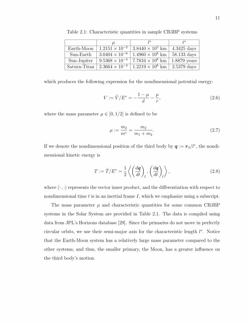
Table 2.1: Characteristic quantities in sample CR3BP systems
µ l∗ t∗
Earth-Moon 1.2151× 10⁻² 3.8440× 10⁵ km 4.3425 daysSun-Earth 3.0404× 10⁻⁶ 1.4960× 10⁸ km 58.133 days
Sun-Jupiter 9.5368× 10⁻⁴ 7.7834× 10⁸ km 1.8879 yearsSaturn-Titan 2.3664× 10⁻⁴ 1.2219× 10⁶ km 2.5379 days
which produces the following expression for the nondimensional potential energy:
V := V /E∗ = −1− µd− µ
r, (2.6)
where the mass parameter µ ∈ [0, 1/2] is defined to be
µ :=m2
m∗=
m2
m1 +m2
. (2.7)
If we denote the nondimensional position of the third body by q := r3/l∗, the nondi-
mensional kinetic energy is
T := T /E∗ =1
2
⟨(dq
dt
)I
,
(dq
dt
)I
⟩, (2.8)
where 〈· , ·〉 represents the vector inner product, and the differentiation with respect to
nondimensional time t is in an inertial frame I, which we emphasize using a subscript.
The mass parameter µ and characteristic quantities for some common CR3BP
systems in the Solar System are provided in Table 2.1. The data is compiled using
data from JPL’s Horizons database [29]. Since the primaries do not move in perfectly
circular orbits, we use their semi-major axis for the characteristic length l∗. Notice
that the Earth-Moon system has a relatively large mass parameter compared to the
other systems, and thus, the smaller primary, the Moon, has a greater influence on
the third body’s motion.

12
Figure 2.1: Reference frames in plane of primary motion
2.1.3 Rotating reference frame
If we consider the dynamic behavior in an inertial reference frame I, there is an
explicit dependence on time due to the motion of the two primary bodies relative
to an inertial observer. We remove this time dependence by introducing a frame R,
as seen in Figure 2.1, that rotates along with the primaries such that unit vector e1
is directed from the larger to the smaller primary. Unit vector e3 is parallel to the
primaries’ angular momentum vector and perpendicular to their plane of motion, and
e2 lies in the plane of the primaries completing the right-handed system. The origin
is located at the inertially-fixed barycenter, B, of the primaries. The orientation of
the rotating reference frame R relative to inertial frame I, which is spanned by unit
vectors i1, i2, and i3, and defined to coincide at time t = 0, also appears in Figure
2.1.
We represent the nondimensional position of the third body in the rotating frame
via the vector q := xe1 + ye2 + ze3 = (x, y, z) ∈ R3. In these coordinates, the larger
primary is located at (−µ, 0, 0) and the smaller primary at (1−µ, 0, 0). The distance
13
from the larger primary P1 to the third body is
d = ‖q + µe1‖ =((x+ µ)2 + y2 + z2
)1/2, (2.9a)
and the distance from the smaller primary P2 is
r = ‖q − (1− µ)e1‖ =((x− 1 + µ)2 + y2 + z2
)1/2, (2.9b)
which are both used in the potential function
V (q) = −1− µd− µ
r, (2.10)
from equation (2.6).
We can write the velocity (dq/dt)I of the third body relative to the inertial frame
I, which appears in the kinetic energy equation (2.8), in rotating frame coordinates
using the relation (dq
dt
)I
=
(dq
dt
)R
+ ne3 × q
= (x− y)e1 + (y + x)e2 + ze3,
(2.11)
where q := (dq/dt)R is the nondimensional velocity relative to the rotating frame R.
Recall that frame R rotates with angular velocity n = 1 relative to the frame I. If
we substitute equation (2.11) into equation (2.8), we are able to obtain the kinetic
energy,
T (q, q) =1
2
(x2 + y2 + z2 − 2xy + 2yx+ x2 + y2
), (2.12)
in terms of rotating frame coordinates.

14
2.2 EQUATIONS OF MOTION
A variety of approaches are available for deriving the equations of motions in the
CR3BP. We present both the Lagrangian and Hamiltonian formulations of the equa-
tions since they use different sets of variables, both of which offer insight into the
problem. In addition, by demonstrating that the CR3BP is a Hamiltonian system,
we are able to directly determine an integral of motion. The special structure of
Hamiltonian systems is also exploited later in the analysis.
2.2.1 Lagrangian formulation
Since the set of (generalized) coordinates q = (x, y, z), which represent the location
of the third body relative to the barycenter, are independent, and the gravitational
force is derivable from the potential function V in equation (2.10), we can use the
standard form of Lagrange’s equations for a holonomic system,
d
dt
∂L
∂q− ∂L
∂q= 0, (2.13)
where L := T − V is the Lagrangian of the system [30]. This generates a system of
three scalar second-order differential equations governing motion in the CR3BP.
x− 2y = −1− µd3
(x+ µ)− µ
r3(x− 1 + µ) + x, (2.14a)
y + 2x = −1− µd3
y − µ
r3y + y, (2.14b)
z = −1− µd3
z − µ
r3z, (2.14c)
where distances d and r are defined in equations (2.9a)–(2.9b). By introducing an
effective potential function
U(q) =1− µd
+µ
r+
1
2
(x2 + y2
), (2.15)
15
the equations of motion (2.14) can be written compactly as the equivalent first-order
system q
v
= x = f(x) =
v
∂U/∂q + 2v × e3
(2.16)
where v = (vx, vy, vz) ∈ R3 is the velocity of the third body in the rotating frame,
and x ∈ R6 denotes the complete state column vector (q,v) in terms of generalized
coordinates and velocities. Note that for partial derivatives, such as ∂U/∂q, that are
understood to be column vectors, the transpose operation is not explicitly denoted.
Also, we observe that f is infinitely differentiable over R6, excluding the primaries
where d = 0 or r = 0.
Examining equation (2.14c), we see that for any state with position and velocity
components z = z = 0, there is no out-of-plane acceleration, and the motion in
the plane of the primaries, governed by equations (2.14a)–(2.14b), can be considered
separately. By removing the out-of-plane components, the phase space of x is reduced
from six to four dimensions. This system is known as the planar circular restricted
three-body problem, though the spatial CR3BP is the focus of the current analysis.
2.2.2 Hamiltonian formulation
A system governed by Lagrange’s equations in their standard form (2.13) can be
alternatively represented in terms of Hamilton’s equations [30]. First, the generalized
momenta are defined in vector form by
(px, py, pz) = p :=∂L
∂q= (x− y, y + x, z). (2.17)
From equation (2.11) we note that the generalized momentum p is equivalent to the
velocity (dq/dt)I relative to an inertial observer. Rearranging equation (2.17), we
can represent velocity q relative to a rotating frame observer as a function of the
generalized position and momentum, (x, y, z) = q(q,p) = (px + y, py − x, pz). This

16
relationship allows us to rewrite the kinetic energy from equation (2.12) as
T (q,p) = T (p) =1
2
(p2x + p2
y + p2z
). (2.18)
Thus, we can represent the Lagrangian for the CR3BP in the form L(q,p) = T (p)−
V (q).
The Hamiltonian is defined to be
H(q,p, t) := 〈p, q〉 − L(q,p, t), (2.19)
where the generalized velocities q = q(q,p) are a function of the generalized position
and momenta. This produces the Hamiltonian in the CR3BP as
H(q,p) =1
2
(p2x + p2
y + p2z
)+ pxy − pyx−
1− µd− µ
r. (2.20)
For a system governed by equation (2.13), the equivalent form of Hamilton’s equations
is q
p
= x = f(x) =
+∂H/∂p
−∂H/∂q
, (2.21)
where x is used here to denote the complete state vector (q,p) ∈ R6 expressed in
terms of generalized coordinates and momenta. This can be written as a system of
six scalar first-order differential equations
x = px + y, (2.22a)
y = py − x, (2.22b)
z = pz, (2.22c)
px = py −1− µd3
(x+ µ)− µ
r3(x− 1 + µ), (2.22d)
py = −px −1− µd3
y − µ
r3y, (2.22e)
pz = −1− µd3
z − µ
r3z, (2.22f)

17
where distances d and r are defined in equations (2.9a)–(2.9b). As discussed earlier, it
is possible to consider the planar case independent of the out-of-plane directions, that
is, z = pz = 0, though the spatial case is our principal system of interest. As with
the Lagrangian formulation, the vector field defined by equation (2.22) is infinitely
differentiable except for singularities at the primaries.
2.2.3 Jacobi constant
If a Hamiltonian function H does not depend explicitly on time, it is an integral of
motion. This is readily apparent from the form of Hamilton’s equations (2.21),
dH
dt=∂H
∂q
dq
dt+∂H
∂p
dp
dt
=
⟨∂H
∂q,∂H
∂p
⟩+
⟨∂H
∂p,−∂H
∂q
⟩= 0.
(2.23)
Thus, equation (2.20) defines an integral of motion in the CR3BP, and its value is
constant along any trajectory. The related integral of motion C := −2H, known as
the Jacobi constant, is often used alternatively:
C(q,p) =2(1− µ)
d+
2µ
r− 2pxy + 2pyx−
(p2x + p2
y + p2z
). (2.24a)
The Jacobi constant can also be written in terms of position and velocity as
C(q,v) =2(1− µ)
d+
2µ
r+ x2 + y2 −
(v2x + v2
y + v2z
). (2.24b)
Since the Hamiltonian H = −C/2 is a function corresponding to the third body’s
energy, states at a higher energy level correspond to a lower Jacobi constant value.
We can consider the set of states (q,v) or (q,p) at a certain energy level, or
equivalently, Jacobi constant value. Since the Jacobi constant does not vary along a
trajectory, the “flow” as these states evolve will also possess the same Jacobi constant.

18
Therefore, by fixing the Jacobi constant C, the dimension of the problem is effectively
reduced by one. This concept of an invariant subspace is discussed further in the next
chapter.
2.3 LIBRATION POINTS
There are five well-known libration points, which are equilibrium solutions to the
equations of motion. Let us consider equation (2.14). If y = 0 and z = 0, equations
(2.14b)–(2.14c) are satisfied, and the restriction to the x-axis corresponds to the three
collinear libration points. From equations (2.9a)–(2.9b), we can write d = |x+ µ| =
sd(x + µ) and r = |x− 1 + µ| = sr(x − 1 + µ) where coefficients sd = ±1, sr = ±1
are selected such that d, r > 0 at the collinear libration point:
L1 : sd = +1, sr = −1 (2.25a)
L2 : sd = +1, sr = +1 (2.25b)
L3 : sd = −1, sr = −1 (2.25c)
The equilibrium solution of equation (2.14a) can then be represented by a quintic
polynomial,
x5 + c4x4 + c3x
3 + c2x2 + c1x+ c0 = 0, (2.26)
with coefficients
c0 := (sd − sr)µ3 − 3sdµ2 + 3sdµ− sd, (2.27a)
c1 := µ4 − 2µ3 + (2sd − 2sr + 1)µ2 − 4sdµ+ 2sd, (2.27b)
c2 := 4µ3 − 6µ2 + (sd − sr + 2)µ− sd, (2.27c)
c3 := 6µ2 − 6µ+ 1, (2.27d)
c4 := 4µ− 2. (2.27e)
19
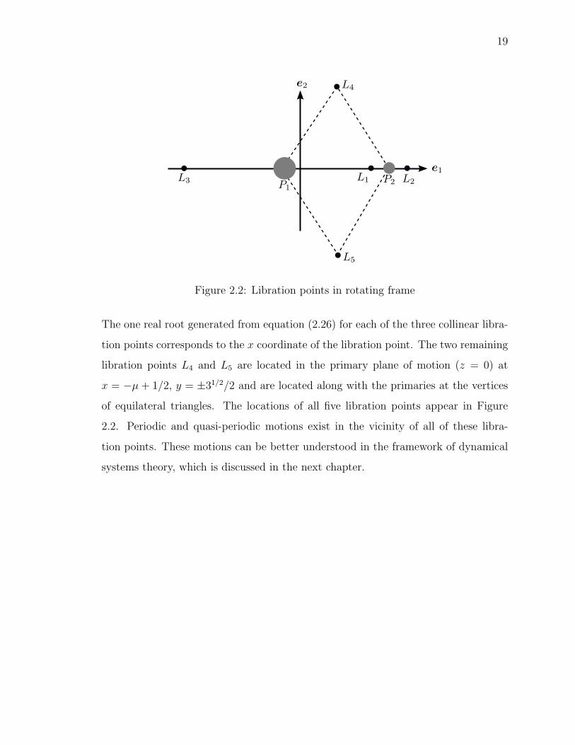
Figure 2.2: Libration points in rotating frame
The one real root generated from equation (2.26) for each of the three collinear libra-
tion points corresponds to the x coordinate of the libration point. The two remaining
libration points L4 and L5 are located in the primary plane of motion (z = 0) at
x = −µ + 1/2, y = ±31/2/2 and are located along with the primaries at the vertices
of equilateral triangles. The locations of all five libration points appear in Figure
2.2. Periodic and quasi-periodic motions exist in the vicinity of all of these libra-
tion points. These motions can be better understood in the framework of dynamical
systems theory, which is discussed in the next chapter.

20
CHAPTER 3
BACKGROUND: DYNAMICAL SYSTEMS THEORY
Dynamical behavior in a broad range of systems can be explored via the framework
of dynamical systems theory. In this chapter, we explore the basic invariant objects
(equilibrium points, periodic orbits, and invariant tori) and the behavior in their
vicinity. We begin by analyzing equilibrium points of linear and nonlinear continuous
time flows. We then discuss the view of a periodic orbit as a fixed point of a discrete
map, and present general characteristics of linear and nonlinear maps. In addition,
we investigate families of periodic orbits and their bifurcations. Finally, we consider
invariant tori and their associated families. Wiggins [31], Guckenheimer [32], and
Perko [33] offer detailed introductions to the theory of dynamical systems.
3.1 CONTINUOUS FLOWS AND EQUILIBRIUM POINTS
We can view the CR3BP equations of motion, as represented in equations (2.16) and
(2.22), generically as an autonomous ordinary differential equation in the vector form
x = f(x,λ), (3.1)
where x(t) ∈ Rn is a state vector, and f defines a differentiable vector field depending
on external parameters λ ∈ Rm. The spatial CR3BP is a six-dimensional (n = 6)
system with m = 0 external parameters, since we generally do not allow the mass
parameter µ to vary. If it is not necessary to express the parameters λ of a system
explicitly, we often write equation (3.1) simply as
x = f(x). (3.2)

21
The associated vector field leads to a corresponding flow φ mapping an initial state
x0 at time zero to the corresponding state φ(t,x0) at time t along the trajectory. The
flow is defined such that φ(0,x0) = x0, and the time derivative along the trajectory
corresponds to the vector field,
d
dtφ(t,x0) = f(φ(t,x0)). (3.3)
We will use the common notation where time t is represented using a subscript,
φt(·) := φ(t, ·).
The dynamical behavior associated with equation (3.2) can be complex for many
nonlinear systems, particularly systems with phase space dimension-n larger than two
or three. However, there may, in fact, exist lower-dimensional subspaces on which the
“interesting” dynamics occur. These subspaces form a framework for the dynamics of
the system. We approach the study of such a subspace by introducing the concept of
an invariant set, which is defined to be a set M such that any state starting in the
set flowed forward or backward in time still belongs to the set,
φt(x0) ∈M for all x0 ∈M, t ∈ R. (3.4)
If the set M possesses the structure of a manifold (roughly speaking, the vicinity of
any point can be viewed locally as a Euclidean space), then it is termed an invariant
manifold. A trivial example of an invariant manifold is the entire phase space itself.
More interesting examples include equilibrium points and periodic orbits as well as
manifolds that asymptotically approach and depart them. In addition, for a system
such as the CR3BP possessing an integral of motion, the set of states at a certain
integral (e.g., Jacobi constant) value form an invariant manifold.
3.1.1 Linear flows
The most basic solution to equation (3.2) is an equilibrium point, x (also referred
to as a fixed point). To analyze the dynamics near an equilibrium point of a vector

22
field, we first consider the linear case, which we later demonstrate can be used to
extract information about the nonlinear case. We begin by considering a linear system
governed by the differential equation
y = Ay, (3.5)
where y(t) ∈ Rn and A ∈ Rn×n is a constant, real matrix. Clearly, y(·) = 0 is an
equilibrium solution of this differential equation. For any initial condition y(0), the
solution is of the form
y(t) = eAty(0), (3.6)
where the matrix exponential is defined to be
eAt := I +At+1
2!A2t2 +
1
3!A3t3 + · · · . (3.7)
Note that this is a direct vector generalization of the solution to a scalar, linear
differential equation.
Let us consider the simple case where A has n real eigenvalues λ1, . . . , λn, and the
the associated (real) eigenvectors v1, . . . ,vn are linearly independent, which is true if
the eigenvalues are distinct. If we define the columns of matrix P :=[v1 · · · vn
]to consist of the eigenvectors, then matrix P diagonalizes matrix A,
J = P−1AP =
λ1
. . .
λn
. (3.8)
23
From the definition of the matrix exponential and noting that(PJP−1
)k= PJkP−1
for any k ≥ 0, we see that
y(t) = eP JP−1ty(0)
= P eJtP−1y(0)
=[v1e
λ1t · · · vneλnt
]P−1y(0).
(3.9)
Then, P−1 can be viewed as transforming initial condition y(0) into the eigenbasis,
and P eJt represents the flow in each of the eigendirections vi being scaled by a factor
eλit.
We can generalize these results to any real matrix A by choosing J to be in
real Jordan normal form, and then determining the (real) generalized eigenvectors
which comprise the columns of P . Details on this approach is available in Strang [34]
and Guckenheimer [32]. For the example case where A is diagonalizable, the Jordan
normal form is simply the diagonalized matrix.
This example case with real eigenvalues and independent eigenvectors suggests
that each eigenvalue determines the behavior of the flow in its corresponding eigendi-
rection. It can be demonstrated (see [31, 32]) that there are three possible motions
for each eigenvalue λi, or in other words, the spectrum of A can be grouped into three
parts corresponding to:
1. Stable motion: Re [λi] < 0. If there are ns stable eigenvalues, the corresponding
set of (real, generalized) eigenvectors form a basis for the stable subspace Es =
span{vs1, . . . ,v
sns
}.
2. Unstable motion: Re [λi] > 0. If there are nu unstable eigenvalues, the cor-
responding set of (real, generalized) eigenvectors form a basis for the unstable
subspace Eu = span{vu1 , . . . ,v
unu
}.
3. Center motion: Re [λi] = 0. If there are nc center eigenvalues, the corresponding
set of (real, generalized) eigenvectors form a basis for the center subspace Ec =
24
span{vc1, . . . ,v
cnc
}.
Note that the dimensions of the subspaces add up to the dimension of the phase
space, that is, ns + nu + nc = n. From the primary decomposition theorem [35], we
can further state that the stable, unstable, and center subspaces completely span the
phase space Rn of y,
Es ⊕ Eu ⊕ Ec = Rn, (3.10)
or equivalently, we can view state y as the sum of its projections onto the subspaces,
each of which has a certain category of motion.
3.1.2 Nonlinear flows
If we define the vector y := x − x, then the linearized flow about the equilibrium
point x of the nonlinear system in equation (3.2) is governed by
y = Df(x)y, (3.11)
where the constant matrix Df(x) := ∂f(x)/∂x. If the equilibrium point x is hyper-
bolic, we are able to apply the results from the analysis of this linear system to the
corresponding nonlinear system using the Hartman-Grobman theorem, which demon-
strates that near the equilibrium point, the flow is topologically equivalent between
the systems provided certain non-degeneracy conditions are met. This equivalency is
represented by a homeomorphism, which is a continuous map between spaces with a
continuous inverse.
Theorem 3.1 (Hartman-Grobman Theorem, from Guckenheimer [32]): If Df(x) has
no zero or purely imaginary eigenvalues, then there is a homeomorphism defined on
some neighborhood U of x in Rn locally taking orbits of the nonlinear flow φt of equa-
tion (3.2), to those of the linear flow eDf(x)t of equation (3.11). The homeomorphism
preserves the sense of orbits and can also be chosen to preserve parameterization by
time.
25
Since the Hartman-Grobman theorem requires that Df(x) possesses no eigen-
values on the imaginary axis, it applies when the center subspace is empty, Ec = ∅.
However, using the stable, unstable, and center manifold theorem, we can still obtain
results for a nonlinear system where the linearization Df(x) has any eigenvalue spec-
trum. Since we are interested in subspaces that asymptotically approach or depart
the equilibrium point, analogous to the stable and unstable subspaces of the linear
system in equation (3.5), we define the stable manifold locally as
W sloc(x) := {x ∈ U |φt(x)→ x as t→∞, φt(x) ∈ U for all t ≥ 0} , (3.12)
and the unstable manifold locally as
W uloc(x) := {x ∈ U |φt(x)→ x as t→ −∞, φt(x) ∈ U for all t ≤ 0} . (3.13)
Combining theorems from Guckenheimer [32] and Perko [33], we obtain the following
result:
Theorem 3.2 (Stable, Unstable, and Center Manifold Theorem): Suppose that equation
(3.2), x = f(x), possesses a fixed point x. Then there exist local stable, unstable, and
center manifolds W sloc(x), W u
loc(x), W cloc(x) of dimension ns, nu, nc that are tangent
to Es, Eu, Ec, respectively, at x. These manifolds are as smooth as f and invariant
under the flow φt. The stable and unstable manifolds are unique, though this is not
necessarily true for the center manifold.
This theorem confirms the existence of local stable and unstable manifolds as-
sociated with the equilibrium point of the nonlinear flow. These manifolds can be
globalized by flowing the points on the local stable manifold backwards in time,
W s(x) =⋃t≤0
φt(Wsloc(x)), (3.14)

26
and by flowing the points on the local unstable manifold forwards in time,
W u(x) =⋃t≥0
φt(Wuloc(x)). (3.15)
Any point on the stable manifold W s(x) asymptotically approaches the equilibrium
point, and any point on the unstable manifold W u(x) asymptotically departs the
equilibrium point (or equivalently, asymptotically approaches in negative time).
The center manifold W cloc(x) contains motions such as periodic and quasi-periodic
orbits, which oscillate about the fixed point, in addition to other dynamical structures
of interest. Center manifold theory concerns the reduction of a dynamical system to
the center manifold and the study of the dynamics evolving on this manifold. This
theory is discussed in Wiggins [31].
3.2 DISCRETE MAPS AND PERIODIC ORBITS
We have considered, thus far, the behavior of continuous time flows in the vicinity of
an equilibrium point. To examine the behavior near a periodic orbit of a continuous
flow, the orbit is often analyzed as the fixed point of a map, which has the form
x 7→ g(x), (3.16)
where x(k) ∈ Rn and g is a diffeomorphism, i.e., a differentiable map with a differ-
entiable inverse. We can also introduce the concept of an invariant set of a discrete
map, which is defined to be a set M such that any state in the set still belongs to the
set after any number of iterations of the map g,
gk(x0) ∈M for all x0 ∈M, k ∈ Z. (3.17)
If M has the structure of a manifold, then we label it an invariant manifold.

27
3.2.1 Representing a flow as a map
The simplest way to represent a continuous system as a discrete system is the use of
a stroboscopic map. We can define the map g := φτ in terms of the flow for some
fixed interval of time τ . If x is any point on a periodic orbit with period τ = T1,
then g(x) = φT1(x) = x, or in other words, x is a fixed point of the map g. The
linearization of the map relative to an initial state x is Dg = Dφτ = ∂φτ (x)/∂x.
The state-transition matrix Dφτ : Rn → Rn relates variations in the initial state to
variations in the final state after time τ , which is one iteration of the stroboscopic
map. Thus, Dφ0(x0) = I. In addition, by applying the chain rule, we find that
d
dtDφt(x0) =
∂f(φt(x0))
∂x0
= Df(φt(x0))Dφt(x0).
(3.18)
Therefore, the linearized map Dg(x0) = Dφτ (x0) can be computed by integrating
for time τ the matrix ordinary differential equation (3.18) along with the equation of
motion (3.2) for the continuous flow. The state-transition matrix after one period,
τ = T1, of an orbit is denoted the monodromy matrix.
A continuous flow can also be reduced to a discrete system via a Poincare map.
To construct the map, we first define a hypersurface Σ, a manifold of dimension
n− 1, that is transverse to the phase space flow. A trajectory starting from an initial
state on the hypersurface is followed until its first intersection, typically crossing
in a prescribed direction, with the hypersurface. The intersection represents the
subsequent state after an iteration of the map. This procedure discretizes the flow
and reduces the problem dimension by one. Next, since each integral of motion defines
an invariant manifold in the phase space, all the integrals of motion can be fixed to
further reduce the problem’s dimension by the number of available integrals of motion.
For example, the CR3BP has one integral of motion, the Hamiltonian from equation
(2.20) or equivalently the Jacobi constant in equation (2.24), which reduces the phase
space by an additional dimension to n − 2. Thus, the spatial CR3BP (n = 6) has a

28
Figure 3.1: Iterations of Poincare map
four-dimensional Poincare map, and the planar CR3BP (n = 4) can be investigated
via a two-dimensional Poincare map, such as the map diagrammed in Figure 3.1.
The linearization of the Poincare map follows a similar procedure to the stroboscopic
map, though special considerations are needed to account for the hypersurface and
the fixed integral of motion. While the Poincare map is not used in the current work,
details of this tool’s formulation are available in Wiggins [31] and Guckenheimer [32].
3.2.2 Linear and nonlinear maps
After a continuous time system is reduced to a discrete system, its behavior near a
fixed point can be investigated in a manner similar to the analysis of an equilibrium
point of a flow. Details are available in Wiggins [31] and Guckenheimer [32]. Let us
first consider a linear map, which we will later use in the analysis of a nonlinear map.
We begin with the system
y 7→ Ay, (3.19)
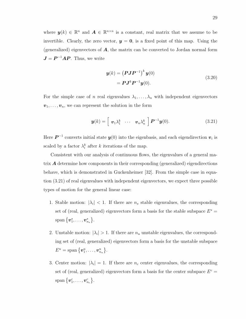
29
where y(k) ∈ Rn and A ∈ Rn×n is a constant, real matrix that we assume to be
invertible. Clearly, the zero vector, y = 0, is a fixed point of this map. Using the
(generalized) eigenvectors of A, the matrix can be converted to Jordan normal form
J = P−1AP . Thus, we write
y(k) =(PJP−1
)ky(0)
= PJkP−1y(0).(3.20)
For the simple case of n real eigenvalues λ1, . . . , λn with independent eigenvectors
v1, . . . ,vn, we can represent the solution in the form
y(k) =[v1λ
k1 · · · vnλ
kn
]P−1y(0). (3.21)
Here P−1 converts initial state y(0) into the eigenbasis, and each eigendirection vi is
scaled by a factor λki after k iterations of the map.
Consistent with our analysis of continuous flows, the eigenvalues of a general ma-
trixA determine how components in their corresponding (generalized) eigendirections
behave, which is demonstrated in Guckenheimer [32]. From the simple case in equa-
tion (3.21) of real eigenvalues with independent eigenvectors, we expect three possible
types of motion for the general linear case:
1. Stable motion: |λi| < 1. If there are ns stable eigenvalues, the corresponding
set of (real, generalized) eigenvectors form a basis for the stable subspace Es =
span{vs1, . . . ,v
sns
}.
2. Unstable motion: |λi| > 1. If there are nu unstable eigenvalues, the correspond-
ing set of (real, generalized) eigenvectors form a basis for the unstable subspace
Eu = span{vu1 , . . . ,v
unu
}.
3. Center motion: |λi| = 1. If there are nc center eigenvalues, the corresponding
set of (real, generalized) eigenvectors form a basis for the center subspace Ec =
span{vc1, . . . ,v
cnc
}.

30
For a nonlinear map, we can construct a map g, as discussed in Section 3.2.1, such
that if x is a point on a periodic orbit, it is a fixed point of the map, i.e., x = g(x).
If we define y := x− x, the linearized map near the periodic orbit takes the form
y(k) = Dg(x)y(k − 1). (3.22)
The nonlinear map in the vicinity of the fixed point x can be related to the map’s
linearization in a manner similar to the approach presented in Section 3.1.2 for con-
tinuous flows. Correspondingly, there are versions of the Hartman-Grobman theorem
and the stable, unstable, and center manifold theorem applicable to maps. These
versions are analogous to the continuous time theorems, except that the concept of
a flow φt is replaced by iterations of the discrete map g. The discrete theorems are
available in Guckenheimer [32]. These tools allow us investigate the dynamical behav-
ior in the vicinity of a periodic orbit by analyzing the behavior near the fixed point
of an associated map.
3.2.3 Families of periodic orbits
An important consideration in the study of periodic orbits is the identification of the
type of family in which they are a member. The eigenvalues of the monodromy matrix
are an important tool in this analysis. Meyer [36] proves that a periodic orbit in a
Hamiltonian system, such as the CR3BP, always possesses a monodromy matrix with
two eigenvalues, termed the trivial multipliers, that are 1. A periodic orbit in such
a system is defined to be elementary if none of the other, nontrivial multipliers are
1. It can be demonstrated that these periodic orbits lie in families governed by the
so-called cylinder theorem, which is illustrated in Figure 3.2.
Theorem 3.3 (Cylinder Theorem, from Meyer [36]): An elementary periodic orbit of a
system with an integral lies in a smooth cylinder of periodic solutions parameterized
by the integral H.
31
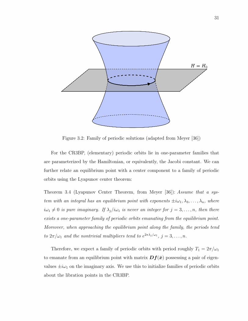
Figure 3.2: Family of periodic solutions (adapted from Meyer [36])
For the CR3BP, (elementary) periodic orbits lie in one-parameter families that
are parameterized by the Hamiltonian, or equivalently, the Jacobi constant. We can
further relate an equilibrium point with a center component to a family of periodic
orbits using the Lyapunov center theorem:
Theorem 3.4 (Lyapunov Center Theorem, from Meyer [36]): Assume that a sys-
tem with an integral has an equilibrium point with exponents ±iω1, λ3, . . . , λn, where
iω1 6= 0 is pure imaginary. If λj/iω1 is never an integer for j = 3, . . . , n, then there
exists a one-parameter family of periodic orbits emanating from the equilibrium point.
Moreover, when approaching the equilibrium point along the family, the periods tend
to 2π/ω1 and the nontrivial multipliers tend to e2πλj/ω1, j = 3, . . . , n.
Therefore, we expect a family of periodic orbits with period roughly T1 = 2π/ω1
to emanate from an equilibrium point with matrix Df(x) possessing a pair of eigen-
values ±iω1 on the imaginary axis. We use this to initialize families of periodic orbits
about the libration points in the CR3BP.

32
3.2.4 Bifurcations of periodic orbits
When applying the cylinder theorem, we assume that a periodic orbit in a family is
elementary, i.e., none of the nontrivial eigenvalues of the monodromy matrix are 1.
However, as we move between periodic orbit members of a family, the eigenvalues
change, and it is possible for this assumption to break down. The behavior at such
a breakdown is one of the focuses of bifurcation theory, and introductions to this
vast field are available in Kuznetsov [37], Wiggins [31], and Guckenheimer [32]. We
will only consider the simple branching of families, namely pitchfork and transcritical
bifurcations of periodic orbits, though many other types of bifurcations exist.
The monodromy matrix DφT1relates a variation δx of an initial state x on a pe-
riodic orbit to the variation DφT1δx after one period T1. Assuming DφT1
δx = δx,
from a linear approximation we expect the state x + δx to correspond to an initial
condition for a periodic orbit in the vicinity. Viewing the relation as an eigenvalue
problem, δx is an eigenvector of the monodromy matrix corresponding to an eigen-
value of 1. Since Hamiltonian systems have two trivial eigenvalues, the corresponding
eigenvectors span the space along the periodic orbit and along the family. If any
nontrivial eigenvalues are 1, an additional independent eigenvector, if present, would
span a space including the tangent direction of another periodic orbit family. At
this branching orbit, the periodic families intersect. We observe this periodic orbit
bifurcation behavior in the CR3BP, as is discussed later.
3.3 INVARIANT TORI
We have investigated behavior near equilibrium points (fixed points of a flow) and
periodic orbits (fixed points of a map), and we now consider how these types of funda-
mental solutions are viewed as special cases of invariant tori. In particular, analyzing
a dynamical system using invariant manifold theory often begins by identifying a “ba-
sic” invariant object (Wiggins [31] and [38]), generally a p-dimensional invariant torus
T . These include:
33
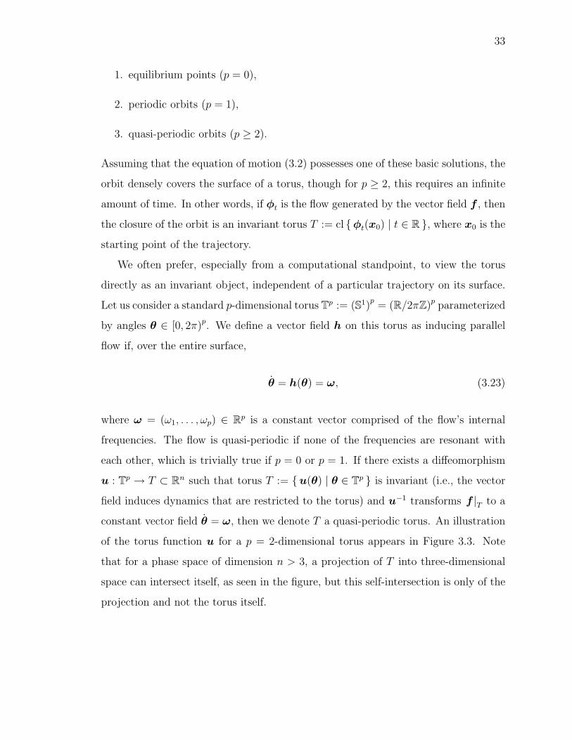
1. equilibrium points (p = 0),
2. periodic orbits (p = 1),
3. quasi-periodic orbits (p ≥ 2).
Assuming that the equation of motion (3.2) possesses one of these basic solutions, the
orbit densely covers the surface of a torus, though for p ≥ 2, this requires an infinite
amount of time. In other words, if φt is the flow generated by the vector field f , then
the closure of the orbit is an invariant torus T := cl {φt(x0) | t ∈ R }, where x0 is the
starting point of the trajectory.
We often prefer, especially from a computational standpoint, to view the torus
directly as an invariant object, independent of a particular trajectory on its surface.
Let us consider a standard p-dimensional torus Tp := (S1)p
= (R/2πZ)p parameterized
by angles θ ∈ [0, 2π)p. We define a vector field h on this torus as inducing parallel
flow if, over the entire surface,
θ = h(θ) = ω, (3.23)
where ω = (ω1, . . . , ωp) ∈ Rp is a constant vector comprised of the flow’s internal
frequencies. The flow is quasi-periodic if none of the frequencies are resonant with
each other, which is trivially true if p = 0 or p = 1. If there exists a diffeomorphism
u : Tp → T ⊂ Rn such that torus T := {u(θ) | θ ∈ Tp } is invariant (i.e., the vector
field induces dynamics that are restricted to the torus) and u−1 transforms f |T to a
constant vector field θ = ω, then we denote T a quasi-periodic torus. An illustration
of the torus function u for a p = 2-dimensional torus appears in Figure 3.3. Note
that for a phase space of dimension n > 3, a projection of T into three-dimensional
space can intersect itself, as seen in the figure, but this self-intersection is only of the
projection and not the torus itself.

34
Figure 3.3: Diffeomorphism from standard torus to quasi-periodic torus
3.3.1 Existence of families
The existence of torus solutions T to equation (3.2) is based on Kolmogorov-Arnold-
Moser (KAM) theory. We do not consider the details in the current analysis, but
some of the major results are significant for this development. An overview of KAM
theory is available in Broer [39]. For a generic system (one without structure, i.e.,
dissipative), an invariant p-dimensional torus typically lies in an m-parameter family,
where m is the number of external parameters (λ ∈ Rm). For a Hamiltonian system,
however, an invariant p-torus (for p ≤ n/2) typically lies in a (p + m)-parameter
family. Thus, p + m variables are required to identify a particular member of the
family, even though there are only m external parameters.
Assuming there exists a q-parameter family of p-tori, a Hamiltonian system will,
therefore, have p fewer external parameters than a generic system. We must incor-
porate these “missing” parameters to apply a method designed for computing quasi-
periodic tori of generic systems. The CR3BP, which is a Hamiltonian system with
m = 0 external parameters (assuming mass parameter µ is fixed), has one-parameter
families of periodic orbits and two-parameter families of two-dimensional tori, as illus-
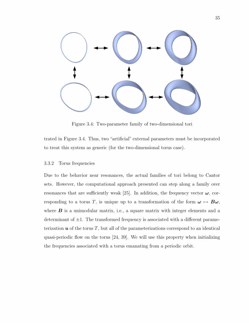
35
Figure 3.4: Two-parameter family of two-dimensional tori
trated in Figure 3.4. Thus, two “artificial” external parameters must be incorporated
to treat this system as generic (for the two-dimensional torus case).
3.3.2 Torus frequencies
Due to the behavior near resonances, the actual families of tori belong to Cantor
sets. However, the computational approach presented can step along a family over
resonances that are sufficiently weak [25]. In addition, the frequency vector ω, cor-
responding to a torus T , is unique up to a transformation of the form ω 7→ Bω,
where B is a unimodular matrix, i.e., a square matrix with integer elements and a
determinant of ±1. The transformed frequency is associated with a different parame-
terization u of the torus T , but all of the parameterizations correspond to an identical
quasi-periodic flow on the torus [24, 39]. We will use this property when initializing
the frequencies associated with a torus emanating from a periodic orbit.
36
CHAPTER 4
COMPUTING QUASI-PERIODIC TORI
In this chapter, we outline an approach for computing invariant tori in the CR3BP.
The process is applicable to tori of any dimension, but we are particularly inter-
ested in two-dimensional quasi-periodic tori and the periodic orbits from which they
emanate. The general method is based on the work of Schilder [25] with suitable
modifications for systems in which families of tori exist without any explicit external
parameters. These modifications extend the applicability of the method to systems
with an integral of motion, notably Hamiltonian systems such as the CR3BP. We
first present an invariance partial differential equation and phase condition such that
a particular torus has a unique functional representation. Then we discuss how a two-
dimensional quasi-periodic torus in a family can be isolated using a Jacobi constant
constraint and pseudo-arclength continuation. We explain the simple discretization
scheme from Schilder for solving the equations via Newton’s method and include a
bordering scheme to take into account the special structure of the system. A suitable
initial guess for a first quasi-periodic torus is provided from a periodic orbit with
a center component. We finally offer a simple method to generate a quasi-periodic
trajectory on the surface of a computed invariant torus.
4.1 INVARIANCE CONDITIONS AND CONTINUATION
As discussed in Section 3.3, a p-dimensional invariant torus T of a vector field can
be represented by the torus function u : Tp → T , which maps the standard torus
to the invariant torus, along with the associated frequency vector ω = (ω1, . . . , ωp).
In effect, u takes a location on the torus parameterized by angles θ = (θ1, . . . , θp)
to a state x ∈ Rn. By introducing an invariance PDE and a phase condition, we

37
guarantee that the torus function satisfies the vector field and that the ambiguity in
the function’s phase is removed. This approach applies to any torus of dimension
p ≥ 0, including a periodic orbit (p = 1) and a two-dimensional quasi-periodic torus
(p = 2).
4.1.1 Invariance PDE
We represent the condition on torus function u such that T is invariant, specifically
a p-dimensional quasi-periodic torus, by a partial differential equation. For motion
on the torus, the state x in equation (3.2), x = f(x), is replaced by the function
u : θ 7→ x. Applying the chain rule to the left-hand side of this equation, we obtain
the following relationship,
u =
p∑i=1
∂u
∂θi
dθidt
= f(u). (4.1)
Including equation (3.23), θ = ω, for quasi-periodic flow in the above relation, yields
the invariance PDE,p∑i=1
ωi∂u
∂θi= f(u). (4.2)
This equation guarantees that at any point θ on the torus, the vector field f is a
linear combination of the vectors {∂u/∂θ1, . . . , ∂u/∂θp}, which form a basis for the
tangent space of the torus. A solution (u,ω) to this PDE produces a quasi-periodic
invariant torus T with a natural parameterization by angles θ. We also note that
for the case of an equilibrium point (p = 0), equation (4.2) becomes the familiar
invariance relation
0 = f(u), u : T0 → Rn, (4.3)
where T0 is simply a single point. Similarly, for the periodic orbit case (p = 1), we
obtain the relationship
ω1du
dθ1
= f(u), u : T1 → Rn, (4.4)

38
where diffeomorphism u maps the standard circle T1 = S1 to a periodic orbit in Rn.
The current analysis primarily considers the two-dimensional quasi-periodic torus case
(p = 2), but we are also interested in computing families of periodic orbits from which
to initialize the two-dimensional invariant tori.
4.1.2 Phase condition
Given that the quasi-periodic torus T is defined in terms of the angles θ, the associated
phase of each remains to be constrained. If the torus function v satisfies equation
(4.2), then it is possible to define another solution u, where u(θ) := v(θ + s) with
phase shift s ∈ Tp, that corresponds to the same torus T . Given a solution u0
corresponding to a nearby torus T0 in the family, it is common to select the phase of
u such that ‖u− u0‖2 = 〈u− u0,u− u0〉 is an extremum, particularly a minimum.
We define the inner product between two torus functions v,w to be
〈v,w〉 :=1
(2π)p
ˆTp
〈v(θ),w(θ)〉 dθ, (4.5)
where 〈v(θ),w(θ)〉 =∑n
i=1 vi(θ)wi(θ) is the usual vector inner product. Schilder [25]
introduces the phase condition
⟨∂u0
∂θi,u
⟩= 0, i = 1, . . . , p, (4.6)
which guarantees that ‖u− u0‖2 is a local extremum. This condition fixes the p free
phases for the torus T and directly generalizes the integral phase condition that is
often used for periodic orbits [40].
We can prove that equation (4.6) guarantees an extremum for the case p = 1. Let
v be a torus function for a periodic orbit satisfying invariance PDE (4.2). We would
like to determine another torus function u, defined such that u(θ1) := v(θ1 + s1),
which has an extremal value for ‖u− u0‖2. This condition is equivalent to locating

39
the extremal value of the function
σ(s1) :=1
2π
ˆ 2π
0
‖v(θ1 + s1)− u0(θ1)‖2 dθ1. (4.7)
We can represent this requirement by the relationship
0 =d
ds1
σ(s1) =1
2π
ˆ 2π
0
d
ds1
‖v(θ1 + s1)− u0(θ1)‖2 dθ1
=2
2π
ˆ 2π
0
⟨v(θ1 + s1)− u0(θ1),
dv
dθ1
(θ1 + s1)
⟩dθ1.
(4.8)
If we make the substitution u(θ1) := v(θ1 + s1) and perform integration by parts
(noting that u(θ1) and u0(θ1) are 2π-periodic), we follow the steps
0 =
ˆ 2π
0
⟨u(θ1)− u0(θ1),
du
dθ1
(θ1)
⟩dθ1
= −ˆ 2π
0
⟨u(θ1),
du
dθ1
(θ1)− du0
dθ1
(θ1)
⟩dθ1
= −ˆ 2π
0
⟨u(θ1),
du
dθ1
(θ1)
⟩dθ1 +
ˆ 2π
0
⟨u(θ1),
du0
dθ1
(θ1)
⟩dθ1.
(4.9)
The first term in the last line is demonstrated to be zero using the fundamental
theorem of calculus and noting that ‖u(θ1)‖2 is 2π-periodic:
ˆ 2π
0
⟨u(θ1),
du
dθ1
(θ1)
⟩dθ1 =
1
2
ˆ 2π
0
d
dθ1
‖u(θ1)‖2 dθ1 = 0. (4.10)
Therefore, substituting equation (4.10) into equation (4.9), we obtain the phase con-
dition for a periodic orbit (p = 1),
⟨du0
dθ1
,u
⟩= 0, (4.11)
which is a special case of equation (4.6). The proof for p ≥ 2 follows an identical
approach.
40
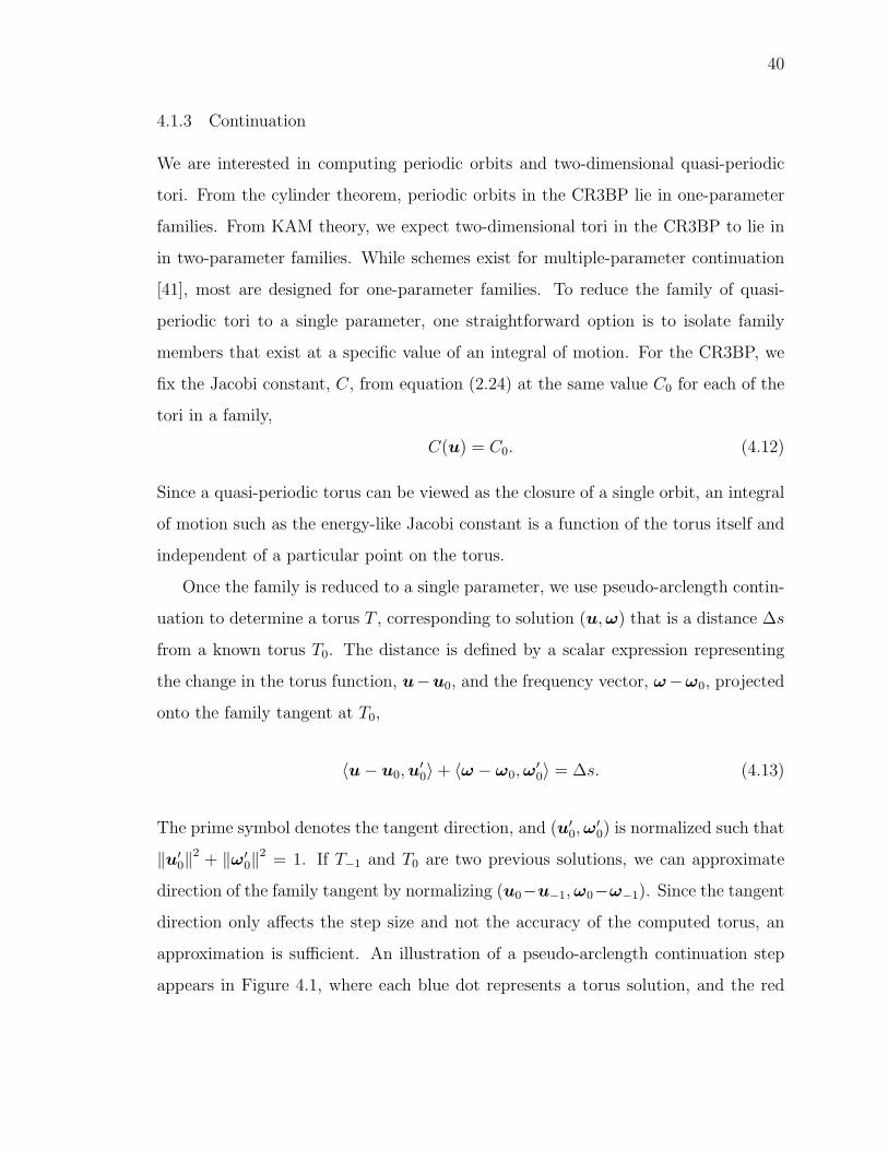
4.1.3 Continuation
We are interested in computing periodic orbits and two-dimensional quasi-periodic
tori. From the cylinder theorem, periodic orbits in the CR3BP lie in one-parameter
families. From KAM theory, we expect two-dimensional tori in the CR3BP to lie in
in two-parameter families. While schemes exist for multiple-parameter continuation
[41], most are designed for one-parameter families. To reduce the family of quasi-
periodic tori to a single parameter, one straightforward option is to isolate family
members that exist at a specific value of an integral of motion. For the CR3BP, we
fix the Jacobi constant, C, from equation (2.24) at the same value C0 for each of the
tori in a family,
C(u) = C0. (4.12)
Since a quasi-periodic torus can be viewed as the closure of a single orbit, an integral
of motion such as the energy-like Jacobi constant is a function of the torus itself and
independent of a particular point on the torus.
Once the family is reduced to a single parameter, we use pseudo-arclength contin-
uation to determine a torus T , corresponding to solution (u,ω) that is a distance ∆s
from a known torus T0. The distance is defined by a scalar expression representing
the change in the torus function, u−u0, and the frequency vector, ω−ω0, projected
onto the family tangent at T0,
〈u− u0,u′0〉+ 〈ω − ω0,ω
′0〉 = ∆s. (4.13)
The prime symbol denotes the tangent direction, and (u′0,ω′0) is normalized such that
‖u′0‖2 + ‖ω′0‖
2 = 1. If T−1 and T0 are two previous solutions, we can approximate
direction of the family tangent by normalizing (u0−u−1,ω0−ω−1). Since the tangent
direction only affects the step size and not the accuracy of the computed torus, an
approximation is sufficient. An illustration of a pseudo-arclength continuation step
appears in Figure 4.1, where each blue dot represents a torus solution, and the red
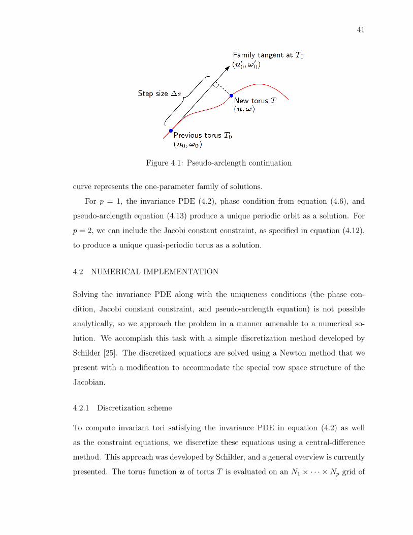
41
Figure 4.1: Pseudo-arclength continuation
curve represents the one-parameter family of solutions.
For p = 1, the invariance PDE (4.2), phase condition from equation (4.6), and
pseudo-arclength equation (4.13) produce a unique periodic orbit as a solution. For
p = 2, we can include the Jacobi constant constraint, as specified in equation (4.12),
to produce a unique quasi-periodic torus as a solution.
4.2 NUMERICAL IMPLEMENTATION
Solving the invariance PDE along with the uniqueness conditions (the phase con-
dition, Jacobi constant constraint, and pseudo-arclength equation) is not possible
analytically, so we approach the problem in a manner amenable to a numerical so-
lution. We accomplish this task with a simple discretization method developed by
Schilder [25]. The discretized equations are solved using a Newton method that we
present with a modification to accommodate the special row space structure of the
Jacobian.
4.2.1 Discretization scheme
To compute invariant tori satisfying the invariance PDE in equation (4.2) as well
as the constraint equations, we discretize these equations using a central-difference
method. This approach was developed by Schilder, and a general overview is currently
presented. The torus function u of torus T is evaluated on an N1 × · · · ×Np grid of

42
circularly-indexed points, Tp := {j = (j1, . . . , jp) | ji ∈ Z/NiZ}. The approximated
torus function u : Tp → Rn is defined such that u(j) := u(θ) where θi = jihi and
hi := 2π/Ni.
Operations equivalent to those on continuous torus functions are developed for
the discrete case. We approximate partial differentiation ∂/∂θi of torus state u(θ) on
the discrete domain by the operator ∂i,
∂iu(j) :=1
hi
l∑k=−l
cku(. . . , ji + k, . . .), (4.14)
where ck = −c−k are the central-difference coefficients. For the second-order approx-
imation (l = 1) of ∂u/∂θi: c0 = 0 and c1 = 1/2. For the fourth-order approximation
(l = 2): c0 = 0, c1 = 2/3, and c2 = −1/12. The inner product between two functions
v, w : Tp → Rn is defined such that
〈v, w〉 :=1
N1 · · ·Np
∑j∈Tp
〈v(j), w(j)〉 , (4.15)
which is a discrete version of equation (4.5).
4.2.2 Solution approach
Using the definitions of the discretized operators, we can write the discretized form
of the equations for tori of dimension p = 2 in the CR3BP, which we summarize in
the following system of equations:
0 = F 1j(u,ω) := f(u(j))−2∑i=1
ωi∂iu(j), for all j ∈ T2; (4.16a)
0 = F2i(u) := 〈∂iu0, u〉 , for all i ∈ {1, 2} ; (4.16b)
0 = F3(u) :=1
N1N2
∑j∈T2
C(u(j))− C0; (4.16c)
0 = F4(u,ω) := ku 〈u− u0, u′0〉+ kω 〈ω − ω0,ω
′0〉 −∆s. (4.16d)

43
A nearby family member T0, that is assumed to be already computed, has discrete
torus function u0 and frequency vector ω0. The Jacobi constant C is averaged over
the entire torus in equation (4.16c) to distribute numerical sensitivities. Also, we add
coefficients ku and kω to the pseudo-arclength equation (4.16d) to allow more control
over the stepping process. Typical choices are ku = 1 and kω = 0 to prevent falling
back to a periodic orbit where it is possible u− u0 = 0 but ω − ω0 6= 0.
We solve the system of equations (4.16) for u and ω using a Newton method. If
u is represented as a column vector of length nN1N2, the system of equations to be
solved is ∂F 1/∂u ∂F 1/∂ω
∂F 2/∂u 0
∂F3/∂u 0
∂F4/∂u ∂F4/∂ω
δu
δω
= −
F 1(u,ω)
F 2(u)
F3(u)
F4(u,ω)
, (4.17)
where u 7→ u + δu and ω 7→ ω + δω are updated at each iteration. Details of the
sparse structure of submatrix ∂F 1/∂u in the Jacobian is available in Schilder [25].
Note that the structure of the CR3BP leads to an (nN1N2+4)×(nN1N2+2) Jaco-
bian matrix. Though this linear system appears to be overdetermined, KAM theory
suggests that, for a Hamiltonian system such as the CR3BP, a solution does, in fact,
exist. Therefore, two columns can be added to make the Jacobian square, provided
they are not already in the column space. Consider these columns as corresponding
to two “artificial” external parameters λ1 = λ2 = 0 that do not affect the dynamics at
value zero. A suitable choice is the random generation of vectors v1,v2 ∈ RnN1N2+4
resulting in the linear system∂F 1/∂u ∂F 1/∂ω
∂F 2/∂u 0
∂F3/∂u 0
∂F4/∂u ∂F4/∂ω
v1 v2
δu
δω
δλ1
δλ2
= −
F 1(u,ω)
F 2(u)
F3(u)
F4(u,ω)
. (4.18)
Since v1 and v2 are random, the Jacobian should be square and nonsingular. We
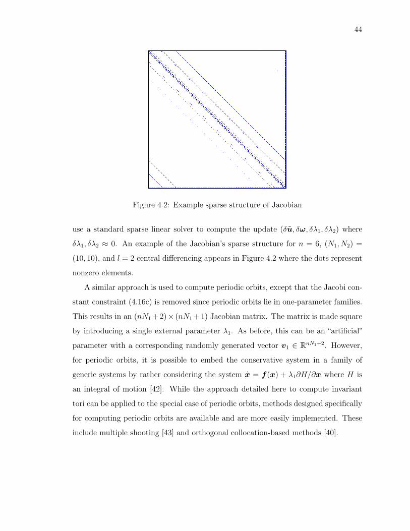
44
Figure 4.2: Example sparse structure of Jacobian
use a standard sparse linear solver to compute the update (δu, δω, δλ1, δλ2) where
δλ1, δλ2 ≈ 0. An example of the Jacobian’s sparse structure for n = 6, (N1, N2) =
(10, 10), and l = 2 central differencing appears in Figure 4.2 where the dots represent
nonzero elements.
A similar approach is used to compute periodic orbits, except that the Jacobi con-
stant constraint (4.16c) is removed since periodic orbits lie in one-parameter families.
This results in an (nN1 + 2)× (nN1 + 1) Jacobian matrix. The matrix is made square
by introducing a single external parameter λ1. As before, this can be an “artificial”
parameter with a corresponding randomly generated vector v1 ∈ RnN1+2. However,
for periodic orbits, it is possible to embed the conservative system in a family of
generic systems by rather considering the system x = f(x) + λ1∂H/∂x where H is
an integral of motion [42]. While the approach detailed here to compute invariant
tori can be applied to the special case of periodic orbits, methods designed specifically
for computing periodic orbits are available and are more easily implemented. These
include multiple shooting [43] and orthogonal collocation-based methods [40].

45
4.2.3 Regularization
The discretization scheme presented uses a evenly-spaced mesh of torus angles θ =
(θ1, . . . , θp), which are related linearly to time, i.e., θ = ωt. However, a nonlinear
system can possess a vector field that is far from uniform in certain regions. This
behavior is particularly evident in the CR3BP near each of the two primary bodies at
which the equations of motion (2.14) and (2.22) have a singularity. If we consider a
trajectory that passes in the vicinity of a primary, states vary much more rapidly with
respect to time t nearer the primary. With uniform time steps, numerical computation
in sensitive regions can be highly inaccurate. We can, however, reparameterize a
trajectory using a new time s, which we define to “slow down” as the trajectory nears
the singularity. The two times are related by the scalar differential equation
ds
dt= g(x), (4.19)
which is known as a (generalized) Sundman transformation. Given a trajectory x :
[0, t] 7→ Rn propagated for t time units, the equivalent time s is given by
s(t) =
ˆ t
0
g(x(t′)) dt′. (4.20)
Alternatively, if the trajectory x : [0, s] 7→ Rn is parameterized by the new time s,
the standard time t can be determined from
t(s) =
ˆ s
0
1
g(x(s′))ds′. (4.21)
The choice of function g(x) to optimally scale time is system dependent. For the
two-body problem, Roy [27] suggests the choice g(x) = d−k, where d is the distance
between the bodies and k = 1 or 2. Leimkuhler [44] presents the choice k = 3/2
to preserve a scaling symmetry and also notes that numerical tests show it to be
approximately optimal. We modify this choice for the CR3BP and relate the times
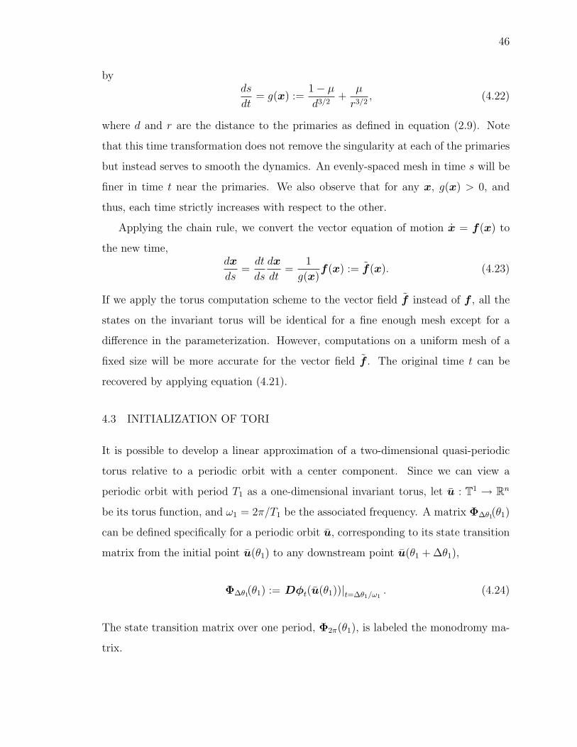
46
byds
dt= g(x) :=
1− µd3/2
+µ
r3/2, (4.22)
where d and r are the distance to the primaries as defined in equation (2.9). Note
that this time transformation does not remove the singularity at each of the primaries
but instead serves to smooth the dynamics. An evenly-spaced mesh in time s will be
finer in time t near the primaries. We also observe that for any x, g(x) > 0, and
thus, each time strictly increases with respect to the other.
Applying the chain rule, we convert the vector equation of motion x = f(x) to
the new time,dx
ds=dt
ds
dx
dt=
1
g(x)f(x) := f(x). (4.23)
If we apply the torus computation scheme to the vector field f instead of f , all the
states on the invariant torus will be identical for a fine enough mesh except for a
difference in the parameterization. However, computations on a uniform mesh of a
fixed size will be more accurate for the vector field f . The original time t can be
recovered by applying equation (4.21).
4.3 INITIALIZATION OF TORI
It is possible to develop a linear approximation of a two-dimensional quasi-periodic
torus relative to a periodic orbit with a center component. Since we can view a
periodic orbit with period T1 as a one-dimensional invariant torus, let u : T1 → Rn
be its torus function, and ω1 = 2π/T1 be the associated frequency. A matrix Φ∆θ1(θ1)
can be defined specifically for a periodic orbit u, corresponding to its state transition
matrix from the initial point u(θ1) to any downstream point u(θ1 + ∆θ1),
Φ∆θ1(θ1) := Dφt(u(θ1))|t=∆θ1/ω1. (4.24)
The state transition matrix over one period, Φ2π(θ1), is labeled the monodromy ma-
trix.

47
Let us consider a periodic orbit with a center component. This corresponds to
a monodromy matrix Φ2π(0) that possesses an eigenvalue on the unit circle eiα =
cosα + i sinα and an associated complex eigenvector y(0) ∈ Cn, ‖y(0)‖ = 1. It can
be demonstrated that the monodromy matrix Φ2π(θ1) also has the same eigenvalue
eiα and an eigenvector Φθ1(0)y(0). Since any eigenvector times a complex scalar is
also an eigenvector, we select the desired form of the eigenvector of Φ2π(θ1) to be
y(θ1) := e−iαθ1/2πΦθ1(0)y(0). (4.25)
The state transition matrix Φθ1(0) not only shifts the eigenvector y(0) to correspond
to point u(θ1), but it also follows the rotation about the periodic orbit from the
flow. The term e−iαθ1/2π corresponds to a rotation in the complex plane by the angle
−αθ1/2π, and is included to cancel the rotation from the flow. As a consequence,
equation (4.25) is defined such that y : T1 → Cn is periodic; for example, y(2π) =
e−iαΦ2π(0)y(0) = e−iαeiαy(0) = y(0).
We now define a torus function perturbation u : T2 → Rn,
u(θ1, θ2) := Re[eiθ2y(θ1)
]= cos θ2 Re [y(θ1)]− sin θ2 Im [y(θ1)] .
(4.26)
Note that for each θ1, u(θ1, ·) is an ellipse in Rn with axes Re [y(θ1)] and Im [y(θ1)].
For example, the evolution of the axes for a halo orbit in the CR3BP appears in Figure
4.3. From the definition in equation (4.26), we can demonstrate that the monodromy
matrix Φ2π(θ1) maps a point u(θ1, θ2) on this ellipse to a point u(θ1, θ2 + α) shifted
by angle α on the same ellipse:
Φ2π(θ1)u(θ1, θ2) = Φ2π(θ1)Re[eiθ2y(θ1)
]= Re
[eiθ2Φ2π(θ1)y(θ1)
]= Re
[eiθ2eiαy(θ1)
]= u(θ1, θ2 + α).
(4.27)

48
Figure 4.3: Eigenvector components around halo orbit
Therefore, a linear approximation of the torus is available from
u(θ1, θ2) = u(θ1) + εu(θ1, θ2), (4.28)
where ε ∈ R fixes the size of the torus. Its frequencies are ω = (ω1, ω2) = (2π/T1, α/T1).
Note that any angle α = α0 + 2πk, k ∈ Z, such that cosα + i sinα is an eigenvalue
of the monodromy matrix, can be selected since a unimodular transformation of the
frequency vector ω also corresponds to a suitable parameterization of the torus. This
approach can be generalized without much difficulty to yield initial approximations
for tori of dimension p > 2 from periodic orbits having a monodromy matrix with
more than one pair of complex conjugate eigenvalues.
4.4 COMPUTATIONAL SCHEME
A flow chart providing an overview of the scheme for computing tori appears in Figure
4.4. The two-dimensional torus is first initialized from a periodic orbit with a center
component. We then use a Newton method to iterate until the discretized torus
equations are satisfied. Once they are satisfied, the next torus in the family can be

49
Figure 4.4: Computational approach
predicted, and the process repeats until a certain number of tori are computed or the
discretized equations can no longer be solved.
Since the torus function u possesses a natural parameterization via angles θ ∈ Tp,
it is well-suited to generating individual orbits. After a torus is computed, we can
determine a single quasi-periodic orbit on its surface by interpolating the discretized
torus function u on the evenly-spaced mesh points Tp. In the current study, a p = 2-
parameter cubic spline u∗ : T2 → Rn is generated over the domain [0, 2π] × [0, 2π]
with periodic end conditions. This is possible using a variety of software packages.
Then, from any starting point θ0 ∈ T2, we approximate the state at time t as
x(t) = u∗((θ0 + ωt) (mod 2π)). (4.29)
A trajectory generated in this manner is suitable as input to a higher-order corrections
scheme or to initiate the transition to an ephemeris model using a process such as
multiple shooting. Since the cubic spline can be evaluated efficiently once it is com-
puted, quasi-periodic orbits from various starting points θ0 can be generated with
minimal computational effort.
Examples of this scheme applied to a Lissajous trajectory and a quasi-halo orbit

50
(mesh points) (torus surface) (trajectory)
Figure 4.5: Steps for Lissajous orbit computation
(mesh points) (torus surface) (trajectory)
Figure 4.6: Steps for quasi-halo orbit computation
in the CR3BP appear in Figures 4.5 and 4.6, which illustrate the mesh points from
the discretization of the PDE, the corresponding invariant torus surface generated
from a two-parameter cubic spline, and the quasi-periodic orbit that lies on the torus
surface. These quasi-periodic tori are investigated further in the next chapter.

51
CHAPTER 5
FAMILIES OF TORI IN THE EARTH-MOON CR3BP
In this chapter we demonstrate the approach developed to compute invariant tori in
the CR3BP. Specifically we consider tori of dimension zero, one, and two in the Earth-
Moon system (µ = 0.012151). We first investigate the stability of the libration points
and qualitatively describe the dynamics in their vicinity. The center component of
the linearized dynamics about the libration points corresponds to emanating families
of periodic orbits. Sample families are computed, and orbits with quasi-periodic
motion in their vicinity are identified. We select some representative periodic orbits
from which to initialize families of two-dimensional quasi-periodic tori that exist at a
fixed value of Jacobi constant. While not intended to be a complete study of quasi-
periodic motion in the CR3BP, the sample families illustrate the capability of the
computational scheme.
5.1 LIBRATION POINTS
The zero-dimensional tori in the CR3BP consist of the five libration points, which
can be determined using the approach discussed previously in Section 2.3. We are
interested in studying the phase space structure near these points, particularly the
higher-dimensional invariant tori. The dynamics in the vicinity of the libration points
can be qualitatively understood using the methods from Section 3.1 and the stable,
unstable, and center manifold theorems for continuous flows. To apply these theo-
rems, we consider the eigenvalues of the 6 × 6 matrix Df(x) corresponding to the
linearization of the CR3BP vector field f relative to the libration point x. Since
the eigenvalues of the matrix Df(x) are symmetric across the imaginary axis for
a Hamiltonian system [36], we categorize the stability type for each libration point

52
Table 5.1: Linear stability of libration points
0 ≤ µ < µcrit µcrit < µ ≤ 0.5L1 center× center× saddleL2 center× center× saddleL3 center× center× saddleL4 center× center× center center× center× saddleL5 center× center× center center× center× saddle
in a system with mass parameter µ using the three components listed in Table 5.1.
The label “center” implies a pair of eigenvalues with zero real part. The label “sad-
dle” denotes a pair of eigenvalues with nonzero real part, one eigenvalue possessing a
negative real part and the other a positive real part.
For any CR3BP system, a linearization relative to the collinear libration points
L1, L2, and L3 yields two pairs of eigenvalues corresponding to center motion and
one pair of eigenvalues that represent a saddle. Applying the stable, unstable, and
center manifold theorem, we conclude that there exists a four-dimensional center
manifold, a one-dimensional stable manifold, and a one-dimensional unstable manifold
for each of these libration points. Since there is at least one unstable direction, the
collinear libration points are termed to be unstable. Locally, we expect an arbitrary
perturbation to the libration point state to grow exponentially in time.
Unlike the collinear libration points, the stability of the triangular libration points,
L4 and L5, is system dependent. As demonstrated in Szebehely [26], for systems with
a mass parameter less than a critical value, µ < µcrit = 0.038521, all the pairs of
eigenvalues correspond to center motion and, thus, there is a six-dimensional center
manifold. This includes the Earth-Moon CR3BP system. On the other hand, a mass
parameter µ > µcrit results in one pair of eigenvalues associated with saddle behavior.
In this case, L4 and L5 are unstable, and the situation is similar to that of the collinear
libration points. An analysis for the system µ = µcrit is more complicated; further
discussion of the Hamiltonian Hopf bifurcation that occurs in this case is available in
Meyer [36].
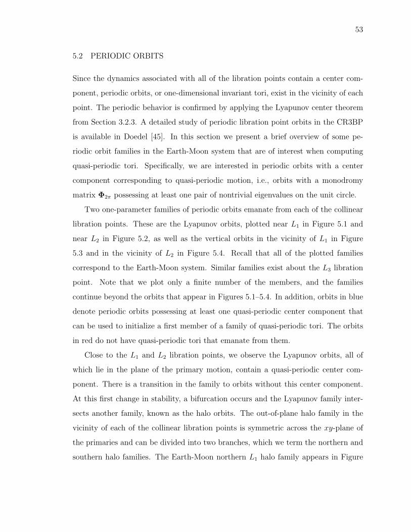
53
5.2 PERIODIC ORBITS
Since the dynamics associated with all of the libration points contain a center com-
ponent, periodic orbits, or one-dimensional invariant tori, exist in the vicinity of each
point. The periodic behavior is confirmed by applying the Lyapunov center theorem
from Section 3.2.3. A detailed study of periodic libration point orbits in the CR3BP
is available in Doedel [45]. In this section we present a brief overview of some pe-
riodic orbit families in the Earth-Moon system that are of interest when computing
quasi-periodic tori. Specifically, we are interested in periodic orbits with a center
component corresponding to quasi-periodic motion, i.e., orbits with a monodromy
matrix Φ2π possessing at least one pair of nontrivial eigenvalues on the unit circle.
Two one-parameter families of periodic orbits emanate from each of the collinear
libration points. These are the Lyapunov orbits, plotted near L1 in Figure 5.1 and
near L2 in Figure 5.2, as well as the vertical orbits in the vicinity of L1 in Figure
5.3 and in the vicinity of L2 in Figure 5.4. Recall that all of the plotted families
correspond to the Earth-Moon system. Similar families exist about the L3 libration
point. Note that we plot only a finite number of the members, and the families
continue beyond the orbits that appear in Figures 5.1–5.4. In addition, orbits in blue
denote periodic orbits possessing at least one quasi-periodic center component that
can be used to initialize a first member of a family of quasi-periodic tori. The orbits
in red do not have quasi-periodic tori that emanate from them.
Close to the L1 and L2 libration points, we observe the Lyapunov orbits, all of
which lie in the plane of the primary motion, contain a quasi-periodic center com-
ponent. There is a transition in the family to orbits without this center component.
At this first change in stability, a bifurcation occurs and the Lyapunov family inter-
sects another family, known as the halo orbits. The out-of-plane halo family in the
vicinity of each of the collinear libration points is symmetric across the xy-plane of
the primaries and can be divided into two branches, which we term the northern and
southern halo families. The Earth-Moon northern L1 halo family appears in Figure

54
Figure 5.1: L1 Lyapunov family Figure 5.2: L2 Lyapunov family
Figure 5.3: L1 vertical family Figure 5.4: L2 vertical family

55
Figure 5.5: L1 northern halo family Figure 5.6: L2 northern halo family
5.5, and the northern L2 family is plotted in Figure 5.6. Note that these families
extend beyond the orbits that are illustrated. The green orbit in each figure denotes
the bifurcating orbit and belongs to both the Lyapunov and halo families. Consistent
with the previous plots, we use the color blue to identify periodic orbits from which
quasi-periodic tori emanate. Another family of periodic orbits, identified as the axial
family, bifurcates from the Lyapunov family at its second change in stability, and
ends at a bifurcation with the vertical family at its first change in stability. However,
none of the axial orbits contain a quasi-periodic center component.
Three families of periodic orbits emanate from each of the stable L4 and L5 tri-
angular libration points in the Earth-Moon system. These families are symmetric
across the xz-plane. Two of the families, termed the short- and long-period families,
lie in the primaries’ plane. The third family consists of vertical orbits similar to those
associated with the collinear libration points. This vertical orbit family undergoes a
bifurcation to a family of orbits labeled the W -family by Doedel [45] and a portion
of the family’s northern branch appears in Figure 5.7. If the W -family is continued

56
Figure 5.7: L4 northern W -orbit family
further, it intersects the L1 halo family. The green orbit represents the intersection
with the vertical family. Since the W -orbits do not contain any symmetries but have
quasi-periodic motion in their vicinity, we use it to verify that the computational
scheme works for tori with which we have little intuition.
5.3 QUASI-PERIODIC TORI
Families of two-dimensional quasi-periodic invariant tori emanating from periodic
orbits in the CR3BP can be computed using the scheme presented in Chapter 4.
Since the phase space near the collinear libration points includes a four-dimensional
center manifold, we predict the dynamics on the manifold to primarily consist of
motion on two-dimensional tori. We base this prediction on the observation that the
tori lie in two-parameter families and, thus, primarily fill the four-dimensional space.
The prevalence of two-dimensional tori motivates their study and computation as a
means to better understand the center manifold of the collinear libration points. In
addition, two-dimensional quasi-periodic tori emanate from periodic orbits near the

57
triangular libration points.
The computation scheme is implemented in MATLAB R© R2009b on a laptop with
a 2.66 GHz Intel R© CoreTM 2 Duo processor. Each Newton update of equation (4.18) is
solved using the sparse LU factorization built into MATLAB, and the Spline Toolbox
is used to generate the quasi-periodic trajectory from equation (4.29). While care is
taken to use vectorized operations, additional performance optimizations are possible.
A family of tori, generally identified as the Lissajous tori, emanates from the
Lyapunov orbits in the vicinity of the collinear libration points. We select an L1
Lyapunov orbit in the Earth-Moon system with Jacobi constant C = 3.179, which
corresponds to a maximum y-amplitude of 0.450, from which to initialize a small quasi-
periodic torus. This choice of Jacobi constant is not unique, and any L1 Lyapunov
orbit with a quasi-periodic center component, as identified in Figure 5.1, can be
selected. The torus is computed on an N1 × N2 = 40 × 40 grid with fourth-order
central differencing. We then use pseudo-arclength continuation to generate a family
of tori with a fixed Jacobi constant C. Six members of this family appear in Figure
5.8. We observe that these Lissajous tori terminate at an L1 vertical orbit, also with
C = 3.179. A total of 13 members of the family are computed in 90 seconds with
roughly 95 percent of the time spent solving the linear system from equation (4.18).
The Jacobian is of dimension 9, 604 × 9, 604 with approximately 0.17 percent of the
elements nonzero. This sparsity underlines the importance of using a sparse linear
system solver. Similar quasi-periodic families are observed to connect some of the
planar Lyapunov periodic orbits in the vicinity of L2 and L3 and the short-period
orbits near L4 and L5 to the corresponding vertical periodic orbits.
Many of the halo orbits, which branch from the collinear libration points’ Lya-
punov orbits, have nearby quasi-periodic motion. These orbits are marked in Figures
5.5–5.6 for L1 and L2. An sample family of L2 quasi-halo tori with Jacobi constant
C = 3.132 is plotted in Figure 5.9. Each torus is computed on an N1 ×N2 = 75× 25
grid, which corresponds to an 11, 254 × 11, 254 Jacobian that is about 0.15 percent
dense. It requires 58 seconds total to compute 10 family members. The continuation
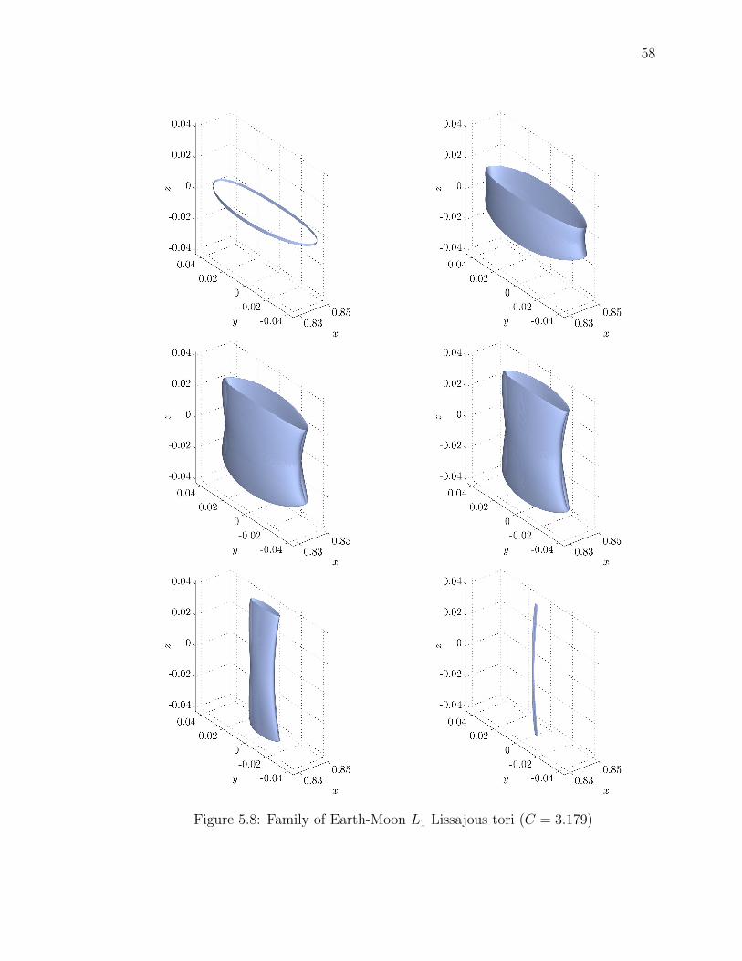
58
Figure 5.8: Family of Earth-Moon L1 Lissajous tori (C = 3.179)
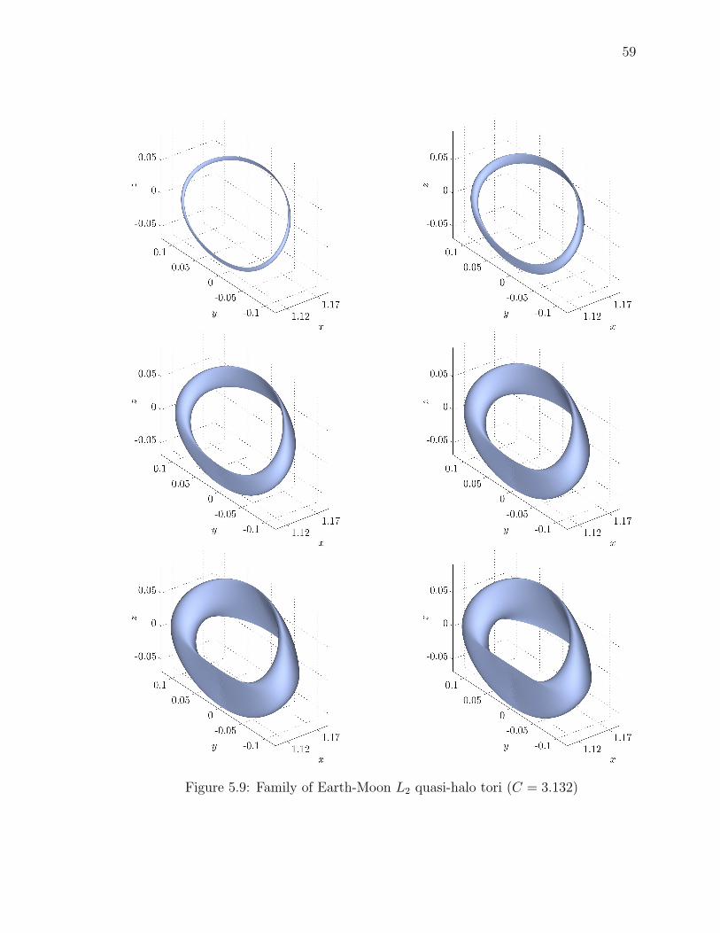
59
Figure 5.9: Family of Earth-Moon L2 quasi-halo tori (C = 3.132)

60
ends when the “edges” of the tori approach the xy-plane; for an example, see the last
torus appearing in Figure 5.9.
When the tori are computed on a uniform mesh, there are numerical difficulties
generating a family from a halo orbit that passes near to a primary body, where the
dynamics change much faster. However, we apply the regularization scheme from
Section 4.2.3 to mitigate these issues. An L2 halo with Jacobi constant C = 3.038 is
selected to initialize the quasi-halo family, which appears in Figure 5.10. By “slowing”
the time near the primary, the N1 ×N2 = 100× 25 mesh becomes significantly finer
in this region allowing convergence. Using a mesh of the same dimensions without
regularization, the updates become very large and the Newton method is unable to
converge on a solution. If the entire mesh is made finer (where N1 is approximately
2,000), convergence without regularization appears theoretically possible, but solving
the associated linear system for the Newton update is not feasible on the current
computer hardware.
The computational scheme is designed to require only an appropriate initial guess
for a first torus, and it does not require any modification between families. To demon-
strate this capability, we select a northern L4 W -orbit from Figure 5.7 with Jacobi
constant C = 2.012. Since the orbit has a center component corresponding to quasi-
periodic motion, the torus initialization scheme is applied. Even though the W -orbits
do not possess any symmetries and there is no prior insight into the appearance of a
quasi-periodic torus about this orbit, the scheme is still successful. The family of tori
near the periodic orbit appears in Figure 5.11. Part of a quasi-periodic trajectory on
the surface of one of the tori is plotted in Figure 5.12.

61
Figure 5.10: Family of Earth-Moon L2 quasi-halo tori (C = 3.038)
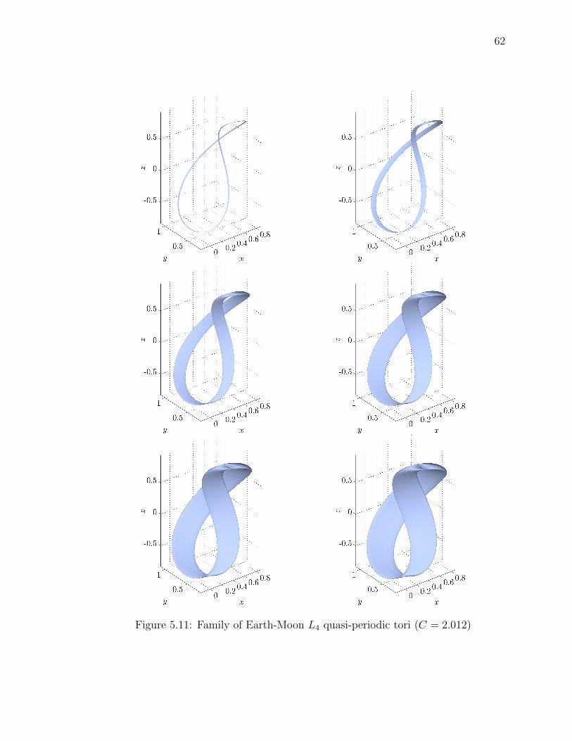
62
Figure 5.11: Family of Earth-Moon L4 quasi-periodic tori (C = 2.012)
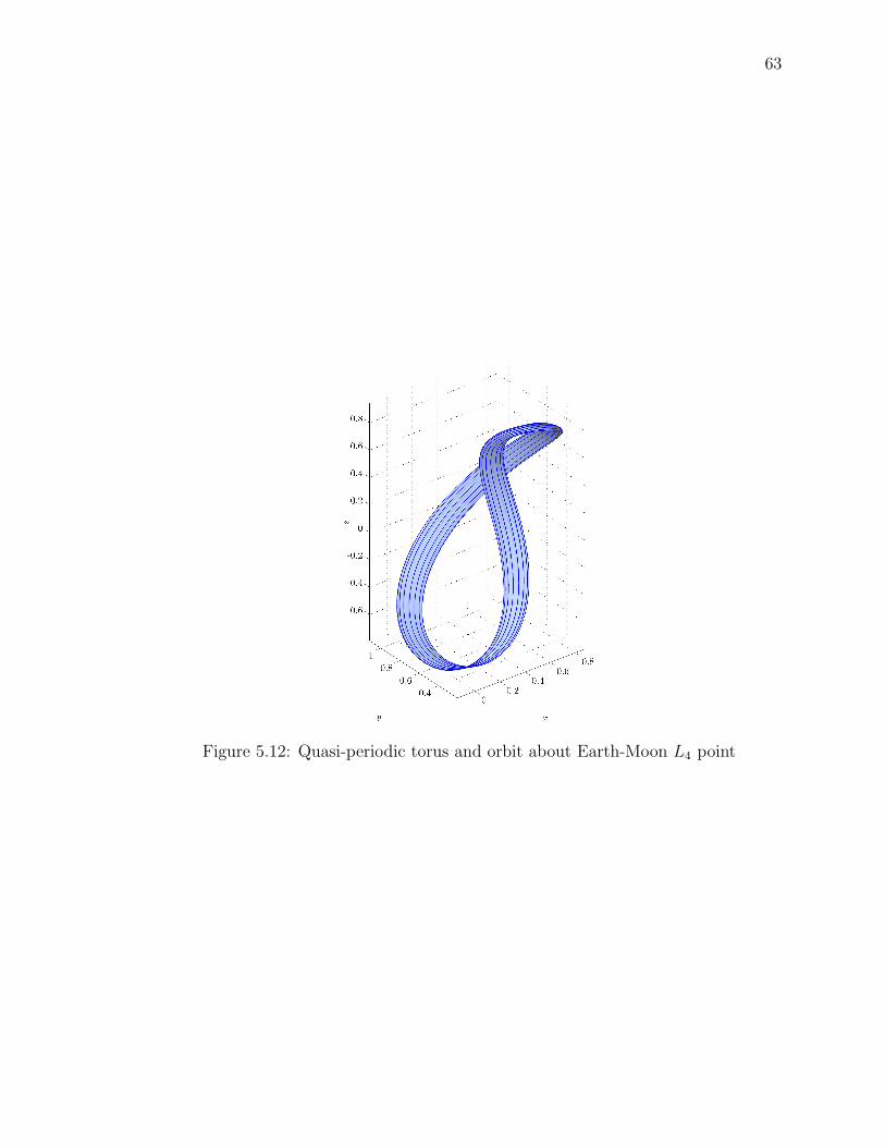
63
Figure 5.12: Quasi-periodic torus and orbit about Earth-Moon L4 point

64
CHAPTER 6
SUMMARY AND RECOMMENDATIONS
In this chapter, we summarize the solution approach developed and the results con-
firming the approach’s validity in the CR3BP. In addition, we provide recommenda-
tions for future work.
6.1 SUMMARY
The primary goal of this work is a framework for computing quasi-periodic invari-
ant tori in the CR3BP. We based the approach on a scheme developed by Schilder
[25] for generic dynamical systems that is applicable to tori of any dimension. We
include suitable modifications to incorporate the CR3BP’s special structure, notably
that families of tori exist without any external parameters. This extends the appli-
cability of the method to systems with an integral of motion, notably Hamiltonian
systems. We are able to uniquely describe a given invariant torus by a torus function
satisfying an invariance partial differential equation and a set of phase conditions.
However, since tori lie in families, additional constraints are necessary to identify a
particular torus. First, we incorporate a Jacobi constant constraint to reduce two-
parameter families of two-dimensional quasi-periodic tori in the CR3BP to a single
parameter. This constraint is not necessary for periodic orbits, which naturally lie
in one-parameter families. Then, pseudo-arclength continuation is exploited to step
along the one-parameter families.
Central-difference discretization of the continuous equations enables us to itera-
tively compute the torus function, along with its associated frequencies, on a uniform
grid. We introduce a simple bordering scheme associated with artificial external pa-
rameters that allows the Newton update to be efficiently computed. In addition, we
65
offer a regularization scheme to compute tori in sensitive regimes of the CR3BP. To
begin the correction and continuation process, we present a linear approximation of a
two-dimensional invariant torus emanating from a periodic orbit with a quasi-periodic
center component. Once a torus is computed, we can readily generate a quasi-periodic
trajectory from an arbitrary starting point on its surface using spline interpolation.
We demonstrate the computational scheme’s effectiveness by computing invariant
tori in the Earth-Moon CR3BP. Since the center manifold associated with each of the
collinear libration points is four-dimensional, the study of two-dimensional tori lying
in two-parameter families is of interest. Families of periodic orbits about the libration
points are provided, and sample orbits with quasi-periodic motion in their vicinity
are selected to initialize families of two-dimensional quasi-periodic tori. We present
some members from the continuation process where all the tori possess a fixed Jacobi
constant value. The regularization scheme enables the inclusion of families that pass
near one of the primary bodies. The results demonstrate that the procedure for
generating families in the CR3BP is tractable with standard computing resources.
6.2 RECOMMENDATIONS
The current work leads to additional areas for exploration. An adaptive mesh refine-
ment scheme, beyond the regularization approach currently used, may enable more
accurate computation of tori near the primaries. A comparison with the efficiency of
other torus computation approaches is also warranted, though this is challenging due
to the complexity of the available schemes for computing quasi-periodic invariant tori.
In addition, exploiting high-performance computing tools would allow faster results
and, as a consequence, more complicated problems will become feasible. In particular,
a faster solution of the sparse linear system solved at each Newton update, where a
majority of the computational time is spent, could significantly speed up the process.
Quasi-periodic trajectories have numerous mission applications, and their role in
the mission design process should be investigated. An important consideration is the
stability of the tori. We expect a torus close to a periodic orbit with an unstable
66
component to be unstable as well, but the stability could change as we continue along
a family. Exploring the stable and unstable manifolds of quasi-periodic invariant
tori would also help clarify transfer options. The approach here can also be used
to compute additional families in the Earth-Moon system as well as other systems.
Furthermore, the scheme can be extended with little modification to compute higher-
dimensional tori, particularly three-dimensional tori in the vicinity of the triangular
libration points. A thorough investigation of the torus families should provide a
clearer picture of the libration points’ center manifolds.

LIST OF REFERENCES

67
LIST OF REFERENCES
[1] Gerard Gomez, Angel Jorba, Josep J. Masdemont, and Carles Simo. Study ofthe transfer from the Earth to a halo orbit around the equilibrium point L1.Celestial Mechanics and Dynamical Astronomy, 56(4):541–562, 1993.
[2] Kathleen C. Howell, Brian T. Barden, and Martin W. Lo. Application of dynam-ical systems theory to trajectory design for a libration point mission. Journal ofthe Astronautical Sciences, 45(2):161–178, 1997.
[3] Brian T. Barden and Kathleen C. Howell. Fundamental motions near collinearlibration points and their transitions. Journal of the Astronautical Sciences, 46(4):361–378, 1998.
[4] Edmund T. Whittaker. A Treatise on the Analytical Dynamics of Particles andRigid Bodies. Cambridge University Press, 1904.
[5] Karl F. Sundman. Memoire sur le probleme des trois corps. Acta Mathematica,36:105–179, 1912.
[6] Leonhard Euler. De motu rectilineo trium corporum se mutuo attrahentium.Opera Omnia, 25:1–411, 1767.
[7] Carl G. J. Jacobi. Sur le mouvement d’un point et sur un cas particulier duprobleme des trois corps. Comptes Rendus, 3:59–61, 1836.
[8] George W. Hill. Researches into the lunar theory. American Journal of Mathe-matics, 1:5–26, 129–147, 245–260, 1878.
[9] J. Henri Poincare. Sur le probleme des trois corps et les equations de la dy-namique. Acta Mathematica, 13:1–270, 1890.
[10] J. Henri Poincare. Les Methodes Nouvelles de la Mecanique Celeste, volume 1-3.Gauthier-Villars, 1892-1899. Republished by Blanchard, Paris, 1987.
[11] George D. Birkhoff. Quelques theoremes sur le mouvement des systemes dy-namiques. Bulletin de la Societe Mathematique de France, 40:305–323, 1912.
[12] June E. Barrow-Green. Poincare and the Three Body Problem. American Math-ematical Society/London Mathematical Society, 1997.
[13] George H. Darwin. Periodic orbits. Acta Mathematica, 21:99–242, 1897.

68
[14] Henry C. Plummer. On oscillating satellites, 1. Monthly Notices of the RoyalAstronomical Society, 63(8):436–443, 1903.
[15] Henry C. Plummer. On oscillating satellites, 2. Monthly Notices of the RoyalAstronomical Society, 64(2):98–105, 1903.
[16] Forest R. Moulton. Periodic Orbits. Carnegie Institution of Washington, 1920.
[17] Robert W. Farquhar. The Control and Use of Libration-Point Satellites. Ph.D.dissertation, Stanford University, Stanford, California, July 1968.
[18] Robert W. Farquhar and Ahmed A. Kamel. Quasi-periodic orbits about thetranslunar libration point. Celestial Mechanics and Dynamical Astronomy, 7(4):458–473, 1973.
[19] David L. Richardson and Noel D. Cary. A uniformly valid solution for motionabout the interior libration point of the perturbed elliptic-restricted problem.In Proceedings of the AAS/AIAA Astrodynamics Specialist Conference. Nassau,Bahamas, July 1975.
[20] Angel Jorba and Josep J. Masdemont. Dynamics in the center manifold of therestricted three-body problem. Physica D, 132(1-2):189–213, 1999.
[21] Gerard Gomez, Josep J. Masdemont, and Carles Simo. Quasihalo orbits associ-ated with libration points. Journal of the Astronautical Sciences, 46(2):135–176,1998.
[22] Angel Jorba. Numerical computation of the normal behavior of invariant curvesof n-dimensional maps. Nonlinearity, 14(5):943–976, 2001.
[23] Angel Jorba and Estrella Olmedo. On the computation of reducible invarianttori in a parallel computer. Preprint, 2008.
[24] Gerard Gomez and Josep M. Mondelo. The dynamics around the collinear equi-librium points of the RTBP. Physica D, 157(4):283–321, 2001.
[25] Frank Schilder, Hinke M. Osinga, and Werner Vogt. Continuation of quasi-periodic invariant tori. SIAM Journal on Applied Dynamical Systems, 4(3):459–488, 2005.
[26] Victor G. Szebehely. Theory of Orbits: The Restricted Problem of Three Bodies.Academic Press, 1967.
[27] Archie E. Roy. Orbital Motion. Institute of Physics, 4th edition, 2005.
[28] John E. Prussing and Bruce A. Conway. Orbital Mechanics. Oxford UniversityPress, 1993.

69
[29] NASA Jet Propulsion Laboratory. HORIZONS system, June 2010. URL http:
//ssd.jpl.nasa.gov/?horizons.
[30] Donald T. Greenwood. Classical Dynamics. Prentice-Hall, 1977.
[31] Stephen Wiggins. Introduction to Applied Nonlinear Dynamical Systems andChaos. Springer-Verlag, 2nd edition, 2003.
[32] John M. Guckenheimer and Philip J. Holmes. Nonlinear Oscillations, DynamicalSystems, and Bifurcations of Vector Fields. Springer-Verlag, 1983.
[33] Lawrence M. Perko. Differential Equations and Dynamical Systems. Springer-Verlag, 1991.
[34] Gilbert Strang. Linear Algebra and Its Applications. Cengage Learning, 4thedition, 2005.
[35] Morris W. Hirsch and Stephen Smale. Differential Equations, Dynamical Sys-tems, and Linear Algebra. Academic Press, 1974.
[36] Kenneth R. Meyer and Glen R. Hall. Introduction to Hamiltonian DynamicalSystems and the N-Body Problem. Springer-Verlag, 1992.
[37] Yuri A. Kuznetsov. Elements of Applied Bifurcation Theory. Springer-Verlag,3rd edition, 2004.
[38] Stephen Wiggins. Normallly Hyperbolic Invariant Manifolds in Dynamical Sys-tems. Springer-Verlag, 1994.
[39] Hendrik W. Broer, George B. Huitema, and Mikhail B. Sevryuk. Quasi-PeriodicMotions in Families of Dynamical Systems. Lecture Notes in Mathematics.Springer-Verlag, 1996.
[40] Eusebius J. Doedel, Herbert B. Keller, and Jean Pierre Kernevez. Numericalanalysis and control of bifurcation problems: (II) Bifurcations in infinite dimen-sions. International Journal of Bifurcation and Chaos, 1(4):745–772, 1991.
[41] Michael E. Henderson. Multiple parameter continuation: Computing implicitlydefined k-manifolds. International Journal of Bifurcation and Chaos, 12(3):451–476, 2002.
[42] Francisco J. Munoz-Almaraz, Emilio Freire, Jorge Galan-Vioque, Eusebius J.Doedel, and Andre Vanderbauwhede. Continuation of periodic orbits in conser-vative and Hamiltonian systems. Physica D, 181(1–2):1–38, 2003.
[43] Herbert B. Keller. Numerical Solution of Two Point Boundary Value Problems.Society for Industrial and Applied Mathematics, 1976.
70
[44] Benedict Leimkuhler and Sebastian Reich. Simulating Hamiltonian Dynamics.Cambridge University Press, 2004.
[45] Eusebius J. Doedel, Volodymyr A. Romanov, Randy C. Paffenroth, Herbert B.Keller, Donald J. Dichmann, Jorge Galan-Vioque, and Andre Vanderbauwhede.Elemental periodic orbits associated with the libration points in the circularrestricted 3-body problem. International Journal of Bifurcation and Chaos, 17(8):2625–2677, 2007.